Embed Size (px)
Citation preview
Volume Change Consideration in Determining Appropriate
Unsaturated Soil Properties for Geotechnical Applications
by
Elham Bani Hashem
A Dissertation Presented in Partial Fulfillment
of the Requirements for the Degree
Doctor of Philosophy
Approved April 2013 by the
Graduate Supervisory Committee:
Sandra Houston, Chair
Edward Kavazanjian
Claudia Zapata
ARIZONA STATE UNIVERSITY
May 2013
i
ABSTRACT
Unsaturated soil mechanics is becoming a part of geotechnical engineering
practice, particularly in applications to moisture sensitive soils such as expansive and
collapsible soils and in geoenvironmental applications. The soil water characteristic
curve, which describes the amount of water in a soil versus soil suction, is perhaps the
most important soil property function for application of unsaturated soil mechanics. The
soil water characteristic curve has been used extensively for estimating unsaturated soil
properties, and a number of fitting equations for development of soil water characteristic
curves from laboratory data have been proposed by researchers. Although not always
mentioned, the underlying assumption of soil water characteristic curve fitting equations
is that the soil is sufficiently stiff so that there is no change in total volume of the soil
while measuring the soil water characteristic curve in the laboratory, and researchers
rarely take volume change of soils into account when generating or using the soil water
characteristic curve. Further, there has been little attention to the applied net normal
stress during laboratory soil water characteristic curve measurement, and often zero to
only token net normal stress is applied. The applied net normal stress also affects the
volume change of the specimen during soil suction change. When a soil changes volume
in response to suction change, failure to consider the volume change of the soil leads to
errors in the estimated air-entry value and the slope of the soil water characteristic curve
between the air-entry value and the residual moisture state. Inaccuracies in the soil water
characteristic curve may lead to inaccuracies in estimated soil property functions such as
ii
unsaturated hydraulic conductivity. A number of researchers have recently recognized the
importance of considering soil volume change in soil water characteristic curves.
The study of correct methods of soil water characteristic curve measurement and
determination considering soil volume change, and impacts on the unsaturated hydraulic
conductivity function was of the primary focus of this study. Emphasis was placed upon
study of the effect of volume change consideration on soil water characteristic curves,
for expansive clays and other high volume change soils. The research involved extensive
literature review and laboratory soil water characteristic curve testing on expansive soils.
The effect of the initial state of the specimen (i.e. slurry versus compacted) on soil water
characteristic curves, with regard to volume change effects, and effect of net normal
stress on volume change for determination of these curves, was studied for expansive
clays. Hysteresis effects were included in laboratory measurements of soil water
characteristic curves as both wetting and drying paths were used.
Impacts of soil water characteristic curve volume change considerations on fluid
flow computations and associated suction-change induced soil deformations were studied
through numerical simulations.
The study includes both coupled and uncoupled flow and stress-deformation
analyses, demonstrating that the impact of volume change consideration on the soil water
characteristic curve and the estimated unsaturated hydraulic conductivity function can be
quite substantial for high volume change soils.

iii
DEDICATION
To my wonderful husband

iv
ACKNOWLEDGMENTS
First and foremost I offer my sincerest gratitude to my committee chair, Dr.
Sandra L. Houston on her supervision and guidance during my study and research. Her
perpetual energy and enthusiasm in research had motivated me greatly. In addition, she
was always accessible and willing to help me with my research. As a result, research life
became smooth and rewarding for me. She is an excellent teacher and mentor and I shall
always be indebted to her.
I gratefully acknowledge Dr. Claudia Zapata for her advice and crucial
contribution, which made her a backbone of this dissertation. Many thanks to Dr. William
N. Houston, Dr. Delwyn G. Fredlund, and Dr. Edward Kavazanjian for their guidance
and for making the valuable inputs, I am much indebted to them for their advice and
comments.
I am grateful to Dr. Sam Abbaszadeh for his wonderful support, help, and
guidance through this research, particularly with regard to the numerical modeling and
laboratory testing procedures.
I would also like to thank the laboratory manager, Mr. Peter Goguen for his help
throughout my laboratory testing program. Many thanks to Dr. Marcelo Sanchez and
Ajay Shastri of Texas A&M University for their help with numerical modeling using
CODE-BRIGHT.
This dissertation was partially funded by National Science Foundation (NSF)
under grant number 1031238.The opinions, conclusions, and interpretations expressed in
this dissertation are those of the authors, and not necessarily of NSF.
v
TABLE OF CONTENTS
Page
LIST OF TABLES .................................................................................................................... x
LIST OF FIGURES ................................................................................................................ xv
CHAPTER
1. INTRODUCTION ................................................................................................................ 1
1.1. Background ........................................................................................................................ 1
1.2. Problem Statement ............................................................................................................. 4
1.3. Research Objectives and Scope of Work .......................................................................... 5
1.4. Report Organization ........................................................................................................... 8
2. LITERATURE REVIEW ................................................................................................... 10
2.1. Introduction ...................................................................................................................... 10
2.2. Soil Water Characteristic Curve Determination ............................................................. 11
2.3. Air-Entry Value (AEV) of Clays ..................................................................................... 15
2.4. Hysteresis in Soil Water Characteristic Curves .............................................................. 17
2.5. Impacts of Stress State on Soil Water Characteristic Curves ......................................... 26
2.6. Correcting Soil Water Characteristic Curves for Soil Volume Change ......................... 33
2.7. Equations to Best-Fit Soil Water Characteristic Curves Data ........................................ 45
2.8. Use of Soil Water Characteristic Curves in Constitutive Relations for Unsaturated
Soils ......................................................................................................................................... 50
2.9. Models of Unsaturated Hydraulic Conductivity ............................................................. 51
2.9.1. Model Proposed by Green and Corey (1971) .................................................. 61
vi
CHAPTER Page
2.9.2. Model Proposed by Fredlund et al. (2004) ...................................................... 64
2.9.3. Model Proposed by van Genuchten (1980) ..................................................... 68
2.10. Current State of Knowledge .......................................................................................... 74
3. LABORATORY TESTING ............................................................................................... 82
3.1. Introduction ...................................................................................................................... 82
3.2. Laboratory Tests Performed ............................................................................................ 88
3.3. Soils Used in the Laboratory Testing Program ............................................................... 90
3.4. Soil Water Characteristic Tests ....................................................................................... 93
3.4.1 SWCC Determination Using 1-D Oedometer Pressure Plate Cells ................ 93
3.4.2 SWCC Determination Using Filter Paper Test .............................................. 101
3.5. Results of SWCC Tests ................................................................................................. 104
3.5.1. SWCC of Compacted Specimens .................................................................. 106
3.5.2. SWCC of Slurry Specimens ........................................................................... 123
3.5.3. Drying and Wetting SWCC of Compacted Specimens with Various Net
Normal Stresses ........................................................................................................ 132
3.6. Summary and Conclusions ............................................................................................ 155
4. NUMERICAL MODELING OF Expansive Clays ......................................................... 162
4.1. Introduction .................................................................................................................... 162
4.2. Model Geometry ............................................................................................................ 174
4.3. Soil Properties ................................................................................................................ 175
4.3.1. Anthem Soil .................................................................................................... 179
vii
CHAPTER Page
4.3.2. Colorado Soil .................................................................................................. 181
4.3.3. San Antonio Soil ............................................................................................ 184
4.4. Boundary Conditions ..................................................................................................... 186
4.5. VADOSE/W .................................................................................................................. 188
4.6. SVFLUX ........................................................................................................................ 196
4.7. CODE-BRIGHT ............................................................................................................ 204
4.8. Uncoupled Analysis ....................................................................................................... 210
4.9. Coupled Flow-Deformation Analysis ........................................................................... 213
4.10. Results of Numerical Modeling .................................................................................. 221
4.10.1. Results of Uncoupled Analyses ................................................................... 222
4.10.1.1. Anthem Soil ...................................................................................222
4.10.1.2. Colorado Soil .................................................................................226
4.10.1.3. San Antonio Soil ...........................................................................235
4.10.1.4. Comparing Results Produced by VADOSE/W, SVFLUX, and
CODE-BRIGHT ...........................................................................................239
4.10.1.5. Deformations (Heave) from Uncoupled Analyses ........................242
4.10.2. Results of Coupled Analyses ....................................................................... 249
4.11. Summary and Conclusions .......................................................................................... 264
5. NUMERICAL MODELING OF OIL SANDS TAILINGS ........................................... 277
5.1. Introduction .................................................................................................................... 277
5.2. Properties of Oil Sands Tailings .................................................................................... 283
viii
CHAPTER Page
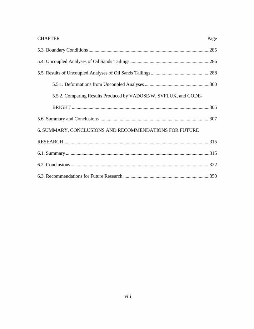
5.3. Boundary Conditions ..................................................................................................... 285
5.4. Uncoupled Analyses of Oil Sands Tailings .................................................................. 286
5.5. Results of Uncoupled Analyses of Oil Sands Tailings ................................................. 288
5.5.1. Deformations from Uncoupled Analyses ...................................................... 300
5.5.2. Comparing Results Produced by VADOSE/W, SVFLUX, and CODE-
BRIGHT ................................................................................................................... 305
5.6. Summary and Conclusions ............................................................................................ 307
6. SUMMARY, CONCLUSIONS AND RECOMMENDATIONS FOR FUTURE
RESEARCH .......................................................................................................................... 315
6.1. Summary ........................................................................................................................ 315
6.2. Conclusions .................................................................................................................... 322
6.3. Recommendations for Future Research ........................................................................ 350

ix
APPENDIX Page
A IMAGES OF SOIL SPECIMENS TESTED BY SWC-150 DEVICE ....................... 369
B RESULTS OF NUMERICAL MODELING: PROFILES OF SOILS SUCTION FOR
CORRECTED AND UNCORRECTED SWCC'S .............................................................. 385
x
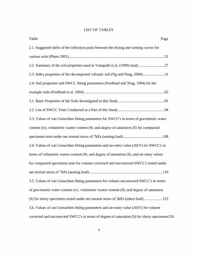
LIST OF TABLES
Table Page
2.1. Suggested shifts of the inflection point between the drying and wetting curves for
various soils (Pham 2001)....................................................................................................... 21
2.2. Summary of the soil properties used in Vanapalli et al. (1999) study ........................... 27
2.3. Index properties of the decomposed volcanic soil (Ng and Pang, 2000) ....................... 31
2.4. Soil properties and SWCC fitting parameters (Fredlund and Xing, 1994) for the
example soils (Fredlund et al. 2004) ...................................................................................... 65
3.1. Basic Properties of the Soils Investigated in this Study ................................................. 91
3.2. List of SWCC Tests Conducted as a Part of this Study .................................................. 94
3.3. Values of van Genuchten fitting parameters for SWCC's in terms of gravimetric water
content (w), volumetric waster content (θ), and degree of saturation (S) for compacted
specimens tests under net normal stress of 7kPa (seating load) .......................................... 108
3.4. Values of van Genuchten fitting parameters and air-entry value (AEV) for SWCC's in
terms of volumetric waster content (θ), and degree of saturation (S), and air-entry values
for compacted specimens tests for volume corrected and uncorrected SWCC's tested under
net normal stress of 7kPa (seating load) ............................................................................... 110
3.5. Values of van Genuchten fitting parameters for volume uncorrected SWCC's in terms
of gravimetric water content (w), volumetric waster content (θ), and degree of saturation
(S) for slurry specimens tested under net normal stress of 3kPa (token load) .................... 125
3.6. Values of van Genuchten fitting parameters and air-entry value (AEV) for volume
corrected and uncorrected SWCC's in terms of degree of saturation (S) for slurry specimens126
xi
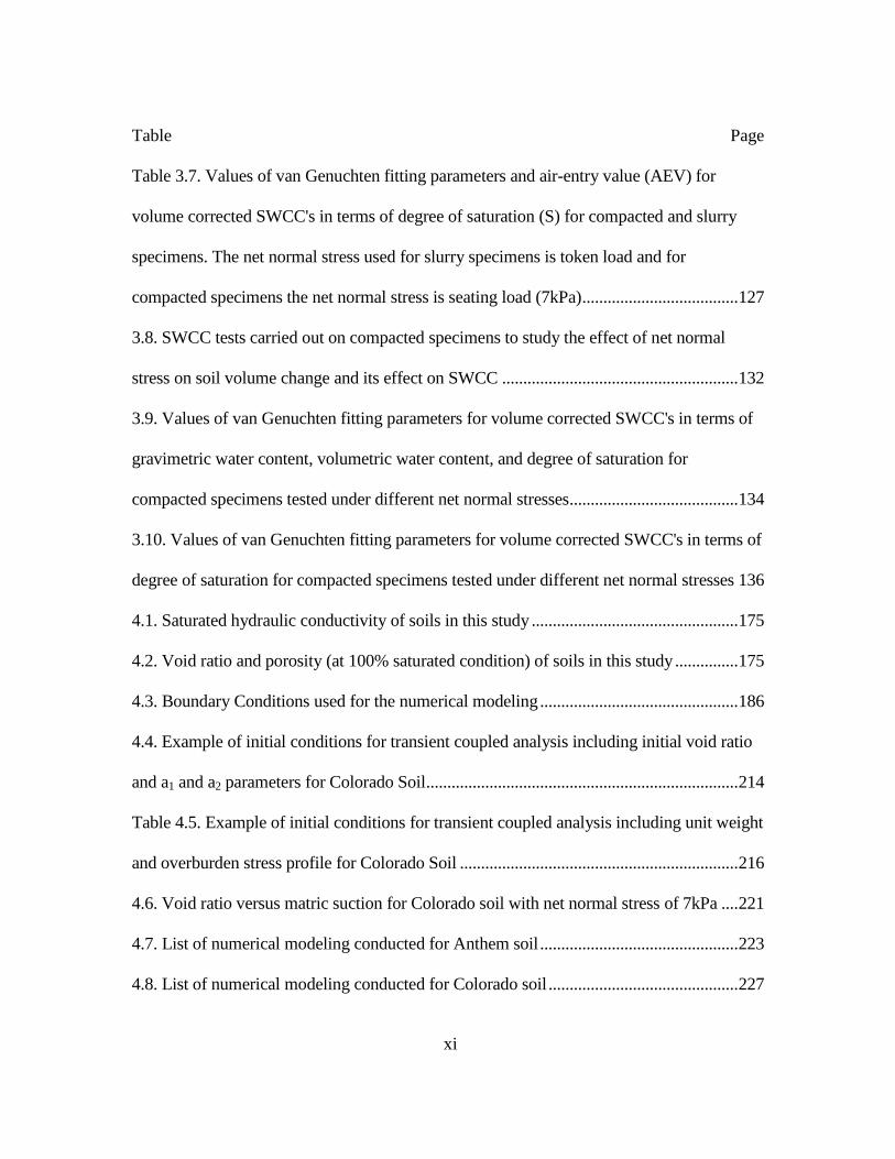
Table Page
Table 3.7. Values of van Genuchten fitting parameters and air-entry value (AEV) for
volume corrected SWCC's in terms of degree of saturation (S) for compacted and slurry
specimens. The net normal stress used for slurry specimens is token load and for
compacted specimens the net normal stress is seating load (7kPa) ..................................... 127
3.8. SWCC tests carried out on compacted specimens to study the effect of net normal
stress on soil volume change and its effect on SWCC ........................................................ 132
3.9. Values of van Genuchten fitting parameters for volume corrected SWCC's in terms of
gravimetric water content, volumetric water content, and degree of saturation for
compacted specimens tested under different net normal stresses ........................................ 134
3.10. Values of van Genuchten fitting parameters for volume corrected SWCC's in terms of
degree of saturation for compacted specimens tested under different net normal stresses 136
4.1. Saturated hydraulic conductivity of soils in this study ................................................. 175
4.2. Void ratio and porosity (at 100% saturated condition) of soils in this study ............... 175
4.3. Boundary Conditions used for the numerical modeling ............................................... 186
4.4. Example of initial conditions for transient coupled analysis including initial void ratio
and a1 and a2 parameters for Colorado Soil .......................................................................... 214
Table 4.5. Example of initial conditions for transient coupled analysis including unit weight
and overburden stress profile for Colorado Soil .................................................................. 216
4.6. Void ratio versus matric suction for Colorado soil with net normal stress of 7kPa .... 221
4.7. List of numerical modeling conducted for Anthem soil ............................................... 223
4.8. List of numerical modeling conducted for Colorado soil ............................................. 227
xii
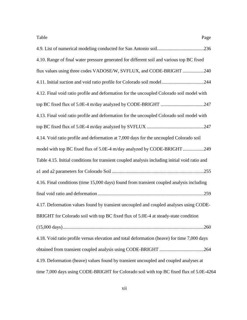
Table Page
4.9. List of numerical modeling conducted for San Antonio soil........................................ 236
4.10. Range of final water pressure generated for different soil and various top BC fixed
flux values using three codes VADOSE/W, SVFLUX, and CODE-BRIGHT .................. 240
4.11. Initial suction and void ratio profile for Colorado soil model .................................... 244
4.12. Final void ratio profile and deformation for the uncoupled Colorado soil model with
top BC fixed flux of 5.0E-4 m/day analyzed by CODE-BRIGHT ..................................... 247
4.13. Final void ratio profile and deformation for the uncoupled Colorado soil model with
top BC fixed flux of 5.0E-4 m/day analyzed by SVFLUX ................................................. 247
4.14. Void ratio profile and deformation at 7,000 days for the uncoupled Colorado soil
model with top BC fixed flux of 5.0E-4 m/day analyzed by CODE-BRIGHT .................. 249
Table 4.15. Initial conditions for transient coupled analysis including initial void ratio and
a1 and a2 parameters for Colorado Soil ............................................................................... 255
4.16. Final conditions (time 15,000 days) found from transient coupled analysis including
final void ratio and deformation ........................................................................................... 259
4.17. Deformation values found by transient uncoupled and coupled analyses using CODE-
BRIGHT for Colorado soil with top BC fixed flux of 5.0E-4 at steady-state condition
(15,000 days) ......................................................................................................................... 260
4.18. Void ratio profile versus elevation and total deformation (heave) for time 7,000 days
obtained from transient coupled analysis using CODE-BRIGHT ...................................... 264
4.19. Deformation (heave) values found by transient uncoupled and coupled analyses at
time 7,000 days using CODE-BRIGHT for Colorado soil with top BC fixed flux of 5.0E-4264
xiii
Table Page
4.20. Deformation values found by transient uncoupled and coupled analyses using CODE-
BRIGHT for Colorado soil with top BC fixed flux of 5.0E-4 at steady-state condition
(15,000 days) ......................................................................................................................... 274
4.21. Deformation (heave) values found by transient uncoupled and coupled analyses at
time 7,000 days using CODE-BRIGHT for Colorado soil with top BC fixed flux of 5.0E-4274
5.1. Saturated hydraulic conductivity of Oil Sands tailings (Fredlund et al, 2011) ............ 279
5.2. Void ratio and porosity (at 100% saturated condition) of Oil Sands tailings (Fredlund et
al, 2011) ................................................................................................................................. 279
5.3. Boundary Conditions used for the modeling ................................................................ 286
5.4. List of numerical modeling conducted for oil sands tailings ........................................ 290
5.4. (Continue) List of numerical modeling conducted for Oil Sands Tailings .................. 291
5.5. Initial suction and void ratio profile for the Oil Sands tailings model ......................... 302
5.6. Final void ratio profile and deformation for the uncoupled Oil Sands tailings model
with top BC fixed flux of 1.0E-4 m/day analyzed by CODE-BRIGHT ............................. 303
5.7. Final void ratio profile and deformation for the uncoupled Oil Sands tailings model
with top BC fixed flux of 1.0E-4 m/day analyzed by SVFLUX ......................................... 305
5.8. Range of final water pressure generated for Oil Sands tailings with various top BC
fixed flux values using three codes VADOSE/W, SVFLUX, and CODE-BRIGHT ......... 306
6.1. Deformation values found by transient uncoupled and coupled analyses using CODE-
BRIGHT for Colorado soil with top BC fixed flux of 5.0E-4 at steady-state condition
(15,000 days) ......................................................................................................................... 341

xiv
Table Page
6.2. Deformation (heave) values found by transient uncoupled and coupled analyses at time
7,000 days using CODE-BRIGHT for Colorado soil with top BC fixed flux of 5.0E-4 .... 341
xv
LIST OF FIGURES
Figure Page
1.1. Oedometer pressure plate device, SWC-150 (GCTS, 2004) ....................................... 3
2.1. Zones of desaturation defined by the desorption branch of the soil-water
characteristic curve (Fredlund and Houston, 2009) .......................................................... 12
2.2. Illustration of the influence of initial state on the soil-water characteristic curve
(modified from Fredlund 2002). ....................................................................................... 13
2.3. Best-fitting curves along with the measured data points for the three soils collected
from the literature research (Pham and Fredlund, 2008) .................................................. 14
2.4. Measured data points (Fredlund 1964), best fit, and predicted SWCC's for Regina
clay .................................................................................................................................... 14
2.5. Relationships between the air-entry value and plasticity index and percentage of
coarse fraction, Bilsel (2004) ............................................................................................ 17
2.6. Definition of Variables Associated with the Soil Water Characteristic Curve along
with wetting and drying curves (modified after Fredlund, 2000 and Chao, 2007) ........... 18
2.7. Hysteresis in the unsaturated hydraulic conductivity function associated with the
drying and wetting soil-water characteristic curve (SWCC) branches. (a) Desorption and
adsorption SWCC's showing hysteresis; (b) effect of SWCC hysteresis on the unsaturated
hydraulic conductivity function (Fredlund and Houston, 2009) ....................................... 19
2.8. Schematic illustration of the slope and distance between the two boundary hysteretic
soil-water characteristic curves (Pham et al., 2003) ......................................................... 20
xvi
Figure Page
2.9. Bounding and scanning curves that comprise the drying and wetting behavior of an
unsaturated soil (Pham et al. 2003) ................................................................................... 20
2.10. Boundary drying and wetting curves for the soft and hard chalks (Pham et al., 2003)
........................................................................................................................................... 23
2.11. Boundary drying and wetting curves for the loose and dense silty sands (Pham et
al., 2003) ........................................................................................................................... 23
2.12. The SWCC for the glass beads showing hysteresis during drying and wetting cycles
(Mualem 1976).................................................................................................................. 24
2.13. Measured data points (Fleureau et al. 1995), best-fitted initial drying, and predicted
boundary wetting SWCC's for Jossigny silt ..................................................................... 24
2.14. Measured data points (Fleureau et al. 2004), best-fitted initial drying, and predicted
boundary wetting SWCC's for kaolinite. .......................................................................... 25
2.15. Measured data points (Fleureau et al. 2004) and predicted degree of saturation
SWCC's for kaolinite ........................................................................................................ 25
2.16. Hysteretic SWCC for Processed silt (Pham et al., 2003). The continuous lines are
best fit using Feng & Fredlund (1999) .............................................................................. 26
2.17. Illustration of the equivalent pressure concept (Vanapalli et al. (1999)) ................. 29
2.18. The effect of the equivalent pressure on the SWCC for specimens compacted dry of
optimum (Vanapalli et al. (1999)) .................................................................................... 29
2.19. The effect of the equivalent pressure on the SWCC at high suction values
(Vanapalli et al. (1999)) .................................................................................................... 30
xvii
Figure Page
2.20. The effect of the net normal stress on the SWCC (Ng and Pang (2000)) ................ 32
2.21. a) Gravimetric water content SWCC's measured on the Oil Sands tailings with two
initial moisture contents of 78% and 47%, b) SWCC’s plotted as the degree as saturation
versus suction for the Oil Sands tailings considering volume change of the soil (After
Fredlund and Houston, 2013) ........................................................................................... 38
2.22. a) Gravimetric water content SWCC's on Regina clay preconsolidated to 196 kPa,
b) SWCC's plotted as the degree as saturation versus suction for the Regina clay
preconsolidated to 196 kPa considering volume change of the soil (After Fredlund and
Houston, 2013) .................................................................................................................. 39
2.23. Schematic layout of modified triaxial stress path apparatus (After Ng et al., 2012) 41
2.24. Experimental kunsat for different soils (McCartney et al. 2007) ............................... 52
2.25. Comparison of the predicted relative unsaturated hydraulic conductivity using
equation by (Fredlund et al. 2004) with the measured data for Touchet silt loam (GE3)
(measured data from Brooks and Corey 1964) ................................................................. 66
2.26. Comparison of the predicted relative unsaturated hydraulic conductivity using
equation by (Fredlund et al. 2004) with the measured data for Columbia sandy loam
(measured data from Brooks and Corey 1964) ................................................................. 66
2.27. Comparison of the predicted relative unsaturated hydraulic conductivity using
equation by (Fredlund et al. 2004) with the measured data for Superstition sand
(measured data from Richards 1952) ................................................................................ 67
xviii
Figure Page
2.28. Comparison of the predicted relative unsaturated hydraulic conductivity using
equation by (Fredlund et al. 2004) with the measured data for Yolo light clay (measured
data from Moore 1939) ..................................................................................................... 67
2.29. Comparison of the predicted relative unsaturated hydraulic conductivity using
equation by (Fredlund et al. 2004) with the measured data for Guelph loam (measured
data from Elrick and Bowman 1964) ................................................................................ 68
2.30. Comparison of the hydraulic conductivity function by van Genuchten (solid lines)
with curves obtained by applying wither Mualem theory (M; dashed line) or the Burdine
theory (B; dashed-dotted line) to the Brooks and Corey model of the SWCC (van
Genuchten, 1980) .............................................................................................................. 71
2.31. Measured (circles) and calculated curves using van Genuchten equation (solid lines)
of the soil hydraulic properties of Hygiene Sandstone (van Genuchten, 1980) ............... 72
2.32. Measured (circles) and calculated curves using van Genuchten equation (solid lines)
of the soil hydraulic properties of Touchet sit loam G.E.3 (van Genuchten, 1980) ......... 72
2.33. Measured (circles) and calculated curves using van Genuchten equation (solid
lines) of the soil hydraulic properties of sit loam G.E.3 (van Genuchten, 1980) ............. 73
2.34. Measured (circles) and calculated curves using van Genuchten equation (solid lines)
of the soil hydraulic properties of Beit Netofa Clay (van Genuchten, 1980) ................... 73
2.35. Measured (circles) and calculated curves using van Genuchten equation (solid lines)
of the soil hydraulic properties of Guelph loam (van Genuchten, 1980).......................... 74
3.1. SWC-150 Cell with pneumatic loading frame (GCTS, 2004) ................................... 86
xix
Figure Page
3.2. GCTS SWC-150 cell bottom plate (base) with mounted high air entry ceramic disk86
3.3. SWC-150 cell bottom plate (base) with grooved channel (Abbaszadeh, 2011) ........ 87
3.4. Particle Size Distribution for Anthem Soil ................................................................ 91
3.5. Particle Size Distribution for Colorado Soil .............................................................. 92
3.6. Particle Size Distribution for San Antonio Soil ......................................................... 92
3.7. Gravimetric Water Content versus Soil Suction for Compacted Specimens of
Anthem including Filter Paper Test Results ................................................................... 113
3.8. Volumetric Water Content versus Soil Suction for Compacted Specimens of Anthem,
SWCC's are corrected for soil volume change ............................................................... 113
3.9. Degree of Saturation versus Soil Suction for Compacted Specimens of Anthem,
SWCC's are corrected for soil volume change ............................................................... 114
3.10. Gravimetric Water Content versus Soil Suction for Compacted Specimens of
Colorado including Filter Paper Test Results ................................................................. 114
3.11. Volumetric Water Content versus Soil Suction for Compacted Specimens of
Colorado, SWCC's are corrected for soil volume change .............................................. 115
3.12. Degree of Saturation versus Soil Suction for Compacted Specimens of Colorado,
SWCC's are corrected for soil volume change ............................................................... 115
3.13. Gravimetric Water Content versus Soil Suction for Compacted Specimens of San
Antonio including Filter Paper Test Results ................................................................... 116
3.14. Volumetric Water Content versus Soil Suction for Compacted Specimens of San
Antonio, SWCC's are corrected for soil volume change ................................................ 116
xx
Figure Page
3.15. Degree of Saturation versus Soil Suction for Compacted Specimens of San Antonio,
SWCC's are corrected for soil volume change ............................................................... 117
3.16. Corrected and Uncorrected SWCC for Soil Volume Change in Terms of Volumetric
Water Content versus Soil Suction for Compacted Specimen of Anthem ..................... 117
3.17. Corrected and Uncorrected SWCC for Soil Volume Change in Terms of Volumetric
Water Content versus Soil Suction for Compacted Specimen of Colorado ................... 118
3.18. Corrected and Uncorrected SWCC for Soil Volume Change in Terms of Volumetric
Water Content versus Soil Suction for Compacted Specimen of San Antonio .............. 118
3.19. Corrected and Uncorrected SWCC for Soil Volume Change in Terms of Degree of
Saturation versus Soil Suction for Compacted Specimen of Anthem ............................ 119
3.20. Corrected and Uncorrected SWCC for Soil Volume Change in Terms of Degree of
Saturation versus Soil Suction for Compacted Specimen of Colorado .......................... 119
3.21. Corrected and Uncorrected SWCC for Soil Volume Change in Terms of Degree of
Saturation versus Soil Suction for Compacted Specimen of San Antonio ..................... 120
3.22. SWCC in terms of gravimetric water content for compacted specimen of Colorado
showing the method used for obtaining the AEV ........................................................... 121
3.23. SWCC in terms of volumetric water content for compacted specimen of Colorado
showing the method used for obtaining the AEV ........................................................... 122
3.24. SWCC in terms of degree of saturation for compacted specimen of Colorado
showing the method used for obtaining the AEV ........................................................... 122
3.25. Gravimetric water content versus soil suction for slurry specimen of Anthem ..... 127
xxi
Figure Page
3.26. Volumetric water content versus soil suction for slurry specimen of Anthem ...... 128
3.27. Volume corrected and uncorrected SWCC in terms of degree of saturation for slurry
specimen of Anthem ....................................................................................................... 128
3.28. Gravimetric water content versus soil suction for slurry specimen of Colorado ... 129
3.29. Volumetric water content versus soil suction for slurry specimen of Colorado .... 129
3.30. Volume corrected and uncorrected SWCC in terms of degree of saturation for slurry
specimen of Colorado ..................................................................................................... 130
3.31. Gravimetric water content versus soil suction for slurry specimen of San Antonio
......................................................................................................................................... 130
3.32. Volumetric water content versus soil suction for slurry specimens of San Antonio
......................................................................................................................................... 131
3.33. Volume corrected and uncorrected SWCC in terms of degree of saturation for slurry
specimen of San Antonio ................................................................................................ 131
3.34. Drying and wetting SWCC in terms of gravimetric water content for Anthem soil
(swell pressure: 115 kPa) under net normal stress of 7kPa ............................................ 136
3.35. Drying and wetting SWCC in terms of volumetric water content for Anthem soil
(swell pressure: 115 kPa) under net normal stress of 7kPa ............................................ 137
3.36. Drying and wetting SWCC in terms of degree of saturation for Anthem soil (swell
pressure: 115 kPa) under net normal stress of 7kPa ....................................................... 137
3.37. Drying and wetting SWCC in terms of gravimetric water content for Anthem soil
(swell pressure: 115 kPa) under net normal stress equal to 23% swell pressure ............ 138

xxii
Figure Page
3.38. Drying and wetting SWCC in terms of volumetric water content for Anthem soil
(swell pressure: 115 kPa) under net normal stress equal to 23% swell pressure ............ 138
3.39. Drying and wetting SWCC in terms of degree of saturation for Anthem soil (swell
pressure: 115 kPa) under net normal stress equal to 23% swell pressure ....................... 139
3.40. Drying and wetting SWCC in terms of gravimetric water content for Anthem soil
(swell pressure: 115 kPa) under net normal stress equal to 46% swell pressure ............ 139
3.41. Drying and wetting SWCC in terms of volumetric water content for Anthem soil
(swell pressure: 115 kPa) under net normal stress equal to 46% swell pressure ............ 140
3.42. Drying and wetting SWCC in terms of degree of saturation for Anthem soil (swell
pressure: 115 kPa) under net normal stress equal to 46% swell pressure ....................... 140
3.43. Drying SWCC in terms of degree of saturation for Anthem soil (swell pressure: 115
kPa) under various net normal stresses. Notice larger values of "a" parameter for tests
under higher net normal stress ........................................................................................ 141
3.44. Drying and wetting SWCC in terms of gravimetric water content for Colorado soil
(swell pressure: 250 kPa) under net normal stress of 7kPa ............................................ 141
3.45. Drying and wetting SWCC in terms of volumetric water content for Colorado soil
(swell pressure: 250 kPa) under net normal stress of 7kPa ............................................ 142
3.46. Drying and wetting SWCC in terms of degree of saturation for Colorado soil (swell
pressure: 250 kPa) under net normal stress of 7kPa ....................................................... 142
3.47. Drying and wetting SWCC in terms of gravimetric water content for Colorado soil
(swell pressure: 250 kPa) under net normal stress equal to 21% swell pressure ............ 143

xxiii
Figure Page
3.48. Drying and wetting SWCC in terms of volumetric water content for Colorado soil
(swell pressure: 250 kPa) under net normal stress equal to 21% swell pressure ............ 143
3.49. Drying and wetting SWCC in terms of degree of saturation for Colorado soil (swell
pressure: 250 kPa) under net normal stress equal to 21% swell pressure ....................... 144
3.50. Drying and wetting SWCC in terms of gravimetric water content for Colorado soil
(swell pressure: 250 kPa) under net normal stress equal to 42% swell pressure ............ 144
3.51. Drying and wetting SWCC in terms of volumetric water content for Colorado soil
(swell pressure: 250 kPa) under net normal stress equal to 42% swell pressure ............ 145
3.52. Drying and wetting SWCC in terms of degree of saturation for Colorado soil (swell
pressure: 250 kPa) under net normal stress equal to 42% swell pressure ....................... 145
3.53. Drying SWCC in terms of degree of saturation for Colorado soil (swell pressure:
250 kPa) under various net normal stresses. Notice larger values of degree of "a"
parameter for tests under higher net normal stress ......................................................... 146
3.54. Drying and wetting SWCC in terms of gravimetric water content for San Antonio
soil (swell pressure: 180 kPa) under net normal stress of 7kPa ...................................... 146
3.55. Drying and wetting SWCC in terms of volumetric water content for San Antonio
soil (swell pressure: 180 kPa) under net normal stress of 7kPa ...................................... 147
3.56. Drying and wetting SWCC in terms of degree of saturation for San Antonio soil
(swell pressure: 180 kPa) under net normal stress of 7kPa ............................................ 147
3.57. Drying and wetting SWCC in terms of gravimetric water content for San Antonio
soil (swell pressure: 180 kPa) under net normal stress equal to 27% swell pressure ..... 148
xxiv
Figure Page
3.58. Drying and wetting SWCC in terms of volumetric water content for San Antonio
soil (swell pressure: 180 kPa) under net normal stress equal to 27% swell pressure ..... 148
3.59. Drying and wetting SWCC in terms of degree of saturation for San Antonio soil
(swell pressure: 180 kPa) under net normal stress equal to 27% swell pressure ............ 149
3.60. Drying and wetting SWCC in terms of gravimetric water content for San Antonio
soil (swell pressure: 180 kPa) under net normal stress equal to 54% swell pressure ..... 149
3.61. Drying and wetting SWCC in terms of volumetric water content for San Antonio
soil (swell pressure: 180 kPa) under net normal stress equal to 54% swell pressure ..... 150
3.62. Drying and wetting (corrected and uncorrected) SWCC in terms of degree of
saturation for San Antonio soil (swell pressure: 180 kPa) under net normal stress equal to
54% swell pressure ......................................................................................................... 150
3.63. Drying SWCC in terms of degree of saturation for San Antonio soil (swell pressure:
180 kPa) under various net normal stresses. Notice larger values of "a" parameter for tests
under higher net normal stress ........................................................................................ 151
3.64. Drying SWCC, 200kPa suction, 7 kPa net normal stress (seating load), Anthem soil
......................................................................................................................................... 152
3.65. Drying SWCC, 1300kPa suction, 7 kPa net normal stress (seating load), Anthem
soil ................................................................................................................................... 152
3.66. Drying SWCC, 400kPa suction, 26 kPa net normal stress (23% swell pressure),
Anthem soil. Notice that almost no radial shrinkage has occurred, although there is some
vertical displacement ...................................................................................................... 153
xxv
Figure Page
3.67. Anthem specimen equilibrated at suction of 1330kPa under net normal stress of
53kPa (46% Swell Pressure). Note the minimal radial shrinkage in the specimen,
although there is some vertical displacement ................................................................. 153
3.68. Drying SWCC, 400kPa suction, 7 kPa net normal stress (seating load), San Antonio
soil ................................................................................................................................... 154
3.69. Drying SWCC, 1300kPa suction, 98 kPa net normal stress (54% swell pressure),
San Antonio soil (Notice minimal radial shrinkage and some vertical deformation
compared to net normal stress of 7kPa) .......................................................................... 154
3.70. Drying SWCC, 400kPa suction, 105 kPa net normal stress (42% Swell Pressure),
Colorado soil (Notice that almost no radial shrinkage has occurred, although there is
some vertical displacement) ............................................................................................ 155
3.71. SWCC in terms of degree of saturation for compacted specimen of Colorado
showing the method used for obtaining the AEV ........................................................... 157
3.72. Volume corrected and uncorrected SWCC in terms of degree of saturation for slurry
specimen of San Antonio ................................................................................................ 159
3.73. Drying SWCC in terms of degree of saturation for Colorado soil (swell pressure:
250 kPa) under various net normal stresses. Notice larger values of degree of "a"
parameter for tests under higher net normal stress ......................................................... 160
4.1. Pressure contours and flow vectors for a 3 kPa AEV material (GEO-SLOPE
International Ltd., 2012) ................................................................................................. 163

xxvi
Figure Page
4.2. Pressure contours and flow vectors for a 10 kPa AEV material (GEO-SLOPE
International Ltd., 2012) ................................................................................................. 164
4.3. Geometry of the Model in VADOSE/W (Dimensions are in meters) ..................... 174
4.4. SWCC of Anthem soil in terms of volumetric water content, corrected and
uncorrected for soil volume change used in VADOSE/W and SVFLUX ...................... 180
4.5. SWCC of Anthem soil in terms of degree of saturation, corrected and uncorrected for
soil volume change used in CODE-BRIGHT ................................................................. 180
4.6. kunsat function of Anthem soil estimated by SVFLUX and CODE-BRIGHT .......... 181
4.7. SWCC of Colorado soil in terms of volumetric water content, corrected and
uncorrected for soil volume change used in VADOSE/W and SVFLUX showing the
method used for obtaining the AEV ............................................................................... 182
4.8. SWCC of Colorado soil in terms of degree of saturation, corrected and uncorrected
for soil volume change used in CODE-BRIGHT showing the method used for obtaining
the AEV .......................................................................................................................... 183
4.9. kunsat function of Colorado soil estimated by SVFLUX and CODE-BRIGHT ........ 183
4.10. SWCC of San Antonio soil in terms of volumetric water content, corrected and
uncorrected for soil volume change used in VADOSE/W and SVFLUX ...................... 184
4.11. SWCC of San Antonio soil in terms of degree of saturation, corrected and
uncorrected for soil volume change used in CODE-BRIGHT ....................................... 185
4.12. kunsat function of San Antonio soil estimated by SVFLUX and CODE-BRIGHT . 185
xxvii
Figure Page
4.13. An example of initial suction versus elevation profile used for majority of coupled
and uncoupled transient modeling .................................................................................. 213
4.14. Unit Weight versus suction for Colorado soil compacted specimens obtained from
SWCC laboratory test ..................................................................................................... 215
4.15. Normal compression line (ncl) and unloading-reloading line (url) in void ratio:
ln(p')) compression plane (Muir Wood, 1991) ............................................................... 218
4.16. Results of one-dimensional compression test in oedometer interpreted in terms of
compression index cC and swelling index sC (Muir Wood, 1991) .............................. 218
4.17. Transient analysis on Anthem soil with SWCC uncorrected for volume change
(AEV= 15kPa) and top fixed flux of 1.0e-3 m/day using CODE-BRIGHT ................... 224
4.18. Transient analysis on Anthem soil with SWCC corrected for volume change (AEV=
50kPa) and top fixed flux of 1.0e-3 m/day using CODE-BRIGHT ............................... 224
4.19. Water pressure versus elevation at time 4,000days (11 years) for Anthem soil with
SWCC corrected (AEV= 50kPa) and uncorrected (AEV= 15kPa) for volume change and
top fixed flux of 1.0E-3 m/day using CODE-BRIGHT .................................................. 225
4.20. Water pressure versus elevation at steady-state condition (time: 7,000 days) for
Anthem soil with SWCC corrected (AEV= 50kPa) and uncorrected (AEV= 15kPa) for
volume change and top fixed flux of 1.0E-3 m/day using CODE-BRIGHT .................. 225
4.21. Transient analysis on Colorado soil with SWCC uncorrected for volume change
(AEV= 60kPa) and top fixed flux of 5.0e-4 m/day using CODE-BRIGHT ................... 228
xxviii
Figure Page
4.22. Transient analysis on Colorado soil with SWCC corrected for volume change
(AEV= 90kPa) and top fixed flux of 5.0e-4 m/day using CODE-BRIGHT ................... 228
4.23. Water pressure versus elevation at time 7,000days (19 years) for Colorado soil with
SWCC corrected (AEV= 90kPa) and uncorrected (AEV= 60kPa) for volume change and
top fixed flux of 5.0e-4 m/day using CODE-BRIGHT................................................... 229
4.24. Water pressure versus elevation at steady-state condition (time: 15,000 days) for
Colorado soil with SWCC corrected (AEV= 90kPa) and uncorrected (AEV= 60kPa) for
volume change and top fixed flux of 5.0e-4 m/day using CODE-BRIGHT .................. 229
4.25. Transient analysis on Colorado soil with SWCC uncorrected for volume change
(AEV= 50kPa) and top fixed flux of 1.0e-3 m/day using SVFLUX .............................. 230
4.26. Transient analysis on Colorado soil with SWCC corrected for volume change
(AEV= 80kPa) and top fixed flux of 1.0e-3 m/day using SVFLUX .............................. 230
4.27. Water pressure versus elevation at time 400,000days (1095 years) for Colorado soil
with SWCC corrected (AEV= 90kPa) and uncorrected (AEV= 60kPa) for volume change
and top fixed flux of -1.0E-6 m/day (evaporation) using CODE-BRIGHT ................... 231
4.28. An example of initial suction versus elevation profile showing higher suction values
used for uncoupled transient modeling of Colorado soil ................................................ 232
4.29. Water pressure versus elevation at time 32,000days for Colorado soil with SWCC
corrected (AEV= 90kPa) and uncorrected (AEV= 60kPa) for volume change and top
fixed flux of 1.0E-4 m/day using CODE-BRIGHT ........................................................ 233

xxix
Figure Page
4.30. Water pressure versus elevation at time 60,000days for Colorado soil with SWCC
corrected (AEV= 90kPa) and uncorrected (AEV= 60kPa) for volume change and top
fixed flux of 1.0E-4 m/day using CODE-BRIGHT ........................................................ 234
4.31. Water pressure versus elevation at time 90,000days (steady-state) for Colorado soil
with SWCC corrected (AEV= 90kPa) and uncorrected (AEV= 60kPa) for volume change
and top fixed flux of 1.0E-4 m/day using CODE-BRIGHT ........................................... 234
4.32. Transient analysis on San Antonio soil with SWCC uncorrected for volume change
(AEV= 30kPa) and top fixed flux of 5.0e-4 m/day using CODE-BRIGHT ................... 237
4.33. Transient analysis on San Antonio soil with SWCC corrected for volume change
(AEV= 70kPa) and top fixed flux of 5.0e-4 m/day using CODE-BRIGHT ................... 237
4.34. Water pressure versus elevation at time 6,000 days (16 years) for San Antonio soil
with SWCC corrected (AEV= 70kPa) and uncorrected (AEV= 30kPa) for volume change
and top fixed flux of 5.0e-4 m/day using CODE-BRIGHT ............................................ 238
4.35. Water pressure versus elevation at time 10,000 days (27 years) for San Antonio soil
with SWCC corrected (AEV= 70kPa) and uncorrected (AEV= 30kPa) for volume change
and top fixed flux of 5.0e-4 m/day using CODE-BRIGHT ............................................ 238
4.36. Water pressure versus elevation at steady-state condition for San Antonio soil with
SWCC corrected (AEV= 70kPa) and uncorrected (AEV= 30kPa) for volume change and
top fixed flux of 5.0e-4 m/day using CODE-BRIGHT................................................... 239
xxx
Figure Page
4.37. Water pressure versus elevation at steady-state condition for Colorado soil with
SWCC corrected and uncorrected for volume change and top fixed flux of 5.0e-4 m/day
using SVFLUX, VADOSE/W, and CODE-BRIGHT .................................................... 241
4.38. Water pressure versus elevation at steady-state condition for San Antonio soil with
SWCC corrected and uncorrected for volume change and top fixed flux of 5.0e-4 m/day
using SVFLUX, VADOSE/W, and CODE-BRIGHT .................................................... 242
4.39. Suction compression curve for Colorado soil compacted specimens obtained from
SWCC laboratory test ..................................................................................................... 243
4.40. Water pressure versus elevation at steady-state condition for Colorado soil with
SWCC corrected and uncorrected for volume change and top fixed flux of 5.0e-4 m/day
using SVFLUX, VADOSE/W, and CODE-BRIGHT. The soil profile has become fully
saturated in this case ....................................................................................................... 243
4.41. Water pressure versus elevation at 7,000 days for Colorado soil with SWCC
corrected (AEV= 90kPa) and uncorrected (AEV= 60kPa) for volume change and top
fixed flux of 5.0e-4 m/day using CODE-BRIGHT. The soil profile has not become fully
saturated at the time of 7,000 days .................................................................................. 248
4.42. Initial suction versus elevation profile used for coupled and uncoupled transient
modeling ......................................................................................................................... 250
4.43. Suction compression curve for Colorado soil compacted specimens obtained from
SWCC laboratory test ..................................................................................................... 251
xxxi
Figure Page
4.44. Unit Weight versus suction for Colorado soil compacted specimens obtained from
SWCC laboratory test ..................................................................................................... 252
4.45. Sub-layering the soil column for defining initial void ratio more accurately to each
sub-layer .......................................................................................................................... 254
4.46. Transient coupled flow-deformation analysis on Colorado soil with SWCC
uncorrected for volume change (AEV= 60kPa) and top fixed flux of 5.0e-4 m/day using
CODE-BRIGHT ............................................................................................................. 255
4.47. Transient coupled flow-deformation analysis on Colorado soil with SWCC
corrected for volume change (AEV= 90kPa) and top fixed flux of 5.0e-4 m/day using
CODE-BRIGHT ............................................................................................................. 256
4.48. Water pressure versus elevation at steady-state condition for coupled flow-
deformation analysis on Colorado soil with SWCC corrected (AEV= 90kPa) and
uncorrected (AEV= 60kPa) for volume change and top fixed flux of 5.0e-4 m/day using
CODE-BRIGHT ............................................................................................................. 256
4.49. Transient coupled flow-deformation analysis on Colorado soil with SWCC
uncorrected for volume change (AEV= 60kPa) and top fixed flux of 5.0e-4 m/day using
CODE-BRIGHT ............................................................................................................. 257
4.50. Transient coupled flow-deformation analysis on Colorado soil with SWCC
corrected for volume change (AEV= 90kPa) and top fixed flux of 5.0e-4 m/day using
CODE-BRIGHT ............................................................................................................. 258
xxxii
Figure Page
4.51. Void ratio versus elevation at steady-state condition for coupled flow-deformation
analysis on Colorado soil with SWCC corrected (AEV= 90kPa) and uncorrected (AEV=
60kPa) for volume change and top fixed flux of 5.0e-4 m/day using CODE-BRIGHT 258
4.52. Water pressure versus elevation at 7,000 days for Colorado soil with SWCC
corrected (AEV= 90kPa) and uncorrected (AEV= 60kPa) for volume change and top
fixed flux of 5.0e-4 m/day using CODE-BRIGHT. The soil profile has not become fully
saturated at the time of 7,000 days .................................................................................. 262
4.53. Void ratio versus elevation at 7,000 days for Colorado soil with SWCC corrected
(AEV= 90kPa) and uncorrected (AEV= 60kPa) for volume change and top fixed flux of
5.0e-4 m/day using CODE-BRIGHT. The soil profile has not become fully saturated at
the time of 7,000 days ..................................................................................................... 262
4.54. Water pressure versus elevation at steady-state condition (time: 15,000 days) for
Colorado soil with SWCC corrected (AEV= 90kPa) and uncorrected (AEV= 60kPa) for
volume change and top fixed flux of 5.0e-4 m/day using CODE-BRIGHT .................. 267
4.55. Water pressure versus elevation at time 7,000days (19 years) for Colorado soil with
SWCC corrected (AEV= 90kPa) and uncorrected (AEV= 60kPa) for volume change and
top fixed flux of 5.0e-4 m/day using CODE-BRIGHT................................................... 269
4.56. Water pressure versus elevation at time 400,000days (1095 years) for Colorado soil
with SWCC corrected (AEV= 90kPa) and uncorrected (AEV= 60kPa) for volume change
and top fixed flux of -1.0E-6 m/day (evaporation) using CODE-BRIGHT ................... 270
xxxiii
Figure Page
4.57. Water pressure versus elevation at time 60,000days for Colorado soil with SWCC
corrected (AEV= 90kPa) and uncorrected (AEV= 60kPa) for volume change and top
fixed flux of 1.0E-4 m/day using CODE-BRIGHT ........................................................ 271
4.58. Water pressure versus elevation at time 90,000days (steady-state) for Colorado soil
with SWCC corrected (AEV= 90kPa) and uncorrected (AEV= 60kPa) for volume change
and top fixed flux of 1.0E-4 m/day using CODE-BRIGHT ........................................... 272
4.59. Water pressure versus elevation at steady-state condition for Colorado soil with
SWCC corrected and uncorrected for volume change and top fixed flux of 5.0e-4 m/day
using SVFLUX, VADOSE/W, and CODE-BRIGHT .................................................... 273
5.1. SWCC of Oil Sands tailings in terms of volumetric water content used in
VADOSE/W and SVFLUX ............................................................................................ 284
5.2. SWCC of Oil Sands tailings in terms of degree of saturation used in CODE-BRIGHT
......................................................................................................................................... 284
5.3. kunsat function of Oil Sands tailings estimated by SVFLUX and CODE-BRIGHT . 285
5.4. Initial suction versus elevation profile used for coupled and uncoupled transient
modeling ......................................................................................................................... 288
5.5. Transient analyses on Oil Sands tailings with SWCC uncorrected for volume change
and top fixed flux of 2.0e-4 m/day using SVFLUX ....................................................... 292
5.6. Transient analyses on Oil Sands tailings with SWCC corrected for volume change
and top fixed flux of 2.0e-4 m/day using SVFLUX ....................................................... 292
xxxiv
Figure Page
5.7. Water pressure versus elevation at steady-state condition for Oil Sands tailings with
SWCC corrected and uncorrected for volume change and top fixed flux of 2.0e-4 m/day
using SVFLUX ............................................................................................................... 293
5.8. Transient analyses on Oil Sands tailings with SWCC uncorrected for volume change
and top fixed flux of 1.0e-4 m/day using CODE-BRIGHT ............................................ 295
5.9. Transient analyses on Oil Sands tailings with SWCC corrected for volume change
and top fixed flux of 1.0e-4 m/day using CODE-BRIGHT ............................................ 295
5.10. Water pressure versus elevation at time 60,000 days (164 years) for Oil Sands
tailings with SWCC corrected and uncorrected for volume change and top fixed flux of
1.0e-4 m/day using CODE-BRIGHT .............................................................................. 296
5.11. Water pressure versus elevation at steady-state condition (104,000 days) for Oil
Sands tailings with SWCC corrected and uncorrected for volume change and top fixed
flux of 1.0e-4 m/day using CODE-BRIGHT .................................................................. 297
5.12. Water pressure versus elevation at steady-state condition for Oil Sands tailings with
SWCC corrected and uncorrected for volume change and top fixed head of 1m using
SVFLUX ......................................................................................................................... 298
5.13. Water pressure versus depth at steady-state condition for oil sands tailings with
SWCC corrected and uncorrected for volume change and top fixed flux of -1.0E-6 m/day
(evaporation) using VADOSE/W ................................................................................... 299
xxxv
Figure Page
5.14. Water pressure versus depth at steady-state condition for oil sands tailings with
SWCC corrected and uncorrected for volume change and top fixed flux of -1.0E-7 m/day
(evaporation) using VADOSE/W ................................................................................... 299
5.15. Suction compression curve for Oil Sands tailings (Fredlund and Houston, 2013, and
Fredlund et al., 2011) ...................................................................................................... 301
5.16. Water pressure versus elevation at steady-state condition for Oil Sands tailings with
SWCC corrected and uncorrected for volume change and top fixed flux of 1.0e-4 m/day
using SVFLUX, VADOSE/W, and CODE-BRIGHT .................................................... 301
5.17. Water pressure versus elevation at steady-state condition for Oil Sands tailings with
SWCC corrected and uncorrected for volume change and top fixed flux of 1.0e-4 m/day
using SVFLUX, VADOSE/W, and CODE-BRIGHT .................................................... 307
5.18. Water pressure versus elevation at steady-state condition (104,000 days) for Oil
Sands tailings with SWCC corrected and uncorrected for volume change and top fixed
flux of 1.0e-4 m/day using CODE-BRIGHT .................................................................. 311
5.19. Water pressure versus elevation at time 60,000 days (164 years) for Oil Sands
tailings with SWCC corrected and uncorrected for volume change and top fixed flux of
1.0e-4 m/day using CODE-BRIGHT .............................................................................. 312
5.20. Water pressure versus depth at steady-state condition for oil sands tailings with
SWCC corrected and uncorrected for volume change and top fixed flux of -1.0E-7 m/day
(evaporation) using VADOSE/W ................................................................................... 313
xxxvi
Figure Page
6.1. Typical impact of volume change correction on shape of the SWCC - example here
is for compacted specimen of Colorado.......................................................................... 325
6.2. (a) Example of volume corrected and uncorrected SWCC's in terms of degree of
saturation for slurry specimen and the corresponding van Genuchten parameters (for San
Antonio soil), and (b) Example of volume corrected SWCC's in terms of degree of
saturation for compacted and slurry specimens and the corresponding van Genuchten
parameters (for San Antonio soil) ................................................................................... 325
6.3. Typical effect of net normal stress on compacted expansive soils SWCC’s – shown
here are Drying SWCC's for Colorado soil (swell pressure: 250 kPa) under various net
normal stresses. Notice larger values of "a" parameter for tests under higher net normal
stress ................................................................................................................................ 330
6.4. Example profile of soils suction for corrected and uncorrected SWCC. Water
pressure versus elevation at steady-state condition (time: 15,000 days) for Colorado soil
with SWCC corrected (AEV= 90kPa) and uncorrected (AEV= 60kPa) for volume change
and top fixed flux of 5.0e-4 m/day using CODE-BRIGHT ............................................ 333
6.5. Example profile of soils suction for corrected and uncorrected SWCC. Water
pressure versus elevation profile at time 7,000days (19 years) for Colorado soil with
SWCC corrected (AEV= 90kPa) and uncorrected (AEV= 60kPa) for volume change and
top fixed flux of 5.0e-4 m/day using CODE-BRIGHT................................................... 335
xxxvii
Figure Page
6.6. Example profile of soils suction for corrected and uncorrected SWCC. Water
pressure versus elevation profile at time 400,000days (1095 years) for Colorado soil with
SWCC corrected (AEV= 90kPa) and uncorrected (AEV= 60kPa) for volume change and
top fixed flux of -1.0E-6 m/day (evaporation) using CODE-BRIGHT .......................... 336
6.7. Example profile of soils suction for corrected and uncorrected SWCC. Water
pressure versus elevation profile at time 60,000days for Colorado soil with SWCC
corrected (AEV= 90kPa) and uncorrected (AEV= 60kPa) for volume change and top
fixed flux of 1.0E-4 m/day using CODE-BRIGHT ........................................................ 337
6.8. Example profile of soils suction for corrected and uncorrected SWCC. Water
pressure versus elevation profile at time 90,000days (steady-state) for Colorado soil with
SWCC corrected (AEV= 90kPa) and uncorrected (AEV= 60kPa) for volume change and
top fixed flux of 1.0E-4 m/day using CODE-BRIGHT .................................................. 338
6.9. Example profile of soils suction for corrected and uncorrected SWCC. Water
pressure versus elevation profile at steady-state condition for Colorado soil with SWCC
corrected and uncorrected for volume change and top fixed flux of 5.0e-4 m/day using
SVFLUX, VADOSE/W, and CODE-BRIGHT .............................................................. 340
6.10. Example profile of soils suction for corrected and uncorrected SWCC. Water
pressure versus elevation profile at steady-state condition (104,000 days) for Oil Sands
tailings with SWCC corrected and uncorrected for volume change and top fixed flux of
1.0e-4 m/day using CODE-BRIGHT .............................................................................. 346
xxxviii
Figure Page
6.11. Example profile of soils suction for corrected and uncorrected SWCC. Water
pressure versus elevation profile at time 60,000 days (164 years) for Oil Sands tailings
with SWCC corrected and uncorrected for volume change and top fixed flux of 1.0e-4
m/day using CODE-BRIGHT ......................................................................................... 348
6.12. Example profile of soils suction for corrected and uncorrected SWCC. Water
pressure profile versus depth at steady-state condition for oil sands tailings with SWCC
corrected and uncorrected for volume change and top fixed flux of -1.0E-7 m/day
(evaporation) using VADOSE/W ................................................................................... 349
A.1. Slurry Specimen of Anthem on High Air Entry Ceramic Stone of SWCC Cell
Equilibrated at 25kPa Suction under Token Load .......................................................... 370
A.2. Slurry Specimen of Anthem on High Air Entry Ceramic Stone of SWCC Cell
Equilibrated at 50kPa Suction under Token Load .......................................................... 370
A.3. Slurry Specimen of Anthem on High Air Entry Ceramic Stone of SWCC Cell
Equilibrated at 100kPa Suction under Token Load ........................................................ 371
A.4. Slurry Specimen of Anthem on High Air Entry Ceramic Stone of SWCC Cell
Equilibrated at 200kPa Suction under Token Load ........................................................ 371
A.5. Slurry Specimen of Anthem on High Air Entry Ceramic Stone of SWCC Cell
Equilibrated at 400kPa Suction under Token Load ........................................................ 372
A.6. Slurry Specimen of Anthem on High Air Entry Ceramic Stone of SWCC Cell
Equilibrated at 1,250kPa Suction under Token Load ..................................................... 372
xxxix
Figure Page
A.7. Slurry Specimen of Colorado on High Air Entry Ceramic Stone of SWCC Cell
Equilibrated at 25kPa Suction under Token Load .......................................................... 373
A.8. Slurry Specimen of Colorado on High Air Entry Ceramic Stone of SWCC Cell
Equilibrated at 50kPa Suction under Token Load .......................................................... 373
A.9. Slurry Specimen of Colorado on High Air Entry Ceramic Stone of SWCC Cell
Equilibrated at 100kPa Suction under Token Load ........................................................ 374
A.10. Slurry Specimen of Colorado on High Air Entry Ceramic Stone of SWCC Cell
Equilibrated at 200kPa Suction under Token Load ........................................................ 374
A.11. Slurry Specimen of Colorado on High Air Entry Ceramic Stone of SWCC Cell
Equilibrated at 400kPa Suction under Token Load ........................................................ 375
A.12. Slurry Specimen of San Antonio on High Air Entry Ceramic Stone of SWCC Cell
Equilibrated at 25kPa Suction under Token Load .......................................................... 375
A.13. Slurry Specimen of San Antonio on High Air Entry Ceramic Stone of SWCC Cell
Equilibrated at 50kPa Suction under Token Load .......................................................... 376
A.14. Slurry Specimen of San Antonio on High Air Entry Ceramic Stone of SWCC Cell
Equilibrated at 100kPa Suction under Token Load ........................................................ 376
A.15. Slurry Specimen of San Antonio on High Air Entry Ceramic Stone of SWCC Cell
Equilibrated at 200kPa Suction under Token Load ........................................................ 377
A.16. Slurry Specimen of San Antonio on High Air Entry Ceramic Stone of SWCC Cell
Equilibrated at 400kPa Suction under Token Load ........................................................ 377
xl
Figure Page
A.17. Compacted Specimen of Anthem on High Air Entry Ceramic Stone of SWCC Cell
Equilibrated at 100kPa Suction under Seating Load ...................................................... 378
A.18. Compacted Specimen of Anthem on High Air Entry Ceramic Stone of SWCC Cell
Equilibrated at 400kPa Suction under Seating Load ...................................................... 378
A.19. Compacted Specimen of Anthem on High Air Entry Ceramic Stone of SWCC Cell
Equilibrated at 1,300kPa Suction under Seating Load ................................................... 379
A.20. Compacted Specimen of Colorado on High Air Entry Ceramic Stone of SWCC
Cell Equilibrated at 100kPa Suction under Seating Load ............................................... 379
A.21. Compacted Specimen of Colorado on High Air Entry Ceramic Stone of SWCC
Cell Equilibrated at 200kPa Suction under Seating Load ............................................... 380
A.22. Compacted Specimen of Colorado Equilibrated at 400kPa Suction under Seating
Load ................................................................................................................................ 380
A.23. Compacted Specimen of San Antonio on High Air Entry Ceramic Stone of SWCC
Cell Equilibrated at 400kPa Suction under Seating Load ............................................... 381
A.24. Compacted Specimen of San Antonio on High Air Entry Ceramic Stone of SWCC
Cell Equilibrated at 1,200kPa Suction under Seating Load ............................................ 381
A.25. Compacted Specimen of San Antonio on High Air Entry Ceramic Stone of SWCC
Cell Equilibrated at 200kPa Suction under Seating Load ............................................... 382
A.26. Compacted Specimen of San Antonio on High Air Entry Ceramic Stone of SWCC
Cell Equilibrated at 400kPa Suction under Seating Load ............................................... 382
xli
Figure Page
A.27. Application of Net Normal Pressure to Specimens and Monitoring Vertical
displacement Using Dial Gauges .................................................................................... 383
A.28. Application of Net Normal Pressure to Specimens and Monitoring Vertical
displacement Using Dial Gauges .................................................................................... 384
B.1. Water pressure versus depth at steady-state condition for oil sands tailings with
SWCC corrected and uncorrected for volume change and top fixed flux of 1.0E-5 m/day
using SVFLUX ............................................................................................................... 386
B.2. Water pressure versus depth at steady-state condition for oil sands tailings with
SWCC corrected and uncorrected for volume change and top fixed flux of 2.0E-5 m/day
using SVFLUX ............................................................................................................... 386
B.3. Water pressure versus depth at steady-state condition for oil sands tailings with
SWCC corrected and uncorrected for volume change and top fixed flux of 9.0E-5 m/day
using SVFLUX ............................................................................................................... 387
B.4. Water pressure versus depth at steady-state condition for oil sands tailings with
SWCC corrected and uncorrected for volume change and top fixed flux of 1.0E-4 m/day
using SVFLUX ............................................................................................................... 387
B.5. Water pressure versus depth at steady-state condition for oil sands tailings with
SWCC corrected and uncorrected for volume change and top fixed flux of 1.73E-4 m/day
using SVFLUX ............................................................................................................... 388
xlii
Figure Page
B.6. Water pressure versus depth at steady-state condition for oil sands tailings with
SWCC corrected and uncorrected for volume change and top fixed flux of 2.0E-4 m/day
using SVFLUX ............................................................................................................... 388
B.7. Water pressure versus depth at steady-state condition for oil sands tailings with
SWCC corrected and uncorrected for volume change and top fixed flux of 3.0E-4 m/day
using SVFLUX ............................................................................................................... 389
B.8. Water pressure versus depth at steady-state condition for oil sands tailings with
SWCC corrected and uncorrected for volume change and top fixed flux of 4.0E-4 m/day
using SVFLUX ............................................................................................................... 389
B.9. Water pressure versus depth at steady-state condition for oil sands tailings with
SWCC corrected and uncorrected for volume change and top fixed head of 1m using
SVFLUX ......................................................................................................................... 390
B.10. Water pressure versus depth at steady-state condition for oil sands tailings with
SWCC corrected and uncorrected for volume change and top fixed flux of 1.0E-5 m/day
using VADOSE/W .......................................................................................................... 390
B.11. Water pressure versus depth at steady-state condition for oil sands tailings with
SWCC corrected and uncorrected for volume change and top fixed flux of 2.0E-5 m/day
using VADOSE/W .......................................................................................................... 391
B.12. Water pressure versus depth at steady-state condition for oil sands tailings with
SWCC corrected and uncorrected for volume change and top fixed flux of 9.0E-5 m/day
using VADOSE/W .......................................................................................................... 391
xliii
Figure Page
B.13. Water pressure versus depth at steady-state condition for oil sands tailings with
SWCC corrected and uncorrected for volume change and top fixed flux of 1.0E-4 m/day
using VADOSE/W .......................................................................................................... 392
B.14. Water pressure versus depth at steady-state condition for oil sands tailings with
SWCC corrected and uncorrected for volume change and top fixed flux of 1.73E-4 m/day
using VADOSE/W .......................................................................................................... 392
B.15. Water pressure versus depth at steady-state condition for oil sands tailings with
SWCC corrected and uncorrected for volume change and top fixed flux of 2.0E-4 m/day
using VADOSE/W .......................................................................................................... 393
B.16. Water pressure versus depth at steady-state condition for oil sands tailings with
SWCC corrected and uncorrected for volume change and top fixed flux of 3.0E-4 m/day
using VADOSE/W .......................................................................................................... 393
B.17. Water pressure versus depth at steady-state condition for oil sands tailings with
SWCC corrected and uncorrected for volume change and top fixed flux of 4.0E-4 m/day
using VADOSE/W .......................................................................................................... 394
B.18. Water pressure versus depth at steady-state condition for oil sands tailings with
SWCC corrected and uncorrected for volume change and top fixed head of 1m using
VADOSE/W ................................................................................................................... 394
B.19. Water pressure versus depth at steady-state condition for oil sands tailings with
SWCC corrected and uncorrected for volume change and top fixed flux of -1.0E-5 m/day
(evaporation) using VADOSE/W ................................................................................... 395
xliv
Figure Page
B.20. Water pressure versus depth at steady-state condition for oil sands tailings with
SWCC corrected and uncorrected for volume change and top fixed flux of -1.0E-6 m/day
(evaporation) using VADOSE/W ................................................................................... 395
B.21. Water pressure versus depth at steady-state condition for oil sands tailings with
SWCC corrected and uncorrected for volume change and top fixed flux of -1.0E-7 m/day
(evaporation) using VADOSE/W ................................................................................... 396
B.22. Water pressure versus depth at steady-state condition for Anthem soil with SWCC
corrected and uncorrected for volume change and top fixed flux of 1.0E-3 m/day using
CODE-BRIGHT ............................................................................................................. 396
B.23. Water pressure versus depth at steady-state condition for Anthem soil with SWCC
corrected and uncorrected for volume change and top fixed flux of 5.0E-4 m/day using
SVFLUX ......................................................................................................................... 397
B.24. Water pressure versus depth at steady-state condition for Anthem soil with SWCC
corrected and uncorrected for volume change and top fixed flux of 1.0E-3 m/day using
SVFLUX ......................................................................................................................... 397
B.25. Water pressure versus depth at steady-state condition for Anthem soil with SWCC
corrected and uncorrected for volume change and top fixed flux of 3.0E-3 m/day using
SVFLUX ......................................................................................................................... 398
B.26. Water pressure versus depth at steady-state condition for Anthem soil with SWCC
corrected and uncorrected for volume change and top fixed flux of 7.0E-3 m/day using
SVFLUX ......................................................................................................................... 398
xlv
Figure Page
B.27. Water pressure versus depth at steady-state condition for Anthem soil with SWCC
corrected and uncorrected for volume change and top fixed flux of 8.65E-3 m/day using
SVFLUX ......................................................................................................................... 399
B.28. Water pressure versus depth at steady-state condition for Anthem soil with SWCC
corrected and uncorrected for volume change and top fixed flux of 1.0E-2 m/day using
SVFLUX ......................................................................................................................... 399
B.29. Water pressure versus depth at steady-state condition for Anthem soil with SWCC
corrected and uncorrected for volume change and top fixed head of 1m using SVFLUX
......................................................................................................................................... 400
B.30. Water pressure versus depth at steady-state condition for Colorado soil with SWCC
corrected and uncorrected for volume change and top fixed flux of 5.0E-5 m/day using
SVFLUX ......................................................................................................................... 400
B.31. Water pressure versus depth at steady-state condition for Colorado soil with SWCC
corrected and uncorrected for volume change and top fixed flux of 1.0E-4 m/day using
SVFLUX ......................................................................................................................... 401
B.32. Water pressure versus depth at steady-state condition for Colorado soil with SWCC
corrected and uncorrected for volume change and top fixed flux of 3.0E-4 m/day using
SVFLUX ......................................................................................................................... 401
B.33. Water pressure versus depth at steady-state condition for Colorado soil with SWCC
corrected and uncorrected for volume change and top fixed flux of 5.0E-4 m/day using
SVFLUX ......................................................................................................................... 402
xlvi
Figure Page
B.34. Water pressure versus depth at steady-state condition for Colorado soil with SWCC
corrected and uncorrected for volume change and top fixed flux of 7.0E-4 m/day using
SVFLUX ......................................................................................................................... 402
B.35. Water pressure versus depth at steady-state condition for Colorado soil with SWCC
corrected and uncorrected for volume change and top fixed flux of 8.64E-4 m/day using
SVFLUX ......................................................................................................................... 403
B.36. Water pressure versus depth at steady-state condition for Colorado soil with SWCC
corrected and uncorrected for volume change and top fixed flux of 1.0E-3 m/day using
SVFLUX ......................................................................................................................... 403
B.37. Water pressure versus depth at steady-state condition for Colorado soil with SWCC
corrected and uncorrected for volume change and top fixed head of 1m using SVFLUX
......................................................................................................................................... 404
B.38. Water pressure versus depth at steady-state condition for San Antonio soil with
SWCC corrected and uncorrected for volume change and top fixed flux of 5.0E-5 m/day
using SVFLUX ............................................................................................................... 404
B.39. Water pressure versus depth at steady-state condition for San Antonio soil with
SWCC corrected and uncorrected for volume change and top fixed flux of 1.0E-4 m/day
using SVFLUX ............................................................................................................... 405
B.40. Water pressure versus depth at steady-state condition for San Antonio soil with
SWCC corrected and uncorrected for volume change and top fixed flux of 3.0E-4 m/day
using SVFLUX ............................................................................................................... 405
xlvii
Figure Page
B.41. Water pressure versus depth at steady-state condition for San Antonio soil with
SWCC corrected and uncorrected for volume change and top fixed flux of 5.0E-4 m/day
using SVFLUX ............................................................................................................... 406
B.42. Water pressure versus depth at steady-state condition for San Antonio soil with
SWCC corrected and uncorrected for volume change and top fixed flux of 7.0E-4 m/day
using SVFLUX ............................................................................................................... 406
B.43. Water pressure versus depth at steady-state condition for San Antonio soil with
SWCC corrected and uncorrected for volume change and top fixed flux of 8.64E-4 m/day
using SVFLUX ............................................................................................................... 407
B.44. Water pressure versus depth at steady-state condition for San Antonio soil with
SWCC corrected and uncorrected for volume change and top fixed flux of 1.0E-3 m/day
using SVFLUX ............................................................................................................... 407
B.45. Water pressure versus depth at steady-state condition for San Antonio soil with
SWCC corrected and uncorrected for volume change and top fixed head of 1m using
SVFLUX ......................................................................................................................... 408
1
Chapter 1
INTRODUCTION
1.1. Background
Unsaturated soil mechanics has gradually become a part of geotechnical
engineering practice, particularly in the areas of expansive and collapsible soils and
geoenvironmental engineering. The Soil Water Characteristic Curve (SWCC) which is
often referred to as the soil water retention curve is one of the main parameters which has
been developed and used by researchers for many years in the study of unsaturated soils.
The SWCC has been used in the estimation of unsaturated soil property functions, in
general, and has been used for decades for estimation of the unsaturated hydraulic
conductivity function (Fredlund et al. 2000, van Genuchten and Mualem, 1980).
The SWCC defines the amount of water in a soil for different values of soil
suction. The amount of water in the soil is commonly defined in one of several ways.
Three common variables used to define the amount of water in the soil are: gravimetric
water content, w, volumetric water content, θ, and degree of saturation, S. SWCC’s in
terms of all three measures of soil water content are used to obtain information such as
the air-entry value and residual suction, and when the soil does not undergo volume
change (e.g., sands), should yield similar values (Fredlund, 2006).
The SWCC can be used to estimate the unsaturated hydraulic conductivity of a
soil. The drying SWCC is generally measured in the laboratory and therefore, the
hydraulic conductivity function is typically determined based on the drying curve.
2
However, the hydraulic conductivity function for the wetting curve can be estimated
based on measured or estimated hysteresis loops (Pham et al, 2003).
SWCC's have been established in agriculture-related disciplines for many years.
A number of devices have been developed for applying a wide range of soil suction
values (Fredlund, 2006). Typical pressure plate apparatuses and their range of suction
application are: Tempe cells (100 kPa) (Reginato and van Bavel 1962); volumetric
pressure plate (200 kPa); and large pressure plate (500 and 1,500 kPa) (Fredlund and
Rahardjo 1993). ASTM standard (ASTM 2003 Standard D-6836-02) provides a detailed
description for the determination of the soil water characteristic curves using several
testing procedures.
One of the most common devices that has been used for determining SWCC's in
geotechnical engineering is the oedometer-type pressure plate device, such as developed
and manufactured by GCTS, SWC-150. This device is shown in Figure 1.1 (GCTS,
2004). This apparatus was used in this study to determine SWCC's of expansive clays.
This system was used for suctions smaller than 1500kPa, as the maximum capacity of
high air-entry value (HAEV) ceramic stones for this device is 1,500kPa matric suction.
For matric suction values higher than 1,500kPa, filter paper testing was performed.
SWCC tests that were carried out as a part of this study will be described in later sections.
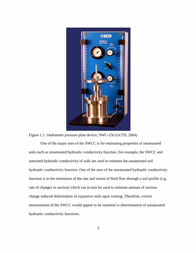
3
Figure 1.1. Oedometer pressure plate device, SWC-150 (GCTS, 2004)
One of the major uses of the SWCC is for estimating properties of unsaturated
soils such as unsaturated hydraulic conductivity function. For example, the SWCC and
saturated hydraulic conductivity of soils are used to estimate the unsaturated soil
hydraulic conductivity function. One of the uses of the unsaturated hydraulic conductivity
function is in the estimation of the rate and extent of fluid flow through a soil profile (e.g.
rate of changes in suction) which can in turn be used to estimate amount of suction-
change induced deformation of expansive soils upon wetting. Therefore, correct
measurement of the SWCC would appear to be essential to determination of unsaturated
hydraulic conductivity functions.
4
1.2. Problem Statement
Even though the soil water characteristic curve has been measured and used by
numerous researchers throughout the years, the effect of volume change of high volume
change soils (e.g. oil sands tailings, expansive soils, and collapsible soils) has rarely been
considered when determining the SWCC's that are used in estimation of soil properties.
This may lead to inaccuracies in the SWCC's, including the air-entry value. It has been
the common practice to estimate some of the major unsaturated soil property functions
(e.g., unsaturated hydraulic conductivity function, shear strength) by using the SWCC,
further demonstrating the importance of accurate determination of the SWCC.
In recent years, the importance of considering the volume change of soils during
suction change has been recognized by a number of researchers, including Salager et al.
(2010), Pe´ron et al. (2007), Nuth and Laloui (2011), Stange and Horn (2005), Mbonimpa
et al. (2006), Perez-Garcia, et al. (2008), and Fredlund and Houston, (2013). Through
literature study it was found that the effect of net normal stress which is applied to the
soil specimen during the SWCC test has also been under-studied. Only very few
researchers have conducted studies for finding the impact of net normal stress on
SWCC's (both drying and wetting cycles of SWCC) which in this research was found to
be important, particularly with regard to effect of net normal stress on volume change of
the soil during SWCC testing on expansive clays. Furthermore, the effect of initial state
of the soil specimen including initial moisture content on SWCC has not been studied by
a lot of researchers. It is known that the initial condition of the soil (slurry versus

5
compacted at or near optimum moisture content) can have a significant effect on the
SWCC of the soil, particularly with regard to soil volume change (Fredlund, 2002).
Correction of SWCC's for soil volume change during the test may have a
considerable impact on air-entry value and shape of the SWCC, depending on the amount
of volume change that occurs in response to changes in soil matric suction. This, in turn,
may have a significant impact on unsaturated soil properties derived from the SWCC's
(e.g. soil hydraulic properties such as unsaturated hydraulic conductivity function). No
studies on numerical modeling of the effect of correction of the SWCC for soil volume
change on hydraulic properties of the soils (and its impact on amount of wetting-induced
deformation of expansive soils was found in the literature, and this represents another
important area of study that is addressed in this research.
1.3. Research Objectives and Scope of Work
An extensive literature review was conducted regarding the methods of SWCC
determination and the models available to best-fit the SWCC data obtained from
laboratory experiments. This literature search SWCC's included the study of typical air-
entry values and hysteresis. Emphasis was placed upon the SWCC's of clays. Use of soil
water characteristic curves in constitutive relations for unsaturated soils such as
unsaturated hydraulic conductivity functions was also studied through a literature search.
Some of the commonly-used equations for estimating unsaturated hydraulic conductivity
functions of soils based on the SWCC were studied. This part of the literature search
included studying the methodologies used for developing the equations for estimating
6
unsaturated hydraulic conductivity functions as well as the applications of the proposed
equations.
The importance of correcting the SWCC's (including SWCC's in terms of
volumetric water content and degree of saturation) for soil volume change that occurs
during the SWCC test was studied through literature search and laboratory experiments.
Additional literature search and laboratory experiments were carried out to assess the
effect of net normal stress on the shape of SWCC with regard to the soil volume change.
Drying and wetting SWCC experiments were conducted with various net normal stresses
to find the effect of net normal stress on volume change of expansive clays during SWCC
test. Moreover, the importance of initial condition of the specimen (slurry versus
compacted specimen) was evaluated through literature search and laboratory
experiments. The entire laboratory testing in this research was performed on expansive
soils, as an example of relatively high volume-change materials of interest in
geotechnical engineering applications.
In this research, the SWCC's of three highly expansive soils were measured. The
soils tested in this study have been collected from areas in Anthem, Arizona, San
Antonio, Texas, and Denver, Colorado. For simplicity these soils will be referred to as
Anthem, San Antonio, and Colorado through this dissertation. Properties of the soils
tested as well as the test procedure and results are presented in this report. Volume
change of these soils during suction change was measured and taken into account for
establishing the SWCC's. It was found that volume change consideration plays a major
7
role in the shape of the SWCC particularly regarding the air-entry value (AEV)
determination.
In addition to the SWCC tests conducted on compacted specimens, slurry
specimens of Anthem, Colorado, and San Antonio soils were also tested and the resulting
SWCC's were compared against the SWCC's obtained from the compacted specimens of
the same soils. It was found that the initial state of the specimen has a significant effect
on the shape of the SWCC, particularly due to high volume change of slurry specimens
during the test.
As the next part of this study, complete determination of the SWCC's for three
soils of Anthem, Colorado, and San Antonio were carried out which included both drying
and wetting paths. During this set of tests, effect of net normal stress and hysteresis on
the SWCC of expansive soils was studied. The net normal stress values applied to the soil
specimens were varied form only a seating load (7 kPa) to around 54% of the swell
pressure of the soil samples. Suction measurement and control methods used in the
laboratory testing included axis translation and filter paper methods.
The last part of this study included numerical modeling of one-dimensional fluid
flow through an expansive soil profile and the deformations due to changes in suction
under constant net normal stress. In this study, the rate of changes in suction through the
soil was evaluated using three computer programs SVFLUX, VADOSE/W, and CODE-
BRIGHT. In this numerical modeling study, the effect of correcting SWCC for soil
volume change on hydraulic properties of the unsaturated soils and on results of the fluid
flow modeling (rate of advancement of wetted front and degree of saturation within the
8
profile) was assessed. Furthermore, effect of volume change correction of SWCC on
amount of deformation caused by changes in soil suction was evaluated.
1.4. Report Organization
This report is organized in the following manner. After the introduction which
covers the research objectives and scope of work, Chapter 2 presents an extensive
literature review on the methods used for measuring and generating SWCC's. Also air-
entry value of clays and hysteresis present in SWCC's that were studied through literature
search are presented. Furthermore, impact of net normal stress (i.e. stress state) and initial
state of the specimen (slurry versus compacted) on SWCC is summarized. An extensive
literature review was carried out regarding state of practice for correcting SWCC's for
soil volume change that occurs during SWCC test. Equations developed by researchers to
best-fit SWCC data was also studied and presented. Also use of the SWCC in constitutive
relations for unsaturated soils, particularly unsaturated hydraulic properties was studied.
An extensive literature review was conducted on most common models used for
unsaturated hydraulic conductivity of soils. Three of the most common models (which
are used in most of the available computer codes for modeling of fluid flow through
soils) were studied and are presented in more detail in Chapter 2 (i.e. literature review
chapter).
Chapter 3 covers the laboratory testing program that was carried out as a part of
this study. This chapter presents the test methods and procedures, laboratory equipment,
and basic properties of the soils used in the study. Results of the testing program and
necessary comparisons and analyses of the results are also illustrated in this chapter.
9
Chapter 4 includes the numerical modeling conducted of the expansive soils
tested in laboratory as a part of this study. In this chapter the computer programs and
models and equations utilized are described along with the data used regarding geometry
of the model, boundary conditions, materials properties and analysis type. This chapter
covers numerical modeling for one-dimensional fluid flow through the soil as well as
coupled flow-deformation modeling. The results of each modeling effort, as well as the
analysis and synthesis of the results, are presented in chapter 4.
Chapter 5 includes the numerical modeling conducted for oil sands tailings. Oil
sands tailings exhibit extreme volume change upon change in suction. The properties of
this material were obtained from literature. Numerical modeling was done on oil sands
tailings to establish trends for results and the models, material properties and analyses of
results for this set of numerical modeling is presented Chapter 5.
Chapter 6 summarizes the main findings, contributions, and conclusions of this
research. Chapter 6 also presents recommendations for future research work. References
and several supporting Appendices are also included at the end of this research.
10
Chapter 2
LITERATURE REVIEW
2.1. Introduction
The soil water characteristic curve (SWCC) is a measure of amount of water in
soils at different suctions. Among the different methods for applying suction to the soil
specimens as a part of SWCC tests, the axis translation method has been utilized most
widely, since in this method suction is easily controlled.
The axis-translation technique allows the pore-water pressure, uw, in an
unsaturated soil to be measured (or controlled) using a ceramic disk with very small pores
(i.e. high air-entry disk- HAED) (Powers et al., 2007). A HAED acts as a semi-
permeable membrane that separates air and water. The separation of water and air phases
can be achieved only up to the air-entry value of the disk, which is the matric suction
beyond which free air passes through the disk.
The SWCC can be used to estimate unsaturated soil property functions such as
unsaturated hydraulic conductivity. Therefore, the accuracy of the unsaturated soil
property functions depends on the accuracy of the SWCC. Several factors such as soil
structure, initial water content, void ratio, and compaction method can have significant
effects on the SWCC. Among these factors, stress history and initial water content has
been reported to have the greatest effect on the soil structure, which in turn plays a
significant role on the shape of the SWCC (Zhou et al. 2005).The air-entry value of the
soil and the rate of desaturation is reportedly affected by the initial density and amount of
disturbance to the soil (Fredlund and Houston, 2009). A distinctive point on SWCC is the
11
air-entry value. The air-entry value (AEV) corresponds to the value of matric suction at
which the largest voids within the soil specimen begin to drain freely.
The amount of water in the soil versus suction can be represented by SWCC using
three terms of gravimetric water content, volumetric water content, and degree of
saturation. The SWCC in terms of gravimetric water content can be most easily measured
in laboratory as it only include measurement of mass of water and mass of dry soil. The
degree of saturation and volumetric water content require a measurement of the volume
of the soil specimen in addition to measurement of the water content. Measurement of
volume change of unsaturated soils has been carried out by a number of researchers and
is reportedly quite demanding and requires more time and experimental care (Mbonimpa
et al. 2006).
2.2. Soil Water Characteristic Curve Determination
Figure 2.1 presented by Fredlund and Houston (2009) shows a typical SWCC.
There are four key parameters on any soil-water characteristic curve (Pham et al. 2003).
These are the water content at zero soil suction (i.e. water content of the soil at
saturation), the air-entry value, the slope of the curve (particularly between the air-entry
and residual points) and the residual water content. Three zones of desaturation can be
seen within the curve. The key features on the SWCC are the air-entry value and the
residual value for suction and water content.
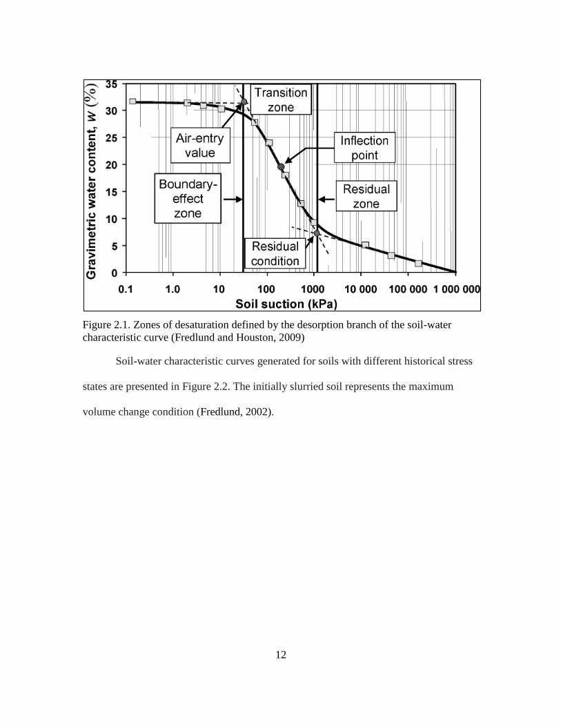
12
Figure 2.1. Zones of desaturation defined by the desorption branch of the soil-water
characteristic curve (Fredlund and Houston, 2009)
Soil-water characteristic curves generated for soils with different historical stress
states are presented in Figure 2.2. The initially slurried soil represents the maximum
volume change condition (Fredlund, 2002).
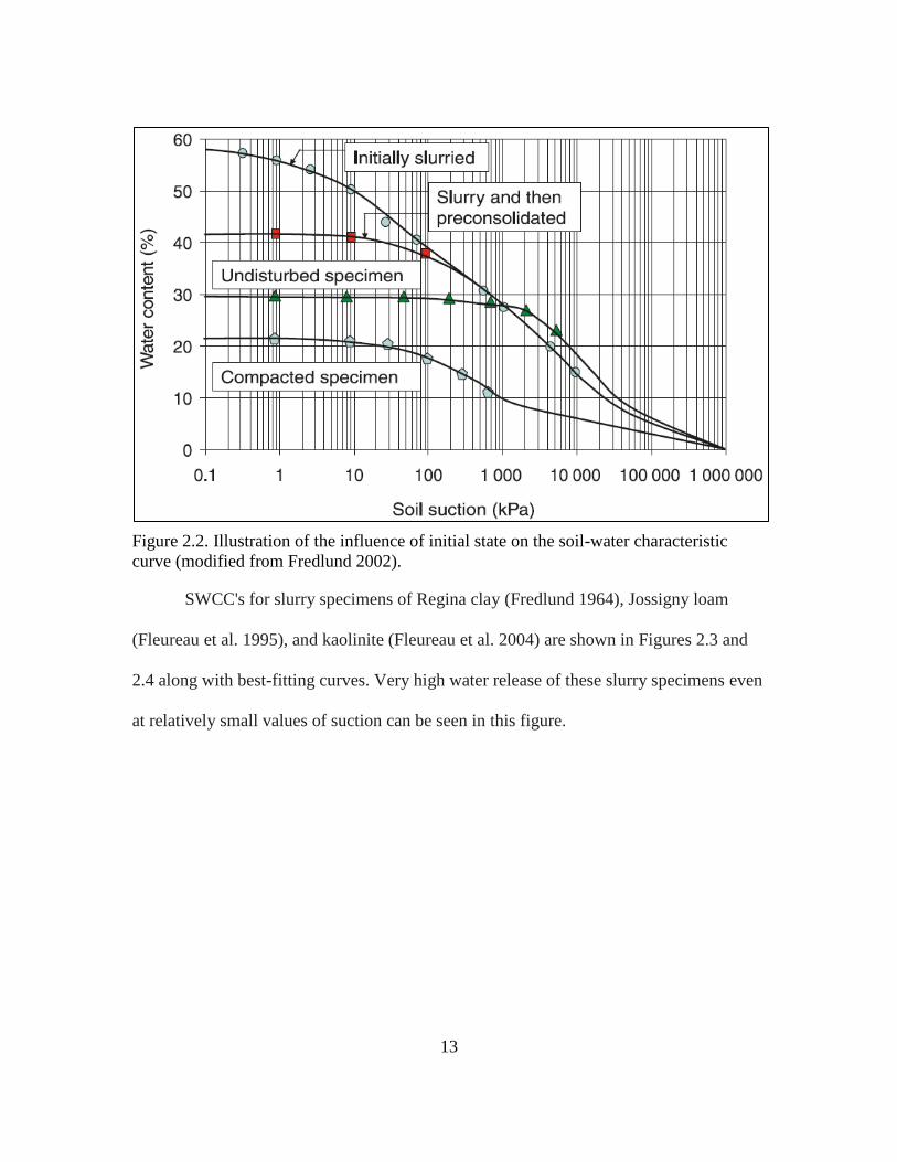
13
Figure 2.2. Illustration of the influence of initial state on the soil-water characteristic
curve (modified from Fredlund 2002).
SWCC's for slurry specimens of Regina clay (Fredlund 1964), Jossigny loam
(Fleureau et al. 1995), and kaolinite (Fleureau et al. 2004) are shown in Figures 2.3 and
2.4 along with best-fitting curves. Very high water release of these slurry specimens even
at relatively small values of suction can be seen in this figure.
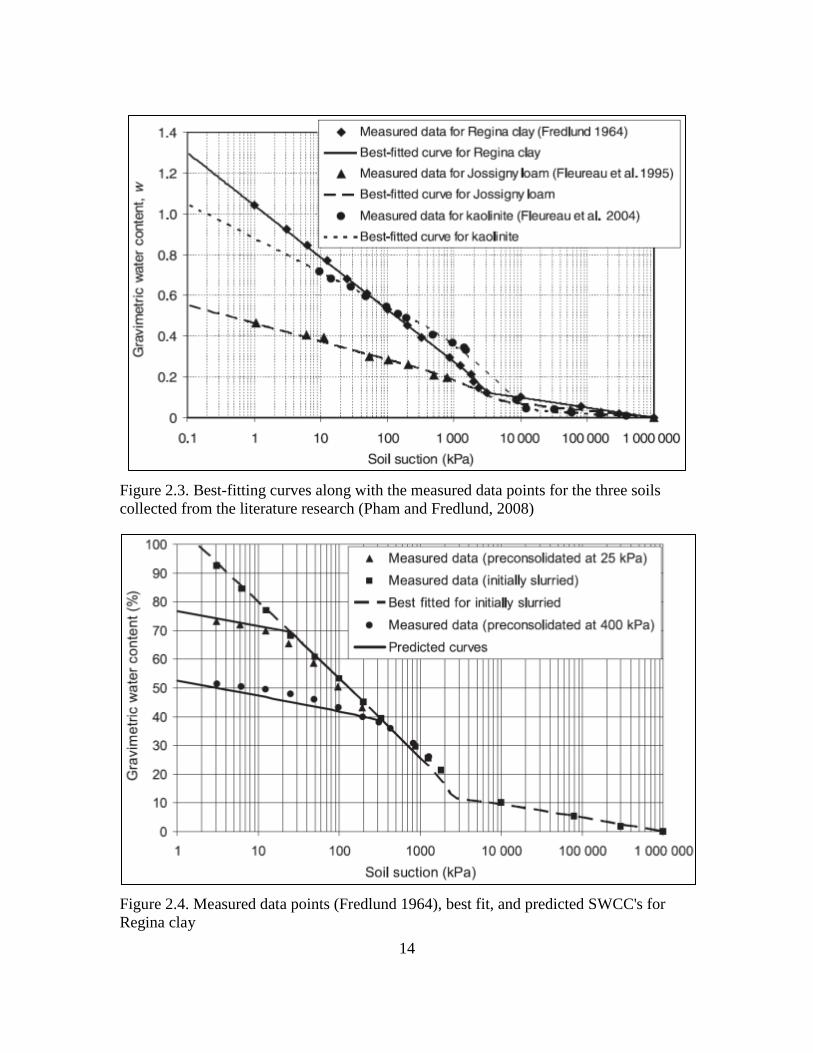
14
Figure 2.3. Best-fitting curves along with the measured data points for the three soils
collected from the literature research (Pham and Fredlund, 2008)
Figure 2.4. Measured data points (Fredlund 1964), best fit, and predicted SWCC's for
Regina clay
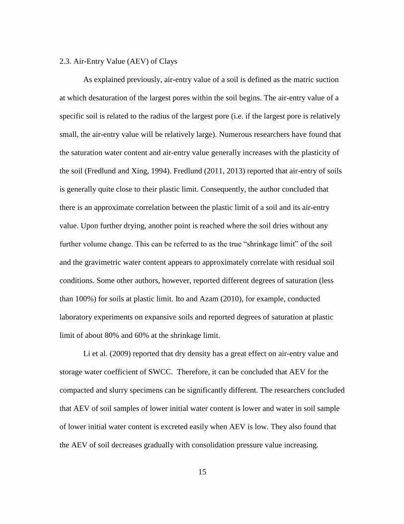
15
2.3. Air-Entry Value (AEV) of Clays
As explained previously, air-entry value of a soil is defined as the matric suction
at which desaturation of the largest pores within the soil begins. The air-entry value of a
specific soil is related to the radius of the largest pore (i.e. if the largest pore is relatively
small, the air-entry value will be relatively large). Numerous researchers have found that
the saturation water content and air-entry value generally increases with the plasticity of
the soil (Fredlund and Xing, 1994). Fredlund (2011, 2013) reported that air-entry of soils
is generally quite close to their plastic limit. Consequently, the author concluded that
there is an approximate correlation between the plastic limit of a soil and its air-entry
value. Upon further drying, another point is reached where the soil dries without any
further volume change. This can be referred to as the true “shrinkage limit” of the soil
and the gravimetric water content appears to approximately correlate with residual soil
conditions. Some other authors, however, reported different degrees of saturation (less
than 100%) for soils at plastic limit. Ito and Azam (2010), for example, conducted
laboratory experiments on expansive soils and reported degrees of saturation at plastic
limit of about 80% and 60% at the shrinkage limit.
Li et al. (2009) reported that dry density has a great effect on air-entry value and
storage water coefficient of SWCC. Therefore, it can be concluded that AEV for the
compacted and slurry specimens can be significantly different. The researchers concluded
that AEV of soil samples of lower initial water content is lower and water in soil sample
of lower initial water content is excreted easily when AEV is low. They also found that
the AEV of soil decreases gradually with consolidation pressure value increasing.
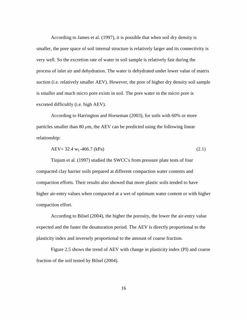
16
According to James et al. (1997), it is possible that when soil dry density is
smaller, the pore space of soil internal structure is relatively larger and its connectivity is
very well. So the excretion rate of water in soil sample is relatively fast during the
process of inlet air and dehydration. The water is dehydrated under lower value of matrix
suction (i.e. relatively smaller AEV). However, the pore of higher dry density soil sample
is smaller and much micro pore exists in soil. The pore water in the micro pore is
excreted difficultly (i.e. high AEV).
According to Harrington and Horseman (2003), for soils with 60% or more
particles smaller than 80 μm, the AEV can be predicted using the following linear
relationship:
AEV= 32.4 wL-466.7 (kPa) (2.1)
Tinjum et al. (1997) studied the SWCC's from pressure plate tests of four
compacted clay barrier soils prepared at different compaction water contents and
compaction efforts. Their results also showed that more plastic soils tended to have
higher air-entry values when compacted at a wet of optimum water content or with higher
compaction effort.
According to Bilsel (2004), the higher the porosity, the lower the air-entry value
expected and the faster the desaturation period. The AEV is directly proportional to the
plasticity index and inversely proportional to the amount of coarse fraction.
Figure 2.5 shows the trend of AEV with change in plasticity index (PI) and coarse
fraction of the soil tested by Bilsel (2004).
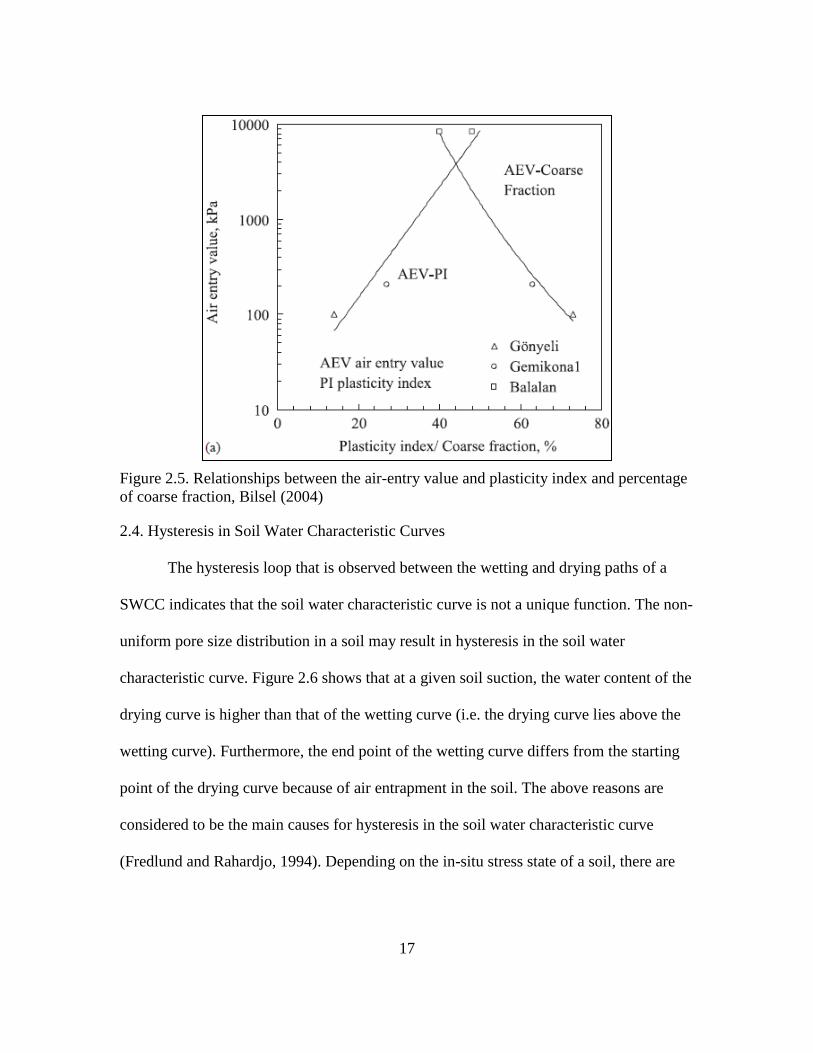
17
Figure 2.5. Relationships between the air-entry value and plasticity index and percentage
of coarse fraction, Bilsel (2004)
2.4. Hysteresis in Soil Water Characteristic Curves
The hysteresis loop that is observed between the wetting and drying paths of a
SWCC indicates that the soil water characteristic curve is not a unique function. The non-
uniform pore size distribution in a soil may result in hysteresis in the soil water
characteristic curve. Figure 2.6 shows that at a given soil suction, the water content of the
drying curve is higher than that of the wetting curve (i.e. the drying curve lies above the
wetting curve). Furthermore, the end point of the wetting curve differs from the starting
point of the drying curve because of air entrapment in the soil. The above reasons are
considered to be the main causes for hysteresis in the soil water characteristic curve
(Fredlund and Rahardjo, 1994). Depending on the in-situ stress state of a soil, there are
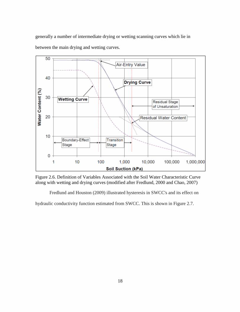
18
generally a number of intermediate drying or wetting scanning curves which lie in
between the main drying and wetting curves.
Figure 2.6. Definition of Variables Associated with the Soil Water Characteristic Curve
along with wetting and drying curves (modified after Fredlund, 2000 and Chao, 2007)
Fredlund and Houston (2009) illustrated hysteresis in SWCC's and its effect on
hydraulic conductivity function estimated from SWCC. This is shown in Figure 2.7.
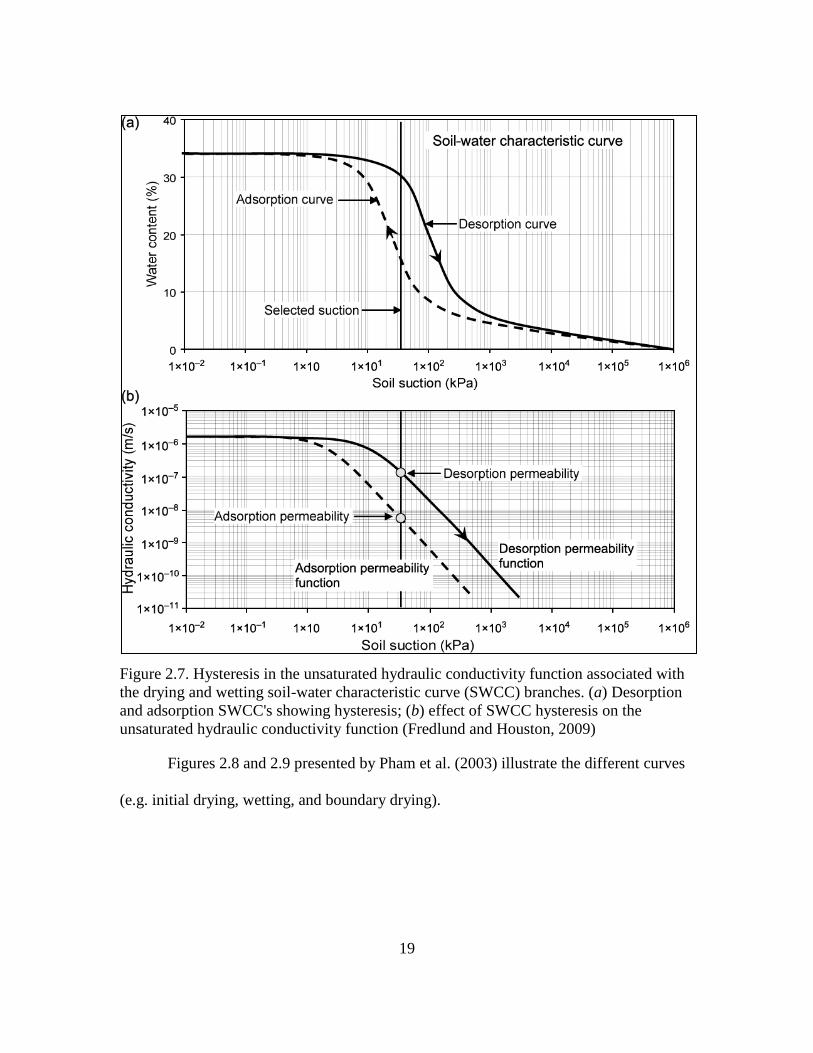
19
Figure 2.7. Hysteresis in the unsaturated hydraulic conductivity function associated with
the drying and wetting soil-water characteristic curve (SWCC) branches. (a) Desorption
and adsorption SWCC's showing hysteresis; (b) effect of SWCC hysteresis on the
unsaturated hydraulic conductivity function (Fredlund and Houston, 2009)
Figures 2.8 and 2.9 presented by Pham et al. (2003) illustrate the different curves
(e.g. initial drying, wetting, and boundary drying).
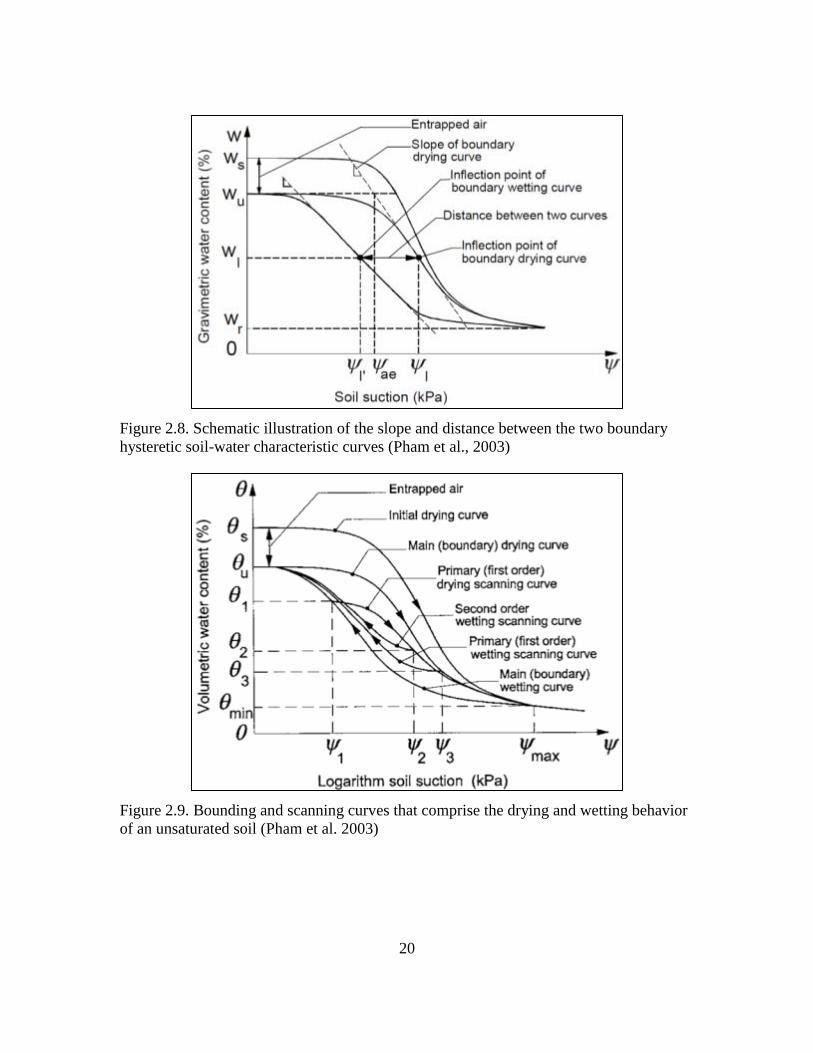
20
Figure 2.8. Schematic illustration of the slope and distance between the two boundary
hysteretic soil-water characteristic curves (Pham et al., 2003)
Figure 2.9. Bounding and scanning curves that comprise the drying and wetting behavior
of an unsaturated soil (Pham et al. 2003)
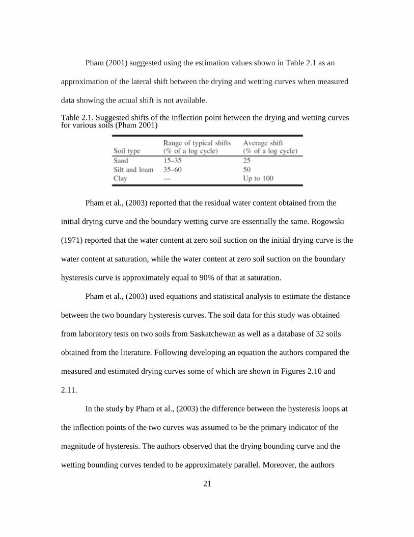
21
Pham (2001) suggested using the estimation values shown in Table 2.1 as an
approximation of the lateral shift between the drying and wetting curves when measured
data showing the actual shift is not available.
Table 2.1. Suggested shifts of the inflection point between the drying and wetting curves for various soils (Pham 2001)
Pham et al., (2003) reported that the residual water content obtained from the
initial drying curve and the boundary wetting curve are essentially the same. Rogowski
(1971) reported that the water content at zero soil suction on the initial drying curve is the
water content at saturation, while the water content at zero soil suction on the boundary
hysteresis curve is approximately equal to 90% of that at saturation.
Pham et al., (2003) used equations and statistical analysis to estimate the distance
between the two boundary hysteresis curves. The soil data for this study was obtained
from laboratory tests on two soils from Saskatchewan as well as a database of 32 soils
obtained from the literature. Following developing an equation the authors compared the
measured and estimated drying curves some of which are shown in Figures 2.10 and
2.11.
In the study by Pham et al., (2003) the difference between the hysteresis loops at
the inflection points of the two curves was assumed to be the primary indicator of the
magnitude of hysteresis. The authors observed that the drying bounding curve and the
wetting bounding curves tended to be approximately parallel. Moreover, the authors
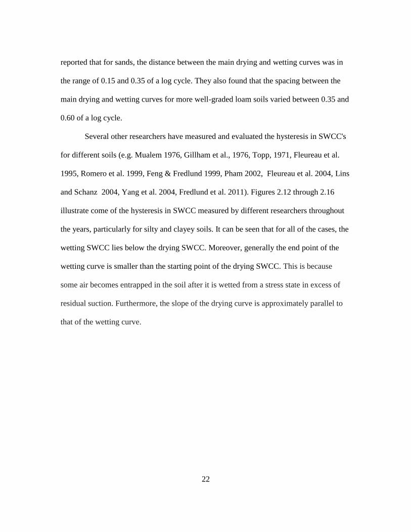
22
reported that for sands, the distance between the main drying and wetting curves was in
the range of 0.15 and 0.35 of a log cycle. They also found that the spacing between the
main drying and wetting curves for more well-graded loam soils varied between 0.35 and
0.60 of a log cycle.
Several other researchers have measured and evaluated the hysteresis in SWCC's
for different soils (e.g. Mualem 1976, Gillham et al., 1976, Topp, 1971, Fleureau et al.
1995, Romero et al. 1999, Feng & Fredlund 1999, Pham 2002, Fleureau et al. 2004, Lins
and Schanz 2004, Yang et al. 2004, Fredlund et al. 2011). Figures 2.12 through 2.16
illustrate come of the hysteresis in SWCC measured by different researchers throughout
the years, particularly for silty and clayey soils. It can be seen that for all of the cases, the
wetting SWCC lies below the drying SWCC. Moreover, generally the end point of the
wetting curve is smaller than the starting point of the drying SWCC. This is because
some air becomes entrapped in the soil after it is wetted from a stress state in excess of
residual suction. Furthermore, the slope of the drying curve is approximately parallel to
that of the wetting curve.
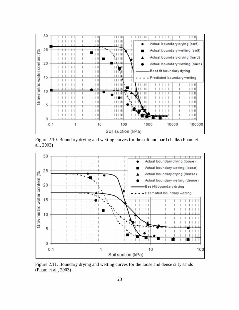
23
Figure 2.10. Boundary drying and wetting curves for the soft and hard chalks (Pham et
al., 2003)
Figure 2.11. Boundary drying and wetting curves for the loose and dense silty sands
(Pham et al., 2003)
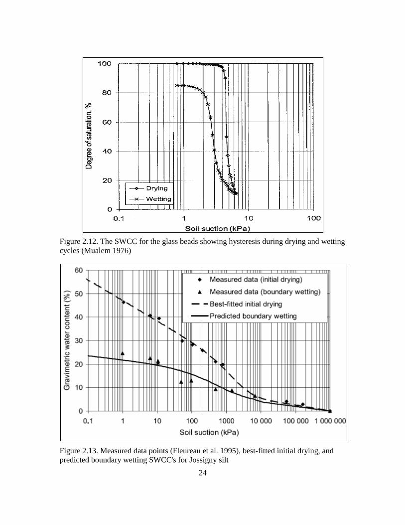
24
Figure 2.12. The SWCC for the glass beads showing hysteresis during drying and wetting
cycles (Mualem 1976)
Figure 2.13. Measured data points (Fleureau et al. 1995), best-fitted initial drying, and
predicted boundary wetting SWCC's for Jossigny silt
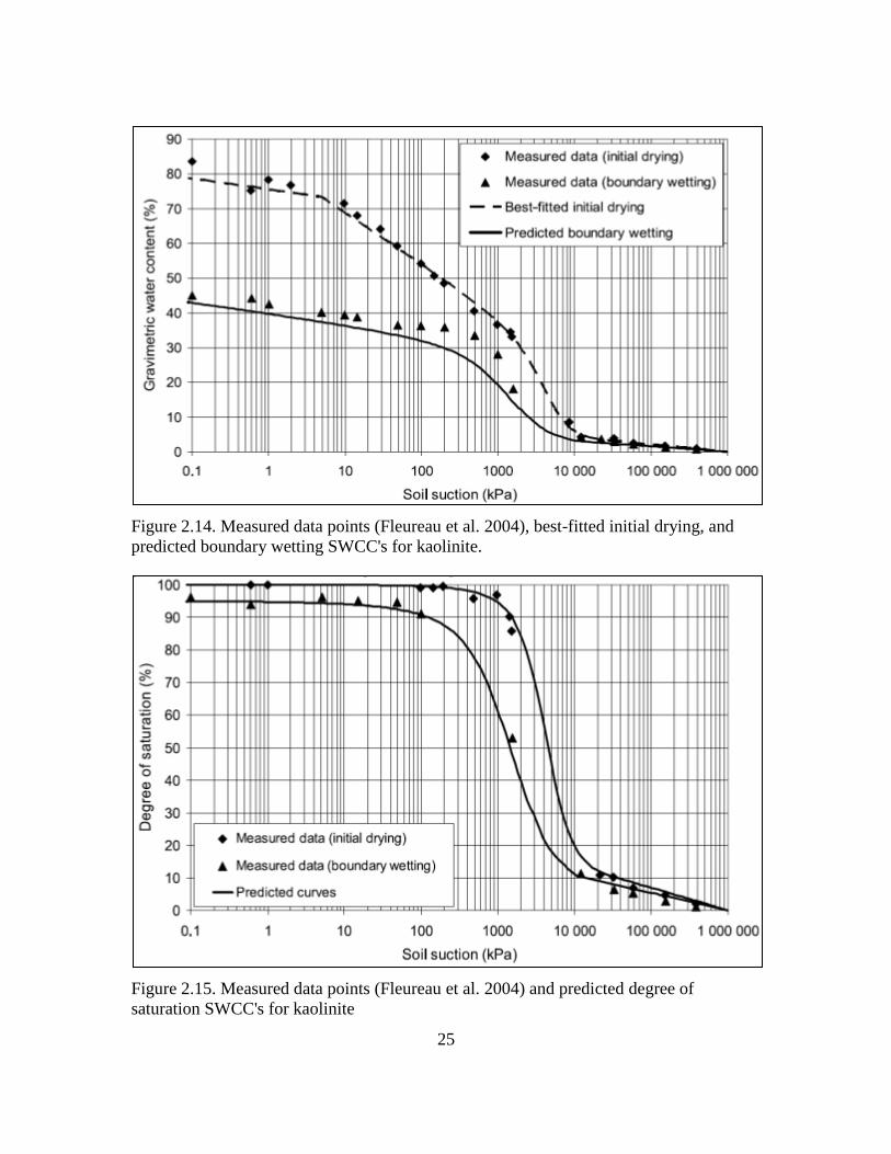
25
Figure 2.14. Measured data points (Fleureau et al. 2004), best-fitted initial drying, and
predicted boundary wetting SWCC's for kaolinite.
Figure 2.15. Measured data points (Fleureau et al. 2004) and predicted degree of
saturation SWCC's for kaolinite
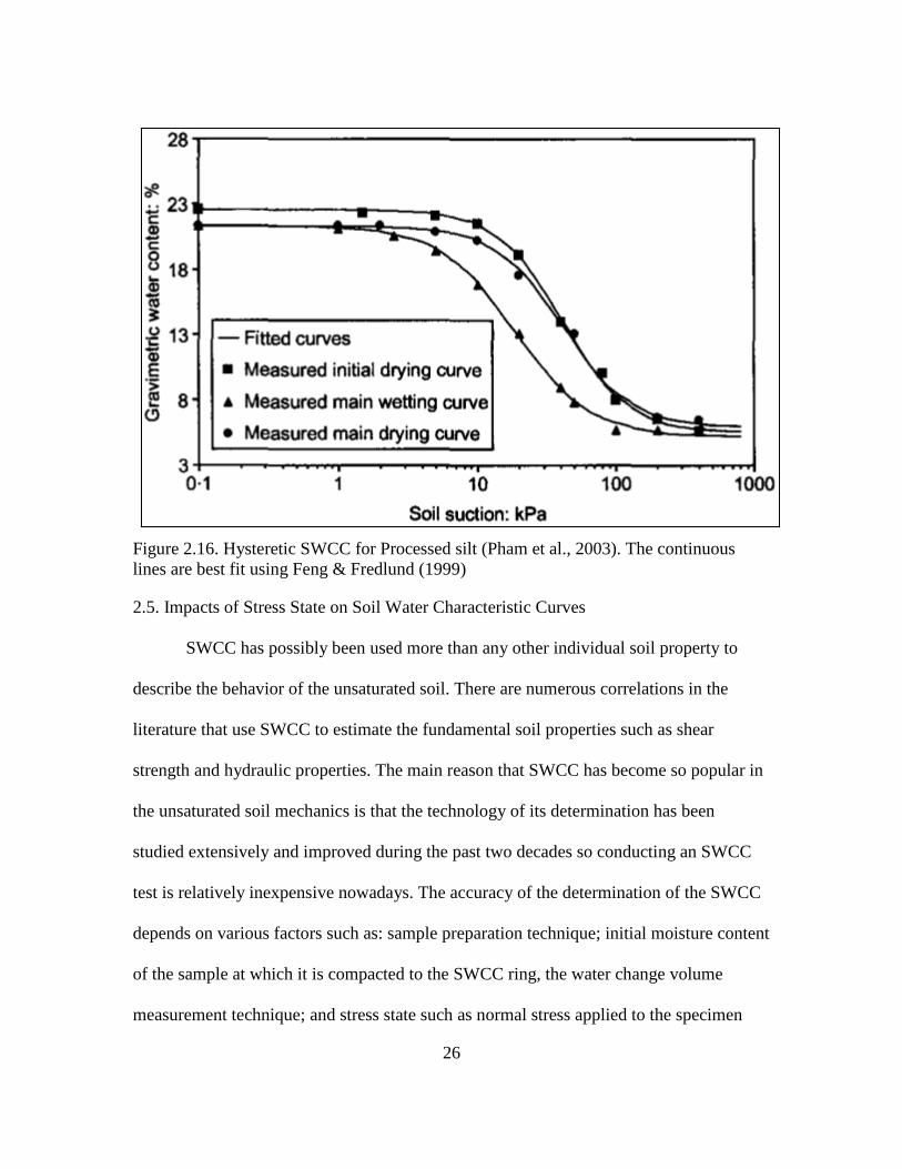
26
Figure 2.16. Hysteretic SWCC for Processed silt (Pham et al., 2003). The continuous
lines are best fit using Feng & Fredlund (1999)
2.5. Impacts of Stress State on Soil Water Characteristic Curves
SWCC has possibly been used more than any other individual soil property to
describe the behavior of the unsaturated soil. There are numerous correlations in the
literature that use SWCC to estimate the fundamental soil properties such as shear
strength and hydraulic properties. The main reason that SWCC has become so popular in
the unsaturated soil mechanics is that the technology of its determination has been
studied extensively and improved during the past two decades so conducting an SWCC
test is relatively inexpensive nowadays. The accuracy of the determination of the SWCC
depends on various factors such as: sample preparation technique; initial moisture content
of the sample at which it is compacted to the SWCC ring, the water change volume
measurement technique; and stress state such as normal stress applied to the specimen
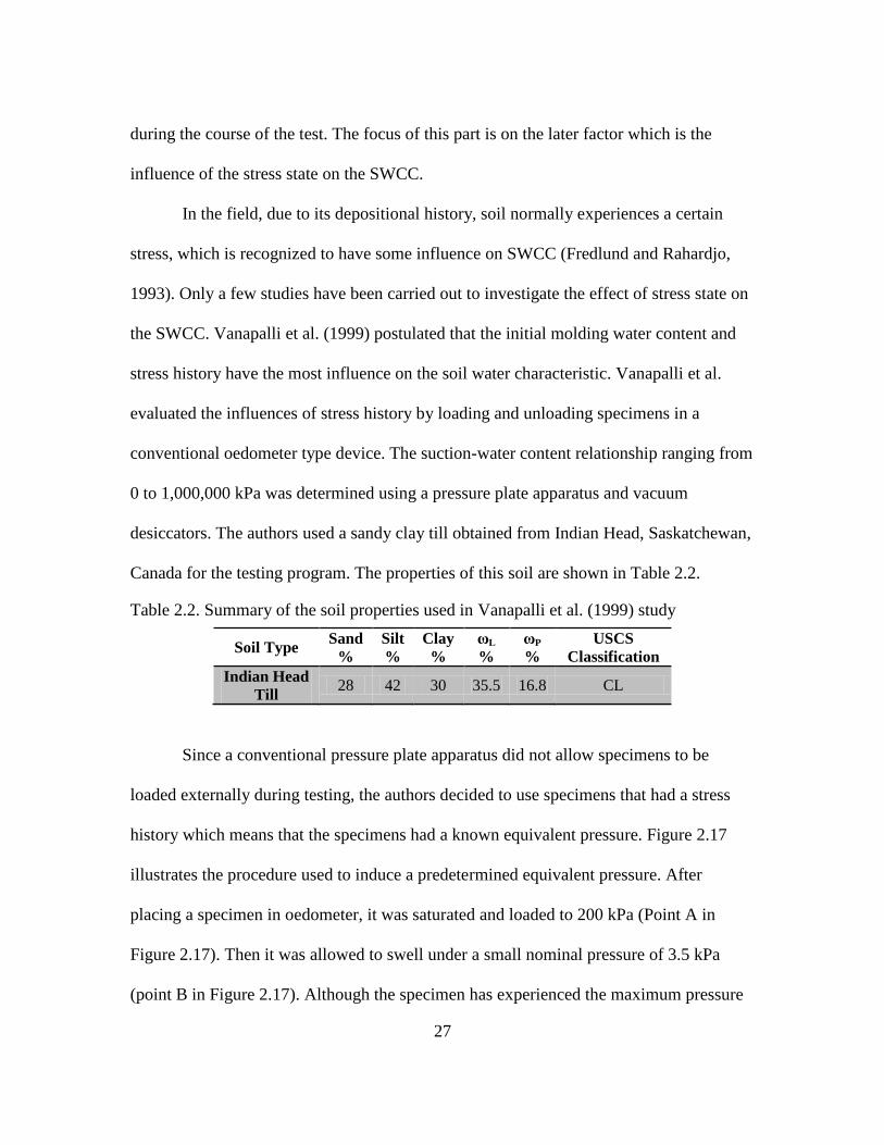
27
during the course of the test. The focus of this part is on the later factor which is the
influence of the stress state on the SWCC.
In the field, due to its depositional history, soil normally experiences a certain
stress, which is recognized to have some influence on SWCC (Fredlund and Rahardjo,
1993). Only a few studies have been carried out to investigate the effect of stress state on
the SWCC. Vanapalli et al. (1999) postulated that the initial molding water content and
stress history have the most influence on the soil water characteristic. Vanapalli et al.
evaluated the influences of stress history by loading and unloading specimens in a
conventional oedometer type device. The suction-water content relationship ranging from
0 to 1,000,000 kPa was determined using a pressure plate apparatus and vacuum
desiccators. The authors used a sandy clay till obtained from Indian Head, Saskatchewan,
Canada for the testing program. The properties of this soil are shown in Table 2.2.
Table 2.2. Summary of the soil properties used in Vanapalli et al. (1999) study
Soil Type Sand
%
Silt
%
Clay
%
ωL
%
ωP
%
USCS
Classification
Indian Head
Till 28 42 30 35.5 16.8 CL
Since a conventional pressure plate apparatus did not allow specimens to be
loaded externally during testing, the authors decided to use specimens that had a stress
history which means that the specimens had a known equivalent pressure. Figure 2.17
illustrates the procedure used to induce a predetermined equivalent pressure. After
placing a specimen in oedometer, it was saturated and loaded to 200 kPa (Point A in
Figure 2.17). Then it was allowed to swell under a small nominal pressure of 3.5 kPa
(point B in Figure 2.17). Although the specimen has experienced the maximum pressure
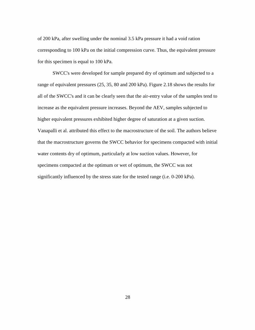
28
of 200 kPa, after swelling under the nominal 3.5 kPa pressure it had a void ration
corresponding to 100 kPa on the initial compression curve. Thus, the equivalent pressure
for this specimen is equal to 100 kPa.
SWCC's were developed for sample prepared dry of optimum and subjected to a
range of equivalent pressures (25, 35, 80 and 200 kPa). Figure 2.18 shows the results for
all of the SWCC's and it can be clearly seen that the air-entry value of the samples tend to
increase as the equivalent pressure increases. Beyond the AEV, samples subjected to
higher equivalent pressures exhibited higher degree of saturation at a given suction.
Vanapalli et al. attributed this effect to the macrostructure of the soil. The authors believe
that the macrostructure governs the SWCC behavior for specimens compacted with initial
water contents dry of optimum, particularly at low suction values. However, for
specimens compacted at the optimum or wet of optimum, the SWCC was not
significantly influenced by the stress state for the tested range (i.e. 0-200 kPa).
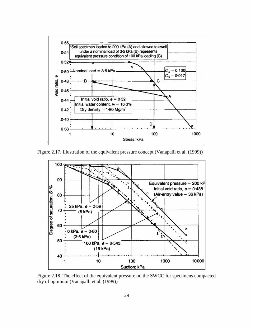
29
`
Figure 2.17. Illustration of the equivalent pressure concept (Vanapalli et al. (1999))
Figure 2.18. The effect of the equivalent pressure on the SWCC for specimens compacted
dry of optimum (Vanapalli et al. (1999))
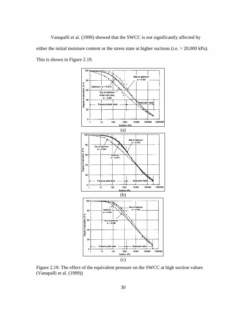
30
Vanapalli et al. (1999) showed that the SWCC is not significantly affected by
either the initial moisture content or the stress state at higher suctions (i.e. > 20,000 kPa).
This is shown in Figure 2.19.
(a)
(b)
(c)
Figure 2.19. The effect of the equivalent pressure on the SWCC at high suction values
(Vanapalli et al. (1999))
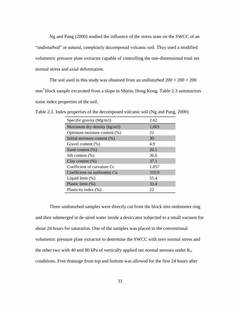
31
Ng and Pang (2000) studied the influence of the stress state on the SWCC of an
“undisturbed” or natural, completely decomposed volcanic soil. They used a modified
volumetric pressure plate extractor capable of controlling the one-dimensional total net
normal stress and axial deformation.
The soil used in this study was obtained from an undisturbed 200 × 200 × 200
mm3
block sample excavated from a slope in Shatin, Hong Kong. Table 2.3 summarizes
some index properties of the soil.
Table 2.3. Index properties of the decomposed volcanic soil (Ng and Pang, 2000)
Specific gravity (Mg/m3) 2.62
Maximum dry density (kg/m3) 1,603
Optimum moisture content (%) 22
Initial moisture content (%) 30
Gravel content (%) 4.9
Sand content (%) 20.1
Silt content (%) 36.6
Clay content (%) 37.1
Coefficient of curvature Cc 1.057
Coefficient on uniformity Cu 319.9
Liquid limit (%) 55.4
Plastic limit (%) 33.4
Plasticity index (%) 22
Three undisturbed samples were directly cut from the block into oedometer ring
and then submerged in de-aired water inside a desiccator subjected to a small vacuum for
about 24 hours for saturation. One of the samples was placed in the conventional
volumetric pressure plate extractor to determine the SWCC with zero normal stress and
the other two with 40 and 80 kPa of vertically applied net normal stresses under Ko
conditions. Free drainage from top and bottom was allowed for the first 24 hours after
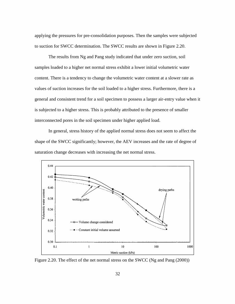
32
applying the pressures for pre-consolidation purposes. Then the samples were subjected
to suction for SWCC determination. The SWCC results are shown in Figure 2.20.
The results from Ng and Pang study indicated that under zero suction, soil
samples loaded to a higher net normal stress exhibit a lower initial volumetric water
content. There is a tendency to change the volumetric water content at a slower rate as
values of suction increases for the soil loaded to a higher stress. Furthermore, there is a
general and consistent trend for a soil specimen to possess a larger air-entry value when it
is subjected to a higher stress. This is probably attributed to the presence of smaller
interconnected pores in the soil specimen under higher applied load.
In general, stress history of the applied normal stress does not seem to affect the
shape of the SWCC significantly; however, the AEV increases and the rate of degree of
saturation change decreases with increasing the net normal stress.
Figure 2.20. The effect of the net normal stress on the SWCC (Ng and Pang (2000))
33
2.6. Correcting Soil Water Characteristic Curves for Soil Volume Change
Suction induced volume change in expansive soils occurs due to changes in the
water content of the soil which affects the stress equilibrium of the soil. Consequently,
when determining the SWCC of an expansive soil, it is important to consider the volume
change that occurs as the suction (and hence the water content of the soil) changes during
the test (Chao et al., 2008). This reportedly is not the common practice and the SWCC is
usually measured assuming no volume change of the soil specimen. This assumption may
not be correct for expansive soils. When determining the SWCC of an expansive soil, it is
important to consider the volume change that occurs as the suction changes during the
test (Chao et al. 2008).
Soil water characteristic curve fitting equations have been generated by a number
of researchers (e.g., Gardner 1956; Brooks and Corey 1964; van Genuchten 1980;
Fredlund and Xing 1994). Although not always mentioned, the underlying assumption of
most SWCC fitting equations is that the soil is sufficiently stiff so that there is no change
in void ratio of the soil (i.e. soil volume change) during the test (Mbonimpa et al., 2006,
Chiu and Ng, 2012). Nonetheless, some of these equations have been extended for use in
case of high volume change materials. Pham and Fredlund (2008) proposed two SWCC
equations for best-fitting the SWCC for a wide range of soils types including high
volume change clays. A number of researchers have attempted to predict the SWCC's of
expansive soils (Chertkov 2004; Mbonimpa et al. 2006). Gallipoli et al. (2002, 2003)
have proposed an expression for the degree of saturation based on the well-known van
Genuchten (1980) model, where the shape parameter which is related to the air-entry
34
value, is expressed as a function of void ratio. The van Genuchten (1980) model has also
been used by Stange and Horn (2005) who proposed an expression for volumetric water
content by accounting for the dependence of the saturated and residual volumetric water
contents and the shape parameters on void ratio e.
Mbonimpa et al. (2006) extended modified Kovács model which predicts the soil
water characteristic curve using basic properties for incompressible soils to clayey soils
showing suction induced volume change. The authors performed this by introducing the
shrinkage curve in the formulation. The authors used previously measured data points for
soil water characteristic curve and shrinkage curve from SOILVISION (SoilVision
Systems Ltd., 1999), Fleureau et al. (1993, 2002), and Biarez et al. (1987) for validating
their model.
A soil volume measurement method that has been used by some researchers is
measuring the displaced volume of a fluid when the soil sample is dipped in it. Salager et
al. (2010) recommended the use of Kerdane as this fluid was found to generate
reasonable results. The principle of the method was first described by Head (1980), and
the use of Kerdane has been described among others by Zerhouni (1991) and Abou-Bekr
et al. (2005). In this method of volume measurement, the specimen gets destroyed. The
authors mentioned that due to destructiveness of this technique, it is not appropriate for
testing natural soils, where variability among specimens may become a major issue.
According to Salager et al. (2010), the water characteristic behavior of a soil is
better represented by a surface instead of the usual curve. The researchers determined the
surface based on measurement of void ratio, suction, and water content along the drying
35
path. Salager et al. (2010) established an experimental program in which suction was
applied to the previously saturated samples in a pressure-plate apparatus. At equilibrium,
the water content and void ratio of the samples were measured. The method used by the
authors for volume measurement was based on the general method using fluid
displacement described, for instance. The fluid used for volume change measurement was
Kerdane. Kerdane is light hydro-treated petroleum distillate with density of about 800
kg/m3 essentially designed for heating and used as fuel in mobile heating devices such as
domestic oil stoves.
Ng and Pang (2000) reported the issues related to volume change when
determining the SWCC of a sandy silt and clay mixture using a modified pressure plate
extractor. The authors proposed to verify the no volume change assumption throughout
the drying-wetting processes. They concluded that the conventional assumption of no
volume change in the pressure plate tests would lead to inaccurate estimation of the soil
properties.
Stange and Horn (2005) conducted laboratory experiments on sandy and silty soil
samples collected at three sites in Germany in order to determine the SWCC. They
measured the gravimetric water contents and the volumes of the samples after each
equilibration, which were used to calculate volumetric water contents. The actual soil
volume was determined using vernier caliper measurements. The authors found the
importance of considering the volume change during the tests.
Chao et al. (2008) conducted experiments on Claystone samples of the Denver
and Pierre Shale Formations obtained near Denver, Colorado using the SWC-150 device

36
and the filter paper method. The authors studied the effect of the volume changes on the
SWCC of expansive soils. The authors used calipers to measure the height and diameter
of the sample in order to determine the volume. Measurements of the weight and volume
of the sample at equilibrium were recorded throughout the experiment. The authors
reported importance of measuring the volume change during the test and correcting the
SWCC for the volume change.
Pham and Fredlund (2008) developed two equations for SWCC based on the
laboratory tests starting from a slurry condition and continuing to completely dry
conditions, during which the sample exhibited high volume changes. Both of the
proposed SWCC equations define the soil suction versus gravimetric water content over
the entire range of possible soil suctions.
Fredlund and Houston (2013) reported that not correcting SWCC's for soil
volume change that occurs during the SWCC test (particularly soils with high volume
change potential), can lead to unrealistic results namely the estimated air-entry value of
the soils. The authors described the procedure with which the SWCC obtained from
laboratory results can be corrected for volume change with the use of a shrinkage curve.
The authors suggested two approaches for correcting SWCC's for the volume change, the
first one being to use laboratory devices capable of volume change measurement. The
next method is to generate shrinkage curves which define the relationship between
gravimetric water content and void ratio of the soil tested. For developing the shrinkage
curve the authors suggested using digital micrometers for soil volume measurement.
Fredlund and Houston (2013) demonstrated the importance of considering the soil

37
volume change (as soil suction changes) by developing SWCC's for oil sands tailings and
Regina clay with and without volume change consideration and compared the results (i.e.
with particular focus on air-entry value of the soils).
These SWCC's are shown in Figures 2.21 and 2.22. The authors recommended
using volume corrected SWCC in terms of degree of saturation for the estimation of the
true air-entry value of the soil.
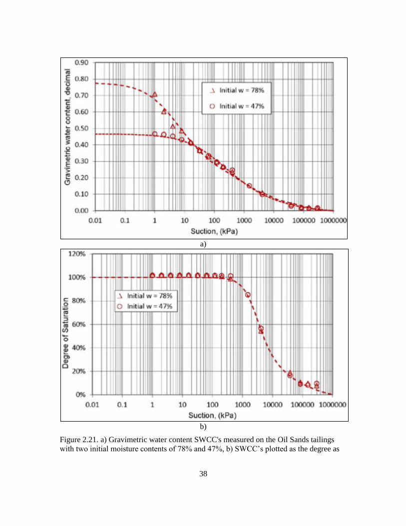
38
a)
b)
Figure 2.21. a) Gravimetric water content SWCC's measured on the Oil Sands tailings
with two initial moisture contents of 78% and 47%, b) SWCC’s plotted as the degree as
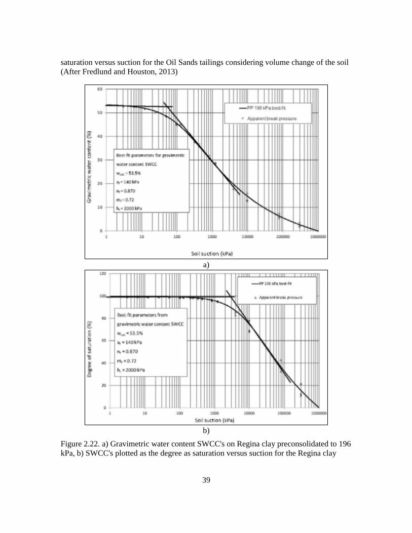
39
saturation versus suction for the Oil Sands tailings considering volume change of the soil
(After Fredlund and Houston, 2013)
a)
b)
Figure 2.22. a) Gravimetric water content SWCC's on Regina clay preconsolidated to 196
kPa, b) SWCC's plotted as the degree as saturation versus suction for the Regina clay

40
preconsolidated to 196 kPa considering volume change of the soil (After Fredlund and
Houston, 2013)
Ng and Pang (2000) studied the effect of volume changes on the SWCC during a
wetting and drying cycle using a modified volumetric pressure plate extractor in which
the total normal stress can be controlled one-dimensionally and the axial deformation can
be measured. The authors, like many others, recognized the importance of volume change
measurement and consideration in generating SWCC's.
Chiu and Ng (2012) conducted a laboratory study in which they used a modified
triaxial apparatus and a one-dimensional stress controllable pressure plate apparatus to
measure the SWCC. The modified apparatus used in their study is a double-cell triaxial
system where an open-ended, bottle-shaped inner cell is installed inside a conventional
triaxial cell together with a differential pressure transducer to measure the total volume
change of a specimen (schematic shown in Figure 2.23). The authors used the volume
measurements throughout the test for generating volume corrected SWCC in terms of
degree of saturation. Throughout the drying and wetting tests, the vertical displacement,
volume change, and water volume change of the specimens were continuously
monitored. The authors found it important to account for volume change when
determining SWCC. The authors recommended use of degree of saturation SWCC.
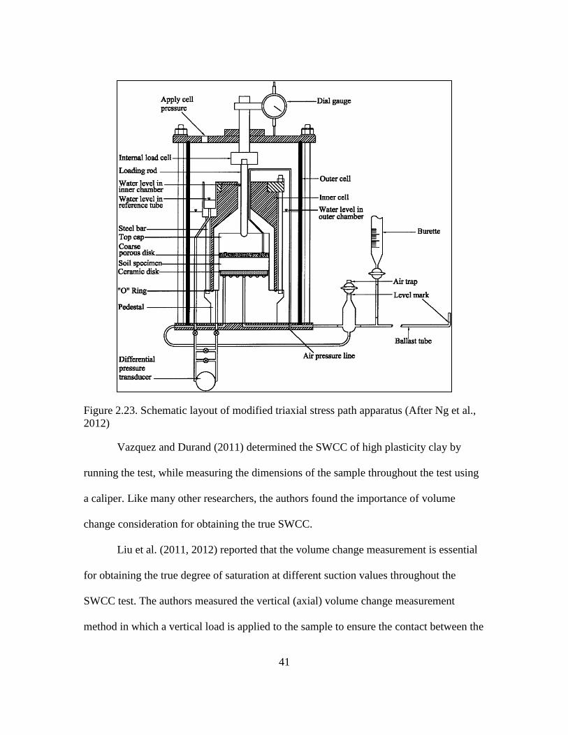
41
Figure 2.23. Schematic layout of modified triaxial stress path apparatus (After Ng et al.,
2012)
Vazquez and Durand (2011) determined the SWCC of high plasticity clay by
running the test, while measuring the dimensions of the sample throughout the test using
a caliper. Like many other researchers, the authors found the importance of volume
change consideration for obtaining the true SWCC.
Liu et al. (2011, 2012) reported that the volume change measurement is essential
for obtaining the true degree of saturation at different suction values throughout the
SWCC test. The authors measured the vertical (axial) volume change measurement
method in which a vertical load is applied to the sample to ensure the contact between the
42
sample and the confining ring. This method, obviously assumes that the full contact of
soil and ring is maintained throughout the test, therefore, considerable volume
measurement errors may occur for the cases in which the full contact of soil and
confining ring is not maintained throughout the test. The authors developed a modified
SWCC device which can measure and record volume changes during the test. Liu et al.
(2011, 2012) also evaluated the effect of volume change on the SWCC. They found the
volume change of the soil to be an important factor in the soil SWCC. The authors
reported the case in which the initial volumetric water content of the soil was 0.1. For this
case, a volume change of 3% occurred during the test, and not considering it led to 0.3%
error in the volumetric water content determination. The authors reported that the errors
become larger with larger initial water content values of the soil.
Cui et al. (2006) conducted SWCC tests and developed curves for Romainville
clay from the basin of Paris. Two suction control methods were used: 1) the osmotic
method for low suction range (1-6.1 MPa) and 2) the vapor equilibrium technique for
high suction range (6.1- 216 MPa). The authors followed both wetting and drying curves
and at each suction soil samples were weighed and the volume of samples was
determined by using a mercury immersion system. For the volume measurement of the
soil, the soil samples were first weighed in air, then immersed in mercury and weighed
again. The obtained weights allowed the volume to be determined.
Qi and Michel (2011) developed an apparatus for continues measurement of the
SWCC and shrink/swell properties of soil during wetting/drying cycles. During the test
with this apparatus, sample height, weight and pressure head were recorded every minute

43
during drying and wetting cycles using a linear variable differential transducer (LVDT), a
balance, and a ceramic cup inserted at the center of the sample and connected to a
pressure transmitter.
Huang et al. (1998) proposed a model to fit SWCC data for highly compressible
materials. However, their model did not allow representation of some features that are
relevant for highly compressible materials, such as nonlinear variation of the void ratio
for suctions lower than the air-entry value, partial desaturation that occurs in the vicinity
of the air-entry value, and variation of the void ratio for suctions higher than the air-entry
value (Parent et al., 2007).
Price and Schlotzhauer (1999) reported that accounting for suction induced
volumetric changes plays a significant role in the accuracy of the SWCC. Cabral et al.
(2004) described a testing apparatus, based on the axis translation technique that allows
measurement of volumetric changes continuously during determination of the SWCC in
highly compressible materials.
Parent et al. (2007) conducted a test in which water content, matric suction, and
volumetric deformation data of the material tested were obtained using an experimental
technique that allowed determination of the SWCC's of highly compressible materials
(such as highly plastic clays). Additionally, Parent et al. (2007) reported that volumetric
changes occurred during desaturation (i.e. shrinkage) can significantly influence the
shape of the SWCC. The authors mentioned that specifically, the volumetric changes
affect the calculated volumetric water content or degree of saturation. They found that
volumetric water contents are underestimated if volume changes are not accounted for,

44
which leads to inaccuracies in the SWCC's, thus inaccurately predicted unsaturated
hydraulic conductivity functions that are based on SWCC's. The authors also developed a
new model for describing the suction induced consolidation curve (void ratio function)
and SWCC for soils with high volume change potential. The authors recommended that
in the case of soils with high volume change potential, the air-entry value should be
determined on a degree of saturation versus suction relationship, rather than on the
volumetric water content versus suction curve, because the volumetric water content of a
compressible specimen can start to decrease while the material remains saturated, which
might be misleading when trying to determine air-entry value on such a curve.
Nuth and Laloui (2008) recommended using degree of saturation SWCC as
opposed to gravimetric moisture content. The authors reported that when the soil
undergoes volume change during a suction increase, only the degree of saturation
variable clearly defines the air-entry value for the soil (as opposed to gravimetric and
volumetric water content).
Parent et al. (2007) presented a set of plots comparing the SWCC's with and
without volume change consideration. Based on the data, the authors found that
volumetric water contents are underestimated if volume changes are not considered,
particularly at high matric suction values. They concluded that the degree of saturation is
significantly higher when accounting for volume changes.
Li et al. (2007) obtained the SWCC of Maryland expansive clay by laboratory
testing. The authors reported the SWCC's in terms of gravimetric water content and
degree of saturation. The authors found that the true air-entry value and other unsaturated
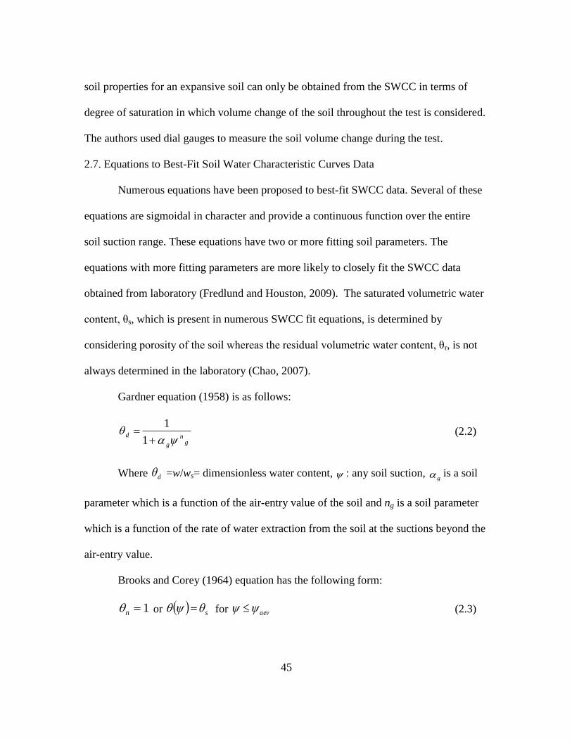
45
soil properties for an expansive soil can only be obtained from the SWCC in terms of
degree of saturation in which volume change of the soil throughout the test is considered.
The authors used dial gauges to measure the soil volume change during the test.
2.7. Equations to Best-Fit Soil Water Characteristic Curves Data
Numerous equations have been proposed to best-fit SWCC data. Several of these
equations are sigmoidal in character and provide a continuous function over the entire
soil suction range. These equations have two or more fitting soil parameters. The
equations with more fitting parameters are more likely to closely fit the SWCC data
obtained from laboratory (Fredlund and Houston, 2009). The saturated volumetric water
content, θs, which is present in numerous SWCC fit equations, is determined by
considering porosity of the soil whereas the residual volumetric water content, θr, is not
always determined in the laboratory (Chao, 2007).
Gardner equation (1958) is as follows:
gn
g
d
1
1 (2.2)
Where d =w/ws= dimensionless water content, : any soil suction, g is a soil
parameter which is a function of the air-entry value of the soil and ng is a soil parameter
which is a function of the rate of water extraction from the soil at the suctions beyond the
air-entry value.
Brooks and Corey (1964) equation has the following form:
1n or s for aev (2.3)
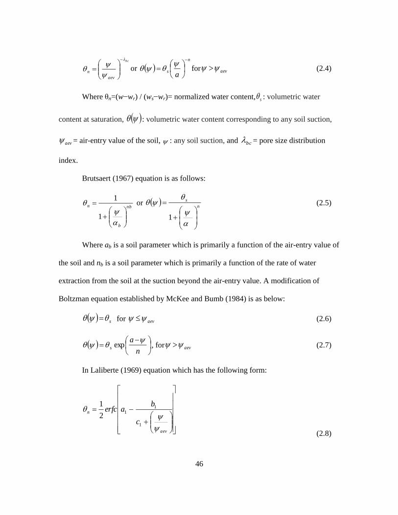
46
bc
aev
n
or
n
sa
for aev (2.4)
Where θn=(w−wr) / (ws−wr)= normalized water content, s : volumetric water
content at saturation, : volumetric water content corresponding to any soil suction,
aev = air-entry value of the soil, : any soil suction, and bc = pore size distribution
index.
Brutsaert (1967) equation is as follows:
nb
b
n
1
1 or
n
s
1
(2.5)
Where ab is a soil parameter which is primarily a function of the air-entry value of
the soil and nb is a soil parameter which is primarily a function of the rate of water
extraction from the soil at the suction beyond the air-entry value. A modification of
Boltzman equation established by McKee and Bumb (1984) is as below:
s for aev (2.6)
n
as
exp , for aev (2.7)
In Laliberte (1969) equation which has the following form:
aev
n
c
baerfc
1
11
2
1
(2.8)
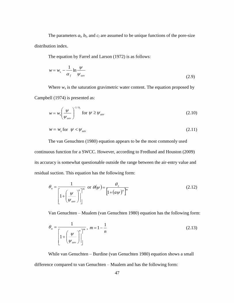
47
The parameters al, bl, and cl are assumed to be unique functions of the pore-size
distribution index.
The equation by Farrel and Larson (1972) is as follows:
aevf
sww
ln
1
(2.9)
Where ws is the saturation gravimetric water content. The equation proposed by
Campbell (1974) is presented as:
cb
aev
sww
/1
for aev (2.10)
sww for aev (2.11)
The van Genuchten (1980) equation appears to be the most commonly used
continuous function for a SWCC. However, according to Fredlund and Houston (2009)
its accuracy is somewhat questionable outside the range between the air-entry value and
residual suction. This equation has the following form:
mn
aev
n
1
1 or
mn
s
a
1 (2.12)
Van Genuchten – Mualem (van Genuchten 1980) equation has the following form:
mn
aev
n
1
1,
nm
11 (2.13)
While van Genuchten – Burdine (van Genuchten 1980) equation shows a small
difference compared to van Genuchten – Mualem and has the following form:
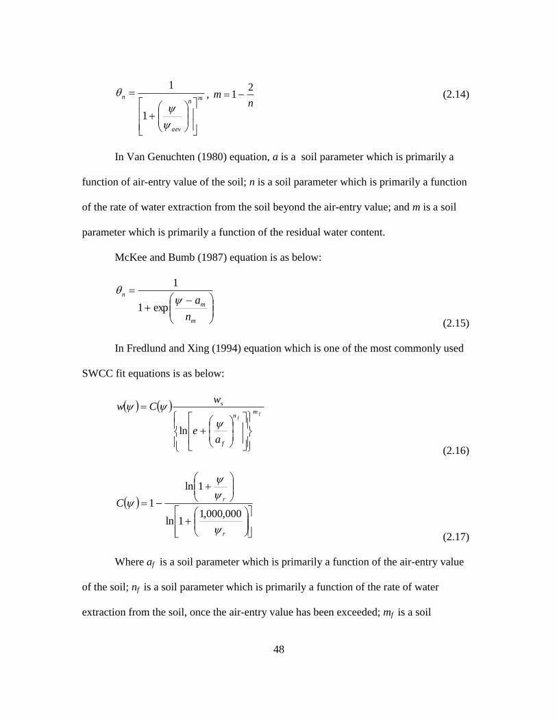
48
mn
aev
n
1
1,
nm
21 (2.14)
In Van Genuchten (1980) equation, a is a soil parameter which is primarily a
function of air-entry value of the soil; n is a soil parameter which is primarily a function
of the rate of water extraction from the soil beyond the air-entry value; and m is a soil
parameter which is primarily a function of the residual water content.
McKee and Bumb (1987) equation is as below:
m
m
n
n
a
exp1
1
(2.15)
In Fredlund and Xing (1994) equation which is one of the most commonly used
SWCC fit equations is as below:
f
f
mn
f
s
ae
wCw
ln
(2.16)
r
rC
000,000,1
1ln
1ln
1
(2.17)
Where af is a soil parameter which is primarily a function of the air-entry value
of the soil; nf is a soil parameter which is primarily a function of the rate of water
extraction from the soil, once the air-entry value has been exceeded; mf is a soil
49
parameter which is primarily a function of residual water content; and C is a
correction factor which is primarily a function of the suction at which residual water
content occurs. SWCC equation proposed by Fredlund and Xing (1994) uses a factor that
always directs the equation to a soil suction of 1,000,000 kPa at zero water content. This
equation can also be written as:
mn
aevwa
wa
s
uu
uue
wCw
ln
(2.18)
110
1ln
1ln
6
r
rC
(2.19)
where w = water content at any soil suction; C = correction factor
directing all SWCC curves to 1,000,000kPa at zero water content; r = residual suction;
aevwa uu = soil parameter indicating the inflection point that bears a relationship to the
air-entry value; n= soil parameter related to the rate of desaturation; and m= soil
parameter related to the curvature near residual conditions.
Feng and Fredlund (1999) equation is as below:
d
d
b
cabw
or
d
d
s
b
cb
(2.20)
Tani equation (Tani 1982) has the following form:
na
a
na
as
exp1
(2.21)
50
Fermi equation (McKee and Bumb 1987) is as below:
na
s
/exp1
(2.22)
Pereira and Fredlund (2000) equation has the following form:
ab
rs
r
c/1
(2.23)
Fredlund and Pham (Pham 2005) equation is as below:
r
r
rbr
c
cs w
a
aw
G
Cww
6101ln
1ln
1log
(2.24)
Mualem (1976) equation is:
cb
rsr
a
1 (2.25)
Williams, et al. (1983) equation has the following form:
lnln ba (2.26)
2.8. Use of Soil Water Characteristic Curves in Constitutive Relations for Unsaturated
Soils
Various empirical models and equations have been proposed for the estimation of
some of unsaturated soil property functions (e.g., unsaturated hydraulic conductivity,
shear strength, volume change). In each case, the estimation procedure involves the use
of the saturated soil properties in conjunction with the SWCC. This fact further
demonstrates the importance of SWCC in unsaturated soil mechanics. One of the major
51
used of SWCC is for estimation of unsaturated hydraulic conductivity functions of soils.
Some of the most common equations proposed by researchers use hydraulic conductivity
of the soil at full-saturation condition along with its SWCC in order to estimate the
unsaturated hydraulic conductivity function. The use of such equations has proven to be
of practical significance due to the fact that measurement of unsaturated hydraulic
conductivity of soils is a time-consuming and expensive procedure.
2.9. Models of Unsaturated Hydraulic Conductivity
The hydraulic conductivity of a saturated soil is typically considered to be
constant (McCartney et al. 2007). However, the hydraulic conductivity may change
drastically as the soil becomes unsaturated (i.e. suctions beyond the air-entry value).
The relationship between hydraulic conductivity and matric suction is usually
referred to as the kunsat-function and represents the change in the hydraulic conductivity
of the soil versus matric suction. Since volumetric moisture content (or degree of
saturation) of the soil is related to its matric suction (by SWCC), in some literature kunsat-
function curve may also be plotted as hydraulic conductivity versus volumetric moisture
content (or degree of saturation). In a saturated soil, all the pore spaces between the solid
particles are filled with water. Once the air-entry value is kunsat-function exceeded air
enters the largest pores and the air-filled pores become non conductive. This phenomenon
increases the tortuosity of the flow path. As a result, the ability of the soil to transport
water (i.e. the hydraulic conductivity of the soil) decreases (GEO-SLOPE International
Ltd., 2012).
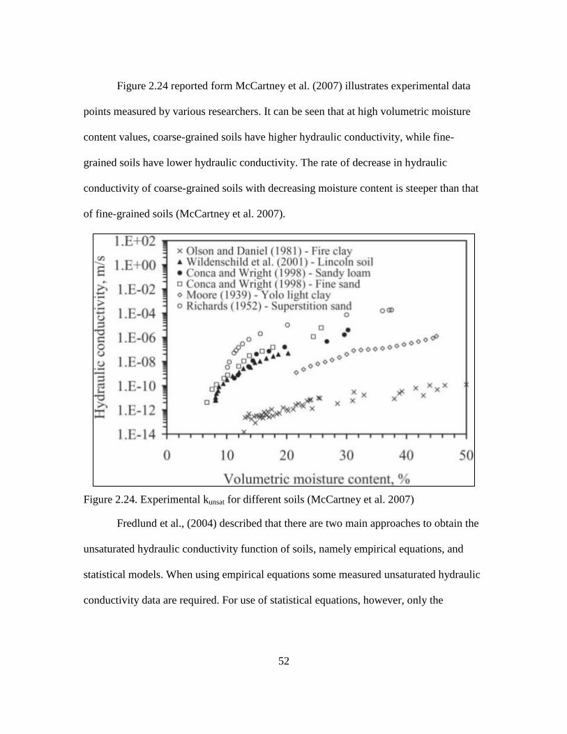
52
Figure 2.24 reported form McCartney et al. (2007) illustrates experimental data
points measured by various researchers. It can be seen that at high volumetric moisture
content values, coarse-grained soils have higher hydraulic conductivity, while fine-
grained soils have lower hydraulic conductivity. The rate of decrease in hydraulic
conductivity of coarse-grained soils with decreasing moisture content is steeper than that
of fine-grained soils (McCartney et al. 2007).
Figure 2.24. Experimental kunsat for different soils (McCartney et al. 2007)
Fredlund et al., (2004) described that there are two main approaches to obtain the
unsaturated hydraulic conductivity function of soils, namely empirical equations, and
statistical models. When using empirical equations some measured unsaturated hydraulic
conductivity data are required. For use of statistical equations, however, only the
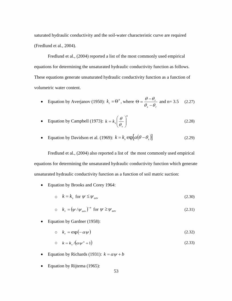
53
saturated hydraulic conductivity and the soil-water characteristic curve are required
(Fredlund et al., 2004).
Fredlund et al., (2004) reported a list of the most commonly used empirical
equations for determining the unsaturated hydraulic conductivity function as follows.
These equations generate unsaturated hydraulic conductivity function as a function of
volumetric water content.
Equation by Averjanov (1950): n
rk , where rs
r
and n= 3.5 (2.27)
Equation by Campbell (1973):
n
s
skk
(2.28)
Equation by Davidson et al. (1969): sskk exp (2.29)
Fredlund et al., (2004) also reported a list of the most commonly used empirical
equations for determining the unsaturated hydraulic conductivity function which generate
unsaturated hydraulic conductivity function as a function of soil matric suction:
Equation by Brooks and Corey 1964:
o skk for aev (2.30)
o n
aevrk
/ for aev (2.31)
Equation by Gardner (1958):
o exprk (2.32)
o 1/ n
skk (2.33)
Equation by Richards (1931): bk
Equation by Rijtema (1965):
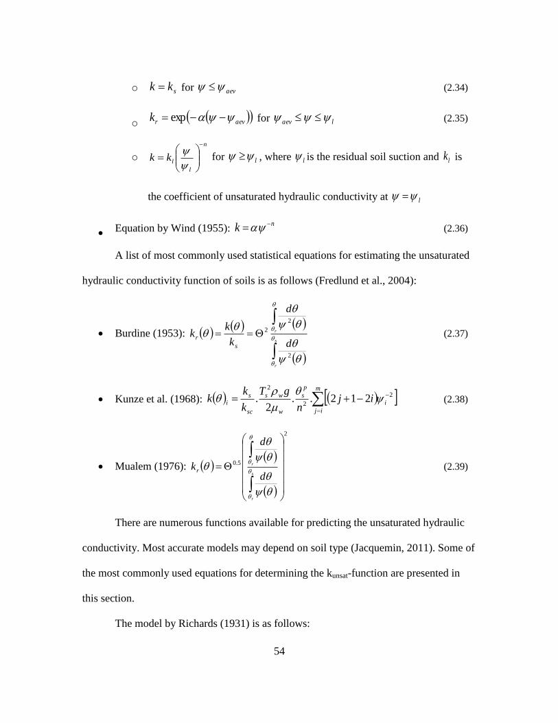
54
o skk for aev (2.34)
o aevrk exp for laev (2.35)
o
n
l
lkk
for l , where l is the residual soil suction and lk is
the coefficient of unsaturated hydraulic conductivity at l
Equation by Wind (1955): nk (2.36)
A list of most commonly used statistical equations for estimating the unsaturated
hydraulic conductivity function of soils is as follows (Fredlund et al., 2004):
Burdine (1953):
s
r
r
d
d
k
kk
s
r
2
2
2 (2.37)
Kunze et al. (1968):
m
ij
i
p
s
w
ws
sc
si ij
n
gT
k
kk 2
2
2
212..2
.
(2.38)
Mualem (1976):
2
5.0
s
r
r
d
d
kr
(2.39)
There are numerous functions available for predicting the unsaturated hydraulic
conductivity. Most accurate models may depend on soil type (Jacquemin, 2011). Some of
the most commonly used equations for determining the kunsat-function are presented in
this section.
The model by Richards (1931) is as follows:
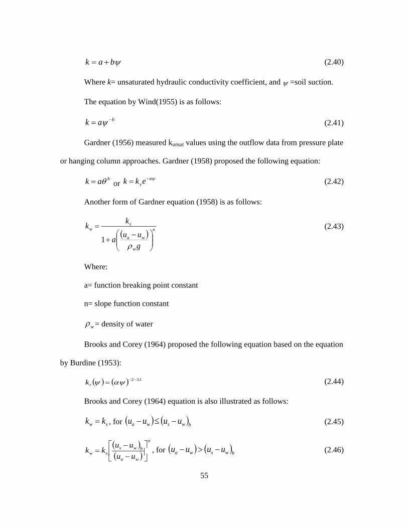
55
bak (2.40)
Where k= unsaturated hydraulic conductivity coefficient, and =soil suction.
The equation by Wind(1955) is as follows:
bak (2.41)
Gardner (1956) measured kunsat values using the outflow data from pressure plate
or hanging column approaches. Gardner (1958) proposed the following equation:
bak or a
sekk (2.42)
Another form of Gardner equation (1958) is as follows:
n
w
wa
sw
g
uua
kk
1
(2.43)
Where:
a= function breaking point constant
n= slope function constant
w = density of water
Brooks and Corey (1964) proposed the following equation based on the equation
by Burdine (1953):
32rk (2.44)
Brooks and Corey (1964) equation is also illustrated as follows:
sw kk , for bwswa uuuu (2.45)
n
wa
bws
swuu
uukk
, for
bwswa uuuu (2.46)
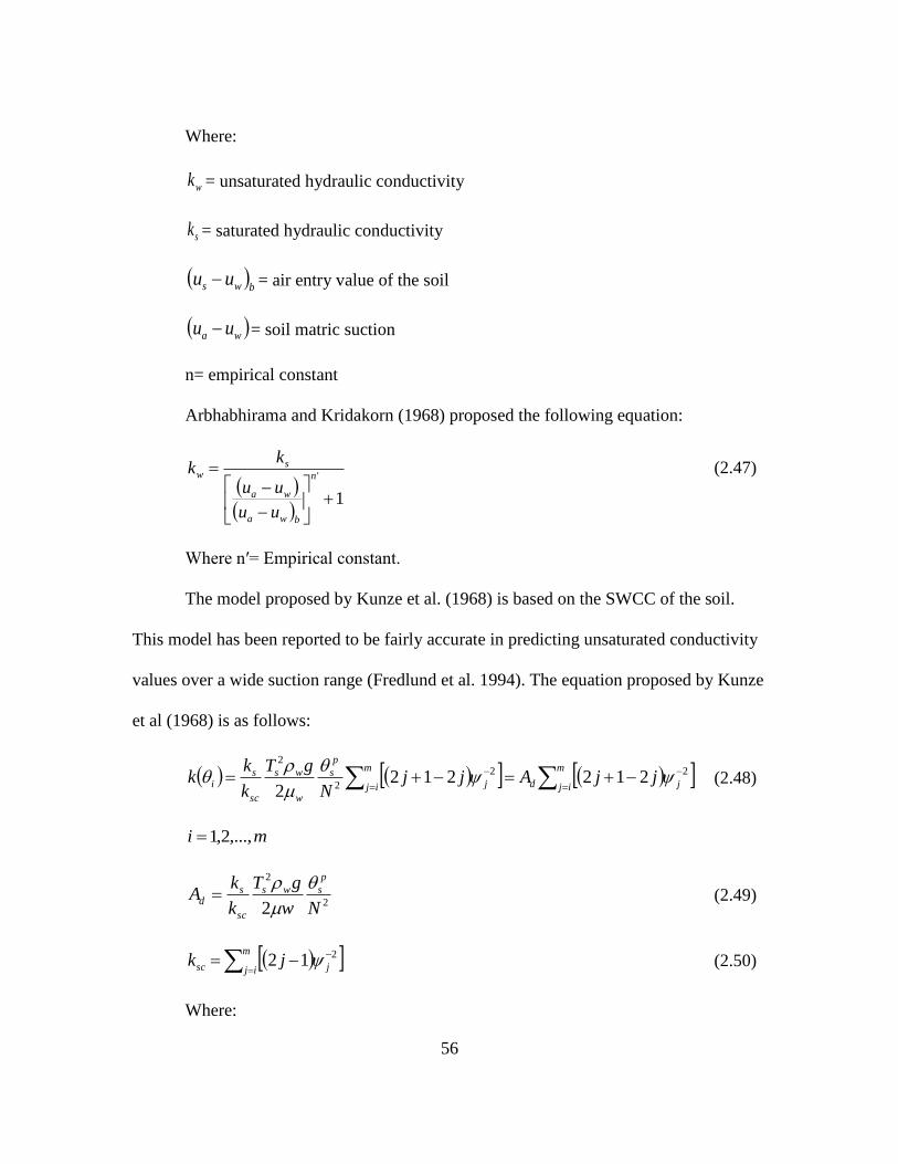
56
Where:
wk = unsaturated hydraulic conductivity
sk = saturated hydraulic conductivity
bws uu = air entry value of the soil
wa uu = soil matric suction
n= empirical constant
Arbhabhirama and Kridakorn (1968) proposed the following equation:
1
'
n
bwa
wa
sw
uu
uu
kk (2.47)
Where n′= Empirical constant.
The model proposed by Kunze et al. (1968) is based on the SWCC of the soil.
This model has been reported to be fairly accurate in predicting unsaturated conductivity
values over a wide suction range (Fredlund et al. 1994). The equation proposed by Kunze
et al (1968) is as follows:
m
ij j
m
ij dj
p
s
w
ws
sc
si jjAjj
N
gT
k
kk 22
2
2
2122122
(2.48)
mi ,...,2,1
2
2
2 Nw
gT
k
kA
p
sws
sc
sd
(2.49)
m
ij jsc jk 212 (2.50)
Where:

57
ik : Predicted hydraulic conductivity for a given volumetric water content
(m/s).
i: Interval number which increases as the volumetric water content decreases.
m: Total number of intervals between the saturated vol. water content and the
lowest volumetric water content.
sk : Measured saturated hydraulic conductivity (m/s).
sck : Saturated hydraulic conductivity or scaling factor (m/s).
dA : Adjusting constant.
sT : Surface tension of water (kN/m).
w : Water density (kg/m3).
g: Gravitational acceleration (m/s2).
w : Absolute viscosity of water (N s/m2).
s : Volumetric water content at S=1.0.
p: Pore size factor = 2 (Green and Corey, 1971)
N: Total number of intervals computed between the saturated volumetric water
content and the lowest water content.
j : Matric suction corresponding to the jth
interval (kPa)
Davidson et al.(1969) proposed the equation:
ss bkk exp (2.51)
Campbell (1973) equation is as follows:
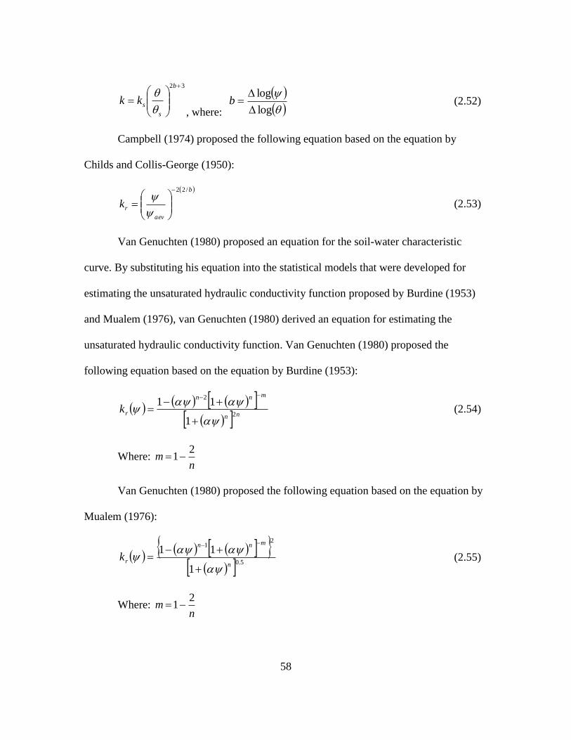
58
32
b
s
skk
, where:
log
log
b (2.52)
Campbell (1974) proposed the following equation based on the equation by
Childs and Collis-George (1950):
b
aev
rk
/22
(2.53)
Van Genuchten (1980) proposed an equation for the soil-water characteristic
curve. By substituting his equation into the statistical models that were developed for
estimating the unsaturated hydraulic conductivity function proposed by Burdine (1953)
and Mualem (1976), van Genuchten (1980) derived an equation for estimating the
unsaturated hydraulic conductivity function. Van Genuchten (1980) proposed the
following equation based on the equation by Burdine (1953):
nn
mnn
rk2
2
1
11
(2.54)
Where: n
m2
1
Van Genuchten (1980) proposed the following equation based on the equation by
Mualem (1976):
5.0
21
1
11
n
mnn
rk
(2.55)
Where: n
m2
1
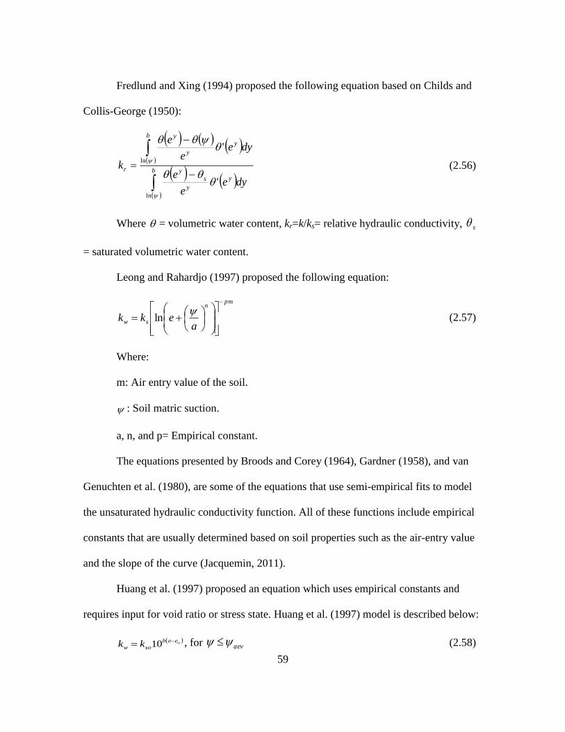
59
Fredlund and Xing (1994) proposed the following equation based on Childs and
Collis-George (1950):
b
y
y
s
y
b
y
y
y
r
dyee
e
dyee
e
k
ln
ln
'
'
(2.56)
Where = volumetric water content, kr=k/ks= relative hydraulic conductivity, s
= saturated volumetric water content.
Leong and Rahardjo (1997) proposed the following equation:
pmn
swa
ekk
ln (2.57)
Where:
m: Air entry value of the soil.
: Soil matric suction.
a, n, and p= Empirical constant.
The equations presented by Broods and Corey (1964), Gardner (1958), and van
Genuchten et al. (1980), are some of the equations that use semi-empirical fits to model
the unsaturated hydraulic conductivity function. All of these functions include empirical
constants that are usually determined based on soil properties such as the air-entry value
and the slope of the curve (Jacquemin, 2011).
Huang et al. (1997) proposed an equation which uses empirical constants and
requires input for void ratio or stress state. Huang et al. (1997) model is described below:
oeeb
sow kk
10 , for aev (2.58)
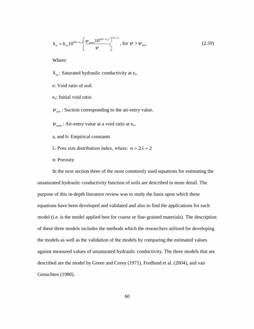
60
22
1010
o
o
eea
aevoeeb
sow kk , for aev (2.59)
Where:
sok : Saturated hydraulic conductivity at eo
e: Void ratio of soil.
eo: Initial void ratio.
aev : Suction corresponding to the air-entry value.
aevo : Air-entry value at a void ratio at eo.
a, and b: Empirical constants
λ: Pore size distribution index, where: 22 n
n: Porosity
In the next section three of the most commonly used equations for estimating the
unsaturated hydraulic conductivity function of soils are described in more detail. The
purpose of this in-depth literature review was to study the basis upon which these
equations have been developed and validated and also to find the applications for each
model (i.e. is the model applied best for coarse or fine-grained materials). The description
of these three models includes the methods which the researchers utilized for developing
the models as well as the validation of the models by comparing the estimated values
against measured values of unsaturated hydraulic conductivity. The three models that are
described are the model by Green and Corey (1971), Fredlund et al. (2004), and van
Genuchten (1980).
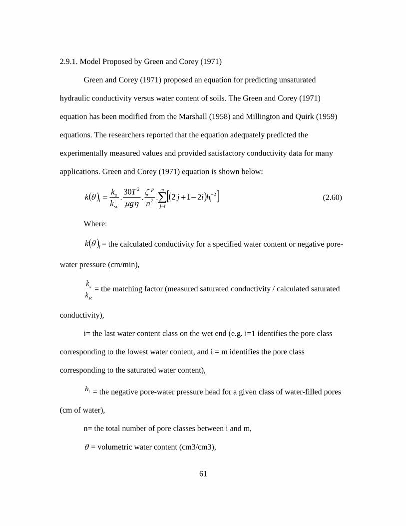
61
2.9.1. Model Proposed by Green and Corey (1971)
Green and Corey (1971) proposed an equation for predicting unsaturated
hydraulic conductivity versus water content of soils. The Green and Corey (1971)
equation has been modified from the Marshall (1958) and Millington and Quirk (1959)
equations. The researchers reported that the equation adequately predicted the
experimentally measured values and provided satisfactory conductivity data for many
applications. Green and Corey (1971) equation is shown below:
m
ij
i
p
sc
si hij
ng
T
k
kk 2
2
2
212..30
.
(2.60)
Where:
ik = the calculated conductivity for a specified water content or negative pore-
water pressure (cm/min),
sc
s
k
k= the matching factor (measured saturated conductivity / calculated saturated
conductivity),
i= the last water content class on the wet end (e.g. i=1 identifies the pore class
corresponding to the lowest water content, and i = m identifies the pore class
corresponding to the saturated water content),
ih = the negative pore-water pressure head for a given class of water-filled pores
(cm of water),
n= the total number of pore classes between i and m,
= volumetric water content (cm3/cm3),
62
T= surface tension of water (Dyn/cm),
= the water-saturated porosity,
= the viscosity of water (g/cm /s-1
),
g= the gravitational constant
= the density of water (g/cm3), and
p= a parameter that accounts for the interaction of pore classes
The following are some suggested values of ‘p’ given by various authors:
Marshall (1958): 2.0; Millington and Quirk (1961): 1.3; and Kunze et al. (1968): 1.0.
The shape of the conductivity function is controlled by the term (GeoStudio,
2012):
m
ij
ihij 2212 (2.61)
The term: 2
2
.30
ng
T p
is a constant for a particular function and can be taken to be
1.0 when determining the shape of the hydraulic conductivity function (GeoStudio,
2012). Green and Corey (1971) then compared some experimentally measured data on a
Guelph loam previously reported by Elrick and Bowman (1964) against hydraulic
conductivity values calculated by their proposed model, for which the authors reported
reliable predictions of the experimentally measured values.
Green and Corey (1971) also compared available measured hydraulic
conductivity data on glass beads from Topp and Miller (1966) against calculated values.
The authors matched the calculated curves at the saturated conductivity point and
reported adequate representation of the data.
63
Green and Corey (1971) also validated their model by comparing the calculated
values against previously measured hydraulic conductivity data by the following
researchers:
Topp (1969) experiment on desorption and adsorption cases on Rubicon sandy
loam
Green et al. (1964) experiment on an Iowas loess soil, Ida silt loam
Nielsen et al. (1964) experiment on Panoche clay loam obtained from different
depths
It should be mentioned that for all comparisons, the calculated and experimental
data were matched at s . All the curves were plotted in terms of hydraulic conductivity
versus volumetric moisture content ( ).
In case of Rubicon sandy loam, all of the computed curves for the adsorption case
were plotted beneath the measured hydraulic conductivities. Computed curves for
desorption case were within the envelope formed by the experimental values except at the
lower water contents. The agreement between measured and calculated data for Ida silt
loam was not as well as one for Guelph loam and glass beads.
Regarding comparing measured data provided by Nielsen et al. (1964) on
Panoche clay loam with calculated values using Green and Corey (1971) equation, some
of the plots showed good agreement while some other plots showed serious deviation of
calculated data from measured data. It should be noticed that unlike other comparisons,
the calculated and measured conductivities were matched at s = 0.35 cm3/cm
3 because
the saturated conductivity was not available.
64
2.9.2. Model Proposed by Fredlund et al. (2004)
Fredlund et al. (2004) proposed a model for estimating the unsaturated hydraulic
conductivity function which is an integration form of the suction versus water content
relationship. The authors also best fit the proposed equation to data obtained from the
literature where both the soil-water characteristic curve and the values of unsaturated
hydraulic conductivity were measured. The authors reported the fit between the measured
and estimated values to be excellent.
Fredlund et al. (2004) used equation by Kunze et al. (1968) and SWCC fitting
equation by Fredlund and Xing (1994) for the prediction of the unsaturated hydraulic
conductivity function of soils. Throughout the process, the authors assumed that the
volume change of the soil structure is negligible. The authors proposed the following
equation:
b
y
y
s
y
b
y
y
y
r
aev
dyee
e
dyee
e
k
ln
ln
'
'
(2.62)
Where:
b = ln(1,000,000), and
y is a dummy variable of integration representing the logarithm of suction.
Fredlund et al. (2004) compared between measured and predicted unsaturated hydraulic
conductivity values using their equation for five soils (shown in Table 2.4). The plots
showing this comparison are shown in Figures 2.25 through 2.29. The authors reported
that predicted and measured data show good agreement except for the data from Yolo
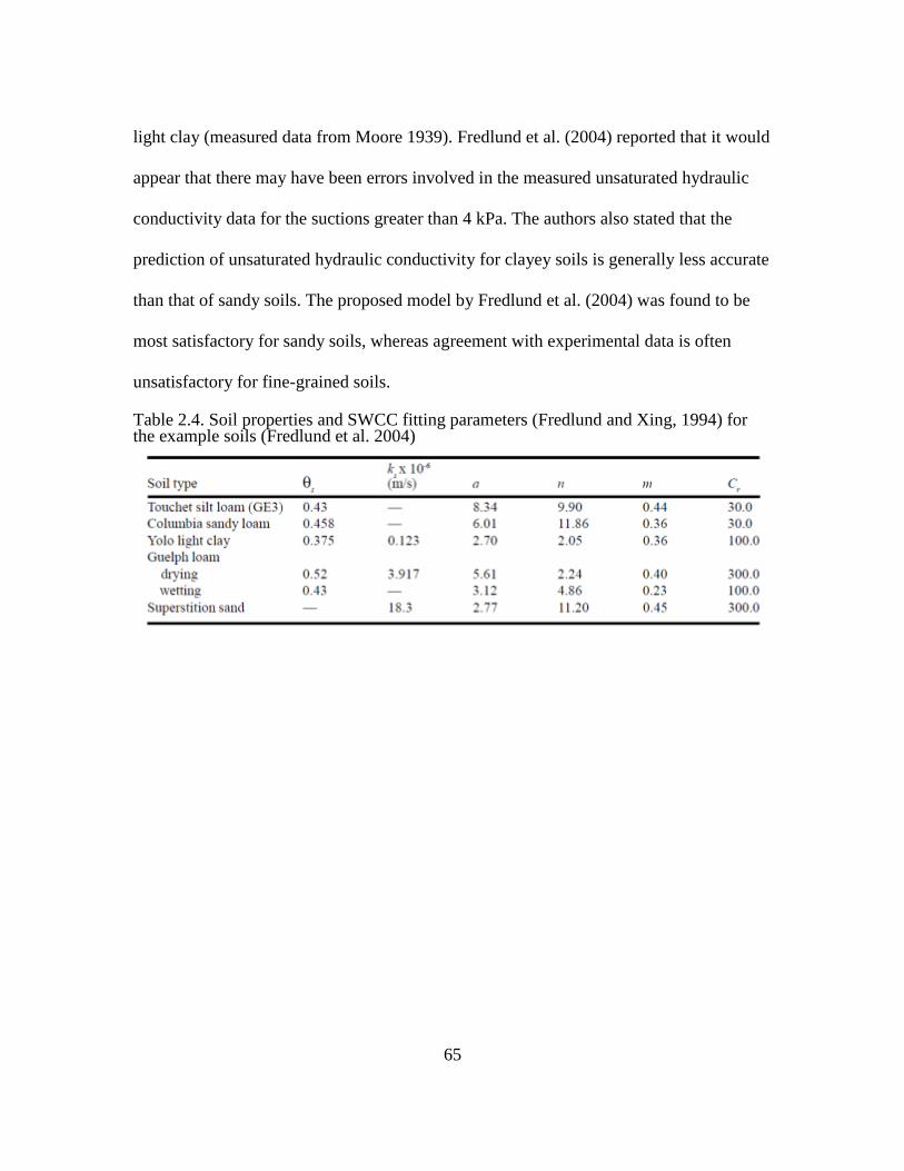
65
light clay (measured data from Moore 1939). Fredlund et al. (2004) reported that it would
appear that there may have been errors involved in the measured unsaturated hydraulic
conductivity data for the suctions greater than 4 kPa. The authors also stated that the
prediction of unsaturated hydraulic conductivity for clayey soils is generally less accurate
than that of sandy soils. The proposed model by Fredlund et al. (2004) was found to be
most satisfactory for sandy soils, whereas agreement with experimental data is often
unsatisfactory for fine-grained soils.
Table 2.4. Soil properties and SWCC fitting parameters (Fredlund and Xing, 1994) for the example soils (Fredlund et al. 2004)
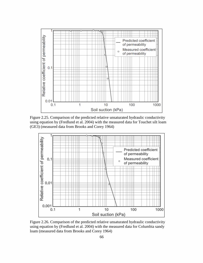
66
Figure 2.25. Comparison of the predicted relative unsaturated hydraulic conductivity
using equation by (Fredlund et al. 2004) with the measured data for Touchet silt loam
(GE3) (measured data from Brooks and Corey 1964)
Figure 2.26. Comparison of the predicted relative unsaturated hydraulic conductivity
using equation by (Fredlund et al. 2004) with the measured data for Columbia sandy
loam (measured data from Brooks and Corey 1964)
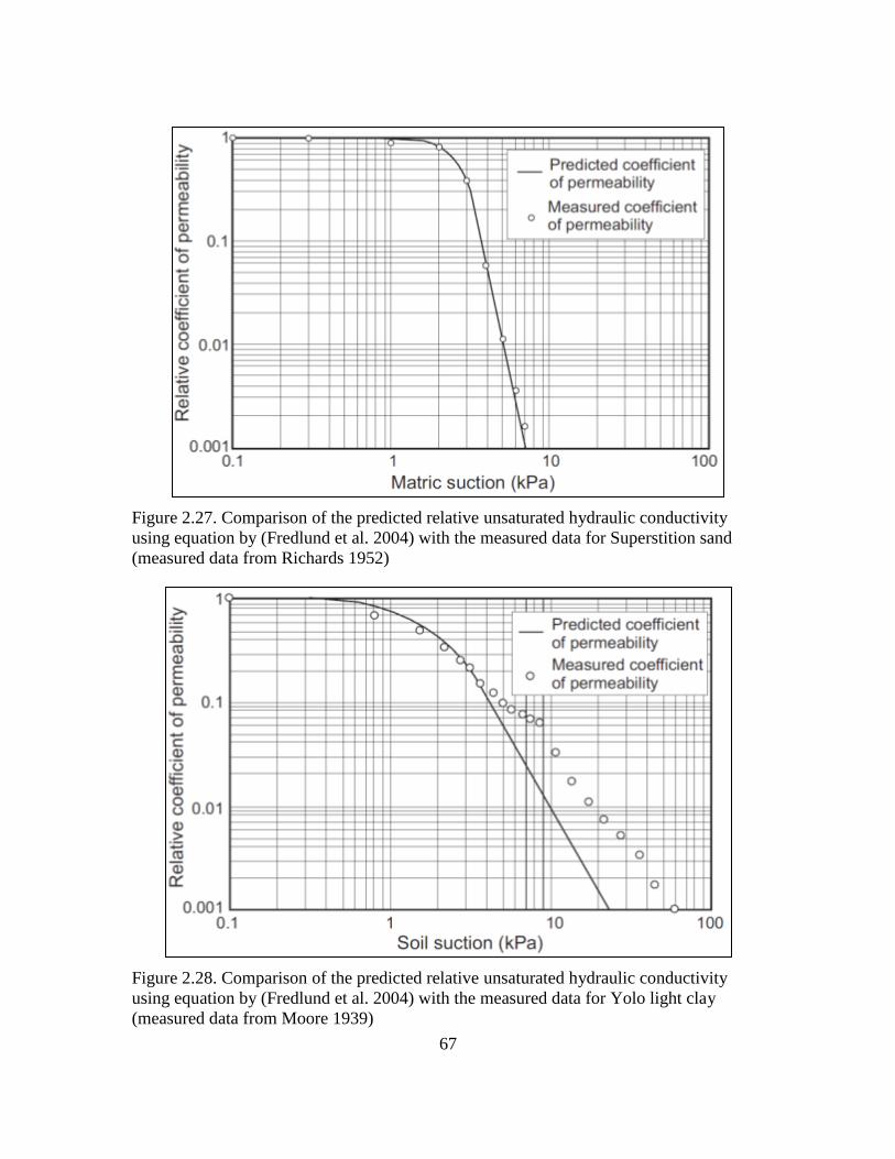
67
Figure 2.27. Comparison of the predicted relative unsaturated hydraulic conductivity
using equation by (Fredlund et al. 2004) with the measured data for Superstition sand
(measured data from Richards 1952)
Figure 2.28. Comparison of the predicted relative unsaturated hydraulic conductivity
using equation by (Fredlund et al. 2004) with the measured data for Yolo light clay
(measured data from Moore 1939)
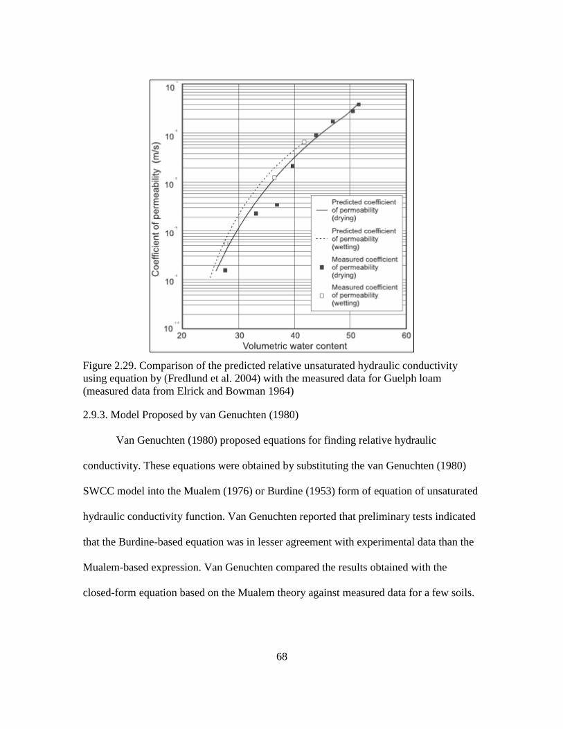
68
Figure 2.29. Comparison of the predicted relative unsaturated hydraulic conductivity
using equation by (Fredlund et al. 2004) with the measured data for Guelph loam
(measured data from Elrick and Bowman 1964)
2.9.3. Model Proposed by van Genuchten (1980)
Van Genuchten (1980) proposed equations for finding relative hydraulic
conductivity. These equations were obtained by substituting the van Genuchten (1980)
SWCC model into the Mualem (1976) or Burdine (1953) form of equation of unsaturated
hydraulic conductivity function. Van Genuchten reported that preliminary tests indicated
that the Burdine-based equation was in lesser agreement with experimental data than the
Mualem-based expression. Van Genuchten compared the results obtained with the
closed-form equation based on the Mualem theory against measured data for a few soils.
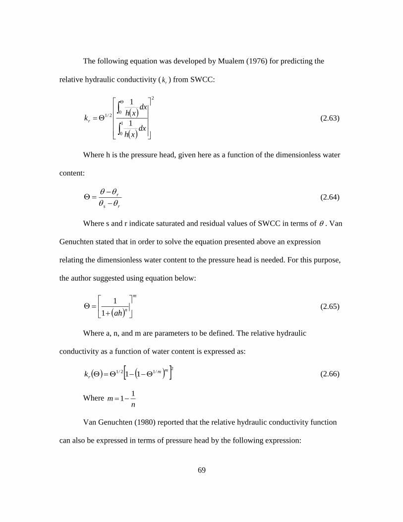
69
The following equation was developed by Mualem (1976) for predicting the
relative hydraulic conductivity (rk ) from SWCC:
2
1
0
02/1
1
1
dxxh
dxxh
kr (2.63)
Where h is the pressure head, given here as a function of the dimensionless water
content:
rs
r
(2.64)
Where s and r indicate saturated and residual values of SWCC in terms of . Van
Genuchten stated that in order to solve the equation presented above an expression
relating the dimensionless water content to the pressure head is needed. For this purpose,
the author suggested using equation below:
m
nah
1
1 (2.65)
Where a, n, and m are parameters to be defined. The relative hydraulic
conductivity as a function of water content is expressed as:
2/12/1 11mm
rk (2.66)
Where n
m1
1
Van Genuchten (1980) reported that the relative hydraulic conductivity function
can also be expressed in terms of pressure head by the following expression:
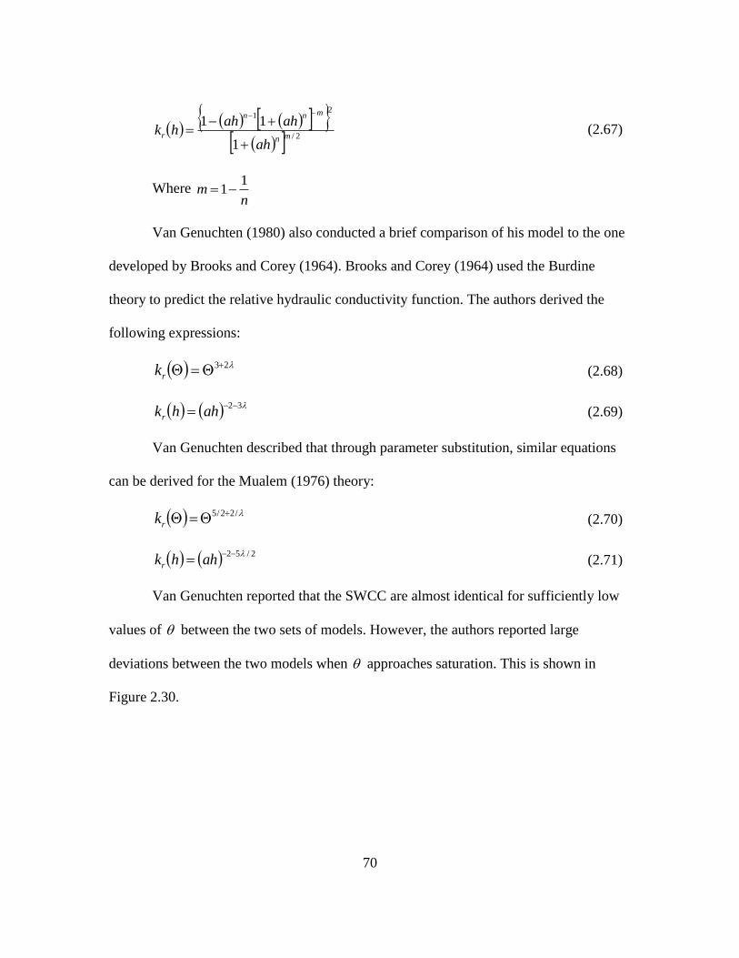
70
2/
21
1
11mn
mnn
r
ah
ahahhk
(2.67)
Where n
m1
1
Van Genuchten (1980) also conducted a brief comparison of his model to the one
developed by Brooks and Corey (1964). Brooks and Corey (1964) used the Burdine
theory to predict the relative hydraulic conductivity function. The authors derived the
following expressions:
23rk (2.68)
32 ahhkr (2.69)
Van Genuchten described that through parameter substitution, similar equations
can be derived for the Mualem (1976) theory:
/22/5 rk (2.70)
2/52 ahhkr (2.71)
Van Genuchten reported that the SWCC are almost identical for sufficiently low
values of between the two sets of models. However, the authors reported large
deviations between the two models when approaches saturation. This is shown in
Figure 2.30.
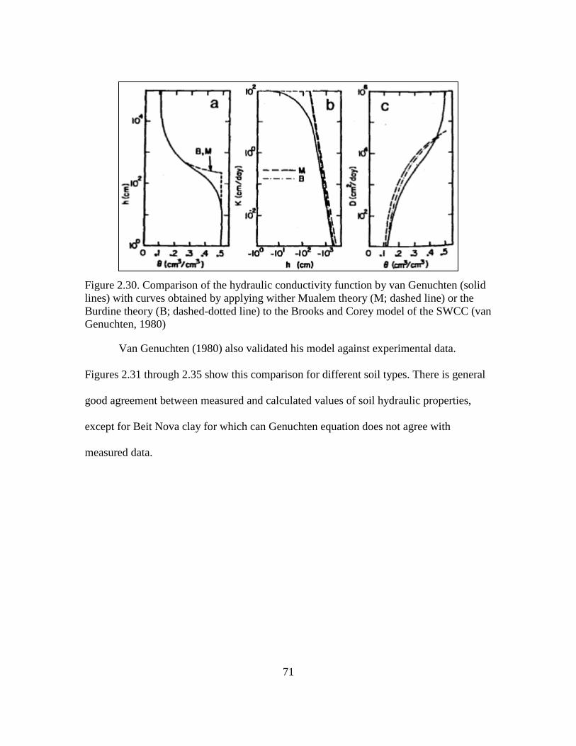
71
Figure 2.30. Comparison of the hydraulic conductivity function by van Genuchten (solid
lines) with curves obtained by applying wither Mualem theory (M; dashed line) or the
Burdine theory (B; dashed-dotted line) to the Brooks and Corey model of the SWCC (van
Genuchten, 1980)
Van Genuchten (1980) also validated his model against experimental data.
Figures 2.31 through 2.35 show this comparison for different soil types. There is general
good agreement between measured and calculated values of soil hydraulic properties,
except for Beit Nova clay for which can Genuchten equation does not agree with
measured data.
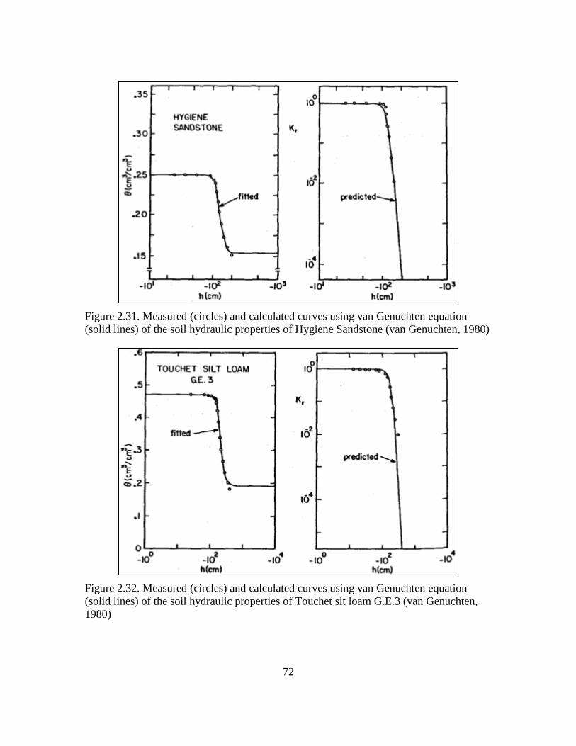
72
Figure 2.31. Measured (circles) and calculated curves using van Genuchten equation
(solid lines) of the soil hydraulic properties of Hygiene Sandstone (van Genuchten, 1980)
Figure 2.32. Measured (circles) and calculated curves using van Genuchten equation
(solid lines) of the soil hydraulic properties of Touchet sit loam G.E.3 (van Genuchten,
1980)
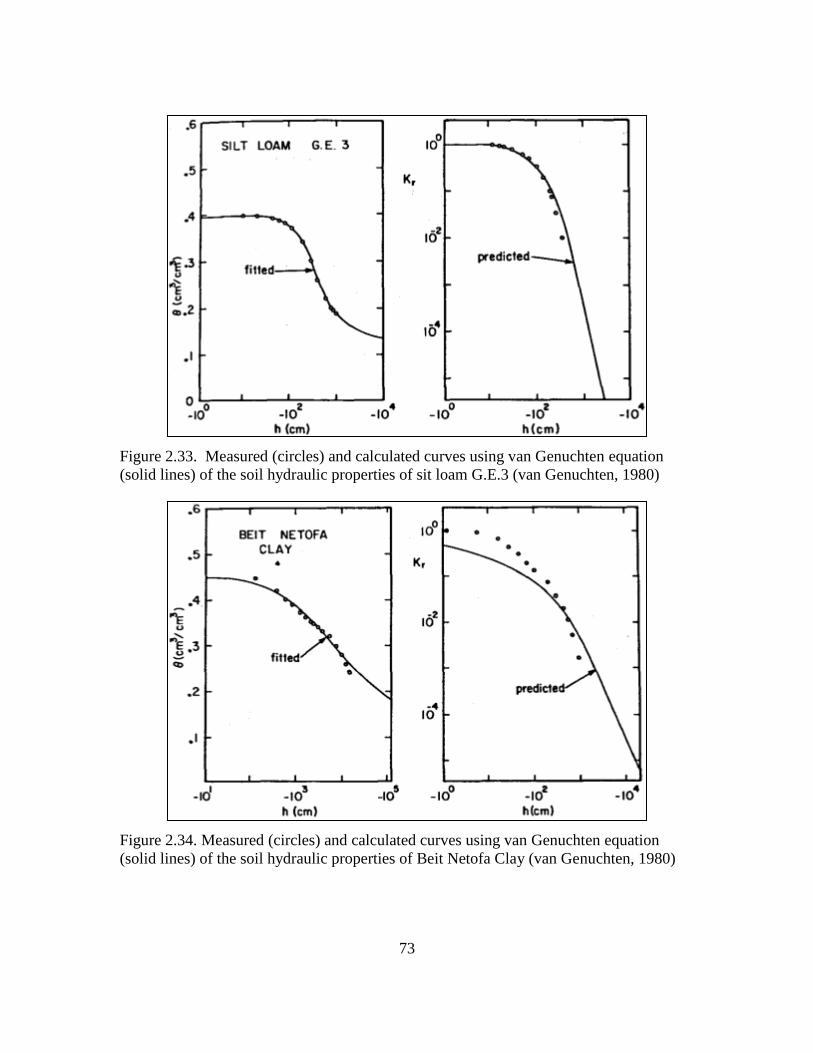
73
Figure 2.33. Measured (circles) and calculated curves using van Genuchten equation
(solid lines) of the soil hydraulic properties of sit loam G.E.3 (van Genuchten, 1980)
Figure 2.34. Measured (circles) and calculated curves using van Genuchten equation
(solid lines) of the soil hydraulic properties of Beit Netofa Clay (van Genuchten, 1980)
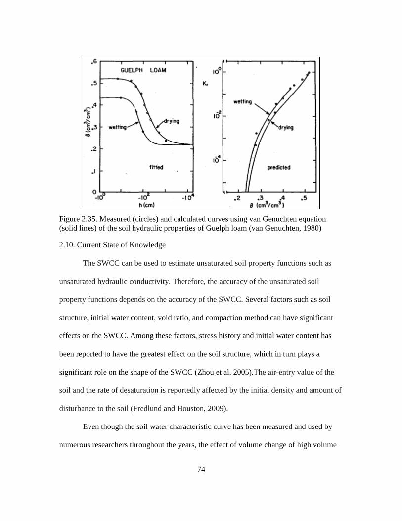
74
Figure 2.35. Measured (circles) and calculated curves using van Genuchten equation
(solid lines) of the soil hydraulic properties of Guelph loam (van Genuchten, 1980)
2.10. Current State of Knowledge
The SWCC can be used to estimate unsaturated soil property functions such as
unsaturated hydraulic conductivity. Therefore, the accuracy of the unsaturated soil
property functions depends on the accuracy of the SWCC. Several factors such as soil
structure, initial water content, void ratio, and compaction method can have significant
effects on the SWCC. Among these factors, stress history and initial water content has
been reported to have the greatest effect on the soil structure, which in turn plays a
significant role on the shape of the SWCC (Zhou et al. 2005).The air-entry value of the
soil and the rate of desaturation is reportedly affected by the initial density and amount of
disturbance to the soil (Fredlund and Houston, 2009).
Even though the soil water characteristic curve has been measured and used by
numerous researchers throughout the years, the effect of volume change of high volume
75
change soils (e.g. oil sands tailings, and expansive soils) has rarely been considered when
determining the SWCC's. This may lead to inaccurate SWCC's including the air-entry
value. Furthermore, it has been the common practice to estimate some of the major
unsaturated soil property functions (e.g., unsaturated hydraulic conductivity function,
shear strength) by using SWCC, which is a further support for recognizing the
importance of establishing true SWCC of high volume change soils. In recent years,
importance of considering the volume change of soils during suction change has been
recognized by a number of researchers; namely Salager et al. (2010), Pe´ron et al. (2007),
Nuth and Laloui (2011), Stange and Horn (2005), Mbonimpa et al. (2006), Perez-Garcia,
et al. (2008), and Fredlund and Houston, (2013).
Through literature study it was found that effect of net normal stress which is
applied to the soil specimen during the SWCC test, has also been under-studied. Only
very few researchers have conducted studies for finding the impact of net normal stress
on SWCC's (both drying and wetting cycles of SWCC) which in this research was found
to be important, particularly with regard to effect of net normal stress on volume change
of the soil during SWCC test on expansive clays. Furthermore, the effect of initial state of
the soil specimen including initial moisture content on SWCC has not been studied by a
lot of researchers. It is known that the initial condition of the soil (slurry versus
compacted at or near optimum moisture content) can have a significant effect on the
SWCC of the soil, particularly with regard to soil volume change (Fredlund, 2002).
Correction of SWCC's for soil volume change during the test may have a
considerable impact on air-entry value and shape of the SWCC. This, in turn, may have a
76
significant impact on unsaturated soil properties derived from the SWCC's (e.g. soil
hydraulic properties such as unsaturated hydraulic conductivity function). No studies on
numerical modeling of the effect of correction of SWCC for soil volume change on
hydraulic properties of the soils (e.g. advancement of wetted front) and its impact on
amount of suction-change induced deformation of expansive soils was found in the
literature.
An extensive literature review was conducted regarding the methods of SWCC
determination and the models available to best-fit the SWCC data obtained from
laboratory experiments. During this literature search SWCC's including typical air-entry
values and hysteresis were studied. Emphasis was placed upon the SWCC's of clays
because expansive clays were used as an example of high volume change soils for
purposes of this study on the effect of volume change on unsaturated soil properties and
flow-deformation. Use of soil water characteristic curves in constitutive relations for
unsaturated soils such as unsaturated hydraulic conductivity functions was also studied
through literature search. Some of the equations most commonly used to estimate
unsaturated hydraulic conductivity functions of soils based on the SWCC were studied.
This part of literature search included studying the methodologies used for developing the
equations for estimating unsaturated hydraulic conductivity functions as well as the
applications of the proposed equations. There are two main approaches to obtain the
unsaturated hydraulic conductivity function of soils, namely empirical equations, and
statistical models. When using empirical equations some measured unsaturated hydraulic
conductivity data are required. For use of statistical equations, however, only the
77
saturated hydraulic conductivity and the soil-water characteristic curve are required. It
was found that the most common equations used for estimating unsaturated hydraulic
conductivity functions of soils were developed for silts and sands. Undisturbed and
compacted specimens of silts and sands were used for developing or validating these
equations. Volume change of soils was not considered when developing these equations
and these equations work best for silts and sands and may not accurately estimate
unsaturated hydraulic conductivity functions of clays.
The importance of correcting SWCC's (including SWCC's in terms of volumetric
water content and degree of saturation) for soil volume change that occurs during the
SWCC test was studied through literature search. Additional literature search was carried
out to assess the effect of net normal stress on the shape of SWCC with regard to the soil
volume change throughout the test. Drying and wetting SWCC were studied through
literature search. Moreover, the importance of initial condition of the specimen (slurry
versus compacted specimen) was evaluated through literature search.
The literature review showed that slurry specimens undergo significant volume
change during SWCC test. Therefore, for a certain clayey soil the SWCC of the slurry
specimen may be different from that of the compacted specimen, not only because of
difference in soil structure but also due to large differences in volume change behavior.
The typical air-entry values of clays were studied through literature search. As
explained previously, air-entry value of a soil is defined as the matric suction at which
desaturation of the largest pores within the soil begins. The air-entry value of a specific
soil is related to the radius of the largest pore (i.e. if the largest pore is relatively small,
78
the air-entry value will be relatively large). Numerous researchers have found that the
saturation water content and air-entry value generally increases with the plasticity of the
soil (Fredlund and Xing, 1994). Fredlund (2011, 2013) reported that air-entry of soils is
generally quite close to their plastic limit. Consequently, the author concluded that there
is an approximate correlation between the plastic limit of a soil and its air-entry value.
Some other authors, however, reported different degrees of saturation (considerably less
than 100%) for soils at plastic limit (Ito and Azam, 2010, Li et al., 2009).
The hysteresis loop present between the wetting and drying paths of a SWCC was
also studied through literature search. Numerous researchers have measured SWCC's
including drying and wetting paths and presented the hysteresis associated with the
curves. It was found that at a given soil suction, the water content of the drying curve is
higher than that of the wetting curve (i.e. the drying curve lies above the wetting curve).
Furthermore, the end point of the wetting curve differs from the starting point of the
drying curve because of air entrapment in the soil. It was found from the literature search
that the wetting SWCC lies below the drying SWCC. Moreover, generally the end point
of the wetting curve is smaller than the starting point of the drying SWCC. This is
because some air becomes entrapped in the soil after it is wetted from a stress state in
excess of residual suction. Furthermore, the slope of the drying curve is approximately
parallel to that of the wetting curve.
The impact of net normal stress applied to the specimen during the SWCC test
was studied through literature search. Very limited data was found regarding effect of net
normal stress on the shape of the SWCC's. It was found that in general, stress history of

79
the applied normal stress does not seem to affect the shape of the SWCC significantly;
however, the AEV increases and the rate of degree of saturation change decreases with
increasing the net normal stress.
During the literature review, particular focus was placed upon studying whether in
common practice SWCC's are corrected for soil volume change. This was studied
particularly for the soils with high volume change potential. Suction induced volume
change in expansive soils occurs due to changes in the water content of the soil which
affects the stress equilibrium of the soil. Consequently, when determining the SWCC of
an expansive soil, it is important to consider the volume change that occurs as the suction
(and hence the water content of the soil) changes during the test (Chao et al., 2008). This
reportedly is not the common practice and the SWCC is usually measured assuming no
volume change of the soil specimen. This assumption is not correct for expansive soils.
When determining the SWCC of an expansive soil, it is important to consider the volume
change that occurs as the suction changes during the test (Chao et al. 2008). Soil water
characteristic curve fitting equations have been generated by a number of researchers
(e.g., Gardner 1956; Brooks and Corey 1964; van Genuchten 1980; Fredlund and Xing
1994). Although not always mentioned, the underlying assumption of most SWCC fitting
equations is that the soil is sufficiently stiff so that there is no change in void ratio of the
soil (i.e. soil volume change) during the test (Mbonimpa et al., 2006, Chiu and Ng, 2012).
Nonetheless, some of these equations have been extended for use in case of high volume
change materials. Pham and Fredlund (2008) proposed two SWCC equations for best-
fitting the SWCC for a wide range of soils types including high volume change clays. A
80
number of researchers have attempted to predict the SWCC's of expansive soils
(Chertkov 2004; Mbonimpa et al. 2006). It was found that in recent years a number of
researchers have recognized the importance of considering soil volume change when
establishing SWCC's. A number of researchers have conducted SWCC tests during which
the volume and mass of the specimen has been recorded and the volume change of the
specimen has been incorporated when generating the SWCC's. At the same time, the
measured data found on comparing volume change corrected and uncorrected SWCC's
was very limited and the researchers either reported the SWCC that is corrected for
volume change or the SWCC uncorrected for volume change.
A number of researchers recommended using degree of saturation SWCC as
opposed to gravimetric moisture content. The authors reported that when the soil
undergoes volume change during a suction increase, only the degree of saturation
variable clearly defines the air-entry value for the soil (as opposed to gravimetric and
volumetric water content).
Equations to best-fit soil water characteristic curves data were also studied
through literature search. Numerous equations have been proposed to best-fit SWCC
data. Several of these equations are sigmoidal in character and provide a continuous
function over the entire soil suction range. These equations have two or more fitting soil
parameters. The equations with more fitting parameters are more likely to closely fit the
SWCC data obtained from laboratory (Fredlund and Houston, 2009).
Various empirical models and equations have been proposed for the estimation of
some of unsaturated soil property functions (e.g., unsaturated hydraulic conductivity,
81
shear strength, volume change). In each case, the estimation procedure involves the use
of the saturated soil properties in conjunction with the SWCC. This fact further
demonstrates the importance of SWCC in unsaturated soil mechanics. One of the major
used of SWCC is for estimation of unsaturated hydraulic conductivity functions of soils.
Some of the most common equations proposed by researchers use hydraulic conductivity
of the soil at full-saturation condition along with its SWCC in order to estimate the
unsaturated hydraulic conductivity function. The use of such equations has proven to be
of practical significance due to the fact that measurement of unsaturated hydraulic
conductivity of soils is a time-consuming and expensive procedure. Numerous available
equation for estimating unsaturated hydraulic conductivity functions of soils were
studied. Three of the most commonly used equations for estimating the unsaturated
hydraulic conductivity function of soils were also described in more detail. The purpose
of this in-depth literature review was to study the basis upon which these equations have
been developed and validated and also to find the applications for each model (i.e. is the
model applied best for coarse or fine-grained materials). The description of these three
models includes the methods which the researchers utilized for developing the models as
well as the validation of the models by comparing the estimated values against measured
values of unsaturated hydraulic conductivity. The three models that are described are the
model by Green and Corey (1971), Fredlund et al. (2004), and van Genuchten (1980). It
was found that the underlying assumption for generating these equations have been that
the authors assumed that the volume change of the soil structure is negligible.
82
Chapter 3
LABORATORY TESTING
3.1. Introduction
The Soil Water Characteristic Curve (SWCC) describes the relationship between
either gravimetric water content, w, volumetric water content, θ , or degree of saturation,
S, and matric soil suction, (ua – uw), of the soil. The matric suction can be determined by
either a direct or indirect method. A direct measurement of matric suction is commonly
obtained with the axis translation technique. A common axis translation measurement
device is the pressure plate apparatus. An oedometer-type pressure plate device is one
common device used in geotechnical engineering to directly measure matric suction of
samples using the axis translation technique (Perera, et al., 2004).
In this study, a 1-D oedometer-type pressure plate device (i.e. SWC-150 device)
and the filter paper method were utilized to obtain the soil water characteristic curves for
expansive soils. The SWC-150 device is an oedometer-type pressure plate device that
was designed and manufactured by Geotechnical Consulting and Testing Systems, Inc.
(GCTS, 2004) and is an unsaturated soil testing apparatus with flexibility for controlling
the matric suction while applying various net normal stress values. The SWC-150
stainless steel SWCC apparatus allows use of a single soil specimen to obtain the entire
SWCC, up to the matric suction value of 1500 kPa (i.e., 15 bars), with any number of
equilibrium data points. This device can be used for determining SWCC of disturbed and
compacted (i.e. remolded specimens), initially slurried, or undisturbed specimens,
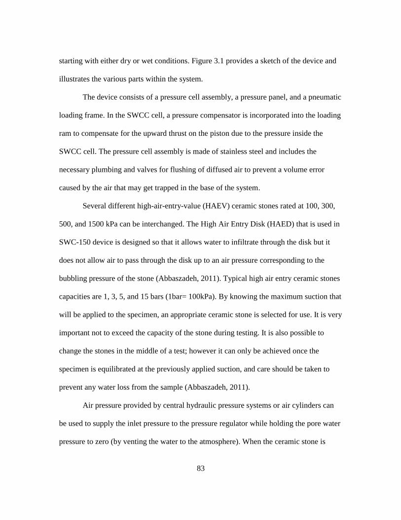
83
starting with either dry or wet conditions. Figure 3.1 provides a sketch of the device and
illustrates the various parts within the system.
The device consists of a pressure cell assembly, a pressure panel, and a pneumatic
loading frame. In the SWCC cell, a pressure compensator is incorporated into the loading
ram to compensate for the upward thrust on the piston due to the pressure inside the
SWCC cell. The pressure cell assembly is made of stainless steel and includes the
necessary plumbing and valves for flushing of diffused air to prevent a volume error
caused by the air that may get trapped in the base of the system.
Several different high-air-entry-value (HAEV) ceramic stones rated at 100, 300,
500, and 1500 kPa can be interchanged. The High Air Entry Disk (HAED) that is used in
SWC-150 device is designed so that it allows water to infiltrate through the disk but it
does not allow air to pass through the disk up to an air pressure corresponding to the
bubbling pressure of the stone (Abbaszadeh, 2011). Typical high air entry ceramic stones
capacities are 1, 3, 5, and 15 bars (1bar= 100kPa). By knowing the maximum suction that
will be applied to the specimen, an appropriate ceramic stone is selected for use. It is very
important not to exceed the capacity of the stone during testing. It is also possible to
change the stones in the middle of a test; however it can only be achieved once the
specimen is equilibrated at the previously applied suction, and care should be taken to
prevent any water loss from the sample (Abbaszadeh, 2011).
Air pressure provided by central hydraulic pressure systems or air cylinders can
be used to supply the inlet pressure to the pressure regulator while holding the pore water
pressure to zero (by venting the water to the atmosphere). When the ceramic stone is
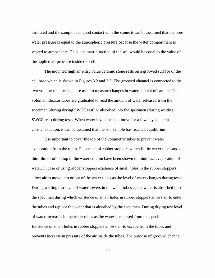
84
saturated and the sample is in good contact with the stone, it can be assumed that the pore
water pressure is equal to the atmospheric pressure because the water compartment is
vented to atmosphere. Thus, the matric suction of the soil would be equal to the value of
the applied air pressure inside the cell.
The mounted high air entry value ceramic stone rests on a grooved surface of the
cell base which is shown in Figures 3.2 and 3.3. The grooved channel is connected to the
two volumetric tubes that are used to measure changes in water content of sample. The
volume indicator tubes are graduated to read the amount of water released from the
specimen (during drying SWCC test) or absorbed into the specimen (during wetting
SWCC test) during tests. When water level does not move for a few days under a
constant suction, it can be assumed that the soil sample has reached equilibrium.
It is important to cover the top of the volumetric tubes to prevent water
evaporation from the tubes. Placement of rubber stoppers which fit the water tubes and a
thin film of oil on top of the water column have been shown to minimize evaporation of
water. In case of using rubber stoppers existence of small holes in the rubber stoppers
allow air to move into or out of the water tubes as the level of water changes during tests.
During wetting test level of water lowers in the water tubes as the water is absorbed into
the specimen during which existence of small holes in rubber stoppers allows air to enter
the tubes and replace the water that is absorbed by the specimen. During drying test level
of water increases in the water tubes as the water is released from the specimen.
Existence of small holes in rubber stoppers allows air to escape from the tubes and
prevents increase in pressure of the air inside the tubes. The purpose of grooved channel
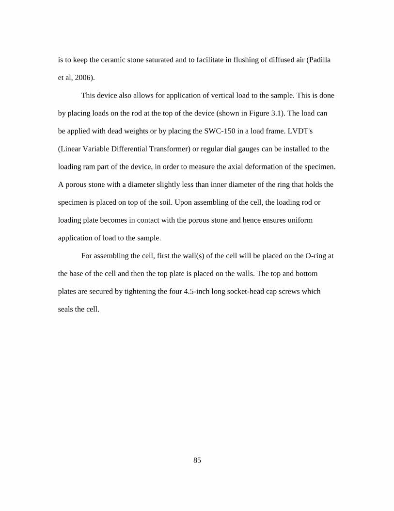
85
is to keep the ceramic stone saturated and to facilitate in flushing of diffused air (Padilla
et al, 2006).
This device also allows for application of vertical load to the sample. This is done
by placing loads on the rod at the top of the device (shown in Figure 3.1). The load can
be applied with dead weights or by placing the SWC-150 in a load frame. LVDT's
(Linear Variable Differential Transformer) or regular dial gauges can be installed to the
loading ram part of the device, in order to measure the axial deformation of the specimen.
A porous stone with a diameter slightly less than inner diameter of the ring that holds the
specimen is placed on top of the soil. Upon assembling of the cell, the loading rod or
loading plate becomes in contact with the porous stone and hence ensures uniform
application of load to the sample.
For assembling the cell, first the wall(s) of the cell will be placed on the O-ring at
the base of the cell and then the top plate is placed on the walls. The top and bottom
plates are secured by tightening the four 4.5-inch long socket-head cap screws which
seals the cell.
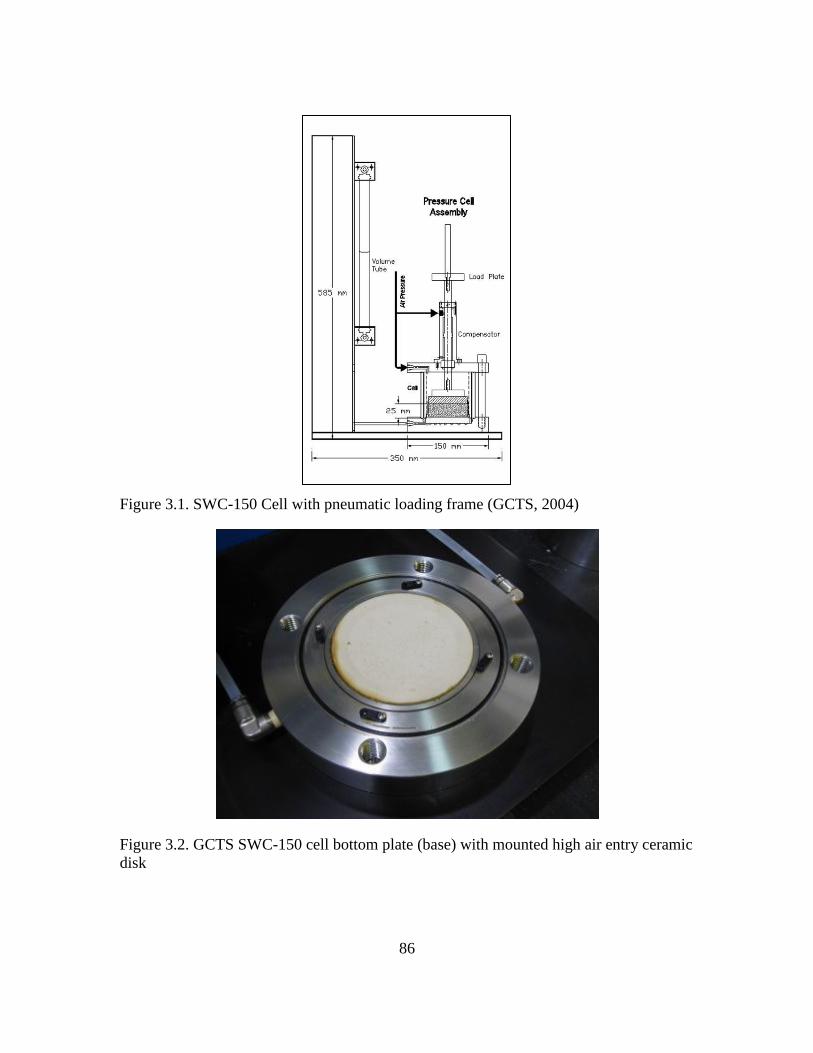
86
Figure 3.1. SWC-150 Cell with pneumatic loading frame (GCTS, 2004)
Figure 3.2. GCTS SWC-150 cell bottom plate (base) with mounted high air entry ceramic
disk
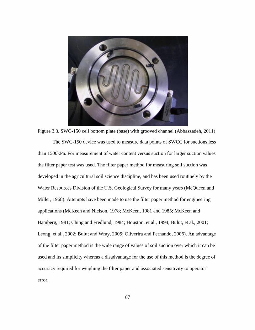
87
Figure 3.3. SWC-150 cell bottom plate (base) with grooved channel (Abbaszadeh, 2011)
The SWC-150 device was used to measure data points of SWCC for suctions less
than 1500kPa. For measurement of water content versus suction for larger suction values
the filter paper test was used. The filter paper method for measuring soil suction was
developed in the agricultural soil science discipline, and has been used routinely by the
Water Resources Division of the U.S. Geological Survey for many years (McQueen and
Miller, 1968). Attempts have been made to use the filter paper method for engineering
applications (McKeen and Nielson, 1978; McKeen, 1981 and 1985; McKeen and
Hamberg, 1981; Ching and Fredlund, 1984; Houston, et al., 1994; Bulut, et al., 2001;
Leong, et al., 2002; Bulut and Wray, 2005; Oliverira and Fernando, 2006). An advantage
of the filter paper method is the wide range of values of soil suction over which it can be
used and its simplicity whereas a disadvantage for the use of this method is the degree of
accuracy required for weighing the filter paper and associated sensitivity to operator
error.
88
The principle of the filter paper method is that the suction of a filter paper will
come to equilibrium with that of the soil sample. The relative humidity inside the
container which holds the soil and filter paper will be controlled by the soil suction.
Equilibrium can be reached by either liquid or vapor moisture exchange between the
filter paper and the soil specimen. By using the filter paper method it is possible to
measure either the total or the matric suction of a soil (ASTM D5298-94). When the filter
paper is placed in contact with the water in the soil, the soil suction measured at
equilibrium will be the matric suction of the soil, because the salt content of the water in
the filter paper will be the same as that of the soil water (Chao, 2007).
In this method, a specimen of the soil along with a calibrated filter paper is placed
in a closed container. Filter paper tests for measuring soil suction must be conducted with
great care in order to minimize error and obtain accurate results. It has been found to be
critical that the specimens for filter paper test should be placed and kept in a temperature-
controlled environment (Jacquemin, 2011). The soil sample and the filter paper are
allowed to equilibrate for a period of time at a constant temperature.
3.2. Laboratory Tests Performed
As a part of this study, Soil Water Characteristic Curves (SWCC) of three clays,
Anthem, Colorado, and San Antonio, were determined. The tested soils have different
clay mineralogies and variable degrees of swell potentials. Points on the SWCC in the
low range of suction (below 1,500kPa) were obtained using the SWC-150. For suction
values greater than 1,500 kPa, points on the SWCC were determined using the filter
paper test.
89
During this study, the effect of the initial state of the sample including its initial
moisture content on the SWCC was studied. For this purpose, slurry specimens and
compacted specimens (prepared at 95% of maximum standard dry density compacted at
optimum moisture content) were prepared and tested and the results were compared
against each other.
Also the effect of volume change of expansive clays on their SWCC was studied.
It was found that volume change that occurs during suction change under applied load
can be significant, and affects the SWCC, including key features of the SWCC such as
the AEV. The impacts of volume change on AEV have been previously discussed by
Fredlund and Houston (2013). Taking the soil volume change into account, therefore,
may lead to more accurate estimation of soil properties such as shear strength and
hydraulic conductivity when these unsaturated soil properties are estimated using
saturated property measurements plus the SWCC (Fredlund et al. 2003).
As another part of this study, the effect of net normal stress upon the SWCC of
the samples was evaluated. For this purpose, SWCC's of soil specimens prepared at the
same initial density and moisture content (95% of maximum standard dry density and
optimum moisture content) were measured under different net normal stress values. The
values of applied net normal stresses were: 7kPa, ~25%, and ~50% of the swell pressure
of the soil. Furthermore, SWCC's including drying and wetting curves for different net
normal stress values were measured and analyzed. In the following sections, basic
properties of the test soils used in this study are presented.
90
3.3. Soils Used in the Laboratory Testing Program
Three clays were tested as a part of this study. These soils were collected from
Arizona, Colorado, and Texas and are referred to as Anthem, Colorado, and San Antonio
soils in this study. Basic properties of these soils were determined at Arizona State
University by a research team and the data are shown in Table 3.1 and Figures 3.4
through 3.6. Natural moisture content, for shallow deposit field conditions, were 6% for
Anthem and Colorado, and 5% for San Antonio. ASTM Standards used are:
ASTM D6913 - 04(2009) Particle-Size Distribution) Using Sieve Analysis
ASTM D422 - 63(2007) Particle-Size Distribution) Using Hydrometer Test
ASTM D698 - 12– Standard test Methods for Laboratory Compaction
Characteristics of Soils Using Standard Efforts
ASTM D854 - 10– Standard Test Methods for Specific Gravity of Soil Solids by
Water Pycnometer
ASTM D4318 - 10– Standard Test Methods for Liquid Limit, Plastic Limit, and
Plasticity Index of Soil
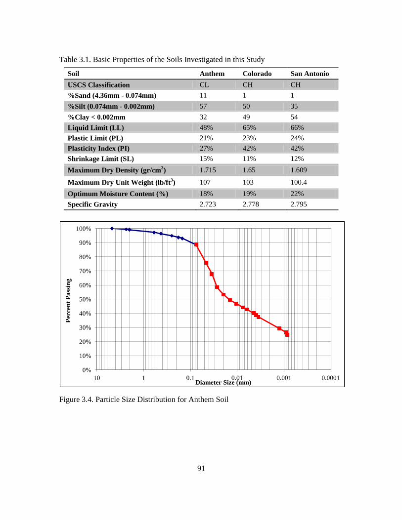
91
Table 3.1. Basic Properties of the Soils Investigated in this Study
Soil Anthem Colorado San Antonio
USCS Classification CL CH CH
%Sand (4.36mm - 0.074mm) 11 1 1
%Silt (0.074mm - 0.002mm) 57 50 35
%Clay < 0.002mm 32 49 54
Liquid Limit (LL) 48% 65% 66%
Plastic Limit (PL) 21% 23% 24%
Plasticity Index (PI) 27% 42% 42%
Shrinkage Limit (SL) 15% 11% 12%
Maximum Dry Density (gr/cm3) 1.715 1.65 1.609
Maximum Dry Unit Weight (lb/ft3) 107 103 100.4
Optimum Moisture Content (%) 18% 19% 22%
Specific Gravity 2.723 2.778 2.795
Figure 3.4. Particle Size Distribution for Anthem Soil
0%
10%
20%
30%
40%
50%
60%
70%
80%
90%
100%
0.0001 0.001 0.01 0.1 1 10
Per
cen
t P
ass
ing
Diameter Size (mm)
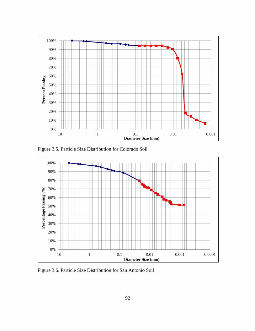
92
Figure 3.5. Particle Size Distribution for Colorado Soil
Figure 3.6. Particle Size Distribution for San Antonio Soil
0%
10%
20%
30%
40%
50%
60%
70%
80%
90%
100%
0.001 0.01 0.1 1 10
Per
cen
t P
ass
ing
Diameter Size (mm)
0%
10%
20%
30%
40%
50%
60%
70%
80%
90%
100%
0.0001 0.001 0.01 0.1 1 10
Per
cen
tag
e P
ass
ing
(%
)
Diameter Size (mm)
93
3.4. Soil Water Characteristic Tests
3.4.1 SWCC Determination Using 1-D Oedometer Pressure Plate Cells
Table 3.2 shows the list of SWCC tests conducted as a part of this study. A total
of 21 SWCC tests were performed. Compacted specimens of Anthem, Colorado, and San
Antonio soils were prepared by compacting the soil at 95% standard maximum dry
density and at optimum moisture content. Due to high plasticity of soils in this study,
existence of clods was noticed upon wetting of the soil. As an attempt to break the clods
using mortar and pestle, the soils were pulverized and passed through US No. 100 sieve.
However, it was noticed that clods would re-appear when water was added to the soil to
reach the optimum moisture content. The required quantity of distilled water was added
to the soils using a spray bottle to reach the water content to optimum. Afterwards, the
soil was sealed in plastic bags and left for at least 15 days for equilibrium. The longer
duration required for equilibrium was due to fine-grained particles of the soil and its high
plasticity. After equilibrium was reached, the soil was compacted in three layers into
standard SWCC brass rings at 95% maximum dry density.
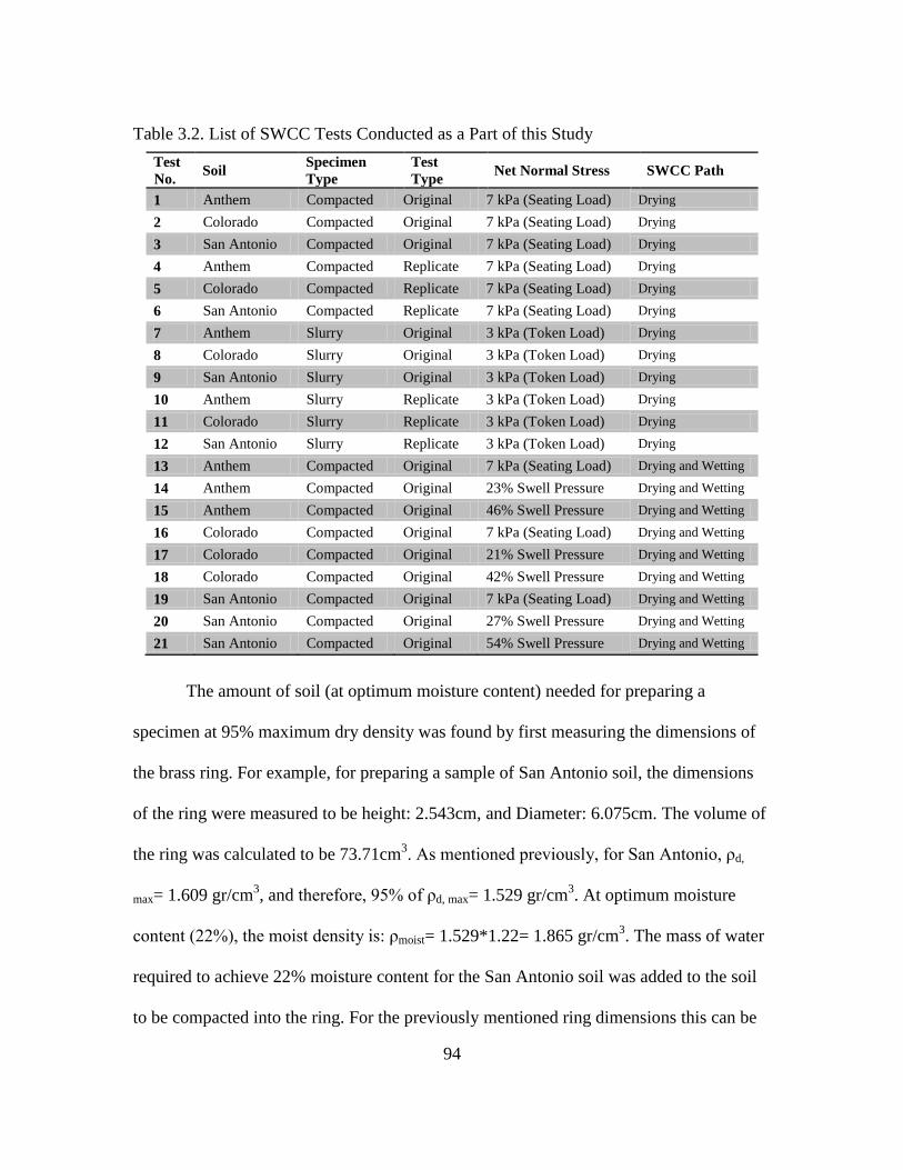
94
Table 3.2. List of SWCC Tests Conducted as a Part of this Study
Test
No. Soil
Specimen
Type
Test
Type Net Normal Stress SWCC Path
1 Anthem Compacted Original 7 kPa (Seating Load) Drying
2 Colorado Compacted Original 7 kPa (Seating Load) Drying
3 San Antonio Compacted Original 7 kPa (Seating Load) Drying
4 Anthem Compacted Replicate 7 kPa (Seating Load) Drying
5 Colorado Compacted Replicate 7 kPa (Seating Load) Drying
6 San Antonio Compacted Replicate 7 kPa (Seating Load) Drying
7 Anthem Slurry Original 3 kPa (Token Load) Drying
8 Colorado Slurry Original 3 kPa (Token Load) Drying
9 San Antonio Slurry Original 3 kPa (Token Load) Drying
10 Anthem Slurry Replicate 3 kPa (Token Load) Drying
11 Colorado Slurry Replicate 3 kPa (Token Load) Drying
12 San Antonio Slurry Replicate 3 kPa (Token Load) Drying
13 Anthem Compacted Original 7 kPa (Seating Load) Drying and Wetting
14 Anthem Compacted Original 23% Swell Pressure Drying and Wetting
15 Anthem Compacted Original 46% Swell Pressure Drying and Wetting
16 Colorado Compacted Original 7 kPa (Seating Load) Drying and Wetting
17 Colorado Compacted Original 21% Swell Pressure Drying and Wetting
18 Colorado Compacted Original 42% Swell Pressure Drying and Wetting
19 San Antonio Compacted Original 7 kPa (Seating Load) Drying and Wetting
20 San Antonio Compacted Original 27% Swell Pressure Drying and Wetting
21 San Antonio Compacted Original 54% Swell Pressure Drying and Wetting
The amount of soil (at optimum moisture content) needed for preparing a
specimen at 95% maximum dry density was found by first measuring the dimensions of
the brass ring. For example, for preparing a sample of San Antonio soil, the dimensions
of the ring were measured to be height: 2.543cm, and Diameter: 6.075cm. The volume of
the ring was calculated to be 73.71cm3. As mentioned previously, for San Antonio, ρd,
max= 1.609 gr/cm3, and therefore, 95% of ρd, max= 1.529 gr/cm
3. At optimum moisture
content (22%), the moist density is: ρmoist= 1.529*1.22= 1.865 gr/cm3. The mass of water
required to achieve 22% moisture content for the San Antonio soil was added to the soil
to be compacted into the ring. For the previously mentioned ring dimensions this can be
95
calculated to be: Mass of 22% moist soil needed for ring 1: 1.865 (gr/cm3)*73.71 (cm
3) =
137.47 gr.
Specimens were compacted into brass rings with height of ~2.5 cm and diameter
of ~6.4 cm in three layers. Each layer was prepared with soil weighing one third of the
total targeted weight of the soil specimen for the ring. Top surfaces of the two bottom
compacted layers were scarified using a sharp-edged tool to establish good contact
between the soil layers. The height of each layer was kept to one third of the ring height.
A steel rod with diameter of about 18 mm was used for compaction to achieve a dry
density of 95% standard maximum dry unit weight of soil.
At least two replicates of each test were run on specimens prepared from the same
soil. The purpose of running replicate tests was to achieve higher reliability in test results
and to better know measurement scatter through generating more data points. After
preparation, compacted specimens were soaked in water to reach saturation (or close to
saturation) condition. Due to the fact that the soils tested were all expansive clays, in
order to minimize swell during specimen soaking, some seating load was applied to the
specimens. The amount of net normal stress applied was around 15kPa. The specimens
were soaked for a few days (6 to 10 days). Saturated specimens were then taken out of
water and the excess water was mopped from exterior of the ring using a paper towel and
the mass of saturated soil plus ring was recorded. After measuring the saturated mass of
the specimen, the specimen was ready to start the test.
For the low range of suction (lower than 1500kPa) the test was carried out in the
SWC-150 oedometer-pressure plate cells (GCTS, 2004). This apparatus, as mentioned
96
previously, uses axis translation method to control matric suction. Air pressure provided
by central hydraulic pressure system (for air pressures up to 700kPa) or air cylinders (for
air pressures up to 1500kPa) was used to supply the inlet pressure to the pressure
regulator while holding the pore water pressure to zero. By this method matric suction
values of up to 1500kPa were achieved.
At the beginning and throughout the test, the water in the tubes (which was
distilled and de-aired water) was flushed using a flushing device to expel any trapped air
in the groove at the bottom of the cell (underneath the high air entry stone). While
flushing, care was taken not to introduce more air into the grooves located in the bottom
plate and also not to spill any water from the top of the tubes. When no more air bubbles
were observed during flushing, the device was assumed to be ready to use and the test
was started by applying the desired net normal stress and cell pressure (i.e. suction).
The tests in this study were generally started at matric suction of 10kPa to 25kPa.
The saturated specimens were set in the device (at the center of the HAEV ceramic stone)
and the device was assembled and the net normal stress and suction were applied to the
specimen. Net normal stress was applied by putting weights on the loading ram which is
located at the top of the cell. The specimens were allowed to equilibrate at each suction
value, which due to high plasticity and low permeability of the soils took about one
month (for each suction point). During this time water levels in the tubes were monitored
and if no change in water level was noticed for 5 to 7 days, it was assumed that the
sample has reached equilibrium. At this point, the air pressure was released and the
SWCC device was dismantled (in drying SWCC paths) and the specimen was weighed
97
and any deformation (axial and radial) was measured by use of electronic calipers. For
the cases in which SWCC device was not dismantled (e.g. at low suctions during wetting
cycles when the only volume change was axial due to large net normal stress values
which minimized the radial shrinkage of the soil), the volume change of the soil
specimen was measured by use of dial gauges installed at the top of the device, and the
amount of water released from the specimen (or absorbed into the specimen) was
measured by monitoring the levels of water in the tubes.
For the cases with low suction (200kPa or less, and depending on the applied net
normal stress) when the full contact between the soil and ring was maintained, the cell
was not disassembled. This was due to the fact that there was no radial shrinkage of the
specimen and it was assumed that the volume change of the sample was only in the
vertical direction. For these cases only the water level change was monitored for water
content determination (i.e. no direct measurement of the mass of the specimen was made
after equilibration) and vertical deformation of the soil was measured using dial gauges.
It should be mentioned that under high values of suction (greater than 200kPa)
particularly for the tests with smaller net normal stresses, it was noticed that the soil
tended to pull away slightly from the ring (i.e. radial shrinkage due to drying) and
therefore, volume change of the soil was both radial and vertical. For these cases the cells
were dismantled after equilibration and the radial and axial deformations were
determined by calipers.
At the end of the last pressure increment, the pressure was released and the
apparatus was disassembled. Following measurement of the weight and dimensions of
98
specimen, the specimen was kept in the oven for drying for at least 24 hours at 110 ºC
and its dry weight was recorded. The obtained data was used to determine volumetric
water content, degree of saturation, and gravimetric water content of the soil specimens
for different suction values.
The gravimetric water content was found by determining the mass of water and
solids by over drying the soil. By definition, gravimetric water content is the ratio of the
mass of water to the dry mass of soil:
s
w
M
Mw (3.1)
Where w is the gravimetric water content, wM is the mass of water present in the
soil, and sM is the mass of solids. Degree of saturation is the ratio of volume of water to
the volume of voids:
v
w
V
VS (3.2)
Where S is the degree of saturation, wV is the volume of water, and vV is the
volume of voids. Degree of saturation can also be calculated by using the following
equations:
1
d
ws
s
G
wGS
(3.3)
Where sG is the specific gravity of the soil, w is the water content, w is the unit
weight of water, and d is the dry unit weight of the soil. As mentioned previously,
specific gravities of the Anthem, Colorado, and San Antonio soils and are listed in Table
99
3.1. The dry density of the specimens was also calculated for each suction tested by
measuring the volume and mass of the specimen. This data was used for each suction
tested to find the degree of saturation of the specimen.
In order to evaluate importance of volume change measurement in determining
SWCC's, the degree of saturation of the soils were once calculated based on the initial
volume of the specimen (i.e. the volume of the specimen at the time of starting the
SWCC test). The values of degrees of saturation of the specimens were also calculated
based on the instantaneous volume of the specimen, which is the true volume of
specimen at the time of equilibrium at each suction. For determining the instantaneous
volume of the specimen the amount of radial and/or axial deformation was taken into
account. The SWCC's that were generated based on the instantaneous volume of the
specimen are referred to as volume corrected SWCC's and the SWCC's that were
generated based on the initial volume of the specimen (i.e. volume change of the
specimen throughout the test was not considered in determining the SWCC) are referred
to as volume uncorrected SWCC's.
Volumetric water content is defined as the ratio of volume of water to the total
volume of the specimen:
vs
w
T
w
VV
V
V
V
(3.4)
Where is the volumetric water content, wV is the volume of water, sV is the
volume of solids, vV is the volume of voids, and TV is the total volume of the specimen.
The equations for volumetric water content can also be written as:
100
w
dw
(3.5)
Values of water content and d were known for the specimen equilibrated at
certain suction values. Similar to calculating degree of saturation, volumetric water
content for each suction was calculated once based on the initial volume of the specimen
(i.e. ignoring volume change of the specimen throughout the test) and once based on the
instantaneous volume of the specimen which was determined by measuring radial and
axial deformations of the specimen by using calipers. The SWCC in terms of volumetric
water content that was generated based on the initial volume of the specimen is referred
to as volume uncorrected SWCC and the one generated based on the instantaneous
volume of the specimen is referred to as volume corrected SWCC. The results of the
SWCC tests are presented later in this chapter.
The slurry specimens were made by first measuring the mass of the ring. The ring
was then set on top of the High Air Entry Disk (HAED) of SWCC device. HAED was
kept saturated prior to starting of the test. Pulverized soil at natural moisture content was
then added to the ring with a small compaction effort until the ring was filled with soil.
The mass of soil added to the ring was determined by weighing the soil container before
and after putting soil in the ring. When the ring was filled with soil water was added very
slowly allowing the water to penetrate into the soil and fill the ring uniformly. The mass
of added water was also measured by knowing the mass of water container before and
after putting water in the ring. By knowing the dimensions of the ring and mass of soil,
the soil moisture content, and mass of water, the dry and wet density of soil in the ring
101
was calculated and used for determining volumetric water content and degree of
saturation values for each suction.
Similar to SWCC tests for compacted specimens, slurry specimens were allowed
to equilibrate at each suction value. Also a token load (≈7kPa) was applied to the
specimens. The purpose of the token load is that it helps provide a positive contact
between the soil specimen and the ceramic stone for efficient water migration to and from
the soil specimen. Due to high volume change of slurry specimens, upon equilibration at
each suction, the SWCC cell was dismantled and the soil specimen was weighed and its
volume change (axial and radial deformation) was measured by calipers when there was
sample shrinkage. At the end of each test, the samples were weighed and volume changes
were measured and recorded and the samples were dried in an oven with temperature of
110⁰C for 16 to 20 hours in order to calculate the final water content of the soil. The
obtained data was used to compute the required parameters such as volumetric water
content, and degree of saturation. Appendix A includes some of the images of the
compacted and slurry specimens equilibrated at different suction values tested in this
study. The images illustrate volume change of soils throughout the tests.
3.4.2 SWCC Determination Using Filter Paper Test
The SWCC data points for larger suction range (greater than 1,500kPa) were
measured by filter paper. For the filter paper test in this study, Whatman’s No. 42 filter
paper was used. The filter paper tests were conducted in accordance to the article titled
“Laboratory Filter Paper Suction Measurements” (Houston, Houston and Wagner, 1994).
102
A filter paper in contact with the soil specimens allows water in the liquid phase
and solutes to exchange freely and therefore, measures matric suction (Rahardjo and
Leong, 2006). A total of two filter papers were used in each of the filter paper tests. The
soil was compacted at 95% maximum dry density and the filter papers were placed in
between the layer of the soil to ensure close contact between soil and filter paper. At least
one month was allowed for matric suction equilibrium.
In the filter paper tests for this study, whenever handling the filter papers, latex
gloves were worn to avoid contamination of the filter papers to dust or any residue. The
filter papers were cut into small pieces. The small pieces of filter paper were then
wrapped inside clean filter papers to avoid direct contact between the soil and the small
piece of filter paper. Filter paper was then placed in between compacted layers of soil
(compacted at 95% maximum dry density and at different moisture contents) in glass jars.
The surface of soil where the filter paper was placed was scarified to ensure good contact
between the soil and the filter paper.
The filter papers within the soil was allowed time to equilibrate to the soil
moisture content for the duration of about one month and then the filter papers were
taken out and weighed and the moisture content was determined by oven drying. When
the filter paper was to be removed and weighed, the soil around the filter paper was first
removed. For this portion of the test also, latex gloves were used to avoid contamination
of filter papers. The filter paper was carefully removed from the soil and immediately
placed in a plastic bag with previously measured mass. The bag containing the filter
paper was weighed and then the piece of filter paper was dried in an oven at a
103
temperature of 110⁰C for 24 hours. The dry mass of filter paper was then determined and
the moisture content of the filter paper was calculated. All of the weights (expect
specimen weight) were measured using a scale with 10-4
grams accuracy.
The filter paper water content was then related to the soil matric suction. The
moisture content of the soil taken out of the jar was also determined. In order to increase
the accuracy of test results, two or three measurements of water contents and suction
were taken from each jar (at various locations within the jar). The relationship between
the filter paper water content and the soil matric suction is specific to the type of filter
paper used. Since Whatman’s No. 42 filter paper was used, the following relationship
was used (Chandler and Gutierrez, 1986):
rfilterpapewpF 0622.0850.5 (3.6)
pF
wkPa 10 (3.7)
Where:
pF : Soil matric suction in pF
kPa : Soil matric suction in kPa
rfilterpapew : Filter paper water content
w : Unit weight of water
With the wet and dry mass of filter papers, the correlation above can be used to
determine the matric suction of the soil within which the filter paper has been placed
previously. The results of filter paper test are presented in the following sections.
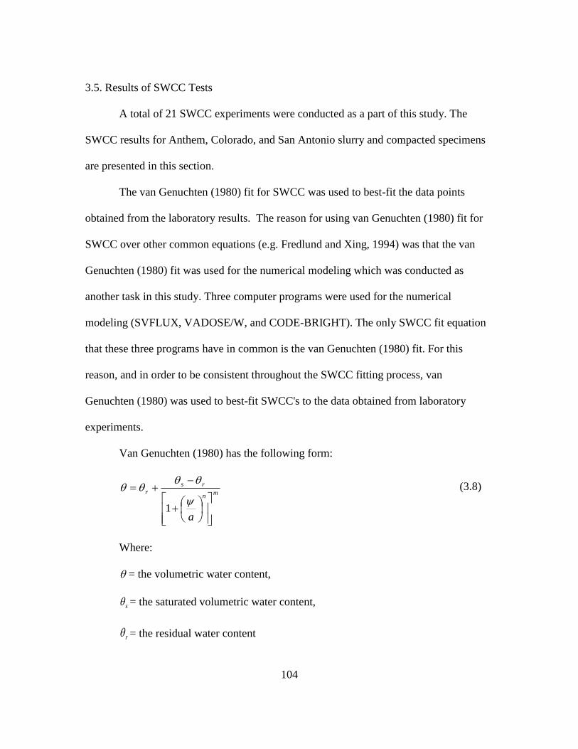
104
3.5. Results of SWCC Tests
A total of 21 SWCC experiments were conducted as a part of this study. The
SWCC results for Anthem, Colorado, and San Antonio slurry and compacted specimens
are presented in this section.
The van Genuchten (1980) fit for SWCC was used to best-fit the data points
obtained from the laboratory results. The reason for using van Genuchten (1980) fit for
SWCC over other common equations (e.g. Fredlund and Xing, 1994) was that the van
Genuchten (1980) fit was used for the numerical modeling which was conducted as
another task in this study. Three computer programs were used for the numerical
modeling (SVFLUX, VADOSE/W, and CODE-BRIGHT). The only SWCC fit equation
that these three programs have in common is the van Genuchten (1980) fit. For this
reason, and in order to be consistent throughout the SWCC fitting process, van
Genuchten (1980) was used to best-fit SWCC's to the data obtained from laboratory
experiments.
Van Genuchten (1980) has the following form:
mn
rs
r
a
1
(3.8)
Where:
= the volumetric water content,
s = the saturated volumetric water content,
r = the residual water content
105
= the negative pore-water pressure (i.e. matric suction), and
a, n, m = curve fitting parameters
"a" has units of pressure and corresponds to the air-entry value of the SWCC (i.e.
larger "a" indicates larger AEV's). "a" has also been defined as the pivot point about
which the "n" parameter changes the slope of the function (Geo-Slope, 2012). "n"
corresponds to the slope of the curve, i.e. larger values of "n" indicate larger slope of the
curve in the region between the air-entry value and the residual suction. "m" is related to
"n" with the expression: n
nm
1
The parameter m affects the sharpness of the sloping portion of the curve as it
enters the lower plateau (Geo-Slope, 2012). The same form of van Genuchten equation
can be applied to the SWCC's in terms of gravimetric water content and degree of
saturation. Van Genuchten (1980) equation for SWCC in terms of degree of saturation
(S) is as below:
mn
rsr
a
SSSS
1
(3.9)
Throughout the following sections, SWCC data points obtained from laboratory
tests are presented along with the best-fit curve using van Genuchten equation. The
values of van Genuchten equation parameters (a, n, and m) are also presented for each
SWCC in order to make the necessary comparisons.
106
3.5.1. SWCC of Compacted Specimens
Compacted specimens of Anthem, Colorado, and San Antonio soils were prepared
and tested under net normal stress of 7kPa (seating load). The purpose of this set of
testing was to find the impact of soil volume change on the shape of the SWCC's, with
particular focus on the air-entry values and slope in the transition zone.
The SWCC plots show that the compacted specimens never achieved complete
saturation even upon complete submergence (due to the presence of occluded air-
bubbles). On other words, 100% saturation was not obtained when soaking the specimens
under water (with load on the top of specimens). It should also be mentioned that at the
end of wetting tests, 100% saturation was not obtained due to presence of occluded air-
bubbles.
Two replicate specimens of each soil, which were prepared at the same density
and water content, were tested in order to find the reproducibility and reliability of
results. The results that are shown in Figures 3.7 through 3.15 suggest good
reproducibility of tests.
Table 3.3 contains the list of van Genuchten SWCC fit parameters for the SWCC
tests conducted on compacted specimens of Anthem, Colorado, and San Antonio soils.
The applied net normal stress in this series of tests was 7kPa (i.e. seating load). A seating
load was used to ensure good contact between the specimen and the high air-entry stone
throughout the test. As shown in the Table 3.3, for a certain soil, values of "a" are larger
for the SWCC's in terms of volumetric water content and degree of saturation compared
to the "a" for SWCC's in terms of gravimetric water content. The is due to the fact that
107
the SWCC's in terms of volumetric water content and degree of saturation are corrected
for soil volume change that occurred throughout the test. The soils tested in this study are
expansive soils which shrink upon drying (i.e. increase in suction). This leads to decrease
in volume of the specimen which is in fact decrease in the volume of voids as the soil
particles are assumed to stiff enough so that no volume change of the soil particles occurs
during the change in suction. As described in earlier sections of this chapter volumetric
water content and degree of saturation of soils are defined by the following equations:
vs
w
T
w
VV
V
V
V
(3.10)
v
w
V
VS (3.11)
It can be found from these equations that for a certain amount of water, a decrease
in volume of voids will lead to larger values of volumetric water content and degree of
saturation. Therefore, at a certain suction, SWCC that has been corrected for soil volume
change generally shows larger values of volumetric water content and degree of
saturation. At the same time, the soil volume change cannot be incorporated in the SWCC
in terms of gravimetric water content. This leads to larger AEV's of the SWCC's that are
in terms of volumetric water content and degree of saturation compared to the SWCC in
terms of gravimetric water content. Values of “a” parameter shown in Table 3.3 support
this theory. It can be seen that the "a" parameter, which corresponds to the air-entry value
of the SWCC, is larger for volumetric water content and degree of saturation (S) SWCC's
compared to gravimetric water content (w) SWCC's for all three soils tested. As an
example, for Anthem soil the value of "a" parameter for SWCC in terms of gravimetric
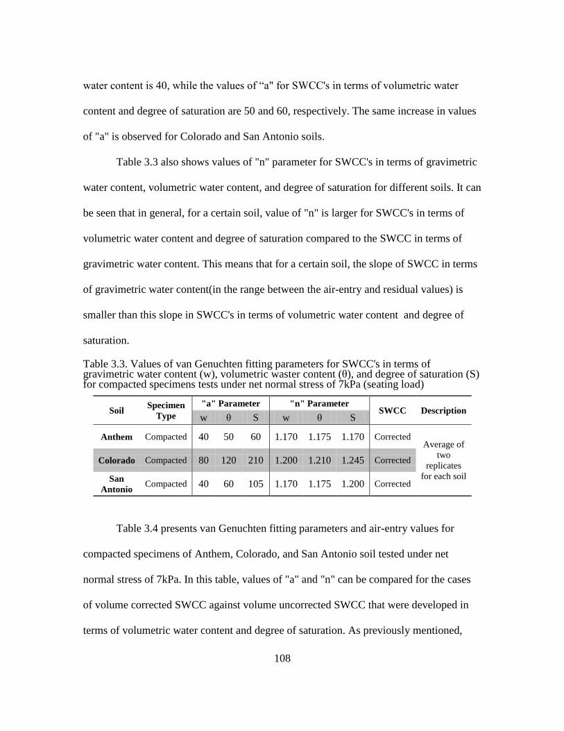
108
water content is 40, while the values of “a" for SWCC's in terms of volumetric water
content and degree of saturation are 50 and 60, respectively. The same increase in values
of "a" is observed for Colorado and San Antonio soils.
Table 3.3 also shows values of "n" parameter for SWCC's in terms of gravimetric
water content, volumetric water content, and degree of saturation for different soils. It can
be seen that in general, for a certain soil, value of "n" is larger for SWCC's in terms of
volumetric water content and degree of saturation compared to the SWCC in terms of
gravimetric water content. This means that for a certain soil, the slope of SWCC in terms
of gravimetric water content(in the range between the air-entry and residual values) is
smaller than this slope in SWCC's in terms of volumetric water content and degree of
saturation.
Table 3.3. Values of van Genuchten fitting parameters for SWCC's in terms of gravimetric water content (w), volumetric waster content (θ), and degree of saturation (S) for compacted specimens tests under net normal stress of 7kPa (seating load)
Soil Specimen
Type
"a" Parameter "n" Parameter SWCC Description
w θ S w θ S
Anthem Compacted 40 50 60 1.170 1.175 1.170 Corrected Average of
two
replicates
for each soil
Colorado Compacted 80 120 210 1.200 1.210 1.245 Corrected
San
Antonio Compacted 40 60 105 1.170 1.175 1.200 Corrected
Table 3.4 presents van Genuchten fitting parameters and air-entry values for
compacted specimens of Anthem, Colorado, and San Antonio soil tested under net
normal stress of 7kPa. In this table, values of "a" and "n" can be compared for the cases
of volume corrected SWCC against volume uncorrected SWCC that were developed in
terms of volumetric water content and degree of saturation. As previously mentioned,
109
volume corrected SWCC's were developed by using the instantaneous volume of the
specimen while in volume uncorrected SWCC's initial volume of the specimen was
utilized and the soil volume change throughout the test was ignored. Data in Table 3.4
demonstrate the difference in the van Genuchten fitting parameters, particularly the "a"
parameter between the volume corrected and uncorrected SWCC. For example, it can be
seen from Table 3.4 that "a" increases from 90 for the volume uncorrected SWCC of
Colorado soil in terms of volumetric water content to 130 for the volume corrected
SWCC. Also "a" increases from 40 for the volume uncorrected SWCC of San Antonio
soil in terms of degree of saturation to 100 for the volume corrected SWCC. Table 3.4
also shows larger AEV for corrected SWCC's compared to uncorrected SWCC's. It can
also be seen that generally AEV is larger for SWCC in terms of degree of saturation
compared to the SWCC in terms of volumetric water content.
The "n" parameter for volume corrected and volume uncorrected SWCC's are also
shown in Table 3.4. It can be seen that for a certain soil, "n" parameter is generally larger
for the volume corrected SWCC (i.e. larger slopes of the curve in the range of air-entry
and residual suctions) compared to the volume uncorrected SWCC. This seems to be the
case for both SWCC's in terms of volumetric water content and degree of saturation.
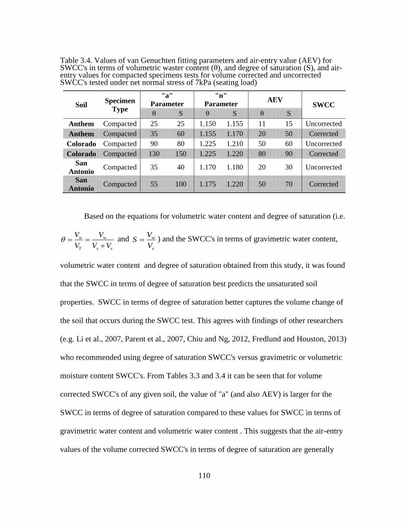
110
Table 3.4. Values of van Genuchten fitting parameters and air-entry value (AEV) for SWCC's in terms of volumetric waster content (θ), and degree of saturation (S), and air-entry values for compacted specimens tests for volume corrected and uncorrected SWCC's tested under net normal stress of 7kPa (seating load)
Soil Specimen
Type
"a"
Parameter
"n"
Parameter AEV
SWCC
θ S θ S θ S
Anthem Compacted 25 25 1.150 1.155 11 15 Uncorrected
Anthem Compacted 35 60 1.155 1.170 20 50 Corrected
Colorado Compacted 90 80 1.225 1.210 50 60 Uncorrected
Colorado Compacted 130 150 1.225 1.220 80 90 Corrected
San
Antonio Compacted 35 40 1.170 1.180 20 30 Uncorrected
San
Antonio Compacted 55 100 1.175 1.220 50 70 Corrected
Based on the equations for volumetric water content and degree of saturation (i.e.
vs
w
T
w
VV
V
V
V
and
v
w
V
VS ) and the SWCC's in terms of gravimetric water content,
volumetric water content and degree of saturation obtained from this study, it was found
that the SWCC in terms of degree of saturation best predicts the unsaturated soil
properties. SWCC in terms of degree of saturation better captures the volume change of
the soil that occurs during the SWCC test. This agrees with findings of other researchers
(e.g. Li et al., 2007, Parent et al., 2007, Chiu and Ng, 2012, Fredlund and Houston, 2013)
who recommended using degree of saturation SWCC's versus gravimetric or volumetric
moisture content SWCC's. From Tables 3.3 and 3.4 it can be seen that for volume
corrected SWCC's of any given soil, the value of "a" (and also AEV) is larger for the
SWCC in terms of degree of saturation compared to these values for SWCC in terms of
gravimetric water content and volumetric water content . This suggests that the air-entry
values of the volume corrected SWCC's in terms of degree of saturation are generally
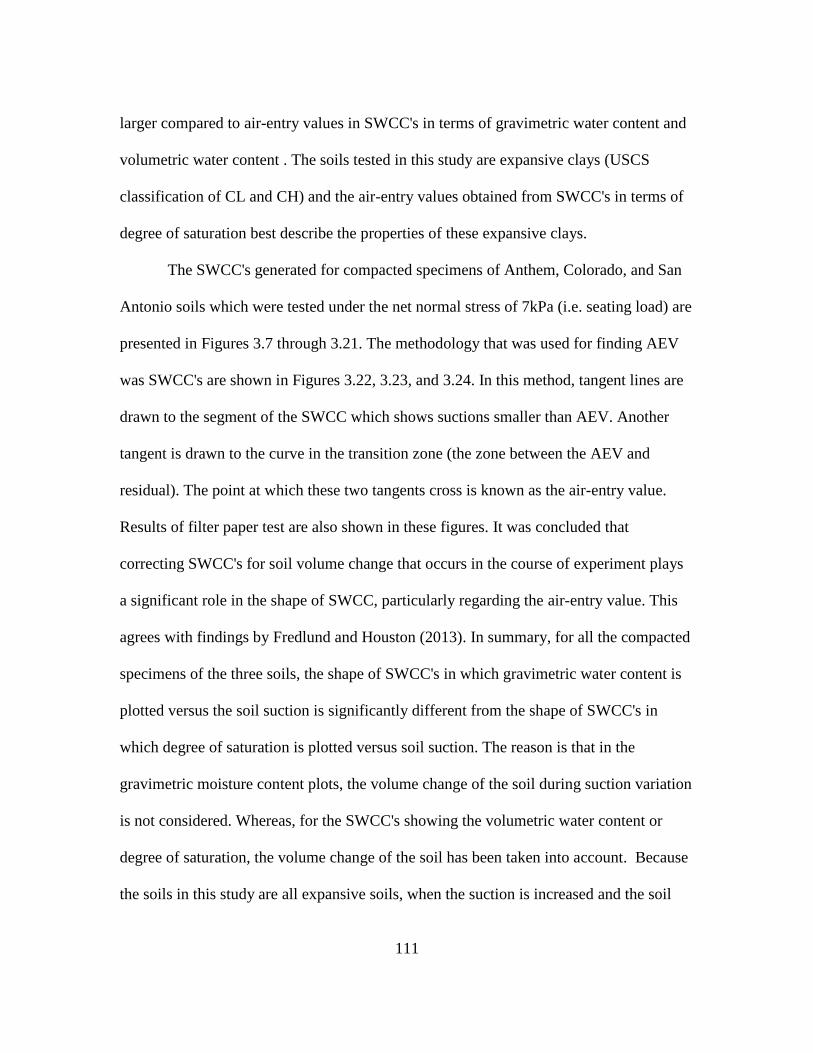
111
larger compared to air-entry values in SWCC's in terms of gravimetric water content and
volumetric water content . The soils tested in this study are expansive clays (USCS
classification of CL and CH) and the air-entry values obtained from SWCC's in terms of
degree of saturation best describe the properties of these expansive clays.
The SWCC's generated for compacted specimens of Anthem, Colorado, and San
Antonio soils which were tested under the net normal stress of 7kPa (i.e. seating load) are
presented in Figures 3.7 through 3.21. The methodology that was used for finding AEV
was SWCC's are shown in Figures 3.22, 3.23, and 3.24. In this method, tangent lines are
drawn to the segment of the SWCC which shows suctions smaller than AEV. Another
tangent is drawn to the curve in the transition zone (the zone between the AEV and
residual). The point at which these two tangents cross is known as the air-entry value.
Results of filter paper test are also shown in these figures. It was concluded that
correcting SWCC's for soil volume change that occurs in the course of experiment plays
a significant role in the shape of SWCC, particularly regarding the air-entry value. This
agrees with findings by Fredlund and Houston (2013). In summary, for all the compacted
specimens of the three soils, the shape of SWCC's in which gravimetric water content is
plotted versus the soil suction is significantly different from the shape of SWCC's in
which degree of saturation is plotted versus soil suction. The reason is that in the
gravimetric moisture content plots, the volume change of the soil during suction variation
is not considered. Whereas, for the SWCC's showing the volumetric water content or
degree of saturation, the volume change of the soil has been taken into account. Because
the soils in this study are all expansive soils, when the suction is increased and the soil
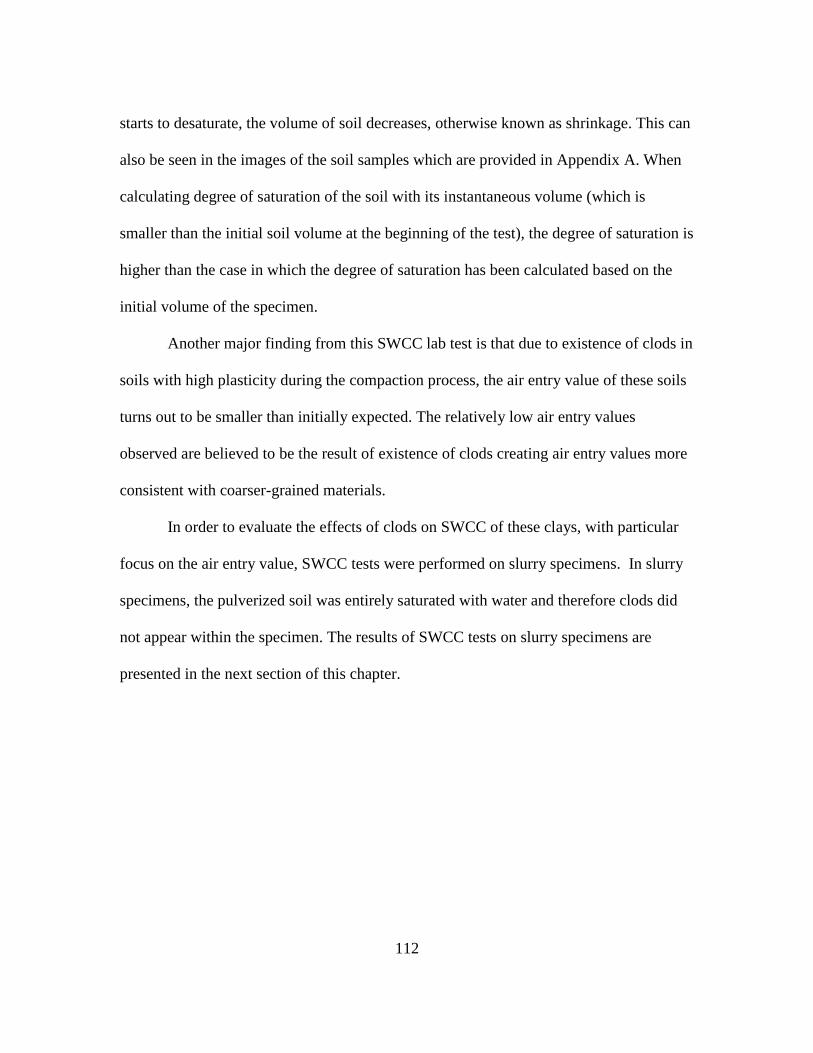
112
starts to desaturate, the volume of soil decreases, otherwise known as shrinkage. This can
also be seen in the images of the soil samples which are provided in Appendix A. When
calculating degree of saturation of the soil with its instantaneous volume (which is
smaller than the initial soil volume at the beginning of the test), the degree of saturation is
higher than the case in which the degree of saturation has been calculated based on the
initial volume of the specimen.
Another major finding from this SWCC lab test is that due to existence of clods in
soils with high plasticity during the compaction process, the air entry value of these soils
turns out to be smaller than initially expected. The relatively low air entry values
observed are believed to be the result of existence of clods creating air entry values more
consistent with coarser-grained materials.
In order to evaluate the effects of clods on SWCC of these clays, with particular
focus on the air entry value, SWCC tests were performed on slurry specimens. In slurry
specimens, the pulverized soil was entirely saturated with water and therefore clods did
not appear within the specimen. The results of SWCC tests on slurry specimens are
presented in the next section of this chapter.
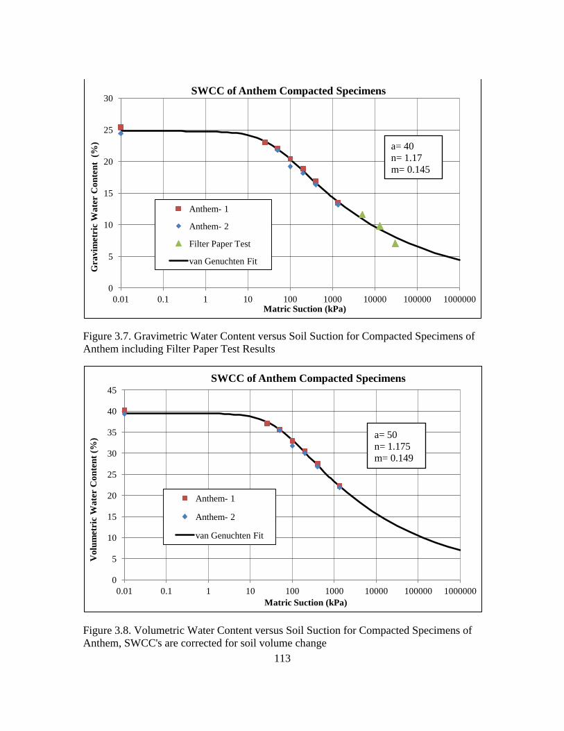
113
Figure 3.7. Gravimetric Water Content versus Soil Suction for Compacted Specimens of
Anthem including Filter Paper Test Results
Figure 3.8. Volumetric Water Content versus Soil Suction for Compacted Specimens of
Anthem, SWCC's are corrected for soil volume change
0
5
10
15
20
25
30
0.01 0.1 1 10 100 1000 10000 100000 1000000
Gra
vim
etri
c W
ate
r C
on
ten
t (
%)
Matric Suction (kPa)
SWCC of Anthem Compacted Specimens
Anthem- 1
Anthem- 2
Filter Paper Test
van Genuchten Fit
a= 40
n= 1.17
m= 0.145
0
5
10
15
20
25
30
35
40
45
0.01 0.1 1 10 100 1000 10000 100000 1000000
Vo
lum
etri
c W
ate
r C
on
ten
t (%
)
Matric Suction (kPa)
SWCC of Anthem Compacted Specimens
Anthem- 1
Anthem- 2
van Genuchten Fit
a= 50
n= 1.175
m= 0.149
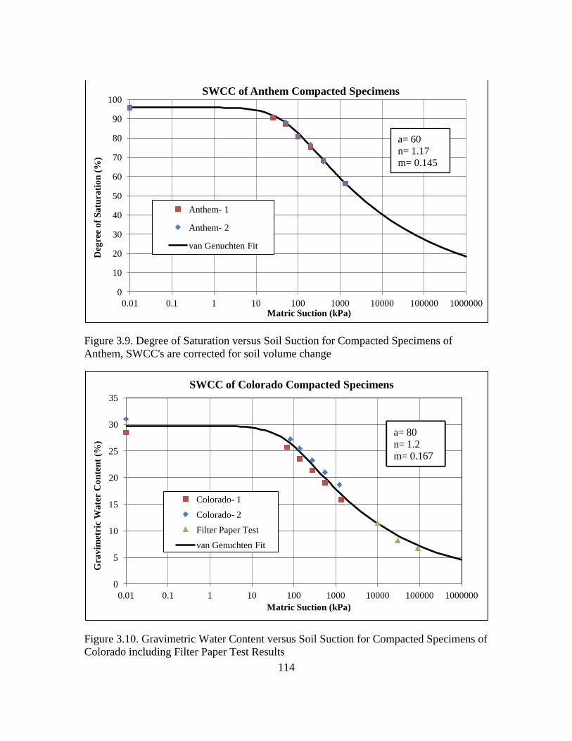
114
Figure 3.9. Degree of Saturation versus Soil Suction for Compacted Specimens of
Anthem, SWCC's are corrected for soil volume change
Figure 3.10. Gravimetric Water Content versus Soil Suction for Compacted Specimens of
Colorado including Filter Paper Test Results
0
10
20
30
40
50
60
70
80
90
100
0.01 0.1 1 10 100 1000 10000 100000 1000000
Deg
ree
of
Sa
tura
tio
n (
%)
Matric Suction (kPa)
SWCC of Anthem Compacted Specimens
Anthem- 1
Anthem- 2
van Genuchten Fit
a= 60
n= 1.17
m= 0.145
0
5
10
15
20
25
30
35
0.01 0.1 1 10 100 1000 10000 100000 1000000
Gra
vim
etri
c W
ate
r C
on
ten
t (%
)
Matric Suction (kPa)
SWCC of Colorado Compacted Specimens
Colorado- 1
Colorado- 2
Filter Paper Test
van Genuchten Fit
a= 40
n= 1.17
m= 0.145
a= 40
n= 1.17
m= 0.145
a= 40
n= 1.17
m= 0.145
a= 40
n= 1.17
m= 0.145
a= 40
n= 1.17
m= 0.145
a= 80
n= 1.2
m= 0.167
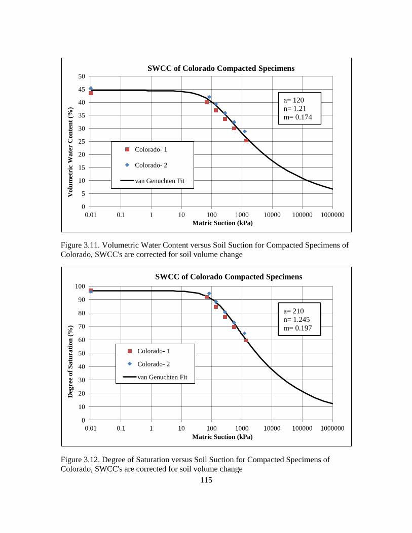
115
Figure 3.11. Volumetric Water Content versus Soil Suction for Compacted Specimens of
Colorado, SWCC's are corrected for soil volume change
Figure 3.12. Degree of Saturation versus Soil Suction for Compacted Specimens of
Colorado, SWCC's are corrected for soil volume change
0
5
10
15
20
25
30
35
40
45
50
0.01 0.1 1 10 100 1000 10000 100000 1000000
Vo
lum
etri
c W
ate
r C
on
ten
t (%
)
Matric Suction (kPa)
SWCC of Colorado Compacted Specimens
Colorado- 1
Colorado- 2
van Genuchten Fit
a= 120
n= 1.21
m= 0.174
0
10
20
30
40
50
60
70
80
90
100
0.01 0.1 1 10 100 1000 10000 100000 1000000
Deg
ree
of
Sa
tura
tio
n (
%)
Matric Suction (kPa)
SWCC of Colorado Compacted Specimens
Colorado- 1
Colorado- 2
van Genuchten Fit
a= 40
n= 1.17
m= 0.145
a= 40
n= 1.17
m= 0.145
a= 40
n= 1.17
m= 0.145
a= 40
n= 1.17
m= 0.145
a= 40
n= 1.17
m= 0.145
a= 85
n= 1.21
m= 0.174
a= 40
n= 1.17
m= 0.145
a= 210
n= 1.245
m= 0.197
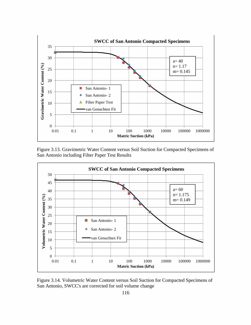
116
Figure 3.13. Gravimetric Water Content versus Soil Suction for Compacted Specimens of
San Antonio including Filter Paper Test Results
Figure 3.14. Volumetric Water Content versus Soil Suction for Compacted Specimens of
San Antonio, SWCC's are corrected for soil volume change
0
5
10
15
20
25
30
35
0.01 0.1 1 10 100 1000 10000 100000 1000000
Gra
vim
etri
c W
ate
r C
on
ten
t (%
)
Matric Suction (kPa)
SWCC of San Antonio Compacted Specimens
San Antonio- 1
San Antonio- 2
Filter Paper Test
van Genuchten Fit
a= 40
n= 1.17
m= 0.145
0
5
10
15
20
25
30
35
40
45
50
0.01 0.1 1 10 100 1000 10000 100000 1000000
Vo
lum
etri
c W
ate
r C
on
ten
t (%
)
Matric Suction (kPa)
SWCC of San Antonio Compacted Specimens
San Antonio- 1
San Antonio- 2
van Genuchten Fit
a= 60
n= 1.175
m= 0.149
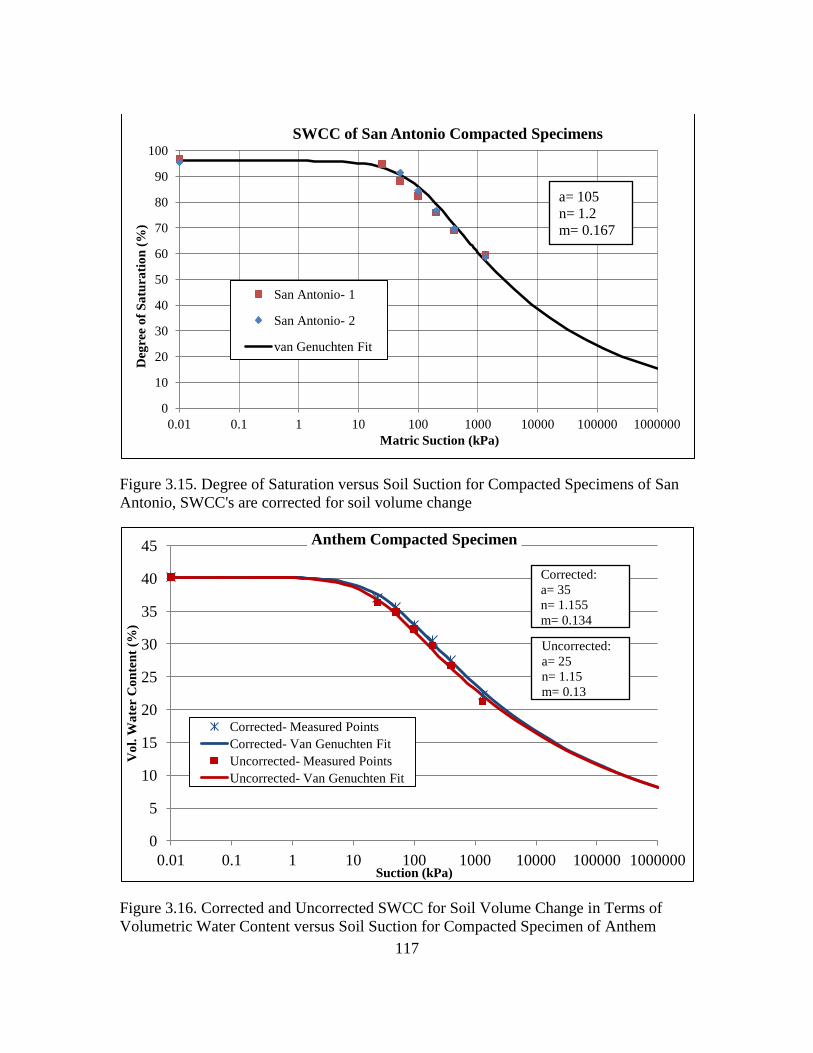
117
Figure 3.15. Degree of Saturation versus Soil Suction for Compacted Specimens of San
Antonio, SWCC's are corrected for soil volume change
Figure 3.16. Corrected and Uncorrected SWCC for Soil Volume Change in Terms of
Volumetric Water Content versus Soil Suction for Compacted Specimen of Anthem
0
10
20
30
40
50
60
70
80
90
100
0.01 0.1 1 10 100 1000 10000 100000 1000000
Deg
ree
of
Sa
tura
tio
n (
%)
Matric Suction (kPa)
SWCC of San Antonio Compacted Specimens
San Antonio- 1
San Antonio- 2
van Genuchten Fit
a= 105
n= 1.2
m= 0.167
0
5
10
15
20
25
30
35
40
45
0.01 0.1 1 10 100 1000 10000 100000 1000000
Vo
l. W
ate
r C
on
ten
t (%
)
Suction (kPa)
Anthem Compacted Specimen
Corrected- Measured Points
Corrected- Van Genuchten Fit
Uncorrected- Measured Points
Uncorrected- Van Genuchten Fit
Corrected:
a= 35
n= 1.155
m= 0.134
Uncorrected:
a= 25
n= 1.15
m= 0.13
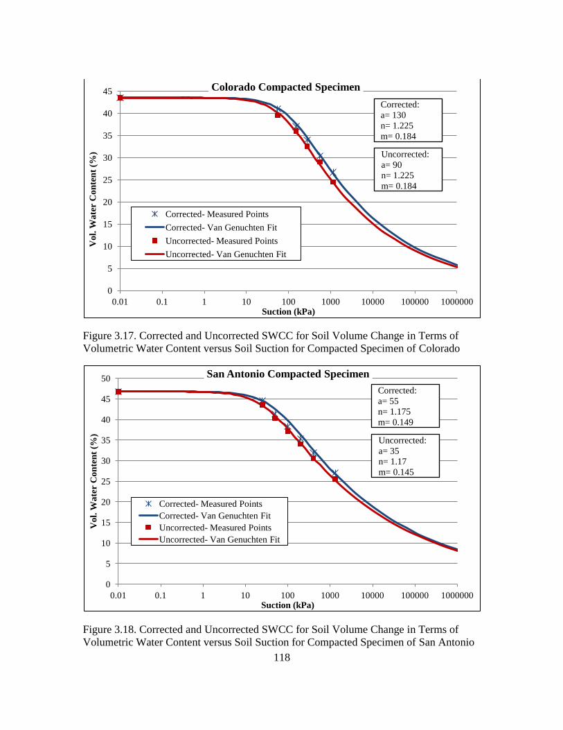
118
Figure 3.17. Corrected and Uncorrected SWCC for Soil Volume Change in Terms of
Volumetric Water Content versus Soil Suction for Compacted Specimen of Colorado
Figure 3.18. Corrected and Uncorrected SWCC for Soil Volume Change in Terms of
Volumetric Water Content versus Soil Suction for Compacted Specimen of San Antonio
0
5
10
15
20
25
30
35
40
45
0.01 0.1 1 10 100 1000 10000 100000 1000000
Vo
l. W
ate
r C
on
ten
t (%
)
Suction (kPa)
Colorado Compacted Specimen
Corrected- Measured Points
Corrected- Van Genuchten Fit
Uncorrected- Measured Points
Uncorrected- Van Genuchten Fit
Corrected:
a= 130
n= 1.225
m= 0.184
Uncorrected:
a= 90
n= 1.225
m= 0.184
0
5
10
15
20
25
30
35
40
45
50
0.01 0.1 1 10 100 1000 10000 100000 1000000
Vo
l. W
ate
r C
on
ten
t (%
)
Suction (kPa)
San Antonio Compacted Specimen
Corrected- Measured Points
Corrected- Van Genuchten Fit
Uncorrected- Measured Points
Uncorrected- Van Genuchten Fit
Corrected:
a= 55
n= 1.175
m= 0.149
Uncorrected:
a= 35
n= 1.17
m= 0.145
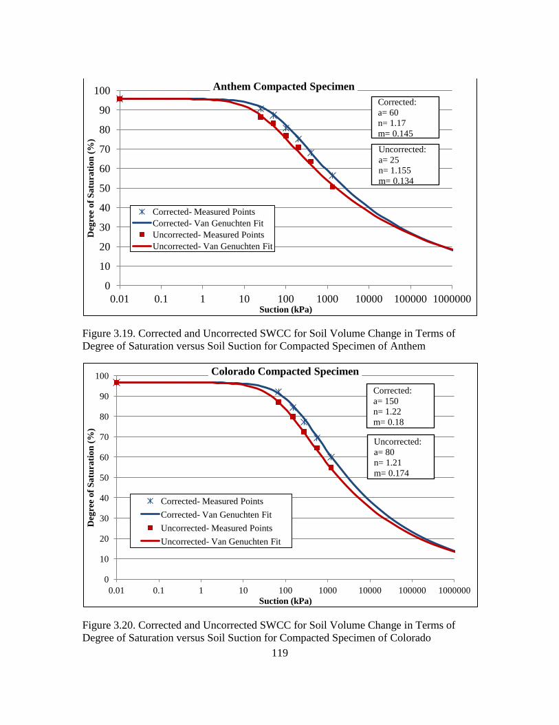
119
Figure 3.19. Corrected and Uncorrected SWCC for Soil Volume Change in Terms of
Degree of Saturation versus Soil Suction for Compacted Specimen of Anthem
Figure 3.20. Corrected and Uncorrected SWCC for Soil Volume Change in Terms of
Degree of Saturation versus Soil Suction for Compacted Specimen of Colorado
0
10
20
30
40
50
60
70
80
90
100
0.01 0.1 1 10 100 1000 10000 100000 1000000
Deg
ree
of
Sa
tura
tio
n (
%)
Suction (kPa)
Anthem Compacted Specimen
Corrected- Measured Points
Corrected- Van Genuchten Fit
Uncorrected- Measured Points
Uncorrected- Van Genuchten Fit
Corrected:
a= 60
n= 1.17
m= 0.145
Uncorrected:
a= 25
n= 1.155
m= 0.134
0
10
20
30
40
50
60
70
80
90
100
0.01 0.1 1 10 100 1000 10000 100000 1000000
Deg
ree
of
Sa
tura
tio
n (
%)
Suction (kPa)
Colorado Compacted Specimen
Corrected- Measured Points
Corrected- Van Genuchten Fit
Uncorrected- Measured Points
Uncorrected- Van Genuchten Fit
Corrected:
a= 150
n= 1.22
m= 0.18
Uncorrected:
a= 80
n= 1.21
m= 0.174
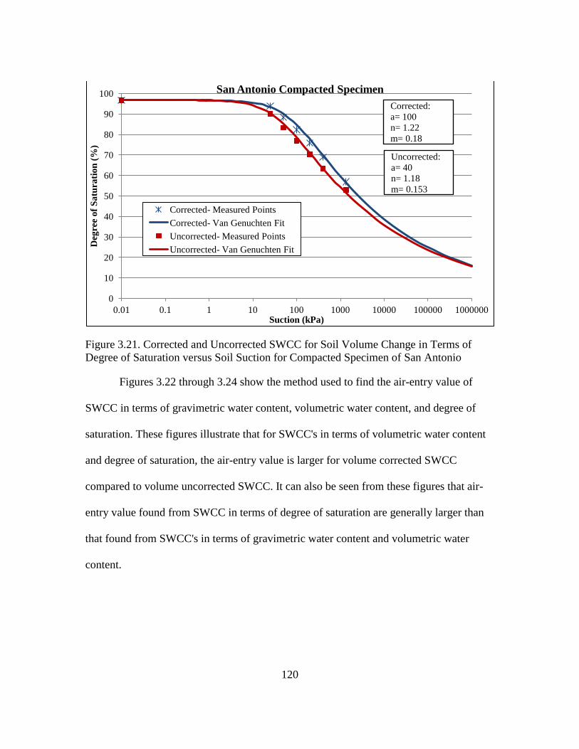
120
Figure 3.21. Corrected and Uncorrected SWCC for Soil Volume Change in Terms of
Degree of Saturation versus Soil Suction for Compacted Specimen of San Antonio
Figures 3.22 through 3.24 show the method used to find the air-entry value of
SWCC in terms of gravimetric water content, volumetric water content, and degree of
saturation. These figures illustrate that for SWCC's in terms of volumetric water content
and degree of saturation, the air-entry value is larger for volume corrected SWCC
compared to volume uncorrected SWCC. It can also be seen from these figures that air-
entry value found from SWCC in terms of degree of saturation are generally larger than
that found from SWCC's in terms of gravimetric water content and volumetric water
content.
0
10
20
30
40
50
60
70
80
90
100
0.01 0.1 1 10 100 1000 10000 100000 1000000
Deg
ree
of
Sa
tura
tio
n (
%)
Suction (kPa)
San Antonio Compacted Specimen
Corrected- Measured Points
Corrected- Van Genuchten Fit
Uncorrected- Measured Points
Uncorrected- Van Genuchten Fit
Corrected:
a= 100
n= 1.22
m= 0.18
Uncorrected:
a= 40
n= 1.18
m= 0.153
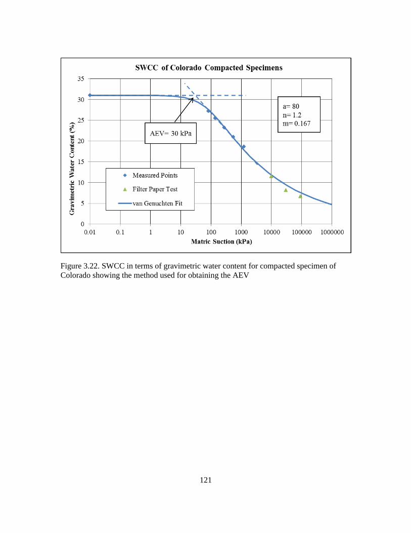
121
Figure 3.22. SWCC in terms of gravimetric water content for compacted specimen of
Colorado showing the method used for obtaining the AEV
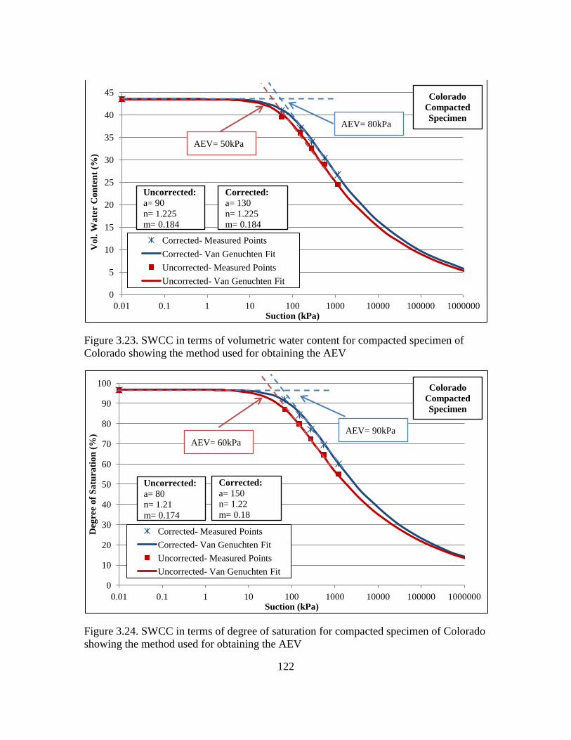
122
Figure 3.23. SWCC in terms of volumetric water content for compacted specimen of
Colorado showing the method used for obtaining the AEV
Figure 3.24. SWCC in terms of degree of saturation for compacted specimen of Colorado
showing the method used for obtaining the AEV
0
5
10
15
20
25
30
35
40
45
0.01 0.1 1 10 100 1000 10000 100000 1000000
Vo
l. W
ate
r C
on
ten
t (%
)
Suction (kPa)
Corrected- Measured Points
Corrected- Van Genuchten Fit
Uncorrected- Measured Points
Uncorrected- Van Genuchten Fit
Corrected:
a= 130
n= 1.225
m= 0.184
Uncorrected:
a= 90
n= 1.225
m= 0.184
AEV= 80kPa
AEV= 50kPa
Colorado
Compacted
Specimen
0
10
20
30
40
50
60
70
80
90
100
0.01 0.1 1 10 100 1000 10000 100000 1000000
Deg
ree
of
Sa
tura
tio
n (
%)
Suction (kPa)
Corrected- Measured Points
Corrected- Van Genuchten Fit
Uncorrected- Measured Points
Uncorrected- Van Genuchten Fit
Corrected:
a= 150
n= 1.22
m= 0.18
Uncorrected:
a= 80
n= 1.21
m= 0.174
AEV= 90kPa
AEV= 60kPa
Colorado
Compacted
Specimen
123
3.5.2. SWCC of Slurry Specimens
The slurry specimens were prepared by mixing certain amount of soil and water
to make sure that the specimen had reached 100% saturation. Drying SWCC test was
then conducted on saturated specimens (of three soil types of Anthem, Colorado, and San
Antonio). Moisture content and volume change of the specimens were measured during
the test and SWCC's were established for these slurry specimens. SWCC's in terms of
volumetric moisture content and degree of saturation were corrected for soil volume
change during the test. These SWCC's are shown in Figures 3.25 through 3.33.
It should be mentioned that performing SWCC on slurry specimens in the 1-D
device is rather challenging due to very high and often non-uniform volume change of
these specimens, which often present challenges regarding measuring the volume change
if the specimen during changes in matric suction. It is recommended that image
processing software be utilized for measurement of volume change of slurry specimens.
The difficulty in volume change measurement of slurry specimens was
pronounced for low net normal stresses. It was found that applying net normal stresses to
the slurry specimens (even small net normal stresses in the order of 3- 7kPa) leads to
more uniform shrinkage of the specimens. Uniform volume changes are generally easier
to measure. Therefore, in all of the SWCC tests on slurry specimens a token load of 3kPa
was used. Another advantage of using a token load is to ensure a good contact between
the specimen and the high air-entry disc of the SWCC device throughout the test.
As for compacted specimens, it was found that for slurry specimens too,
correcting SWCC's for soil volume change plays a significant role in shape of the SWCC
124
and particularly on the air-entry value. This was found by comparing SWCC's in terms of
gravimetric moisture content versus SWCC's in terms of degree of saturation and
volumetric moisture content. SWCC's in terms of gravimetric moisture content are not
corrected for soil volume change (as they are generated based on masses of water and dry
soil), while SWCC's in terms of degree of saturation and volumetric moisture content
were corrected for volume change. Large differences were found between shapes of
SWCC's corrected and uncorrected for volume change that were established for slurry
specimens. Since the volume change of slurry specimens are significantly larger than the
volume change of compacted specimens, the difference between the volume corrected
and uncorrected SWCC's were found to be significantly larger for slurry specimens
compared to compacted specimens. This is shown in Figures 3.27, 3.30, and 3.33 which
present SWCC's in terms of degree of saturation established for slurry specimens.
It was found that SWCC's corrected for volume change (particularly SWCC in
terms of degree of saturation) are the better indicator of true air entry value of soils which
undergo significant volume change during suction variation (such as slurry specimens).
Table 3.5 presents values of "a" and "n" parameters of the van Genuchten fit for
establishing SWCC's of slurry specimens in terms of gravimetric water content,
volumetric water content, and degree of saturation.
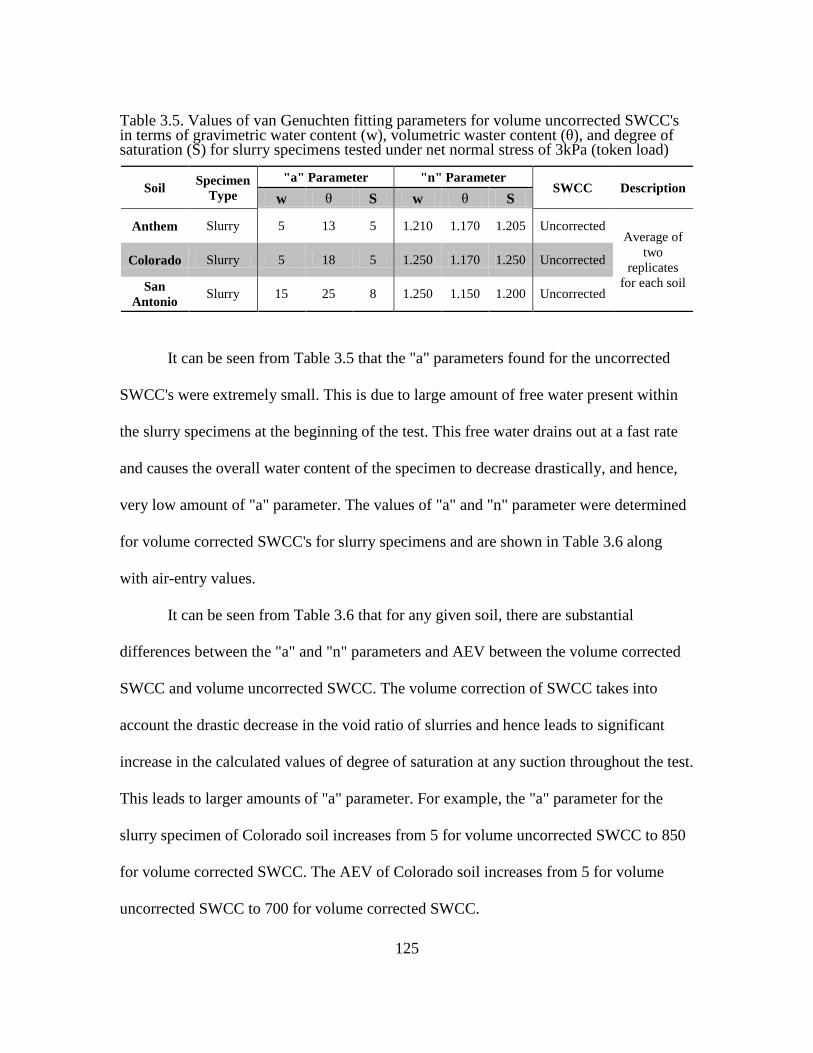
125
Table 3.5. Values of van Genuchten fitting parameters for volume uncorrected SWCC's in terms of gravimetric water content (w), volumetric waster content (θ), and degree of saturation (S) for slurry specimens tested under net normal stress of 3kPa (token load)
Soil Specimen
Type
"a" Parameter "n" Parameter SWCC Description
w θ S w θ S
Anthem Slurry 5 13 5 1.210 1.170 1.205 Uncorrected Average of
two
replicates
for each soil
Colorado Slurry 5 18 5 1.250 1.170 1.250 Uncorrected
San
Antonio Slurry 15 25 8 1.250 1.150 1.200 Uncorrected
It can be seen from Table 3.5 that the "a" parameters found for the uncorrected
SWCC's were extremely small. This is due to large amount of free water present within
the slurry specimens at the beginning of the test. This free water drains out at a fast rate
and causes the overall water content of the specimen to decrease drastically, and hence,
very low amount of "a" parameter. The values of "a" and "n" parameter were determined
for volume corrected SWCC's for slurry specimens and are shown in Table 3.6 along
with air-entry values.
It can be seen from Table 3.6 that for any given soil, there are substantial
differences between the "a" and "n" parameters and AEV between the volume corrected
SWCC and volume uncorrected SWCC. The volume correction of SWCC takes into
account the drastic decrease in the void ratio of slurries and hence leads to significant
increase in the calculated values of degree of saturation at any suction throughout the test.
This leads to larger amounts of "a" parameter. For example, the "a" parameter for the
slurry specimen of Colorado soil increases from 5 for volume uncorrected SWCC to 850
for volume corrected SWCC. The AEV of Colorado soil increases from 5 for volume
uncorrected SWCC to 700 for volume corrected SWCC.
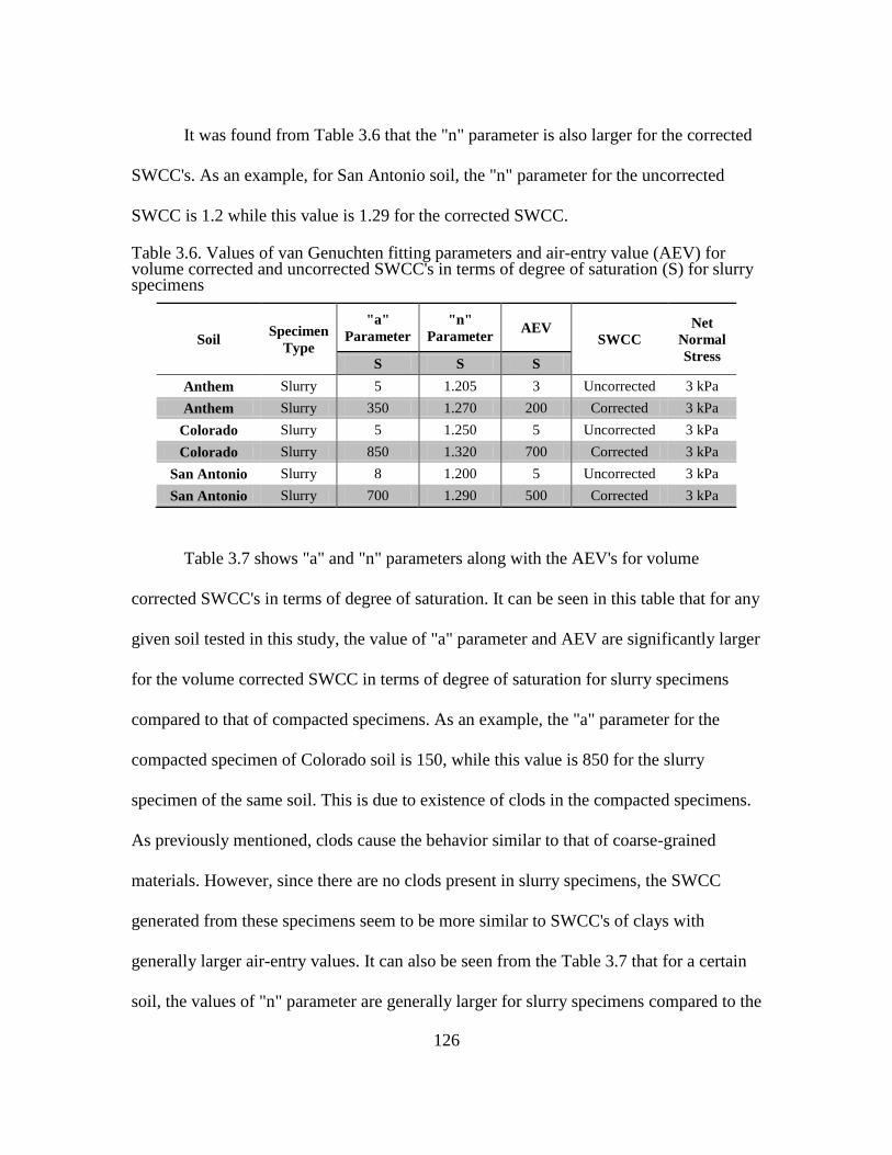
126
It was found from Table 3.6 that the "n" parameter is also larger for the corrected
SWCC's. As an example, for San Antonio soil, the "n" parameter for the uncorrected
SWCC is 1.2 while this value is 1.29 for the corrected SWCC.
Table 3.6. Values of van Genuchten fitting parameters and air-entry value (AEV) for volume corrected and uncorrected SWCC's in terms of degree of saturation (S) for slurry specimens
Soil Specimen
Type
"a"
Parameter
"n"
Parameter AEV
SWCC
Net
Normal
Stress S S S
Anthem Slurry 5 1.205 3 Uncorrected 3 kPa
Anthem Slurry 350 1.270 200 Corrected 3 kPa
Colorado Slurry 5 1.250 5 Uncorrected 3 kPa
Colorado Slurry 850 1.320 700 Corrected 3 kPa
San Antonio Slurry 8 1.200 5 Uncorrected 3 kPa
San Antonio Slurry 700 1.290 500 Corrected 3 kPa
Table 3.7 shows "a" and "n" parameters along with the AEV's for volume
corrected SWCC's in terms of degree of saturation. It can be seen in this table that for any
given soil tested in this study, the value of "a" parameter and AEV are significantly larger
for the volume corrected SWCC in terms of degree of saturation for slurry specimens
compared to that of compacted specimens. As an example, the "a" parameter for the
compacted specimen of Colorado soil is 150, while this value is 850 for the slurry
specimen of the same soil. This is due to existence of clods in the compacted specimens.
As previously mentioned, clods cause the behavior similar to that of coarse-grained
materials. However, since there are no clods present in slurry specimens, the SWCC
generated from these specimens seem to be more similar to SWCC's of clays with
generally larger air-entry values. It can also be seen from the Table 3.7 that for a certain
soil, the values of "n" parameter are generally larger for slurry specimens compared to the
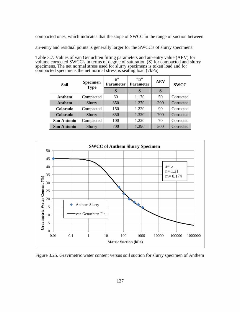
127
compacted ones, which indicates that the slope of SWCC in the range of suction between
air-entry and residual points is generally larger for the SWCC's of slurry specimens.
Table 3.7. Values of van Genuchten fitting parameters and air-entry value (AEV) for volume corrected SWCC's in terms of degree of saturation (S) for compacted and slurry specimens. The net normal stress used for slurry specimens is token load and for compacted specimens the net normal stress is seating load (7kPa)
Soil Specimen
Type
"a"
Parameter
"n"
Parameter AEV
SWCC
S S S
Anthem Compacted 60 1.170 50 Corrected
Anthem Slurry 350 1.270 200 Corrected
Colorado Compacted 150 1.220 90 Corrected
Colorado Slurry 850 1.320 700 Corrected
San Antonio Compacted 100 1.220 70 Corrected
San Antonio Slurry 700 1.290 500 Corrected
Figure 3.25. Gravimetric water content versus soil suction for slurry specimen of Anthem
0
5
10
15
20
25
30
35
40
45
50
0.01 0.1 1 10 100 1000 10000 100000 1000000
Gra
vim
etri
c W
ate
r C
on
ten
t (%
)
Matric Suction (kPa)
SWCC of Anthem Slurry Specimen
Anthem Slurry
van Genuchten Fit
a= 5
n= 1.21
m= 0.174
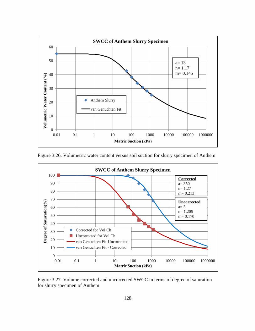
128
Figure 3.26. Volumetric water content versus soil suction for slurry specimen of Anthem
Figure 3.27. Volume corrected and uncorrected SWCC in terms of degree of saturation
for slurry specimen of Anthem
0
10
20
30
40
50
60
0.01 0.1 1 10 100 1000 10000 100000 1000000
Vo
lum
etri
c W
ate
r C
on
ten
t (%
)
Matric Suction (kPa)
SWCC of Anthem Slurry Specimen
Anthem Slurry
van Genuchten Fit
a= 13
n= 1.17
m= 0.145
0
10
20
30
40
50
60
70
80
90
100
0.01 0.1 1 10 100 1000 10000 100000 1000000
Deg
ree
of
Sa
tura
tio
n(%
)
Matric Suction (kPa)
SWCC of Anthem Slurry Specimen
Corrected for Vol Ch
Uncorrected for Vol Ch
van Genuchten Fit-Uncorrected
van Genuchten Fit - Corrected
Uncorrected
a= 5
n= 1.205
m= 0.170
Corrected
a= 350
n= 1.27
m= 0.213
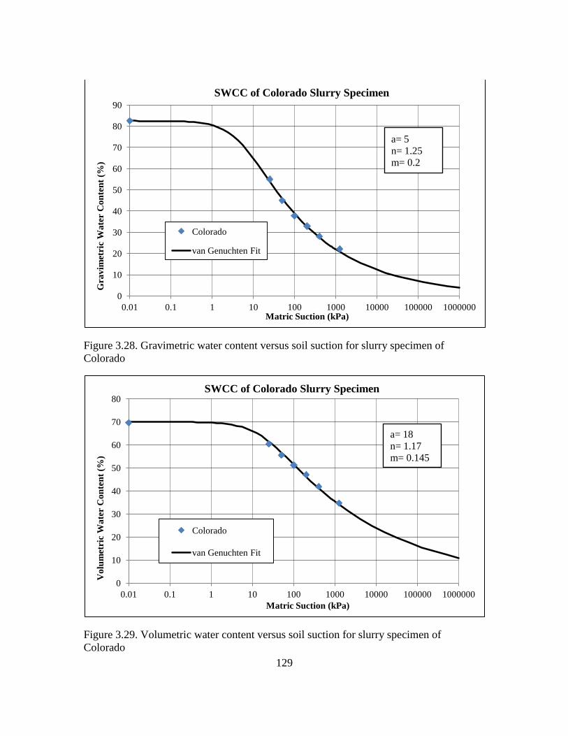
129
Figure 3.28. Gravimetric water content versus soil suction for slurry specimen of
Colorado
Figure 3.29. Volumetric water content versus soil suction for slurry specimen of
Colorado
0
10
20
30
40
50
60
70
80
90
0.01 0.1 1 10 100 1000 10000 100000 1000000
Gra
vim
etri
c W
ate
r C
on
ten
t (%
)
Matric Suction (kPa)
SWCC of Colorado Slurry Specimen
Colorado
van Genuchten Fit
a= 5
n= 1.25
m= 0.2
0
10
20
30
40
50
60
70
80
0.01 0.1 1 10 100 1000 10000 100000 1000000
Vo
lum
etri
c W
ate
r C
on
ten
t (%
)
Matric Suction (kPa)
SWCC of Colorado Slurry Specimen
Colorado
van Genuchten Fit
a= 18
n= 1.17
m= 0.145
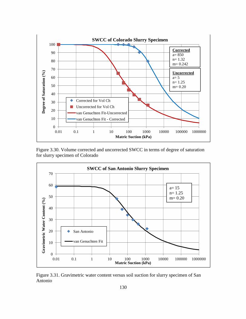
130
Figure 3.30. Volume corrected and uncorrected SWCC in terms of degree of saturation
for slurry specimen of Colorado
Figure 3.31. Gravimetric water content versus soil suction for slurry specimen of San
Antonio
0
10
20
30
40
50
60
70
80
90
100
0.01 0.1 1 10 100 1000 10000 100000 1000000
Deg
ree
of
Sa
tura
tio
n (
%)
Matric Suction (kPa)
SWCC of Colorado Slurry Specimen
Corrected for Vol Ch
Uncorrected for Vol Ch
van Genuchten Fit-Uncorrected
van Genuchten Fit - Corrected
Uncorrected
a= 5
n= 1.25
m= 0.20
Corrected
a= 850
n= 1.32
m= 0.242
0
10
20
30
40
50
60
70
0.01 0.1 1 10 100 1000 10000 100000 1000000
Gra
vim
etri
c W
ate
r C
on
ten
t (%
)
Matric Suction (kPa)
SWCC of San Antonio Slurry Specimen
San Antonio
van Genuchten Fit
a= 15
n= 1.25
m= 0.20
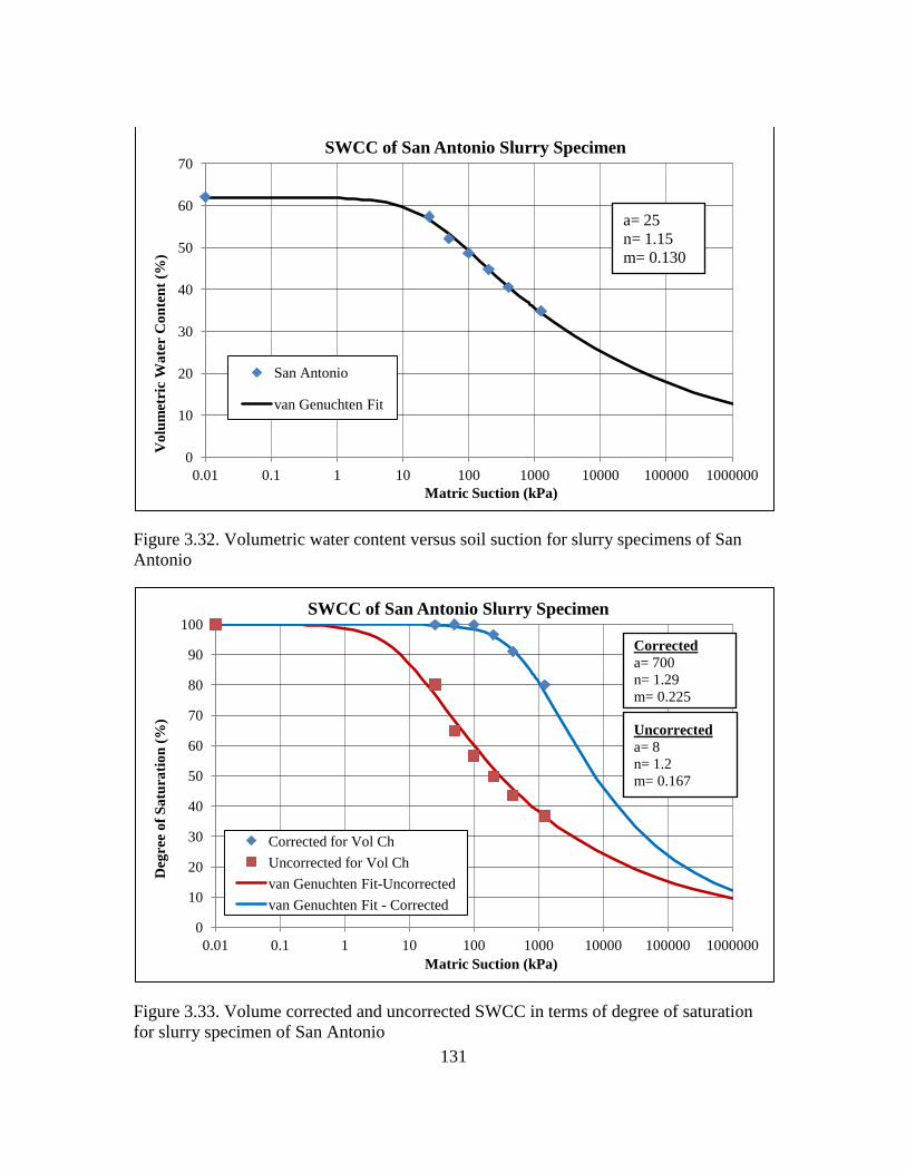
131
Figure 3.32. Volumetric water content versus soil suction for slurry specimens of San
Antonio
Figure 3.33. Volume corrected and uncorrected SWCC in terms of degree of saturation
for slurry specimen of San Antonio
0
10
20
30
40
50
60
70
0.01 0.1 1 10 100 1000 10000 100000 1000000
Vo
lum
etri
c W
ate
r C
on
ten
t (%
)
Matric Suction (kPa)
SWCC of San Antonio Slurry Specimen
San Antonio
van Genuchten Fit
a= 25
n= 1.15
m= 0.130
0
10
20
30
40
50
60
70
80
90
100
0.01 0.1 1 10 100 1000 10000 100000 1000000
Deg
ree
of
Sa
tura
tio
n (
%)
Matric Suction (kPa)
SWCC of San Antonio Slurry Specimen
Corrected for Vol Ch
Uncorrected for Vol Ch
van Genuchten Fit-Uncorrected
van Genuchten Fit - Corrected
Uncorrected
a= 8
n= 1.2
m= 0.167
Corrected
a= 700
n= 1.29
m= 0.225
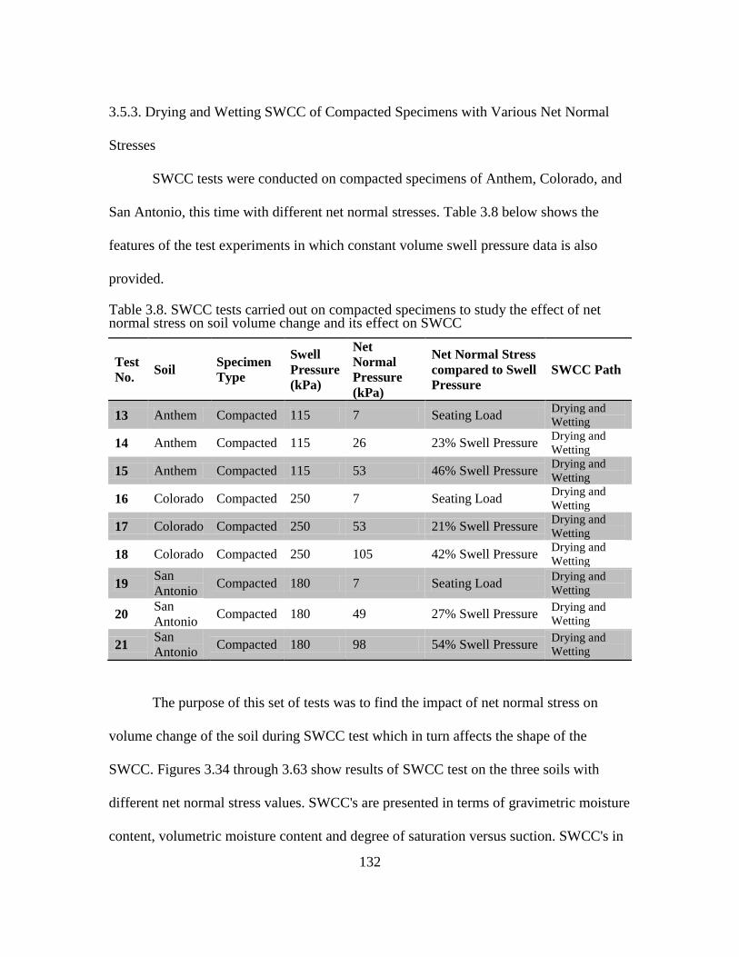
132
3.5.3. Drying and Wetting SWCC of Compacted Specimens with Various Net Normal
Stresses
SWCC tests were conducted on compacted specimens of Anthem, Colorado, and
San Antonio, this time with different net normal stresses. Table 3.8 below shows the
features of the test experiments in which constant volume swell pressure data is also
provided.
Table 3.8. SWCC tests carried out on compacted specimens to study the effect of net normal stress on soil volume change and its effect on SWCC
Test
No. Soil
Specimen
Type
Swell
Pressure
(kPa)
Net
Normal
Pressure
(kPa)
Net Normal Stress
compared to Swell
Pressure
SWCC Path
13 Anthem Compacted 115 7 Seating Load Drying and
Wetting
14 Anthem Compacted 115 26 23% Swell Pressure Drying and
Wetting
15 Anthem Compacted 115 53 46% Swell Pressure Drying and
Wetting
16 Colorado Compacted 250 7 Seating Load Drying and
Wetting
17 Colorado Compacted 250 53 21% Swell Pressure Drying and
Wetting
18 Colorado Compacted 250 105 42% Swell Pressure Drying and
Wetting
19 San
Antonio Compacted 180 7 Seating Load
Drying and
Wetting
20 San
Antonio Compacted 180 49 27% Swell Pressure
Drying and
Wetting
21 San
Antonio Compacted 180 98 54% Swell Pressure
Drying and
Wetting
The purpose of this set of tests was to find the impact of net normal stress on
volume change of the soil during SWCC test which in turn affects the shape of the
SWCC. Figures 3.34 through 3.63 show results of SWCC test on the three soils with
different net normal stress values. SWCC's are presented in terms of gravimetric moisture
content, volumetric moisture content and degree of saturation versus suction. SWCC's in
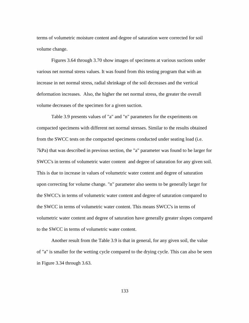
133
terms of volumetric moisture content and degree of saturation were corrected for soil
volume change.
Figures 3.64 through 3.70 show images of specimens at various suctions under
various net normal stress values. It was found from this testing program that with an
increase in net normal stress, radial shrinkage of the soil decreases and the vertical
deformation increases. Also, the higher the net normal stress, the greater the overall
volume decreases of the specimen for a given suction.
Table 3.9 presents values of "a" and "n" parameters for the experiments on
compacted specimens with different net normal stresses. Similar to the results obtained
from the SWCC tests on the compacted specimens conducted under seating load (i.e.
7kPa) that was described in previous section, the "a" parameter was found to be larger for
SWCC's in terms of volumetric water content and degree of saturation for any given soil.
This is due to increase in values of volumetric water content and degree of saturation
upon correcting for volume change. "n" parameter also seems to be generally larger for
the SWCC's in terms of volumetric water content and degree of saturation compared to
the SWCC in terms of volumetric water content. This means SWCC's in terms of
volumetric water content and degree of saturation have generally greater slopes compared
to the SWCC in terms of volumetric water content.
Another result from the Table 3.9 is that in general, for any given soil, the value
of "a" is smaller for the wetting cycle compared to the drying cycle. This can also be seen
in Figure 3.34 through 3.63.
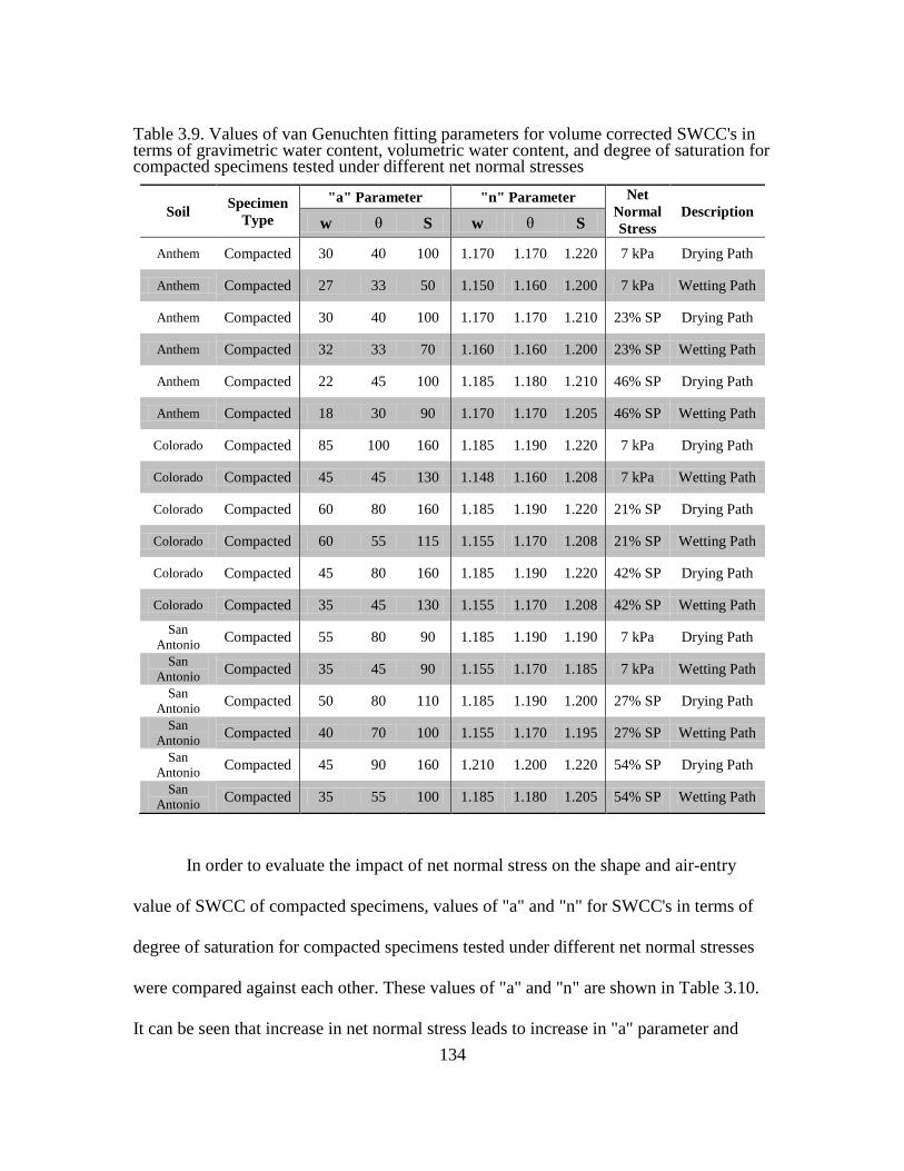
134
Table 3.9. Values of van Genuchten fitting parameters for volume corrected SWCC's in terms of gravimetric water content, volumetric water content, and degree of saturation for compacted specimens tested under different net normal stresses
Soil Specimen
Type
"a" Parameter "n" Parameter Net
Normal
Stress
Description w θ S w θ S
Anthem Compacted 30 40 100 1.170 1.170 1.220 7 kPa Drying Path
Anthem Compacted 27 33 50 1.150 1.160 1.200 7 kPa Wetting Path
Anthem Compacted 30 40 100 1.170 1.170 1.210 23% SP Drying Path
Anthem Compacted 32 33 70 1.160 1.160 1.200 23% SP Wetting Path
Anthem Compacted 22 45 100 1.185 1.180 1.210 46% SP Drying Path
Anthem Compacted 18 30 90 1.170 1.170 1.205 46% SP Wetting Path
Colorado Compacted 85 100 160 1.185 1.190 1.220 7 kPa Drying Path
Colorado Compacted 45 45 130 1.148 1.160 1.208 7 kPa Wetting Path
Colorado Compacted 60 80 160 1.185 1.190 1.220 21% SP Drying Path
Colorado Compacted 60 55 115 1.155 1.170 1.208 21% SP Wetting Path
Colorado Compacted 45 80 160 1.185 1.190 1.220 42% SP Drying Path
Colorado Compacted 35 45 130 1.155 1.170 1.208 42% SP Wetting Path
San
Antonio Compacted 55 80 90 1.185 1.190 1.190 7 kPa Drying Path
San
Antonio Compacted 35 45 90 1.155 1.170 1.185 7 kPa Wetting Path
San
Antonio Compacted 50 80 110 1.185 1.190 1.200 27% SP Drying Path
San
Antonio Compacted 40 70 100 1.155 1.170 1.195 27% SP Wetting Path
San
Antonio Compacted 45 90 160 1.210 1.200 1.220 54% SP Drying Path
San
Antonio Compacted 35 55 100 1.185 1.180 1.205 54% SP Wetting Path
In order to evaluate the impact of net normal stress on the shape and air-entry
value of SWCC of compacted specimens, values of "a" and "n" for SWCC's in terms of
degree of saturation for compacted specimens tested under different net normal stresses
were compared against each other. These values of "a" and "n" are shown in Table 3.10.
It can be seen that increase in net normal stress leads to increase in "a" parameter and
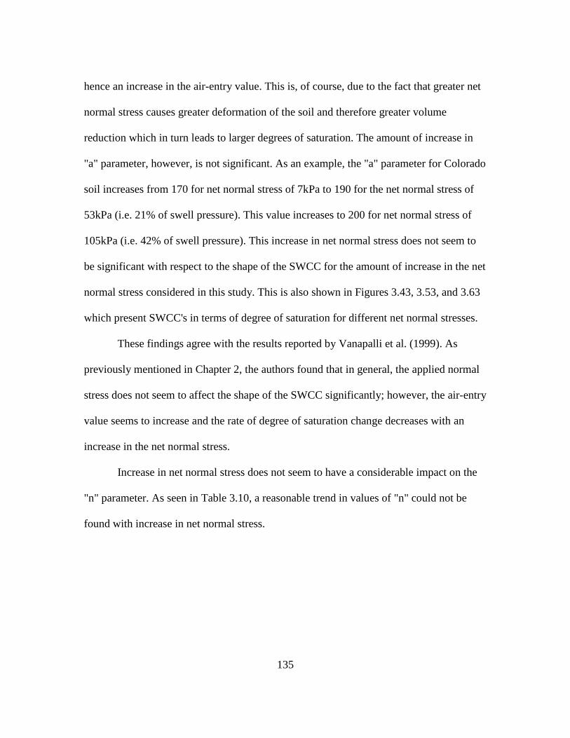
135
hence an increase in the air-entry value. This is, of course, due to the fact that greater net
normal stress causes greater deformation of the soil and therefore greater volume
reduction which in turn leads to larger degrees of saturation. The amount of increase in
"a" parameter, however, is not significant. As an example, the "a" parameter for Colorado
soil increases from 170 for net normal stress of 7kPa to 190 for the net normal stress of
53kPa (i.e. 21% of swell pressure). This value increases to 200 for net normal stress of
105kPa (i.e. 42% of swell pressure). This increase in net normal stress does not seem to
be significant with respect to the shape of the SWCC for the amount of increase in the net
normal stress considered in this study. This is also shown in Figures 3.43, 3.53, and 3.63
which present SWCC's in terms of degree of saturation for different net normal stresses.
These findings agree with the results reported by Vanapalli et al. (1999). As
previously mentioned in Chapter 2, the authors found that in general, the applied normal
stress does not seem to affect the shape of the SWCC significantly; however, the air-entry
value seems to increase and the rate of degree of saturation change decreases with an
increase in the net normal stress.
Increase in net normal stress does not seem to have a considerable impact on the
"n" parameter. As seen in Table 3.10, a reasonable trend in values of "n" could not be
found with increase in net normal stress.
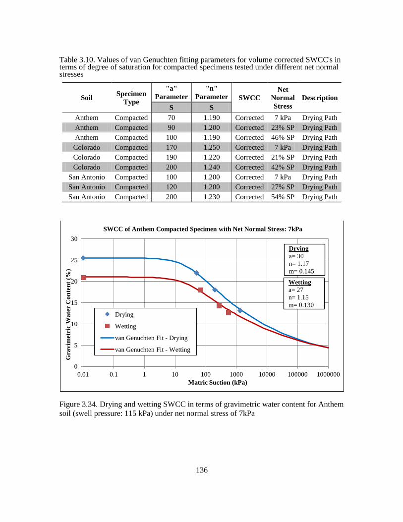
136
Table 3.10. Values of van Genuchten fitting parameters for volume corrected SWCC's in terms of degree of saturation for compacted specimens tested under different net normal stresses
Soil Specimen
Type
"a"
Parameter
"n"
Parameter SWCC
Net
Normal
Stress
Description
S S
Anthem Compacted 70 1.190 Corrected 7 kPa Drying Path
Anthem Compacted 90 1.200 Corrected 23% SP Drying Path
Anthem Compacted 100 1.190 Corrected 46% SP Drying Path
Colorado Compacted 170 1.250 Corrected 7 kPa Drying Path
Colorado Compacted 190 1.220 Corrected 21% SP Drying Path
Colorado Compacted 200 1.240 Corrected 42% SP Drying Path
San Antonio Compacted 100 1.200 Corrected 7 kPa Drying Path
San Antonio Compacted 120 1.200 Corrected 27% SP Drying Path
San Antonio Compacted 200 1.230 Corrected 54% SP Drying Path
Figure 3.34. Drying and wetting SWCC in terms of gravimetric water content for Anthem
soil (swell pressure: 115 kPa) under net normal stress of 7kPa
0
5
10
15
20
25
30
0.01 0.1 1 10 100 1000 10000 100000 1000000
Gra
vim
etri
c W
ate
r C
on
ten
t (%
)
Matric Suction (kPa)
SWCC of Anthem Compacted Specimen with Net Normal Stress: 7kPa
Drying
Wetting
van Genuchten Fit - Drying
van Genuchten Fit - Wetting
Drying
a= 30
n= 1.17
m= 0.145
Wetting
a= 27
n= 1.15
m= 0.130
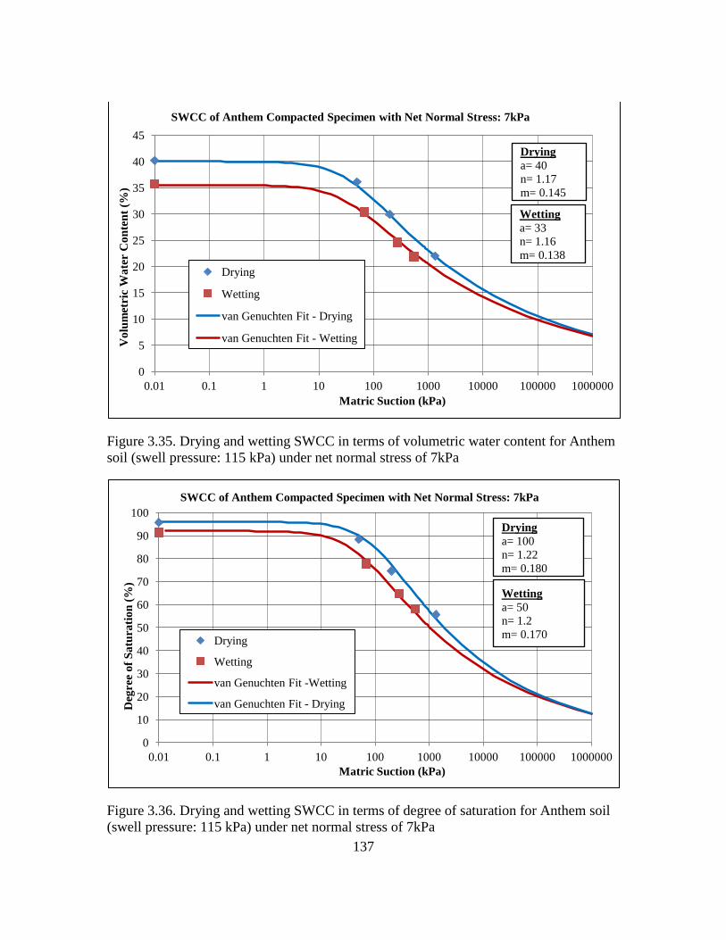
137
Figure 3.35. Drying and wetting SWCC in terms of volumetric water content for Anthem
soil (swell pressure: 115 kPa) under net normal stress of 7kPa
Figure 3.36. Drying and wetting SWCC in terms of degree of saturation for Anthem soil
(swell pressure: 115 kPa) under net normal stress of 7kPa
0
5
10
15
20
25
30
35
40
45
0.01 0.1 1 10 100 1000 10000 100000 1000000
Vo
lum
etri
c W
ate
r C
on
ten
t (%
)
Matric Suction (kPa)
SWCC of Anthem Compacted Specimen with Net Normal Stress: 7kPa
Drying
Wetting
van Genuchten Fit - Drying
van Genuchten Fit - Wetting
Drying
a= 40
n= 1.17
m= 0.145
Wetting
a= 33
n= 1.16
m= 0.138
0
10
20
30
40
50
60
70
80
90
100
0.01 0.1 1 10 100 1000 10000 100000 1000000
Deg
ree
of
Sa
tura
tio
n (
%)
Matric Suction (kPa)
SWCC of Anthem Compacted Specimen with Net Normal Stress: 7kPa
Drying
Wetting
van Genuchten Fit -Wetting
van Genuchten Fit - Drying
Wetting
a= 50
n= 1.2
m= 0.170
Drying
a= 100
n= 1.22
m= 0.180
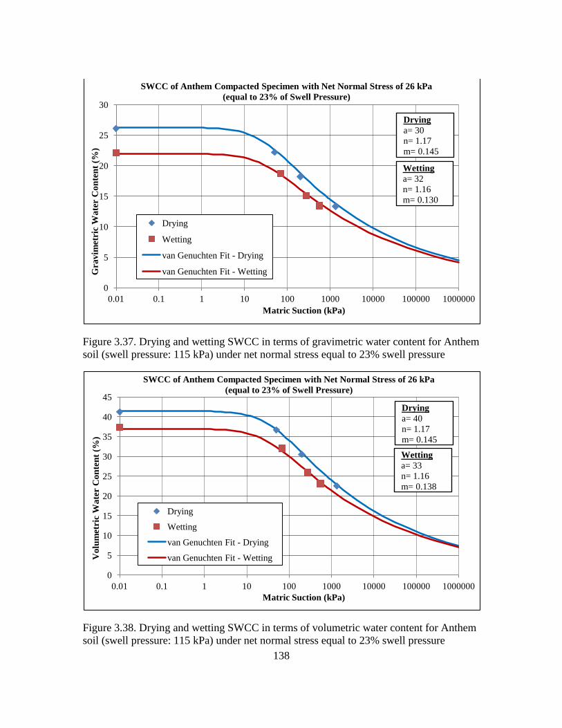
138
Figure 3.37. Drying and wetting SWCC in terms of gravimetric water content for Anthem
soil (swell pressure: 115 kPa) under net normal stress equal to 23% swell pressure
Figure 3.38. Drying and wetting SWCC in terms of volumetric water content for Anthem
soil (swell pressure: 115 kPa) under net normal stress equal to 23% swell pressure
0
5
10
15
20
25
30
0.01 0.1 1 10 100 1000 10000 100000 1000000
Gra
vim
etri
c W
ate
r C
on
ten
t (%
)
Matric Suction (kPa)
SWCC of Anthem Compacted Specimen with Net Normal Stress of 26 kPa
(equal to 23% of Swell Pressure)
Drying
Wetting
van Genuchten Fit - Drying
van Genuchten Fit - Wetting
Drying
a= 30
n= 1.17
m= 0.145
Wetting
a= 32
n= 1.16
m= 0.130
0
5
10
15
20
25
30
35
40
45
0.01 0.1 1 10 100 1000 10000 100000 1000000
Vo
lum
etri
c W
ate
r C
on
ten
t (%
)
Matric Suction (kPa)
SWCC of Anthem Compacted Specimen with Net Normal Stress of 26 kPa
(equal to 23% of Swell Pressure)
Drying
Wetting
van Genuchten Fit - Drying
van Genuchten Fit - Wetting
Drying
a= 40
n= 1.17
m= 0.145
Wetting
a= 33
n= 1.16
m= 0.138
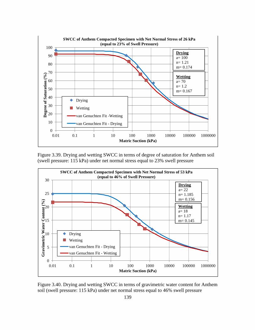
139
Figure 3.39. Drying and wetting SWCC in terms of degree of saturation for Anthem soil
(swell pressure: 115 kPa) under net normal stress equal to 23% swell pressure
Figure 3.40. Drying and wetting SWCC in terms of gravimetric water content for Anthem
soil (swell pressure: 115 kPa) under net normal stress equal to 46% swell pressure
0
10
20
30
40
50
60
70
80
90
100
0.01 0.1 1 10 100 1000 10000 100000 1000000
Deg
ree
of
Sa
tura
tio
n (
%)
Matric Suction (kPa)
SWCC of Anthem Compacted Specimen with Net Normal Stress of 26 kPa
(equal to 23% of Swell Pressure)
Drying
Wetting
van Genuchten Fit -Wetting
van Genuchten Fit - Drying
Wetting
a= 70
n= 1.2
m= 0.167
Drying
a= 100
n= 1.21
m= 0.174
0
5
10
15
20
25
30
0.01 0.1 1 10 100 1000 10000 100000 1000000
Gra
vim
etri
c W
ate
r C
on
ten
t (%
)
Matric Suction (kPa)
SWCC of Anthem Compacted Specimen with Net Normal Stress of 53 kPa
(equal to 46% of Swell Pressure)
Drying
Wetting
van Genuchten Fit - Drying
van Genuchten Fit - Wetting
Drying
a= 22
n= 1.185
m= 0.156
Wetting
a= 18
n= 1.17
m= 0.145
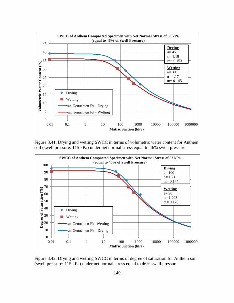
140
Figure 3.41. Drying and wetting SWCC in terms of volumetric water content for Anthem
soil (swell pressure: 115 kPa) under net normal stress equal to 46% swell pressure
Figure 3.42. Drying and wetting SWCC in terms of degree of saturation for Anthem soil
(swell pressure: 115 kPa) under net normal stress equal to 46% swell pressure
0
5
10
15
20
25
30
35
40
45
0.01 0.1 1 10 100 1000 10000 100000 1000000
Vo
lum
etri
c W
ate
r C
on
ten
t (%
)
Matric Suction (kPa)
SWCC of Anthem Compacted Specimen with Net Normal Stress of 53 kPa
(equal to 46% of Swell Pressure)
Drying
Wetting
van Genuchten Fit - Drying
van Genuchten Fit - Wetting
Drying
a= 45
n= 1.18
m= 0.153
Wetting
a= 30
n= 1.17 m= 0.145
0
10
20
30
40
50
60
70
80
90
100
0.01 0.1 1 10 100 1000 10000 100000 1000000
Deg
ree
of
Sa
tura
tio
n (
%)
Matric Suction (kPa)
SWCC of Anthem Compacted Specimen with Net Normal Stress of 53 kPa
(equal to 46% of Swell Pressure)
Drying
Wetting
van Genuchten Fit -Wetting
van Genuchten Fit - Drying
Wetting
a= 90
n= 1.205
m= 0.170
Drying
a= 100
n= 1.21
m= 0.174
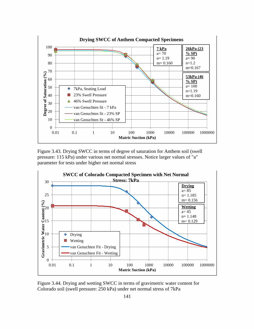
141
Figure 3.43. Drying SWCC in terms of degree of saturation for Anthem soil (swell
pressure: 115 kPa) under various net normal stresses. Notice larger values of "a"
parameter for tests under higher net normal stress
Figure 3.44. Drying and wetting SWCC in terms of gravimetric water content for
Colorado soil (swell pressure: 250 kPa) under net normal stress of 7kPa
0
10
20
30
40
50
60
70
80
90
100
0.01 0.1 1 10 100 1000 10000 100000 1000000
Deg
ree
of
Sa
tura
tio
n (
%)
Matric Suction (kPa)
Drying SWCC of Anthem Compacted Specimens
7kPa, Seating Load
23% Swell Pressure
46% Swell Pressure
van Genuchten fit - 7 kPa
van Genuchten fit - 23% SP
van Genuchten fit - 46% SP
7 kPa
a= 70
n= 1.19
m= 0.160
53kPa (46
% SP)
a= 100
n=1.19
m=0.160
26kPa (23
% SP)
a= 90
n=1.2
m=0.167
0
5
10
15
20
25
30
0.01 0.1 1 10 100 1000 10000 100000 1000000
Gra
vim
etri
c W
ate
r C
on
ten
t (%
)
Matric Suction (kPa)
SWCC of Colorado Compacted Specimen with Net Normal
Stress: 7kPa
Drying
Wetting
van Genuchten Fit - Drying
van Genuchten Fit - Wetting
Drying
a= 85
n= 1.185
m= 0.156
Wetting
a= 45
n= 1.148
m= 0.129
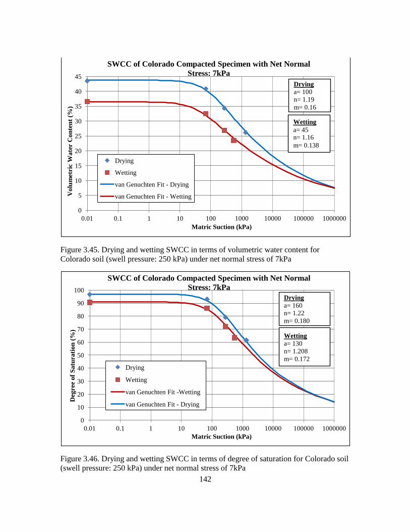
142
Figure 3.45. Drying and wetting SWCC in terms of volumetric water content for
Colorado soil (swell pressure: 250 kPa) under net normal stress of 7kPa
Figure 3.46. Drying and wetting SWCC in terms of degree of saturation for Colorado soil
(swell pressure: 250 kPa) under net normal stress of 7kPa
0
5
10
15
20
25
30
35
40
45
0.01 0.1 1 10 100 1000 10000 100000 1000000
Vo
lum
etri
c W
ate
r C
on
ten
t (%
)
Matric Suction (kPa)
SWCC of Colorado Compacted Specimen with Net Normal
Stress: 7kPa
Drying
Wetting
van Genuchten Fit - Drying
van Genuchten Fit - Wetting
Drying
a= 100
n= 1.19
m= 0.16
Wetting
a= 45 n= 1.16
m= 0.138
0
10
20
30
40
50
60
70
80
90
100
0.01 0.1 1 10 100 1000 10000 100000 1000000
Deg
ree
of
Sa
tura
tio
n (
%)
Matric Suction (kPa)
SWCC of Colorado Compacted Specimen with Net Normal
Stress: 7kPa
Drying
Wetting
van Genuchten Fit -Wetting
van Genuchten Fit - Drying
Wetting
a= 130
n= 1.208
m= 0.172
Drying
a= 160
n= 1.22
m= 0.180
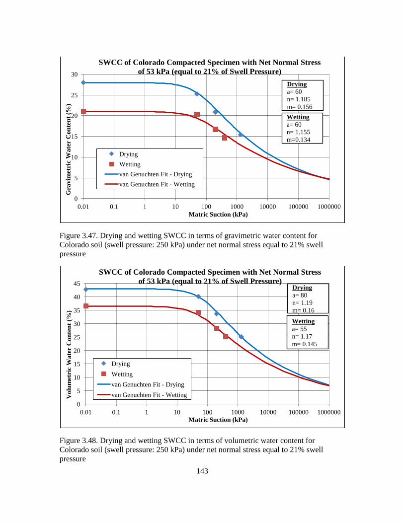
143
Figure 3.47. Drying and wetting SWCC in terms of gravimetric water content for
Colorado soil (swell pressure: 250 kPa) under net normal stress equal to 21% swell
pressure
Figure 3.48. Drying and wetting SWCC in terms of volumetric water content for
Colorado soil (swell pressure: 250 kPa) under net normal stress equal to 21% swell
pressure
0
5
10
15
20
25
30
0.01 0.1 1 10 100 1000 10000 100000 1000000
Gra
vim
etri
c W
ate
r C
on
ten
t (%
)
Matric Suction (kPa)
SWCC of Colorado Compacted Specimen with Net Normal Stress
of 53 kPa (equal to 21% of Swell Pressure)
Drying
Wetting
van Genuchten Fit - Drying
van Genuchten Fit - Wetting
Drying
a= 60
n= 1.185
m= 0.156
Wetting
a= 60
n= 1.155
m=0.134
0
5
10
15
20
25
30
35
40
45
0.01 0.1 1 10 100 1000 10000 100000 1000000
Vo
lum
etri
c W
ate
r C
on
ten
t (%
)
Matric Suction (kPa)
SWCC of Colorado Compacted Specimen with Net Normal Stress
of 53 kPa (equal to 21% of Swell Pressure)
Drying
Wetting
van Genuchten Fit - Drying
van Genuchten Fit - Wetting
Drying
a= 80
n= 1.19
m= 0.16
Wetting
a= 55
n= 1.17
m= 0.145
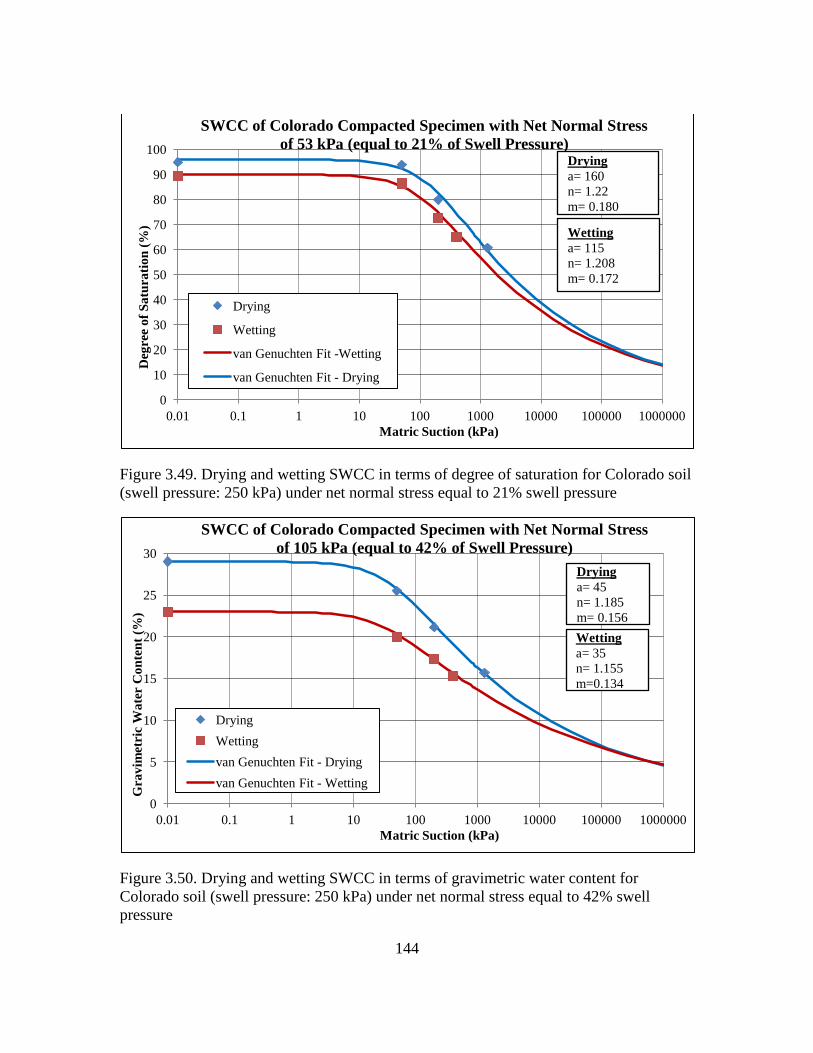
144
Figure 3.49. Drying and wetting SWCC in terms of degree of saturation for Colorado soil
(swell pressure: 250 kPa) under net normal stress equal to 21% swell pressure
Figure 3.50. Drying and wetting SWCC in terms of gravimetric water content for
Colorado soil (swell pressure: 250 kPa) under net normal stress equal to 42% swell
pressure
0
10
20
30
40
50
60
70
80
90
100
0.01 0.1 1 10 100 1000 10000 100000 1000000
Deg
ree
of
Sa
tura
tio
n (
%)
Matric Suction (kPa)
SWCC of Colorado Compacted Specimen with Net Normal Stress
of 53 kPa (equal to 21% of Swell Pressure)
Drying
Wetting
van Genuchten Fit -Wetting
van Genuchten Fit - Drying
Wetting
a= 115
n= 1.208
m= 0.172
Drying
a= 160
n= 1.22
m= 0.180
0
5
10
15
20
25
30
0.01 0.1 1 10 100 1000 10000 100000 1000000
Gra
vim
etri
c W
ate
r C
on
ten
t (%
)
Matric Suction (kPa)
SWCC of Colorado Compacted Specimen with Net Normal Stress
of 105 kPa (equal to 42% of Swell Pressure)
Drying
Wetting
van Genuchten Fit - Drying
van Genuchten Fit - Wetting
Drying
a= 45
n= 1.185
m= 0.156
Wetting
a= 35
n= 1.155
m=0.134
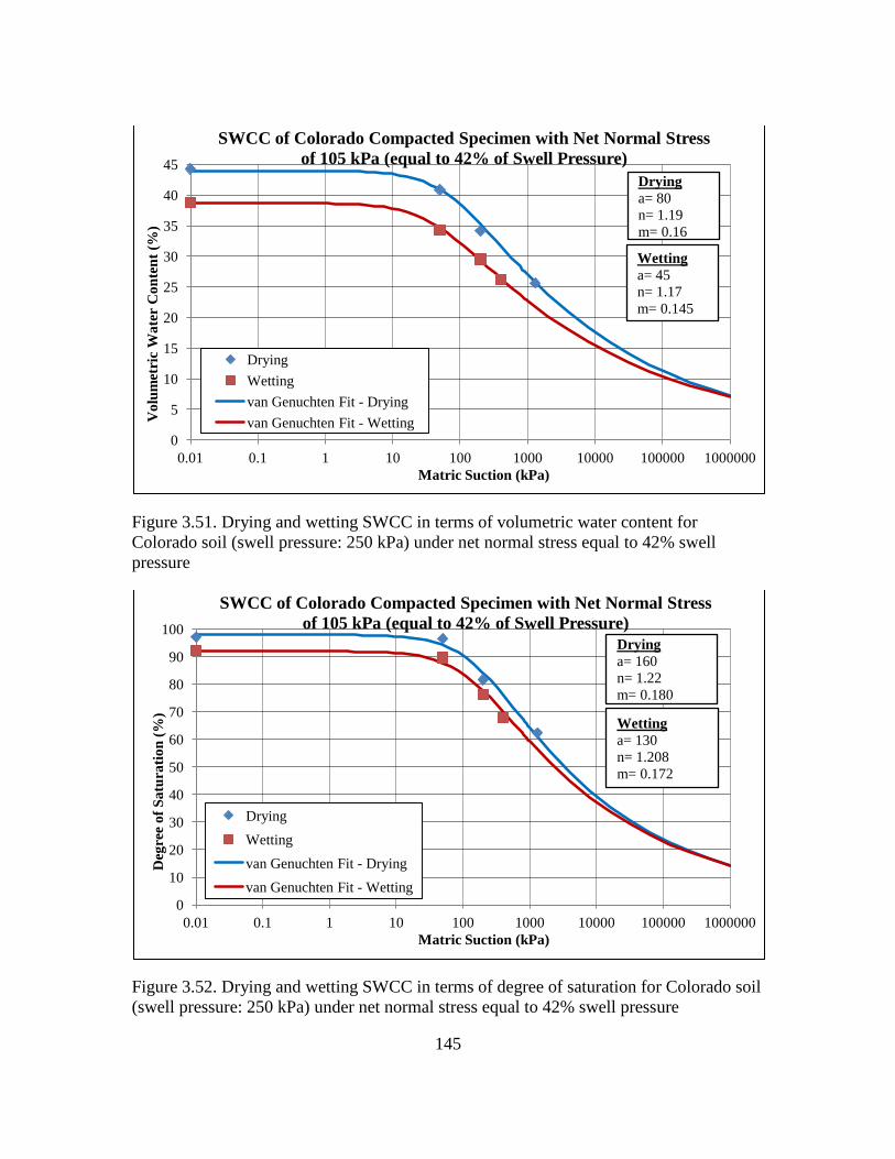
145
Figure 3.51. Drying and wetting SWCC in terms of volumetric water content for
Colorado soil (swell pressure: 250 kPa) under net normal stress equal to 42% swell
pressure
Figure 3.52. Drying and wetting SWCC in terms of degree of saturation for Colorado soil
(swell pressure: 250 kPa) under net normal stress equal to 42% swell pressure
0
5
10
15
20
25
30
35
40
45
0.01 0.1 1 10 100 1000 10000 100000 1000000
Vo
lum
etri
c W
ate
r C
on
ten
t (%
)
Matric Suction (kPa)
SWCC of Colorado Compacted Specimen with Net Normal Stress
of 105 kPa (equal to 42% of Swell Pressure)
Drying
Wetting
van Genuchten Fit - Drying
van Genuchten Fit - Wetting
Drying
a= 80
n= 1.19
m= 0.16
Wetting
a= 45
n= 1.17
m= 0.145
0
10
20
30
40
50
60
70
80
90
100
0.01 0.1 1 10 100 1000 10000 100000 1000000
Deg
ree
of
Sa
tura
tio
n (
%)
Matric Suction (kPa)
SWCC of Colorado Compacted Specimen with Net Normal Stress
of 105 kPa (equal to 42% of Swell Pressure)
Drying
Wetting
van Genuchten Fit - Drying
van Genuchten Fit - Wetting
Wetting
a= 130
n= 1.208
m= 0.172
Drying
a= 160
n= 1.22
m= 0.180
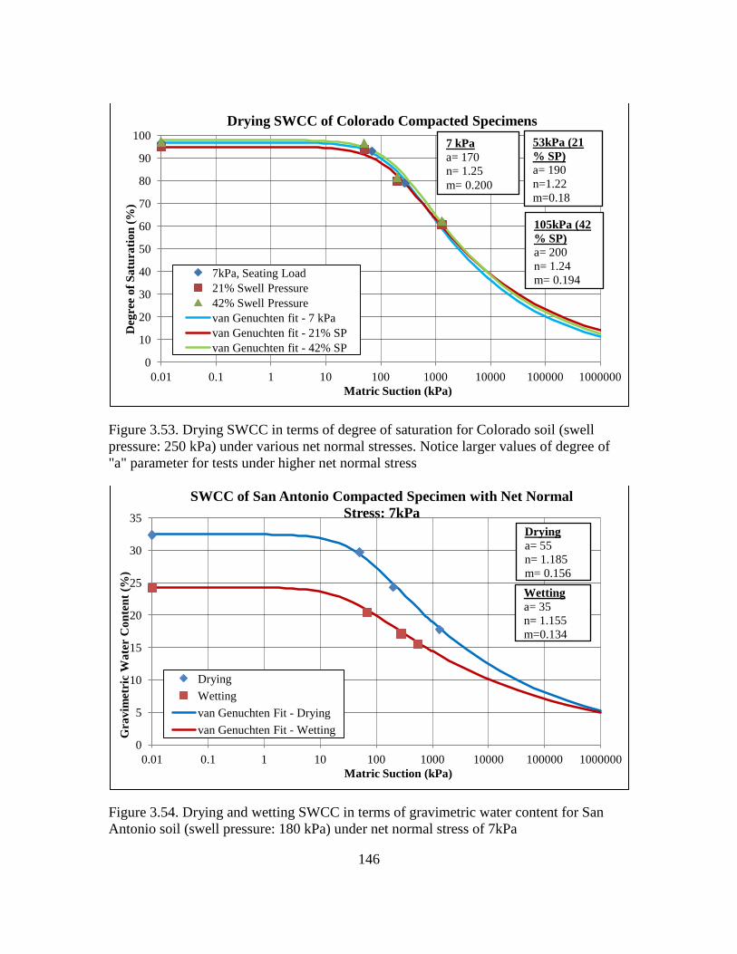
146
Figure 3.53. Drying SWCC in terms of degree of saturation for Colorado soil (swell
pressure: 250 kPa) under various net normal stresses. Notice larger values of degree of
"a" parameter for tests under higher net normal stress
Figure 3.54. Drying and wetting SWCC in terms of gravimetric water content for San
Antonio soil (swell pressure: 180 kPa) under net normal stress of 7kPa
0
10
20
30
40
50
60
70
80
90
100
0.01 0.1 1 10 100 1000 10000 100000 1000000
Deg
ree
of
Sa
tura
tio
n (
%)
Matric Suction (kPa)
Drying SWCC of Colorado Compacted Specimens
7kPa, Seating Load
21% Swell Pressure
42% Swell Pressure
van Genuchten fit - 7 kPa
van Genuchten fit - 21% SP
van Genuchten fit - 42% SP
7 kPa
a= 170
n= 1.25
m= 0.200
105kPa (42
% SP)
a= 200
n= 1.24
m= 0.194
53kPa (21
% SP)
a= 190
n=1.22
m=0.18
0
5
10
15
20
25
30
35
0.01 0.1 1 10 100 1000 10000 100000 1000000
Gra
vim
etri
c W
ate
r C
on
ten
t (%
)
Matric Suction (kPa)
SWCC of San Antonio Compacted Specimen with Net Normal
Stress: 7kPa
Drying
Wetting
van Genuchten Fit - Drying
van Genuchten Fit - Wetting
Drying
a= 55
n= 1.185
m= 0.156
Wetting
a= 35
n= 1.155
m=0.134
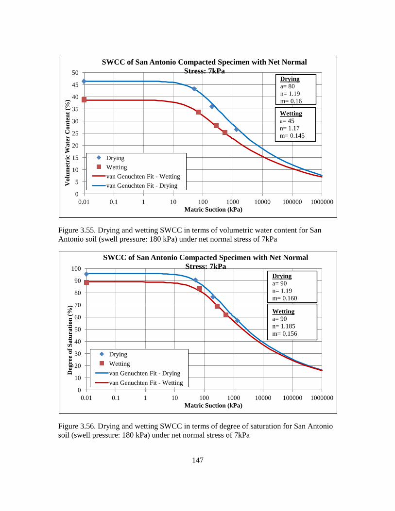
147
Figure 3.55. Drying and wetting SWCC in terms of volumetric water content for San
Antonio soil (swell pressure: 180 kPa) under net normal stress of 7kPa
Figure 3.56. Drying and wetting SWCC in terms of degree of saturation for San Antonio
soil (swell pressure: 180 kPa) under net normal stress of 7kPa
0
5
10
15
20
25
30
35
40
45
50
0.01 0.1 1 10 100 1000 10000 100000 1000000
Vo
lum
etri
c W
ate
r C
on
ten
t (%
)
Matric Suction (kPa)
SWCC of San Antonio Compacted Specimen with Net Normal
Stress: 7kPa
Drying
Wetting
van Genuchten Fit - Wetting
van Genuchten Fit - Drying
Drying
a= 80
n= 1.19
m= 0.16
Wetting
a= 45
n= 1.17
m= 0.145
0
10
20
30
40
50
60
70
80
90
100
0.01 0.1 1 10 100 1000 10000 100000 1000000
Deg
ree
of
Sa
tura
tio
n (
%)
Matric Suction (kPa)
SWCC of San Antonio Compacted Specimen with Net Normal
Stress: 7kPa
Drying
Wetting
van Genuchten Fit - Drying
van Genuchten Fit - Wetting
Wetting
a= 90
n= 1.185
m= 0.156
Drying
a= 90
n= 1.19
m= 0.160
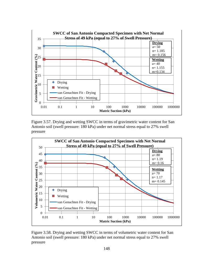
148
Figure 3.57. Drying and wetting SWCC in terms of gravimetric water content for San
Antonio soil (swell pressure: 180 kPa) under net normal stress equal to 27% swell
pressure
Figure 3.58. Drying and wetting SWCC in terms of volumetric water content for San
Antonio soil (swell pressure: 180 kPa) under net normal stress equal to 27% swell
pressure
0
5
10
15
20
25
30
35
0.01 0.1 1 10 100 1000 10000 100000 1000000
Gra
vim
etri
c W
ate
r C
on
ten
t (%
)
Matric Suction (kPa)
SWCC of San Antonio Compacted Specimen with Net Normal
Stress of 49 kPa (equal to 27% of Swell Pressure)
Drying
Wetting
van Genuchten Fit - Drying
van Genuchten Fit - Wetting
Drying
a= 50
n= 1.185
m= 0.156
Wetting
a= 40
n= 1.155
m=0.134
0
5
10
15
20
25
30
35
40
45
50
0.01 0.1 1 10 100 1000 10000 100000 1000000
Vo
lum
etri
c W
ate
r C
on
ten
t (%
)
Matric Suction (kPa)
SWCC of San Antonio Compacted Specimen with Net Normal
Stress of 49 kPa (equal to 27% of Swell Pressure)
Drying
Wetting
van Genuchten Fit - Drying
van Genuchten Fit - Wetting
Drying
a= 80
n= 1.19
m= 0.16
Wetting
a= 70
n= 1.17
m= 0.145
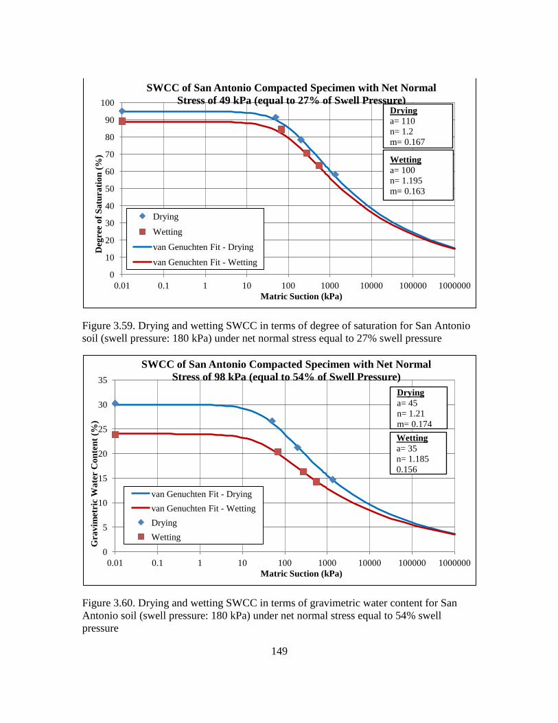
149
Figure 3.59. Drying and wetting SWCC in terms of degree of saturation for San Antonio
soil (swell pressure: 180 kPa) under net normal stress equal to 27% swell pressure
Figure 3.60. Drying and wetting SWCC in terms of gravimetric water content for San
Antonio soil (swell pressure: 180 kPa) under net normal stress equal to 54% swell
pressure
0
10
20
30
40
50
60
70
80
90
100
0.01 0.1 1 10 100 1000 10000 100000 1000000
Deg
ree
of
Sa
tura
tio
n (
%)
Matric Suction (kPa)
SWCC of San Antonio Compacted Specimen with Net Normal
Stress of 49 kPa (equal to 27% of Swell Pressure)
Drying
Wetting
van Genuchten Fit - Drying
van Genuchten Fit - Wetting
Wetting
a= 100
n= 1.195
m= 0.163
Drying
a= 110
n= 1.2
m= 0.167
0
5
10
15
20
25
30
35
0.01 0.1 1 10 100 1000 10000 100000 1000000
Gra
vim
etri
c W
ate
r C
on
ten
t (%
)
Matric Suction (kPa)
SWCC of San Antonio Compacted Specimen with Net Normal
Stress of 98 kPa (equal to 54% of Swell Pressure)
van Genuchten Fit - Drying
van Genuchten Fit - Wetting
Drying
Wetting
Drying
a= 45
n= 1.21
m= 0.174
Wetting
a= 35
n= 1.185
0.156
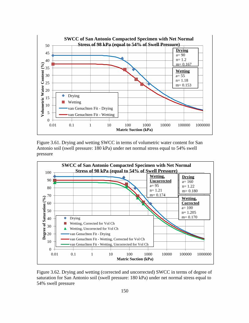
150
Figure 3.61. Drying and wetting SWCC in terms of volumetric water content for San
Antonio soil (swell pressure: 180 kPa) under net normal stress equal to 54% swell
pressure
Figure 3.62. Drying and wetting (corrected and uncorrected) SWCC in terms of degree of
saturation for San Antonio soil (swell pressure: 180 kPa) under net normal stress equal to
54% swell pressure
0
5
10
15
20
25
30
35
40
45
50
0.01 0.1 1 10 100 1000 10000 100000 1000000
Vo
lum
etri
c W
ate
r C
on
ten
t (%
)
Matric Suction (kPa)
SWCC of San Antonio Compacted Specimen with Net Normal
Stress of 98 kPa (equal to 54% of Swell Pressure)
Drying
Wetting
van Genuchten Fit - Drying
van Genuchten Fit - Wetting
Drying
a= 90
n= 1.2
m= 0.167
Wetting
a= 55
n= 1.18
m= 0.153
0
10
20
30
40
50
60
70
80
90
100
0.01 0.1 1 10 100 1000 10000 100000 1000000
Deg
ree
of
Sa
tura
tio
n (
%)
Matric Suction (kPa)
SWCC of San Antonio Compacted Specimen with Net Normal
Stress of 98 kPa (equal to 54% of Swell Pressure)
Drying
Wetting, Corrected for Vol Ch
Wetting, Uncorrected for Vol Ch
van Genuchten Fit - Drying
van Genuchten Fit - Wetting, Corrected for Vol Ch
van Genuchten Fit - Wetting, Uncorrected for Vol Ch
Wetting,
Corrected
a= 100
n= 1.205
m= 0.170
Drying
a= 160
n= 1.22
m= 0.180
Wetting,
Uncorrected
a= 95
n= 1.21
m= 0.174
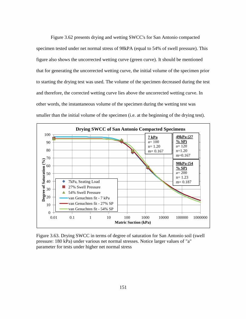
151
Figure 3.62 presents drying and wetting SWCC's for San Antonio compacted
specimen tested under net normal stress of 98kPA (equal to 54% of swell pressure). This
figure also shows the uncorrected wetting curve (green curve). It should be mentioned
that for generating the uncorrected wetting curve, the initial volume of the specimen prior
to starting the drying test was used. The volume of the specimen decreased during the test
and therefore, the corrected wetting curve lies above the uncorrected wetting curve. In
other words, the instantaneous volume of the specimen during the wetting test was
smaller than the initial volume of the specimen (i.e. at the beginning of the drying test).
Figure 3.63. Drying SWCC in terms of degree of saturation for San Antonio soil (swell
pressure: 180 kPa) under various net normal stresses. Notice larger values of "a"
parameter for tests under higher net normal stress
0
10
20
30
40
50
60
70
80
90
100
0.01 0.1 1 10 100 1000 10000 100000 1000000
Deg
ree
of
Sa
tura
tio
n (
%)
Matric Suction (kPa)
Drying SWCC of San Antonio Compacted Specimens
7kPa, Seating Load
27% Swell Pressure
54% Swell Pressure
van Genuchten fit - 7 kPa
van Genuchten fit - 27% SP
van Genuchten fit - 54% SP
7 kPa
a= 100
n= 1.20
m= 0.167
98kPa (54
% SP)
a= 200
n= 1.23
m= 0.187
49kPa (27
% SP)
a= 120
n=1.20
m=0.167
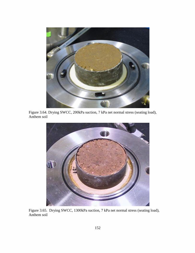
152
Figure 3.64. Drying SWCC, 200kPa suction, 7 kPa net normal stress (seating load),
Anthem soil
Figure 3.65. Drying SWCC, 1300kPa suction, 7 kPa net normal stress (seating load),
Anthem soil
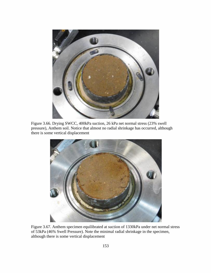
153
Figure 3.66. Drying SWCC, 400kPa suction, 26 kPa net normal stress (23% swell
pressure), Anthem soil. Notice that almost no radial shrinkage has occurred, although
there is some vertical displacement
Figure 3.67. Anthem specimen equilibrated at suction of 1330kPa under net normal stress
of 53kPa (46% Swell Pressure). Note the minimal radial shrinkage in the specimen,
although there is some vertical displacement
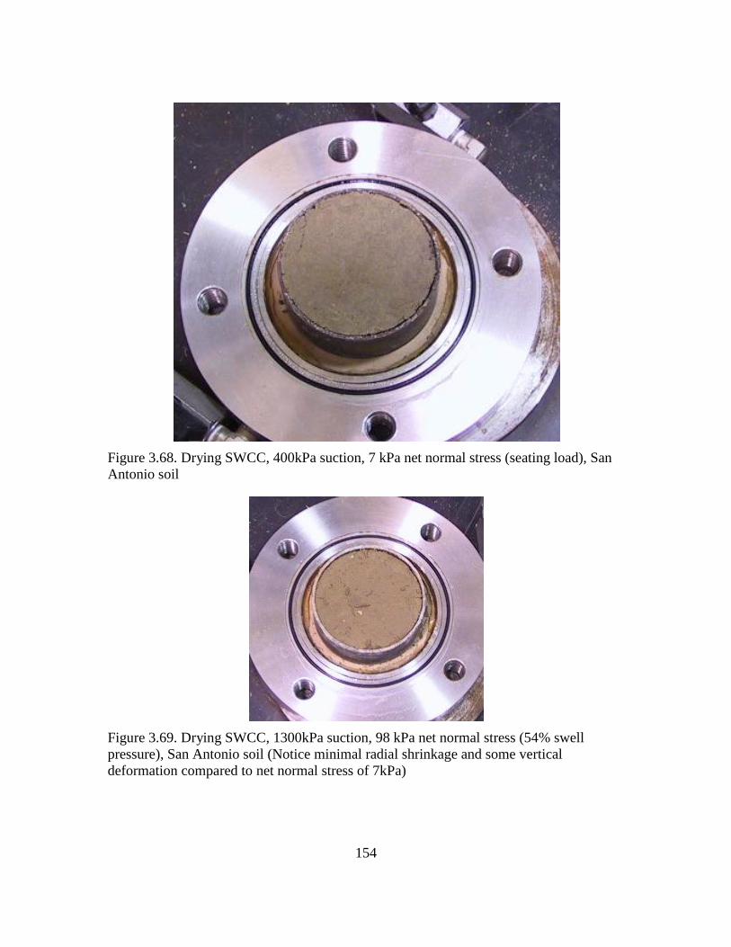
154
Figure 3.68. Drying SWCC, 400kPa suction, 7 kPa net normal stress (seating load), San
Antonio soil
Figure 3.69. Drying SWCC, 1300kPa suction, 98 kPa net normal stress (54% swell
pressure), San Antonio soil (Notice minimal radial shrinkage and some vertical
deformation compared to net normal stress of 7kPa)
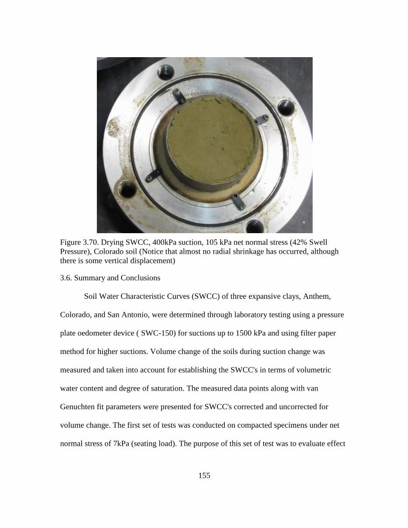
155
Figure 3.70. Drying SWCC, 400kPa suction, 105 kPa net normal stress (42% Swell
Pressure), Colorado soil (Notice that almost no radial shrinkage has occurred, although
there is some vertical displacement)
3.6. Summary and Conclusions
Soil Water Characteristic Curves (SWCC) of three expansive clays, Anthem,
Colorado, and San Antonio, were determined through laboratory testing using a pressure
plate oedometer device ( SWC-150) for suctions up to 1500 kPa and using filter paper
method for higher suctions. Volume change of the soils during suction change was
measured and taken into account for establishing the SWCC's in terms of volumetric
water content and degree of saturation. The measured data points along with van
Genuchten fit parameters were presented for SWCC's corrected and uncorrected for
volume change. The first set of tests was conducted on compacted specimens under net
normal stress of 7kPa (seating load). The purpose of this set of test was to evaluate effect
156
of considering soil volume change on the shape of SWCC of expansive clays, with
particular focus on the air-entry value.
Another set of tests were conducted in which slurry specimens of the soils were
tested. The slurry specimens were prepared by mixing certain amount of soil and water to
make sure that the specimen had reached 100% saturation. The effect of initial state of
the specimen on its SWCC was studied by this set of experiments. It was found that
slurry specimens undergo significant volume changes during SWCC test. Therefore, the
difference between the volume corrected SWCC and uncorrected SWCC was more
significant for slurry specimens compared to compacted.
The last set of laboratory experiments were intended to help evaluate the effect of
net normal stress on the volume change of specimens and its impact on the shape of
SWCC. For this set of experiments, different net normal stresses were used. The range of
net normal stresses was from 7kPa to around 55% of the swell pressure of the tested soil.
Volume corrected SWCC's were developed by using the instantaneous volume of
the specimen while in volume uncorrected SWCC's initial volume of the specimen was
used and the soil volume change throughout the test was ignored.
It was found that volume change consideration plays a major role in shape of the
SWCC particularly regarding the air-entry value (AEV) and slope in the transition zone.
The air-entry value was shown to be larger for volume-corrected SWCC's compared to
volume-uncorrected SWCC's. The slope of the curve in the transition zone also showed
higher values for corrected SWCC's. These are shown in Figure 3.71 for Colorado soil.
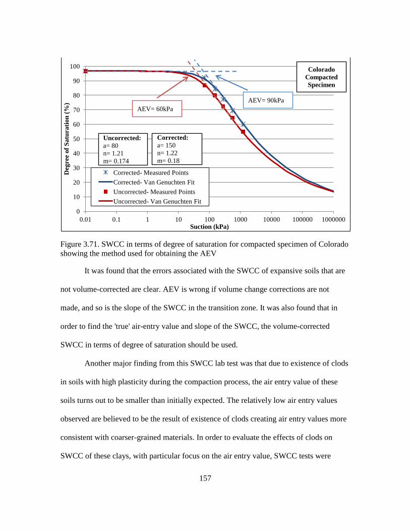
157
Figure 3.71. SWCC in terms of degree of saturation for compacted specimen of Colorado
showing the method used for obtaining the AEV
It was found that the errors associated with the SWCC of expansive soils that are
not volume-corrected are clear. AEV is wrong if volume change corrections are not
made, and so is the slope of the SWCC in the transition zone. It was also found that in
order to find the 'true' air-entry value and slope of the SWCC, the volume-corrected
SWCC in terms of degree of saturation should be used.
Another major finding from this SWCC lab test was that due to existence of clods
in soils with high plasticity during the compaction process, the air entry value of these
soils turns out to be smaller than initially expected. The relatively low air entry values
observed are believed to be the result of existence of clods creating air entry values more
consistent with coarser-grained materials. In order to evaluate the effects of clods on
SWCC of these clays, with particular focus on the air entry value, SWCC tests were
0
10
20
30
40
50
60
70
80
90
100
0.01 0.1 1 10 100 1000 10000 100000 1000000
Deg
ree
of
Sa
tura
tio
n (
%)
Suction (kPa)
Corrected- Measured Points
Corrected- Van Genuchten Fit
Uncorrected- Measured Points
Uncorrected- Van Genuchten Fit
Corrected:
a= 150
n= 1.22
m= 0.18
Uncorrected:
a= 80
n= 1.21
m= 0.174
AEV= 90kPa
AEV= 60kPa
Colorado
Compacted
Specimen
158
performed on slurry specimens. In slurry specimens, the pulverized soil was entirely
saturated with water and therefore clods did not appear within the specimen.
Slurry specimens of Anthem, Colorado, and San Antonio soils were tested and the
resulting SWCC's were compared against the SWCC's obtained from the compacted
specimens of the same soils. It was found that initial state of the specimen has a
significant effect on the shape of the SWCC, particularly due to high volume change of
slurry specimens during the test. For any given soil tested, the air-entry value of volume-
corrected SWCC's obtained from testing slurry specimens was found to be higher than
that of compacted specimens. The slope in transition zone was also found to be higher for
slurry specimens. It was found that Slurry specimens showed generally larger AEV
compared to compacted due to a combination of volume change and structure effects.
Figure 3.72 presents SWCC in terms of degree of saturation including both corrected and
uncorrected curves for slurry specimen of San Antonio soil. The significant difference in
AEV and slope in the transition zone between corrected and uncorrected curves are
presented in this figure.
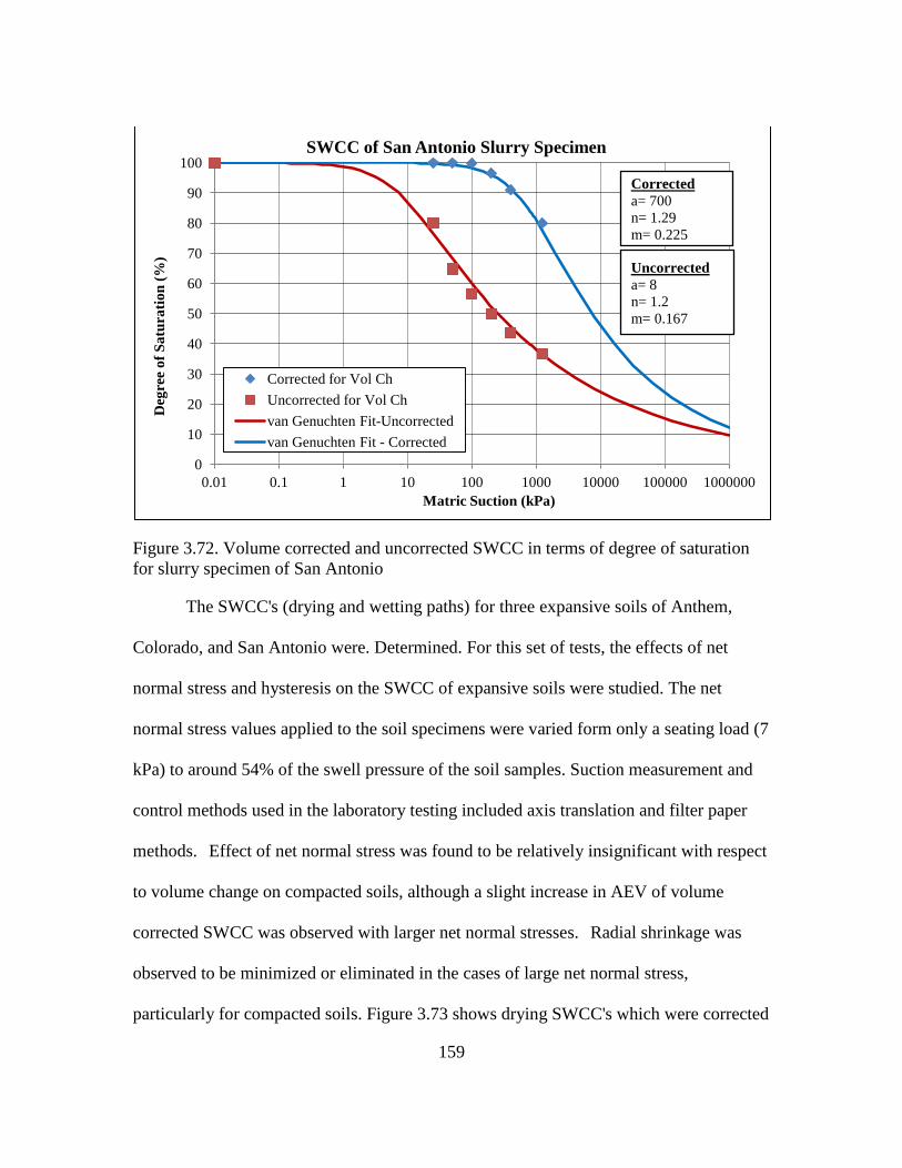
159
Figure 3.72. Volume corrected and uncorrected SWCC in terms of degree of saturation
for slurry specimen of San Antonio
The SWCC's (drying and wetting paths) for three expansive soils of Anthem,
Colorado, and San Antonio were. Determined. For this set of tests, the effects of net
normal stress and hysteresis on the SWCC of expansive soils were studied. The net
normal stress values applied to the soil specimens were varied form only a seating load (7
kPa) to around 54% of the swell pressure of the soil samples. Suction measurement and
control methods used in the laboratory testing included axis translation and filter paper
methods. Effect of net normal stress was found to be relatively insignificant with respect
to volume change on compacted soils, although a slight increase in AEV of volume
corrected SWCC was observed with larger net normal stresses. Radial shrinkage was
observed to be minimized or eliminated in the cases of large net normal stress,
particularly for compacted soils. Figure 3.73 shows drying SWCC's which were corrected
0
10
20
30
40
50
60
70
80
90
100
0.01 0.1 1 10 100 1000 10000 100000 1000000
Deg
ree
of
Sa
tura
tio
n (
%)
Matric Suction (kPa)
SWCC of San Antonio Slurry Specimen
Corrected for Vol Ch
Uncorrected for Vol Ch
van Genuchten Fit-Uncorrected
van Genuchten Fit - Corrected
Uncorrected
a= 8
n= 1.2
m= 0.167
Corrected
a= 700
n= 1.29
m= 0.225
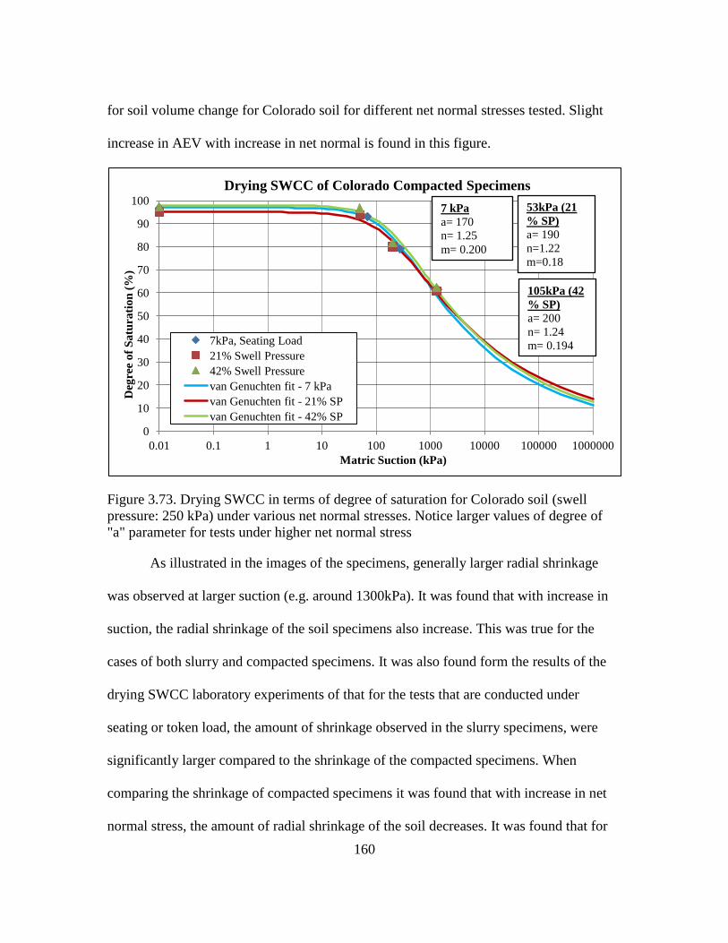
160
for soil volume change for Colorado soil for different net normal stresses tested. Slight
increase in AEV with increase in net normal is found in this figure.
Figure 3.73. Drying SWCC in terms of degree of saturation for Colorado soil (swell
pressure: 250 kPa) under various net normal stresses. Notice larger values of degree of
"a" parameter for tests under higher net normal stress
As illustrated in the images of the specimens, generally larger radial shrinkage
was observed at larger suction (e.g. around 1300kPa). It was found that with increase in
suction, the radial shrinkage of the soil specimens also increase. This was true for the
cases of both slurry and compacted specimens. It was also found form the results of the
drying SWCC laboratory experiments of that for the tests that are conducted under
seating or token load, the amount of shrinkage observed in the slurry specimens, were
significantly larger compared to the shrinkage of the compacted specimens. When
comparing the shrinkage of compacted specimens it was found that with increase in net
normal stress, the amount of radial shrinkage of the soil decreases. It was found that for
0
10
20
30
40
50
60
70
80
90
100
0.01 0.1 1 10 100 1000 10000 100000 1000000
Deg
ree
of
Sa
tura
tio
n (
%)
Matric Suction (kPa)
Drying SWCC of Colorado Compacted Specimens
7kPa, Seating Load
21% Swell Pressure
42% Swell Pressure
van Genuchten fit - 7 kPa
van Genuchten fit - 21% SP
van Genuchten fit - 42% SP
7 kPa
a= 170
n= 1.25
m= 0.200
105kPa (42
% SP)
a= 200
n= 1.24
m= 0.194
53kPa (21
% SP)
a= 190
n=1.22
m=0.18

161
the compacted specimens which were tested under large amounts of net normal stress
(e.g. around 50% of the swell pressure of the soil) the radial shrinkage of the soil during
the drying SWCC test was minimal such that the contact between the soil and the
confining ring was maintained throughout the test even at relatively large suction values
(i.e. around 1300 kPa). For such cases in which the contact between the soil and the
confining ring is maintained throughout the test, it can be assumed the volume change of
the soil is only in the vertical direction. This volume change can be measured much easier
and with more accuracy. Of course, when the path is wetting rather than drying, there is
no shrinkage issue to deal with in determining the SWCC.
162
Chapter 4
NUMERICAL MODELING OF EXPANSIVE CLAYS
4.1. Introduction
In the previous chapters it shown that correcting SWCC's for soil volume change
can have a significant impact on the shape of the SWCC, particularly its air entry value
(AEV) and slope in the transition zone (i.e. suction between AEV and residual). Since
correcting for volume change alters the shape, slope and air entry value of the SWCC,
considerable differences may appear between changes in suction in the soil with the
SWCC corrected for volume change compared to that obtained with the uncorrected
SWCC. Studies that capture the importance of correcting SWCC's for soil volume change
through numerical modeling of water flow through soils, including its impact on the
resulting soil deformations (e.g. expansion/shrinkage of expansive soils) could not be
found through literature research, and thus this study represents a new contribution to the
state of knowledge of moisture movement through expansive soils and associated
deformations.
In a study conducted by GEO-SLOPE International Ltd. (2012), sensitivity of
hydraulic simulation results to some material properties was evaluated, including a
sensitivity study on air-entry value of soils found from SWCC. In order to find the
sensitivity of unsaturated flow results to air-entry value (AEV), the authors changed AEV
of a soil from 3kPa to 10kPa and kept the rest of the parameters constant. The authors
found rather considerable difference in results of the analyses, as shown in Figures 4.1
and 4.2. The difference in capillary rise was evaluated for the two air entry values of
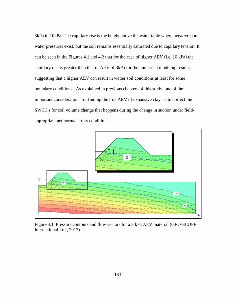
163
3kPa to 10kPa. The capillary rise is the height above the water table where negative pore-
water pressures exist, but the soil remains essentially saturated due to capillary tension. It
can be seen in the Figures 4.1 and 4.2 that for the case of higher AEV (i.e. 10 kPa) the
capillary rise is greater than that of AEV of 3kPa for the numerical modeling results,
suggesting that a higher AEV can result in wetter soil conditions at least for some
boundary conditions. As explained in previous chapters of this study, one of the
important considerations for finding the true AEV of expansive clays is to correct the
SWCC's for soil volume change that happens during the change in suction under field-
appropriate net normal stress conditions.
Figure 4.1. Pressure contours and flow vectors for a 3 kPa AEV material (GEO-SLOPE
International Ltd., 2012)
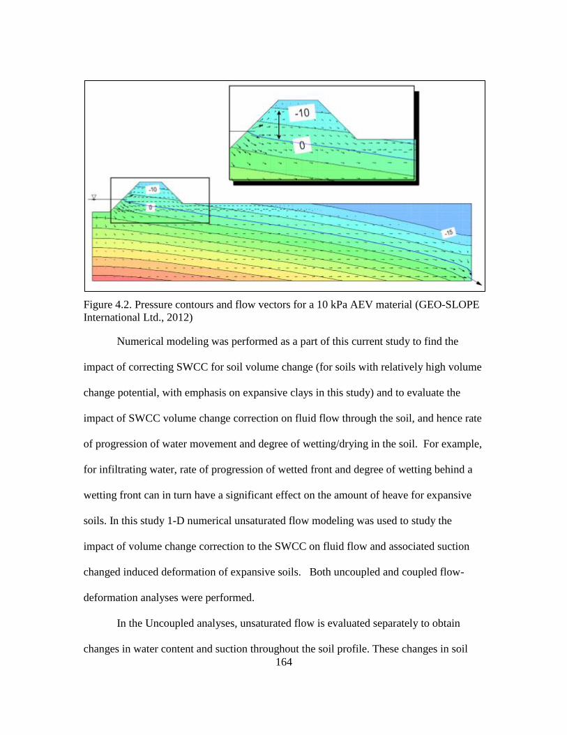
164
Figure 4.2. Pressure contours and flow vectors for a 10 kPa AEV material (GEO-SLOPE
International Ltd., 2012)
Numerical modeling was performed as a part of this current study to find the
impact of correcting SWCC for soil volume change (for soils with relatively high volume
change potential, with emphasis on expansive clays in this study) and to evaluate the
impact of SWCC volume change correction on fluid flow through the soil, and hence rate
of progression of water movement and degree of wetting/drying in the soil. For example,
for infiltrating water, rate of progression of wetted front and degree of wetting behind a
wetting front can in turn have a significant effect on the amount of heave for expansive
soils. In this study 1-D numerical unsaturated flow modeling was used to study the
impact of volume change correction to the SWCC on fluid flow and associated suction
changed induced deformation of expansive soils. Both uncoupled and coupled flow-
deformation analyses were performed.
In the Uncoupled analyses, unsaturated flow is evaluated separately to obtain
changes in water content and suction throughout the soil profile. These changes in soil
165
suction are subsequently used to compute soil deformations using a separate stress-
deformation analysis. In the Coupled flow-deformation analyses, however, the governing
partial differential equations for flow and deformation are combined such that flow of
water through soil and also the amount of deformation caused by change in suction of the
soil are solved for simultaneously. In other words, the flow-deformation analyses is
performed such that the effect of suction change induced deformations on overall stress
state is taken into account and the effect of stress change (e.g. net normal stress or
suction) on deformation are taken into account as flow progresses.
Three computer programs of VADOSE/W, CODE-BRIGHT, and SVFLUX were
used to evaluate the effect of correcting SWCC's on fluid flow through the unsaturated
expansive clay soils. The resulting amount of expansion/shrinkage was subsequently
determined, either in a decouple manner (using volume change computations done by
hand) or by couple analyses (e.g. using CODE-BRIGHT). These unsaturated flow
computer codes have the capability of simulating saturated and unsaturated flow of water
through soils, although the emphasis in this study was on unsaturated flow, defined here
as fluid flow through soils under negative pore water pressure (soil suction) conditions.
The relatively simple CAD-based user interface of all three programs can be used to
create the models effectively. During the modeling study, effect of considering volume
change on hydraulic properties of the unsaturated soils with respect to fluid flow
modeling and rate of advancement of wetted or drying front and suction change induced
volume change in expansive soils within the profile were assessed. Although most of
the analyses considered a wetting front, some cases of evaporation (drying) were
166
performed to obtain the results over a wider range of surface flux boundary conditions
and associated suction profile cases. The laboratory results obtained from SWCC tests
on three expansive soils of Anthem, Colorado, and San Antonio were used in the
unsaturated flow modeling, and laboratory-measured suction compression indices on
these soils were used for the stress-deformation computations (suction-changed induced
volume change computations). One dimensional moisture movement through an
expansive soil, using the same initial conditions and boundary conditions, was simulated
once with the SWCC corrected and once with the SWCC uncorrected for volume change.
To simulate the one-dimensional flow, geometry of 1m x 50m representing a column of
soil was used. The next step in the modeling process was to define the material
properties.
Regarding the material properties used, two separate models were created for: (1)
SWCC corrected and (2) SWCC uncorrected for soil volume change. In the two models,
all other material properties (e.g. saturated hydraulic conductivity), and all the boundary
conditions were kept the same. As it was concluded from the previous chapters of this
study (i.e. through literature search and laboratory testing), the SWCC in terms of degree
of saturation (as opposed to SWCC in terms of gravimetric and volumetric water content)
best illustrates the water retention characteristics of the soil (particularly its AEV),
especially for soils with high volume change potential. However, VADOSE/W and
SVFLUX only allow SWCC's to be entered in terms of volumetric water content.
Therefore, the data points from the corrected and uncorrected SWCC in terms of
volumetric water content were used in VADOSE/W and SVFLUX. On the other hand,
167
CODE-BRIGHT only allows SWCC's in terms of degree of saturation, and therefore, for
modeling in CODE-BRIGHT, SWCC's in terms of degree of saturation were used.
Two types of analyses were done for the soils in this study: (1) Steady-State, and
(2) Transient. In this study, the majority of simulations were carried out by steady-state
analysis due to its simplicity and much shorter solution times compared to the transient
flow analysis. A few transient analyses were also conducted in order to evaluate the
progress of the model towards the steady-state condition and to study the impact of
volume change corrections at intermediate stages of flow. The intermediate stages of
flow are expected to exhibit at least some significant difference, perhaps even in trends
(direction) of difference between corrected and uncorrected flow analyses results, due to
the highly nonlinear nature of the unsaturated flow properties, particularly in the
transition zone range of the SWCC.
Steady-State refers to a condition in which the flow through the soil has become
steady and no change in the fluid potential condition occurs over time. In other words, in
a steady-state analysis, the amount of flow into the system corresponds to the flow rate
out of the system. A steady state analysis does not consider how long it takes to achieve a
steady condition – the solution is to the homogenous form of the unsaturated flow partial
differential equation. For steady state, it is implied that the boundary values have been in
place forever and will be in place forever (Geo-Slope International, 2012).
For the case of transient flow, however, the condition of the domain is not
constant and changes with time. The flow into the system may be different from the flow
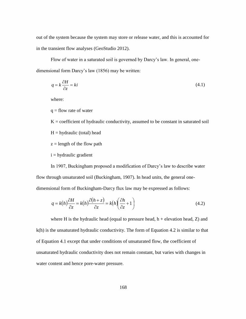
168
out of the system because the system may store or release water, and this is accounted for
in the transient flow analyses (GeoStudio 2012).
Flow of water in a saturated soil is governed by Darcy’s law. In general, one-
dimensional form Darcy’s law (1856) may be written:
kiz
Hkq
(4.1)
where:
q = flow rate of water
K = coefficient of hydraulic conductivity, assumed to be constant in saturated soil
H = hydraulic (total) head
z = length of the flow path
i = hydraulic gradient
In 1907, Buckingham proposed a modification of Darcy’s law to describe water
flow through unsaturated soil (Buckingham, 1907). In head units, the general one-
dimensional form of Buckingham-Darcy flux law may be expressed as follows:
1
z
hhk
z
zhhk
z
Hhkq (4.2)
where H is the hydraulic head (equal to pressure head, h + elevation head, Z) and
k(h) is the unsaturated hydraulic conductivity. The form of Equation 4.2 is similar to that
of Equation 4.1 except that under conditions of unsaturated flow, the coefficient of
unsaturated hydraulic conductivity does not remain constant, but varies with changes in
water content and hence pore-water pressure.
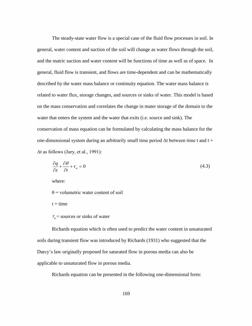
169
The steady-state water flow is a special case of the fluid flow processes in soil. In
general, water content and suction of the soil will change as water flows through the soil,
and the matric suction and water content will be functions of time as well as of space. In
general, fluid flow is transient, and flows are time-dependent and can be mathematically
described by the water mass balance or continuity equation. The water mass balance is
related to water flux, storage changes, and sources or sinks of water. This model is based
on the mass conservation and correlates the change in mater storage of the domain to the
water that enters the system and the water that exits (i.e. source and sink). The
conservation of mass equation can be formulated by calculating the mass balance for the
one-dimensional system during an arbitrarily small time period Δt between time t and t +
Δt as follows (Jury, et al., 1991):
0
wr
tz
q (4.3)
where:
θ = volumetric water content of soil
t = time
wr = sources or sinks of water
Richards equation which is often used to predict the water content in unsaturated
soils during transient flow was introduced by Richards (1931) who suggested that the
Darcy’s law originally proposed for saturated flow in porous media can also be
applicable to unsaturated flow in porous media.
Richards equation can be presented in the following one-dimensional form:
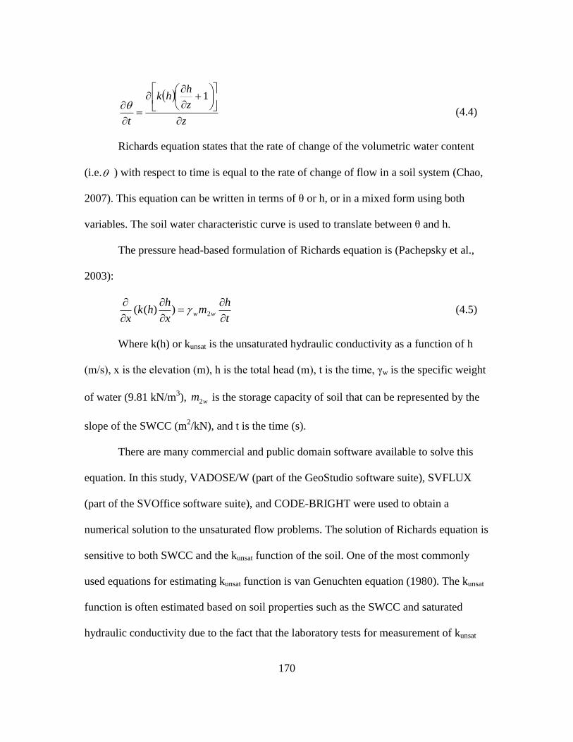
170
z
z
hhk
t
1
(4.4)
Richards equation states that the rate of change of the volumetric water content
(i.e. ) with respect to time is equal to the rate of change of flow in a soil system (Chao,
2007). This equation can be written in terms of θ or h, or in a mixed form using both
variables. The soil water characteristic curve is used to translate between θ and h.
The pressure head-based formulation of Richards equation is (Pachepsky et al.,
2003):
t
hm
x
hhk
xww
2))(( (4.5)
Where k(h) or kunsat is the unsaturated hydraulic conductivity as a function of h
(m/s), x is the elevation (m), h is the total head (m), t is the time, γw is the specific weight
of water (9.81 kN/m3), wm2 is the storage capacity of soil that can be represented by the
slope of the SWCC (m2/kN), and t is the time (s).
There are many commercial and public domain software available to solve this
equation. In this study, VADOSE/W (part of the GeoStudio software suite), SVFLUX
(part of the SVOffice software suite), and CODE-BRIGHT were used to obtain a
numerical solution to the unsaturated flow problems. The solution of Richards equation is
sensitive to both SWCC and the kunsat function of the soil. One of the most commonly
used equations for estimating kunsat function is van Genuchten equation (1980). The kunsat
function is often estimated based on soil properties such as the SWCC and saturated
hydraulic conductivity due to the fact that the laboratory tests for measurement of kunsat

171
are generally costly and time consuming. The SWCC and the kunsat function are both
sensitive to volume change of the soil that occurs in response suction change under a
particular set of net normal stress conditions.
Finite element numerical methods (such as models embedded in computer
programs VADOSE/W, SVFLUX, and CODE-BRIGHT) are based on the concept of
subdividing a continuum into small pieces, describing the behavior or actions of the
individual pieces and then reconnecting all the pieces to represent the behavior of the
continuum as a whole (GeoStudio, 2012). This process of subdividing the continuum into
smaller pieces is known as discretization or meshing. The pieces are known as finite
elements or mesh. In order to make sure that the results are accurate, it is important to set
the mesh equal to or smaller than the optimum size. Some programs (e.g. SVFLUX
provide the user with the option of automatic mesh size optimization) while other
program do not provide this feature (e.g. VADOSE/W). for the programs that do not do
the automatic mesh size optimization, the user need to make sure to find the optimum
mesh size for stability and convergence through trial and error. Discretization (mesh size
selection) is a critical element of finite element modeling. In addition, defining material
properties and boundary conditions are critical elements(GeoStudio, 2012)It is also
important to investigate, through trial and error, the extent of the domain boundaries such
that placement of the boundaries does not affect the solution in regions of primary
interest for the problem.
The primary steps to create and analyze a model using VADOSE/W, SVFLUX,
and CODE-BRIGHT are as follows:
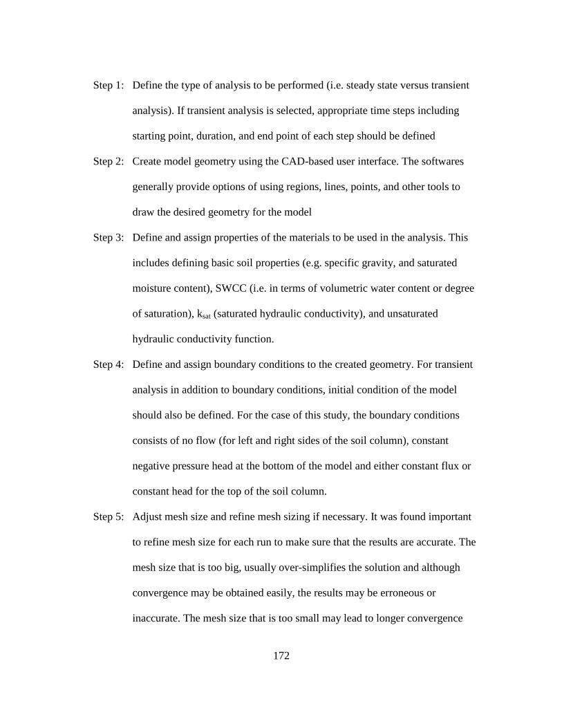
172
Step 1: Define the type of analysis to be performed (i.e. steady state versus transient
analysis). If transient analysis is selected, appropriate time steps including
starting point, duration, and end point of each step should be defined
Step 2: Create model geometry using the CAD-based user interface. The softwares
generally provide options of using regions, lines, points, and other tools to
draw the desired geometry for the model
Step 3: Define and assign properties of the materials to be used in the analysis. This
includes defining basic soil properties (e.g. specific gravity, and saturated
moisture content), SWCC (i.e. in terms of volumetric water content or degree
of saturation), ksat (saturated hydraulic conductivity), and unsaturated
hydraulic conductivity function.
Step 4: Define and assign boundary conditions to the created geometry. For transient
analysis in addition to boundary conditions, initial condition of the model
should also be defined. For the case of this study, the boundary conditions
consists of no flow (for left and right sides of the soil column), constant
negative pressure head at the bottom of the model and either constant flux or
constant head for the top of the soil column.
Step 5: Adjust mesh size and refine mesh sizing if necessary. It was found important
to refine mesh size for each run to make sure that the results are accurate. The
mesh size that is too big, usually over-simplifies the solution and although
convergence may be obtained easily, the results may be erroneous or
inaccurate. The mesh size that is too small may lead to longer convergence
173
time which is not always necessary, with the numerical solutions the same as
the ones in which the optimum mesh size has been used. SVFLUX is capable
of automatically refining the mesh size based on the concurrent boundary
conditions. However, VADOSE/W and CODE-BRIGHT do not provide this
option.
Step 6: Analyze the model: If the problem has not been defined completely, the solver
may not run and an error message may be displayed.
For each software, two base cases were studied; in the first case, the SWCC that
was determined for the soil was corrected for soil volume change, while for the second
case, the SWCC was not corrected for volume change. Other than the corrected and
uncorrected SWCC's, the remaining factors including material properties and boundary
conditions were kept the same for both cases. Effort was taken to be consistent among the
three codes used in this study (CODE-BRIGHT, VADOSE/W and SVFLUX) regarding
defining SWCC. VADOSE/W and SVFLUX allow SWCC data points or SWCC fitting
equations. However, CODE-BRIGHT only allows use of the van Genuchten (1980)
SWCC fit equation for SWCC. In order to be consistent, for all the simulations SWCC's
were input by defining curve-fitting parameters of van Genuchten (1980) model for
SWCC. The van Genuchten (1980) SWCC curve fitting equation was the only equation
in common with the three codes of CODE-BRIGHT, VADOSE/W and SVFLUX. The
computer codes use closed-form solutions to estimate SWCC based on user-specified
curve-fitting parameters, and the same fitting parameters were used in each code.
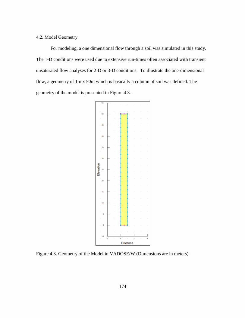
174
4.2. Model Geometry
For modeling, a one dimensional flow through a soil was simulated in this study.
The 1-D conditions were used due to extensive run-times often associated with transient
unsaturated flow analyses for 2-D or 3-D conditions. To illustrate the one-dimensional
flow, a geometry of 1m x 50m which is basically a column of soil was defined. The
geometry of the model is presented in Figure 4.3.
Figure 4.3. Geometry of the Model in VADOSE/W (Dimensions are in meters)
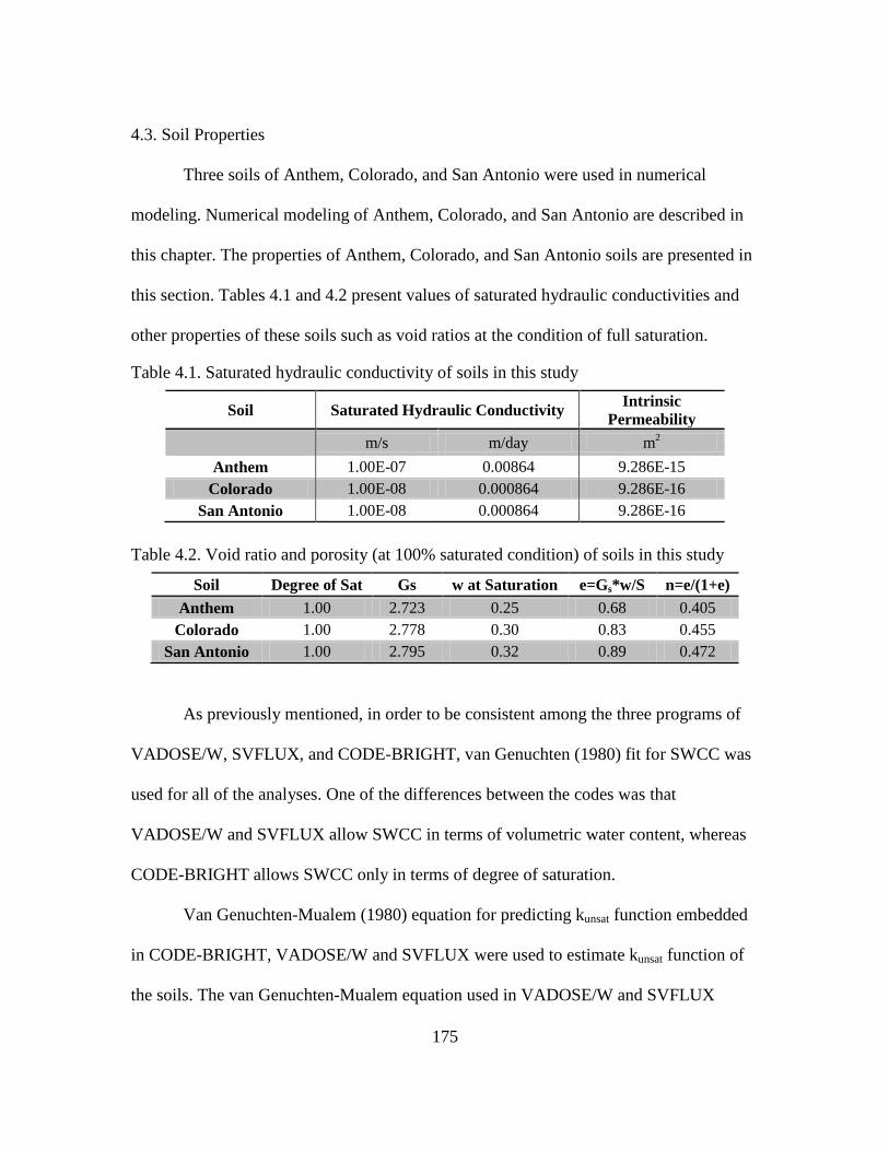
175
4.3. Soil Properties
Three soils of Anthem, Colorado, and San Antonio were used in numerical
modeling. Numerical modeling of Anthem, Colorado, and San Antonio are described in
this chapter. The properties of Anthem, Colorado, and San Antonio soils are presented in
this section. Tables 4.1 and 4.2 present values of saturated hydraulic conductivities and
other properties of these soils such as void ratios at the condition of full saturation.
Table 4.1. Saturated hydraulic conductivity of soils in this study
Soil Saturated Hydraulic Conductivity Intrinsic
Permeability
m/s m/day m
2
Anthem 1.00E-07 0.00864 9.286E-15
Colorado 1.00E-08 0.000864 9.286E-16
San Antonio 1.00E-08 0.000864 9.286E-16
Table 4.2. Void ratio and porosity (at 100% saturated condition) of soils in this study
Soil Degree of Sat Gs w at Saturation e=Gs*w/S n=e/(1+e)
Anthem 1.00 2.723 0.25 0.68 0.405
Colorado 1.00 2.778 0.30 0.83 0.455
San Antonio 1.00 2.795 0.32 0.89 0.472
As previously mentioned, in order to be consistent among the three programs of
VADOSE/W, SVFLUX, and CODE-BRIGHT, van Genuchten (1980) fit for SWCC was
used for all of the analyses. One of the differences between the codes was that
VADOSE/W and SVFLUX allow SWCC in terms of volumetric water content, whereas
CODE-BRIGHT allows SWCC only in terms of degree of saturation.
Van Genuchten-Mualem (1980) equation for predicting kunsat function embedded
in CODE-BRIGHT, VADOSE/W and SVFLUX were used to estimate kunsat function of
the soils. The van Genuchten-Mualem equation used in VADOSE/W and SVFLUX
176
allows van Genuchten SWCC fitting parameters ('a', 'n', and 'm') in terms of volumetric
water content. However, the van Genuchten-Mualem equation that is utilized in CODE-
BRIGHT allows van Genuchten SWCC fitting parameters ('a', 'n', and 'm') in terms of
degree of saturation only. It was established in Chapter 3, that for a given expansive soil,
the SWCC in terms of degree of saturation may have different fitting parameters than the
SWCC in terms of volumetric water content. The van Genuchten-Mualem equation used
in VADOSE/W and SVFLUX uses SWCC in terms of volumetric water content and its
saturated hydraulic conductivity and generates estimation for kunsat function. In CODE-
BRIGHT, however, the Van Genuchten-Mualem equation uses SWCC in terms of degree
of saturation (as opposed to volumetric water content in VADOSE/W and SVFLUX).
Therefore, the kunsat functions generated by VADOSE/W and SVFLUX are the same but
they are different from the kunsat functions generated by CODE-BRIGHT.
It can be seen from all the figures showing kunsat functions (such as Figure 4.6) for
different soils that the values of kunsat are larger for the cases in which SWCC is
corrected for soil volume change (in which case AEV was found to be larger than
uncorrected SWCC). This can be explained by the mechanism of water flow through the
soil. In a saturated soil, all the pore spaces between the solid particles are filled with
water. Once the air-entry value is exceeded (i.e. suctions greater than AEV), air enters the
largest pores and the air-filled pores become non conductive conduits to flow and
increase the tortuosity of the flow path. As a result, the ability of the soil to transport
water (the hydraulic conductivity) decreases (GEO-SLOPE International Ltd., 2012).
Since the SWCC that is corrected for soil volume change generally has a higher AEV
177
(shown in Figures such as 4.5), the desaturation of this soil starts at higher suctions which
means that the decrease in soil hydraulic conductivity occurs at higher suctions. This
leads to larger kunsat values for volume corrected SWCC, on average, compared to the
uncorrected SWCC case. This means that for expansive soils, if the SWCC is corrected
for soil volume change the estimated unsaturated hydraulic conductivity will be larger
compared to the case in which the SWCC is not corrected for soil volume change, and
therefore, water moves faster through the soil with volume corrected SWCC.
SVFLUX and VADOSE/W use van Genuchten-Mualem (1980) equation for
predicting kunsat functions of soils. Van Genuchten (1980) proposed the following closed
form equation to describe the hydraulic conductivity of a soil as a function of matric
suction:
2
21
1
11m
n
mnn
sat
a
aakk
(4.6)
Where:
satk = saturated hydraulic conductivity,
a, n, and m = curve fitting parameters, where n = 1/(1-m), or nnm /1 and
= required suction range.
From the above equations, the hydraulic conductivity function of a soil can be
estimated once the saturated conductivity and the two curve fitting parameters, ‘a’ and
‘m’ (or ‘n’) are known.
178
In CODE-BRIGHT by default, the consistent form of relative hydraulic
conductivity with van Genuchten model-Mualem (1980) is used (Saaltink et al., 2005).
The form of the equation is as below:
2/111
mm
sat SSkk (4.7)
S (degree of saturation) is defined in such a way that ranges between 0 and 1, and
'm' is the van Genuchten parameter for SWCC fit which is the slope of the curve in the
transition zone. The equation used by SVFLUX, VADOSE/W and CODE-BRIGHT for
predicting kunsat function are van Genuchten model-Mualem (1980) and are
interchangeable.
Although all three computer codes use the same van Genuchten model-Mualem
equation (1980) for predicting kunsat function, the kunsat function predicted by CODE-
BRIGHT is different than the ones determined by SVFLUX and VADOSE/W. The
reason for this difference is that the van Genuchten model-Mualem (1980) equation in
SVFLUX and VADOSE/W uses van Genuchten parameter (‘a’, ‘n’, and ‘m’) that
correspond to SWCC in terms of volumetric water content. However, the van Genuchten
model-Mualem (1980) equation in CODE-BRIGHT uses S (degree of saturation) and ‘m’
parameter of SWCC in terms of degree of saturation. As it was established earlier, for a
given soil that exhibits volume change, the van Genuchten parameters of SWCC in terms
of volumetric water content may be different that the van Genuchten parameters of
SWCC in terms of degree of saturation. This difference in van Genuchten parameters
leads to differences in estimated kunsat function.
179
4.3.1. Anthem Soil
Figures 4.4 and 4.5 show the SWCC of Anthem soil in terms of volumetric
moisture content and degree of saturation. The data points shown in these figures were
obtained from laboratory tests described in Chapter 3. Shown in these figures are also the
van Genuchten (1980) fits to the SWCC data points. It can be seen that for both SWCC's
(in terms of volumetric water content and degree of saturation) the "a" parameter (which
corresponds to AEV) is higher for the corrected curve.
Figure 4.6 shows hydraulic conductivity versus suction, otherwise known as kunsat
function for Anthem soil found by van Genuchten-Mualem (1980) embedded in
SVFLUX and CODE-BRIGHT. It can be seen that for any given suction, the kunsat
generated by either SVFLUX or CODE-BRIGHT is higher for corrected curve compared
to the uncorrected curve.
It was also found that for Anthem soil the kunsat values estimated by CODE-
BRIGHT are generally smaller than the kunsat values estimated by SVFLUX. This is due
to the difference in the equation used for estimating the kunsat function. Therefore, it
generally takes longer for the model in CODE-BRIGHT to reach equilibrium compared
to the same model in SVFLUX. In other words, the rate of changes in suction (e.g.
progression of wetted front) is larger for corrected SWCC compared to uncorrected case.
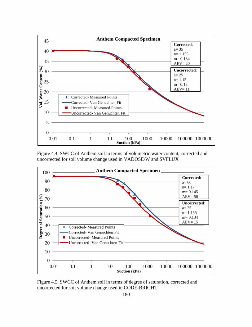
180
Figure 4.4. SWCC of Anthem soil in terms of volumetric water content, corrected and
uncorrected for soil volume change used in VADOSE/W and SVFLUX
Figure 4.5. SWCC of Anthem soil in terms of degree of saturation, corrected and
uncorrected for soil volume change used in CODE-BRIGHT
0
5
10
15
20
25
30
35
40
45
0.01 0.1 1 10 100 1000 10000 100000 1000000
Vo
l. W
ate
r C
on
ten
t (%
)
Suction (kPa)
Anthem Compacted Specimen
Corrected- Measured Points
Corrected- Van Genuchten Fit
Uncorrected- Measured Points
Uncorrected- Van Genuchten Fit
Corrected:
a= 35
n= 1.155
m= 0.134
AEV= 20
Uncorrected:
a= 25
n= 1.15
m= 0.13
AEV= 11
0
10
20
30
40
50
60
70
80
90
100
0.01 0.1 1 10 100 1000 10000 100000 1000000
Deg
ree
of
Sa
tura
tio
n (
%)
Suction (kPa)
Anthem Compacted Specimen
Corrected- Measured Points
Corrected- Van Genuchten Fit
Uncorrected- Measured Points
Uncorrected- Van Genuchten Fit
Corrected:
a= 60
n= 1.17
m= 0.145
AEV= 50
Uncorrected:
a= 25
n= 1.155
m= 0.134
AEV= 15
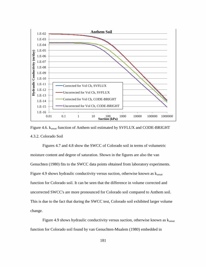
181
Figure 4.6. kunsat function of Anthem soil estimated by SVFLUX and CODE-BRIGHT
4.3.2. Colorado Soil
Figures 4.7 and 4.8 show the SWCC of Colorado soil in terms of volumetric
moisture content and degree of saturation. Shown in the figures are also the van
Genuchten (1980) fits to the SWCC data points obtained from laboratory experiments.
Figure 4.9 shows hydraulic conductivity versus suction, otherwise known as kunsat
function for Colorado soil. It can be seen that the difference in volume corrected and
uncorrected SWCC's are more pronounced for Colorado soil compared to Anthem soil.
This is due to the fact that during the SWCC test, Colorado soil exhibited larger volume
change.
Figure 4.9 shows hydraulic conductivity versus suction, otherwise known as kunsat
function for Colorado soil found by van Genuchten-Mualem (1980) embedded in
1.E-16
1.E-15
1.E-14
1.E-13
1.E-12
1.E-11
1.E-10
1.E-09
1.E-08
1.E-07
1.E-06
1.E-05
1.E-04
1.E-03
1.E-02
0.01 0.1 1 10 100 1000 10000 100000 1000000
Hy
dra
uli
c C
on
du
ctiv
ity
(m
/da
y)
Suction (kPa)
Anthem Soil
Corrected for Vol Ch, SVFLUX
Uncorrected for Vol Ch, SVFLUX
Corrected for Vol Ch, CODE-BRIGHT
Uncorrected for Vol Ch, CODE-BRIGHT
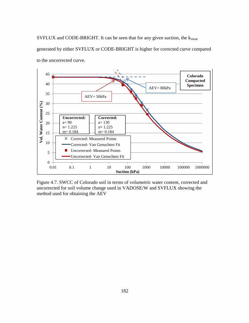
182
SVFLUX and CODE-BRIGHT. It can be seen that for any given suction, the kunsat
generated by either SVFLUX or CODE-BRIGHT is higher for corrected curve compared
to the uncorrected curve.
Figure 4.7. SWCC of Colorado soil in terms of volumetric water content, corrected and
uncorrected for soil volume change used in VADOSE/W and SVFLUX showing the
method used for obtaining the AEV
0
5
10
15
20
25
30
35
40
45
0.01 0.1 1 10 100 1000 10000 100000 1000000
Vo
l. W
ate
r C
on
ten
t (%
)
Suction (kPa)
Corrected- Measured Points
Corrected- Van Genuchten Fit
Uncorrected- Measured Points
Uncorrected- Van Genuchten Fit
Corrected:
a= 130
n= 1.225
m= 0.184
Uncorrected:
a= 90
n= 1.225
m= 0.184
AEV= 80kPa
AEV= 50kPa
Colorado
Compacted
Specimen
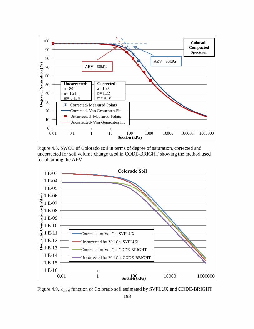
183
Figure 4.8. SWCC of Colorado soil in terms of degree of saturation, corrected and
uncorrected for soil volume change used in CODE-BRIGHT showing the method used
for obtaining the AEV
Figure 4.9. kunsat function of Colorado soil estimated by SVFLUX and CODE-BRIGHT
0
10
20
30
40
50
60
70
80
90
100
0.01 0.1 1 10 100 1000 10000 100000 1000000
Deg
ree
of
Sa
tura
tio
n (
%)
Suction (kPa)
Corrected- Measured Points
Corrected- Van Genuchten Fit
Uncorrected- Measured Points
Uncorrected- Van Genuchten Fit
Corrected:
a= 150
n= 1.22
m= 0.18
Uncorrected:
a= 80
n= 1.21
m= 0.174
AEV= 90kPa
AEV= 60kPa
Colorado
Compacted
Specimen
1.E-16
1.E-15
1.E-14
1.E-13
1.E-12
1.E-11
1.E-10
1.E-09
1.E-08
1.E-07
1.E-06
1.E-05
1.E-04
1.E-03
0.01 1 100 10000 1000000
Hy
dra
uli
c C
on
du
ctiv
ity
(m
/da
y)
Suction (kPa)
Colorado Soil
Corrected for Vol Ch, SVFLUX
Uncorrected for Vol Ch, SVFLUX
Corrected for Vol Ch, CODE-BRIGHT
Uncorrected for Vol Ch, CODE-BRIGHT
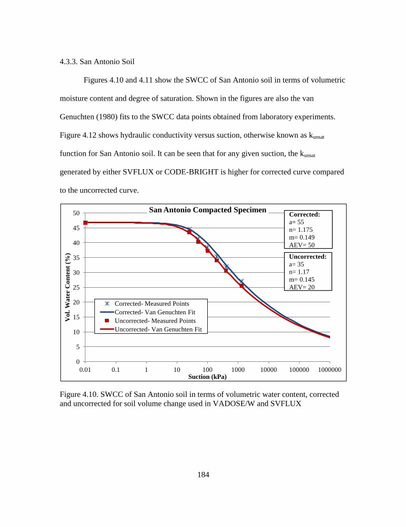
184
4.3.3. San Antonio Soil
Figures 4.10 and 4.11 show the SWCC of San Antonio soil in terms of volumetric
moisture content and degree of saturation. Shown in the figures are also the van
Genuchten (1980) fits to the SWCC data points obtained from laboratory experiments.
Figure 4.12 shows hydraulic conductivity versus suction, otherwise known as kunsat
function for San Antonio soil. It can be seen that for any given suction, the kunsat
generated by either SVFLUX or CODE-BRIGHT is higher for corrected curve compared
to the uncorrected curve.
Figure 4.10. SWCC of San Antonio soil in terms of volumetric water content, corrected
and uncorrected for soil volume change used in VADOSE/W and SVFLUX
0
5
10
15
20
25
30
35
40
45
50
0.01 0.1 1 10 100 1000 10000 100000 1000000
Vo
l. W
ate
r C
on
ten
t (%
)
Suction (kPa)
San Antonio Compacted Specimen
Corrected- Measured Points
Corrected- Van Genuchten Fit
Uncorrected- Measured Points
Uncorrected- Van Genuchten Fit
Corrected:
a= 55
n= 1.175
m= 0.149
AEV= 50
Uncorrected:
a= 35
n= 1.17
m= 0.145
AEV= 20
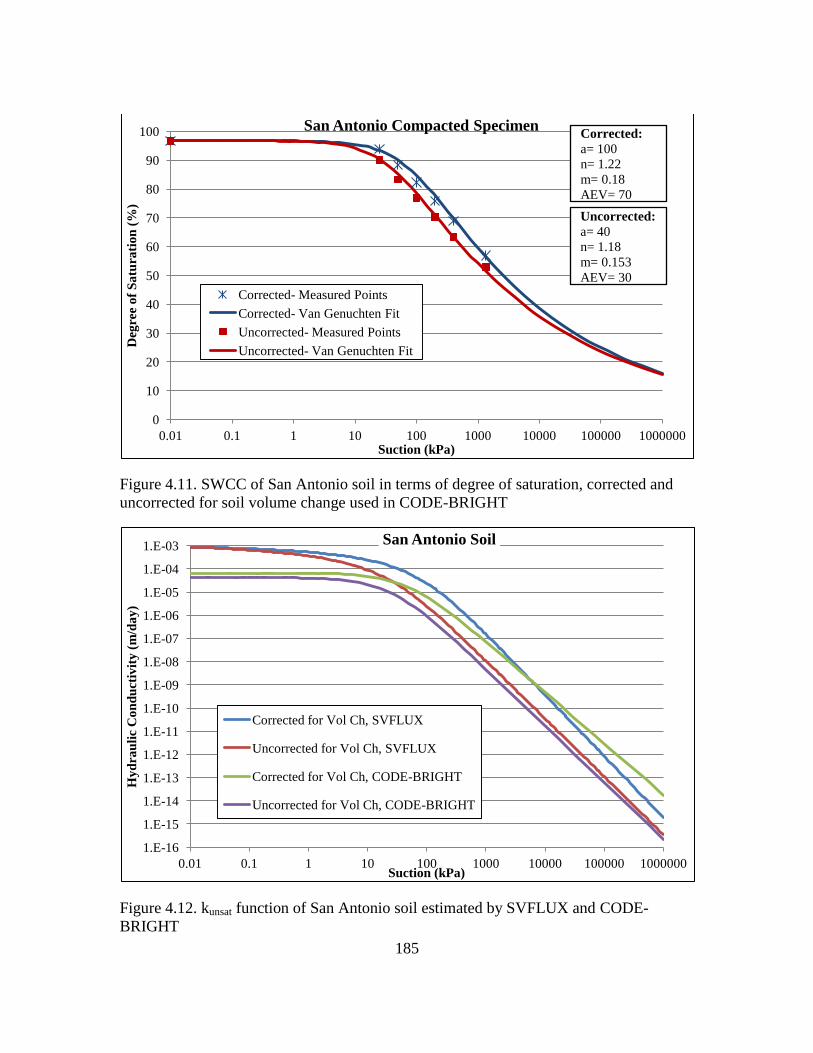
185
Figure 4.11. SWCC of San Antonio soil in terms of degree of saturation, corrected and
uncorrected for soil volume change used in CODE-BRIGHT
Figure 4.12. kunsat function of San Antonio soil estimated by SVFLUX and CODE-
BRIGHT
0
10
20
30
40
50
60
70
80
90
100
0.01 0.1 1 10 100 1000 10000 100000 1000000
Deg
ree
of
Sa
tura
tio
n (
%)
Suction (kPa)
San Antonio Compacted Specimen
Corrected- Measured Points
Corrected- Van Genuchten Fit
Uncorrected- Measured Points
Uncorrected- Van Genuchten Fit
Corrected:
a= 100
n= 1.22
m= 0.18
AEV= 70
Uncorrected:
a= 40
n= 1.18
m= 0.153
AEV= 30
1.E-16
1.E-15
1.E-14
1.E-13
1.E-12
1.E-11
1.E-10
1.E-09
1.E-08
1.E-07
1.E-06
1.E-05
1.E-04
1.E-03
0.01 0.1 1 10 100 1000 10000 100000 1000000
Hy
dra
uli
c C
on
du
ctiv
ity
(m
/da
y)
Suction (kPa)
San Antonio Soil
Corrected for Vol Ch, SVFLUX
Uncorrected for Vol Ch, SVFLUX
Corrected for Vol Ch, CODE-BRIGHT
Uncorrected for Vol Ch, CODE-BRIGHT
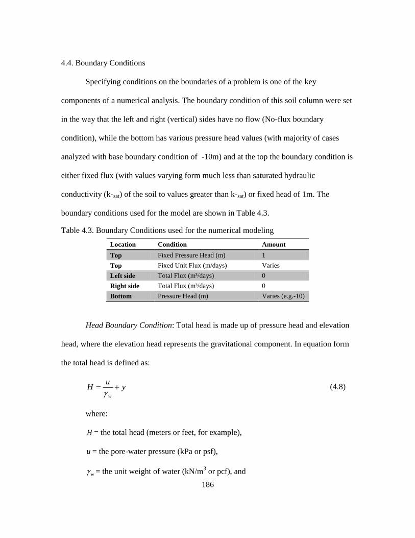
186
4.4. Boundary Conditions
Specifying conditions on the boundaries of a problem is one of the key
components of a numerical analysis. The boundary condition of this soil column were set
in the way that the left and right (vertical) sides have no flow (No-flux boundary
condition), while the bottom has various pressure head values (with majority of cases
analyzed with base boundary condition of -10m) and at the top the boundary condition is
either fixed flux (with values varying form much less than saturated hydraulic
conductivity (k-sat) of the soil to values greater than k-sat) or fixed head of 1m. The
boundary conditions used for the model are shown in Table 4.3.
Table 4.3. Boundary Conditions used for the numerical modeling
Location Condition Amount
Top Fixed Pressure Head (m) 1
Top Fixed Unit Flux (m/days) Varies
Left side Total Flux (m³/days) 0
Right side Total Flux (m³/days) 0
Bottom Pressure Head (m) Varies (e.g.-10)
Head Boundary Condition: Total head is made up of pressure head and elevation
head, where the elevation head represents the gravitational component. In equation form
the total head is defined as:
yu
Hw
(4.8)
where:
H = the total head (meters or feet, for example),
u = the pore-water pressure (kPa or psf),
w = the unit weight of water (kN/m3 or pcf), and
187
y = the elevation (meters or feet).
The term w
u
is referred to as pressure head (represented in units of length). For
the cases of the simulation with fixed pressure head at the top of the soil column in this
study, the quantity of this pressure head is 1m. This can represent a ponding condition at
the surface of the soil.
Flux Boundary Condition: The second type of boundary conditions used in this
study was a fixed rate of flow across the edge of an element. An example may be the rate
of infiltration or application of precipitation. This is often referred to as a flux boundary.
Different values of fixed flux boundary conditions at the top of the soil column were
used, some of the fixed flux values were smaller than ksat, and some were greater. The
results were then compared against one another. For the cases in which the top boundary
condition was fixed flux with flux values smaller than ksat, the soil column gets wet but
since the flux is not big enough, the water pressure throughout the soil does not become
positive. In other words, there is suction within the entire soil profile (at the steady-state
condition). If the value of top fixed flux is equal to ksat the soil gets wet and the suction
for the majority of the soil profile ends up near zero. If the value of top fixed flux is
larger than ksat, the soil gets wet and the final (i.e. steady-state) condition shows positive
water pressure within the profile. It should noticed that since the bottom boundary
condition is set to negative water pressure values (e.g. -100kPa or pressure head of -
10m), the bottom part of the soil column will have suction (negative water pressure) for
all of the cases.
188
4.5. VADOSE/W
One of the computer codes used for the numerical modeling in this study was
VADOSE/W. VADOSE/W is a commercial software that is being used by numerous
practitioners to model fluid flow through soils. VADOSE/W is a finite element program
that can be used to model movement and distribution of pore water within porous
materials such as soil and bedrock. VADOSE/W can model both saturated and
unsaturated flow.
In VADOSE/W for an unsaturated flow analysis the finite element equation prior
to solving for the unknowns is (Geo-Slope International, 2012):
[K]{H} = {Q} (4.9)
Where:
[K] = a matrix of coefficients related to geometry and materials properties (global
property matrix),
{H} = a vector of the total hydraulic heads at the nodes, and
{Q} = a vector of the flow quantities at the node.
The objective is to solve for the primary unknowns, which in an unsaturated flow
analysis are the total hydraulic head at each node (Geo-Slope International, 2012). The
specified H or Q values are the boundary conditions. It should be mentioned that
specified head boundary conditions can be converted into nodal Q values. When H is
specified, the solution to the finite element Equation 4.9 above will provide Q.
Alternatively, when Q is specified, the solution will provide H. The equation always
needs to be in balance. So when an H is specified at a node, the computed Q is the Q that
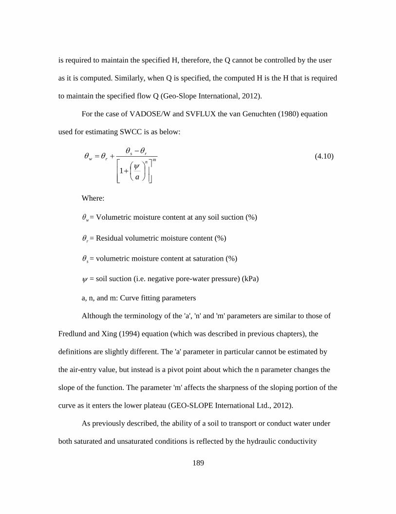
189
is required to maintain the specified H, therefore, the Q cannot be controlled by the user
as it is computed. Similarly, when Q is specified, the computed H is the H that is required
to maintain the specified flow Q (Geo-Slope International, 2012).
For the case of VADOSE/W and SVFLUX the van Genuchten (1980) equation
used for estimating SWCC is as below:
m
n
rs
rw
a
1
(4.10)
Where:
w = Volumetric moisture content at any soil suction (%)
r = Residual volumetric moisture content (%)
s = volumetric moisture content at saturation (%)
= soil suction (i.e. negative pore-water pressure) (kPa)
a, n, and m: Curve fitting parameters
Although the terminology of the 'a', 'n' and 'm' parameters are similar to those of
Fredlund and Xing (1994) equation (which was described in previous chapters), the
definitions are slightly different. The 'a' parameter in particular cannot be estimated by
the air-entry value, but instead is a pivot point about which the n parameter changes the
slope of the function. The parameter 'm' affects the sharpness of the sloping portion of the
curve as it enters the lower plateau (GEO-SLOPE International Ltd., 2012).
As previously described, the ability of a soil to transport or conduct water under
both saturated and unsaturated conditions is reflected by the hydraulic conductivity
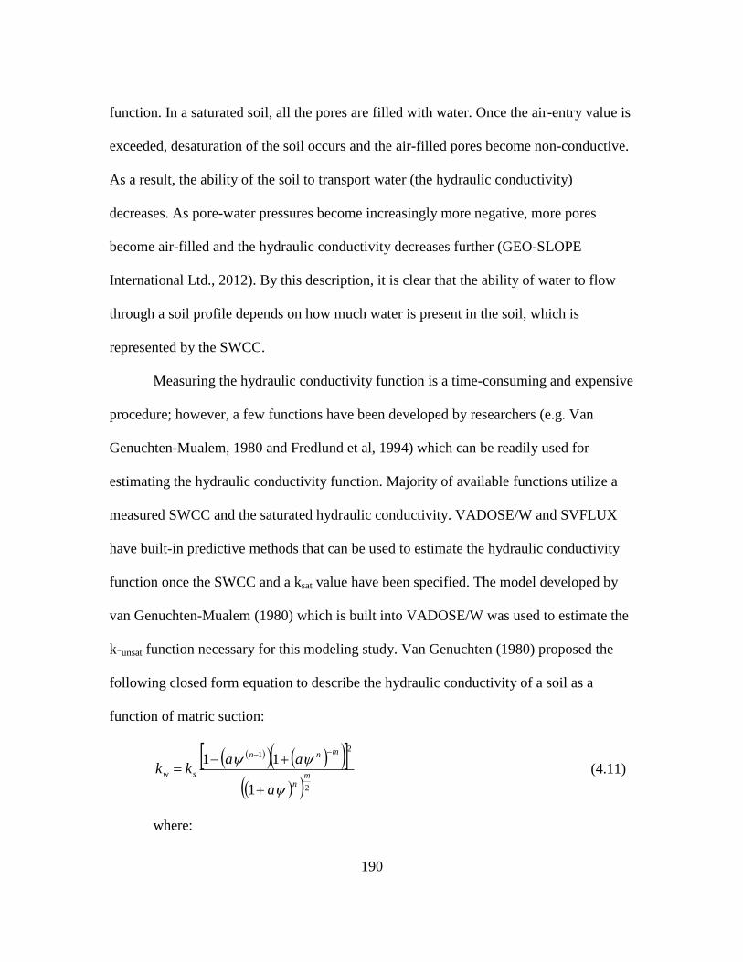
190
function. In a saturated soil, all the pores are filled with water. Once the air-entry value is
exceeded, desaturation of the soil occurs and the air-filled pores become non-conductive.
As a result, the ability of the soil to transport water (the hydraulic conductivity)
decreases. As pore-water pressures become increasingly more negative, more pores
become air-filled and the hydraulic conductivity decreases further (GEO-SLOPE
International Ltd., 2012). By this description, it is clear that the ability of water to flow
through a soil profile depends on how much water is present in the soil, which is
represented by the SWCC.
Measuring the hydraulic conductivity function is a time-consuming and expensive
procedure; however, a few functions have been developed by researchers (e.g. Van
Genuchten-Mualem, 1980 and Fredlund et al, 1994) which can be readily used for
estimating the hydraulic conductivity function. Majority of available functions utilize a
measured SWCC and the saturated hydraulic conductivity. VADOSE/W and SVFLUX
have built-in predictive methods that can be used to estimate the hydraulic conductivity
function once the SWCC and a ksat value have been specified. The model developed by
van Genuchten-Mualem (1980) which is built into VADOSE/W was used to estimate the
k-unsat function necessary for this modeling study. Van Genuchten (1980) proposed the
following closed form equation to describe the hydraulic conductivity of a soil as a
function of matric suction:
2
21
1
11m
n
mnn
sw
a
aakk
(4.11)
where:
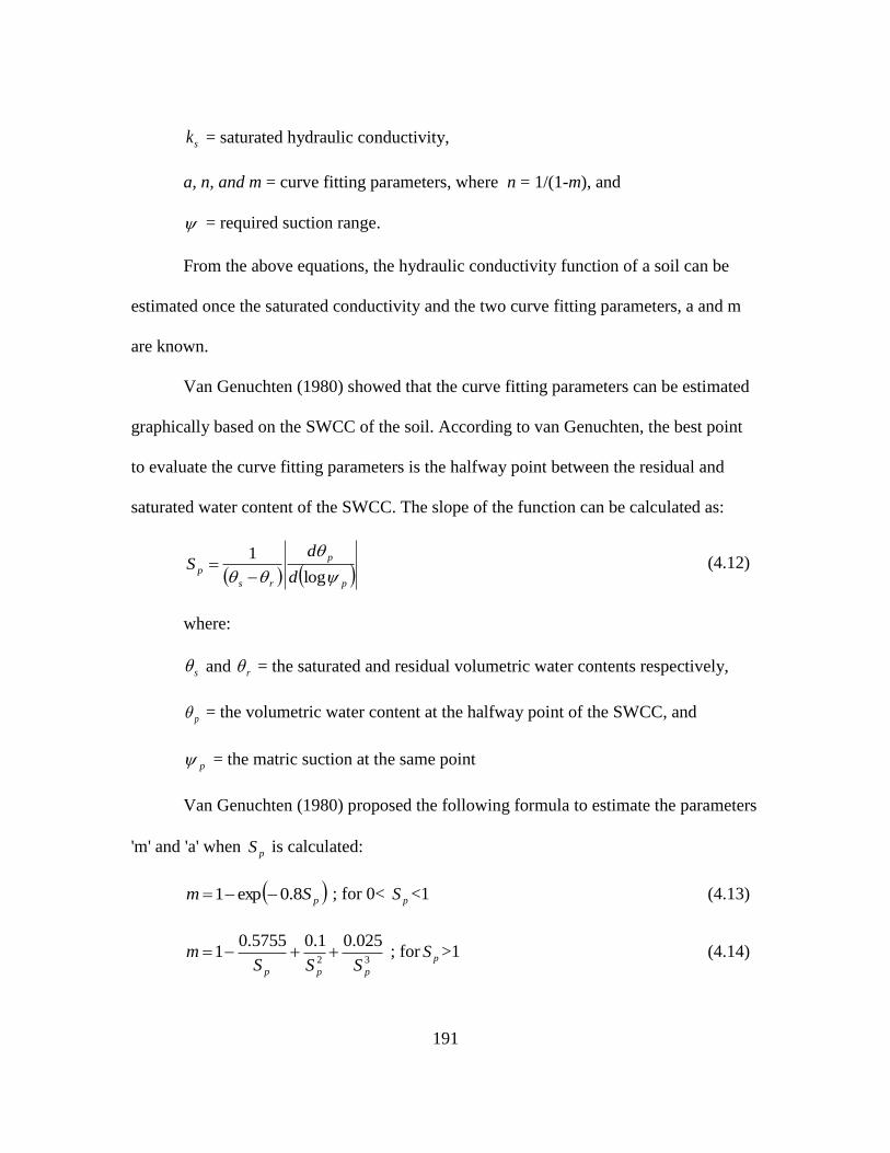
191
sk = saturated hydraulic conductivity,
a, n, and m = curve fitting parameters, where n = 1/(1-m), and
= required suction range.
From the above equations, the hydraulic conductivity function of a soil can be
estimated once the saturated conductivity and the two curve fitting parameters, a and m
are known.
Van Genuchten (1980) showed that the curve fitting parameters can be estimated
graphically based on the SWCC of the soil. According to van Genuchten, the best point
to evaluate the curve fitting parameters is the halfway point between the residual and
saturated water content of the SWCC. The slope of the function can be calculated as:
p
p
rs
pd
dS
log
1
(4.12)
where:
s and r = the saturated and residual volumetric water contents respectively,
p = the volumetric water content at the halfway point of the SWCC, and
p = the matric suction at the same point
Van Genuchten (1980) proposed the following formula to estimate the parameters
'm' and 'a' when pS is calculated:
pSm 8.0exp1 ; for 0< pS <1 (4.13)
32
025.01.05755.01
ppp SSSm ; for pS >1 (4.14)
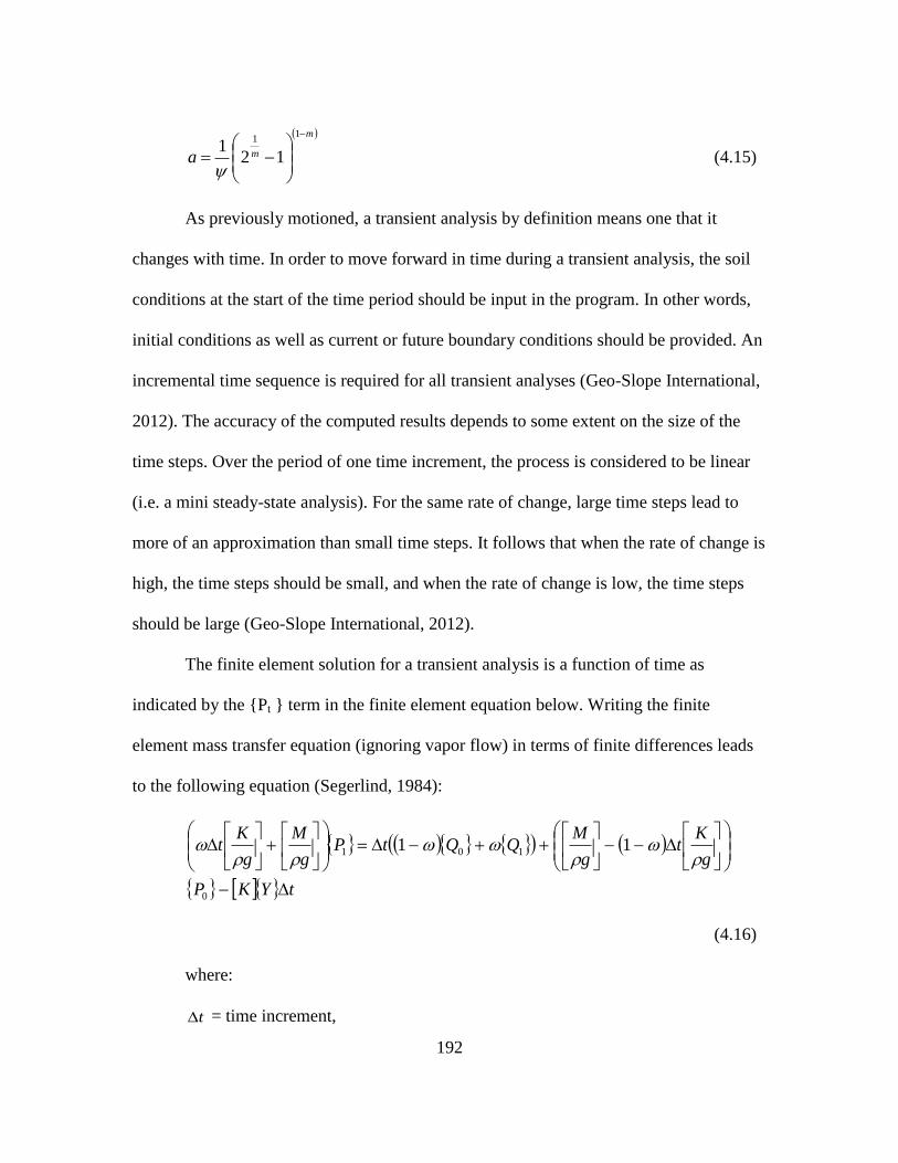
192
m
ma
11
121
(4.15)
As previously motioned, a transient analysis by definition means one that it
changes with time. In order to move forward in time during a transient analysis, the soil
conditions at the start of the time period should be input in the program. In other words,
initial conditions as well as current or future boundary conditions should be provided. An
incremental time sequence is required for all transient analyses (Geo-Slope International,
2012). The accuracy of the computed results depends to some extent on the size of the
time steps. Over the period of one time increment, the process is considered to be linear
(i.e. a mini steady-state analysis). For the same rate of change, large time steps lead to
more of an approximation than small time steps. It follows that when the rate of change is
high, the time steps should be small, and when the rate of change is low, the time steps
should be large (Geo-Slope International, 2012).
The finite element solution for a transient analysis is a function of time as
indicated by the {Pt } term in the finite element equation below. Writing the finite
element mass transfer equation (ignoring vapor flow) in terms of finite differences leads
to the following equation (Segerlind, 1984):
tYKP
g
Kt
g
MQQtP
g
M
g
Kt
0
101 11
(4.16)
where:
t = time increment,
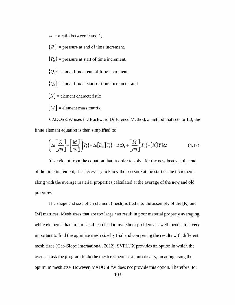
193
= a ratio between 0 and 1,
1P = pressure at end of time increment,
0P = pressure at start of time increment,
1Q = nodal flux at end of time increment,
0Q = nodal flux at start of time increment, and
K = element characteristic
M = element mass matrix
VADOSE/W uses the Backward Difference Method, a method that sets to 1.0, the
finite element equation is then simplified to:
tYKPg
MtQTDtP
g
M
g
Kt
01121
(4.17)
It is evident from the equation that in order to solve for the new heads at the end
of the time increment, it is necessary to know the pressure at the start of the increment,
along with the average material properties calculated at the average of the new and old
pressures.
The shape and size of an element (mesh) is tied into the assembly of the [K] and
[M] matrices. Mesh sizes that are too large can result in poor material property averaging,
while elements that are too small can lead to overshoot problems as well, hence, it is very
important to find the optimize mesh size by trial and comparing the results with different
mesh sizes (Geo-Slope International, 2012). SVFLUX provides an option in which the
user can ask the program to do the mesh refinement automatically, meaning using the
optimum mesh size. However, VADOSE/W does not provide this option. Therefore, for
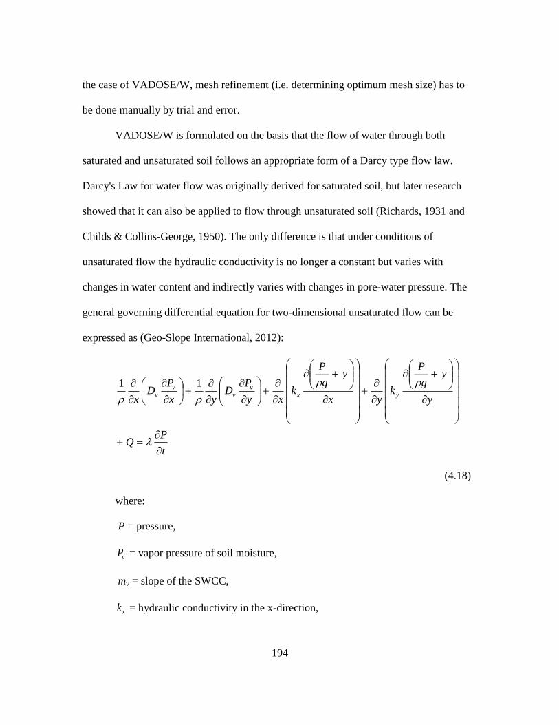
194
the case of VADOSE/W, mesh refinement (i.e. determining optimum mesh size) has to
be done manually by trial and error.
VADOSE/W is formulated on the basis that the flow of water through both
saturated and unsaturated soil follows an appropriate form of a Darcy type flow law.
Darcy's Law for water flow was originally derived for saturated soil, but later research
showed that it can also be applied to flow through unsaturated soil (Richards, 1931 and
Childs & Collins-George, 1950). The only difference is that under conditions of
unsaturated flow the hydraulic conductivity is no longer a constant but varies with
changes in water content and indirectly varies with changes in pore-water pressure. The
general governing differential equation for two-dimensional unsaturated flow can be
expressed as (Geo-Slope International, 2012):
t
PQ
y
yg
P
kyx
yg
P
kxy
PD
yx
PD
xyx
v
v
v
v
11
(4.18)
where:
P = pressure,
vP = vapor pressure of soil moisture,
mv = slope of the SWCC,
xk = hydraulic conductivity in the x-direction,
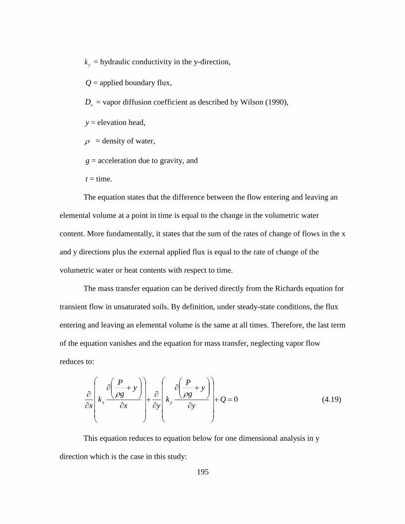
195
yk = hydraulic conductivity in the y-direction,
Q = applied boundary flux,
vD = vapor diffusion coefficient as described by Wilson (1990),
y = elevation head,
= density of water,
g = acceleration due to gravity, and
t = time.
The equation states that the difference between the flow entering and leaving an
elemental volume at a point in time is equal to the change in the volumetric water
content. More fundamentally, it states that the sum of the rates of change of flows in the x
and y directions plus the external applied flux is equal to the rate of change of the
volumetric water or heat contents with respect to time.
The mass transfer equation can be derived directly from the Richards equation for
transient flow in unsaturated soils. By definition, under steady-state conditions, the flux
entering and leaving an elemental volume is the same at all times. Therefore, the last term
of the equation vanishes and the equation for mass transfer, neglecting vapor flow
reduces to:
0
Q
y
yg
P
kyx
yg
P
kx
yx
(4.19)
This equation reduces to equation below for one dimensional analysis in y
direction which is the case in this study:
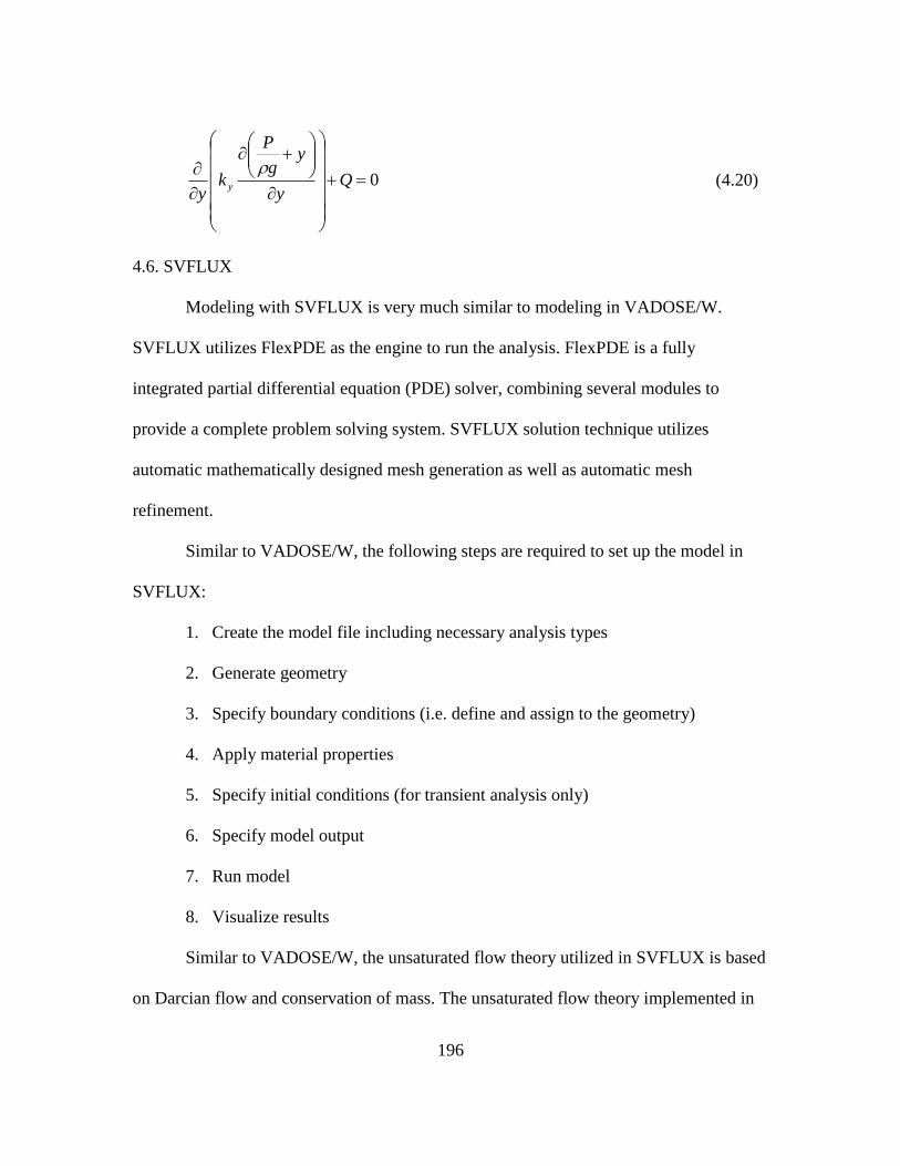
196
0
Q
y
yg
P
ky
y
(4.20)
4.6. SVFLUX
Modeling with SVFLUX is very much similar to modeling in VADOSE/W.
SVFLUX utilizes FlexPDE as the engine to run the analysis. FlexPDE is a fully
integrated partial differential equation (PDE) solver, combining several modules to
provide a complete problem solving system. SVFLUX solution technique utilizes
automatic mathematically designed mesh generation as well as automatic mesh
refinement.
Similar to VADOSE/W, the following steps are required to set up the model in
SVFLUX:
1. Create the model file including necessary analysis types
2. Generate geometry
3. Specify boundary conditions (i.e. define and assign to the geometry)
4. Apply material properties
5. Specify initial conditions (for transient analysis only)
6. Specify model output
7. Run model
8. Visualize results
Similar to VADOSE/W, the unsaturated flow theory utilized in SVFLUX is based
on Darcian flow and conservation of mass. The unsaturated flow theory implemented in
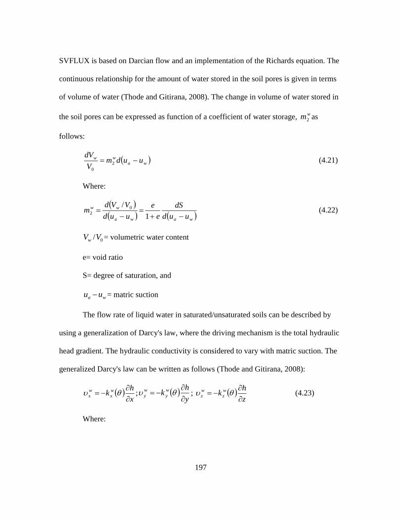
197
SVFLUX is based on Darcian flow and an implementation of the Richards equation. The
continuous relationship for the amount of water stored in the soil pores is given in terms
of volume of water (Thode and Gitirana, 2008). The change in volume of water stored in
the soil pores can be expressed as function of a coefficient of water storage, wm2 as
follows:
wa
ww uudmV
dV 2
0
(4.21)
Where:
wawa
ww
uud
dS
e
e
uud
VVdm
1
/ 0
2 (4.22)
0/VVw = volumetric water content
e= void ratio
S= degree of saturation, and
wa uu = matric suction
The flow rate of liquid water in saturated/unsaturated soils can be described by
using a generalization of Darcy's law, where the driving mechanism is the total hydraulic
head gradient. The hydraulic conductivity is considered to vary with matric suction. The
generalized Darcy's law can be written as follows (Thode and Gitirana, 2008):
x
hk w
x
w
x
;
y
hk w
y
w
y
;
z
hk w
z
w
z
(4.23)
Where:
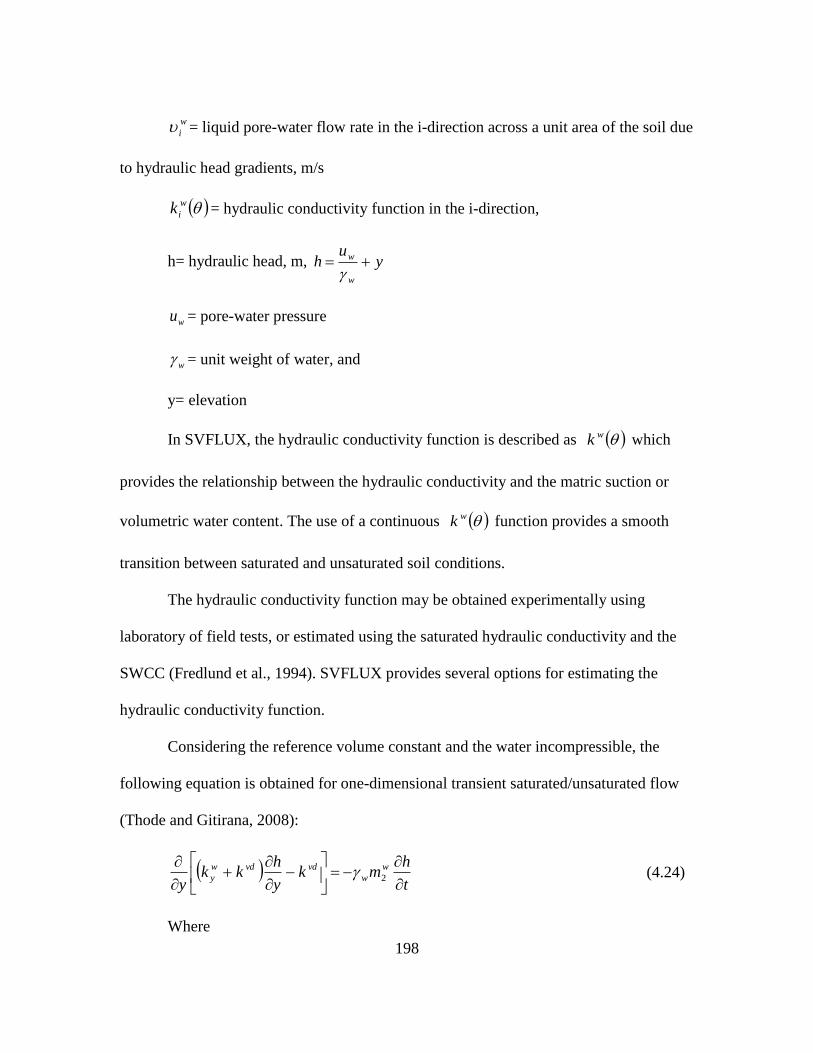
198
w
i = liquid pore-water flow rate in the i-direction across a unit area of the soil due
to hydraulic head gradients, m/s
w
ik = hydraulic conductivity function in the i-direction,
h= hydraulic head, m, yu
hw
w
wu = pore-water pressure
w = unit weight of water, and
y= elevation
In SVFLUX, the hydraulic conductivity function is described as wk which
provides the relationship between the hydraulic conductivity and the matric suction or
volumetric water content. The use of a continuous wk function provides a smooth
transition between saturated and unsaturated soil conditions.
The hydraulic conductivity function may be obtained experimentally using
laboratory of field tests, or estimated using the saturated hydraulic conductivity and the
SWCC (Fredlund et al., 1994). SVFLUX provides several options for estimating the
hydraulic conductivity function.
Considering the reference volume constant and the water incompressible, the
following equation is obtained for one-dimensional transient saturated/unsaturated flow
(Thode and Gitirana, 2008):
t
hmk
y
hkk
y
w
w
vdvdw
y
2 (4.24)
Where
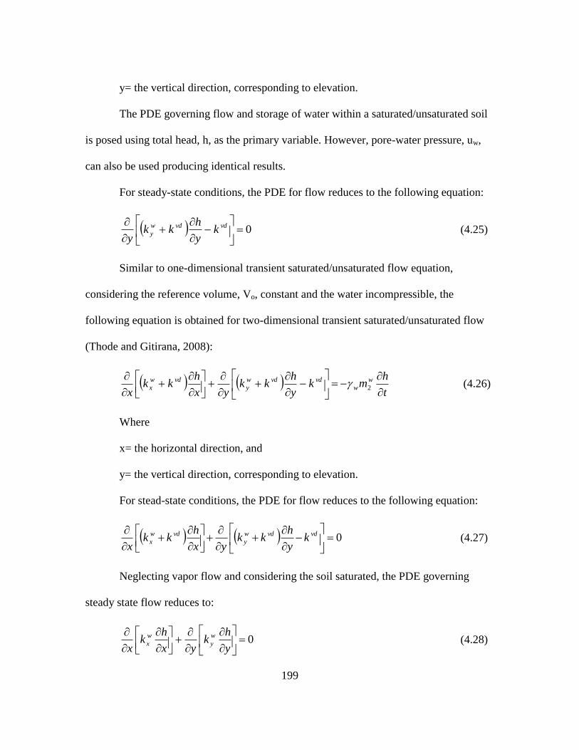
199
y= the vertical direction, corresponding to elevation.
The PDE governing flow and storage of water within a saturated/unsaturated soil
is posed using total head, h, as the primary variable. However, pore-water pressure, uw,
can also be used producing identical results.
For steady-state conditions, the PDE for flow reduces to the following equation:
0
vdvdw
y ky
hkk
y (4.25)
Similar to one-dimensional transient saturated/unsaturated flow equation,
considering the reference volume, Vo, constant and the water incompressible, the
following equation is obtained for two-dimensional transient saturated/unsaturated flow
(Thode and Gitirana, 2008):
t
hmk
y
hkk
yx
hkk
x
w
w
vdvdw
y
vdw
x
2 (4.26)
Where
x= the horizontal direction, and
y= the vertical direction, corresponding to elevation.
For stead-state conditions, the PDE for flow reduces to the following equation:
0
vdvdw
y
vdw
x ky
hkk
yx
hkk
x (4.27)
Neglecting vapor flow and considering the soil saturated, the PDE governing
steady state flow reduces to:
0
y
hk
yx
hk
x
w
y
w
x (4.28)
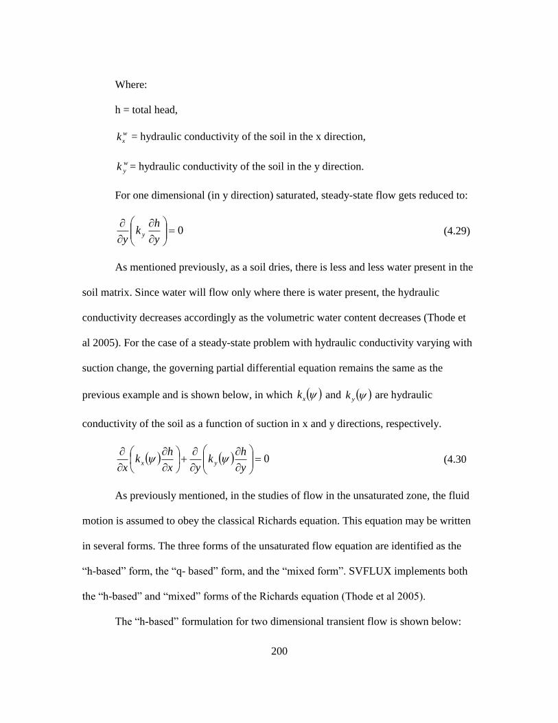
200
Where:
h = total head,
w
xk = hydraulic conductivity of the soil in the x direction,
w
yk = hydraulic conductivity of the soil in the y direction.
For one dimensional (in y direction) saturated, steady-state flow gets reduced to:
0
y
hk
yy (4.29)
As mentioned previously, as a soil dries, there is less and less water present in the
soil matrix. Since water will flow only where there is water present, the hydraulic
conductivity decreases accordingly as the volumetric water content decreases (Thode et
al 2005). For the case of a steady-state problem with hydraulic conductivity varying with
suction change, the governing partial differential equation remains the same as the
previous example and is shown below, in which xk and yk are hydraulic
conductivity of the soil as a function of suction in x and y directions, respectively.
0
y
hk
yx
hk
xyx (4.30
As previously mentioned, in the studies of flow in the unsaturated zone, the fluid
motion is assumed to obey the classical Richards equation. This equation may be written
in several forms. The three forms of the unsaturated flow equation are identified as the
“h-based” form, the “q- based” form, and the “mixed form”. SVFLUX implements both
the “h-based” and “mixed” forms of the Richards equation (Thode et al 2005).
The “h-based” formulation for two dimensional transient flow is shown below:
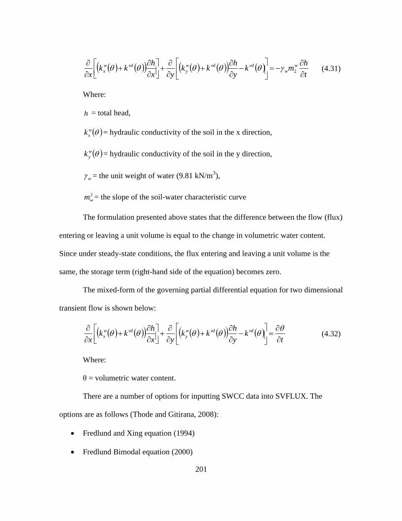
201
t
hmk
y
hkk
yx
hkk
x
w
w
vdvdw
y
vdw
x
2 (4.31)
Where:
h = total head,
w
xk = hydraulic conductivity of the soil in the x direction,
w
yk = hydraulic conductivity of the soil in the y direction,
w = the unit weight of water (9.81 kN/m3),
2
wm = the slope of the soil-water characteristic curve
The formulation presented above states that the difference between the flow (flux)
entering or leaving a unit volume is equal to the change in volumetric water content.
Since under steady-state conditions, the flux entering and leaving a unit volume is the
same, the storage term (right-hand side of the equation) becomes zero.
The mixed-form of the governing partial differential equation for two dimensional
transient flow is shown below:
t
ky
hkk
yx
hkk
x
vdvdw
y
vdw
x
(4.32)
Where:
θ = volumetric water content.
There are a number of options for inputting SWCC data into SVFLUX. The
options are as follows (Thode and Gitirana, 2008):
Fredlund and Xing equation (1994)
Fredlund Bimodal equation (2000)
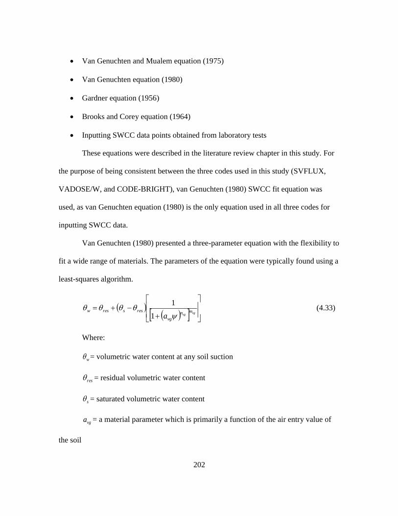
202
Van Genuchten and Mualem equation (1975)
Van Genuchten equation (1980)
Gardner equation (1956)
Brooks and Corey equation (1964)
Inputting SWCC data points obtained from laboratory tests
These equations were described in the literature review chapter in this study. For
the purpose of being consistent between the three codes used in this study (SVFLUX,
VADOSE/W, and CODE-BRIGHT), van Genuchten (1980) SWCC fit equation was
used, as van Genuchten equation (1980) is the only equation used in all three codes for
inputting SWCC data.
Van Genuchten (1980) presented a three-parameter equation with the flexibility to
fit a wide range of materials. The parameters of the equation were typically found using a
least-squares algorithm.
vgvg
mn
vg
ressresw
a
1
1 (4.33)
Where:
w = volumetric water content at any soil suction
res = residual volumetric water content
s = saturated volumetric water content
vga = a material parameter which is primarily a function of the air entry value of
the soil
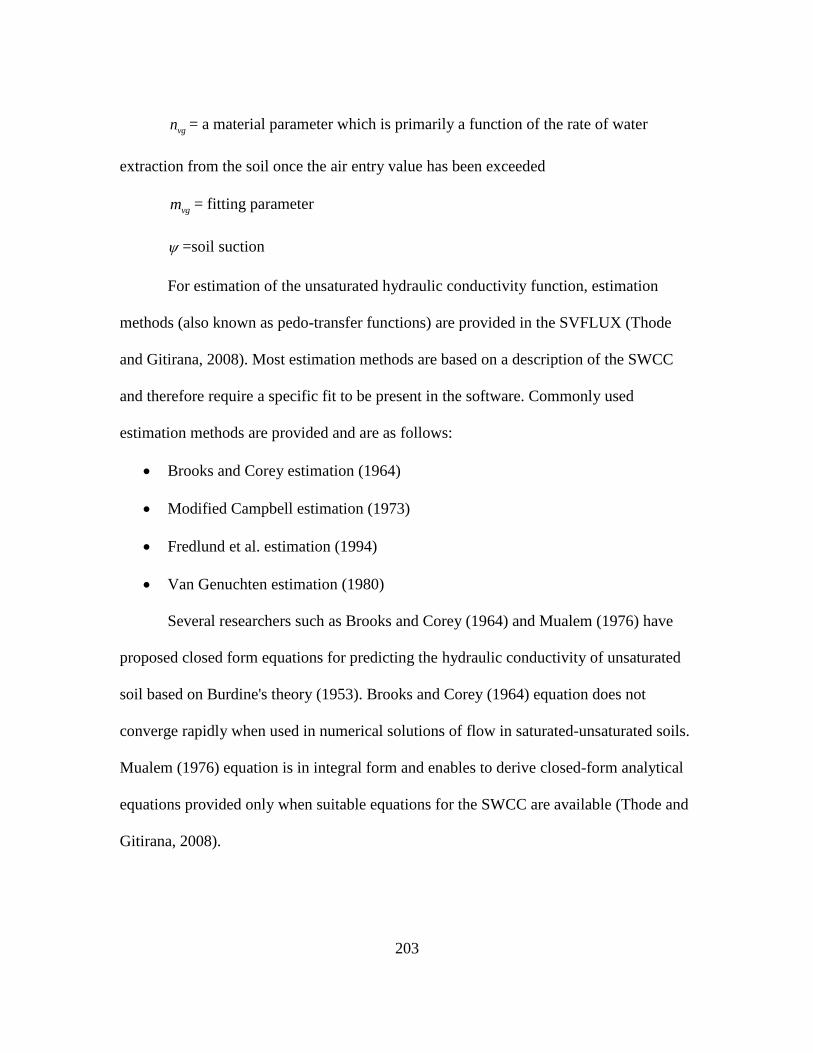
203
vgn = a material parameter which is primarily a function of the rate of water
extraction from the soil once the air entry value has been exceeded
vgm = fitting parameter
=soil suction
For estimation of the unsaturated hydraulic conductivity function, estimation
methods (also known as pedo-transfer functions) are provided in the SVFLUX (Thode
and Gitirana, 2008). Most estimation methods are based on a description of the SWCC
and therefore require a specific fit to be present in the software. Commonly used
estimation methods are provided and are as follows:
Brooks and Corey estimation (1964)
Modified Campbell estimation (1973)
Fredlund et al. estimation (1994)
Van Genuchten estimation (1980)
Several researchers such as Brooks and Corey (1964) and Mualem (1976) have
proposed closed form equations for predicting the hydraulic conductivity of unsaturated
soil based on Burdine's theory (1953). Brooks and Corey (1964) equation does not
converge rapidly when used in numerical solutions of flow in saturated-unsaturated soils.
Mualem (1976) equation is in integral form and enables to derive closed-form analytical
equations provided only when suitable equations for the SWCC are available (Thode and
Gitirana, 2008).
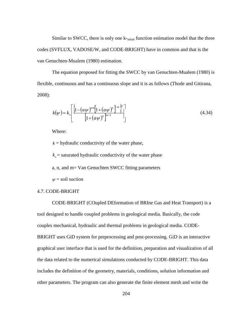
204
Similar to SWCC, there is only one k-unsat function estimation model that the three
codes (SVFLUX, VADOSE/W, and CODE-BRIGHT) have in common and that is the
van Genuchten-Mualem (1980) estimation.
The equation proposed for fitting the SWCC by van Genuchten-Mualem (1980) is
flexible, continuous and has a continuous slope and it is as follows (Thode and Gitirana,
2008):
2/
2
1
11mn
mnnm
s
a
aakk
(4.34)
Where:
k = hydraulic conductivity of the water phase,
sk = saturated hydraulic conductivity of the water phase
a, n, and m= Van Genuchten SWCC fitting parameters
= soil suction
4.7. CODE-BRIGHT
CODE-BRIGHT (COupled DEformation of BRIne Gas and Heat Transport) is a
tool designed to handle coupled problems in geological media. Basically, the code
couples mechanical, hydraulic and thermal problems in geological media. CODE-
BRIGHT uses GiD system for preprocessing and post-processing. GiD is an interactive
graphical user interface that is used for the definition, preparation and visualization of all
the data related to the numerical simulations conducted by CODE-BRIGHT. This data
includes the definition of the geometry, materials, conditions, solution information and
other parameters. The program can also generate the finite element mesh and write the
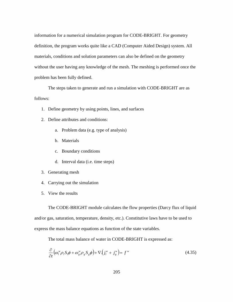
205
information for a numerical simulation program for CODE-BRIGHT. For geometry
definition, the program works quite like a CAD (Computer Aided Design) system. All
materials, conditions and solution parameters can also be defined on the geometry
without the user having any knowledge of the mesh. The meshing is performed once the
problem has been fully defined.
The steps taken to generate and run a simulation with CODE-BRIGHT are as
follows:
1. Define geometry by using points, lines, and surfaces
2. Define attributes and conditions:
a. Problem data (e.g. type of analysis)
b. Materials
c. Boundary conditions
d. Interval data (i.e. time steps)
3. Generating mesh
4. Carrying out the simulation
5. View the results
The CODE-BRIGHT module calculates the flow properties (Darcy flux of liquid
and/or gas, saturation, temperature, density, etc.). Constitutive laws have to be used to
express the mass balance equations as function of the state variables.
The total mass balance of water in CODE-BRIGHT is expressed as:
ww
g
w
lgg
w
gll
w
l fjjSSt
. (4.35)
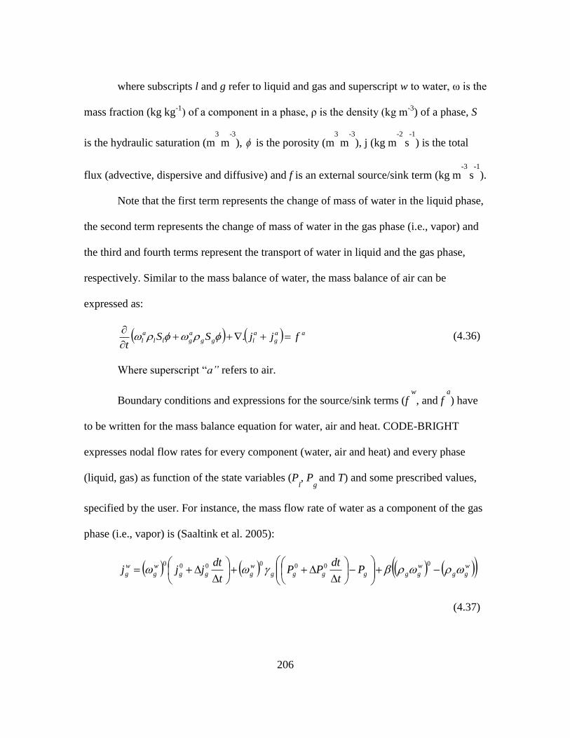
206
where subscripts l and g refer to liquid and gas and superscript w to water, ω is the
mass fraction (kg kg-1
) of a component in a phase, ρ is the density (kg m-3
) of a phase, S
is the hydraulic saturation (m3
m-3
), is the porosity (m3
m-3
), j (kg m-2
s-1
) is the total
flux (advective, dispersive and diffusive) and f is an external source/sink term (kg m-3
s-1
).
Note that the first term represents the change of mass of water in the liquid phase,
the second term represents the change of mass of water in the gas phase (i.e., vapor) and
the third and fourth terms represent the transport of water in liquid and the gas phase,
respectively. Similar to the mass balance of water, the mass balance of air can be
expressed as:
aa
g
a
lgg
a
gll
a
l fjjSSt
. (4.36)
Where superscript “a” refers to air.
Boundary conditions and expressions for the source/sink terms (f w
, and f a
) have
to be written for the mass balance equation for water, air and heat. CODE-BRIGHT
expresses nodal flow rates for every component (water, air and heat) and every phase
(liquid, gas) as function of the state variables (Pl, P
g and T) and some prescribed values,
specified by the user. For instance, the mass flow rate of water as a component of the gas
phase (i.e., vapor) is (Saaltink et al. 2005):
w
gg
w
gggggg
w
ggg
w
g
w
g Pt
dtPP
t
dtjjj
0000000
(4.37)
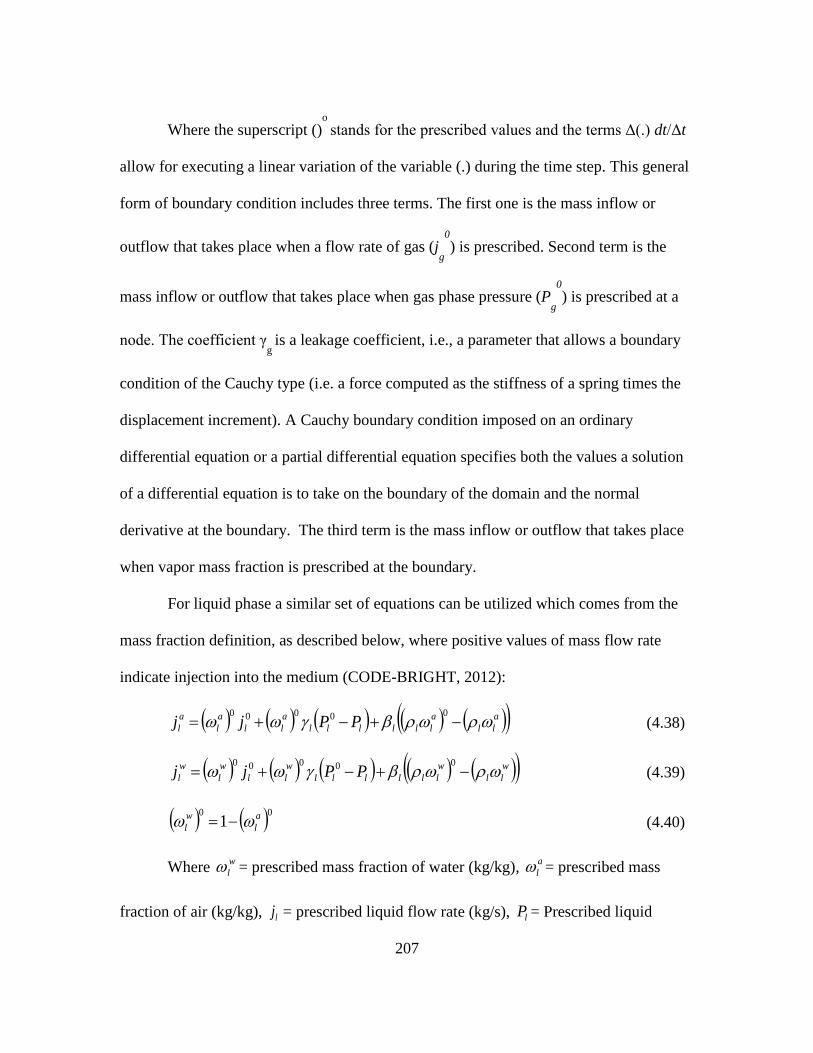
207
Where the superscript ()o
stands for the prescribed values and the terms Δ(.) dt/Δt
allow for executing a linear variation of the variable (.) during the time step. This general
form of boundary condition includes three terms. The first one is the mass inflow or
outflow that takes place when a flow rate of gas (jg
0
) is prescribed. Second term is the
mass inflow or outflow that takes place when gas phase pressure (Pg
0
) is prescribed at a
node. The coefficient γg is a leakage coefficient, i.e., a parameter that allows a boundary
condition of the Cauchy type (i.e. a force computed as the stiffness of a spring times the
displacement increment). A Cauchy boundary condition imposed on an ordinary
differential equation or a partial differential equation specifies both the values a solution
of a differential equation is to take on the boundary of the domain and the normal
derivative at the boundary. The third term is the mass inflow or outflow that takes place
when vapor mass fraction is prescribed at the boundary.
For liquid phase a similar set of equations can be utilized which comes from the
mass fraction definition, as described below, where positive values of mass flow rate
indicate injection into the medium (CODE-BRIGHT, 2012):
a
ll
a
llllll
a
ll
a
l
a
l PPjj 00000
(4.38)
w
ll
w
llllll
w
ll
w
l
w
l PPjj 00000
(4.39)
001 a
l
w
l (4.40)
Where w
l = prescribed mass fraction of water (kg/kg), a
l = prescribed mass
fraction of air (kg/kg), lj = prescribed liquid flow rate (kg/s), lP = Prescribed liquid
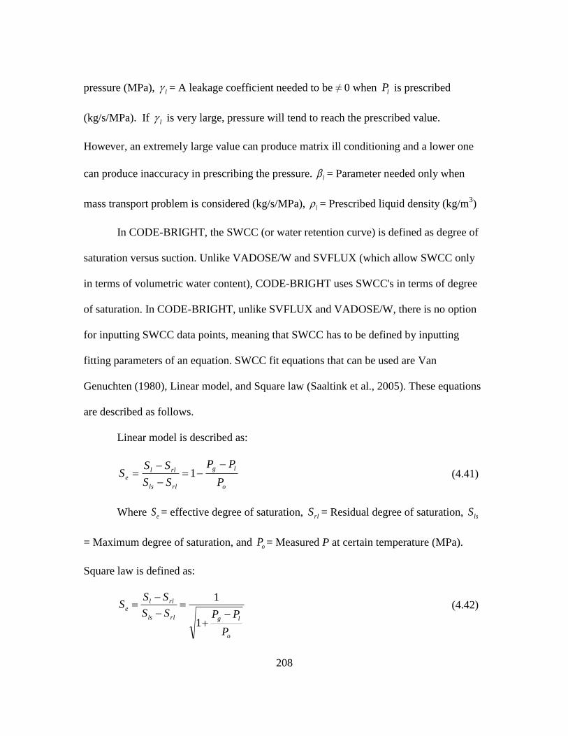
208
pressure (MPa), l = A leakage coefficient needed to be ≠ 0 when lP is prescribed
(kg/s/MPa). If l is very large, pressure will tend to reach the prescribed value.
However, an extremely large value can produce matrix ill conditioning and a lower one
can produce inaccuracy in prescribing the pressure. l = Parameter needed only when
mass transport problem is considered (kg/s/MPa), l = Prescribed liquid density (kg/m3)
In CODE-BRIGHT, the SWCC (or water retention curve) is defined as degree of
saturation versus suction. Unlike VADOSE/W and SVFLUX (which allow SWCC only
in terms of volumetric water content), CODE-BRIGHT uses SWCC's in terms of degree
of saturation. In CODE-BRIGHT, unlike SVFLUX and VADOSE/W, there is no option
for inputting SWCC data points, meaning that SWCC has to be defined by inputting
fitting parameters of an equation. SWCC fit equations that can be used are Van
Genuchten (1980), Linear model, and Square law (Saaltink et al., 2005). These equations
are described as follows.
Linear model is described as:
o
lg
rlls
rll
eP
PP
SS
SSS
1 (4.41)
Where eS = effective degree of saturation, rlS = Residual degree of saturation, lsS
= Maximum degree of saturation, and oP = Measured P at certain temperature (MPa).
Square law is defined as:
o
lgrlls
rlle
P
PPSS
SSS
1
1 (4.42)
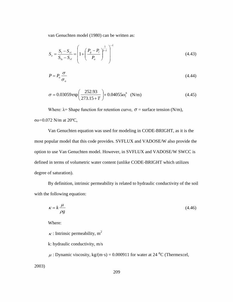
209
van Genuchten model (1980) can be written as:
1
1
1o
lg
rlls
rlle
P
PP
SS
SSS (4.43)
o
oPP
(4.44)
h
lT
04055.015.273
93.252exp03059.0
(N/m) (4.45)
Where: λ= Shape function for retention curve, = surface tension (N/m),
σo=0.072 N/m at 20ºC,
Van Genuchten equation was used for modeling in CODE-BRIGHT, as it is the
most popular model that this code provides. SVFLUX and VADOSE/W also provide the
option to use Van Genuchten model. However, in SVFLUX and VADOSE/W SWCC is
defined in terms of volumetric water content (unlike CODE-BRIGHT which utilizes
degree of saturation).
By definition, intrinsic permeability is related to hydraulic conductivity of the soil
with the following equation:
gk
(4.46)
Where:
: Intrinsic permeability, m2
k: hydraulic conductivity, m/s
: Dynamic viscosity, kg/(m·s) = 0.000911 for water at 24 ⁰C (Thermexcel,
2003)
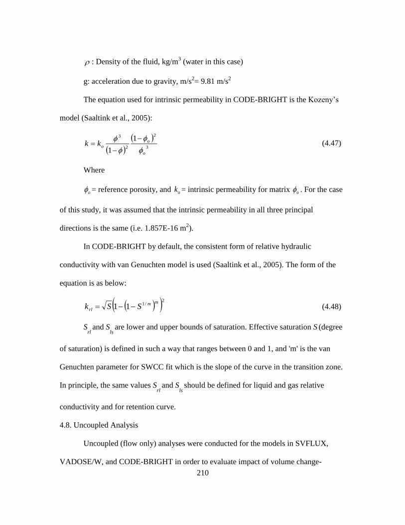
210
: Density of the fluid, kg/m3 (water in this case)
g: acceleration due to gravity, m/s2= 9.81 m/s
2
The equation used for intrinsic permeability in CODE-BRIGHT is the Kozeny’s
model (Saaltink et al., 2005):
3
2
2
3 1
1 o
o
okk
(4.47)
Where
o = reference porosity, and ok = intrinsic permeability for matrix o . For the case
of this study, it was assumed that the intrinsic permeability in all three principal
directions is the same (i.e. 1.857E-16 m2).
In CODE-BRIGHT by default, the consistent form of relative hydraulic
conductivity with van Genuchten model is used (Saaltink et al., 2005). The form of the
equation is as below:
2/111mm
rl SSk (4.48)
Srl
and Sls
are lower and upper bounds of saturation. Effective saturation S (degree
of saturation) is defined in such a way that ranges between 0 and 1, and 'm' is the van
Genuchten parameter for SWCC fit which is the slope of the curve in the transition zone.
In principle, the same values Srl
and Sls
should be defined for liquid and gas relative
conductivity and for retention curve.
4.8. Uncoupled Analysis
Uncoupled (flow only) analyses were conducted for the models in SVFLUX,
VADOSE/W, and CODE-BRIGHT in order to evaluate impact of volume change-
211
corrected SWCC on computed hydraulic properties of soils and on soil suction profiles
(e.g. progression of wetted front, degree of wetting), and hence soil volume change due to
wetting for expansive clays. The rate of change of suction, including for infiltration cases,
the progression of the wetted front was studied and the amount of suction-induced
volume change was determined based on the generated suction profile of the soil column.
For this purpose, suction compression curves (void ratio versus suction) of specimens
obtained from SWCC laboratory experiments were utilized.
For the steady-state uncoupled analyses, boundary conditions only needed to be
defined for the model. These boundary conditions included the flow/head conditions
explained in earlier sections of this chapter. The boundary conditions were set in the way
that the left and right (vertical) sides have no flow (No-flux boundary condition), while
the bottom has a constant pressure head (e.g. -10m) and at the top the boundary condition
is either fixed flux (with values varying from evaporation to positive flux of magnitude
much less than saturated hydraulic conductivity (k-sat) of the soil to values greater than k-
sat) or fixed head of 1m.
For transient uncoupled analysis, however, in addition to the mentioned boundary
conditions, initial conditions of the model must also be defined. For the majority of cases,
as the initial suction profile of the model, it was assumed that the soil is unsaturated with
groundwater located 10 meters below the bottom of the soil column. This initial suction
profile is shown in Figure 4.13. It can be seen that the initial suction at the bottom of the
soil column is -100kPa and the initial suction at the top of the soil column is -600kPa.
The suction variation between these two points changes linearly. After the initial
212
flow/head has been set, the fixed head/fixed flux is added at the top of the soil column.
By doing this, the initially unsaturated soil starts to become wet from the top. By setting
appropriate time steps, progression of wetted front can be estimated through transient
uncoupled analysis.
The computer codes used for unsaturated flow modeling generate the suction
profile for the various models. Based on the generated suction profile and by using the
suction compression curves which is available for soils Anthem, Colorado, and San
Antonio through the SWCC tests, initial and final void ratio profiles can be estimated. By
having initial and final values of void ratio, amount of suction-change induced
deformation can be calculated.
It should be mentioned that for the case of Anthem, Colorado, and San Antonio
soils, the ksat value was assumed to be constant. In other words, ksat was not updated for
changes in void ratio. Given the amount of volume change experienced by the compacted
specimens of expansive clays studied here, this would not be expected to result in big
differences in ksat due to change in void ratio. However, this is not true for slurry
specimens or any other soils having extremely high volume change. Issues related to ksat
changes and volume changes for soil suction change below the AEV are the next chapter
which focuses on extremely high volume change slurry materials.
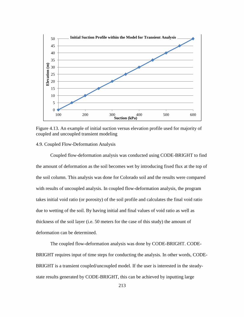
213
Figure 4.13. An example of initial suction versus elevation profile used for majority of
coupled and uncoupled transient modeling
4.9. Coupled Flow-Deformation Analysis
Coupled flow-deformation analysis was conducted using CODE-BRIGHT to find
the amount of deformation as the soil becomes wet by introducing fixed flux at the top of
the soil column. This analysis was done for Colorado soil and the results were compared
with results of uncoupled analysis. In coupled flow-deformation analysis, the program
takes initial void ratio (or porosity) of the soil profile and calculates the final void ratio
due to wetting of the soil. By having initial and final values of void ratio as well as
thickness of the soil layer (i.e. 50 meters for the case of this study) the amount of
deformation can be determined.
The coupled flow-deformation analysis was done by CODE-BRIGHT. CODE-
BRIGHT requires input of time steps for conducting the analysis. In other words, CODE-
BRIGHT is a transient coupled/uncoupled model. If the user is interested in the steady-
state results generated by CODE-BRIGHT, this can be achieved by inputting large
0
5
10
15
20
25
30
35
40
45
50
100 200 300 400 500 600
Ele
va
tio
n (
m)
Suction (kPa)
Initial Suction Profile within the Model for Transient Analysis
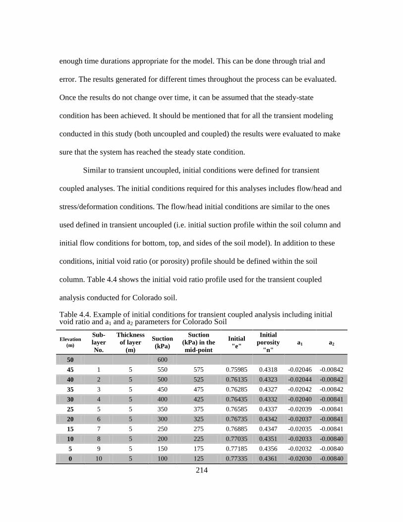
214
enough time durations appropriate for the model. This can be done through trial and
error. The results generated for different times throughout the process can be evaluated.
Once the results do not change over time, it can be assumed that the steady-state
condition has been achieved. It should be mentioned that for all the transient modeling
conducted in this study (both uncoupled and coupled) the results were evaluated to make
sure that the system has reached the steady state condition.
Similar to transient uncoupled, initial conditions were defined for transient
coupled analyses. The initial conditions required for this analyses includes flow/head and
stress/deformation conditions. The flow/head initial conditions are similar to the ones
used defined in transient uncoupled (i.e. initial suction profile within the soil column and
initial flow conditions for bottom, top, and sides of the soil model). In addition to these
conditions, initial void ratio (or porosity) profile should be defined within the soil
column. Table 4.4 shows the initial void ratio profile used for the transient coupled
analysis conducted for Colorado soil.
Table 4.4. Example of initial conditions for transient coupled analysis including initial void ratio and a1 and a2 parameters for Colorado Soil
Elevation
(m)
Sub-
layer
No.
Thickness
of layer
(m)
Suction
(kPa)
Suction
(kPa) in the
mid-point
Initial
"e"
Initial
porosity
"n"
a1 a2
50
600
45 1 5 550 575 0.75985 0.4318 -0.02046 -0.00842
40 2 5 500 525 0.76135 0.4323 -0.02044 -0.00842
35 3 5 450 475 0.76285 0.4327 -0.02042 -0.00842
30 4 5 400 425 0.76435 0.4332 -0.02040 -0.00841
25 5 5 350 375 0.76585 0.4337 -0.02039 -0.00841
20 6 5 300 325 0.76735 0.4342 -0.02037 -0.00841
15 7 5 250 275 0.76885 0.4347 -0.02035 -0.00841
10 8 5 200 225 0.77035 0.4351 -0.02033 -0.00840
5 9 5 150 175 0.77185 0.4356 -0.02032 -0.00840
0 10 5 100 125 0.77335 0.4361 -0.02030 -0.00840
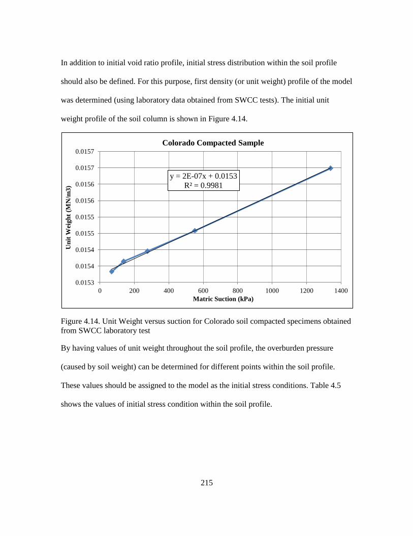
215
In addition to initial void ratio profile, initial stress distribution within the soil profile
should also be defined. For this purpose, first density (or unit weight) profile of the model
was determined (using laboratory data obtained from SWCC tests). The initial unit
weight profile of the soil column is shown in Figure 4.14.
Figure 4.14. Unit Weight versus suction for Colorado soil compacted specimens obtained
from SWCC laboratory test
By having values of unit weight throughout the soil profile, the overburden pressure
(caused by soil weight) can be determined for different points within the soil profile.
These values should be assigned to the model as the initial stress conditions. Table 4.5
shows the values of initial stress condition within the soil profile.
y = 2E-07x + 0.0153
R² = 0.9981
0.0153
0.0154
0.0154
0.0155
0.0155
0.0156
0.0156
0.0157
0.0157
0 200 400 600 800 1000 1200 1400
Un
it W
eig
ht
(MN
/m3
)
Matric Suction (kPa)
Colorado Compacted Sample
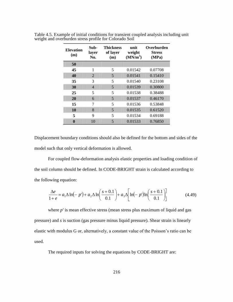
216
Table 4.5. Example of initial conditions for transient coupled analysis including unit weight and overburden stress profile for Colorado Soil
Elevation
(m)
Sub-
layer
No.
Thickness
of layer
(m)
unit
weight
(MN/m3)
Overburden
Stress
(MPa)
50
45 1 5 0.01542 0.07708
40 2 5 0.01541 0.15410
35 3 5 0.01540 0.23108
30 4 5 0.01539 0.30800
25 5 5 0.01538 0.38488
20 6 5 0.01537 0.46170
15 7 5 0.01536 0.53848
10 8 5 0.01535 0.61520
5 9 5 0.01534 0.69188
0 10 5 0.01533 0.76850
Displacement boundary conditions should also be defined for the bottom and sides of the
model such that only vertical deformation is allowed.
For coupled flow-deformation analysis elastic properties and loading condition of
the soil column should be defined. In CODE-BRIGHT strain is calculated according to
the following equation:
1.0
1.0ln'ln
1.0
1.0ln'ln
1321
spa
sapa
e
e (4.49)
where p' is mean effective stress (mean stress plus maximum of liquid and gas
pressure) and s is suction (gas pressure minus liquid pressure). Shear strain is linearly
elastic with modulus G or, alternatively, a constant value of the Poisson’s ratio can be
used.
The required inputs for solving the equations by CODE-BRIGHT are:
217
1. e
a
11
where is the slope of the unload/reload curve in the (e - lnp')
diagram
2. e
a s
12
where s is the slope of the unload/reload curve in the (e -
1.0
1.0ln
s)
diagram
3. 3a can be set as zero, which assumes that suction does not have a direct impact on
the mean stress
4. = Poisson’s ratio.
Determining 1a :
For finding value of1a , should be determined. By definition, is the slope of
unloading-reloading line (url) in void ration versus ln p' space (e - lnp'), where
3/' '
3
'
2
'
1 p . This is shown in Figure 4.15 (Muir Wood, 1991). In this figure
stands for void ratio (usually called 'e' in the literature). Another method to illustrate load-
compression curve is to the curve showing void ratio versus log'
v . This is usually
obtained from one-dimensional compression test in oedometer device (shown in Figure
4.16). Slopes of loading and reloading curves in Figure 4.16 are often measured and are
called compression index ( cC ) and swelling index ( sC ). Swelling index ( sC ) is also
referred to as recompression index (rC ) (Holtz et al. 2010).
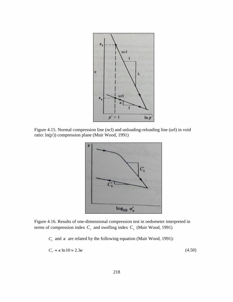
218
Figure 4.15. Normal compression line (ncl) and unloading-reloading line (url) in void
ratio: ln(p')) compression plane (Muir Wood, 1991)
Figure 4.16. Results of one-dimensional compression test in oedometer interpreted in
terms of compression index cC and swelling index sC (Muir Wood, 1991)
rC and are related by the following equation (Muir Wood, 1991):
3.210ln rC (4.50)
219
There are equations developed by researchers in the literature to estimate rC for
different soil types. For the case of Colorado soil, equation below which was developed
by Nagaraj and Murthy (1985) was used to estimate value of rC :
sLLr GwC 000463.0 (4.51)
Where LLw is the liquid limit of the soil and sG is the specific gravity. For
Colorado soil rC is determined to be around 0.083 as follows:
0.0842.77865000463.0000463.0 sLLr GwC
By having value of rC , can be calculated by equation:
036.03.2
084.0
3.2 rC
(4.52)
As mentioned previously, void ratio of Colorado soil can be calculated by
knowing the values of Gs (specific gravity) and volumetric water content at saturation
(0.3 for Colorado soil).
wGeS s (4.53)
Where S is the degree of saturation, e is the void ratio, and w is the water content.
At saturation, e can be calculated as: 83.01
3.0778.2
S
wGe s
By having values of and void ratio, 1a can be calculated as:
0197.0
83.01
036.0
11
ea
220
Determining2a :
As previously mentioned, e
a s
12
where s is the slope of the unload/reload
curve in the (e -
1.0
1.0ln
s) diagram. In other words s is the suction compression index
when suction is plotted on a semi-natural log scale. The Suction Compression Index, Cs,
is the change in soil volume for a 1- log cycle change in suction. The magnitude of the
suction compression index indicates if the soil is expansive or not. Small slope
characterizes a swelling soil while a large slope indicates a non-expansive soil (Dye
2008).
Determination of the suction compression index is necessary for predicting the
suction-change induced deformation of expansive soils (Perko et al. 2000). The suction
compression index, s or as sometimes referred to as Cs when determined on void ratio
versus log suction plot, can be measured using 1-D laboratory tests .
s is the slope of suction compression curve in the semi-logarithmic space (e -
1.0
1.0ln
s).
For the soil in this study (Anthem, Colorado, and San Antonio), suction
compression curve was measured. Table 4.6 shows part of the void ratio versus matric
suction measured during SWCC test of Colorado soil.
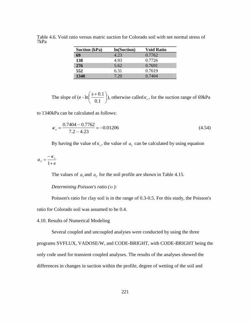
221
Table 4.6. Void ratio versus matric suction for Colorado soil with net normal stress of 7kPa
Suction (kPa) ln(Suction) Void Ratio
69 4.23 0.7762
138 4.93 0.7726
276 5.62 0.7691
552 6.31 0.7619
1340 7.20 0.7404
The slope of (e -
1.0
1.0ln
s), otherwise called s , for the suction range of 69kPa
to 1340kPa can be calculated as follows:
0.0120623.42.7
7762.07404.0
s (4.54)
By having the value of s , the value of 2a can be calculated by using equation
ea s
12
The values of 1a and
2a for the soil profile are shown in Table 4.15.
Determining Poisson's ratio ( ):
Poisson's ratio for clay soil is in the range of 0.3-0.5. For this study, the Poisson's
ratio for Colorado soil was assumed to be 0.4.
4.10. Results of Numerical Modeling
Several coupled and uncoupled analyses were conducted by using the three
programs SVFLUX, VADOSE/W, and CODE-BRIGHT, with CODE-BRIGHT being the
only code used for transient coupled analyses. The results of the analyses showed the
differences in changes in suction within the profile, degree of wetting of the soil and
222
amount of deformation for both volume-corrected and volume-uncorrected SWCC's. The
details of the results of the analyses are presented in the following section.
4.10.1. Results of Uncoupled Analyses
Transient and steady-state analyses were conducted by SVFLUX, VADOSE/W,
and CODE-BRIGHT in which a soil column becomes wet (positive flux) or dry (negative
flux) from top with either fixed flux or fixed head. The results of the flow-only
(uncoupled) analyses are presented in this section.
4.10.1.1. Anthem Soil
Table 4.7 provides a list of numerical modeling conducted on the models based on
the properties of Anthem soil. Simulations were run using Anthem soil properties. Figure
4.17 through 4.20 show results of transient uncoupled analyses using CODE-BRIGHT
for Anthem soil. The top boundary condition for this set of runs was fixed flux of 1.0E-3
m/day. Results of the analyses showed that at stead-state condition (i.e. at the time that
the model has become saturated due to the positive flux at the top) in the case modeled
with uncorrected SWCC the suction throughout the soil column is smaller compared to
the one with corrected SWCC (suction of 10kPa for uncorrected SWCC versus 26kPa for
corrected SWCC for the majority of the soil profile). However, for a time before the
model reaches the steady-state (e.g. 4000 days shown in Figure 4.19) the uncorrected
case shows higher suction values at some of the points within the soil profile. This is due
to the fact that the progression of wetted front has a higher rate for corrected SWCC
compared to uncorrected SWCC. As shown in Figure 4.19 at the elevations between 7m
and 15m (from the datum which is located at the bottom of the soil layer), the values of
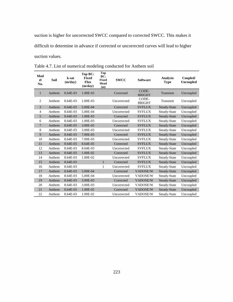
223
suction is higher for uncorrected SWCC compared to corrected SWCC. This makes it
difficult to determine in advance if corrected or uncorrected curves will lead to higher
suction values.
Table 4.7. List of numerical modeling conducted for Anthem soil
Mod
el
No.
Soil k-sat
(m/day)
Top BC:
Fixed
Flux
(m/day)
Top
BC:
Fixed
Head
(m)
SWCC Software Analysis
Type
Coupled/
Uncoupled
1 Anthem 8.64E-03 1.00E-03
Corrected CODE-
BRIGHT Transient Uncoupled
2 Anthem 8.64E-03 1.00E-03
Uncorrected CODE-
BRIGHT Transient Uncoupled
3 Anthem 8.64E-03 5.00E-04
Corrected SVFLUX Steady-State Uncoupled
4 Anthem 8.64E-03 5.00E-04
Uncorrected SVFLUX Steady-State Uncoupled
5 Anthem 8.64E-03 1.00E-03
Corrected SVFLUX Steady-State Uncoupled
6 Anthem 8.64E-03 1.00E-03
Uncorrected SVFLUX Steady-State Uncoupled
7 Anthem 8.64E-03 3.00E-03
Corrected SVFLUX Steady-State Uncoupled
8 Anthem 8.64E-03 3.00E-03
Uncorrected SVFLUX Steady-State Uncoupled
9 Anthem 8.64E-03 7.00E-03
Corrected SVFLUX Steady-State Uncoupled
10 Anthem 8.64E-03 7.00E-03
Uncorrected SVFLUX Steady-State Uncoupled
11 Anthem 8.64E-03 8.64E-03
Corrected SVFLUX Steady-State Uncoupled
12 Anthem 8.64E-03 8.64E-03
Uncorrected SVFLUX Steady-State Uncoupled
13 Anthem 8.64E-03 1.00E-02
Corrected SVFLUX Steady-State Uncoupled
14 Anthem 8.64E-03 1.00E-02
Uncorrected SVFLUX Steady-State Uncoupled
15 Anthem 8.64E-03
1 Corrected SVFLUX Steady-State Uncoupled
16 Anthem 8.64E-03
1 Uncorrected SVFLUX Steady-State Uncoupled
17 Anthem 8.64E-03 5.00E-04
Corrected VADOSE/W Steady-State Uncoupled
18 Anthem 8.64E-03 5.00E-04
Uncorrected VADOSE/W Steady-State Uncoupled
19 Anthem 8.64E-03 3.00E-03
Corrected VADOSE/W Steady-State Uncoupled
20 Anthem 8.64E-03 3.00E-03
Uncorrected VADOSE/W Steady-State Uncoupled
21 Anthem 8.64E-03 1.00E-02
Corrected VADOSE/W Steady-State Uncoupled
22 Anthem 8.64E-03 1.00E-02
Uncorrected VADOSE/W Steady-State Uncoupled
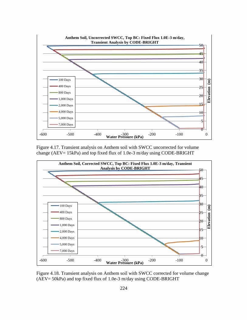
224
Figure 4.17. Transient analysis on Anthem soil with SWCC uncorrected for volume
change (AEV= 15kPa) and top fixed flux of 1.0e-3 m/day using CODE-BRIGHT
Figure 4.18. Transient analysis on Anthem soil with SWCC corrected for volume change
(AEV= 50kPa) and top fixed flux of 1.0e-3 m/day using CODE-BRIGHT
0
5
10
15
20
25
30
35
40
45
50
-600 -500 -400 -300 -200 -100 0
Ele
va
tio
n (m
)
Water Pressure (kPa)
Anthem Soil, Uncorrected SWCC, Top BC: Fixed Flux 1.0E-3 m/day,
Transient Analysis by CODE-BRIGHT
100 Days
400 Days
800 Days
1,000 Days
2,000 Days
4,000 Days
5,000 Days
7,000 Days
0
5
10
15
20
25
30
35
40
45
50
-600 -500 -400 -300 -200 -100 0
Ele
va
tio
n (m
)
Water Pressure (kPa)
Anthem Soil, Corrected SWCC, Top BC: Fixed Flux 1.0E-3 m/day, Transient
Analysis by CODE-BRIGHT
100 Days
400 Days
800 Days
1,000 Days
2,000 Days
4,000 Days
5,000 Days
7,000 Days
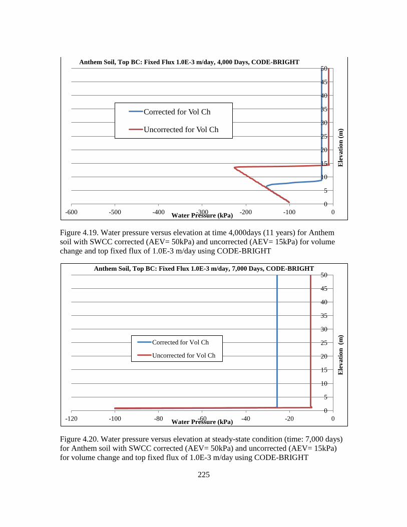
225
Figure 4.19. Water pressure versus elevation at time 4,000days (11 years) for Anthem
soil with SWCC corrected (AEV= 50kPa) and uncorrected (AEV= 15kPa) for volume
change and top fixed flux of 1.0E-3 m/day using CODE-BRIGHT
Figure 4.20. Water pressure versus elevation at steady-state condition (time: 7,000 days)
for Anthem soil with SWCC corrected (AEV= 50kPa) and uncorrected (AEV= 15kPa)
for volume change and top fixed flux of 1.0E-3 m/day using CODE-BRIGHT
0
5
10
15
20
25
30
35
40
45
50
-600 -500 -400 -300 -200 -100 0
Ele
va
tio
n (
m)
Water Pressure (kPa)
Anthem Soil, Top BC: Fixed Flux 1.0E-3 m/day, 4,000 Days, CODE-BRIGHT
Corrected for Vol Ch
Uncorrected for Vol Ch
0
5
10
15
20
25
30
35
40
45
50
-120 -100 -80 -60 -40 -20 0
Ele
va
tio
n (m
)
Water Pressure (kPa)
Anthem Soil, Top BC: Fixed Flux 1.0E-3 m/day, 7,000 Days, CODE-BRIGHT
Corrected for Vol Ch
Uncorrected for Vol Ch

226
4.10.1.2. Colorado Soil
Table 4.8 provides a list of numerical modeling conducted based on Colorado soil
properties. Figures 4.21 through 4.31 show results of modeling using Colorado soil.
Similar result trends to Anthem soil were found for Colorado soil. At the times long-
enough for the model to reach the steady-state (i.e. saturated in this case), the model
based on uncorrected SWCC shows smaller final suction throughout the soil column
compared to the model based on corrected SWCC (suction of 15kPa for uncorrected
SWCC versus 28kPa for corrected SWCC for the majority of the soil profile). In addition,
the rate of progression of wetted front is larger for the case of SWCC corrected for
volume change due to larger unsaturated hydraulic conductivity values. This leads to
higher suctions at some points within the soil profile (for the times prior to steady-state)
for uncorrected SWCC. This is shown in Figure 4.23 which illustrates the suction profile
of both corrected and uncorrected SWCC models at time 7,000 days. It can be seen that at
this time, at the elevations between 10m and 25m (from the bottom of the soil column),
the values of suction is higher for uncorrected SWCC. Similar to observed results from
the runs on Anthem soil, this makes it difficult to determine in advance if corrected or
uncorrected curves will lead to higher suction values.
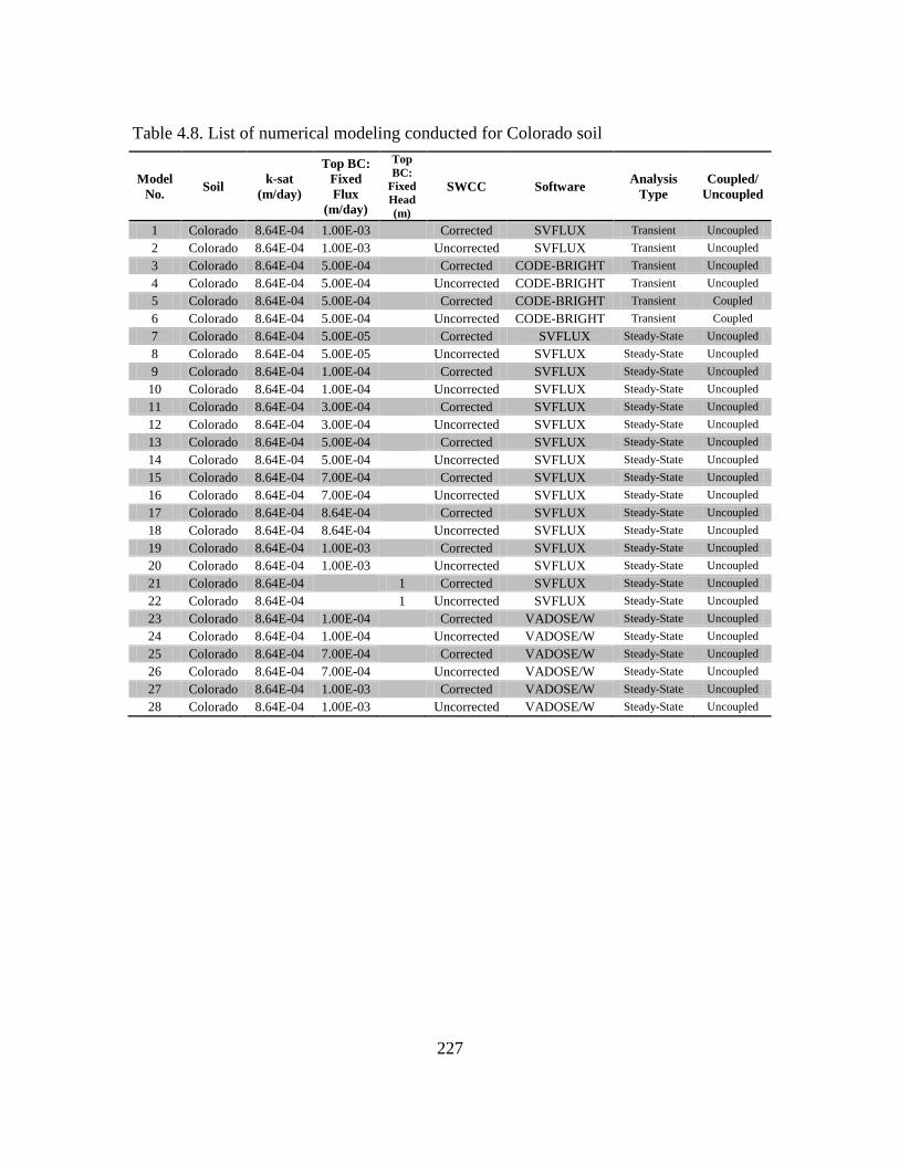
227
Table 4.8. List of numerical modeling conducted for Colorado soil
Model
No. Soil
k-sat
(m/day)
Top BC:
Fixed
Flux
(m/day)
Top
BC:
Fixed
Head
(m)
SWCC Software Analysis
Type
Coupled/
Uncoupled
1 Colorado 8.64E-04 1.00E-03
Corrected SVFLUX Transient Uncoupled
2 Colorado 8.64E-04 1.00E-03
Uncorrected SVFLUX Transient Uncoupled
3 Colorado 8.64E-04 5.00E-04
Corrected CODE-BRIGHT Transient Uncoupled
4 Colorado 8.64E-04 5.00E-04
Uncorrected CODE-BRIGHT Transient Uncoupled
5 Colorado 8.64E-04 5.00E-04
Corrected CODE-BRIGHT Transient Coupled
6 Colorado 8.64E-04 5.00E-04
Uncorrected CODE-BRIGHT Transient Coupled
7 Colorado 8.64E-04 5.00E-05
Corrected SVFLUX Steady-State Uncoupled
8 Colorado 8.64E-04 5.00E-05
Uncorrected SVFLUX Steady-State Uncoupled
9 Colorado 8.64E-04 1.00E-04
Corrected SVFLUX Steady-State Uncoupled
10 Colorado 8.64E-04 1.00E-04
Uncorrected SVFLUX Steady-State Uncoupled
11 Colorado 8.64E-04 3.00E-04
Corrected SVFLUX Steady-State Uncoupled
12 Colorado 8.64E-04 3.00E-04
Uncorrected SVFLUX Steady-State Uncoupled
13 Colorado 8.64E-04 5.00E-04
Corrected SVFLUX Steady-State Uncoupled
14 Colorado 8.64E-04 5.00E-04
Uncorrected SVFLUX Steady-State Uncoupled
15 Colorado 8.64E-04 7.00E-04
Corrected SVFLUX Steady-State Uncoupled
16 Colorado 8.64E-04 7.00E-04
Uncorrected SVFLUX Steady-State Uncoupled
17 Colorado 8.64E-04 8.64E-04
Corrected SVFLUX Steady-State Uncoupled
18 Colorado 8.64E-04 8.64E-04
Uncorrected SVFLUX Steady-State Uncoupled
19 Colorado 8.64E-04 1.00E-03
Corrected SVFLUX Steady-State Uncoupled
20 Colorado 8.64E-04 1.00E-03
Uncorrected SVFLUX Steady-State Uncoupled
21 Colorado 8.64E-04
1 Corrected SVFLUX Steady-State Uncoupled
22 Colorado 8.64E-04
1 Uncorrected SVFLUX Steady-State Uncoupled
23 Colorado 8.64E-04 1.00E-04
Corrected VADOSE/W Steady-State Uncoupled
24 Colorado 8.64E-04 1.00E-04
Uncorrected VADOSE/W Steady-State Uncoupled
25 Colorado 8.64E-04 7.00E-04
Corrected VADOSE/W Steady-State Uncoupled
26 Colorado 8.64E-04 7.00E-04
Uncorrected VADOSE/W Steady-State Uncoupled
27 Colorado 8.64E-04 1.00E-03
Corrected VADOSE/W Steady-State Uncoupled
28 Colorado 8.64E-04 1.00E-03
Uncorrected VADOSE/W Steady-State Uncoupled
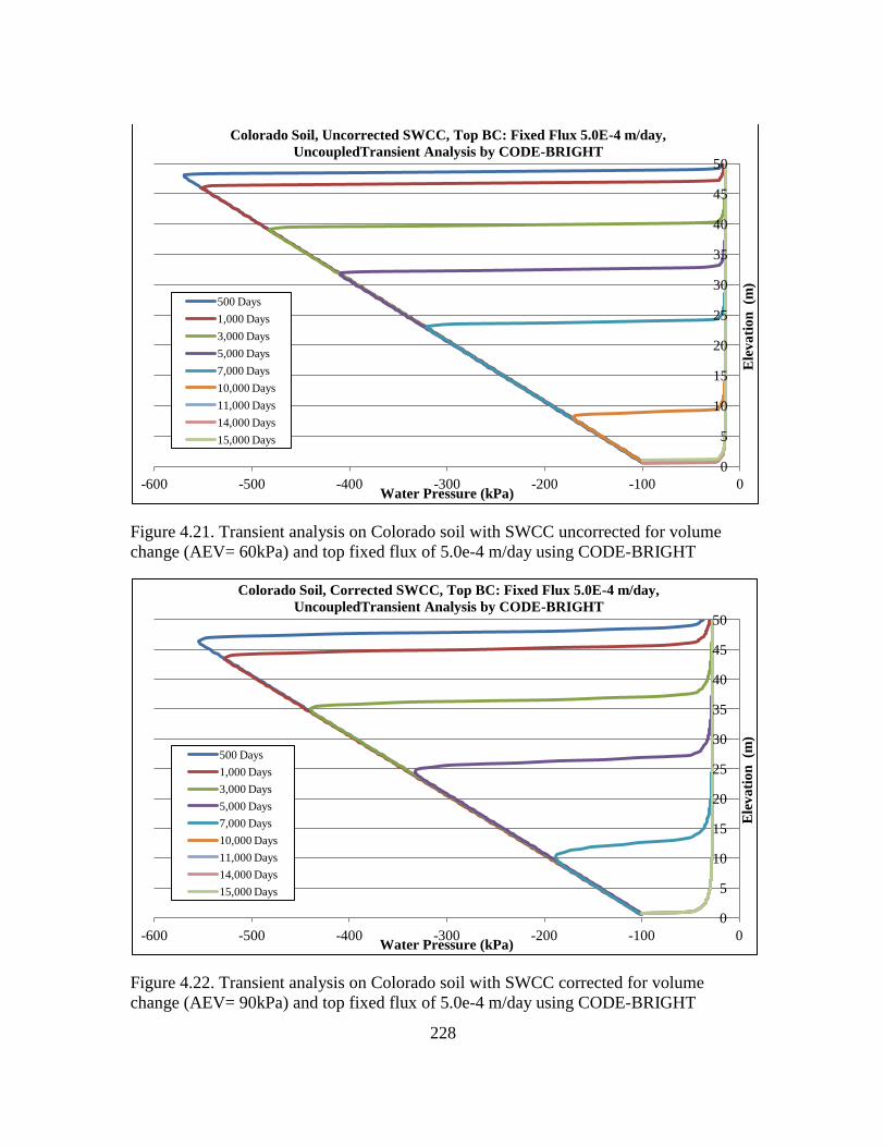
228
Figure 4.21. Transient analysis on Colorado soil with SWCC uncorrected for volume
change (AEV= 60kPa) and top fixed flux of 5.0e-4 m/day using CODE-BRIGHT
Figure 4.22. Transient analysis on Colorado soil with SWCC corrected for volume
change (AEV= 90kPa) and top fixed flux of 5.0e-4 m/day using CODE-BRIGHT
0
5
10
15
20
25
30
35
40
45
50
-600 -500 -400 -300 -200 -100 0
Ele
va
tio
n (m
)
Water Pressure (kPa)
Colorado Soil, Uncorrected SWCC, Top BC: Fixed Flux 5.0E-4 m/day,
UncoupledTransient Analysis by CODE-BRIGHT
500 Days
1,000 Days
3,000 Days
5,000 Days
7,000 Days
10,000 Days
11,000 Days
14,000 Days
15,000 Days
0
5
10
15
20
25
30
35
40
45
50
-600 -500 -400 -300 -200 -100 0
Ele
va
tio
n (m
)
Water Pressure (kPa)
Colorado Soil, Corrected SWCC, Top BC: Fixed Flux 5.0E-4 m/day,
UncoupledTransient Analysis by CODE-BRIGHT
500 Days
1,000 Days
3,000 Days
5,000 Days
7,000 Days
10,000 Days
11,000 Days
14,000 Days
15,000 Days
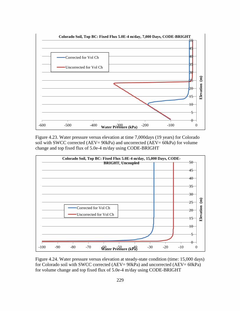
229
Figure 4.23. Water pressure versus elevation at time 7,000days (19 years) for Colorado
soil with SWCC corrected (AEV= 90kPa) and uncorrected (AEV= 60kPa) for volume
change and top fixed flux of 5.0e-4 m/day using CODE-BRIGHT
Figure 4.24. Water pressure versus elevation at steady-state condition (time: 15,000 days)
for Colorado soil with SWCC corrected (AEV= 90kPa) and uncorrected (AEV= 60kPa)
for volume change and top fixed flux of 5.0e-4 m/day using CODE-BRIGHT
0
5
10
15
20
25
30
35
40
45
50
-600 -500 -400 -300 -200 -100 0
Ele
va
tio
n (m
)
Water Pressure (kPa)
Colorado Soil, Top BC: Fixed Flux 5.0E-4 m/day, 7,000 Days, CODE-BRIGHT
Corrected for Vol Ch
Uncorrected for Vol Ch
0
5
10
15
20
25
30
35
40
45
50
-100 -90 -80 -70 -60 -50 -40 -30 -20 -10 0
Ele
va
tio
n (m
)
Water Pressure (kPa)
Colorado Soil, Top BC: Fixed Flux 5.0E-4 m/day, 15,000 Days, CODE-
BRIGHT, Uncoupled
Corrected for Vol Ch
Uncorrected for Vol Ch
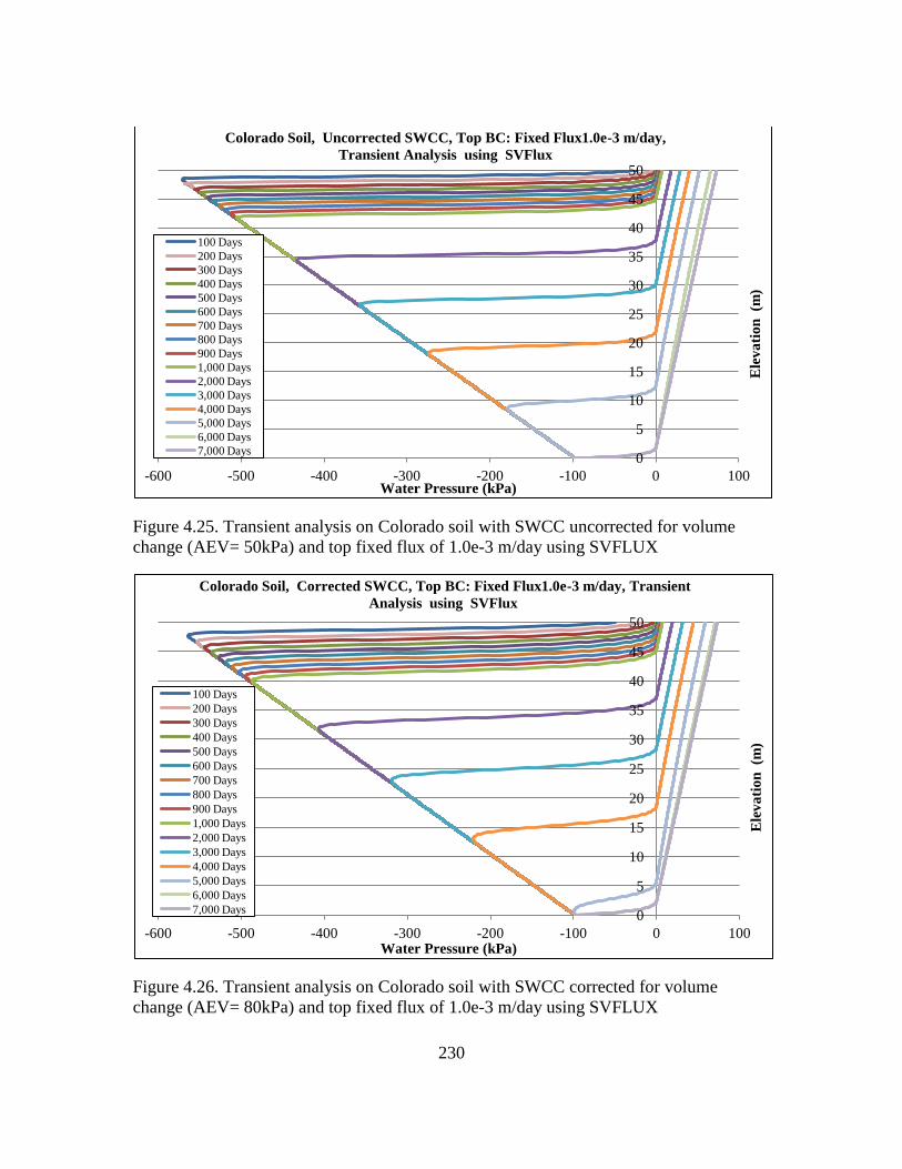
230
Figure 4.25. Transient analysis on Colorado soil with SWCC uncorrected for volume
change (AEV= 50kPa) and top fixed flux of 1.0e-3 m/day using SVFLUX
Figure 4.26. Transient analysis on Colorado soil with SWCC corrected for volume
change (AEV= 80kPa) and top fixed flux of 1.0e-3 m/day using SVFLUX
0
5
10
15
20
25
30
35
40
45
50
-600 -500 -400 -300 -200 -100 0 100
Ele
va
tio
n (m
)
Water Pressure (kPa)
Colorado Soil, Uncorrected SWCC, Top BC: Fixed Flux1.0e-3 m/day,
Transient Analysis using SVFlux
100 Days
200 Days
300 Days
400 Days
500 Days
600 Days
700 Days
800 Days
900 Days
1,000 Days
2,000 Days
3,000 Days
4,000 Days
5,000 Days
6,000 Days
7,000 Days
0
5
10
15
20
25
30
35
40
45
50
-600 -500 -400 -300 -200 -100 0 100
Ele
va
tio
n (m
)
Water Pressure (kPa)
Colorado Soil, Corrected SWCC, Top BC: Fixed Flux1.0e-3 m/day, Transient
Analysis using SVFlux
100 Days
200 Days
300 Days
400 Days
500 Days
600 Days
700 Days
800 Days
900 Days
1,000 Days
2,000 Days
3,000 Days
4,000 Days
5,000 Days
6,000 Days
7,000 Days
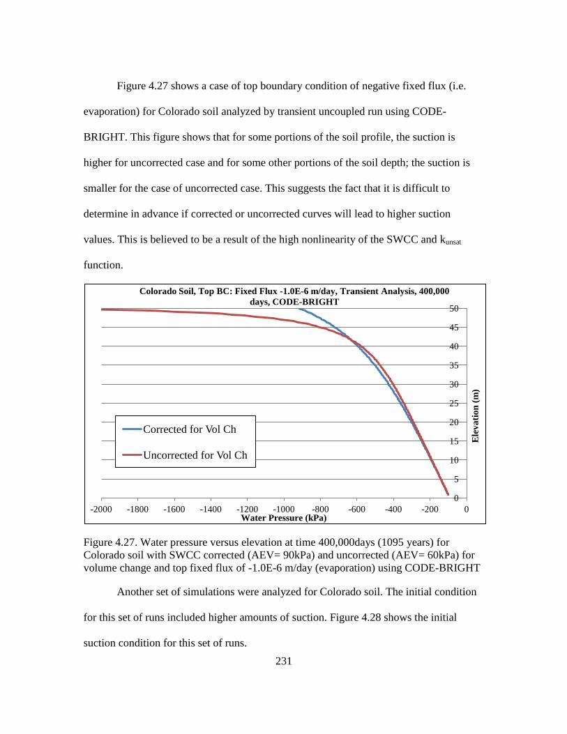
231
Figure 4.27 shows a case of top boundary condition of negative fixed flux (i.e.
evaporation) for Colorado soil analyzed by transient uncoupled run using CODE-
BRIGHT. This figure shows that for some portions of the soil profile, the suction is
higher for uncorrected case and for some other portions of the soil depth; the suction is
smaller for the case of uncorrected case. This suggests the fact that it is difficult to
determine in advance if corrected or uncorrected curves will lead to higher suction
values. This is believed to be a result of the high nonlinearity of the SWCC and kunsat
function.
Figure 4.27. Water pressure versus elevation at time 400,000days (1095 years) for
Colorado soil with SWCC corrected (AEV= 90kPa) and uncorrected (AEV= 60kPa) for
volume change and top fixed flux of -1.0E-6 m/day (evaporation) using CODE-BRIGHT
Another set of simulations were analyzed for Colorado soil. The initial condition
for this set of runs included higher amounts of suction. Figure 4.28 shows the initial
suction condition for this set of runs.
0
5
10
15
20
25
30
35
40
45
50
-2000 -1800 -1600 -1400 -1200 -1000 -800 -600 -400 -200 0
Ele
va
tio
n (
m)
Water Pressure (kPa)
Colorado Soil, Top BC: Fixed Flux -1.0E-6 m/day, Transient Analysis, 400,000
days, CODE-BRIGHT
Corrected for Vol Ch
Uncorrected for Vol Ch
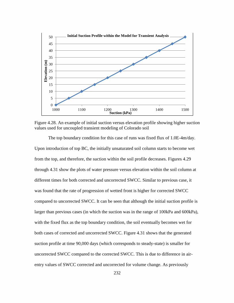
232
Figure 4.28. An example of initial suction versus elevation profile showing higher suction
values used for uncoupled transient modeling of Colorado soil
The top boundary condition for this case of runs was fixed flux of 1.0E-4m/day.
Upon introduction of top BC, the initially unsaturated soil column starts to become wet
from the top, and therefore, the suction within the soil profile decreases. Figures 4.29
through 4.31 show the plots of water pressure versus elevation within the soil column at
different times for both corrected and uncorrected SWCC. Similar to previous case, it
was found that the rate of progression of wetted front is higher for corrected SWCC
compared to uncorrected SWCC. It can be seen that although the initial suction profile is
larger than previous cases (in which the suction was in the range of 100kPa and 600kPa),
with the fixed flux as the top boundary condition, the soil eventually becomes wet for
both cases of corrected and uncorrected SWCC. Figure 4.31 shows that the generated
suction profile at time 90,000 days (which corresponds to steady-state) is smaller for
uncorrected SWCC compared to the corrected SWCC. This is due to difference in air-
entry values of SWCC corrected and uncorrected for volume change. As previously
0
5
10
15
20
25
30
35
40
45
50
1000 1100 1200 1300 1400 1500
Ele
va
tio
n (
m)
Suction (kPa)
Initial Suction Profile within the Model for Transient Analysis
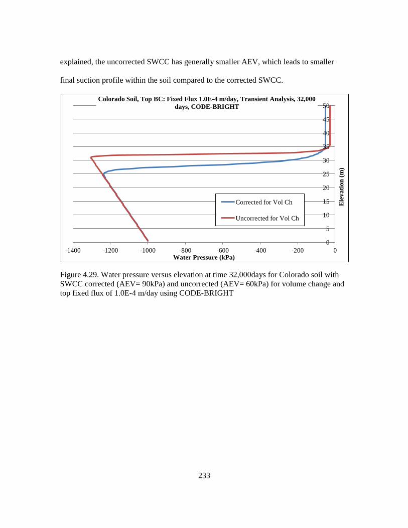
233
explained, the uncorrected SWCC has generally smaller AEV, which leads to smaller
final suction profile within the soil compared to the corrected SWCC.
Figure 4.29. Water pressure versus elevation at time 32,000days for Colorado soil with
SWCC corrected (AEV= 90kPa) and uncorrected (AEV= 60kPa) for volume change and
top fixed flux of 1.0E-4 m/day using CODE-BRIGHT
0
5
10
15
20
25
30
35
40
45
50
-1400 -1200 -1000 -800 -600 -400 -200 0
Ele
va
tio
n (
m)
Water Pressure (kPa)
Colorado Soil, Top BC: Fixed Flux 1.0E-4 m/day, Transient Analysis, 32,000
days, CODE-BRIGHT
Corrected for Vol Ch
Uncorrected for Vol Ch
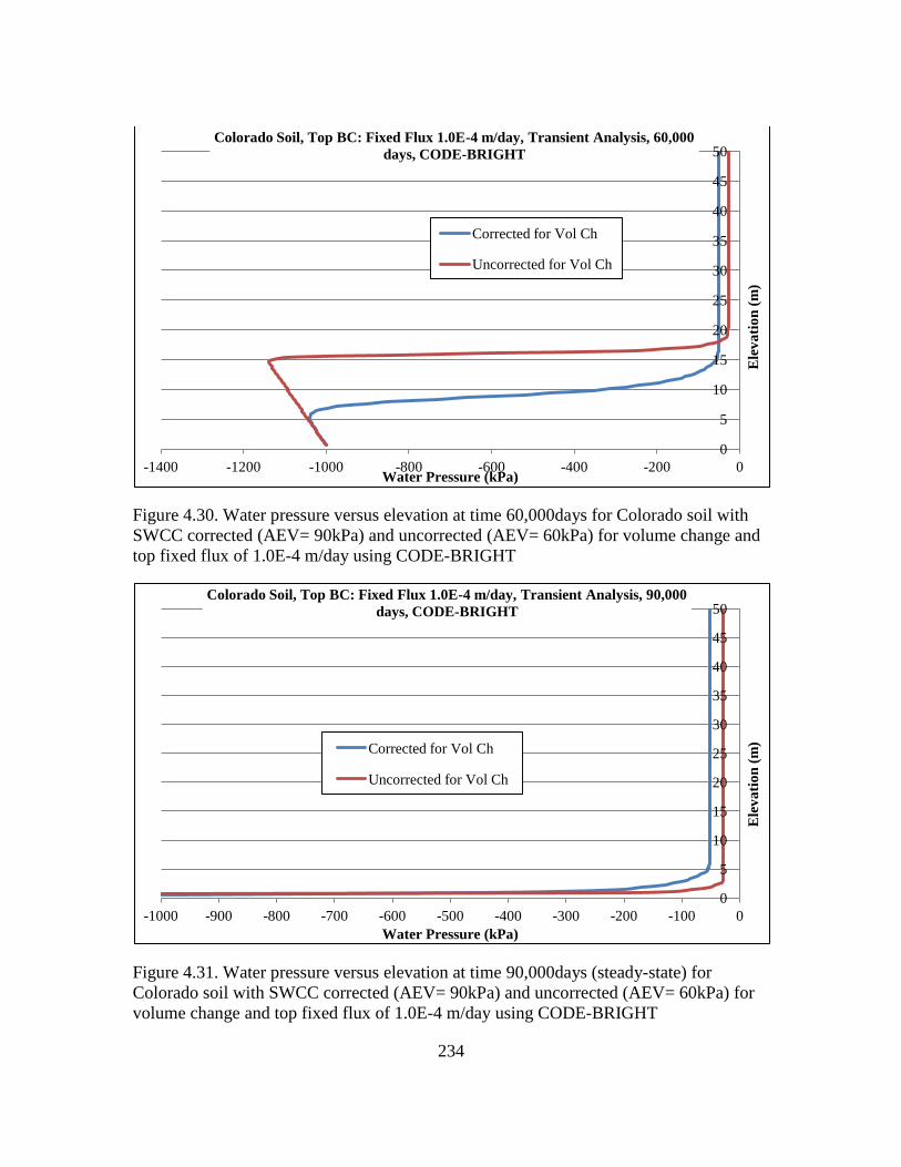
234
Figure 4.30. Water pressure versus elevation at time 60,000days for Colorado soil with
SWCC corrected (AEV= 90kPa) and uncorrected (AEV= 60kPa) for volume change and
top fixed flux of 1.0E-4 m/day using CODE-BRIGHT
Figure 4.31. Water pressure versus elevation at time 90,000days (steady-state) for
Colorado soil with SWCC corrected (AEV= 90kPa) and uncorrected (AEV= 60kPa) for
volume change and top fixed flux of 1.0E-4 m/day using CODE-BRIGHT
0
5
10
15
20
25
30
35
40
45
50
-1400 -1200 -1000 -800 -600 -400 -200 0
Ele
va
tio
n (
m)
Water Pressure (kPa)
Colorado Soil, Top BC: Fixed Flux 1.0E-4 m/day, Transient Analysis, 60,000
days, CODE-BRIGHT
Corrected for Vol Ch
Uncorrected for Vol Ch
0
5
10
15
20
25
30
35
40
45
50
-1000 -900 -800 -700 -600 -500 -400 -300 -200 -100 0
Ele
va
tio
n (
m)
Water Pressure (kPa)
Colorado Soil, Top BC: Fixed Flux 1.0E-4 m/day, Transient Analysis, 90,000
days, CODE-BRIGHT
Corrected for Vol Ch
Uncorrected for Vol Ch

235
4.10.1.3. San Antonio Soil
Table 4.9 provides a list of numerical modeling conducted based on properties of
San Antonio soil. Figures 4.32 through 4.36 show results of modeling using San Antonio
soil. Similar result trends to Anthem, and Colorado soils were found for San Antonio soil.
At time 15,000 days which is a long-enough time for the model to reach the steady-state
(i.e. the soil profile has become wetted), in the model based on uncorrected SWCC the
final suction throughout the soil column is smaller than the final suction of the model
based on corrected SWCC (suction of 8kPa for uncorrected SWCC versus 18kPa for
corrected SWCC for the majority of the soil profile). In addition, the rate of progression
of wetted front is larger for the case of SWCC corrected for volume change due to higher
unsaturated hydraulic conductivity. This leads to higher suctions for uncorrected SWCC
at some points within the soil profile at times prior to 15,000 days. This is shown in
Figures 4.34 and 4.35 in which at times 6,000 days and 10,000 days, in some portions of
the soil depth the uncorrected SWCC shows higher suction values compared to suctions
of corrected SWCC. This is due to the fact that at times 6,000 days and 10,000 days the
depth of wetting is larger for volume-corrected SWCC.
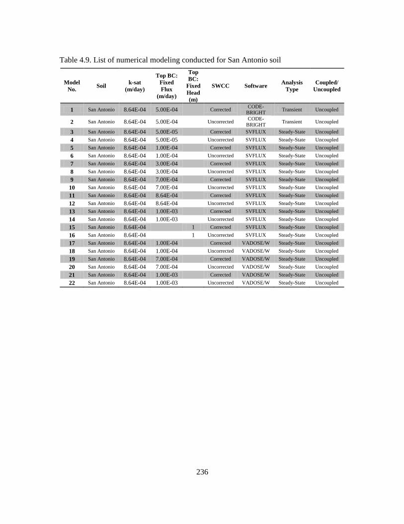
236
Table 4.9. List of numerical modeling conducted for San Antonio soil
Model
No. Soil
k-sat
(m/day)
Top BC:
Fixed
Flux
(m/day)
Top
BC:
Fixed
Head
(m)
SWCC Software Analysis
Type
Coupled/
Uncoupled
1 San Antonio 8.64E-04 5.00E-04
Corrected CODE-
BRIGHT Transient Uncoupled
2 San Antonio 8.64E-04 5.00E-04
Uncorrected CODE-
BRIGHT Transient Uncoupled
3 San Antonio 8.64E-04 5.00E-05
Corrected SVFLUX Steady-State Uncoupled
4 San Antonio 8.64E-04 5.00E-05
Uncorrected SVFLUX Steady-State Uncoupled
5 San Antonio 8.64E-04 1.00E-04
Corrected SVFLUX Steady-State Uncoupled
6 San Antonio 8.64E-04 1.00E-04
Uncorrected SVFLUX Steady-State Uncoupled
7 San Antonio 8.64E-04 3.00E-04
Corrected SVFLUX Steady-State Uncoupled
8 San Antonio 8.64E-04 3.00E-04
Uncorrected SVFLUX Steady-State Uncoupled
9 San Antonio 8.64E-04 7.00E-04
Corrected SVFLUX Steady-State Uncoupled
10 San Antonio 8.64E-04 7.00E-04
Uncorrected SVFLUX Steady-State Uncoupled
11 San Antonio 8.64E-04 8.64E-04
Corrected SVFLUX Steady-State Uncoupled
12 San Antonio 8.64E-04 8.64E-04
Uncorrected SVFLUX Steady-State Uncoupled
13 San Antonio 8.64E-04 1.00E-03
Corrected SVFLUX Steady-State Uncoupled
14 San Antonio 8.64E-04 1.00E-03
Uncorrected SVFLUX Steady-State Uncoupled
15 San Antonio 8.64E-04
1 Corrected SVFLUX Steady-State Uncoupled
16 San Antonio 8.64E-04
1 Uncorrected SVFLUX Steady-State Uncoupled
17 San Antonio 8.64E-04 1.00E-04
Corrected VADOSE/W Steady-State Uncoupled
18 San Antonio 8.64E-04 1.00E-04
Uncorrected VADOSE/W Steady-State Uncoupled
19 San Antonio 8.64E-04 7.00E-04
Corrected VADOSE/W Steady-State Uncoupled
20 San Antonio 8.64E-04 7.00E-04
Uncorrected VADOSE/W Steady-State Uncoupled
21 San Antonio 8.64E-04 1.00E-03
Corrected VADOSE/W Steady-State Uncoupled
22 San Antonio 8.64E-04 1.00E-03
Uncorrected VADOSE/W Steady-State Uncoupled
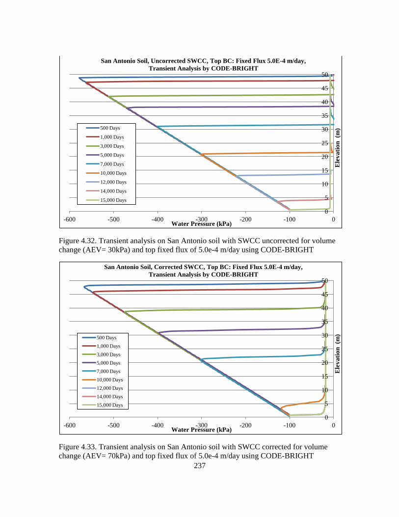
237
Figure 4.32. Transient analysis on San Antonio soil with SWCC uncorrected for volume
change (AEV= 30kPa) and top fixed flux of 5.0e-4 m/day using CODE-BRIGHT
Figure 4.33. Transient analysis on San Antonio soil with SWCC corrected for volume
change (AEV= 70kPa) and top fixed flux of 5.0e-4 m/day using CODE-BRIGHT
0
5
10
15
20
25
30
35
40
45
50
-600 -500 -400 -300 -200 -100 0
Ele
va
tio
n (m
)
Water Pressure (kPa)
San Antonio Soil, Uncorrected SWCC, Top BC: Fixed Flux 5.0E-4 m/day,
Transient Analysis by CODE-BRIGHT
500 Days
1,000 Days
3,000 Days
5,000 Days
7,000 Days
10,000 Days
12,000 Days
14,000 Days
15,000 Days
0
5
10
15
20
25
30
35
40
45
50
-600 -500 -400 -300 -200 -100 0
Ele
va
tio
n (m
)
Water Pressure (kPa)
San Antonio Soil, Corrected SWCC, Top BC: Fixed Flux 5.0E-4 m/day,
Transient Analysis by CODE-BRIGHT
500 Days
1,000 Days
3,000 Days
5,000 Days
7,000 Days
10,000 Days
12,000 Days
14,000 Days
15,000 Days

238
Figure 4.34. Water pressure versus elevation at time 6,000 days (16 years) for San
Antonio soil with SWCC corrected (AEV= 70kPa) and uncorrected (AEV= 30kPa) for
volume change and top fixed flux of 5.0e-4 m/day using CODE-BRIGHT
Figure 4.35. Water pressure versus elevation at time 10,000 days (27 years) for San
Antonio soil with SWCC corrected (AEV= 70kPa) and uncorrected (AEV= 30kPa) for
volume change and top fixed flux of 5.0e-4 m/day using CODE-BRIGHT
0
5
10
15
20
25
30
35
40
45
50
-600 -500 -400 -300 -200 -100 0
Ele
va
tio
n (
m)
Water Pressure (kPa)
San Antonio Soil, Top BC: Fixed Flux 5.0E-4 m/day, 6,000 Days, CODE-
BRIGHT
Corrected for Vol Ch
Uncorrected for Vol Ch
0
5
10
15
20
25
30
35
40
45
50
-600 -500 -400 -300 -200 -100 0
Ele
va
tio
n (
m)
Water Pressure (kPa)
San Antonio Soil, Top BC: Fixed Flux 5.0E-4 m/day, 10,000 Days, CODE-
BRIGHT
Corrected for Vol Ch
Uncorrected for Vol Ch
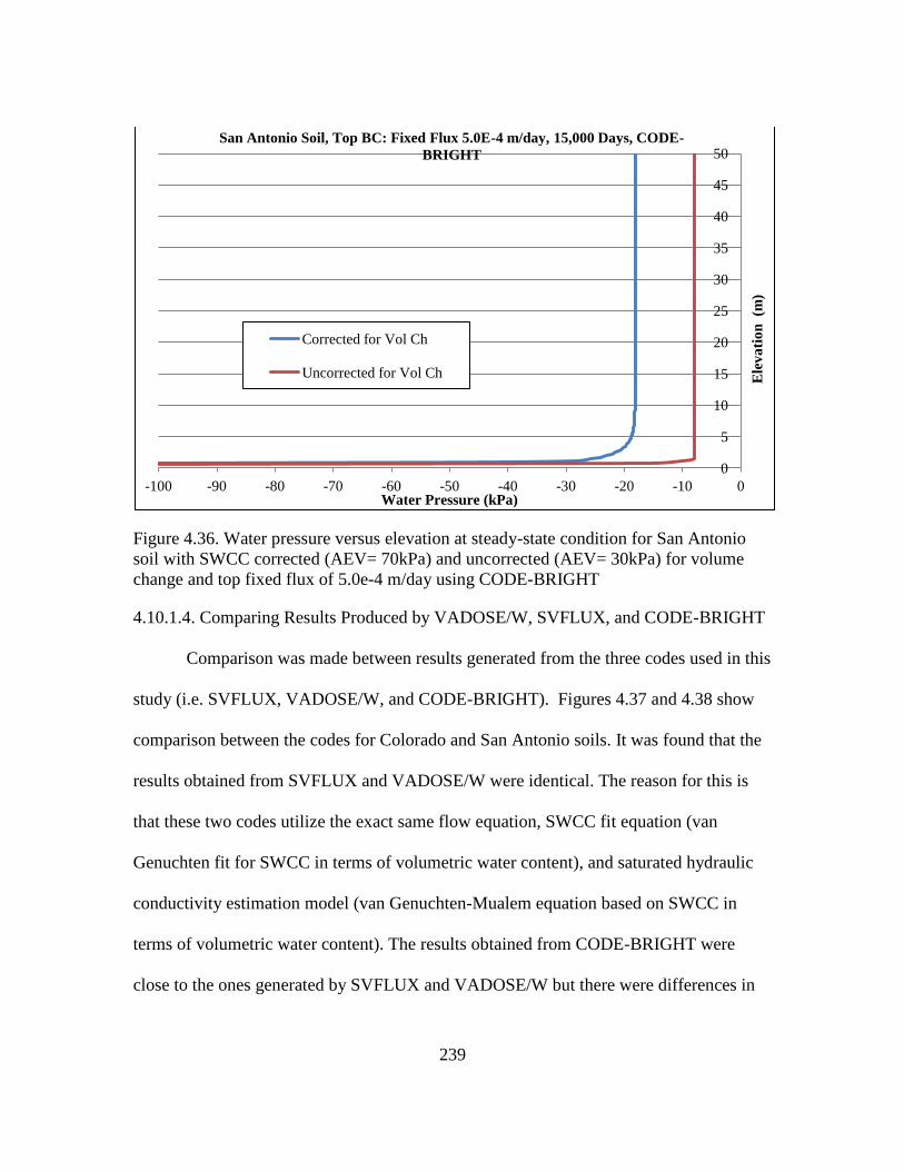
239
Figure 4.36. Water pressure versus elevation at steady-state condition for San Antonio
soil with SWCC corrected (AEV= 70kPa) and uncorrected (AEV= 30kPa) for volume
change and top fixed flux of 5.0e-4 m/day using CODE-BRIGHT
4.10.1.4. Comparing Results Produced by VADOSE/W, SVFLUX, and CODE-BRIGHT
Comparison was made between results generated from the three codes used in this
study (i.e. SVFLUX, VADOSE/W, and CODE-BRIGHT). Figures 4.37 and 4.38 show
comparison between the codes for Colorado and San Antonio soils. It was found that the
results obtained from SVFLUX and VADOSE/W were identical. The reason for this is
that these two codes utilize the exact same flow equation, SWCC fit equation (van
Genuchten fit for SWCC in terms of volumetric water content), and saturated hydraulic
conductivity estimation model (van Genuchten-Mualem equation based on SWCC in
terms of volumetric water content). The results obtained from CODE-BRIGHT were
close to the ones generated by SVFLUX and VADOSE/W but there were differences in
0
5
10
15
20
25
30
35
40
45
50
-100 -90 -80 -70 -60 -50 -40 -30 -20 -10 0
Ele
va
tio
n (m
)
Water Pressure (kPa)
San Antonio Soil, Top BC: Fixed Flux 5.0E-4 m/day, 15,000 Days, CODE-
BRIGHT
Corrected for Vol Ch
Uncorrected for Vol Ch
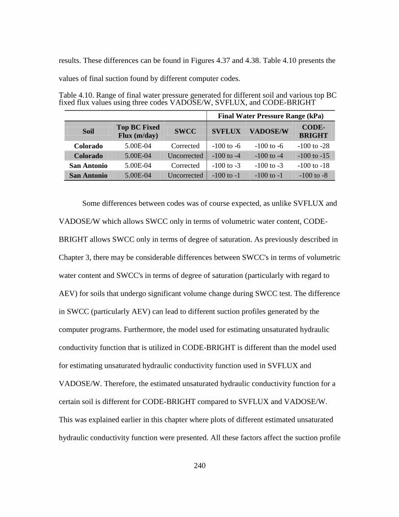
240
results. These differences can be found in Figures 4.37 and 4.38. Table 4.10 presents the
values of final suction found by different computer codes.
Table 4.10. Range of final water pressure generated for different soil and various top BC fixed flux values using three codes VADOSE/W, SVFLUX, and CODE-BRIGHT
Final Water Pressure Range (kPa)
Soil Top BC Fixed
Flux (m/day) SWCC SVFLUX VADOSE/W
CODE-
BRIGHT
Colorado 5.00E-04 Corrected -100 to -6 -100 to -6 -100 to -28
Colorado 5.00E-04 Uncorrected -100 to -4 -100 to -4 -100 to -15
San Antonio 5.00E-04 Corrected -100 to -3 -100 to -3 -100 to -18
San Antonio 5.00E-04 Uncorrected -100 to -1 -100 to -1 -100 to -8
Some differences between codes was of course expected, as unlike SVFLUX and
VADOSE/W which allows SWCC only in terms of volumetric water content, CODE-
BRIGHT allows SWCC only in terms of degree of saturation. As previously described in
Chapter 3, there may be considerable differences between SWCC's in terms of volumetric
water content and SWCC's in terms of degree of saturation (particularly with regard to
AEV) for soils that undergo significant volume change during SWCC test. The difference
in SWCC (particularly AEV) can lead to different suction profiles generated by the
computer programs. Furthermore, the model used for estimating unsaturated hydraulic
conductivity function that is utilized in CODE-BRIGHT is different than the model used
for estimating unsaturated hydraulic conductivity function used in SVFLUX and
VADOSE/W. Therefore, the estimated unsaturated hydraulic conductivity function for a
certain soil is different for CODE-BRIGHT compared to SVFLUX and VADOSE/W.
This was explained earlier in this chapter where plots of different estimated unsaturated
hydraulic conductivity function were presented. All these factors affect the suction profile
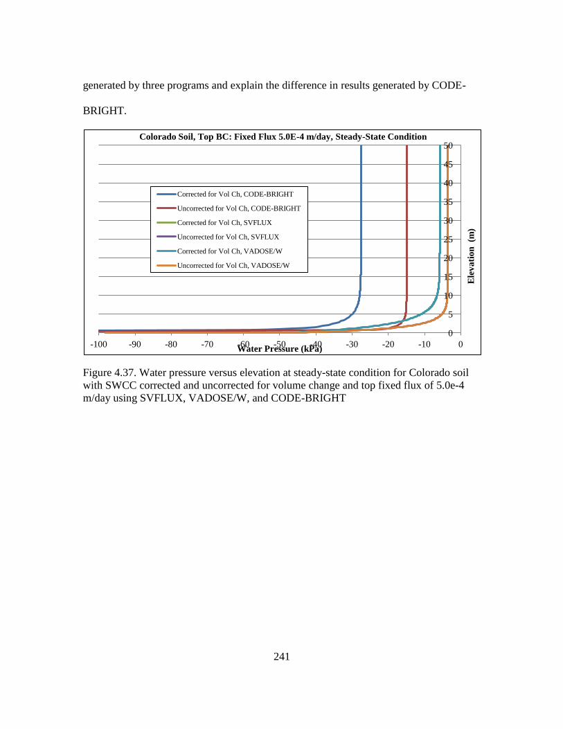
241
generated by three programs and explain the difference in results generated by CODE-
BRIGHT.
Figure 4.37. Water pressure versus elevation at steady-state condition for Colorado soil
with SWCC corrected and uncorrected for volume change and top fixed flux of 5.0e-4
m/day using SVFLUX, VADOSE/W, and CODE-BRIGHT
0
5
10
15
20
25
30
35
40
45
50
-100 -90 -80 -70 -60 -50 -40 -30 -20 -10 0
Ele
va
tio
n (m
)
Water Pressure (kPa)
Colorado Soil, Top BC: Fixed Flux 5.0E-4 m/day, Steady-State Condition
Corrected for Vol Ch, CODE-BRIGHT
Uncorrected for Vol Ch, CODE-BRIGHT
Corrected for Vol Ch, SVFLUX
Uncorrected for Vol Ch, SVFLUX
Corrected for Vol Ch, VADOSE/W
Uncorrected for Vol Ch, VADOSE/W
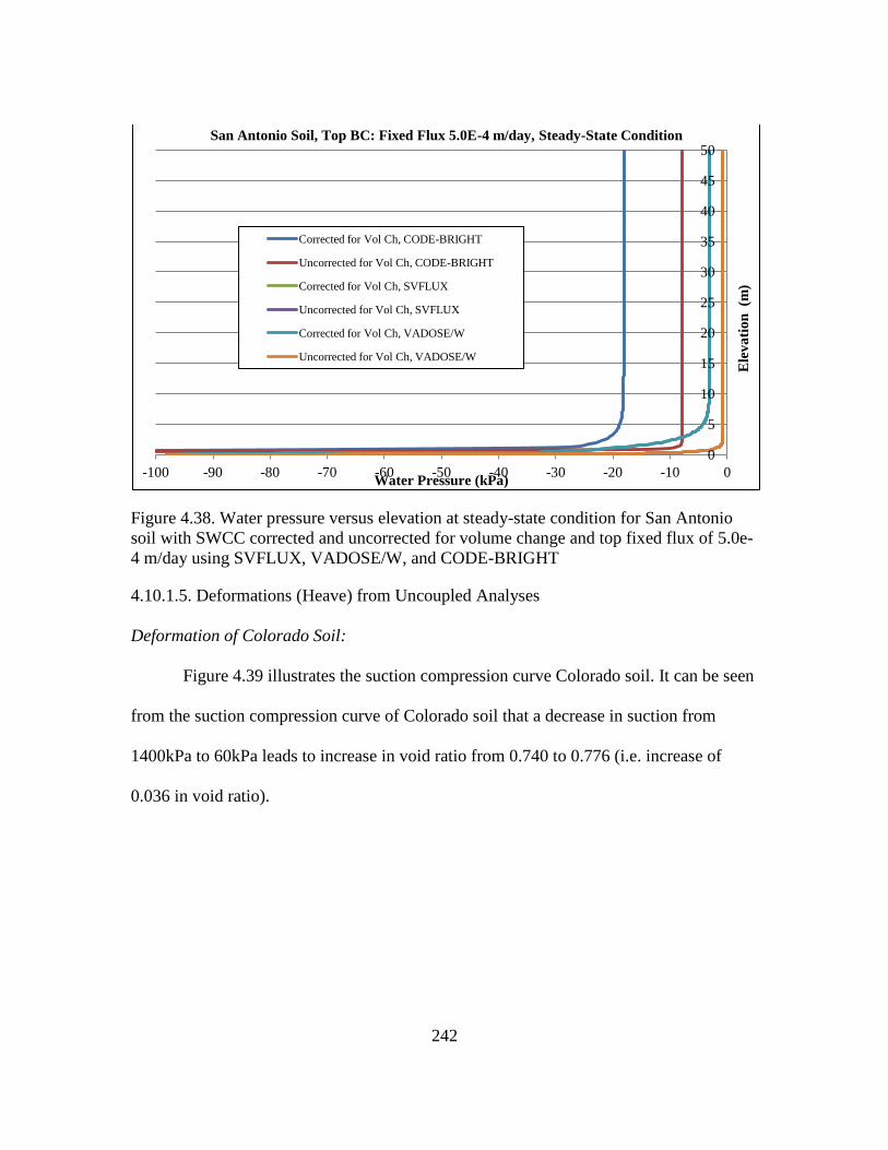
242
Figure 4.38. Water pressure versus elevation at steady-state condition for San Antonio
soil with SWCC corrected and uncorrected for volume change and top fixed flux of 5.0e-
4 m/day using SVFLUX, VADOSE/W, and CODE-BRIGHT
4.10.1.5. Deformations (Heave) from Uncoupled Analyses
Deformation of Colorado Soil:
Figure 4.39 illustrates the suction compression curve Colorado soil. It can be seen
from the suction compression curve of Colorado soil that a decrease in suction from
1400kPa to 60kPa leads to increase in void ratio from 0.740 to 0.776 (i.e. increase of
0.036 in void ratio).
0
5
10
15
20
25
30
35
40
45
50
-100 -90 -80 -70 -60 -50 -40 -30 -20 -10 0
Ele
va
tio
n (m
)
Water Pressure (kPa)
San Antonio Soil, Top BC: Fixed Flux 5.0E-4 m/day, Steady-State Condition
Corrected for Vol Ch, CODE-BRIGHT
Uncorrected for Vol Ch, CODE-BRIGHT
Corrected for Vol Ch, SVFLUX
Uncorrected for Vol Ch, SVFLUX
Corrected for Vol Ch, VADOSE/W
Uncorrected for Vol Ch, VADOSE/W
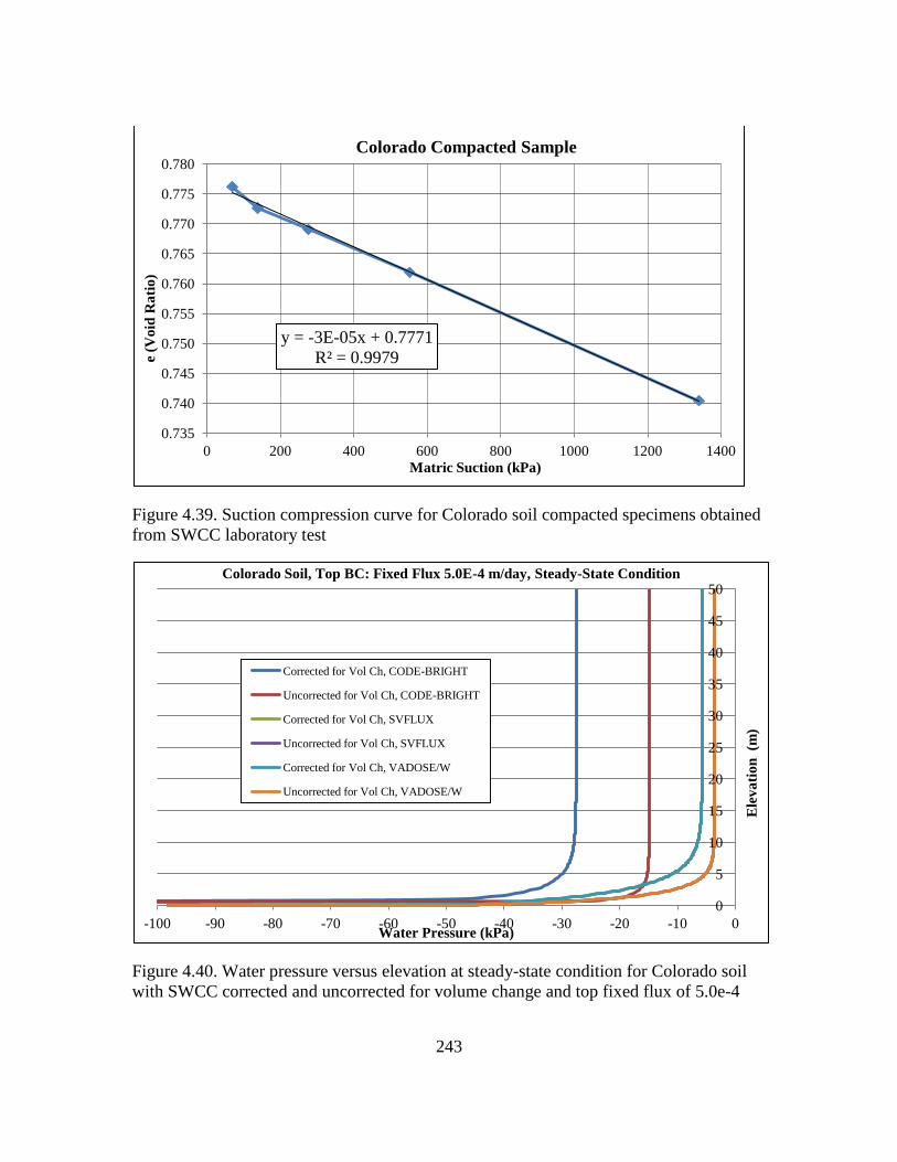
243
Figure 4.39. Suction compression curve for Colorado soil compacted specimens obtained
from SWCC laboratory test
Figure 4.40. Water pressure versus elevation at steady-state condition for Colorado soil
with SWCC corrected and uncorrected for volume change and top fixed flux of 5.0e-4
y = -3E-05x + 0.7771
R² = 0.9979
0.735
0.740
0.745
0.750
0.755
0.760
0.765
0.770
0.775
0.780
0 200 400 600 800 1000 1200 1400
e (V
oid
Ra
tio
)
Matric Suction (kPa)
Colorado Compacted Sample
0
5
10
15
20
25
30
35
40
45
50
-100 -90 -80 -70 -60 -50 -40 -30 -20 -10 0
Ele
va
tio
n (m
)
Water Pressure (kPa)
Colorado Soil, Top BC: Fixed Flux 5.0E-4 m/day, Steady-State Condition
Corrected for Vol Ch, CODE-BRIGHT
Uncorrected for Vol Ch, CODE-BRIGHT
Corrected for Vol Ch, SVFLUX
Uncorrected for Vol Ch, SVFLUX
Corrected for Vol Ch, VADOSE/W
Uncorrected for Vol Ch, VADOSE/W
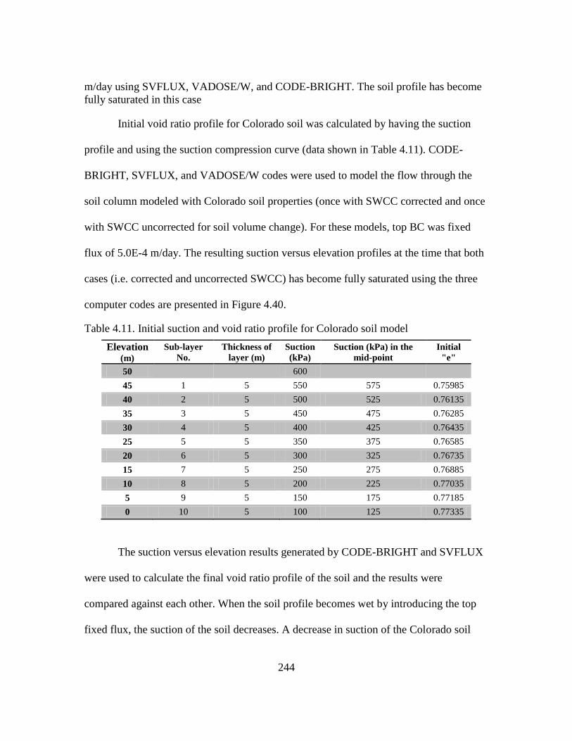
244
m/day using SVFLUX, VADOSE/W, and CODE-BRIGHT. The soil profile has become
fully saturated in this case
Initial void ratio profile for Colorado soil was calculated by having the suction
profile and using the suction compression curve (data shown in Table 4.11). CODE-
BRIGHT, SVFLUX, and VADOSE/W codes were used to model the flow through the
soil column modeled with Colorado soil properties (once with SWCC corrected and once
with SWCC uncorrected for soil volume change). For these models, top BC was fixed
flux of 5.0E-4 m/day. The resulting suction versus elevation profiles at the time that both
cases (i.e. corrected and uncorrected SWCC) has become fully saturated using the three
computer codes are presented in Figure 4.40.
Table 4.11. Initial suction and void ratio profile for Colorado soil model
Elevation (m)
Sub-layer
No.
Thickness of
layer (m)
Suction
(kPa)
Suction (kPa) in the
mid-point
Initial
"e"
50
600
45 1 5 550 575 0.75985
40 2 5 500 525 0.76135
35 3 5 450 475 0.76285
30 4 5 400 425 0.76435
25 5 5 350 375 0.76585
20 6 5 300 325 0.76735
15 7 5 250 275 0.76885
10 8 5 200 225 0.77035
5 9 5 150 175 0.77185
0 10 5 100 125 0.77335
The suction versus elevation results generated by CODE-BRIGHT and SVFLUX
were used to calculate the final void ratio profile of the soil and the results were
compared against each other. When the soil profile becomes wet by introducing the top
fixed flux, the suction of the soil decreases. A decrease in suction of the Colorado soil
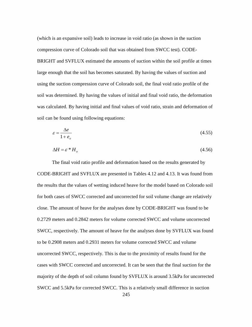
245
(which is an expansive soil) leads to increase in void ratio (as shown in the suction
compression curve of Colorado soil that was obtained from SWCC test). CODE-
BRIGHT and SVFLUX estimated the amounts of suction within the soil profile at times
large enough that the soil has becomes saturated. By having the values of suction and
using the suction compression curve of Colorado soil, the final void ratio profile of the
soil was determined. By having the values of initial and final void ratio, the deformation
was calculated. By having initial and final values of void ratio, strain and deformation of
soil can be found using following equations:
oe
e
1 (4.55)
oHH * (4.56)
The final void ratio profile and deformation based on the results generated by
CODE-BRIGHT and SVFLUX are presented in Tables 4.12 and 4.13. It was found from
the results that the values of wetting induced heave for the model based on Colorado soil
for both cases of SWCC corrected and uncorrected for soil volume change are relatively
close. The amount of heave for the analyses done by CODE-BRIGHT was found to be
0.2729 meters and 0.2842 meters for volume corrected SWCC and volume uncorrected
SWCC, respectively. The amount of heave for the analyses done by SVFLUX was found
to be 0.2908 meters and 0.2931 meters for volume corrected SWCC and volume
uncorrected SWCC, respectively. This is due to the proximity of results found for the
cases with SWCC corrected and uncorrected. It can be seen that the final suction for the
majority of the depth of soil column found by SVFLUX is around 3.5kPa for uncorrected
SWCC and 5.5kPa for corrected SWCC. This is a relatively small difference in suction
246
which leads to small differences in void ratios calculated based on suction (i.e. from the
suction compression curve). However, this difference in the results obtained from the
analyses done by CODE-BRIGHT is more pronounced compared to the difference in
deformation values found from the results of runs by SVFLUX. It can be seen from
Figure 4.40 that the suction generated by CODE-BRIGHT for the majority of soil depth
for uncorrected SWCC is around 15kPa while this value is around 28kPa for corrected
SWCC. This difference in final suction values between corrected and uncorrected SWCC
is more pronounced than this difference in results of SVFLUX. This leads to more
pronounced differences in calculated void ratio and deformation for corrected and
uncorrected SWCC analyzed by CODE-BRIGHT.
It was also found that the deformation determined form SVFLUX results were
slightly larger than the ones calculated from CODE-BRIGHT results. This is due to the
fact that the final suction profile (for both SWCC corrected and uncorrected) generated
by SVFLUX are smaller than the values generated by CODE-BRIGHT. This leads to
relatively larger void ratios calculated by using the suction compression curve.
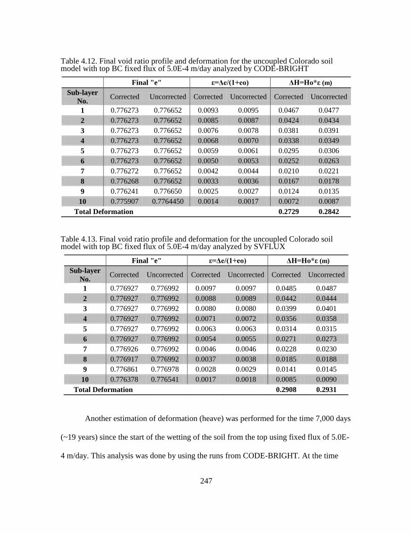
247
Table 4.12. Final void ratio profile and deformation for the uncoupled Colorado soil model with top BC fixed flux of 5.0E-4 m/day analyzed by CODE-BRIGHT
Final "e" ε=Δe/(1+eo) ΔH=Ho*ε (m)
Sub-layer
No. Corrected Uncorrected Corrected Uncorrected Corrected Uncorrected
1 0.776273 0.776652 0.0093 0.0095 0.0467 0.0477
2 0.776273 0.776652 0.0085 0.0087 0.0424 0.0434
3 0.776273 0.776652 0.0076 0.0078 0.0381 0.0391
4 0.776273 0.776652 0.0068 0.0070 0.0338 0.0349
5 0.776273 0.776652 0.0059 0.0061 0.0295 0.0306
6 0.776273 0.776652 0.0050 0.0053 0.0252 0.0263
7 0.776272 0.776652 0.0042 0.0044 0.0210 0.0221
8 0.776268 0.776652 0.0033 0.0036 0.0167 0.0178
9 0.776241 0.776650 0.0025 0.0027 0.0124 0.0135
10 0.775907 0.7764450 0.0014 0.0017 0.0072 0.0087
Total Deformation
0.2729 0.2842
Table 4.13. Final void ratio profile and deformation for the uncoupled Colorado soil model with top BC fixed flux of 5.0E-4 m/day analyzed by SVFLUX
Final "e" ε=Δe/(1+eo) ΔH=Ho*ε (m)
Sub-layer
No. Corrected Uncorrected Corrected Uncorrected Corrected Uncorrected
1 0.776927 0.776992 0.0097 0.0097 0.0485 0.0487
2 0.776927 0.776992 0.0088 0.0089 0.0442 0.0444
3 0.776927 0.776992 0.0080 0.0080 0.0399 0.0401
4 0.776927 0.776992 0.0071 0.0072 0.0356 0.0358
5 0.776927 0.776992 0.0063 0.0063 0.0314 0.0315
6 0.776927 0.776992 0.0054 0.0055 0.0271 0.0273
7 0.776926 0.776992 0.0046 0.0046 0.0228 0.0230
8 0.776917 0.776992 0.0037 0.0038 0.0185 0.0188
9 0.776861 0.776978 0.0028 0.0029 0.0141 0.0145
10 0.776378 0.776541 0.0017 0.0018 0.0085 0.0090
Total Deformation
0.2908 0.2931
Another estimation of deformation (heave) was performed for the time 7,000 days
(~19 years) since the start of the wetting of the soil from the top using fixed flux of 5.0E-
4 m/day. This analysis was done by using the runs from CODE-BRIGHT. At the time
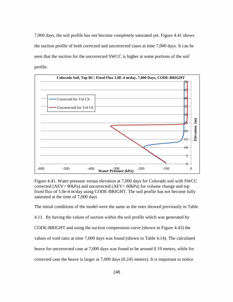
248
7,000 days, the soil profile has not become completely saturated yet. Figure 4.41 shows
the suction profile of both corrected and uncorrected cases at time 7,000 days. It can be
seen that the suction for the uncorrected SWCC is higher at some portions of the soil
profile.
Figure 4.41. Water pressure versus elevation at 7,000 days for Colorado soil with SWCC
corrected (AEV= 90kPa) and uncorrected (AEV= 60kPa) for volume change and top
fixed flux of 5.0e-4 m/day using CODE-BRIGHT. The soil profile has not become fully
saturated at the time of 7,000 days
The initial conditions of the model were the same as the ones showed previously in Table
4.11. By having the values of suction within the soil profile which was generated by
CODE-BRIGHT and using the suction compression curve (shown in Figure 4.43) the
values of void ratio at time 7,000 days was found (shown in Table 4.14). The calculated
heave for uncorrected case at 7,000 days was found to be around 0.19 meters, while for
corrected case the heave is larger at 7,000 days (0.245 meters). It is important to notice
0
5
10
15
20
25
30
35
40
45
50
-600 -500 -400 -300 -200 -100 0
Ele
va
tio
n (m
)
Water Pressure (kPa)
Colorado Soil, Top BC: Fixed Flux 5.0E-4 m/day, 7,000 Days, CODE-BRIGHT
Corrected for Vol Ch
Uncorrected for Vol Ch
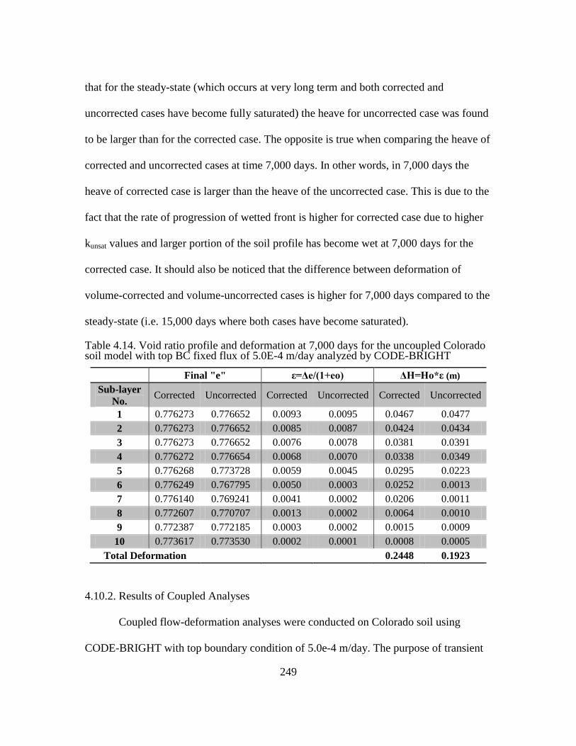
249
that for the steady-state (which occurs at very long term and both corrected and
uncorrected cases have become fully saturated) the heave for uncorrected case was found
to be larger than for the corrected case. The opposite is true when comparing the heave of
corrected and uncorrected cases at time 7,000 days. In other words, in 7,000 days the
heave of corrected case is larger than the heave of the uncorrected case. This is due to the
fact that the rate of progression of wetted front is higher for corrected case due to higher
kunsat values and larger portion of the soil profile has become wet at 7,000 days for the
corrected case. It should also be noticed that the difference between deformation of
volume-corrected and volume-uncorrected cases is higher for 7,000 days compared to the
steady-state (i.e. 15,000 days where both cases have become saturated).
Table 4.14. Void ratio profile and deformation at 7,000 days for the uncoupled Colorado soil model with top BC fixed flux of 5.0E-4 m/day analyzed by CODE-BRIGHT
Final "e" ε=Δe/(1+eo) ΔH=Ho*ε (m)
Sub-layer
No. Corrected Uncorrected Corrected Uncorrected Corrected Uncorrected
1 0.776273 0.776652 0.0093 0.0095 0.0467 0.0477
2 0.776273 0.776652 0.0085 0.0087 0.0424 0.0434
3 0.776273 0.776652 0.0076 0.0078 0.0381 0.0391
4 0.776272 0.776654 0.0068 0.0070 0.0338 0.0349
5 0.776268 0.773728 0.0059 0.0045 0.0295 0.0223
6 0.776249 0.767795 0.0050 0.0003 0.0252 0.0013
7 0.776140 0.769241 0.0041 0.0002 0.0206 0.0011
8 0.772607 0.770707 0.0013 0.0002 0.0064 0.0010
9 0.772387 0.772185 0.0003 0.0002 0.0015 0.0009
10 0.773617 0.773530 0.0002 0.0001 0.0008 0.0005
Total Deformation
0.2448 0.1923
4.10.2. Results of Coupled Analyses
Coupled flow-deformation analyses were conducted on Colorado soil using
CODE-BRIGHT with top boundary condition of 5.0e-4 m/day. The purpose of transient
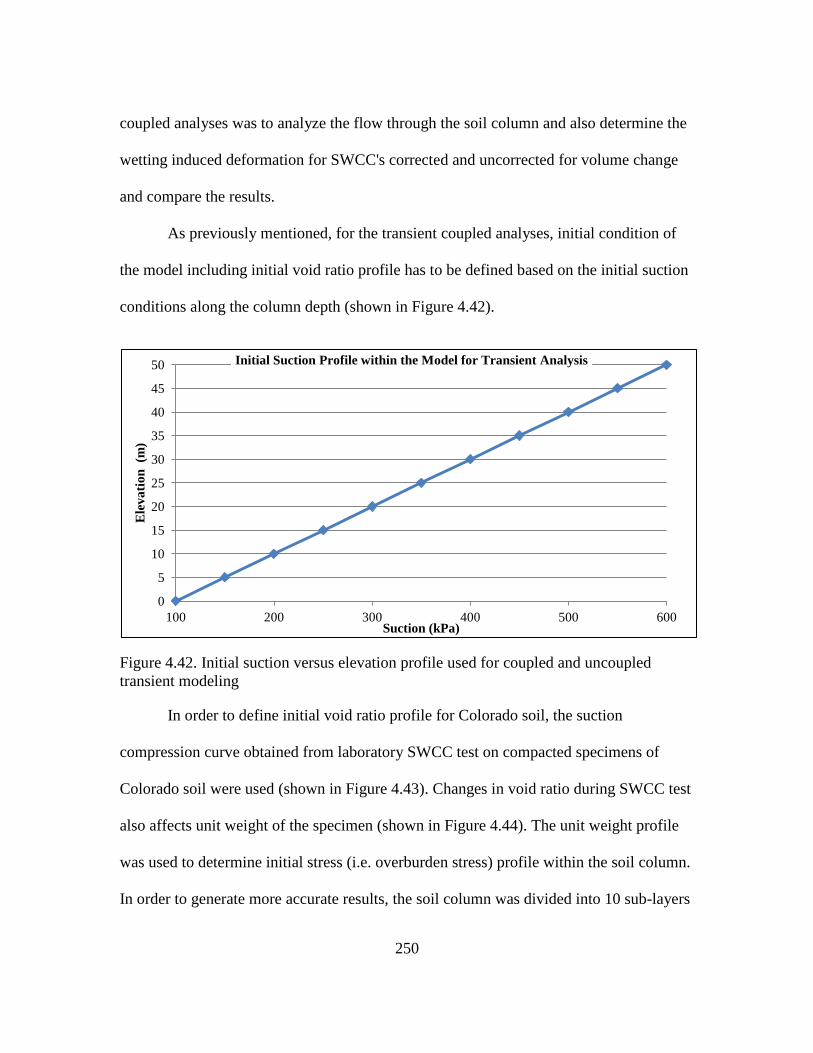
250
coupled analyses was to analyze the flow through the soil column and also determine the
wetting induced deformation for SWCC's corrected and uncorrected for volume change
and compare the results.
As previously mentioned, for the transient coupled analyses, initial condition of
the model including initial void ratio profile has to be defined based on the initial suction
conditions along the column depth (shown in Figure 4.42).
Figure 4.42. Initial suction versus elevation profile used for coupled and uncoupled
transient modeling
In order to define initial void ratio profile for Colorado soil, the suction
compression curve obtained from laboratory SWCC test on compacted specimens of
Colorado soil were used (shown in Figure 4.43). Changes in void ratio during SWCC test
also affects unit weight of the specimen (shown in Figure 4.44). The unit weight profile
was used to determine initial stress (i.e. overburden stress) profile within the soil column.
In order to generate more accurate results, the soil column was divided into 10 sub-layers
0
5
10
15
20
25
30
35
40
45
50
100 200 300 400 500 600
Ele
va
tio
n (m
)
Suction (kPa)
Initial Suction Profile within the Model for Transient Analysis
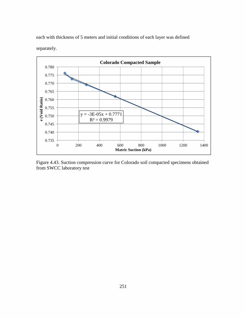
251
each with thickness of 5 meters and initial conditions of each layer was defined
separately.
Figure 4.43. Suction compression curve for Colorado soil compacted specimens obtained
from SWCC laboratory test
y = -3E-05x + 0.7771
R² = 0.9979
0.735
0.740
0.745
0.750
0.755
0.760
0.765
0.770
0.775
0.780
0 200 400 600 800 1000 1200 1400
e (V
oid
Ra
tio
)
Matric Suction (kPa)
Colorado Compacted Sample
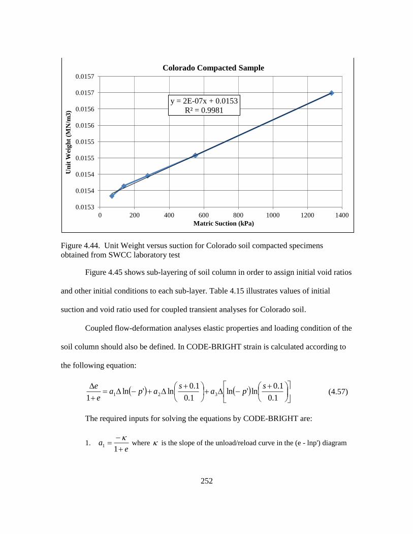
252
Figure 4.44. Unit Weight versus suction for Colorado soil compacted specimens
obtained from SWCC laboratory test
Figure 4.45 shows sub-layering of soil column in order to assign initial void ratios
and other initial conditions to each sub-layer. Table 4.15 illustrates values of initial
suction and void ratio used for coupled transient analyses for Colorado soil.
Coupled flow-deformation analyses elastic properties and loading condition of the
soil column should also be defined. In CODE-BRIGHT strain is calculated according to
the following equation:
1.0
1.0ln'ln
1.0
1.0ln'ln
1321
spa
sapa
e
e (4.57)
The required inputs for solving the equations by CODE-BRIGHT are:
1. e
a
11
where is the slope of the unload/reload curve in the (e - lnp') diagram
y = 2E-07x + 0.0153
R² = 0.9981
0.0153
0.0154
0.0154
0.0155
0.0155
0.0156
0.0156
0.0157
0.0157
0 200 400 600 800 1000 1200 1400
Un
it W
eig
ht
(MN
/m3
)
Matric Suction (kPa)
Colorado Compacted Sample
253
2. e
a s
12
where s is the slope of the unload/reload curve in the (e -
1.0
1.0ln
s)
diagram
3. 3a can be set as zero, which assumes that suction does not have a direct impact on
the mean stress
4. = Poisson’s ratio.
Values of a1 and a2 parameters were also determined for each sub-layer by having
initial void ratio and are listed in Table 4.15. Results of coupled analysis on Colorado soil
using CODE-BRIGHT including progression of change in water pressure and void ratio
versus elevation are shown in Figures 4.46 through 4.53. It can be seen from Figure 4.51
that although the initial void ratio profile is the same for both cases of corrected and
uncorrected SWCC's, the final void ratio of the case with uncorrected void ratio shows
larger values.
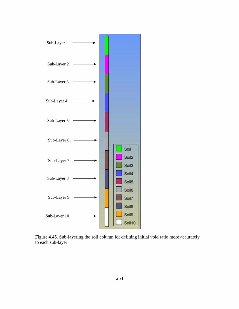
254
Figure 4.45. Sub-layering the soil column for defining initial void ratio more accurately
to each sub-layer
Sub-Layer 1
Sub-Layer 3
Sub-Layer 4
Sub-Layer 5
Sub-Layer 6
Sub-Layer 7
Sub-Layer 8
Sub-Layer 9
Sub-Layer 10
Sub-Layer 2
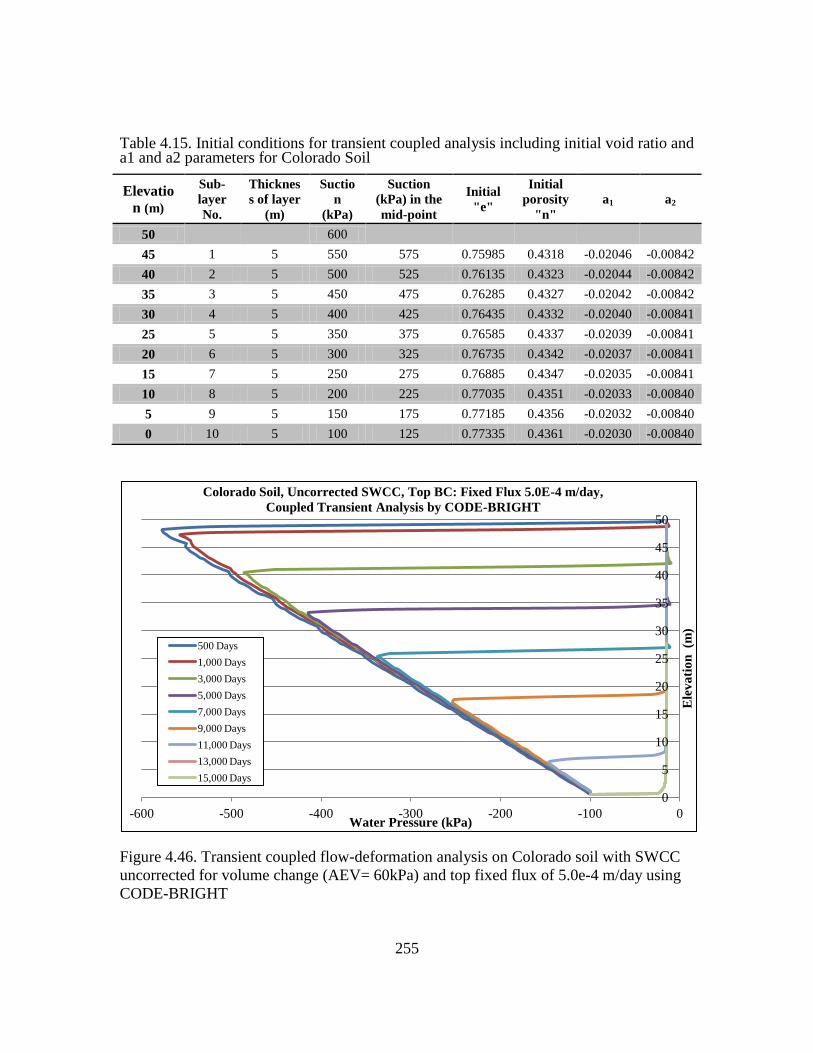
255
Table 4.15. Initial conditions for transient coupled analysis including initial void ratio and a1 and a2 parameters for Colorado Soil
Elevatio
n (m)
Sub-
layer
No.
Thicknes
s of layer
(m)
Suctio
n
(kPa)
Suction
(kPa) in the
mid-point
Initial
"e"
Initial
porosity
"n"
a1 a2
50
600
45 1 5 550 575 0.75985 0.4318 -0.02046 -0.00842
40 2 5 500 525 0.76135 0.4323 -0.02044 -0.00842
35 3 5 450 475 0.76285 0.4327 -0.02042 -0.00842
30 4 5 400 425 0.76435 0.4332 -0.02040 -0.00841
25 5 5 350 375 0.76585 0.4337 -0.02039 -0.00841
20 6 5 300 325 0.76735 0.4342 -0.02037 -0.00841
15 7 5 250 275 0.76885 0.4347 -0.02035 -0.00841
10 8 5 200 225 0.77035 0.4351 -0.02033 -0.00840
5 9 5 150 175 0.77185 0.4356 -0.02032 -0.00840
0 10 5 100 125 0.77335 0.4361 -0.02030 -0.00840
Figure 4.46. Transient coupled flow-deformation analysis on Colorado soil with SWCC
uncorrected for volume change (AEV= 60kPa) and top fixed flux of 5.0e-4 m/day using
CODE-BRIGHT
0
5
10
15
20
25
30
35
40
45
50
-600 -500 -400 -300 -200 -100 0
Ele
va
tio
n (m
)
Water Pressure (kPa)
Colorado Soil, Uncorrected SWCC, Top BC: Fixed Flux 5.0E-4 m/day,
Coupled Transient Analysis by CODE-BRIGHT
500 Days
1,000 Days
3,000 Days
5,000 Days
7,000 Days
9,000 Days
11,000 Days
13,000 Days
15,000 Days
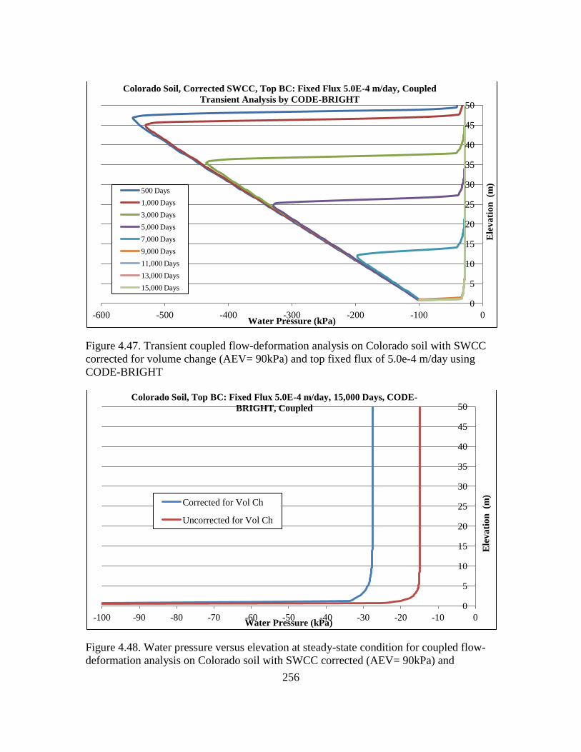
256
Figure 4.47. Transient coupled flow-deformation analysis on Colorado soil with SWCC
corrected for volume change (AEV= 90kPa) and top fixed flux of 5.0e-4 m/day using
CODE-BRIGHT
Figure 4.48. Water pressure versus elevation at steady-state condition for coupled flow-
deformation analysis on Colorado soil with SWCC corrected (AEV= 90kPa) and
0
5
10
15
20
25
30
35
40
45
50
-600 -500 -400 -300 -200 -100 0
Ele
va
tio
n (m
)
Water Pressure (kPa)
Colorado Soil, Corrected SWCC, Top BC: Fixed Flux 5.0E-4 m/day, Coupled
Transient Analysis by CODE-BRIGHT
500 Days
1,000 Days
3,000 Days
5,000 Days
7,000 Days
9,000 Days
11,000 Days
13,000 Days
15,000 Days
0
5
10
15
20
25
30
35
40
45
50
-100 -90 -80 -70 -60 -50 -40 -30 -20 -10 0
Ele
va
tio
n (m
)
Water Pressure (kPa)
Colorado Soil, Top BC: Fixed Flux 5.0E-4 m/day, 15,000 Days, CODE-
BRIGHT, Coupled
Corrected for Vol Ch
Uncorrected for Vol Ch
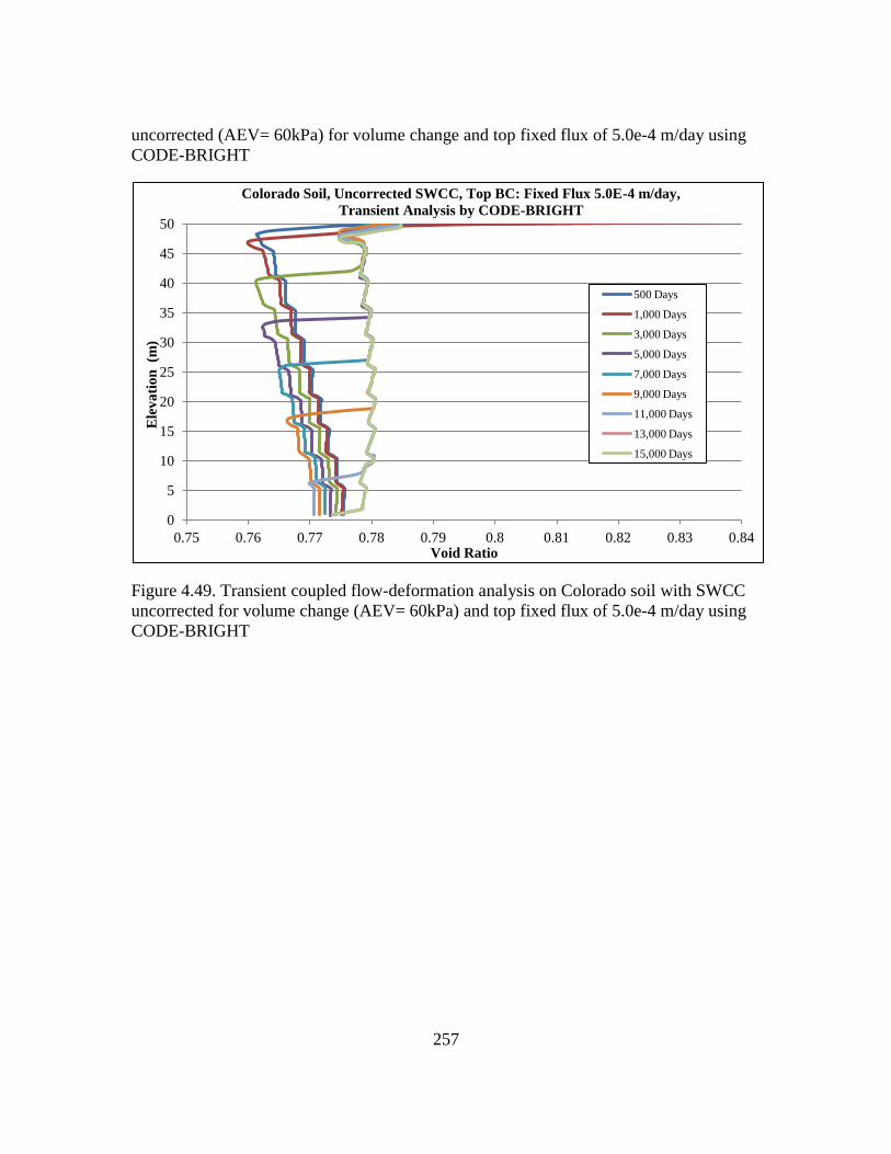
257
uncorrected (AEV= 60kPa) for volume change and top fixed flux of 5.0e-4 m/day using
CODE-BRIGHT
Figure 4.49. Transient coupled flow-deformation analysis on Colorado soil with SWCC
uncorrected for volume change (AEV= 60kPa) and top fixed flux of 5.0e-4 m/day using
CODE-BRIGHT
0
5
10
15
20
25
30
35
40
45
50
0.75 0.76 0.77 0.78 0.79 0.8 0.81 0.82 0.83 0.84
Ele
va
tio
n (m
)
Void Ratio
Colorado Soil, Uncorrected SWCC, Top BC: Fixed Flux 5.0E-4 m/day,
Transient Analysis by CODE-BRIGHT
500 Days
1,000 Days
3,000 Days
5,000 Days
7,000 Days
9,000 Days
11,000 Days
13,000 Days
15,000 Days
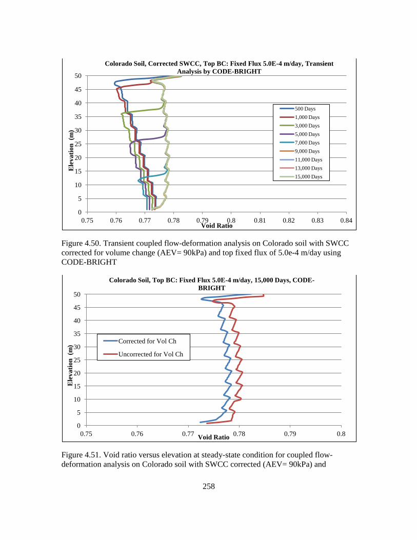
258
Figure 4.50. Transient coupled flow-deformation analysis on Colorado soil with SWCC
corrected for volume change (AEV= 90kPa) and top fixed flux of 5.0e-4 m/day using
CODE-BRIGHT
Figure 4.51. Void ratio versus elevation at steady-state condition for coupled flow-
deformation analysis on Colorado soil with SWCC corrected (AEV= 90kPa) and
0
5
10
15
20
25
30
35
40
45
50
0.75 0.76 0.77 0.78 0.79 0.8 0.81 0.82 0.83 0.84
Ele
va
tio
n (m
)
Void Ratio
Colorado Soil, Corrected SWCC, Top BC: Fixed Flux 5.0E-4 m/day, Transient
Analysis by CODE-BRIGHT
500 Days
1,000 Days
3,000 Days
5,000 Days
7,000 Days
9,000 Days
11,000 Days
13,000 Days
15,000 Days
0
5
10
15
20
25
30
35
40
45
50
0.75 0.76 0.77 0.78 0.79 0.8
Ele
va
tio
n (m
)
Void Ratio
Colorado Soil, Top BC: Fixed Flux 5.0E-4 m/day, 15,000 Days, CODE-
BRIGHT
Corrected for Vol Ch
Uncorrected for Vol Ch
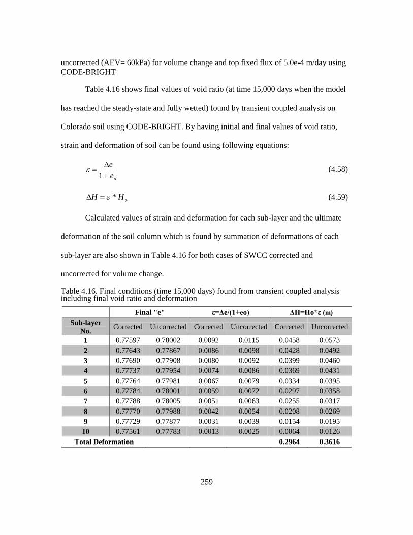
259
uncorrected (AEV= 60kPa) for volume change and top fixed flux of 5.0e-4 m/day using
CODE-BRIGHT
Table 4.16 shows final values of void ratio (at time 15,000 days when the model
has reached the steady-state and fully wetted) found by transient coupled analysis on
Colorado soil using CODE-BRIGHT. By having initial and final values of void ratio,
strain and deformation of soil can be found using following equations:
oe
e
1 (4.58)
oHH * (4.59)
Calculated values of strain and deformation for each sub-layer and the ultimate
deformation of the soil column which is found by summation of deformations of each
sub-layer are also shown in Table 4.16 for both cases of SWCC corrected and
uncorrected for volume change.
Table 4.16. Final conditions (time 15,000 days) found from transient coupled analysis including final void ratio and deformation
Final "e" ε=Δe/(1+eo) ΔH=Ho*ε (m)
Sub-layer
No. Corrected Uncorrected Corrected Uncorrected Corrected Uncorrected
1 0.77597 0.78002 0.0092 0.0115 0.0458 0.0573
2 0.77643 0.77867 0.0086 0.0098 0.0428 0.0492
3 0.77690 0.77908 0.0080 0.0092 0.0399 0.0460
4 0.77737 0.77954 0.0074 0.0086 0.0369 0.0431
5 0.77764 0.77981 0.0067 0.0079 0.0334 0.0395
6 0.77784 0.78001 0.0059 0.0072 0.0297 0.0358
7 0.77788 0.78005 0.0051 0.0063 0.0255 0.0317
8 0.77770 0.77988 0.0042 0.0054 0.0208 0.0269
9 0.77729 0.77877 0.0031 0.0039 0.0154 0.0195
10 0.77561 0.77783 0.0013 0.0025 0.0064 0.0126
Total Deformation
0.2964 0.3616
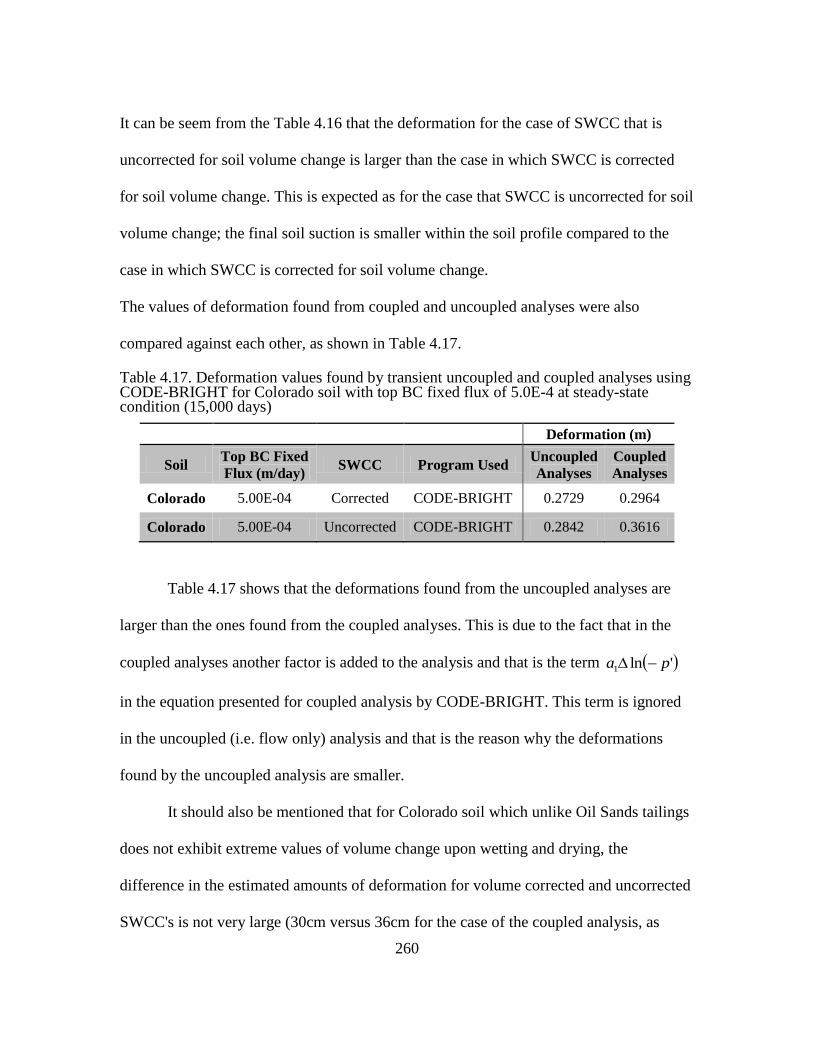
260
It can be seem from the Table 4.16 that the deformation for the case of SWCC that is
uncorrected for soil volume change is larger than the case in which SWCC is corrected
for soil volume change. This is expected as for the case that SWCC is uncorrected for soil
volume change; the final soil suction is smaller within the soil profile compared to the
case in which SWCC is corrected for soil volume change.
The values of deformation found from coupled and uncoupled analyses were also
compared against each other, as shown in Table 4.17.
Table 4.17. Deformation values found by transient uncoupled and coupled analyses using CODE-BRIGHT for Colorado soil with top BC fixed flux of 5.0E-4 at steady-state condition (15,000 days)
Deformation (m)
Soil Top BC Fixed
Flux (m/day) SWCC Program Used
Uncoupled
Analyses
Coupled
Analyses
Colorado 5.00E-04 Corrected CODE-BRIGHT 0.2729 0.2964
Colorado 5.00E-04 Uncorrected CODE-BRIGHT 0.2842 0.3616
Table 4.17 shows that the deformations found from the uncoupled analyses are
larger than the ones found from the coupled analyses. This is due to the fact that in the
coupled analyses another factor is added to the analysis and that is the term 'ln1 pa
in the equation presented for coupled analysis by CODE-BRIGHT. This term is ignored
in the uncoupled (i.e. flow only) analysis and that is the reason why the deformations
found by the uncoupled analysis are smaller.
It should also be mentioned that for Colorado soil which unlike Oil Sands tailings
does not exhibit extreme values of volume change upon wetting and drying, the
difference in the estimated amounts of deformation for volume corrected and uncorrected
SWCC's is not very large (30cm versus 36cm for the case of the coupled analysis, as
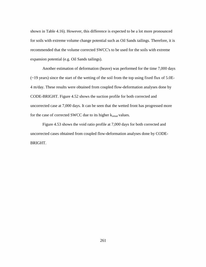
261
shown in Table 4.16). However, this difference is expected to be a lot more pronounced
for soils with extreme volume change potential such as Oil Sands tailings. Therefore, it is
recommended that the volume corrected SWCC's to be used for the soils with extreme
expansion potential (e.g. Oil Sands tailings).
Another estimation of deformation (heave) was performed for the time 7,000 days
(~19 years) since the start of the wetting of the soil from the top using fixed flux of 5.0E-
4 m/day. These results were obtained from coupled flow-deformation analyses done by
CODE-BRIGHT. Figure 4.52 shows the suction profile for both corrected and
uncorrected case at 7,000 days. It can be seen that the wetted front has progressed more
for the case of corrected SWCC due to its higher kunsat values.
Figure 4.53 shows the void ratio profile at 7,000 days for both corrected and
uncorrected cases obtained from coupled flow-deformation analyses done by CODE-
BRIGHT.
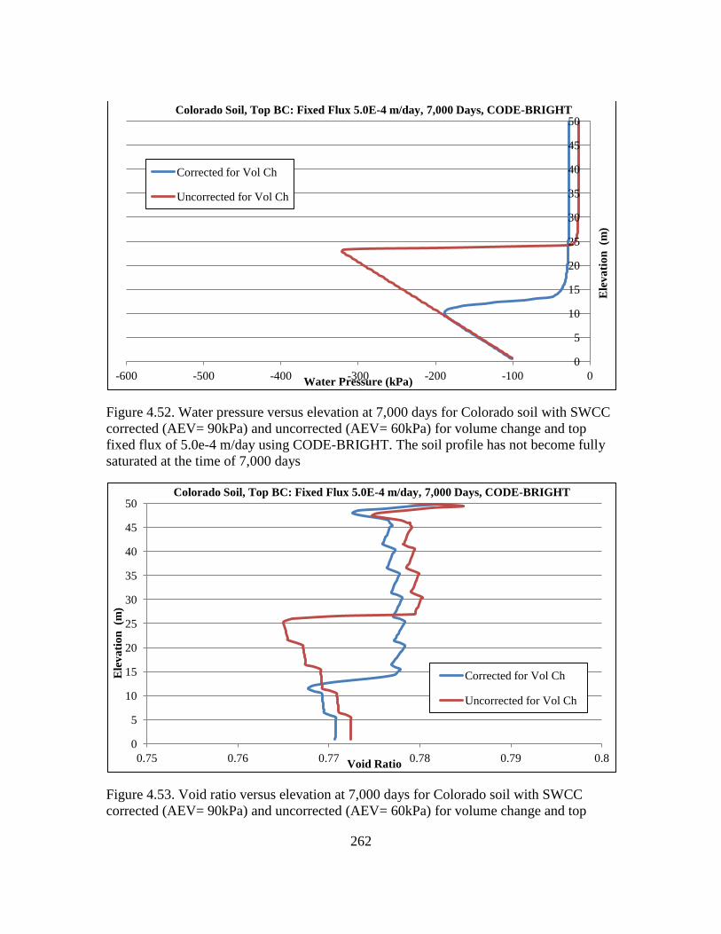
262
Figure 4.52. Water pressure versus elevation at 7,000 days for Colorado soil with SWCC
corrected (AEV= 90kPa) and uncorrected (AEV= 60kPa) for volume change and top
fixed flux of 5.0e-4 m/day using CODE-BRIGHT. The soil profile has not become fully
saturated at the time of 7,000 days
Figure 4.53. Void ratio versus elevation at 7,000 days for Colorado soil with SWCC
corrected (AEV= 90kPa) and uncorrected (AEV= 60kPa) for volume change and top
0
5
10
15
20
25
30
35
40
45
50
-600 -500 -400 -300 -200 -100 0
Ele
va
tio
n (m
)
Water Pressure (kPa)
Colorado Soil, Top BC: Fixed Flux 5.0E-4 m/day, 7,000 Days, CODE-BRIGHT
Corrected for Vol Ch
Uncorrected for Vol Ch
0
5
10
15
20
25
30
35
40
45
50
0.75 0.76 0.77 0.78 0.79 0.8
Ele
va
tio
n (m
)
Void Ratio
Colorado Soil, Top BC: Fixed Flux 5.0E-4 m/day, 7,000 Days, CODE-BRIGHT
Corrected for Vol Ch
Uncorrected for Vol Ch
263
fixed flux of 5.0e-4 m/day using CODE-BRIGHT. The soil profile has not become fully
saturated at the time of 7,000 days
Table 4.18 shows the void ratio profile at 7,000 days for both corrected and
uncorrected cases obtained from the couple flow-deformation analyses by CODE-
BRIGHT. This table also shows the amounts of deformation (heave) for uncorrected and
corrected SWCC at time 7,000 days. It can be seen that the corrected SWCC shows more
deformation. It should be mentioned that for the case of long-term wetting of the soil
(where the whole soil profile becomes saturated) the deformation of the uncorrected case
is larger than the deformation of the corrected case. Therefore, it is difficult to determine
in advance if corrected or uncorrected curves will lead to higher suction values and
deformation within the profile.
Table 4.19 compares amounts of heave found from transient coupled and
uncoupled analyses at time 7,000 days performed by CODE-BRIGHT. It can be seen that
there is a very good agreement between the results found from coupled and uncoupled
analyses for both corrected and uncorrected SWCC's.
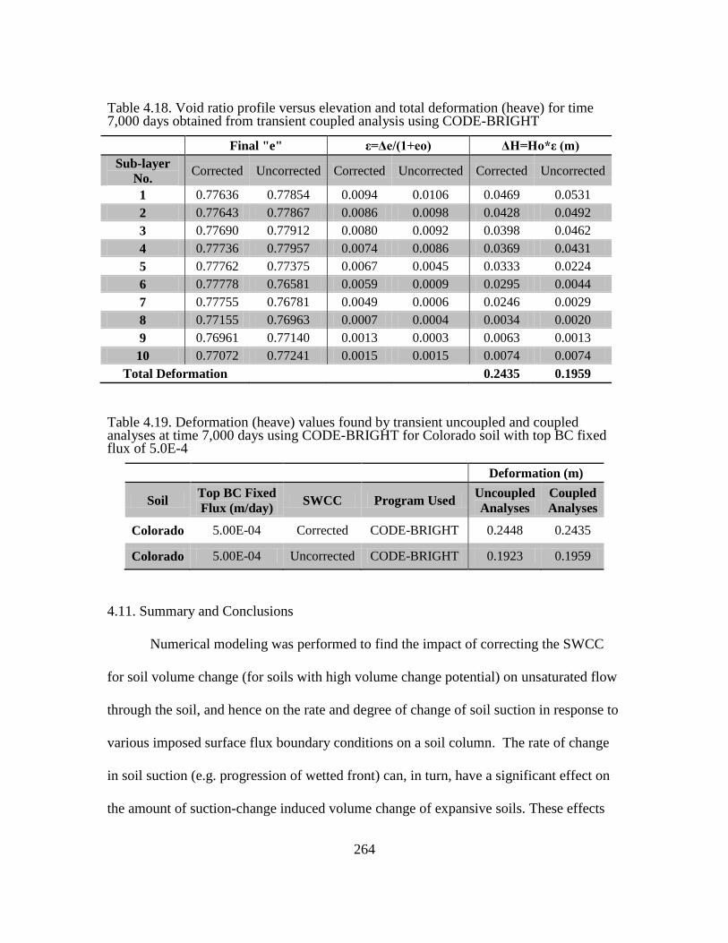
264
Table 4.18. Void ratio profile versus elevation and total deformation (heave) for time 7,000 days obtained from transient coupled analysis using CODE-BRIGHT
Final "e" ε=Δe/(1+eo) ΔH=Ho*ε (m)
Sub-layer
No. Corrected Uncorrected Corrected Uncorrected Corrected Uncorrected
1 0.77636 0.77854 0.0094 0.0106 0.0469 0.0531
2 0.77643 0.77867 0.0086 0.0098 0.0428 0.0492
3 0.77690 0.77912 0.0080 0.0092 0.0398 0.0462
4 0.77736 0.77957 0.0074 0.0086 0.0369 0.0431
5 0.77762 0.77375 0.0067 0.0045 0.0333 0.0224
6 0.77778 0.76581 0.0059 0.0009 0.0295 0.0044
7 0.77755 0.76781 0.0049 0.0006 0.0246 0.0029
8 0.77155 0.76963 0.0007 0.0004 0.0034 0.0020
9 0.76961 0.77140 0.0013 0.0003 0.0063 0.0013
10 0.77072 0.77241 0.0015 0.0015 0.0074 0.0074
Total Deformation
0.2435 0.1959
Table 4.19. Deformation (heave) values found by transient uncoupled and coupled analyses at time 7,000 days using CODE-BRIGHT for Colorado soil with top BC fixed flux of 5.0E-4
Deformation (m)
Soil Top BC Fixed
Flux (m/day) SWCC Program Used
Uncoupled
Analyses
Coupled
Analyses
Colorado 5.00E-04 Corrected CODE-BRIGHT 0.2448 0.2435
Colorado 5.00E-04 Uncorrected CODE-BRIGHT 0.1923 0.1959
4.11. Summary and Conclusions
Numerical modeling was performed to find the impact of correcting the SWCC
for soil volume change (for soils with high volume change potential) on unsaturated flow
through the soil, and hence on the rate and degree of change of soil suction in response to
various imposed surface flux boundary conditions on a soil column. The rate of change
in soil suction (e.g. progression of wetted front) can, in turn, have a significant effect on
the amount of suction-change induced volume change of expansive soils. These effects
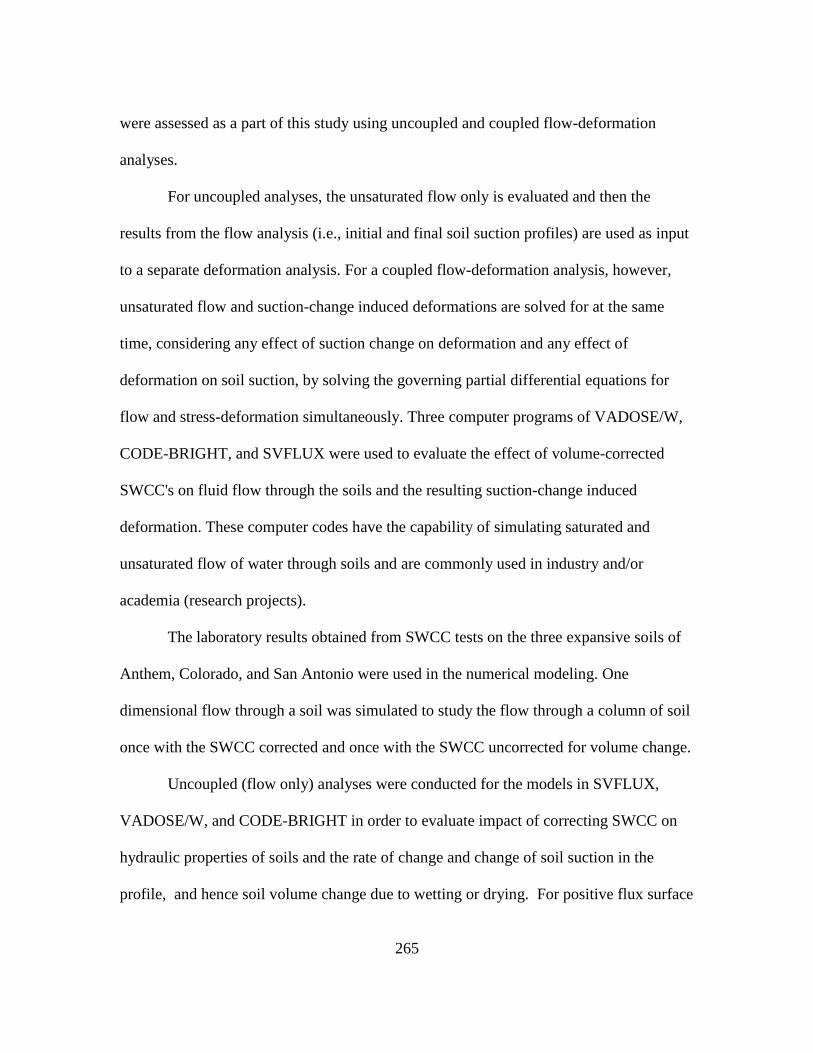
265
were assessed as a part of this study using uncoupled and coupled flow-deformation
analyses.
For uncoupled analyses, the unsaturated flow only is evaluated and then the
results from the flow analysis (i.e., initial and final soil suction profiles) are used as input
to a separate deformation analysis. For a coupled flow-deformation analysis, however,
unsaturated flow and suction-change induced deformations are solved for at the same
time, considering any effect of suction change on deformation and any effect of
deformation on soil suction, by solving the governing partial differential equations for
flow and stress-deformation simultaneously. Three computer programs of VADOSE/W,
CODE-BRIGHT, and SVFLUX were used to evaluate the effect of volume-corrected
SWCC's on fluid flow through the soils and the resulting suction-change induced
deformation. These computer codes have the capability of simulating saturated and
unsaturated flow of water through soils and are commonly used in industry and/or
academia (research projects).
The laboratory results obtained from SWCC tests on the three expansive soils of
Anthem, Colorado, and San Antonio were used in the numerical modeling. One
dimensional flow through a soil was simulated to study the flow through a column of soil
once with the SWCC corrected and once with the SWCC uncorrected for volume change.
Uncoupled (flow only) analyses were conducted for the models in SVFLUX,
VADOSE/W, and CODE-BRIGHT in order to evaluate impact of correcting SWCC on
hydraulic properties of soils and the rate of change and change of soil suction in the
profile, and hence soil volume change due to wetting or drying. For positive flux surface
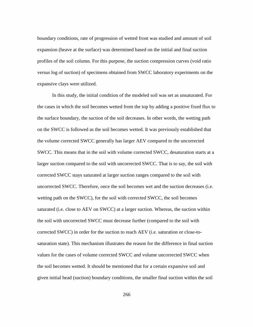
266
boundary conditions, rate of progression of wetted front was studied and amount of soil
expansion (heave at the surface) was determined based on the initial and final suction
profiles of the soil column. For this purpose, the suction compression curves (void ratio
versus log of suction) of specimens obtained from SWCC laboratory experiments on the
expansive clays were utilized.
In this study, the initial condition of the modeled soil was set as unsaturated. For
the cases in which the soil becomes wetted from the top by adding a positive fixed flux to
the surface boundary, the suction of the soil decreases. In other words, the wetting path
on the SWCC is followed as the soil becomes wetted. It was previously established that
the volume corrected SWCC generally has larger AEV compared to the uncorrected
SWCC. This means that in the soil with volume corrected SWCC, desaturation starts at a
larger suction compared to the soil with uncorrected SWCC. That is to say, the soil with
corrected SWCC stays saturated at larger suction ranges compared to the soil with
uncorrected SWCC. Therefore, once the soil becomes wet and the suction decreases (i.e.
wetting path on the SWCC), for the soil with corrected SWCC, the soil becomes
saturated (i.e. close to AEV on SWCC) at a larger suction. Whereas, the suction within
the soil with uncorrected SWCC must decrease further (compared to the soil with
corrected SWCC) in order for the suction to reach AEV (i.e. saturation or close-to-
saturation state). This mechanism illustrates the reason for the difference in final suction
values for the cases of volume corrected SWCC and volume uncorrected SWCC when
the soil becomes wetted. It should be mentioned that for a certain expansive soil and
given initial head (suction) boundary conditions, the smaller final suction within the soil
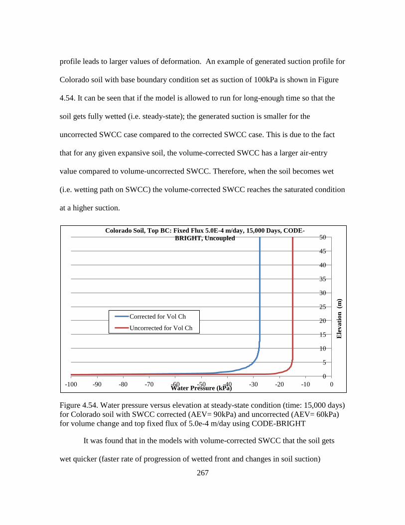
267
profile leads to larger values of deformation. An example of generated suction profile for
Colorado soil with base boundary condition set as suction of 100kPa is shown in Figure
4.54. It can be seen that if the model is allowed to run for long-enough time so that the
soil gets fully wetted (i.e. steady-state); the generated suction is smaller for the
uncorrected SWCC case compared to the corrected SWCC case. This is due to the fact
that for any given expansive soil, the volume-corrected SWCC has a larger air-entry
value compared to volume-uncorrected SWCC. Therefore, when the soil becomes wet
(i.e. wetting path on SWCC) the volume-corrected SWCC reaches the saturated condition
at a higher suction.
Figure 4.54. Water pressure versus elevation at steady-state condition (time: 15,000 days)
for Colorado soil with SWCC corrected (AEV= 90kPa) and uncorrected (AEV= 60kPa)
for volume change and top fixed flux of 5.0e-4 m/day using CODE-BRIGHT
It was found that in the models with volume-corrected SWCC that the soil gets
wet quicker (faster rate of progression of wetted front and changes in soil suction)
0
5
10
15
20
25
30
35
40
45
50
-100 -90 -80 -70 -60 -50 -40 -30 -20 -10 0
Ele
va
tio
n (m
)
Water Pressure (kPa)
Colorado Soil, Top BC: Fixed Flux 5.0E-4 m/day, 15,000 Days, CODE-
BRIGHT, Uncoupled
Corrected for Vol Ch
Uncorrected for Vol Ch

268
because the unsaturated hydraulic conductivity of the soil with corrected SWCC is higher
than the unsaturated hydraulic conductivity of the same soil with volume uncorrected
SWCC. Larger values of kunsat result in faster water penetration through the soil.
For the times prior to the steady-state, in some portions of the soil profile, the
suction of uncorrected SWCC is higher than the suction of the corrected SWCC. This is
due to the fact that kunsat is generally higher for corrected SWCC and hence, at a given
time, the depth of wetting is generally larger for the corrected SWCC compared to
uncorrected SWCC. This may lead to overall larger heave for the corrected SWCC
compared to uncorrected SWCC at certain times during the analysis. Figure 4.55 shows
an example which compares the depth of wetting of volume-corrected and volume-
uncorrected SWCC at the time of 7,000 days for top boundary condition of fixed flux of
5.0E-4 m/day for Colorado soil. It can be seen that the depth of wetting is larger for
corrected SWCC (due to higher kunsat values).
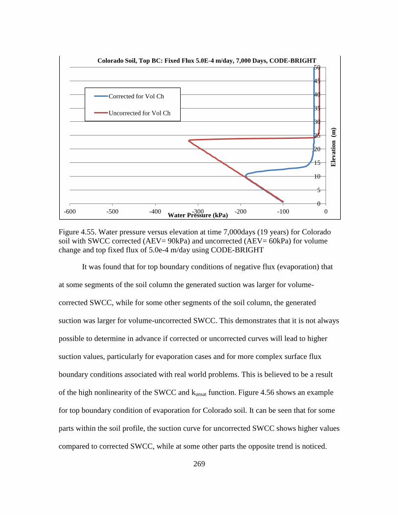
269
Figure 4.55. Water pressure versus elevation at time 7,000days (19 years) for Colorado
soil with SWCC corrected (AEV= 90kPa) and uncorrected (AEV= 60kPa) for volume
change and top fixed flux of 5.0e-4 m/day using CODE-BRIGHT
It was found that for top boundary conditions of negative flux (evaporation) that
at some segments of the soil column the generated suction was larger for volume-
corrected SWCC, while for some other segments of the soil column, the generated
suction was larger for volume-uncorrected SWCC. This demonstrates that it is not always
possible to determine in advance if corrected or uncorrected curves will lead to higher
suction values, particularly for evaporation cases and for more complex surface flux
boundary conditions associated with real world problems. This is believed to be a result
of the high nonlinearity of the SWCC and kunsat function. Figure 4.56 shows an example
for top boundary condition of evaporation for Colorado soil. It can be seen that for some
parts within the soil profile, the suction curve for uncorrected SWCC shows higher values
compared to corrected SWCC, while at some other parts the opposite trend is noticed.
0
5
10
15
20
25
30
35
40
45
50
-600 -500 -400 -300 -200 -100 0
Ele
va
tio
n (m
)
Water Pressure (kPa)
Colorado Soil, Top BC: Fixed Flux 5.0E-4 m/day, 7,000 Days, CODE-BRIGHT
Corrected for Vol Ch
Uncorrected for Vol Ch
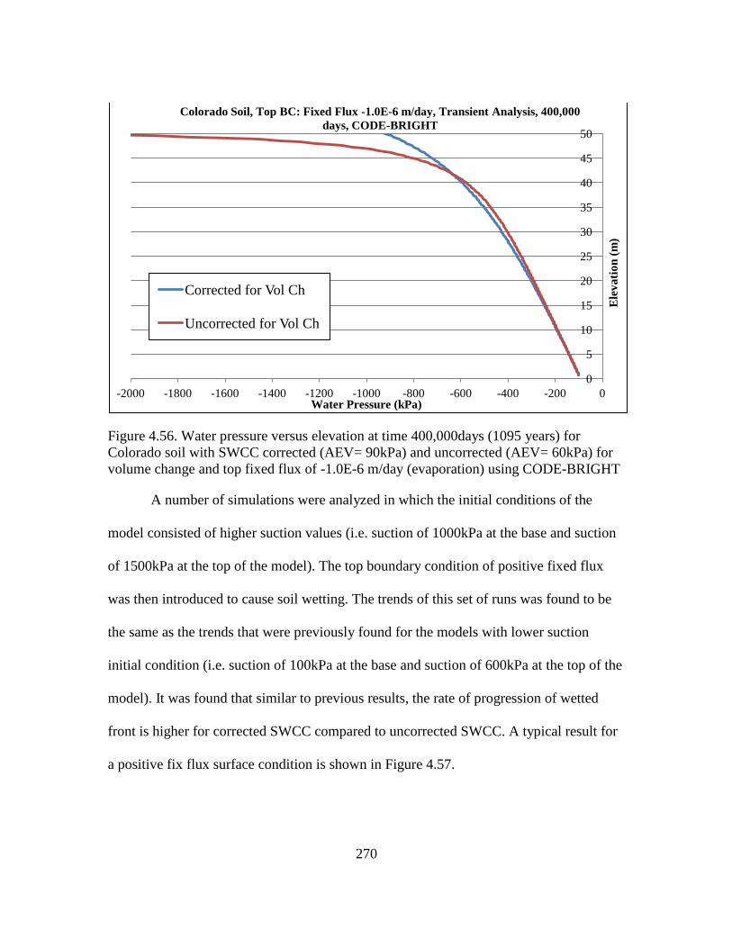
270
Figure 4.56. Water pressure versus elevation at time 400,000days (1095 years) for
Colorado soil with SWCC corrected (AEV= 90kPa) and uncorrected (AEV= 60kPa) for
volume change and top fixed flux of -1.0E-6 m/day (evaporation) using CODE-BRIGHT
A number of simulations were analyzed in which the initial conditions of the
model consisted of higher suction values (i.e. suction of 1000kPa at the base and suction
of 1500kPa at the top of the model). The top boundary condition of positive fixed flux
was then introduced to cause soil wetting. The trends of this set of runs was found to be
the same as the trends that were previously found for the models with lower suction
initial condition (i.e. suction of 100kPa at the base and suction of 600kPa at the top of the
model). It was found that similar to previous results, the rate of progression of wetted
front is higher for corrected SWCC compared to uncorrected SWCC. A typical result for
a positive fix flux surface condition is shown in Figure 4.57.
0
5
10
15
20
25
30
35
40
45
50
-2000 -1800 -1600 -1400 -1200 -1000 -800 -600 -400 -200 0
Ele
va
tio
n (
m)
Water Pressure (kPa)
Colorado Soil, Top BC: Fixed Flux -1.0E-6 m/day, Transient Analysis, 400,000
days, CODE-BRIGHT
Corrected for Vol Ch
Uncorrected for Vol Ch
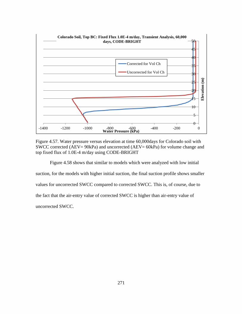
271
Figure 4.57. Water pressure versus elevation at time 60,000days for Colorado soil with
SWCC corrected (AEV= 90kPa) and uncorrected (AEV= 60kPa) for volume change and
top fixed flux of 1.0E-4 m/day using CODE-BRIGHT
Figure 4.58 shows that similar to models which were analyzed with low initial
suction, for the models with higher initial suction, the final suction profile shows smaller
values for uncorrected SWCC compared to corrected SWCC. This is, of course, due to
the fact that the air-entry value of corrected SWCC is higher than air-entry value of
uncorrected SWCC.
0
5
10
15
20
25
30
35
40
45
50
-1400 -1200 -1000 -800 -600 -400 -200 0
Ele
va
tio
n (
m)
Water Pressure (kPa)
Colorado Soil, Top BC: Fixed Flux 1.0E-4 m/day, Transient Analysis, 60,000
days, CODE-BRIGHT
Corrected for Vol Ch
Uncorrected for Vol Ch
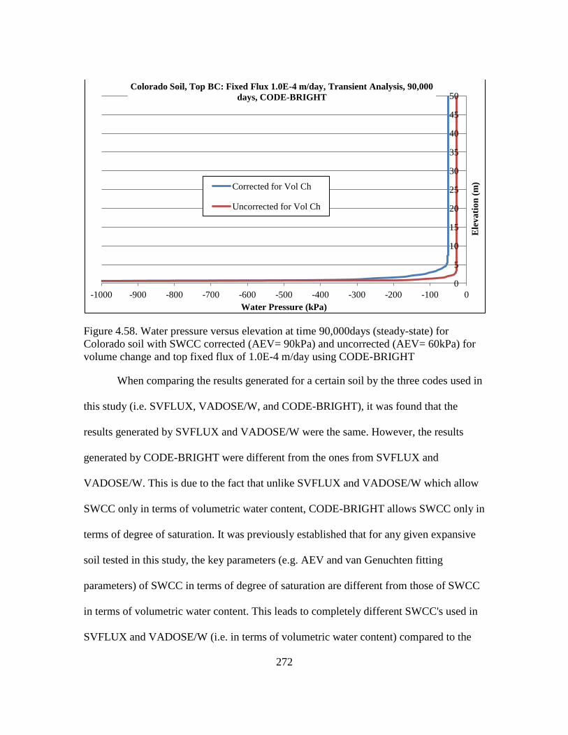
272
Figure 4.58. Water pressure versus elevation at time 90,000days (steady-state) for
Colorado soil with SWCC corrected (AEV= 90kPa) and uncorrected (AEV= 60kPa) for
volume change and top fixed flux of 1.0E-4 m/day using CODE-BRIGHT
When comparing the results generated for a certain soil by the three codes used in
this study (i.e. SVFLUX, VADOSE/W, and CODE-BRIGHT), it was found that the
results generated by SVFLUX and VADOSE/W were the same. However, the results
generated by CODE-BRIGHT were different from the ones from SVFLUX and
VADOSE/W. This is due to the fact that unlike SVFLUX and VADOSE/W which allow
SWCC only in terms of volumetric water content, CODE-BRIGHT allows SWCC only in
terms of degree of saturation. It was previously established that for any given expansive
soil tested in this study, the key parameters (e.g. AEV and van Genuchten fitting
parameters) of SWCC in terms of degree of saturation are different from those of SWCC
in terms of volumetric water content. This leads to completely different SWCC's used in
SVFLUX and VADOSE/W (i.e. in terms of volumetric water content) compared to the
0
5
10
15
20
25
30
35
40
45
50
-1000 -900 -800 -700 -600 -500 -400 -300 -200 -100 0
Ele
va
tio
n (
m)
Water Pressure (kPa)
Colorado Soil, Top BC: Fixed Flux 1.0E-4 m/day, Transient Analysis, 90,000
days, CODE-BRIGHT
Corrected for Vol Ch
Uncorrected for Vol Ch
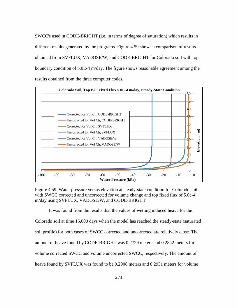
273
SWCC's used in CODE-BRIGHT (i.e. in terms of degree of saturation) which results in
different results generated by the programs. Figure 4.59 shows a comparison of results
obtained from SVFLUX, VADOSE/W, and CODE-BRIGHT for Colorado soil with top
boundary condition of 5.0E-4 m/day. The figure shows reasonable agreement among the
results obtained from the three computer codes.
Figure 4.59. Water pressure versus elevation at steady-state condition for Colorado soil
with SWCC corrected and uncorrected for volume change and top fixed flux of 5.0e-4
m/day using SVFLUX, VADOSE/W, and CODE-BRIGHT
It was found from the results that the values of wetting induced heave for the
Colorado soil at time 15,000 days when the model has reached the steady-state (saturated
soil profile) for both cases of SWCC corrected and uncorrected are relatively close. The
amount of heave found by CODE-BRIGHT was 0.2729 meters and 0.2842 meters for
volume corrected SWCC and volume uncorrected SWCC, respectively. The amount of
heave found by SVFLUX was found to be 0.2908 meters and 0.2931 meters for volume
0
5
10
15
20
25
30
35
40
45
50
-100 -90 -80 -70 -60 -50 -40 -30 -20 -10 0
Ele
va
tio
n (m
)
Water Pressure (kPa)
Colorado Soil, Top BC: Fixed Flux 5.0E-4 m/day, Steady-State Condition
Corrected for Vol Ch, CODE-BRIGHT
Uncorrected for Vol Ch, CODE-BRIGHT
Corrected for Vol Ch, SVFLUX
Uncorrected for Vol Ch, SVFLUX
Corrected for Vol Ch, VADOSE/W
Uncorrected for Vol Ch, VADOSE/W
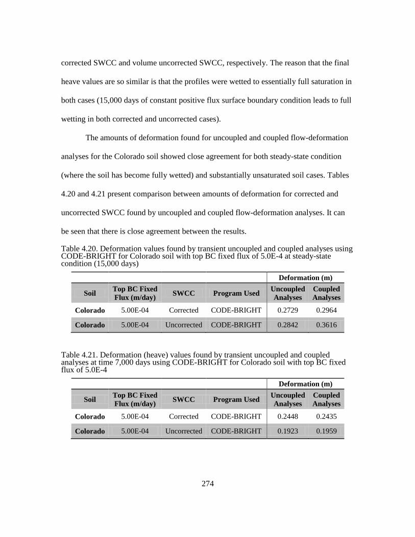
274
corrected SWCC and volume uncorrected SWCC, respectively. The reason that the final
heave values are so similar is that the profiles were wetted to essentially full saturation in
both cases (15,000 days of constant positive flux surface boundary condition leads to full
wetting in both corrected and uncorrected cases).
The amounts of deformation found for uncoupled and coupled flow-deformation
analyses for the Colorado soil showed close agreement for both steady-state condition
(where the soil has become fully wetted) and substantially unsaturated soil cases. Tables
4.20 and 4.21 present comparison between amounts of deformation for corrected and
uncorrected SWCC found by uncoupled and coupled flow-deformation analyses. It can
be seen that there is close agreement between the results.
Table 4.20. Deformation values found by transient uncoupled and coupled analyses using CODE-BRIGHT for Colorado soil with top BC fixed flux of 5.0E-4 at steady-state condition (15,000 days)
Deformation (m)
Soil Top BC Fixed
Flux (m/day) SWCC Program Used
Uncoupled
Analyses
Coupled
Analyses
Colorado 5.00E-04 Corrected CODE-BRIGHT 0.2729 0.2964
Colorado 5.00E-04 Uncorrected CODE-BRIGHT 0.2842 0.3616
Table 4.21. Deformation (heave) values found by transient uncoupled and coupled analyses at time 7,000 days using CODE-BRIGHT for Colorado soil with top BC fixed flux of 5.0E-4
Deformation (m)
Soil Top BC Fixed
Flux (m/day) SWCC Program Used
Uncoupled
Analyses
Coupled
Analyses
Colorado 5.00E-04 Corrected CODE-BRIGHT 0.2448 0.2435
Colorado 5.00E-04 Uncorrected CODE-BRIGHT 0.1923 0.1959
275
It was found from the uncoupled and coupled flow-deformation analyses on
Colorado soil with top boundary condition of fixed flux of 5.0e-4 m/day that at time
7,000 days when the models has not reached the steady-state (not fully wetted), the
deformation is larger for corrected SWCC compared to uncorrected SWCC (0.245m and
0.19m for corrected and uncorrected cases, respectively). This is due to higher rate of
progression of wetted front for the case of corrected SWCC compared to uncorrected
SWCC. The difference in deformation of volume-corrected and volume-uncorrected
cases were found to be smaller at steady-state (full saturation) condition, compared to the
earlier times in the process (i.e. when the soils have not become saturated), as expected. It
was also found that for the conditions of fully wetted soils, the deformation is slightly
larger for volume-uncorrected SWCC (due to smaller suction values within the profile)
compared to volume-corrected SWCC. However, at times prior to steady-state (when the
soil is not saturated) the deformation was found to be larger for volume-corrected SWCC
because the water progresses more rapidly through the volume-corrected soil profile case.
It should also be mentioned that for the expansive soils in this study, which do not
exhibit extreme volume change upon wetting and drying, the difference in the estimated
amounts of deformation for volume corrected and uncorrected SWCC's is not very large.
However, this difference is expected to be significantly more pronounced for more highly
expansive soils (e.g. higher PI soils), for conditions resulting in larger changes in soil
suction, and also for any extremely high volume change soils, such as slurry materials.
The effect of volume change on the shape of the SWCC, including AEV and
slope in the transition zone, is clearly demonstrated, and when volume change corrections

276
are not made, it results in an error in the AEV and slope of the SWCC. However, it is
less clear whether volume change corrections to the SWCC in estimating kunsat functions
leads to improved unsaturated flow results. The uncertainty results from the fact that the
kunsat function models have been developed using data that was not volume corrected.
This may lead to existence of compensating errors in the analyses. On the other hand,
most of the data used for developing and validating kunsat function models was not on
clays, but rather on silts and sands and materials with no significant volume change.
Therefore, correcting the SWCC's for volume change may be a reasonable practice for
soils with high volume change potential (such as expansive soils and slurry specimens).
More studies are definitely needed in this area to evaluate the effect of change on SWCC
key parameters, particularly AEV and slope in transition zone, on the unsaturated flow
properties (kunsat versus suction) of high volume change soils. The study here on effects of
volume change on SWCC's, kunsat functions, and unsaturated flow/deformation analyses
represents only a start on understanding the complex issues at play for unsaturated
flow/deformation modeling of high volume change soils.
277
Chapter 5
NUMERICAL MODELING OF OIL SANDS TAILINGS
5.1. Introduction
Computer codes VADOSE/W, SVFLUX, and CODE-BRIGHT were used to
model one-dimensional flow through a soil column of oil sands tailings. The geometry
and initial and boundary conditions for oil sands tailings modeling were the same as the
models for expansive soils analyses described in Chapter 4.
The properties of Oil Sands tailings were obtained from the studies that were
previously conducted by Fredlund and Houston (2013), and Fredlund et al. (2011).
Fredlund et al. (2011) presented some of the properties of oil sands tailings. The authors
measured and established SWCC's of Oil Sands tailings that were mixed with 10% sand
and 45% sand. The material with 10% sand was found to have plastic and liquid limits of
30 and 55, respectively (PI= 25). The material with 45% sand was found to have plastic
and liquid limits of 15 and 38 (PI= 23) (Fredlund et al., 2011). The authors mentioned
that approximately 60% of the material classifies as clay size particles.
The SWCC's of oil sands tailings were established by drying SWCC testing of the
slurry specimens. The initially saturated slurry specimens of oil sands tailings exhibit
extreme volume change upon increase in suction. Slurry specimens of oil sands tailings
exhibit shrinkage as suction is increased, including at suction values smaller than air-
entry value when the specimen is still saturated. Volume changes that occur at suctions
smaller than the air-entry value can be quite significant for the oil sands, and therefore
affect the ksat value of these specimens. It is recommended that the value of ksat be
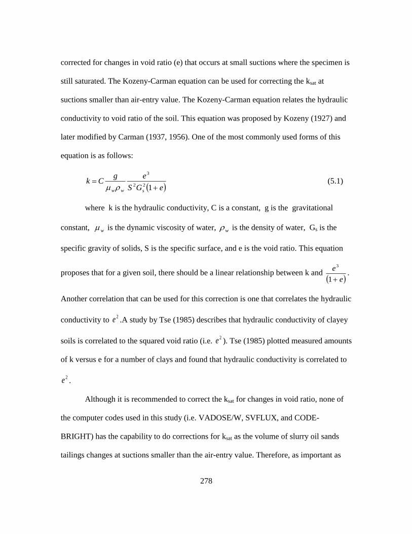
278
corrected for changes in void ratio (e) that occurs at small suctions where the specimen is
still saturated. The Kozeny-Carman equation can be used for correcting the ksat at
suctions smaller than air-entry value. The Kozeny-Carman equation relates the hydraulic
conductivity to void ratio of the soil. This equation was proposed by Kozeny (1927) and
later modified by Carman (1937, 1956). One of the most commonly used forms of this
equation is as follows:
eGS
egCk
sww
122
3
(5.1)
where k is the hydraulic conductivity, C is a constant, g is the gravitational
constant, w is the dynamic viscosity of water, w is the density of water, Gs is the
specific gravity of solids, S is the specific surface, and e is the void ratio. This equation
proposes that for a given soil, there should be a linear relationship between k and e
e
1
3
.
Another correlation that can be used for this correction is one that correlates the hydraulic
conductivity to 2e .A study by Tse (1985) describes that hydraulic conductivity of clayey
soils is correlated to the squared void ratio (i.e. 2e ). Tse (1985) plotted measured amounts
of k versus e for a number of clays and found that hydraulic conductivity is correlated to
2e .
Although it is recommended to correct the ksat for changes in void ratio, none of
the computer codes used in this study (i.e. VADOSE/W, SVFLUX, and CODE-
BRIGHT) has the capability to do corrections for ksat as the volume of slurry oil sands
tailings changes at suctions smaller than the air-entry value. Therefore, as important as
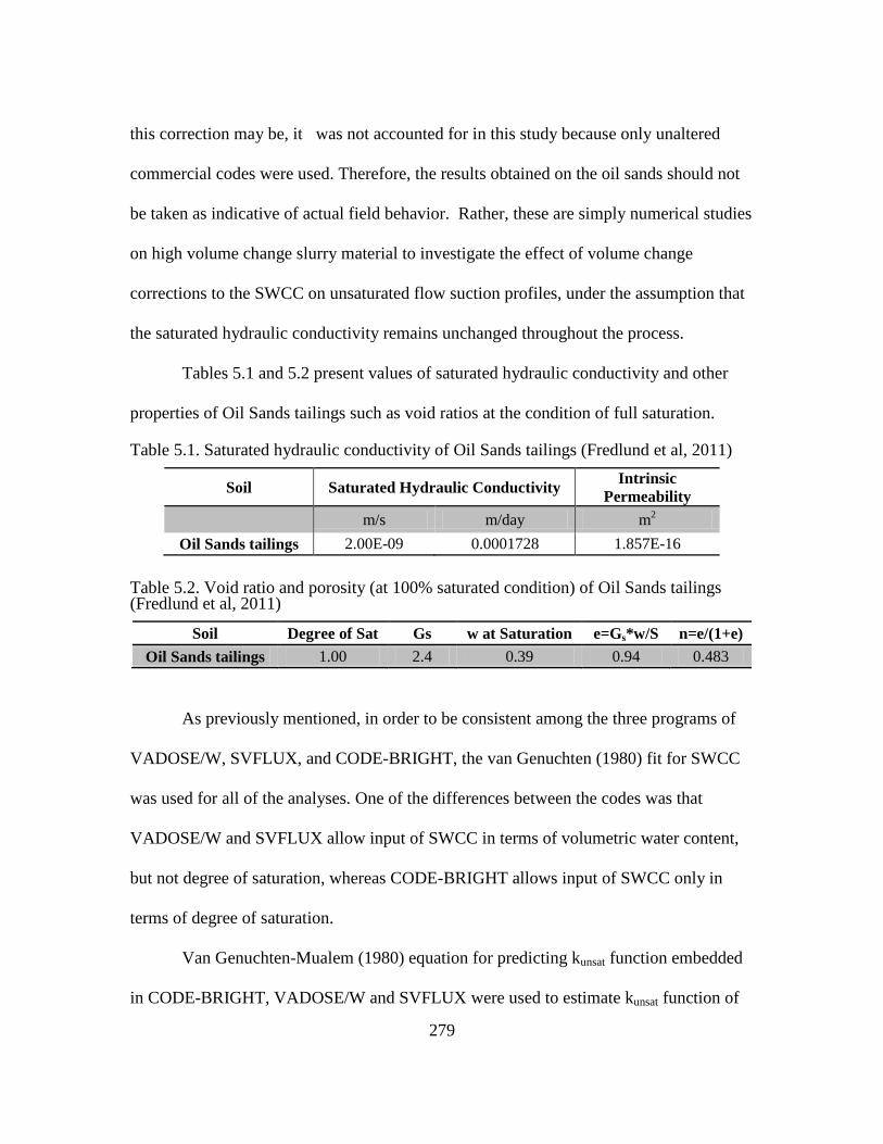
279
this correction may be, it was not accounted for in this study because only unaltered
commercial codes were used. Therefore, the results obtained on the oil sands should not
be taken as indicative of actual field behavior. Rather, these are simply numerical studies
on high volume change slurry material to investigate the effect of volume change
corrections to the SWCC on unsaturated flow suction profiles, under the assumption that
the saturated hydraulic conductivity remains unchanged throughout the process.
Tables 5.1 and 5.2 present values of saturated hydraulic conductivity and other
properties of Oil Sands tailings such as void ratios at the condition of full saturation.
Table 5.1. Saturated hydraulic conductivity of Oil Sands tailings (Fredlund et al, 2011)
Soil Saturated Hydraulic Conductivity Intrinsic
Permeability
m/s m/day m
2
Oil Sands tailings 2.00E-09 0.0001728 1.857E-16
Table 5.2. Void ratio and porosity (at 100% saturated condition) of Oil Sands tailings (Fredlund et al, 2011)
Soil Degree of Sat Gs w at Saturation e=Gs*w/S n=e/(1+e)
Oil Sands tailings 1.00 2.4 0.39 0.94 0.483
As previously mentioned, in order to be consistent among the three programs of
VADOSE/W, SVFLUX, and CODE-BRIGHT, the van Genuchten (1980) fit for SWCC
was used for all of the analyses. One of the differences between the codes was that
VADOSE/W and SVFLUX allow input of SWCC in terms of volumetric water content,
but not degree of saturation, whereas CODE-BRIGHT allows input of SWCC only in
terms of degree of saturation.
Van Genuchten-Mualem (1980) equation for predicting kunsat function embedded
in CODE-BRIGHT, VADOSE/W and SVFLUX were used to estimate kunsat function of
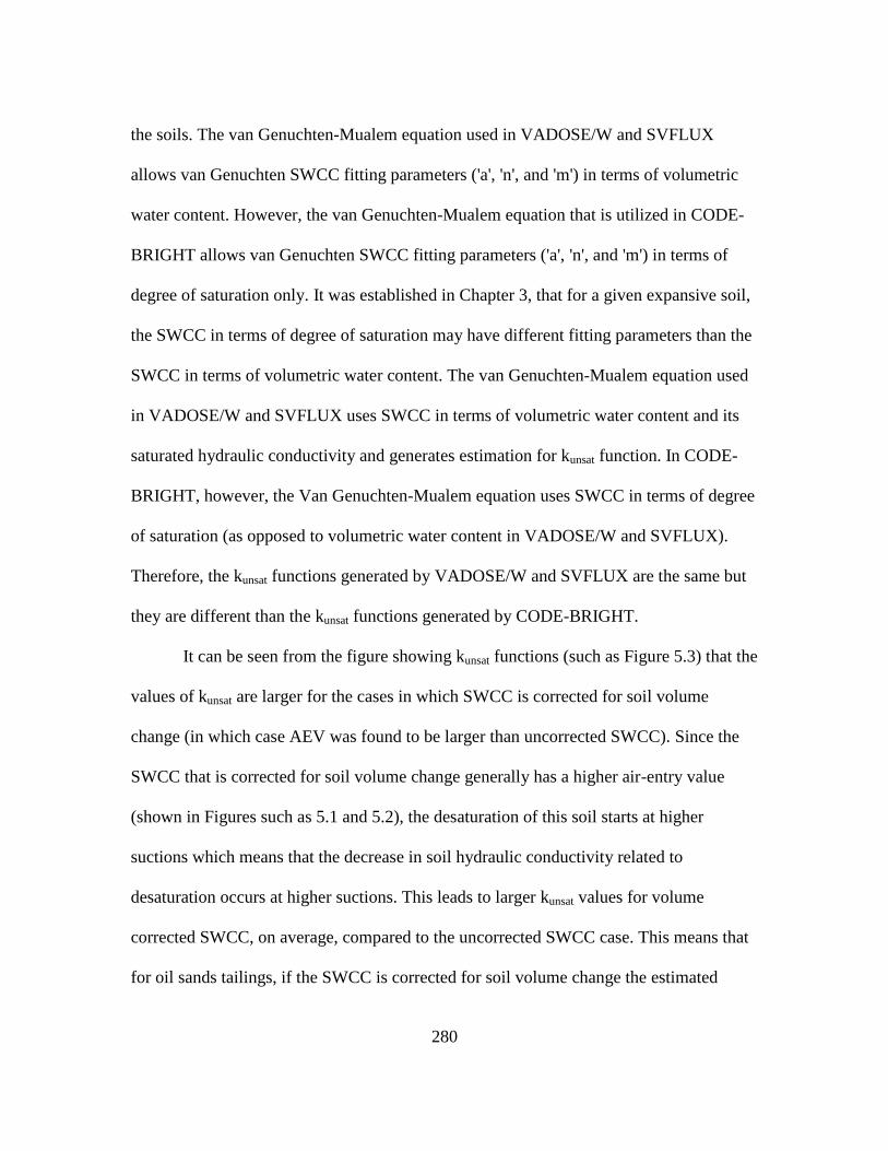
280
the soils. The van Genuchten-Mualem equation used in VADOSE/W and SVFLUX
allows van Genuchten SWCC fitting parameters ('a', 'n', and 'm') in terms of volumetric
water content. However, the van Genuchten-Mualem equation that is utilized in CODE-
BRIGHT allows van Genuchten SWCC fitting parameters ('a', 'n', and 'm') in terms of
degree of saturation only. It was established in Chapter 3, that for a given expansive soil,
the SWCC in terms of degree of saturation may have different fitting parameters than the
SWCC in terms of volumetric water content. The van Genuchten-Mualem equation used
in VADOSE/W and SVFLUX uses SWCC in terms of volumetric water content and its
saturated hydraulic conductivity and generates estimation for kunsat function. In CODE-
BRIGHT, however, the Van Genuchten-Mualem equation uses SWCC in terms of degree
of saturation (as opposed to volumetric water content in VADOSE/W and SVFLUX).
Therefore, the kunsat functions generated by VADOSE/W and SVFLUX are the same but
they are different than the kunsat functions generated by CODE-BRIGHT.
It can be seen from the figure showing kunsat functions (such as Figure 5.3) that the
values of kunsat are larger for the cases in which SWCC is corrected for soil volume
change (in which case AEV was found to be larger than uncorrected SWCC). Since the
SWCC that is corrected for soil volume change generally has a higher air-entry value
(shown in Figures such as 5.1 and 5.2), the desaturation of this soil starts at higher
suctions which means that the decrease in soil hydraulic conductivity related to
desaturation occurs at higher suctions. This leads to larger kunsat values for volume
corrected SWCC, on average, compared to the uncorrected SWCC case. This means that
for oil sands tailings, if the SWCC is corrected for soil volume change the estimated
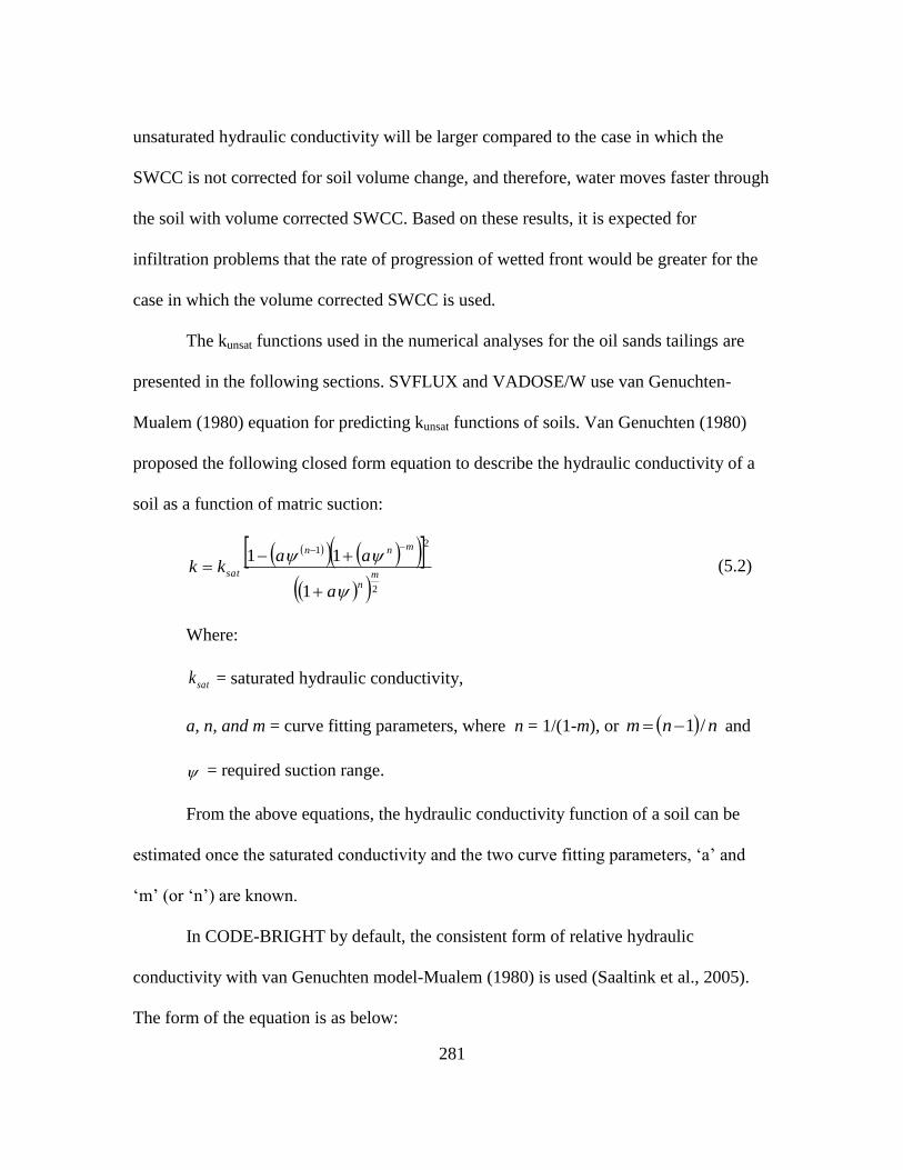
281
unsaturated hydraulic conductivity will be larger compared to the case in which the
SWCC is not corrected for soil volume change, and therefore, water moves faster through
the soil with volume corrected SWCC. Based on these results, it is expected for
infiltration problems that the rate of progression of wetted front would be greater for the
case in which the volume corrected SWCC is used.
The kunsat functions used in the numerical analyses for the oil sands tailings are
presented in the following sections. SVFLUX and VADOSE/W use van Genuchten-
Mualem (1980) equation for predicting kunsat functions of soils. Van Genuchten (1980)
proposed the following closed form equation to describe the hydraulic conductivity of a
soil as a function of matric suction:
2
21
1
11m
n
mnn
sat
a
aakk
(5.2)
Where:
satk = saturated hydraulic conductivity,
a, n, and m = curve fitting parameters, where n = 1/(1-m), or nnm /1 and
= required suction range.
From the above equations, the hydraulic conductivity function of a soil can be
estimated once the saturated conductivity and the two curve fitting parameters, ‘a’ and
‘m’ (or ‘n’) are known.
In CODE-BRIGHT by default, the consistent form of relative hydraulic
conductivity with van Genuchten model-Mualem (1980) is used (Saaltink et al., 2005).
The form of the equation is as below:
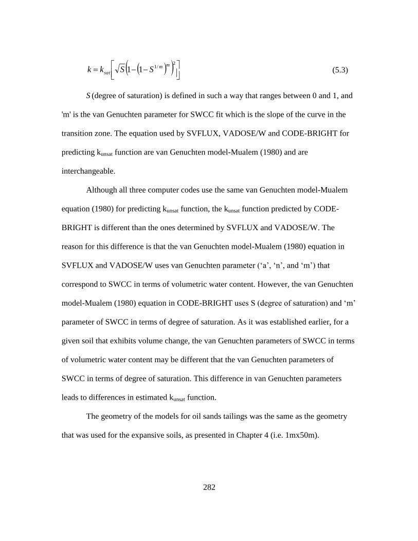
282
2/111
mm
sat SSkk (5.3)
S (degree of saturation) is defined in such a way that ranges between 0 and 1, and
'm' is the van Genuchten parameter for SWCC fit which is the slope of the curve in the
transition zone. The equation used by SVFLUX, VADOSE/W and CODE-BRIGHT for
predicting kunsat function are van Genuchten model-Mualem (1980) and are
interchangeable.
Although all three computer codes use the same van Genuchten model-Mualem
equation (1980) for predicting kunsat function, the kunsat function predicted by CODE-
BRIGHT is different than the ones determined by SVFLUX and VADOSE/W. The
reason for this difference is that the van Genuchten model-Mualem (1980) equation in
SVFLUX and VADOSE/W uses van Genuchten parameter (‘a’, ‘n’, and ‘m’) that
correspond to SWCC in terms of volumetric water content. However, the van Genuchten
model-Mualem (1980) equation in CODE-BRIGHT uses S (degree of saturation) and ‘m’
parameter of SWCC in terms of degree of saturation. As it was established earlier, for a
given soil that exhibits volume change, the van Genuchten parameters of SWCC in terms
of volumetric water content may be different that the van Genuchten parameters of
SWCC in terms of degree of saturation. This difference in van Genuchten parameters
leads to differences in estimated kunsat function.
The geometry of the models for oil sands tailings was the same as the geometry
that was used for the expansive soils, as presented in Chapter 4 (i.e. 1mx50m).

283
5.2. Properties of Oil Sands Tailings
One of the soils modeled in this study was the Oil Sands tailings studied by
Fredlund and presented in Fredlund and Houston (2013), and Fredlund et al. (2011). The
2011 article, "Interpretation of Soil-Water Characteristic Curves when Volume Change
Occurs as Soil Suction is Changed," presents properties of Oil Sands tailings which
exhibit extensive volume change upon wetting and drying.
Specific gravity of Oil Sands tailings was reported to be 2.4 and water content at
saturated condition was reported to be 39% (Fredlund and Houston, 2013, and Fredlund
et al., 2011). Therefore, at a condition of full saturation, the void ratio is calculated to be
0.936 (by using the equation of S*e=Gs*w; 100% *e= 2.4*0.39; e= 0.936).
Figures 5.1 and 5.2 show the SWCC of Oil Sands tailings in terms of volumetric
water content and degree of saturation along with van Genuchten (1980) fit. These
figures illustrate the large difference between the SWCC corrected for volume change
and SWCC uncorrected for volume change. It can be seen that for both SWCC in terms
of volumetric water content and degree of saturation, van Genuchten 'a' parameter is
larger for corrected case compared to the uncorrected. This means that the air-entry value
is higher for corrected SWCC.
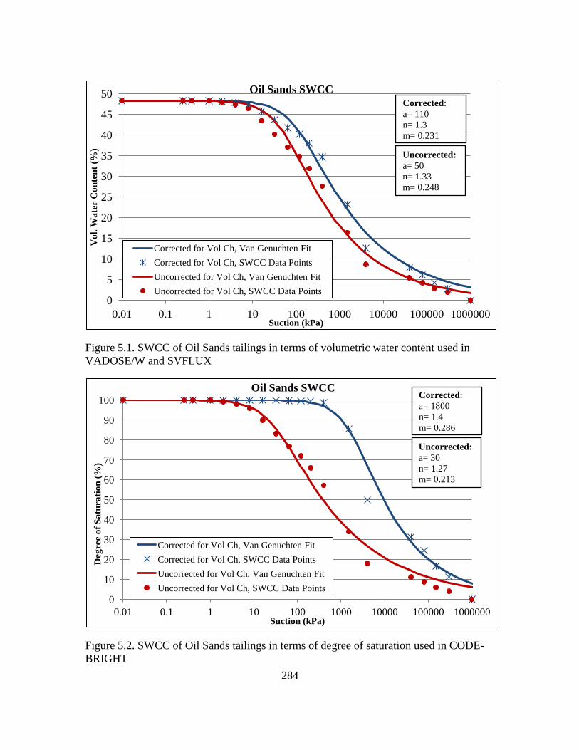
284
Figure 5.1. SWCC of Oil Sands tailings in terms of volumetric water content used in
VADOSE/W and SVFLUX
Figure 5.2. SWCC of Oil Sands tailings in terms of degree of saturation used in CODE-
BRIGHT
0
5
10
15
20
25
30
35
40
45
50
0.01 0.1 1 10 100 1000 10000 100000 1000000
Vo
l. W
ate
r C
on
ten
t (%
)
Suction (kPa)
Oil Sands SWCC
Corrected for Vol Ch, Van Genuchten Fit
Corrected for Vol Ch, SWCC Data Points
Uncorrected for Vol Ch, Van Genuchten Fit
Uncorrected for Vol Ch, SWCC Data Points
Corrected:
a= 110
n= 1.3
m= 0.231
Uncorrected:
a= 50
n= 1.33
m= 0.248
0
10
20
30
40
50
60
70
80
90
100
0.01 0.1 1 10 100 1000 10000 100000 1000000
Deg
ree
of
Sa
tura
tio
n (
%)
Suction (kPa)
Oil Sands SWCC
Corrected for Vol Ch, Van Genuchten Fit
Corrected for Vol Ch, SWCC Data Points
Uncorrected for Vol Ch, Van Genuchten Fit
Uncorrected for Vol Ch, SWCC Data Points
Corrected:
a= 1800
n= 1.4
m= 0.286
Uncorrected:
a= 30
n= 1.27
m= 0.213
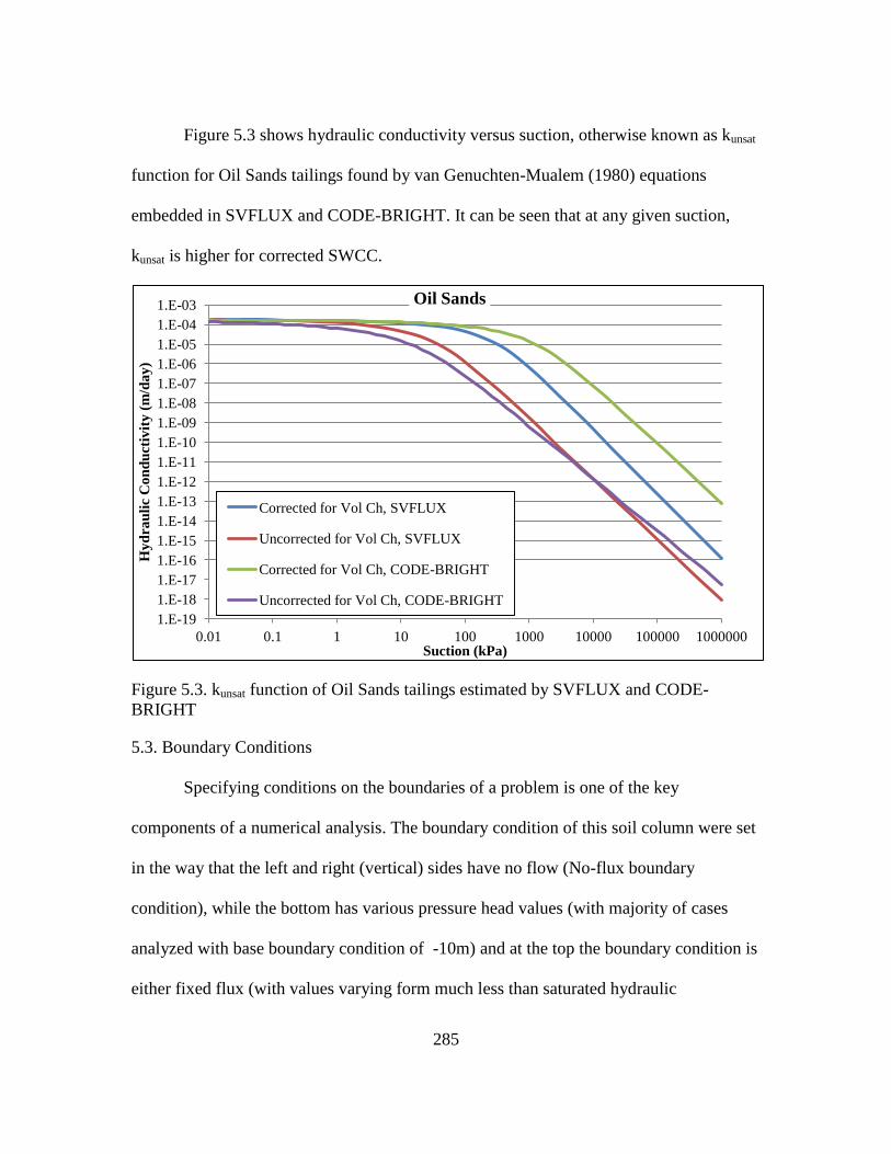
285
Figure 5.3 shows hydraulic conductivity versus suction, otherwise known as kunsat
function for Oil Sands tailings found by van Genuchten-Mualem (1980) equations
embedded in SVFLUX and CODE-BRIGHT. It can be seen that at any given suction,
kunsat is higher for corrected SWCC.
Figure 5.3. kunsat function of Oil Sands tailings estimated by SVFLUX and CODE-
BRIGHT
5.3. Boundary Conditions
Specifying conditions on the boundaries of a problem is one of the key
components of a numerical analysis. The boundary condition of this soil column were set
in the way that the left and right (vertical) sides have no flow (No-flux boundary
condition), while the bottom has various pressure head values (with majority of cases
analyzed with base boundary condition of -10m) and at the top the boundary condition is
either fixed flux (with values varying form much less than saturated hydraulic
1.E-19
1.E-18
1.E-17
1.E-16
1.E-15
1.E-14
1.E-13
1.E-12
1.E-11
1.E-10
1.E-09
1.E-08
1.E-07
1.E-06
1.E-05
1.E-04
1.E-03
0.01 0.1 1 10 100 1000 10000 100000 1000000
Hy
dra
uli
c C
on
du
ctiv
ity
(m
/da
y)
Suction (kPa)
Oil Sands
Corrected for Vol Ch, SVFLUX
Uncorrected for Vol Ch, SVFLUX
Corrected for Vol Ch, CODE-BRIGHT
Uncorrected for Vol Ch, CODE-BRIGHT
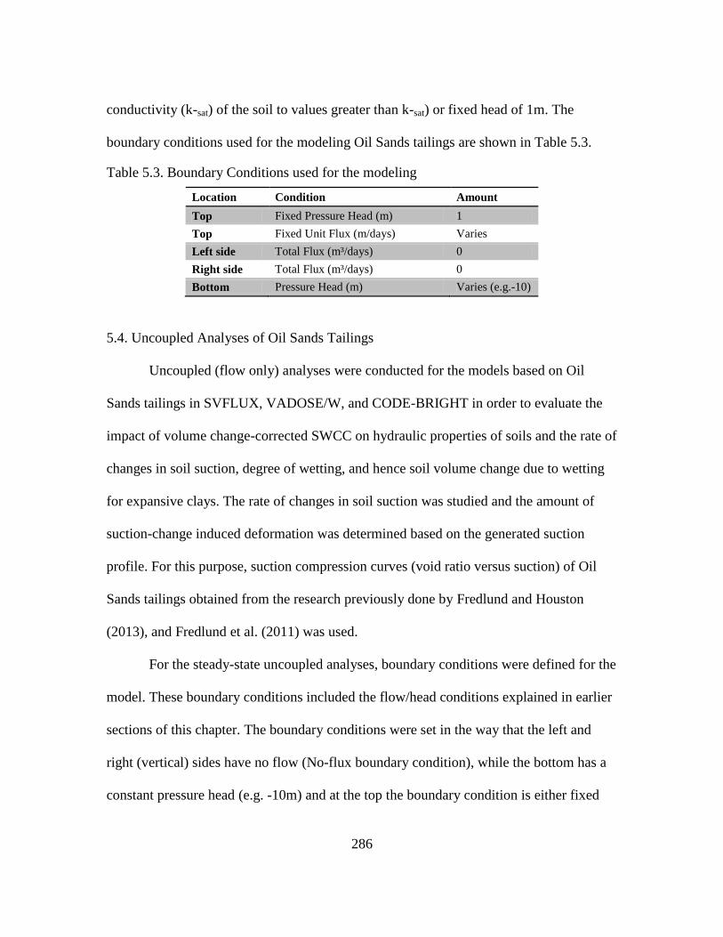
286
conductivity (k-sat) of the soil to values greater than k-sat) or fixed head of 1m. The
boundary conditions used for the modeling Oil Sands tailings are shown in Table 5.3.
Table 5.3. Boundary Conditions used for the modeling
Location Condition Amount
Top Fixed Pressure Head (m) 1
Top Fixed Unit Flux (m/days) Varies
Left side Total Flux (m³/days) 0
Right side Total Flux (m³/days) 0
Bottom Pressure Head (m) Varies (e.g.-10)
5.4. Uncoupled Analyses of Oil Sands Tailings
Uncoupled (flow only) analyses were conducted for the models based on Oil
Sands tailings in SVFLUX, VADOSE/W, and CODE-BRIGHT in order to evaluate the
impact of volume change-corrected SWCC on hydraulic properties of soils and the rate of
changes in soil suction, degree of wetting, and hence soil volume change due to wetting
for expansive clays. The rate of changes in soil suction was studied and the amount of
suction-change induced deformation was determined based on the generated suction
profile. For this purpose, suction compression curves (void ratio versus suction) of Oil
Sands tailings obtained from the research previously done by Fredlund and Houston
(2013), and Fredlund et al. (2011) was used.
For the steady-state uncoupled analyses, boundary conditions were defined for the
model. These boundary conditions included the flow/head conditions explained in earlier
sections of this chapter. The boundary conditions were set in the way that the left and
right (vertical) sides have no flow (No-flux boundary condition), while the bottom has a
constant pressure head (e.g. -10m) and at the top the boundary condition is either fixed
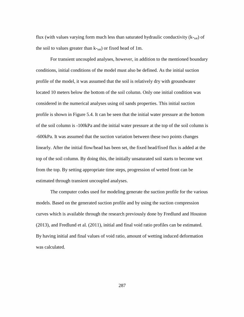
287
flux (with values varying form much less than saturated hydraulic conductivity (k-sat) of
the soil to values greater than k-sat) or fixed head of 1m.
For transient uncoupled analyses, however, in addition to the mentioned boundary
conditions, initial conditions of the model must also be defined. As the initial suction
profile of the model, it was assumed that the soil is relatively dry with groundwater
located 10 meters below the bottom of the soil column. Only one initial condition was
considered in the numerical analyses using oil sands properties. This initial suction
profile is shown in Figure 5.4. It can be seen that the initial water pressure at the bottom
of the soil column is -100kPa and the initial water pressure at the top of the soil column is
-600kPa. It was assumed that the suction variation between these two points changes
linearly. After the initial flow/head has been set, the fixed head/fixed flux is added at the
top of the soil column. By doing this, the initially unsaturated soil starts to become wet
from the top. By setting appropriate time steps, progression of wetted front can be
estimated through transient uncoupled analyses.
The computer codes used for modeling generate the suction profile for the various
models. Based on the generated suction profile and by using the suction compression
curves which is available through the research previously done by Fredlund and Houston
(2013), and Fredlund et al. (2011), initial and final void ratio profiles can be estimated.
By having initial and final values of void ratio, amount of wetting induced deformation
was calculated.
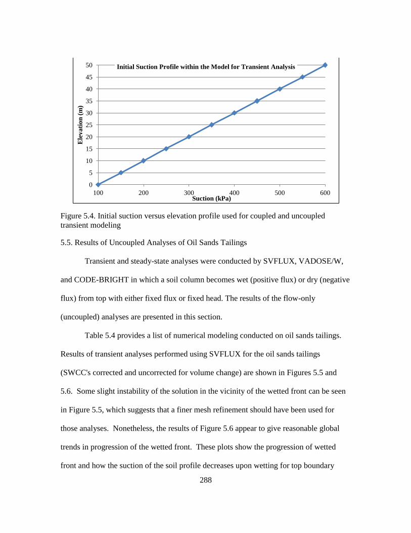
288
Figure 5.4. Initial suction versus elevation profile used for coupled and uncoupled
transient modeling
5.5. Results of Uncoupled Analyses of Oil Sands Tailings
Transient and steady-state analyses were conducted by SVFLUX, VADOSE/W,
and CODE-BRIGHT in which a soil column becomes wet (positive flux) or dry (negative
flux) from top with either fixed flux or fixed head. The results of the flow-only
(uncoupled) analyses are presented in this section.
Table 5.4 provides a list of numerical modeling conducted on oil sands tailings.
Results of transient analyses performed using SVFLUX for the oil sands tailings
(SWCC's corrected and uncorrected for volume change) are shown in Figures 5.5 and
5.6. Some slight instability of the solution in the vicinity of the wetted front can be seen
in Figure 5.5, which suggests that a finer mesh refinement should have been used for
those analyses. Nonetheless, the results of Figure 5.6 appear to give reasonable global
trends in progression of the wetted front. These plots show the progression of wetted
front and how the suction of the soil profile decreases upon wetting for top boundary
0
5
10
15
20
25
30
35
40
45
50
100 200 300 400 500 600
Ele
va
tio
n (
m)
Suction (kPa)
Initial Suction Profile within the Model for Transient Analysis
289
condition of fixed flux of 2e-4 m/day (slightly larger than ksat). It can be seen that in the
case with corrected SWCC, the soil gets wet quicker (faster rate of progression of wetted
front). This is due to the fact that the unsaturated hydraulic conductivity of the soil with
corrected SWCC is higher than that of uncorrected SWCC. The kunsat functions of oil
sands tailings were presented earlier in this chapter and it was found that the kunsat values
are generally greater for volume corrected SWCC's compared to uncorrected SWCC's.
Higher values of kunsat result in water penetrating through the soil faster than for the case
in which values of kunsat are lower. Figure 5.7 can be used to compare the final (steady-
state condition) of the suction within the soil profile for the two cases of SWCC corrected
and uncorrected for soil volume change. This condition corresponds to the long-enough
time since the start of the top fixed flux, so that the soil profile has become saturated. It
can be seen that although for both cases, the soil has become fully wetted; the overall
suction of the soil is smaller (i.e. larger water pressure values) for the case in which
SWCC is uncorrected for soil volume change.
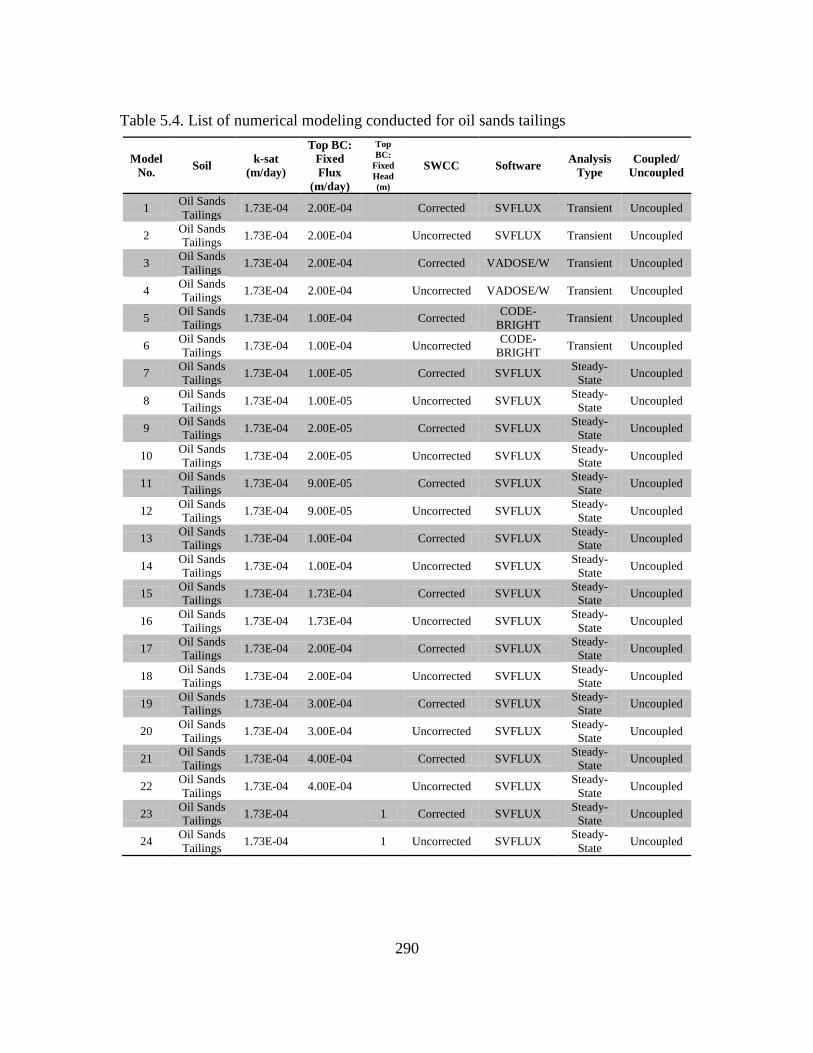
290
Table 5.4. List of numerical modeling conducted for oil sands tailings
Model
No. Soil
k-sat
(m/day)
Top BC:
Fixed
Flux
(m/day)
Top
BC:
Fixed
Head
(m)
SWCC Software Analysis
Type
Coupled/
Uncoupled
1 Oil Sands
Tailings 1.73E-04 2.00E-04
Corrected SVFLUX Transient Uncoupled
2 Oil Sands
Tailings 1.73E-04 2.00E-04
Uncorrected SVFLUX Transient Uncoupled
3 Oil Sands
Tailings 1.73E-04 2.00E-04
Corrected VADOSE/W Transient Uncoupled
4 Oil Sands
Tailings 1.73E-04 2.00E-04
Uncorrected VADOSE/W Transient Uncoupled
5 Oil Sands
Tailings 1.73E-04 1.00E-04
Corrected
CODE-
BRIGHT Transient Uncoupled
6 Oil Sands
Tailings 1.73E-04 1.00E-04
Uncorrected
CODE-
BRIGHT Transient Uncoupled
7 Oil Sands
Tailings 1.73E-04 1.00E-05
Corrected SVFLUX
Steady-
State Uncoupled
8 Oil Sands
Tailings 1.73E-04 1.00E-05
Uncorrected SVFLUX
Steady-
State Uncoupled
9 Oil Sands
Tailings 1.73E-04 2.00E-05
Corrected SVFLUX
Steady-
State Uncoupled
10 Oil Sands
Tailings 1.73E-04 2.00E-05
Uncorrected SVFLUX
Steady-
State Uncoupled
11 Oil Sands
Tailings 1.73E-04 9.00E-05
Corrected SVFLUX
Steady-
State Uncoupled
12 Oil Sands
Tailings 1.73E-04 9.00E-05
Uncorrected SVFLUX
Steady-
State Uncoupled
13 Oil Sands
Tailings 1.73E-04 1.00E-04
Corrected SVFLUX
Steady-
State Uncoupled
14 Oil Sands
Tailings 1.73E-04 1.00E-04
Uncorrected SVFLUX
Steady-
State Uncoupled
15 Oil Sands
Tailings 1.73E-04 1.73E-04
Corrected SVFLUX
Steady-
State Uncoupled
16 Oil Sands
Tailings 1.73E-04 1.73E-04
Uncorrected SVFLUX
Steady-
State Uncoupled
17 Oil Sands
Tailings 1.73E-04 2.00E-04
Corrected SVFLUX
Steady-
State Uncoupled
18 Oil Sands
Tailings 1.73E-04 2.00E-04
Uncorrected SVFLUX
Steady-
State Uncoupled
19 Oil Sands
Tailings 1.73E-04 3.00E-04
Corrected SVFLUX
Steady-
State Uncoupled
20 Oil Sands
Tailings 1.73E-04 3.00E-04
Uncorrected SVFLUX
Steady-
State Uncoupled
21 Oil Sands
Tailings 1.73E-04 4.00E-04
Corrected SVFLUX
Steady-
State Uncoupled
22 Oil Sands
Tailings 1.73E-04 4.00E-04
Uncorrected SVFLUX
Steady-
State Uncoupled
23 Oil Sands
Tailings 1.73E-04
1 Corrected SVFLUX
Steady-
State Uncoupled
24 Oil Sands
Tailings 1.73E-04
1 Uncorrected SVFLUX
Steady-
State Uncoupled
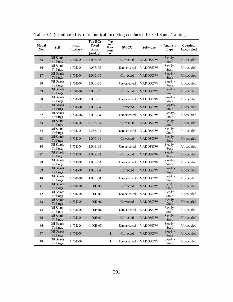
291
Table 5.4. (Continue) List of numerical modeling conducted for Oil Sands Tailings
Model
No. Soil
k-sat
(m/day)
Top BC:
Fixed
Flux
(m/day)
Top
BC:
Fixed
Head
(m)
SWCC Software Analysis
Type
Coupled/
Uncoupled
25 Oil Sands
Tailings 1.73E-04 1.00E-05
Corrected VADOSE/W
Steady-
State Uncoupled
26 Oil Sands
Tailings 1.73E-04 1.00E-05
Uncorrected VADOSE/W
Steady-
State Uncoupled
27 Oil Sands
Tailings 1.73E-04 2.00E-05
Corrected VADOSE/W
Steady-
State Uncoupled
28 Oil Sands
Tailings 1.73E-04 2.00E-05
Uncorrected VADOSE/W
Steady-
State Uncoupled
29 Oil Sands
Tailings 1.73E-04 9.00E-05
Corrected VADOSE/W
Steady-
State Uncoupled
30 Oil Sands
Tailings 1.73E-04 9.00E-05
Uncorrected VADOSE/W
Steady-
State Uncoupled
31 Oil Sands
Tailings 1.73E-04 1.00E-04
Corrected VADOSE/W
Steady-
State Uncoupled
32 Oil Sands
Tailings 1.73E-04 1.00E-04
Uncorrected VADOSE/W
Steady-
State Uncoupled
33 Oil Sands
Tailings 1.73E-04 1.73E-04
Corrected VADOSE/W
Steady-
State Uncoupled
34 Oil Sands
Tailings 1.73E-04 1.73E-04
Uncorrected VADOSE/W
Steady-
State Uncoupled
35 Oil Sands
Tailings 1.73E-04 2.00E-04
Corrected VADOSE/W
Steady-
State Uncoupled
36 Oil Sands
Tailings 1.73E-04 2.00E-04
Uncorrected VADOSE/W
Steady-
State Uncoupled
37 Oil Sands
Tailings 1.73E-04 3.00E-04
Corrected VADOSE/W
Steady-
State Uncoupled
38 Oil Sands
Tailings 1.73E-04 3.00E-04
Uncorrected VADOSE/W
Steady-
State Uncoupled
39 Oil Sands
Tailings 1.73E-04 4.00E-04
Corrected VADOSE/W
Steady-
State Uncoupled
40 Oil Sands
Tailings 1.73E-04 4.00E-04
Uncorrected VADOSE/W
Steady-
State Uncoupled
41 Oil Sands
Tailings 1.73E-04 -1.00E-05
Corrected VADOSE/W
Steady-
State Uncoupled
42 Oil Sands
Tailings 1.73E-04 -1.00E-05
Uncorrected VADOSE/W
Steady-
State Uncoupled
43 Oil Sands
Tailings 1.73E-04 -1.00E-06
Corrected VADOSE/W
Steady-
State Uncoupled
44 Oil Sands
Tailings 1.73E-04 -1.00E-06
Uncorrected VADOSE/W
Steady-
State Uncoupled
45 Oil Sands
Tailings 1.73E-04 -1.00E-07
Corrected VADOSE/W
Steady-
State Uncoupled
46 Oil Sands
Tailings 1.73E-04 -1.00E-07
Uncorrected VADOSE/W
Steady-
State Uncoupled
47 Oil Sands
Tailings 1.73E-04
1 Corrected VADOSE/W
Steady-
State Uncoupled
48 Oil Sands
Tailings 1.73E-04
1 Uncorrected VADOSE/W
Steady-
State Uncoupled
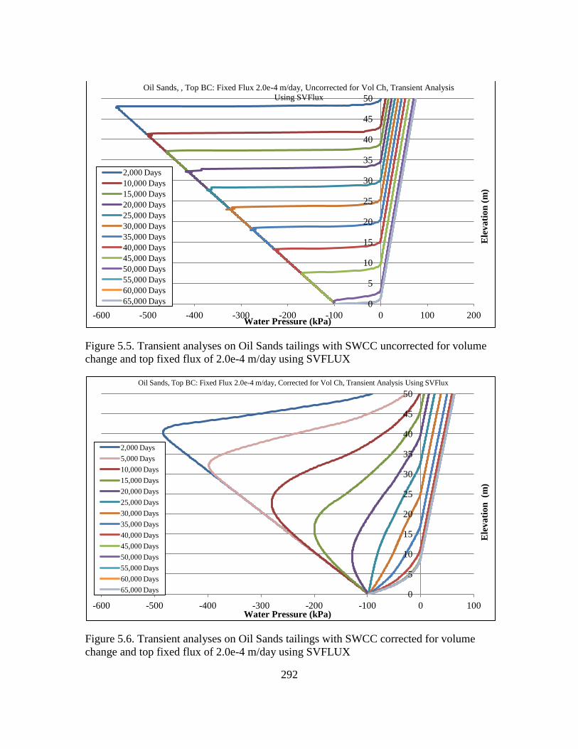
292
Figure 5.5. Transient analyses on Oil Sands tailings with SWCC uncorrected for volume
change and top fixed flux of 2.0e-4 m/day using SVFLUX
Figure 5.6. Transient analyses on Oil Sands tailings with SWCC corrected for volume
change and top fixed flux of 2.0e-4 m/day using SVFLUX
0
5
10
15
20
25
30
35
40
45
50
-600 -500 -400 -300 -200 -100 0 100 200
Ele
va
tio
n (
m)
Water Pressure (kPa)
Oil Sands, , Top BC: Fixed Flux 2.0e-4 m/day, Uncorrected for Vol Ch, Transient Analysis
Using SVFlux
2,000 Days
10,000 Days
15,000 Days
20,000 Days
25,000 Days
30,000 Days
35,000 Days
40,000 Days
45,000 Days
50,000 Days
55,000 Days
60,000 Days
65,000 Days
0
5
10
15
20
25
30
35
40
45
50
-600 -500 -400 -300 -200 -100 0 100
Ele
va
tio
n (m
)
Water Pressure (kPa)
Oil Sands, Top BC: Fixed Flux 2.0e-4 m/day, Corrected for Vol Ch, Transient Analysis Using SVFlux
2,000 Days
5,000 Days
10,000 Days
15,000 Days
20,000 Days
25,000 Days
30,000 Days
35,000 Days
40,000 Days
45,000 Days
50,000 Days
55,000 Days
60,000 Days
65,000 Days
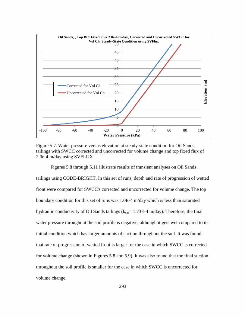
293
Figure 5.7. Water pressure versus elevation at steady-state condition for Oil Sands
tailings with SWCC corrected and uncorrected for volume change and top fixed flux of
2.0e-4 m/day using SVFLUX
Figures 5.8 through 5.11 illustrate results of transient analyses on Oil Sands
tailings using CODE-BRIGHT. In this set of runs, depth and rate of progression of wetted
front were compared for SWCC's corrected and uncorrected for volume change. The top
boundary condition for this set of runs was 1.0E-4 m/day which is less than saturated
hydraulic conductivity of Oil Sands tailings (ksat= 1.73E-4 m/day). Therefore, the final
water pressure throughout the soil profile is negative, although it gets wet compared to its
initial condition which has larger amounts of suction throughout the soil. It was found
that rate of progression of wetted front is larger for the case in which SWCC is corrected
for volume change (shown in Figures 5.8 and 5.9). It was also found that the final suction
throughout the soil profile is smaller for the case in which SWCC is uncorrected for
volume change.
0
5
10
15
20
25
30
35
40
45
50
-100 -80 -60 -40 -20 0 20 40 60 80 100
Ele
va
tio
n (m
)
Water Pressure (kPa)
Oil Sands, , Top BC: Fixed Flux 2.0e-4 m/day, Corrected and Uncorrected SWCC for
Vol Ch, Steady-State Condition using SVFlux
Corrected for Vol Ch
Uncorrected for Vol Ch
294
Initial condition of the soil is unsaturated with suction of 100kPa at the bottom
and suction of 600kPa at the top of the model. When the soil becomes wet from the top
by adding the fixed flux, the suction of soil starts to decrease. In other words, the wetting
path on the SWCC will be followed when the soil becomes wet. It was previously
established that the volume corrected SWCC generally has larger air-entry value
compared to the uncorrected SWCC. This means that in the soil with volume corrected
SWCC, desaturation starts at a larger suction compared to the soil with uncorrected
SWCC. That is to say, the soil with corrected SWCC stays saturated at larger suction
ranges compared to the soil with uncorrected SWCC. Therefore, once the soil becomes
wet and the suction decreases (i.e. wetting path on the SWCC), for the soil with corrected
SWCC, the soil becomes saturated at a larger suction (close to air-entry value). Whereas,
the suction within the soil with uncorrected SWCC should further decrease (compared to
the soil with corrected SWCC) in order for the soil to reach the air-entry value (saturated
condition). This mechanism illustrates the reason for the difference in generated suction
values for the cases of volume corrected SWCC and volume uncorrected SWCC. It
should be mentioned that for a certain expansive soil, the smaller final suction within the
soil profile indicates larger deformation. This is due to the general shape of suction
compression curves, in which the void ratio of the expansive soils is larger at smaller
suction values. The soil deformations calculated using the final suction profile of the soil
and its suction compression curve are described later in this chapter.
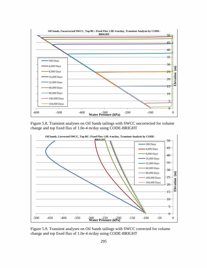
295
Figure 5.8. Transient analyses on Oil Sands tailings with SWCC uncorrected for volume
change and top fixed flux of 1.0e-4 m/day using CODE-BRIGHT
Figure 5.9. Transient analyses on Oil Sands tailings with SWCC corrected for volume
change and top fixed flux of 1.0e-4 m/day using CODE-BRIGHT
0
5
10
15
20
25
30
35
40
45
50
-600 -500 -400 -300 -200 -100 0
Ele
va
tio
n (m
)
Water Pressure (kPa)
Oil Sands, Uncorrected SWCC, Top BC: Fixed Flux 1.0E-4 m/day, Transient Analysis by CODE-
BRIGHT
500 Days
4,000 Days
8,000 Days
16,000 Days
32,000 Days
60,000 Days
80,000 Days
100,000 Days
104,000 Days
0
5
10
15
20
25
30
35
40
45
50
-500 -450 -400 -350 -300 -250 -200 -150 -100 -50 0
Ele
va
tio
n (m
)
Water Pressure (kPa)
Oil Sands, Corrected SWCC, Top BC: Fixed Flux 1.0E-4 m/day, Transient Analysis by CODE-
BRIGHT
500 Days
4,000 Days
8,000 Days
16,000 Days
32,000 Days
60,000 Days
80,000 Days
100,000 Days
104,000 Days
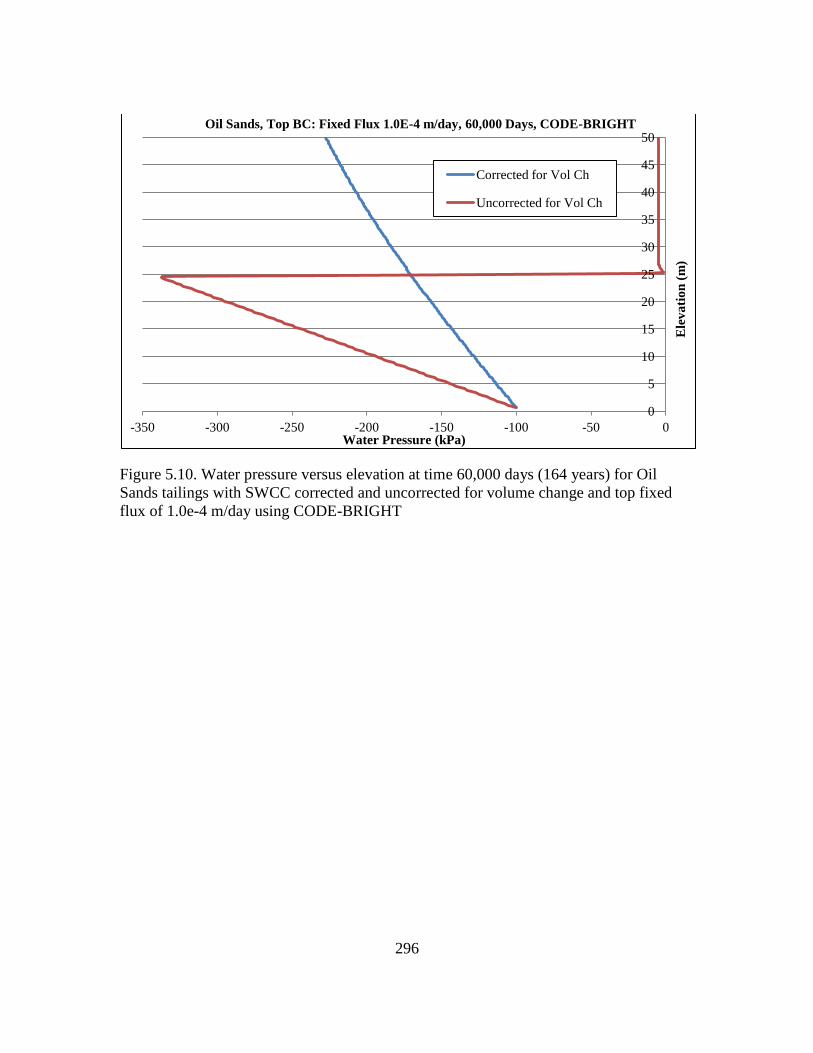
296
Figure 5.10. Water pressure versus elevation at time 60,000 days (164 years) for Oil
Sands tailings with SWCC corrected and uncorrected for volume change and top fixed
flux of 1.0e-4 m/day using CODE-BRIGHT
0
5
10
15
20
25
30
35
40
45
50
-350 -300 -250 -200 -150 -100 -50 0
Ele
va
tio
n (
m)
Water Pressure (kPa)
Oil Sands, Top BC: Fixed Flux 1.0E-4 m/day, 60,000 Days, CODE-BRIGHT
Corrected for Vol Ch
Uncorrected for Vol Ch
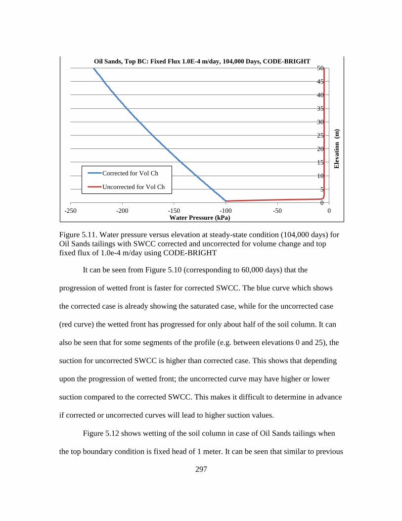
297
Figure 5.11. Water pressure versus elevation at steady-state condition (104,000 days) for
Oil Sands tailings with SWCC corrected and uncorrected for volume change and top
fixed flux of 1.0e-4 m/day using CODE-BRIGHT
It can be seen from Figure 5.10 (corresponding to 60,000 days) that the
progression of wetted front is faster for corrected SWCC. The blue curve which shows
the corrected case is already showing the saturated case, while for the uncorrected case
(red curve) the wetted front has progressed for only about half of the soil column. It can
also be seen that for some segments of the profile (e.g. between elevations 0 and 25), the
suction for uncorrected SWCC is higher than corrected case. This shows that depending
upon the progression of wetted front; the uncorrected curve may have higher or lower
suction compared to the corrected SWCC. This makes it difficult to determine in advance
if corrected or uncorrected curves will lead to higher suction values.
Figure 5.12 shows wetting of the soil column in case of Oil Sands tailings when
the top boundary condition is fixed head of 1 meter. It can be seen that similar to previous
0
5
10
15
20
25
30
35
40
45
50
-250 -200 -150 -100 -50 0
Ele
va
tio
n (m
)
Water Pressure (kPa)
Oil Sands, Top BC: Fixed Flux 1.0E-4 m/day, 104,000 Days, CODE-BRIGHT
Corrected for Vol Ch
Uncorrected for Vol Ch
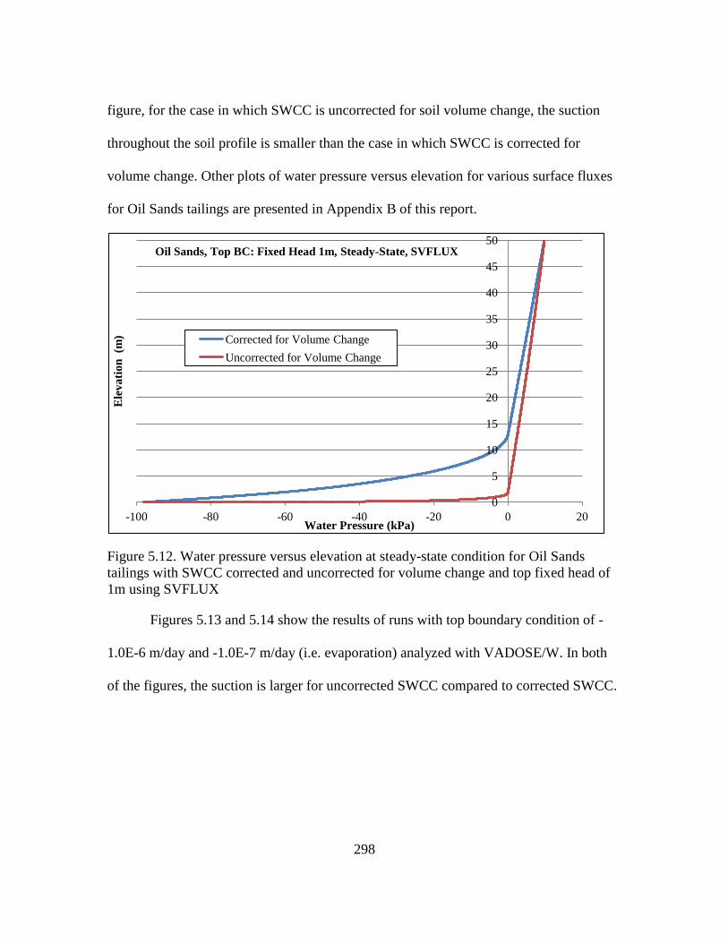
298
figure, for the case in which SWCC is uncorrected for soil volume change, the suction
throughout the soil profile is smaller than the case in which SWCC is corrected for
volume change. Other plots of water pressure versus elevation for various surface fluxes
for Oil Sands tailings are presented in Appendix B of this report.
Figure 5.12. Water pressure versus elevation at steady-state condition for Oil Sands
tailings with SWCC corrected and uncorrected for volume change and top fixed head of
1m using SVFLUX
Figures 5.13 and 5.14 show the results of runs with top boundary condition of -
1.0E-6 m/day and -1.0E-7 m/day (i.e. evaporation) analyzed with VADOSE/W. In both
of the figures, the suction is larger for uncorrected SWCC compared to corrected SWCC.
0
5
10
15
20
25
30
35
40
45
50
-100 -80 -60 -40 -20 0 20
Ele
va
tio
n (m
)
Water Pressure (kPa)
Oil Sands, Top BC: Fixed Head 1m, Steady-State, SVFLUX
Corrected for Volume Change
Uncorrected for Volume Change
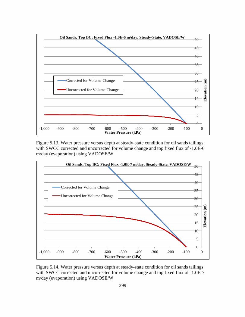
299
Figure 5.13. Water pressure versus depth at steady-state condition for oil sands tailings
with SWCC corrected and uncorrected for volume change and top fixed flux of -1.0E-6
m/day (evaporation) using VADOSE/W
Figure 5.14. Water pressure versus depth at steady-state condition for oil sands tailings
with SWCC corrected and uncorrected for volume change and top fixed flux of -1.0E-7
m/day (evaporation) using VADOSE/W
0
5
10
15
20
25
30
35
40
45
50
-1,000 -900 -800 -700 -600 -500 -400 -300 -200 -100 0
Ele
va
tio
n (
m)
Water Pressure (kPa)
Oil Sands, Top BC: Fixed Flux -1.0E-6 m/day, Steady-State, VADOSE/W
Corrected for Volume Change
Uncorrected for Volume Change
0
5
10
15
20
25
30
35
40
45
50
-1,000 -900 -800 -700 -600 -500 -400 -300 -200 -100 0
Ele
va
tio
n (
m)
Water Pressure (kPa)
Oil Sands, Top BC: Fixed Flux -1.0E-7 m/day, Steady-State, VADOSE/W
Corrected for Volume Change
Uncorrected for Volume Change
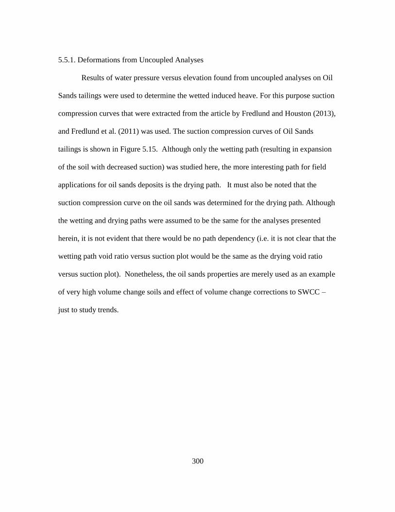
300
5.5.1. Deformations from Uncoupled Analyses
Results of water pressure versus elevation found from uncoupled analyses on Oil
Sands tailings were used to determine the wetted induced heave. For this purpose suction
compression curves that were extracted from the article by Fredlund and Houston (2013),
and Fredlund et al. (2011) was used. The suction compression curves of Oil Sands
tailings is shown in Figure 5.15. Although only the wetting path (resulting in expansion
of the soil with decreased suction) was studied here, the more interesting path for field
applications for oil sands deposits is the drying path. It must also be noted that the
suction compression curve on the oil sands was determined for the drying path. Although
the wetting and drying paths were assumed to be the same for the analyses presented
herein, it is not evident that there would be no path dependency (i.e. it is not clear that the
wetting path void ratio versus suction plot would be the same as the drying void ratio
versus suction plot). Nonetheless, the oil sands properties are merely used as an example
of very high volume change soils and effect of volume change corrections to SWCC –
just to study trends.
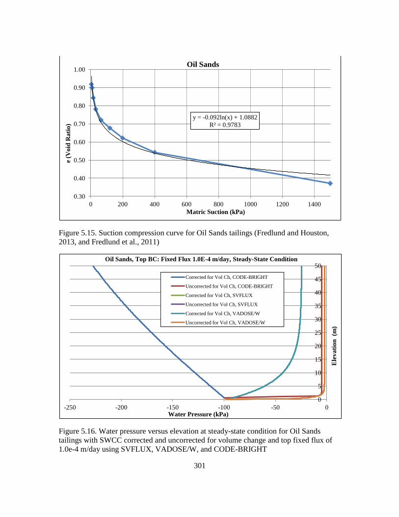
301
Figure 5.15. Suction compression curve for Oil Sands tailings (Fredlund and Houston,
2013, and Fredlund et al., 2011)
Figure 5.16. Water pressure versus elevation at steady-state condition for Oil Sands
tailings with SWCC corrected and uncorrected for volume change and top fixed flux of
1.0e-4 m/day using SVFLUX, VADOSE/W, and CODE-BRIGHT
y = -0.092ln(x) + 1.0882
R² = 0.9783
0.30
0.40
0.50
0.60
0.70
0.80
0.90
1.00
0 200 400 600 800 1000 1200 1400
e (V
oid
Ra
tio
)
Matric Suction (kPa)
Oil Sands
0
5
10
15
20
25
30
35
40
45
50
-250 -200 -150 -100 -50 0
Ele
va
tio
n (m
)
Water Pressure (kPa)
Oil Sands, Top BC: Fixed Flux 1.0E-4 m/day, Steady-State Condition
Corrected for Vol Ch, CODE-BRIGHT
Uncorrected for Vol Ch, CODE-BRIGHT
Corrected for Vol Ch, SVFLUX
Uncorrected for Vol Ch, SVFLUX
Corrected for Vol Ch, VADOSE/W
Uncorrected for Vol Ch, VADOSE/W
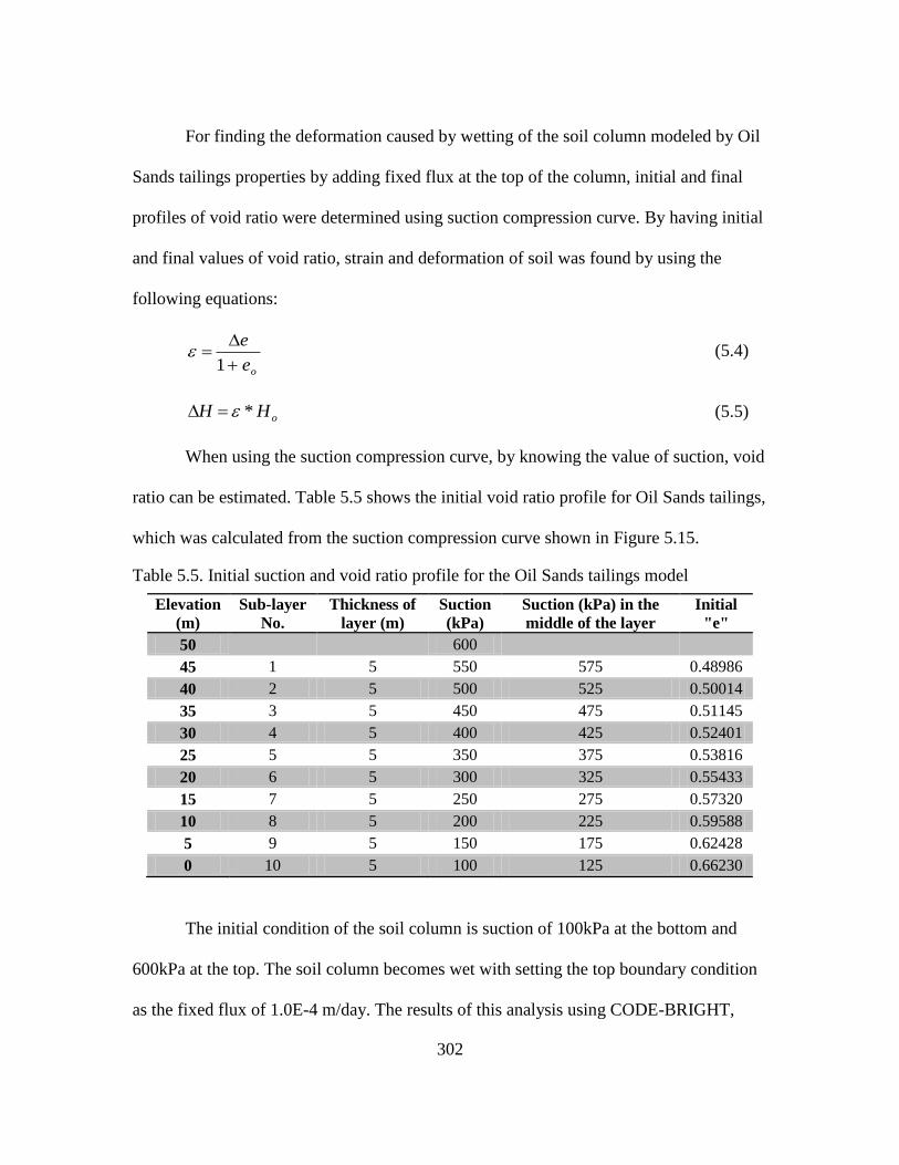
302
For finding the deformation caused by wetting of the soil column modeled by Oil
Sands tailings properties by adding fixed flux at the top of the column, initial and final
profiles of void ratio were determined using suction compression curve. By having initial
and final values of void ratio, strain and deformation of soil was found by using the
following equations:
oe
e
1 (5.4)
oHH * (5.5)
When using the suction compression curve, by knowing the value of suction, void
ratio can be estimated. Table 5.5 shows the initial void ratio profile for Oil Sands tailings,
which was calculated from the suction compression curve shown in Figure 5.15.
Table 5.5. Initial suction and void ratio profile for the Oil Sands tailings model
Elevation
(m)
Sub-layer
No.
Thickness of
layer (m)
Suction
(kPa)
Suction (kPa) in the
middle of the layer
Initial
"e"
50
600
45 1 5 550 575 0.48986
40 2 5 500 525 0.50014
35 3 5 450 475 0.51145
30 4 5 400 425 0.52401
25 5 5 350 375 0.53816
20 6 5 300 325 0.55433
15 7 5 250 275 0.57320
10 8 5 200 225 0.59588
5 9 5 150 175 0.62428
0 10 5 100 125 0.66230
The initial condition of the soil column is suction of 100kPa at the bottom and
600kPa at the top. The soil column becomes wet with setting the top boundary condition
as the fixed flux of 1.0E-4 m/day. The results of this analysis using CODE-BRIGHT,
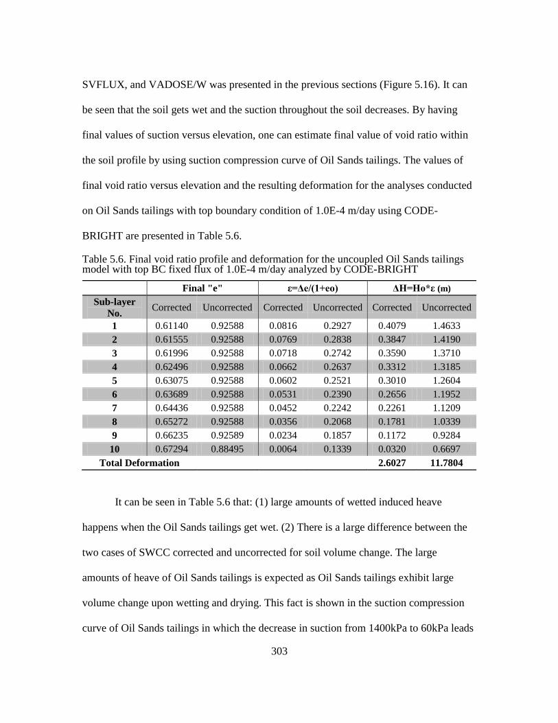
303
SVFLUX, and VADOSE/W was presented in the previous sections (Figure 5.16). It can
be seen that the soil gets wet and the suction throughout the soil decreases. By having
final values of suction versus elevation, one can estimate final value of void ratio within
the soil profile by using suction compression curve of Oil Sands tailings. The values of
final void ratio versus elevation and the resulting deformation for the analyses conducted
on Oil Sands tailings with top boundary condition of 1.0E-4 m/day using CODE-
BRIGHT are presented in Table 5.6.
Table 5.6. Final void ratio profile and deformation for the uncoupled Oil Sands tailings model with top BC fixed flux of 1.0E-4 m/day analyzed by CODE-BRIGHT
Final "e" ε=Δe/(1+eo) ΔH=Ho*ε (m)
Sub-layer
No. Corrected Uncorrected Corrected Uncorrected Corrected Uncorrected
1 0.61140 0.92588 0.0816 0.2927 0.4079 1.4633
2 0.61555 0.92588 0.0769 0.2838 0.3847 1.4190
3 0.61996 0.92588 0.0718 0.2742 0.3590 1.3710
4 0.62496 0.92588 0.0662 0.2637 0.3312 1.3185
5 0.63075 0.92588 0.0602 0.2521 0.3010 1.2604
6 0.63689 0.92588 0.0531 0.2390 0.2656 1.1952
7 0.64436 0.92588 0.0452 0.2242 0.2261 1.1209
8 0.65272 0.92588 0.0356 0.2068 0.1781 1.0339
9 0.66235 0.92589 0.0234 0.1857 0.1172 0.9284
10 0.67294 0.88495 0.0064 0.1339 0.0320 0.6697
Total Deformation
2.6027 11.7804
It can be seen in Table 5.6 that: (1) large amounts of wetted induced heave
happens when the Oil Sands tailings get wet. (2) There is a large difference between the
two cases of SWCC corrected and uncorrected for soil volume change. The large
amounts of heave of Oil Sands tailings is expected as Oil Sands tailings exhibit large
volume change upon wetting and drying. This fact is shown in the suction compression
curve of Oil Sands tailings in which the decrease in suction from 1400kPa to 60kPa leads
304
to increase in void ratio from around 0.35 to 0.72 (i.e. increase of 0.37 in void ratio). This
large amount of increase in void ratio leads to large amounts of strain and thus heaves.
As shown in Figure 5.16, the final suction profile of the case in which SWCC is
uncorrected is much smaller than the suction within the Oil Sands tailings in case of
corrected SWCC. By using the same suction compression curve, much larger final void
ratio profile for the case with uncorrected SWCC is found compared to the case in which
SWCC is corrected. Larger final void ratio throughout the soil column leads to more
deformation of the model with uncorrected SWCC.
The same model was analyzed using SVFLUX, and VADOSE/W. as previously
mentioned, the results of modeling with SVFLUX, and VADOSE/W were identical due
to the same flow equation and SWCC and kunsat function models. As shown in Figure
5.16 the final suction profile estimated by SVFLUX, and VADOSE/W is different from
the suction profile estimated by CODE-BRIGHT. Therefore, wetted induced heave based
on SVFLUX results was also calculated (by using the same suction compression curve of
Oil Sands tailings) and the results are presented in Table 5.7.
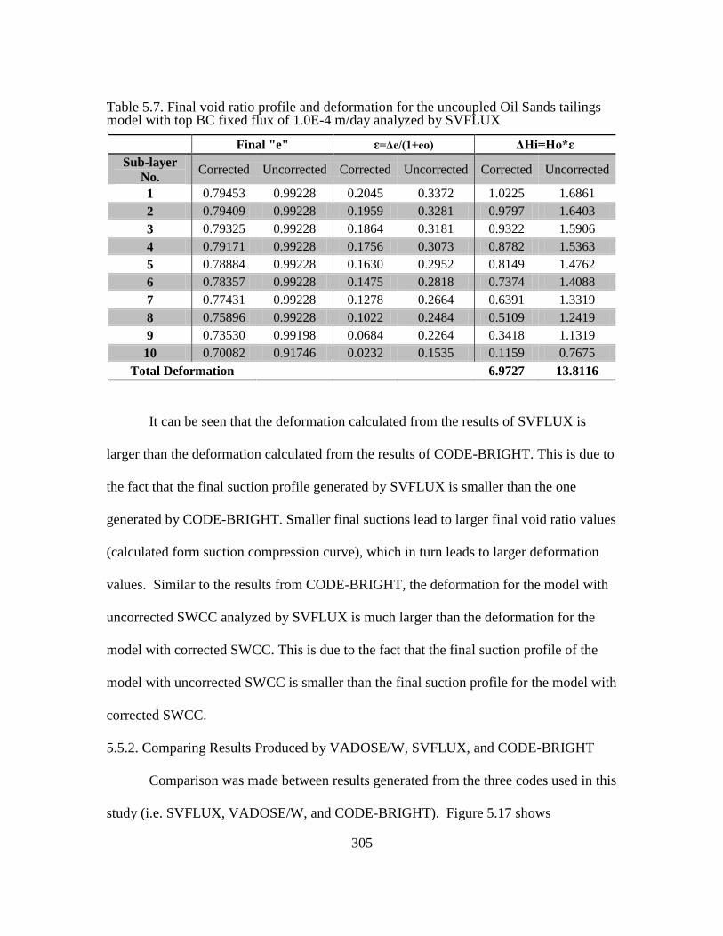
305
Table 5.7. Final void ratio profile and deformation for the uncoupled Oil Sands tailings model with top BC fixed flux of 1.0E-4 m/day analyzed by SVFLUX
Final "e" ε=Δe/(1+eo) ΔHi=Ho*ε
Sub-layer
No. Corrected Uncorrected Corrected Uncorrected Corrected Uncorrected
1 0.79453 0.99228 0.2045 0.3372 1.0225 1.6861
2 0.79409 0.99228 0.1959 0.3281 0.9797 1.6403
3 0.79325 0.99228 0.1864 0.3181 0.9322 1.5906
4 0.79171 0.99228 0.1756 0.3073 0.8782 1.5363
5 0.78884 0.99228 0.1630 0.2952 0.8149 1.4762
6 0.78357 0.99228 0.1475 0.2818 0.7374 1.4088
7 0.77431 0.99228 0.1278 0.2664 0.6391 1.3319
8 0.75896 0.99228 0.1022 0.2484 0.5109 1.2419
9 0.73530 0.99198 0.0684 0.2264 0.3418 1.1319
10 0.70082 0.91746 0.0232 0.1535 0.1159 0.7675
Total Deformation
6.9727 13.8116
It can be seen that the deformation calculated from the results of SVFLUX is
larger than the deformation calculated from the results of CODE-BRIGHT. This is due to
the fact that the final suction profile generated by SVFLUX is smaller than the one
generated by CODE-BRIGHT. Smaller final suctions lead to larger final void ratio values
(calculated form suction compression curve), which in turn leads to larger deformation
values. Similar to the results from CODE-BRIGHT, the deformation for the model with
uncorrected SWCC analyzed by SVFLUX is much larger than the deformation for the
model with corrected SWCC. This is due to the fact that the final suction profile of the
model with uncorrected SWCC is smaller than the final suction profile for the model with
corrected SWCC.
5.5.2. Comparing Results Produced by VADOSE/W, SVFLUX, and CODE-BRIGHT
Comparison was made between results generated from the three codes used in this
study (i.e. SVFLUX, VADOSE/W, and CODE-BRIGHT). Figure 5.17 shows
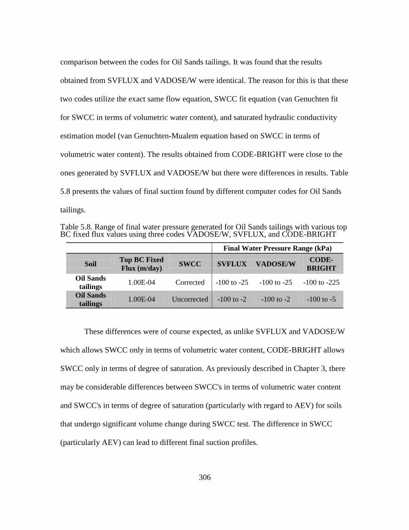
306
comparison between the codes for Oil Sands tailings. It was found that the results
obtained from SVFLUX and VADOSE/W were identical. The reason for this is that these
two codes utilize the exact same flow equation, SWCC fit equation (van Genuchten fit
for SWCC in terms of volumetric water content), and saturated hydraulic conductivity
estimation model (van Genuchten-Mualem equation based on SWCC in terms of
volumetric water content). The results obtained from CODE-BRIGHT were close to the
ones generated by SVFLUX and VADOSE/W but there were differences in results. Table
5.8 presents the values of final suction found by different computer codes for Oil Sands
tailings.
Table 5.8. Range of final water pressure generated for Oil Sands tailings with various top BC fixed flux values using three codes VADOSE/W, SVFLUX, and CODE-BRIGHT
Final Water Pressure Range (kPa)
Soil Top BC Fixed
Flux (m/day) SWCC SVFLUX VADOSE/W
CODE-
BRIGHT
Oil Sands
tailings 1.00E-04 Corrected -100 to -25 -100 to -25 -100 to -225
Oil Sands
tailings 1.00E-04 Uncorrected -100 to -2 -100 to -2 -100 to -5
These differences were of course expected, as unlike SVFLUX and VADOSE/W
which allows SWCC only in terms of volumetric water content, CODE-BRIGHT allows
SWCC only in terms of degree of saturation. As previously described in Chapter 3, there
may be considerable differences between SWCC's in terms of volumetric water content
and SWCC's in terms of degree of saturation (particularly with regard to AEV) for soils
that undergo significant volume change during SWCC test. The difference in SWCC
(particularly AEV) can lead to different final suction profiles.
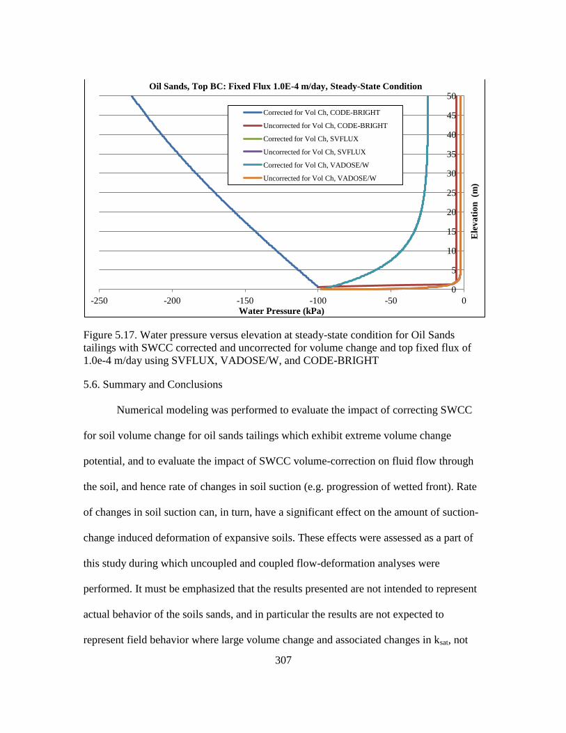
307
Figure 5.17. Water pressure versus elevation at steady-state condition for Oil Sands
tailings with SWCC corrected and uncorrected for volume change and top fixed flux of
1.0e-4 m/day using SVFLUX, VADOSE/W, and CODE-BRIGHT
5.6. Summary and Conclusions
Numerical modeling was performed to evaluate the impact of correcting SWCC
for soil volume change for oil sands tailings which exhibit extreme volume change
potential, and to evaluate the impact of SWCC volume-correction on fluid flow through
the soil, and hence rate of changes in soil suction (e.g. progression of wetted front). Rate
of changes in soil suction can, in turn, have a significant effect on the amount of suction-
change induced deformation of expansive soils. These effects were assessed as a part of
this study during which uncoupled and coupled flow-deformation analyses were
performed. It must be emphasized that the results presented are not intended to represent
actual behavior of the soils sands, and in particular the results are not expected to
represent field behavior where large volume change and associated changes in ksat, not
0
5
10
15
20
25
30
35
40
45
50
-250 -200 -150 -100 -50 0
Ele
va
tio
n (m
)
Water Pressure (kPa)
Oil Sands, Top BC: Fixed Flux 1.0E-4 m/day, Steady-State Condition
Corrected for Vol Ch, CODE-BRIGHT
Uncorrected for Vol Ch, CODE-BRIGHT
Corrected for Vol Ch, SVFLUX
Uncorrected for Vol Ch, SVFLUX
Corrected for Vol Ch, VADOSE/W
Uncorrected for Vol Ch, VADOSE/W
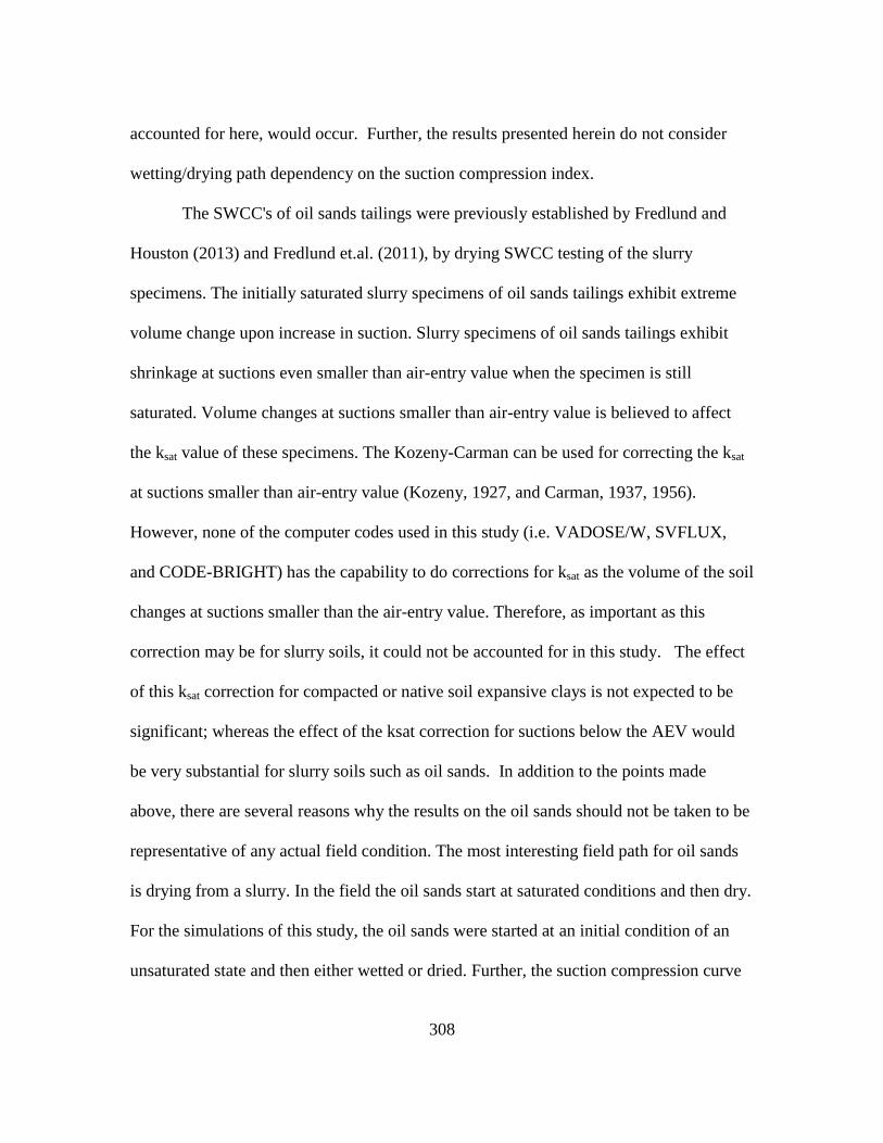
308
accounted for here, would occur. Further, the results presented herein do not consider
wetting/drying path dependency on the suction compression index.
The SWCC's of oil sands tailings were previously established by Fredlund and
Houston (2013) and Fredlund et.al. (2011), by drying SWCC testing of the slurry
specimens. The initially saturated slurry specimens of oil sands tailings exhibit extreme
volume change upon increase in suction. Slurry specimens of oil sands tailings exhibit
shrinkage at suctions even smaller than air-entry value when the specimen is still
saturated. Volume changes at suctions smaller than air-entry value is believed to affect
the ksat value of these specimens. The Kozeny-Carman can be used for correcting the ksat
at suctions smaller than air-entry value (Kozeny, 1927, and Carman, 1937, 1956).
However, none of the computer codes used in this study (i.e. VADOSE/W, SVFLUX,
and CODE-BRIGHT) has the capability to do corrections for ksat as the volume of the soil
changes at suctions smaller than the air-entry value. Therefore, as important as this
correction may be for slurry soils, it could not be accounted for in this study. The effect
of this ksat correction for compacted or native soil expansive clays is not expected to be
significant; whereas the effect of the ksat correction for suctions below the AEV would
be very substantial for slurry soils such as oil sands. In addition to the points made
above, there are several reasons why the results on the oil sands should not be taken to be
representative of any actual field condition. The most interesting field path for oil sands
is drying from a slurry. In the field the oil sands start at saturated conditions and then dry.
For the simulations of this study, the oil sands were started at an initial condition of an
unsaturated state and then either wetted or dried. Further, the suction compression curve

309
(void ratio versus suction) of oil sands tailings obtained from previous research by
Fredlund et al. (2011) was utilized, and in those studies a drying path was followed. For
the cases in which a wetting path was simulated in the numerical analyses for the oil
sands tailings, no modification to the void ratio versus suction relationship to account for
difference in wetting and drying path were made in this study.
Uncoupled (flow only) analyses were conducted for the models based on
properties of oil sands tailings in SVFLUX, VADOSE/W, and CODE-BRIGHT in order
to evaluate effect of volume-correcting SWCC on hydraulic properties of soils and
changes in soil suction (e.g. progression of wetted front) and hence soil volume change
due to wetting. The rate of changes in soil suction was studied and amount of suction-
change induced deformation was determined based on the generated suction profile of the
soil column. For this purpose, the suction compression curve (void ratio versus suction)
of oil sands tailings obtained from previous research by Fredlund and Houston (2013),
and Fredlund et al. (2011) was utilized.
Initial condition of the soil unsaturated (suction of 100kPa at the bottom and
suction of 600kPa at the top of the model). For the simulations in which the soil becomes
wet from the top by adding the positive fixed flux, the suction of soil starts to decrease. In
other words, the wetting path on the SWCC is followed. It was previously established
that the volume corrected SWCC generally has larger AEV compared to the uncorrected
SWCC. This means that in the soil with volume corrected SWCC, desaturation starts at a
larger suction compared to the soil with uncorrected SWCC. That is to say, the soil with
corrected SWCC stays saturated at larger suction ranges compared to the soil with

310
uncorrected SWCC. Therefore, once the soil becomes wet and the suction decreases (i.e.
wetting path on the SWCC), for the soil with corrected SWCC, the soil becomes
saturated (i.e. close to AEV on SWCC) at a larger suction. Whereas, the suction within
the soil with uncorrected SWCC should further decrease (compared to the soil with
corrected SWCC) in order for the suction to reach AEV (i.e. saturation or close-to-
saturation state). This mechanism illustrates the reason for the difference in final suction
profile for the cases of volume corrected SWCC and volume uncorrected SWCC. It
should be mentioned that for a certain expansive soil, the smaller final suction within the
soil profile indicates larger values of deformation. This is due to the general shape of
suction compression curves, in which the void ratio of the expansive soils is larger at
smaller suction values (i.e. when the soil is wetter).
An example of generated suction profile for oil sands tailings with base BC set as
suction of 100kPa is shown in Figure 5.18. It can be seen that if the model is allowed to
run for long-enough time so that the soil gets fully wetted (i.e. steady-state); the
generated suction is smaller for uncorrected SWCC compared to corrected SWCC. This
is due to the fact that the volume-corrected SWCC has a larger air-entry value compared
to volume-uncorrected SWCC. Therefore, when the soil becomes wet (i.e. wetting path
on SWCC) the volume-corrected SWCC reaches the saturated condition at a higher
suction.
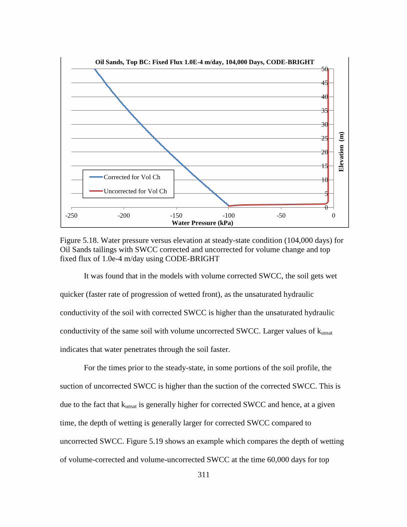
311
Figure 5.18. Water pressure versus elevation at steady-state condition (104,000 days) for
Oil Sands tailings with SWCC corrected and uncorrected for volume change and top
fixed flux of 1.0e-4 m/day using CODE-BRIGHT
It was found that in the models with volume corrected SWCC, the soil gets wet
quicker (faster rate of progression of wetted front), as the unsaturated hydraulic
conductivity of the soil with corrected SWCC is higher than the unsaturated hydraulic
conductivity of the same soil with volume uncorrected SWCC. Larger values of kunsat
indicates that water penetrates through the soil faster.
For the times prior to the steady-state, in some portions of the soil profile, the
suction of uncorrected SWCC is higher than the suction of the corrected SWCC. This is
due to the fact that kunsat is generally higher for corrected SWCC and hence, at a given
time, the depth of wetting is generally larger for corrected SWCC compared to
uncorrected SWCC. Figure 5.19 shows an example which compares the depth of wetting
of volume-corrected and volume-uncorrected SWCC at the time 60,000 days for top
0
5
10
15
20
25
30
35
40
45
50
-250 -200 -150 -100 -50 0
Ele
va
tio
n (m
)
Water Pressure (kPa)
Oil Sands, Top BC: Fixed Flux 1.0E-4 m/day, 104,000 Days, CODE-BRIGHT
Corrected for Vol Ch
Uncorrected for Vol Ch
312
boundary condition of fixed flux of 1.0E-4 m/day for oil sands tailings. It can be seen that
the depth of wetting is larger for corrected SWCC (due to higher kunsat values). Figure
5.19shows that at time 60,000 days the model with the volume-corrected SWCC has
reached the steady-state (fully wetted condition) while the model with the volume-
corrected SWCC is only wetted half-way through the depth of column.
Figure 5.19. Water pressure versus elevation at time 60,000 days (164 years) for Oil
Sands tailings with SWCC corrected and uncorrected for volume change and top fixed
flux of 1.0e-4 m/day using CODE-BRIGHT
Figure 5.20 shows an example for top boundary condition of evaporation for oil
sands tailings. It was found that for top boundary conditions of negative flux
(evaporation) the generated suction was larger for volume-uncorrected SWCC compared
to volume-corrected SWCC. This makes it difficult to determine in advance if corrected
or uncorrected curves will lead to higher suction values, particularly for evaporation
0
5
10
15
20
25
30
35
40
45
50
-350 -300 -250 -200 -150 -100 -50 0
Ele
va
tio
n (
m)
Water Pressure (kPa)
Oil Sands, Top BC: Fixed Flux 1.0E-4 m/day, 60,000 Days, CODE-BRIGHT
Corrected for Vol Ch
Uncorrected for Vol Ch
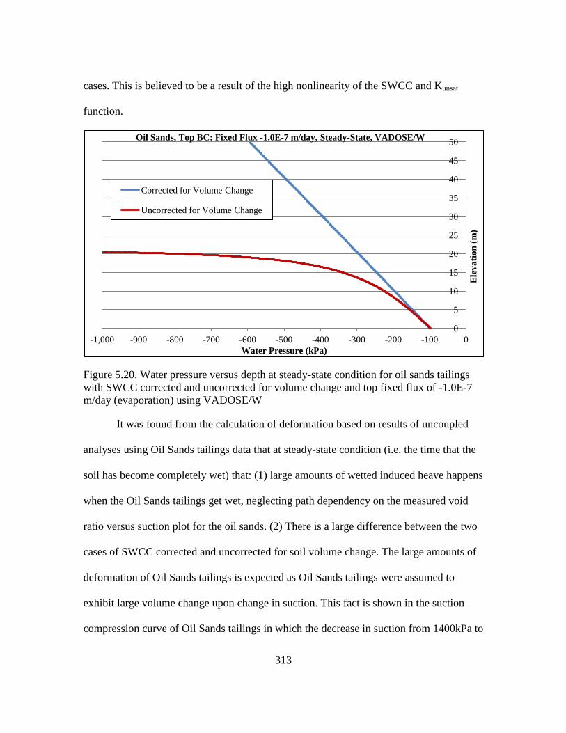
313
cases. This is believed to be a result of the high nonlinearity of the SWCC and Kunsat
function.
Figure 5.20. Water pressure versus depth at steady-state condition for oil sands tailings
with SWCC corrected and uncorrected for volume change and top fixed flux of -1.0E-7
m/day (evaporation) using VADOSE/W
It was found from the calculation of deformation based on results of uncoupled
analyses using Oil Sands tailings data that at steady-state condition (i.e. the time that the
soil has become completely wet) that: (1) large amounts of wetted induced heave happens
when the Oil Sands tailings get wet, neglecting path dependency on the measured void
ratio versus suction plot for the oil sands. (2) There is a large difference between the two
cases of SWCC corrected and uncorrected for soil volume change. The large amounts of
deformation of Oil Sands tailings is expected as Oil Sands tailings were assumed to
exhibit large volume change upon change in suction. This fact is shown in the suction
compression curve of Oil Sands tailings in which the decrease in suction from 1400kPa to
0
5
10
15
20
25
30
35
40
45
50
-1,000 -900 -800 -700 -600 -500 -400 -300 -200 -100 0
Ele
va
tio
n (
m)
Water Pressure (kPa)
Oil Sands, Top BC: Fixed Flux -1.0E-7 m/day, Steady-State, VADOSE/W
Corrected for Volume Change
Uncorrected for Volume Change

314
60kPa leads to increase in void ratio from around 0.35 to 0.72 (i.e. increase of 0.37 in
void ratio) when it is assumed that the wetting and drying path void ratio versus suction
curves are the same. This large amount of increase in void ratio leads to large amounts of
strain and thus heave. The final suction profile of the case in which SWCC is uncorrected
is much smaller than the suction within the Oil Sands tailings in case of corrected SWCC.
By using the same suction compression curve, much larger final void ratio profile for the
case with uncorrected SWCC is found compared to the case in which SWCC is corrected.
Larger final void ratio throughout the soil column leads to more deformation of the model
with uncorrected SWCC (2.6m and 11.8m for corrected and uncorrected SWCC,
respectively found by uncoupled analyses using CODE-BRIGHT).
It was also found that depending upon the time and amount of progression of
wetted front within the profile, uncorrected SWCC may exhibit higher or lower suction
compared to the corrected SWCC. This makes it difficult to determine in advance if
corrected or uncorrected curves will lead to higher suction values, and further research is
needed to study this phenomenon from a fundamental unsaturated soil mechanics
perspective.
315
Chapter 6
SUMMARY, CONCLUSIONS AND RECOMMENDATIONS FOR FUTURE
RESEARCH
6.1. Summary
The SWCC can be used to estimate unsaturated soil properties such as unsaturated
hydraulic conductivity. Therefore, the accuracy of the unsaturated soil property depends
on the accuracy of the SWCC. Several factors such as soil structure, initial water content,
void ratio, and compaction method can have significant effects on the SWCC, suggesting
that matching the laboratory conditions for SWCC determination to field conditions may
be most appropriate. Even though the soil water characteristic curve has been measured
and used by numerous researchers throughout the years, the effect of volume change for
high volume change soils (e.g. expansive soils) has rarely been considered when
determining the SWCC's. Failure to consider volume change leads to inaccurate SWCC's
including errors in the air-entry value and the slope in the transition zone, and the errors
are most pronounced for soils that exhibit high volume change in response to changes in
soil suction. Furthermore, it has been the common practice to estimate some of the major
unsaturated soil property functions (e.g., unsaturated hydraulic conductivity function and
unsaturated soil shear strength) by using the saturated soil properties together with the
SWCC, which gives further support for recognizing the importance of establishing
accurate SWCC for high volume change soils. In recent years, the importance of
considering the volume change of soils during suction change has been recognized by a
number of researchers, including Salager et al. (2010), Pe´ron et al. (2007), Nuth and
316
Laloui (2011), Stange and Horn (2005), Mbonimpa et al. (2006), Fredlund et al. (2011),
and Fredlund and Houston, (2013).
Through literature study it was found that the effect of net normal stress which is
applied to the soil specimen during the SWCC testing has also been under-studied,
particularly the effect of net normal stress on suction-changed induced soil volume
change. Only very few researchers have conducted studies for evaluating the impact of
net normal stress on volume change of expansive soils and its impact on shape of the
SWCC. Furthermore, the effect of the initial state of the soil specimen, including initial
moisture content and structure, on the SWCC has not been studied extensively. It is
known that the initial condition of the soil (slurry versus compacted) can have a
significant effect on the SWCC of the soil, particularly with regard to soil volume change
(Fredlund, 2002), yet SWCC's used in practice are often determined for conditions of the
soils that do not match those anticipated in the field prototype.
Correction of SWCC's for soil volume change has been shown to have a
considerable impact on air-entry value and shape of the SWCC (including the slope in the
transition zone). This, in turn, has a significant impact on unsaturated soil properties
derived from the SWCC's (e.g. unsaturated hydraulic conductivity function). No studies
could be found in that literature using numerical modeling to demonstrate the effect of
correction of SWCC for soil volume change on hydraulic properties of the soils (e.g.
advancement of wetted front) and its impact on the amount of suction-change induced
deformation of expansive soils.
317
An extensive literature review was conducted on the methods of SWCC
determination and the models available to best-fit the SWCC data obtained from
laboratory experiments. It was found that, although not always mentioned, the underlying
assumption of SWCC fitting equations is that the soil is sufficiently stiff so that there is
no change in pore size distribution during the test (Mbonimpa et al., 2006, Chiu and Ng,
2012.
It was found through literature search that researchers have measured soil volume
change for determination of SWCC(Stange and Horn (2005), Cui et al. (2006) , Chao et
al. (2008), Perez-Garcia, et al. (2008), Salager et al. (2010), Vazquez and Durand (2011),
Qi and Michel (2011), Chiu and Ng (2012), Ng et al. (2012), Liu et al. (2012, 2011)). It
was also found that some researchers who studied the effect of volume change on
SWCC's have recommended using degree of saturation SWCC as opposed to gravimetric
or volumetric moisture content SWCC's (Li et al., 2007, Parent et al., 2007, Nuth and
Laloui, 2008, Chiu and Ng, 2012, Fredlund and Houston, 2013).
Use of soil water characteristic curves in constitutive relations for unsaturated
soils, in particular unsaturated hydraulic conductivity functions, was also studied through
a literature search. Commonly used equations to estimate unsaturated hydraulic
conductivity functions of soils based on the SWCC were studied. This part of the
literature search included studying the methodologies and database used for developing
the equations for estimating unsaturated hydraulic conductivity functions as well as the
applications of the proposed equations. It was found that the most common equations
used for estimating unsaturated hydraulic conductivity functions of soils were developed
318
for silts and sands, that is using a database developed primarily on silts and sands.
Undisturbed and compacted specimens of silts and sands were typically used for
developing or validating these equations. Volume change of soils was not considered
when developing these equations for estimation of unsaturated hydraulic conductivity,
and the equations were found to work best for silts and sands. There appears to be a need
for improvement to estimation of unsaturated hydraulic conductivity functions for high
volume change soils, including expansive clays, and a larger database for development of
improved unsaturated hydraulic conductivity estimation methods is needed, particularly
for fine-grained soils.
The importance of correcting SWCC's (including SWCC's in terms of volumetric
water content and degree of saturation) for soil volume change was studied through
literature search. Additional literature search was carried out to assess the effect of net
normal stress on the shape of SWCC with regard to the soil volume change throughout
the test. Moreover, the importance of the initial condition of the specimen (slurry versus
compacted specimen) was evaluated through literature search. The literature review
showed that slurry specimens undergo significant volume change during SWCC test.
Therefore, for a certain clay soils the SWCC of the slurry specimen may be significantly
different from that of the compacted specimen.
The hysteresis loop present between the wetting and drying paths of a SWCC was
also studied through literature search. Numerous researchers have measured SWCC's
including drying and wetting paths and presented the hysteresis associated with the
curves. It is well known that at a given soil suction, the water content of the drying curve
319
is higher than that of the wetting curve (i.e. the drying curve lies above the wetting
curve). Furthermore, the end point of the wetting curve differs from the starting point of
the drying curve because of air entrapment in the soil that occurs upon drying.
Furthermore, the slope of the drying curve is approximately parallel to that of the wetting
curve.
The impact of net normal stress applied to the specimen during the SWCC test
was studied through literature search. Very limited data was found regarding the effect of
net normal stress on the shape of the SWCC's. It was found that in general, the applied
normal stress does not seem to affect the shape of the SWCC significantly; however, the
AEV increases and the rate of degree of saturation change decreases with increasing the
net normal stress (Ng and Pang 2000 and Vanapalli et al. 1999).
As the next part of study, soil water characteristic curves (SWCC) of three
expansive clays, Anthem, Colorado, and San Antonio, were determined through
laboratory tests. The first set of tests was conducted on compacted specimens under net
normal stress of 7kPa (seating load). The purpose of this set of test was to evaluate effect
of considering soil volume change on the shape of SWCC of expansive clays, with
particular focus on the air-entry value. Another set of tests were conducted in which
slurry specimens of the soils were tested. The slurry specimens were prepared by mixing
certain amount of soil and water to make sure that the specimen had reached 100%
saturation. The effect of initial state of the specimen on its SWCC was studied by this set
of experiments. It was found that slurry specimens undergo significant volume changes
during SWCC testing as soil suction is changed. Therefore, the difference between the
320
volume corrected SWCC and uncorrected SWCC was more significant for slurry
specimens compared to compacted specimens.
The last set of laboratory experiments were intended to help evaluate the effect of
net normal stress on the volume change of specimens and its impact on the shape of
SWCC. For this set of experiments, different net normal stresses were used. The range of
net normal stresses was from 7kPa to around 55% of the swell pressure of the tested soil.
Volume corrected SWCC's were developed by using the instantaneous volume of the
specimen while in volume uncorrected SWCC's the initial volume of the specimen was
used as the reference and the soil volume change throughout the test was ignored.
The next part of the study included numerical modeling that was performed to
find the impact of correcting SWCC for soil volume change (for soils with high volume
change potential) and to evaluate the impact of SWCC correction on fluid flow through
the soil, and hence rate and degree of change of suction within the soil profile. Rate of
changes in soil suction can, in turn, have a significant effect on the amount of
deformation of expansive soils. The effects of volume change correction on the SWCC
and the associated estimation of the kunsat function on suction-change induced
deformations were assessed as a part of this study using uncoupled and coupled flow-
deformation analyses. For uncoupled analyses, the unsaturated flow only is evaluated and
then the results from the flow analysis (i.e., initial and final soil suction profiles) are used
as input to a separate deformation analysis. For a coupled flow-deformation analysis,
however, unsaturated flow and suction-change induced deformation are solved for at the
same time, considering any effect of suction change on deformation and any effect of
321
deformation on soil suction, by solving the governing partial differential equations for
flow and stress-deformation simultaneously.
Three computer programs of VADOSE/W, CODE-BRIGHT, and SVFLUX were
used to evaluate the effect of volume-correcting SWCC's on fluid flow through the soils
and the resulting suction-change induced deformation. These computer codes have the
capability of simulating saturated and unsaturated flow of water through soils and are
commonly used in industry and/or academia (research projects).
The laboratory results obtained from SWCC tests on the three expansive soils of
Anthem, Colorado, and San Antonio as well as data obtained from previous research
conducted on oil sands tailings by Fredlund and Houston (2013) and Fredlund et.al.
(2011) were used in the numerical modeling. One-dimensional flow through a soil was
simulated to study the flow through a column of soil once with the SWCC corrected and
once with the SWCC uncorrected for volume change.
Uncoupled (flow only) analyses were conducted for the models in SVFLUX,
VADOSE/W, and CODE-BRIGHT in order to evaluate impact of correcting the SWCC
for volume change on hydraulic properties of soils and the rate of change of soil suction
in the profile, and hence soil volume change due to wetting or drying. For positive flux
surface boundary conditions, the rate of progression of wetted front was studied and the
amount of soil expansion (heave) was determined based on the initial and final suction
profile of the soil column. For this purpose, the suction compression curves (void ratio
versus log of suction) of specimens obtained from SWCC laboratory experiments on the
322
expansive clays were utilized as well as the suction compression curves obtained from
previous research conducted on oil sands tailings by Fredlund et.al. (2011).
6.2. Conclusions
During the literature review, particular focus was placed upon studying whether in
common practice SWCC's are corrected for soil volume change. This was studied
particularly for the soils with high volume change potential. Soil water characteristic
curve fitting equations have been generated by a number of researchers (e.g., Gardner
1956; Brooks and Corey 1964; van Genuchten 1980; Fredlund and Xing 1994). Although
not always mentioned, the underlying assumption of most SWCC fitting equations is that
the soil is sufficiently stiff so that there is no change in void ratio of the soil (i.e. no soil
volume change) during the test (Mbonimpa et al., 2006, Chiu and Ng, 2012). It was found
that in recent years a number of researchers have recognized the importance of
considering soil volume change when establishing SWCC's. Some researchers have
conducted SWCC tests during which the volume and mass of the specimen has been
recorded and the volume change of the specimen has been incorporated when generating
the SWCC's (Stange and Horn 2005, Cui et al. 2006, Chao et al. 2008, Salager et al.
2010, Vazquez and Durand 2011, Qi and Michel 2011, Chiu and Ng 2012, Ng et al. 2012,
Liu et al. 2012, 2011, Perez-Garcia, et al. 2008). At the same time, the measured data
comparing volume change corrected and uncorrected SWCC's was very limited and the
researchers reported either the SWCC that is corrected for volume change or the SWCC
uncorrected for volume change. It was found through literature study that only very few
researchers have compared SWCC's with and without volume change consideration to
assess the impact on key SWCC parameters such as AEV and slope in transition zone.
323
A number of researchers recommended using degree of saturation SWCC as
opposed to gravimetric moisture content. The authors reported that when the soil
undergoes volume change during a suction increase, only the degree of saturation
variable clearly defines the air-entry value for the soil (as opposed to gravimetric and
volumetric water content).
No researchers were found to have evaluated the effect of initial state of
expansive soils specimens (i.e. slurry versus compacted specimens) on SWCC with focus
on volume change. Very few studies on effect of net normal stress on soil volume change
and its impact on SWCC of expansive clays was found in the literature.
Three of the most commonly used equations for estimating the unsaturated
hydraulic conductivity function of soils were studied through literature search. The
purpose of this part of the literature review was to study the basis upon which these
unsaturated hydraulic conductivity fitting equations have been developed and validated,
and also to find the database and applications for each model (i.e. is the model applied
best for coarse or fine-grained materials). The description of three common unsaturated
hydraulic conductivity estimation models includes the methods which the researchers
utilized for developing the models as well as the validation of the models by comparing
the estimated values against measured values of unsaturated hydraulic conductivity. The
three models that are described are the model by Green and Corey (1971), Fredlund et al.
(2004), and van Genuchten (1980). It was found that the underlying assumption for
generating these equations, in all cases, is that the volume change of the soil structure is
negligible. It was found that the most common equations used for estimating unsaturated

324
hydraulic conductivity functions of soils were developed using data on silts and sands.
Undisturbed and compacted specimens of silts and sands were used for developing or
validating these equations. Volume change of soils was not considered when developing
these equations for estimating unsaturated hydraulic conductivity and these equations are
expected to work best for silts and sands but may not accurately estimate unsaturated
hydraulic conductivity functions of clays or for any soils that exhibit significant volume
change as soil suction changes under a given net normal stress condition.
No studies were found on the effect of volume change consideration on the
hydraulic properties of the soils together with associated unsaturated flow modeling (e.g.
advancement of wetted front). No researchers were found to have focused on the effect of
volume change on the SWCC as related to unsaturated flow/deformation analyses for
expansive clays.
As a main scope of this research, the SWCC's of three expansive soils were
measured through laboratory testing using an oedometer pressure plate device for suction
up to 1500 kPa ) and the filter paper method for higher suctions. Volume change of the
soils during suction change was measured and taken into account for establishing the
SWCC's in terms of volumetric water content and degree of saturation. The measured
data points along with the van Genuchten (1980) SWCC fitting parameters were
presented.
Volume corrected SWCC's were developed by using the instantaneous volume of
the specimen while volume uncorrected SWCC's were developed using initial volume of
the specimen (i.e. volume changes throughout the test was ignored).
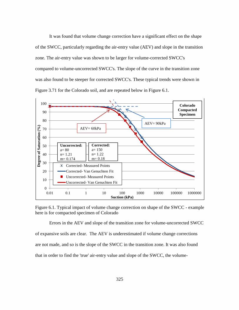
325
It was found that volume change correction have a significant effect on the shape
of the SWCC, particularly regarding the air-entry value (AEV) and slope in the transition
zone. The air-entry value was shown to be larger for volume-corrected SWCC's
compared to volume-uncorrected SWCC's. The slope of the curve in the transition zone
was also found to be steeper for corrected SWCC's. These typical trends were shown in
Figure 3.71 for the Colorado soil, and are repeated below in Figure 6.1.
Figure 6.1. Typical impact of volume change correction on shape of the SWCC - example
here is for compacted specimen of Colorado
Errors in the AEV and slope of the transition zone for volume-uncorrected SWCC
of expansive soils are clear. The AEV is underestimated if volume change corrections
are not made, and so is the slope of the SWCC in the transition zone. It was also found
that in order to find the 'true' air-entry value and slope of the SWCC, the volume-
0
10
20
30
40
50
60
70
80
90
100
0.01 0.1 1 10 100 1000 10000 100000 1000000
Deg
ree
of
Sa
tura
tio
n (
%)
Suction (kPa)
Corrected- Measured Points
Corrected- Van Genuchten Fit
Uncorrected- Measured Points
Uncorrected- Van Genuchten Fit
Corrected:
a= 150
n= 1.22
m= 0.18
Uncorrected:
a= 80
n= 1.21
m= 0.174
AEV= 90kPa
AEV= 60kPa
Colorado
Compacted
Specimen
326
corrected SWCC in terms of degree of saturation, which givens the highest AEV, should
be used, as previously discussed by Fredlund and Houston (2013).
Another major finding from the SWCC lab testing program is that due to the
existence of clods in soils with high plasticity during the compaction process, the air-
entry value of these soils turns out to be lower than what is normally expected for high
plasticity soils. The relatively low air-entry values observed are believed to be the result
of existence of clods creating air-entry values more consistent with coarser-grained
materials. In order to evaluate the effects of clods on the SWCC of the three clays of this
study, with particular focus on the air-entry value, SWCC tests were performed on slurry
specimens. In slurry specimens, the pulverized soil was entirely saturated with water and
therefore clods did not appear within the specimen. Slurry specimens of Anthem,
Colorado, and San Antonio soils were tested and the resulting SWCC's were compared
against the SWCC's obtained from the compacted specimens of the same soils. It was
found that the initial state of the specimen has a significant effect on the shape of the
SWCC, as a result of both structure and volume change. In particular, the shape of the
SWCC including volume corrections was dramatically affected on the slurry specimens
due to high volume change experienced by the slurry specimens as suction changes were
imposed. For any given soil tested, the air-entry value of volume-corrected SWCC's
obtained from testing slurry specimens was found to be higher than that of compacted
specimens. The slope in transition zone was also found to be higher for slurry specimens.
It was found that slurry specimens showed generally larger AEV compared to compacted
specimens due to a combination of volume change and structure effects. Figure 6.2,
327
shows the SWCC in terms of degree of saturation including both corrected and
uncorrected curves for slurry specimen of San Antonio soil. Also shown is the volume-
corrected SWCC for compacted specimen of San Antonio soil. The figure shows the
significant difference in AEV and slope in the transition zone between corrected and
uncorrected curves for the slurry specimen. Furthermore, the differences discussed above
between slurried and compacted soil specimen SWCC's are obvious in Figure 6.2. It
should be mentioned that the net normal stress in both cases (slurry and compacted
specimens tested) was a token load, but some differences could be due to slurry
specimens having 3kPa token load while the compacted specimen had 7kPa token load.
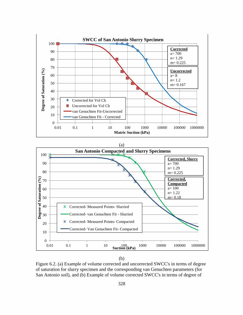
328
(a)
(b)
Figure 6.2. (a) Example of volume corrected and uncorrected SWCC's in terms of degree
of saturation for slurry specimen and the corresponding van Genuchten parameters (for
San Antonio soil), and (b) Example of volume corrected SWCC's in terms of degree of
0
10
20
30
40
50
60
70
80
90
100
0.01 0.1 1 10 100 1000 10000 100000 1000000
Deg
ree
of
Sa
tura
tio
n (
%)
Matric Suction (kPa)
SWCC of San Antonio Slurry Specimen
Corrected for Vol Ch
Uncorrected for Vol Ch
van Genuchten Fit-Uncorrected
van Genuchten Fit - Corrected
Uncorrected
a= 8
n= 1.2
m= 0.167
Corrected
a= 700
n= 1.29
m= 0.225
0
10
20
30
40
50
60
70
80
90
100
0.01 0.1 1 10 100 1000 10000 100000 1000000
Deg
ree
of
Sa
tura
tio
n (
%)
Suction (kPa)
San Antonio Compacted and Slurry Specimens
Corrected- Measured Points- Slurried
Corrected- van Genuchten Fit - Slurried
Corrected- Measured Points- Compacted
Corrected- Van Genuchten Fit- Compacted
Corrected,
Compacted
a= 100
n= 1.22
m= 0.18
Corrected, Slurry
a= 700
n= 1.29
m= 0.225
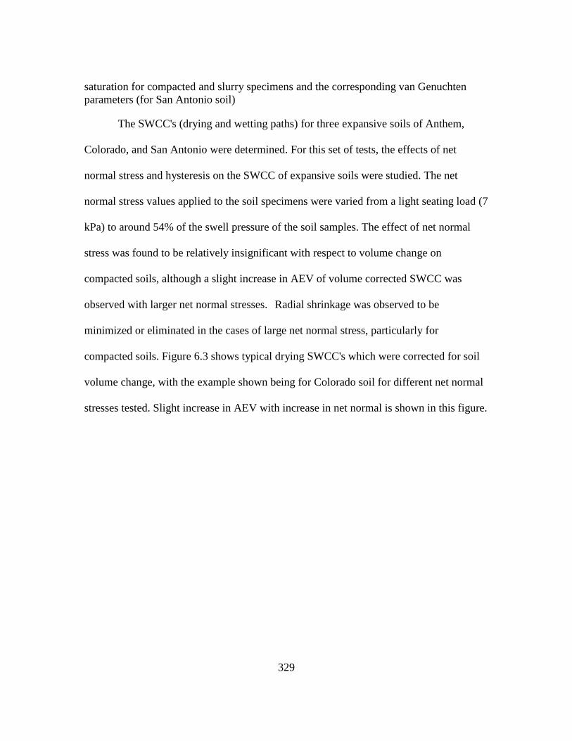
329
saturation for compacted and slurry specimens and the corresponding van Genuchten
parameters (for San Antonio soil)
The SWCC's (drying and wetting paths) for three expansive soils of Anthem,
Colorado, and San Antonio were determined. For this set of tests, the effects of net
normal stress and hysteresis on the SWCC of expansive soils were studied. The net
normal stress values applied to the soil specimens were varied from a light seating load (7
kPa) to around 54% of the swell pressure of the soil samples. The effect of net normal
stress was found to be relatively insignificant with respect to volume change on
compacted soils, although a slight increase in AEV of volume corrected SWCC was
observed with larger net normal stresses. Radial shrinkage was observed to be
minimized or eliminated in the cases of large net normal stress, particularly for
compacted soils. Figure 6.3 shows typical drying SWCC's which were corrected for soil
volume change, with the example shown being for Colorado soil for different net normal
stresses tested. Slight increase in AEV with increase in net normal is shown in this figure.
330
Figure 6.3. Typical effect of net normal stress on compacted expansive soils SWCC’s –
shown here are Drying SWCC's for Colorado soil (swell pressure: 250 kPa) under various
net normal stresses. Notice larger values of "a" parameter for tests under higher net
normal stress
As illustrated in the images of the specimens shown in Chapter 3, generally larger
radial shrinkage was observed at larger suctions (e.g. around 1300 kPa) compared to at
lower suctions (e.g. 200 kPa). It was found that with increase in suction, the radial
shrinkage of the soil specimens also increase, as expected. This was true for the cases of
both slurry and compacted specimens, although the compacted specimens generally
exhibit relatively small radial shrinkage during drying curve SWCC determination, even
under low confining stress. When comparing the shrinkage of compacted specimens it
was found that with increase in net normal stress, the amount of radial shrinkage of the
soil decreases. It was found that for the compacted specimens which were tested under
large amounts of net normal stress (e.g. around 50% of the swell pressure of the soil) the
0
10
20
30
40
50
60
70
80
90
100
0.01 0.1 1 10 100 1000 10000 100000 1000000
Deg
ree
of
Sa
tura
tio
n (
%)
Matric Suction (kPa)
Drying SWCC of Colorado Compacted Specimens
7kPa, Seating Load
21% Swell Pressure
42% Swell Pressure
van Genuchten fit - 7 kPa
van Genuchten fit - 21% SP
van Genuchten fit - 42% SP
7 kPa
a= 170
n= 1.25
m= 0.200
105kPa (42
% SP)
a= 200
n= 1.24
m= 0.194
53kPa (21
% SP)
a= 190
n=1.22
m=0.18
331
radial shrinkage of the soil during the drying SWCC test was minimal such that the
contact between the soil and the confining ring was maintained throughout the test even
at relatively large suction values (i.e. around 1300 kPa). For such cases in which the
contact between the soil and the confining ring is maintained throughout the test, the
volume change of the soil is only in the vertical direction. This volume change can be
measured much easier and with more accuracy compared to cases where the specimen
shrinks away from the specimen ring. Of course, when the path is wetting rather than
drying, there is no shrinkage issue to deal with in determining the SWCC. Given that the
wetting path is commonly the path of interest in the field, it could be argued that further
study on the impact/improvement for using the wetting path in determining the SWCC is
needed.
The laboratory results obtained from the SWCC tests on the three soils of
Anthem, Colorado, and San Antonio were used in the unsaturated flow/deformation
numerical modeling studies. One-dimensional unsaturated flow through a soil was
simulated to study the flow through a column of soil once with the SWCC corrected and
once with the SWCC uncorrected for volume change.
Uncoupled (flow only) analyses were conducted for the models in SVFLUX,
VADOSE/W, and CODE-BRIGHT in order to evaluate impact of correcting SWCC for
volume change on hydraulic properties of soils and the rate of change and magnitude of
change of soil suction in the profile, and hence soil volume change due to wetting or
drying. For positive flux surface boundary conditions, rate of progression of wetted front
was studied and amount of soil expansion (heave) was determined based on the initial

332
and final suction profile of the soil column. For this purpose, the suction compression
curves (void ratio versus log of suction) of specimens obtained from SWCC laboratory
experiments on the expansive clays were utilized.
In this study, the initial condition of the modeled soil was set as unsaturated. For
the cases in which the soil becomes wetted from the top by adding a positive fixed flux to
the top of the soil column, the suction of soil starts to decrease. In other words, the
wetting path on the SWCC is followed when the soil becomes wetted. It was previously
established that the volume corrected SWCC generally has larger AEV compared to the
uncorrected SWCC. This means that in the soil with volume corrected SWCC,
desaturation starts at a larger suction compared to the soil with uncorrected SWCC. That
is to say, the soil with corrected SWCC stays saturated at larger suction ranges compared
to the soil with uncorrected SWCC. Therefore, once the soil becomes wet and the suction
decreases (i.e. wetting path on the SWCC), for the soil with corrected SWCC, the soil
becomes saturated (i.e. close to AEV on SWCC) at a larger suction; whereas, the suction
within the soil with uncorrected SWCC must decrease further (compared to the soil with
corrected SWCC) in order for the suction to reach the AEV (i.e. saturation or close-to-
saturation state). This mechanism illustrates the reason for the difference in final suction
values for the cases of volume corrected SWCC and volume uncorrected SWCC when
the soil becomes wetted. It should be mentioned that for a certain expansive soil and
given initial head (suction) boundary conditions, the smaller final suction within the soil
profile leads to larger values of deformation. An example of generated suction profile for
Colorado soil with base boundary condition set as suction of 100kPa is shown in Figure
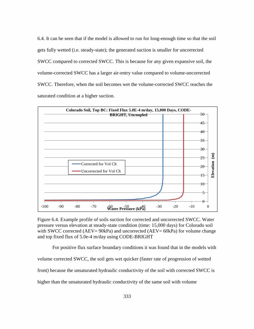
333
6.4. It can be seen that if the model is allowed to run for long-enough time so that the soil
gets fully wetted (i.e. steady-state); the generated suction is smaller for uncorrected
SWCC compared to corrected SWCC. This is because for any given expansive soil, the
volume-corrected SWCC has a larger air-entry value compared to volume-uncorrected
SWCC. Therefore, when the soil becomes wet the volume-corrected SWCC reaches the
saturated condition at a higher suction.
Figure 6.4. Example profile of soils suction for corrected and uncorrected SWCC. Water
pressure versus elevation at steady-state condition (time: 15,000 days) for Colorado soil
with SWCC corrected (AEV= 90kPa) and uncorrected (AEV= 60kPa) for volume change
and top fixed flux of 5.0e-4 m/day using CODE-BRIGHT
For positive flux surface boundary conditions it was found that in the models with
volume corrected SWCC, the soil gets wet quicker (faster rate of progression of wetted
front) because the unsaturated hydraulic conductivity of the soil with corrected SWCC is
higher than the unsaturated hydraulic conductivity of the same soil with volume
0
5
10
15
20
25
30
35
40
45
50
-100 -90 -80 -70 -60 -50 -40 -30 -20 -10 0
Ele
va
tio
n (m
) Water Pressure (kPa)
Colorado Soil, Top BC: Fixed Flux 5.0E-4 m/day, 15,000 Days, CODE-
BRIGHT, Uncoupled
Corrected for Vol Ch
Uncorrected for Vol Ch
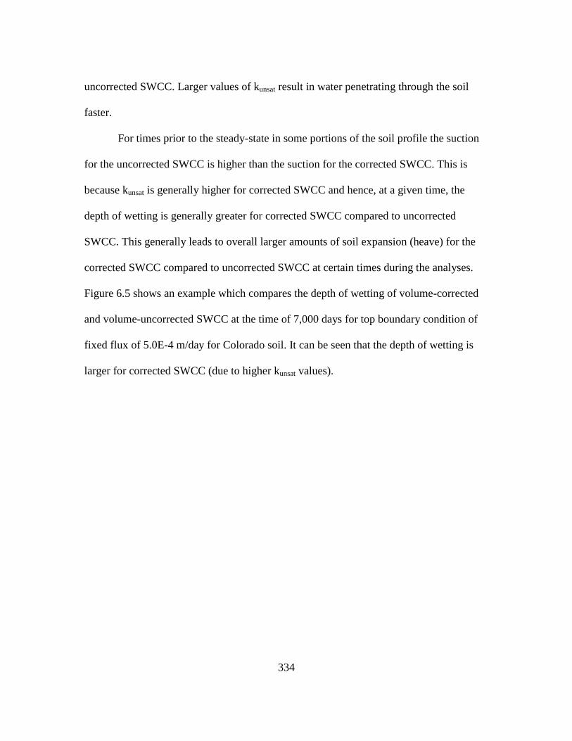
334
uncorrected SWCC. Larger values of kunsat result in water penetrating through the soil
faster.
For times prior to the steady-state in some portions of the soil profile the suction
for the uncorrected SWCC is higher than the suction for the corrected SWCC. This is
because kunsat is generally higher for corrected SWCC and hence, at a given time, the
depth of wetting is generally greater for corrected SWCC compared to uncorrected
SWCC. This generally leads to overall larger amounts of soil expansion (heave) for the
corrected SWCC compared to uncorrected SWCC at certain times during the analyses.
Figure 6.5 shows an example which compares the depth of wetting of volume-corrected
and volume-uncorrected SWCC at the time of 7,000 days for top boundary condition of
fixed flux of 5.0E-4 m/day for Colorado soil. It can be seen that the depth of wetting is
larger for corrected SWCC (due to higher kunsat values).
335
Figure 6.5. Example profile of soils suction for corrected and uncorrected SWCC. Water
pressure versus elevation profile at time 7,000days (19 years) for Colorado soil with
SWCC corrected (AEV= 90kPa) and uncorrected (AEV= 60kPa) for volume change and
top fixed flux of 5.0e-4 m/day using CODE-BRIGHT
It was found that for top boundary conditions of negative flux (evaporation), at
some segments of the soil column the generated suction was larger for the volume-
corrected SWCC compared to the uncorrected case, while in some other segments of the
soil column, the generated suction was larger for the volume-uncorrected SWCC case.
This demonstrates that it is not always possible to determine in advance if corrected or
uncorrected curves will lead to higher suction values, particularly for evaporation cases
and for more complex surface flux boundary conditions associated with real world
problems. This is believed to be a result of the high nonlinearity of the SWCC and kunsat
function. Figure 6.6 shows an example for top boundary condition of evaporation for
Colorado soil. It can be seen that for some parts within the soil profile, the suction curve
0
5
10
15
20
25
30
35
40
45
50
-600 -500 -400 -300 -200 -100 0
Ele
va
tio
n (m
)
Water Pressure (kPa)
Colorado Soil, Top BC: Fixed Flux 5.0E-4 m/day, 7,000 Days, CODE-BRIGHT
Corrected for Vol Ch
Uncorrected for Vol Ch
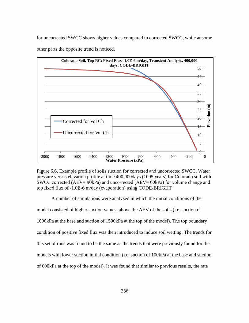
336
for uncorrected SWCC shows higher values compared to corrected SWCC, while at some
other parts the opposite trend is noticed.
Figure 6.6. Example profile of soils suction for corrected and uncorrected SWCC. Water
pressure versus elevation profile at time 400,000days (1095 years) for Colorado soil with
SWCC corrected (AEV= 90kPa) and uncorrected (AEV= 60kPa) for volume change and
top fixed flux of -1.0E-6 m/day (evaporation) using CODE-BRIGHT
A number of simulations were analyzed in which the initial conditions of the
model consisted of higher suction values, above the AEV of the soils (i.e. suction of
1000kPa at the base and suction of 1500kPa at the top of the model). The top boundary
condition of positive fixed flux was then introduced to induce soil wetting. The trends for
this set of runs was found to be the same as the trends that were previously found for the
models with lower suction initial condition (i.e. suction of 100kPa at the base and suction
of 600kPa at the top of the model). It was found that similar to previous results, the rate
0
5
10
15
20
25
30
35
40
45
50
-2000 -1800 -1600 -1400 -1200 -1000 -800 -600 -400 -200 0
Ele
va
tio
n (
m)
Water Pressure (kPa)
Colorado Soil, Top BC: Fixed Flux -1.0E-6 m/day, Transient Analysis, 400,000
days, CODE-BRIGHT
Corrected for Vol Ch
Uncorrected for Vol Ch
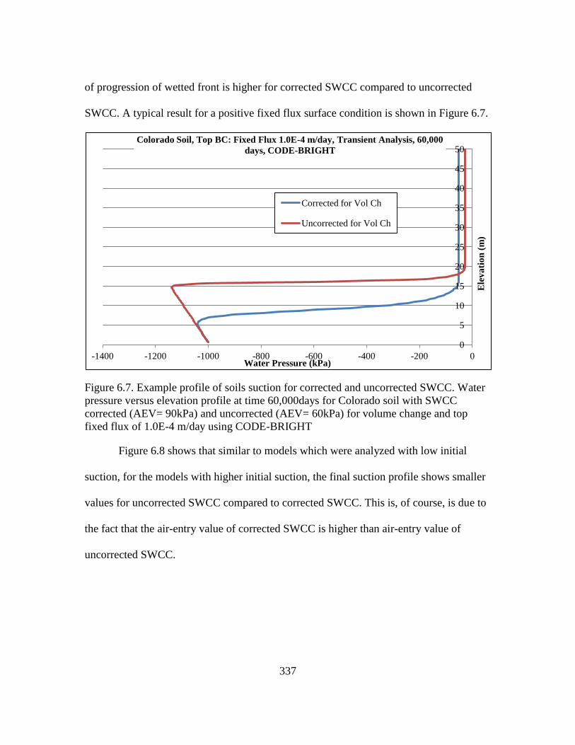
337
of progression of wetted front is higher for corrected SWCC compared to uncorrected
SWCC. A typical result for a positive fixed flux surface condition is shown in Figure 6.7.
Figure 6.7. Example profile of soils suction for corrected and uncorrected SWCC. Water
pressure versus elevation profile at time 60,000days for Colorado soil with SWCC
corrected (AEV= 90kPa) and uncorrected (AEV= 60kPa) for volume change and top
fixed flux of 1.0E-4 m/day using CODE-BRIGHT
Figure 6.8 shows that similar to models which were analyzed with low initial
suction, for the models with higher initial suction, the final suction profile shows smaller
values for uncorrected SWCC compared to corrected SWCC. This is, of course, is due to
the fact that the air-entry value of corrected SWCC is higher than air-entry value of
uncorrected SWCC.
0
5
10
15
20
25
30
35
40
45
50
-1400 -1200 -1000 -800 -600 -400 -200 0
Ele
va
tio
n (
m)
Water Pressure (kPa)
Colorado Soil, Top BC: Fixed Flux 1.0E-4 m/day, Transient Analysis, 60,000
days, CODE-BRIGHT
Corrected for Vol Ch
Uncorrected for Vol Ch
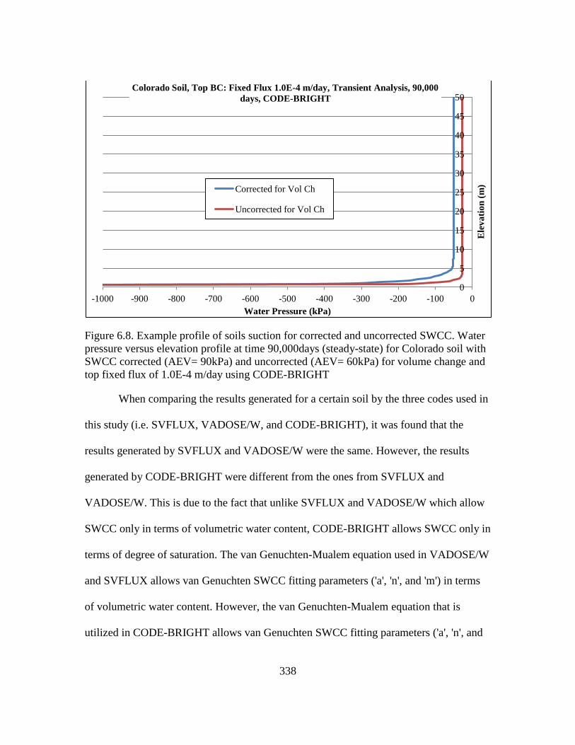
338
Figure 6.8. Example profile of soils suction for corrected and uncorrected SWCC. Water
pressure versus elevation profile at time 90,000days (steady-state) for Colorado soil with
SWCC corrected (AEV= 90kPa) and uncorrected (AEV= 60kPa) for volume change and
top fixed flux of 1.0E-4 m/day using CODE-BRIGHT
When comparing the results generated for a certain soil by the three codes used in
this study (i.e. SVFLUX, VADOSE/W, and CODE-BRIGHT), it was found that the
results generated by SVFLUX and VADOSE/W were the same. However, the results
generated by CODE-BRIGHT were different from the ones from SVFLUX and
VADOSE/W. This is due to the fact that unlike SVFLUX and VADOSE/W which allow
SWCC only in terms of volumetric water content, CODE-BRIGHT allows SWCC only in
terms of degree of saturation. The van Genuchten-Mualem equation used in VADOSE/W
and SVFLUX allows van Genuchten SWCC fitting parameters ('a', 'n', and 'm') in terms
of volumetric water content. However, the van Genuchten-Mualem equation that is
utilized in CODE-BRIGHT allows van Genuchten SWCC fitting parameters ('a', 'n', and
0
5
10
15
20
25
30
35
40
45
50
-1000 -900 -800 -700 -600 -500 -400 -300 -200 -100 0
Ele
va
tio
n (
m)
Water Pressure (kPa)
Colorado Soil, Top BC: Fixed Flux 1.0E-4 m/day, Transient Analysis, 90,000
days, CODE-BRIGHT
Corrected for Vol Ch
Uncorrected for Vol Ch
339
'm') in terms of degree of saturation only. It was established in Chapter 3, that for a given
expansive soil, the SWCC in terms of degree of saturation may have different fitting
parameters than the SWCC in terms of volumetric water content. The van Genuchten-
Mualem equation used in VADOSE/W and SVFLUX uses SWCC in terms of volumetric
water content and its saturated hydraulic conductivity and generates estimation for kunsat
function. In CODE-BRIGHT, however, the Van Genuchten-Mualem equation uses
SWCC in terms of degree of saturation (as opposed to volumetric water content in
VADOSE/W and SVFLUX). Therefore, the kunsat functions generated by VADOSE/W
and SVFLUX are the same but they are different from the kunsat functions generated by
CODE-BRIGHT. Figure 6.9 shows a comparison of results obtained from SVFLUX,
VADOSE/W, and CODE-BRIGHT for Colorado soil with top boundary condition of
5.0E-4 m/day. The figure shows reasonable agreement among the results obtained from
the three computer codes.
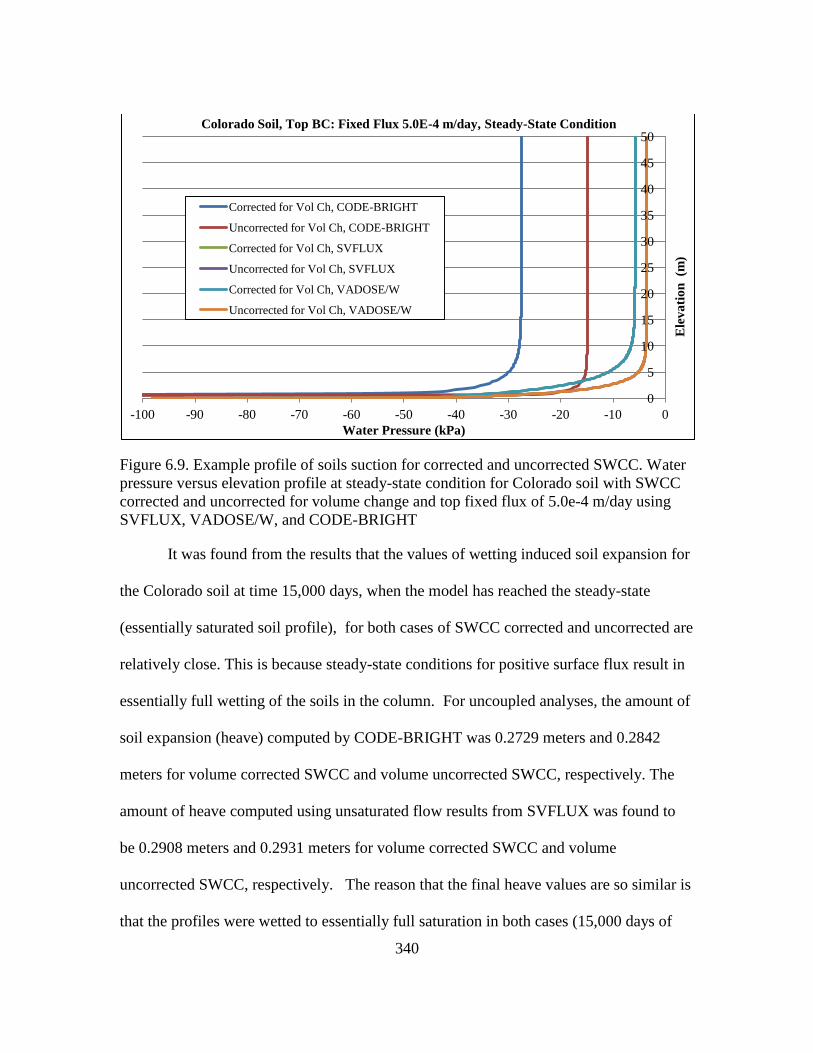
340
Figure 6.9. Example profile of soils suction for corrected and uncorrected SWCC. Water
pressure versus elevation profile at steady-state condition for Colorado soil with SWCC
corrected and uncorrected for volume change and top fixed flux of 5.0e-4 m/day using
SVFLUX, VADOSE/W, and CODE-BRIGHT
It was found from the results that the values of wetting induced soil expansion for
the Colorado soil at time 15,000 days, when the model has reached the steady-state
(essentially saturated soil profile), for both cases of SWCC corrected and uncorrected are
relatively close. This is because steady-state conditions for positive surface flux result in
essentially full wetting of the soils in the column. For uncoupled analyses, the amount of
soil expansion (heave) computed by CODE-BRIGHT was 0.2729 meters and 0.2842
meters for volume corrected SWCC and volume uncorrected SWCC, respectively. The
amount of heave computed using unsaturated flow results from SVFLUX was found to
be 0.2908 meters and 0.2931 meters for volume corrected SWCC and volume
uncorrected SWCC, respectively. The reason that the final heave values are so similar is
that the profiles were wetted to essentially full saturation in both cases (15,000 days of
0
5
10
15
20
25
30
35
40
45
50
-100 -90 -80 -70 -60 -50 -40 -30 -20 -10 0
Ele
va
tio
n (m
)
Water Pressure (kPa)
Colorado Soil, Top BC: Fixed Flux 5.0E-4 m/day, Steady-State Condition
Corrected for Vol Ch, CODE-BRIGHT
Uncorrected for Vol Ch, CODE-BRIGHT
Corrected for Vol Ch, SVFLUX
Uncorrected for Vol Ch, SVFLUX
Corrected for Vol Ch, VADOSE/W
Uncorrected for Vol Ch, VADOSE/W
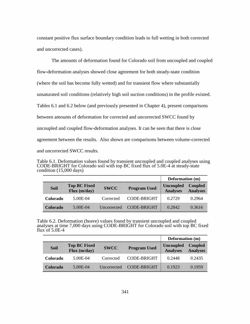
341
constant positive flux surface boundary condition leads to full wetting in both corrected
and uncorrected cases).
The amounts of deformation found for Colorado soil from uncoupled and coupled
flow-deformation analyses showed close agreement for both steady-state condition
(where the soil has become fully wetted) and for transient flow where substantially
unsaturated soil conditions (relatively high soil suction conditions) in the profile existed.
Tables 6.1 and 6.2 below (and previously presented in Chapter 4), present comparisons
between amounts of deformation for corrected and uncorrected SWCC found by
uncoupled and coupled flow-deformation analyses. It can be seen that there is close
agreement between the results. Also shown are comparisons between volume-corrected
and uncorrected SWCC results.
Table 6.1. Deformation values found by transient uncoupled and coupled analyses using CODE-BRIGHT for Colorado soil with top BC fixed flux of 5.0E-4 at steady-state condition (15,000 days)
Deformation (m)
Soil Top BC Fixed
Flux (m/day) SWCC Program Used
Uncoupled
Analyses
Coupled
Analyses
Colorado 5.00E-04 Corrected CODE-BRIGHT 0.2729 0.2964
Colorado 5.00E-04 Uncorrected CODE-BRIGHT 0.2842 0.3616
Table 6.2. Deformation (heave) values found by transient uncoupled and coupled analyses at time 7,000 days using CODE-BRIGHT for Colorado soil with top BC fixed flux of 5.0E-4
Deformation (m)
Soil Top BC Fixed
Flux (m/day) SWCC Program Used
Uncoupled
Analyses
Coupled
Analyses
Colorado 5.00E-04 Corrected CODE-BRIGHT 0.2448 0.2435
Colorado 5.00E-04 Uncorrected CODE-BRIGHT 0.1923 0.1959
342
It was found from the uncoupled and coupled flow-deformation analyses on
Colorado soil with top boundary condition of fixed flux of 5.0e-4 m/day that at time
7,000 days when the models has not reached the steady-state (not fully wetted), the
deformation (soil expansion) is significantly larger for corrected SWCC compared to
uncorrected SWCC (0.245m and 0.19m for corrected and uncorrected cases,
respectively). This is due to higher rate of progression of wetted front for the case of
corrected SWCC compared to uncorrected SWCC. The difference in deformation of
volume-corrected and volume-uncorrected cases were found to be insignificant at steady-
state condition where positive surface flux boundary conditions were applied, compared
to the earlier times in the process (i.e. when the soils have not become saturated), as
expected due to steady state conditions leading to essentially fully wetted conditions
(nearly zero suction). It was also found that for the conditions of fully wetted soils, the
deformation is slightly larger for volume-uncorrected SWCC (due to smaller suction
values within the profile) compared to volume-corrected SWCC resulting from difference
in the corrected and uncorrected curve AEV's. However, at times prior to steady-state
(when the soil is not saturated) the deformation was found to be larger for volume-
corrected SWCC because the water progresses more rapidly through the volume-
corrected soil profile case.
It should also be mentioned that for the expansive soils in this study, which do not
exhibit extreme volume change upon wetting and drying, the difference in the estimated
amounts of deformation for volume corrected and uncorrected SWCC's is not very large.
However, the difference observed here are expected to be substantially more pronounced
343
for more highly expansive soils (e.g. higher PI soils), for conditions resulting in larger
changes in soil suction, and also for any extremely high volume change soils, such as
slurry materials.
The effect of volume change on the shape of the SWCC, including AEV and
slope in the transition zone, is clearly demonstrated, and when volume change corrections
are not made, errors in the AEV and slope of the SWCC result. However, it is less clear
whether volume change corrections to the SWCC in estimating kunsat functions leads to
improved unsaturated flow results. The uncertainty results from the fact that the kunsat
function models have been developed using data that was not volume corrected. This may
lead to existence of compensating errors in the analyses. On the other hand, most of the
data used for developing and validating kunsat function models was not on clays, but rather
on silts, sands, and materials with no significant volume change. Therefore, correcting the
SWCC's for volume change may be a reasonable practice for soils with high volume
change potential (such as expansive soils and slurry specimens). More studies are needed
to evaluate the effect of volume change on SWCC key parameters, particularly AEV and
slope in transition zone, on the unsaturated flow properties (kunsat versus suction) of high
volume change soils. The study here on effects of volume change on SWCC's, kunsat
functions, and unsaturated flow/deformation analyses represents only a start on
understanding the complex issues at play for unsaturated flow/deformation modeling of
high volume change soils.
The SWCC's of oil sands tailings were previously established by Fredlund and
Houston (2013) and Fredlund et.al. (2011), by drying SWCC testing of the slurry
344
specimens. The initially saturated slurry specimens of oil sands tailings exhibit extreme
volume change upon increase in suction. Slurry specimens of oil sands tailings exhibit
shrinkage at suctions even smaller than air-entry value when the specimen is still
saturated. Volume changes at suction smaller than air-entry value affects the ksat value of
these specimens. The Kozeny-Carman is one method that can be used for correcting the
ksat at suctions smaller than air-entry value (Kozeny, 1927, and Carman, 1937, 1956).
However, none of the computer codes used in this study (i.e. VADOSE/W, SVFLUX,
and CODE-BRIGHT) has the capability to do corrections for ksat as the volume of the soil
changes at suctions smaller than the air-entry value. Therefore, as important as this
correction may be for slurry soils, it could not be accounted for in this study. The effect
of this ksat correction for compacted or native soil expansive clays is not expected to be
significant, whereas the effect of the ksat correction for suctions below the AEV would be
very substantial for slurry soils such as oil sands tailings. In addition to the points made
above, there are several reasons why the results on the oil sands tailings should not be
taken to be representative of any actual field condition. The most interesting field path for
oil sands tailings is drying from a slurry. In the field, the oil sands tailings start at
saturated conditions and then dry. For the simulations of this study, the oil sands tailings
were started at an initial condition of an unsaturated state and then either wetted or dried.
Further, the suction compression curve (void ratio versus suction) of oil sands tailings
obtained from previous research by Fredlund et al. (2011) was utilized, and in those
studies, a drying path was followed. For the cases in which a wetting path was simulated
in the numerical analyses for the oil sands tailings, no modification to the void ratio
345
versus suction relationship to account for difference in wetting and drying path were
made in this study.
Uncoupled (flow only) analyses on oil sands tailings were conducted for the
models based on properties of oil sands tailings in SVFLUX, VADOSE/W, and CODE-
BRIGHT in order to evaluate effect of volume-correcting SWCC on hydraulic properties
of soils and rate of changes in soil suction and the resulting suction-change induced
deformation. The rate of changes in soil suction was studied and amount of suction-
change induced deformation was determined based on the generated suction profile of the
soil column. The initial condition of the oil sand tailings was set to be unsaturated
(suction of 100kPa at the bottom and suction of 600kPa at the top of the model). For the
simulations in which the soil becomes wetted from the top by adding the positive fixed
flux, the suction of soil starts to decrease. It was previously established that the volume
corrected SWCC generally has larger AEV compared to the uncorrected SWCC. This
means that in the soil with volume corrected SWCC, desaturation starts at a larger suction
compared to the soil with uncorrected SWCC. That is to say, the soil with corrected
SWCC stays saturated at larger suction ranges compared to the soil with uncorrected
SWCC. Therefore, once the soil becomes wet and the suction decreases (i.e. wetting path
on the SWCC), for the soil with corrected SWCC, the soil becomes saturated (i.e. close to
AEV on SWCC) at a larger suction; whereas, the suction within the soil with uncorrected
SWCC should further decrease (compared to the soil with corrected SWCC) in order for
the suction to reach AEV (i.e. saturation or close-to-saturation state). This mechanism
illustrates the reason for the difference in final suction profile for the cases of volume
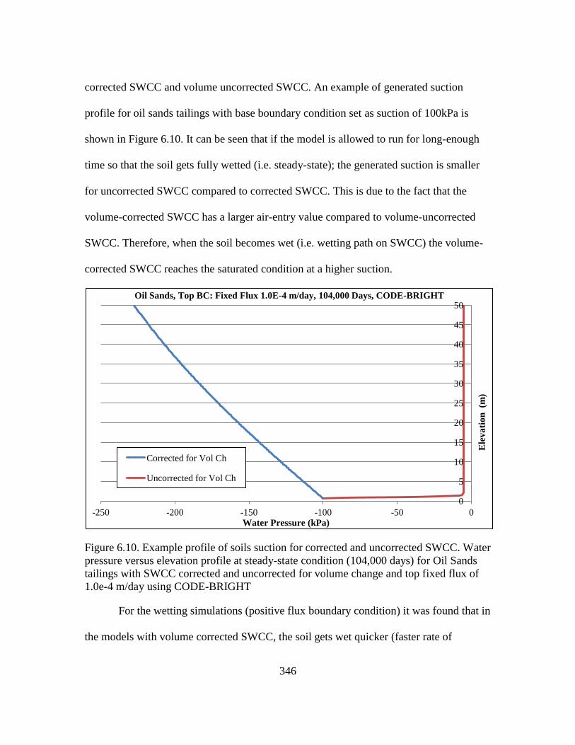
346
corrected SWCC and volume uncorrected SWCC. An example of generated suction
profile for oil sands tailings with base boundary condition set as suction of 100kPa is
shown in Figure 6.10. It can be seen that if the model is allowed to run for long-enough
time so that the soil gets fully wetted (i.e. steady-state); the generated suction is smaller
for uncorrected SWCC compared to corrected SWCC. This is due to the fact that the
volume-corrected SWCC has a larger air-entry value compared to volume-uncorrected
SWCC. Therefore, when the soil becomes wet (i.e. wetting path on SWCC) the volume-
corrected SWCC reaches the saturated condition at a higher suction.
Figure 6.10. Example profile of soils suction for corrected and uncorrected SWCC. Water
pressure versus elevation profile at steady-state condition (104,000 days) for Oil Sands
tailings with SWCC corrected and uncorrected for volume change and top fixed flux of
1.0e-4 m/day using CODE-BRIGHT
For the wetting simulations (positive flux boundary condition) it was found that in
the models with volume corrected SWCC, the soil gets wet quicker (faster rate of
0
5
10
15
20
25
30
35
40
45
50
-250 -200 -150 -100 -50 0
Ele
va
tio
n (m
)
Water Pressure (kPa)
Oil Sands, Top BC: Fixed Flux 1.0E-4 m/day, 104,000 Days, CODE-BRIGHT
Corrected for Vol Ch
Uncorrected for Vol Ch
347
progression of wetted front), as the unsaturated hydraulic conductivity of the soil with
corrected SWCC is higher than the unsaturated hydraulic conductivity of the same soil
with volume uncorrected SWCC. Larger values of kunsat results in water penetrating
through the soil faster.
For the times prior to the steady-state, in some portions of the soil profile, the
suction of uncorrected SWCC is higher than the suction of the corrected SWCC. This is
due to the fact that kunsat is generally higher for corrected SWCC and hence, at a given
time, the depth of wetting is generally larger for corrected SWCC compared to
uncorrected SWCC. Figure 6.11 shows an example which compares the depth of wetting
of volume-corrected and volume-uncorrected SWCC at the time 60,000 days for top
boundary condition of fixed flux of 1.0E-4 m/day for oil sands tailings. It can be seen that
the depth of wetting is larger for corrected SWCC (due to higher kunsat values). Figure
6.11 shows that at time 60,000 days the model with the volume-corrected SWCC has
reached the steady-state (fully wetted condition) while the model with the volume
corrected SWCC is only wetted half-way through the depth of column.
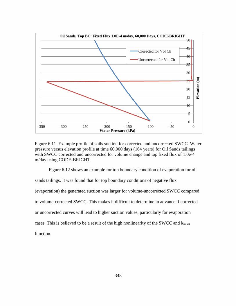
348
Figure 6.11. Example profile of soils suction for corrected and uncorrected SWCC. Water
pressure versus elevation profile at time 60,000 days (164 years) for Oil Sands tailings
with SWCC corrected and uncorrected for volume change and top fixed flux of 1.0e-4
m/day using CODE-BRIGHT
Figure 6.12 shows an example for top boundary condition of evaporation for oil
sands tailings. It was found that for top boundary conditions of negative flux
(evaporation) the generated suction was larger for volume-uncorrected SWCC compared
to volume-corrected SWCC. This makes it difficult to determine in advance if corrected
or uncorrected curves will lead to higher suction values, particularly for evaporation
cases. This is believed to be a result of the high nonlinearity of the SWCC and kunsat
function.
0
5
10
15
20
25
30
35
40
45
50
-350 -300 -250 -200 -150 -100 -50 0
Ele
va
tio
n (
m)
Water Pressure (kPa)
Oil Sands, Top BC: Fixed Flux 1.0E-4 m/day, 60,000 Days, CODE-BRIGHT
Corrected for Vol Ch
Uncorrected for Vol Ch
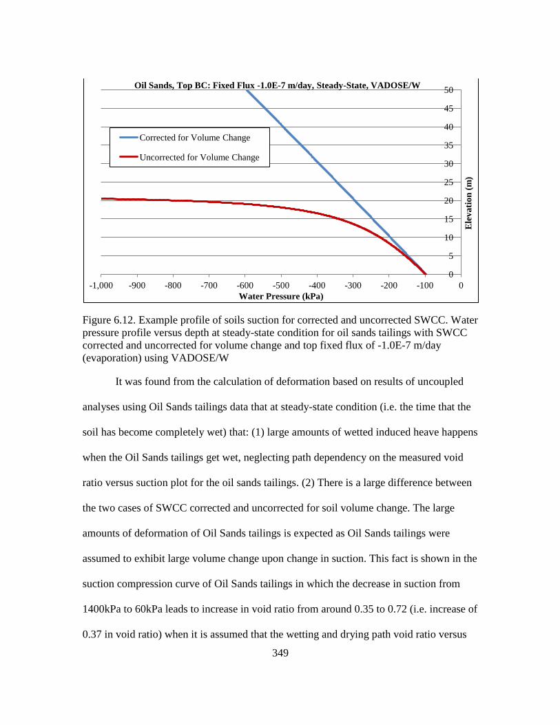
349
Figure 6.12. Example profile of soils suction for corrected and uncorrected SWCC. Water
pressure profile versus depth at steady-state condition for oil sands tailings with SWCC
corrected and uncorrected for volume change and top fixed flux of -1.0E-7 m/day
(evaporation) using VADOSE/W
It was found from the calculation of deformation based on results of uncoupled
analyses using Oil Sands tailings data that at steady-state condition (i.e. the time that the
soil has become completely wet) that: (1) large amounts of wetted induced heave happens
when the Oil Sands tailings get wet, neglecting path dependency on the measured void
ratio versus suction plot for the oil sands tailings. (2) There is a large difference between
the two cases of SWCC corrected and uncorrected for soil volume change. The large
amounts of deformation of Oil Sands tailings is expected as Oil Sands tailings were
assumed to exhibit large volume change upon change in suction. This fact is shown in the
suction compression curve of Oil Sands tailings in which the decrease in suction from
1400kPa to 60kPa leads to increase in void ratio from around 0.35 to 0.72 (i.e. increase of
0.37 in void ratio) when it is assumed that the wetting and drying path void ratio versus
0
5
10
15
20
25
30
35
40
45
50
-1,000 -900 -800 -700 -600 -500 -400 -300 -200 -100 0
Ele
va
tio
n (
m)
Water Pressure (kPa)
Oil Sands, Top BC: Fixed Flux -1.0E-7 m/day, Steady-State, VADOSE/W
Corrected for Volume Change
Uncorrected for Volume Change

350
suction curves are the same. This large amount of increase in void ratio leads to a large
amount of strain and thus heave. The final suction profile of the case in which SWCC is
uncorrected is much smaller than the suction within the Oil Sands tailings in the case of
the corrected SWCC. By using the same suction compression curve, much larger final
void ratio profile for the case with uncorrected SWCC is found compared to the case in
which SWCC is corrected. Larger final void ratio throughout the soil column leads to
more deformation at the column surface for the model with volume-uncorrected SWCC
(2.6m and 11.8m for corrected and uncorrected SWCC, respectively, were found by
uncoupled analyses using CODE-BRIGHT).
It was also found, as with the results on expansive soils, that depending upon the
time and amount of changes in soil suction (e.g. progression of wetted front) within the
profile, uncorrected SWCC may exhibit higher or lower suction compared to the
corrected SWCC. This makes it difficult to determine in advance if corrected or
uncorrected curves will lead to higher suction values, and further research is needed to
study this phenomenon from a fundamental unsaturated soil mechanics perspective.
6.3. Recommendations for Future Research
Based on the results of this study, the following recommendations for future
research are offered:
It is recommended that SWCC measurement devices which are capable of
accurate volume change measurement be developed. This type of device can
aid in more accurate measurement of dimensions of tested specimens which
leads to more accurate SWCC's. Existing oedometer-type pressure plate
351
devices as such a device, but present some challenges for drying path when
only light net normal stress is applied and for extremely high volume change
soils (e.g. slurry) when high suctions are applied.
It was found in this research, through literature review and laboratory testing,
that the SWCC in terms of degree of saturation best describes the unsaturated
properties of expansive soils. It is recommended that degree of saturation
representations for SWCC's be used for unsaturated flow analyses. It is
recommended that equations for predicting kunsat functions for clays
(particularly expansive clays) be developed which account for soil volume
change. Development of new formulations for kunsat functions for other high
volume change soils such as slurry soils and collapsible soils are also needed.
It was established that when volume change of slurry specimens may present
errors in predicting the ksat of this material, particularly for suctions smaller
than the air-entry value due to volume change that occurs under saturated
negative pore water pressure conditions. It is recommended that unsaturated
flow codes be enhanced to be able to do the necessary corrections to ksat when
simulating flows for slurry It is recommended to conduct numerical modeling
using a wider range of top boundary conditions fixed flux (both positive flux
and evaporation and more field-representative surface flux conditions), a
wider range of base boundary conditions head values, and a wider range of
material properties, including air-entry value and slope in transition zone.

352
Further research and studies on a wider range of high volume change soils is
needed. Flow and deformation analyses through uncoupled and coupled
flow/deformation numerical modeling for collapsible soils and other high
volume change soils should be done.
It is recommended that further study of the effect of net normal stress on
volume change of slurry specimens and other high volume change soil be
conducted with respect to SWCC be performed through laboratory testing.
353
REFERENCES
Abbaszadeh, M. (2011). The Effect of Cracks on Unsaturated Flow and Volume
Change Properties of Expansive Clays and Impacts on Foundation Performance.
Dissertation for Doctor of Philosophy. Arizona State University.
Abou-Bekr, N., Derdouf, F. M., and Bekkouche, A., (2005). “Behaviour Upon
Drying-wetting Paths of Maghnia Bentonite (West of Algeria). Proceedings of the
International Symposium Advanced Experimental Unsaturated Soil Mechanics, Experus
05, Tarantino et al., Eds., Balkema, pp. 145–169.
Aitchison, G.D., 1973. A quantitative description of the stress deformation
behavior of expansive soils, Proceedings, 3rd International Conference on Expansive
Soils, Haifa, vol. 2, pp. 79– 82.
Al-Mhaidib, A. I., 2008, Mathematical Model to Predict Swelling of Expansive
Soil, the 12th International Conference of International Association for Computer
Methods and Advances in Geomechanics (IACMAG)
Al-Shamrani, M. A. and Dhowian A. W., 2003, Experimental study of lateral
restraint effects on the potential heave of expansive soils, Engineering Geology 69, pp
63–81
Al-Zoubi, M. Sh., 2008, Swell Characteristics of Natural and Treated Compacted
Clays, EJGE
American Society for Testing and Materials (ASTM) (2007) “Standard Test
Method for Particle-Size Analysis of Soils", ASTM D422 - 63(2007)
American Society for Testing and Materials (ASTM) (2010) “Standard Test
Methods for Specific Gravity of Soil Solids by Water Pycnometer", ASTM D854 - 10
American Society for Testing and Materials (ASTM) (2010) “Standard Test
Methods for Liquid Limit, Plastic Limit, and Plasticity Index of Soils", ASTM D4318 -
10
American Society for Testing and Materials (ASTM) (2010) "Standard Test
Method for Measurement of Soil Potential (Suction) Using Filter Paper" ASTM D5298 -
10
American Society for Testing and Materials (ASTM) (2012) “Standard Test
Methods for Laboratory Compaction Characteristics of Soil Using Standard Effort",
ASTM D698 - 12
Barbour S. L. (1998). The soil-water characteristic curve: a historical perspective.
Canadian Geotechnical Journal 35, 873-894.
354
Baumgartl, T., Rostek, J., Horn, R., (2000). Internal and external stresses
affecting the water retention curve. Advances in GeoEcology 32: 13-21
Biarez, J., Fleureau, J. M., Zerhouni, M. I., and Soepandji, B. S. (1987).
“Variations de volumes des sols argileux lors de cycles de drainage humidification.” Rev.
Fr. Géotech., 41: 63–71.
Bilsel, h., (2004), Hydraulic properties of soils derived from marine sediments of
Cyprus, Journal of Arid Environments 56 (2004) 27–41
Brooks, R. H., and Corey, A. T. (1964). “Hydraulic properties of porous media.”
Hydrology Paper No. 3, Colorado State Univ., Fort Collins, Colo.
Brutsaert, W. (1967). “Some methods of calculating unsaturated permeability.”
Trans. ASAE, 10, 400–404.
Buckingham, E. (1907). “Studies of the Movement of Soil Moisture.” U.S.D.A.
Bur. Of Soils, Bulletin No. 38.
Bulut, R. and Wray, W. K. (2005). “Free Energy of Water-Suction-in Filter
Papers.” Geotechnical Testing Journal, 28(4), 1 – 10.
Bulut, R., Lytton, R. L., and Wray, W. K. (2001). “Soil Suction Measurements by
Filter Paper.” Proceedings of Geo-Institutes Shallow Foundation and Soil Properties
Committee Sessions at the ASCE 2001 Civil Engineering Conference, Houston, Texas.
October 10-31, 243 – 261.
Burdine, N. (1953). Relative permeability calculations from pore-size distribution
data, Pet. Trans. Am. Inst. of Mining and Met. Eng. 198, 71-77
Cabral, A.R., Planchet, L., Marinho, F.A., and Lefebvre, G. 2004. Determination
of the soil water characteristic curve of highly compressible materials: Case study of pulp
and paper by-product. Geotechnical Testing Journal, 27: 154–162.
Campbell, G. S. (1974). “A simple method for determining unsaturated
conductivity from moisture retention data.” Soil Sci., 117(6), 311–314.
Campbell, J.D. (1973). Pore pressures and volume changes in unsaturated soils.
Ph.D. thesis, University of Illinois at Urbana- Champaign, Urbana-Champaign, Ill.
Celia, M.A., and Bouloutas, E.T., (1990) A general mass-conservative numerical
solution for the unsaturated flow equation. Water Resources Research, Vol. 26, No 7, pp.
1483-1496, July.
Chandler R.J. and Gutierrez C.I. (1986). The filter paper method of suction
measurement. Geotechnique, 36, pp- 265 -268.
355
Chao, K. C. (1995). “Hydraulic Properties and Heave Prediction for Expansive
Soil.” Maters Thesis, Colorado State University, Fort Collins, Colorado.
Chao, K. C. (2007), Design Principles For Foundations On Expansive Soils, PhD
Dissertation, Colorado State University, Fort Collins, Colorado
Chao, K. C., Durkee, D. B., Miller, D. J., and Nelson, J. D. (1998). “Soil Water
Characteristic Curve for Expansive Soil.” Thirteenth Southeast Asian Geotechnical
Conference, Taipei, Taiwan.
Chao, K.C., Nelson, J.D., Overton, D.D., and Cumbers, J.M. (2008), Soil water
retention curves for remolded expansive soils, Unsaturated Soils: Advances in Geo-
Engineering- Toll et al. (eds): 243-248
Chertkov, V.Y. (2004). A physically based model for the water retention curve of
clay pastes. Journal of Hydrology, 286: 203– 226. doi:10.1016/j.jhydrol.2003.09.019.
Childs, E., and Collis-George. N. (1950). The permeability of porous materials.
Proc. Roy. Soc. London. A: 201, 392-405.
Ching, R. K. H. and Fredlund, D. G. (1984). “A Small Saskatchewan Town Copes
with Swelling Clay Problems.” Proc. 5th Int. Conf. Expansive Soils, 306 – 310.
Chiu, C. F., Ng, C. W. W., (2012), Coupled water retention and shrinkage
properties of a compacted silt under isotropic and deviatoric stress paths, Can. Geotech. J.
49: 928–938, doi:10.1139/T2012-055
Code_Bright Pre-Process, Problem Data (2012). CODE-BRIGHT Manual
Cokca, E,. 2000, Comparison of suction and oedometer methods for the
measurement of swell pressure, Quarterly Journal of Engineering Geology and
Hydrology, 33, pp 141-147
Çokca, E. 2002, Relationship between methylene blue value, initial soil suction,
and swell percent of expansive soil. Turkish J. Eng. Env. Sci. 26 , 521–529.
Croney D. 1952. The movement and distribution of water in soil. Géotechnique. 3
(1), 1-16.
Croney, D., and Coleman, J.D., (1961). Pore pressure and suction in soils.
Proceedings, Conference on Pore Pressures and Suction in Soils. Butterworths, London.
Pp. 31-37
Cui, Y., Mantho, A., Cui, K., Audiguier, M., (2006), Water retention properties
and volume change behavior of natural Romainville clay. Unsaturated Soils, pp: 873- 882
356
Darcy, H. (1856). “Les fontaines publiques de la ville de Dijon.” V. Dalmont,
Paris, 647
Delage, P., Suraj De Silva G.P.R., De Laure, E., (1987). Un nouvel appareil
triaxial pour les sols non satures. Comptes-rendus de la lome Conf. europeene de
Mecanique des Sols et des Travaux de Fooundation, Dublin, vol. 1: 26-28
Dye, H. B., (2008). Moisture movement through expansive soil and impact on
performance of residential structures, PhD Dissertation, Arizona State University
Ebrahimi-B, N., Gitirana, G. F. N., Jr., Fredlund, D. G., Fredlund, M. D., and
Samarasekera, L. (2004). “A lower limit for the water permeability coefficient.” Proc.,
57th Canadian Geotechnical Conf., Vol. 1, Quebec City, Que., Canada, 12–19.
Eching, S. and Hopmans, J. (1993). Optimization of hydraulic functions from
transient outflow and soil water pressure data. SSSAJ. 57, 1167-1175.
Edgar, T. V., Nelson, J. D., and McWhorter, D. B. (1989).“Nonisothermal
Consolidation in Unsaturated Soil.” The Journal of Geotechnical Engineering, 115(10),
1351 – 1372.
Elrick, E. C., and Bowman, D. H., (1964). Note on an improved apparatus for soil
flow moisture measurements. Soil Sci. Soc. Amer. Proc. 28: 450-453
Erzin Y., and Erol O., 2007, Swell pressure prediction by suction methods,
Engineering Geology 92, pp133–145
Farrel, D. A., and Larson, W. E. (1972). “Modeling the pore structure of porous
media.” Water Resour. Res., 8(3), 699–706.
Feng, M., and Fredlund, D. G. (1999). “Hysteretic influence associated with
thermal conductivity sensor measurements.” Proc., 52nd Canadian Geotechnical Conf.,
Regina, Sask., Canada, 651–657.
Fernandez-Galvez, J., Barahona, E. (2006). Changes in water retention due to soil
kneading. Journal of Agricultural water management, Elsevier B. V. No. 76. P. 53-61.
Fleureau, J. M., Kheirbek-Saoud, S., Soemitro, R., and Taibi, S. (1993).
“Behavior of clayey soils on drying-wetting paths.” Can. Geotech. J., 30: 287–296.
Fleureau, J. M., Verbrugge, J. C., Huergo, P. J., Correia, A. G., and Kheirbek-
Saoud, S. (2002). “Aspects of the behaviour of compacted clayey soils on drying and
wetting paths.” Can. Geotech. J., 39: 1341–1356.
Fleureau, J.M., Hadiwarrdoyo, S., and Kheirbek-Saoud, S. (2004). Simplified
approach to the behavior of compacted soils on drying and wetting paths. In Proceedings
357
of the Third International Conference on Unsaturated Soils, Recife, Brazil, 10–13 March
2002. Edited by J.F.T. Juca, T.M.P. de Campos, and F.A.M. Marinho. A.A. Balkema,
Lisse, the Netherlands.
Fleureau, J.M., Kheirbek-Saoud, S., and Taibi, S. (1995). Experimental aspects
and modeling of the behaviour of soils with a negative pressure. In Proceedings of the 1st
International Conference on Unsaturated Soils, Paris, France, 6–8 September 1995,
Edited by X. Alonso and X. Delage. A.A. Balkema, Rotterdam, the Netherlands. Vol. 1.
pp. 57–62.
Fredlund, D. G. (2000). “The 1999 R.M. Hardy Lecture: The Implementation of
Unsaturated Soil Mechanics into Geotechnical Engineering.” Canadian Geotechnical
Journal, 37, 963 – 986.
Fredlund, D. G. (2002). “Use of Soil-Water Characteristic Curves in the
Implementation of Unsaturated Soil Mechanics.” Third International Conference on
Unsaturated Soils. Recife, Brazil.
Fredlund, D. G. and Rahardjo, H. (1993). Soil mechanics for unsaturated soils.
New York: Wiley.
Fredlund, D. G., and Morgenstern, N. R. (1977). “Stress state variables for
unsaturated soils.” J. Geotech. Eng. Div., Am. Soc. Civ. Eng., 103(5), 447–466.
Fredlund, D. G., and Rahardjo, H. (1993). “The role of unsaturated soil behavior
in geotechnical practice.” Proc., 11th Southeast Asian Geotechnical Conference, Invited
Keynote Address, Singapore, 37–49.
Fredlund, D. G., and Xing, A. (1994). “Equations for the soil-water characteristic
curve.” Can. Geotech. J., 31(4), 521–532.
Fredlund, D. G., Houston, S. L. (2009). Protocol for the assessment of unsaturated
soil properties in geotechnical engineering practice, Can. Geotech. J. 46: 694–707.
doi:10.1139/T09-010
Fredlund, D. G., Houston, S. L., (2013). Interpretation of Soil-Water
Characteristic Curves when Volume Change Occurs as Soil Suction is Changed, Pan-
American Conference on Unsaturated Soils, Cartagena de Indias, Colombia
Fredlund, D. G., Sheng, D., Zhao, J. (2011). Estimation of soil suction from the
soil-water characteristic curve. Can. Geotech. J. 48: 186–198. doi:10.1139/T10-060
Fredlund, D. G., Shuai, F., and Feng, M. (2000). “Increased accuracy in suction
measurement using an improved thermal conductivity sensor.” Proc., 7th Int. Conf. on
Tailings and Mine Waste, Fort Collins, Colo., 443–450.
358
Fredlund, D. G., Xing, A., and Huang, S. (1994). Predicting the permeability
function for unsaturated soils using the soil-water characteristic curve. Canadian
Geotechnical Journal, 31(4), pp 533–546
Fredlund, D.G. (1964). Comparison of soil suction and one-dimensional
consolidation characteristics of highly plastic clay. M.Sc. thesis, University of Alberta,
Edmonton, Alta.
Fredlund, D.G., Stone, J., Stianson, J., (2011), Determination of Water Storage
and Permeability Functions for Oil Sands Tailings, Proceedings Tailings and Mine Waste
2011, Vancouver, BC, November 6 to 9, 2011
Fredlund. D.G. (2006). Unsaturated Soil Mechanics in Engineering Practice,
Journal of Geotechnical and Geoenvironmental Engineering, Vol. 132, No. 3, 286- 321
Fredlund, M. D., Fredlund, D. G., Houston, S. L., Houston, W. (2003).
Assessment of unsaturated soil properties for seepage modeling through tailings and mine
wastes. Tailings and Mine Waste '03, Swets and Zeitlinger, Lisses
Frost, J. D. and Park, J. Y. (2003). “A Critical Assessment of the Moist Tamping
Technique.” ASTM Geotechnical Testing Journal, 26(1), 57 – 70.
Gallipoli, D., Gens, A., Sharma, R., and Vaunat, J. (2003). “An elastoplastic
model for unsaturated soil incorporating the effects of suction and degree of saturation on
mechanical behaviour.” Geotechnique, 53(1), 123–135.
Gallipoli, D., Gens, A., Vaunat, J., and Romero, E. (2002). Role of degree of
saturation on the normally consolidated behavior of unsaturated soils. Experimental
evidence and theoretical approaches in unsaturated soils, A. Tarantino and C. Mancuso,
eds, Balkema, Rotterdam, The Netherlands: 115–120.
Gallipoli, D., Wheeler, S. J., and Karstunen, M. (2003). Modeling the variation of
degree of saturation in a deformable unsaturated soil. Geotechnique, 53(1): 105–112.
Gardner W. (1958). Some steady-state solutions of the unsaturated moisture flow
equation with applications to evaporation from a water table. Soil Sci. 85, 228-232.
Gardner, W. (1958). “Mathematics of isothermal water conduction in unsaturated
soils.” Highway Research Board Special Rep. No. 40, Int. Symp. on Physico-Chemical
Phenomenon in Soils, Washington, D.C. pp. 78–87.
Gardner, W. R. (1956). “Calculation of capillary conductivity from pressure plate
outflow data.” Soil Sci. Soc. Am. Proc., 20: 317–320.
GEO-SLOPE International Ltd. (2012). Vadose Zone Modeling with
VADOSE/W, an Engineering Methodology
359
Geotechnical Consulting and Testing Systems, Inc. (GCTS). (2004). “Fredlund
SWCC Device Operating Instructions.” Tempe, Arizona.
Gillham, R. W., Klute, A., and Heerman, D. F., (1976) Hydraulic properties of a
porous medium: measurement and empirical representation. Soil Sci. Soc. Am. J. 40, No.
2, 203-207
Green , R. E., Hanks, R. J., Larson, W. E. (1964). Estimates of field infiltration by
numerical solution of the moisture flow equation, Soil. Sci. Soc. Amer. Proc. 28: 15-19
Green, R.E. and Corey, J.C., (1971) Calculation of Hydraulic Conductivity: A
Further Evaluation of Some Predictive Methods. Soil Science Society of America
Proceedings, Vol. 35, pp. 3-8.
Head, K.H. (1980). Manual of soil laboratory testing: soil classification and
compaction tests. Pentech Press, London.
Hilf, J. W. (1956). “An investigation of pore-water pressure in compacted
cohesive soils.” Technical Memorandum No. 654,PhD thesis, Design and Construction
Division, Bureau of Reclamation, United States Department of the Interior, Denver.
Hillel, D., 1980. Fundamentals of Soil Physics, Academic, San Diego, Calif.
Holtz, R. D., Kovacs, W. D., Sheahan, T. C. (2010). An Introduction to
Geotechnical Engineering (2nd Edition). Prentice Hall;
Houston, S. L., Houston, W. R., and Wagner, A. M. (1994). “Laboratory Filter
Paper Measurements.” Geotechnical Testing Journal, 17(2), 185 – 194.
Huang, S.Y., Barbour, S.L., and Fredlund, D.G. 1998. Development and
verification of a coefficient of permeability function for a deformable unsaturated soil.
Canadian Geotechnical Journal, 35: 411–425. doi:10.1139/cgj-35-3-411.
Ito, M., Azam, S., (2010), Determination of Swelling and Shrinkage Properties of
Undisturbed Expansive Soils, Geotech Geol Eng (2010) 28:413–422
Jacquemin, S., 2011. Laboratory determination of hydraulic conductivity
functions for unsaturated cracked fine grained soil. Thesis for Master of Science. Arizona
State University.
James M., Tinjum, Craig, H., Benson, Lisa, R., and Blotz (1997) “Soil-water
characteristic curves for compacted clays.” Journal of Geotechnical and Geo-
environmental engineering
Jian Z., Jian-lin Y. (2005). Influences affecting the soil-water characteristic curve.
Journal of Zhejan Iniversity Science. 6A(8): 797-804.
360
Johnson, L.D., Snethen, D.R., 1978. Prediction of potential heave of swelling
soils, Geotechnical Testing Journal, ASTM 1 (3), 117– 124
Jury, W. A., Gardner, W. R., and Gardner, W. H. (1991). “Soil Physics, Fifth
Edition.” John Wiley & Sons, Inc., New York, NY.
Kassiff, G., and Benshalom, A. (1971), Experimental relationship between swell
pressure and suction. Geotechnique 21: 245-255
Komornik, A. and David, D. (1969) Prediction of swelling pressure of clays: J.
ASCE, Soil Mechanics and Foundation Division, SM No. 1, pp. 209-225.
Kunze, R.J., Vehara, G., and Graham, K., (1968). Factors Important in the
Calculation of Hydraulic Conductivity. Soil Science of America Proceedings, Soil
Physics, Vol. 32
Ladd, R. S. (1978). “Preparing Test Specimens Using Undercompaction.” ASTM
Geotechnical Testing Journal, 1(1), 16 – 23.
Laliberte, G. E. (1969). “A mathematical function for describing capillary
pressure-desaturation data.” Bull. Int. Assoc. Sci. Hydrol., 14(2), 131–149.
Leong E., C., and Rahardjo, H. Permeability Functions for Unsaturated Soils.
1997 Journal of Geotechnical and Geoenvironmental Engineering, 123, (12): 1118-1126.
Leong, E. C. and Rahardjo, H. (1997). “Review of Soil-Water Characteristic
Curve Equations.” Journal of Geotechnical and Geoenvironmental Engineering, 123(12),
1106 – 1117.
Leong, E. C., He, L., and Rahardjo, H. (2002). “Factors Affecting the Filter Paper
Method for Total and Matric Suction Measurements.” Geotechnical Testing Journal,
25(3), 322 – 333.
Li, J., Sun, D.A., Sheng, D.C., Sloan, S. and Fredlund, D. (2007) Preliminary
Study on Soil-Water Characteristics of Maryland Clay, Proc. 3rd Asian Conf. on
Unsaturated Soils, Nanjing, China (ed. Z.Z. Yin, J.P. Yuan & A.C.F. Chiu), Beijing:
Science Press, pp. 569-574.
Li, J.Y., Yang, Q., Li, P. Y., Yang, Q. L., (2009), Experimental Research on Soil-
Water Characteristic Curve of Remolded Residual Soils, EJGE, Vol. 14 [2009], Bund. L
Lins, Y., and Schanz, T. (2004). “Determination of hydro-mechanical properties
of sand.” Int. Conf. on Experimental Evidence towards Numerical Modeling of
Unsaturated Soils, T. Schanz, ed., Lecture Notes in Applied Mechanics, Springer, New
York, 11–29.
361
Liu, Q., Yasufuku, N., Omine, K., Hazarike, H., (2012), Automatic soil water
retention test system with volume change measurement for sandy and silty soils, Soils
and Foundations 52 (2): 368-380
Liu, Q., Yasufuku, N., Omine, K., Kobayashi, T., (2011), Automatic soil water
retention testing system with volume change measurement, Deformation Characteristics
of Geomaterials
Lytton, R.L., (1977). The characterization of expansive soils in engineering,
Presentation at the Symposium on Water Movement and Equilibrium in Swelling Soils,
American Geophysical Union, San Francisco, CA
Lytton, R.L., 1994. Prediction of movement in expansive clays, In Proceedings of
Vertical and Horizontal Deformations of Foundations and Embankments, Geotechnical
Special Publication No. 40, ASCE, New York, pp. 1827–1845
Marshall, T.J. (1958). A relation between permeability and size distribution of
pores. Journal of Soil Science, 9: 1 8.
Mbonimpa, M., Aubertin, M., Maqsoud, A., Bussière, B., (2006), Predictive
Model for the Water Retention Curve of Deformable Clayey Soils, Journal of
Geotechnical and Geoenvironmental Engineering, Vol. 132, No. 9: 1121- 1132
McCartney, J.S., Villar, L. F. S., Zornberg, J.G. (2007). Estimation of the
Hydraulic Conductivity Function of Unsaturated Clays Using Infiltration Column Tests.
NSAT- Volume 1- Parte 2.
McKee, C., and Bumb, A. (1987). “Flow-testing coalbed methane production
wells in the presence of water and gas.” Proc., 1985 SPE Formation Evaluation Paper
SPE 14447, Society of Petroleum Engineers, Richardson, Tex., 599–608.
McKee, C.R., and Bumb, A.C. 1984. The importance of unsaturated flow
parameters in designing a monitoring system for hazardous wastes and environmental
emergencies. In Proceedings of the Hazardous Materials Control Research Institute
National Conference, Houston, Tex., March 1984. pp. 50–58.
McKeen, R. G. (2001) “Investigating Field Behavior of Expansive Clay Soils”,
Expansive Clay Soils and Vegetative Influence on Shallow Foundations, Proceedings of
Geo-Institute Shallow Foundation and Soil Properties Committee Sessions at the ASCE
2001 Civil Engineering Conference, Houston, Texas, Geotechnical Special Publication
No. 115, 82-94.
McQueen, I. S. and Miller, R. F. (1968). “Calibration and Evaluation of Wide
Range Gravimetric Method for Measuring Soil Moisture Stress.” Soil Science, 10, 521 –
527.
362
Millington, R. J., and Quirk, J. P. (1959). Transport in porous media. Int. Cong.
Soil Sci., Trans. 7th
(Madison, Wis.) 1.3: 97-106
Millington, R.J., and Quirk, J.P., (1961). Permeability of Porous Solids.
Transaction of the Faraday Society, Vol. 57, pp. 1200-1207
Moore, R.E. (1939). Water conduction from shallow water tables. Hilgardia, 12:
383-426.
Mualem, Y. (1976) .A new model for predicting the hydraulic conductivity of
unsaturated porous media, WRR 12,513-522
Mualem, Y. (1976). Hysteretical models for prediction of the hydraulic
conductivity of unsaturated porous media. Water Resources Research, 12: 1248-1 254.
Muir Wood, D. (1991). Soil Behaviour and Critical State Soil Mechanics,
Cambridge [England] ; New York : Cambridge University Press
Mulilis, J. P., Chan, C. K., and Seed, H. B. (1975). “The Effects of Method of
Sample Preparation on the Cyclic Stress Strain Behavior of Sands.” EERC Report, 75 –
78.
Nagaraj, T. S. and Murthy, B. R. (1985) “Prediction of the Pre-consolidation
Pressure and Recompression Index of Soils”, Geotechnical Testing Journal, ASTM, 8(4),
pp. 199–202.
Nayak, N.V., and Christensen, R.W. 1971, Swell characteristics of compacted
expansive soils, Clays and clay minerals 19, 251-261
Nelson, J. D. (1985). “Constitutive Relationships and Testing of Unsaturated
Soils.” Proceedings of the Eleventh International Conference on Soil Mechanics and
Foundation Engineering, San Francisco.
Nelson, J. D. and Miller, D. J. (1992). “Expansive Soils: Problems and Practice in
Foundation and Pavement Engineering.” John Wiley & Sons, Inc., New York, NY.
Nelson, J. D., Overton, D. D., and Durkee, D. B. (2001). “Depth of Wetting and
the Active Zone.” Expansive Clay Soils and Vegetative Influence on Shallow
Foundations, ASCE, Houston, Texas. 95 – 109.
Ng, C.W.W., and Pang, Y.W. (2000). Influence of stress state on soil-water
characteristics and slope stability. Journal of Geotechnical and Geoenvironmental
Engineering, 126(2): 157–166. doi:10. 1061/(ASCE)1090-0241(2000)126:2(157)
363
Ng, C.W.W., Lai, C.H., and Chiu, C.F. (2012). A modified triaxial apparatus for
measuring the stress path-dependent water retention curve. Geotechnical Testing Journal,
35(3): 490–495. doi:10.1520/ GTJ104203.
Nielsen D. R., Davidson, J. M., Biggar, J. W., and Miller R.J., (1964). Water
movement through Panoche clay loam soil. Hilgardia 35: 491-506
Noorany, I. (1992). Discussion of “Stress Ratio on Collapse of Compacted Clayey
Sand.” by Lawton, E. C., Fragaszy, R. J., and Hardcastle, J. H., 1991, Journal of
Geotechnical Engineering, 117(5), 714 – 730.
Noorany, I. (2005). E-Mail Letter to Kuo-Chieh Chao Regarding “Moist Tamping
Equipment.” January 10th.
Nuth, M., Laloui, L. (2008). Advances in modelling hysteretic water retention
curve in deformable soils. Computers and Geotechnics 35 (2008) 835–844.
doi:10.1016/j.compgeo.2008.08.001
Nuth, M., Laloui, L., (2011), A model for the water retention behavior of
deformable soils including capillary hysteresis, Geo-Frontiers, ASCE, pp 3896-3905
Oliveira, O. M. and Fernando, F. A. M. (2006). “Evaluation of Filter Paper
Calibration.” Proceedings of the Fourth International Conference on Unsaturated Soils.
Carefree, Arizona. 1845 – 1851.
Olivella, S., A. Gens, J. Carrera, E. E. Alonso, (1996), Numerical Formulation for
a Simulator (CODE_BRIGHT) for the Coupled Analysis of Saline Media, Engineering
Computations, Vol. 13, No 7, , pp: 87-112.
Olivella, S., J. Carrera, A. Gens, E. E. Alonso, (1994). Non-isothermal Multiphase
Flow of Brine and Gas through Saline media. Transport in Porous Media, 15, 271:293
Olivella, S., J. Carrera, A. Gens, E. E. Alonso. (1996) Porosity Variations in
Saline Media Caused by Temperature Gradients Coupled to Multiphase Flow and
Dissolution/Precipitation. Transport in Porous Media, 25:1-25.
Olson, R. and Daniel, D. (1981). Measurement of the Hydraulic Conductivity of
Fine Grained Soils, ASTM STP 746, 18-64.
O'Neil, M.W., and Gazzaly, O.I. 1977, Swell potential related to building
performance, Journal of the Geotechnical Engineering Division, ASCE 103 (12), 1363 –
1379
Pachepsky, Y., Timlin, D., Rawls, W. (2003). Generalized Richards’ equation to
simulate water transport in unsaturated soils, Journal of Hydrology 272, pp. 3–13
364
Parent, S. E., Cabral, A., Zornberg, J. G., (2007). Water retention curve and
hydraulic conductivity function of highly compressible materials. Canadian Geotech.
Journal 44: 1200–1214, doi:10.1139/T07-091
Parker, J., Kool, J., and van Genuchten, M. (1985). Determining soil hydraulic
properties from one- step outflow experiments by parameter estimation: II
Experimental studies. SSSAJ. 49,1354-1359.
Pe´ron, H., Hueckel, T., and Laloui, L. (2007). An improved volume
measurement for determining soil water retention curves. Geotechnical Testing Journal,
Vol. 30, No. 1: 1–8.
Pereira, J.H.F., and Fredlund, D.G. 2000. Volume change behaviour of a residual
soil of gneiss compacted at metastable structured conditions. Journal of Geotechnical and
Geoenvironmental Engineering, 126(10): 907–916. doi:10.1061/(ASCE) 1090-
0241(2000)126:10(907).
Perera, Y. Y., Padilla, J. M., and Fredlund, D. G. (2004). “Determination of Soil-
water Characteristic Curves Using the Fredlund SWCC Device.” Tailings and Mine
Waste Management Short Course, Vail, Colorado. October.
Perez-Garcia, N., Houston, S. L., Houston, W. N., and Padilla, J. M. (2008). An
Oedometer-Type Pressure Plate SWCC Apparatus, Geotechnical Testing Journal (GTJ) /
Citation Page, Volume 31, Issue 2 (March 2008),ISSN: pp 1945-7545
Perko, H. A., Thompson, R. W., Nelson, J. D., (2000). Suction Compression
Index Based on CLOD Test Results. GeoDenver 2000 Advances in Unsaturated
Geotechnics, 10.1061/40510(287)27
Pham, H. Q., Fredlund, D. G. (2008). Equations for the entire soil-water
characteristic curve of a volume change soil. Can. Geotech. J. 45: 443–453.
doi:10.1139/T07-117
Pham, H. Q., Fredlund, D. G., Barbour, A. L. (2003). Estimation of the hysteretic
soil-water characteristic curves from the boundary drying curve. 56TH Canadian
Geotechnical Conference, 4TH Joint Iah-Cnc/Cgs Conference
Pham, H. Q., Fredlund, D. G., Barbour, S. L. (2003). A practical hysteresis model
for the soil-water characteristic curve for soils with negligible volume change.
Geotechnique 53, No. 2, 293-298
Pham, H.Q. (2001). An engineering model of hysteresis for soil water
characteristic curves. M.Sc. thesis, University of Saskatchewan, Saskatoon, Sask.
Pham, Q.H. 2005. A volume-mass constitutive model for unsaturated soils. Ph.D.
dissertation, University of Saskatchewan, Saskatoon, Sask.
365
Powers, K. C., Vanapalli, S. K. and Garga, V. K. (2007). New and improved null
pressure plate apparatus for the measurement of matric suction of unsaturated soils.
Canadian Geotechnical Conference, Ottawa, Ontario, Canada.
Price, J.S., and Schlotzhauer, S.M. 1999. Importance of shrinkage and
compression in determining water storage changes in peat: the case of a mined peat land.
Hydrological Processes, 13: 2591– 2601. doi:10.1002/(SICI)1099
Qi, G., Michel J. C., (2011) A laboratory device for continual measurement of
water retention and shrink/swell properties during drying/wetting cycles. HortScience 46
(9): 1298-1302
Rahardjo, H. and Leong, E.C., 2006. Suction Measurements, In Proceedings of
Fourth International Conference of Unsaturated Soils, Carefree, Arizona, pp. 81-104.
Ranganatham, B. V. and Satyanarayan, B. (1965), A rational method of predicting
swelling potential for compacted expansive clays: Proc. 6th Inter. Conf. Soil Mechanics
Foundation Engng. Vol. 1, pp. 92-96
Rao A.S., Phanikumar B.R. and Sharma R.S., 2004, Prediction of swelling
characteristics of remoulded and compacted expansive soils using free swell index,
Quarterly Journal of Engineering Geology and Hydrogeology, 37, 217–226
Reginato, R. J., and van Bavel, C. H. M. (1962). “Pressure cell for soil cores.”
Soil Sci. Soc. Am. Proc., 26, 1–3.
Richard, R. M., and B. J. Abbott 1975, Versatile elastic-plastic stress-strain
formula, Journal of Engineering Mechanics, ASCE, 10(4,) 511-515
Richards, B.G. (1965). Measurement of the free energy of soil moisture by the
psychrometric technique using thermistors. In Moisture equilibria and moisture changes
in soils beneath covered areas. Edited by G.D. Aitchison. Butterworths, Australia. pp. 39-
46.
Richards, L.A., 1931. Capillary conduction of liquids in porous mediums, Physics
1, 318–333
Rogowski, A. S. (1971). Watershed physics: Model of the soil moisture
characteristic. Water Resources Research 7(6): 1575-1582.
Romero, E., Gens, A., Lloret, A. (1999). Water permeability, water retention and
microstructure of unsaturated compacted Boom clay. Engineering Geology 54 (1999)
117–127
Saaltink, M. W., Ayora, C., Olivella S., (2005). User's guide for
RetrasoCodeBright (RCB)
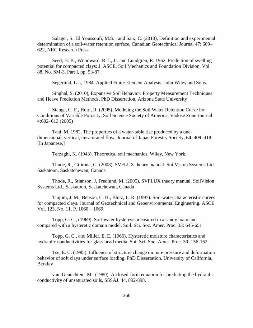
366
Salager, S., El Youssoufi, M.S. , and Saix, C. (2010), Definition and experimental
determination of a soil-water retention surface, Canadian Geotechnical Journal 47: 609–
622, NRC Research Press
Seed, H. B., Woodward, R. J., Jr. and Lundgren, R. 1962, Prediction of swelling
potential for compacted clays: J. ASCE, Soil Mechanics and Foundation Division, Vol.
88, No. SM-3, Part I, pp. 53-87.
Segerlind, L.J., 1984. Applied Finite Element Analysis. John Wiley and Sons.
Singhal, S. (2010), Expansive Soil Behavior: Property Measurement Techniques
and Heave Prediction Methods, PhD Dissertation, Arizona State University
Stange, C. F., Horn, R. (2005), Modeling the Soil Water Retention Curve for
Conditions of Variable Porosity, Soil Science Society of America, Vadose Zone Journal
4:602–613 (2005)
Tani, M. 1982. The properties of a water-table rise produced by a one-
dimensional, vertical, unsaturated flow. Journal of Japan Forestry Society, 64: 409–418.
[In Japanese.]
Terzaghi, K. (1943). Theoretical soil mechanics, Wiley, New York.
Thode, R., Gitirana, G. (2008). SVFLUX theory manual. SoilVision Systems Ltd.
Saskatoon, Saskatchewan, Canada
Thode, R., Stianson, J, Fredlund, M. (2005). SVFLUX theory manual, SoilVision
Systems Ltd., Saskatoon, Saskatchewan, Canada
Tinjum, J. M., Benson, C. H., Blotz, L. R. (1997). Soil-water characteristic curves
for compacted clays. Journal of Geotechnical and Geoenvironmental Engineering. ASCE.
Vol. 123, No. 11. P. 1060 – 1069.
Topp, G. C., (1969). Soil-water hysteresis measured in a sandy loam and
compared with a hysteretic domain model. Soil. Sci. Soc. Amer. Proc. 33: 645-651
Topp, G. C., and Miller, E. E. (1966). Hysteretic moisture characteristics and
hydraulic conductivities for glass bead media. Soil Sci. Soc. Amer. Proc. 30: 156-162.
Tse, E. C. (1985). Influence of structure change on pore pressure and deformation
behavior of soft clays under surface loading. PhD Dissertation. University of California,
Berkley
van Genuchten, M. (1980). A closed-form equation for predicting the hydraulic
conductivity of unsaturated soils, SSSAJ. 44, 892-898.
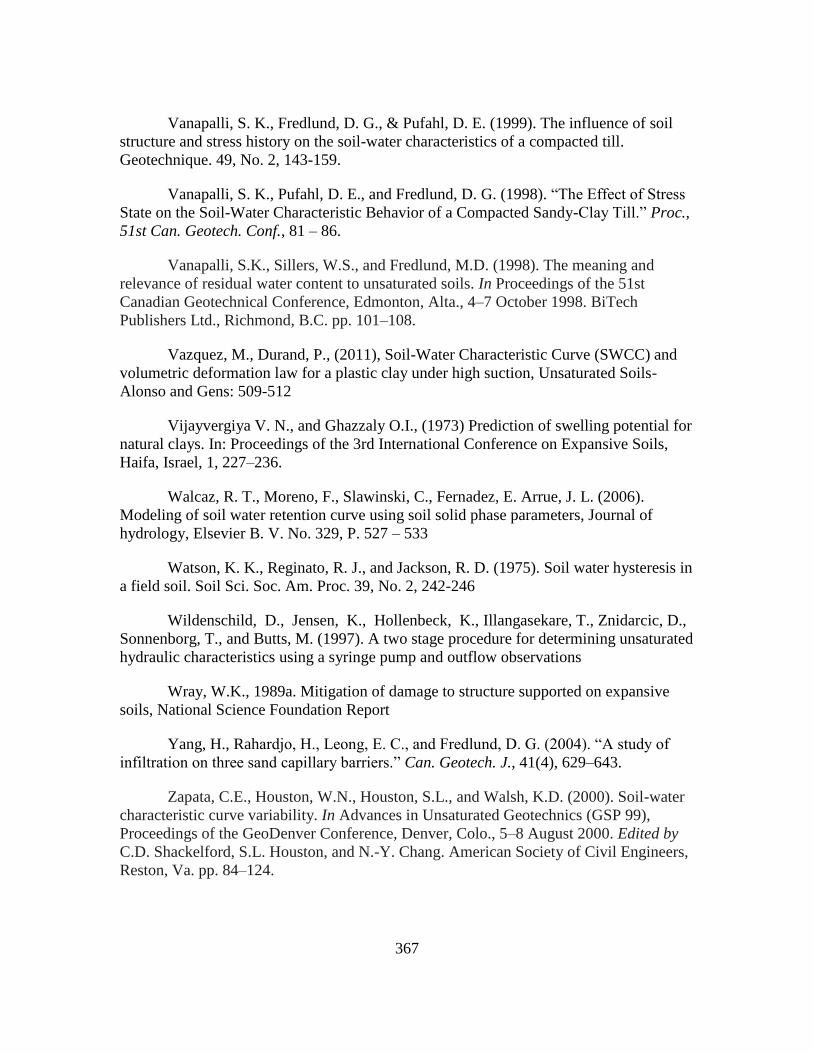
367
Vanapalli, S. K., Fredlund, D. G., & Pufahl, D. E. (1999). The influence of soil
structure and stress history on the soil-water characteristics of a compacted till.
Geotechnique. 49, No. 2, 143-159.
Vanapalli, S. K., Pufahl, D. E., and Fredlund, D. G. (1998). “The Effect of Stress
State on the Soil-Water Characteristic Behavior of a Compacted Sandy-Clay Till.” Proc.,
51st Can. Geotech. Conf., 81 – 86.
Vanapalli, S.K., Sillers, W.S., and Fredlund, M.D. (1998). The meaning and
relevance of residual water content to unsaturated soils. In Proceedings of the 51st
Canadian Geotechnical Conference, Edmonton, Alta., 4–7 October 1998. BiTech
Publishers Ltd., Richmond, B.C. pp. 101–108.
Vazquez, M., Durand, P., (2011), Soil-Water Characteristic Curve (SWCC) and
volumetric deformation law for a plastic clay under high suction, Unsaturated Soils-
Alonso and Gens: 509-512
Vijayvergiya V. N., and Ghazzaly O.I., (1973) Prediction of swelling potential for
natural clays. In: Proceedings of the 3rd International Conference on Expansive Soils,
Haifa, Israel, 1, 227–236.
Walcaz, R. T., Moreno, F., Slawinski, C., Fernadez, E. Arrue, J. L. (2006).
Modeling of soil water retention curve using soil solid phase parameters, Journal of
hydrology, Elsevier B. V. No. 329, P. 527 – 533
Watson, K. K., Reginato, R. J., and Jackson, R. D. (1975). Soil water hysteresis in
a field soil. Soil Sci. Soc. Am. Proc. 39, No. 2, 242-246
Wildenschild, D., Jensen, K., Hollenbeck, K., Illangasekare, T., Znidarcic, D.,
Sonnenborg, T., and Butts, M. (1997). A two stage procedure for determining unsaturated
hydraulic characteristics using a syringe pump and outflow observations
Wray, W.K., 1989a. Mitigation of damage to structure supported on expansive
soils, National Science Foundation Report
Yang, H., Rahardjo, H., Leong, E. C., and Fredlund, D. G. (2004). “A study of
infiltration on three sand capillary barriers.” Can. Geotech. J., 41(4), 629–643.
Zapata, C.E., Houston, W.N., Houston, S.L., and Walsh, K.D. (2000). Soil-water
characteristic curve variability. In Advances in Unsaturated Geotechnics (GSP 99),
Proceedings of the GeoDenver Conference, Denver, Colo., 5–8 August 2000. Edited by
C.D. Shackelford, S.L. Houston, and N.-Y. Chang. American Society of Civil Engineers,
Reston, Va. pp. 84–124.

368
Zerhouni, M. I., (1991). Rôle de la pression interstitielle négative dans le
comportement des sols Application au calcul des routes, Ph.D. Thesis, Ecole Nationale
des Ponts et Chaussées, Paris.
Zhou, J. & Yu, J. (2005). Influences affecting the soil-water characteristic curve",
Journal of Zhejiang University SCIENCE, 6A(8): 797-804.

369
APPENDIX A
IMAGES OF SOIL SPECIMENS TESTED BY SWC-150 DEVICE
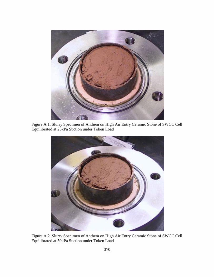
370
Figure A.1. Slurry Specimen of Anthem on High Air Entry Ceramic Stone of SWCC Cell
Equilibrated at 25kPa Suction under Token Load
Figure A.2. Slurry Specimen of Anthem on High Air Entry Ceramic Stone of SWCC Cell
Equilibrated at 50kPa Suction under Token Load
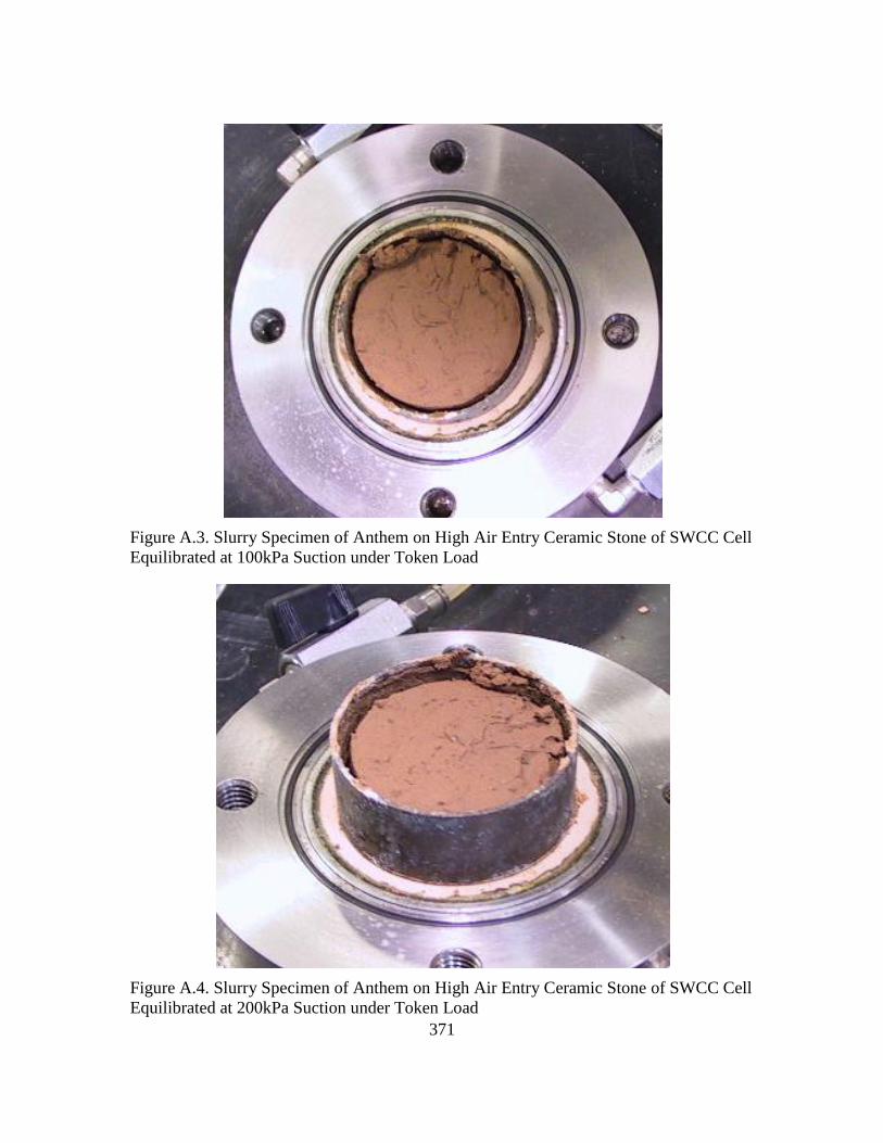
371
Figure A.3. Slurry Specimen of Anthem on High Air Entry Ceramic Stone of SWCC Cell
Equilibrated at 100kPa Suction under Token Load
Figure A.4. Slurry Specimen of Anthem on High Air Entry Ceramic Stone of SWCC Cell
Equilibrated at 200kPa Suction under Token Load
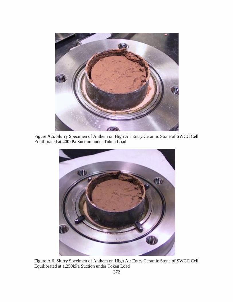
372
Figure A.5. Slurry Specimen of Anthem on High Air Entry Ceramic Stone of SWCC Cell
Equilibrated at 400kPa Suction under Token Load
Figure A.6. Slurry Specimen of Anthem on High Air Entry Ceramic Stone of SWCC Cell
Equilibrated at 1,250kPa Suction under Token Load
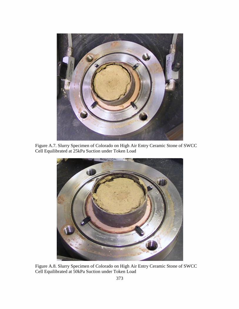
373
Figure A.7. Slurry Specimen of Colorado on High Air Entry Ceramic Stone of SWCC
Cell Equilibrated at 25kPa Suction under Token Load
Figure A.8. Slurry Specimen of Colorado on High Air Entry Ceramic Stone of SWCC
Cell Equilibrated at 50kPa Suction under Token Load
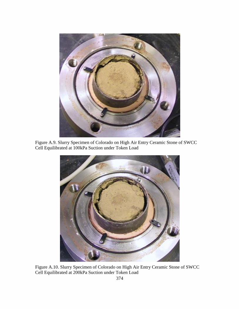
374
Figure A.9. Slurry Specimen of Colorado on High Air Entry Ceramic Stone of SWCC
Cell Equilibrated at 100kPa Suction under Token Load
Figure A.10. Slurry Specimen of Colorado on High Air Entry Ceramic Stone of SWCC
Cell Equilibrated at 200kPa Suction under Token Load
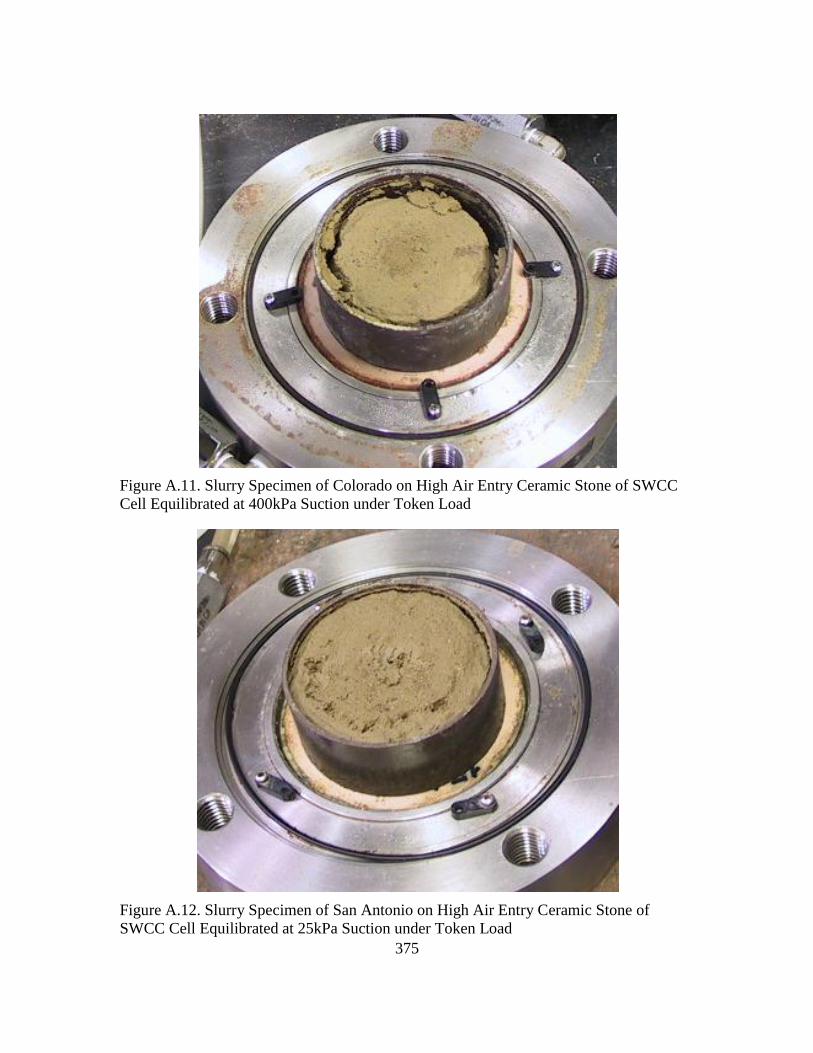
375
Figure A.11. Slurry Specimen of Colorado on High Air Entry Ceramic Stone of SWCC
Cell Equilibrated at 400kPa Suction under Token Load
Figure A.12. Slurry Specimen of San Antonio on High Air Entry Ceramic Stone of
SWCC Cell Equilibrated at 25kPa Suction under Token Load
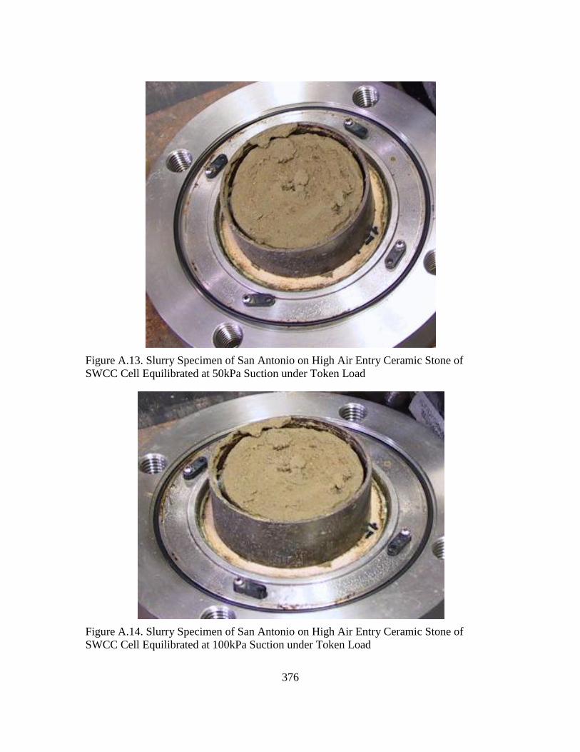
376
Figure A.13. Slurry Specimen of San Antonio on High Air Entry Ceramic Stone of
SWCC Cell Equilibrated at 50kPa Suction under Token Load
Figure A.14. Slurry Specimen of San Antonio on High Air Entry Ceramic Stone of
SWCC Cell Equilibrated at 100kPa Suction under Token Load
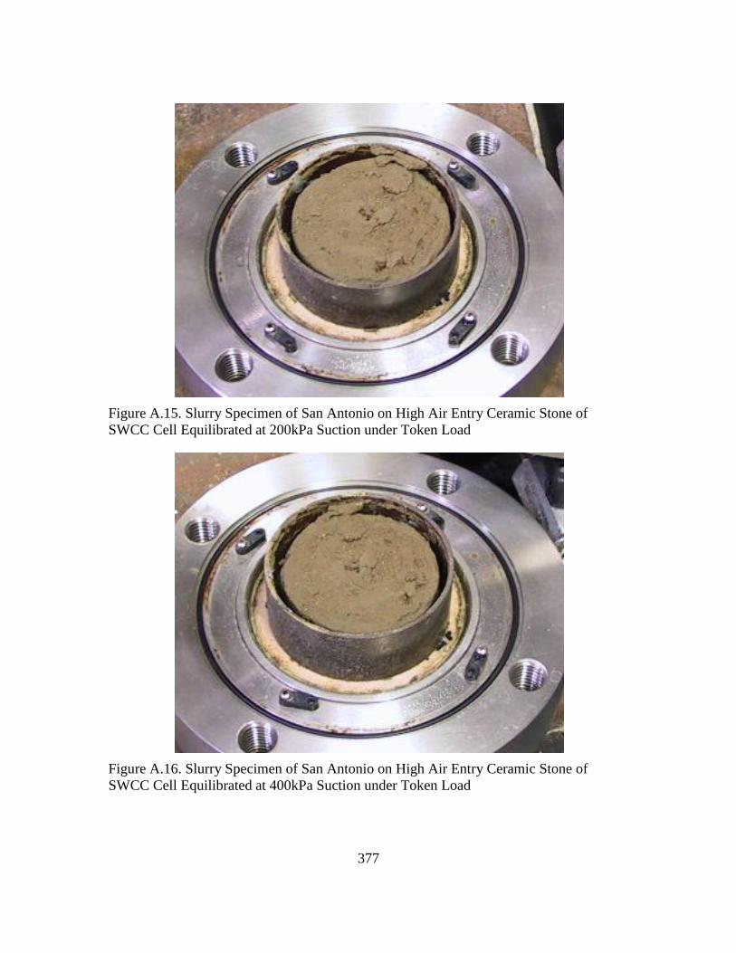
377
Figure A.15. Slurry Specimen of San Antonio on High Air Entry Ceramic Stone of
SWCC Cell Equilibrated at 200kPa Suction under Token Load
Figure A.16. Slurry Specimen of San Antonio on High Air Entry Ceramic Stone of
SWCC Cell Equilibrated at 400kPa Suction under Token Load
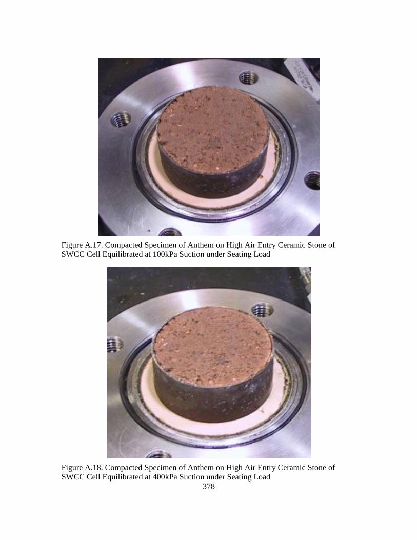
378
Figure A.17. Compacted Specimen of Anthem on High Air Entry Ceramic Stone of
SWCC Cell Equilibrated at 100kPa Suction under Seating Load
Figure A.18. Compacted Specimen of Anthem on High Air Entry Ceramic Stone of
SWCC Cell Equilibrated at 400kPa Suction under Seating Load
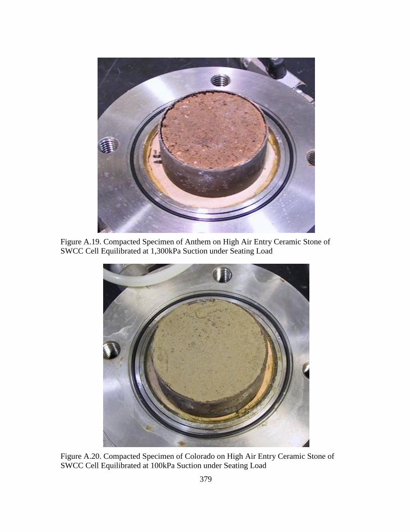
379
Figure A.19. Compacted Specimen of Anthem on High Air Entry Ceramic Stone of
SWCC Cell Equilibrated at 1,300kPa Suction under Seating Load
Figure A.20. Compacted Specimen of Colorado on High Air Entry Ceramic Stone of
SWCC Cell Equilibrated at 100kPa Suction under Seating Load
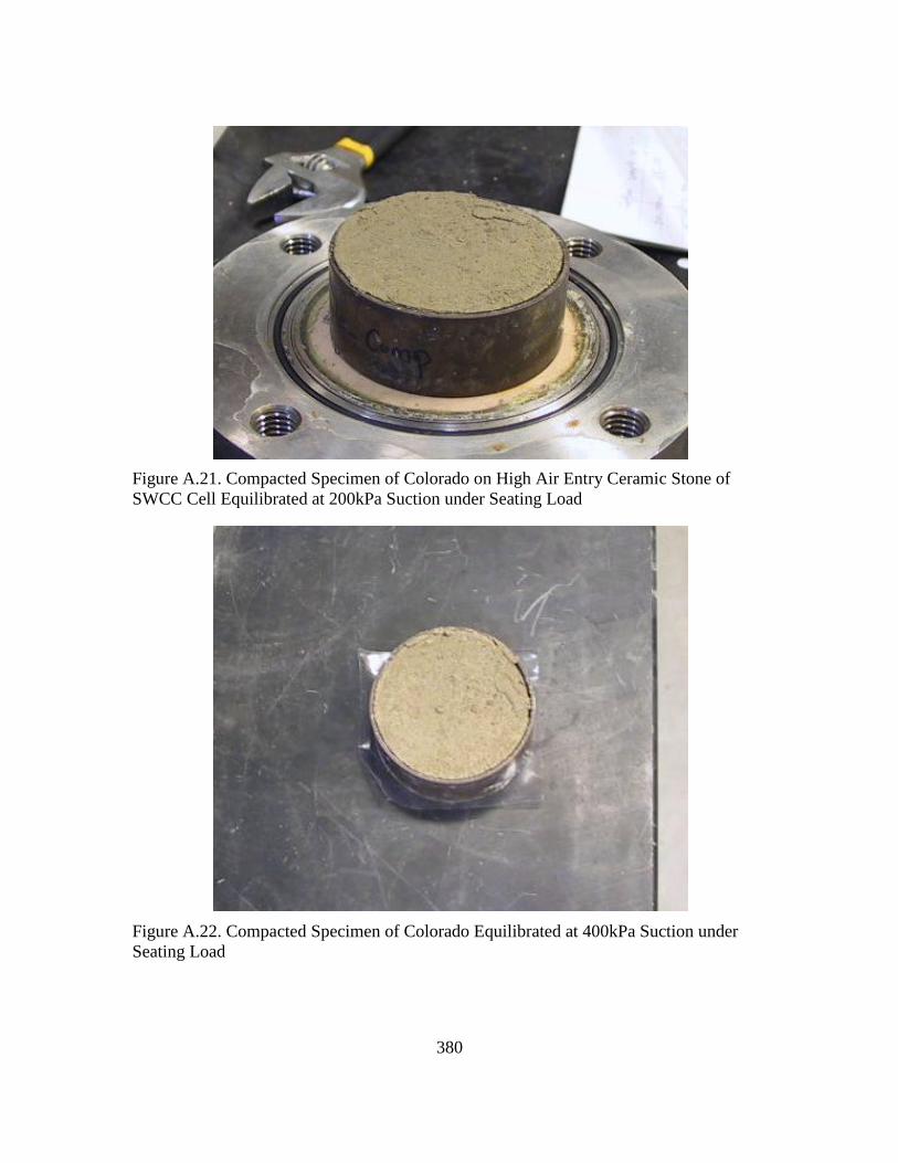
380
Figure A.21. Compacted Specimen of Colorado on High Air Entry Ceramic Stone of
SWCC Cell Equilibrated at 200kPa Suction under Seating Load
Figure A.22. Compacted Specimen of Colorado Equilibrated at 400kPa Suction under
Seating Load
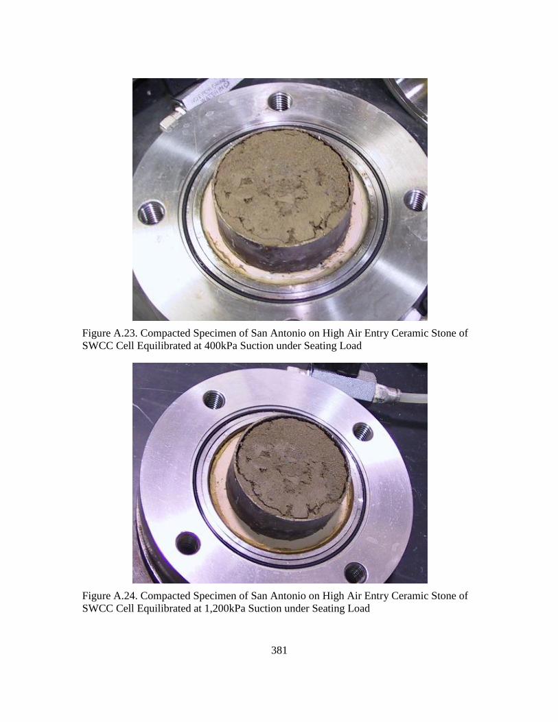
381
Figure A.23. Compacted Specimen of San Antonio on High Air Entry Ceramic Stone of
SWCC Cell Equilibrated at 400kPa Suction under Seating Load
Figure A.24. Compacted Specimen of San Antonio on High Air Entry Ceramic Stone of
SWCC Cell Equilibrated at 1,200kPa Suction under Seating Load
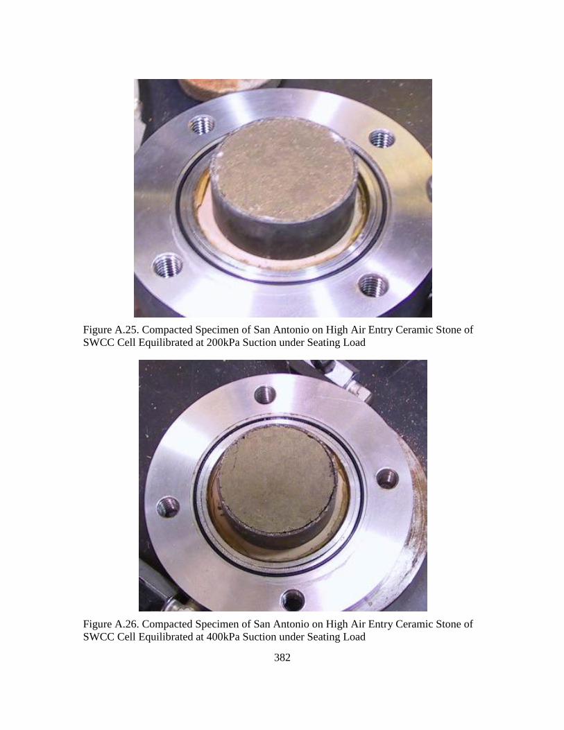
382
Figure A.25. Compacted Specimen of San Antonio on High Air Entry Ceramic Stone of
SWCC Cell Equilibrated at 200kPa Suction under Seating Load
Figure A.26. Compacted Specimen of San Antonio on High Air Entry Ceramic Stone of
SWCC Cell Equilibrated at 400kPa Suction under Seating Load
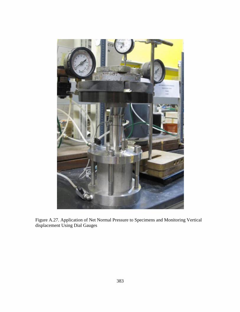
383
Figure A.27. Application of Net Normal Pressure to Specimens and Monitoring Vertical
displacement Using Dial Gauges
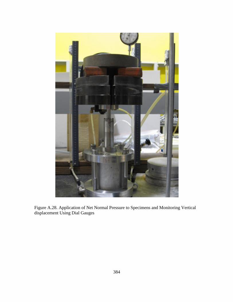
384
Figure A.28. Application of Net Normal Pressure to Specimens and Monitoring Vertical
displacement Using Dial Gauges

385
APPENDIX B
RESULTS OF NUMERICAL MODELING: PROFILES OF SOILS SUCTION FOR
CORRECTED AND UNCORRECTED SWCC'S
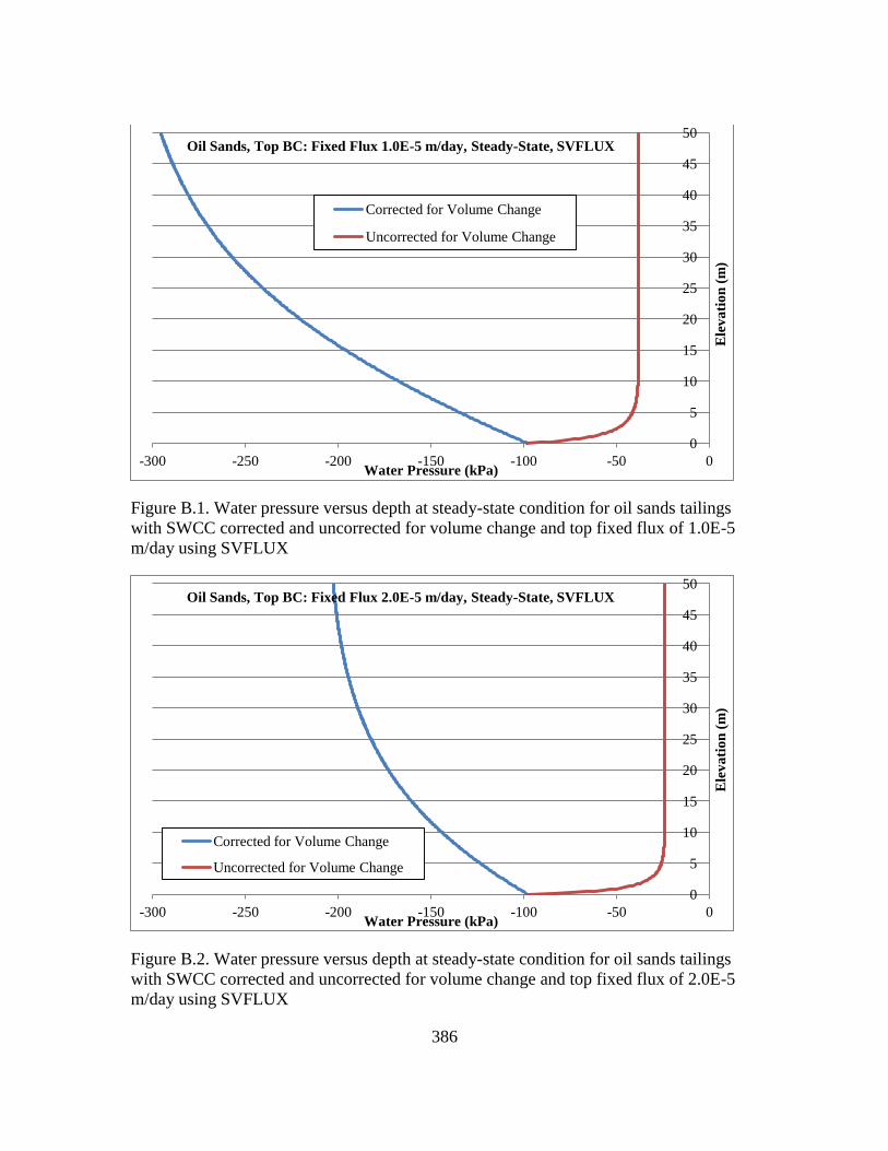
386
Figure B.1. Water pressure versus depth at steady-state condition for oil sands tailings
with SWCC corrected and uncorrected for volume change and top fixed flux of 1.0E-5
m/day using SVFLUX
Figure B.2. Water pressure versus depth at steady-state condition for oil sands tailings
with SWCC corrected and uncorrected for volume change and top fixed flux of 2.0E-5
m/day using SVFLUX
0
5
10
15
20
25
30
35
40
45
50
-300 -250 -200 -150 -100 -50 0
Ele
va
tio
n (
m)
Water Pressure (kPa)
Oil Sands, Top BC: Fixed Flux 1.0E-5 m/day, Steady-State, SVFLUX
Corrected for Volume Change
Uncorrected for Volume Change
0
5
10
15
20
25
30
35
40
45
50
-300 -250 -200 -150 -100 -50 0
Ele
va
tio
n (
m)
Water Pressure (kPa)
Oil Sands, Top BC: Fixed Flux 2.0E-5 m/day, Steady-State, SVFLUX
Corrected for Volume Change
Uncorrected for Volume Change
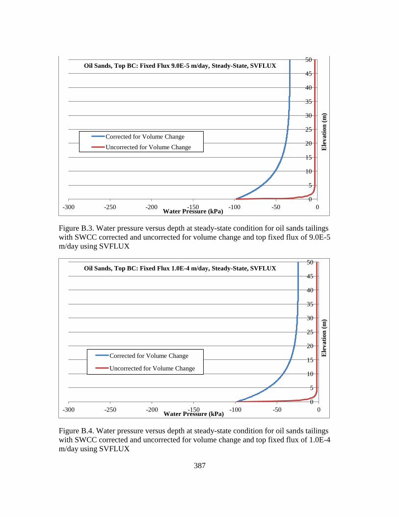
387
Figure B.3. Water pressure versus depth at steady-state condition for oil sands tailings
with SWCC corrected and uncorrected for volume change and top fixed flux of 9.0E-5
m/day using SVFLUX
Figure B.4. Water pressure versus depth at steady-state condition for oil sands tailings
with SWCC corrected and uncorrected for volume change and top fixed flux of 1.0E-4
m/day using SVFLUX
0
5
10
15
20
25
30
35
40
45
50
-300 -250 -200 -150 -100 -50 0
Ele
va
tio
n (
m)
Water Pressure (kPa)
Oil Sands, Top BC: Fixed Flux 9.0E-5 m/day, Steady-State, SVFLUX
Corrected for Volume Change
Uncorrected for Volume Change
0
5
10
15
20
25
30
35
40
45
50
-300 -250 -200 -150 -100 -50 0
Ele
va
tio
n (
m)
Water Pressure (kPa)
Oil Sands, Top BC: Fixed Flux 1.0E-4 m/day, Steady-State, SVFLUX
Corrected for Volume Change
Uncorrected for Volume Change
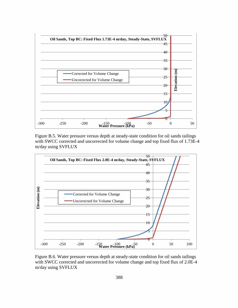
388
Figure B.5. Water pressure versus depth at steady-state condition for oil sands tailings
with SWCC corrected and uncorrected for volume change and top fixed flux of 1.73E-4
m/day using SVFLUX
Figure B.6. Water pressure versus depth at steady-state condition for oil sands tailings
with SWCC corrected and uncorrected for volume change and top fixed flux of 2.0E-4
m/day using SVFLUX
0
5
10
15
20
25
30
35
40
45
50
-300 -250 -200 -150 -100 -50 0 50
Ele
va
tio
n (
m)
Water Pressure (kPa)
Oil Sands, Top BC: Fixed Flux 1.73E-4 m/day, Steady-State, SVFLUX
Corrected for Volume Change
Uncorrected for Volume Change
0
5
10
15
20
25
30
35
40
45
50
-300 -250 -200 -150 -100 -50 0 50 100
Ele
va
tio
n (
m)
Water Pressure (kPa)
Oil Sands, Top BC: Fixed Flux 2.0E-4 m/day, Steady-State, SVFLUX
Corrected for Volume Change
Uncorrected for Volume Change
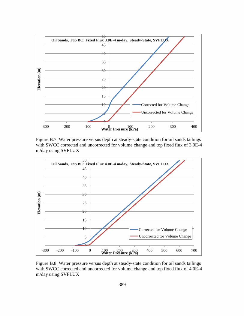
389
Figure B.7. Water pressure versus depth at steady-state condition for oil sands tailings
with SWCC corrected and uncorrected for volume change and top fixed flux of 3.0E-4
m/day using SVFLUX
Figure B.8. Water pressure versus depth at steady-state condition for oil sands tailings
with SWCC corrected and uncorrected for volume change and top fixed flux of 4.0E-4
m/day using SVFLUX
0
5
10
15
20
25
30
35
40
45
50
-300 -200 -100 0 100 200 300 400
Ele
va
tio
n (
m)
Water Pressure (kPa)
Oil Sands, Top BC: Fixed Flux 3.0E-4 m/day, Steady-State, SVFLUX
Corrected for Volume Change
Uncorrected for Volume Change
0
5
10
15
20
25
30
35
40
45
50
-300 -200 -100 0 100 200 300 400 500 600 700
Ele
va
tio
n (
m)
Water Pressure (kPa)
Oil Sands, Top BC: Fixed Flux 4.0E-4 m/day, Steady-State, SVFLUX
Corrected for Volume Change
Uncorrected for Volume Change
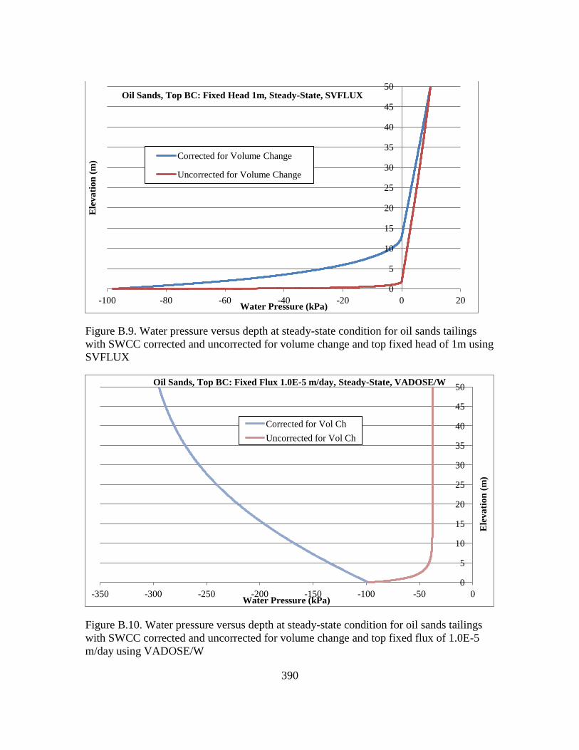
390
Figure B.9. Water pressure versus depth at steady-state condition for oil sands tailings
with SWCC corrected and uncorrected for volume change and top fixed head of 1m using
SVFLUX
Figure B.10. Water pressure versus depth at steady-state condition for oil sands tailings
with SWCC corrected and uncorrected for volume change and top fixed flux of 1.0E-5
m/day using VADOSE/W
0
5
10
15
20
25
30
35
40
45
50
-100 -80 -60 -40 -20 0 20
Ele
va
tio
n (
m)
Water Pressure (kPa)
Oil Sands, Top BC: Fixed Head 1m, Steady-State, SVFLUX
Corrected for Volume Change
Uncorrected for Volume Change
0
5
10
15
20
25
30
35
40
45
50
-350 -300 -250 -200 -150 -100 -50 0
Ele
va
tio
n (
m)
Water Pressure (kPa)
Oil Sands, Top BC: Fixed Flux 1.0E-5 m/day, Steady-State, VADOSE/W
Corrected for Vol Ch
Uncorrected for Vol Ch
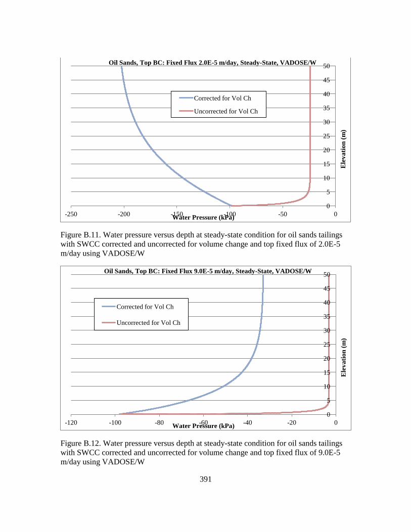
391
Figure B.11. Water pressure versus depth at steady-state condition for oil sands tailings
with SWCC corrected and uncorrected for volume change and top fixed flux of 2.0E-5
m/day using VADOSE/W
Figure B.12. Water pressure versus depth at steady-state condition for oil sands tailings
with SWCC corrected and uncorrected for volume change and top fixed flux of 9.0E-5
m/day using VADOSE/W
0
5
10
15
20
25
30
35
40
45
50
-250 -200 -150 -100 -50 0
Ele
va
tio
n (
m)
Water Pressure (kPa)
Oil Sands, Top BC: Fixed Flux 2.0E-5 m/day, Steady-State, VADOSE/W
Corrected for Vol Ch
Uncorrected for Vol Ch
0
5
10
15
20
25
30
35
40
45
50
-120 -100 -80 -60 -40 -20 0
Ele
va
tio
n (
m)
Water Pressure (kPa)
Oil Sands, Top BC: Fixed Flux 9.0E-5 m/day, Steady-State, VADOSE/W
Corrected for Vol Ch
Uncorrected for Vol Ch
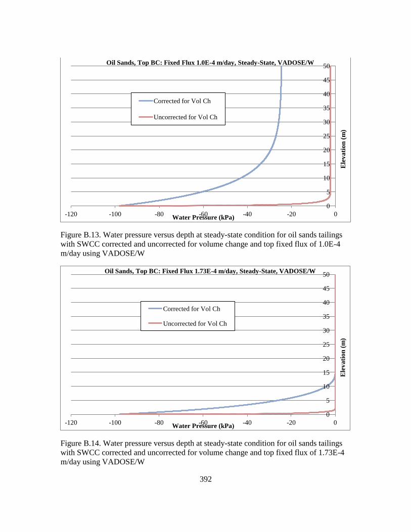
392
Figure B.13. Water pressure versus depth at steady-state condition for oil sands tailings
with SWCC corrected and uncorrected for volume change and top fixed flux of 1.0E-4
m/day using VADOSE/W
Figure B.14. Water pressure versus depth at steady-state condition for oil sands tailings
with SWCC corrected and uncorrected for volume change and top fixed flux of 1.73E-4
m/day using VADOSE/W
0
5
10
15
20
25
30
35
40
45
50
-120 -100 -80 -60 -40 -20 0
Ele
va
tio
n (
m)
Water Pressure (kPa)
Oil Sands, Top BC: Fixed Flux 1.0E-4 m/day, Steady-State, VADOSE/W
Corrected for Vol Ch
Uncorrected for Vol Ch
0
5
10
15
20
25
30
35
40
45
50
-120 -100 -80 -60 -40 -20 0
Ele
va
tio
n (
m)
Water Pressure (kPa)
Oil Sands, Top BC: Fixed Flux 1.73E-4 m/day, Steady-State, VADOSE/W
Corrected for Vol Ch
Uncorrected for Vol Ch
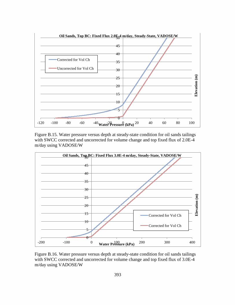
393
Figure B.15. Water pressure versus depth at steady-state condition for oil sands tailings
with SWCC corrected and uncorrected for volume change and top fixed flux of 2.0E-4
m/day using VADOSE/W
Figure B.16. Water pressure versus depth at steady-state condition for oil sands tailings
with SWCC corrected and uncorrected for volume change and top fixed flux of 3.0E-4
m/day using VADOSE/W
0
5
10
15
20
25
30
35
40
45
50
-120 -100 -80 -60 -40 -20 0 20 40 60 80 100
Ele
va
tio
n (
m)
Water Pressure (kPa)
Oil Sands, Top BC: Fixed Flux 2.0E-4 m/day, Steady-State, VADOSE/W
Corrected for Vol Ch
Uncorrected for Vol Ch
0
5
10
15
20
25
30
35
40
45
50
-200 -100 0 100 200 300 400
Ele
va
tio
n (
m)
Water Pressure (kPa)
Oil Sands, Top BC: Fixed Flux 3.0E-4 m/day, Steady-State, VADOSE/W
Corrected for Vol Ch
Corrected for Vol Ch
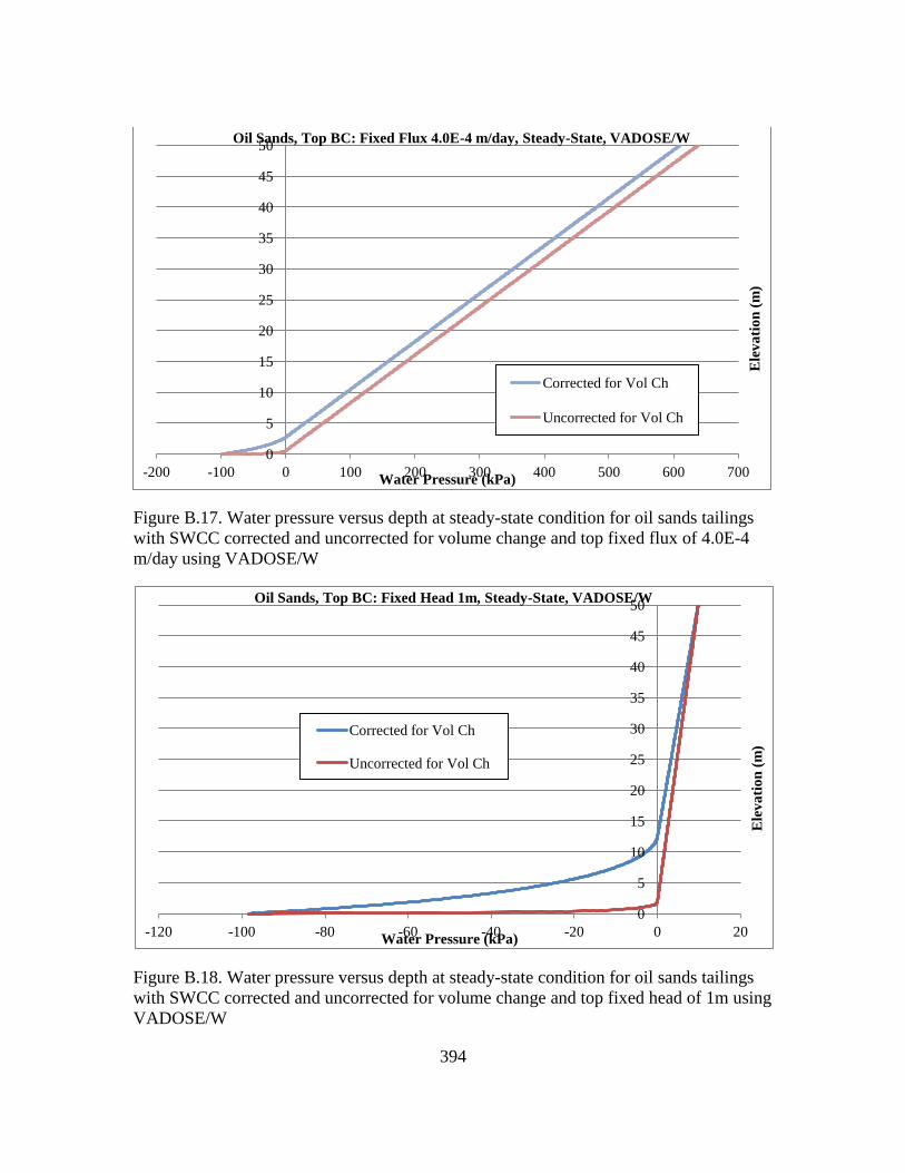
394
Figure B.17. Water pressure versus depth at steady-state condition for oil sands tailings
with SWCC corrected and uncorrected for volume change and top fixed flux of 4.0E-4
m/day using VADOSE/W
Figure B.18. Water pressure versus depth at steady-state condition for oil sands tailings
with SWCC corrected and uncorrected for volume change and top fixed head of 1m using
VADOSE/W
0
5
10
15
20
25
30
35
40
45
50
-200 -100 0 100 200 300 400 500 600 700
Ele
va
tio
n (
m)
Water Pressure (kPa)
Oil Sands, Top BC: Fixed Flux 4.0E-4 m/day, Steady-State, VADOSE/W
Corrected for Vol Ch
Uncorrected for Vol Ch
0
5
10
15
20
25
30
35
40
45
50
-120 -100 -80 -60 -40 -20 0 20
Ele
va
tio
n (
m)
Water Pressure (kPa)
Oil Sands, Top BC: Fixed Head 1m, Steady-State, VADOSE/W
Corrected for Vol Ch
Uncorrected for Vol Ch
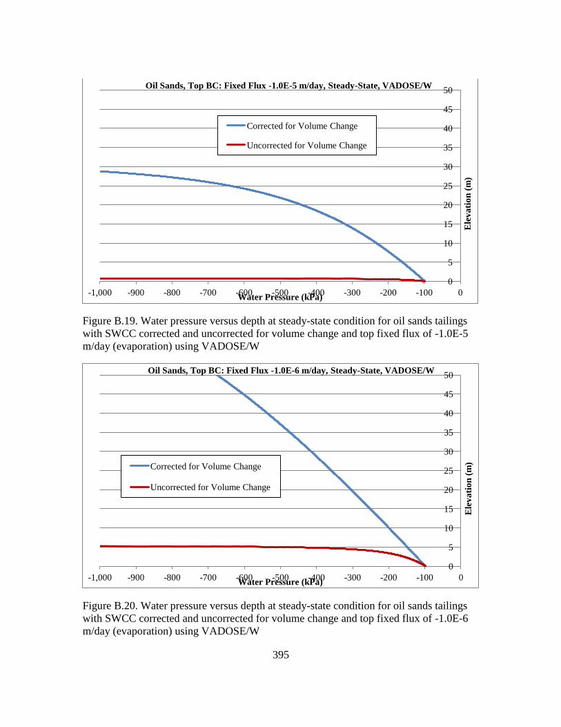
395
Figure B.19. Water pressure versus depth at steady-state condition for oil sands tailings
with SWCC corrected and uncorrected for volume change and top fixed flux of -1.0E-5
m/day (evaporation) using VADOSE/W
Figure B.20. Water pressure versus depth at steady-state condition for oil sands tailings
with SWCC corrected and uncorrected for volume change and top fixed flux of -1.0E-6
m/day (evaporation) using VADOSE/W
0
5
10
15
20
25
30
35
40
45
50
-1,000 -900 -800 -700 -600 -500 -400 -300 -200 -100 0
Ele
va
tio
n (
m)
Water Pressure (kPa)
Oil Sands, Top BC: Fixed Flux -1.0E-5 m/day, Steady-State, VADOSE/W
Corrected for Volume Change
Uncorrected for Volume Change
0
5
10
15
20
25
30
35
40
45
50
-1,000 -900 -800 -700 -600 -500 -400 -300 -200 -100 0
Ele
va
tio
n (
m)
Water Pressure (kPa)
Oil Sands, Top BC: Fixed Flux -1.0E-6 m/day, Steady-State, VADOSE/W
Corrected for Volume Change
Uncorrected for Volume Change
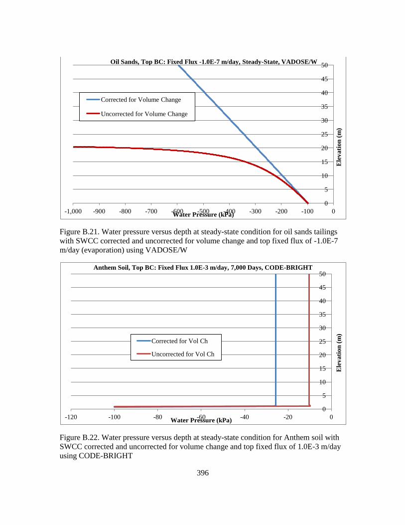
396
Figure B.21. Water pressure versus depth at steady-state condition for oil sands tailings
with SWCC corrected and uncorrected for volume change and top fixed flux of -1.0E-7
m/day (evaporation) using VADOSE/W
Figure B.22. Water pressure versus depth at steady-state condition for Anthem soil with
SWCC corrected and uncorrected for volume change and top fixed flux of 1.0E-3 m/day
using CODE-BRIGHT
0
5
10
15
20
25
30
35
40
45
50
-1,000 -900 -800 -700 -600 -500 -400 -300 -200 -100 0
Ele
va
tio
n (
m)
Water Pressure (kPa)
Oil Sands, Top BC: Fixed Flux -1.0E-7 m/day, Steady-State, VADOSE/W
Corrected for Volume Change
Uncorrected for Volume Change
0
5
10
15
20
25
30
35
40
45
50
-120 -100 -80 -60 -40 -20 0
Ele
va
tio
n (
m)
Water Pressure (kPa)
Anthem Soil, Top BC: Fixed Flux 1.0E-3 m/day, 7,000 Days, CODE-BRIGHT
Corrected for Vol Ch
Uncorrected for Vol Ch
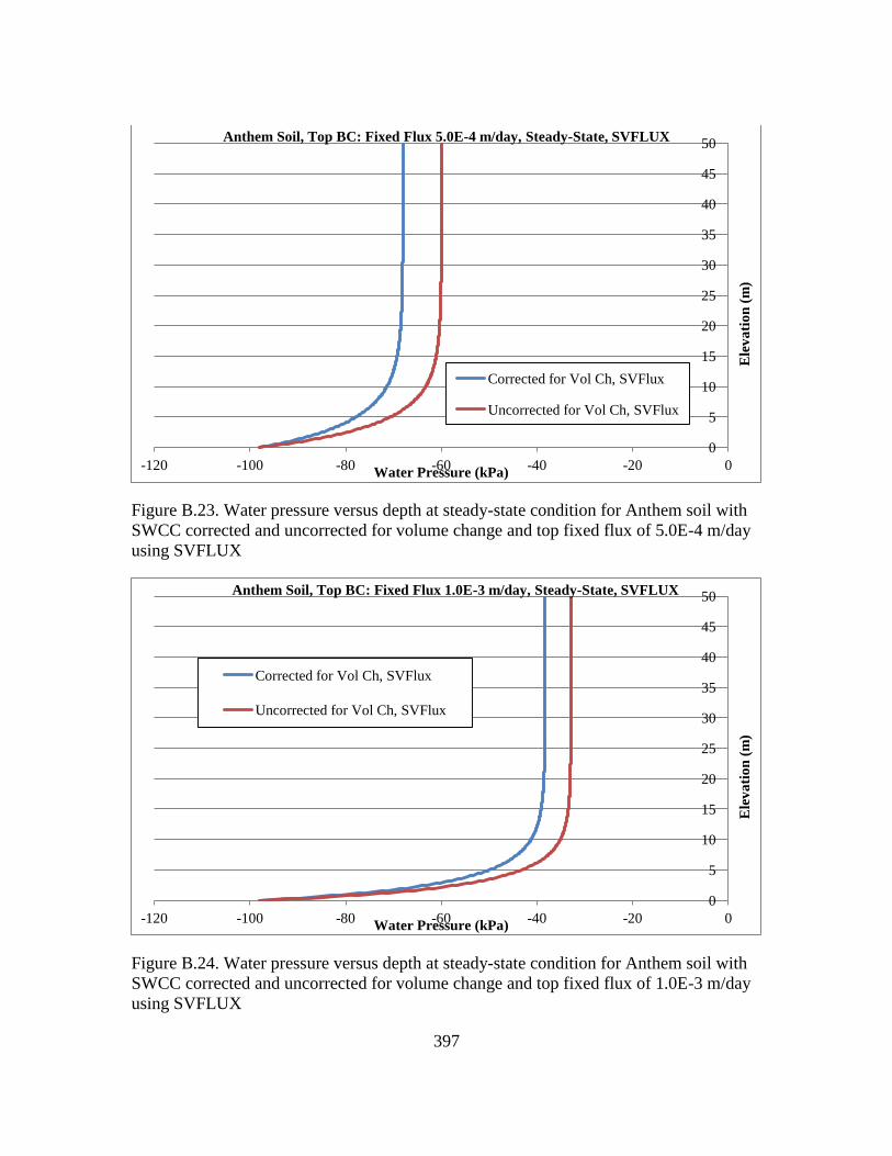
397
Figure B.23. Water pressure versus depth at steady-state condition for Anthem soil with
SWCC corrected and uncorrected for volume change and top fixed flux of 5.0E-4 m/day
using SVFLUX
Figure B.24. Water pressure versus depth at steady-state condition for Anthem soil with
SWCC corrected and uncorrected for volume change and top fixed flux of 1.0E-3 m/day
using SVFLUX
0
5
10
15
20
25
30
35
40
45
50
-120 -100 -80 -60 -40 -20 0
Ele
va
tio
n (
m)
Water Pressure (kPa)
Anthem Soil, Top BC: Fixed Flux 5.0E-4 m/day, Steady-State, SVFLUX
Corrected for Vol Ch, SVFlux
Uncorrected for Vol Ch, SVFlux
0
5
10
15
20
25
30
35
40
45
50
-120 -100 -80 -60 -40 -20 0
Ele
va
tio
n (
m)
Water Pressure (kPa)
Anthem Soil, Top BC: Fixed Flux 1.0E-3 m/day, Steady-State, SVFLUX
Corrected for Vol Ch, SVFlux
Uncorrected for Vol Ch, SVFlux
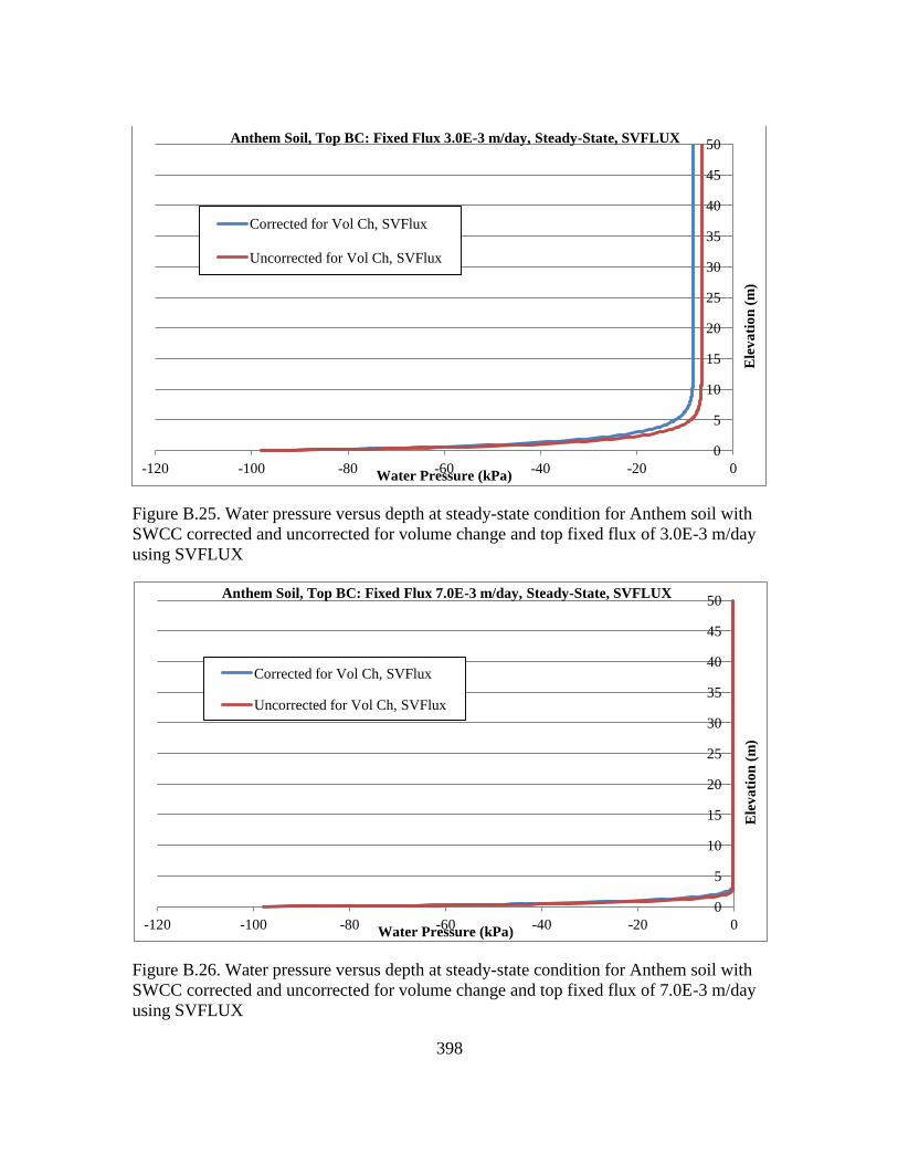
398
Figure B.25. Water pressure versus depth at steady-state condition for Anthem soil with
SWCC corrected and uncorrected for volume change and top fixed flux of 3.0E-3 m/day
using SVFLUX
Figure B.26. Water pressure versus depth at steady-state condition for Anthem soil with
SWCC corrected and uncorrected for volume change and top fixed flux of 7.0E-3 m/day
using SVFLUX
0
5
10
15
20
25
30
35
40
45
50
-120 -100 -80 -60 -40 -20 0
Ele
va
tio
n (
m)
Water Pressure (kPa)
Anthem Soil, Top BC: Fixed Flux 3.0E-3 m/day, Steady-State, SVFLUX
Corrected for Vol Ch, SVFlux
Uncorrected for Vol Ch, SVFlux
0
5
10
15
20
25
30
35
40
45
50
-120 -100 -80 -60 -40 -20 0
Ele
va
tio
n (
m)
Water Pressure (kPa)
Anthem Soil, Top BC: Fixed Flux 7.0E-3 m/day, Steady-State, SVFLUX
Corrected for Vol Ch, SVFlux
Uncorrected for Vol Ch, SVFlux
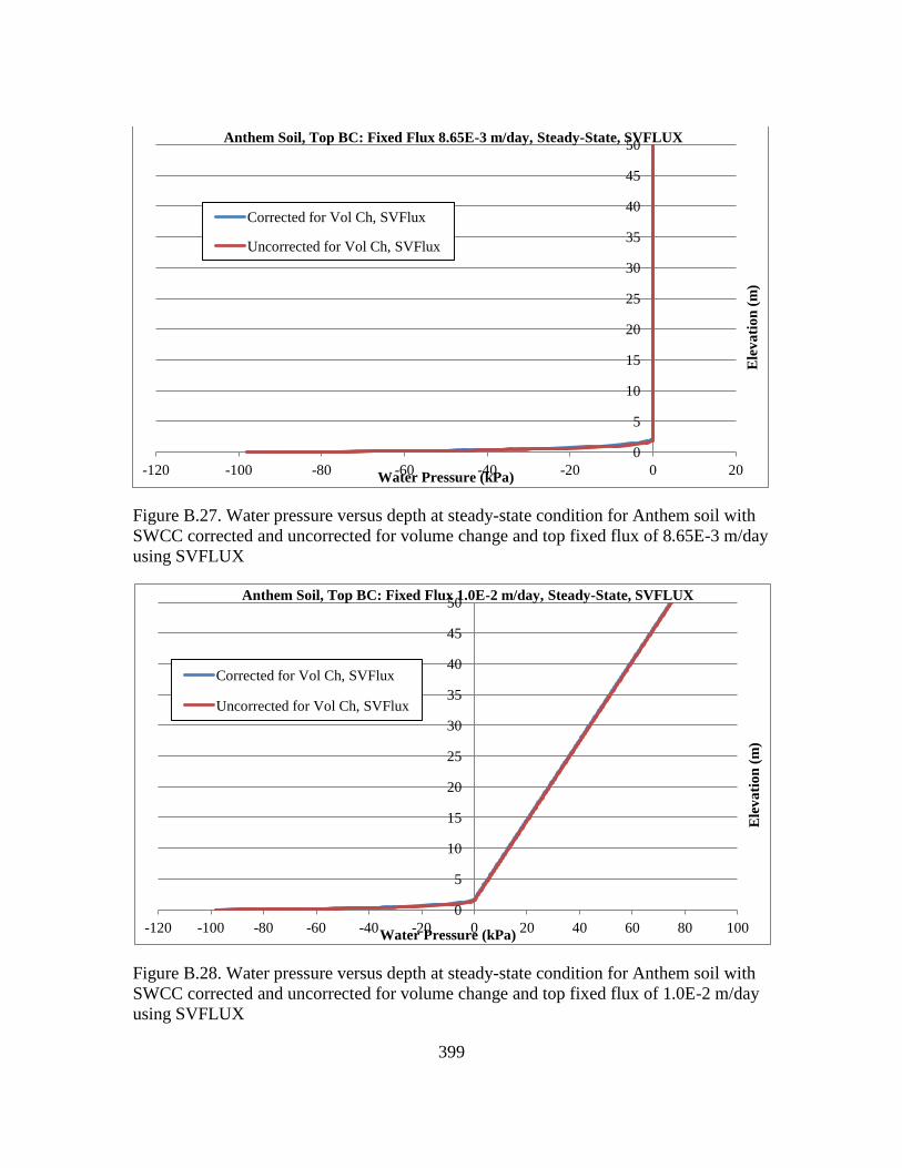
399
Figure B.27. Water pressure versus depth at steady-state condition for Anthem soil with
SWCC corrected and uncorrected for volume change and top fixed flux of 8.65E-3 m/day
using SVFLUX
Figure B.28. Water pressure versus depth at steady-state condition for Anthem soil with
SWCC corrected and uncorrected for volume change and top fixed flux of 1.0E-2 m/day
using SVFLUX
0
5
10
15
20
25
30
35
40
45
50
-120 -100 -80 -60 -40 -20 0 20
Ele
va
tio
n (
m)
Water Pressure (kPa)
Anthem Soil, Top BC: Fixed Flux 8.65E-3 m/day, Steady-State, SVFLUX
Corrected for Vol Ch, SVFlux
Uncorrected for Vol Ch, SVFlux
0
5
10
15
20
25
30
35
40
45
50
-120 -100 -80 -60 -40 -20 0 20 40 60 80 100
Ele
va
tio
n (
m)
Water Pressure (kPa)
Anthem Soil, Top BC: Fixed Flux 1.0E-2 m/day, Steady-State, SVFLUX
Corrected for Vol Ch, SVFlux
Uncorrected for Vol Ch, SVFlux
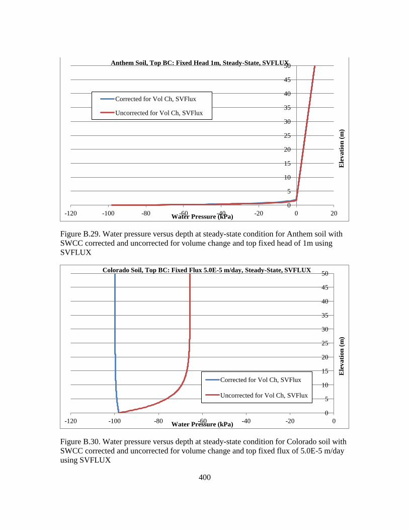
400
Figure B.29. Water pressure versus depth at steady-state condition for Anthem soil with
SWCC corrected and uncorrected for volume change and top fixed head of 1m using
SVFLUX
Figure B.30. Water pressure versus depth at steady-state condition for Colorado soil with
SWCC corrected and uncorrected for volume change and top fixed flux of 5.0E-5 m/day
using SVFLUX
0
5
10
15
20
25
30
35
40
45
50
-120 -100 -80 -60 -40 -20 0 20
Ele
va
tio
n (
m)
Water Pressure (kPa)
Anthem Soil, Top BC: Fixed Head 1m, Steady-State, SVFLUX
Corrected for Vol Ch, SVFlux
Uncorrected for Vol Ch, SVFlux
0
5
10
15
20
25
30
35
40
45
50
-120 -100 -80 -60 -40 -20 0
Ele
va
tio
n (
m)
Water Pressure (kPa)
Colorado Soil, Top BC: Fixed Flux 5.0E-5 m/day, Steady-State, SVFLUX
Corrected for Vol Ch, SVFlux
Uncorrected for Vol Ch, SVFlux
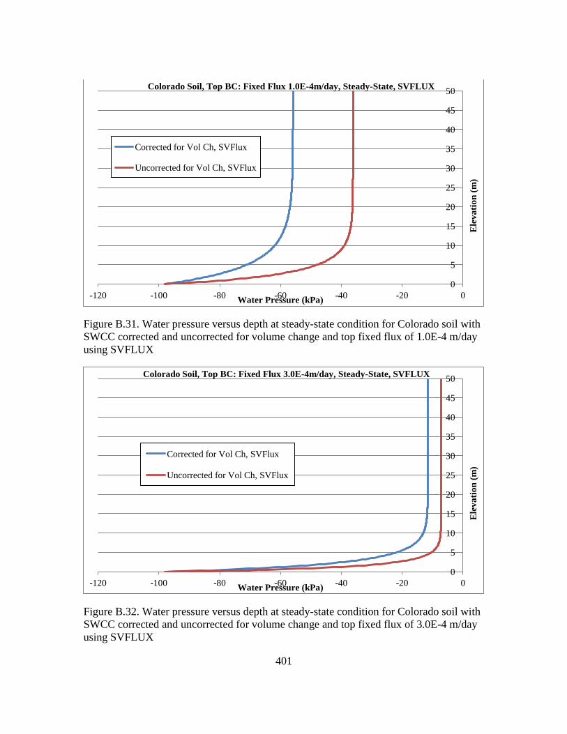
401
Figure B.31. Water pressure versus depth at steady-state condition for Colorado soil with
SWCC corrected and uncorrected for volume change and top fixed flux of 1.0E-4 m/day
using SVFLUX
Figure B.32. Water pressure versus depth at steady-state condition for Colorado soil with
SWCC corrected and uncorrected for volume change and top fixed flux of 3.0E-4 m/day
using SVFLUX
0
5
10
15
20
25
30
35
40
45
50
-120 -100 -80 -60 -40 -20 0
Ele
va
tio
n (
m)
Water Pressure (kPa)
Colorado Soil, Top BC: Fixed Flux 1.0E-4m/day, Steady-State, SVFLUX
Corrected for Vol Ch, SVFlux
Uncorrected for Vol Ch, SVFlux
0
5
10
15
20
25
30
35
40
45
50
-120 -100 -80 -60 -40 -20 0
Ele
va
tio
n (
m)
Water Pressure (kPa)
Colorado Soil, Top BC: Fixed Flux 3.0E-4m/day, Steady-State, SVFLUX
Corrected for Vol Ch, SVFlux
Uncorrected for Vol Ch, SVFlux
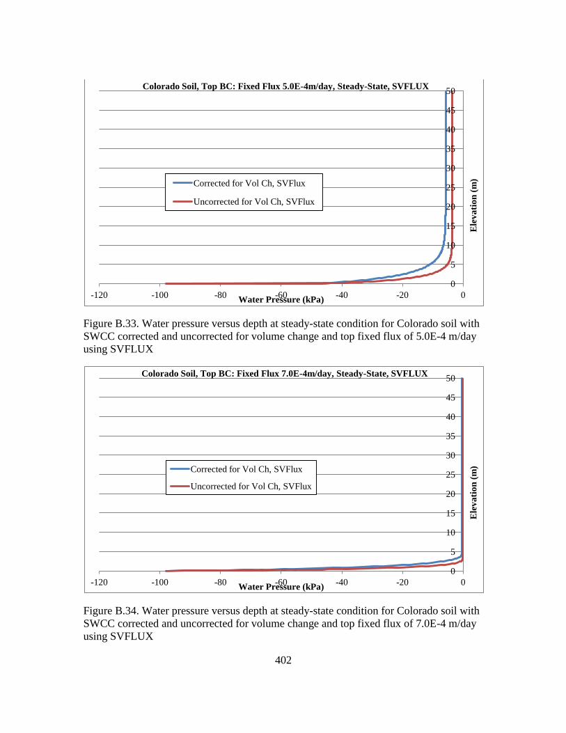
402
Figure B.33. Water pressure versus depth at steady-state condition for Colorado soil with
SWCC corrected and uncorrected for volume change and top fixed flux of 5.0E-4 m/day
using SVFLUX
Figure B.34. Water pressure versus depth at steady-state condition for Colorado soil with
SWCC corrected and uncorrected for volume change and top fixed flux of 7.0E-4 m/day
using SVFLUX
0
5
10
15
20
25
30
35
40
45
50
-120 -100 -80 -60 -40 -20 0
Ele
va
tio
n (
m)
Water Pressure (kPa)
Colorado Soil, Top BC: Fixed Flux 5.0E-4m/day, Steady-State, SVFLUX
Corrected for Vol Ch, SVFlux
Uncorrected for Vol Ch, SVFlux
0
5
10
15
20
25
30
35
40
45
50
-120 -100 -80 -60 -40 -20 0
Ele
va
tio
n (
m)
Water Pressure (kPa)
Colorado Soil, Top BC: Fixed Flux 7.0E-4m/day, Steady-State, SVFLUX
Corrected for Vol Ch, SVFlux
Uncorrected for Vol Ch, SVFlux
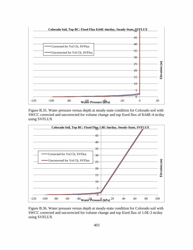
403
Figure B.35. Water pressure versus depth at steady-state condition for Colorado soil with
SWCC corrected and uncorrected for volume change and top fixed flux of 8.64E-4 m/day
using SVFLUX
Figure B.36. Water pressure versus depth at steady-state condition for Colorado soil with
SWCC corrected and uncorrected for volume change and top fixed flux of 1.0E-3 m/day
using SVFLUX
0
5
10
15
20
25
30
35
40
45
50
-120 -100 -80 -60 -40 -20 0 20
Ele
va
tio
n (
m)
Water Pressure (kPa)
Colorado Soil, Top BC: Fixed Flux 8.64E-4m/day, Steady-State, SVFLUX
Corrected for Vol Ch, SVFlux
Uncorrected for Vol Ch, SVFlux
0
5
10
15
20
25
30
35
40
45
50
-120 -100 -80 -60 -40 -20 0 20 40 60 80 100
Ele
va
tio
n (
m)
Water Pressure (kPa)
Colorado Soil, Top BC: Fixed Flux 1.0E-3m/day, Steady-State, SVFLUX
Corrected for Vol Ch, SVFlux
Uncorrected for Vol Ch, SVFlux
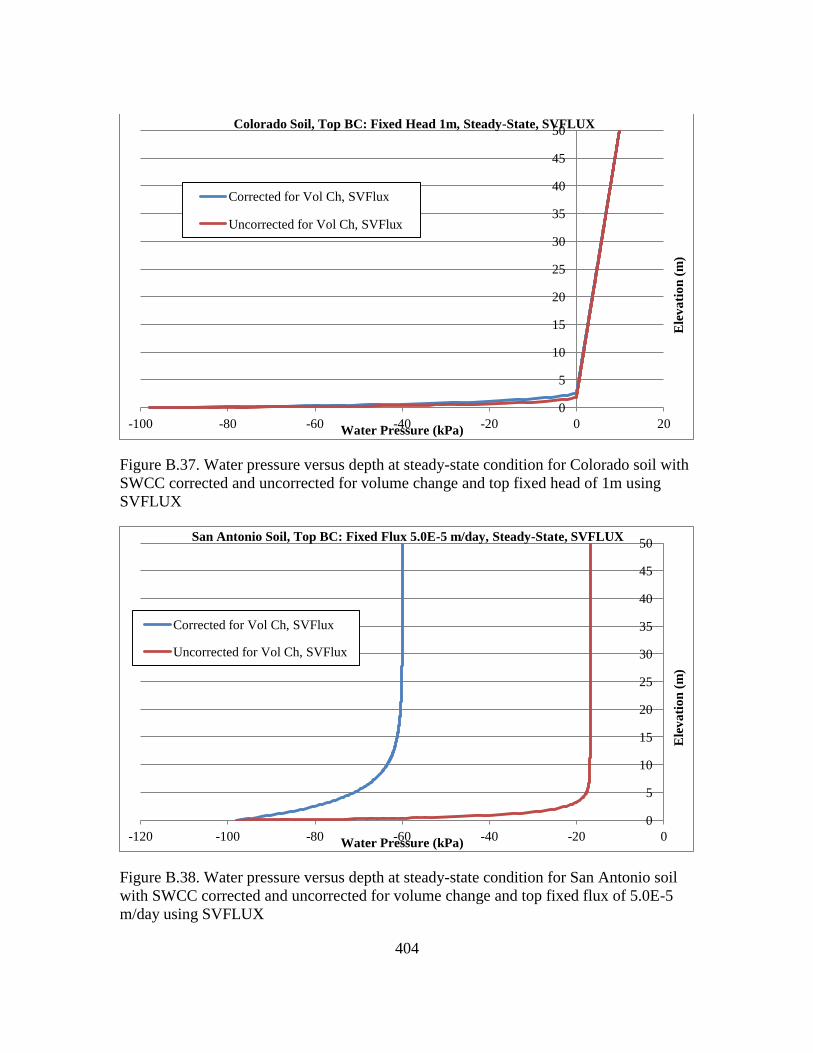
404
Figure B.37. Water pressure versus depth at steady-state condition for Colorado soil with
SWCC corrected and uncorrected for volume change and top fixed head of 1m using
SVFLUX
Figure B.38. Water pressure versus depth at steady-state condition for San Antonio soil
with SWCC corrected and uncorrected for volume change and top fixed flux of 5.0E-5
m/day using SVFLUX
0
5
10
15
20
25
30
35
40
45
50
-100 -80 -60 -40 -20 0 20
Ele
va
tio
n (
m)
Water Pressure (kPa)
Colorado Soil, Top BC: Fixed Head 1m, Steady-State, SVFLUX
Corrected for Vol Ch, SVFlux
Uncorrected for Vol Ch, SVFlux
0
5
10
15
20
25
30
35
40
45
50
-120 -100 -80 -60 -40 -20 0
Ele
va
tio
n (
m)
Water Pressure (kPa)
San Antonio Soil, Top BC: Fixed Flux 5.0E-5 m/day, Steady-State, SVFLUX
Corrected for Vol Ch, SVFlux
Uncorrected for Vol Ch, SVFlux
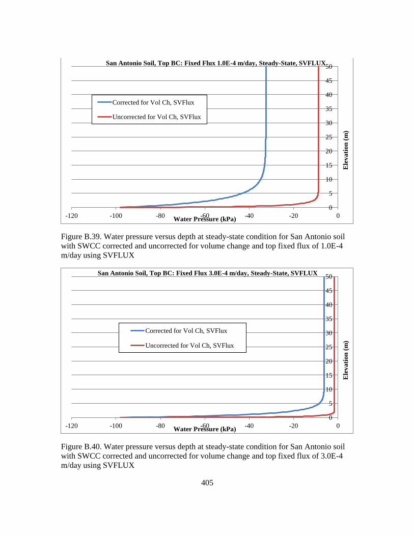
405
Figure B.39. Water pressure versus depth at steady-state condition for San Antonio soil
with SWCC corrected and uncorrected for volume change and top fixed flux of 1.0E-4
m/day using SVFLUX
Figure B.40. Water pressure versus depth at steady-state condition for San Antonio soil
with SWCC corrected and uncorrected for volume change and top fixed flux of 3.0E-4
m/day using SVFLUX
0
5
10
15
20
25
30
35
40
45
50
-120 -100 -80 -60 -40 -20 0
Ele
va
tio
n (
m)
Water Pressure (kPa)
San Antonio Soil, Top BC: Fixed Flux 1.0E-4 m/day, Steady-State, SVFLUX
Corrected for Vol Ch, SVFlux
Uncorrected for Vol Ch, SVFlux
0
5
10
15
20
25
30
35
40
45
50
-120 -100 -80 -60 -40 -20 0
Ele
va
tio
n (
m)
Water Pressure (kPa)
San Antonio Soil, Top BC: Fixed Flux 3.0E-4 m/day, Steady-State, SVFLUX
Corrected for Vol Ch, SVFlux
Uncorrected for Vol Ch, SVFlux
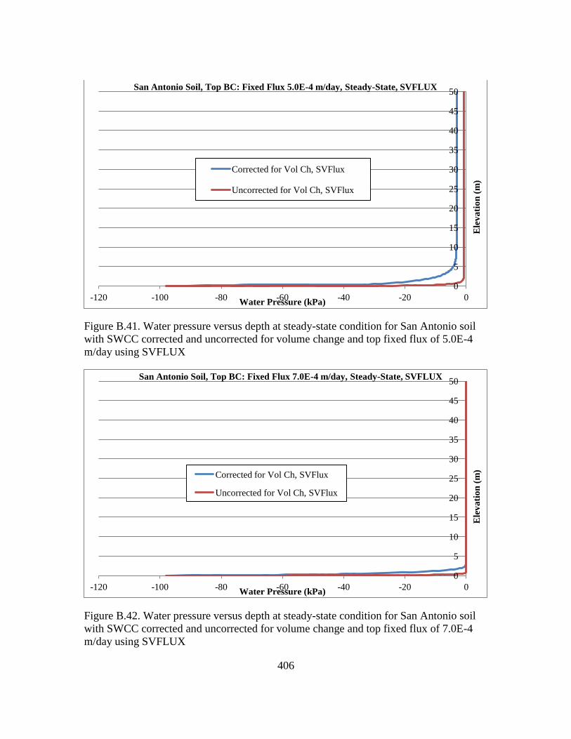
406
Figure B.41. Water pressure versus depth at steady-state condition for San Antonio soil
with SWCC corrected and uncorrected for volume change and top fixed flux of 5.0E-4
m/day using SVFLUX
Figure B.42. Water pressure versus depth at steady-state condition for San Antonio soil
with SWCC corrected and uncorrected for volume change and top fixed flux of 7.0E-4
m/day using SVFLUX
0
5
10
15
20
25
30
35
40
45
50
-120 -100 -80 -60 -40 -20 0
Ele
va
tio
n (
m)
Water Pressure (kPa)
San Antonio Soil, Top BC: Fixed Flux 5.0E-4 m/day, Steady-State, SVFLUX
Corrected for Vol Ch, SVFlux
Uncorrected for Vol Ch, SVFlux
0
5
10
15
20
25
30
35
40
45
50
-120 -100 -80 -60 -40 -20 0
Ele
va
tio
n (
m)
Water Pressure (kPa)
San Antonio Soil, Top BC: Fixed Flux 7.0E-4 m/day, Steady-State, SVFLUX
Corrected for Vol Ch, SVFlux
Uncorrected for Vol Ch, SVFlux
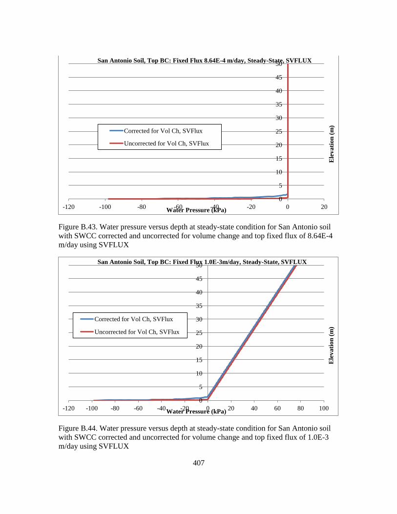
407
Figure B.43. Water pressure versus depth at steady-state condition for San Antonio soil
with SWCC corrected and uncorrected for volume change and top fixed flux of 8.64E-4
m/day using SVFLUX
Figure B.44. Water pressure versus depth at steady-state condition for San Antonio soil
with SWCC corrected and uncorrected for volume change and top fixed flux of 1.0E-3
m/day using SVFLUX
0
5
10
15
20
25
30
35
40
45
50
-120 -100 -80 -60 -40 -20 0 20
Ele
va
tio
n (
m)
Water Pressure (kPa)
San Antonio Soil, Top BC: Fixed Flux 8.64E-4 m/day, Steady-State, SVFLUX
Corrected for Vol Ch, SVFlux
Uncorrected for Vol Ch, SVFlux
0
5
10
15
20
25
30
35
40
45
50
-120 -100 -80 -60 -40 -20 0 20 40 60 80 100
Ele
va
tio
n (
m)
Water Pressure (kPa)
San Antonio Soil, Top BC: Fixed Flux 1.0E-3m/day, Steady-State, SVFLUX
Corrected for Vol Ch, SVFlux
Uncorrected for Vol Ch, SVFlux
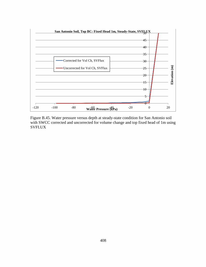
408
Figure B.45. Water pressure versus depth at steady-state condition for San Antonio soil
with SWCC corrected and uncorrected for volume change and top fixed head of 1m using
SVFLUX
0
5
10
15
20
25
30
35
40
45
50
-120 -100 -80 -60 -40 -20 0 20
Ele
va
tio
n (
m)
Water Pressure (kPa)
San Antonio Soil, Top BC: Fixed Head 1m, Steady-State, SVFLUX
Corrected for Vol Ch, SVFlux
Uncorrected for Vol Ch, SVFlux


![Chapter 3 PROBATE PROCEEDINGS - lexisone.com · § 3.21 Obtaining Letters of Administration, c.t.a. [1] Determining If Letters of Administration c.t.a. Are Appropriate [2] Determining](https://img.pdfslide.us/doc/110x75/5fb4d6976a167266956f579b/chapter-3-probate-proceedings-321-obtaining-letters-of-administration-cta.jpg)