Stephen Heron

GEO 327G Project

Volcanic Hazards of Mount Adams, Washington

Fall 2011

Stephen Heron

Stephen Heron

Volcanic Hazards of Mount Adams

Introduction:

The Cascades is a chain of mountains extending over much of western North America. It contains both non-volcanic and volcanic mountains. The “High Cascades”, which run from mid-Washington to northern California, is the part of the range that is made up of predominately volcanic mountains. The High Cascades include volcanoes such as Mount Rainier, Mount Hood, Mount St. Helens, and Mount Adams. Mount Adams is the second largest mountain in Washington State. It has not erupted in 1400 years, but is not yet considered extinct. What if it were to erupt?

Problem:

Volcanoes can be quite dangerous to people in surrounding areas. There are two main types of hazards involved. The first is flow hazards, such as lahars, lava flows, pyroclastic flows, and debris flows. Lahars are fast flows that occur when pyroclastic material combines with a lot of water. Lava flows are slow, but widespread traveling molten material. Pyroclastic flows are fast moving volcanic material. Debris flow is fast moving material. Each of these can be triggered by a volcano. The other type of hazard is tephra fall. Tephra is pyroclastic material launched out from the volcano (like ash or bombs). They can affect a much bigger area. I plan on using GIS to find out the approximate extent of damage of a volcanic eruption at Mount Adams by interpreting where conduits for flow hazards are. I will find out how many people in Washington are affected and the area of effect for each hazard. Finally, I will compare the interpreted conduits of flow hazards to USGS data.

1. Data Collection

Data for this project comes from three sources.

http://seamless.usgs.gov/website/seamless/viewer.htm The National Map Seamless Server (Fig 1.1). This program allows the user to highlight an area of the earth and select desired available data for that area. Zooming to Mount Adams allows the user to select the things like land cover, geology, bathymetry, and a whole lot more for the area. For this project, we will use a

-1/3 arc-second DEM (10 meters)

-Streams shapefile to determine lahar channels

-Roads for local reference

-Cities to determine location and numbers of affected people

-Counties for local reference

-Water bodies to determine lakes and rivers affected.

Stephen Heron

Fig 1.1: The National Map Seamless Server

http://vulcan.wr.usgs.gov/Volcanoes/Adams/framework.html The United States Geological Survey. The website contains a large amount of data on Mount Adams. Information about its volcanic hazards can be found here. It is given in a compressed .gz format, which must be preprocessed. This data will be used to compare to the techniques used in the project.

http://pubs.usgs.gov/of/1995/0492/report.pdf “Volcano Hazards in the Mount Adams Region, Washington” by William E. Scott et al. This isn’t digital data, but rather a paper that I referred to as a source for the numbers I will use later in the project for lava flows, pyroclastic flows, lahars, etc.

Stephen Heron

2. Data Preprocessing

The data gathered needed to be made into a useful format for ArcGIS. Files collected from the National Map Seamless Sever were zipped and named with incoherent numbers, identifiable only by the XML metadata that came along with it. After extracting all the files from their compressed, zipped form, rename the files to something you could more easily identify (Fig 2.1).

Fig 2.1: ArcCatalog showing renamed seamless data and useable metadata

Stephen Heron

The data collected from USGS was in the .gz format. To make this useable, I took the data to my home computer and downloaded a program called 7zip, which I used to extract the files into a .e00 format. Then I brought them back to a computer with ArcGIS to convert them into useable data. Go to ArcToolbox and select Coverage Tools > To Conversion > To Coverage > Import From Interchange File (Fig 2.2). This converts the .e00 file into ArcGIS compatible data.

Fig 2.2: Converting .e00 into ArcGIS compatible data.

Stephen Heron

The data from this conversion is in the wrong coordinate system and the wrong projection. To remedy this, first convert the coverage to a shapefile. Go to Conversion Tools > To Shapefile > Feature Class To Shapefile (multiple)(Fig 2.3).

Fig 2.3: Converting coverages to shapefiles.

Stephen Heron

Now, go to Data Management Tools > Projections and Transformations > Feature > Project and choose GCS_North_American_1983 (Fig 2.4). This puts the shapefile into the same coordinate system as the shapefiles gathered from the National Map Seamless Server. Repeat until all shapefiles are in the correct coordinate system.

Fig 2.4: Choosing the correct coordinate system for the new shapefiles.

Stephen Heron

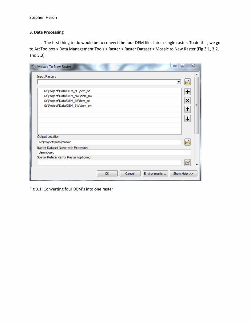
3. Data Processing

The first thing to do would be to convert the four DEM files into a single raster. To do this, we go to ArcToolbox > Data Management Tools > Raster > Raster Dataset > Mosaic to New Raster (Fig 3.1, 3.2, and 3.3).

Fig 3.1: Converting four DEM’s into one raster

Stephen Heron

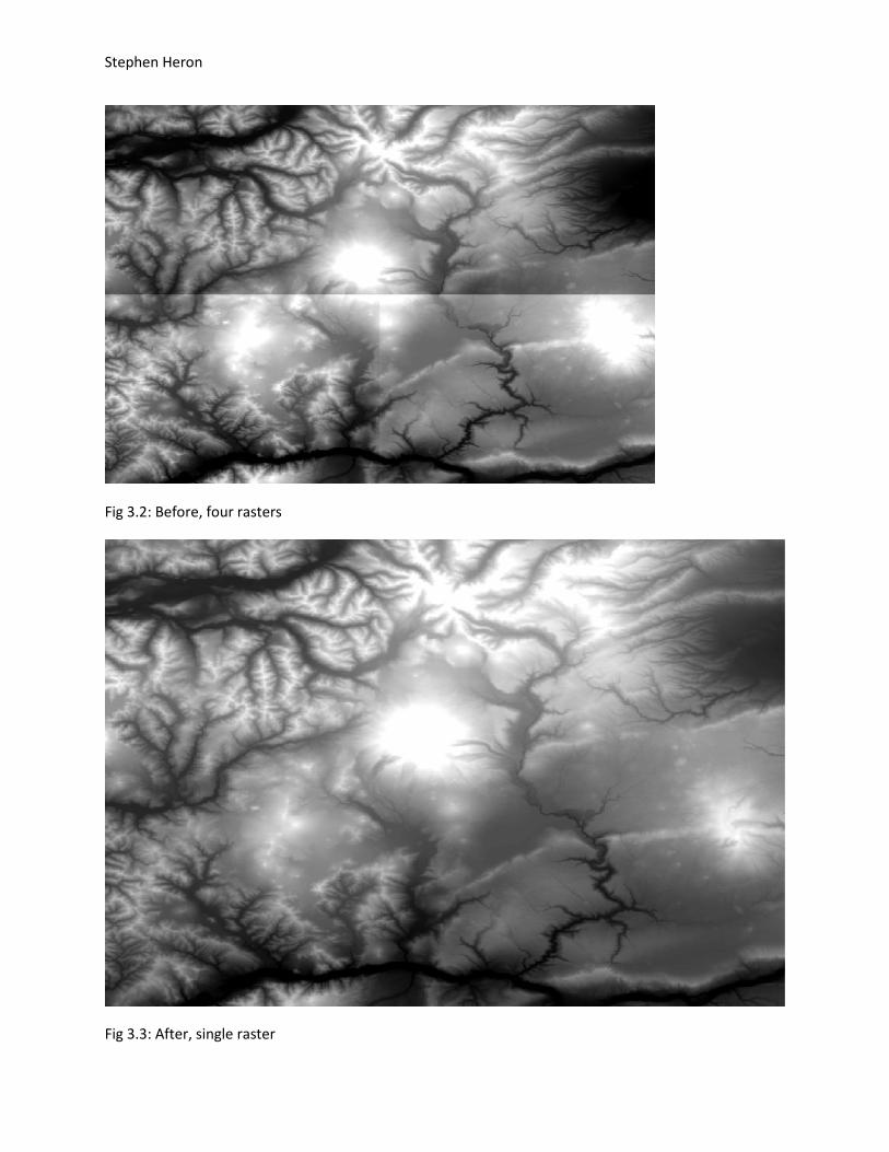
Fig 3.2: Before, four rasters

Fig 3.3: After, single raster

Stephen Heron

Before we can see the larger rivers properly, we must use the water bodies shapefile to make the more visible. Currently, the larger Columbia River is symbolized by two streams instead of a whole river. Using the attribute table of the water bodies diagram (3.4), select all of the Columbia River. Then right click the water bodies layer, go to selection, and click “Create Layer From Selected Features.” This gives you a layer for the Columbia River.

Fig 3.4: This selection selects the Columbia River which is used to create its own layer

The above step is repeated for other bodies of water that are too large to be represented by a line.

Stephen Heron

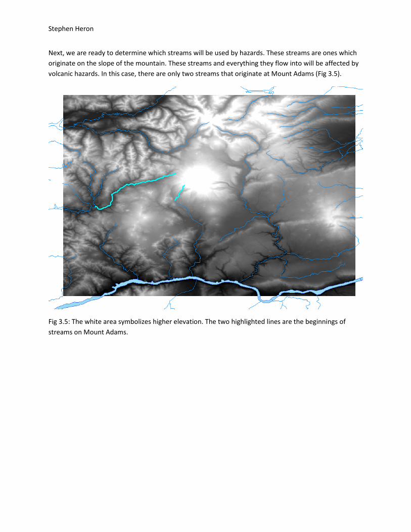
Next, we are ready to determine which streams will be used by hazards. These streams are ones which originate on the slope of the mountain. These streams and everything they flow into will be affected by volcanic hazards. In this case, there are only two streams that originate at Mount Adams (Fig 3.5).

Fig 3.5: The white area symbolizes higher elevation. The two highlighted lines are the beginnings of streams on Mount Adams.

Stephen Heron

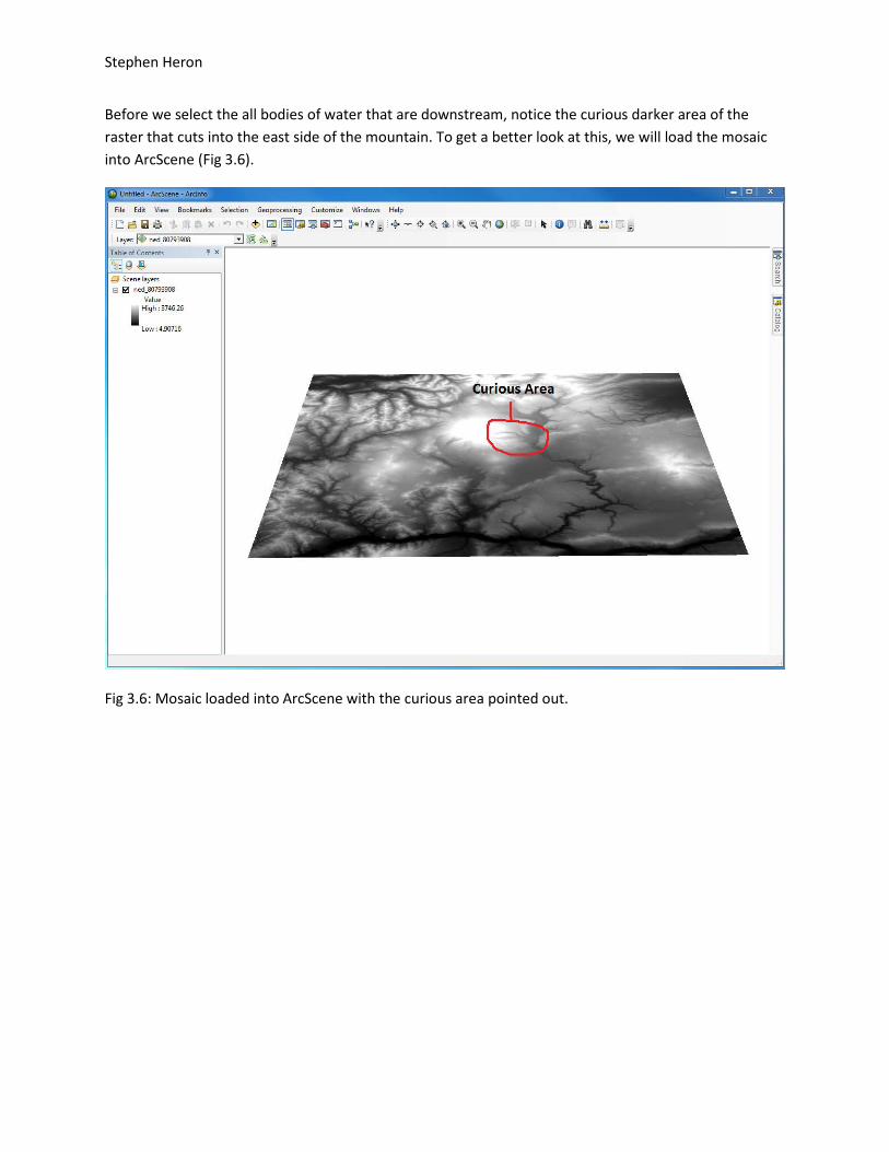
Before we select the all bodies of water that are downstream, notice the curious darker area of the raster that cuts into the east side of the mountain. To get a better look at this, we will load the mosaic into ArcScene (Fig 3.6).

Fig 3.6: Mosaic loaded into ArcScene with the curious area pointed out.

Stephen Heron

Then we will go to the mosaic’s properties and select “Floating on a custom surface” from the “Base Heights” tab. Change the factor to convert layer elevation values to scene units to .000009 (.000009 decimal degrees per meter). We then change the color to something more easily seen and the vertical exaggeration to 5 times normal (Fig 3.7). From this picture we can clearly see that the curious area is a deep valley that empties into a river. These can be used as conduits as well.

Fig 3.7: The “curious” area turned out to be two deep valleys that led to a river.

Stephen Heron

To use these newly found valleys as data, we need to digitize a polygon for them. Go to ArcCatalog and created a personal geodatabase, a feature dataset, and finally a line feature class for the valleys. Load this shapefile into ArcMap and start editing from the Editor toolbar. From there, select the line tool and click points to create lines for the valleys (Fig 3.8).

Fig 3.8: Valleys are digitized as lines.

We are only to use rivers that are downstream in our map. Excess will be cut out. We need to select all of the bodies of water downstream from the uphill streams. However, the Columbia River layer highlights areas that are upstream from where hazards could potentially make contact (Fig 3.9).

Fig 3.9: More of the Columbia River is selected than needed.

Stephen Heron

To fix this, we start editing from the editing toolbar. Select the “Cut Polygons Tool” icon and choose two vertices to split the polygon between. This results in two polygons where one used to be (Fig 3.10). Repeat this step for the river that meets the valleys conduit using instead the “Cut Lines Tool”.

Fig 3.10: The polygon that is downstream is now selectable separately from the upstream part.

Make the polygons that include the Columbia River and the three lake polygons that are downstream into one layer file by going to Geoprocessing > Union.

Stephen Heron

Make the valleys and the streams that will be used into a single layer called “Conduits”. This is done with Geoprocessing > Merge (Fig 3.11).

Fig 3.11: The conduits (in brown) and the water bodies (in blue).

Now we are ready to make buffers for the different hazards. In order to make a buffer on a line polygon, a width and distance is required. Using the Scott et al paper, we can approximate or assign values we need for the four flow based hazards (Table 3.1).

Width of Small (km) Width of Large (km) Distance of Small (km)

Distance of Large (km)

Debris Flow .1* N/A 6 N/A Pyroclastic Flow .2* .3* 10 15

Lahar N/A ~1 N/A 55 Lava Flow ~.4 ~.8 20 50 Table 3.1: ~Denotes values that were approximated from data given in the Scott et al paper. *Denotes values that were necessary, but unknown, so approximate values were assigned. Unmarked denotes data that was given in the Scott et al paper.

Stephen Heron

Go to Analysis Tools > Proximity > Buffer to create a buffer for the hazards (Fig 3.12). Repeat this for all hazards. We are using the width for the linear unit. Enter half of the width because the linear unit goes to both sides, giving it its full width value.

Fig 3.12: Creating a buffer for the large lahars.

Stephen Heron

This will give you buffers that run the whole length of the polygon (3.13). They are bunched together, but we will separate them later.

3.13: Buffered conduits.

Stephen Heron

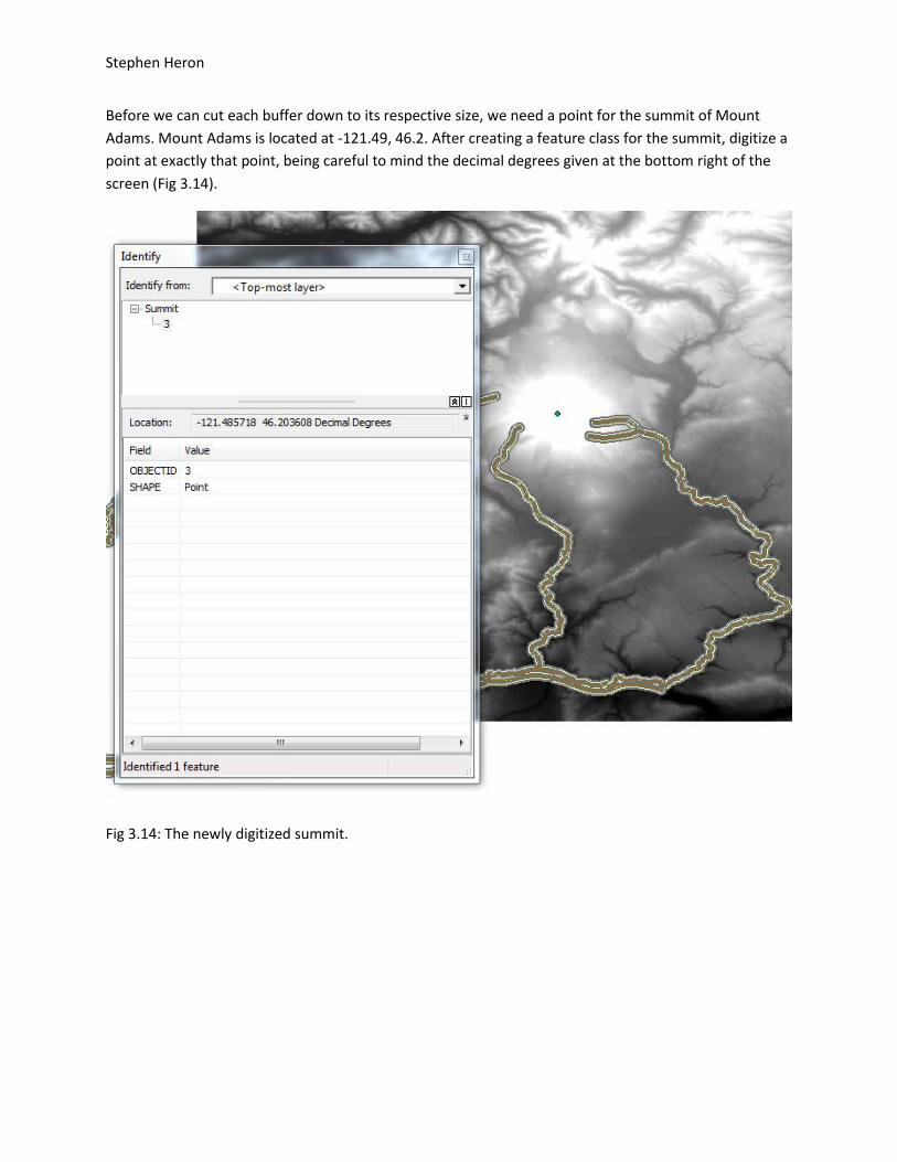
Before we can cut each buffer down to its respective size, we need a point for the summit of Mount Adams. Mount Adams is located at -121.49, 46.2. After creating a feature class for the summit, digitize a point at exactly that point, being careful to mind the decimal degrees given at the bottom right of the screen (Fig 3.14).

Fig 3.14: The newly digitized summit.

Stephen Heron

Now we need to clip the hazards to their respective lengths. To do this, create six buffers, using the summit as the input feature and the distance as the linear unit (Fig 3.15).

Fig 3.15: Creating a new buffer that the original will clip to.

Next, we will clip the original buffer to the new buffer (Fig 3.16). This will show the full width and distance of the hazard.

3.16: Clipping the new buffer to the original.

Stephen Heron

Repeat this for every hazard. Fig 3.17 is the result.

Fig 3.17: Clipped hazards.

Stephen Heron

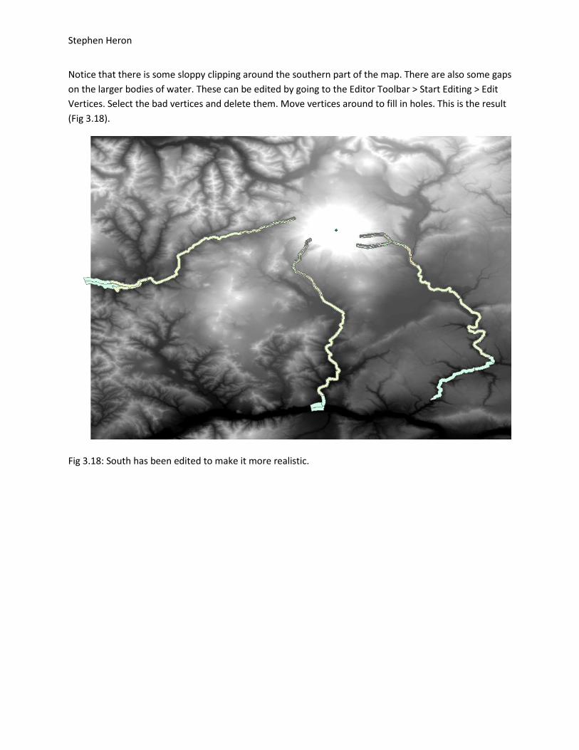
Notice that there is some sloppy clipping around the southern part of the map. There are also some gaps on the larger bodies of water. These can be edited by going to the Editor Toolbar > Start Editing > Edit Vertices. Select the bad vertices and delete them. Move vertices around to fill in holes. This is the result (Fig 3.18).

Fig 3.18: South has been edited to make it more realistic.

Stephen Heron

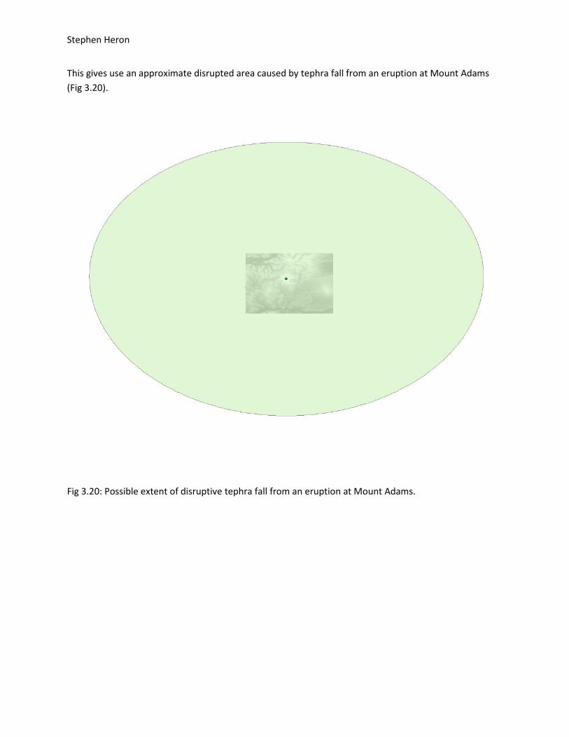
Now for tephra fragments! According to the Scott et al paper, ash was disruptive (defined as negatively affected transportation and business) as far as Spokane, Washington for the 1980 Mount St. Helens eruption (.5-8cm of ash). We can use this to approximate how far Mount Adams will be disruptive. Spokane is ~250 miles from the summit of Mount Adams. We can create a ring buffer symbolize the area affected. Go to Analysis Tools > Proximity > Buffer and input the summit as the input and 250 kilometers as the distance (Fig 3.19).

Fig 3.19: Tephra buffer.

Stephen Heron

This gives use an approximate disrupted area caused by tephra fall from an eruption at Mount Adams (Fig 3.20).

Fig 3.20: Possible extent of disruptive tephra fall from an eruption at Mount Adams.

Stephen Heron

4. Data Presentation

Now, we will examine the effects of flow hazards, followed by tephra fall hazards.

Lahars

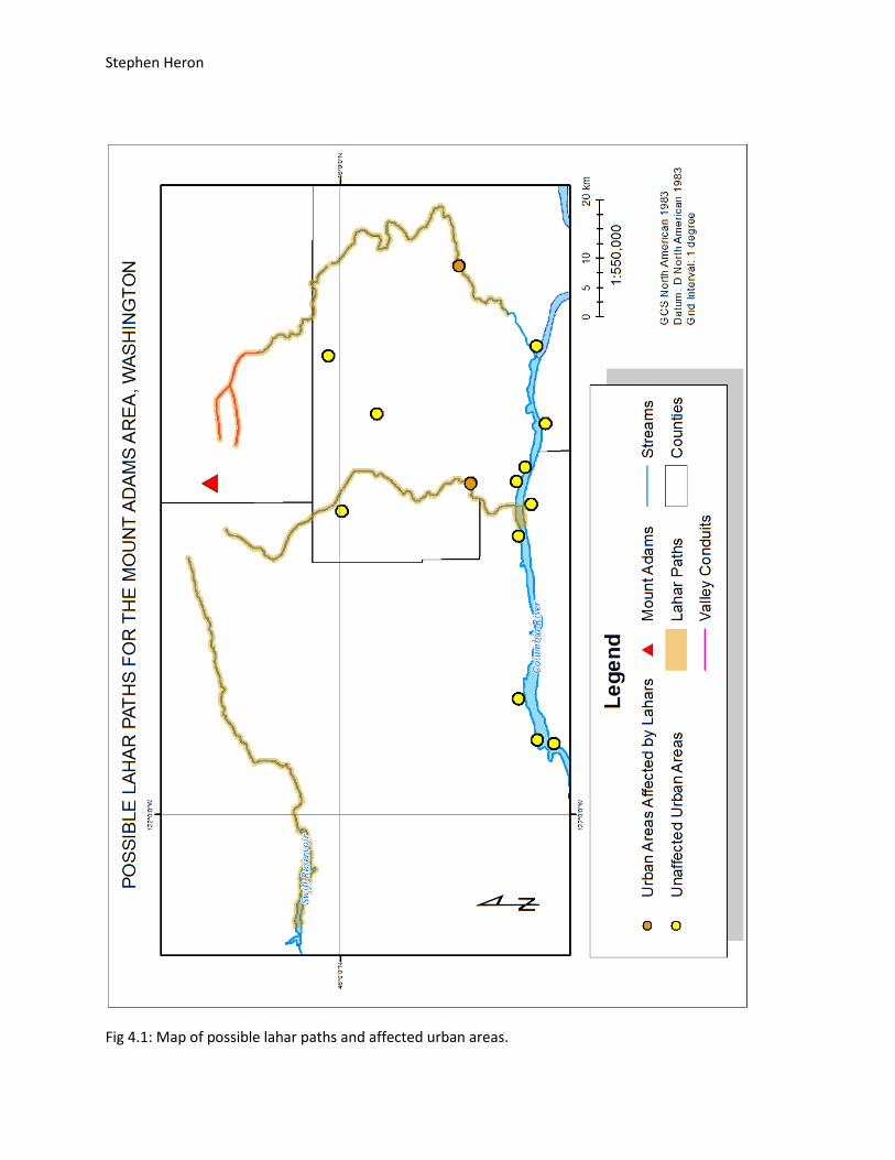
First, we will look at lahars. After making a map showing only the lahars and the cities they affect, use “Select By Location” to choose all cities that cross paths with the lahar. Create a layer for the selected cities. There are only two (Fig 4.1).

The towns affected are Klickitat and Husum. This is found by opening the attribute table for the affected urban areas layer (Fig 4.2).

Fig 4.2: Affected towns.

The affected bodies of water can be found with the same method. They are Swift Reservoir, Cascade Creek, Klickitat River, Lewis River, White Salmon River, and Columbia River.

We will examine the populations later.

Lava Flows

By enhancing our extent, and swapping out the Lahar Paths buffer for the large and small lava flow buffers, we can examine how lava flows affect the area. Select by Location again to find that only one urban area, Husum, is affected (Fig 4.3). It is affected only by the large lava flow.

The affected bodies of water are Swift Reservoir, Cascade Creek, Klickitat River, Lewis River, and White Salmon River.

Debris and Pyroclastic Flows

By further enhancing our extent, and swapping out the lava flow buffers for the small debris flow and the small and large pyroclastic flow buffers. The resulting map shows us that there is no urban area affect by debris or pyroclastic flows (4.4). The affected bodies of water are Cascade Creek, Lewis River, and White Salmon River.

Stephen Heron

Fig 4.1: Map of possible lahar paths and affected urban areas.

Stephen Heron

Fig 4.3: Map of possible lava flow paths and the affected urban area.

Stephen Heron

Fig 4.4: Map of possible pyroclastic and debris flow paths.

Stephen Heron

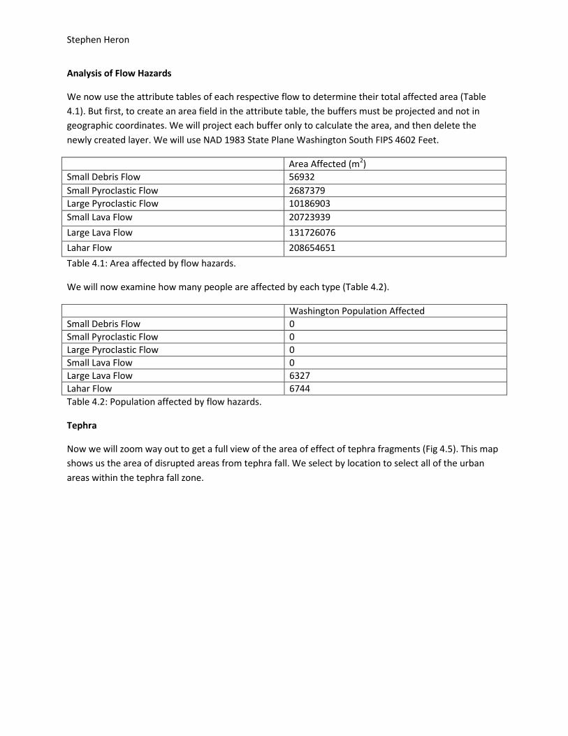
Analysis of Flow Hazards

We now use the attribute tables of each respective flow to determine their total affected area (Table 4.1). But first, to create an area field in the attribute table, the buffers must be projected and not in geographic coordinates. We will project each buffer only to calculate the area, and then delete the newly created layer. We will use NAD 1983 State Plane Washington South FIPS 4602 Feet.

Area Affected (m2) Small Debris Flow 56932 Small Pyroclastic Flow 2687379 Large Pyroclastic Flow 10186903 Small Lava Flow 20723939 Large Lava Flow 131726076 Lahar Flow 208654651 Table 4.1: Area affected by flow hazards.

We will now examine how many people are affected by each type (Table 4.2).

Washington Population Affected Small Debris Flow 0 Small Pyroclastic Flow 0 Large Pyroclastic Flow 0 Small Lava Flow 0 Large Lava Flow 6327 Lahar Flow 6744 Table 4.2: Population affected by flow hazards.

Tephra

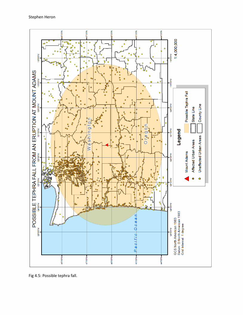
Now we will zoom way out to get a full view of the area of effect of tephra fragments (Fig 4.5). This map shows us the area of disrupted areas from tephra fall. We select by location to select all of the urban areas within the tephra fall zone.

Stephen Heron

Fig 4.5: Possible tephra fall.

Stephen Heron

Tephra Analysis

Now we will find the area and the population affected, just as above with flow hazards (Table 4.3).

Area Affected (km2) Washington Population Affected Tephra 196374 4064574 Table 4.3: Tephra affected area and population.

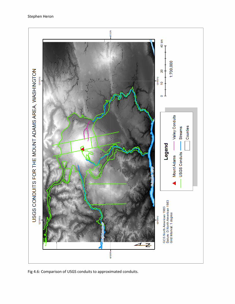
Comparison to USGS Data

USGS data was very limited for the Mount Adams area. The only useable data was a line data file showing possible conduits (Fig 4.6). This can be compared to the conduits I used. The DEM was added in to show how the conduits compare to the mountain’s features.

The map shows using the same conduits that I use. Additionally, it shows a conduit system on the northwest face of the mountain. It also shows an additional channel that feeds into the conduit I used that went south.

These additions to my data would have increased the total area affected significantly. It also would have increased the population affected, as seen by the city crossing the USGS data on the map.

Stephen Heron

Fig 4.6: Comparison of USGS conduits to approximated conduits.

Stephen Heron

5. Conclusion

Mount Adams, like its fellow volcanic Cascades, poses a serious threat to the Mount Adams area. Debris flows, pyroclastic flows, lava flows, and lahars are very dangerous. While lahars and large lava flows have the potential to destroy towns, the others will severely alter the landscape around them and anything nearby over the widespread area that they affect. Tephra fragments in Washington can be very disruptive over a much larger area than flow hazards. However, its damage is significantly less severe. Blocking the sun and disrupting transportation, among other things, makes a Mount Adams eruption very undesired.

When comparing raw data for flow hazards, lahars were the most widespread, and therefore dangerous. They were followed by large and small lava flows, and then the pyroclastic flows and the debris flows. While tephra didn’t have anything to compare to, its effect on the area is significant, as seen by the tens of thousands of square kilometers it covers. It also affects much more people.

The USGS data allowed me to compare the used methods to determine conduits, to what the actual conduits were. This allowed me to see how GIS is a good method for interpreting where conduits could be, but nothing beats pure, raw data. Unfortunately, there was no USGS data to compare tephra with. The buffer used in the project will likely give a good idea of where tephra fall will be disruptive, but it completely ignores factors like wind. In actuality, it is likely that the tephra fall would not reach as far west as the buffer, but much further east. This is due to coastal winds coming over the Cascades from the Pacific Ocean.

Mount Adams’ hazards are important to understand. It is best to keep as many communities away from flow areas as possible to best reduce casualties. GIS is a very useful tool for assessing the traits of an area and figuring out what could be.

Stephen Heron

References

Literature:

Scott, William E., Richard M. Iverson, James W. Vallance, and Wes Hildreth. "Volcano Hazards in the." US

Geological Survey (1995). Web. 30 Nov. 2011. <http://pubs.usgs.gov/of/1995/0492/report.pdf>.

Data:

"The National Map Seamless Server Viewer." Seamless Data Warehouse. Web. 22 Nov. 2011.

<http://seamless.usgs.gov/website/seamless/viewer.htm>.

"CVO Menu - Mount Adams, Washington." USGS Cascades Volcano Observatory (CVO). Web. 22 Nov. 2011.

<http://vulcan.wr.usgs.gov/Volcanoes/Adams/framework.html>.