Volatility Trade Design

J. Scott Chaput*Louis H. Ederington**

August 2003 Initial draft: May 2002

* Lecturer in Finance ** Oklahoma Bankers Professor of FinanceUniversity of Otago Michael F. Price College of BusinessDepartment of Finance University of OklahomaBox 56 Finance Division 205A Adams HallDunedin, New Zealand Norman, OK 73019+64 (3) 479-8104 405-325-5591scott.chaput@otago.ac.nz lederington@ou.edu

Much of this research was completed while Ederington was Visiting Professor of Finance at theUniversity of Otago and at Singapore Management University whose support of this research isappreciated. We have benefitted from the comments of Christine Brown, Tim Crack, andparticipants in finance workshops at the University of Oklahoma and University of Otago.

© 2002 by Louis Ederington and J. Scott Chaput. All rights reserved.

Volatility Trade Design

Abstract

Despite the fact that they are discussed in every derivatives text, extensively covered in

the practitioner literature, and heavily traded, volatility trades such as straddles, strangles, and

option/asset combinations have received scant attention in the finance research literature. Using

a unique data set for the Eurodollar options market, the use and structure of seven volatility

trades: straddles, strangles, option/asset combinations, guts, butterflies, iron butterflies, and

condors are examined. Particular attention is paid to the first three which represent 94% of

volatility trades and over 25% of all option trades. We find that both trader’s choices among the

seven strategies and the designs they choose for the individual strategies indicate that volatility

traders seek trades with low deltas and transaction costs and high gammas and vegas. We find

little evidence of trading based on the shape of the smile, i.e., little evidence that trades are

designed to long (short) strikes with low (high) implied volatilities. We find that some volatility

trade structures which (1) receive considerable attention in finance textbooks, (2) have been

posited by finance researchers, or (3) are tracked by the exchanges are in fact rarely employed by

traders while others are quite common.

1

Volatility Trade Design

By facilitating speculation on whether actual volatility will exceed or fall short of implied

volatility and whether implied volatility will rise or fall, volatility trades, such as covered calls,

straddles, strangles, and butterflies, are important to the proper functioning of derivative markets.

Such trades tend to equalize expected and implied volatility helping ensure that derivative securities

are correctly priced. As we document below, volatility trades are also common accounting for over

one quarter of all option trades of 100 contracts or more on the options market we examine.

Despite their importance to well functioning derivative markets and their popularity among

traders, volatility trades have received scant attention in the financial research literature. While

every derivatives textbook discusses volatility trades such as straddles, strangles, and butterflies, and

they are a staple of the practitioner literature, to our knowledge, no one has asked which trades are

preferable when, no one has documented which volatility trades are most popular among traders,

and no one has asked how these trades should be and are designed or constructed. The returns to

various hypothetical volatility trades have been documented in the literature, e. g., Coval and

Shumway (2001), Whaley (2002), and Bakshi and Kapadia (2003), but to our knowledge no one has

examined actual volatility trades. We seek to fill this gap.

On option exchanges, the more popular spreads and combinations are normally traded as

such. In other words, an order for 100 straddles is executed on the floor as a straddle trade, not

separate trades ofr 100 calls and 100 puts. A single straddle price is negotiated, not separate prices

for each leg. While combination trades are either not included or identified in existing public data

sets, we obtained data on large Eurodollar options trades in which trades of spreads and

combinations (which turned out to represent over 50% of large option trades) were identified and

their structures described.

In this paper we start by considering all seven volatility trades: option/asset combinations

(including both delta neutral combinations and covered call/put writing), straddles, strangles,

2

butterflies, condors, guts, and iron butterflies, traded on the CME. However particular attention is

focused on the first three since these account for over 94% of all volatility trades. Exploring how

straddles, strangles, and option/futures combinations are structured and when traders choose one

versus the other, we find that most design choices reflect three apparent objectives on the part of

volatility traders: (1) a desire to maximize the combination’s gamma and vega, (2) a desire to

minimize its delta and (3) a desire to minimize transaction costs (and avoid illiquid contracts).

These three simple objectives prove surprisingly rich in explaining how volatility trades are

designed. Specifically, they explain (1) traders’ strong preference for delta-neutral option/asset

combinations over covered calls and puts, (2) the relative rarity of butterflies, condors, iron

butterflies, and guts, (3) the normal preference for straddles over strangles and the preference for

strangles over straddles when, due to the discreteness of the traded strikes, strangles can be made

delta neutral while straddles cannot, (4) most strike price choices in straddles and strangles, (5) the

chosen ratio of calls to puts in straddles, and (6) the design of straddle/asset combinations. There

are a couple of exceptions. For instance, while we find that straddle traders virtually always choose

strikes which result in fairly low deltas and high absolute gammas and vegas, they do not always

choose the delta minimizing and gamma/vega maximizing strike. Specifically, if the at-the-money

strike is not the delta minimizing strike, they tend to choose it anyway.

We find scant evidence that volatility trade design is influenced by the shape of the implied

volatility smile. In other words there is little evidence that trades are designed so as to short strikes

with high implied volatilities and long strikes with lower implied volatilities. This implies that

volatility traders view implied volatility differences as an artifact of their calculation - not as

reflecting real implied volatility differences. There is also little evidence that (as touted in many

practitioner publications), volatility traders seek to minimize the net price.

The paper is organized as follows. In the following section, we describe our data

documenting the most popular trades and their characteristics. Possible reasons for the relative

dominance of straddles, strangles, and asset-option combinations are also considered. The design

3

of straddles is explored in Section 2, option/futures combinations in Section 3, and strangles in

Section 4. Section 5 considers the straddle/strangle choice and Section 6 concludes the paper.

1. Data and Trades

1.1. Data

As noted above, while spreads and combinations are traded as such on most option

exchanges and their prices are posted on the exchange floor, these prices are not included in existing

publically available options data sets. However, data on large option trades in the Chicago

Mercantile Exchange’s market for Options on Eurodollar Futures (the world’s most heavily traded

short-term interest rate options market) with spread and combination trades identified was

generously provided to us by Bear Brokerage.1 Bear Brokerage regularly stations an observer at the

periphery of the Eurodollar option and futures pits with instructions to record all option trades of

100 contracts or larger.2 For each large trade, this observer records (1) the net price, (2) the clearing

member initiating the trade, (3) the trade type, e.g., naked call, straddle, vertical spread, etc., (4) a

buy/sell indicator, (5) the strike price and expiration month of each leg of the trade, and (6) the

number of contracts for each leg. If a futures trade is part of the order, he also records the expiration

month, number, and price of the futures contracts. The large trades recorded on the Bear Brokerage

sheets account for approximately 65.8% of the options traded on the observed days.

In this data set, we only observe spreads and combinations which are ordered as such. If a

customer places two separate orders, one for 200 calls and another for 200 puts at the same strike

and expiry, our records would show two separate naked trades, not a straddle. Consequently, our

data may understate the full extent of volatility spread trading. However, if a trader splits his order,

he cannot control execution risk. For example, if he orders 200 straddles, he can set a net price limit

of 10 basis points. If he splits the order and sets limits on each leg, one leg may wind up being

executed without the other. Consequently, the traders to whom we have talked think the data

capture almost all spread and combination trades.3

4

There are several limitations to our data. One, we only observe the net price of the spread or

combination, not separate prices of each leg. Two, since the time of the trade is not recorded, we do

not normally know the exact price of the underlying Eurodollar futures at the time of the trade.

Three, we cannot distinguish between trades which open a position and those which close a

position.

Bear Brokerage provided us with data for large orders on 385 of 459 trading days during

three periods: (1) May 12, 1994 through May 18, 1995, (2) April 19 through September 21, 1999

and (3) March 17 through July 31, 2000. Data for the other 74 days during these periods was either

not collected due to vacations, illness, or reassignment or the records were not kept. After applying

several screens to remove trades solely between floor traders and likely recording errors as described

in Chaput and Ederington (2003), the resulting data set consists of 13,597 large trades on 385 days

of which 42.3% were naked call or put trades and 57.7% were spreads or combinations. Three

thousand eight hundred and twenty-seven or 28.1% represent one of our seven volatility trades.

Daily option and futures prices: open, high, low, and settlement along with implied volatilities were

obtained from the Futures Industry Institute.

1.2. Volatility Trades

The Chicago Mercantile Exchange (CME) recognizes and trades seven spreads and

combinations which are commonly regarded as volatility trades: option/asset combinations

(including both delta neutral combinations and covered calls and puts), straddles, strangles,

butterflies, condors, guts, and iron butterflies. The CME definitions are provided in Table 1.4

Trading figures for each in our data set are reported in Table 2. As reported there, straddles are the

most common volatility trade followed by strangles and option/asset combinations. These three

account for over 94% of all volatility trades. It is particularly interesting that butterflies (and to a

lesser extent condors) are rarely traded since these trades receive considerable attention in

derivatives texts and option market literature.

5

We think this preference for straddles, strangles, and option/asset combinations over the

other four combinations can be explained in terms of transaction costs and the positions’Greeks.

Among other things, transaction costs should be an increasing function of both the total number of

options or assets making up the combination: where mi (which is negative for short

positions) is the number of units of asset i in the combination and the number of different assets, or

“legs”, I. To compare the various combination or spreads, a base unit or numeraire must be defined

for each trade. We define this as a trade in which the smallest option leg takes a value of 1.0, that is

mi$1 for all option i and mi=1 for some option i . For these numeraire trades, M=I=2 for straddles,

strangles, guts and covered calls and puts. I=3 and M=4 for butterflies , and M=I=4 for iron

butterflies, and condors. For delta neutral option/asset combinations, I=2 and 1#M#2.

Consequently, transaction costs should tend to be lowest for delta neutral option-asset combinations,

low for straddles, strangles, guts, and covered option postions, higher for butterflies, and highest for

iron butterflies and condors.5

In addition to the costs of constructing a spread position, if the positions are held to maturity,

there are costs associated with exercising in-the-money options.6 With guts (and iron butterflies), at

least one (and maybe both) options must finish in-the-money; with straddles, exactly one will finish

in-or-at-the-money; and with strangles at most one option will finish in-the-money. Consequently

expected exercise costs should be higher for guts than for strangles with straddles in between.7

Consideration of spread Greeks implies a preference for straddles followed by strangles.

The presumption that volatility traders seek to exploit either predicted changes in implied volatility

and/or an anticipated difference between actual and implied volatility implies that they should seek

positions with large absolute vegas and/or gammas respectively. If they desire to minimize price

risk, they should also seek positions which are delta neutral. A spread or combination’s “Greeks”

are simple linear combinations of the derivatives for each of its legs, that is, where

Gi is the Greek (delta, gamma, vega, theta, or rho) for leg i and Gc is the Greek of the spread or

combination. In order to analyze spread Greeks, it is necessary to specify a pricing model. Due to

6

its tractability and because it is used by most traders in this market8 we use Black’s model for

options on futures for most of our analytical comparisons. Since Eurodollar options are American

style options, we also employ the Barone-Adesi and Whaley (1987) (hereafter BW) model for our

empirical comparisons. As we shall see below, both models normally yield virtually identical

Greeks. While both models assume a Black-Scholes world with log-normal returns and

deterministic volatility, they have the advantage of yielding unique and (in the case of the Black

model) widely accepted Greeks.

In Table 3, we present formulae for delta, gamma, vega, and theta9 for calls, puts, straddles,

strangles (and guts), and butterflies (and iron butterflies) according to Black’s model assuming

volatility, F, is the same at each strike (an assumption which is relaxed in below). Expressions are

not presented for option/futures combinations and condors since the former are trivial and the latter

are simple extensions of the butterfly case.

Note that both vega and gamma are proportional to the bracketed terms: [2n(d)] for

straddles, [n(dc)+n(dp)] for strangles, and [-n(d1)+2n(d2)-n(d3)] for butterflies. In other words, in the

Black model, both vega and gamma are proportional to where n() is the normal

density function. Consequently, for a given expiry, gamma and vega are proportional. In other

words, if switching strategies or choosing different designs raises gamma X%, it also raises vega

X%. Consequently, we use as a measure of both vega and gamma for strategies with the same

expiry. Theta is approximately proportional to as well since the rP term is

normally small.10

The volatility trade with the largest Black values for gamma and vega for a numeraire unit is

a delta-neutral straddle. As shown in Table 3, a straddle’s Black delta is zero when N(d)= .5, or

when d=0. Since , d=0 if the strike price where F is the

underlying futures price, F is voatility and t is the time-to-expiration. We label this delta neutral

strike F*. For short time-to-expiration options, the exponential term is small so F* is just slightly

above the current futures price, F. For instance, if F=6.500,11 and F =.16 (their approximate means

7

in our sample) and t=.333 years (four months), delta is zero at the strike F* = 6.528. At a strike of

F*, gamma and vega are also maximized since the normal density n(d) reaches its maximum of

.39894 when d=0. So for a delta neutral straddle, =.7979. For

strangles, at least one strike must be different from F* so d�0, and <.7979. For

butterflies, iron butterflies and condors, some of the mi are negative so again <.7979.

For option/futures combinations, nc(d) is maximized at .3989 when the option’s strike = F*.

Consequently, if a trader’s goals are to maximize the position’s Black gamma and vega while

minimizing delta, she should choose a straddle with a strike equal to F*.

While gamma and vega are clearly highest for a delta neutral straddle, how Greeks of the

other strategies compare depends on their construction. In general, vega and gamma will be low on

butterflies, iron butterflies, and condors since equal numbers of options are bought and sold. If

constructed with very far-from-the-money options, vega and gamma can be low on strangles, and

option-asset combinations as well. For normal strike choices however, gamma and vega are

considerably higher on strangles and option-asset combinations than on the other three. For

instance, the median absolute value of n(d)c for the butterflies in our sample is only .057 versus .358

for option-asset combinations and .699 for strangles.

In summary, presuming that volatility traders prefer positions with (1) low transaction costs,

(2) high absolute vegas and/or gammas, and (3) low absolute deltas leads to the following

conclusions.12 One, straddles would appear to be normally the most attractive volatility trade since

they have both the highest gamma and vega values among the delta neutral combinations and the

lowest predicted transaction costs.13 Two, butterflies, iron butterflies, and condors are relatively

unattractive since they entail high transaction costs and low gamma-vega values. Three, guts have

the same vega-gamma-delta characteristics as strangles constructed at the same strikes but higher

transaction costs. Consistent with these, we observe in Table 2 that straddles are the most popular

volatility trade followed by strangles and asset/option combinations. Butterfly trades are uncommon

and the other three are quite rare.

8

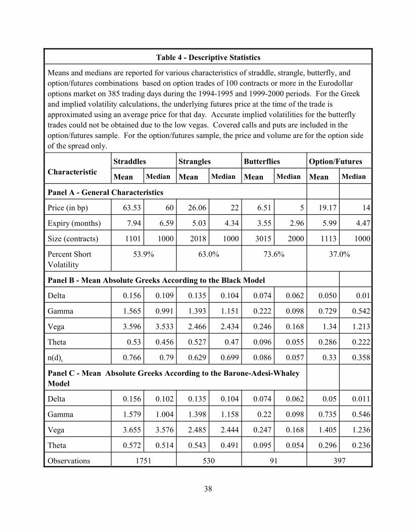
1.3. Descriptive Statistics

Descriptive statistics for straddles, strangles, and option/future combinations are presented in

Table 4. We also present statistics for butterflies since they are popular in the finance press though

not in practice. For these calculations we remove from the sample: (1) mid-curve options, (2)

straddles and strangles with a simultaneous futures trade (considered separately later), (3) positions

expiring within two weeks, and (4) a few observations with incomplete data.

Interestingly we observe large differences across the various trade designs in terms of

whether they are constructed to profit from increases or decreases in volatility. The percentage

which are short volatility (i.e., negative gamma and vega) ranges from 73.6% for butterflies to

37.6% for option/future combinations.14 The high short figure for butterflies is interesting. Possible

losses (at expiration) are unbounded on short straddles and strangles but bounded on short

butterflies so butterflies might be particularly attractive to traders shorting volatility for this reason.

On the other hand, if butterfly traders seek to exploit the normal smile shape, they would tend to buy

at-the-money options and sell away-from-the-money options leading to a butterfly which is long

volatility. The high percentage of short volatility positions on butterflies indicates that the latter is

not a popular trading strategy. Other short-long differences are discussed below. In interpreting

these percentages, it should be kept in mind that our data does not distinguish between trades

establishing and closing positions. If all positions were closed by a reversing trade, we would

observe short volatility trades 50% of time regardless of whether most were short or long initially.

The fact that 73.6% of butterflies are short volatility and 62.4% of option/futures combinations are

long probably means that these figures are higher for trades opening positions.15

Practitioner materials on option spreads and combinations often tout price minimization as

an objective. This implicitly assumes that the traders are net long (net buyers of options). More

importantly, it ignores the fact that the price equals the discounted value of the expected payout

using risk neutral probabilities. A quick look at the net prices in Table 4 is sufficient to reject the

hypothesis that traders seek to minimize the net price. Straddles which are the most popular are also

9

the most expensive. Butterflies are quite cheap since two options are bought and two sold but are

rarely traded. Moreover most butterfly positions are short.

Statistics for estimated Black and BW Greeks are presented in Panels B and C respectively.

Since neither the Eurodollar futures price at the time of the option trade nor the time of the trade are

recorded by Bear Brokerage’s observer, in calculating the Greeks, we approximate the underlying

futures price using an average of the open, settlement, high, and low prices that day.16 As shown in

Panel B of Table 4, most straddles, and strangles have low deltas but are not completely delta

neutral while most option/future combinations are close to delta neutral. Since gamma and vega

vary with time-to-expiration, it is more instructive to compare figures for n(d)c across trade types

than gamma and vega directly. Earlier we noted that among the seven volatility trades, the one with

the highest potential n(d)c value was a straddle at a strike equal to . At this strike n(d)c =

.7979 for the straddle. The median value of n(d)c for straddles is only slightly less than this limit at

.790 while the mean is .766. With a median n(d)c = .699 and mean =.629, n(d)c tends to be about

10 to 15% smaller for strangles than for straddles.

1.4. Volatility Patterns

One of the issues to be examined below is whether volatility trade designs are influenced by

the slope of the implied volatility smile. If traders view implied volatility differences as real, then

they may prefer to design their trades so that they short options with relatively high implied

volatilities and long those with low implied volatilities. If on the other hand, they view the implied

volatility differences as due to errors in calculation (specifically using Black Scholes model to

calculate volatility when it is inappropriate), then trade design should not be influenced by the smile.

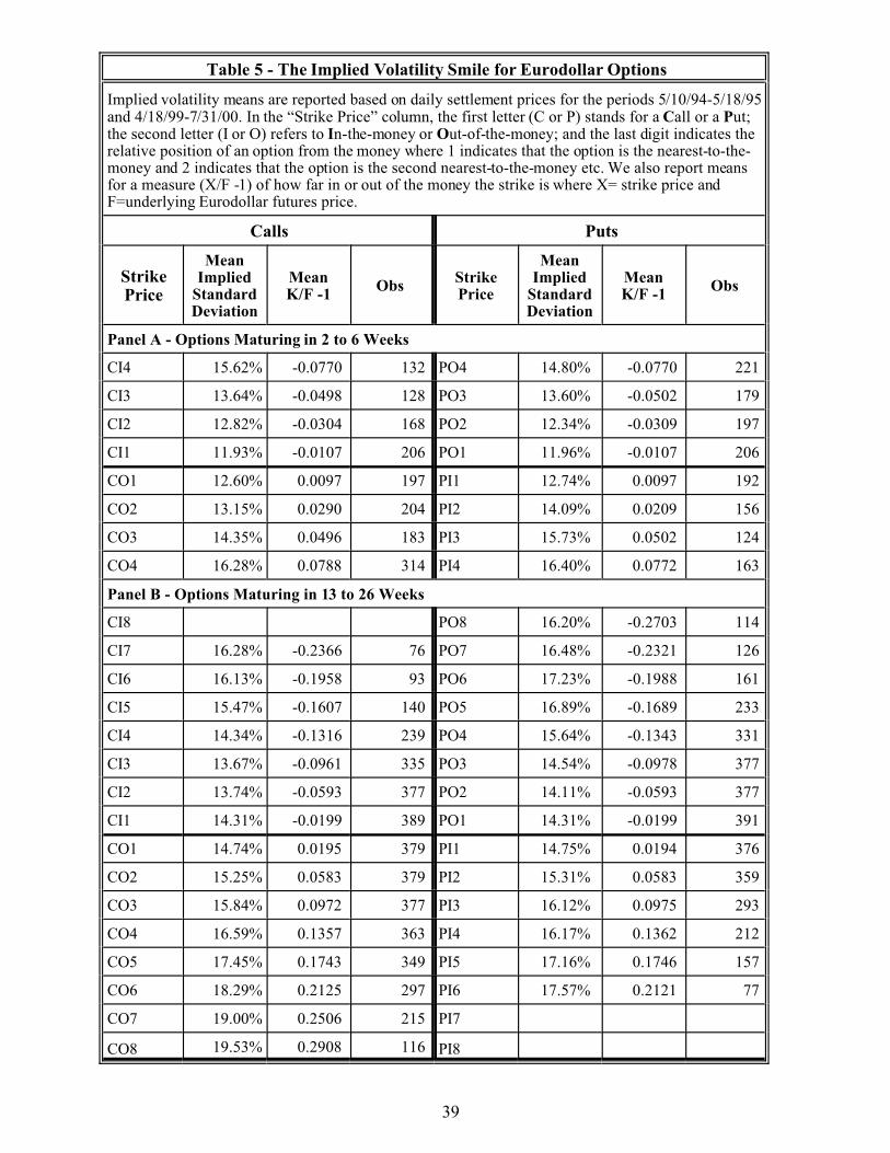
Accordingly, in Table 5 and Figure 1 we document the average smile pattern in implied volatilities

in the Eurodollar options market over our data period.17 For each option j on every day t, we obtain

the implied standard deviation, ISDj,t, as calculated by the CME and calculate the relative percentage

“moneyness” of option j’s strike price measured as (Xj,t/Ft)-1 where Xj,t is option j’s strike price and

10

Ft is the underlying futures price on day t. This is done for two different expiries: options maturing

in two to six weeks and options maturing in 13 to 26 weeks. Time series means of both ISD and

(X/F)-1 are reported in Table 5 and the former is graphed against the latter in Figure 1. The

following nomenclature is used in Table 4 to identify calls and puts and strike price groups j. The

first letter, “C” or “P,” indicates call or put, the second, “I” or “O”, indicates whether the option is

in or out of the money, and the last digit, “1" through “8", reports the strike price position relative to

the underlying futures price where “1" is the closest to the money and “8" is the furthest in- or out-

of-the-money. For example, CI3 indicates an in-the-money call option whose strike price is the

third strike below the futures price. We only report results for strikes traded on 75 or more days and

in Figure 1 we only show results for strikes between CI4 (or PO4) and CO4 (or PI4). As shown in

Figure 1, the implied volatilities display a standard smile pattern - generally rising as strikes further

from the underlying futures price are considered. The smile is steeper at the shorter maturity.

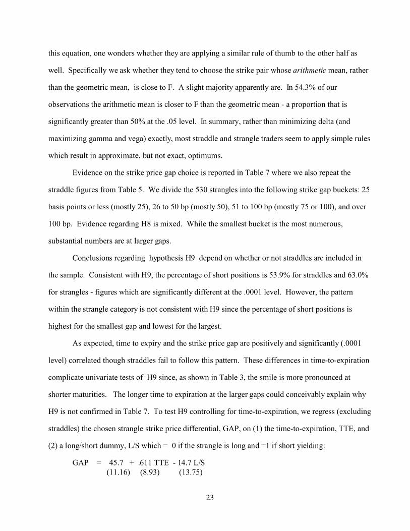
Figure 2 documents how the implied volatilities vary with the time-to-expiration. For this

we calculate the average implied volatility each day on the four at-the-money options for each

option expiry As shown in Figure 2, implied volatility generally rises with the time to expiration.

It has been noted by Whaley (2002), and Bakshi and Kapadia (2003) among others that in

the equity index options market implied volatilities tend to consistently exceed actual volatility so

that a strategy of shorting volatility tends to be profitable. During our sample periods, the

annualized volatility of daily returns was 10.1% for Eurodollar futures expiring in 2 to 6 weeks and

15.9% for futures expiring in 13 to 26 weeks. Over the longer 1990-2000 period, these two

volatilities were 9.1% and 15.2% respectively. Consequently, for 2 to 6 week options implied

volatilities tended to exceed actual volatilities slightly while there was little difference for 13 to 26

week options.

11

2. Straddle Design

We next investigate the design of the three most popular volatility trading strategies:

straddles, strangles and option/asset combinations starting with straddles. We consider three

straddle design issues: (1) which strike price to use, (2) whether to combine calls and puts in the

traditional 1-to-1 ratio or alter the ratio to achieve delta neutrality, and (3) whether to combine a

futures trade with the straddle to achieve delta neutrality. Except for Natenberg (1994), who shows

that delta .0 if the straddle is at-the-money, we find no discussions of straddle design issues in the

literature.

2.1. The Straddle Strike Choice

Consider first the strike price choice. As in Section 1, we presume that straddle traders

prefer designs that (1) maximize the straddle’s sensitivity to changes in actual and/or implied

volatility (gamma and vega) and (2) minimize sensitivity to the price of the underlying asset (delta).

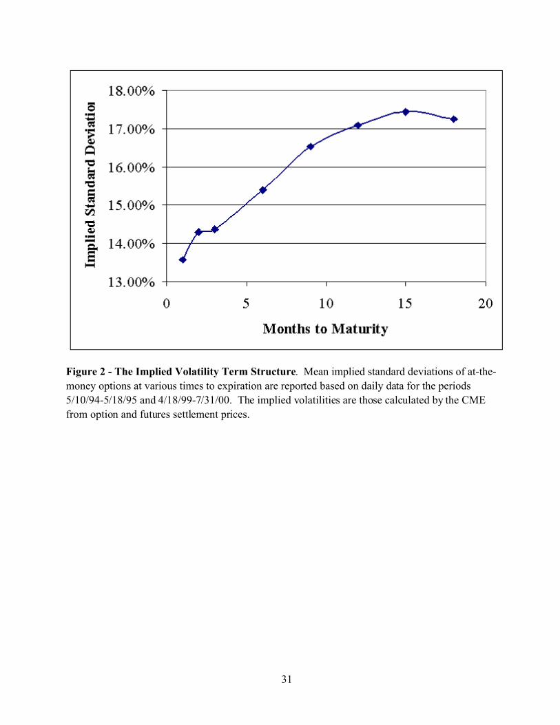
Fortunately, both objectives imply the same strike price choice. As shown in Section 1, a straddle’s

Black delta is zero (since N(d)=0) and vega and gamma are maximized (since n(d)c is maximized at

.7979) when the strike price is equal to where F is the underlying futures price, F is the

instantaneous volatility and t is the time-to-expiration. For short expiry options, the exponential

term is small so F* is just slightly above the current futures price, F. In our straddle data set, the

mean of F*-F is 7.3 basis points. For most straddles, the strike at which delta is equal to zero

according to the BW model is virtually identical. How delta, gamma, and vega vary with the chosen

strike is illustrated in Figure 3, where we graph a straddle’s Black delta, and gamma/vega (or n(d)c)

as functions of the strike price for the case when F = .16, t = .5 years, r=.065 and F=6.50.18 At

strikes below F*, a bought (sold) straddle’s delta is positive (negative) while it is negative (positive)

for strikes above F*. As the strike moves away from F* in either direction, gamma and vega are

reduced (in absolute terms) since n(d) falls.

12

Unfortunately, since only a limited number of strikes are traded, a strike exactly equal to F*

is rarely available. In the Eurodollar option market, options which expire in less than three months

are currently traded in strike increments of 12 or 13 basis points for the five or so strikes closest to

the underlying futures and in 25 basis point increments for the strikes further from the money.

Options with expiries exceeding three months are traded in increments of 25 basis points. Prior to

May 1995, all increments were 25 basis points regardless of the expiry. Suppose, as in our

examples above, F = .16, t = .5 years, and r=.065 and suppose F=6.60, so F*=6.642. The closest

available traded strikes are 6.50 and 6.75. If X=6.50, the Black delta of the straddle is +0.147

(+0.156 according to the BW model). If X=6.75, the Black delta= -0.109 (BW delta = -0.130). So

even if the trader chooses the strike closest to F*, some delta risk remains. Since F* is rarely a

traded strike, we focus attention on the traded strike which is closest to F* in log or percentage

terms which we label X*. It is easily shown that among the traded strikes, the absolute delta is

lowest and absolute vega and gamma are greatest at X*. We shall refer to F* as the “zero-delta”

strike, and refer to X* as the “delta-minimizing” strike. For comparisons, we also make use of the

closest-to-the-money strike, Xm. So while X* is the strike closest to F* in log terms, Xm is the strike

which is closest to F in log terms. For 71.4% of our straddle observations, X*=Xm.

The presumption that straddles traders seek to minimize delta and maximize gamma and

vega leads to our first hypothesis:

H1: Ceteris paribus, a straddle trader will tend to choose strike X* which is the

available strike at which the Black delta is minimized and the Black gamma and

vega are maximized.

Obviously, other objectives may lead to different choices.19 For instance, in deriving H1, we

have assumed that implied volatility, F, is the same at every strike price. As discussed above, if

implied volatility differs across strikes and if traders view these differences as real, rather than the

result of calculating implied volatility with the wrong model, then a long straddle trader may wish to

long strikes with relatively low implied volatilities and avoid those with relatively high implied

13

volatilities. Conversely, a short straddle trader may prefer to short strikes with relatively high

implied volatilities. Consequently, our second hypothesis is:

H2: Ceteris paribus, straddle traders will tend to chose strikes with high implied

volatilities for short positions and strikes with low implied volatilities for long

positions.

2.2. Straddle Strike Results

Results relevant to H1 are presented in Table 6. The basic result is that while the great

majority of straddles are constructed using close-to-the-money strikes so that delta is low and

gamma and vega high, it is not always the strike at which delta is minimized and gamma and vega

maximized . While 54.3 % of the 1751 straddles use X*, in 71.0% the strike is Xm, the strike

closest to the current futures price. As noted above, in 71.4% of our observations, X* = Xm. If we

restrict attention to the 435 observations when X*�Xm and the straddle’s strike is one or the other,

in 83.7% of these, the strike is Xm, rather than X*. In only 16.3% is it the delta minimizing strike,

X*. Hence, although the evidence indicates that straddle traders choose strikes with low Black

deltas, hypothesis H1 (that they minimize the Black delta) is rejected.20

What are the consequences of choosing Xm instead of X*? In the 364 cases in which

X*�Xm and the straddle’s strike = Xm, the average absolute Black delta is .115. If the straddle

traders had used X* instead, the average Black delta would have been only .052. In terms of the

BW model, the estimated delta is .118 while it would have been only .054 if the strike were X*.

While this delta difference is statistically significant at the .0001 level, whether it is economically

important is in the eye of the beholder. On the one hand, Delta is more than double the minimum

possible. On the other hand, at Xm the straddle’s delta is fairly low anyway. It makes less

difference in terms of gamma and vega whether X* or Xm is chosen. Specifically, the estimated vega

and gamma are about 0.9% higher at X*.

While most straddles are at Xm, not all are. In 436 or 24.9%% of our observed straddles, the

strike is neither X* nor Xm. In 83.9% of these, it is one of the next closest strikes, e.g., 5.75 or 6.25

14

if X*=Xm=6.00 and the time-to-expiration exceeds three months. In these, the average absolute

Black delta is .299 versus .097 if the strike had been X*. In only 70 of the 1751 cases (about 4%) of

the straddles, was the straddle’s strike more than one strike from X* and Xm. Particularly since

some of these may have been trades to close positions which were opened with close-to-the-money

strikes, it is clear that virtually all straddles are constructed close to the money.

In summary, most (71%) straddles are at the closest-to-the-money strike. In a majority of

cases, this is also the strike at which delta is minimized and gamma and vega are maximized

according to the Black and BW models. However, when faced with a choice between the closest-to-

the-money strike and the delta-minimizing strike, most straddle traders choose the strike which is

closest-to-the-money even though by doing so they accept some delta risk (and slightly lower

gammas and vegas) according to the Black model. Deep in-the-money or out-of-the-money

straddles are quite rare.

To test H2 we focus on those straddles (24.9% of our sample) when the strike is neither X*

or Xm. According to H2, if volatility traders are shorting (longing) volatility, they should prefer a

strike with high (low) implied volatility. Given the usual smile shape this could lead them to choose

strikes other than X* or Xm for short volatility, i.e., negative gamma-vega, positions. Let ISD be

the implied standard deviation at the chosen strike ,X, and ISD* and ISDm be the implied standard

deviations at X* and Xm. Consider the cases when X�X* and X�Xm. According to H2 for a short

straddle, ISD>ISD* and ISD>ISDm while for a long straddle we expect ISD<ISD* and ISD<ISDm.

Since we cannot observe ISD* and ISDm at the exact time of the trade, we compare implied

volatilities calculated from the previous day’s settlement prices viewing these as providing the

signal which is executed on day t. We have sufficient data to calculate estimates of ISD, ISD*, and

ISDm for 388 of our 436 observations.21

Contrary to H2, we observe no significant different between ISD and ISD* or between ISD

and ISDm. For the 206 short straddles, the mean ISD is .1605 while ISD* is .1593 and ISDm is

.1589. The differences are insignificant at any reasonable significance level. Results for the 182

15

long straddles are similar; the means are .1607, .1599, and .1598 for ISD, ISD*, and ISDm

respectively. The results are little changed if the ISDs are calculated using day t prices instead of

day t-1 or if we calculate ISD using the actual price of the straddle. Hence, H2 is not confirmed .

Again, however we caution that the power of this test is limited by the fact that we cannot observe

the ISDs at the exact time of the trade and some of these may be trades closing rather than opening

positions.

2.3. Making Straddles Delta Neutral

As noted above, because of the discrete nature of the traded strikes, straddles cannot

normally be made completely delta neutral based on the strike price alone. Indeed, even in those

cases when X=X*=Xm, the mean absolute Black (BW) delta is .095 (.096). This raises the question

whether straddle traders undertake other strategies to lower delta and if so what. We explore two

possibilities. One is altering the put/call ratio away from the traditional 1-to-1 ratio. If the call’s

delta is Dc and the put’s is Dp, a delta neutral position could be created by buying Dc/Dp puts for

each call purchased. This is the hypothetical straddle structure employed by Coval and Shumway

(2001). A likely problem with this strategy is liquidity. Traditional 1-to-1 straddles trade actively

and their prices are posted on the floor and broker screens. If a trader chooses a ratio other than 1-

to-1, she must either place two separate orders or a “generic” combination order.

We find that straddle traders clearly reject this strategy. Out of our 13,597 trades we only

observe three instances in which a straddle was constructed in a call/put ratio other than 1.0.

Alternatively straddles can be made delta neutral by adding futures. As with changing the

call/put ratio, adding futures to a straddle changes the position’s delta but does not affect its gamma,

vega, or theta. Consequently, a straddle trader can choose the strike with the desired gamma-vega

or other characteristics and then use futures to lower the delta. Since about 8.5% of straddle trades

are accompanied by a simultaneous futures trade, we next explore whether delta reduction is the

reason the futures are added.22 We hypothesize:

16

H3: If futures are traded simultaneously with a straddle, the straddle position’sabsolute delta including the futures will be lower than it would be without thefutures. In other words, futures will be bought (sold) when the straddle’s delta(ignoring the futures) is negative (positive).

Going a step further we also hypothesize,

H4: Futures will be bought (sold) in quantities which reduce the position’s deltaapproximately to zero.

This second hypothesis is a stronger version of the first considering the size of the futures position

as well as its sign.

If the purpose of the futures trade is to achieve delta neutrality, we would expect this

strategy to be employed when the straddle’s absolute delta without the futures is relatively high,

which occurs when the chosen strike is far from X*. Consequently, our third hypothesis is:

H5: Those straddles accompanied by a simultaneous futures trade will tend to be atstrikes further from F* and to have higher absolute deltas than the straddlestraded without futures.

2.4. Straddles with Futures: Results

To test H3, we compare deltas with and without the futures for those straddles which were

accompanied by a futures trade. Removing those observations involving midcurve options, options

maturing in less than two weeks, and trades where the size of the futures trade is unrecorded, our

sample (which was not part of the straddle sample in Tables 5 and 6) consists of 153 such straddles.

Confirming H3, in 142 or 92.8% of these, the straddle position’s absolute delta is reduced by

incorporating the futures trade. Moreover, eight of the eleven contrary trades were placed by the

same clearing firm. It appears that this firm, or one of its customers, was following a unique trading

strategy whose objective is unclear.

Turning to H4, i.e., whether adding the futures reduces the straddle position’s delta to zero,

we focus on the 142 observations in which delta is reduced. Calculated without the futures, the

mean absolute delta of the straddles alone is .264. When the combined delta is calculated including

17

the futures, the mean absolute Black delta is only .038. The median absolute Black delta without

the futures is .202 whereas with the futures it is only .023. It seems clear that the purpose of

combining a futures trade with a straddle is to reduce the position’s Black delta to close to zero.23

Finally, we hypothesized (H5) that straddle traders choose to combine futures with their

straddles when the chosen strike price is far in- or out-of-the-money, or more precisely when it is far

from F*, so that the absolute delta of the straddle alone is high. For the 904 straddles which were

not accompanied by a futures trade, the average absolute difference between the chosen strike price

X and the zero-delta strike price F* is13.8 basis points. For the straddles accompanied by a futures

trade, the mean difference between X and F* is 30.9 basis points or over twice as far from F* on

average. The difference is significant at the .0001 level so H5 is also confirmed. For the straddles

unaccompanied by a futures trade, the mean absolute delta is .156. For the straddles accompanied

by a futures trade, the mean absolute delta calculated without the futures is .264. Again the

difference is significant and H5 is confirmed.

In summary, we find that straddle traders tend to add a futures position to their straddles

when the chosen strike is far in- or out-of-the-money so that the straddle alone is far from delta

neutral, i.e., when they are exposed to substantial risk from a change in the price of the underlying

asset. In these cases, traders tend to long or short futures in quantities which reduce the Black delta

of their combined position approximately to zero. They virtually never alter the call/put ratio to

achieve delta neutrality.

3. Option/Futures Combinations

3.1. Delta Minimization and Covered Calls and Puts

In deriving our hypotheses regarding straddles above, we presumed that volatility traders

prefer delta neutral positions. Option/futures combinations provide a good test of this maintained

hypothesis. Writing covered calls (and sometimes puts), in which a trader shorts calls or puts and

simultaneously longs (for calls) or shorts (for puts) equal quantities of the underlying asset, is

18

perhaps the most discussed volatility strategy in derivatives textbooks and the practitioner literature.

Indeed the CBOE has recently instituted a “Buy Write” index which tracts the returns to this

strategy for equity index options. As far as we are aware, it is the only volatility strategy for which

such an index has been established. While possible losses on the option are bounded by this

strategy, the resulting positions are not delta-neutral unless the options are deep in the money.

Consequently, examining whether traders follow this prescription or instead construct delta-neutral

combinations provides evidence whether delta neutrality is truly important leading to the hypothesis:

H6: Traders will choose delta neutral ratios for option/futures combinations and avoidcovered calls and puts.

In 92 instances (all in 1999), Bear Brokerage’s observer failed to record the number of

futures contracts involved in these trades and data was incomplete for another observation. Of the

remaining 478 option/futures trades in our sample, in only 30 (6.3%) or is the option/futures ratio

1.0. Despite the attention that it receives in the literature, covered option writing appears fairly rare.

. Removing mid-curve options and those expiring in less than two weeks, reduces the sample

of combinations in which the futures/options ratio is not 1.0 to 364. In these, the mean estimated

absolute Black delta is only 024. By contrast in the 30 covered positions, the average delta was

.418. Particularly when one considers that some of our trades are probably closing positions created

earlier (in which case, delta may have drifted away from its initial value), it seems clear that

virtually all traders of option/futures combinations seek positions which are close to delta neutral.

H6 is confirmed.

Especially in light of our finding that straddles are virtually always in a 1-to-1 ratio, it is

interesting that the option position is usually evenly divisible by 100 while the futures position is

more irregular. For example, one trader bought 500 calls with an estimated delta of .3104 and

shorted 155 futures contracts for a net delta of .0004 per call. Apparently, traders think the liquidity

of odd lot positions is greater in the futures market.

19

3.2. Gamma and Vega and the Strike Choice

Option/futures combinations are instructive for gauging the importance of gamma and vega

in the design decisions since (in contrast to the straddle case) gamma and vega are determined

separately from the position’s delta. For option/futures combinations, as with straddles, Black

gammas and vegas are maximized if the chosen strike is X*, which is defined as the strike closest to

. Consequently, the question arises whether volatility traders continue to choose strikes

close to X* when delta minimization is not at issue. In 75.1% of straddles the observed strike was

either X* or Xm (which as we have seen is close to X*). In contrast, only 29.9% of option/futures

combinations are at one of these two strikes. In the case of straddles, the average difference

between the chosen strike and F* was 13.8 basis points. For option/futures combinations, it is 36.0

basis points. It seems clear that once other means of achieving delta neutrality are introduced,

traders venture further from at-the-money strikes. On the other hand, because gamma and vega are

fairly flat functions of the strike for options within a few strikes of X*, the impact on gamma and

vega is not great. The mean n(d) is .336, versus .399 at X* and n(d) exceeds .30 for 78.1% of the

option/futures combinations,

3 .3. The Smile and the Strike Choice

Since gamma/vega maximizing strikes are not always chosen, the question of what

influences the strike choice in option/asset combinations arises. Generalizing hypothesis H2, we

examine whether traders of option/futures combinations choose strikes with high implied volatilities

for short positions and low volatility strikes for long positions. As with straddles, we find little

evidence of such behavior. For short positions, the mean estimated implied volatility is 17.0% at

the chosen strike versus 16.8% at X*. While this difference is consistent with H2 (although it is not

significant at the .05 level), it is almost axiomatic given the normal U shape of the smile. More

telling are long positions. For these (the majority), the mean estimated implied volatility is 15.7% at

the chosen strike versus 15.3% X* - the opposite of what H2 would predict. Again H2 is rejected.

20

The fact that 62.6% of option/futures combinations have positive gammas and vegas is also

telling. As we have seen, constructing delta neutral straddles entails choosing close to the money

strikes which normally means strikes at the bottom of the smile. If implied volatilities are

important, this would be attractive for long positions but undesirable for short positions.

Consequently, if the smile is important to traders we would expect to see them seeking alterative

strategies to straddles for short but not long positions. The fact that the percentage of short

percentages is higher for straddles than option/futures combinations implies that the smile is not

relevant to this choice.

4. Strangles

4.1. Strangle Design Issues

In a long (short) strangle, the trader buys (sells) a call at one strike price and buys (sells) a

put at a lower strike. These two decisions may be viewed as (1) choosing the differential or gap

between the put and call prices (so that a straddle becomes a special case of a strangle with zero

gap) and (2) choosing the relation of the two strikes to the underlying asset or futures price.

Consider first the question of the distribution of the strikes around the underlying asset price holding

the call-put strike differential constant. As shown in Table 3, a strangle’s Black delta is zero iff

N(dc)+N(dp)=1. Since N(-x)=1-N(x), this occurs when dc = -dp where dc (dp) represents d defined in

terms of the call (put) strike. If volatility is the same for both the call and put, the dc = -dp condition

is met when ln(F/Xc) + ln (F/Xp) = -F2t yielding the result that the strangle delta is zero iff (XcXp).5 =

F* where F*= . In other words, a strangle is delta neutral iff the geometric mean of the two

strikes, which we designate as , equals F*. Likewise, gamma, and vega are maximized when

= F* . Of course, since the traded strikes are in increments of 12, 13 or (more commonly) 25 basis

points, a strike pair whose geometric mean is exactly equal to F* is not normally available but it is

easily shown that for a fixed differential, the Black delta is minimized by choosing the pair whose

geometric mean is closest to F*. Hence we hypothesize:

21

H7: For a given strike price differential, strangle traders will tend to choose the strikeprice pair at which the Black delta is minimized which is the pair whosegeometric mean is closest to F*.

Given our straddle results above, in which traders tended to choose Xm instead of X*, an obvious

alternative to H7 is that will be approximately equal to F, not F* leading to the alternative:

H7b: For a given strike price differential, strangle traders will tend to choose the strikeprice pair whose geometric mean is closest to F.

Next attention is turned to the differential or gap between strikes Xc and Xp. Note that

because a straddle can be viewed as a strangle with a zero differential, this analysis applies to the

straddle/strangle choice as well. Consider first the impact on the price and expected payout. Since

the payoff on a strangle is zero if the final asset price is between the two strikes, increasing the gap

between the two strikes in a strangle while holding the geometric mean constant,24 lowers the

expected payout and price. This is illustrated in Figure 4 where we graph the net price and expected

payoff of a strangle, according to the Black model, for different (assumed continuous) strike price

differentials for the case when F*=6.50, r=.065, F =.16, t=.5 and holding = F*.25

Of greater interest is the impact on the Greeks. If the geometric mean is held constant at F*,

increasing the call-put strike differential leaves the Black delta unchanged but reduces gamma and

vega. As shown in Table 2, for a given volatility and expiry, a strangle’s Black gamma and vega

are proportional to [n(d1c)+n(d1p)]. Consequently, if the call and put prices bracket F*, then

increasing the call-put differential holding constant reduces both n(dc) and n(dp) and hence

gamma and vega. as illustrated in Figure 4. The presumption that strangle traders seek to maximize

their strangle’s sensitivity to actual volatility (gamma) and/or implied volatility (vega) leads to the

hypothesis:

H8: Strangle traders will tend to choose small price gaps between the two strikes inorder to maximize gamma and/or vega.

Of course at the extreme this means choosing a straddle. Although straddles are far more common

than strangles, the fact that strangles are chosen at all means that the strike price gap decision

22

depends on more than gamma/vega maximization. We consider two possibilities: delta

minimization in combination with discrete strikes and the smile.

Implied volatilities are normally lowest for near-the-money strikes and higher on strikes

considerably in- or out-of-the-money. If these implied volatilities differences are viewed as real,

then traders wishing to speculate that actual volatility will be less (more) than implied volatility may

want to short strikes toward the top (bottom) of the smile, which means a large (small) strike gap if

the strangle is to be kept delta neutral yielding:

H9: Given a U-shaped volatility smile, traders will tend to construct short strangles

using large strike price gaps and long strangles using small price gaps.

We also expect the strike price differential to depend on the time to expiration. Since at

short times to expiration, far from the money options are thinly traded we expect smaller gaps at

shorter expiries.26

4.2. Strangle Results

Results for hypotheses H7 and H7b match our straddle results, that is, most strangle traders

choose strikes whose geometric mean, , is close to the current futures price even if this is not the

Black delta minimizing pair. For a given strike differential, in 57.0% of our observations, the

observed strike pair is that at which the Black delta is minimized. However, in 67.2% it is the pair

whose geometric mean is closest to F. The average difference between the geometric mean and F*

is -9.8 basis points while the average difference between the geometric mean and F is only -2.3 basis

points. In 63.2% of the observations, the geometric mean strike is closer to F than it is to F*, a

percentage which is significantly greater than 50% at the .0001 level. In summary, H7 is rejected in

favor of H7b. Strangle traders seek strikes which are close to the underlying futures, F, a strategy

which yields a low delta but not always the smallest.

According to our analysis, to minimize the Black delta, strangle traders should compare the

strikes’ geometric mean with F*. If traders are applying a simpler rule of thumb to the latter half of

23

this equation, one wonders whether they are applying a similar rule of thumb to the other half as

well. Specifically we ask whether they tend to choose the strike pair whose arithmetic mean, rather

than the geometric mean, is close to F. A slight majority apparently are. In 54.3% of our

observations the arithmetic mean is closer to F than the geometric mean - a proportion that is

significantly greater than 50% at the .05 level. In summary, rather than minimizing delta (and

maximizing gamma and vega) exactly, most straddle and strangle traders seem to apply simple rules

which result in approximate, but not exact, optimums.

Evidence on the strike price gap choice is reported in Table 7 where we also repeat the

straddle figures from Table 5. We divide the 530 strangles into the following strike gap buckets: 25

basis points or less (mostly 25), 26 to 50 bp (mostly 50), 51 to 100 bp (mostly 75 or 100), and over

100 bp. Evidence regarding H8 is mixed. While the smallest bucket is the most numerous,

substantial numbers are at larger gaps.

Conclusions regarding hypothesis H9 depend on whether or not straddles are included in

the sample. Consistent with H9, the percentage of short positions is 53.9% for straddles and 63.0%

for strangles - figures which are significantly different at the .0001 level. However, the pattern

within the strangle category is not consistent with H9 since the percentage of short positions is

highest for the smallest gap and lowest for the largest.

As expected, time to expiry and the strike price gap are positively and significantly (.0001

level) correlated though straddles fail to follow this pattern. These differences in time-to-expiration

complicate univariate tests of H9 since, as shown in Table 3, the smile is more pronounced at

shorter maturities. The longer time to expiration at the larger gaps could conceivably explain why

H9 is not confirmed in Table 7. To test H9 controlling for time-to-expiration, we regress (excluding

straddles) the chosen strangle strike price differential, GAP, on (1) the time-to-expiration, TTE, and

(2) a long/short dummy, L/S which = 0 if the strangle is long and =1 if short yielding:

GAP = 45.7 + .611 TTE - 14.7 L/S (11.16) (8.93) (13.75)

24

where t-statistics are shown in parentheses. Again H9 is rejected since the B/S coefficient is

negative.27 In summary, we find little evidence that strangle traders’ strike choices are influenced

by implied volatility differences.

An oft mentioned advantage of strangles in the practitioner literature is that they are cheaper

than straddles and the wider the gap, the lower the price. While we do not find this argument

convincing since the expected payout is reduced proportionally, it is consistent with the long/short

pattern across strike price gap buckets in Table 7. If price minimization is a goal, it should only be

so for long positions. Consequently, we would expect to see those taking long positions choosing

bigger gaps than those taking short positions. The results in Table 7 are consistent with this in that

the percentage of short positions falls from 66.7% for the smallest gap to 45.6% for the largest gap.

However, the strangle percentage does not fit this pattern.

5. The Straddle/Strangle Choice.

5.1. Determinants of the straddle/strangle choice

Lastly, we look at the volatility trader’s choice between a straddle and strangle. Since a

straddle may be viewed as a strangle with a zero strike price differential, part of this ground has

already been covered in Section 4. However, the fact that strikes are only traded in increments of

12, 13 or 25 basis points introduces another element. If F* is approximately midway between two

strikes, a strangle based on those two strikes will have a lower delta than a straddle based on either

strike alone. For instance, suppose F = .16, t =.500 years (6 months) , r=.065, and F=6.60 so F*=

6.64. If X=6.50, the delta of the straddle is 0.147. If X=6.75, the straddle’s delta is -0.109.

However, since the geometric mean of the two strikes is 6.62, the delta of the strangle using these

two strikes would be only 0.019. The presumption that delta neutrality is important to volatility

traders, leads to the hypothesis:

H10: Volatility traders will tend to choose a straddle when F* is close to a traded strikeand a strangle when F* is approximately midway between two traded strikes.

25

Given our previous results, we also test an alternative based on F instead of F*:

H10b: Volatility traders will tend to choose a straddle when F is close to a traded strikeand a strangle when F is approximately midway between two traded strikes.

To test H10 (H10b) we form a sample of all 124 (111) strangles with a strike price

differential of 25 basis points where F (F*)is between the two strikes.28 We then divide the 25 basis

point differential between Xp and Xc into five 5 basis point regions: (Xp, Xp+.05), (Xp+.05, Xp+.10),

(Xp+.10, Xp+.15),(Xp+.15, Xp+.20), (Xp+.20, Xc). According to H10 (H10b), we should observe

more strangles when F* (F) is falls in the middle quintile, (Xp+.10, Xp+.15), and few when it falls in

the first and fifth quintiles. If the null that the straddle-strangle choice is unrelated to where F or F*

falls relative to the traded strikes is correct, then the strangles should be roughly equally distributed

over the five quintiles. Results are reported in Figure 5. The distribution of F* relative to the

strikes roughly conforms to H10 in that we observe relatively few strangles with F* in the first and

fifth quintiles and the null that F* is randomly distributed across the quintiles is rejected at the .01

level . However, there are more observations in the fourth and fifth quintiles than expected. The

data are more consistent with H10b. There are very few observations in which F falls in the first

and fifth quintiles and the distribution is reasonably symmetric. The null that the distribution is

random is rejected at the .01 level. Performing a similar analysis for straddles, we find that in this

case as hypothesized, F tended to be bunched in quintiles closest to a traded strike. Again the

results are consistent with H10b and the null is rejected at the .01 level.

5.2. Probit estimations of the straddle/strangle choice

Finally, we explore determinants of the straddle/strangle choice using probit estimations.

Our choice variable is coded as 1 for strangles and 0 for straddles so a positive coefficient implies

that an increase in the variable means that a strangle design is more likely to be chosen. According

26

to hypothesis H10 (H10b) a straddle design is more likely to be chosen when F* (F) is close to a

traded strike. To test these, we include the variables Z* = |F*- closest strike| and Z=|F-closest

strike|. Hypotheses H10 and H10b imply positive coefficients for Z* and Z respectively. Since,

hypotheses H10 and H10b apply to cases when the underlying futures is either close to or between

the two strikes, we restrict our straddle/strangle sample to (1) all strangles where the gap between

the two strikes is 25 (or 12.5 adjusted to 25) basis points and either F or F* is between the two

strikes, and (2) all straddles at either of the two strikes closest to F or F*.

Given the normal shape of the implied volatility smile, hypothesis H9 implies that strangles

are more likely to be chosen if the trader is taking a short position and straddles if taking a long

position. To test this we include a variable, L/S, which is equal to 0 for a long position and 1 for a

short. H9 implies a positive coefficient. Given the time-to-expiration differences observed in Table

7, we include time-to-expiration, TTE (measured in years) as a control variable.

Results are presented in the column labeled Model 1 in Table 8. Hypothesis H10b is

confirmed at the .001 level while H10 is not. In other words, traders tend to choose straddles when

the underlying futures is close to a traded strike and a strangle when it is not. Supporting H9, the

coefficient of the L/S variable is positive and significant at the .05 level.

Because delta is more sensitive to the strike price choice at shorter maturities (i.e., gamma is

larger at shorter maturities) we expect Z (and/or Z*) to be more important at shorter expirations.

For example, suppose F=.16 and r=.065 and F*=6.625 which is halfway between the strikes of 6.50

and 6.75 so a strangle at these strikes is delta neutral. At a three month expiry, the absolute deltas of

straddles constructed using either strike are about .18. If the time-to-expiration is one year, the

absolute deltas are roughly half as large (.09) so whether the trader uses a straddle or a strangle is

not as important. Accordingly, we would expect the variables Z and/or Z* to be more important at

shorter expiries. This could explain why we tend to observe longer expiries on straddles - that

traders normally prefer straddles but switch to strangles at the shorter maturities if the underlying

asset price is roughly halfway between two strikes.

27

To test this hypothesis, we add the interaction variable TTE*Z to the probit. Our hypothesis

that Z matters more at shorter expiries implies a negative coefficient. Results are shown in the

column labeled Model 2 in Table 8. There is weak evidence to support our hypothesis in that the

interaction variable’s coefficient is negative and significant at the .10 level.

The positive and significant coefficient for the L/S variable is the first evidence in many tests

indicating that volatility traders base their trade designs on the smile. Accordingly, we scrutinize it

more closely. If traders view implied volatility differences as genuine, i.e., not due to calculation

errors, and seek to exploit them, we would expect any tendency to use straddles for long positions

and strangles for short positions to be stronger when the smile is steeply sloped. To test this, we

measure the slope of the smile as the ratio of implied volatilities at away-from-the-money strikes to

those at at-the-money strikes. Specifically, we calculate the average implied volatility, V1, that day

at strikes within 20 bp of the underlying futures, and the average implied volatility of all traded off-

the-money strikes, V2, and then calculate the smile slope, V2/V1. We then define

SMILE = V2/V1 if the straddle/strangle position is long and

= -(V2/V1) if the straddle/strangle position is short.

The hypothesis that the tendency to use straddles for long positions and strangles for short will be

stronger when the slope of the smile is steep implies a negative coefficient.

Results are reported in the final column of Table 8. As shown there the SMILE variable has

the wrong sign so there is no evidence that the tendency to use straddles for long positions and

strangles for short is stronger when the slope of the smile is steep. Overall therefore, we conclude

that there is little evidence that implied volatility differences influence volatility trade design.

6. Summary and Conclusions

Despite the fact that they are discussed in every derivatives text, are extensively covered in

the practitioner literature, and are actively traded (representing about 28% of large option trades),

volatility trades such as straddles, strangles, and option/asset combinations have received no

28

attention in the finance research literature. Using data from the Eurodollar options market we have

attempted to fill this gap.

Our first objective was to explain why some trades, such as strangles, are quite popular with

volatility traders while others, such as butterflies and covered calls and puts, are not. We found that

these preferences could be explained in terms of transaction costs and the spreads’ “Greeks.”

Our second objective was to examine the design of the three most popular strategies:

straddles, strangles, and option/futures combinations. We find that achieving approximate delta

neutrality is important to most volatility traders. For instance, traders generally eschew covered

calls and puts, which are not delta neutral, and construct option/futures combinations so that they

are almost exactly delta neutral. In constructing straddles, volatility traders tend to either choose

strikes resulting in low deltas or to combine the straddle with futures in a ratio which achieves delta

neutrality. Likewise, most strangle traders choose configurations which result in approximate delta

neutrality. Finally, in choosing between a straddle and a strangle, we find that volatility traders tend

to choose the strategy with the lower delta. However, our results indicate that most traders seek

only approximate delta neutrality. Faced with a choice between the strike or strikes closest to the

futures price, F, and those closest to the zero delta price, F*, traders normally choose the strike

(strikes) closest to F even if this strategy results in a slightly larger absolute Black or BW delta.

For most design decisions which we consider, the design choice which minimizes delta is

also that which maximizes gamma and vega so traders are not faced with a tradeoff between these

objectives. However, two design choices impact gamma and vega without changing delta: the strike

in option/futures combinations and the strike differential in strangles. In both cases, most traders

choose the gamma/vega maximizing design (or close to it) but a substantial minority do not.

Transaction costs and liquidity appear important explaining the rare use of butterflies, condors, and

guts, as well as the fact that straddle traders almost never change the call/put ratio away from 1.0.

We find little evidence that the slope of the smile influences volatility trade design, i.e., little

evidence that traders design straddles and strangles to exploit implied volatility differences. This

29

finding that traders apparently do not view implied volatility differences as exploitable is consistent

with the view that implied volatility differences are an artifact of calculation using an incorrect or

incomplete model - rather than reflecting real volatility differences.

30

Figure 1 - The Implied Volatility Smile. Mean implied standard deviations at various strike prices

are reported based on daily data for the periods 5/10/94-5/18/95 and 4/18/99-7/31/00. The implied

volatilities are those calculated by the CME from option and futures settlement prices for options

maturing in 2 to 4 weeks. Strike prices are expressed in relative terms as (X/F)-1 where X is the

strike price (in basis points) and F is the underlying futures price (in basis points).

31

Figure 2 - The Implied Volatility Term Structure. Mean implied standard deviations of at-the-

money options at various times to expiration are reported based on daily data for the periods

5/10/94-5/18/95 and 4/18/99-7/31/00. The implied volatilities are those calculated by the CME

from option and futures settlement prices.

32

Figure 3: Straddle Greeks as a Function of the Strike Price. Delta, gamma, vega, and

theta are simulated at different strike prices for a Eurodollar straddle using the Black model for the

case when F=6.00, r=6%, F =.18, and t=.5 (years). The Greeks are expressed as a percent of their

maximum values.

33

Figure 4: Strangle Greeks as a Function of the Strike Price Differential. Combination

characteristics are calculated for a Eurodollar strangle as a function of the gap between the two

strikes using the Black model for the case when r=6%, F=.18, t=.5 (years), F*=6.0, and the mean of

the two strikes is 6.0. The parameter values are expressed as a percent of their value when the

gap=0 (a straddle).

34

Figure 5. The gap in basis points between the two strike prices in close-to-the-money strangles

with a 25 bp (or 12.4 adjusted to 25 bp) differential is divided into five 5 basis point quintiles. The

number of observations in each quintile are shown for both quintiles based on the futures price, F,

and the zero delta price, F*.

35

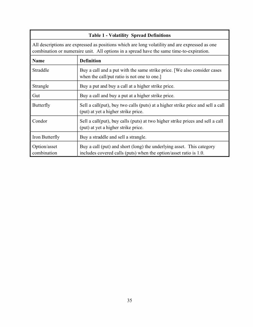
Table 1 - Volatility Spread Definitions

All descriptions are expressed as positions which are long volatility and are expressed as one

combination or numeraire unit. All options in a spread have the same time-to-expiration.

Name Definition

Straddle Buy a call and a put with the same strike price. [We also consider cases

when the call/put ratio is not one to one.]

Strangle Buy a put and buy a call at a higher strike price.

Gut Buy a call and buy a put at a higher strike price.

Butterfly Sell a call(put), buy two calls (puts) at a higher strike price and sell a call

(put) at yet a higher strike price.

Condor Sell a call(put), buy calls (puts) at two higher strike prices and sell a call

(put) at yet a higher strike price.

Iron Butterfly Buy a straddle and sell a strangle.

Option/asset

combination

Buy a call (put) and short (long) the underlying asset. This category

includes covered calls (puts) when the option/asset ratio is 1.0.

36

Table 2 - Volatility Spread Trading

Figures are based on all option trades of 100 contracts or more in the Eurodollar options market

on 385 trading days during the 1994-1995 and 1999-2000 periods. For each of the seven

volatility spreads, we report statistics on their trading as a percent of (1) all trades of 100

contracts or more, (2) all spread and combination trades, and (3) the six volatility spreads.

Combination

or Spread

Number of

Trades

Percent of all

large trades

Percent of all

spreads and

combinations

Percent of

volatility trades

Straddles 2379 17.50% 30.32% 62.16%

Strangles 676 4.97% 8.61% 17.66%

Options/futures 571 4.20% 7.97% 14.92%

Guts 10 0.07% 0.13% 0.26%

Butterflies 154 1.13% 1.96% 4.02%

Iron Butterflies 28 0.02% 0.36% 0.73%

Condors 9 0.07% 0.11% 0.24%

Table 3Black Model “Greeks” for Calls, Puts, Straddles, Strangles, and Butterflies

Derivatives according to Black’s options on futures model are presented where: F is the underlying futures price, X the exercise price,P the price of the option, F the volatility, t is the time-to-expiration, and r is the risk-free interest rate. d = [ln (F/X) + .5F2t] / F/t . N(.) represents the cumulative normal distribution, and n(.) the normal density. All derivatives are for positions which are longvolatility and are reversed for short positions. For straddles and strangles, the subscripts c and p designate the call and put strikesrespectively. For butterflies, the subscripts 1,2, and 3 designate the three different options. In this table calls and puts are defined interms of LIBOR, not 100-LIBOR. In the butterfly expression for delta, it is assumed the spread is constructed using calls.

Delta (MP/MF) Gamma (M2P/MF2) Vega (MP/MF) Theta (MP/Mt)

Call e-rtN(d)

Put e-rt[N(d)-1]

Straddle e-rt [2N(d)-1]

Strangle(& Gut)

e-rt [N(dc)+N(dp)-1]

Butterfly (& iron)

e-rt [-N(d1)+2N(d2)-N(d3)]

38

Table 4 - Descriptive Statistics

Means and medians are reported for various characteristics of straddle, strangle, butterfly, and

option/futures combinations based on option trades of 100 contracts or more in the Eurodollar

options market on 385 trading days during the 1994-1995 and 1999-2000 periods. For the Greek

and implied volatility calculations, the underlying futures price at the time of the trade is

approximated using an average price for that day. Accurate implied volatilities for the butterfly

trades could not be obtained due to the low vegas. Covered calls and puts are included in the

option/futures sample. For the option/futures sample, the price and volume are for the option side

of the spread only.

Characteristic

Straddles Strangles Butterflies Option/Futures

Mean Median Mean Median Mean Median Mean Median

Panel A - General Characteristics

Price (in bp) 63.53 60 26.06 22 6.51 5 19.17 14

Expiry (months) 7.94 6.59 5.03 4.34 3.55 2.96 5.99 4.47

Size (contracts) 1101 1000 2018 1000 3015 2000 1113 1000

Percent Short

Volatility

53.9% 63.0% 73.6% 37.0%

Panel B - Mean Absolute Greeks According to the Black Model

Delta 0.156 0.109 0.135 0.104 0.074 0.062 0.050 0.01

Gamma 1.565 0.991 1.393 1.151 0.222 0.098 0.729 0.542

Vega 3.596 3.533 2.466 2.434 0.246 0.168 1.34 1.213

Theta 0.53 0.456 0.527 0.47 0.096 0.055 0.286 0.222

n(d)c 0.766 0.79 0.629 0.699 0.086 0.057 0.33 0.358

Panel C - Mean Absolute Greeks According to the Barone-Adesi-Whaley

Model

Delta 0.156 0.102 0.135 0.104 0.074 0.062 0.05 0.011

Gamma 1.579 1.004 1.398 1.158 0.22 0.098 0.735 0.546

Vega 3.655 3.576 2.485 2.444 0.247 0.168 1.405 1.236

Theta 0.572 0.514 0.543 0.491 0.095 0.054 0.296 0.236

Observations 1751 530 91 397

39

Table 5 - The Implied Volatility Smile for Eurodollar Options

Implied volatility means are reported based on daily settlement prices for the periods 5/10/94-5/18/95and 4/18/99-7/31/00. In the “Strike Price” column, the first letter (C or P) stands for a Call or a Put;the second letter (I or O) refers to In-the-money or Out-of-the-money; and the last digit indicates therelative position of an option from the money where 1 indicates that the option is the nearest-to-the-money and 2 indicates that the option is the second nearest-to-the-money etc. We also report meansfor a measure (X/F -1) of how far in or out of the money the strike is where X= strike price andF=underlying Eurodollar futures price.

Calls Puts

StrikePrice

MeanImplied

StandardDeviation

MeanK/F -1

ObsStrikePrice

MeanImplied

StandardDeviation

MeanK/F -1

Obs

Panel A - Options Maturing in 2 to 6 Weeks

CI4 15.62% -0.0770 132 PO4 14.80% -0.0770 221

CI3 13.64% -0.0498 128 PO3 13.60% -0.0502 179

CI2 12.82% -0.0304 168 PO2 12.34% -0.0309 197

CI1 11.93% -0.0107 206 PO1 11.96% -0.0107 206

CO1 12.60% 0.0097 197 PI1 12.74% 0.0097 192

CO2 13.15% 0.0290 204 PI2 14.09% 0.0209 156

CO3 14.35% 0.0496 183 PI3 15.73% 0.0502 124

CO4 16.28% 0.0788 314 PI4 16.40% 0.0772 163

Panel B - Options Maturing in 13 to 26 Weeks

CI8 PO8 16.20% -0.2703 114

CI7 16.28% -0.2366 76 PO7 16.48% -0.2321 126

CI6 16.13% -0.1958 93 PO6 17.23% -0.1988 161

CI5 15.47% -0.1607 140 PO5 16.89% -0.1689 233

CI4 14.34% -0.1316 239 PO4 15.64% -0.1343 331

CI3 13.67% -0.0961 335 PO3 14.54% -0.0978 377

CI2 13.74% -0.0593 377 PO2 14.11% -0.0593 377

CI1 14.31% -0.0199 389 PO1 14.31% -0.0199 391

CO1 14.74% 0.0195 379 PI1 14.75% 0.0194 376

CO2 15.25% 0.0583 379 PI2 15.31% 0.0583 359

CO3 15.84% 0.0972 377 PI3 16.12% 0.0975 293

CO4 16.59% 0.1357 363 PI4 16.17% 0.1362 212

CO5 17.45% 0.1743 349 PI5 17.16% 0.1746 157

CO6 18.29% 0.2125 297 PI6 17.57% 0.2121 77

CO7 19.00% 0.2506 215 PI7

CO8 19.53% 0.2908 116 PI8

40

Table 6 - Straddle Strike Choices and Implications

We report on which strike prices are chosen for straddles and how this choice impacts the straddle’s delta according to the Black and

Barone-Adesi-Whaley models and gamma and vega according to the Black model. X is the chose strike price; X* is the strike (among

those traded) at which delta is minimized and gamma and vega maximized according to the Black model; and Xm is the available strike

which is closest to the underlying asset price (which may be the same as X*). For a given expiry, gamma and vega are proportional to

n(d), the value of the normal density function at strike price X.

Strike Number Percent

Mean

Absolute

Black

Delta

Mean

Abs.

Black

Delta if

X=X*

Mean

Absolute

BW

Delta

Mean

Abs. BW

Delta if

X=X*

Mean

n(d)

Mean

n(d)

if X=X*

X=X*=Xm 880 50.3% 0.1 0.1 0.1 0.1 0.75 0.75

X=X* but X�Xm 71 4.0% 0.05 0.05 0.05 0.05 0.764 0.76

X=Xm but X�X* 364 20.8% 0.115 0.05 0.118 0.05 0.713 0.77

Next closest strike to X* or Xm 366 20.9% 0.299 0.1 0.299 0.1 0.67 0.76

More than one strike from X* or Xm 70 4.0% 0.503 0.08 0.501 0.09 0.538 0.76

All 1751 100.0% 0.156 0.08 0.159 0.09 0.718 0.76

41

Table 7

Strangle (Straddle) Characteristics by Strike Price Differential

Mean values of several strangle (and straddle) characteristics are reported for different gaps or

differentials between the strike prices of the call and put. p-values are also reported for ANOVA

tests of the null hypothesis that the means do not differ by strike price differential.

Combination Characteristic

Strike Price Differential (D) (in basis

points)

Test of equality

null (p-value)

D=0

Stradd

les

D#25 25<D

#50

50<D#

100

100<

D

strangles

onlywith

straddles

Mean Differential (D) (in

basis points)

0 24 50 87.8 163.1 0 0

Time-to-Expiration (months) 7.94 3.37 5.01 6.89 6.79 0 0

Net Price (basis points) 63.53 24.71 27.93 29.6 19.19 0 0

Absolute Black Delta 0.156 0.151 0.13 0.135 0.1 0.02 0

n(d)c 0.766 0.715 0.679 0.601 0.456 0 0

Gamma 1.565 2.144 1.248 0.841 0.53 0 0

Vega 3.596 2.164 2.622 2.823 2.328 0 0

Theta 0.53 0.654 0.537 0.403 0.335 0 0

Percent Short Volatility

Positions

53.9% 66.7% 64.2% 63.2% 45.6% 0.09 0

Observations 1751 186 173 106 65

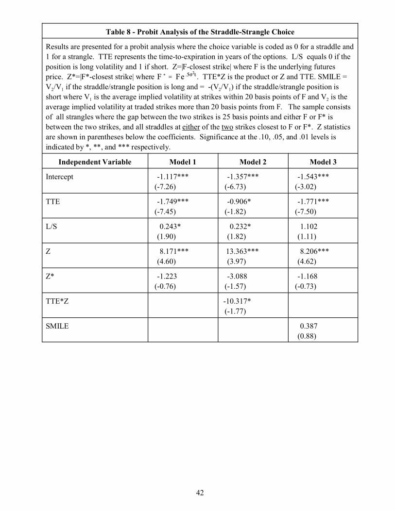
42

Table 8 - Probit Analysis of the Straddle-Strangle Choice

Results are presented for a probit analysis where the choice variable is coded as 0 for a straddle and

1 for a strangle. TTE represents the time-to-expiration in years of the options. L/S equals 0 if the

position is long volatility and 1 if short. Z=|F-closest strike| where F is the underlying futures

price. Z*=|F*-closest strike| where . TTE*Z is the product or Z and TTE. SMILE =

V2/V1 if the straddle/strangle position is long and = -(V2/V1) if the straddle/strangle position is

short where V1 is the average implied volatility at strikes within 20 basis points of F and V2 is the

average implied volatility at traded strikes more than 20 basis points from F. The sample consists

of all strangles where the gap between the two strikes is 25 basis points and either F or F* is

between the two strikes, and all straddles at either of the two strikes closest to F or F*. Z statistics

are shown in parentheses below the coefficients. Significance at the .10, .05, and .01 levels is

indicated by *, **, and *** respectively.

Independent Variable Model 1 Model 2 Model 3

Intercept -1.117***

(-7.26)

-1.357***

(-6.73)

-1.543***

(-3.02)

TTE -1.749***

(-7.45)

-0.906*

(-1.82)

-1.771***

(-7.50)

L/S 0.243*

(1.90)

0.232*

(1.82)

1.102

(1.11)

Z 8.171***

(4.60)

13.363***

(3.97)

8.206***

(4.62)

Z* -1.223

(-0.76)

-3.088

(-1.57)

-1.168

(-0.73)

TTE*Z -10.317*

(-1.77)

SMILE 0.387

(0.88)

43

REFERENCES

Bakshi, G., C. Cao, and Z. Chen, 1997, Empirical performance of alternative option pricing models,

Journal of Finance 52, (December), 2003-2049.

Bakshi, G. and K. Kapadia, 2003, Delta-hedged gains and the negative market volatility risk

premium, Review of Financial Studies 16 (Summer), 527-566.

Barone-Adesi, G. and R. Whaley, 1987, Efficient analytic approximation to american options

values, Journal of Finance 42, (June), 301-320.

Black, F., 1976, The pricing of commodity contracts, Journal of Financial Economics 3, (March),

176-179.

Chaput, J. S. and L. Ederington, 2003, Option spread and combination trading, Journal of

Derivatives 10, (Summer), 70-88.

Coval, J.A. and T. Shumway. 2001. Expected option returns, Journal of Finance 56, (June) 983-

1009.

Natenberg, S., 1994, Option Volatility and Pricing: Advanced Trading Strategies and Techniques,

Second Edition, Chicago, Probus.

Whaley, R.E., 2002, Return and risk of CBOE buy write monthly index, Journal of Derivatives 10,

(Winter), 35-42.

44

1. Eurodollar futures contracts are cash-settled contracts on the future 3-month LIBOR rate. Since LIBOR is a frequent benchmark rate for variable rate loans and interest rate swaps, hedgingopportunities abound so this is a very active market.

2. The 100 contract floor above which trades are recorded refers to each leg. For instance, ifan order is received for 80 straddles (80 calls and 80 puts), it is not recorded even though a totalof 160 options are traded while an order for 100 naked calls would be.

3. Traders also claim that orders for delta neutral positions receive get better execution thanseparate orders for the legs since the trader taking the other side also has a delta neutral positions. However, Chaput and Ederington (2003) find no evidence of lower effective spreads on deltaneutral straddles.

4. The CME distinguishes between covered calls and puts and delta-neutral asset-optioncombinations while we lump the two in Table 1. Any trades in which the ratio is not 1-to-1 areincluded in the latter group by the CME but we find that all are in fact approximately deltaneutral. Ratio spreads, which are common in our data set, can be designed so that their delta islow and gamma and vega are high and are sometimes regarded as volatility trades. We analyzethem in a separate paper since (1) they can but need not be designed as volatility trades, and (2)to include them here would substantially lengthen the paper since they involve number designissues.

5. Focusing on M and I assumes the cost structure is the same for all assets i. Since theunderlying asset in our market , Eurodollar futures, is much more actively traded than any oneoption, transaction costs on the futures are likely lower. Hence we expect transaction costs to besomewhat lower for covered call and put positions than for straddles, strangles, and guts andlower still for delta-neutral combinations.

6. When an option is exercised, a brokerage fee is normally levied as if the option had been sold. When the resulting futures position is closed, a further brokerage fee may be levied. In additionto any fees, there is also the time that the trader spends in arranging delivery and closing theposition.

7. In addition, in-the-money options tend to be less liquid than at-the-money and out-of-the-money options which would reinforce the same ranking. Avoiding early exercise may also enterthis calculation. If one leg of a combination is exercised by the counterparty then the volatilitytrader is exposed to risk on the remaining legs. Since this risk is greater on deep in-the-moneyoptions, traders shorting volatility might prefer strangles to equivalent guts and butterflies to ironbutterflies.

8. Based on conversations with traders and personal observations by one author who worked inthe Eurodollar options pit, Black’s model is by far the most popular. As we shall see below,there is also evidence from our data that this is the model being employed by most volatilitytraders in this market.

9. We ignore rho since it is negligible for all but very long term options. We discuss theta butnote that it is not a risk measure since time to expiration is known with certainly.

ENDNOTES

45

10. Longer term guts would be an exception to this statement.

11. As explained more fully in Chaput and Ederington (2002), option terminology in theEurodollar market can be confusing. Although Eurodollar futures and options are officiallyquoted in terms of 100-LIBOR, in calculating option values in the Eurodollar market, tradersgenerally use pricing models, such as the Black model, defined in terms of LIBOR, not 100-LIBOR. For instance, consider a Eurodollar call with an exercise price of 94.00. This call willbe exercised if the futures price (100-LIBOR) is greater than 94, or if LIBOR<6.00%. So a callin terms of 100-LIBOR is equivalent to a LIBOR put and vice versa. Hence, the price of aEurodollar call as officially quoted is obtained by setting F=LIBOR (not 100-LIBOR), X=6.00(not 94.00), and F defined in terms of LIBOR rate volatility into the pricing equation for a put. Indeed, this is the procedure used by the exchange to obtain its official volatility quotes. This isthe procedure used in Table 3 and throughout this paper.

12. Of course, other objectives could lead to different choices. For instance, traders seeking to exploit implied volatility differences or perceived mispricings might make other choices.Practitioner discussions of butterflies, in which some options are bought and some sold, tout theirlow net cost as an important advantage. Minimizing net cost implicitly assumes that the trader isnet long. More important, it overlooks the fact that the expected payout is also lower. Since theprice equals the discounted value of the expected payout using risk neutral probabilities, weexpect these two attributes, price and expected payout, to approximately balance out for mosttraders.

13. As we have seen, a delta-neutral option-futures combination should have lower transactioncosts that a delta-neutral straddle but its gamma and vega are no more than half that of thestraddle. Obtaining gamma-vega values comparable to a delta-neutral straddle would require atleast two numeraire unit option-futures trades which would entail higher transaction costs.

14. Of course for every short straddle or strangle order that we observe, someone (probably afloor trader) must take a long position in one or both options. Our data document an imbalanceamong those initiating the trades.

15. To explore this issue, we tried to match successive straddle trades with the same clearingmember, expiry, and strike and equivalent volumes with different signs. Out of our 1751straddles trades, we were only able to construct 112 pairs. Of these, 54.5% were long volatilitybased on the “opening” trade. - a figure which is not significantly different from zero.

16. In the Greek calculations, constant maturity 3-month T-bill rates are used for optionsexpiring in less than 4.5 months, 6-month T-Bills for options maturing in 4.5 to 7.5 months, 9-month for options expiring in 7.5 to 10.5 months and 1-year rates for all longer options.

17. The Futures Industry Institute data does not report implied volatilities for the April 1999 -September 1999 period so these figures are based on 1994-1995 and 2000.

18. For easier comparison, these are shown in relative rather than absolute terms in Figure 3 inthat each is expressed as a percentage of the derivative’s maximum value so that gamma, vega,and theta vary from 0 to1.0 and delta from -1 to +1.

46

19. For instance, a long straddle trader who thinks actual volatility will exceed implied volatilitybut also thinks a rise in the Eurodollar rate is more likely than a decline may want to choose a strike below X* in order to obtain a positive delta. On the other hand, for traders with shortpositions avoiding early exercise might provide another incentive to choose strikes close to F*. In a straddle, one option must be in-the-money. If a strike far from F* is chosen, one will bedeep in-the-money and early exercise would be more likely.

20. As noted above, since the futures price at the time of the trade is unknown, we use anaverage of the high, low, open, and settlement prices for F. Consequently, it is possible thatsome traders chose the strike closest to F* at the time of the trade but it is not the closest to F*based on our proxy. Similarly, we cannot distinguish trades which open and close positions andstrikes which were close to F* when the position was created may not be when the position isclosed. However, this applies equally to F and F* so should not affect the relative proportions ofX* and Xm.

21. A few options were lost because one of the ISDs could not be calculated because therelevant option did not trade that day.

22. The true percentage could be higher because we only observe the futures trades which werepart of the same order. If a trader placed one order for the straddle and a separate order for thefutures, it would be counted as a straddle without futures in our data set. These straddles werenot included in the samples in Tables 6 and 7.

23. The goal of reducing delta to near zero levels is also apparent in how the trades areconstructed. All but a couple of our straddle trades are in increments of 50 options, e.g., 250 or300 options, and most are in increments of 100. However 83.1% of the futures trades are insmaller increments. For instance, in one case 86 futures contracts are traded with 200 straddles. Calculated without the futures, the straddle’s Black delta is .427; with the futures it is -.003. Inanother case, 765 futures are traded with 1700 straddles. Without the futures, the straddle’s deltais .4428 but with only -.008.

24. Since the available strikes are in increments of 12.5 o5 25 basis points this cannot be doneprecisely in practice. For example if the strikes are 6.00 and 6.25, changing them to 5.75 and6.50 leaves the arithmetic average unchanged at 6.125 but changes the geometric average from6.124 to 6.114.

25. As in Figure 3, to aid comparison, the price is expressed as a percentage of its maximumvalue which occurs when the gap = 0, a straddle. Since, in percentage terms, the impact on priceand the expected payout is the same, this should not be an important consideration to moststrangle traders.

26. Also, for the same strikes, as time to expiration declines, dc and dp become larger inabsolute terms so [n(d)c + n(d)p] declines which tends to reduce gamma and vega. Since gammais proportional to 1/ , it still normally tends to increase but vega is proportional to sodeclines sharply.

27. Since hypothesis H9 implies that short volatility traders prefer strikes with relatively highimplied volatilities while long volatility traders prefer strikes with relatively low implied

47

volatilities, we also compared the average implied volatilities for the strangles with a spread of50 basis points with (1) the implied volatility on a straddle with the same midpoint and (2) astrangle with a 100 basis point strike differential. This was done separately for short and longpositions. No significant differences were observed.

28. Those cases when the strikes are quoted in 12.5 basis point increments are converted to 25basis point basis by doubling the spreads between F (or F*) and each strike.