HAL Id: halshs-00960664https://halshs.archives-ouvertes.fr/halshs-00960664

Preprint submitted on 18 Mar 2014

HAL is a multi-disciplinary open accessarchive for the deposit and dissemination of sci-entific research documents, whether they are pub-lished or not. The documents may come fromteaching and research institutions in France orabroad, or from public or private research centers.

L’archive ouverte pluridisciplinaire HAL, estdestinée au dépôt et à la diffusion de documentsscientifiques de niveau recherche, publiés ou non,émanant des établissements d’enseignement et derecherche français ou étrangers, des laboratoirespublics ou privés.

Exchange Rate Volatility, Financial Constraints andTrade: Empirical Evidence from Chinese Firms

Sandra Poncet, Jérôme Héricourt

To cite this version:Sandra Poncet, Jérôme Héricourt. Exchange Rate Volatility, Financial Constraints and Trade: Em-pirical Evidence from Chinese Firms. 2013. �halshs-00960664�

Exchange Rate Volatility, Financial Constraints and Trade: Empirical Evidence from Chinese Firms

Sandra PONCET Paris School of Economics

University Paris 1 CEPII

Jérôme HERICOURT University Lille

University Paris 1 CEPII

March 2013

G-MonD Working Paper n°31

For sustainable and inclusive world development

Exchange Rate Volatility, Financial Constraints andTrade: Empirical Evidence from Chinese Firms ∗

Jérôme Héricourt† and Sandra Poncet‡

March 13, 2013

Abstract

This paper studies how firm-level export performance is affected by Real ExchangeRate (RER) volatility and investigates whether this effect depends on existing financialconstraints. Our empirical analysis relies on export data for more than 100,000 Chineseexporters over the 2000-2006 period. We confirm a trade-deterring effect of RER volatility.We find that the value exported by firms, as well as their probability of entering newexport markets, decrease for destinations with a higher exchange rate volatility and thatthis effect is magnified for financially vulnerable firms. As expected, financial developmentseems to dampen this negative impact, especially on the intensive margin of export. Theseresults provide micro-founded evidence that financial constraints may play a key role indetermining the macro impact of RER volatility on real outcomes.

Keywords: Exchange rate volatility; financial development, exports.

JEL classification: F14, F31, L25.

∗We are especially grateful to Raphael Auer, Nicolas Berman, Sergey Nigay, Katrin Rabitsch, Glenn Ryapand participants at several seminars and conferences for very useful comments and discussions on earlier draftsof the paper. Part of this research was funded by the French Agence Nationale de la Recherche (ANR), undergrant ANR-11-JSH1 002 01. Any remaining errors are ours.†EQUIPPE-Universités de Lille, Centre d’Economie de la Sorbonne - Université de Paris 1 Panthéon-

Sorbonne and CEPII; Email: jerome.hericourt@univ-lille1.fr‡Corresponding author. Paris School of Economics - Université de Paris 1 Panthéon-Sorbonne and CEPII.

Email: sandra.poncet@univ-paris1.fr

1 Introduction

The increasing volatility of exchange rates after the collapse of the Bretton Woods agreements

has been a source of concern for both policymakers and academics. An increasing number of

countries, both emerging (e.g., China) and developed (e.g., euro area members) have chosen

more or less fixed exchange rate systems as a way to protect themselves from the effects of an

excessive volatility, especially on trade. In a context where firms are risk averse, exchange rate

risk increases trade costs and reduces the gains from international trade (Ethier, 1973). Initial

macroeconomic evidence on the effect of exchange rate volatility on trade has been however

quite mixed, concluding to an effect which is either significant but small or insignificant (see

Greenaway and Kneller, 2007, or Byrne et al., 2008, for a survey). Even Rose (2000), who

finds a very large effect of currency union on international trade, concludes to a small effect of

exchange rate volatility. However, more recent works have emphasized that these results could

be due both to an aggregation bias (Byrne et al., 2008; Broda and Romalis1, 2010) and an

excessive focus on richer countries with highly developed financial markets. Indeed, much more

substantial negative effects of the exchange rate volatility on trade are found for developing

countries (Grier and Smallwood, 2007).

There is still a strong lack of firm-level evidence on the impact of exchange rate volatility

on exporting behavior, and on how this relationship may be influenced by financial constraints,

which are likely to be much stronger and more binding in developing countries. A careful

firm-level study of these relationships may bring us some more clear-cut evidence regarding the

exacerbating role of exchange rate volatility for export costs, and how financial development

may help alleviate these additional costs. This paper aims at filling these gaps. We study the

impact of Real Exchange Rate (RER) volatility on exporting behavior and the way financial

constraints, together with financial development, shape this relationship at the firm level. Our

empirical estimations rely on export data for more than 100,000 Chinese exporters over the

2000-2006 period. China is a highly relevant case for several reasons. Firstly, the country

displays an especially high export rate given it size, leading to substantial exposure to exchange

rate fluctuations. Secondly, China is interesting because it is characterized by a low financial

development, but with a rather high regional heterogeneity, which will be useful to identify a

non-linear effect of exchange rate volatility depending on credit constraints. Finally, the Chinese1Broda and Romalis (2010) also address the issue on reverse causality between exchange rate volatility and

trade. Once the problem is controlled for, they still find a negative impact of volatility on trade, though reduced.

2

yuan was strongly pegged to the US dollar during practically the whole period considered 2,

implying that the volatility we identify is truly exogenous to Chinese economic developments.

We expect a negative impact of exchange rate volatility on trade through an increase in

the variable and sunk costs of exporting. The former effect is implicitly addressed in Ethier

(1973), and is the most intuitive one: exchange rate risk creates an uncertainty for the exporter’s

earnings in its own currency, which is similar to an increase in variable costs. But exchange rate

volatility may also increase the sunk costs of exports, which can be seen as a form of investment

in intangible capital. In practice, most investment expenditures are at least in part irreversible,

i.e. made of sunk costs that cannot be recovered if market conditions turn out to be worse

than expected. The combination of investment irreversibility and asymmetric adjustment costs

induces a negative relationship between price volatility and investment (Pindyck 1988, 1991),

especially in developing economies (see Pindyck and Solimano, 1993). In such a context, high

volatility has consistently proved to reduce growth and investment, especially private investment

(Ramey and Ramey, 1995; Aizenman and Marion, 1999; Schnabl, 2007). Bloom et al. (2007)

find similar results within a firm-level framework with partial irreversibility: higher uncertainty

reduces the responsiveness of investment to a firm-level demand shock.

It is however only recently that the macro literature explicitly identified a relationship

between credit constraints and the size of the impact of volatility. Aghion et al. (2009) show

that the local financial development plays a key role in the magnitude of the repercussions

linked to the exchange rate volatility. Relying on a panel of 83 countries over the 1960-2000

period, they show that the negative impact of RER volatility on productivity growth decreases

with a country’s financial development. Within an identical framework, but focusing on foreign

currency (dollar) liabilities, Benhima (2012) shows over a panel of 76 emerging and industrial

countries between 1995 and 2004 that the higher the share of foreign currency in external debt,

the more detrimental to growth exchange rate volatility is. This tends to support the idea that

the effect of RER volatility depends critically on the existence of credit constraints.

The link between volatility and export performance has been mostly investigated using

macro, and less frequently, disaggregated data at the sectoral level.3 Some papers do look at the

impact of the exchange rate on exporting firms (e. g., Berman et al., 2012, on France; Li et al.,2China defended a pegged exchange rate versus the US dollar until July 2005, when the government decided

to switch to a reference to a basket of other currencies. However, Frankel and Wei (2007) find the de factoregime remained a peg to a basket that put virtually all the weight on the dollar. Subsequently , some weightwas shifted to a few non-dollar currencies. In any case, the peg was still fairly strong in 2006.

3Some papers look at the impact of exchange rate variations on Chinese trade, including: Marquez andSchindler (2007), Ahmed (2009), Freund et al. (2011) and Cheung et al. (2012).

3

2012, and Park et al., 2010, on China), but they focus on the impact of the exchange rate level

rather than its volatility, and they do not account for the role of financial constraints. Firm-level

studies of the impact of exchange rate volatility on economic or trade performance for developing

countries are scarce. Carranza et al. (2003) find a negative impact of volatility on a sample

of 163 Peruvian firms; Cheung and Sengupta (2012) simultaneously study the impact of RER

variations and volatility on the share of exports-to-sales ratio for a sample of a few thousand

Indian non-financial sector firms, and find support for a negative effect of volatility. When

coming to the role of credit constraints in modelling the impact of RER volatility, especially on

export performance, research is almost nonexistent. To our knowledge, Caglayan and Demir

(2012) is the only firm-level study connecting firm productivity, exchange rate movements and

the issue of access to external finance. Based on a data set of 1,000 private Turkish firms, their

results support a negative impact of exchange rate volatility on productivity growth which is

downplayed by a better access to external finance. We depart from these previous works by

using a much wider data set of firms, by looking at whether firms move their exports away from

partners characterized by higher exchange rate volatility, and more importantly, by investigating

the presence of a non-linear effect of exchange rate volatility on performance depending on the

level of financial constraints, in the Chinese context. The latter is apprehended through two

complementary dimensions. First, we infer firm-level financial vulnerability from the financial

dependence of their activities. This approach was pioneered by Rajan and Zingales (1998) and

has proved to be a robust methodology to detect credit constraints and assess their evolution

(Kroszner et al., 2006, and Manova et al., 2011). Second, we exploit Chinese cross-provincial

heterogeneity to study how financial development may mitigate both credit constraints and

exchange rate volatility.

This paper contributes to the existing literature on various levels. First, we provide a

micro-founded investigation of Aghion et al. (2009)’s prediction that exchange rate volatility is

especially harmful to firms that have high liquidity needs when local financial development is

low. Second, our methodology allows to circumvent a number of endogeneity problems which

may have flawed some of the related studies. Indeed, the use of firm-level data mitigates

the issue of reverse causality from trade to exchange rate volatility (cf. Broda and Romalis,

2010), and the well-known simultaneity bias between exporting behavior and financial proxies

for credit constraints at the firm-level. It is very unlikely that a Chinese firm shock impacts

exchange rate volatility or measures of financial dependence based on data from US firms.

Besides, using cross-regional data within a single country instead of cross-country data makes4

the risk of confusion between financial development and other macro characteristics less severe.

Third, our results give insight into what the main sources of the apparent lack of macro impact

of exchange rate volatility could be: the level of financial constraints and financial development

appears indeed more important than the aggregation bias to explain this puzzle.

Our results are consistent with the aforementioned macro studies, especially Aghion et

al. (2009): both the value exported and the probability of entering a new export market

decrease for destinations with higher exchange rate volatility. This export-deterring effect is

magnified for financially vulnerable firms: for those most dependent on external finance, a

10% increase in RER volatility decreases the value exported by 14%, and the probability of

entering by 3%. As expected, financial development seems to dampen this negative impact,

especially on the intensive margin of export. These results are robust to various definitions of

trade margins, measures of RER volatility and financial dependence, subsamples, and to the

inclusion of additional controls. We therefore provide micro support to the macro literature

which points at financial development as a key determinant in identifying the impact of RER

volatility on real outcomes.

In the next section, we survey the different theoretical mechanisms underlying our approach,

before discussing our general methodology and presenting our database in section 3. In section

4, we start by presenting the results on the intensive margin, then on the extensive margin,

before introducing some robustness checks and a general discussion of our findings. Section 5

concludes.

2 Exchange Rate Volatility, Financial Constraints and Ex-

ports: Theoretical Underpinnings

Our approach stands at the crossroads of two strands of the literature. Firstly, there is a

rapidly increasing number of papers dealing with the behavior of firms which manufacture

and export several products to several destinations. It is now widely known that aggregate

exports are concentrated in a small number of major players (Eaton et al., 2004) and that large

exporters are involved in exporting more than one product (Bernard et al., 2011; Eckel et al.,

2011). Bernard et al. (2011) show that the proportion of multi-product firms that export, the

number of destinations for each product, and the range of products they export to each market

all increase in response to reduced variable trade costs. Even closer to our work is Berthou

and Fontagné (2013), who document the impact of the introduction of the euro on the export5

decisions of French firms, the number of products exported and average sales per product. Their

results point to a heterogeneous trade creation effect across euro area destinations: for those

firms exporting to destinations characterized by lower monetary policy coordination (that is,

higher exchange rate volatility) before 1999, exports grew by 12.8% following the introduction

of the euro, with 20% of the effect being due to an increase in the number of products exported.

By contrast, no effect arises regarding the decision to export. Conversely, they find a negative

effect on all three definitions of trade margins for euro area destinations with closer monetary

policy coordination before 1999, indicating that the additional competitive pressure did more

than offset the benefits of zero volatility.

Secondly, there is growing empirical evidence that credit constraints impact exporting be-

havior (Greenaway et al., 2007; Berman and Héricourt, 2010; Minetti and Zhu, 2011). These

papers consistently find that the effect is magnified when firms belong to industries relying

more on external finance (Minetti and Zhu, 2011), and in developing countries (Berman and

Héricourt, 2010) compared to developed ones (Greenaway et al., 2007). In a recent paper,

Manova (2013) incorporates financial frictions into a heterogeneous-firm model, before bringing

it to aggregate trade data. She finds that 20%-25% of the impact of credit constraints on trade

are driven by reductions in total (domestically sold and exported) output. Of the additional,

trade-specific effect, one third reflects limited firm entry into exporting, while two thirds are

due to contractions in the sales of exporters. Both extensive and intensive margins are therefore

affected by credit constraints.

Our paper explores the possibility of a negative impact of exchange rate volatility on trade,

proportionally stronger for financially vulnerable firms - and consequently weaker with high

levels of financial development. This can be generated by several mechanisms. One can think

of exchange rate risk creating uncertainty for the earnings of the exporter, which is equivalent

to uncertainty on variable trade costs. The results by Bernard et al. (2011) and Berthou and

Fontagné (2013) show that all trade margins are potentially concerned. The existence of well-

developed financial markets should allow agents to hedge exchange rate risk, thus dampening

or eliminating its negative effect on trade. This effect has not been clearly established, whether

empirically (Dominguez and Tesar, 2001) or theoretically (Demers, 1991), so it is interesting to

see if micro data help deliver clearer insights.

Another mechanism, which is more focused on the sunk costs of exports and therefore

especially fitted for the probability of exporting to new markets, may also be at work. On the

one hand, export capacity may indeed be considered as a type of investment in intangible capital6

(like R&D); on the other hand, exchange rate movements themselves give rise to additional

sunk costs (Greenaway and Kneller, 2007). The negative impact of exchange rate volatility on

exports can be rationalized through the asymmetry of adjustment costs leading to investment

irreversibility. When facing a real depreciation of its own currency, the current earnings of a

firm rise. The firm may use this additional income to fund the sunk costs of entering new

markets. But once these investments are made, it will be impossible to back out and recover

what they cost, even in the case of an abrupt subsequent currency appreciation. If firms are

credit constrained, they will face additional difficulties to fund new investments, and will be

even more reluctant to take the chance to engage in exports to markets characterized by highly

volatile exchange rates.

Several approaches may theoretically rationalize this mechanism. In Aizenman and Marion

(1999), the introduction of credit rationing leads to a nonlinearity in the intertemporal budget

constraint. In their framework, the supply of credit facing a developing country is bounded

by a credit ceiling, independently from the level of demand. The credit ceiling hampers the

expansion of investment in the high-demand state, without moderating the drop in investment

in the low-demand state. Thus, this asymmetric pattern implies that higher volatility reduces

the average rate of investment, and that this effect is magnified with credit constraints. An

alternative mechanism is proposed in Aghion et al. (2009). Suppose an exporter faces fixed

wage costs in the local currency. When the bilateral exchange rate vis-à-vis that of the exporting

market fluctuates, the exporter cannot completely pass the cost change through to the exporting

market, because of competitive pressures, for example. Then, exchange rate volatility leads to

fluctuations in profits, which can lower investments in an environment where external finance is

more costly than internal finance. Then, following an exchange rate appreciation, the current

earnings of firms decline. This reduces their ability to borrow in order to survive idiosyncratic

liquidity shocks and thereby invest in the longer term. Depreciations have the opposite effect.

However, the existence of a credit constraint implies that in general the positive effects of a

depreciation will not fully compensate for the negative effects of an appreciation. By reducing

the cost of external finance, financial development relaxes credit constraints and consequently

should decrease the impact of volatility on the sunk cost activity, in our case exports.

We can summarize the testable predictions from these models for export performance, that

is both the intensive (the export value) and the extensive (probability of entering the export

market) margin:

Testable Prediction 1. Export performance decreases with exchange rate volatility. Na-7

ming α the parameter of interest, we therefore expect the link between volatility on the one hand

and the exported value and the probability of entering the export market on the other hand, to

be negative: α < 0.

Testable Prediction 2. The negative impact of exchange rate volatility on export per-

formance is magnified for financially vulnerable firms. The sign of the interaction - hereafter

named β - between the volatility of the real exchange rate and financial vulnerability is expected

to be negative: β < 0.

Testable Prediction 3. By relaxing credit constraints, financial development decreases

the impact of exchange rate volatility on export performance, proportionally more for finan-

cially vulnerable firms. The expected signs on both interactions, between volatility and financial

development on the one hand (parameter γ), and between volatility, financial development and

financial vulnerability on the other hand (parameter δ), are positive: δ, γ > 0.

Note also that the relative size and significance of α in comparison with the other parameters

will give us interesting insight into the respective roles of the aforementioned aggregation bias

and heterogeneity in terms of financial development. More precisely, a smaller (or even non-

significant) α compared to β, γ and δ will suggest that the impact of exchange rate volatility

on exports is not unconditional, but emerges mainly because of the credit constraints of firms

and low financial development.

3 Data Sources and Empirical Methodology

3.1 Exchange Rate Volatility

Exchange rate volatility is computed as the yearly standard deviation of monthly log diffe-

rences in the real exchange rate. We compute the real exchange rate as the ratio of the nominal

exchange rate of the yuan with respect to the partner’s currency divided by the partner’s

price level. Monthly data on nominal exchange rates and prices are taken from the IFS. As

a robustness check, we consider two alternative measures of volatility, the two-year standard

deviation of monthly log differences in the real exchange rate and the yearly standard deviation

of monthly log differences from the HP detrended real exchange rate (Hodrick and Prescott,

1997).

8

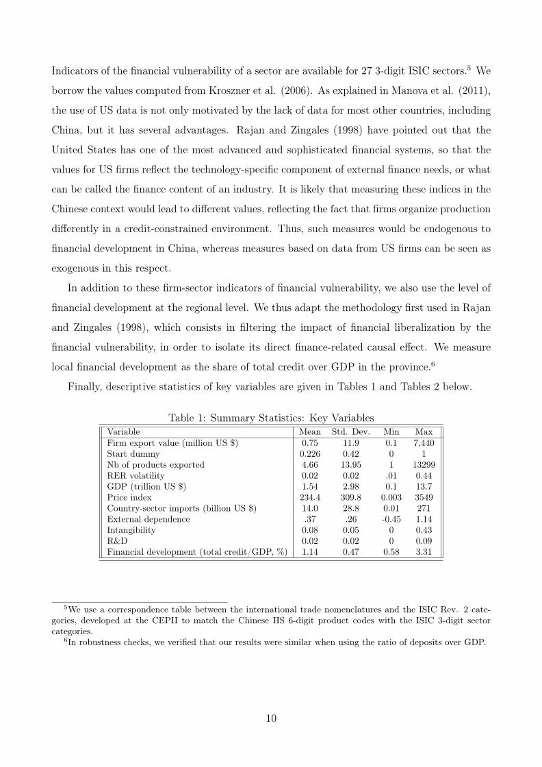
3.2 Trade Data

The main data source is a database collected by the Chinese Customs. It contains Chinese

firm-level yearly export flows by year, HS6 product and destination country, over the 2000-2006

period. It covers 113,368 exporting firms and 158 destinations.

3.3 Financial Vulnerability and Financial Development

We compute the firm-level financial vulnerability as the weighted average of the financial vul-

nerability of its activities, with the weights being the share of the sector in the exports by the

firm in 2000.4

FinV ulnF =ExportsFs∑sExportsFs

× FinV ulns (1)

We use three different measures of the financial vulnerability of a sector FinV ulns, in line

with other studies on the same topic. These variables are meant to capture the technological

characteristics of each sector which are exogenous to the financial environment of firms, and

determine the degree of reliance of the firms in each sector on external finance. While firms

in all industries may face liquidity constraints, there are systematic differences across sectors

in the relative importance of up-front costs and the lag between the time when production

expenses are incurred and revenues are realized. We capture these differences with a measure

of the external finance dependence in a sector (referred to hereafter as “financial dependence”),

constructed as the share of capital expenditures not financed out of cash flows from operations.

For robustness, we also use an indicator of the asset intangibility of firms. This measure is the

ratio of intangible assets to fixed assets. It thus captures another dimension of the dependence

of a firm on access to external financing: the difficulty to use assets as collateral in obtaining

financing. As a third indicator, we follow Manova et al. (2011) who use the share of R&D

spending in total sales (R&D), based on the fact that as a long-term investment, research and

development often implies greater reliance on external finance.

As is standard practice in the literature, these indicators are computed using data on all

publicly traded US-based companies from Compustat’s annual industrial files; the value of

the indicator in each sector is obtained as the median value among all firms in each sector.4In unreported results available upon request, we verify that our results hold when measuring the financial

vulnerability of a firm as the financial vulnerability of its main (ISIC) sector of activity, identified as the onewith the greatest export share in 2000.

9

Indicators of the financial vulnerability of a sector are available for 27 3-digit ISIC sectors.5 We

borrow the values computed from Kroszner et al. (2006). As explained in Manova et al. (2011),

the use of US data is not only motivated by the lack of data for most other countries, including

China, but it has several advantages. Rajan and Zingales (1998) have pointed out that the

United States has one of the most advanced and sophisticated financial systems, so that the

values for US firms reflect the technology-specific component of external finance needs, or what

can be called the finance content of an industry. It is likely that measuring these indices in the

Chinese context would lead to different values, reflecting the fact that firms organize production

differently in a credit-constrained environment. Thus, such measures would be endogenous to

financial development in China, whereas measures based on data from US firms can be seen as

exogenous in this respect.

In addition to these firm-sector indicators of financial vulnerability, we also use the level of

financial development at the regional level. We thus adapt the methodology first used in Rajan

and Zingales (1998), which consists in filtering the impact of financial liberalization by the

financial vulnerability, in order to isolate its direct finance-related causal effect. We measure

local financial development as the share of total credit over GDP in the province.6

Finally, descriptive statistics of key variables are given in Tables 1 and Tables 2 below.

Table 1: Summary Statistics: Key VariablesVariable Mean Std. Dev. Min MaxFirm export value (million US $) 0.75 11.9 0.1 7,440Start dummy 0.226 0.42 0 1Nb of products exported 4.66 13.95 1 13299RER volatility 0.02 0.02 .01 0.44GDP (trillion US $) 1.54 2.98 0.1 13.7Price index 234.4 309.8 0.003 3549Country-sector imports (billion US $) 14.0 28.8 0.01 271External dependence .37 .26 -0.45 1.14Intangibility 0.08 0.05 0 0.43R&D 0.02 0.02 0 0.09Financial development (total credit/GDP, %) 1.14 0.47 0.58 3.31

5We use a correspondence table between the international trade nomenclatures and the ISIC Rev. 2 cate-gories, developed at the CEPII to match the Chinese HS 6-digit product codes with the ISIC 3-digit sectorcategories.

6In robustness checks, we verified that our results were similar when using the ratio of deposits over GDP.

10

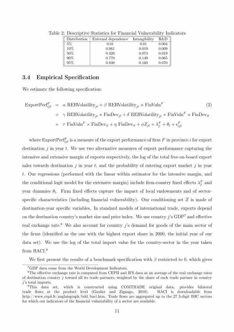
Table 2: Descriptive Statistics for Financial Vulnerability IndicatorsDistribution External dependence Intangibility R&D5% 0.01 0.01 0.00410% 0.061 0.019 0.00950% 0.326 0.074 0.01990% 0.770 0.149 0.06595% 0.838 0.160 0.070

3.4 Empirical Specification

We estimate the following specification:

ExportPerfFijt = α RERVolatilityjt + β RERVolatilityjt × FinVulnF (2)

+ γ RERVolatilityjt × FinDevjt + δ RERVolatilityjt × FinVulnF × FinDevit

+ τ FinVulnF × FinDevit + η FinDevit + φZjt + λFj + θt + εFijt

where ExportPerfFijt is a measure of the export performance of firm F in province i for export

destination j in year t. We use two alternative measures of export performance capturing the

intensive and extensive margin of exports respectively, the log of the total free-on-board export

sales towards destination j in year t, and the probability of entering export market j in year

t. Our regressions (performed with the linear within estimator for the intensive margin, and

the conditional logit model for the extensive margin) include firm-country fixed effects λFj and

year dummies θt. Firm fixed effects capture the impact of local endowments and of sector-

specific characteristics (including financial vulnerability). Our conditioning set Z is made of

destination-year specific variables. In standard models of international trade, exports depend

on the destination country’s market size and price index. We use country j’s GDP7 and effective

real exchange rate.8 We also account for country j’s demand for goods of the main sector of

the firms (identified as the one with the highest export share in 2000, the initial year of our

data set). We use the log of the total import value for the country-sector in the year taken

from BACI.9

We first present the results of a benchmark specification with β restricted to 0, which gives7GDP data come from the World Development Indicators.8The effective exchange rate is computed from CEPII and IFS data as an average of the real exchange rates

of destination country j toward all its trade partners, weighted by the share of each trade partner in countryj’s total imports.

9This data set, which is constructed using COMTRADE original data, provides bilateraltrade flows at the product level (Gaulier and Zignago, 2010). BACI is downloadable fromhttp://www.cepii.fr/anglaisgraph/bdd/baci.htm. Trade flows are aggregated up to the 27 3-digit ISIC sectorsfor which our indicators of the financial vulnerability of a sector are available.

11

us the unconditional effect of volatility on export performance. In a second step, we condition

the impact of volatility on the financial vulnerability of a firm by introducing an interaction

term between these two variables. Note that the financial vulnerability variable alone does not

appear, since it is captured by the firm-country fixed effects. We further modify our empirical

specification in a third and final step to allow α and β to vary depending on the development of

the local financial sector. In this case, our main parameters of interest are those on the double

interaction between RER volatility and financial development (γ) and on the triple interaction

between RER volatility, financial vulnerability and financial development (δ).

Finally, Moulton (1990) shows that regressions with more aggregate indicators on the right-

hand side could induce a downward bias in the estimation of standard errors. All regressions

are thus clustered at the province level10 using the Froot (1989) correction.

4 Results

We study the joint effects of exchange rate volatility and financial constraints on both margins

of trade, i.e. the size of exports by firm (the intensive margin) and the probability of entering

the export market (the extensive margin) separately.11

4.1 Intensive Margin

Table 3 presents the estimations of the impact of RER volatility on the value exported by

firms. Column (1) reports the estimates of a specification based only on the two proxies for

the destination countries’ market size and price index (which are significant and display the

expected positive signs), and column (2) investigates the unconditional relationship between

RER volatility and export performance. Column (3) includes an alternative measure of market

size, namely the country-sector imports, which appears positive and significant. The follow-

ing columns add a variable interacting RER volatility with a measure of firm-level financial

dependence. Columns (2) and (3) show that exchange rate volatility appears negatively asso-

ciated with export performance (i.e., the α parameter of Equation 2 is significant and negative).

Checking the robustness of this negative relationship with a volatility computed using the yearly

standard deviation of monthly log differences from the HP detrended real exchange rate, co-

lumn (1) of Table 10 in the Appendix confirms a negative impact of RER volatility. Overall, the10Since the province level is the most aggregated one (i.e., with the smallest number of clusters) in our case, it

gives the most possible conservative standard errors, and appears therefore as the safest choice we could make.11Robustness checks relying on alternative definitions for both margins are presented in the Appendix.

12

unconditional impact of RER volatility on the intensive margin is negative and significant.12

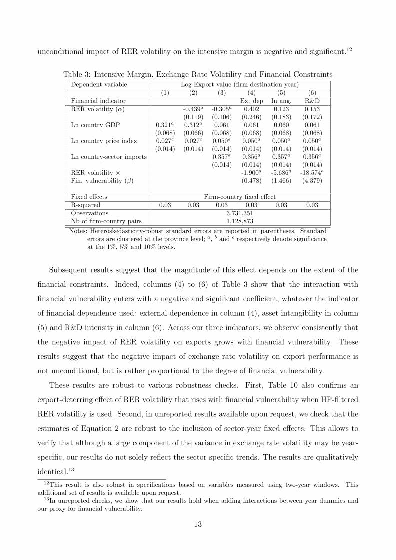
Table 3: Intensive Margin, Exchange Rate Volatility and Financial ConstraintsDependent variable Log Export value (firm-destination-year)

(1) (2) (3) (4) (5) (6)Financial indicator Ext dep Intang. R&DRER volatility (α) -0.439a -0.305a 0.402 0.123 0.153

(0.119) (0.106) (0.246) (0.183) (0.172)Ln country GDP 0.321a 0.312a 0.061 0.061 0.060 0.061

(0.068) (0.066) (0.068) (0.068) (0.068) (0.068)Ln country price index 0.027c 0.027c 0.050a 0.050a 0.050a 0.050a

(0.014) (0.014) (0.014) (0.014) (0.014) (0.014)Ln country-sector imports 0.357a 0.356a 0.357a 0.356a

(0.014) (0.014) (0.014) (0.014)RER volatility × -1.900a -5.686a -18.574aFin. vulnerability (β) (0.478) (1.466) (4.379)

Fixed effects Firm-country fixed effectR-squared 0.03 0.03 0.03 0.03 0.03 0.03Observations 3,731,351Nb of firm-country pairs 1,128,873Notes: Heteroskedasticity-robust standard errors are reported in parentheses. Standard

errors are clustered at the province level; a, b and c respectively denote significanceat the 1%, 5% and 10% levels.

Subsequent results suggest that the magnitude of this effect depends on the extent of the

financial constraints. Indeed, columns (4) to (6) of Table 3 show that the interaction with

financial vulnerability enters with a negative and significant coefficient, whatever the indicator

of financial dependence used: external dependence in column (4), asset intangibility in column

(5) and R&D intensity in column (6). Across our three indicators, we observe consistently that

the negative impact of RER volatility on exports grows with financial vulnerability. These

results suggest that the negative impact of exchange rate volatility on export performance is

not unconditional, but is rather proportional to the degree of financial vulnerability.

These results are robust to various robustness checks. First, Table 10 also confirms an

export-deterring effect of RER volatility that rises with financial vulnerability when HP-filtered

RER volatility is used. Second, in unreported results available upon request, we check that the

estimates of Equation 2 are robust to the inclusion of sector-year fixed effects. This allows to

verify that although a large component of the variance in exchange rate volatility may be year-

specific, our results do not solely reflect the sector-specific trends. The results are qualitatively

identical.13

12This result is also robust in specifications based on variables measured using two-year windows. Thisadditional set of results is available upon request.

13In unreported checks, we show that our results hold when adding interactions between year dummies andour proxy for financial vulnerability.

13

To illustrate these results, we can compare the decrease in the export performance due

to RER volatility for firms at the 10th and 90th percentiles of the distribution of financial

vulnerability. Table 2 above reports summary statistics on the distribution of the three indi-

cators of financial vulnerability. Using coefficients from column (4) in Table 3 for the intensive

margin, this means that, all things being equal, the negative effect of RER volatility on the

export value is -1.46 [=-1.90 × 0.770] at the 90th percentile of financial dependence compared

to -0.12 [=-1.90 × 0.061] at the 10th percentile. Hence, our results suggest that an additional

10 percent in yearly RER volatility may reduce the export value by 14 percent and 1.2 percent

in the two respective cases.

In Table 4, we check the robustness of our results to the inclusion of additional controls.

Financial vulnerability is measured using external dependence. We rely on our benchmark

specification from column (4) in Table 3. In column (1), we add the RER level to check that

our measured impact of RER volatility does not simply capture the impact level of RER. The

log of RER enters positively but fails to be significant. In column (2), we add the interactive

term between the level of RER and financial dependence. As expected, the interactive term

attracts a positive and significant coefficient. The reasoning is symmetrical to the one exposed

concerning RER volatility: financially constrained firms disproportionately take advantage of

a depreciating exchange rate.

14

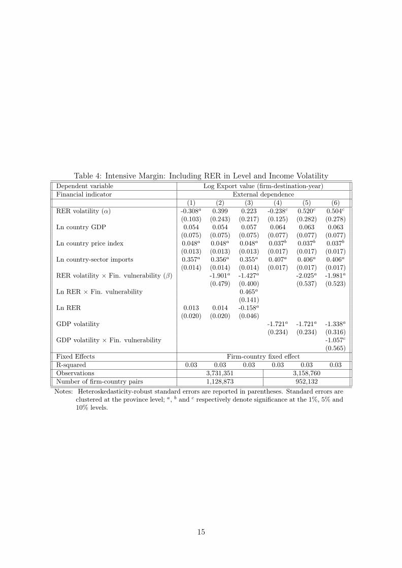
Table 4: Intensive Margin: Including RER in Level and Income VolatilityDependent variable Log Export value (firm-destination-year)Financial indicator External dependence

(1) (2) (3) (4) (5) (6)RER volatility (α) -0.308a 0.399 0.223 -0.238c 0.520c 0.504c

(0.103) (0.243) (0.217) (0.125) (0.282) (0.278)Ln country GDP 0.054 0.054 0.057 0.064 0.063 0.063

(0.075) (0.075) (0.075) (0.077) (0.077) (0.077)Ln country price index 0.048a 0.048a 0.048a 0.037b 0.037b 0.037b

(0.013) (0.013) (0.013) (0.017) (0.017) (0.017)Ln country-sector imports 0.357a 0.356a 0.355a 0.407a 0.406a 0.406a

(0.014) (0.014) (0.014) (0.017) (0.017) (0.017)RER volatility × Fin. vulnerability (β) -1.901a -1.427a -2.025a -1.981a

(0.479) (0.400) (0.537) (0.523)Ln RER × Fin. vulnerability 0.465a

(0.141)Ln RER 0.013 0.014 -0.158a

(0.020) (0.020) (0.046)GDP volatility -1.721a -1.721a -1.338a

(0.234) (0.234) (0.316)GDP volatility × Fin. vulnerability -1.057c

(0.565)Fixed Effects Firm-country fixed effectR-squared 0.03 0.03 0.03 0.03 0.03 0.03Observations 3,731,351 3,158,760Number of firm-country pairs 1,128,873 952,132Notes: Heteroskedasticity-robust standard errors are reported in parentheses. Standard errors are

clustered at the province level; a, b and c respectively denote significance at the 1%, 5% and10% levels.

15

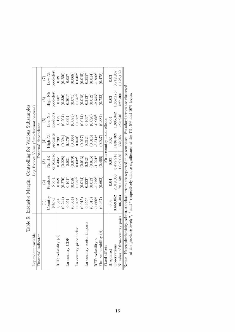
Table5:

IntensiveMargin:

Con

trollin

gforVarious

Subsam

ples

Dep

endent

variab

leLo

gExp

ortValue

(firm

-destina

tion

-year)

Finan

cial

indicator

Externa

ldep

endence

(1)

(2)

(3)

(4)

(5)

(6)

(7)

Cou

ntry

Produ

ctNoHK

HighNb

Low

Nb

HighNb

Low

Nb

Nb>

1Nb>

1or

Macao

prod

ucts

prod

ucts

prod

-dest

prod

-dest

RER

volatility(α

)0.384

0.359

0.435c

0.799c

0.179

0.507

0.391

(0.244)

(0.270)

(0.228)

(0.394)

(0.204)

(0.336)

(0.250)

Lncoun

tryGDP

0.051

0.101c

0.031

0.170b

0.004

0.201a

0.057

(0.064)

(0.058)

(0.079)

(0.066)

(0.085)

(0.071)

(0.068)

Lncoun

trypriceindex

0.048a

0.035b

0.032b

0.040b

0.056a

0.043b

0.048a

(0.015)

(0.014)

(0.013)

(0.017)

(0.014)

(0.018)

(0.015)

Lncoun

try-sector

impo

rts

0.355a

0.333a

0.342a

0.312a

0.409a

0.313a

0.355a

(0.013)

(0.013)

(0.015)

(0.013)

(0.020)

(0.012)

(0.014)

RER

volatility×

-1.866

a-1.722

a-1.921

a-3.314

a-0.968

b-2.545

a-1.892

a

Fin.vu

lnerab

ility

(β)

(0.467)

(0.602)

(0.466)

(0.927)

(0.382)

(0.722)

(0.478)

Fixed

effects

Firm-cou

ntry

fixed

effects

R-squ

ared

0.03

0.04

0.03

0.02

0.04

0.03

0.03

Observation

s3,659,052

2,019,033

3,472,215

1,836,309

1,895,042

1,862,175

3,719,937

Num

berof

firm-cou

ntry

pairs

1,106,403

781,138

1,059,036

532,927

595,946

527,300

1,128,139

Notes:Heteroskeda

sticity-robu

ststan

dard

errors

arerepo

rted

inpa

rentheses.

Stan

dard

errors

areclustered

attheprovince

level;

a,b

and

crespectively

deno

tesign

ificanceat

the1%

,5%

and10%

levels.

16

In the remaining columns, we verify that RER volatility does not act as a mere proxy for

economic fluctuations. We look at the repercussions of the volatility of the partner’s GDP. It

is computed as the standard deviation of year-to-year changes in quarterly GDP taken from

the IFS. As argued by Baum et al. (2004) and Grier and Smallwood (2007), foreign income

uncertainty may equally matter for trade. Consistently with their findings, GDP volatility

enters with a negative sign: income volatility has a significant deterrent effect on the value

exported. In columns (4) and (5), we see that this inclusion does not affect our benchmark

result of a negative impact of RER volatility that grows with financial vulnerability. In column

(6), we further include the interactive term between GDP volatility and financial dependence.

It is significant only at the 10% level (the negative impact of income volatility seems to vary,

but only weakly, with the level of credit constraints for a firm), while our main message on the

impact of RER volatility is not altered: the interaction between RER volatility and financial

dependence remains negative and significant.

Table 5 verifies that our results are robust to various changes in the sample. Here again,

financial vulnerability is measured using external dependence. Column (1) restricts the sample

to firms exporting to more than one country while column (2) concentrates on multi-product

firms. The point estimates are virtually unaffected. In column (3), we exclude observations

for Macao and Hong Kong since we are concerned that RER volatility may have different

implications in the case of these two “Greater China” territories than in that of other inter-

national partners. Once again, the negative coefficient on the interactive term between RER

volatility and financial vulnerability remains. In columns (4) to (7), we investigate whether our

results vary across firm-level productivity, proxied as the number of products or the number of

product-country pairs that a firm exports. This is done by regressing our main specification on

subsamples divided around the median of our productivity proxies. Our main findings remain

unchanged in all specifications, indicating that they apply to both low and high productivity

firms.

We now ask whether recent developments in China’s financial system have helped to reduce

the export losses from real exchange rate uncertainty. As previously mentioned, Aghion et al.

(2009) suggest that the effect of RER volatility depends critically on the level of local financial

development. We modify our empirical specification to allow β in Equation 2 to vary depending

on the development of the local financial sector. Our main parameter of interest is that on the

triple interaction between RER volatility, financial vulnerability and financial development (δ

in Equation 2).17

We first split the provinces into two groups depending on whether their financial development

is below or above the national median or the national mean in 2000 (the initial year of our

sample). The corresponding results are reported in columns (1) and (2) of Table 6. The

positive coefficient attracted by the interactive terms between RER volatility and financial

vulnerability in the case of provinces which are highly developed financially indicate that the

negative effect of RER volatility on the export value of firms is less present when credit is

abundant. In the following columns, we use the time-varying proxy for financial development

and interact it directly with RER volatility and financial dependence; the interaction between

local financial development and financial dependence is also included. We also add the level

of financial development and its interaction with RER volatility (the γ parameter) in columns

(4) and (5). In column (5), we include province-year fixed effects to account for the time-

varying characteristics of the local economy (including financial development, which drops as

a consequence). In this way, any variable correlated with financial development which could

impact the export performance of firms will be captured by these fixed effects, but should not

affect our coefficients of interest (β, γ and δ), unless its effect runs through a financial channel.

Our results confirm our previously measured negative interaction between RER volatility

and financial vulnerability, but suggest that the losses are mitigated by high local financial

development. In all columns, we find that financial development dampens the negative impact of

real exchange rate volatility on exports, the relaxation effect increasing with the level of sectoral

financial dependence of firms: the triple interaction between RER, financial dependence and

financial development is positive and significant. In other words, the positive offsetting effect

of financial development on RER volatility is magnified by the financial constraints for firms.

This result is in line with Aghion et al. (2009)’s observation that financial development reduces

the magnitude of performance deterioration induced by RER volatility. Conversely, there is

no evidence of an effect unconditional on financial constraints: the interaction between RER

volatility and financial development (γ) is insignificant.

As an additional check, we verify in Table 11 in the Appendix that our main results hold

when measuring the intensive margin based on the average export value for the firm-country

pair, computed as the ratio of total export value over the number of products exported (ex-

pressed in natural logarithms). All our key results remain: the negative impact of RER volatility

on the intensive margin increases with the credit constraints for firms, whatever definition of

financial vulnerability is used (columns (2) to (4)). Finally, the relaxing effect of financial de-

velopment also persists (columns (5) to (8)), with an even stronger significance compared to18

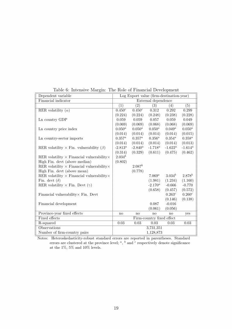
Table 6: Intensive Margin: The Role of Financial DevelopmentDependent variable Log Export value (firm-destination-year)Financial indicator External dependence

(1) (2) (3) (4) (5)RER volatility (α) 0.450c 0.450c 0.312 0.292 0.299

(0.224) (0.224) (0.248) (0.238) (0.228)Ln country GDP 0.059 0.059 0.057 0.059 0.049

(0.069) (0.069) (0.068) (0.068) (0.069)Ln country price index 0.050a 0.050a 0.050a 0.049a 0.050a

(0.014) (0.014) (0.014) (0.014) (0.015)Ln country-sector imports 0.357a 0.357a 0.356a 0.354a 0.358a

(0.014) (0.014) (0.014) (0.014) (0.013)RER volatility × Fin. vulnerability (β) -2.813a -2.840a -1.718a -1.622a -1.614a

(0.314) (0.329) (0.611) (0.475) (0.462)RER volatility × Financial vulnerability× 2.034bHigh Fin. devt (above median) (0.802)RER volatility × Financial vulnerability× 2.087bHigh Fin. devt (above mean) (0.778)RER volatility × Financial vulnerability× 7.069a 3.034b 2.878bFin. devt (δ) (1.981) (1.234) (1.160)RER volatility × Fin. Devt (γ) -2.170a -0.666 -0.770

(0.658) (0.457) (0.572)Financial vulnerability× Fin. Devt 0.263c 0.260c

(0.146) (0.138)Financial development 0.087 -0.016

(0.061) (0.056)Province-year fixed effects no no no no yesFixed effects Firm-country fixed effectR-squared 0.03 0.03 0.03 0.03 0.03Observations 3,731,351Number of firm-country pairs 1,128,873Notes: Heteroskedasticity-robust standard errors are reported in parentheses. Standard

errors are clustered at the province level; a, b and c respectively denote significanceat the 1%, 5% and 10% levels.

19

our preferred specification.

4.2 Extensive Margin

In this section, we assess the joint effect of RER volatility and financial constraints on the

extensive margin of trade, i.e. how they affect entry decisions. Columns (1) to (6) of Table 7

replicate Table 3, the explained variable being now the probability for a firm of entering the

export market j, that is, exporting to j in year t, while not having exported to j in year t− 1.

Once again, the unconditional impact of RER volatility (α parameter) appears negative and

significant (columns (2) and (3)), but adding interactive terms with each of our measures of firm-

level financial dependence shows that the magnitude of this effect is conditioned most of the time

by the extent of financial constraints (columns (4) to (6)): the β parameter appears negative

and highly significant, α becoming insignificant except when the financial dependence indicator

is the share of R&D spending in total sales. Quantitatively, the impact of an unconditional 10%

increase in exchange rate volatility (α parameter in column (3)) decreases the probability of

entering by 1.29%.14 Similarly, if we distinguish between firms at the 10th and 90th percentiles of

the distribution of financial vulnerability, we can compare the decrease in the extensive margin

due to RER volatility conditioning on financial vulnerability. Using coefficient β from column

(4), this means that, all things being equal, the negative effect of an additional 10% in RER

volatility on the probability of entering is -3% [(−0.223×0.77)×0.226× (1−0.226)] at the 90th

percentile of financial dependence, compared to -0.24% [(−0.223× 0.061)× 0.226× (1− 0.226)]

at the 10th percentile.

As before, we check the robustness of these results using the yearly standard deviation of

monthly log differences from the HP detrended real exchange rate as an alternative measure of

RER volatility (columns (5) to (8) of Table 10 in the Appendix), leading to similar qualitative

results. In unreported additional checks, we show that our results also hold when adding interac-

tions between year dummies and our proxies for financial vulnerability.15 Overall, the negative

impact of RER volatility on the probability of entry is magnified by financial vulnerability.

14This figure is obtained from the derivative of the choice probabilities (Train, 2003). The change in theprobability that a firm F will choose alternative X (start exporting) given a change in an observed factor ZF,X

entering the representative utility of that alternative (and holding the representative utility of other alternatives(no exporting) constant) is βZ × PF,X(1 − PF,X), with PF,X being the average probability that firm i willchoose alternative X (start exporting). Based on an average probability to start exporting of 22.6%, ourestimates suggest that the derivative of starting exporting with respect to an additional 10% in RER volatilityis −1.29% = −0.0735× 0.226× (1− 0.226).

15We were not able to implement regressions using sector-year dummies to control more systematically forsector-specific trends, the latter being too numerous to allow the maximization of the log-likelihood function.

20

Table7:

Extensive

Margin,

Excha

ngeRateVolatility

andFinan

cial

Con

straints

Dep

endent

variab

lePr(X

F i,j,t>

0|X

F i,j,t−

1=

0)

(1)

(2)

(3)

(4)

(5)

(6)

(7)

(8)

(9)

(10)

Finan

cial

indicator

Ext

dep

Intang

.R&D

Externa

ldep

endence

RER

volatility(α

)-0.864

a-0.735

a0.094

0.019

-0.454

a-0.779

a-0.197

-0.702

a0.024

(0.099)

(0.080)

(0.226)

(0.190)

(0.153)

(0.079)

(0.209)

(0.130)

(0.230)

Lncoun

tryGDP

0.072

0.051

-0.219

a-0.218

a-0.220

a-0.219

a-0.267

a-0.237

a-0.252

a-0.252

a

(0.055)

(0.055)

(0.057)

(0.057)

(0.057)

(0.057)

(0.070)

(0.072)

(0.072)

(0.072)

Lncoun

trypriceindex

0.099a

0.102a

0.125a

0.124a

0.125a

0.124a

0.109a

0.108a

0.077a

0.077a

(0.020)

(0.020)

(0.021)

(0.021)

(0.021)

(0.021)

(0.019)

(0.019)

(0.029)

(0.029)

Lncoun

try-sector

impo

rts

0.379a

0.378a

0.379a

0.379a

0.379a

0.372a

0.395a

0.394a

(0.033)

(0.033)

(0.033)

(0.033)

(0.033)

(0.033)

(0.053)

(0.053)

RER

volatility×

Fin.vu

lnerab

ility

(β)

-2.233

a-9.852

a-11.731a

-1.462

a-1.923

a

(0.431)

(1.973)

(3.612)

(0.374)

(0.370)

LnRER×

Fin.vu

lnerab

ility

1.252a

(0.231)

LnRER

0.101a

-0.377

a

(0.036)

(0.100)

GDP

volatility

0.076

0.950c

(0.193)

(0.574)

GDP

volatility×

Fin.vu

lnerab

ility

-2.433

b

(1.178)

Fixed

effects

Firm-cou

ntry

fixed

effect

Pseud

o-R-squ

ared

0.20

0.20

0.20

0.20

0.20

0.20

0.20

0.20

0.20

0.20

Observation

s8,801,335

8,801,335

6,996,782

Nbof

firm-cou

ntry

pairs

1,867,840

1,867,840

1,492,028

Notes:Heteroskeda

sticity-robu

ststan

dard

errors

arerepo

rted

inpa

rentheses.

Stan

dard

errors

areclusteredat

province

level;

a,b

and

cdeno

terespectively

sign

ificanceat

the1,

5an

d10%

levels.

21

In columns ((7) to (10)) of Table 7, we check as before the robustness of our results to

the inclusion of additional macro controls, namely the log of RER and GDP volatility. The

RER level enters positively and significantly (column (7)), and its interaction with financial

vulnerability is also correctly signed (positive) and significant (8): financially constrained firms

disproportionately take advantage of a depreciating exchange rate to enter the export market.

In columns (9) and (10), GDP volatility fails to enter significantly, but its interaction with

financial dependence is negative and significant: financially constrained firms are more harmed

by the instability of foreign demand. In any case, these additional estimates do not affect our

benchmark result of a negative impact of RER volatility that grows with financial vulnerability.

Table 8 checks the robustness of these results across various subsamples, financial vulner-

ability still being measured using external dependence. The results are unchanged for multi-

destination (column (1)) and multi-product (column(2)) firms, as well as when observations

for Macao and Hong Kong are excluded (column (3)): the β parameter remains negative and

significant, and entry on the export market is still disproportionately more harmed by exchange

rate volatility in the case of financially constrained firms. This result also holds when we divide

the sample around the median of our proxies for firm-level productivity, the number of prod-

ucts exported (columns (4) and (5)) or the number of product-destinations by firm (columns

(6) and (7)). Interestingly, the unconditional impact of RER volatility on entry (coefficient α)

also remains negative and significant for firms with a low number of products or a low number

of product-destinations: the probability of entry of low-diversified firms is also harmed by RER

volatility, even for a zero financial vulnerability.

22

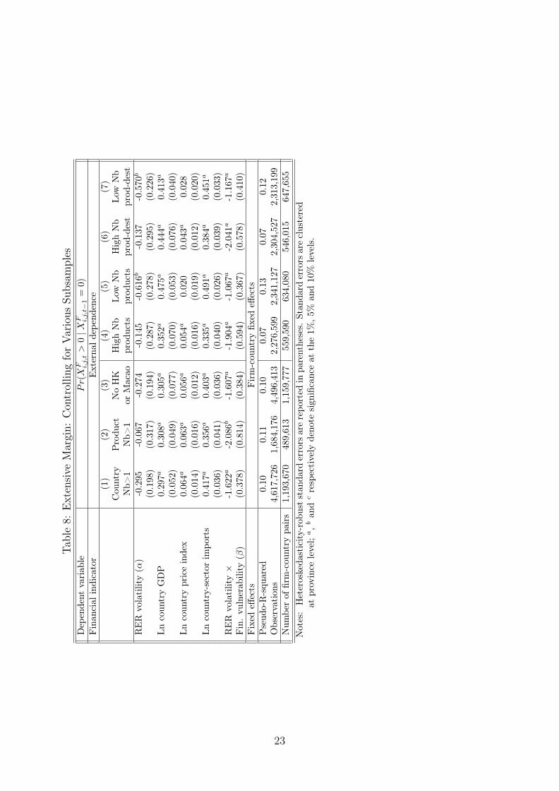
Table8:

Extensive

Margin:

Con

trollin

gforVarious

Subsam

ples

Dep

endent

variab

lePr(X

F i,j,t>

0|X

F i,j,t−

1=

0)

Finan

cial

indicator

Externa

ldep

endence

(1)

(2)

(3)

(4)

(5)

(6)

(7)

Cou

ntry

Produ

ctNoHK

HighNb

Low

Nb

HighNb

Low

Nb

Nb>

1Nb>

1or

Macao

prod

ucts

prod

ucts

prod

-dest

prod

-dest

RER

volatility(α

)-0.295

-0.067

-0.274

-0.145

-0.616

b-0.137

-0.570

b

(0.198)

(0.317)

(0.194)

(0.287)

(0.278)

(0.295)

(0.226)

Lncoun

tryGDP

0.297a

0.308a

0.305a

0.352a

0.475a

0.444a

0.413a

(0.052)

(0.049)

(0.077)

(0.070)

(0.053)

(0.076)

(0.040)

Lncoun

trypriceindex

0.064a

0.063a

0.056a

0.054a

0.020

0.043a

0.028

(0.014)

(0.016)

(0.012)

(0.016)

(0.019)

(0.012)

(0.020)

Lncoun

try-sector

impo

rts

0.417a

0.356a

0.403a

0.335a

0.491a

0.384a

0.451a

(0.036)

(0.041)

(0.036)

(0.040)

(0.026)

(0.039)

(0.033)

RER

volatility×

-1.622

a-2.086

b-1.607

a-1.904

a-1.067

a-2.041

a-1.167

a

Fin.vu

lnerab

ility

(β)

(0.378)

(0.814)

(0.384)

(0.594)

(0.367)

(0.578)

(0.410)

Fixed

effects

Firm-cou

ntry

fixed

effects

Pseud

o-R-squ

ared

0.10

0.11

0.10

0.07

0.13

0.07

0.12

Observation

s4,617,726

1,684,176

4,496,413

2,276,599

2,341,127

2,304,527

2,313,199

Num

berof

firm-cou

ntry

pairs

1,193,670

489,613

1,159,777

559,590

634,080

546,015

647,655

Notes:Heteroskeda

sticity-robu

ststan

dard

errors

arerepo

rted

inpa

rentheses.

Stan

dard

errors

areclustered

atprovince

level;

a,b

and

crespectively

deno

tesign

ificanceat

the1%

,5%

and10%

levels.

23

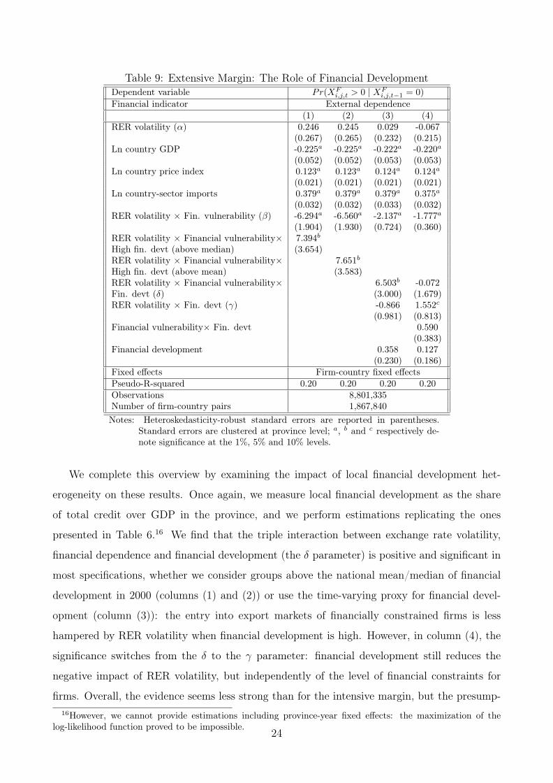
Table 9: Extensive Margin: The Role of Financial DevelopmentDependent variable Pr(XF

i,j,t > 0 | XFi,j,t−1 = 0)

Financial indicator External dependence(1) (2) (3) (4)

RER volatility (α) 0.246 0.245 0.029 -0.067(0.267) (0.265) (0.232) (0.215)

Ln country GDP -0.225a -0.225a -0.222a -0.220a(0.052) (0.052) (0.053) (0.053)

Ln country price index 0.123a 0.123a 0.124a 0.124a(0.021) (0.021) (0.021) (0.021)

Ln country-sector imports 0.379a 0.379a 0.379a 0.375a(0.032) (0.032) (0.033) (0.032)

RER volatility × Fin. vulnerability (β) -6.294a -6.560a -2.137a -1.777a(1.904) (1.930) (0.724) (0.360)

RER volatility × Financial vulnerability× 7.394bHigh fin. devt (above median) (3.654)RER volatility × Financial vulnerability× 7.651bHigh fin. devt (above mean) (3.583)RER volatility × Financial vulnerability× 6.503b -0.072Fin. devt (δ) (3.000) (1.679)RER volatility × Fin. devt (γ) -0.866 1.552c

(0.981) (0.813)Financial vulnerability× Fin. devt 0.590

(0.383)Financial development 0.358 0.127

(0.230) (0.186)Fixed effects Firm-country fixed effectsPseudo-R-squared 0.20 0.20 0.20 0.20Observations 8,801,335Number of firm-country pairs 1,867,840Notes: Heteroskedasticity-robust standard errors are reported in parentheses.

Standard errors are clustered at province level; a, b and c respectively de-note significance at the 1%, 5% and 10% levels.

We complete this overview by examining the impact of local financial development het-

erogeneity on these results. Once again, we measure local financial development as the share

of total credit over GDP in the province, and we perform estimations replicating the ones

presented in Table 6.16 We find that the triple interaction between exchange rate volatility,

financial dependence and financial development (the δ parameter) is positive and significant in

most specifications, whether we consider groups above the national mean/median of financial

development in 2000 (columns (1) and (2)) or use the time-varying proxy for financial devel-

opment (column (3)): the entry into export markets of financially constrained firms is less

hampered by RER volatility when financial development is high. However, in column (4), the

significance switches from the δ to the γ parameter: financial development still reduces the

negative impact of RER volatility, but independently of the level of financial constraints for

firms. Overall, the evidence seems less strong than for the intensive margin, but the presump-16However, we cannot provide estimations including province-year fixed effects: the maximization of the

log-likelihood function proved to be impossible.24

tion that financial development reduces the magnitude of performance deterioration induced

by RER volatility remains, along the lines of Aghion et al. (2009).

We check how our results behave using the probability of simply being an exporter at

the firm-destination-year level, instead of the probability of entering the export market, as

the definition of the extensive margin. Results which are still based on a conditional logit

specification with firm-country fixed effects are reported in Table 12 in the Appendix. These

results are qualitatively identical to the ones presented in Tables 7 and 9 above: we find some

evidence of an unconditional negative impact of RER volatility (column (1)). This negative

impact is once again magnified by firm-level financial dependence (columns (2) to (4)). Finally,

there is still some evidence that financial development produces a significant relaxation effect

in this context (columns (5) to (8)).

Finally, Table 13 in the Appendix reports the results of an alternative definition of the

extensive margin, namely the (log) number of HS6 products shipped to a country, in the spirit of

Manova et al. (2011). We still find a negative impact of RER volatility on export performance,

which is magnified for financially vulnerable firms. The evidence is much weaker regarding the

relaxing impact of financial development: the δ coefficient is correctly signed (positive), but

fails to be significant.

4.3 Additional Robustness Tests and General Discussion

Our empirical work so far has exploited the variation in export performance over time and across

destinations for firms of different sectors. Since a great proportion of the firms in our sample

export goods to more than one ISIC 3-digit sector, in what follows we also use the variation

across sectors, within firms. Our proxy for the intensive margin becomes the (log) export

value of the firm for a given sector/country pair in a year. The extensive margin is defined

as the (log) number of HS6 products for a given sector/country pair in a year. Otherwise

identical to Equation 2, these regressions include firm-sector-country fixed effects, so that the

coefficients are thus identified purely from the within variation in export performance, across

sector-country pairs, within multi-sector firms. Therefore, our estimates apprehend the way in

which firms choose to allocate their limited financial resources between different sector-country

export markets. This ensures that our results are not driven by some endogenous sorting of

single-sector firms into sectors and export markets for reasons other than credit constraints. The

results are reported in Tables 14 and 15, for the intensive and extensive margin respectively. In

both cases, exchange rate volatility impacts export performance negatively, disproportionately25

more for financially vulnerable firms. There is still a relaxing impact of financial development

for this specific definition of the intensive margin. However, no evidence of such an effect of

financial development can be identified for the range of products exported.

In additional, unreported checks available upon request, we assess the robustness of our

results to the exclusion of the USA as an export destination in the sample. This allows us to

make sure that our results are not biased by the presence of the country toward which volatility

is very reduced by construction during most of the period considered. Similarly, we perform

additional estimates excluding the years 2005 and 2006 to check whether the switch from a

pegging to the US dollar only to a basket of several currencies in July 2005 could impact our

results. In both exercises, our results remain qualitatively identical.

Moreover, we verify that our results hold for exporters irrespective of their ownership struc-

ture (whether domestic or foreign). We also perform estimations on a subsample excluding

intermediary firms. Indeed, our measure of financial constraints may be less relevant for those

firms which do not produce the goods they sell, since it is computed from information based

on production technology. We follow Ahn et al.’s (2011) approach to identify them based on

Chinese characters in the name of the firm which mean “importer”, “exporter”, and/or “trad-

ing” in English. 17 We also estimate specifications adding firm-country level imports from the

countries where the firm is also exporting. In all these checks, once again, the negative impact

of exchange rate volatility appears magnified for financially vulnerable firms, and relaxed by a

high level of financial development.

Finally, we also verify that the differentiated impact of RER volatility depending on financial

development does not simply reflect a correlation between financial development and trade costs.

It could be that provinces with a more developed financial system also benefit from easier and

cheaper international access: in this case, our results may rather identify an uncertainty related

to distance. We replicate our benchmark result looking at the double interaction between RER

volatility and financial dependence (column (4) of Tables 3 and 7) and the triple interaction

depending on financial development (columns (3) and (4) of Tables 6 and 9) when adding

interactive terms with three proxies for the geographical trade advantages that are coastal

location, western location and distance to partner country18, respectively. Our findings of a

trade-deterring effect of RER volatility that is proportional to financial constraints and that is17In pinyin (Romanized Chinese), these phrases are: “jin4chu1kou3”, “jing1mao4’, “mao4yi4”, “ke1mao4” and

“wai4jing1”.18We use GeoDist dataset (Mayer and Zignago, 2011), available at:

http//www.cepii.fr/francgraph/bdd/distances.htm.

26

relaxed by financial development appear fully robust to these controls for geography.

Put together, Tables 3 to 9 shed new light on the joint role of exchange rate volatility and

financial constraints on exporting behavior. Our results suggest that exchange rate volatil-

ity negatively impacts both the intensive (total value exported by firm and destination) and

extensive (probability for a firm of entering a new export destination) margin, but that this

impact is mainly conditioned on the extent of firm-level financial constraints. Our findings

also support the idea that a higher financial development offsets this negative impact, both

for the intensive margin and the probability of entering a new export market - but not for the

range of products exported. Overall, these results give insight into what the main sources for

the apparent lack of macro impact of exchange rate volatility could be: the level of financial

constraints and financial development clearly dominate the aggregation bias hypothesis, since β

and δ are regularly higher and more significant than α. By doing so, we provide micro support

to the macro literature pointing at financial development as a key determinant of the impact

of RER volatility on real outcomes.

5 Conclusion

This paper relies on a firm-level database covering exporters from China to study how export

performance is affected by real exchange rate volatility. Our results confirm a trade-deterring

effect of RER volatility, but suggest that its magnitude depends mainly on the extent of financial

constraints. While firms tend to export less and to reduce their entry into destinations with

higher exchange rate volatility, this negative effect is even stronger for financially vulnerable

firms. Also, financial development appears to dampen this negative impact, especially on the

intensive margin of export.

These results suggest that the development of credit markets would help firms to overcome

the additional export (both variable and sunk) costs related to RER volatility. This could

support the expansion of exports by firms, particularly to those destinations characterized by

RER-related uncertainty. More generally, our study emphasizes that emerging countries should

be careful when relaxing their exchange rate regime. Hard-fixed pegs for developing countries

are certainly not always a panacea, but moving to a fully floating regime without the adequate

level of financial development could also prove to be very hazardous for trade performance.

27

ReferencesAghion Philippe, Philippe Bacchetta, Romain Rancière and Kenneth Rogoff, 2009, “Exchange

rate volatility and productivity growth : The role of financial development”, Journal ofMonetary Economics, 56, 494-513.

Ahmed, Shaghil, 2009, “Are Chinese Exports Sensitive to Changes in the Exchange Rate?”International Finance Discussion Papers 987. Board of Governors of the Federal ReserveSystem (U.S.).

Ahn JaeBin, Amit K. Khandelwal and Shang-Jin Wei, 2011, “The role of intermediaries infacilitating trade”, Journal of International Economics 84, 73–85

Aizenman, Joshua and Nancy Marion, 1999, “Volatility and Investment: Interpreting Evidencefrom Developing Countries,” Economica, London School of Economics and Political Sci-ence, vol. 66(262), May, pages 157-79.

Baum Christopher F., Mustafa Caglayan and Neslihan Ozkan, 2004, “Nonlinear effects ofexchange rate volatility on the volume of bilateral exports,” Journal of Applied Econo-metrics, vol. 19(1), pages 1-23.

Benhima Kenza, 2012, “Exchange Rate Volatility and Productivity Growth: The Role ofLiability Dollarization”, Open Economies Review, vol. 23(3), pages 501-529.

Berman Nicolas and Jérôme Héricourt, 2010, “Financial Factors and the Margins of Trade: Ev-idence from Cross-Country Firm-Level Data”, Journal of Development Economics 93(2),pages 206-217.

Berman Nicolas, Philippe Martin and Thierry Mayer, 2012, “How do different exporters re-act to exchange rate changes? Theory, empirics and aggregate implications”, QuarterlyJournal of Economics 127(1): 437-492.

Bernard, A. B., Redding, S. J., and Schott, P. K., 2011, “Multiproduct Firms and TradeLiberalization,‘”, The Quarterly Journal of Economics, vol. 126(3), pages 1271-1318.

Berthou A., and L. Fontagné, 2013, “How do multi-product exporters react to a change intrade costs?”, Scandinavian Journal of Economics, forthcoming.

Bloom Nick, Stephen Bond and John Van Reenen, 2007, “Uncertainty and Investment Dy-namics”, Review of Economic Studies, Wiley Blackwell, vol. 74(2), pages 391-415.

Broda Christian and John Romalis, 2010, “Identifying the Relationship Between Trade andExchange Rate Volatility”, NBER Chapters, in: Commodity Prices and Markets, EastAsia Seminar on Economics, Volume 20, pages 79-110. National Bureau of EconomicResearch, Inc.

Byrne, Joseph P., Fiess, Norbert and Ronald MacDonald, 2008, “US trade and exchange ratevolatility: A real sectoral bilateral analysis,” Journal of Macroeconomics, vol. 30(1), pages238-259.

Caglayan, Mustafa and Firat Demir, 2012, “Firm Productivity, Exchange Rate Movements,Sources of Finance and Export Orientation,” MPRA Paper 37397, University Library ofMunich, Germany.

28

Cheung Yin-Wong, Menzie D. Chinn and XingWang Qian, 2012. “Are Chinese Trade FlowsDifferent?,” NBER Working Papers 17875, National Bureau of Economic Research, Inc.

Cheung Yin-Wong and Rajeswari Sengupta, 2012. “Impact of exchange rate movements onexports: an analysis of Indian non-financial sector firms,” MPRA Paper 43118,UniversityLibrary of Munich, Germany.

Demers, Michel, 1991, “Investment under Uncertainty, Irreversibility and the Arrival of In-formation over Time,” Review of Economic Studies, Wiley Blackwell, vol. 58(2), pages333-50, April.

Dominguez Kathryn M. E. and Linda L. Tesar, 2001. “A Reexamination of Exchange-RateExposure,” American Economic Review, American Economic Association, vol. 91(2),pages 396-399.

Eaton, Johnathan, Kortum, Samuel, and Francis Kramarz, 2004. “Dissecting trade: Firms,industries, and export destinations,” American Economic Review, 94(2), pages 150–154.

Eckel, C., Iacovone, L., Javorcik, B., and P. Neary, 2011, “Multi-product firms at home andaway: Cost versus quality-based competence”, CEPR Discussion Papers No. 8186.

Ethier, Wilfred, 1973. “International Trade and the Forward Exchange Market,” AmericanEconomic Review, American Economic Association, vol. 63(3), pages 494-503.

Frankel, Jeffrey and Shang-Jin Wei, 2007, “Assessing China’s Exchange Rate Regime”, NBERWorking Paper No. 13100.

Freund Caroline, Chang Hong and Shang-Jin Wei, 2011, “China Trade Response to ExchangeRate”, mimeo.

Froot, Kenneth, 1989. “Consistent covariance matrix estimation with cross-sectional depen-dence and heteroskedasticity in financial data”, Journal of Financial and QuantitativeAnalysis, vol. 24, pages 333–335.

Gaulier Guillaume and Soledad Zignago, 2010, “BACI: International Trade Database at theProduct-Level. The 1994-2007 Version,” Working Papers 2010-23, CEPII research center.

Greenaway, David. and Richard A. Kneller, 2007. “Firm heterogeneity, exporting and foreigndirect investment”, Economic Journal, 117(517), F134–F161

Hodrick, Robert and Prescott, Edward, 1997, “Post-war U.S. business cycles: An empiricalinvestigation”, Journal of Money, Credit and Banking, 29 (1), 1-16.

Kevin B. Grier and Aaron D. Smallwood, 2007. “Uncertainty and Export Performance: Evi-dence from 18 Countries,” Journal of Money, Credit and Banking, Blackwell Publishing,vol. 39(4), pages 965-979, 06.

Kroszner, Randall, Laeven, Luc and Daniela Klingebiel, 2007, Banking Crises, Financial De-pendence, and Growth, Journal of Financial Economics 84(1), 187-228.

Li Hongbin, Hong Ma, Yuan Xu and Yanyan Xiong, 2012, “How do exchange rate movementsaffect Chinese exports? A firm-level investigation”, mimeo, School of Economics andManagement, Tsinghua University.

29

Manova Kalina, Shang-Jin Wei and Zhiwei Zhang, 2011, “Firm exports and multinationalactivity under credit constraints”, NBER Working Paper No. 16905. China.

Manova Kalina, 2013, “Credit Constraints, Heterogeneous Firms, and International Trade”,Review of Economic Studies, forthcoming.

Marquez Jaime and JohnW. Schindler, 2007, “Exchange-rate Effects on China’s Trade”, Reviewof International Economics, 15, No. 5, pp. 837-853.

Mayer, Thierry and Soledad Zignago, 2011, “Notes on CEPII’s Distances Measures : TheGeoDist Database”, CEPII working paper N 2011-25.

Minetti, Raoul and Zhu, Susan Chun, 2011, “Credit constraints and firm export: Microe-conomic evidence from Italy,” Journal of International Economics, vol. 83(2), pages109-125.

Moulton, Brent R., 1990, “An illustration of a pitfall in estimating the effects of aggregatevariables on micro unit”, The Review of Economics and Statistics 72 (2), 334–338.

Park Albert, Dean Yang, Xinzheng Shi and Yuan Jiang, 2010, “Exporting and Firm Perfor-mance: Chinese Exporters and the Asian Financial Crisis,” The Review of Economics andStatistics, MIT Press, vol. 92(4), pages 822-842, November.

Pindyck, Robert S., 1988, “Irreversible Investment, Capacity Choice, and the Value of theFirm,” American Economic Review, 78 (5), 969-85.

Pindyck, Robert S., 1991, “Irreversibility, Uncertainty, and Investment,” Journal of EconomicLiterature, American Economic Association, vol. 29(3), 1110-48.

Pindyck Robert S. and Andrés Solimano, 1993, “Economic Instability and Aggregate Invest-ment,” in: NBER Macroeconomics Annual 1993, vol. 8, pages 259-318 National Bureauof Economic Research, Inc.

Rajan, Raghuram G. and Luigi, Zingales, 1998, “Financial Dependence and Growth,” Ameri-can Economic Review, American Economic Association, vol. 88(3), pages 559-86, June.

Ramey, Garey and Valerie A. Ramey, 1995, “Cross-Country Evidence on the Link betweenVolatility and Growth”, American Economic Review, American Economic Association,vol. 85(5), pages 1138-51, December.

Rose, Andrew, 2000, “One money, one market: the effect of common currencies on trade”,Economic Policy, vol. 15(30), pages 7-45.

Schnabl Gunther, 2007, “Exchange rate volatility and growth in small open economies at theEMU periphery”, European Central Bank working paper, 773.

Stiglitz, Joseph E. and Weiss, Andrew, 1981, “Credit Rationing in Markets with ImperfectInformation,” American Economic Review, American Economic Association, vol. 71(3),pages 393-410, June.

Train, Kenneth, 2003, Discrete Choice Methods with Simulation. Cambridge University Press:Cambridge.

30

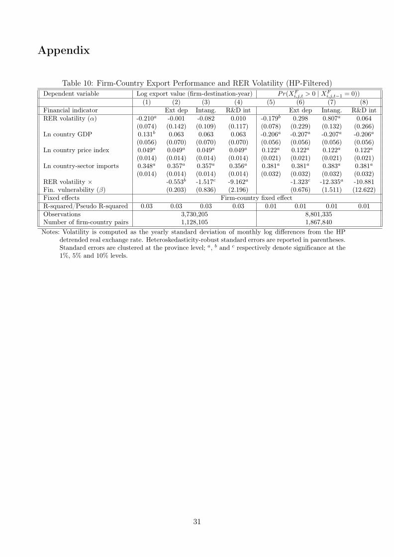
Appendix

Table 10: Firm-Country Export Performance and RER Volatility (HP-Filtered)Dependent variable Log export value (firm-destination-year) Pr(XF

i,j,t > 0 | XFi,j,t−1 = 0))

(1) (2) (3) (4) (5) (6) (7) (8)Financial indicator Ext dep Intang. R&D int Ext dep Intang. R&D intRER volatility (α) -0.210a -0.001 -0.082 0.010 -0.179b 0.298 0.807a 0.064

(0.074) (0.142) (0.109) (0.117) (0.078) (0.229) (0.132) (0.266)Ln country GDP 0.131b 0.063 0.063 0.063 -0.206a -0.207a -0.207a -0.206a

(0.056) (0.070) (0.070) (0.070) (0.056) (0.056) (0.056) (0.056)Ln country price index 0.049a 0.049a 0.049a 0.049a 0.122a 0.122a 0.122a 0.122a

(0.014) (0.014) (0.014) (0.014) (0.021) (0.021) (0.021) (0.021)Ln country-sector imports 0.348a 0.357a 0.357a 0.356a 0.381a 0.381a 0.383a 0.381a

(0.014) (0.014) (0.014) (0.014) (0.032) (0.032) (0.032) (0.032)RER volatility × -0.553b -1.517c -9.162a -1.323c -12.335a -10.881Fin. vulnerability (β) (0.203) (0.836) (2.196) (0.676) (1.511) (12.622)Fixed effects Firm-country fixed effectR-squared/Pseudo R-squared 0.03 0.03 0.03 0.03 0.01 0.01 0.01 0.01Observations 3,730,205 8,801,335Number of firm-country pairs 1,128,105 1,867,840Notes: Volatility is computed as the yearly standard deviation of monthly log differences from the HP

detrended real exchange rate. Heteroskedasticity-robust standard errors are reported in parentheses.Standard errors are clustered at the province level; a, b and c respectively denote significance at the1%, 5% and 10% levels.

31

Table11

:Firm-C

ountry

Exp

ortPerform

ance

andRER

Volatility:Alterna

tive

Indicatorof

IntensiveMargin

Dep

endent

variab

leLo

gaverageexpo

rtvalue(firm

-dest.-year)=totale

xp.value/Nbof

exp.

prod

.(1)

(2)

(3)

(4)

(5)

(6)

(7)

(8)

Finan

cial

indicator

Ext

dep

Intang

.R&D

int

Externa

ldep

endence

RER

volatility(α

)-0.198

a0.304c

0.095

0.167

0.329b

0.329b

0.237

0.220

(0.065)

(0.155)

(0.109)

(0.104)

(0.141)

(0.141)

(0.169)

(0.147)

Lncoun

tryGDP

-0.025

-0.025

-0.025

-0.025

-0.026

-0.026

-0.026

-0.025

(0.052)

(0.052)

(0.052)

(0.052)

(0.053)

(0.053)

(0.052)

(0.052)

Lncoun

trypriceindex

0.023c

0.023c

0.023c

0.023c

0.023c

0.023c

0.023c

0.023c

(0.012)

(0.012)

(0.012)

(0.012)

(0.012)

(0.012)

(0.012)

(0.012)

Lncoun

try-sector

impo

rts

0.290a

0.289a

0.290a

0.289a

0.289a

0.289a

0.289a

0.287a

(0.019)

(0.018)

(0.019)

(0.018)

(0.018)

(0.018)

(0.018)

(0.018)

RER

volatility×

Fin.vu

lnerab

ility

(β)

-1.349

a-3.890

a-14.796a

-1.837

a-1.849

a-1.215

b-1.137

a

(0.346)

(1.094)

(3.571)

(0.356)

(0.362)

(0.472)

(0.341)

RER

volatility×

Finan

cial

vulnerab

ility×

1.086a

Highfin

.devt

(abo

vemedian)

(0.170)

RER

volatility×

Finan

cial

vulnerab

ility×

1.109a

Highfin

.devt

(abo

vemean)

(0.177)

RER

volatility×

Finan

cial

vulnerab

ility×

6.061a

2.743a

Fin.devt

(δ)

(1.695)

(0.827)

RER

volatility×

Fin.de

vt(γ)

-1.780

a-0.543

c

(0.639)

(0.311)

Finan

cial

vulnerab

ility×

Fin.Devt

0.216c

(0.125)

Finan

cial

developm

ent

-0.004

-0.088

b

(0.023)

(0.035)

Fixed

effects

Firm-cou

ntry

fixed

effect

R-squ

ared

0.02

0.02

0.02

0.02

0.02

0.02

0.02

0.02

Observation

s3,731,351

Num

berof

firm-cou

ntry

pairs

1,128,873

Notes:H

eteroskeda

sticity-robu

ststan

dard

errors

arerepo

rted

inpa

rentheses.

Stan

dard

errors

areclusteredat

the

province

level;

a,b

and

crespectively

deno

tesign

ificanceat

the1%

,5%

and10%

levels.

32

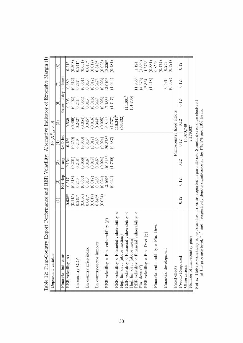
Table12

:Firm-C

ountry

Exp

ortPerform

ance

andRER

Volatility:Alterna

tive

Indicatorof

Extensive

Margin(I)

Dep

endent

variab

lePr(X

F i,j,t>

0)

(1)

(2)

(3)

(4)

(5)

(6)

(7)

(8)

Finan

cial

indicator

Ext

dep

Intang

.R&D

int

Externa

ldep

endence

RER

volatility(α

)-0.638

a0.517

0.154

-0.156

0.539

0.505

0.389

0.215

(0.115)

(0.318)

(0.201)

(0.250)

(0.409)

(0.402)

(0.312)

(0.308)

Lncoun

tryGDP

0.249a

0.249a

0.248a

0.249a

0.242a

0.241a

0.237a

0.241a

(0.056)

(0.056)

(0.056)

(0.056)

(0.054)

(0.054)

(0.051)

(0.051)

Lncoun

trypriceindex

0.045a

0.045a

0.046a

0.045a

0.045a

0.045a

0.045a

0.045a

(0.017)

(0.017)

(0.017)

(0.017)

(0.016)

(0.016)

(0.017)

(0.017)

Lncoun

try-sector

impo

rts

0.345a

0.345a

0.345a

0.345a

0.344a

0.344a

0.347a

0.343a

(0.024)

(0.024)

(0.024)

(0.024)

(0.025)

(0.025)

(0.023)

(0.023)

RER

volatility×

Fin.vu

lnerab

ility

(β)

-3.169

a-10.343a

-20.378a

-6.844

a-7.183

a-3.019

a-2.330

a

(0.624)

(1.700)

(6.387)

(1.737)

(1.747)

(1.044)

(0.481)

RER

volatility×

Finan

cial

vulnerab

ility×

110.241b

Highfin

.devt

(abo

vemedian)

(53.432)

RER

volatility×

Finan

cial

vulnerab

ility×

114.601b

Highfin

.devt

(abo

vemean)

(51.236)

RER

volatility×

Finan

cial

vulnerab

ility×

11.958

a1.124

Fin.devt

(δ)

(4.575)

(1.859)

RER

volatility×

Fin.Devt(γ)

-2.324

1.576c

(1.418)

(0.831)

Finan

cial

vulnerab

ility×

Fin.Devt

0.856c

(0.474)

Finan

cial

developm

ent

0.581

0.253

(0.367)

(0.321)

Fixed

effects

Firm-cou

ntry

fixed

effects

Pseud

oR-squ

ared

0.12

0.12

0.12

0.12

0.12

0.12

0.12

0.12

Observation

s15,070,749

Num

berof

firm-cou

ntry

pairs

2,179,037

Notes:Heteroskeda

sticity-robu

ststan

dard

errors

arerepo

rted

inpa

rentheses.

Stan

dard

errors

areclustered

attheprovince

level;

a,b

and

crespectively

deno

tesign

ificanceat

the1%

,5%

and10%

levels.

33

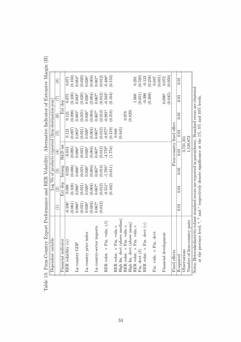
Table13

:Firm-C

ountry

Exp

ortPerform

ance

andRER

Volatility:Alterna

tive

Indicatorof

Extensive

Margin(II)

Dep

endent

variab

leLo

gNbof

prod

ucts

expo

rted

(firm

-destina

tion

-year)

(1)

(2)

(3)

(4)

(5)

(6)

(7)

(8)

Finan

cial

indicator

Ext

dep

Intang

.R&D

int

Ext

dep

RER

volatility(α

)-0.106

c0.098

0.029

-0.013

0.121

0.121

0.075

0.071

(0.061)

(0.108)

(0.086)

(0.095)

(0.097)

(0.098)

(0.100)

(0.103)

Lncoun

tryGDP

0.086a

0.086a

0.086a

0.086a

0.085a

0.085a

0.083a

0.084a

(0.021)

(0.021)

(0.021)

(0.021)

(0.021)

(0.021)

(0.020)

(0.020)

Lncoun

trypriceindex

0.026a

0.026a

0.026a

0.026a

0.026a

0.026a

0.026a

0.026a

(0.004)

(0.004)

(0.004)

(0.004)

(0.004)

(0.004)

(0.004)

(0.004)

Lncoun

try-sector

impo

rts

0.067a

0.067a

0.067a

0.067a

0.067a

0.067a

0.067a

0.067a

(0.012)

(0.012)

(0.012)

(0.012)

(0.012)

(0.012)

(0.012)

(0.012)

RER

volat.×

Fin.vu

ln.(β

)-0.551

a-1.795

a-3.778

b-0.977

a-0.991

a-0.503

a-0.486

a

(0.162)

(0.611)

(1.754)

(0.219)

(0.218)

(0.164)

(0.153)

RER

volat.×

Fin.vu

ln.×

0.948

Highfin

.devt

(abo

vemedian)

(0.845)

RER

volat.×

Fin.vu

ln.×

0.978

Highfin

.devt

(abo

vemean)

(0.829)

RER

volat.×

Fin.vu

ln.×

1.008

0.291

Fin.devt

(δ)

(0.651)

(0.520)

RER

volat.×

Fin.devt

(γ)

-0.390

-0.123

(0.269)

(0.256)

Fin.vu

ln.×

Fin.devt

0.047

(0.031)

Finan

cial

developm

ent

0.090c

0.072

(0.045)

(0.050)

Fixed

effects

Firm-cou

ntry

fixed

effect

R-squ

ared

0.01

0.01

0.01

0.01

0.01

0.01

0.01

0.01

Observation

s3,731,351

Num

berof

firm-cou

ntry

pairs

1,128,873

Notes:H

eteroskeda

sticity-robu

ststan

dard

errors

arerepo

rted

inpa

rentheses.

Stan

dard

errors

areclustered

attheprovince

level;

a,b

and

crespectively

deno

tesign

ificanceat

the1%

,5%

and10%

levels.

34

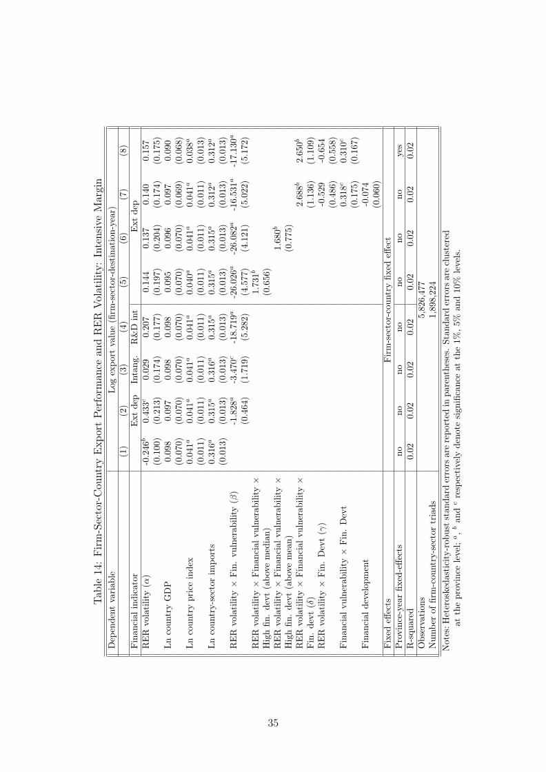
Table14

:Firm-Sector-Cou

ntry

Exp

ortPerform

ance

andRER

Volatility:IntensiveMargin

Dep

endent

variab

leLo

gexpo

rtvalue(firm

-sector-destination-year)

(1)

(2)

(3)

(4)

(5)

(6)

(7)

(8)

Finan

cial

indicator

Ext

dep

Intang

.R&D

int

Ext

dep

RER

volatility(α

)-0.246

b0.433c

0.029

0.207

0.144

0.137

0.140

0.157

(0.100)

(0.213)

(0.174)

(0.177)

(0.197)

(0.204)

(0.174)

(0.175)

Lncoun

tryGDP

0.098

0.097

0.098

0.098

0.095

0.096

0.097

0.090

(0.070)

(0.070)

(0.070)

(0.070)

(0.070)

(0.070)

(0.069)

(0.068)

Lncoun

trypriceindex

0.041a

0.041a

0.041a

0.041a

0.040a

0.041a

0.041a

0.038a

(0.011)

(0.011)

(0.011)

(0.011)

(0.011)

(0.011)

(0.011)

(0.013)

Lncoun

try-sector

impo

rts

0.316a

0.315a

0.316a

0.315a

0.315a

0.315a

0.312a

0.312a

(0.013)

(0.013)

(0.013)

(0.013)

(0.013)

(0.013)

(0.013)

(0.013)

RER

volatility×

Fin.vu

lnerab

ility

(β)

-1.828

a-3.470

c-18.719a

-26.026a

-26.082a

-16.531a

-17.130a

(0.464)

(1.719)

(5.282)

(4.577)

(4.121)

(5.022)

(5.172)

RER

volatility×

Finan

cial

vulnerab

ility×

1.731b

Highfin

.devt

(abo

vemed

ian)

(0.656)

RER

volatility×

Finan

cial

vulnerab

ility×

1.680b

Highfin

.devt

(abo

vemean)

(0.775)

RER

volatility×

Finan

cial

vulnerab

ility×

2.688b

2.650b

Fin.de

vt(δ)

(1.136)

(1.109)

RER

volatility×

Fin.Devt(γ)

-0.529

-0.654

(0.486)

(0.558)

Finan

cial

vulnerab

ility×

Fin.Devt

0.318c

0.310c

(0.175)

(0.167)

Finan

cial

developm

ent

-0.074

(0.060)

Fixed

effects

Firm-sector-coun

tryfix

edeff

ect

Province-year

fixed-effe

cts

nono

nono

nono

noyes

R-squ

ared

0.02

0.02

0.02

0.02

0.02

0.02

0.02

0.02

Observation

s5,826,477

Num

berof

firm-cou

ntry-sectortriads

1,898,224

Notes:H

eteroskeda

sticity-robu

ststan

dard

errors

arerepo

rted

inpa

rentheses.

Stan

dard

errors

areclustered

attheprovince

level;

a,b

and

crespectively

deno

tesign

ificanceat

the1%

,5%

and10%

levels.

35

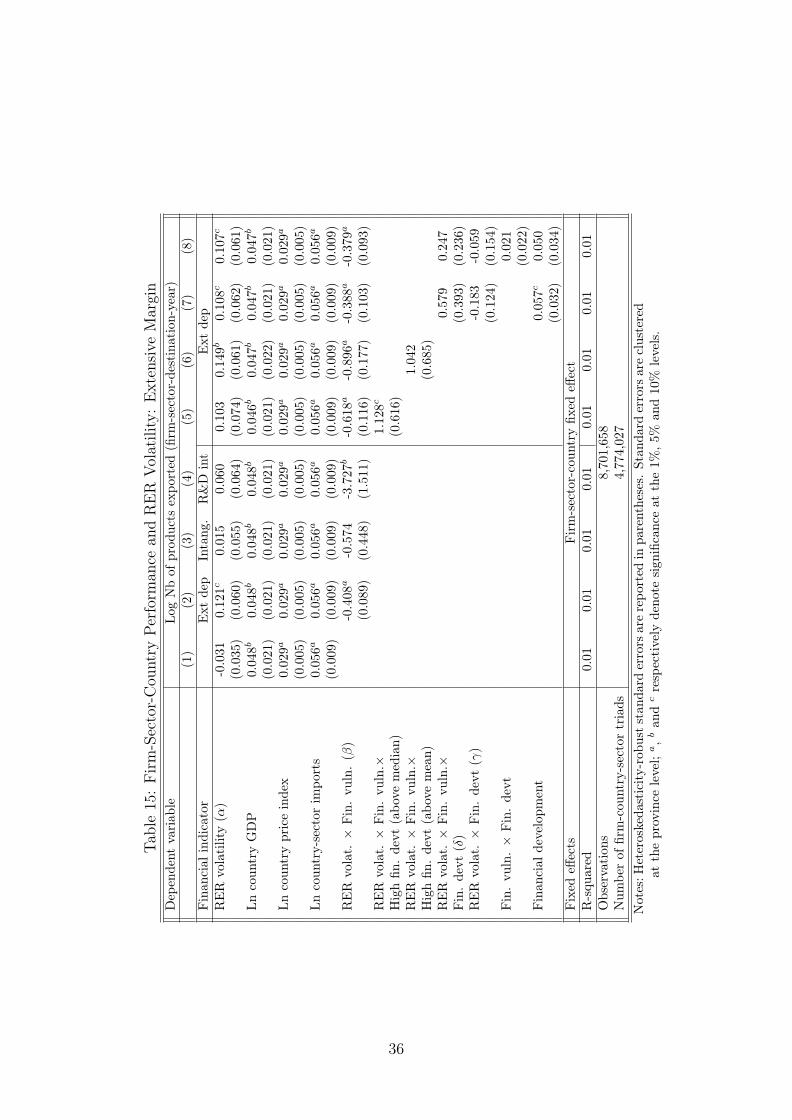
Table15

:Firm-Sector-Cou

ntry

Perform

ance

andRER

Volatility:Extensive

Margin

Dep

endent

variab

leLo

gNbof

prod

ucts

expo

rted

(firm

-sector-destination-year)

(1)

(2)

(3)

(4)

(5)

(6)

(7)

(8)

Finan

cial

indicator

Ext

dep

Intang

.R&D

int

Ext

dep

RER

volatility(α

)-0.031

0.121c

0.015

0.060

0.103

0.149b

0.108c

0.107c

(0.035)

(0.060)

(0.055)

(0.064)

(0.074)

(0.061)

(0.062)

(0.061)

Lncoun

tryGDP

0.048b

0.048b

0.048b

0.048b

0.046b

0.047b

0.047b

0.047b

(0.021)

(0.021)

(0.021)

(0.021)

(0.021)

(0.022)

(0.021)

(0.021)

Lncoun

trypriceindex

0.029a

0.029a

0.029a

0.029a

0.029a

0.029a

0.029a

0.029a

(0.005)

(0.005)

(0.005)

(0.005)

(0.005)

(0.005)

(0.005)

(0.005)

Lncoun

try-sector

impo

rts

0.056a

0.056a

0.056a

0.056a

0.056a

0.056a

0.056a

0.056a

(0.009)

(0.009)

(0.009)

(0.009)

(0.009)

(0.009)

(0.009)

(0.009)

RER

volat.×

Fin.vu

ln.(β

)-0.408

a-0.574

-3.727

b-0.618

a-0.896

a-0.388

a-0.379

a

(0.089)

(0.448)

(1.511)

(0.116)

(0.177)

(0.103)

(0.093)

RER

volat.×

Fin.vu

ln.×

1.128c

Highfin

.devt

(abo

vemedian)

(0.616)

RER

volat.×

Fin.vu

ln.×

1.042

Highfin

.devt

(abo

vemean)

(0.685)

RER

volat.×

Fin.vu

ln.×

0.579

0.247

Fin.devt

(δ)

(0.393)

(0.236)

RER

volat.×

Fin.devt

(γ)

-0.183

-0.059

(0.124)

(0.154)

Fin.vu

ln.×

Fin.devt

0.021

(0.022)

Finan

cial

developm

ent

0.057c

0.050

(0.032)

(0.034)

Fixed

effects

Firm-sector-coun

tryfix

edeff

ect

R-squ

ared

0.01

0.01

0.01

0.01

0.01

0.01

0.01

0.01

Observation

s8,701,658

Num

berof

firm-cou

ntry-sectortriads

4,774,027

Notes:H

eteroskeda

sticity-robu

ststan

dard

errors

arerepo

rted

inpa

rentheses.

Stan

dard

errors

areclustered

attheprov

ince

level;

a,b

and

crespectively

deno

tesign

ificanceat

the1%

,5%

and10%

levels.

36