Embed Size (px)
Citation preview

The information content of implied volatility in light
of the jump/continuous decomposition of realized
volatility
Pierre Giot and Sebastien Laurent∗
January 16, 2006
ABSTRACT
In the framework of encompassing regressions, we assess the information content
of the jump/continuous components of historical volatility when implied volatility is in-
cluded as an additional regressor. Our empirical application focuses on daily and in-
tradaily data for the S&P100 and S&P500 indexes, and daily data for the associated VXO
and VIX implied volatility indexes. Our results show that the total explanatory power
of the encompassing regressions barely changes when the jump/continuous components
are included, although the weekly and monthly continuous components are usually sig-
nificant. In contrast, the jump components of realized volatility are much less relevant,
although the monthly jump component sometimes does convey information. This evi-
∗Pierre Giot is a Professor of Finance at the Department of Business Administration & CEREFIM atUniversity of Namur, Rempart de la Vierge, 8, 5000 Namur, Belgium, Phone: +32 (0) 81 724887, Email:[email protected], and Center for Operations Research and Econometrics (CORE) at Universite catholiquede Louvain, Belgium. Sebastien Laurent is a Professor of Econometrics at the Department of Economics &CEREFIM at University of Namur, Rempart de la Vierge, 8, 5000 Namur, Belgium, Phone: +32 (0) 81 724887,Email: [email protected], and Center for Operations Research and Econometrics (CORE) at Uni-versite catholique de Louvain, Belgium.

dence supports the view that implied volatility has a very high information content, even
when extended decompositions of past realized volatility are used.
2

1. Introduction
The information content of implied volatility has been well documented in many empirical
studies. Most papers look at whether implied volatility helps predict future volatility by es-
timating either encompassing regressions or ARCH-type models. In both settings, volatility
forecasts are initially based on historical volatility. When implied volatility is included, the
important research issues focus on whether it supplies additional information and whether the
historical volatility is still relevant, i.e. what is the additional information content of historical
volatility. As the focus of these studies is on implied volatility, the historical volatility that
is used is often a rather crude measure (lagged realized volatility in an encompassing regres-
sion, lagged squared error term in the ARCH framework). In contrast, we suggest that more
sophisticated measures of historical volatility should be taken into account when assessing
the information content of implied volatility. In this paper, we use the recent continuous/jump
decomposition of historical realized volatility suggested by Andersen, Bollerslev, and Diebold
(2003). This decomposition also paves the way for a ‘time structure’ (daily, weekly, monthly
decomposition) for each volatility component. The latter decompositions are motivated by
the recent Heterogeneous Autoregressive model of the Realized Volatility (HAR-RV) intro-
duced by Corsi (2003). Hence, we look at the information content of the continuous and jump
components of historical volatility in encompassing regressions which also feature implied
volatility as an additional regressor. Our contribution to the literature is thus to provide a more
sophisticated and promising econometric framework to shed light on the information con-
tent of implied volatility when the latter is competing against extended measures of historical
volatility computed by market participants.
The empirical application focuses on the S&P100 and S&P500 indexes and associated
VXO and VIX implied volatility indexes. Our results show that the weekly and monthly con-
tinuous components of historical volatility convey information beyond the implied volatility
forecasts. In other words, when the weekly/monthly components are included in the encom-
passing regressions there is a shift in explanatory power away from the implied volatility
2
measure towards the extended historical measures. However, the total explanatory power of
the regression barely increases (the modified R2 suggested by Andersen, Bollerslev, and Med-
dahi, 2002, hovers around 0.7). This suggests that the implied volatility does indeed subsume
most relevant volatility information and also indicates that the extended decomposition of the
past historical volatility does not really help deliver better volatility forecasts. Jump com-
ponents provide much less information, although the monthly jump component of historical
volatility is sometimes significantly negative. This could suggest that agents tend to overreact
to sustained periods of ‘jump volatility’.
The rest of the paper is structured as follows. After this introduction, we characterize
the implied volatility and the continuous/jump components of realized volatility in Section 2.
Section 3 presents the econometric framework and the finance interpretation of the suggested
encompassing regressions. Section 4 details the datasets and Section 5 provides the empirical
application. Finally, Section 6 concludes.
2. Implied and realized volatility
2.1. Implied volatility
The information content of implied volatility has been examined in many studies for the last
20 years. Most empirical studies assess the information content of implied volatility by either
estimating so-called encompassing regressions (e.g. Christensen and Prabhala, 1998; Corrado
and Miller, 2004), or by estimating ARCH-type models with the lagged implied volatility in-
cluded as an additional variable in the conditional variance specification (e.g. Day and Lewis,
1992; Blair, Poon, and Taylor, 2001), or by looking at the added value of the implied volatility
in a finance application (e.g. Giot, 2005a, 2005b). Our contribution relies on encompassing
regressions that take into account the continuous/jump decomposition of the so-called realized
volatility introduced by Andersen and Bollerslev (1998b). Without this decomposition, the en-
3
compassing regression usually regress the h-day observed realized volatility against the h-day
implied volatility forecast and lagged values of the dependent variable (this is the approach
commonly used in the literature). The extended regressions that feature the continuous and
jump components of realized volatility are described in the next section.
While some authors use their own computation of implied volatility, others rely on the
availability of implied volatility indexes to derive h-day-ahead implied volatility forecasts.
This is also the chosen framework for the empirical application of the paper. In these latter
studies, the square root of time rule is used to switch from the ‘natural’ horizon of the implied
volatility index to the required h-day horizon. Our study focuses on the S&P100 and S&P500
indexes, for which the corresponding implied volatility indexes (VXO and VIX indexes) are
computed by the CBOE. The construction of the VXO index is described in Whaley (1993)
or Fleming and Whaley (1995). The new VIX index is detailed in the CBOE technical docu-
ment “The New CBOE Volatility Index - VIX” available from the CBOE website, or in Giot
(2005a). While we refer the reader to these papers for a detailed presentation of the construc-
tion of the implied volatility indexes, it is important to stress that the VXO and VIX indexes
are computed differently. Indeed, the VXO is based on the ‘old VIX’ formula, i.e. it is an
implied volatility backed out from 8 at-the-money options on the S&P100 index. In contrast,
the VIX index is computed from options on the S&P500 index and the options taken into
account feature a wide strike price variation. Consequently, the VIX should better integrate
the volatility information contained in the option prices, i.e. not only at-the-money options
but also options for which the strike price can be far away from the price of the index. For
both implied volatility indexes, their natural h-day-ahead horizon is equal to 22 trading days
(by construction), i.e. they are meant to deliver 22-day-ahead volatility forecasts for the un-
derlying stock index. As mentioned above, the square root of time rule is then used to switch
to another time horizon: given V XOt or V IXt available at the end of day t and expressed in
annualized terms, the h-day-ahead implied volatility forecast is equal to√
h365 V XOt for the
S&P100 index, while it is√
h365 V IXt for the S&P500 index.
4

2.2. Realized volatility and its two components
The recent widespread availability of databases providing the intraday prices of financial as-
sets (stocks, stock indexes, bonds, currencies,. . . ) has led to new developments in applied
econometrics and quantitative finance. The notion of realized volatility has been introduced
in the literature by Andersen and Bollerslev (1998b). The most interesting feature of realized
volatility is that it provides, under certain conditions, a consistent nonparametric estimate of
the asset price variability.
Let us consider the following continuous-time jump diffusion process for the logarithmic
price of an asset p(t):
d p(t) = µ(t)dt +σ(t)dW (t)+κ(t)dq(t), t ∈ [0,T ], (1)
where µ(t) is a continuous locally bounded variation process, the volatility process σ(t) is
strictly positive, W (t) denotes a standard Brownian motion, dq(t) is a counting process with
dq(t) = 1 corresponding to a jump at time t and dq(t) = 0 otherwise and κ(t) refers to the size
of the corresponding jumps.
The return over the discrete interval [t−∆, t],∆ > 0, is then given by r(t,∆)≡ p(t)− p(t−∆). Following Andersen and Bollerslev (1998b), the daily realized volatility is computed
by summing the corresponding 1/∆ high-frequency intraday squared returns1, RVt+1(∆) ≡1/∆
∑j=1
r2t+ j·∆,∆. As emphasized by many authors, see Barndorff-Nielsen and Shephard (2002)
among others,
RVt+1(∆)→Z t+1
tσ2(s)ds+ ∑
t<s≤t+1κ2(s), (2)
as ∆→ 0. Equation (2) then implies that the realized volatility is a consistent estimate of the
integrated volatility in the absence of jumps.
1Without loss of generality 1/∆ is assumed to be an integer.
5

In an important contribution to the realized volatility literature, Barndorff-Nielsen and
Shephard (2003) show that, unlike the realized volatility, the so-called bi-power variation
measures constructed from the summation of appropriately scaled cross-products of adjacent
high-frequency absolute returns gives a consistent estimate of the integrated volatility in the
presence of jumps. More formally, following Barndorff-Nielsen and Shephard (2003, 2004,
2005), the standardized realized bi-power variation measure is defined as:
BVt+1(∆)≡ µ−11
1/∆
∑j=2|rt+ j·∆,∆||rt+( j−1)·∆,∆|, (3)
where µ1 ≡√
2/π. It follows that
BVt+1(∆)→Z t+1
tσ2(s)ds, (4)
as ∆→ 0. Consequently, the jump component is consistently measured by:
Jt+1(∆)≡max[RVt+1(∆)−BVt+1(∆),0]. (5)
In this framework, Andersen, Bollerslev, and Diebold (2003) propose an elegant and sim-
ple statistical procedure for testing the significance of the jumps. Their procedure requires
the computation of the standardized realized tri-power quarticity (a consistent estimate of the
integrated quarticityZ t+1
tσ2(s)ds):
T Qt+1(∆)≡ ∆−1µ−34/3
1/∆
∑j=3|rt+ j·∆,∆|4/3|rt+( j−1)·∆,∆|4/3|rt+( j−2)·∆,∆|4/3, (6)
where µ4/3 ≡ 22/3Γ(7/6)Γ(1/2)−1. Accordingly, a jump is said to be significant when
Zt+1(∆)≡ log(RVt+1(∆))− log(BVt+1(∆))√∆(µ−4
1 +2µ−21 −5)T Qt+1(∆)BVt+1(∆)−2
> Φα, (7)
6

where Φα is the α quantile of the standard normal distribution.2
3. Econometric framework
3.1. Notation and econometric models
In this section, we build on the previous characterization of implied volatility and realized
volatility to define the variables we are working with and introduce the encompassing regres-
sions. Let t be the index for the daily observations and h be the forward-looking horizon
(expressed in number of days). On a daily basis, the following variables are defined. RV 1t
is the daily realized volatility over the [t : t + 1] time horizon computed from the 20-minute
intradaily returns observed over the same period of time (we full characterize our datasets in
the next section). Like in Andersen, Bollerslev, Diebold, and Ebens (2001), the daily realized
volatility is computed as the sum of the squared intraday returns. Following Andersen, Boller-
slev, and Diebold (2003) and the discussion presented in Section 2.2, RV 1t is split into RC1
t and
RJ1t . RV h
t is the realized volatility over [t : t +h], computed by summing the RV it , for i = 1 . . .h.
IMPht is the implied volatility observed at the end of day t and scaled such that it forecasts the
next h-day volatility: IMPht =
√h
365 IMP1t , with IMP1
t =V IXt or IMP1t =V XOt depending on
the chosen underlying stock index.3 Given the decomposition of RV 1t into RC1
t and RJ1t , we
define RCdt = RC1
t , RJdt = RJ1
t , RCwt = (RC1
t + . . .+ RC1t−4)/5, RJw
t = (RJ1t + . . .+ RJ1
t−4)/5,
RCmt = (RC1
t + . . .+RC1t−21)/22 and RJm
t = (RJ1t + . . .+RJ1
t−21)/22. These latter variables are
easily interpreted as the daily, weekly and monthly continuous and jump components (of the
realized volatility) respectively. For example, RCwt is the continuous component of the weekly
2To ensure that the measurements of the continuous sample path variation and the jump component add upto the realized volatility, non-significant jumps are transferred to the continuous sample path variation BVt+1(∆).See Andersen, Bollerslev, and Diebold (2003) for more details.
3Note that the most simple assessment of the implied volatility forecast would thus be a regression of RV ht
against IMPht .
7

realized volatility ending on day t; RJmt is the jump component of the monthly realized volatil-
ity ending on day t.
By definition, IMPht and RV h
t are based on overlapping data when as h > 1. To estimate the
extended encompassing regressions, we need to define related variables in a non-overlapping
framework (this issue was first highlighted by Christensen and Prabhala, 1998). Let k be the
index for the non-overlapping observations (1 . . .K). The following variables are then defined.
{RV hk } is the subset of {RV h
t } such that 1 out of h observations is retrieved. IMPhk , RCd
k , RCwk ,
RCmk , RJd
k , RJwk and RJm
k are defined similarly. We stress that all variables are interpreted
exactly as above. Since RCmt and RJm
t are based on an aggregation of the last 22 days, RCmk
and RJmk are the only variables that are still based on overlapping data when h = 5 or h = 10
days (hence we shall use the Newey-West procedure when estimating the regressions). This
is however consistent with the procedures put forth by Corsi (2003). Finally, all variables
are transformed in logs, yielding lRV hk = ln(RV h
k ), lIMPhk = ln(IMPh
k ),. . . The use of the log
realized volatility (and other log variables) in the regressions below is recommended to ensure
that the probability density of the error term is close to the normal density (Giot and Laurent,
2004).
To assess the information content of implied volatility in the extended framework that
features the continuous/jump decomposition, we estimate the following models:
Model 1
lRV hk = β0 +β1lIMPh
k + εk; (8)
Model 2
lRV hk = β0 +β1lIMPh
k +δdlRCdk +δwlRCw
k +δmlRCmk +γdlRJd
k +γwlRJwk +γmlRJm
k +εk;
(9)
Model 3
lRV hk = β0 +β1lIMPh
k + γdlRJdk + γwlRJw
k + γmlRJmk + εk. (10)
8

Next to these specifications, we also assess whether these regressions exhibit heteroscedas-
ticity. We consider F tests where we include the jump/continuous components as explanatory
variables. Regarding model 3 for example, the heteroscedasticity specification is:
e2k = α0 +α1lIMPh
k +α2lRJdk +α3lRJw
k +α4lRJmk +νk (11)
with H0: α1 = 0 and α2 = 0 and α3 = 0 and α4 = 0.
3.2. Interpretation of the models
The interpretation of the regressions is as follows. Model 1 is the most simple forecasting
regression: the observed realized volatility is compared with the forecast derived from the im-
plied volatility. This type of regression and the hypothesis tests that follow (e.g. is H0: β0 = 0
and β1 = 1 not rejected?) have been well documented in the literature. Model 2 is the extended
encompassing regression that features the daily, weekly and monthly continuous/jump compo-
nents of the realized volatility. In contrast to the standard regressions previously estimated in
the literature (e.g. lRV hk = β0 +β1lIMPh
k +β2lRV hk−1 +εk), we therefore assess the importance
of the decomposition and ‘time-structure’ of historical volatility. For example, most studies
based on lRV hk = β0 + β1lIMPh
k + β2lRV hk−1 + εk usually conclude that β2 is not significant.
This specification is however very restrictive as it implies that agents only take into account
the lagged h-day realized volatility when forecasting the next h-day volatility in addition of
the implied volatility. The continous/jump decomposition also allows us to assess the role
played by highly volatile markets regarding the quality of the volatility forecasts. Indeed, it is
well known that economic agents rely on the continuous component of realized volatility to
forecast future volatility (see Andersen, Bollerslev, and Diebold, 2002). But what is the im-
pact of prolonged periods of jump volatility? It could be argued that agents tend to overreact
and wrongly extrapolate this heightened volatility into the future. Last, does implied volatil-
ity subsume all relevant information? If this is true, the continuous and jump components
9
should not be significative. Model 3 is a restrictive version of model 2 where the continuous
components are not included.
The heteroscedasticity tests can also be interpreted in a finance framework since it can be
conjectured that a sustained period of jump volatility will lead to a much larger uncertainty in
the forecasting performances of the encompassing regressions. In the same vein, Christensen
and Prabhala (1998) and more recently Corrado and Miller (2005) study the impact of the
‘errors-in-variables’ problem in the encompassing regressions. Corrado and Miller (2005)
suggest (although they do not call it the jump component of volatility) that volatility can also
be decomposed into a ‘fundamental’ volatility and a ‘random’ volatility. The latter leads to
the errors-in-variables problem. Our continuous/jump framework therefore also allows us to
test if the precision of the regressions is affected by one (or both) of the volatility components.
4. The datasets
For the underlying stock indexes, the intraday data is provided by Tick Data (S&P100 and
S&P500 cash indexes sampled at the 20-minute frequency; the data is linearly interpolated as
in Muller, Dacorogna, Olsen, Pictet, Schwarz, and Morgenegg, 1990, and Dacorogna, Muller,
Nagler, Olsen, and Pictet, 1993). Regarding the VXO and VIX implied volatility indexes, the
daily data is supplied by the CBOE. The time period is 1/2/1990 - 3/5/2003 for all indexes.
Log returns are then defined and the daily realized volatility RV 1t is computed as in Andersen
and Bollerslev (1998a). Next, we decompose RV 1t into its continuous and jump components,
RC1t and RJ1
t , and compute the daily, weekly and monthly continuous and jump components.
In agreement with recent empirical papers on this topic, the jump threshold, α in Equation 7,
is set equal to 0.9999 (note that we assess the dependence of our results on the α threshold
later in the text). Finally, we switch to non-overlapping data with h successively equal to 5,
10 and 22 trading days. At the end of this process, we thus have 6 datasets, each dataset
featuring the h-day realized volatility, 6 historical volatility variables and 1 implied volatility
10

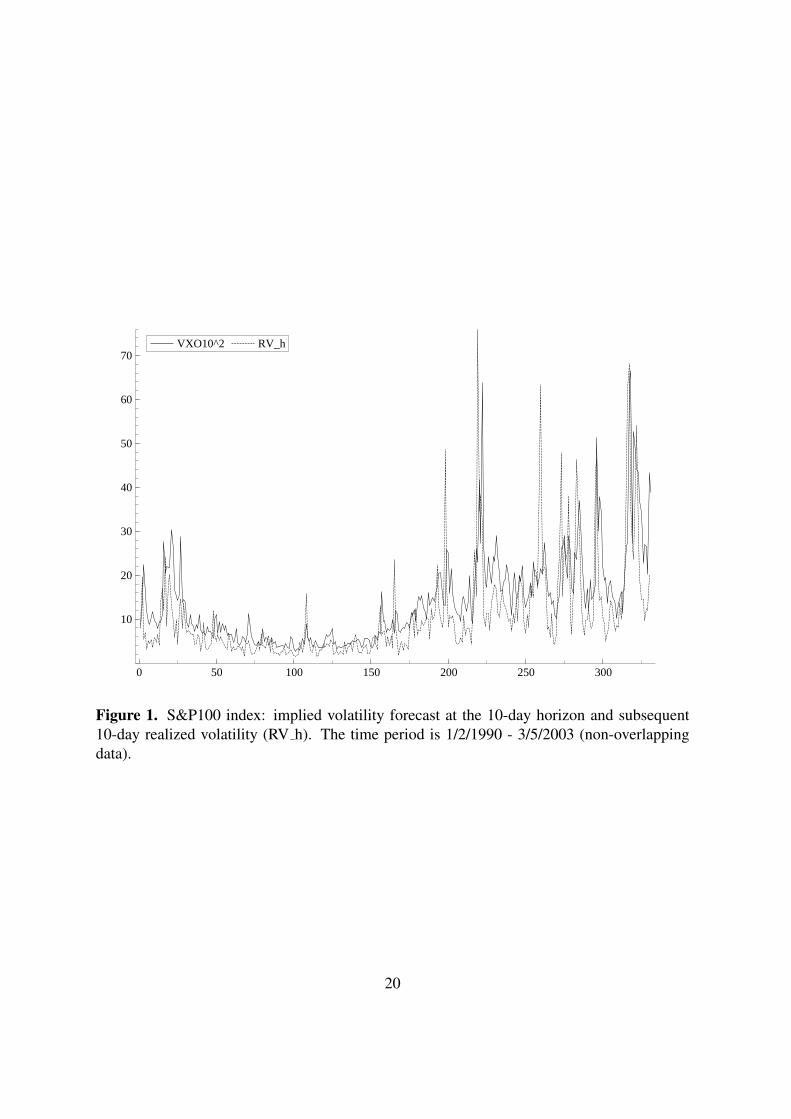
forecast. To illustrate the information content of implied volatility at the 10-day and 22-day
time horizons, we successively plot IMP10k vs RV 10
k and IMP22k vs RV 22
k for the two indexes in
Figures 1 to 4. As expected from the literature on implied volatility indexes, the fit between
the two series is very good, which bodes well for the assessment of the information content of
implied volatility in Model 1.
5. Empirical results
Empirical results for models 1 (M1 in the table), 2 (M2) and 3 (M3) are reported in Tables 1,
2 and 3 for h equal to 5, 10 and 22 days respectively. In each table, the left (right) panel is for
the S&P100 (S&P500) index. All regressions were estimated using the Newey-West option,
yielding autocorrelation consistent results. In each panel, below the estimated coefficients, we
also report the regressions R2 and adjusted R2 computed according to Andersen, Bollerslev,
and Meddahi (2002). Indeed, Andersen, Bollerslev, and Meddahi (2002) show that the usual
R2s should be modified when assessing volatility forecasts in a realized volatility framework.
They derive adjusted R2 measures that take the highlighted biases into account. We also give
the P-values for the heteroscedasticity test described in Section 3.1.
The empirical results are quite similar for the six datasets. Results for the most simple
model (M1) indicate that the β1 coefficient for the log implied volatility is almost equal to 1.
For five cases out of six, we do not reject this hypothesis at the conventional level of signif-
icance. Because the constant (β0) is however different from 0, we reject the null hypothesis
of unbiasedness (this is confirmed by a joint test on both coefficients). Nevertheless, the fact
that β1 is almost equal to 1 supports the hypothesis that implied volatility almost moves one-
to-one with future realized volatility. The large R2 and adjusted R2 values also indicate that
implied volatility has a high information content: for the three horizons, the explicative power
of implied volatility is close to 70%. Note that this number is remarkably stable, whatever the
time horizon (h) taken into account.
11

As far as model 2 is concerned, the inclusion of the continuous/jump components leads to
a sharp decrease in the β1 coefficient; correspondingly, the weekly and monthly continuous
components are significantly different from zero in almost all cases. In contrast, the jump com-
ponents are much less significant. Although the weekly and monthly continuous components
are significant in most cases, it is important to note that the R2 and adjusted R2 barely increase
when switching from model 1 to model 2. Indeed, for both indexes and three horizons, some
explicative power is transferred from the implied volatility to the continuous components but
the total explicative power of the encompassing regression hardly increases. These facts tend
to support the hypothesis that implied volatility has, by itself, a very high information content
and that past ‘extended’ measures of realized volatility do not really bring valuable additional
information.
Note that the coefficient for the monthly jump component is in some cases significantly
negative and takes a rather large negative value. We interpret this as evidence that sustained
periods of jump volatility lead to an overestimation of future realized volatility (either by the
implied volatility index and/or by the continuous component of historical volatility). This
is most likely due to agents overreacting to recent (but sustained) market conditions. Finally,
model 3 sheds some light on the behavior of the implied volatility index when used in conjunc-
tion with the jump components of historical volatility. In that latter case, the empirical results
(estimated coefficients for β0 and β1, R2 and adjusted R2) are very similar to those of Model
1. This supports the view that jump components do not bring forth valuable information (as
far as forecasting is concerned).
Quite surprisingly, the heteroscedasticity tests (P-values are given at the bottom of each
panel in the tables) show that the explanatory variables do not have any impact on the squared
error terms for all specifications but one. Indeed, the null hypothesis of no heteroscedasticity
is (almost) never rejected at the conventional 5% level. In light of the discussion at the end
of Section 3.2, the precision of the encompassing regressions does not seem to be affected
by the jump and continuous components of historical volatility. This result tends to support
12
the conclusions of Corrado and Miller (2005), who show that the errors-in-variables problem
hardly affects the encompassing regressions (although they do conclude that forecast errors
occurred much more frequently before 1994).
Additional estimation results To assess the robustness of our results, we implemented a
series of changes regarding the definition of our variables and specification of the regressions.
First, we looked at the impact of the jump component selection parameter. If this threshold is
decreased, fewer intraday movements are classified as jumps. Second, we estimated models 1,
2 and 3 using a slightly different HAR specification. Indeed, in the current HAR specification
of Corsi (2003), RCwt includes 1/5 of RCd
t , RCmt includes 1/22 of RCd
t ,. . . We introduced a
modified HAR specification such that RCwt = (RC1
t−1 + . . .+RC1t−4)/4, RCm
t = (RC1t−5 + . . .+
RC1t−21)/17,. . . In this modified setting, variables RCd
t , RCwt , RCm
t , RJdt , RJw
t and RJmt no longer
share volatility information. Third, we implemented rolling regressions for all models (fixed
3-year window length). The new empirical results were in line with those documented above
and allowed us to conclude similarly.
6. Conclusion
This paper looks at the information content of the jump and continuous components of histor-
ical volatility in encompassing regressions that feature implied volatility as a regressor (Chris-
tensen and Prabhala, 1998, framework). In contrast to previous empirical studies, we therefore
assess whether the continuous/jump decomposition of historical volatility and its time struc-
ture impact the explanatory power and information content of implied volatility.
Our empirical results for the S&P100 and S&P500 indexes show that the highlighted
weekly and monthly continuous components convey information beyond implied volatility.
In a few cases, the jump components are also significant. However, the total explanatory
power of the encompassing regressions barely changes when switching from the most simple
13

model (only implied volatility is included) to the most sophisticated model (implied volatil-
ity and the full time structure decomposition of the continuous and jump components). This
tends to support the fact that implied volatility does indeed subsume most relevant volatility
information, even when ‘extended’ decomposition of the historical volatility are used. Finally,
the precision of the regressions do not seem to be affected by either the continuous or jump
components of volatility.
References
Andersen, T.G., and T. Bollerslev, 1998a, Answering the skeptics: yes, standard volatility
models do provide accurate forecasts, International Economic Review 39, 885–905.
Andersen, T.G., and T. Bollerslev, 1998b, DM-dollar volatility: intraday activity patterns,
macroeconomic announcements, and longer-run dependencies, Journal of Finance 53,
219–265.
Andersen, T.G., T. Bollerslev, and F.X. Diebold, 2003, Some Like it Smooth, and
Some Like it Rough: Untangling Continuous and Jump Components in Measuring,
Modeling, and Forecasting Asset Return Volatility, PIER Working Paper No. 03-025.
http://ssrn.com/abstract=465282.
Andersen, T.G., T. Bollerslev, F.X. Diebold, and H. Ebens, 2001, The distribution of stock
return volatility, Journal of Financial Economics 61, 43–76.
Andersen, T.G., T. Bollerslev, and N. Meddahi, 2002, Correcting the errors: a note on volatil-
ity forecast evaluation based on high-frequency data and realized volatilities, CIRANO
Working Paper 2002s-91.
Barndorff-Nielsen, O.E., and N. Shephard, 2002, Econometric Analysis of Realised Volatil-
ity and its use in Estimating Stochastic Volatility Models, Journal of the Royal Statistical
Society 64, 253–280.
14

Barndorff-Nielsen, O.E., and N. Shephard, 2003, Realised Power Variation and Stochastic
Volatility, Bernoulli 9, 243–265.
Barndorff-Nielsen, O.E., and N. Shephard, 2004, Power and bipower variation with stochastic
volatility and jumps (with discussion), Journal of Financial Econometrics 2, 1–48.
Barndorff-Nielsen, O.E., and N. Shephard, 2005, Econometrics of testing for jumps in finan-
cial economics using bipower variation, forthcoming in Journal of Financial Econometrics.
Blair, B.J., S. Poon, and S.J. Taylor, 2001, Forecasting S&P100 volatility: the incremental
information content of implied volatilities and high-frequency index returns, Journal of
Econometrics 105, 5–26.
Christensen, B.J., and N.R. Prabhala, 1998, The relation between implied and realized volatil-
ity, Journal of Financial Economics 50, 125–150.
Corrado, C.J., and T.W. Miller, 2005, The forecast quality of CBOE implied volatility indexes,
Journal of Futures Markets 25, 339–373.
Corsi, F., 2003, A Simple Long Memory Model of Realized Volatility, Manuscript, University
of Southern Switzerland. http://ssrn.com/abstract=626064.
Dacorogna, M.M., U.A. Muller, R.J. Nagler, R.B. Olsen, and O.V. Pictet, 1993, A Geograph-
ical Model for the Daily and Weekly Seasonal Volatility in the Foreign Exchange Market,
Journal of International Money and Finance 12, 413–438.
Day, T.E., and C.M. Lewis, 1992, Stock market volatility and the information content of stock
index options, Journal of Econometrics 52, 267–287.
Fleming, J., Ostdiek B., and R.E. Whaley, 1995, Predicting stock market volatility: a new
measure, Journal of Futures Markets 15, 265–302.
Giot, P., 2005a, Implied volatility indexes and daily Value-at-Risk models, Journal of Deriva-
tives 12, 54–64.
Giot, P., 2005b, Relationships between implied volatility indexes and stock index returns,
Journal of Portfolio Management 31, 92–100.
15
Giot, P., and S. Laurent, 2004, Modelling daily Value-at-Risk using realized volatility and
ARCH type models, Journal of Empirical Finance 11, 379–398.
Muller, U.A., M.M. Dacorogna, R.B. Olsen, O.V. Pictet, M. Schwarz, and C. Morgenegg,
1990, Statistical Study of Foreign Exchange Rates, Empirical Evidence of a Price Change
Scaling Law, and Intraday Analysis, Journal of Banking and Finance 14, 1189–1208.
Whaley, R.E., 1993, Derivatives on market volatility: hedging tools long overdue, Journal of
Derivatives 1, 71–84.
16
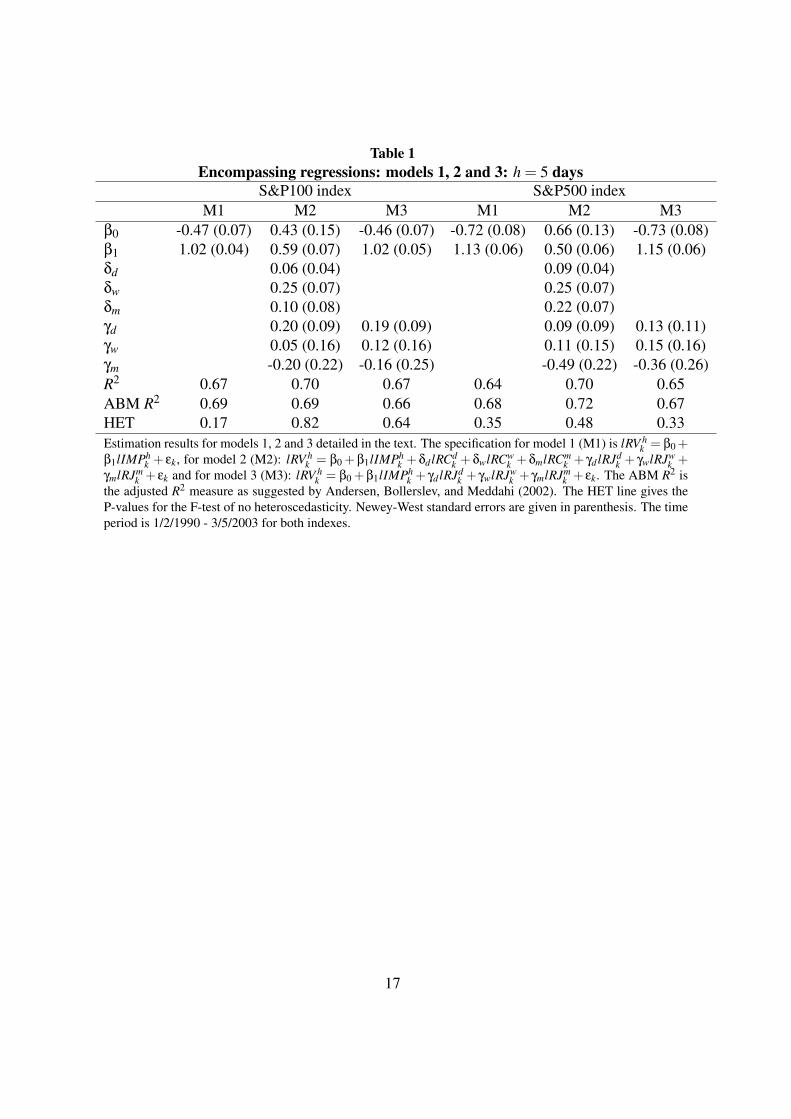
Table 1Encompassing regressions: models 1, 2 and 3: h = 5 days
S&P100 index S&P500 indexM1 M2 M3 M1 M2 M3
β0 -0.47 (0.07) 0.43 (0.15) -0.46 (0.07) -0.72 (0.08) 0.66 (0.13) -0.73 (0.08)β1 1.02 (0.04) 0.59 (0.07) 1.02 (0.05) 1.13 (0.06) 0.50 (0.06) 1.15 (0.06)δd 0.06 (0.04) 0.09 (0.04)δw 0.25 (0.07) 0.25 (0.07)δm 0.10 (0.08) 0.22 (0.07)γd 0.20 (0.09) 0.19 (0.09) 0.09 (0.09) 0.13 (0.11)γw 0.05 (0.16) 0.12 (0.16) 0.11 (0.15) 0.15 (0.16)γm -0.20 (0.22) -0.16 (0.25) -0.49 (0.22) -0.36 (0.26)R2 0.67 0.70 0.67 0.64 0.70 0.65ABM R2 0.69 0.69 0.66 0.68 0.72 0.67HET 0.17 0.82 0.64 0.35 0.48 0.33Estimation results for models 1, 2 and 3 detailed in the text. The specification for model 1 (M1) is lRV h
k = β0 +β1lIMPh
k + εk, for model 2 (M2): lRV hk = β0 + β1lIMPh
k + δd lRCdk + δwlRCw
k + δmlRCmk + γd lRJd
k + γwlRJwk +
γmlRJmk + εk and for model 3 (M3): lRV h
k = β0 +β1lIMPhk + γd lRJd
k + γwlRJwk + γmlRJm
k + εk. The ABM R2 isthe adjusted R2 measure as suggested by Andersen, Bollerslev, and Meddahi (2002). The HET line gives theP-values for the F-test of no heteroscedasticity. Newey-West standard errors are given in parenthesis. The timeperiod is 1/2/1990 - 3/5/2003 for both indexes.
17
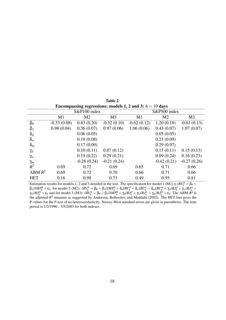
Table 2Encompassing regressions: models 1, 2 and 3: h = 10 days
S&P100 index S&P500 indexM1 M2 M3 M1 M2 M3
β0 -0.33 (0.08) 0.83 (0.20) -0.32 (0.10) -0.62 (0.12) 1.20 (0.18) -0.63 (0.13)β1 0.98 (0.04) 0.56 (0.07) 0.97 (0.06) 1.06 (0.06) 0.43 (0.07) 1.07 (0.07)δd 0.06 (0.05) 0.05 (0.05)δw 0.18 (0.08) 0.23 (0.09)δm 0.17 (0.09) 0.29 (0.07)γd 0.10 (0.11) 0.07 (0.12) 0.15 (0.11) 0.15 (0.13)γw 0.19 (0.22) 0.29 (0.21) 0.09 (0.24) 0.16 (0.23)γm -0.28 (0.24) -0.21 (0.24) -0.42 (0.21) -0.27 (0.26)R2 0.69 0.72 0.69 0.65 0.71 0.66ABM R2 0.69 0.72 0.70 0.66 0.71 0.66HET 0.16 0.98 0.73 0.49 0.95 0.81Estimation results for models 1, 2 and 3 detailed in the text. The specification for model 1 (M1) is lRV h
k = β0 +β1lIMPh
k + εk, for model 2 (M2): lRV hk = β0 + β1lIMPh
k + δd lRCdk + δwlRCw
k + δmlRCmk + γd lRJd
k + γwlRJwk +
γmlRJmk + εk and for model 3 (M3): lRV h
k = β0 +β1lIMPhk + γd lRJd
k + γwlRJwk + γmlRJm
k + εk. The ABM R2 isthe adjusted R2 measure as suggested by Andersen, Bollerslev, and Meddahi (2002). The HET line gives theP-values for the F-test of no heteroscedasticity. Newey-West standard errors are given in parenthesis. The timeperiod is 1/2/1990 - 3/5/2003 for both indexes.
18
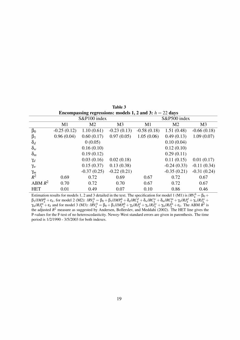
Table 3Encompassing regressions: models 1, 2 and 3: h = 22 days
S&P100 index S&P500 indexM1 M2 M3 M1 M2 M3
β0 -0.25 (0.12) 1.10 (0.61) -0.23 (0.13) -0.58 (0.18) 1.51 (0.48) -0.66 (0.18)β1 0.96 (0.04) 0.60 (0.17) 0.97 (0.05) 1.05 (0.06) 0.49 (0.13) 1.09 (0.07)δd 0 (0.05) 0.10 (0.04)δw 0.16 (0.10) 0.12 (0.10)δm 0.19 (0.12) 0.29 (0.11)γd 0.03 (0.16) 0.02 (0.18) 0.11 (0.15) 0.01 (0.17)γw 0.15 (0.37) 0.13 (0.38) -0.24 (0.33) -0.11 (0.34)γm -0.37 (0.25) -0.22 (0.21) -0.35 (0.21) -0.31 (0.24)R2 0.69 0.72 0.69 0.67 0.72 0.67ABM R2 0.70 0.72 0.70 0.67 0.72 0.67HET 0.01 0.49 0.07 0.10 0.86 0.46Estimation results for models 1, 2 and 3 detailed in the text. The specification for model 1 (M1) is lRV h
k = β0 +β1lIMPh
k + εk, for model 2 (M2): lRV hk = β0 + β1lIMPh
k + δd lRCdk + δwlRCw
k + δmlRCmk + γd lRJd
k + γwlRJwk +
γmlRJmk + εk and for model 3 (M3): lRV h
k = β0 +β1lIMPhk + γd lRJd
k + γwlRJwk + γmlRJm
k + εk. The ABM R2 isthe adjusted R2 measure as suggested by Andersen, Bollerslev, and Meddahi (2002). The HET line gives theP-values for the F-test of no heteroscedasticity. Newey-West standard errors are given in parenthesis. The timeperiod is 1/2/1990 - 3/5/2003 for both indexes.
19
0 50 100 150 200 250 300
10
20
30
40
50
60
70VXO10^2 RV_h
Figure 1. S&P100 index: implied volatility forecast at the 10-day horizon and subsequent10-day realized volatility (RV h). The time period is 1/2/1990 - 3/5/2003 (non-overlappingdata).
20

0 20 40 60 80 100 120 140
20
40
60
80
100
120
140 VXO22^2 RV_h
Figure 2. S&P100 index: implied volatility forecast at the 22-day horizon and subsequent22-day realized volatility (RV h). The time period is 1/2/1990 - 3/5/2003 (non-overlappingdata).
21

0 50 100 150 200 250 300
10
20
30
40
50
60
70VIX10^2 RV_h
Figure 3. S&P500 index: implied volatility forecast at the 10-day horizon and subsequent10-day realized volatility (RV h). The time period is 1/2/1990 - 3/5/2003 (non-overlappingdata).
22

0 20 40 60 80 100 120 140
20
40
60
80
100
120
VIX22^2 RV_h
Figure 4. S&P500 index: implied volatility forecast at the 22-day horizon and subsequent22-day realized volatility (RV h). The time period is 1/2/1990 - 3/5/2003 (non-overlappingdata).
23