Embed Size (px)
Citation preview
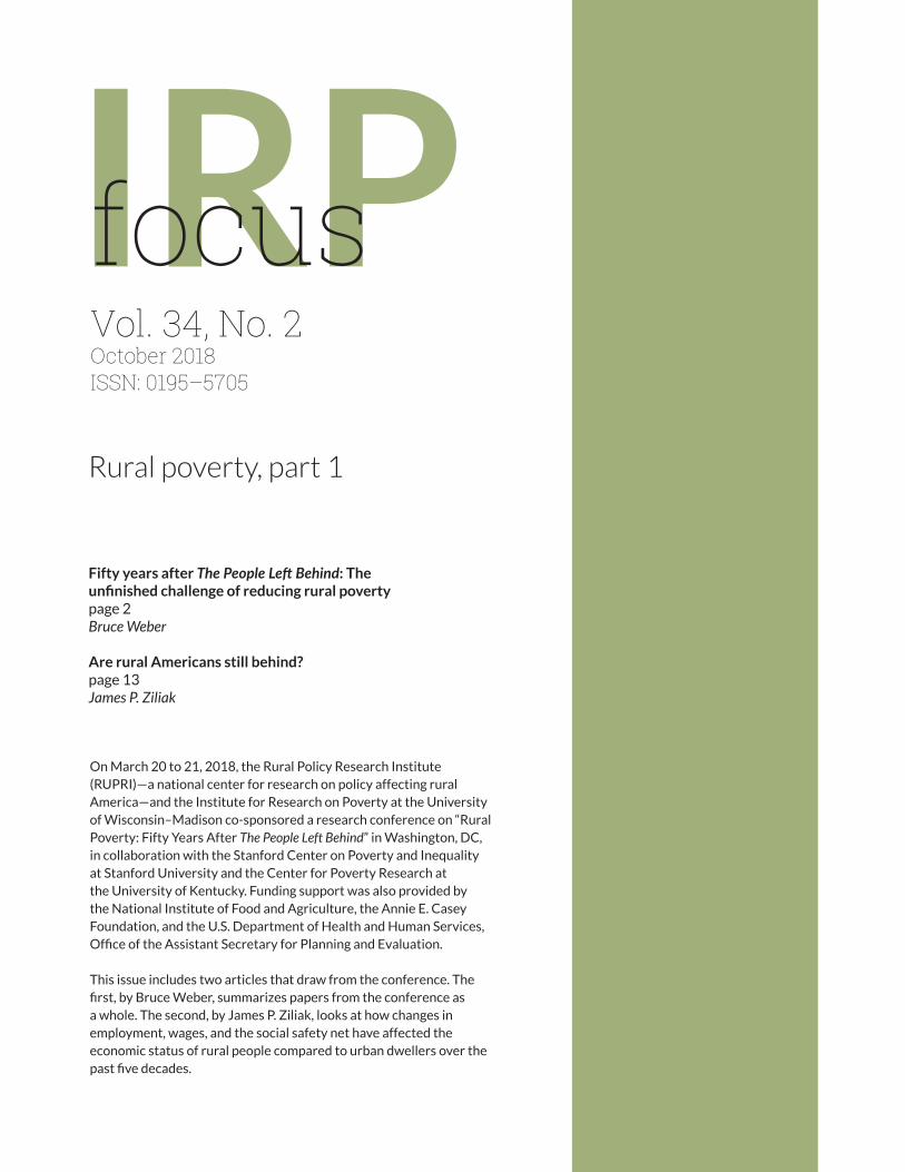
IRPfocus Vol. 34, No. 2October 2018 ISSN: 0195–5705
Fifty years after The People Left Behind: The unfinished challenge of reducing rural povertypage 2Bruce Weber
Are rural Americans still behind?page 13James P. Ziliak
Rural poverty, part 1
On March 20 to 21, 2018, the Rural Policy Research Institute (RUPRI)—a national center for research on policy affecting rural America—and the Institute for Research on Poverty at the University of Wisconsin–Madison co-sponsored a research conference on “Rural Poverty: Fifty Years After The People Left Behind” in Washington, DC, in collaboration with the Stanford Center on Poverty and Inequality at Stanford University and the Center for Poverty Research at the University of Kentucky. Funding support was also provided by the National Institute of Food and Agriculture, the Annie E. Casey Foundation, and the U.S. Department of Health and Human Services, Office of the Assistant Secretary for Planning and Evaluation.
This issue includes two articles that draw from the conference. The first, by Bruce Weber, summarizes papers from the conference as a whole. The second, by James P. Ziliak, looks at how changes in employment, wages, and the social safety net have affected the economic status of rural people compared to urban dwellers over the past five decades.

Focus, 2
IRP | focus vol. 34 no. 2 | 10.2018
Focus is the flagship publication of the Institute for Research on Poverty.
1180 Observatory Drive 3412 Social Science Building University of Wisconsin–Madison Madison, Wisconsin 53706 (608) 262-6358
The Institute for Research on Poverty (IRP) is a nonprofit, nonpartisan, university-based research center. As such, it takes no stand on public policy issues. Any opinions expressed in its publications are those of the authors and should not be construed as representing the opinions of IRP.
Focus is free of charge and distills poverty research of interest for dissemination to a broader audience, with a specific focus on educators, policymakers, policy analysts, and state and federal officials.
Edited by Emma Caspar.
For permission to reproduce Focus articles, please send your requests to [email protected].
Copyright © 2018 by the Regents of the University of Wisconsin System on behalf of the Institute for Research on Poverty. All rights reserved.
This publication was supported by Cooperative Agreement number AE000103 from the U.S. Department of Health and Human Services, Office of the Assistant Secretary for Planning and Evaluation to the Institute for Research on Poverty at the University of Wisconsin–Madison. The opinions and conclusions expressed herein are solely those of the author(s) and should not be construed as representing the opinions or policy of any agency of the Federal government.
Focus, 3
IRP | focus vol. 34 no. 2 | 10.2018
irp.wisc.edu | [email protected]
IRPfocus
Fifty years after The People Left Behind: The unfinished challenge of reducing rural povertyBruce Weber
Bruce Weber is Emeritus Professor of Applied Economics at Oregon State University.
October 2018 | Vol. 34, No. 2
The “Rural Poverty: Fifty Years After The People Left Behind” conference brought over 100 researchers and policymakers together for two days to review lessons learned about the causes and consequences of rural poverty and to provide a baseline for developing a research agenda aimed at improving economic opportunity and the well-being of low-income people in rural communities. Conference participants included established and emerging scholars from universities, government agencies, and nonprofits as well as leaders in government, advocacy organizations, and foundations.
The People Left Behind reportPresident Lyndon Johnson convened the National Advisory Commission on Rural Poverty to focus the nation’s attention on the plight of the rural poor. He charged the Commission “to make a comprehensive study and appraisal of the current economic situations and trends, as they relate to the existence of income and community problems in rural areas,” and to evaluate current programs and “develop recommendations for action by local, state, and federal governments and private enterprise as to the most efficient and promising means of providing opportunities for the rural population to share in America’s abundance.”1
In September 1967, the Commission released their findings in The People Left Behind report. In the report, the Commission reminded policymakers that rural people were at much higher risk of poverty than urban residents. At the time, the rural poverty rate was 25 percent, almost twice the urban rate. The Commission also noted wide geographic disparities in poverty rates, and pockets of rural poverty in the South, in Appalachia, and in the Southwest.
The report was developed in an era in which policymakers believed the nation had the resources and duty to eliminate poverty, and the Commission believed that “abolition of rural poverty… is completely feasible.”2 The report contained 12 chapters in which the Commission provided 12 sets of recommendations for policies it felt were needed to abolish rural poverty. The first task identified as necessary was “creating a favorable economic environment” (full employment, guaranteed employment, minimum wage, and ending racial and locational discrimination). The report then included five chapters on investments in people (manpower programs, education, health and medical care, family planning, and safety net programs); four chapters on investments in places (rural housing, area and regional development, community organizations, and natural resource and conservation projects; and two chapters on redesigning institutions (updating farm and natural resource policy to benefit poor residents, and changes in local, state and federal government administration).
Since The People Left Behind was written, the social and economic context of poverty and the reach of the social safety net have changed in fundamental ways. First, the level of income
Analysis that provides links both across rural and urban places and across national boundaries is needed.
Since poverty is primarily an income issue, promising rural antipoverty policies include public employment for low-skilled workers in need of employment.
More research is needed on the types of training programs that will help low-skilled workers to obtain employment.

Focus, 4
IRP | focus vol. 34 no. 2 | 10.2018
inequality has surged since 1970, deeply dividing the United States into a prosperous upper quintile (and an even more privileged top 1 percent) that has benefited from the growth in the economy, and the rest of the population that has not shared in this growth to any appreciable extent. Second, the safety net developed during and after the War on Poverty to help the least advantaged in this society has changed over the past 20 years in ways that have kept the poverty rate relatively stable, but that have also provided a smaller share of its benefits to those who are in deep poverty (incomes less than half the poverty line).
The March 2018 conference marking the fiftieth anniversary of The People Left Behind provided an opportunity to focus the attention of rural and urban stakeholders, policymakers, and academics on the high current levels of rural poverty; on what has been learned about policies, programs, and strategies that work to reduce rural poverty; and on knowledge gaps needing to be filled. The conference was structured around four themes of rural life:
• how race affects poverty, underemployment, and income mobility;
• child poverty and local strategies for addressing childhood disadvantage;
• how economic restructuring and entrepreneurial activity are related to poverty and mortality; and
• the social safety net and poverty dynamics.
This article summarizes the three invited presentations that reviewed major demographic, economic, and policy changes since the 1960s, and the 12 papers that address these four themes.
The People Left Behind: An unfinished legacyBruce Weber and Tracey Farrigan (U.S. Department of Agriculture Economic Research Service geographer) opened the conference with an overview of The People Left Behind and the geography of economic distress used in the report to highlight how little the geography of poverty has changed in the United States over the past 50 years. They noted some unique features of The People Left Behind. It was the first significant federal effort to call attention to the problem of nonfarm rural poverty. And the report recommended not just new programs that made investments in rural people and places, but it rather boldly advocated changes in underlying social institutions (racial discrimination) and economic rights (guaranteed employment—“a job for every rural person willing and able to work”). The report also underscored links with urban poverty, asserting that “it is impossible to obliterate urban poverty without removing its rural causes.” Compared to later research that defined poverty solely in terms of income inadequacy, this report focused on the broad dimensions of poverty (including lack of respect, agency,
Defining “urban” and “rural”Note that determining which areas are urban and which are rural is challenging. The Current Population Survey (CPS) and federal data sources that use counties as their base geography do not permit identification of “urban” and “rural” areas. Instead, counties are divided into only “metro” and “nonmetro,” where each metro area must contain either a place with a minimum population of 50,000, or a Census Bureau-defined urbanized area and a total population of at least 100,000 (75,000 in New England). In this article, metro areas are called “urban” and nonmetro areas are called “rural.” While this is not a perfect match, it is the best possible given available data.
Measuring povertyThe U.S. Census Bureau uses two primary poverty measures—the official poverty measure (OPM) and the Supplemental Poverty Measure (SPM). For each the Census Bureau calculates the poverty rate by comparing a measure of resources to the established poverty threshold.
OPM poverty thresholds are calculated as three times the cost of a nutritionally adequate diet in 1964, adjusted for inflation and family size. Resources are calculated as pre-tax cash income.
SPM thresholds are based on expenditures on food, clothing, shelter, and utilities, with adjustments for family size and composition, and for geographic differences in housing costs. Resources are measured as post-tax post-transfer cash income, counting tax credits and near-cash in-kind benefits such as the Supplemental Nutrition Assistance Program (SNAP) and housing assistance. Non-discretionary expenditures such as medical out-of-pocket costs, childcare, work expenses, and child support paid to another house hold are subtracted.
To learn more about the official poverty measures and alternative measures, see: https://www.irp.wisc.edu/resources/how-is-poverty-measured/
Focus, 5
IRP | focus vol. 34 no. 2 | 10.2018
and security). It characterized the economic status of rural Americans using a five-factor index based on measures of income, housing inadequacy, low educational attainment, and a “dependency ratio” of the number of children and elderly divided by the working age population. Noteworthy in the report were both the sense of optimism about prospects for reducing poverty and the sense of urgency for implementing their recommendations.
In assessing changes in the geography of poverty, Farrigan and her colleagues noted that while there are rural places that continue to be left behind, the overall economic status of rural populations has increased greatly since the 1960s, and that failing to account for changes in rural-to-urban designation masks improvement in rural conditions.3
The changing demographic, economic, and policy context since The People Left Behind
This introduction was followed by two invited presentations that reviewed the economic, demographic, and policy changes over the past half century that have affected the nation’s progress in reducing rural poverty. These retrospective papers focused on “lessons learned” about the causes and consequences of rural poverty and the effectiveness of poverty-reducing policies and programs.
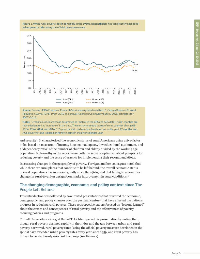
Cornell University sociologist Daniel T. Lichter opened his presentation by noting that, though rural poverty declined rapidly in the 1960s and the gap between urban and rural poverty narrowed, rural poverty rates (using the official poverty measure developed in the 1960s) have exceeded urban poverty rates every year since 1959, and rural poverty has proven to be stubbornly resistant to change (see Figure 1).
Figure 1. While rural poverty declined rapidly in the 1960s, it nonetheless has consistently exceeded urban poverty rates using the official poverty measure.
Source: Source: USDA Economic Research Service using data from the U.S. Census Bureau’s Current Population Survey (CPS) 1960–2013 and annual American Community Survey (ACS) estimates for 2007–2016.
Notes: “Urban” counties are those designated as “metro” in the CPS and ACS data; “rural” counties are those designated as “nonmetro” in the data. The metro/nonmetro status of some counties changed in 1984, 1994, 2004, and 2014. CPS poverty status is based on family income in the past 12 months, and ACS poverty status is based on family income in the prior calendar year.
16.9%
13.6%
0%
5%
10%
15%
20%
25%
30%
35%19
59
1962
1965
1968
1971
1974
1977
1980
1983
1986
1989
1992
1995
1998
2001
2004
2007
2010
2013
2016
Perc
ent p
oor
Rural (CPS) Urban (CPS)Rural (ACS) Urban (ACS)

Focus, 6
IRP | focus vol. 34 no. 2 | 10.2018
Lichter focused his presentation on six distinctive dimensions of rural poverty:
1. The spatial concentration and persistence of poverty in particular regions of the country; the high-rural-poverty regions identified in The People Left Behind have persisted over the succeeding half-century. As shown in Figure 2, persistent high-poverty counties are disproportionately rural and continue to be geographically concentrated in Appalachia and Native American lands, the Southern “Black Belt,” the Mississippi Delta, and the Rio Grande Valley.
2. The persistence of poverty for rural families, both in terms of length of poverty spells and mobility out of poverty across generations;
3. The rise of nonworking poverty in rural areas (prior to 2005, poor rural household heads were more likely to be working than their poor urban counterparts—this is no longer the case);
4. Rapid increases in rural nonmarital fertility, cohabitation, and single parenthood;
5. The increasing degree to which immigrants are becoming ghettoized in rural communities; and
6. Bigger declines in poverty after taxes and transfers are taken into account in rural areas than in urban areas (this is partly due to the older populations in rural areas, who receive Medicare and Social Security, which are the largest social safety net transfers).
Figure 2. Persistent high-poverty counties are disproportionally rural and continue to be geographically concentrated in Appalachia and Native American lands, the Southern “Black Belt,” the Mississippi Delta, and the Rio Grande Valley.
Source: USDA Economic Research Service using data from the U.S. Census Bureau.
Note: Persistent high-poverty counties are those where 20 percent or more of residents were poor, as measured by each of the1980, 1990, and 2000 censuses, and the 2007–2011 American Community Survey.
Focus, 7
IRP | focus vol. 34 no. 2 | 10.2018
Lichter concluded by noting that rural and urban people and places are deeply interconnected, and indeed that the boundaries between rural and urban areas are increasingly blurred.
University of Kentucky economist James P. Ziliak presented a paper on economic change and the social safety net in which he focused on how changes in employment, wages, and the social safety net have influenced the evolution of poverty, inequality, and the economic status of rural people in the five decades after The People Left Behind. (Ziliak’s paper is summarized in the next article in this issue. )
Race, place, and povertyRacial and ethnic differentials in economic well-being are well established, with particularly pronounced disadvantage for African Americans relative to non-Hispanic whites. Less well-known is that the economic disadvantage for minorities is in most cases greater in rural areas than in urban areas. For example, poverty rates for blacks, American Indians, and Hispanics are much higher relative to non-Hispanic white poverty rates in rural areas than in urban areas. Each of the three conference papers on this theme focused on a different aspect of how race has affected economic well-being in the United States by examining racial and ethnic differences in poverty, underemployment, and economic mobility.
Louisiana State University sociologist Heather O’Connell and her colleagues explored the extent to which the persistent higher poverty rates of blacks in the Southern United States can be explained as a legacy of historical slavery and whether the effect of this legacy can be moderated by local population growth. Her analysis of county-level black-white poverty inequality suggests that the legacy of slavery is evident only in those areas where the white population declined in the years immediately following the Civil War. In contrast, in those areas where the white population increased during this early period, there does not appear to be a strong relationship between the legacy of slavery and contemporary black poverty.
Louisiana State University sociologist Tim Slack and his colleagues traced underemployment (including individuals who would like to be employed whether or not they are currently looking for work, and those who are working part time when they would prefer full time) by race and ethnicity and urban or rural status from 1964 to 2017. They find that over this period, rural workers have experienced greater employment hardship compared to their urban peers. Underemployment has been consistently high for rural blacks compared to both whites and urban blacks. In contrast, for Hispanic workers, underemployment has grown larger for those in urban compared to rural settings.
Purdue University economist Huan Li and her colleagues combined Panel Study of Income Dynamics and census data to explore the mechanisms by which race, rurality, and other socioeconomic family and community characteristics affect both individual and intergenerational income mobility. They find that there are complex interactions between
Each of the three conference papers on the theme of race, place, and poverty focused on a different aspect of how race has affected economic well-being in the United States by examining racial and ethnic differences in poverty, underemployment, and economic mobility.
Focus, 8
IRP | focus vol. 34 no. 2 | 10.2018
neighborhood characteristics, county economic conditions, and intergenerational mobility, and conclude that the role of race is sensitive to multiple factors in an individual’s family and community.
Child poverty
About one in five children in America lives in a family with income below the poverty threshold. For rural children, however, the rate is more than one in four. And for minority children, the rate is even higher. Each of the three papers addressing child poverty explores a different aspect of the association between a child’s community environment and child poverty risk and resilience.
Pennsylvania State University sociologists Brian Thiede and Leif Jensen analyzed patterns of child poverty across immigrant generations in new and traditional gateway immigrant destinations in both urban and rural areas, using micro-data from the 2011 to 2017 Current Population Survey (CPS) March Supplement. They find that differences in child poverty rates across immigrant generations are explained by intergenerational differences in racial and ethnic composition, and parental work, education, and marital status. These effects vary by urban and rural residence and by whether the state where immigrants settle is a new or established destination. The effects are particularly important in explaining the overall disadvantage experienced by the first-generation (foreign-born) and second-generation children, particularly those with two foreign-born parents. They conclude that children’s poverty risk is affected in complex ways by the interaction between their immigrant generation and the state in which they reside.
University of New Hampshire sociologists Andrew Schaefer and Marybeth Mattingly examined counties that had high child poverty rates (20 percent or greater) in the 1980, 1990, and 2000 censuses and in the 2006 to 2010 and 2011 to 2015 ACS five-year averages. They find that persistently high child poverty was disproportionately concentrated in counties that were rural and had low labor force participation, low rates of educational attainment, high shares of single-mother families, and high shares of service industry employment. They also created a multivariate regression model predicting change from low to high child poverty over time and found that larger changes in characteristics known to be associated with high child poverty—changes in labor force participation, educational attainment, family structure, and industry composition—are all associated with shifts to high child poverty.
University of Maine researcher Catharine Biddle and coauthors examined how a school-based community collaborative group worked to deal with childhood adversity in a high-poverty, racially diverse rural community in Maine. Their analysis highlights the challenges to developing shared perspectives
About one in five children in America lives in a family with income below the poverty threshold. For rural children, however, the rate is more than one in four.
Focus, 9
IRP | focus vol. 34 no. 2 | 10.2018
regarding problems, their causes, and solutions, in collaborative structures in which there are power differentials (in this case, between social service and mental health professionals, tribal members, and educators). They found shared perspectives around the key roles of teachers in helping students develop resilience, but also found discordance about who functioned as “insiders” within the community, and whether educators could overcome any blind spots around race and class. They concluded that collaborations involving schools should pay careful attention to framing the efforts in ways that provide for equitable participation, particularly of those populations who have been historically marginalized. These efforts should also consider alternatives, such as restorative justice perspectives, to complement asset-based approaches to framing collaborative solutions to problems.
Economic changes and povertyEconomic dislocation and changes in the structure of the economy during the past half century have disrupted family economic security and community stability in many urban and rural places. The three conference papers addressing the economic changes highlight how variation in the structure of the local economy relates to poverty, and how poverty relates to alcohol, drug, and suicide mortality.
Colorado State University economists Stephan Weiler and Nicholas Kacher analyze whether entrepreneurial activity—the opening and closing of businesses—significantly predicts reductions in poverty rates in rural and urban counties in the United States. They find that business openings are positively related to poverty reduction, particularly in rural counties. Turnover (the product of business openings and closings) in particular sectors does predict changes in local poverty rates. They find some evidence that business openings and closings in higher-paying industries tend to reduce local poverty, while turnover in lower-paying industries is correlated with higher local poverty in subsequent years. They also find that there are more sectors for which turnover predicts poverty reduction in rural areas and only two rural sectors (information technology, and accommodation and food services) for which turnover predicts higher poverty rates.
Baylor University sociologist Charles Tolbert and colleagues explore the changes in rural financial sector services, focusing on the steep decline between 1974 and 2014 in independent community banks, and the growing emergence of “banking deserts” in rural America. The proportion of local banks in rural areas that were independent community banks declined over this period from over 70 percent to less than 20 percent. In urban areas, this proportion declined from about half of all banks in the area, to about 10 percent. They cite evidence from a forthcoming study that in places with more community banks, local
Economic dislocation and changes in the structure of the economy during the past half century have disrupted family economic security and community stability in many urban and rural places.
Focus, 10
IRP | focus vol. 34 no. 2 | 10.2018
businesses are more likely to get conventional startup or expansion loans, and evidence from previous studies that business startups that were successful over a 10-year period were 50 percent more likely to have been established with a conventional business loan. They hypothesize that, if financial restructuring makes it difficult for new firms to get a conventional loan and become successful, then potential pathways out of poverty will be blocked. Their preliminary analysis finds some evidence of a relationship between the presence of independent local banks and increases in rural business formation, higher wage and income levels in smaller cities, and lower poverty rates.
Syracuse University sociologist Shannon Monnat takes the analysis of economic restructuring another step and explores the links between economic dislocation, poverty, and alcohol, drug, and suicide mortality (“deaths of despair”) of non-Hispanic whites aged 25 to 64 between 2000 and 2016. She finds that, though the drug epidemic is not disproportionately rural (drug mortality rates are higher in urban counties), alcohol and suicide mortality rates are higher in rural areas. Poverty, however, is more strongly associated with drug mortality rates than with alcohol and suicide mortality rates. And poverty, especially persistent poverty, is more strongly associated with drug mortality in rural than in urban counties, and it is only in rural counties where lack of a job and college degree are significant predictors of drug mortality.
The social safety net and poverty dynamicsReductions in poverty occur when more people exit poverty than enter, and so it is important to understand what affects entry into and exit from poverty and how the safety net relates to poverty entry and exit. The three conference papers on poverty dynamics explore how changes in sources of income and family structure affect poverty entry and exit and the duration of poverty spells, and how changes in wages and the various parts of the social welfare system affect the poverty of different types of families with children. (Expanded summaries of these three papers on poverty dynamics will appear in a future issue of Focus.)
University of Minnesota economists José Pacas and Elizabeth Davis examined year-to-year poverty entry and exit for rural households using the Supplemental Poverty Measure based on 1996 to 2017 CPS-ASEC data. In any given year, rates of poverty entry and exit are similar between urban and rural areas. They find that changes in resources rather than changes in family composition are associated with most poverty transitions. Overall, they find that changes in wages and salaries are more important in poverty transitions for urban families than rural ones. Changes in Social Security, farm income, and medical expenses are more important in explaining poverty transitions for rural compared to urban families.
Luxembourg Institute of Socio-Economic Research economist Iryna Kyzyma explored how the duration of individual poverty spells varies across urban and rural populations, using monthly data from the Survey of Income and Program Participation 2008 panel for the May 2008 to November 2013 period. She finds that urban individuals have
Reductions in poverty occur when more people exit poverty than enter, and so it is important to understand what affects entry into and exit from poverty and how the safety net relates to poverty entry and exit.
Focus, 11
IRP | focus vol. 34 no. 2 | 10.2018
shorter poverty spells than rural individuals and that they are less likely than rural individuals to re-enter poverty the longer they stay out of it. On average, an uninterrupted poverty spell lasts half a month longer in rural areas, and a non-poverty spell is one month shorter in rural areas. In considering whether the personal and family factors that explain these differences have different effects in the two places, she finds that with all else held equal, individuals near or of retirement age, single parents, and couple-based families are more likely to experience long episodes of poverty in rural areas, while those of Hispanic ethnicity exit poverty more slowly in urban areas. Finally, she concludes that the difference between urban and rural areas in the persistence of poverty is attributable primarily to the differences in the returns to demographic characteristics of individuals (for example, place-specific skill-adjusted wages), rather than the difference in the distribution of these characteristics themselves (for example, age and education).
Oregon State University researcher David Rothwell and his sociologist colleague Brian Thiede examined the role of the social welfare system (comprised of social insurance programs, means-tested cash and noncash transfers, tax credits, and some employer-sponsored benefits like health insurance) in changing poverty rates of families with children in urban and rural areas. They find that, during the Great Recession, rural families with children experienced greater declines in earnings and disposable household income and, due to greater declines in earnings, were more likely to be below the official poverty line compared to urban families, and they also took a longer time to recover. Using an alternative poverty measure that accounted for noncash transfers and tax credit transfers, they find that the social welfare system reduced poverty by a larger proportion for rural families than for urban ones.
Toward a new rural poverty research agendaAt the end of the conference, two senior scholars responded to the research presented at the conference and suggested areas of convergence for further development. Pennsylvania State University sociologist Ann Tickamyer stressed the need for analysis that provided links both across rural and urban places, and across national boundaries, and that incorporated “political-economy perspectives.” She also called for continued attention to the diversity of rural people and places and for more research that incorporates both quantitative and qualitative methods in order to better address issues that cannot be completely understood with only one approach.
Ohio State University economist Mark Partridge began with an assessment of the effectiveness of place-based and people-based antipoverty policies. He indicated that while in the past he had supported place-based policies to increase employment such as a geographically targeted Earned Income Tax Credit (EITC)
At the end of the conference, two senior scholars responded to the research presented at the conference and suggested areas of convergence for further development.
Focus, 12
IRP | focus vol. 34 no. 2 | 10.2018
and wage subsidies and small business development, he now believed that the benefits of such policies tend to accrue to the financial elite. He also argued that traditional people-based policies such as migration subsidies were likely to suffer from low take-up, while education and training programs are slow to work and expensive to run. Nor did he believe that there was much hope of poverty-reducing policies affecting trade, low minimum wages, declining unionization, or technological change. Instead, he called for public employment for low-skilled workers in need of employment, combined with more research on basic income strategies, since poverty is primarily an income issue. He praised the increasing attention to the importance of geography in poverty research and the recognition that local government and industry structure matter. He identified a number of other areas for future research, including determining (1) why poverty changes in geographic clusters; and (2) the types of training programs that will help low-skilled workers to obtain employment.
Much progress has been made over the last half century in reducing rural poverty, but there are still rural people and places left behind. And though we also now have a better understanding of the causes and correlates of poverty, we need to know more about what works and what doesn’t to reduce poverty in these places. The “Rural Poverty: Fifty Years After The People Left Behind” conference sought to stimulate new rigorous applied research that can improve economic opportunity and reduce poverty in rural communities. Conference findings can serve as a baseline on which RUPRI and the IRP-led U.S. Collaborative of Poverty Centers (see text box) can build an agenda for future rural poverty research that can move us toward the aspirations of the President’s National Advisory Commission on Rural Poverty in The People Left Behind.n
U.S. Collaborative of Poverty Centers
As the National Poverty Research Center, IRP coordinates a formal network of university-based poverty centers known as the U.S. Collaborative of Poverty Centers (CPC).
The CPC was created because no single institution has the capacity to address the full range of issues related to U.S. poverty and inequality. With IRP as the hub, the collaborative leverages the partner centers’ joint resources to facilitate a sustainable, nationwide infrastructure of poverty researchers studying a diverse range of policy-relevant issues.
The CPC’s goals are to improve links between the policy and research communities to inform public policies that reduce poverty and inequality and their effects in the United States; to facilitate and support poverty-related research; and to widely disseminate research findings.
1L. B. Johnson, “Executive Order 11306—Establishing the President’s Committee on Rural Poverty and the National Advisory Commission on Rural Poverty,” September 27, 1966, available online by G. Peters and J. T. Woolley, The American Presidency Project. http://www.presidency.ucsb.edu/ws/?pid=60544.2E. Breathitt, The People Left Behind: A Report by the President’s National Advisory Commission on Rural Poverty, Washington, D.C., 1967, p. xi.3Note that the Current Population Survey (CPS) data used by researchers do not permit identification of “urban” and “rural” areas, only “metro” and “nonmetro.” In this article, metro areas are called “urban” and nonmetro areas are called “rural.”
Focus, 13
IRP | focus vol. 34 no. 2 | 10.2018
irp.wisc.edu | [email protected]
IRPfocus
Are rural Americans still behind?James P. Ziliak
James P. Ziliak is Professor and Carol Martin Gatton Chair in Microeconomics and Director of the Center for Poverty Research at the University of Kentucky, and an IRP affiliate.
Goal of “wiping out rural poverty,” set 50 years ago, has not yet been achieved.
Many rural Americans are out of the labor market, are falling behind on educational attainment, and have declining marriage rates, particularly lower-skilled individuals.
If employment, education, and marriage are the main pathways out of poverty for most Americans, making progress against rural poverty is challenging given declines in these areas.
In the absence of an expanding social safety net over the past 50 years, economic hardship would have been much worse.
Given lower demand for labor in many rural communities, a more robust economic policy, including place-based economic programs, may be more effective at reducing rural poverty than reforms that emphasize work requirements.
October 2018 | Vol. 34, No. 2
President Johnson’s War on Poverty created many new programs intended to reduce poverty, including the Food Stamp Program, Medicaid, Medicare, and Head Start, among others. Although the intent of these programs was to address poverty regardless of geographic residence, the hardship facing many rural Americans was particularly salient at the time. In 1967, Johnson established the National Advisory Commission on Rural Poverty, charging them to “make a comprehensive study and appraisal of the current economic situations and trends in American rural life, as they relate to the existence of income and community problems of rural areas, including problems of low income [and] the status of rural labor.” The Commission’s report, entitled The People Left Behind, included several recommendations for immediate action, ranging from a pledge of full employment to a right to a guaranteed minimum income, in order “to chart a course to wipe out rural poverty.”1
In this article, I consider the economic status of rural people of working age (25 to 64) five decades after The People Left Behind, with a particular focus on how changes in employment, wages, and the social safety net have influenced the evolution of poverty and inequality.2
My research questions include:
• What is the economic status of rural people five decades after The People Left Behind?
• What role do changes in educational attainment, marriage, employment, and wages play in explaining rural and urban poverty trends?
• How has the social safety net influenced the evolution of poverty and inequality?
I begin by looking at trends in family-level poverty rates by gender, educational attainment of the family head, and urban or rural residence. I next explore the possible reasons behind the poverty trends by first examining changes in family structure, human capital, employment, and earnings. I then describe changes in the social safety net, and discuss how tax and transfer income has affected income inequality in urban and rural areas.
Stalled progress against (official) povertyThe official poverty measure was developed in 1967, based on the research of Social Security Administration statistician Mollie Orshansky.3 Using data from the 1955 Household Food Consumption Survey, Orshansky found that food spending accounted for about one-third of the after-tax income of an average family of three or more people. Thus, she calculated the income cutoff for minimally adequate needs as three times the cost of a nutritionally adequate diet. Initially, the poverty threshold was calculated for 62 separate family types, based on family structure, age, gender of the household head, and whether the family lived on a farm. The poverty line was lower for families that lived on a farm, as it was assumed that those families would produce some of their own food. In 1980, the number of poverty thresholds was reduced to 48, by dropping the farm versus
Focus, 14
IRP | focus vol. 34 no. 2 | 10.2018
nonfarm distinction and gender of household head. The poverty thresholds are adjusted for inflation each year, using the Consumer Price Index. In federal fiscal year 2017, the poverty line for a four-person family was $25,283.
The determination of whether a particular family is above or below their poverty threshold is based on a measure of resources that includes only pre-tax, post-transfer cash income. This measure does not necessarily capture all of the resources available to a family, such as net taxes that could reflect tax credits available to low-income families, such as the Earned Income Tax Credit (EITC); and near-cash in-kind benefits such as food and housing assistance.
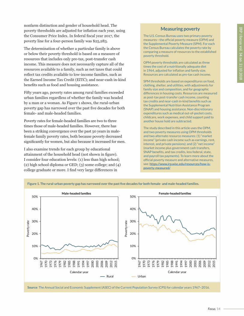
Fifty years ago, poverty rates among rural families exceeded urban families regardless of whether the family was headed by a man or a woman. As Figure 1 shows, the rural-urban poverty gap has narrowed over the past five decades for both female- and male-headed families.
Poverty rates for female-headed families are two to three times those of male-headed families. However, there has been a striking convergence over the past 50 years in male-female family poverty rates, both because poverty decreased significantly for women, but also because it increased for men.
I also examine trends for each group by educational attainment of the household head (not shown in figure). I consider four education levels: (1) less than high school; (2) high school diploma or GED; (3) some college; and (4) college graduate or more. I find very large differences in
Measuring povertyThe U.S. Census Bureau uses two primary poverty measures—the official poverty measure (OPM) and the Supplemental Poverty Measure (SPM). For each the Census Bureau calculates the poverty rate by comparing a measure of resources to the established poverty threshold.
OPM poverty thresholds are calculated as three times the cost of a nutritionally adequate diet in 1964, adjusted for inflation and family size. Resources are calculated as pre-tax cash income.
SPM thresholds are based on expenditures on food, clothing, shelter, and utilities, with adjustments for family size and composition, and for geographic differences in housing costs. Resources are measured as post-tax post-transfer cash income, counting tax credits and near-cash in-kind benefits such as the Supplemental Nutrition Assistance Program (SNAP) and housing assistance. Non-discretionary expenditures such as medical out-of-pocket costs, childcare, work expenses, and child support paid to another house hold are subtracted.
The study described in this article uses the OPM, and two poverty measures using OPM thresholds and two alternate resource measures: (1) “market income” (private cash income such as earnings, rent, interest, and private pensions); and (2) “net income” (market income plus government cash transfers, SNAP benefits, and tax credits, less federal, state, and payroll tax payments). To learn more about the official poverty measure and alternative measures, see: https://www.irp.wisc.edu/resources/how-is-poverty-measured/
Figure 1. The rural-urban poverty gap has narrowed over the past five decades for both female- and male-headed families.
Source: The Annual Social and Economic Supplement (ASEC) of the Current Population Survey (CPS) for calendar years 1967–2016.
0%
10%
20%
30%
40%
50%
1967
1970
1973
1976
1979
1982
1985
1988
1991
1994
1997
2000
2003
2006
2009
2012
2015
Pove
rty
rate
Calendar year
Female-headed families
Rural Urban
0%
10%
20%
30%
40%
50%
1967
1970
1973
1976
1979
1982
1985
1988
1991
1994
1997
2000
2003
2006
2009
2012
2015
Pove
rty
rate
Calendar year
Male-headed families
Focus, 15
IRP | focus vol. 34 no. 2 | 10.2018
poverty status based on educational attainment; in particular, high school dropouts have a poverty rate that is consistently about 15 percentage points higher than that of high school graduates with no college. The trends by education level vary somewhat by gender and urban or rural status. For example, in rural America, poverty among families headed by men with less than a high school diploma doubled, and in urban America nearly tripled, from 1967 to 2016. There have also been substantial increases in poverty among male-headed families with a high school diploma and with some college.
It is clear that the Commission’s goal to “wipe out rural poverty” has not been achieved in the last 50 years. In fact, among the working-age population, progress based on the official poverty measure has either stalled, or for less-skilled men, fallen considerably behind. In the remainder of this article, I examine some possible reasons for these trends, looking first at changes in human capital, family structure, employment and earnings, then at changes in the social safety net.
Rising human capital, retreat from marriage, falling employment, and stagnant earningsFor most Americans, education, marriage, and employment provide the main pathways out of poverty. Accordingly, I look at how each of these factors have changed over time in rural and urban areas.
Trends in educational attainment
Human capital is strongly correlated with income; the evidence suggests that education plays a causal role in earnings—specifically, more education results in more earnings, on average.4 As noted above, the economic status of those with a high school diploma or less has declined over the past 50 years. Therefore, it is important to understand whether the share of the population with a lower level of educational attainment has changed over time, overall, and in urban and rural settings.
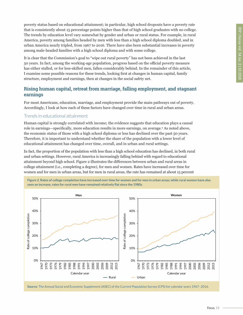
In fact, the proportion of the population with less than a high school education has declined, in both rural and urban settings. However, rural America is increasingly falling behind with regard to educational attainment beyond high school. Figure 2 illustrates the differences between urban and rural areas in college attainment (i.e., completing a degree), for men and women. Rates have increased over time for women and for men in urban areas, but for men in rural areas, the rate has remained at about 15 percent
Figure 2. Rates of college completion have increased over time for women and for men in urban areas; while rural women have also seen an increase, rates for rural men have remained relatively flat since the 1980s.
Source: The Annual Social and Economic Supplement (ASEC) of the Current Population Survey (CPS) for calendar years 1967–2016.
0%
10%
20%
30%
40%
50%
1967
1970
1973
1976
1979
1982
1985
1988
1991
1994
1997
2000
2003
2006
2009
2012
2015
Rate
of c
olle
ge c
ompl
etion
Calendar year
Men
Rural Urban
0%
10%
20%
30%
40%
50%
1967
1970
1973
1976
1979
1982
1985
1988
1991
1994
1997
2000
2003
2006
2009
2012
2015
Rate
of c
olle
ge c
ompl
etion
Calendar year
Women
Focus, 16
IRP | focus vol. 34 no. 2 | 10.2018
since the 1980s. The gap in college attainment between urban and rural men has increased from about 5 percentage points to about 20 percentage points from 1967 to 2016. Among women, those in rural areas have steadily increased their rates of college attainment over the decades, but growth has been much slower than among urban women. Although they started out at similar levels to urban women 50 years ago, rural women now have rates of college completion of about half that of urban women (though rural women now have a greater fraction of the population with some college).
Trends in marriage rates
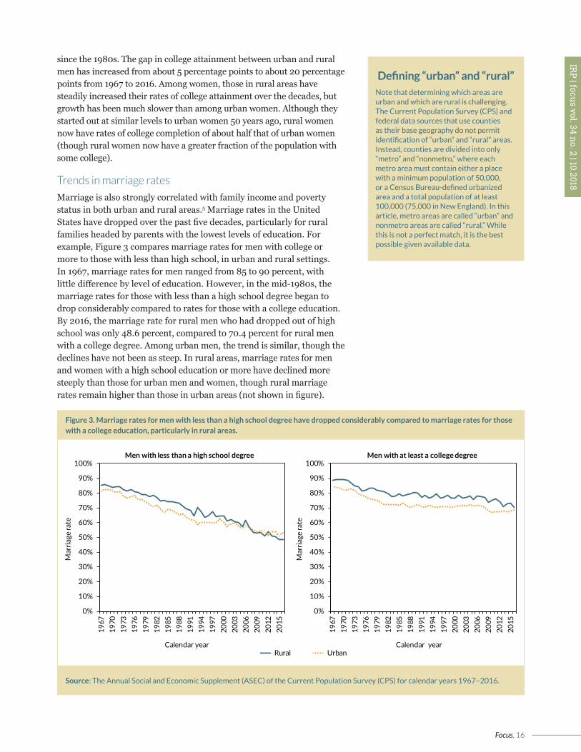
Marriage is also strongly correlated with family income and poverty status in both urban and rural areas.5 Marriage rates in the United States have dropped over the past five decades, particularly for rural families headed by parents with the lowest levels of education. For example, Figure 3 compares marriage rates for men with college or more to those with less than high school, in urban and rural settings. In 1967, marriage rates for men ranged from 85 to 90 percent, with little difference by level of education. However, in the mid-1980s, the marriage rates for those with less than a high school degree began to drop considerably compared to rates for those with a college education. By 2016, the marriage rate for rural men who had dropped out of high school was only 48.6 percent, compared to 70.4 percent for rural men with a college degree. Among urban men, the trend is similar, though the declines have not been as steep. In rural areas, marriage rates for men and women with a high school education or more have declined more steeply than those for urban men and women, though rural marriage rates remain higher than those in urban areas (not shown in figure).
0%
10%
20%
30%
40%
50%
60%
70%
80%
90%
100%
1967
1970
1973
1976
1979
1982
1985
1988
1991
1994
1997
2000
2003
2006
2009
2012
2015
Mar
riage
rate
Calendar year
Men with less than a high school degree
Rural Urban
0%
10%
20%
30%
40%
50%
60%
70%
80%
90%
100%
1967
1970
1973
1976
1979
1982
1985
1988
1991
1994
1997
2000
2003
2006
2009
2012
2015
Mar
riage
rate
Calendar year
Men with at least a college degree
Figure 3. Marriage rates for men with less than a high school degree have dropped considerably compared to marriage rates for those with a college education, particularly in rural areas.
Source: The Annual Social and Economic Supplement (ASEC) of the Current Population Survey (CPS) for calendar years 1967–2016.
Defining “urban” and “rural”Note that determining which areas are urban and which are rural is challenging. The Current Population Survey (CPS) and federal data sources that use counties as their base geography do not permit identification of “urban” and “rural” areas. Instead, counties are divided into only “metro” and “nonmetro,” where each metro area must contain either a place with a minimum population of 50,000, or a Census Bureau-defined urbanized area and a total population of at least 100,000 (75,000 in New England). In this article, metro areas are called “urban” and nonmetro areas are called “rural.” While this is not a perfect match, it is the best possible given available data.
Focus, 17
IRP | focus vol. 34 no. 2 | 10.2018
Trends in employment rates
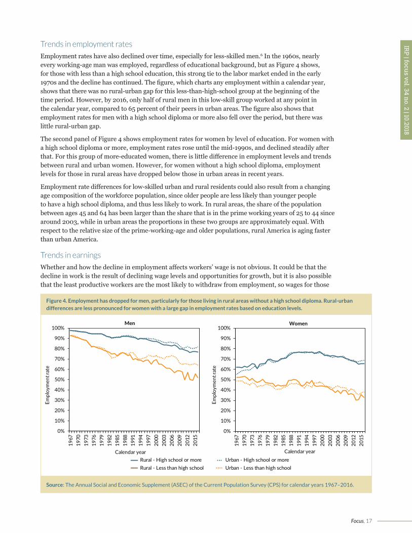
Employment rates have also declined over time, especially for less-skilled men.6 In the 1960s, nearly every working-age man was employed, regardless of educational background, but as Figure 4 shows, for those with less than a high school education, this strong tie to the labor market ended in the early 1970s and the decline has continued. The figure, which charts any employment within a calendar year, shows that there was no rural-urban gap for this less-than-high-school group at the beginning of the time period. However, by 2016, only half of rural men in this low-skill group worked at any point in the calendar year, compared to 65 percent of their peers in urban areas. The figure also shows that employment rates for men with a high school diploma or more also fell over the period, but there was little rural-urban gap.
The second panel of Figure 4 shows employment rates for women by level of education. For women with a high school diploma or more, employment rates rose until the mid-1990s, and declined steadily after that. For this group of more-educated women, there is little difference in employment levels and trends between rural and urban women. However, for women without a high school diploma, employment levels for those in rural areas have dropped below those in urban areas in recent years.
Employment rate differences for low-skilled urban and rural residents could also result from a changing age composition of the workforce population, since older people are less likely than younger people to have a high school diploma, and thus less likely to work. In rural areas, the share of the population between ages 45 and 64 has been larger than the share that is in the prime working years of 25 to 44 since around 2003, while in urban areas the proportions in these two groups are approximately equal. With respect to the relative size of the prime-working-age and older populations, rural America is aging faster than urban America.
Trends in earnings
Whether and how the decline in employment affects workers’ wage is not obvious. It could be that the decline in work is the result of declining wage levels and opportunities for growth, but it is also possible that the least productive workers are the most likely to withdraw from employment, so wages for those
Figure 4. Employment has dropped for men, particularly for those living in rural areas without a high school diploma. Rural-urban differences are less pronounced for women with a large gap in employment rates based on education levels.
Source: The Annual Social and Economic Supplement (ASEC) of the Current Population Survey (CPS) for calendar years 1967–2016.
0%
10%
20%
30%
40%
50%
60%
70%
80%
90%
100%
1967
1970
1973
1976
1979
1982
1985
1988
1991
1994
1997
2000
2003
2006
2009
2012
2015
Empl
oym
ent r
ate
Calendar year
Men
Rural - High school or more Urban - High school or moreRural - Less than high school Urban - Less than high school
0%
10%
20%
30%
40%
50%
60%
70%
80%
90%
100%
1967
1970
1973
1976
1979
1982
1985
1988
1991
1994
1997
2000
2003
2006
2009
2012
2015
Empl
oym
ent r
ate
Calendar year
Women
Focus, 18
IRP | focus vol. 34 no. 2 | 10.2018
remaining in work could increase over time. Based on inflation-adjusted median weekly earnings among workers, it appears that declining wages might be the dominant force driving men’s employment trends, while the exit of less productive workers from the labor market might be a factor among women.
For both rural and urban men with some college or less, real weekly wages peaked in 1973 (just before the first oil crisis), and then fell sharply over the next two decades, especially for men with only high school or less. Wages rose again somewhat with the strong economic expansion of the late 1990s, but it was not sufficient to lift the wages of less-skilled men to 1973 levels. (Figure not shown.)
Prior research on wage inequality has emphasized a shift in employment that favors skilled over unskilled labor, and thus favors those with a college education.7 However, most of this skill premium has gone to men in urban areas; in contrast, real weekly earnings of college-educated men in rural areas have been stuck at about $1,000 for 50 years. Even among college-educated men in urban areas, earnings have not risen considerably in 20 years.
Wages for men in urban areas tend to be higher than those in rural areas, partly due to differences in the cost of living. However, this holds true only for men with college degrees; earnings of lower-skill men do not differ greatly between urban and rural settings.
For women, the trends are more positive than for men; real weekly earnings increased over the period for all groups and regions except the least-skilled. The urban wage premium appears to apply to women with a high school diploma and above (rather than only to those with college degrees, as is the case for men). For women without a high school diploma, as with men, there is no earnings difference between urban and rural settings.
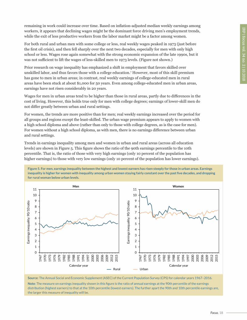
Trends in earnings inequality among men and women in urban and rural areas (across all education levels) are shown in Figure 5. This figure shows the ratio of the 90th earnings percentile to the 10th percentile. That is, the ratio of those with very high earnings (only 10 percent of the population has higher earnings) to those with very low earnings (only 10 percent of the population has lower earnings).
Figure 5. For men, earnings inequality between the highest and lowest earners has risen steeply for those in urban areas. Earnings inequality is higher for women with inequality among urban women staying fairly constant over the past five decades, and dropping for rural woman below urban levels.
Source: The Annual Social and Economic Supplement (ASEC) of the Current Population Survey (CPS) for calendar years 1967–2016.
Note: The measure on earnings inequality shown in this figure is the ratio of annual earnings at the 90th percentile of the earnings distribution (highest earners) to that at the 10th percentile (lowest earners). The further apart the 90th and 10th percentile earnings are, the larger this measure of inequality will be.
0
1
2
3
4
5
6
7
8
9
10
11
1967
1970
1973
1976
1979
1982
1985
1988
1991
1994
1997
2000
2003
2006
2009
2012
2015
Earn
ings
ineq
ualit
y: 9
0/10
ratio
Calendar year
Men
Rural Urban
0
1
2
3
4
5
6
7
8
9
10
11
1967
1970
1973
1976
1979
1982
1985
1988
1991
1994
1997
2000
2003
2006
2009
2012
2015
Earn
ings
ineq
ualit
y: 9
0/10
ratio
Calendar year
Women
Focus, 19
IRP | focus vol. 34 no. 2 | 10.2018
This figure shows that the much-discussed rise in earnings inequality is an issue primarily facing men in urban settings; at the beginning of the time period, inequality was higher in rural areas. Over the past 50 years, the high-to-low earnings ratio among urban men doubled, while for rural men it rose sharply in the early 1980s, but then dropped again in the late 1990s. While women in both urban and rural settings earn lower wages than men, the level of inequality between the highest earners and the lowest earners has generally been more pronounced for women than it is for men. For urban women, this measure of inequality is largely unchanged over the time period. Rural women had much higher levels of inequality than urban women at the beginning of the period, but that dropped particularly in the 1970s, so that rural women now have lower levels of earnings inequality.
The rising importance of social assistance in rural AmericaThe U.S. social safety net is large, exceeding over $2 trillion in annual spending, and on a per capita basis has more than quadrupled since 1970.8 The programs that compose the safety net are typically grouped into two broad categories, social insurance programs and means-tested transfers (see text box).
Although none of these programs specifically target urban or rural residents, we might expect the effects of the safety net to vary in different areas, given the differences in education, work, wages, and population aging discussed above. In order to evaluate rural-urban differences, I look first at trends in the share of income transfers as a fraction of personal income.
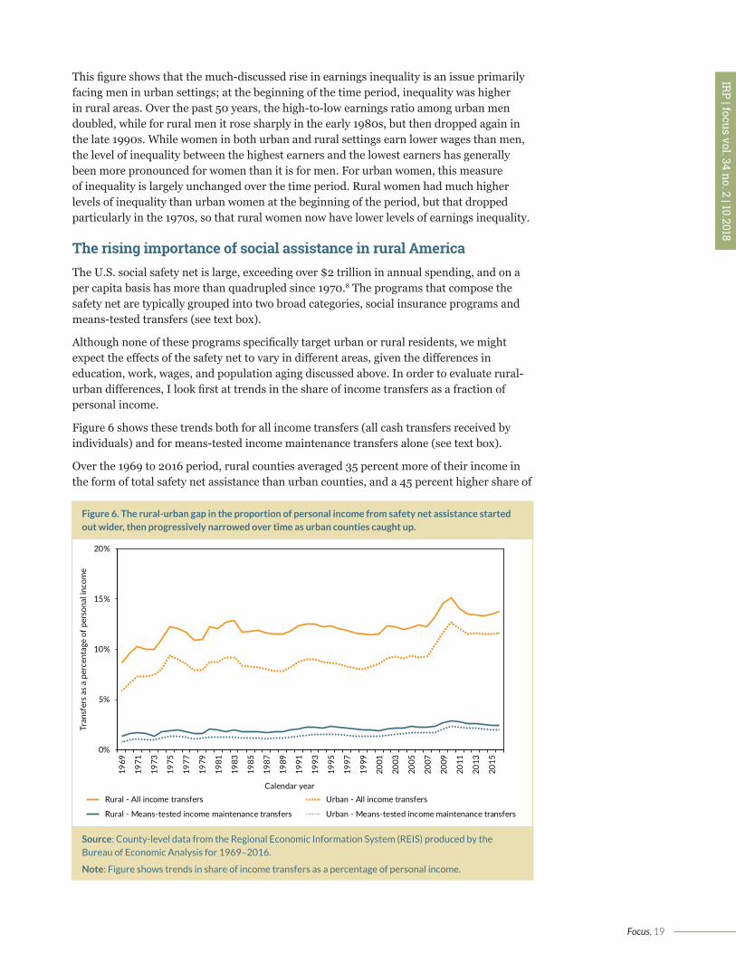
Figure 6 shows these trends both for all income transfers (all cash transfers received by individuals) and for means-tested income maintenance transfers alone (see text box).
Over the 1969 to 2016 period, rural counties averaged 35 percent more of their income in the form of total safety net assistance than urban counties, and a 45 percent higher share of
Figure 6. The rural-urban gap in the proportion of personal income from safety net assistance started out wider, then progressively narrowed over time as urban counties caught up.
Source: County-level data from the Regional Economic Information System (REIS) produced by the Bureau of Economic Analysis for 1969–2016.
Note: Figure shows trends in share of income transfers as a percentage of personal income.
0%
5%
10%
15%
20%
1969
1971
1973
1975
1977
1979
1981
1983
1985
1987
1989
1991
1993
1995
1997
1999
2001
2003
2005
2007
2009
2011
2013
2015
Tran
sfer
s as
a p
erce
ntag
e of
per
sona
l inc
ome
Calendar yearRural - All income transfers Urban - All income transfers
Rural - Means-tested income maintenance transfers Urban - Means-tested income maintenance transfers
Focus, 20
IRP | focus vol. 34 no. 2 | 10.2018
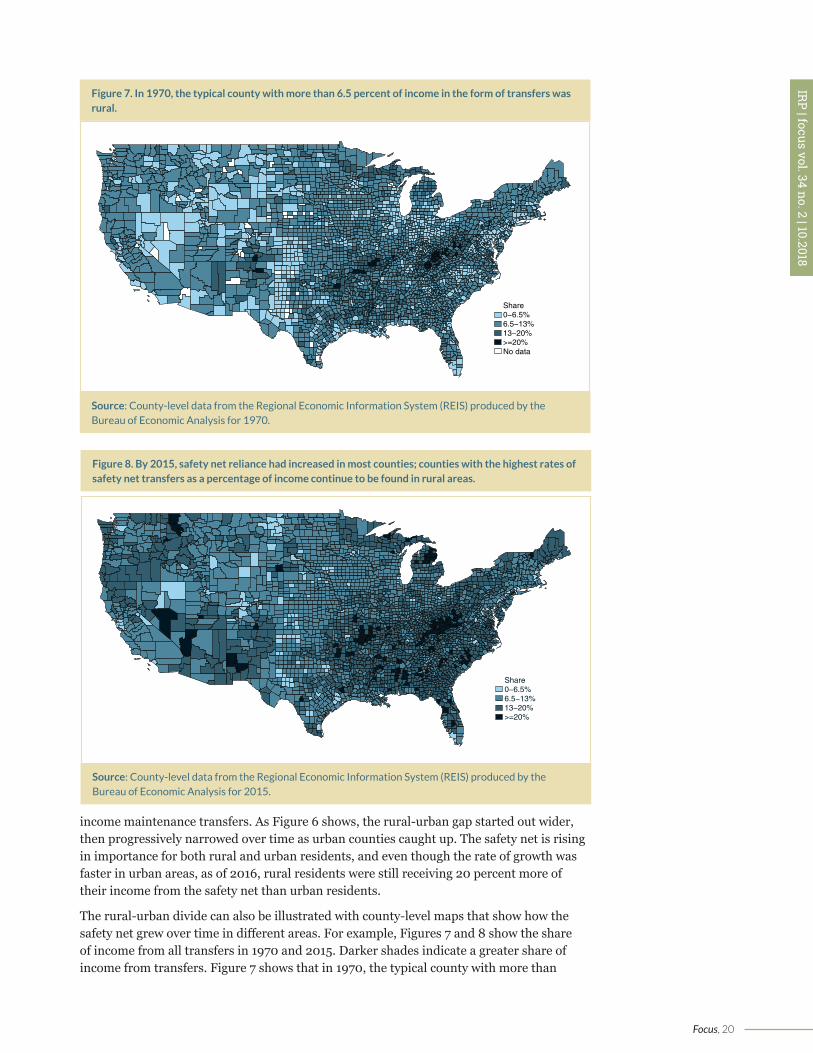
Figure 7. In 1970, the typical county with more than 6.5 percent of income in the form of transfers was rural.
Source: County-level data from the Regional Economic Information System (REIS) produced by the Bureau of Economic Analysis for 1970.
Figure 8. By 2015, safety net reliance had increased in most counties; counties with the highest rates of safety net transfers as a percentage of income continue to be found in rural areas.
Source: County-level data from the Regional Economic Information System (REIS) produced by the Bureau of Economic Analysis for 2015.
Share0−6.5%6.5−13%13−20%>=20%No data
Share0−6.5%6.5−13%13−20%>=20%
income maintenance transfers. As Figure 6 shows, the rural-urban gap started out wider, then progressively narrowed over time as urban counties caught up. The safety net is rising in importance for both rural and urban residents, and even though the rate of growth was faster in urban areas, as of 2016, rural residents were still receiving 20 percent more of their income from the safety net than urban residents.
The rural-urban divide can also be illustrated with county-level maps that show how the safety net grew over time in different areas. For example, Figures 7 and 8 show the share of income from all transfers in 1970 and 2015. Darker shades indicate a greater share of income from transfers. Figure 7 shows that in 1970, the typical county with more than
Focus, 21
IRP | focus vol. 34 no. 2 | 10.2018
6.5 percent of income in the form of transfers was rural, with areas such as central Appalachia, the Mississippi Delta region, and some Native American counties in the mountain West already having over 20 percent of income from transfers. The areas historically meet the U.S. Department of Agriculture (USDA) definition of “persistently poor.”9
Figure 8 shows that over the next 45 years, safety net reliance increased in most counties except some particularly economically vibrant major urban centers and select rural counties. The counties with very high rates, in excess of 20 percent of income, continue to be found in rural areas, and in particular those areas most associated with persistent poverty.
Progress against (unofficial) povertyWhile increased reliance on the safety net is concerning, without the expansion of social assistance programs, material hardship in rural America would be much worse today than it was 50 years ago. In many respects, the safety net has stepped in to fill the gap where the private sector economy has failed. A comparison of trends in the percentage of families in poverty measured using private income alone (earnings, rent, interest, dividends, private pensions) and official poverty measure thresholds, to poverty measured using an after-tax and transfer measure of net income, including net payroll taxes, shows that for most groups and years, the safety net, broadly defined, lifts more families in rural areas out of market poverty (that is, poverty measured by the official poverty measure) than similarly situated families in urban areas.
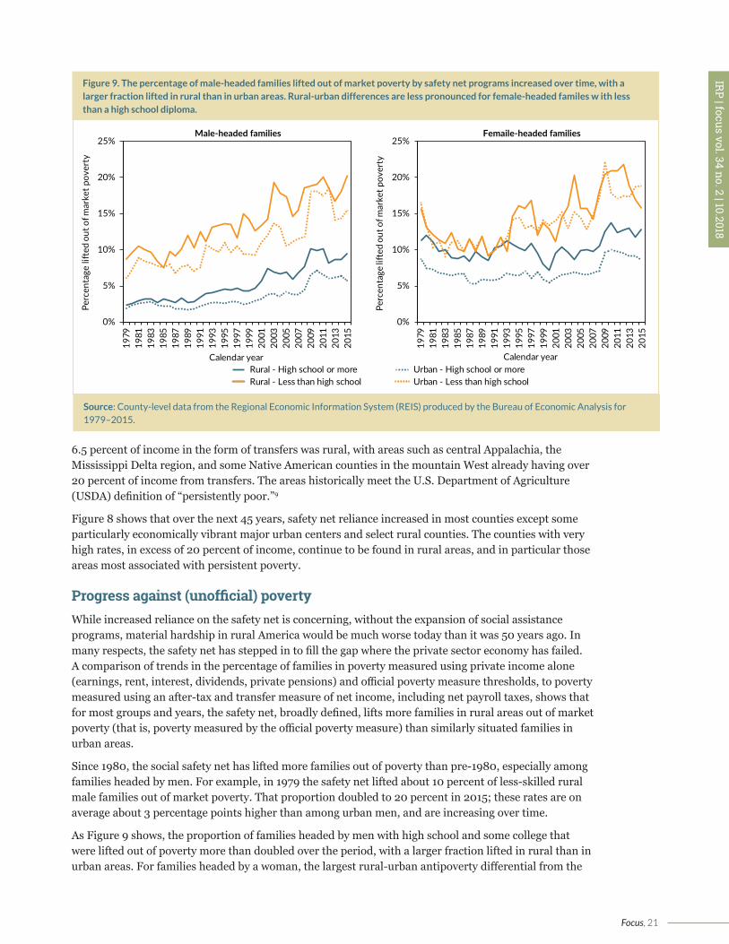
Since 1980, the social safety net has lifted more families out of poverty than pre-1980, especially among families headed by men. For example, in 1979 the safety net lifted about 10 percent of less-skilled rural male families out of market poverty. That proportion doubled to 20 percent in 2015; these rates are on average about 3 percentage points higher than among urban men, and are increasing over time.
As Figure 9 shows, the proportion of families headed by men with high school and some college that were lifted out of poverty more than doubled over the period, with a larger fraction lifted in rural than in urban areas. For families headed by a woman, the largest rural-urban antipoverty differential from the
Figure 9. The percentage of male-headed families lifted out of market poverty by safety net programs increased over time, with a larger fraction lifted in rural than in urban areas. Rural-urban differences are less pronounced for female-headed familes w ith less than a high school diploma.
Source: County-level data from the Regional Economic Information System (REIS) produced by the Bureau of Economic Analysis for 1979–2015.
0%
5%
10%
15%
20%
25%19
7919
8119
8319
8519
8719
8919
9119
9319
9519
9719
9920
0120
0320
0520
0720
0920
1120
1320
15
Perc
enta
ge lift
ed o
ut o
f mar
ket p
over
ty
Calendar year
Male-headed families
Rural - High school or more Urban - High school or moreRural - Less than high school Urban - Less than high school
0%
5%
10%
15%
20%
25%
1979
1981
1983
1985
1987
1989
1991
1993
1995
1997
1999
2001
2003
2005
2007
2009
2011
2013
2015
Perc
enta
ge lift
ed o
ut o
f mar
ket p
over
ty
Calendar year
Femaile-headed families
Focus, 22
IRP | focus vol. 34 no. 2 | 10.2018
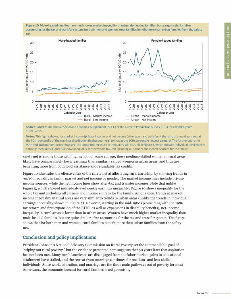
Figure 10. Male-headed families have much lower market inequality than female-headed families, but are quite similar after accounting for the tax and transfer system; for both men and women, rural families benefit more than urban families from the safety net.
Source: Source: The Annual Social and Economic Supplement (ASEC) of the Current Population Survey (CPS) for calendar years 1979–2015.
Notes: This figure shows, for market income (private income) and net income (after taxes and transfers), the ratio of annual earnings at the 90th percentile of the earnings distribution (highest earners) to that at the 10th percentile (lowest earners). The further apart the 90th and 10th percentile earnings are, the larger this measure of inequality will be. Unlike Figure 5, which showed individual-level weekly earnings inequality, Figure 10 shows inequality for the whole tax unit including all earners and income sources for the family.
safety net is among those with high school or some college; these medium-skilled women in rural areas likely have comparatively lower earnings than similarly skilled women in urban areas, and thus are benefiting more from both food assistance and refundable tax credits.
Figure 10 illustrates the effectiveness of the safety net at alleviating rural hardship, by showing trends in 90/10 inequality in family market and net income by gender. The market income lines include private income sources, while the net income lines show after-tax and transfer incomes. Note that unlike Figure 5, which showed individual-level weekly earnings inequality, Figure 10 shows inequality for the whole tax unit including all earners and income sources for the family. Among men, trends in market income inequality in rural areas are very similar to trends in urban areas (unlike the trends in individual earnings inequality shown in Figure 5). However, starting in the mid-1980s (coinciding with the 1986 tax reform and first expansion of the EITC, as well as expansions in disability benefits), net-income inequality in rural areas is lower than in urban areas. Women have much higher market inequality than male-headed families, but are quite similar after accounting for the tax and transfer system. The figure shows that for both men and women, rural families benefit more than urban families from the safety net.
Conclusion and policy implicationsPresident Johnson’s National Advisory Commission on Rural Poverty set the commendable goal of “wiping out rural poverty,” but the evidence presented here suggests that 50 years later that aspiration has not been met. Many rural Americans are disengaged from the labor market, gains in educational attainment have stalled, and the retreat from marriage continues for medium- and less-skilled individuals. Since work, education, and marriage are the three main pathways out of poverty for most Americans, the economic forecast for rural families is not promising.
0
5
10
15
20
25
30
1979
1981
1983
1985
1987
1989
1991
1993
1995
1997
1999
2001
2003
2005
2007
2009
2011
2013
2015
Mar
ket i
nequ
ality
: 90/
10 ratio
Calendar year
Male-headed families
Rural - Market income Urban - Market incomeRural - Net income Urban - Net income
0
5
10
15
20
25
30
1979
1981
1983
1985
1987
1989
1991
1993
1995
1997
1999
2001
2003
2005
2007
2009
2011
2013
2015
Mar
ket i
nequ
ality
: 90/
10 ratio
Calendar year
Female-headed families
Focus, 23
IRP | focus vol. 34 no. 2 | 10.2018
The evidence presented here adds to the literature showing that in the absence of the expanding safety net, economic hardship would have been much worse for rural America. While concerns that the structure of the safety net creates disincentives to work and marriage may be justified, evidence consistently shows that these disincentive effects are small in magnitude, and that reliance on assistance programs is a consequence, and not a cause, of the poverty witnessed in recent decades.10 The Commission expressed frustration that the poverty-fighting efforts of the time were largely targeted to urban areas. However, in the intervening decades the boundaries have been blurred between urban and rural places when it comes to major tax and transfer programs, and in fact rural people are more likely to be lifted out of market-income poverty and face lower after-tax and transfer inequality compared to their urban counterparts.
Going forward, however, the drop in employment among the rural poor could eventually lead to less assistance from the safety net, as policymakers continue to remake safety net programs to favor those who are working over those who are not. The EITC expansions of the early 1990s, combined with the 1996 welfare reform, were the first major steps in this direction, requiring work to qualify for the EITC, and requiring most adult recipients on Temporary Assistance for Needy Families (TANF) to engage in work activities and be subject to time limits on the receipt of aid. The 1996 legislation also expanded work requirements for food stamps to able-bodied adults without dependents between the ages of 18 and 49. Currently, there are efforts in various state legislatures and in Congress to increase work requirements, and to expand these requirements to other safety net programs such as Medicaid.
These work requirements are based on the premise that work (or now, full-time work) is readily available for those who are willing and able. However, the demand for labor is lacking in many rural communities, especially those most distant from urban centers. This suggests that an economic policy that facilitates access to work, including direct place-based employment programs, will be necessary if the Commission’s dream of full employment and eradicating rural poverty is to be realized.11n
Safety net programsThe safety net comprises two categories of assistance, social insurance programs and means-tested transfers.
Social insurance programs are tied to employment, military service, or old age, and include:
• Social Security Retirement and Survivors Benefits
• Disability Insurance
• Medicare
• Unemployment Insurance
• Veterans Benefits
• Workers Compensation
Means-tested transfers are conditioned on low income, and often low assets, but typically not employment or age, and include:
• Medicaid
• Supplemental Security Income (SSI)*
• Temporary Assistance for Needy Families (TANF)— formerly Aid to Families with Dependent Children (AFDC)*
• General assistance*
• Housing assistance
• Supplemental Nutrition Assistance Program (SNAP)—formerly Food Stamps*
• National School Breakfast and Lunch Programs
• Special Supplemental Nutrition Assistance Program for Women, Infants, and Children (WIC).
Two important means-tested programs that are directly tied to employment are:
• Earned Income Tax Credit (EITC) *
• Additional Child Tax Credit (ACTC)
*Programs counted as means-tested income maintenance transfers in this article.
1 E. Breathitt, The People Left Behind: A Report by the President’s National Advisory Commission on Rural Poverty, Washington, D.C., 1967.2 This article is based on an invited paper for the 2018 Rural Poverty Research Conference, “Rural Poverty: Fifty Years After The People Left Behind.” The paper, J. P. Ziliak, “Economic Change and the Social Safety Net: Are Rural Americans Still Behind?” may be accessed at http://www.rupri.org/wp-content/uploads/Economic-Change-and-the-Social-Safety-Net-2.pdf.3 M. Orshansky, “Children of the Poor,” Social Security Bulletin 26, No. 7 (1963): 3–13.4 D. Card, “The Causal Effect of Education on Earnings,” in Handbook of Labor Economics, Vol 3A, eds. O. Ashenfelter and D. Card (Amsterdam: North Holland, 1999 Ch. 30).
Focus, 24
IRP | focus vol. 34 no. 2 | 10.2018
Type of analysis: Descriptive
Data source: The Annual Social and
Economic Supplement (ASEC) of the
Current Population Survey (CPS) for
calendar years 1967–2016, and county-
level data from the Regional Economic
Information System (REIS) produced
by the Bureau of Economic Analysis for
1969–2016. The ASEC is the official source
of government statistics on poverty and
inequality, while the REIS is the primary
source for tracking the geographic
distribution of income and employment
over time.
Type of data: Survey
Unit of analysis: Individual (ASEC) and
county (REIS)
Sample definition: The sample is restricted
to the civilian population between the ages
of 25 and 64, in order to include those most
likely to have completed formal schooling
and be of working age.
Poverty definition used: Official poverty
measure
Time frame: Calendar years 1967 through
2016
Limitations: Metro and nonmetro
definitions do not line up perfectly with
urban and rural. This analysis is descriptive,
not causal.
Sou
rces
& M
eth
od
s5M. Cancian and D. Reed, “Changes in Family Structure: Implications for Poverty and Related Policy,” in Understanding Poverty, eds. S. Danziger and R. Haveman (Cambridge, MA: Harvard University Press, 2001); D. Lichter and L. Cimbaluk, “Family Change and Poverty in Appalachia,” in Appalachian Legacy: Economic Opportunity after the War on Poverty, ed. J. Ziliak (Washington, D.C.: Brookings Institution, 2012).6N. Eberstadt, Men Without Work: America’s Invisible Crisis (West Conshohocken, PA: Templeton Press, 2016).7 See, for example, D. Autor, L. Katz, and M. Kearney, “Trends in U.S. Wage Inequality: Revising the Revisionists,” Review of Economics and Statistics 90 (2008): 300–323.8R. Moffitt, “The Great Recession and the Social Safety Net,” The ANNALS of the American Academy of Political and Social Science 650 (2013): 143–166.9 Persistent poverty counties are those where 20 percent of more of county residents were poor over the past 30 years according to census data.10See, for example, M. Bitler and H. Hoynes, “The More Things Change, the More They Stay the Same? The Safety Net and Poverty in the Great Recession,” Journal of Labor Economics 34 (2016): S403–S444.11B. Austin, E. Glaeser, and L. Summers, “Saving the Heartland: Place-Based Policies in 21st Century America,” Brookings Papers on Economic Activity, March 8, 2018.
IRPfocus
Focus has a new look!Thanks to Riley Tsang and Dawn Duren
for their work on the redesign.
Institute for Research on PovertyUniversity of Wisconsin–Madison3412 William H. Sewell Social Science Building1180 Observatory DriveMadison, WI 53706