Vol. 13, No. 1

TNT · January 2017 · 1

FOCUS

IntroductionPositive material identification (PMI) is an essential component of construction, maintenance, and safety in chemical, petroleum, and power generation plants. Failure to use the proper alloy in each application can result in production loss but, more importantly, it is a threat to the health, safety, and well-being of the public. In the United States, the Occupational Safety and Health Administration, the Department of Transportation Pipeline and Hazardous Materials Safety Administration, the American Petroleum Institute, the National Transportation Safety Board, the Bureau of Safety and Environmental Enforcement, and NACE International have all recommended the implementation of PMI programs in their respective spheres of influence (API, 2010; API, 2013; OSHA, 1998; PHMSA, 2009; PHMSA, 2015).

Handheld X-ray fluorescence (XRF) is a highly effective technique for PMI. The combination of fundamental science, modern electronics, and digital computing result in a technique that is simple, accurate, and precise. The nondestructive testing (NDT) technician is able to obtain definitive elemental analysis and alloy grade matching with little to no specimen preparation. Typically, this can all be accomplished in less than 30 seconds, with many commercial alloys being identified with only 2 to 3 seconds of test time. This ease of use enables fast and extensive testing, even on in-service samples.

Given the critical nature of PMI, NDT technicians often wonder about the accuracy and precision of XRF instruments. How confident can they be in their measurements? This article clarifies the meaning and implications of accuracy, precision, and confidence level as they apply to XRF for PMI.

Accuracy, Precision, and Confidence in X-ray Fluorescence for Positive Material Identificationby Michael W. Hull

From NDT Technician Newsletter, Vol. 16, No. 1, pp: 1-6.Copyright © 2017 The American Society for Nondestructive Testing, Inc.

17Jan TNT GoogleScholar.indd 1 12/29/16 2:44 PM

2 · Vol. 16, No. 1

FOCUS | Positive Material Identification

l Accuracy asks, “How close are the measurements to the true value?”

l Precision asks, “How close are the measurements to each other?”

l Confidence level asks, “How sure are you that the measurement is correct?”XRF measurements involve several

sequential steps that appear seamless and instantaneous to the NDT technician, but are separate on the level of physics and electronics: 1. X-rays are emitted from the instrument

and the sample is irradiated. (In handheld XRF, X-rays can come from one of two sources: miniaturized X-ray tubes or radioactive sources. In North America, the majority of XRF analyzers employ miniaturized X-ray tubes. These operate by passing an electric current across the cathode, accelerating electrons toward the anode, which then emits the X-rays. Historically, XRF analyzers, and some units still on the market, employ radioactive isotope samples as their X-ray sources. These generate X-ray by a radioactive nuclear decay process.)

2. The atoms in the sample absorb the X-rays and are excited to a higher energy state.

3. The atoms in the sample re-emit their own characteristic X-rays, reflecting the elemental composition of the sample.

4. The characteristic X-rays are measured by a digital detector in the instrument.

5. The signal from the digital detector is analyzed and interpreted using computer software and analysis.

6. The NDT technician is provided a grade match and elemental composition. The resulting measurement enables the technician to assess his or her confidence level in the analyzer’s accuracy and precision.

Accuracy in X-ray Fluorescence MeasurementsXRF is very accurate, measuring most of the common metals in alloys (for example, iron, nickel, copper, and so on) to less than 0.01%. Although most of the elements on the periodic table can be detected and

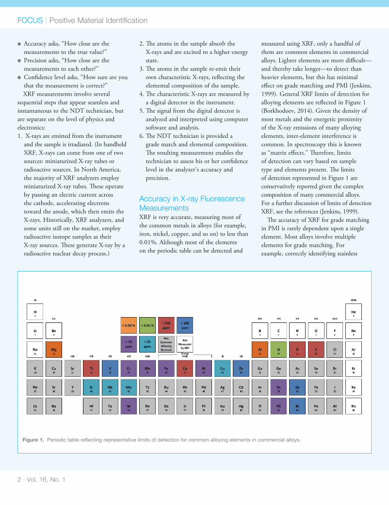
measured using XRF, only a handful of them are common elements in commercial alloys. Lighter elements are more difficult—and thereby take longer—to detect than heavier elements, but this has minimal effect on grade matching and PMI (Jenkins, 1999). General XRF limits of detection for alloying elements are reflected in Figure 1 (Borkhodoev, 2014). Given the density of most metals and the energetic proximity of the X-ray emissions of many alloying elements, inter-element interference is common. In spectroscopy this is known as “matrix effects.” Therefore, limits of detection can vary based on sample type and elements present. The limits of detection represented in Figure 1 are conservatively reported given the complex composition of many commercial alloys. For a further discussion of limits of detection XRF, see the references (Jenkins, 1999).

The accuracy of XRF for grade matching in PMI is rarely dependent upon a single element. Most alloys involve multiple elements for grade matching. For example, correctly identifying stainless

Figure 1. Periodic table reflecting representative limits of detection for common alloying elements in commercial alloys.

17Jan TNT GoogleScholar.indd 2 12/29/16 2:44 PM

steel 321 (Figure 2) depends on the alloy requirements for iron, chromium, nickel, and titanium, along with specific allowances for manganese, copper, and molybdenum. This grade identification does not depend solely on the accuracy of a single element (for example, chromium) but upon measuring multiple elements (for example, iron, nickel, and titanium along with the chromium). This improves the accuracy of the identification. It is analogous to having multi-point identification in forensics (that is, sex, height, weight, hair color, fingerprints, and blood type).

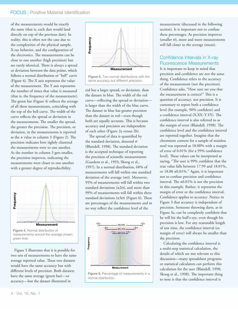
It is important to keep in mind that accuracy and precision are two different and independent qualities of a measurement (Guare, 1991; Treptow, 1998). Both are important, but they are not the same thing. Accuracy reflects how close the measurement is to the sample’s true value, while precision determines how close repeated measurements are to each other. This distinction can be illustrated using a target (Figure 3). Accuracy in this

illustration asks, “How close are the hits to the bull’s-eye?” Hitting the bull’s-eye is equivalent to correctly measuring the true value. A measurement is deemed accurate if it is in agreement with the true value (Jenkins, 1999). In other words, “Is the measurement correct?”

Precision in X-ray Fluorescence MeasurementsPrecision in this illustration asks “How close are the hits to one another?” Note in Figure 3 that it is possible to have high accuracy (close to the bull’s-eye) with low precision (Figure 3a). It is also possible to have high precision (close to each other) with low accuracy (Figure 3b). A measurement is deemed precise if it is in agreement with other repetitions of that same measurement—independent of whether they reflect the true value. In other words, “Is the measurement reproducible?” A properly designed and calibrated XRF analyzer is able to provide a measurement that is both accurate and precise (Figure 3c).

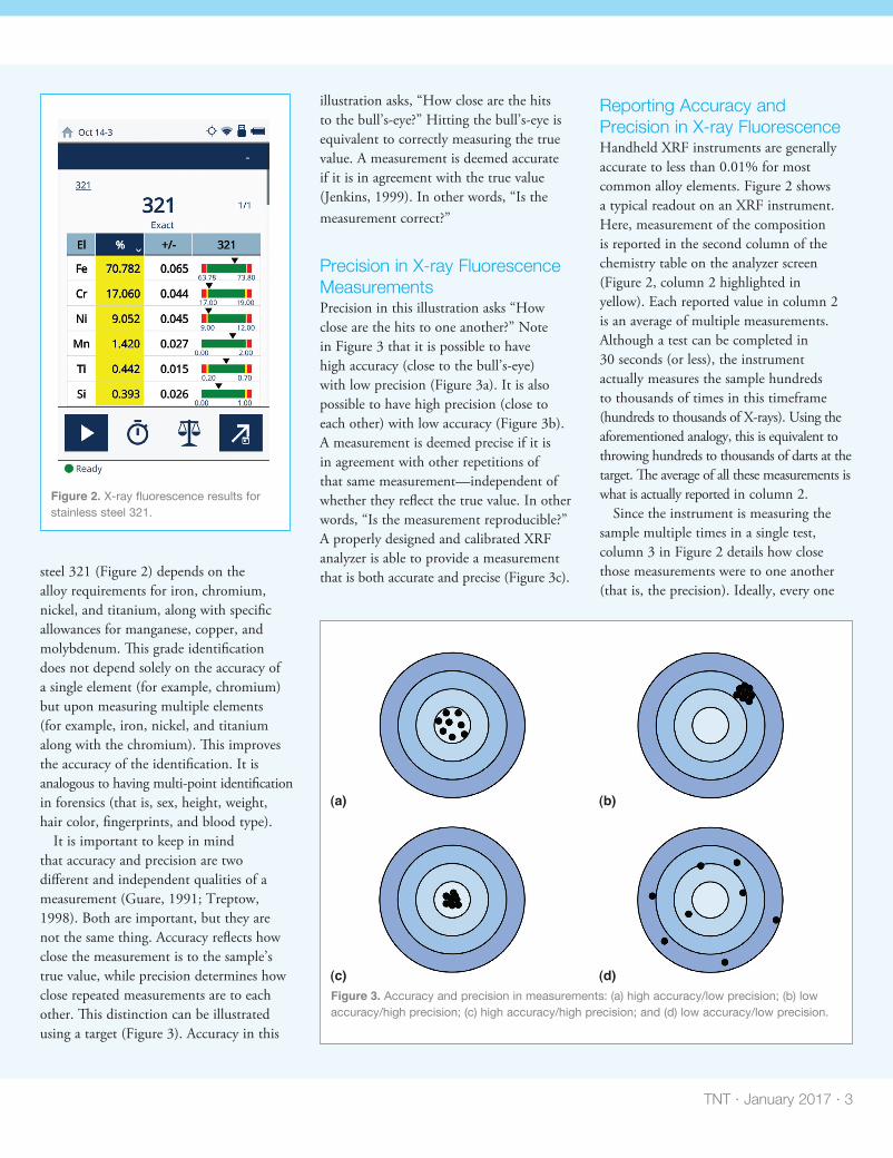
Reporting Accuracy and Precision in X-ray FluorescenceHandheld XRF instruments are generally accurate to less than 0.01% for most common alloy elements. Figure 2 shows a typical readout on an XRF instrument. Here, measurement of the composition is reported in the second column of the chemistry table on the analyzer screen (Figure 2, column 2 highlighted in yellow). Each reported value in column 2 is an average of multiple measurements. Although a test can be completed in 30 seconds (or less), the instrument actually measures the sample hundreds to thousands of times in this timeframe (hundreds to thousands of X-rays). Using the aforementioned analogy, this is equivalent to throwing hundreds to thousands of darts at the target. The average of all these measurements is what is actually reported in column 2.

Since the instrument is measuring the sample multiple times in a single test, column 3 in Figure 2 details how close those measurements were to one another (that is, the precision). Ideally, every one

TNT · January 2017 · 3

Figure 2. X-ray fluorescence results for stainless steel 321.

Figure 3. Accuracy and precision in measurements: (a) high accuracy/low precision; (b) low accuracy/high precision; (c) high accuracy/high precision; and (d) low accuracy/low precision.

(a)

(c)

(b)

(d)

17Jan TNT GoogleScholar.indd 3 12/29/16 2:44 PM

4 · Vol. 16, No. 1

of the measurements would be exactly the same (that is, each dart would land directly on top of the previous dart). In reality, this is often not the case due to the complexities of the physical sample, X-ray behavior, and the confi guration of the electronics. Th e measurements can be close to one another (high precision) but are rarely identical. Th ere is always a spread or deviation between the data points, which follows a normal distribution or “bell” curve (Figure 4). Th e X axis represents the value of the measurement. Th e Y axis represents the number of times that value is measured (that is, the frequency of the measurement). Th e green bar (Figure 4) refl ects the average of all these measurements, coinciding with the top of the bell curve. Th e width of the curve refl ects the spread or deviation in the measurements. Th e smaller the spread, the greater the precision. Th e precision, or deviation, in the measurements is reported as the ± value in column 3 (Figure 2). Th e precision indicates how tightly clustered the measurements were to one another. As the number in column 3 gets smaller, the precision improves, indicating the measurements were closer to one another with a greater degree of reproducibility.

Figure 5 illustrates that it is possible for two sets of measurements to have the same average reported value. Th ese two datasets would have the same accuracy but with diff erent levels of precision. Both datasets have the same average (green bar)—or accuracy—but the dataset illustrated in

red has a larger spread, or deviation, than the dataset in blue. Th e width of the red curve—refl ecting the spread or deviation—is larger than the width of the blue curve. Th e dataset in blue has greater precision than the dataset in red—even though both are equally accurate. Th is is because accuracy and precision are independent of each other (Figure 2a versus 2b).

Th e spread of data is quantifi ed by the standard deviation, denoted s (Blaisdell, 1998). Th e standard deviation is the accepted technique of reporting the precision of scientifi c measurements (Guedens et al., 1993; Skoog et al., 1997). In a normal distribution, 68% of measurements will fall within one standard deviation of the average (±s). Moreover, 95% of measurements will fall within two standard deviations (±2s), and more than 99% of measurements will fall within three standard deviations (±3s) (Figure 6). Th ese are percentages of the measurements and in no way refl ect the confi dence level of the

measurement (discussed in the following section). It is important not to confuse these percentages. As precision improves (smaller s), more and more measurements will fall closer to the average (mean).

Confi dence Intervals in X-ray Fluorescence MeasurementsIt is important to keep in mind that precision and confi dence are not the same thing. Confi dence refers to the accuracy of the measurement (not the precision). Confi dence asks, “How sure are you that the measurement is correct?” Th is is a question of accuracy, not precision. It is customary to report both a confi dence level (for example, 90% confi dent) and a confi dence interval (X.XX‒Y.YY). Th e confi dence interval is also referred to as the margin of error (Blaisdell, 1998). Th e confi dence level and the confi dence interval are reported together. Imagine that the chromium content for a sample of stainless steel was reported as 18.00% with a margin of error of 0.01% (for a 99% confi dence level). Th ese values can be interpreted as saying, “Th e user is 99% confi dent that the true value falls between 17.99 and 18.01%, or 18.00 ±0.01%.” Again, it is important not to confuse precision and confi dence interval. Th e ±0.01% is not the precision in this example. Rather, it represents the margin of error or the confi dence interval. Confi dence applies to accuracy. Notice in Figure 3 that accuracy is independent of precision. Someone throwing darts, as in Figure 3a, can be completely confi dent that he will hit the bull’s-eye, even though his precision is low. For any reasonable length of test time, the confi dence interval (or margin of error) will always be smaller than the precision.

Calculating the confi dence interval is a multi-step statistical calculation, the details of which are not relevant to this discussion—many spreadsheet programs or statistical calculators can perform this calculation for the user (Blaisdell, 1998; Skoog et al., 1998). Th e important thing to note is that the confi dence interval is

FOCUS | Positive Material Identifi cation

Figure 4. Normal distribution of measurements around the average (mean; green line).

Figure 5. Two normal distributions with the same accuracy but different precision.

Figure 6. Percentage of measurements in a normal distribution.

17Jan TNT GoogleScholar.indd 4 12/29/16 2:44 PM

inversely proportional to the number of measurements (usually a function of test time). The longer the test time (seconds), the smaller the confidence interval—which is a good thing. It is also worth noting that the confidence interval is directly proportional to the confidence level. In other words, for the same measurement (for example, 18.00%), a 90% confidence level will have a confidence interval of ±0.047, a 95% confidence level will have a confidence interval of ±0.055, and a 99% confidence level will have a confidence interval of ±0.072. In order to be “more sure,” the range must be opened up more. This interval can be thought of like a dragnet—the bigger the net, the greater the chances of “catching” the right thing.

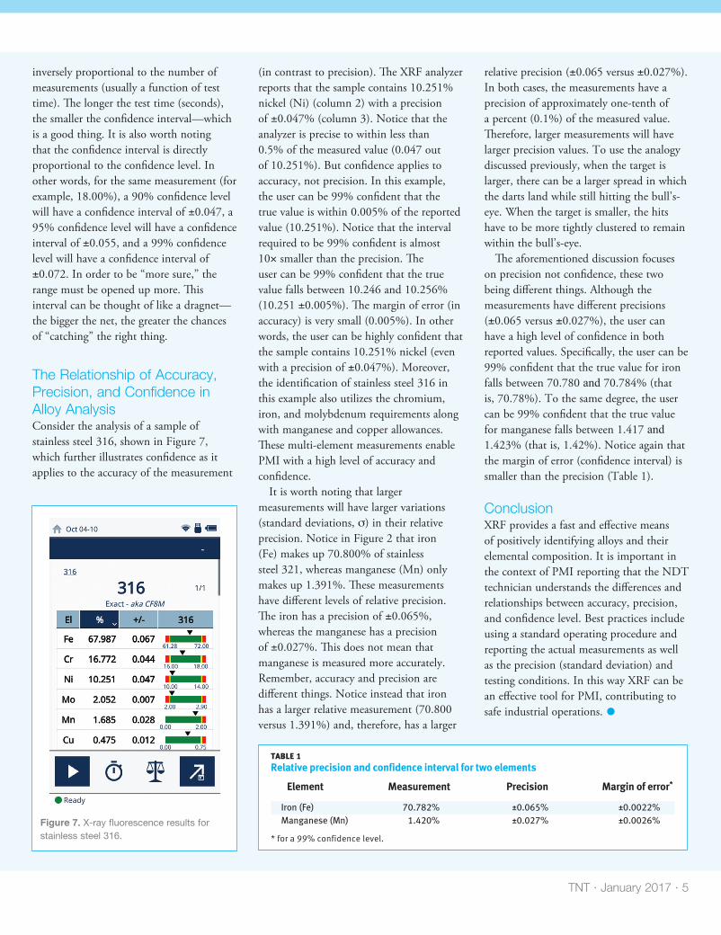
The Relationship of Accuracy, Precision, and Confidence in Alloy AnalysisConsider the analysis of a sample of stainless steel 316, shown in Figure 7, which further illustrates confidence as it applies to the accuracy of the measurement

(in contrast to precision). The XRF analyzer reports that the sample contains 10.251% nickel (Ni) (column 2) with a precision of ±0.047% (column 3). Notice that the analyzer is precise to within less than 0.5% of the measured value (0.047 out of 10.251%). But confidence applies to accuracy, not precision. In this example, the user can be 99% confident that the true value is within 0.005% of the reported value (10.251%). Notice that the interval required to be 99% confident is almost 10× smaller than the precision. The user can be 99% confident that the true value falls between 10.246 and 10.256% (10.251 ±0.005%). The margin of error (in accuracy) is very small (0.005%). In other words, the user can be highly confident that the sample contains 10.251% nickel (even with a precision of ±0.047%). Moreover, the identification of stainless steel 316 in this example also utilizes the chromium, iron, and molybdenum requirements along with manganese and copper allowances. These multi-element measurements enable PMI with a high level of accuracy and confidence.

It is worth noting that larger measurements will have larger variations (standard deviations, s) in their relative precision. Notice in Figure 2 that iron (Fe) makes up 70.800% of stainless steel 321, whereas manganese (Mn) only makes up 1.391%. These measurements have different levels of relative precision. The iron has a precision of ±0.065%, whereas the manganese has a precision of ±0.027%. This does not mean that manganese is measured more accurately. Remember, accuracy and precision are different things. Notice instead that iron has a larger relative measurement (70.800 versus 1.391%) and, therefore, has a larger

relative precision (±0.065 versus ±0.027%). In both cases, the measurements have a precision of approximately one-tenth of a percent (0.1%) of the measured value. Therefore, larger measurements will have larger precision values. To use the analogy discussed previously, when the target is larger, there can be a larger spread in which the darts land while still hitting the bull’s-eye. When the target is smaller, the hits have to be more tightly clustered to remain within the bull’s-eye.

The aforementioned discussion focuses on precision not confidence, these two being different things. Although the measurements have different precisions (±0.065 versus ±0.027%), the user can have a high level of confidence in both reported values. Specifically, the user can be 99% confident that the true value for iron falls between 70.780 and 70.784% (that is, 70.78%). To the same degree, the user can be 99% confident that the true value for manganese falls between 1.417 and 1.423% (that is, 1.42%). Notice again that the margin of error (confidence interval) is smaller than the precision (Table 1).

ConclusionXRF provides a fast and effective means of positively identifying alloys and their elemental composition. It is important in the context of PMI reporting that the NDT technician understands the differences and relationships between accuracy, precision, and confidence level. Best practices include using a standard operating procedure and reporting the actual measurements as well as the precision (standard deviation) and testing conditions. In this way XRF can be an effective tool for PMI, contributing to safe industrial operations. h

TNT · January 2017 · 5

Figure 7. X-ray fluorescence results for stainless steel 316.

TABLE 1 Relative precision and confidence interval for two elements

Element Measurement Precision Margin of error*

Iron (Fe) 70.782% ±0.065% ±0.0022% Manganese (Mn) 1.420% ±0.027% ±0.0026%

* for a 99% confidence level.

17Jan TNT GoogleScholar.indd 5 12/29/16 2:44 PM

6 · Vol. 16, No. 1

FOCUS | Positive Material Identification

AUTHORMichael W. Hull: Ph.D.; Olympus, 110 Magellan Cir., Webster, Texas 77598; (832) 243-7927; e-mail michael.hull@olympus-ossa.com.

REFERENCESAPI, API RP 578: Material Verification Program for New and Existing Alloy Piping Systems, second edition, American Petroleum Institute, Washington, D.C., 2010.

API, API Spec 5L: Specification for Line Pipe, 45th edition, American Petroleum Institute, Washington, D.C., 2013.

Blaisdell, E.A., Statistics in Practice, second edition, Saunders College Publishing, Fort Worth, Texas, 1998.

Borkhodoev, V.Ya., “About the Limit of Detection in X-ray Fluorescence Analysis,” Journal of Analytical Chemistry, Vol. 69, No. 1, 2014, pp. 1041–1046.

Guare, C.J., “Error, Precision, and Uncertainty,” Journal of Chemical Education, Vol. 68, No. 8, 1991, pp. 649–652.

Guedens, W.J., J. Yperman, J. Mullens, L.C.Van Poucke, and E.J. Pauwels, “Statistical Analysis of Errors,” Journal of Chemical Education, Vol. 70, No. 9, 1993, p. 776.

Jenkins, R., X-ray Fluorescence Spectrometry, second edition, John Wiley & Sons, New York, New York, 1999.

OSHA, 29 CFR 1910.119, Process Safety Management of Highly Hazardous Chemicals, Occupational Safety and Health Administration, Washington, D.C., 1998.

PHMSA, PHMSA-2009-0148, Pipeline Safety: Potential Low and Variable Yield and Tensile Strength and Chemical Composition Properties in High Strength Line Pipe, Department of Transportation Pipeline and Hazardous Materials Safety Administration, Washington, D.C., 2009.

PHMSA, Title 49, CFR 195: Transportation of Hazardous Liquids by Pipeline, Department of Transportation Pipeline and Hazardous Materials Safety Administration, Washington, D.C., 2015.

Skoog, D.A., D.M. West, and F.J. Holler, Fundamentals of Analytical Chemistry, seventh edition, Saunders College Publishing, Fort Worth, Texas, 1997.

Skoog, D.A., F.J. Holler, and T.A. Nieman, Principles of Instrumental Analysis, fifth edition, Saunders College Publishing, Philadelphia, Pennsylvania, 1998.

Treptow, R.S., “Precision and Accuracy in Measurements,” Journal of Chemical Education, Vol. 75, No. 8, 1998, pp. 992–995.

17Jan TNT GoogleScholar.indd 6 12/29/16 2:44 PM