Embed Size (px)
Citation preview

Master’s Thesis 2018 60 ECTS Faculty of Environmental Sciences and Natural Resource Management
Vocal behaviour and intraspecific call variations of Kempholey Night Frog (Nyctibatrachus kempholeyensis) in the Western Ghats, India
Linda Zsemberovszky Master of Science in Ecology Faculty of Environmental Sciences and Natural Resource Management


1
ACKNOWLEDGEMENTS
I would like to express my gratitude to my supervisors KV Gururaja from Srishti
Institute of Art, Design and Technology (in Bangalore, India) and Torbjørn Haugaasen from
the Norwegian University of Life Sciences. Gururaja made the field work part possible for me,
from organising my stay in Mavingundi and providing me all necessary equipment, to patiently
sharing his knowledge about amphibians and bioacoustics among others. I am also thankful to
Torbjørn for his encouragement and his insights during the writing part.
I am also very grateful to Ashok and Sujata Hegde for kindly hosting me and for the
interesting conversations about all sorts of things. Many thanks go to Amit Hegde for the help
on the field and for the knowledge he shared with me about amphibians and Indian flora and
fauna. The Shetty family provided me nurturing and delicious food during my field work, I am
grateful for this too.
I am thankful to Raju Rimal for the statistic help as well, and to my family and friends:
Tilda, Csilla, Elisabeth, Alice for encouraging and helping me with different things.
Date: 15.05. 2018 ………………………………………..
Signature
2
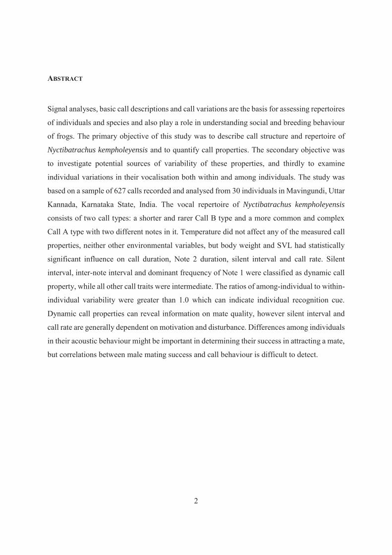
ABSTRACT
Signal analyses, basic call descriptions and call variations are the basis for assessing repertoires
of individuals and species and also play a role in understanding social and breeding behaviour
of frogs. The primary objective of this study was to describe call structure and repertoire of
Nyctibatrachus kempholeyensis and to quantify call properties. The secondary objective was
to investigate potential sources of variability of these properties, and thirdly to examine
individual variations in their vocalisation both within and among individuals. The study was
based on a sample of 627 calls recorded and analysed from 30 individuals in Mavingundi, Uttar
Kannada, Karnataka State, India. The vocal repertoire of Nyctibatrachus kempholeyensis
consists of two call types: a shorter and rarer Call B type and a more common and complex
Call A type with two different notes in it. Temperature did not affect any of the measured call
properties, neither other environmental variables, but body weight and SVL had statistically
significant influence on call duration, Note 2 duration, silent interval and call rate. Silent
interval, inter-note interval and dominant frequency of Note 1 were classified as dynamic call
property, while all other call traits were intermediate. The ratios of among-individual to within-
individual variability were greater than 1.0 which can indicate individual recognition cue.
Dynamic call properties can reveal information on mate quality, however silent interval and
call rate are generally dependent on motivation and disturbance. Differences among individuals
in their acoustic behaviour might be important in determining their success in attracting a mate,
but correlations between male mating success and call behaviour is difficult to detect.
3
TABLE OF CONTENTS ABSTRACT .................................................................................................................................. 2
1. INTRODUCTION ................................................................................................................... 4
2. MATERIALS AND METHODS ................................................................................................ 7
2.1 Study area .................................................................................................................... 8
2.3 Data collection........................................................................................................... 11
2.4 Acoustic analysis ....................................................................................................... 14
2.5 Statistical analysis ..................................................................................................... 15
3. RESULTS ........................................................................................................................... 16
3.1 Call structure ............................................................................................................. 16
3.2 Influence of temperature and body size on call structure .......................................... 19
3.3 Individual variation in call structure ......................................................................... 22
4. DISCUSSION ...................................................................................................................... 23
4.1 Call structure ............................................................................................................. 23
4.2 Influence of temperature and body size on call structure .............................................. 25
4.3 Individual variation in call structure ......................................................................... 26
5. REFERENCES ..................................................................................................................... 29
APPENDIX ................................................................................................................................. 32
4
1. INTRODUCTION
The estimated number of species on Earth varies between 7.4 and 10 million (Mora et
al. 2011). Of these, 7658 are amphibians (AmphibiaWeb 2017), but the number of new species
is increasing rapidly due to an intensified effort of exploration (Aravind & Gururaja 2011). In
addition, species are recognised based on the use of molecular tools in integrated taxonomic
surveys (Vieites et al. 2009) and related comparative bioacoustic analyses.
At the same time, amphibian populations are declining and becoming extinct at an
increasing rate (Stuart et al. 2004) – well exceeding the historical background estimates
(McCallum 2007). This is due to habitat loss, degradation, fragmentation and disturbance
(Wells 2010), pollution (Sparling 2010), the chytrid fungus Batrachochytrium dendrobatidis
(Molur et al. 2015), global changes in climate and UV radiation (Collins & Storfer 2003) and
the synergistic effects of all above mentioned reasons (Vonesh et al. 2010). In general,
amphibians are sensitive to environmental change and are therefore often used as indicator taxa
(Welsh & Ollivier 1998). They are vulnerable because of their permeable skin, use of multiple
habitat, dependence on water, complex life cycles, habitat isolation and specialisation,
population structure, limited geographic range, small body size, ectothermic metabolism,
limited dispersal ability, anti-predator behaviour, and boom and bust population cycles (Wells
2010).
As a consequence, amphibian decline may have knock-on effects on other trophic levels
and thereby threaten other species, ecosystem structure and function. For example, Whiles et
al. (2006) demonstrated consequences for primary production, shifts in algal community and
consumer structure, and organic matter dynamics. This is because amphibians play diverse
roles in ecosystem functions. On the one hand by – tadpoles - feeding on algae and
phytoplankton (Crump 2009; Wells 2010). On the other hand, amphibians serving as prey for
several species, for example snakes, other anurans, birds, aquatic insects, snails, fishes and
small mammals (Aravind & Gururaja 2011; Wells 2010). Furthermore, amphibians also have
economic relevance for humans (Aravind & Gururaja 2011; Crump 2009).
The Indian subcontinent provides home for a unique array of flora and fauna because
of its successive and long periods of isolation (Roelants et al. 2004). Over 300 amphibian
species are currently known to occur here (Dinesh et al. 2013). These include frogs and toads,
caecilians and salamanders, portraying high-level endemism particularly in the Eastern
5
Himalayas and the Western Ghats (Roelants et al. 2004). The Western Ghats mountains are
classed as a biodiversity hotspot (Myers et al. 2000), where more than 92% of the known 225
amphibian species are endemic (Garg et al. 2017), but diversity may be severely
underestimated in this region (Biju et al. 2014). The high level of endemism is perhaps a result
of the discontinuity in the mountain chain that restricts dispersal (Naniwadekar & Vasudevan
2007). The endemic species are confined to the rainforests and include the genera Ghatophryne,
Xanthophryne, Micrixalus, Melanobatrachus, Ramanella, Nasikabatrachus, Nyctibatrachus,
Indirana, Ghatixalus and Raorchestes. The families Dicroglossidae, Rhacophoridae and
Nyctibatrachidae account for 50% of the total species richness in the Western Ghats (Aravind
& Gururaja 2011).
The Nyctibatrachidae family evolved between the Cretaceous and Palaeocene,
coinciding with the time that the Indian sub-continent was isolated from Gondwana (Van
Bocxlaer et al. 2012). It consists of the genus Lankanectes, confined to Sri Lanka and the genus
Nyctibatrachus endemic to the Western Ghats (Van Bocxlaer et al. 2012). The family today
contains 36 known species (Garg et al. 2017; Krutha et al. 2017). The first Nyctibatrachus
species, or Night Frog species as they are commonly known (Garg et al. 2017), was described
in 1882 by Boulenger and its taxonomy was revised recently by Biju et al. (2011) . The
distribution of Night Frogs stretches through the Western Ghats, from northern Maharashtra to
Tamil Nadu in the south (Biju 2011). They are associated with torrent mountain streams most
of the time (Aravind & Gururaja 2011), but they can also be found in leaf litter (Priti et al.
2015). Their size (snout-vent length) vary between 10 and 77 mm and they can be identified
by their brownish dorsal colour, glandular wrinkled skin, rhomboid pupil, notched tongue and
pointed vomerine teeth (Biju 2011).
Anuran reproductive modes vary widely and exhibit unique features between species.
This diversity, with forty distinctive reproductive modes, is due to environmental, evolutionary
and ecological selective pressures (Aravind & Gururaja 2011). A common categorisation
incorporates the different modes of egg deposition (sites) and tadpole development. In addition,
there are variations in fertilisation mode (external or internal), in amplexus (inguinal, axillary,
cephalic or the lack of it), in egg and clutch size and in reproductive effort (Wells 2010). In
tropical regions, many anurans breed throughout the long rainy season, some even all year
round, but with varying intensity depending on the rainfall (Wells 2010).
6
Active partner choice by females is a process where females assess and select males
with the most attractive characteristics, i.e. the ones offering the most benefits. The direct
benefits increase the reproductive performance of females via access to resources (e.g. high
quality oviposition sites) possessed by the male, by parental care or choosing the most fertile
male. They also avoid disease - or parasite - infected males, and by selecting males that can be
easily located, they reduce search time, and predation risk. The indirect benefits include traits
that increase the genetic quality of the offspring (Wells 2010).
Females may base their choices of partner on resource quality, size, parental care,
chemical cues or calling activity. Females can also select mates on the basis of physical traits
such as male size. This may indicate certain fitness-related traits in the offspring, for example
higher survival or faster growth rates. In a wider context, territory quality and parental care
assessment can also be considered as visual cues. When males defend oviposition sites and
these vary in quality, it is possible that females chose mate on this basis, although male size
and territory quality can be correlated (Wells 2010).
Calling activity or vocalisation, is a sort of information transfer that is practiced by
several animals from insects to whales (Badrinath & Gururaja 2012). Amphibians produce a
wide range of sounds depending on the context, so it can signal distress cause by a predator,
warning, release (from the grip of another male), territory boundary, and advertisement. Calling
behaviour and call characteristics of males are important in mate attraction, female mate choice
and male mating success in frogs (Pröhl 2003). Each species have distinctive ‘singing’, and
advertisement calls can happen in a chorus or individually. Reproductive calls are the most
commonly encountered, mostly emitted by males during the breeding season. Advertisement
calls typically have two functions: attracting mates and signalling territorial information to
conspecifics (Koehler et al. 2017).
Basic call descriptions and their variations play a role in understanding the social and
breeding behaviour of frogs (Hopp et al. 2012). These variations can occur at different levels,
namely within individuals, between individuals in the same population, and between
individuals of separate populations. Acoustic divergence within and between individuals could
be influenced by male motivation, which in turn can depend upon external (e.g. environmental
impacts) and internal factors. Variation can be expected to be the lowest within individuals,
then between individuals of the same population, and the most between individuals of different
7
populations (Koehler et al. 2017). In addition, bioacoustic variations among individuals might
offer cues for females’ choice (Gambale et al. 2014). On the within-individual level, the less
variable (static) call properties might mean species recognition and individual identity, whereas
the more dynamic call traits inform about mate quality and directional female preferences
(Gerhardt 1991).
As above mentioned, environmental and morphologic factors often influence calling
behaviour. Temperature, for instance regulates the vocal activity period and the characteristics
of calls, whereas body size is generally strongly correlated with the dominant frequency of
signals. This means that smaller frogs emit higher frequency calls because of their shorter vocal
cords (Koehler et al. 2017).
Kempholey Night Frogs (Nyctibatrachus kempholeyensis) are abundant and can be
found in the torrent streams of evergreen and semi-evergreen forests as well as at shaded edges
of agricultural areas. This small sized nocturnal species occupy semi-aquatic and aquatic
habitats where they mainly breed along the shallow stream edges and slow-flowing waters.
They display nocturnal breeding activity and courtship behaviour in the form of advertisement
calls (Gururaja 2012).
Although Nyctibatrachus species are relatively well-studied in terms of morphological
descriptions, genetic relationships and natural history (Garg et al. 2017), research on
behavioural aspects, vocal repertoires, call structure and intraspecific variation are relatively
few. The basic call structure of Nyctibatrachus kempholeyensis was described by Gururaja et
al. (2014) examining call duration and dominant frequency mainly for comparative purposes
with Nyctibatrachus kumbara and Nyctibatrachus jog species. This study attempts to provide
a more detailed acoustic description in other call properties, as well as examining individual
differences to know more about their role as a female attractant among males.
Therefore, the primary objective of this study was to describe the call structure of
N.kempholeyensis. I also investigate potential sources of variability of call properties, such as
body size and temperature, and examine within- and among-individual variations in
vocalisation.
2. MATERIALS AND METHODS

8
2.1 Study area
The study area was located in the Southwest coastal region of India, within the central
Western Ghats mountain range in the Sharasvathi River basin (Fig.1). This wet hilly region has
tropical monsoon climate coming from southwest which begins in June and lasts up to
November with a mean annual rainfall of c. 7500 mm. High humidity, continuous cloud cover
and mostly quiet winds characterize the wet season and the region in general. The temperature
varies between 21 and 26°C during the season.
Rice paddy fields and Areca nut plantations intermit the natural vegetation of dense
tropical evergreen rainforest ecosystem that provides home for diverse flora and fauna, many
of which are endemic.
Figure 1: Location of the study site in the Western Ghats mountains on the Indian sub-continent (insert)mand the
local placement of the study area within Siddapur region of Karnataka State
The study took place at two sites close to Mavingundi, which is a small hamlet of
Kodkani village, in Siddapur subdivision, in Uttar Kannada District of Karnataka State, India.
The study sites are part of the down streams of Sharavathi River catchment and consist of a
matrix of evergreen forests, Areca palm plantations and paddy fields. The first site (14.25204-
9
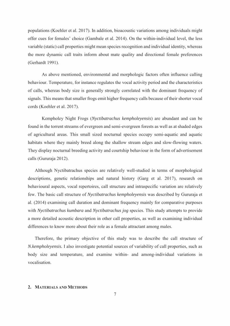
14.25291°N, 74.80120-74.80210°E, 541 m above sea level) is located in small areas of
uncultivated and cultivated Areca plantations (c. 200 m²) and uncultivated rice fields that are
currently used as grazing land for cattle and buffalos (Fig.2A). Rice cultivation began about 90
years ago and lasted until 1991 (personal communication with Ashok Hegde). Kempholey
Night Frogs can be found along the shaded edges of abandoned paddy fields, Areca gardens,
and along the stream.
The second site (14.25541-14.25715°N, 74.80612-74.80703°E, 602 m above sea level)
is located north of the Mavingundi Falls and consists of forest, streams and a power line
clearing (Fig.2B). For the power line (at the north end of the site) trees were cut about 60-65
years ago and this small patch is occasionally used for grazing. There is a small dam at the
southern end where the stream is diverted towards the hamlet for drinking purposes (personal
communication with Ashok Hegde). The status of the forest is Reserved Forest with minor
forest use such as honey and fruit (Garcinia gummigutta, Artocarpus gomezianus) extraction
(personal communication with forest guards in Mavingundi).
Figure 2: Map of the study sites with the two sites at Mavingundi.
2.2 Study species
Three Night Frog species are found at Mavingundi, namely N. jog, N. kumbara and N.
kempholeyensis. The latter were chosen for this study because they are more widely distributed
A
B
10
in the study area compared to the two other species, however they are the least easily detectable
due to their smaller size.
Nyctibatrachus kempholeyensis is distributed in streams at Jog falls, Someshwar,
Kempholay, Muthodi and Kemmanagundi in Karnataka, and at Banasura and Suganthagiri in
Kerala (Biju 2011). The breeding and adult habitat of the species is confined to perennial
streams and shallow water - both of which are filled with leaf litter and organic mulch – in
evergreen and semi-evergreen forest. These nocturnal frogs can be found on and under low
vegetation, organic litter and small rocks and stones.
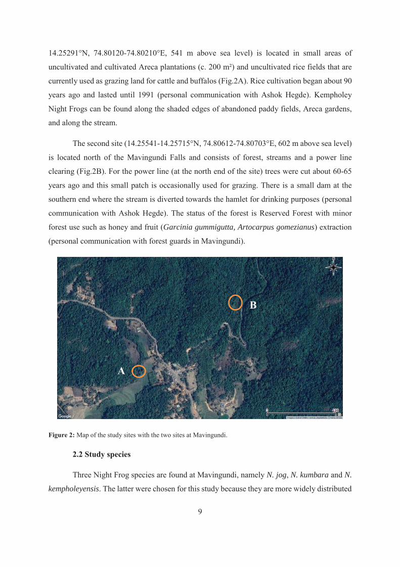
Figure 3: Photo of Lali (SVL: 19.67 mm; weight: 1.59 g).
Species identification was based on the following physical characteristics: average size
18-26 mm, ‘square’ appearance of glandular folds on dorsum, rhombus and horizontal pupil,
Y shaped ridge on snout (Gururaja 2012) (Fig.3), males secondary sexual characters based on
11
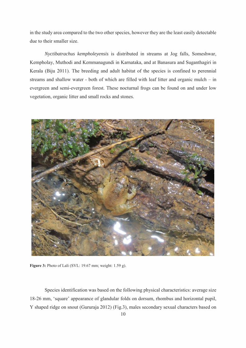
their yellowish femoral gland and pared lateral vocal sacs in whitish colour (Fig.4) and females
lay relatively large pigmented eggs (1.2 ± 0.4 mm) (Biju 2011).
Figure 4: Photo of Tommy with laterally inflated vocal sacs during calling. (Measurement were not taken.)
2.3 Data collection
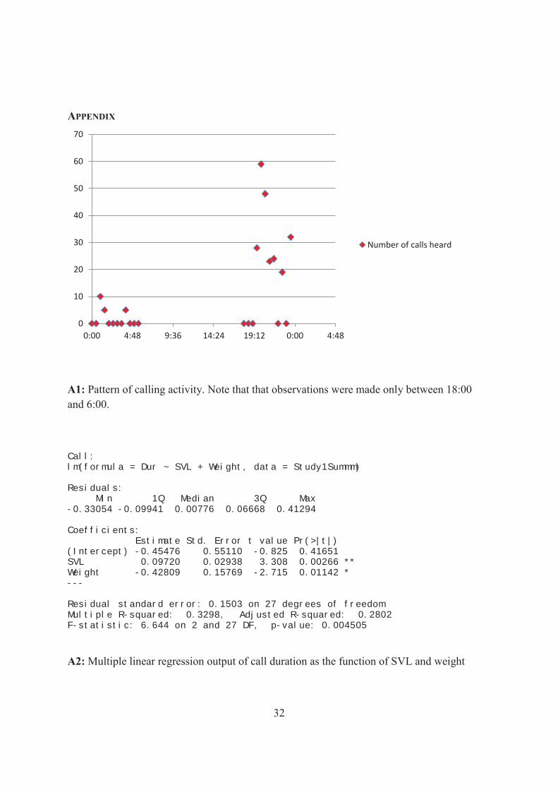
A preliminary study determined the peak activity period by temporal mapping of frogs with
observations every half an hour from 18:00 to 6:00. Calls were occasionally heard during
daytime from shaded parts of paddy, Areca plantation and forest edges, but calling generally
started at 19:00 and peaked between 20:00 and 24:00. The call activity pattern is presented in
Appendix 1. Similarly, spatial mapping was done in three different 100x100m quadrats. Within
these quadrats, 10x10m quadrats were randomly selected and visited to assess N.
kempholeyensis distribution. At each sample site, 10 minutes were spent detecting frogs. GPS
coordinates and elevation data were provided by Garmin Etrex 30.

12
Figure 5: Photo of Luke with 2 clutches of eggs. (Measurements were not taken.)
Mating behaviour begins with advertisement calls of the male when the paired vocal sac
inflats along their side (Fig. 4). After the female approaches the male, he mounts and grasps
her by the arm pits forming axillary amplexus. They remain in amplexus for about 3-5 minutes,
while they usually search for an ideal oviposition site by turning around together. Then the
female slowly releases the pigmented eggs (X̅=6.3, n=8) at average height of 8.7 cm (n=12)
and leaves. Oviposition materials varies between Indian Pandanus, black pepper leaves, other
shorter bushes, grass blades, higher stemmed plants (Fig.5), dead leaves (Fig.6) or sticks
(Fig.7). The male stays with the eggs and sometimes starts calling soon after mating. He
exhibits parental care by protecting the eggs for several days.

13
Figure 6: Photo of Kumar with a clutch of eggs on a dead leaf (SVL: 21.83 mm; weight: 1.57 g).
Figure 7: Photo by Amit Hegde of a male protecting his egg clutch. (Measurements were not taken.)

14
The subsequent study on call structure took place between 23rd of August and 9th of
September 2017. N. kempholeyensis found using a flashlight and by tracing calling males below
and on the short vegetation along the edges of streams and flowing water. Frogs typically called
from grass, bushes, dry leaves or from stones and sticks at height between ground level and 20
cm. After finding the target individual, their calling was recorded from a distance not greater
than 30 cm with a Zoom H1 recorder (in WAV format at a sampling rate of 96 kHz/24 Bit).
After this, the males were captured, the snout-vent length (SVL) measured with a digital vernier
calliper (Powerfix) and weight measured with a small digital balance (GuanHeng) for the
purpose of examining the influence of these morphometric traits on call properties. Strong site
tenacity of territorial males allowed reliable individual identification, but to exclude the
possibility of double-sampling, dorsal photos of the frogs were also taken. This reveals
individual differences in a non-invasive manner. These measurements did not last longer than
5 minutes, and frogs were immediately released. In total, thirty individual males were recorded
and measured.
In addition, other measurements were also recorded in order to investigate their
influence on the call properties. They are the following: weather condition (light rain/no rain);
lunar cycle (waxing crescent/first quarter/waxing gibbous/full moon/waning gibbous); air
temperature and relative humidity (by using Brunton ADC Pro digital thermo-hygrometer). On
the following days the estimation of canopy cover (crown closure) took place at the breeding
site using Glama android application.
Furthermore, individual male observations took place between the 11th and 30th of
September (2017), by visiting eight individuals three consecutive days for clutch height, clutch
size and behavioural activity observations.
2.4 Acoustic analysis
Call recordings were imported to the audio analysis software, Raven Pro 1.4, a
commonly used tool for biological sound measuring, analysis and illustration (Koehler et al.
2017). The call structure analysis was based on the note-centred approach. From the waveform
display (oscillogram), temporal measurements were quantified, such as call duration, note
duration, call rate, note repetition rate, silent interval, and inter-note interval. From the
15
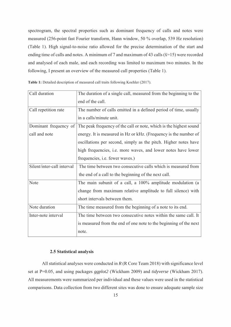
spectrogram, the spectral properties such as dominant frequency of calls and notes were
measured (256-point fast Fourier transform, Hann window, 50 % overlap, 539 Hz resolution)
(Table 1). High signal-to-noise ratio allowed for the precise determination of the start and
ending time of calls and notes. A minimum of 7 and maximum of 43 calls (x̅=15) were recorded
and analysed of each male, and each recording was limited to maximum two minutes. In the
following, I present an overview of the measured call properties (Table 1).
Table 1: Detailed description of measured call traits following Koehler (2017).
Call duration The duration of a single call, measured from the beginning to the
end of the call.
Call repetition rate The number of calls emitted in a defined period of time, usually
in a calls/minute unit.
Dominant frequency of
call and note
The peak frequency of the call or note, which is the highest sound
energy. It is measured in Hz or kHz. (Frequency is the number of
oscillations per second, simply as the pitch. Higher notes have
high frequencies, i.e. more waves, and lower notes have lower
frequencies, i.e. fewer waves.)
Silent/inter-call interval The time between two consecutive calls which is measured from
the end of a call to the beginning of the next call.
Note The main subunit of a call, a 100% amplitude modulation (a
change from maximum relative amplitude to full silence) with
short intervals between them.
Note duration The time measured from the beginning of a note to its end.
Inter-note interval The time between two consecutive notes within the same call. It
is measured from the end of one note to the beginning of the next
note.
2.5 Statistical analysis
All statistical analyses were conducted in R (R Core Team 2018) with significance level
set at P=0.05, and using packages ggplot2 (Wickham 2009) and tidyverse (Wickham 2017).
All measurements were summarized per individual and these values were used in the statistical
comparisons. Data collection from two different sites was done to ensure adequate sample size
16
and to avoid spatial autocorrelation. (Site was included in the statistical analyses as an
independent variable, however comparison was not done between them.)
As calling is an energetically expensive activity, it is dependent on temperature due to
the ectothermic nature of frogs. Environmental temperature can influence the characteristics of
vocal signals, in particular the temporal features (Koehler et al. 2017). Similarly, body size
(SVL) can highly correlate with certain call traits, particularly with dominant frequency
(reviewed in Wells 2010). Therefore the association between air temperature, body size, body
mass, weather condition, lunar phase, canopy cover, site and acoustic features were examined
using multiple regression analysis. For each call trait, environmental and morphological factors
were included as independent variables. In addition, stepwise regression analyses with
‘backward’ method were also conducted that reduced variables until only the significant ones
are left in order to eliminate masking effects.
To assess call variability within and among individuals, coefficients of variations
(CV=100%*SD/X̅) were calculated. Within-male coefficients of variation (CVw) were based
on the mean and standard deviation of each call properties for each male. To distinguish
between static and dynamic traits, Gerhardt (1991) suggested that CV values less than 5% are
static, and CV values more than 12% are dynamic traits. The values between 5 and 12% are
considered intermediate (Gerhardt 1991). Among-individual coefficient of variation (CVa)
were calculated from the grand mean and standard deviation based on the average values of
individuals (Gasser et al. 2009). The ratio of among-individual and within-individual variation
was determined as CVa /CVw in order to see variability among males. If the CVa /CVw ratio is
> 1 for a given call property, it is relatively more variable among individuals and it might
function as individual recognition cue (Bee et al. 2001; Jouventin et al. 1999).
3. RESULTS
3.1 Call structure
Kempholey Night Frog males produced two distinctive call types during their
advertisement calls: a common Call A type (Fig.9 and 10), and a rarer and much shorter Call
B type (Fig.8). Call A (Fig.9 and 10) consists of multiple notes per call and is a complex call
because it contains two different note types. These notes are organised into one initial note of
17
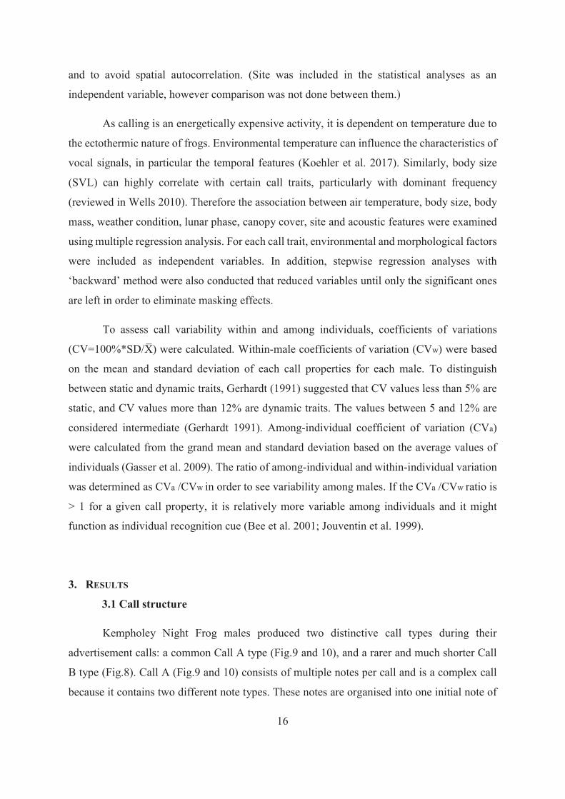
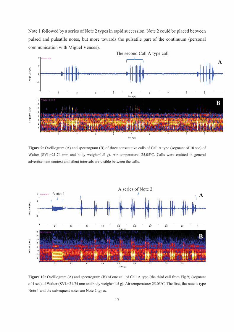
Note 1 followed by a series of Note 2 types in rapid succession. Note 2 could be placed between
pulsed and pulsatile notes, but more towards the pulsatile part of the continuum (personal
communication with Miguel Vences).
Figure 9: Oscillogram (A) and spectrogram (B) of three consecutive calls of Call A type (segment of 10 sec) of
Walter (SVL=21.74 mm and body weight=1.5 g). Air temperature: 25.05ºC. Calls were emitted in general
advertisement context and silent intervals are visible between the calls.
Figure 10: Oscillogram (A) and spectrogram (B) of one call of Call A type (the third call from Fig.9) (segment
of 1 sec) of Walter (SVL=21.74 mm and body weight=1.5 g). Air temperature: 25.05ºC. The first, flat note is type
Note 1 and the subsequent notes are Note 2 types.
A
B
A
B
The second Call A type call
Note 1 A series of Note 2

18
Call B type is a simple call, which sounds like whining, consisting only one note type
within the call. Its mean duration is 0.49 second, its average call rate is 11.5/minute and its
mean dominant frequency is 3410 Hz (Table 2). They were emitted in rapid succession with
average an silent interval of 1.29 seconds, but only by three males (the analysis was based on
168 calls). They were often followed by Call A types (after about 3-15 call of Call B). These
calls were heard when another male was close-by. Its further examination is outside the scope
of this study.
Figure 8: Oscillogram (A) and spectrogram (B) of three consecutive calls of Call B type (segment of 5 sec) of
Chris (SVL=19.21 mm and body weight=1.34 g). Air temperature: 22.65ºC. Calls were emitted in general
advertisement context and silent intervals are visible between the calls.
Spectral and temporal call features are given in Table 2. The two call types mainly
differed in call duration and call repetition rate. The mean call duration of Call A (X̅=0.89 s)
was almost double of Call B (X̅=0.49 s), while the mean call repetition rate (in min/call) of
Call B (X̅=11.5) was much higher than Call A (X̅=3.9). However, dominant frequencies of the
two types of calls were similar (Call A: X̅=3489 Hz and Call B: X̅=3410).
A
B
The second Call B type call

19
Table 2: Descriptive statistics of Call A and Call B properties based on mean individual values of 30 and 3
Nyctibatrachus kempholeyensis males at Mavingundi, Uttar Kannada, Karnataka State, India. Air temperature
variation was between 20.8 and 25.6°C.
Call A Call B
Call properties X̅ ± SD Range (n=30) X̅ ± SD Range (n=3) Call duration (s) 0.89 ± 0.18 0.45-1.41 0.49 ± 0.003 0.491 -0.498 Note 1 duration (s) 0.06 ± 0.01 0.04 – 0.07 ̶̶ ̶̶ Note 2 duration (s) 0.71 ± 0.17 0.25 – 1.19 ̶̶ ̶̶ Silent interval (s) 11.87 ± 6.23 2.28 – 24.72 1.29 ± 0.46 0.76 – 1.58 Inter-note interval (s) 0.12 ± 0.03 0.07 – 0.21 ̶̶ Call repetition rate 3.9 ± 2.3 1.3 – 11.5 11.5 ± 5.8 4.8 – 15 Note repetition rate 7.6 ± 1.8 2.8 – 12.2 ̶̶ ̶̶ Call dominant frequency (Hz) 3489 ± 410 2150 – 4018 3410 ± 1037 2694 – 4599 Note 1 dominant frequency (Hz) 2943 ± 550 1755 – 3799 ̶̶ ̶̶ Note 2 dominant frequency (Hz) 3495 ± 382 2150 – 4018 ̶̶ ̶̶
3.2 Influence of temperature and body size on call structure
The mean temperature was 23.7 ºC across recordings and ranged between 20.8 and
25.6°C. By exploring the data, a positive relationship was found between air temperature and
call duration, Note 2 duration and Note 2 rate. The relationship between temperature and
dominant frequency of Note 1 was negative, while there was no linear relationship between
Note 1 duration, call rate, call and Note 2 dominant frequency, silent interval and inter-note
interval.
Males ranged in body size between 18.2 mm and 22.6 mm SVL (X̅ ± SD=20.4 ± 1 mm,
n=30) and from 1.1 g to 2 g (X̅ ± SD=1.5 g ± 0.2 g, n=30). Since these two morphometric
variables correlated by only 0.39, both of them were included in the statistical analyses. A
positive relationship was found between SVL and call rate, while SVL exhibited a negative
relationship with call duration, Note 2 duration, Note 2 rate and inter-note interval. No
relationship was found between SVL and dominant frequencies, Note 1 duration and silent
interval. Weight negatively related to silent interval and inter-note interval, and positively
related to durations of call and notes, dominant frequencies (both of call and of the two note
types), call and Note 2 rate.

20
In addition, canopy cover exhibited positive relationship with Note 1 duration,
dominant frequency of call and Note 2 and with inter-note interval. It negatively related to
dominant frequency of Note 1 and silent interval, while there was no relationship between call
and Note 2 duration, call and Note 2 rate.
Table 3 shows the results of the multiple linear regression models where all variables
(temperature, SVL, weight, weather condition, lunar phase, canopy cover and site) were
included. Of all variables, only body weight had a significant effect on call properties of call
duration (R²= 0.6379, F= 4.69, P= 0.0481), silent interval (R²= 0.4445, F= 8.0436, P= 0.0132),
call rate (R²= 0.3971, F= 5.4704, P= 0.0347) and Note 2 duration (R²= 0.5557, F= 4.1964, P=
0.0597). The other call traits were statistically unaffected by all measured variables.
The multiple linear stepwise regression models showed significant effect of SVL and
body mass on call duration (R²= 0.3298, F= 5.9169, P= 0.0219, β= 0.097 for SVL and F=
7.3703, P= 0.01142, β= - 0.428 for weight)(A2), on Note 2 duration (R²= 0.3198, F= 5.1473,
P= 0.03149, β= 0.092 for SVL and F= 7.5493, P= 0.01056, β= - 0.428 for weight)(A3), and on
Note 2 rate (R²= 0.2656, F= 6.5611, P= 0.01632, β= 0.814 for SVL and F= 6.5611, P= 0.0163,
β= - 4.211 for weight)(A3). Call rate (R²= 0.2522, F= 9.4408, P= 0.00469, β= 15.61)(A5) and
silent interval (R²= 0.2331, F-value= 8.5093, P-value= 0.00689, β= - 5.969)(A6) was also
significantly influenced by body mass: where there was a negative relationship between body
mass and call rate, while the relationship was positive between body mass and silent interval.
Of the measured environmental and morphometric factors, none of them showed significant
effect on call properties. The output of these regression models is found in the Appendix (A2-
A6).

Tab
le 3
: Sum
mar
y of
stat
istic
al te
sts i
nclu
ding
all
varia
bles
to e
stim
ate
tem
pera
ture
, SV
L, w
eigh
t, ca
nopy
cov
er, l
unar
pha
se, w
eath
er c
ondi
tion
and
site
effe
cts o
n ca
ll pr
oper
ties o
f Cal
l A ty
pe in
Nyc
tibat
rach
us k
emph
oley
ensi
s. C
D: C
all d
urat
ion
(s);
SI: S
ilent
inte
rval
(s);
CR
: Cal
l rat
e (m
in/c
all);
N1D
: Not
e 1
dura
tion
(s);
N2D
: Not
e 2
dura
tion
(s);
II: I
nter
-not
e in
terv
al (s
); N
2R: N
ote
2 re
petit
ion
rate
(min
/not
e); C
DF:
Dom
inan
t fre
quen
cy o
f cal
l (H
z); N
1F: D
omin
ant f
requ
ency
of N
ote
1 (H
z); N
2F:
Dom
inan
t fre
quen
cy o
f Not
e 2
(Hz)
. Bol
d ty
pe in
dica
tes s
tatis
tical
sign
ifica
nce.
Tem
pera
ture
SV
L W
eigh
t C
anop
y co
ver
Luna
r pha
se
Wea
ther
Si
te
Cal
l pr
oper
ties
r²- valu
e F- valu
e P- valu
e F- valu
e P- valu
e F- valu
e P- valu
e F- valu
e P- valu
e F- valu
e P- valu
e F- valu
e P- valu
e F- valu
e P- valu
e C
D
0.63
79
3.13
86
0.09
82
3.98
21
0.06
58
4.69
00
0.04
81
1.89
27
0.19
05
2.70
18
0.07
38
0.12
58
0.72
81
0.02
15
0.88
54
SI
0.44
45
0.13
56
0.71
82
0.00
34
0.95
42
8.04
36
0.01
32
0.11
27
0.74
20
0.09
02
0.98
40
1.07
32
0.31
78
1.47
28
0.24
50
CR
0.
3971
0.
5647
0.
4648
0.
7735
0.
3940
5.
4704
0.
0347
0.
0001
0.
9942
0.
5858
0.
6782
0.
0673
0.
7991
0.
0011
0.
9742
N
1D
0.21
83
0.04
71
0.83
12
0.05
59
0.81
66
0.35
76
0.55
94
0.34
39
0.56
69
0.52
84
0.71
69
0.22
89
0.63
97
0.76
35
0.39
70
N2D
0.
5557
2.
4826
0.
1374
2.
9543
0.
1077
4.
1964
0.
0597
0.
0014
0.
9705
1.
9525
0.
1575
0.
0492
0.
8277
0.
0165
0.
8997
II
0.
3418
0.
0073
0.
9330
0.
1614
0.
6939
0.
3254
0.
5774
0.
8492
0.
3724
1.
3486
0.
3010
0.
4500
0.
5133
0.
0824
0.
7782
N
2R
0.46
49
0.84
96
0.37
23
2.92
44
0.10
93
3.65
85
0.07
65
0.01
00
0.92
17
0.93
75
0.47
07
0.04
87
0.82
86
0.92
22
0.35
32
CD
F 0.
2362
0.
0313
0.
8621
0.
0183
0.
8942
0.
3928
0.
5409
1.
4033
0.
2559
0.
2309
0.
9164
1.
5343
0.
2358
0.
0254
0.
8757
N
1DF
0.25
60
0.08
61
0.77
35
0.00
03
0.98
57
0.25
79
0.61
95
0.36
09
0.55
76
0.81
63
0.53
57
0.82
94
0.37
79
0.01
73
0.89
71
N2D
F 0.
2465
0.
0479
0.
8299
0.
0026
0.
9604
0.
3550
0.
5608
1.
4434
0.
2495
0.
3076
0.
8681
1.
4984
0.
2411
0.
0016
0.
9683
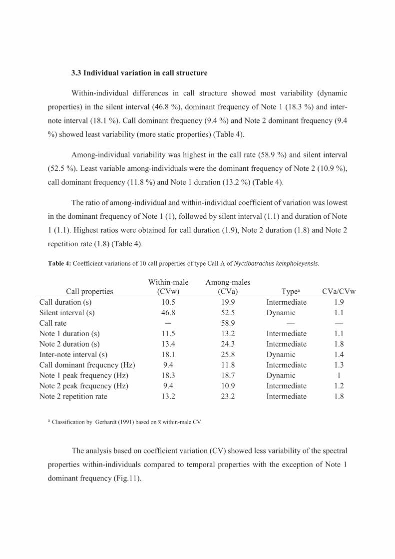
3.3 Individual variation in call structure
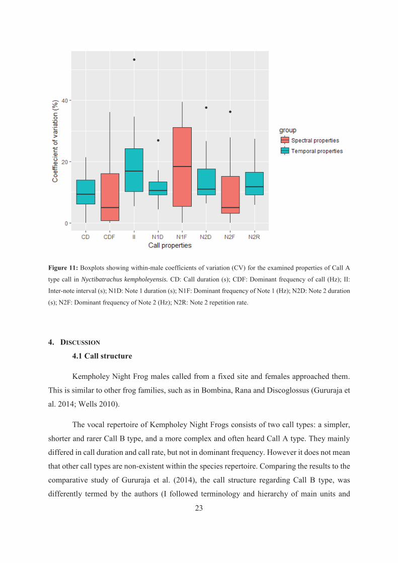
Within-individual differences in call structure showed most variability (dynamic
properties) in the silent interval (46.8 %), dominant frequency of Note 1 (18.3 %) and inter-
note interval (18.1 %). Call dominant frequency (9.4 %) and Note 2 dominant frequency (9.4
%) showed least variability (more static properties) (Table 4).
Among-individual variability was highest in the call rate (58.9 %) and silent interval
(52.5 %). Least variable among-individuals were the dominant frequency of Note 2 (10.9 %),
call dominant frequency (11.8 %) and Note 1 duration (13.2 %) (Table 4).
The ratio of among-individual and within-individual coefficient of variation was lowest
in the dominant frequency of Note 1 (1), followed by silent interval (1.1) and duration of Note
1 (1.1). Highest ratios were obtained for call duration (1.9), Note 2 duration (1.8) and Note 2
repetition rate (1.8) (Table 4).
Table 4: Coefficient variations of 10 call properties of type Call A of Nyctibatrachus kempholeyensis.
Call properties Within-male
(CVw) Among-males
(CVa) Typeᵃ CVa/CVw Call duration (s) 10.5 19.9 Intermediate 1.9 Silent interval (s) 46.8 52.5 Dynamic 1.1 Call rate — 58.9 — — Note 1 duration (s) 11.5 13.2 Intermediate 1.1 Note 2 duration (s) 13.4 24.3 Intermediate 1.8 Inter-note interval (s) 18.1 25.8 Dynamic 1.4 Call dominant frequency (Hz) 9.4 11.8 Intermediate 1.3 Note 1 peak frequency (Hz) 18.3 18.7 Dynamic 1 Note 2 peak frequency (Hz) 9.4 10.9 Intermediate 1.2 Note 2 repetition rate 13.2 23.2 Intermediate 1.8
ᵃ Classification by Gerhardt (1991) based on x̅ within-male CV.
The analysis based on coefficient variation (CV) showed less variability of the spectral
properties within-individuals compared to temporal properties with the exception of Note 1
dominant frequency (Fig.11).
23
Figure 11: Boxplots showing within-male coefficients of variation (CV) for the examined properties of Call A
type call in Nyctibatrachus kempholeyensis. CD: Call duration (s); CDF: Dominant frequency of call (Hz); II:
Inter-note interval (s); N1D: Note 1 duration (s); N1F: Dominant frequency of Note 1 (Hz); N2D: Note 2 duration
(s); N2F: Dominant frequency of Note 2 (Hz); N2R: Note 2 repetition rate.
4. DISCUSSION
4.1 Call structure
Kempholey Night Frog males called from a fixed site and females approached them.
This is similar to other frog families, such as in Bombina, Rana and Discoglossus (Gururaja et
al. 2014; Wells 2010).
The vocal repertoire of Kempholey Night Frogs consists of two call types: a simpler,
shorter and rarer Call B type, and a more complex and often heard Call A type. They mainly
differed in call duration and call rate, but not in dominant frequency. However it does not mean
that other call types are non-existent within the species repertoire. Comparing the results to the
comparative study of Gururaja et al. (2014), the call structure regarding Call B type, was
differently termed by the authors (I followed terminology and hierarchy of main units and
24
subunits proposed by Koehler et al. (2017)) Their longer Call B duration (X̅=11.69 sec) and
lower dominant frequency (X̅=1633.67 Hz) is due to an analysis that would comply with a call
group of a series of Call B type, followed by one Call A type. Since there are silent intervals in
between, the dominant frequency is consequently lower. The common Call A type was
similarly described regarding the call structure, and its duration is comparable to the results
here (X̅=0.517 sec compared to X̅=0.89 sec here), albeit a bit shorter. When comparing the call
structure of N.kempholeyensis to other Nyctibatrachus species, N.Athirappillyensis produces a
somewhat similar call to Call A type of N.kempholeyensis in having 2 parts (or notes) in it.
Similarly part 1 is much shorter than part 2. The single call of N. malanari is similar to Call B
type of N.kempholeyensis (Garg et al. 2017).
According to our observations, the short, whining Call B type was heard when two
males were in close proximity, agreeing with the general experience that aggressive calls are
directed towards male competitors during close encounters. Call A has different note types and
can have multiple functions, such as attracting females and repelling males, since the receivers
of advertisement calls could be potential mates or neighbouring males. Hence the different note
types or calls with variable note types could serve different functions as Wells concluded
(2010). In addition, the complexity of calls can also vary depending on the social environment
of the male. Future playback experiments might reveal the exact functions of the two call types.
It is important to observe and report the social context in calling activity, since for
example the proximity of other males and females can influence the calling behaviour. In
addition, since advertisement calls can also advertise parental and resource qualities (e.g.
breeding site) in order to show intent to potential partners for breeding (Wells 2010), further
studies on parental care and on egg predation would be beneficial. Furthermore, in addition to
acoustic signals, mechanism of mate choice in frogs can involve pheromones (Starnberger et
al. 2013), visual signalling (Boeckle et al. 2009; Hödl & Amézquita 2001), inflations of vocal
sacs (Hirschmann & Hödl 2006), water surface waves (Walkowiak & Münz 1985), surface
vibrations (Cardoso & Heyer 1995; Hill 2001), and age (Pröhl 2003). Mate choice in frogs is
most likely to be the complex and dynamic combinations of these cues (Narins et al. 2003),
and examination of these cues could reveal more about this for females in N.kempholeyensis.
25
4.2 Influence of temperature and body size on call structure
In this study, the correlation of air temperature with temporal properties of call duration,
Note 2 duration and Note 2 rate is in line with results from previous studies (e.g. Gasser et al.
2009) as these features are linked to temperature dependent muscular contractions (Koehler et
al. 2017). According to Bee et al. (2013), call rate is often positively correlated with
temperature, while call duration is negatively related to it. However, contrary to this, call
duration was positively related to temperature, not negatively.
The results show that none of the call properties were significantly influenced by
temperature. The reason can be that the temperature range across the recordings were relatively
small (between 20.8 and 25.6°C) as in the study by Bee et al. (2013), although the range was
smaller there (18.6 and 20.4°C). Perhaps a more constant temperature throughout the days and
throughout the monsoon season in Tropical regions might be an explanation of why the
temperature did not affect call properties. Nevertheless, the energetically expensive activity of
calling and the ectothermic nature of frogs indicate that temperature can influence call
properties. Therefore it is important to report relationships between temperature and call
properties. In other studies where temperature played an important role, call properties were
corrected for its influence by averaging the temperature across recordings (Bee et al. 2010;
Gambale et al. 2014; Gasser et al. 2009; Kaefer & Lima 2012).
When other environmental variables were included in the statistical model, such as
lunar phase, weather condition, canopy cover and site, they did not influence any of the call
properties. The measurement of canopy cover might be less useful because of the different
angles and viewpoints of frogs from the ones the photos were taken from (personal
communication with KV Gururaja). In addition, regarding the lunar phase, there is no clear
proof provided in this study that the moon does not influence call performance. This is because
the study period was from between 23rd of August and 9th of September (with measurements
of environmental factors), thus it did not make up a complete lunar cycle. Nevertheless, a
literature review showed evidence that most amphibians respond to lunar phase, including
reproductive behaviour and this response is highly species specific (Grant et al. 2012).
Furthermore, regarding the weather conditions, on heavy rainy nights more calls were heard
according to our observations in July and August. However, during the study period at the end
of August and in September, rainy nights were fewer.
26
According to the findings, SVL did not relate to spectral properties, but to the temporal
properties of call rate (positively) and to call duration, Note 2 duration, Note 2 rate and inter-
note interval (negatively), while weight related to temporal (silent interval and inter-note
interval negatively) and to spectral properties (dominant frequency of notes and call, duration
of call and notes and rates of call and Note 2 positively) as well. Interestingly, call duration had
a negative linear relationship with SVL, but positively related to weight. This might indicate
the relationship between calling activity and its energy consumption, since temporal call
variables usually correlate with energy expenditure (Koehler et al. 2017).
The multiple linear regression models showed that the potential sources of variability
of call properties of call duration, Note 2 duration, Note 2 rate, call rate and silent interval were
due to SVL and body mass. Thus, it seems that morphological variables had greater influence
on some of the temporal call properties than on the spectral ones. This is in contrast to some
studies, which reported strong negative correlation of dominant frequency and body size (in
Wells 2010). However, other studies found that correlation between body size and call
properties were not present among males of the same population, but only in geographically
distant populations (in Gasser et al. 2009; in Wells 2010). For this reason, it would have been
interesting to examine the difference between the two populations of the two study sites.
The effect of both SVL and weight might indicate that these variables together can give
a better estimate than SVL alone, or possibly the use of body condition index. Body condition
index uses of residuals from a regression of body mass on a linear measure of body size
(Albrecht I. Schulte-Hostedde et al. 2005). It is important to note however, that silent intervals
and call rate are often dependent on calling motivation and disturbance (Koehler et al. 2017).
In addition to the influence of environmental and morphometric factors on call properties,
social environment can effect these features as mentioned above, but it is more difficult to
measure.
4.3 Individual variation in call structure
All examined call properties varied more among males than within males (Table 4),
hence the ratios of among-individual variability to within-individual variability (CVa/CVw)
were greater than 1.0. According to Jouventin (1999), if call traits exceed the ratio of 1 and are
27
relatively more variable among individuals, they might serve as individual recognition cues.
The high values of CVw-s of silent interval and of CVa-s of call rate and silent interval indicate
high variability both within and among individuals in these call traits. It is not surprising since
silent interval and call rate can be highly affected by disturbance and calling motivation as
already mentioned.
Three properties exhibited relatively more than average variability among males than
within males, namely call duration, Note 2 duration and Note 2 rate and hence got the highest
CVa/CVw ratios. Spectral features had lower CVa/CVw ratios compared to temporal traits
(except Note 1 duration), which indicate that temporal properties showed more variability
among males than within males compared to spectral properties.
None of the call traits showed static nature in this study, however dominant frequency
of call and Note 2 were least variable (both within- and among-individuals), albeit classified
as intermediate type. It is possible that other call properties (e.g. call rise time, call fall time,
pulse rate, which is the smallest unit of a call) might prove to be static, especially because fine
temporal call traits tend to be static, as Gerhardt (1991) proposed. The classification of
Gerhardt (1991) for distinguishing between static and dynamic call properties is based on the
relative measure of within-individual variability. On the one hand, static properties (with less
variability within individuals) are generally physically constrained features and also traits that
are important in species and individual recognition and have stabilizing or weakly directional
roles in female preference tests (Bee et al. 2013).
Dynamic properties on the other hand, show greater variability within individuals
probably due to changing environmental and social contexts. Silent interval, inter-note interval
and dominant frequency of Note 1 were classified here as dynamic traits. They might reveal
information on mate quality and hence they are a target of directional female preferences. The
spectral call property of Note 1 dominant frequency as dynamic type is relatively surprising
since frequency is generally related to body size, a physically constrained feature, as discussed
above. However, it is also possible that frogs can change ‘their pitch’ according to their social
environment as Rana catesbeiana bullfrogs do (Bee & Bowling 2002). Some of the among-
male variation of call rate can be assigned to body size and weight, that is, smaller males are
calling faster than larger ones. These results are in line with some other studies, for example in
D. pumilio described by Prohl at al. (2007). It is important to note that this classification of

28
dynamic and static type of call traits is a continuum, rather than bimodal pattern of variation
(Koehler et al. 2017). Moreover, Reinhold (2009) found that the variation increased with the
duration of the recorded and analysed calls, consequently, the influential factors increased as
well.
Females often respond to call intensity, call duration, calling rate and call complexity
and they prefer males that invest more effort in calling performance (Wells 2010). Therefore it
would be beneficial to conduct future research with acoustic playback experiments to find out
the role of whining call for example and studies on territoriality.
In conclusion, basic call descriptions and intraspecific variations play a key role in
understanding social and breeding behaviour of frogs (Bee et al. 2010) and the evolution of
frog communication systems (Bee et al. 2013). It can also provide information for conservation
efforts that rely on acoustic monitoring (Bee et al. 2010) in a non-invasive manner.
29
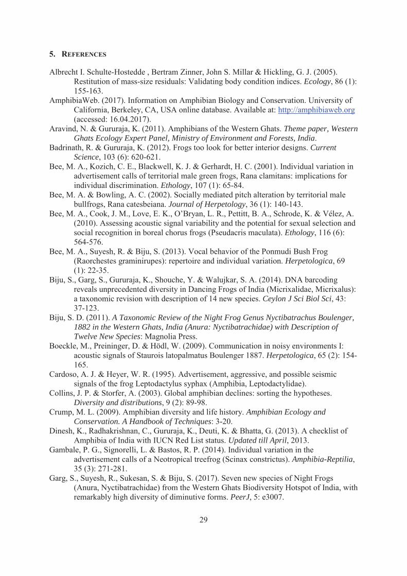
5. REFERENCES
Albrecht I. Schulte-Hostedde , Bertram Zinner, John S. Millar & Hickling, G. J. (2005). Restitution of mass-size residuals: Validating body condition indices. Ecology, 86 (1): 155-163.
AmphibiaWeb. (2017). Information on Amphibian Biology and Conservation. University of California, Berkeley, CA, USA online database. Available at: http://amphibiaweb.org (accessed: 16.04.2017).
Aravind, N. & Gururaja, K. (2011). Amphibians of the Western Ghats. Theme paper, Western Ghats Ecology Expert Panel, Ministry of Environment and Forests, India.
Badrinath, R. & Gururaja, K. (2012). Frogs too look for better interior designs. Current Science, 103 (6): 620-621.
Bee, M. A., Kozich, C. E., Blackwell, K. J. & Gerhardt, H. C. (2001). Individual variation in advertisement calls of territorial male green frogs, Rana clamitans: implications for individual discrimination. Ethology, 107 (1): 65-84.
Bee, M. A. & Bowling, A. C. (2002). Socially mediated pitch alteration by territorial male bullfrogs, Rana catesbeiana. Journal of Herpetology, 36 (1): 140-143.
Bee, M. A., Cook, J. M., Love, E. K., O’Bryan, L. R., Pettitt, B. A., Schrode, K. & Vélez, A. (2010). Assessing acoustic signal variability and the potential for sexual selection and social recognition in boreal chorus frogs (Pseudacris maculata). Ethology, 116 (6): 564-576.
Bee, M. A., Suyesh, R. & Biju, S. (2013). Vocal behavior of the Ponmudi Bush Frog (Raorchestes graminirupes): repertoire and individual variation. Herpetologica, 69 (1): 22-35.
Biju, S., Garg, S., Gururaja, K., Shouche, Y. & Walujkar, S. A. (2014). DNA barcoding reveals unprecedented diversity in Dancing Frogs of India (Micrixalidae, Micrixalus): a taxonomic revision with description of 14 new species. Ceylon J Sci Biol Sci, 43: 37-123.
Biju, S. D. (2011). A Taxonomic Review of the Night Frog Genus Nyctibatrachus Boulenger, 1882 in the Western Ghats, India (Anura: Nyctibatrachidae) with Description of Twelve New Species: Magnolia Press.
Boeckle, M., Preininger, D. & Hödl, W. (2009). Communication in noisy environments I: acoustic signals of Staurois latopalmatus Boulenger 1887. Herpetologica, 65 (2): 154-165.
Cardoso, A. J. & Heyer, W. R. (1995). Advertisement, aggressive, and possible seismic signals of the frog Leptodactylus syphax (Amphibia, Leptodactylidae).
Collins, J. P. & Storfer, A. (2003). Global amphibian declines: sorting the hypotheses. Diversity and distributions, 9 (2): 89-98.
Crump, M. L. (2009). Amphibian diversity and life history. Amphibian Ecology and Conservation. A Handbook of Techniques: 3-20.
Dinesh, K., Radhakrishnan, C., Gururaja, K., Deuti, K. & Bhatta, G. (2013). A checklist of Amphibia of India with IUCN Red List status. Updated till April, 2013.
Gambale, P. G., Signorelli, L. & Bastos, R. P. (2014). Individual variation in the advertisement calls of a Neotropical treefrog (Scinax constrictus). Amphibia-Reptilia, 35 (3): 271-281.
Garg, S., Suyesh, R., Sukesan, S. & Biju, S. (2017). Seven new species of Night Frogs (Anura, Nyctibatrachidae) from the Western Ghats Biodiversity Hotspot of India, with remarkably high diversity of diminutive forms. PeerJ, 5: e3007.
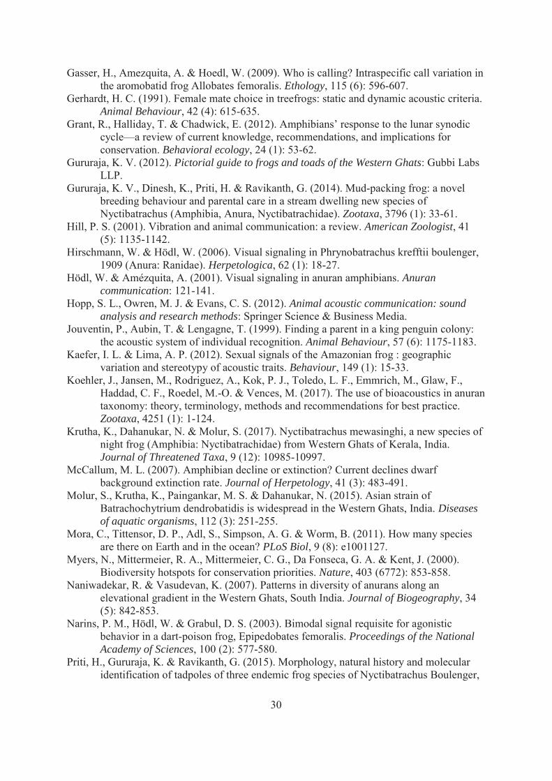
30
Gasser, H., Amezquita, A. & Hoedl, W. (2009). Who is calling? Intraspecific call variation in the aromobatid frog Allobates femoralis. Ethology, 115 (6): 596-607.
Gerhardt, H. C. (1991). Female mate choice in treefrogs: static and dynamic acoustic criteria. Animal Behaviour, 42 (4): 615-635.
Grant, R., Halliday, T. & Chadwick, E. (2012). Amphibians’ response to the lunar synodic cycle—a review of current knowledge, recommendations, and implications for conservation. Behavioral ecology, 24 (1): 53-62.
Gururaja, K. V. (2012). Pictorial guide to frogs and toads of the Western Ghats: Gubbi Labs LLP.
Gururaja, K. V., Dinesh, K., Priti, H. & Ravikanth, G. (2014). Mud-packing frog: a novel breeding behaviour and parental care in a stream dwelling new species of Nyctibatrachus (Amphibia, Anura, Nyctibatrachidae). Zootaxa, 3796 (1): 33-61.
Hill, P. S. (2001). Vibration and animal communication: a review. American Zoologist, 41 (5): 1135-1142.
Hirschmann, W. & Hödl, W. (2006). Visual signaling in Phrynobatrachus krefftii boulenger, 1909 (Anura: Ranidae). Herpetologica, 62 (1): 18-27.
Hödl, W. & Amézquita, A. (2001). Visual signaling in anuran amphibians. Anuran communication: 121-141.
Hopp, S. L., Owren, M. J. & Evans, C. S. (2012). Animal acoustic communication: sound analysis and research methods: Springer Science & Business Media.
Jouventin, P., Aubin, T. & Lengagne, T. (1999). Finding a parent in a king penguin colony: the acoustic system of individual recognition. Animal Behaviour, 57 (6): 1175-1183.
Kaefer, I. L. & Lima, A. P. (2012). Sexual signals of the Amazonian frog : geographic variation and stereotypy of acoustic traits. Behaviour, 149 (1): 15-33.
Koehler, J., Jansen, M., Rodriguez, A., Kok, P. J., Toledo, L. F., Emmrich, M., Glaw, F., Haddad, C. F., Roedel, M.-O. & Vences, M. (2017). The use of bioacoustics in anuran taxonomy: theory, terminology, methods and recommendations for best practice. Zootaxa, 4251 (1): 1-124.
Krutha, K., Dahanukar, N. & Molur, S. (2017). Nyctibatrachus mewasinghi, a new species of night frog (Amphibia: Nyctibatrachidae) from Western Ghats of Kerala, India. Journal of Threatened Taxa, 9 (12): 10985-10997.
McCallum, M. L. (2007). Amphibian decline or extinction? Current declines dwarf background extinction rate. Journal of Herpetology, 41 (3): 483-491.
Molur, S., Krutha, K., Paingankar, M. S. & Dahanukar, N. (2015). Asian strain of Batrachochytrium dendrobatidis is widespread in the Western Ghats, India. Diseases of aquatic organisms, 112 (3): 251-255.
Mora, C., Tittensor, D. P., Adl, S., Simpson, A. G. & Worm, B. (2011). How many species are there on Earth and in the ocean? PLoS Biol, 9 (8): e1001127.
Myers, N., Mittermeier, R. A., Mittermeier, C. G., Da Fonseca, G. A. & Kent, J. (2000). Biodiversity hotspots for conservation priorities. Nature, 403 (6772): 853-858.
Naniwadekar, R. & Vasudevan, K. (2007). Patterns in diversity of anurans along an elevational gradient in the Western Ghats, South India. Journal of Biogeography, 34 (5): 842-853.
Narins, P. M., Hödl, W. & Grabul, D. S. (2003). Bimodal signal requisite for agonistic behavior in a dart-poison frog, Epipedobates femoralis. Proceedings of the National Academy of Sciences, 100 (2): 577-580.
Priti, H., Gururaja, K. & Ravikanth, G. (2015). Morphology, natural history and molecular identification of tadpoles of three endemic frog species of Nyctibatrachus Boulenger,
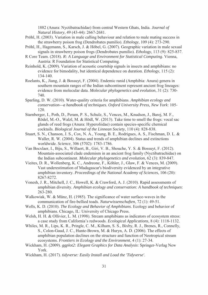
31
1882 (Anura: Nyctibatrachidae) from central Western Ghats, India. Journal of Natural History, 49 (43-44): 2667-2681.
Pröhl, H. (2003). Variation in male calling behaviour and relation to male mating success in the strawberry poison frog (Dendrobates pumilio). Ethology, 109 (4): 273-290.
Pröhl, H., Hagemann, S., Karsch, J. & Höbel, G. (2007). Geographic variation in male sexual signals in strawberry poison frogs (Dendrobates pumilio). Ethology, 113 (9): 825-837.
R Core Team. (2018). R: A Language and Environment for Statistical Computing. Vienna, Austria: R Foundation for Statistical Computing.
Reinhold, K. (2009). Variation of acoustic courtship signals in insects and amphibians: no evidence for bimodality, but identical dependence on duration. Ethology, 115 (2): 134-140.
Roelants, K., Jiang, J. & Bossuyt, F. (2004). Endemic ranid (Amphibia: Anura) genera in southern mountain ranges of the Indian subcontinent represent ancient frog lineages: evidence from molecular data. Molecular phylogenetics and evolution, 31 (2): 730-740.
Sparling, D. W. (2010). Water-quality criteria for amphibians. Amphibian ecology and conservation—a handbook of techniques. Oxford University Press, New York: 105-120.
Starnberger, I., Poth, D., Peram, P. S., Schulz, S., Vences, M., Knudsen, J., Barej, M. F., Rödel, M.-O., Walzl, M. & Hödl, W. (2013). Take time to smell the frogs: vocal sac glands of reed frogs (Anura: Hyperoliidae) contain species-specific chemical cocktails. Biological Journal of the Linnean Society, 110 (4): 828-838.
Stuart, S. N., Chanson, J. S., Cox, N. A., Young, B. E., Rodrigues, A. S., Fischman, D. L. & Waller, R. W. (2004). Status and trends of amphibian declines and extinctions worldwide. Science, 306 (5702): 1783-1786.
Van Bocxlaer, I., Biju, S., Willaert, B., Giri, V. B., Shouche, Y. S. & Bossuyt, F. (2012). Mountain-associated clade endemism in an ancient frog family (Nyctibatrachidae) on the Indian subcontinent. Molecular phylogenetics and evolution, 62 (3): 839-847.
Vieites, D. R., Wollenberg, K. C., Andreone, F., Köhler, J., Glaw, F. & Vences, M. (2009). Vast underestimation of Madagascar's biodiversity evidenced by an integrative amphibian inventory. Proceedings of the National Academy of Sciences, 106 (20): 8267-8272.
Vonesh, J. R., Mitchell, J. C., Howell, K. & Crawford, A. J. (2010). Rapid assessments of amphibian diversity. Amphibian ecology and conservation: A handbook of techniques: 263-280.
Walkowiak, W. & Münz, H. (1985). The significance of water surface-waves in the communication of fire-bellied toads. Naturwissenschaften, 72 (1): 49-51.
Wells, K. D. (2010). The Ecology and Behavior of Amphibians. Ecology and behavior of amphibians. Chicago, IL: University of Chicago Press.
Welsh, H. H. & Ollivier, L. M. (1998). Stream amphibians as indicators of ecosystem stress: a case study from California’s redwoods. Ecological Applications, 8 (4): 1118-1132.
Whiles, M. R., Lips, K. R., Pringle, C. M., Kilham, S. S., Bixby, R. J., Brenes, R., Connelly, S., Colon-Gaud, J. C., Hunte-Brown, M. & Huryn, A. D. (2006). The effects of amphibian population declines on the structure and function of Neotropical stream ecosystems. Frontiers in Ecology and the Environment, 4 (1): 27-34.
Wickham, H. (2009). ggplot2: Elegant Graphics for Data Analysis: Springer-Verlag New York.
Wickham, H. (2017). tidyverse: Easily Install and Load the 'Tidyverse'.
32
APPENDIX
A1: Pattern of calling activity. Note that that observations were made only between 18:00 and 6:00.
Call: lm(formula = Dur ~ SVL + Weight, data = Study1Summm) Residuals: Min 1Q Median 3Q Max -0.33054 -0.09941 0.00776 0.06668 0.41294 Coefficients: Estimate Std. Error t value Pr(>|t|) (Intercept) -0.45476 0.55110 -0.825 0.41651 SVL 0.09720 0.02938 3.308 0.00266 ** Weight -0.42809 0.15769 -2.715 0.01142 * --- Residual standard error: 0.1503 on 27 degrees of freedom Multiple R-squared: 0.3298, Adjusted R-squared: 0.2802 F-statistic: 6.644 on 2 and 27 DF, p-value: 0.004505
A2: Multiple linear regression output of call duration as the function of SVL and weight
0
10
20
30
40
50
60
70
0:00 4:48 9:36 14:24 19:12 0:00 4:48
Number of calls heard
33
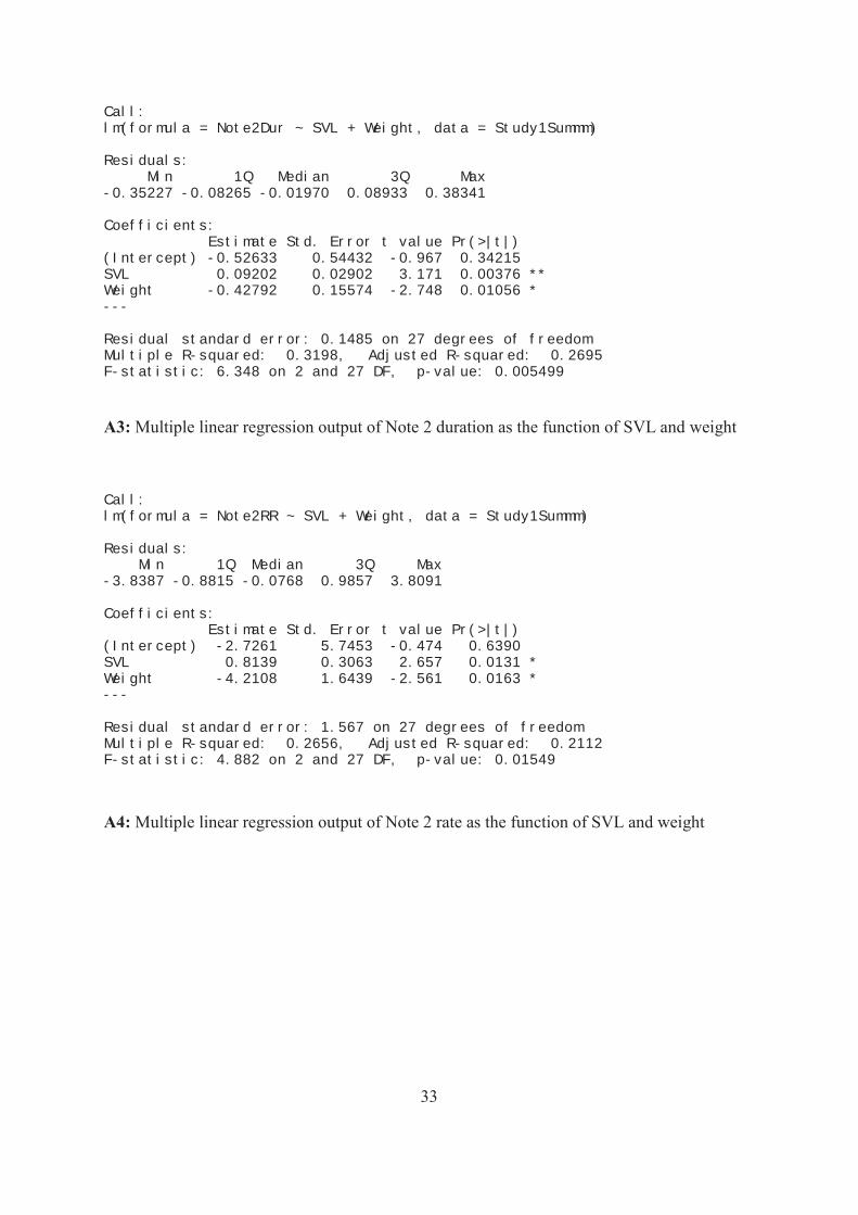
Call: lm(formula = Note2Dur ~ SVL + Weight, data = Study1Summm) Residuals: Min 1Q Median 3Q Max -0.35227 -0.08265 -0.01970 0.08933 0.38341 Coefficients: Estimate Std. Error t value Pr(>|t|) (Intercept) -0.52633 0.54432 -0.967 0.34215 SVL 0.09202 0.02902 3.171 0.00376 ** Weight -0.42792 0.15574 -2.748 0.01056 * --- Residual standard error: 0.1485 on 27 degrees of freedom Multiple R-squared: 0.3198, Adjusted R-squared: 0.2695 F-statistic: 6.348 on 2 and 27 DF, p-value: 0.005499
A3: Multiple linear regression output of Note 2 duration as the function of SVL and weight
Call: lm(formula = Note2RR ~ SVL + Weight, data = Study1Summm) Residuals: Min 1Q Median 3Q Max -3.8387 -0.8815 -0.0768 0.9857 3.8091 Coefficients: Estimate Std. Error t value Pr(>|t|) (Intercept) -2.7261 5.7453 -0.474 0.6390 SVL 0.8139 0.3063 2.657 0.0131 * Weight -4.2108 1.6439 -2.561 0.0163 * --- Residual standard error: 1.567 on 27 degrees of freedom Multiple R-squared: 0.2656, Adjusted R-squared: 0.2112 F-statistic: 4.882 on 2 and 27 DF, p-value: 0.01549
A4: Multiple linear regression output of Note 2 rate as the function of SVL and weight

34
Call: lm(formula = CallRate ~ Weight, data = Study1Summm) Residuals: Min 1Q Median 3Q Max -3.1596 -1.2513 0.1124 0.6853 5.8966 Coefficients: Estimate Std. Error t value Pr(>|t|) (Intercept) 12.766 2.912 4.384 0.000149 *** Weight -5.969 1.943 -3.073 0.004690 ** --- Residual standard error: 2.016 on 28 degrees of freedom Multiple R-squared: 0.2522, Adjusted R-squared: 0.2254 F-statistic: 9.441 on 1 and 28 DF, p-value: 0.00469
A5: Multiple linear regression output of call rate as the function of body weight
Call: lm(formula = AvgSilInt ~ Weight, data = Study1Summm) Residuals: Min 1Q Median 3Q Max -11.8257 -3.9498 -0.5762 4.1195 10.3936 Coefficients: Estimate Std. Error t value Pr(>|t|) (Intercept) -11.34 8.02 -1.414 0.16849 Weight 15.61 5.35 2.917 0.00689 ** --- Residual standard error: 5.553 on 28 degrees of freedom Multiple R-squared: 0.2331, Adjusted R-squared: 0.2057 F-statistic: 8.509 on 1 and 28 DF, p-value: 0.006889
A6: Multiple linear regression output of silent interval as the function of body weight

35