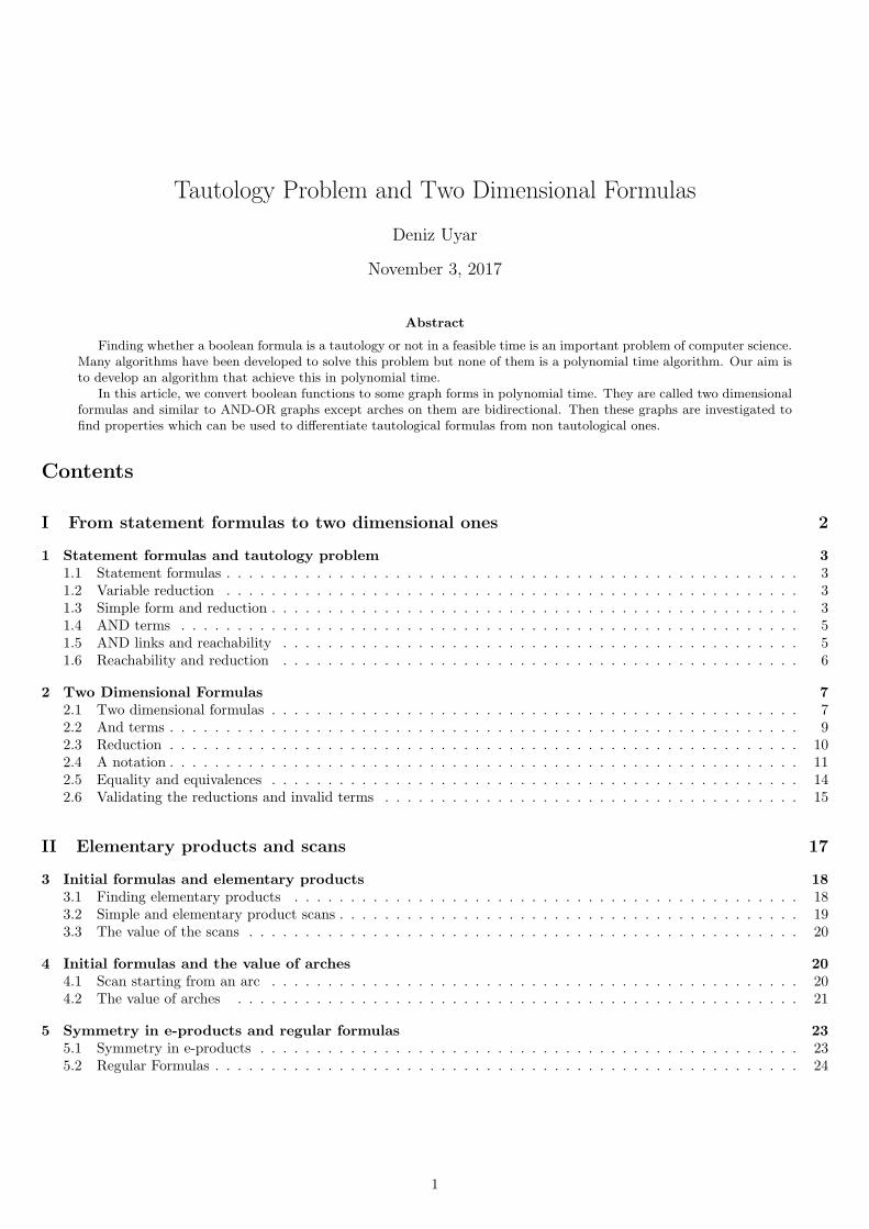
Tautology Problem and Two Dimensional Formulas

Deniz Uyar

November 3, 2017

Abstract

Finding whether a boolean formula is a tautology or not in a feasible time is an important problem of computer science.Many algorithms have been developed to solve this problem but none of them is a polynomial time algorithm. Our aim isto develop an algorithm that achieve this in polynomial time.

In this article, we convert boolean functions to some graph forms in polynomial time. They are called two dimensionalformulas and similar to AND-OR graphs except arches on them are bidirectional. Then these graphs are investigated tofind properties which can be used to differentiate tautological formulas from non tautological ones.

Contents

I From statement formulas to two dimensional ones 2

1 Statement formulas and tautology problem 31.1 Statement formulas . . . . . . . . . . . . . . . . . . . . . . . . . . . . . . . . . . . . . . . . . . . . . . . . . . . 31.2 Variable reduction . . . . . . . . . . . . . . . . . . . . . . . . . . . . . . . . . . . . . . . . . . . . . . . . . . . 31.3 Simple form and reduction . . . . . . . . . . . . . . . . . . . . . . . . . . . . . . . . . . . . . . . . . . . . . . . 31.4 AND terms . . . . . . . . . . . . . . . . . . . . . . . . . . . . . . . . . . . . . . . . . . . . . . . . . . . . . . . 51.5 AND links and reachability . . . . . . . . . . . . . . . . . . . . . . . . . . . . . . . . . . . . . . . . . . . . . . 51.6 Reachability and reduction . . . . . . . . . . . . . . . . . . . . . . . . . . . . . . . . . . . . . . . . . . . . . . 6

2 Two Dimensional Formulas 72.1 Two dimensional formulas . . . . . . . . . . . . . . . . . . . . . . . . . . . . . . . . . . . . . . . . . . . . . . . 72.2 And terms . . . . . . . . . . . . . . . . . . . . . . . . . . . . . . . . . . . . . . . . . . . . . . . . . . . . . . . . 92.3 Reduction . . . . . . . . . . . . . . . . . . . . . . . . . . . . . . . . . . . . . . . . . . . . . . . . . . . . . . . . 102.4 A notation . . . . . . . . . . . . . . . . . . . . . . . . . . . . . . . . . . . . . . . . . . . . . . . . . . . . . . . . 112.5 Equality and equivalences . . . . . . . . . . . . . . . . . . . . . . . . . . . . . . . . . . . . . . . . . . . . . . . 142.6 Validating the reductions and invalid terms . . . . . . . . . . . . . . . . . . . . . . . . . . . . . . . . . . . . . 15

II Elementary products and scans 17

3 Initial formulas and elementary products 183.1 Finding elementary products . . . . . . . . . . . . . . . . . . . . . . . . . . . . . . . . . . . . . . . . . . . . . 183.2 Simple and elementary product scans . . . . . . . . . . . . . . . . . . . . . . . . . . . . . . . . . . . . . . . . . 193.3 The value of the scans . . . . . . . . . . . . . . . . . . . . . . . . . . . . . . . . . . . . . . . . . . . . . . . . . 20

4 Initial formulas and the value of arches 204.1 Scan starting from an arc . . . . . . . . . . . . . . . . . . . . . . . . . . . . . . . . . . . . . . . . . . . . . . . 204.2 The value of arches . . . . . . . . . . . . . . . . . . . . . . . . . . . . . . . . . . . . . . . . . . . . . . . . . . 21

5 Symmetry in e-products and regular formulas 235.1 Symmetry in e-products . . . . . . . . . . . . . . . . . . . . . . . . . . . . . . . . . . . . . . . . . . . . . . . . 235.2 Regular Formulas . . . . . . . . . . . . . . . . . . . . . . . . . . . . . . . . . . . . . . . . . . . . . . . . . . . . 24

1

6 Reduced formulas and e-product scanning 266.1 Validity of e-product scanning algorithm . . . . . . . . . . . . . . . . . . . . . . . . . . . . . . . . . . . . . . . 266.2 An example . . . . . . . . . . . . . . . . . . . . . . . . . . . . . . . . . . . . . . . . . . . . . . . . . . . . . . . 276.3 Paths . . . . . . . . . . . . . . . . . . . . . . . . . . . . . . . . . . . . . . . . . . . . . . . . . . . . . . . . . . 276.4 Paths and E-scans . . . . . . . . . . . . . . . . . . . . . . . . . . . . . . . . . . . . . . . . . . . . . . . . . . . 286.5 Values of the arches . . . . . . . . . . . . . . . . . . . . . . . . . . . . . . . . . . . . . . . . . . . . . . . . . . 29

7 Elementary sums 297.1 E-sum scans . . . . . . . . . . . . . . . . . . . . . . . . . . . . . . . . . . . . . . . . . . . . . . . . . . . . . . . 297.2 Simple and elementary sums . . . . . . . . . . . . . . . . . . . . . . . . . . . . . . . . . . . . . . . . . . . . . . 307.3 e-product scans vs e-sum scans . . . . . . . . . . . . . . . . . . . . . . . . . . . . . . . . . . . . . . . . . . . . 31

III Tautological properties 33

8 Tautological properties in last reduced forms 348.1 The values of the infinite paths . . . . . . . . . . . . . . . . . . . . . . . . . . . . . . . . . . . . . . . . . . . . 348.2 A demonstration . . . . . . . . . . . . . . . . . . . . . . . . . . . . . . . . . . . . . . . . . . . . . . . . . . . . 35

9 Further studies 37

Part I

From statement formulas to two dimensional ones

2

1 Statement formulas and tautology problem

1.1 Statement formulas

Boolean functions( or any functions in general) can be represented in various ways. In this section, we consider only theboolean functions given as a string consist of AND, OR, NOT signs, variable signs, constants 0 and 1 and parenthesis writtenas usual. We will use ·(point), ∧ and˜for the AND, OR, NOT signs and use the letters similar to x,y,z alone or with indicesto represent variables.

Suppose the variables in a statement formula be (x1, .., xn). If we assign either 0 or 1 value to each of the variables,then we get an interpretation of these variables. For example (0, 0, 0) is an interpretation of the variables (x1, x2, x3). Letrepresent a function as f(x1, .., xn). If (x1, x2, x3) is the list of the variables in a function, then the value of the functionf(x1, x2, x3) becomes f(0, 0, 0) for the interpretation (0, 0, 0). If two functions have the same variables and gives the sameresults for every interpretation of their variables, then these are equal functions. Otherwise they are different functions. Forexample the functions f1(x, y) = x · y and f2(x, y) = x ∨ y are different because f1(0, 1) = 0 and f2(0, 1) = 1 true for theinterpretation (0, 1). The number of different functions for the n variables would be 22

n

.A boolean function is said a tautology if it gives the value 1 for every interpretation of its variables. For example 1 or

x ∨ x gives 1 for all the interpretation of a variable list. Therefore 1 and x ∨ x functions are tautologies.There are infinite number of different formulas representing the same function. For example x∨y is equal to x∨y∨x∨y..x∨y

where x ∨ y is duplicated as many times as desired. Then, the tautology checking problem may be expressed as ”is a givenformula a different writing of the function 1”.

The most straightforward way of checking whether a formula is tautology or not is to evaluate the formula for eachinterpretations of the variables. The number of interpretation for n different variables is 2n. The number of differentvariables in a formula is at most s/2 where s is the length of the formula. So the function must be evaluated 2s/2 times.That is the complexity is O(s2s/2). This is not polynomial. So we will investigate various ways to achieve this in polynomialtime.

1.2 Variable reduction

Proposition 1 f(x1, .., xi, .., xn) is a tautology if and only if f(x1, .., 0, .., xn) · f(x1, .., 1, .., xn) is a tautology.

Proof 1 Trivial.

According to this proposition, from a formula, we can obtain another one which has one less variable and still preservesthe tautological property of the original one. This is a variable reduction operation and can be illustrated as

f(x1, .., xi, .., xn)xi→ f(x1, .., 0, .., xn) · f(x1..1..xn)

Let call this v-reduction.All the variables of a boolean formula can be eliminated by a series of v-reductions. After simplification, what would be

in hand at last, is either a 1 or 0. Since each v-reduction preserves the tautological property of the original formula, a 1 athand means the original formula is a tautology an 0 means it is not a tautology.

The obvious way of doing reduction is to get two formulas r1 and r2 as follows; replace xi with 0 in the initial formulato obtain r1 and replace xi with 1 in the initial formula to obtain r2, parenthesise them if necessary and put an AND signbetween them. Also all the 1’s and 0’s are removed from the formula by applying the identities

0 · x = 0, 1 · x = x, 0 · x = x, 1 · x = 1, 0 = 1, 1 = 0.All of these process takes polynomial time. However the length of (r1) · (r2) which is the resulting formula would be 2s

approximately in the worst case. Doing this for s/2 variables would give us a complexity of O(s · 2s/2, so it seems that thisprocess could not be achieved in polynomial time.

1.3 Simple form and reduction

A variable, the inverse of a variable and the constants 0,1 are called atomic terms.If a formula is in the form a1 ∨ a2 ∨ .. ∨ an then it is a disjunction. Each ai is an element of it. If all the elements of a

disjunction is an atomic term then this is a simple sum. For example x1 ∨ x1 is a simple sum.If a formula is in the form a1 · a2 · .. · an then it is a conjunction. Each ai is an element of it. If all the elements of a

conjunction is an atomic term then this is a simple product. For example x1 · x1 is a simple product.If all the elements of a disjunction are simple products, then the formula is said to be in the disjunctive normal form.

Each boolean formula has a disjunctive normal form or DNF. In this form, each element of the form is called an elementaryproduct or e-product and either contain xi or xi or neither contain xi nor xi as follows.

xi · α1 ∨ .. ∨ xi · αn ∨ xi · β1 ∨ .. ∨ xi · βm ∨ δ1 ∨ .. ∨ δlHere δk is the elementary product including neither xi nor xi. The elementary products which include both xi and xi

are either xi · αi or xi.βj .

3

This formula can be written simply as

xi · α ∨ xi · β ∨ δ

where α = α1 ∨ .. ∨ αn, β = β1 ∨ .. ∨ βm ve δ = δ1 ∨ .. ∨ δlIf α includes xi and/or xi, then they can be eliminated by the following equivalences.

xi · α(xi) = xi · α(1)xi · α(xi) = xi · α(0)

Similarly if any βj includes xi or xi, they are eliminated by

xi · β(xi) = xi · β(0)xi · β(xi) = xi · β(1)

Thus, the terms α, β, δ do not include xi or xi. This is called as ”simple form”. Now let see the reduction in this form.

xi · α ∨ xi · β ∨ δxi→ (β ∨ δ) · (α ∨ δ)

= β · α ∨ δ

After this point on, we will assume the NOT operator is applied to the variable symbols only. If a formula is not in thisform, then an equivalent formula in this form can be obtained in polynomial time.[2]

The DNF form of a given formula can be produced by applying the rule x · (y∨ z) = x ·y∨x · z to the formula recursively.Then the right hand side of the v-reduction could be obtained by examining each elementary product to mark them as αi,βj

or δk and by doing the necessary operations to get α · β ∨ δ. However, the number of elementary products is not polynomialwrt n which is the number of different variables. Therefore, obtaining all the elementary products in this way dos not takepolynomial time.

So let investigate the other ways of reducing the formula. It can easily be seen that, if a formula does not have xi butincludes xi, then the simple form would be xi · β ∨ δ and the reduction becomes as

xi · β ∨ δxi→ (β ∨ δ) · δ

= δ

But this can be achieved simply by putting 0 instead of xi and eliminating 0’s from the formula.

xi · β ∨ δxi→ 0 · β ∨ δ = δ

⇒ f(xi)xi→ f(0)

This process can be applied to the original formula in polynomial time. Similarly for the formulas which does not includexi but having xi, reducing is achieved as

xi · α ∨ δxi→ (α ∨ δ) · δ = δ

⇒ f(xi)xi→ f(0)

Again the reduced form can be obtained from the original one by replacing xi with 0 and eliminating all 0sThus any variable which occurs either only alone or only with negation can be eliminated by just replacing them with 0.

This takes polynomial time. As a result, a formula is obtained in which all the variables occur at least twice; one as aloneand the other with negation. Now if we evaluate the formula by examining every interpretations of them, the complexitywould be O(s.2s/2) since the number of different variables is s/4 at most in such a formula.

In the rest of this section we will assume all the variables are not alone. If they are not in this form, they can be changedto this form in polynomial time as mentioned above.

4

1.4 AND terms

Consider the v-reduction again.f(xi, xi) = xi · α ∨ xi.β ∨ δ

xi→ β · α ∨ δHere the question is that ”are there alternate ways of obtaining the right hand side of the reduction from the left hand

side”.The answer is yes and as shown below, the formula can be reduced by replacing xi with βi and xi with 0.

xi · α ∨ xi.β ∨ δxi→ xi/

β

· α ∨ xi/0.β ∨ δ

= β · α ∨ δ

The same result can be obtained by replacing xi with 0 and xi with α,

xi · α ∨ xi.β ∨ δxi→ xi/

0· α ∨ xi/

α.β ∨ δ

= β · α ∨ δ

or by replacing xi with β and xi with α.

xi · α ∨ xi.β ∨ δxi→ xi/

β

· α ∨ xi/α.β ∨ δ

= β · α ∨ δ

α and β are just the terms conjuncted with xi and xi respectively. So, this idea can be applied to any formula even it isnot in DNF form.

f(xi, xi)xi→ f(β, 0)

f(xi, xi)xi→ f(0, α)

f(xi, xi)xi→ f(β, α)

Definition 1 If two terms t1 and t2 are conjuncted then t2 is an A-term of t1 and vice versa

For example in (x ∨ y) · z, (x ∨ y) is an A-term of z and z is an A-term of (x ∨ y).Then the idea ”replace xi with β” becomes ”replace each occurrence of xi with the A-term of xi”. Similarly, the idea

”replace xi with α” becomes ”replace each occurrence of xi with the A-term of xi”

1.5 AND links and reachability

Let try to find the and-terms of xi without changing the formula.In any formula, each occurrence of xi in a formula is in the following form...lm · (uk ∨ .. ∨ l2 · (ui ∨ l1 · xi · r1 ∨ ui−1) · r2 ∨ .. ∨ u1) · rn ∨ ..The term which is directly conjuncted with xi is l1 · r1. If the parenthesis are opened then the A-term of xi for this

occurrence would be lm..l2 · l1 · r1 · r2..rn. Let this be αk where k represents the k’th occurrence of xi. If αk contains xi

or xi, then they can be eliminated by replacing them with 1 and 0 respectively, since αk is an A-term of xi . That is theequivalences α(xi) = α(1) and α(xi) = α(0) are applied. The entire A-term of xi then becomes α = α1 ∨ .. ∨ αn where n isthe number of occurrences of xi in the formula.

One algorithm to do this is the following.

Algorithm 1 Find an occurrence of xi. Do the followings for this occurrence.

1. Let T be an empty set and xi is the last A-term.

5

2. Do the following steps toward right until the end of the formula

(a) If t1 is the last A-term and the formula is in the form ..t1 · t2.. then make t2 the last A-term and put it into T.

(b) If the formula is in the form ..(.. ∨ t · ti ∨ .. ∨ tn) · r.. and ti is the last A-term, then make r the last A-term andput it into T.

3. Starting from xi, do the following steps toward left until the end of the formula.

(a) If t2 is the last A-term and the formula is in the form ..t1 · t2.. then make t1 the last A-term and put it into T.

(b) f t is the last A-term and the formula is in the form ..l · (t1 ∨ .. ∨ t · ti ∨ .. ∨ tn).., then make l is the last A-termand put it into T.

The A-term of the this occurrence would be a1 · .. · an where ai ∈ T

In this case, the A-term of xi, i.e. α, is the disjunction of the A-terms of all the occurrences of xi. If the number ofoccurrences of xi is n and the length of the formula is s, this operation takes ns times. If there are xi or xi terms in α, thenthey are eliminated by the equations α(xi, xi) = α(1, 0). β is found similarly. The term δ can be found by replacing xi andxi with 0. All of these jobs take polynomial time. So the reduced formula α ·β∨δ can be found in polynomial time. However,the length of the formula found may be larger than the original one. If the length of the formula found is 2s in average thenthe length seems to increase exponential in each reduction. On the other hand, the number of different variables would bereduced by one and thus the length can not increase so much. From here, one may prove that the length can not increaseexponentially. However, we will assume that this process can not be realized in polynomial time.

The algorithm above replaces the concept of finding an A-term with the concept of going from one term to another. Tovisualise this concept, we will use − symbol instead of ·. By this notation, a statement formula would look like

..lm − (uk ∨ .. ∨ l2 − (ui ∨ l1 − xi − r1 ∨ ui−1)− r2 ∨ .. ∨ u1)− rn ∨ ..Thus − represents both reachability and A-links. So, two terms are conjuncted to each other if they are reachable to

each other by the following rules.

1. In t1 − t2, from t1 one can reach to t2 and vice versa.

2. In (t1 ∨ t2)− t3, t3 is reached from t1 or from t2 and from t3, t1 or t2 can be reached.

3. If t2 is reachable from t1 and t3 is reachable from t2, then t3 is reachable from t1.

So, if t2 is reachable from t1 then t2 is an A-term of t1.

1.6 Reachability and reduction

Now consider the v-reduction again.

xi − α ∨ xi − β ∨ δxi→ (β ∨ δ)− (α ∨ δ)

= β − α ∨ δ

Note that after replacement α becomes conjuncted to β and vice versa. To make two term conjuncted, it is sufficient tomade them reachable from each other. So the idea can be realized by putting an A-link between α and β as shown below.

| |xi − α ∨ xi − β ∨ δ

xi→ 1− α ∨ 1− β ∨ δ

This path make α and β reachable to each other and thus they become A-terms of each other. A better realization ofthis is as follows

| |xi − α ∨ xi − β ∨ δ

xi→ 1− α ∨ 1− β ∨ δ

α and β become A-term of each other via 1’s linked to them.

6

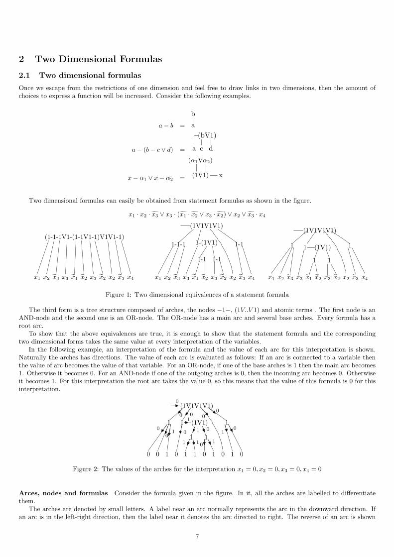
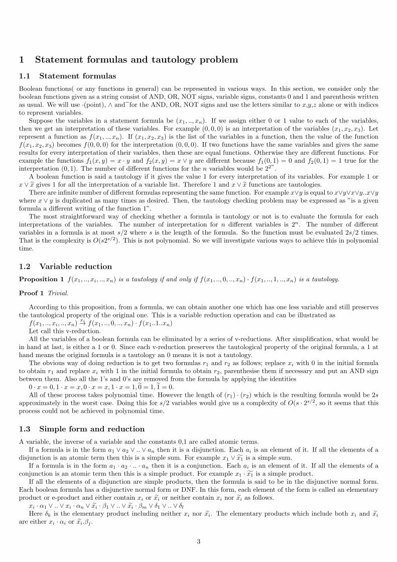
2 Two Dimensional Formulas

2.1 Two dimensional formulas

Once we escape from the restrictions of one dimension and feel free to draw links in two dimensions, then the amount ofchoices to express a function will be increased. Consider the following examples.

a− b =

b

a

a− (b− c ∨ d) =

(bV1)

ca d

x− α1 ∨ x− α2 = x(1V1)

(α1Vα2)

Two dimensional formulas can easily be obtained from statement formulas as shown in the figure.

x1 · x2 · x3 ∨ x3 · (x1 · x2 ∨ x3 · x2) ∨ x2 ∨ x3 · x4

x1 x2 x3 x3 x2 x4x3 x1 x2 x2 x3

(1-1-1V1-(1-1V1-1)V1V1-1)

x1 x2 x3 x3 x2 x4x3 x1 x2 x2 x3

1-11-1

1-1-1 1-1

(1V1V1V1)

1-(1V1)

x1 x2 x3 x3 x2 x4x3 x1 x2 x2 x3

1

11

1(1V1)

(1V1V1V1)

1

Figure 1: Two dimensional equivalences of a statement formula

The third form is a tree structure composed of arches, the nodes −1−, (1V..V 1) and atomic terms . The first node is anAND-node and the second one is an OR-node. The OR-node has a main arc and several base arches. Every formula has aroot arc.

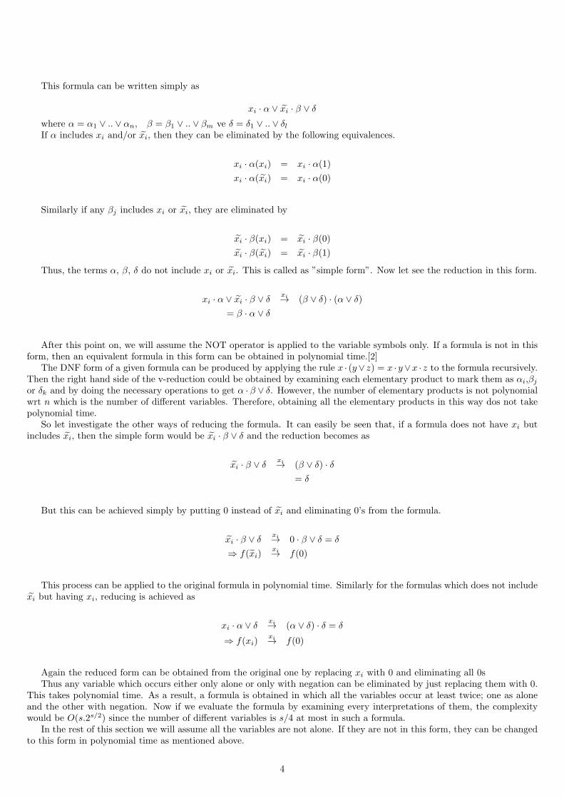
To show that the above equivalences are true, it is enough to show that the statement formula and the correspondingtwo dimensional forms takes the same value at every interpretation of the variables.

In the following example, an interpretation of the formula and the value of each arc for this interpretation is shown.Naturally the arches has directions. The value of each arc is evaluated as follows: If an arc is connected to a variable thenthe value of arc becomes the value of that variable. For an OR-node, if one of the base arches is 1 then the main arc becomes1. Otherwise it becomes 0. For an AND-node if one of the outgoing arches is 0, then the incoming arc becomes 0. Otherwiseit becomes 1. For this interpretation the root arc takes the value 0, so this means that the value of this formula is 0 for thisinterpretation.

1

11

1(1V1)1

(1V1V1V1)

0 0 1 0 1 1 0 1 0 1 0

0

01 0

1 1

1

01

0

100

0

00

10

Figure 2: The values of the arches for the interpretation x1 = 0, x2 = 0, x3 = 0, x4 = 0

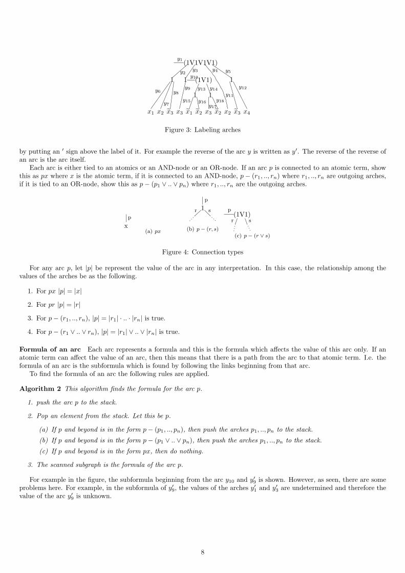
Arces, nodes and formulas Consider the formula given in the figure. In it, all the arches are labelled to differentiatethem.

The arches are denoted by small letters. A label near an arc normally represents the arc in the downward direction. Ifan arc is in the left-right direction, then the label near it denotes the arc directed to right. The reverse of an arc is shown

7

x1 x2 x3 x3 x2 x4x3 x1 x2 x2 x3

1

11

1(1V1)1

(1V1V1V1)y1

y2y3 y4 y5

y6

y7

y8y9

y10

y12y13 y14

y15 y16y17

y18y11

Figure 3: Labeling arches

by putting an ′ sign above the label of it. For example the reverse of the arc y is written as y′. The reverse of the reverse ofan arc is the arc itself.

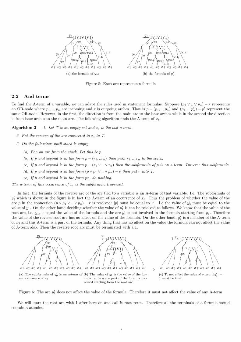
Each arc is either tied to an atomics or an AND-node or an OR-node. If an arc p is connected to an atomic term, showthis as px where x is the atomic term, if it is connected to an AND-node, p− (r1, .., rn) where r1, .., rn are outgoing arches,if it is tied to an OR-node, show this as p− (p1 ∨ .. ∨ pn) where r1, .., rn are the outgoing arches.

x

p

(a) px

r s

p

1

(b) p− (r, s)

r s(1V1)

p

(c) p− (r ∨ s)

Figure 4: Connection types

For any arc p, let |p| be represent the value of the arc in any interpretation. In this case, the relationship among thevalues of the arches be as the following.

1. For px |p| = |x|

2. For pr |p| = |r|

3. For p− (r1, .., rn), |p| = |r1| · .. · |rn| is true.

4. For p− (r1 ∨ .. ∨ rn), |p| = |r1| ∨ .. ∨ |rn| is true.

Formula of an arc Each arc represents a formula and this is the formula which affects the value of this arc only. If anatomic term can affect the value of an arc, then this means that there is a path from the arc to that atomic term. I.e. theformula of an arc is the subformula which is found by following the links beginning from that arc.

To find the formula of an arc the following rules are applied.

Algorithm 2 This algorithm finds the formula for the arc p.

1. push the arc p to the stack.

2. Pop an element from the stack. Let this be p.

(a) If p and beyond is in the form p− (p1, .., pn), then push the arches p1, .., pn to the stack.

(b) If p and beyond is in the form p− (p1 ∨ .. ∨ pn), then push the arches p1, .., pn to the stack.

(c) If p and beyond is in the form px, then do nothing.

3. The scanned subgraph is the formula of the arc p.

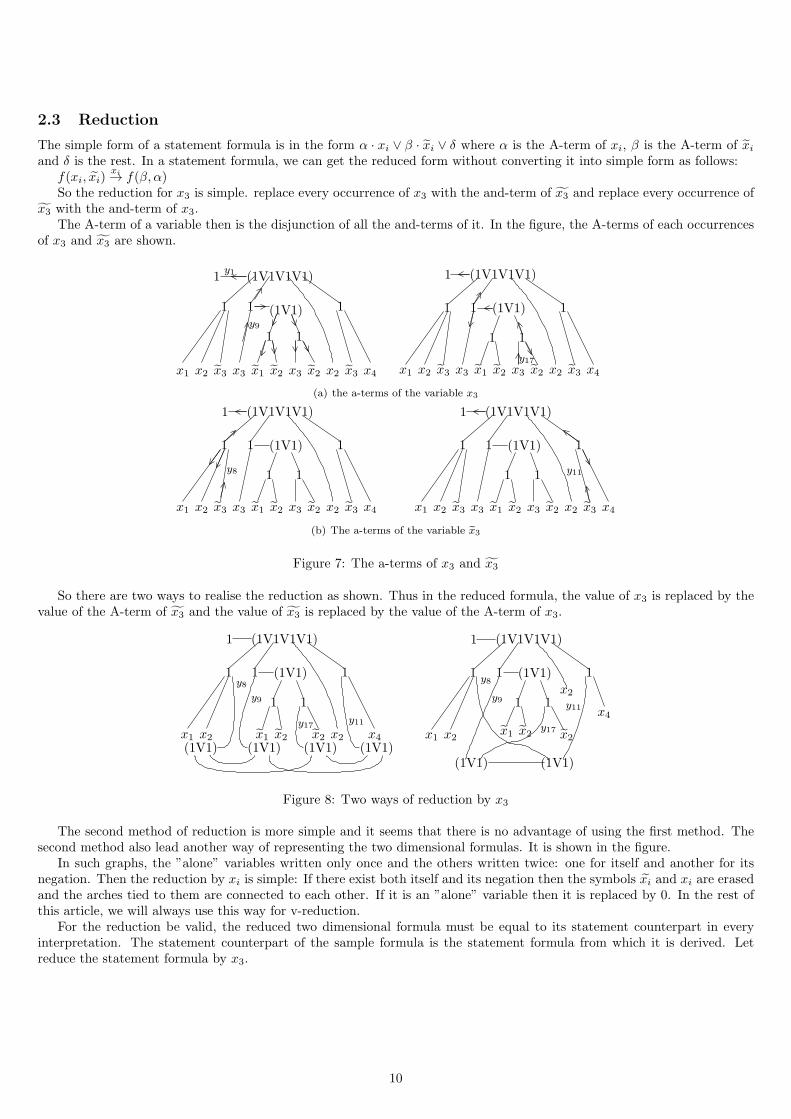
For example in the figure, the subformula beginning from the arc y10 and y′9 is shown. However, as seen, there are someproblems here. For example, in the subformula of y′9, the values of the arches y′1 and y′3 are undetermined and therefore thevalue of the arc y′9 is unknown.

8

x1 x2 x3 x3 x2 x4x3 x1 x2 x2 x3

1

11

1(1V1)1

(1V1V1V1)y1

y2y3 y4 y5

y6

y7

y8y9

y10

y12y13 y14

y15 y16y17

y18y11

(a) the formula of y10

x1 x2 x3 x3 x2 x4x3 x1 x2 x2 x3

1

11

1(1V1)1

(1V1V1V1)y1

y2y3 y4 y5

y6

y7

y8y9

y10

y12y13 y14

y15 y16y17

y18y11

(b) the formula of y′9

Figure 5: Each arc represents a formula

2.2 And terms

To find the A-term of a variable, we can adapt the rules used in statement formulas. Suppose (p1 ∨ .. ∨ pn) − r representsan OR-node where p1, .., pn are incoming and r is outgoing arches. That is p − (p1, .., pn) and (p′1, .., p

′n) − p′ represent the

same OR-node. However, in the first, the direction is from the main arc to the base arches while in the second the directionis from base arches to the main arc. The following algorithm finds the A-term of xi.

Algorithm 3 1. Let T is an empty set and xi is the last a-term.

2. Put the reverse of the arc connected to xi to T.

3. Do the followings until stack is empty.

(a) Pop an arc from the stack. Let this be p.

(b) If p and beyond is in the form p− (r1, ..rn) then push r1, .., rn to the stack.

(c) If p and beyond is in the form p− (r1 ∨ .. ∨ rn) then the subformula of p is an a-term. Traverse this subformula.

(d) If p and beyond is in the form (p ∨ p1 ∨ .. ∨ pn)− r then put r into T.

(e) If p and beyond is in the form px, do nothing.

The a-term of this occurrence of xi is the subformula traversed.

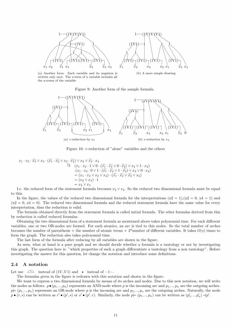
In fact, the formula of the reverse arc of the arc tied to a variable is an A-term of that variable. I.e. The subformula ofy′9 which is shown in the figure is in fact the A-term of an occurrence of x3. Thus the problem of whether the value of thearc p in the connection (p ∨ p1 ∨ .. ∨ pn) − r is resolved: |p| must be equal to |r|. I.e the value of y′3 must be equal to thevalue of y′1. On the other hand deciding whether the value of y′1 is can be resolved as follows. We know that the value of theroot arc, i.e. y1, is equal the value of the formula and the arc y′1 is not involved in the formula starting from y1. Thereforethe value of the reverse root arc has no affect on the value of the formula. On the other hand, y′1 is a member of the A-termof x3 and this A-term is a part of the formula. Any thing that has no affect on the value the formula can not affect the valueof A-term also. Then the reverse root arc must be terminated with a 1.

x1 x2 x3 x3 x2 x4x3 x1 x2 x2 x3

1

11

1(1V1)1

(1V1V1V1)

y9

y1

y3y10

(a) The subformula of y′9 is an a-term ofan occurrence of x3

x1 x2 x3 x3 x2 x4x3 x1 x2 x2 x3

1

11

1(1V1)

(1V1V1V1)

y9

y1

y3y10

1

(b) The value of y1 is the value of the for-mula. y′1 is not a part of the formula tra-versed starting from the root arc

⇒

1

11

1(1V1)1

(1V1V1V1)

y9

x1 x2 x3 x3 x2 x4x3 x1 x2 x2 x3

y11

(c) To not affect the value of a-term, |y′1| =1 must be true

Figure 6: The arc y′1 does not affect the value of the formula. Therefore it must not affect the value of any A-term

We will start the root arc with 1 after here on and call it root term. Therefore all the terminals of a formula wouldcontain a atomics.

9

2.3 Reduction

The simple form of a statement formula is in the form α · xi ∨ β · xi ∨ δ where α is the A-term of xi, β is the A-term of xi

and δ is the rest. In a statement formula, we can get the reduced form without converting it into simple form as follows:f(xi, xi)

xi→ f(β, α)So the reduction for x3 is simple. replace every occurrence of x3 with the and-term of x3 and replace every occurrence of

x3 with the and-term of x3.The A-term of a variable then is the disjunction of all the and-terms of it. In the figure, the A-terms of each occurrences

of x3 and x3 are shown.

1

11

1(1V1)1

(1V1V1V1)

y9

x1 x2 x3 x3 x2 x4x3 x1 x2 x2 x3

y11

x1 x2 x3 x3 x2 x4x3 x1 x2 x2 x3

1

11

1(1V1)1

(1V1V1V1)

y17

1

(a) the a-terms of the variable x3

1

11

1(1V1)1

(1V1V1V1)

y8

1

x1 x2 x3 x3 x2 x4x3 x1 x2 x2 x3

1

11

1(1V1)1

(1V1V1V1)1

x1 x2 x3 x3 x2 x4x3 x1 x2 x2 x3

y11

(b) The a-terms of the variable x3

Figure 7: The a-terms of x3 and x3

So there are two ways to realise the reduction as shown. Thus in the reduced formula, the value of x3 is replaced by thevalue of the A-term of x3 and the value of x3 is replaced by the value of the A-term of x3.

1

11

1(1V1)1

(1V1V1V1)1

x1 x2 x2 x4x1 x2 x2

(1V1) (1V1) (1V1)(1V1)

y8

y9

y11y17

1

11

1(1V1)1

(1V1V1V1)1

x1 x2 x2

x2

x4

x1 x2

(1V1)(1V1)

y8

y9y11

y17

Figure 8: Two ways of reduction by x3

The second method of reduction is more simple and it seems that there is no advantage of using the first method. Thesecond method also lead another way of representing the two dimensional formulas. It is shown in the figure.

In such graphs, the ”alone” variables written only once and the others written twice: one for itself and another for itsnegation. Then the reduction by xi is simple: If there exist both itself and its negation then the symbols xi and xi are erasedand the arches tied to them are connected to each other. If it is an ”alone” variable then it is replaced by 0. In the rest ofthis article, we will always use this way for v-reduction.

For the reduction be valid, the reduced two dimensional formula must be equal to its statement counterpart in everyinterpretation. The statement counterpart of the sample formula is the statement formula from which it is derived. Letreduce the statement formula by x3.

10

1

1

(1V1V1V1)1

(1V1)

1 (1V1)1

(1V1)

1

x2x1 x1 x3

(1V1) (1V1)

x4x3x2

(a) Another form. Each variable and its negation iswritten only once. The a-term of a variable includes allthe a-terms of the variable

1

(1V1V1V1)1

(1V1)

x4x3x3

(1V1)(1V1)

x2

1(1V1)

1

x1

(1V1)

x2 x1

1

1

(b) A more simple drawing

Figure 9: Another form of the sample formula.

1

(1V1V1V1)1

(1V1)

x411

(1V1)(1V1)

x2

1(1V1)

1

x1

(1V1)

x2 x1

1

1

(a) v-reduction by x3

1

(1V1V1V1)1

(1V1)

0x3x3

(1V1)(1V1)

x2

1(1V1)

1

x1

(1V1)

x2 x1

1

1

(b) v-reduction by x4

Figure 10: v-reduction of ”alone” variables and the others

x1 · x2 · x3 ∨ x3 · (x1 · x2 ∨ x3 · x2) ∨ x2 ∨ x3 · x4x3→ (x1 · x2 · 1 ∨ 0 · (x1 · x2 ∨ 0 · x2) ∨ x2 ∨ 1 · x4)

·(x1 · x2 · 0 ∨ 1 · (x1 · x2 ∨ 1 · x2) ∨ x2 ∨ 0 · x4)= (x1 · x2 ∨ x2 ∨ x4) · (x1 · x2 ∨ x2 ∨ x2)= (x2 ∨ x4) · 1= x2 ∨ x4

I.e. the reduced form of the statement formula becomes x2 ∨ x4. So the reduced two dimensional formula must be equalto this.

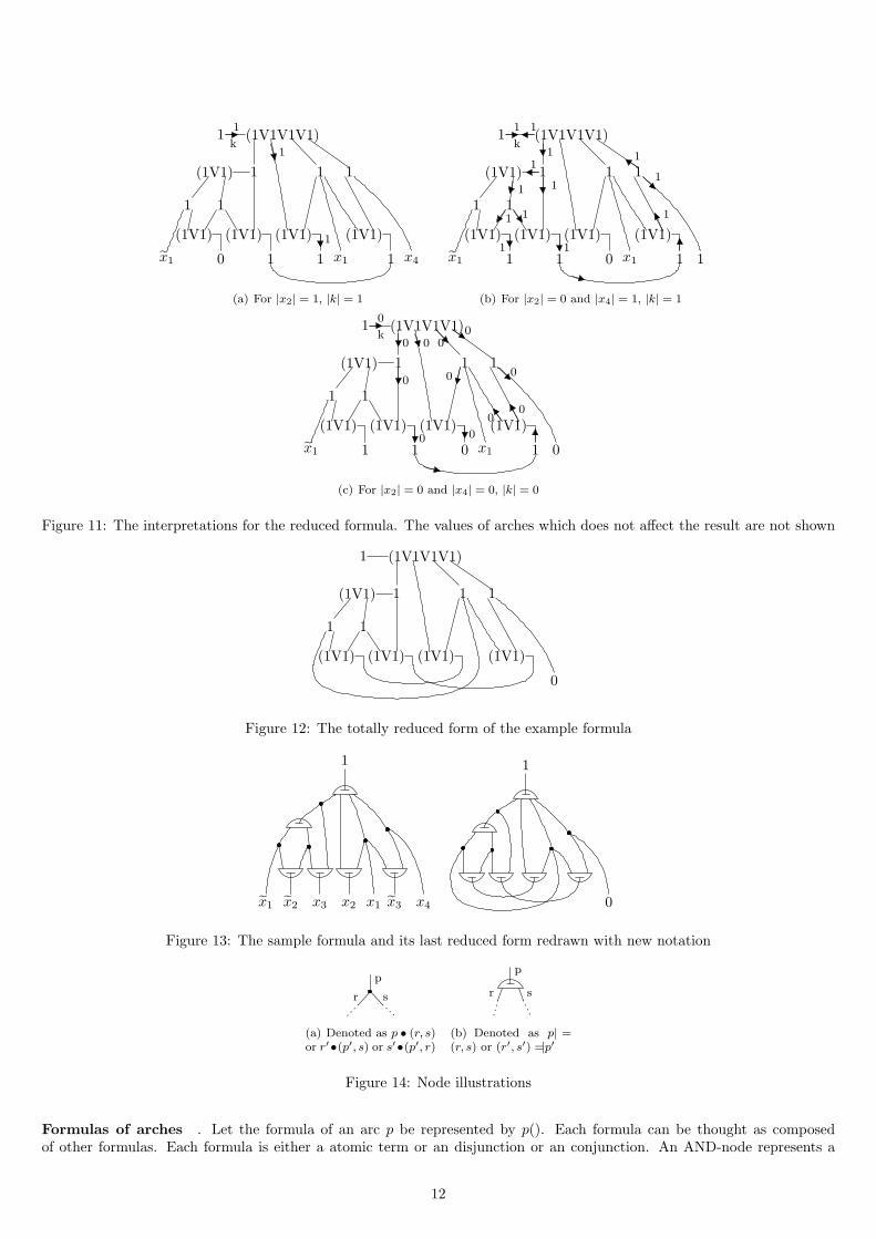
In the figure, the values of the reduced two dimensional formula for the interpretations (x2 = 1),(x2 = 0, x4 = 1) and(x2 = 0, x4 = 0). The reduced two dimensional formula and the reduced statement formula have the same value for everyinterpretation, thus the reduction is valid.

The formula obtained directly from the statement formula is called initial formula. The other formulas derived from thisby reduction is called reduced formulas.

Obtaining the two dimensional form of a statement formula as mentioned above takes polynomial time. For each differentvariables, one or two OR-nodes are formed. For each atomics, an arc is tied to this nodes. So the total number of archesbecomes the number of parenthesis + the number of atomic terms + 2*number of different variables. It takes O(s) times toform the graph. The reduction also takes polynomial time.

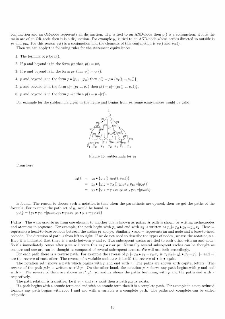
The last form of the formula after reducing by all variables are shown in the figure.As seen, what at hand is a pure graph and we should decide whether a formula is a tautology or not by investigating

this graph. The question here is: ”which properties of such a graph differentiate a tautology from a non tautology”. Beforeinvestigating the answer for this question, let change the notation and introduce some definitions.

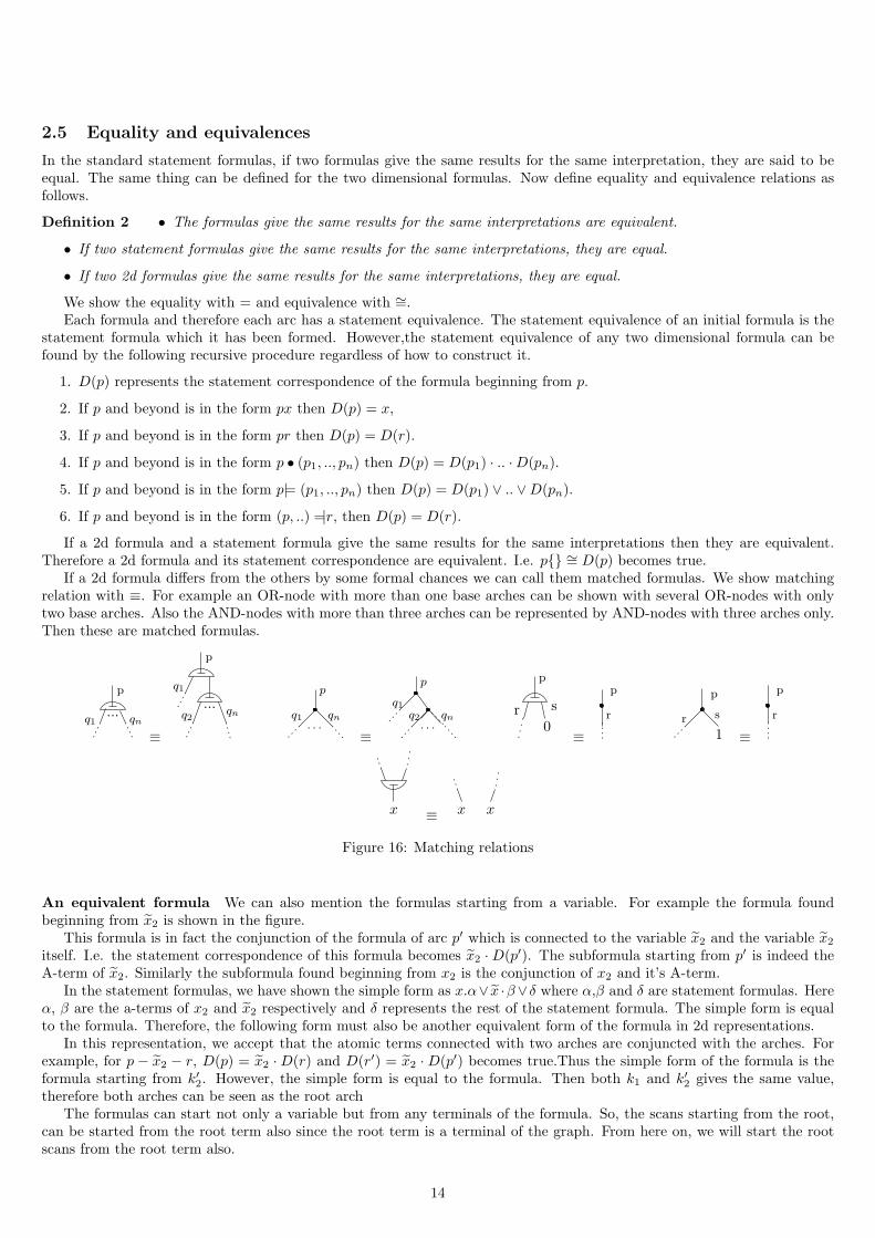
2.4 A notation

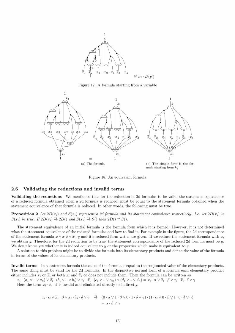
Let use instead of (1V..V 1) and instead of −1−.The formulas given in the figure is redrawn with this notation and shown in the figure.We want to express a two dimensional formula by means of its arches and nodes. Due to this new notation, we will write

the nodes as follows. p• (p1, .., pn) represents an AND-node where p is the incoming arc and p1, .., pn are the outgoing arches.p|= (p1, .., pn) represents an OR-node where p is the incoming arc and p1, .., pn are the outgoing arches. Naturally, the nodep • (r, s) can be written as r′ • (p′, s) or s′ • (p′, r). Similarly, the node p|= (p1, .., pn) can be written as (p′1, .., p

′n) =|p′.

11

1

(1V1V1V1)1

(1V1)

x4

(1V1)(1V1)

0

1(1V1)

1

x1

(1V1)

1 x1

1

1

k

1

1

1

1 1

(a) For |x2| = 1, |k| = 1

1

(1V1V1V1)

(1V1)

1

(1V1)(1V1)

1

1(1V1)

1

x1

(1V1)

0 x1

1

1

1

1

1

1

1

1

1

11

1

11

1

1

k

1 1

(b) For |x2| = 0 and |x4| = 1, |k| = 1

1

(1V1V1V1)1

(1V1)

0

(1V1)(1V1)

1

1(1V1)

1

x1

(1V1)

0 x1

1

1

k

0

0

0

00

0

0

0

0

0

0

0

1 1

(c) For |x2| = 0 and |x4| = 0, |k| = 0

Figure 11: The interpretations for the reduced formula. The values of arches which does not affect the result are not shown

1

(1V1V1V1)1

(1V1)

0

(1V1)(1V1)

1(1V1)

1

(1V1)

1

1

Figure 12: The totally reduced form of the example formula

1

x2 x3 x2 x4x1 x3x1

1

0

Figure 13: The sample formula and its last reduced form redrawn with new notation

p

r s

(a) Denoted as p • (r, s)or r′•(p′, s) or s′•(p′, r)

p

r s

(b) Denoted as p| =(r, s) or (r′, s′) =|p′

Figure 14: Node illustrations

Formulas of arches . Let the formula of an arc p be represented by p(). Each formula can be thought as composedof other formulas. Each formula is either a atomic term or an disjunction or an conjunction. An AND-node represents a

12

conjunction and an OR-node represents an disjunction. If p is tied to an AND-node then p() is a conjunction, if it is themain arc of an OR-node then it is a disjunction. For example y3 is tied to an AND-node whose arches directed to outside isy9 and y10. For this reason y3() is a conjunction and the elements of this conjunction is y9() and y10().

Then we can apply the following rules for the statement equivalences

1. The formula of p be p().

2. If p and beyond is in the form px then p() = px,

3. If p and beyond is in the form pr then p() = pr().

4. p and beyond is in the form p • (p1, .., pn) then p() = p • {p1(), .., pn()}.

5. p and beyond is in the form p|= (p1, .., pn) then p() = p|= {p1(), .., pn()}.

6. p and beyond is in the form p =|r then p() = p =|r().

For example for the subformula given in the figure and begins from y3, some equivalences would be valid.

1

x1 x2 x3 x2 x4x1 x3

y3

y4y1

y5 y6y7 y8

y9 y11y12 y13

y15 y16 y17 y18 y19 y20

y21

k

y10 y14

y2

Figure 15: subformula for y3

From here

y3() = y3 • {y12(), y19(), y13()}= y3 • {y12 =|y18(), y19x1, y13 =|y20()}= y3 • {y12 =|y18x2, y19x1, y13 =|y20x3}

is found. The reason to choose such a notation is that when the parenthesis are opened, then we get the paths of theformula. For example the path set of y3 would be found as

y3{} = {y3 • y12 =|y18x2, y3 • y19x1, y3 • y13 =|y20x3}

Paths The ways used to go from one element to another one is known as paths. A path is shown by writing arches,nodesand atomicss in sequence. For example, the path begin with p1 and end with x2 is written as p1|= p2 • y9 =|y17x2. Here |=represents a head-to-base or-node between the arches p1 and p2. Similarly • and =| represents an and node and a base-to-heador-node. The direction of path is from left to right. If we do not need to describe the types of nodes , we use the notation p.r.Here it is indicated that there is a node between p and r. Two subsequent arches are tied to each other with an and-node.So if r immediately comes after p we will write this as p • r or pr. Naturally several subsequent arches can be thought asone arc and one arc can be thought as composed of several subsequent arches. We will use both accordingly.

For each path there is a reverse path. For example the reverse of p1|= p2 • y9 =|y17x2 is x2y′17|= y′9 • p′2 =|y′1. |= and =|

are the reverse of each other. The reverse of a variable such as x is itself. the reverse of • is • again.The notation pAr shows a path which begins with p and end with r. The paths are shown with capital letters. The

reverse of the path pAr is written as r′A′p′. On the other hand, the notation p..r shows any path begins with p and endwith r. The reverse of them are shown as r′..p′. p.. and ..r shows the paths beginning with p and the paths end with rrespectively.

The path relation is transitive. I.e if p..r and r..s exist then a path p..r..s exists.If a path begins with a atomic term and end with an atomic term then it is a complete path. For example in a non-reduced

formula any path begins with root 1 and end with a variable is a complete path. The paths not complete can be calledsubpaths.

13

2.5 Equality and equivalences

In the standard statement formulas, if two formulas give the same results for the same interpretation, they are said to beequal. The same thing can be defined for the two dimensional formulas. Now define equality and equivalence relations asfollows.

Definition 2 • The formulas give the same results for the same interpretations are equivalent.

• If two statement formulas give the same results for the same interpretations, they are equal.

• If two 2d formulas give the same results for the same interpretations, they are equal.

We show the equality with = and equivalence with ∼=.Each formula and therefore each arc has a statement equivalence. The statement equivalence of an initial formula is the

statement formula which it has been formed. However,the statement equivalence of any two dimensional formula can befound by the following recursive procedure regardless of how to construct it.

1. D(p) represents the statement correspondence of the formula beginning from p.

2. If p and beyond is in the form px then D(p) = x,

3. If p and beyond is in the form pr then D(p) = D(r).

4. If p and beyond is in the form p • (p1, .., pn) then D(p) = D(p1) · .. ·D(pn).

5. If p and beyond is in the form p|= (p1, .., pn) then D(p) = D(p1) ∨ .. ∨D(pn).

6. If p and beyond is in the form (p, ..) =|r, then D(p) = D(r).

If a 2d formula and a statement formula give the same results for the same interpretations then they are equivalent.Therefore a 2d formula and its statement correspondence are equivalent. I.e. p{} ∼= D(p) becomes true.

If a 2d formula differs from the others by some formal chances we can call them matched formulas. We show matchingrelation with ≡. For example an OR-node with more than one base arches can be shown with several OR-nodes with onlytwo base arches. Also the AND-nodes with more than three arches can be represented by AND-nodes with three arches only.Then these are matched formulas.

...q1 qn

p

≡

...

q1

q2 qn

p

q1· · ·

qn

p

≡qn

· · ·q2

q1

p

0

p

r s

≡

p

r

1

p

r s

≡

p

r

x ≡ x x

Figure 16: Matching relations

An equivalent formula We can also mention the formulas starting from a variable. For example the formula foundbeginning from x2 is shown in the figure.

This formula is in fact the conjunction of the formula of arc p′ which is connected to the variable x2 and the variable x2

itself. I.e. the statement correspondence of this formula becomes x2 ·D(p′). The subformula starting from p′ is indeed theA-term of x2. Similarly the subformula found beginning from x2 is the conjunction of x2 and it’s A-term.

In the statement formulas, we have shown the simple form as x.α∨ x ·β∨δ where α,β and δ are statement formulas. Hereα, β are the a-terms of x2 and x2 respectively and δ represents the rest of the statement formula. The simple form is equalto the formula. Therefore, the following form must also be another equivalent form of the formula in 2d representations.

In this representation, we accept that the atomic terms connected with two arches are conjuncted with the arches. Forexample, for p − x2 − r, D(p) = x2 ·D(r) and D(r′) = x2 ·D(p′) becomes true.Thus the simple form of the formula is theformula starting from k′2. However, the simple form is equal to the formula. Then both k1 and k′2 gives the same value,therefore both arches can be seen as the root arch

The formulas can start not only a variable but from any terminals of the formula. So, the scans starting from the root,can be started from the root term also since the root term is a terminal of the graph. From here on, we will start the rootscans from the root term also.

14

1

x1 x2 x3 x2 x4x1 x3

p

∼= x2 ·D(p′)

Figure 17: A formula starting from a variable

1

x1 x2 x3 x2 x4x1 x3

k1

1k2

=

1

x1 x2 x3 x2 x4x1 x3

1

k1

k2

(a) The formula

1

x1 x2 x3 x2 x4x1 x3

1

k1

k2

(b) The simple form is the for-mula starting from k′2

Figure 18: An equivalent formula

2.6 Validating the reductions and invalid terms

Validating the reductions We mentioned that for the reduction in 2d formulas to be valid, the statement equivalenceof a reduced formula obtained when a 2d formula is reduced, must be equal to the statement formula obtained when thestatement equivalence of that formula is reduced. In other words, the following must be true.

Proposition 2 Let 2D(xi) and S(xi) represent a 2d formula and its statement equivalence respectively. I.e. let 2D(xi) ∼=S(xi) be true. If 2D(xi)

xi→ 2D() and S(xi)xi→ S() then 2D() ∼= S().

The statement equivalence of an initial formula is the formula from which it is formed. However, it is not determinedwhat the statement equivalence of the reduced formulas and how to find it. For example in the figure, the 2d correspondenceof the statement formula x ∨ x.x ∨ x · y and it’s reduced form wrt x are given. If we reduce the statement formula with x,we obtain y. Therefore, for the 2d reduction to be true, the statement correspondence of the reduced 2d formula must be y.We don’t know yet whether it is indeed equivalent to y or the properties which make it equivalent to y

A solution to this problem might be to divide the formula into its elementary products and define the value of the formulain terms of the values of its elementary products.

Invalid terms In a statement formula the value of the formula is equal to the conjuncted value of the elementary products.The same thing must be valid for the 2d formulas. In the disjunctive normal form of a formula each elementary producteither includes xi or xi or both xi and xi or does not include them. Then the formula can be written as

xi · (a1 ∨ .. ∨ ak) ∨ xi · (b1 ∨ .. ∨ bl) ∨ xi · xi · (c1 ∨ .. ∨ cm) ∨ (d1 ∨ .. ∨ dn) = xi · α ∨ xi · β ∨ xi · xi · δ ∨ γHere the term xi · xi · δ is invalid and eliminated directly or indirectly.

xi · α ∨ xi · β ∨ xi · xi · δ ∨ γxi→ (0 · α ∨ 1 · β ∨ 0 · 1 · δ ∨ γ) · (1 · α ∨ 0 · β ∨ 1 · 0 · δ ∨ γ)

= α · β ∨ γ

15

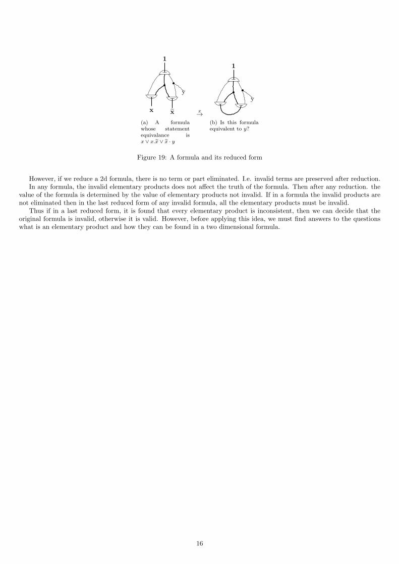
1

y

xx

(a) A formulawhose statementequivalance isx ∨ x.x ∨ x · y

x→

1

y

(b) Is this formulaequivalent to y?

Figure 19: A formula and its reduced form

However, if we reduce a 2d formula, there is no term or part eliminated. I.e. invalid terms are preserved after reduction.In any formula, the invalid elementary products does not affect the truth of the formula. Then after any reduction. the

value of the formula is determined by the value of elementary products not invalid. If in a formula the invalid products arenot eliminated then in the last reduced form of any invalid formula, all the elementary products must be invalid.

Thus if in a last reduced form, it is found that every elementary product is inconsistent, then we can decide that theoriginal formula is invalid, otherwise it is valid. However, before applying this idea, we must find answers to the questionswhat is an elementary product and how they can be found in a two dimensional formula.

16

Part II

Elementary products and scans

17

3 Initial formulas and elementary products

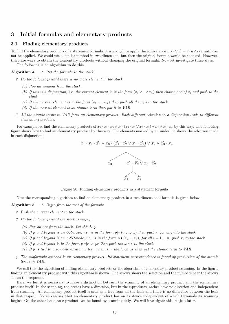
3.1 Finding elementary products

To find the elementary products of a statement formula, it is enough to apply the equivalence x · (y∨z) = x ·y∨x ·z until cannot be applied. We could use a similar method in two dimension, but then the original formula would be changed. However,there are ways to obtain the elementary products without changing the original formula. Now let investigate these ways.

The following is an algorithm to do this.

Algorithm 4 1. Put the formula to the stack.

2. Do the followings until there is no more element in the stack.

(a) Pop an element from the stack.

(b) If this is a disjunction, i.e. the current element is in the form (a1 ∨ ..∨ an) then choose one of ai and push to thestack.

(c) If the current element is in the form (a1 · .. · an) then push all the ai’s to the stack.

(d) If the current element is an atomic term then put it to VAR.

3. All the atomic terms in VAR form an elementary product. Each different selection in a disjunction leads to differentelementary products.

For example let find the elementary products of x1 ·x2 · x3 ∨x3 · (x1 · x2 ∨x3 · x2)∨x2 ∨ x3 ·x4 by this way. The followingfigure shows how to find an elementary product by this way. The elements marked by an underline shows the selection madein each disjunction.

x1 · x2 · x3 ∨ x3 · (x1 · x2 ∨ x3 · x2) ∨ x2 ∨ x3 · x4

x3 x1 · x2 ∨ x3 · x2

x1 x2

Figure 20: Finding elementary products in a statement formula

Now the corresponding algorithm to find an elementary product in a two dimensional formula is given below.

Algorithm 5 1. Begin from the root of the formula

2. Push the current element to the stack.

3. Do the followings until the stack is empty.

(a) Pop an arc from the stack. Let this be p.

(b) If p and beyond is an OR-node, i.e. is in the form p|= (r1, .., rn) then push ri for any i to the stack.

(c) If p and beyond is an AND-node, i.e. is in the form p • (r1, .., rn), for all i = 1, .., n, push ri to the stack.

(d) If p and beyond is in the form p =|r or pr then push the arc r to the stack.

(e) If p is tied to a variable or atomic term, i.e. is in the form px then put the atomic term to VAR.

4. The subformula scanned is an elementary product. Its statement correspondence is found by production of the atomicterms in VAR.

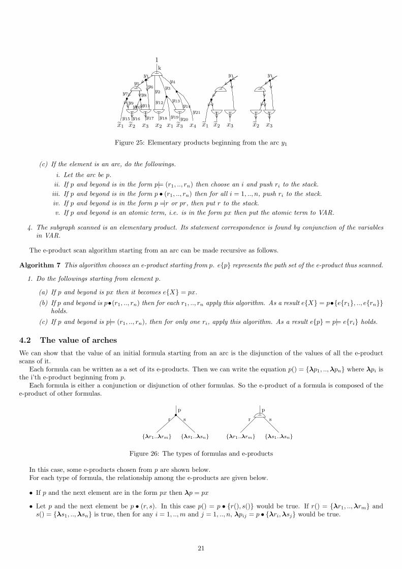
We call this the algorithm of finding elementary products or the algorithm of elementary product scanning. In the figure,finding an elementary product with this algorithm is shown. The arrows shows the selection and the numbers near the arrowsshows the sequence.

Here, we feel it is necessary to make a distinction between the scanning of an elementary product and the elementaryproduct itself. In the scanning, the arches have a direction, but in the e-products, arches have no direction and independentfrom scanning. An elementary product itself is seen as a tree from all the leafs and there is no difference between the leafsin that respect. So we can say that an elementary product has an existence independent of which terminals its scanningbegins. On the other hand an e-product can be found by scanning only. We will investigate this subject later.

18

1

x1 x2 x3 x2 x4x1 x3

(a) The scanning

1

x1 x2 x3

(b) the e-product found

Figure 21: Scanning of an e-product in a two dimensional formula

Figure 22: An e-product is seems the same from every terminals and can be found with a single scanning

3.2 Simple and elementary product scans

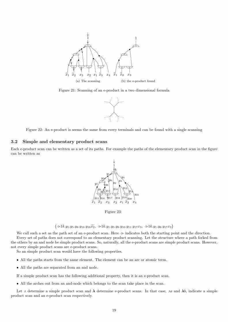
Each e-product scan can be written as a set of its paths. For example the paths of the elementary product scan in the figurecan be written as

x1 x2 x3 x2 x4x1 x3

y3

y4y1

y5 y6y7 y8

y9 y11y12 y13

y15 y16 y17 y18 y19 y20

y21

k

y10 y14

y2

1

Figure 23:

{−>1k.y1.y5.y8.y10.y16x2, −>1k.y1.y5.y8.y10.y11.y17x3, −>1k.y1.y6.y17x3}

We call such a set as the path set of an e-product scan. Here −> indicates both the starting point and the direction.Every set of paths does not correspond to an elementary product scanning. Let the structure where a path forked from

the others by an and node be simple product scans. So, naturally, all the e-product scans are simple product scans. However,not every simple product scans are e-product scans.

So an simple product scan would have the following properties.

• All the paths starts from the same element. The element can be an arc or atomic term.

• All the paths are separated from an and node.

If a simple product scan has the following additional property, then it is an e-product scan.

• All the arches out from an and-node which belongs to the scan take place in the scan.

Let ⋏ determine a simple product scan and λ determine e-product scans. In that case, ⋏a and λb, indicate a simpleproduct scan and an e-product scan respectively.

19

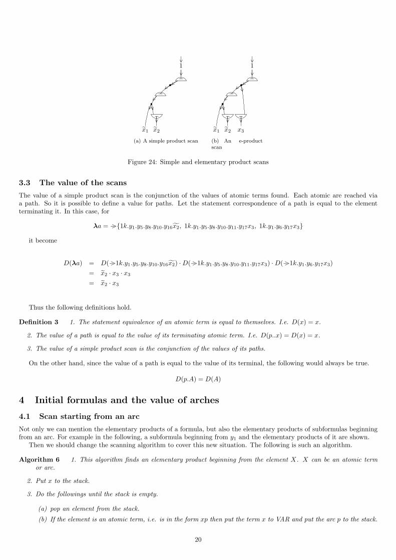
1

x1 x2

(a) A simple product scan

1

x1 x2 x3

(b) An e-productscan

Figure 24: Simple and elementary product scans

3.3 The value of the scans

The value of a simple product scan is the conjunction of the values of atomic terms found. Each atomic are reached viaa path. So it is possible to define a value for paths. Let the statement correspondence of a path is equal to the elementterminating it. In this case, for

λa = −>{1k.y1.y5.y8.y10.y16x2, 1k.y1.y5.y8.y10.y11.y17x3, 1k.y1.y6.y17x3}

it become

D(λa) = D(−>1k.y1.y5.y8.y10.y16x2) ·D(−>1k.y1.y5.y8.y10.y11.y17x3) ·D(−>1k.y1.y6.y17x3)

= x2 · x3 · x3

= x2 · x3

Thus the following definitions hold.

Definition 3 1. The statement equivalence of an atomic term is equal to themselves. I.e. D(x) = x.

2. The value of a path is equal to the value of its terminating atomic term. I.e. D(p..x) = D(x) = x.

3. The value of a simple product scan is the conjunction of the values of its paths.

On the other hand, since the value of a path is equal to the value of its terminal, the following would always be true.

D(p.A) = D(A)

4 Initial formulas and the value of arches

4.1 Scan starting from an arc

Not only we can mention the elementary products of a formula, but also the elementary products of subformulas beginningfrom an arc. For example in the following, a subformula beginning from y1 and the elementary products of it are shown.

Then we should change the scanning algorithm to cover this new situation. The following is such an algorithm.

Algorithm 6 1. This algorithm finds an elementary product beginning from the element X. X can be an atomic termor arc.

2. Put x to the stack.

3. Do the followings until the stack is empty.

(a) pop an element from the stack.

(b) If the element is an atomic term, i.e. is in the form xp then put the term x to VAR and put the arc p to the stack.

20

1

x1 x2 x3 x2 x4x1 x3

y3

y4y1

y5 y6y7 y8

y9 y11y12 y13

y15 y16 y17 y18 y19 y20

y21

k

y10 y14

y2

x1 x2 x3

y1

x2 x3

y1

Figure 25: Elementary products beginning from the arc y1

(c) If the element is an arc, do the followings.

i. Let the arc be p.

ii. If p and beyond is in the form p|= (r1, .., rn) then choose an i and push ri to the stack.

iii. If p and beyond is in the form p • (r1, .., rn) then for all i = 1, .., n, push ri to the stack.

iv. If p and beyond is in the form p =|r or pr, then put r to the stack.

v. If p and beyond is an atomic term, i.e. is in the form px then put the atomic term to VAR.

4. The subgraph scanned is an elementary product. Its statement correspondence is found by conjunction of the variablesin VAR.

The e-product scan algorithm starting from an arc can be made recursive as follows.

Algorithm 7 This algorithm chooses an e-product starting from p. e{p} represents the path set of the e-product thus scanned.

1. Do the followings starting from element p.

(a) If p and beyond is px then it becomes e{X} = px.

(b) If p and beyond is p•(r1, .., rn) then for each r1, .., rn apply this algorithm. As a result e{X} = p•{e{r1}, .., e{rn}}holds.

(c) If p and beyond is p|= (r1, .., rn), then for only one ri, apply this algorithm. As a result e{p} = p|= e{ri} holds.

4.2 The value of arches

We can show that the value of an initial formula starting from an arc is the disjunction of the values of all the e-productscans of it.

Each formula can be written as a set of its e-products. Then we can write the equation p() = {λp1, ..,λpn} where λpi isthe i’th e-product beginning from p.

Each formula is either a conjunction or disjunction of other formulas. So the e-product of a formula is composed of thee-product of other formulas.

{λr1..λrm} {λs1..λsn}

r s

p

{λr1..λrm} {λs1..λsn}

s

p

r

Figure 26: The types of formulas and e-products

In this case, some e-products chosen from p are shown below.For each type of formula, the relationship among the e-products are given below.

• If p and the next element are in the form px then λp = px

• Let p and the next element be p • (r, s). In this case p() = p • {r(), s()} would be true. If r() = {λr1, ..,λrm} ands() = {λs1, ..,λsn} is true, then for any i = 1, ..,m and j = 1, .., n, λpij = p • {λri,λsj} would be true.

21

{λr1..λrm} {λs1..λsn}

p

sr

λp11 = p • {λr1,λs1}

{λr1..λrm} {λs1..λsn}

s

p

r

λp1 = p|= λr1

{�r1.. � rm} {λs1..λsn}

s

p

r

λpm+1 = p|= λs1

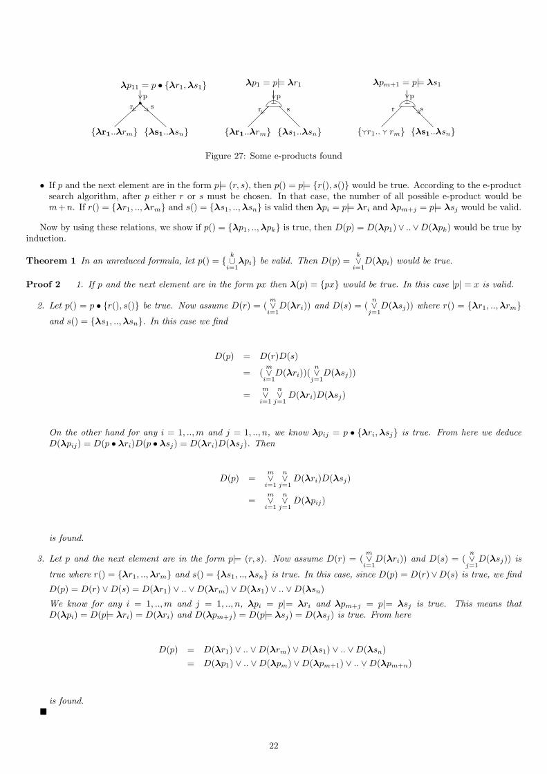
Figure 27: Some e-products found

• If p and the next element are in the form p|= (r, s), then p() = p|= {r(), s()} would be true. According to the e-productsearch algorithm, after p either r or s must be chosen. In that case, the number of all possible e-product would bem+n. If r() = {λr1, ..,λrm} and s() = {λs1, ..,λsn} is valid then λpi = p|= λri and λpm+j = p|= λsj would be valid.

Now by using these relations, we show if p() = {λp1, ..,λpk} is true, then D(p) = D(λp1)∨ ..∨D(λpk) would be true byinduction.

Theorem 1 In an unreduced formula, let p() = {k∪i=1

λpi} be valid. Then D(p) =k∨i=1

D(λpi) would be true.

Proof 2 1. If p and the next element are in the form px then λ(p) = {px} would be true. In this case |p| = x is valid.

2. Let p() = p • {r(), s()} be true. Now assume D(r) = (m∨i=1

D(λri)) and D(s) = (n∨

j=1D(λsj)) where r() = {λr1, ..,λrm}

and s() = {λs1, ..,λsn}. In this case we find

D(p) = D(r)D(s)

= (m∨i=1

D(λri))(n∨

j=1D(λsj))

=m∨i=1

n∨

j=1D(λri)D(λsj)

On the other hand for any i = 1, ..,m and j = 1, .., n, we know λpij = p • {λri,λsj} is true. From here we deduceD(λpij) = D(p • λri)D(p • λsj) = D(λri)D(λsj). Then

D(p) =m∨i=1

n∨

j=1D(λri)D(λsj)

=m∨i=1

n∨

j=1D(λpij)

is found.

3. Let p and the next element are in the form p|= (r, s). Now assume D(r) = (m∨i=1

D(λri)) and D(s) = (n∨

j=1D(λsj)) is

true where r() = {λr1, ..,λrm} and s() = {λs1, ..,λsn} is true. In this case, since D(p) = D(r)∨D(s) is true, we find

D(p) = D(r) ∨D(s) = D(λr1) ∨ .. ∨D(λrm) ∨D(λs1) ∨ .. ∨D(λsn)

We know for any i = 1, ..,m and j = 1, .., n, λpi = p|= λri and λpm+j = p|= λsj is true. This means thatD(λpi) = D(p|= λri) = D(λri) and D(λpm+j) = D(p|= λsj) = D(λsj) is true. From here

D(p) = D(λr1) ∨ .. ∨D(λrm) ∨D(λs1) ∨ .. ∨D(λsn)

= D(λp1) ∨ .. ∨D(λpm) ∨D(λpm+1) ∨ .. ∨D(λpm+n)

is found.■

22

5 Symmetry in e-products and regular formulas

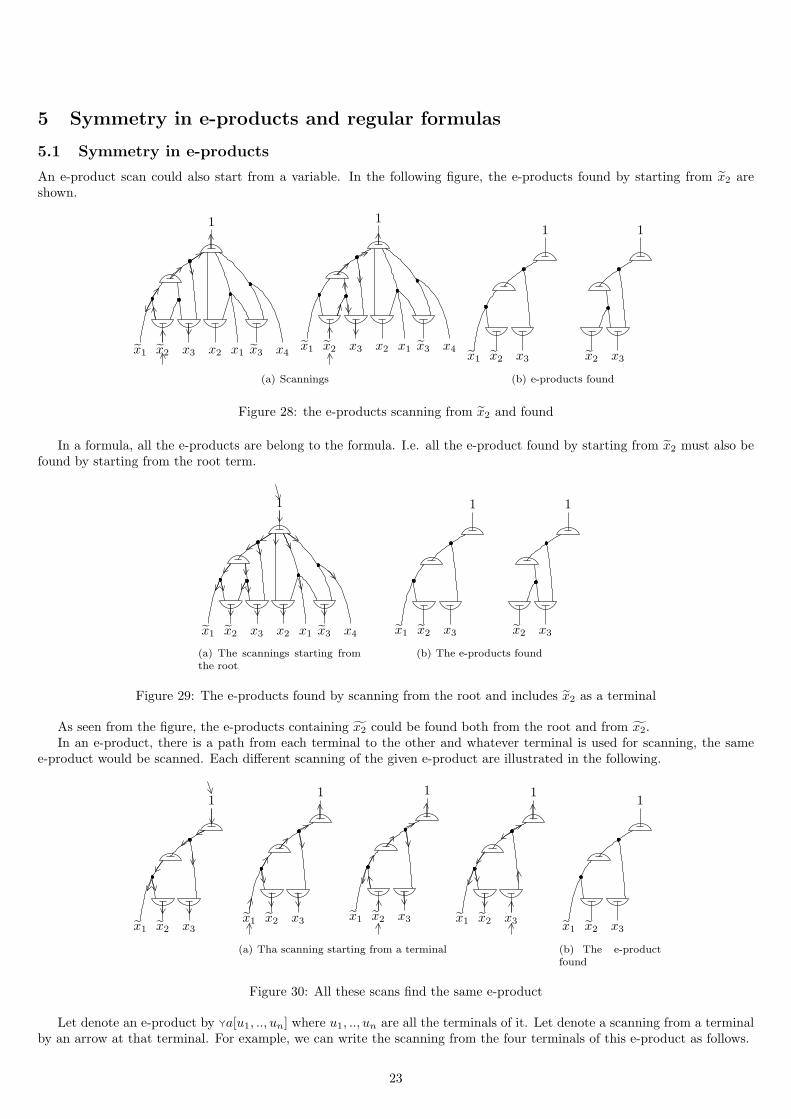
5.1 Symmetry in e-products

An e-product scan could also start from a variable. In the following figure, the e-products found by starting from x2 areshown.

1

x1 x2 x3 x2 x4x1 x3

1

x2 x3 x2 x4x1 x3x1

(a) Scannings

1

x1 x2 x3

1

x2 x3

(b) e-products found

Figure 28: the e-products scanning from x2 and found

In a formula, all the e-products are belong to the formula. I.e. all the e-product found by starting from x2 must also befound by starting from the root term.

1

x1 x2 x3 x2 x4x1 x3

(a) The scannings starting fromthe root

1

x1 x2 x3

1

x2 x3

(b) The e-products found

Figure 29: The e-products found by scanning from the root and includes x2 as a terminal

As seen from the figure, the e-products containing x2 could be found both from the root and from x2.In an e-product, there is a path from each terminal to the other and whatever terminal is used for scanning, the same

e-product would be scanned. Each different scanning of the given e-product are illustrated in the following.

1

x1 x2 x3

1

x1 x2 x3

1

x1 x2 x3

1

x1 x2 x3

(a) Tha scanning starting from a terminal

1

x1 x2 x3

(b) The e-productfound

Figure 30: All these scans find the same e-product

Let denote an e-product by �a[u1, .., un] where u1, .., un are all the terminals of it. Let denote a scanning from a terminalby an arrow at that terminal. For example, we can write the scanning from the four terminals of this e-product as follows.

23

λa1 = �a[−>1, x1, x2, x3]

λa2 = �a[1,−>x1, x2, x3]

λa3 = �a[1, x1,−>x2, x3]

λa4 = �a[1, x1, x2,−>x3]

Each e-product has an statement equivalence. The value of an e-product is the conjunction of the values of its terminals.For example

D(�a[1, x1, x2, x3]) = 1 · x1 · x2 · x3

. However as seen, an e-product can be found by scanning only from a single terminal because there is a path from everyterminal to the others and a single scanning finds all the terminals. In this case, the value of each scanning would be thesame and give the value of the e-product. In other words the following would be true.

D(�a) = D(λa1) = D(λa2) = D(λa3) = D(λa4)

Scannings of an e-product In an e-product, we can determine all the other scans from one scanning. Also all these scansmust give the same value. Let there are terminals xi and xj in an e-product. Thus, there is a path xiAxj in the scanningstarting from xi. Let show such a scan having such a path as in the figure.

xi xj

p q s

tr

Figure 31: A scan having the path xiAxj

However, in this case, there exists a scanning which starts from xj , has the path xjA′xi and where all the arches of it,

except the arches on A and A′, are the same with the above scanning.

xi xj

p q s

tr

Figure 32: There is another e-product scan which has the path xjA′xi

Let call the second scanning the reverse scanning over the path xiAxj . This means that, each scan has reverse scans overeach of its paths and all of these scans has the same terminals. Therefore they have the same value. So an e-product scanand it’s all reverse scans determines the same e-product. This is true for every scan of an e-product. I.e. each scan of ane-product is a reverse scan of all the others.

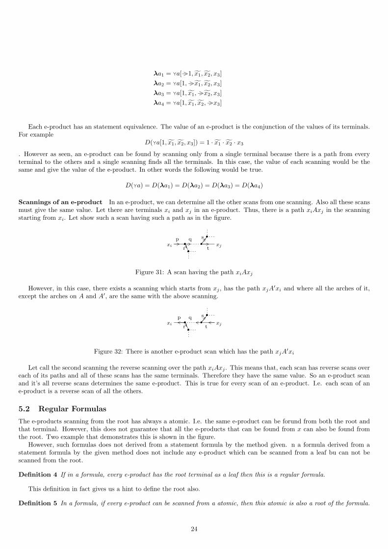
5.2 Regular Formulas

The e-products scanning from the root has always a atomic. I.e. the same e-product can be forund from both the root andthat terminal. However, this does not guarantee that all the e-products that can be found from x can also be found fromthe root. Two example that demonstrates this is shown in the figure.

However, such formulas does not derived from a statement formula by the method given. n a formula derived from astatement formula by the given method does not include any e-product which can be scanned from a leaf bu can not bescanned from the root.

Definition 4 If in a formula, every e-product has the root terminal as a leaf then this is a regular formula.

This definition in fact gives us a hint to define the root also.

Definition 5 In a formula, if every e-product can be scanned from a atomic, then this atomic is also a root of the formula.

24

x x

y

1

x x

1

Figure 33: e-products that can be scanned from x, but can not be scanned from the root

x2 x3 x2 x3

k1

1

1

x1 x4x1

k2

x2 x3 x2 x3

k1

1

1

x1 x4x1

k2

(a) Formulas with two root terms

x1 x2 x3 x2 x4x1 x3

1

(b) The formula without a rootterm

Figure 34: Formulas can have any number of root terms

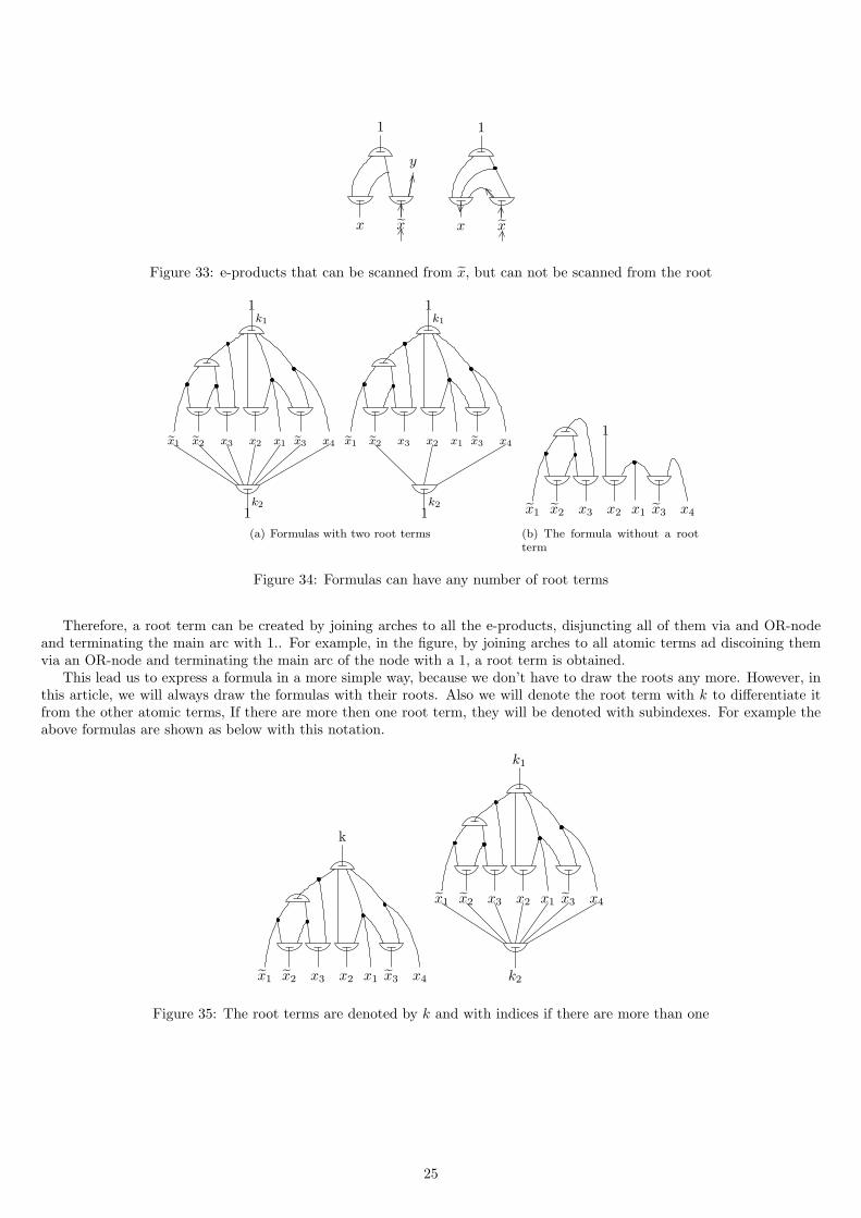
Therefore, a root term can be created by joining arches to all the e-products, disjuncting all of them via and OR-nodeand terminating the main arc with 1.. For example, in the figure, by joining arches to all atomic terms ad discoining themvia an OR-node and terminating the main arc of the node with a 1, a root term is obtained.

This lead us to express a formula in a more simple way, because we don’t have to draw the roots any more. However, inthis article, we will always draw the formulas with their roots. Also we will denote the root term with k to differentiate itfrom the other atomic terms, If there are more then one root term, they will be denoted with subindexes. For example theabove formulas are shown as below with this notation.

k

x2 x3 x2 x4x1 x3x1

k1

x1 x2 x3 x2 x4x1 x3

k2

Figure 35: The root terms are denoted by k and with indices if there are more than one

25

6 Reduced formulas and e-product scanning

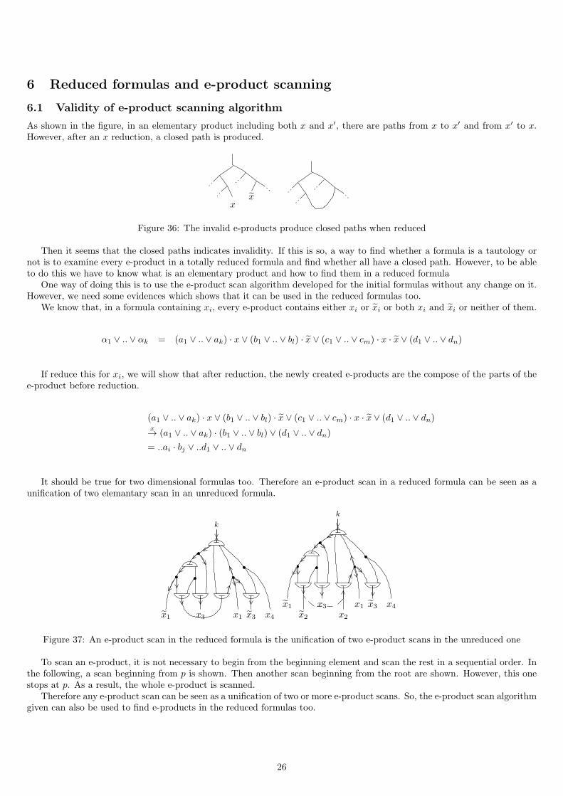
6.1 Validity of e-product scanning algorithm

As shown in the figure, in an elementary product including both x and x′, there are paths from x to x′ and from x′ to x.However, after an x reduction, a closed path is produced.

xx

Figure 36: The invalid e-products produce closed paths when reduced

Then it seems that the closed paths indicates invalidity. If this is so, a way to find whether a formula is a tautology ornot is to examine every e-product in a totally reduced formula and find whether all have a closed path. However, to be ableto do this we have to know what is an elementary product and how to find them in a reduced formula

One way of doing this is to use the e-product scan algorithm developed for the initial formulas without any change on it.However, we need some evidences which shows that it can be used in the reduced formulas too.

We know that, in a formula containing xi, every e-product contains either xi or xi or both xi and xi or neither of them.

α1 ∨ .. ∨ αk = (a1 ∨ .. ∨ ak) · x ∨ (b1 ∨ .. ∨ bl) · x ∨ (c1 ∨ .. ∨ cm) · x · x ∨ (d1 ∨ .. ∨ dn)

If reduce this for xi, we will show that after reduction, the newly created e-products are the compose of the parts of thee-product before reduction.

(a1 ∨ .. ∨ ak) · x ∨ (b1 ∨ .. ∨ bl) · x ∨ (c1 ∨ .. ∨ cm) · x · x ∨ (d1 ∨ .. ∨ dn)x→ (a1 ∨ .. ∨ ak) · (b1 ∨ .. ∨ bl) ∨ (d1 ∨ .. ∨ dn)

= ..ai · bj ∨ ..d1 ∨ .. ∨ dn

It should be true for two dimensional formulas too. Therefore an e-product scan in a reduced formula can be seen as aunification of two elemantary scan in an unreduced formula.

x1 x3 x1 x3 x4

k

k

x3 x1 x3 x4x1

x2 x2

Figure 37: An e-product scan in the reduced formula is the unification of two e-product scans in the unreduced one

To scan an e-product, it is not necessary to begin from the beginning element and scan the rest in a sequential order. Inthe following, a scan beginning from p is shown. Then another scan beginning from the root are shown. However, this onestops at p. As a result, the whole e-product is scanned.

Therefore any e-product scan can be seen as a unification of two or more e-product scans. So, the e-product scan algorithmgiven can also be used to find e-products in the reduced formulas too.

26

x3x2

k

p

(a)

x2 x3

k

p

(b)

k

x2 x3

p

(c)

Figure 38: An e-product can be scanned seperately

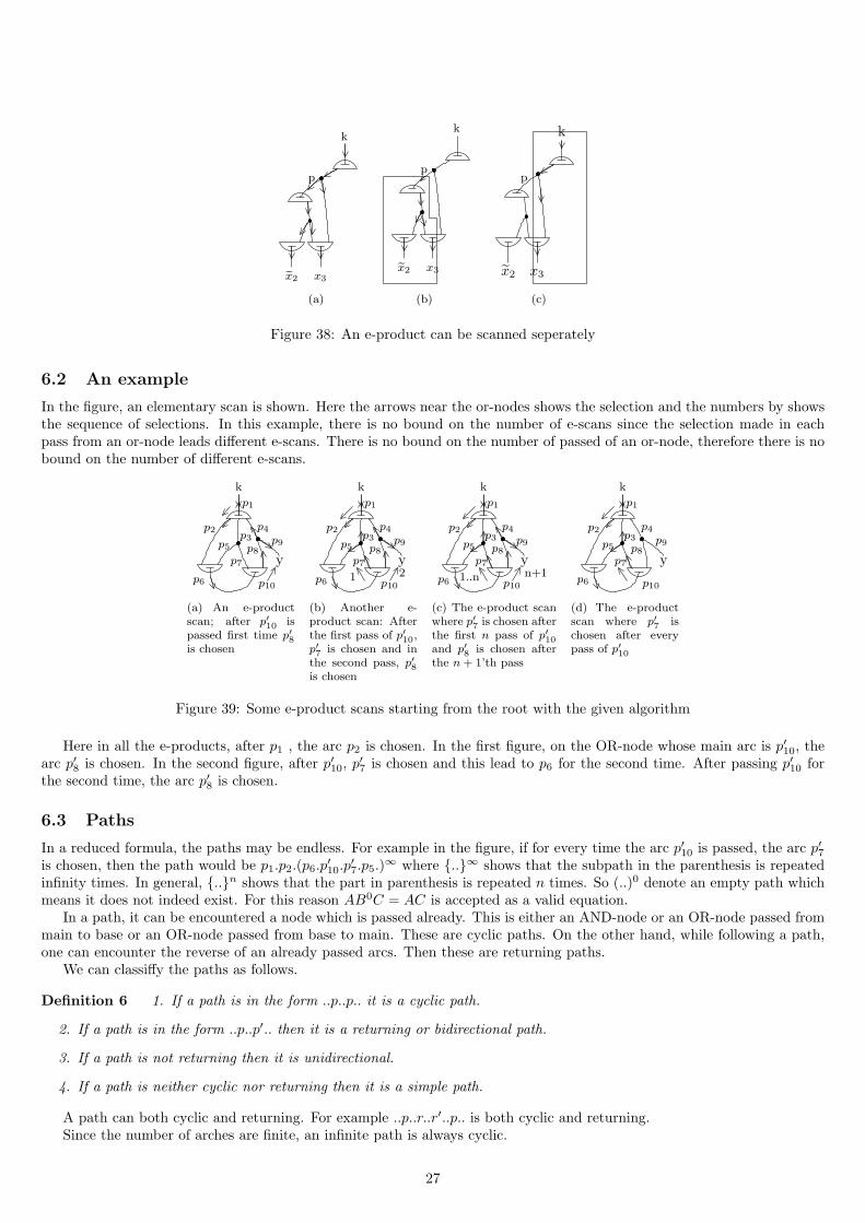
6.2 An example

In the figure, an elementary scan is shown. Here the arrows near the or-nodes shows the selection and the numbers by showsthe sequence of selections. In this example, there is no bound on the number of e-scans since the selection made in eachpass from an or-node leads different e-scans. There is no bound on the number of passed of an or-node, therefore there is nobound on the number of different e-scans.

k

p5

y

p9

p2

p1

p4

p6 p10

p7p8

p3

(a) An e-productscan; after p′10 ispassed first time p′8is chosen

k

p5

y

p9

p2

p1

p4

p6 p10

p7p8

p3

1 2

(b) Another e-product scan: Afterthe first pass of p′10,p′7 is chosen and inthe second pass, p′8is chosen

k

p5

y

p9

p2

p1

p4

p6 p10

p7p8

p3

n+11..n

(c) The e-product scanwhere p′7 is chosen afterthe first n pass of p′10and p′8 is chosen afterthe n+ 1’th pass

k

p5

y

p9

p2

p1

p4

p6 p10

p7p8

p3

(d) The e-productscan where p′7 ischosen after everypass of p′10

Figure 39: Some e-product scans starting from the root with the given algorithm

Here in all the e-products, after p1 , the arc p2 is chosen. In the first figure, on the OR-node whose main arc is p′10, thearc p′8 is chosen. In the second figure, after p′10, p

′7 is chosen and this lead to p6 for the second time. After passing p′10 for

the second time, the arc p′8 is chosen.

6.3 Paths

In a reduced formula, the paths may be endless. For example in the figure, if for every time the arc p′10 is passed, the arc p′7is chosen, then the path would be p1.p2.(p6.p

′10.p

′7.p5.)

∞ where {..}∞ shows that the subpath in the parenthesis is repeatedinfinity times. In general, {..}n shows that the part in parenthesis is repeated n times. So (..)0 denote an empty path whichmeans it does not indeed exist. For this reason AB0C = AC is accepted as a valid equation.

In a path, it can be encountered a node which is passed already. This is either an AND-node or an OR-node passed frommain to base or an OR-node passed from base to main. These are cyclic paths. On the other hand, while following a path,one can encounter the reverse of an already passed arcs. Then these are returning paths.

We can classiffy the paths as follows.

Definition 6 1. If a path is in the form ..p..p.. it is a cyclic path.

2. If a path is in the form ..p..p′.. then it is a returning or bidirectional path.

3. If a path is not returning then it is unidirectional.

4. If a path is neither cyclic nor returning then it is a simple path.

A path can both cyclic and returning. For example ..p..r..r′..p.. is both cyclic and returning.Since the number of arches are finite, an infinite path is always cyclic.

27

0 1 x

(a) paths endwith a atomicterm

(b) cyclic paths (c) returning paths

Figure 40: Types of paths

6.4 Paths and E-scans

An e-product scan beginning from an arc can be written as a set of paths beginning from that arc. For example the pathset of the e-product scan shown in the figure is given below.

λa = λ{−>kp1.p2.p6.p′10.p

′8 • p9y,−>kp1.p2.p6.p

′10.p

′8 • p′4.p′1k}

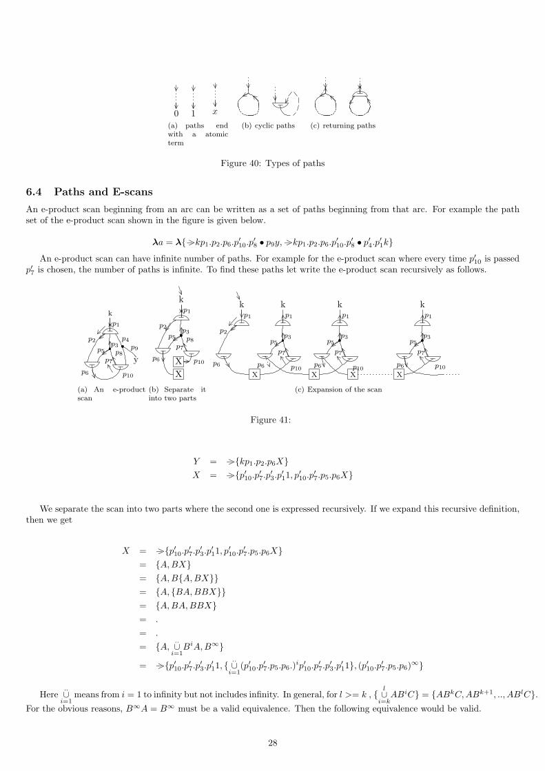
An e-product scan can have infinite number of paths. For example for the e-product scan where every time p′10 is passedp′7 is chosen, the number of paths is infinite. To find these paths let write the e-product scan recursively as follows.

k

p5

y

p9

p2

p1

p4

p6 p10

p7p8

p3

(a) An e-productscan

k

p5

p2

p1

p6 p10

p7

X

X

p8

p3

(b) Separate itinto two parts

p2

p1

p6

k

p5

p1

p7

p3

k

p5

p1

p10

p7

p3

k

p5

p1

p7

p3

p10p6 p10 p6 p6

k

X X X X

(c) Expansion of the scan

Figure 41:

Y = −>{kp1.p2.p6X}X = −>{p′10.p′7.p′3.p′11, p′10.p′7.p5.p6X}

We separate the scan into two parts where the second one is expressed recursively. If we expand this recursive definition,then we get

X = −>{p′10.p′7.p′3.p′11, p′10.p′7.p5.p6X}= {A,BX}= {A,B{A,BX}}= {A, {BA,BBX}}= {A,BA,BBX}= .

= .

= {A,..∪i=1

BiA,B∞}

= −>{p′10.p′7.p′3.p′11, {..∪i=1

(p′10.p′7.p5.p6.)

ip′10.p′7.p

′3.p

′11}, (p′10.p′7.p5.p6)∞}

Here..∪i=1

means from i = 1 to infinity but not includes infinity. In general, for l >= k , {l∪i=k

ABiC} = {ABkC,ABk+1, .., ABlC}.For the obvious reasons, B∞A = B∞ must be a valid equivalence. Then the following equivalence would be valid.

28

X = {A,..∪i=1

BiA,B∞} = {∞∪i=0

BiA}

where B0A = A. Therefore, the above set can be written as

λb = λ{∞∪i=0

−>(p′10.p′7.p5.p6)

ip′10.p′7.p

′3.p

′1k}

As in the initial formulas, we accept that the value of an e-product scan is the conjunction of the values of its paths.

6.5 Values of the arches

The value of a formula is the value of it’s root term or arc. Therefore we only need to find the value of arches in general toknow the value of the formulas.

We have shown that the value of an arch in an initial formula is equal to the disjunction of the values of the e-productscans starting from that arc. However, we can not prove a similar thing for reduced formulas by induction, because inreduced formulas there can be no end of the paths and therefore the necessity of induction can not be satisfied. On the otherhand, we can see this is true for reduced formula too by the following reasoning.

Theorem 2 Suppose the value of an arc is equal to the disjunction of the values of its e-product scans. This property doesnot change with reduction.

Proof 3 Consider the arches of the terms px and rx in a formula. Assume all of the arches p, r, p′, r′ have this property.Let reduce the formula for x. After reduction, the connection would be in the form ..pr′... If r′ still has this property, p wouldhave had this property by induction. However, there is no reason for r′ to loss this property by reduction. If there is no pathfrom r′ to p, this property of r′ does not affected by p. On the other hand, suppose there is a path pr′..p. In this case, thisproperty of p depends on itself. I.e. if we assume that p does not loss this property, by induction, p does not loss this propertyand it seems that there is no reason for p to loss this property. Therefore, for any arc in the formula, a reduction does notchange this property

On the other hand, whether we express this as a theorem or assumption is not important. We are totally free to make anyassumption and the only restricting factor here is whether the reduced formula keeps the tautological value of the originalone under these assumptions. If this is so, they can be used to identify tautology in two dimensional formulas. I.e, we canwrite this property as a postulate instead of a theorem.

Postulate 1 the value of an arc in any formula is equal to the disjunction of the values of all the e-product scans startingfrom that arc.

7 Elementary sums

7.1 E-sum scans

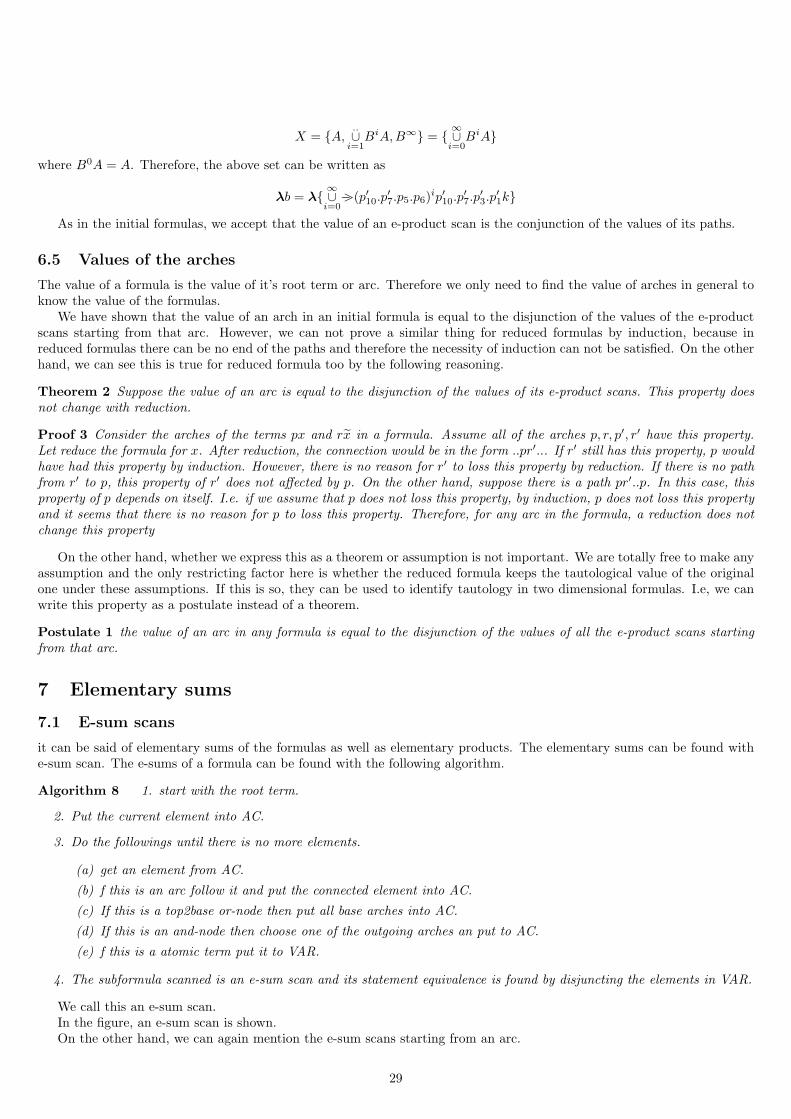
it can be said of elementary sums of the formulas as well as elementary products. The elementary sums can be found withe-sum scan. The e-sums of a formula can be found with the following algorithm.

Algorithm 8 1. start with the root term.

2. Put the current element into AC.

3. Do the followings until there is no more elements.

(a) get an element from AC.

(b) f this is an arc follow it and put the connected element into AC.

(c) If this is a top2base or-node then put all base arches into AC.

(d) If this is an and-node then choose one of the outgoing arches an put to AC.

(e) f this is a atomic term put it to VAR.

4. The subformula scanned is an e-sum scan and its statement equivalence is found by disjuncting the elements in VAR.

We call this an e-sum scan.In the figure, an e-sum scan is shown.On the other hand, we can again mention the e-sum scans starting from an arc.

29

k

x1 x2 x3 x2 x4x1 x3

k

x3 x2 x1 x3

k

x3 x2 x1 x3

Figure 42: An e-sum scan and the e-sum found

Algorithm 9 1. This algorithm find an e-sum scan starting from p

2. Put p into stack.

3. Repeat the following until the stack is empty.

(a) Pop an arc from the stack. Let this be p.

(b) If p and beyond is in the form p • (r1, .., rn) then for one i, push ri to the stack.

(c) If p and beyond is in the form p|= (r1, .., rn), then for i = 1, .., n, push ri to the stack.

(d) If p and beyond is in the form p =|r or pr, then push r to the stack.

(e) If p is connected to a atomic term, i.e. if p and beyond is in the form px, then put x into VAR.

4. The subformula scanned is an e-sum scan and its statement equivalence is found by disjuncting the elements in VAR..

As for the e-product scans, the value of the e-sum scan is defined as follows:”The value of an e-sum scan is the disjunction of the values of it’s paths.

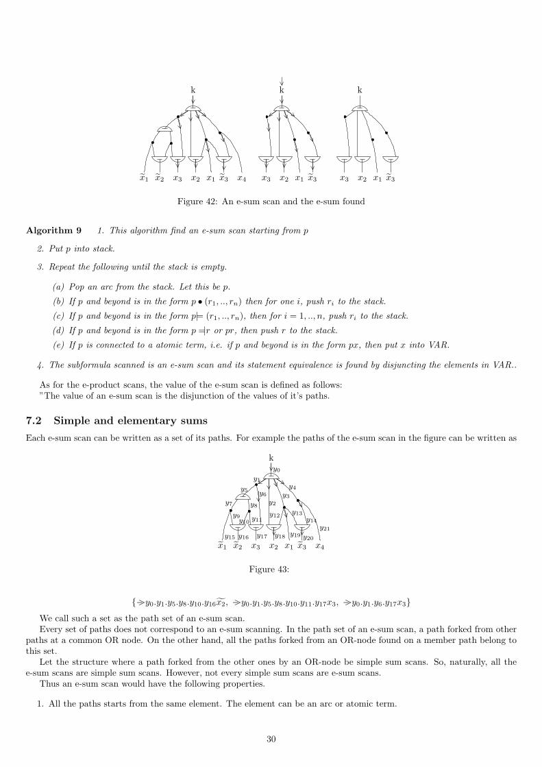
7.2 Simple and elementary sums

Each e-sum scan can be written as a set of its paths. For example the paths of the e-sum scan in the figure can be written as

k

x1 x2 x3 x2 x4x1 x3

y3

y4y1

y5 y6y7 y8

y9 y11y12 y13

y15 y16 y17 y18 y19 y20

y21

y0

y10 y14

y2

Figure 43:

{−>y0.y1.y5.y8.y10.y16x2, −>y0.y1.y5.y8.y10.y11.y17x3, −>y0.y1.y6.y17x3}

We call such a set as the path set of an e-sum scan.Every set of paths does not correspond to an e-sum scanning. In the path set of an e-sum scan, a path forked from other

paths at a common OR node. On the other hand, all the paths forked from an OR-node found on a member path belong tothis set.

Let the structure where a path forked from the other ones by an OR-node be simple sum scans. So, naturally, all thee-sum scans are simple sum scans. However, not every simple sum scans are e-sum scans.

Thus an e-sum scan would have the following properties.

1. All the paths starts from the same element. The element can be an arc or atomic term.

30

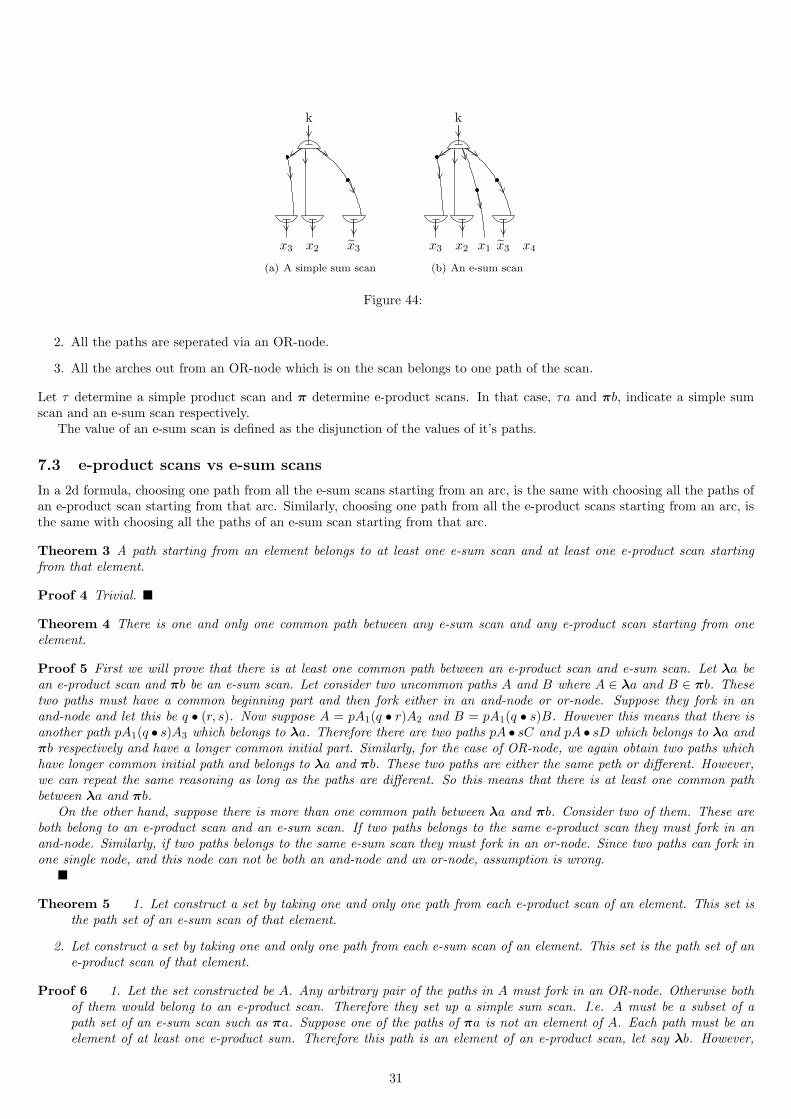
k

x3 x2 x3

(a) A simple sum scan

k

x3 x2 x4x1 x3

(b) An e-sum scan

Figure 44:

2. All the paths are seperated via an OR-node.

3. All the arches out from an OR-node which is on the scan belongs to one path of the scan.

Let τ determine a simple product scan and π determine e-product scans. In that case, τa and πb, indicate a simple sumscan and an e-sum scan respectively.

The value of an e-sum scan is defined as the disjunction of the values of it’s paths.

7.3 e-product scans vs e-sum scans

In a 2d formula, choosing one path from all the e-sum scans starting from an arc, is the same with choosing all the paths ofan e-product scan starting from that arc. Similarly, choosing one path from all the e-product scans starting from an arc, isthe same with choosing all the paths of an e-sum scan starting from that arc.

Theorem 3 A path starting from an element belongs to at least one e-sum scan and at least one e-product scan startingfrom that element.

Proof 4 Trivial. ■

Theorem 4 There is one and only one common path between any e-sum scan and any e-product scan starting from oneelement.

Proof 5 First we will prove that there is at least one common path between an e-product scan and e-sum scan. Let λa bean e-product scan and πb be an e-sum scan. Let consider two uncommon paths A and B where A ∈ λa and B ∈ πb. Thesetwo paths must have a common beginning part and then fork either in an and-node or or-node. Suppose they fork in anand-node and let this be q • (r, s). Now suppose A = pA1(q • r)A2 and B = pA1(q • s)B. However this means that there isanother path pA1(q • s)A3 which belongs to λa. Therefore there are two paths pA • sC and pA • sD which belongs to λa andπb respectively and have a longer common initial part. Similarly, for the case of OR-node, we again obtain two paths whichhave longer common initial path and belongs to λa and πb. These two paths are either the same peth or different. However,we can repeat the same reasoning as long as the paths are different. So this means that there is at least one common pathbetween λa and πb.

On the other hand, suppose there is more than one common path between λa and πb. Consider two of them. These areboth belong to an e-product scan and an e-sum scan. If two paths belongs to the same e-product scan they must fork in anand-node. Similarly, if two paths belongs to the same e-sum scan they must fork in an or-node. Since two paths can fork inone single node, and this node can not be both an and-node and an or-node, assumption is wrong.

■

Theorem 5 1. Let construct a set by taking one and only one path from each e-product scan of an element. This set isthe path set of an e-sum scan of that element.

2. Let construct a set by taking one and only one path from each e-sum scan of an element. This set is the path set of ane-product scan of that element.

Proof 6 1. Let the set constructed be A. Any arbitrary pair of the paths in A must fork in an OR-node. Otherwise bothof them would belong to an e-product scan. Therefore they set up a simple sum scan. I.e. A must be a subset of apath set of an e-sum scan such as πa. Suppose one of the paths of πa is not an element of A. Each path must be anelement of at least one e-product sum. Therefore this path is an element of an e-product scan, let say λb. However,

31

there is also a path in A which is also an element of λb since A includes a path from every e-product scan. This is notpossible because then there would be two common paths between λb and πa which contradics with the previous theorem.. Therefore, there can not be no path of πa which is not in A. This means that A is the path set of an e-sum scan.

2. Similar to the previous item.■

We have postulated that the value of an arc is the disjunction of the values of it’s e-product scan. We can do the samefor e-sum scans also.

Postulate 2 The value of an arc in any formula is equal to the conjunction of the values of all the e-sum scans startingfrom that arc.

32

Part III

Tautological properties

33

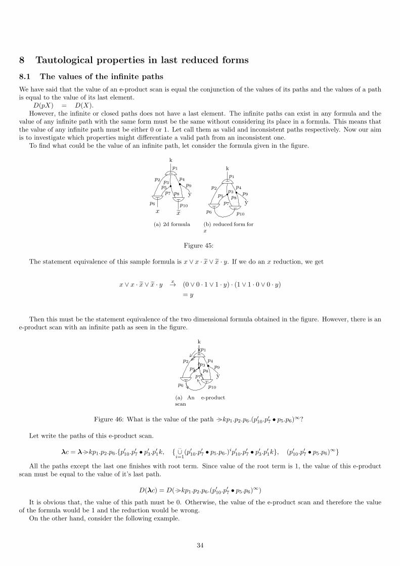
8 Tautological properties in last reduced forms

8.1 The values of the infinite paths

We have said that the value of an e-product scan is equal the conjunction of the values of its paths and the values of a pathis equal to the value of its last element.

D(pX) = D(X).However, the infinite or closed paths does not have a last element. The infinite paths can exist in any formula and the

value of any infinite path with the same form must be the same without considering its place in a formula. This means thatthe value of any infinite path must be either 0 or 1. Let call them as valid and inconsistent paths respectively. Now our aimis to investigate which properties might differentiate a valid path from an inconsistent one.

To find what could be the value of an infinite path, let consider the formula given in the figure.

k

p5

y

xx

p7

p9p3

p2

p1

p4

p8

p6 p10

(a) 2d formula

k

p5

y

p9

p2

p1

p4

p6 p10

p7p8

p3

(b) reduced form forx

Figure 45:

The statement equivalence of this sample formula is x ∨ x · x ∨ x · y. If we do an x reduction, we get

x ∨ x · x ∨ x · y x→ (0 ∨ 0 · 1 ∨ 1 · y) · (1 ∨ 1 · 0 ∨ 0 · y)= y

Then this must be the statement equivalence of the two dimensional formula obtained in the figure. However, there is ane-product scan with an infinite path as seen in the figure.

k

p5

y

p9

p2

p1

p4

p6 p10

p7p8

p3

(a) An e-productscan

Figure 46: What is the value of the path −>kp1.p2.p6.(p′10.p

′7 • p5.p6)∞?

Let write the paths of this e-product scan.

λc = λ−>kp1.p2.p6.{p′10.p′7 • p′3.p′1k, {..∪i=1

(p′10.p′7 • p5.p6.)ip′10.p′7 • p′3.p′1k}, (p′10.p

′7 • p5.p6)∞}

All the paths except the last one finishes with root term. Since value of the root term is 1, the value of this e-productscan must be equal to the value of it’s last path.

D(λc) = D(−>kp1.p2.p6.(p′10.p

′7 • p5.p6)∞)

It is obvious that, the value of this path must be 0. Otherwise, the value of the e-product scan and therefore the valueof the formula would be 1 and the reduction would be wrong.

On the other hand, consider the following example.

34

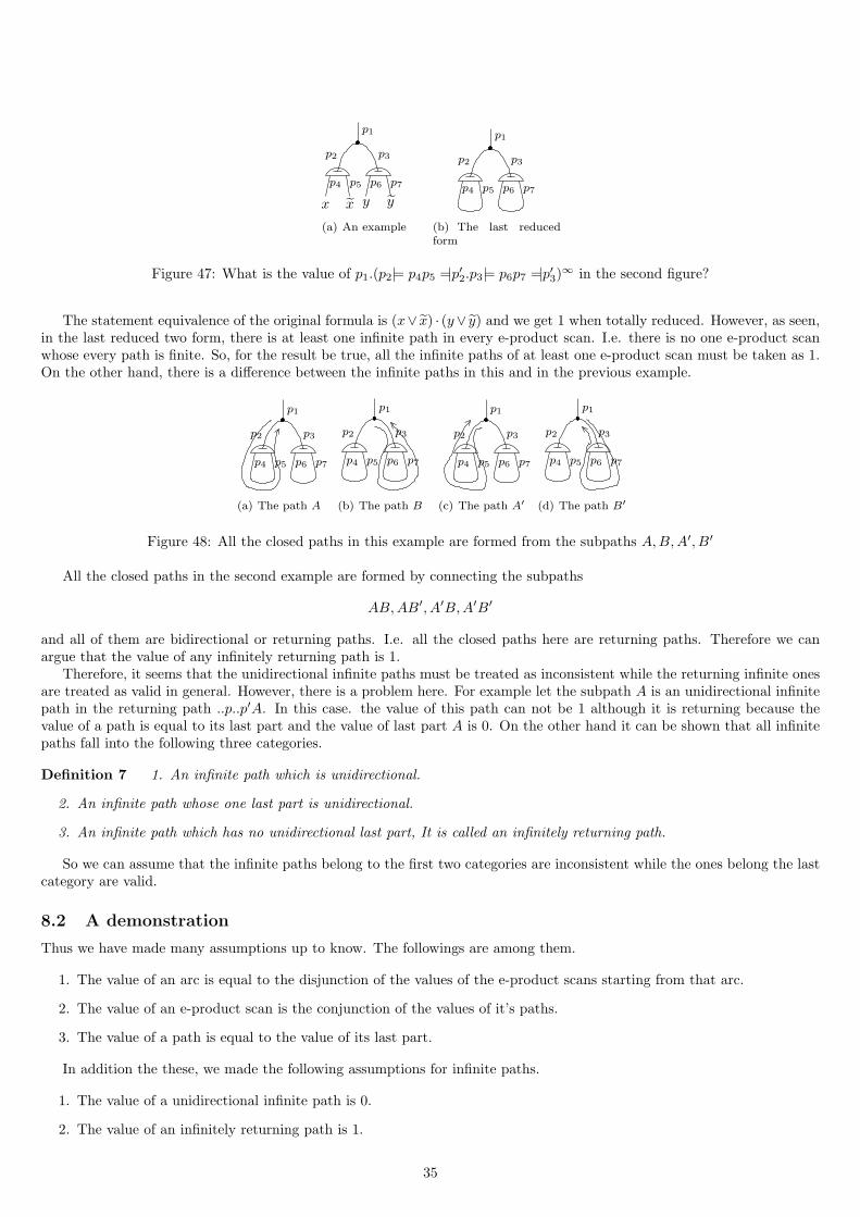
p4 p5 p6 p7

p2 p3

p1

x yx y

(a) An example

p4 p5 p6 p7

p2 p3

p1

(b) The last reducedform

Figure 47: What is the value of p1.(p2|= p4p5 =|p′2.p3|= p6p7 =|p′3)∞ in the second figure?

The statement equivalence of the original formula is (x∨ x) · (y∨ y) and we get 1 when totally reduced. However, as seen,in the last reduced two form, there is at least one infinite path in every e-product scan. I.e. there is no one e-product scanwhose every path is finite. So, for the result be true, all the infinite paths of at least one e-product scan must be taken as 1.On the other hand, there is a difference between the infinite paths in this and in the previous example.

p4 p5 p6 p7

p2 p3

p1

(a) The path A

p4 p5 p6 p7

p2 p3

p1

(b) The path B

p4 p5 p6 p7

p2 p3

p1

(c) The path A′

p4 p5 p6 p7

p2 p3

p1

(d) The path B′

Figure 48: All the closed paths in this example are formed from the subpaths A,B,A′, B′

All the closed paths in the second example are formed by connecting the subpaths

AB,AB′, A′B,A′B′

and all of them are bidirectional or returning paths. I.e. all the closed paths here are returning paths. Therefore we canargue that the value of any infinitely returning path is 1.

Therefore, it seems that the unidirectional infinite paths must be treated as inconsistent while the returning infinite onesare treated as valid in general. However, there is a problem here. For example let the subpath A is an unidirectional infinitepath in the returning path ..p..p′A. In this case. the value of this path can not be 1 although it is returning because thevalue of a path is equal to its last part and the value of last part A is 0. On the other hand it can be shown that all infinitepaths fall into the following three categories.

Definition 7 1. An infinite path which is unidirectional.

2. An infinite path whose one last part is unidirectional.

3. An infinite path which has no unidirectional last part, It is called an infinitely returning path.

So we can assume that the infinite paths belong to the first two categories are inconsistent while the ones belong the lastcategory are valid.

8.2 A demonstration

Thus we have made many assumptions up to know. The followings are among them.

1. The value of an arc is equal to the disjunction of the values of the e-product scans starting from that arc.

2. The value of an e-product scan is the conjunction of the values of it’s paths.

3. The value of a path is equal to the value of its last part.

In addition the these, we made the following assumptions for infinite paths.

1. The value of a unidirectional infinite path is 0.

2. The value of an infinitely returning path is 1.

35

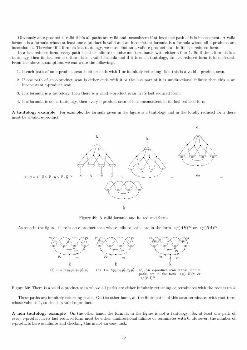
Obviously an e-product is valid if it’s all paths are valid and inconsistent if at least one path of it is inconsistent. A validformula is a formula whose at least one e-product is valid and an inconsistent formula is a formula whose all e-products areinconsistent. Therefore if a formula is a tautology, we must find an a valid e-product scan in its last reduced form.

In a last reduced form, every path is either infinite or finite and terminates with either a 0 or 1. So if the a formula is atautology, then its last reduced formula is a valid formula and if it is not a tautology, its last reduced form is inconsistent.From the above assumptions we can write the followings.

1. If each path of an e-product scan is either ends with 1 or infinitely returning then this is a valid e-product scan.

2. If one path of an e-product scan is either ends with 0 or the last part of it is unidirectional infinite then this is aninconsistent e-product scan.

3. If a formula is a tautology, then there is a valid e-product scan in its last reduced form.

4. If a formula is not a tautology, then every e-product scan of it is inconsistent in its last reduced form.

A tautology example For example, the formula given in the figure is a tautology and in the totally reduced form theremust be a valid e-product.

x · y ∨ x · y ∨ x · y ∨ x · y ∼= xyyx

k

→

k

=

k1

k2 =

k

Figure 49: A valid formula and its reduced forms

As seen in the figure, there is an e-product scan whose infinite paths are in the form −>p(AB)∞ or −>p(BA)∞.

k

p1

p3p4

p7

p5p6

p2

(a) A = −>p1.p4.p7.p′3.p′1

k

p1

p3p4

p7

p5p6

p2

(b) B = −>p2.p6.p′7.p′5.p

′2

k

p1

p3p4

p7

p5p6

p2

(c) An e-product scan whose infinitepaths are in the form −>p(AB)∞ or−>p(BA)∞

Figure 50: There is a valid e-product scan whose all paths are either infinitely returning or terminates with the root term k

These paths are infinitely returning paths. On the other hand, all the finite paths of this scan terminates with root termwhose value is 1, so this is a valid e-product.

A non tautology example On the other hand, the formula in the figure is not a tautology. So, at least one path ofevery e-product in its last reduced form must be either unidirectional infinite or terminates with 0. However, the number ofe-products here is infinite and checking this is not an easy task.

36

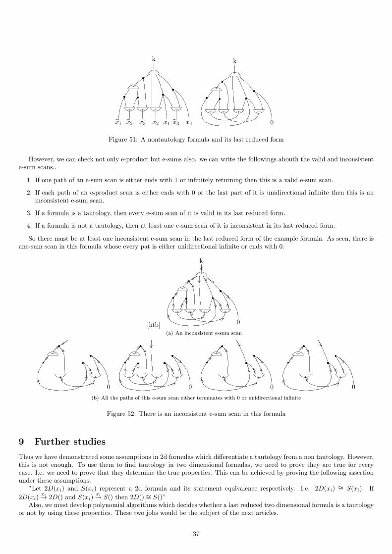
k

x2 x3 x2 x4x1 x3x1

k

0

Figure 51: A nontautology formula and its last reduced form

However, we can check not only e-product but e-sums also. we can write the followings abouth the valid and inconsistente-sum scans..

1. If one path of an e-sum scan is either ends with 1 or infinitely returning then this is a valid e-sum scan.

2. If each path of an e-product scan is either ends with 0 or the last part of it is unidirectional infinite then this is aninconsistent e-sum scan.

3. If a formula is a tautology, then every e-sum scan of it is valid in its last reduced form.

4. If a formula is not a tautology, then at least one e-sum scan of it is inconsistent in its last reduced form.

So there must be at least one inconsistent e-sum scan in the last reduced form of the example formula. As seen, there isane-sum scan in this formula whose every pat is either unidirectional infinite or ends with 0.

[htb]

k

0

(a) An inconsistent e-sum scan

0 0 0 0

(b) All the paths of this e-sum scan either terminates with 0 or unidirectional infinite

Figure 52: There is an inconsistent e-sum scan in this formula

9 Further studies

Thus we have demonstrated some assumptions in 2d formulas which differentiate a tautology from a non tautology. However,this is not enough. To use them to find tautology in two dimensional formulas, we need to prove they are true for everycase. I.e. we need to prove that they determine the true properties. This can be achieved by proving the following assertionunder these assumptions.

”Let 2D(xi) and S(xi) represent a 2d formula and its statement equivalence respectively. I.e. 2D(xi) ∼= S(xi). If

2D(xi)xi→ 2D() and S(xi)

xi→ S() then 2D() ∼= S()”Also, we must develop polynomial algorithms which decides whether a last reduced two dimensional formula is a tautology

or not by using these properties. These two jobs would be the subject of the next articles.

37

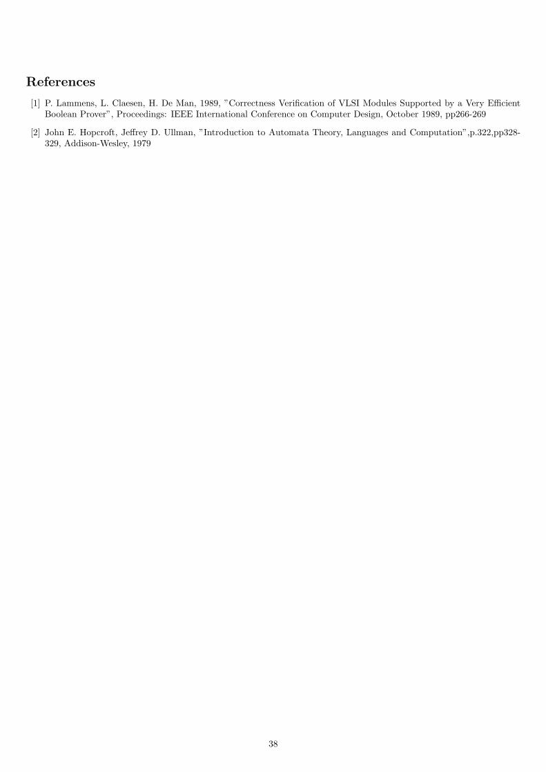
References

[1] P. Lammens, L. Claesen, H. De Man, 1989, ”Correctness Verification of VLSI Modules Supported by a Very EfficientBoolean Prover”, Proceedings: IEEE International Conference on Computer Design, October 1989, pp266-269

[2] John E. Hopcroft, Jeffrey D. Ullman, ”Introduction to Automata Theory, Languages and Computation”,p.322,pp328-329, Addison-Wesley, 1979

38