Embed Size (px)
Citation preview

University of Adelaide
VISUALIZING OPTIMIZER
By
NISARG PATEL - a1143747
Supervised By
Brad Alexander
A thesis submitted in partial fulfillment for the
degree of Master of Computer Science
in the
Department of Computer Science
June 2008

Declaration of Plagiarism
I, Nisarg Patel, declare that this thesis titled, ‘Visualizing Optimizer’ and the work pre-
sented in it are my own. Where I have consulted the published work of others, this is
always clearly attributed and any error in that is totally unintentional.
I have read University’s policies on plagiarism before submission of my work.
Signed:
Date:
i

“Seeing is Believing”

Abstract
Code optimizers transform code from one form to another more efficient one. Most
optimizers are quite complicated in their design, as a result their internal behavior is
always difficult to monitor and trace. This project is based around an optimizer, BMF
optimizer written in Stratego, which is simple in design, specifically designed to be easy
to debug, analyze and trace. Due to its small and simple transformation steps the number
of transformations is quite higher than other optimizers. This is a bottleneck in evolution
of optimizer, because high number of transformations creates obscurity. The main aim
of this project is to trace the execution, performance and intermediate transformed code.
For that, optimizer’s generated list of ASTs has to be converted it into X3D abstract
syntax and write pretty printer to create concrete syntax which can display the trace in
graphical manner. The aim of the project was to built a 3D model of trace which is, easy
to understand, easy to navigate and should help in future development of the optimizer.

Acknowledgements
This project would not have come to existence without support from many people.
First of all I sincerely thank my parents for their blessings and support. Throughout my
studies they have motivated and supported me in whatever way they could and whatever
way I wanted. They have been the real source of inspiration throughout my studies.
Without the help of my supervisor Brad Alexander, I might not have finished this project
so successfully. I would like to thank him for his valuable suggestions, observations, his
help in my silly to gigantic mistakes and help with writing. I am also grateful for his
patience and support throughout the project time.
I would like to thank my close friend Aruna for her every help which always seemed liked
a little drop but now collectively have become an ocean.
Last but not the least, I would like to thank all who have directly or indirectly helped,
inspired or supported me for this work.
iv
Contents
Declaration of Plagiarism i
Abstract iii
Acknowledgements iv
List of Figures vi
1 Introduction 1
2 Stratego And Existing Optimizer 3
2.1 Rules . . . . . . . . . . . . . . . . . . . . . . . . . . . . . . . . . . . . . . 4
2.2 Strategies . . . . . . . . . . . . . . . . . . . . . . . . . . . . . . . . . . . 5
2.3 Pretty Printing . . . . . . . . . . . . . . . . . . . . . . . . . . . . . . . . 6
2.4 Optimizer And Optimization Process . . . . . . . . . . . . . . . . . . . . 6
3 Problem And Possible Solutions 8
3.1 Problem . . . . . . . . . . . . . . . . . . . . . . . . . . . . . . . . . . . . 8
3.2 Possible Solution . . . . . . . . . . . . . . . . . . . . . . . . . . . . . . . 10
4 X3D 11
4.1 Why Not Others? . . . . . . . . . . . . . . . . . . . . . . . . . . . . . . . 11
4.1.1 Adobe Flash . . . . . . . . . . . . . . . . . . . . . . . . . . . . . . 11
4.1.2 POVRAY . . . . . . . . . . . . . . . . . . . . . . . . . . . . . . . 12
4.1.3 Blender And 3Ds Max . . . . . . . . . . . . . . . . . . . . . . . . 12
4.1.4 3D PDF . . . . . . . . . . . . . . . . . . . . . . . . . . . . . . . . 12
4.1.5 SketchUp . . . . . . . . . . . . . . . . . . . . . . . . . . . . . . . 12
4.2 What Is X3D . . . . . . . . . . . . . . . . . . . . . . . . . . . . . . . . . 13
4.3 Advantages Of X3D . . . . . . . . . . . . . . . . . . . . . . . . . . . . . . 13
4.4 X3D Profiles . . . . . . . . . . . . . . . . . . . . . . . . . . . . . . . . . . 14
4.5 X3D File Structure . . . . . . . . . . . . . . . . . . . . . . . . . . . . . . 15
4.5.1 File Header . . . . . . . . . . . . . . . . . . . . . . . . . . . . . . 15
4.5.2 File Body . . . . . . . . . . . . . . . . . . . . . . . . . . . . . . . 17
4.6 X3D Nodes . . . . . . . . . . . . . . . . . . . . . . . . . . . . . . . . . . 18
v
Contents vi
4.7 Animation . . . . . . . . . . . . . . . . . . . . . . . . . . . . . . . . . . . 19
4.8 Sensor . . . . . . . . . . . . . . . . . . . . . . . . . . . . . . . . . . . . . 19
4.9 Scripts . . . . . . . . . . . . . . . . . . . . . . . . . . . . . . . . . . . . . 20
5 Preliminary Experiments 23
5.1 Ability To Draw Tree . . . . . . . . . . . . . . . . . . . . . . . . . . . . . 24
5.2 Animation . . . . . . . . . . . . . . . . . . . . . . . . . . . . . . . . . . . 25
5.3 Button Capability In X3D . . . . . . . . . . . . . . . . . . . . . . . . . . 27
5.4 Scripting For User Interactivity . . . . . . . . . . . . . . . . . . . . . . . 28
6 3D Model Generation 31
6.1 Generate List Of ASTs . . . . . . . . . . . . . . . . . . . . . . . . . . . . 32
6.2 Adding Performance Data . . . . . . . . . . . . . . . . . . . . . . . . . . 32
6.3 Generating X3D’s Syntax Definition . . . . . . . . . . . . . . . . . . . . . 33
6.3.1 Knowing X3D Syntax . . . . . . . . . . . . . . . . . . . . . . . . 33
6.3.2 Generating X3D Syntax . . . . . . . . . . . . . . . . . . . . . . . 37
6.4 From AST To X3D Abstract Syntax . . . . . . . . . . . . . . . . . . . . 39
6.4.1 Generating Viewpoints . . . . . . . . . . . . . . . . . . . . . . . . 39
6.4.2 Removing Quotes . . . . . . . . . . . . . . . . . . . . . . . . . . . 40
6.4.3 Getting Indentation For Tree . . . . . . . . . . . . . . . . . . . . 43
6.4.4 Printing Text . . . . . . . . . . . . . . . . . . . . . . . . . . . . . 43
6.4.5 Putting All Nodes Together To Form A Tree . . . . . . . . . . . . 44
6.4.6 Putting The Tree In A Group . . . . . . . . . . . . . . . . . . . . 45
6.4.7 Putting Trees At Proper Location In Scene . . . . . . . . . . . . . 46
6.4.8 Gathering All Trees . . . . . . . . . . . . . . . . . . . . . . . . . . 47
6.5 Generation of Final X3D File (Pretty Printing) . . . . . . . . . . . . . . 48
6.5.1 Printing File Header . . . . . . . . . . . . . . . . . . . . . . . . . 48
6.5.2 Printing Viewpoints . . . . . . . . . . . . . . . . . . . . . . . . . 49
6.5.3 Adding Text . . . . . . . . . . . . . . . . . . . . . . . . . . . . . . 50
6.5.4 Adding Buttons . . . . . . . . . . . . . . . . . . . . . . . . . . . . 51
6.5.5 Adding Script And Route Information . . . . . . . . . . . . . . . 52
7 Results 54
7.1 Printing Just Text . . . . . . . . . . . . . . . . . . . . . . . . . . . . . . 55
7.2 Printing Text In Tree Format . . . . . . . . . . . . . . . . . . . . . . . . 56
7.3 Adding Buttons . . . . . . . . . . . . . . . . . . . . . . . . . . . . . . . . 57
7.4 Adding Scripts . . . . . . . . . . . . . . . . . . . . . . . . . . . . . . . . 58
7.5 Adding Performance Data . . . . . . . . . . . . . . . . . . . . . . . . . . 59
7.6 Full Result . . . . . . . . . . . . . . . . . . . . . . . . . . . . . . . . . . . 60
7.7 Some Facts . . . . . . . . . . . . . . . . . . . . . . . . . . . . . . . . . . 62
8 Future Work 63
9 Conclusion 64

Contents vii
A X3D Syntax File 65
B X3D Signature File 67
C Syntax Example For Single Tree 69
D Abstract Syntax File Example 74
E Pretty Printing File 75
Bibliography 83
List of Figures
2.1 Conversion From Code To AST . . . . . . . . . . . . . . . . . . . . . . . 3
2.2 Conversion From AST To Code . . . . . . . . . . . . . . . . . . . . . . . 4
2.3 Program Transformation Example . . . . . . . . . . . . . . . . . . . . . . 7
4.1 X3D Profiles . . . . . . . . . . . . . . . . . . . . . . . . . . . . . . . . . . 14
4.2 X3D File Structure . . . . . . . . . . . . . . . . . . . . . . . . . . . . . . 16
5.1 X3D Experiment Outline . . . . . . . . . . . . . . . . . . . . . . . . . . . 23
5.2 Initial Tree Form . . . . . . . . . . . . . . . . . . . . . . . . . . . . . . . 24
5.3 Final Tree Form . . . . . . . . . . . . . . . . . . . . . . . . . . . . . . . . 25
5.4 X3D Animation Example 1 . . . . . . . . . . . . . . . . . . . . . . . . . 26
5.5 X3D Animation Example 2 . . . . . . . . . . . . . . . . . . . . . . . . . 26
5.6 X3D Button Capability . . . . . . . . . . . . . . . . . . . . . . . . . . . . 27
5.7 Example File Of Functional Script . . . . . . . . . . . . . . . . . . . . . 28
5.8 Example File Of Simple Script . . . . . . . . . . . . . . . . . . . . . . . . 29
6.1 Milestones To Generate Final 3D Model . . . . . . . . . . . . . . . . . . 31
6.2 Created First Graphics File To Know X3D Syntax . . . . . . . . . . . . . 34
6.3 Created Second Graphics File To Know X3D Syntax . . . . . . . . . . . 34
6.4 Text Before Removing Extra Quotes . . . . . . . . . . . . . . . . . . . . 41
6.5 Text After Removing Extra Quotes . . . . . . . . . . . . . . . . . . . . . 42
7.1 Result - Printing Text In X3D . . . . . . . . . . . . . . . . . . . . . . . . 55
7.2 Result - Tree Format In X3D . . . . . . . . . . . . . . . . . . . . . . . . 56
7.3 Result - Buttons In X3D . . . . . . . . . . . . . . . . . . . . . . . . . . . 57
7.4 Result - Scripts In X3D . . . . . . . . . . . . . . . . . . . . . . . . . . . 58
7.5 Result - Performance Data In X3D . . . . . . . . . . . . . . . . . . . . . 59
7.6 Full Result . . . . . . . . . . . . . . . . . . . . . . . . . . . . . . . . . . . 60
7.7 Full Result In Different View . . . . . . . . . . . . . . . . . . . . . . . . . 60
7.8 Result In Flattened View . . . . . . . . . . . . . . . . . . . . . . . . . . . 61
7.9 Facts . . . . . . . . . . . . . . . . . . . . . . . . . . . . . . . . . . . . . . 62
viii
Chapter 1
Introduction
Compiler optimization techniques are, as name suggests, embedded in compiler. Compil-
ers apply appropriate optimization techniques, as it goes on compiling the given code, to
increase code’s performance. Because of this programmers do not have to worry about low
level optimization. As a result, compiler optimizers have to be on their best to increase
performance.
This project takes an existing BMF (Bird-Meertens Formalism) optimizer. BMF is a func-
tional programming model consisting purely of scalar and list functions and higher order
functions1 to glue them [7]. BMF allows one to take an initial program and transform it
into one that is computationally equivalent, but more efficient. This optimizer is written
in Stratego, which is a language for program transformation based on the paradigm of
programmable rewriting strategies [27]. It is a rule based optimizer which has set of rules.
While optimizing, a rule recognizes a sub term (part of code) to be transformed by pattern
matching and replaces that sub term with pattern instance. Most rules in the optimizer
simply rewrite from a source to target expression. These rules can be applied in various
ways or in various sequences, which can be controlled by programmable strategies. The
Stratego language and basic working of optimizer are explained in Chapter 2.
Many rules, of this optimizer’s rule set, perform very trivial and small task. This makes
the amount of change in every transformation very little and mainly localized but when
many of this small transformations come together, it creates global impact. Thus, it is
apparent that optimizer will have to make many local and small transformations in order
to optimize even a code with medium complexity. However, when the code is very large
1Higher order functions are those which take other BMF expressions as arguments and hence havechildren in their parse tree.
1

Chapter 1. Introduction 2
and complex it takes hundreds to thousands of transformation, which makes tracking of
trace and performance difficult. Moreover, unless and until the performance of individual
rules and their internal behavior for all the transformations are checked and assed, it
is hard to validate and access the optimizer. In addition to that, for optimization, in
this optimizer, rules can be applied in very large number of possible permutation and
combination using different strategies. So it becomes difficult to compare that which
combination of rules give better performance, if there is no easy mechanism to compare.
This problem, along with the example, and its possible solutions are depicted in chapter
3.
One way to solve this problem is to ’see’ every transformation with as much of detail as
possible. We have solved this problem by displaying the initial code, final code and all
intermediate transformed code, in its abstract syntax tree format, in 3D environment.
We have also made it possible to navigate through the long list of transformed codes by
adding navigation functionality. To create this 3D model we have used X3D, which is an
XML based 3d graphics rendering tool. In chapter 4, X3D has been explained in detail,
as well as features of X3D and other possible graphics rendering tools are compared.
While selecting X3D as final choice we had to run some preliminary experiments by which
we came to know a lot about X3D. These experiments and their findings are explained
in chapter 5.
How we have approached the solution, what were the mile stones, what problems we have
faced, what are our findings, and other details are explained in chapter 6. The results of
project is shown in chapter7, while some future work is explained in chapter 8.
Chapter 2
Stratego And Existing Optimizer
As given in [1], Stratego is a language specifically designed for program transformation.
The language provides rewrite rules for the definition of basic transformations, and pro-
grammable strategies for building complex transformations that control the application
of rules. Complex program transformation can be achieved by number of consecutive
modifications in a given code.
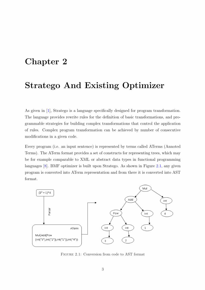
Every program (i.e. an input sentence) is represented by terms called ATerms (Annoted
Terms). The ATerm format provides a set of constructs for representing trees, which may
be for example comparable to XML or abstract data types in functional programming
languages [8]. BMF optimizer is built upon Stratego. As shown in Figure 2.1, any given
program is converted into ATerm representation and from there it is converted into AST
format.
Figure 2.1: Conversion from code to AST format
3
Chapter 2. Stratego And Existing Optimizer 4
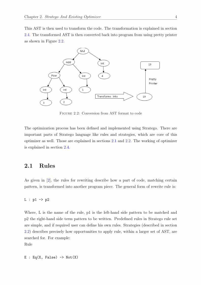
This AST is then used to transform the code. The transformation is explained in section
2.4. The transformed AST is then converted back into program from using pretty printer
as shown in Figure 2.2.
Figure 2.2: Conversion from AST format to code
The optimization process has been defined and implemented using Stratego. There are
important parts of Stratego language like rules and strategies, which are core of this
optimizer as well. Those are explained in sections 2.1 and 2.2. The working of optimizer
is explained in section 2.4.
2.1 Rules
As given in [2], the rules for rewriting describe how a part of code, matching certain
pattern, is transformed into another program piece. The general form of rewrite rule is:
L : p1 -> p2
Where, L is the name of the rule, p1 is the left-hand side pattern to be matched and
p2 the right-hand side term pattern to be written. Predefined rules in Stratego rule set
are simple, and if required user can define his own rules. Strategies (described in section
2.2) describes precisely how opportunities to apply rule, within a larger set of AST, are
searched for. For example:
Rule
E : Eq(X, False) -> Not(X)
Chapter 2. Stratego And Existing Optimizer 5
will transform the term
Eq(Atom("q"),False) into Not(Atom("q")),
because X has been bound with Atom(�q�).
2.2 Strategies
It is clear from above example that, a rule defines transformation, which is a heart of
optimization. As given in [18], most other systems embed rewriting rules in recursive
definition to traverse the AST. This embedding prevents the rewriting part of the trans-
formation from being reused in a different traversal strategy leading to much longer code.
Moreover, this method not sufficient for well program optimization. Because this may
lead the optimization process into non-terminating state if one rule is in inverse of the
other [3].
In addition to that, it is also possible that applying different rules in different sequence
may give different results. Thus to control that, rules should be applied strategically. To
solve this problem, strategies are used in Stratego, which combines one or more rules and
applies them in predefined traversal sequence throughout the tree. Strategies define how
rules are applied. Strategies make the rule look for left hand side pattern in given term
and when the match is found, it will rewrite/transform it to right hand side pattern. As
given in [2], a strategy definition has the form:
F = S
Where, F is name of the strategy and S is the strategy expression. Strategy expressions
can combine one or more transformations (rules and/or transformations) into a new
transformation.
For example, s1 <+ s2 tries to apply rule s1 first and if application of s1 fails then it tries
to apply rule s2. This strategy also helps when the rules are mutually exclusive, because
even if one rule fails the other can succeed.
Bottom-up traversal strategy makes it possible to traverse the whole tree starting from
bottom. In other words, it first visits the subterms of the subject term, recursively
transforming its subterms, and then tries to transform the subject term. This strategy is
defined as below.
Chapter 2. Stratego And Existing Optimizer 6
bottomup(s) = all(bottomup(s)); s
Now for example, strategy
bottomup(try(L)) applied to term T
will attempt to apply rule L to each node of the AST from bottom up. It is worth noting
that, this attempt will fail at most nodes in the tree, because the node does not match
the left hand side pattern of the rule.
2.3 Pretty Printing
We have used the ast2text tool to pretty print text [20]. This tool prints the abstract
syntax tree into plain text. The utility transforms an abstract syntax tree according to
formatting rules contained in pretty-print tables. The result of ast2text is an ASCII text
file. The tool is a convenience composition of ast2abox1 and abox2text2 tools. The pretty
printing format we have used in explained in section 6.5 as well as whole pretty printing
file is attached in appendix 4. In this tool -p option informs the pretty printer where the
formatting rules are stored. -i and -o informs the pretty printer from where to fetch input
file and where to store the output file respectively.
2.4 Optimizer And Optimization Process
BMF optimize creates an intermediate form to allow for easier optimization. The opti-
mizer is written in stratego. It consists of several small modules of very simple rewrite
rules that are repeatedly combined and applied to code using a small set of strategies
until the code reaches a form that we have previously seen.
It should be noted that, the main aim of the project is to create a 3D model of the long
trace. These traces are treated in the whole project as just a list of trees. What any
trace or program means is irrelevant to our problem. These programs and their trace
1ast2abox pretty prints an abstract syntax tree to the Box layout formalism. The result of ast2aboxis a Box term which describes the intended format.
2abox2text formats a Box term to plain text. The result of abox2text is plain text according to theformatting defined in a Box
Chapter 2. Stratego And Existing Optimizer 7
can be understood by people involved in development of the optimizer. So there will be
minimum level of explanation of content like the optimizer code and stratego code. We
have put Stratego programs and their traces at few places to explain its complexity, to
give some background information, to manage consistency and for clearer understanding
of our work.
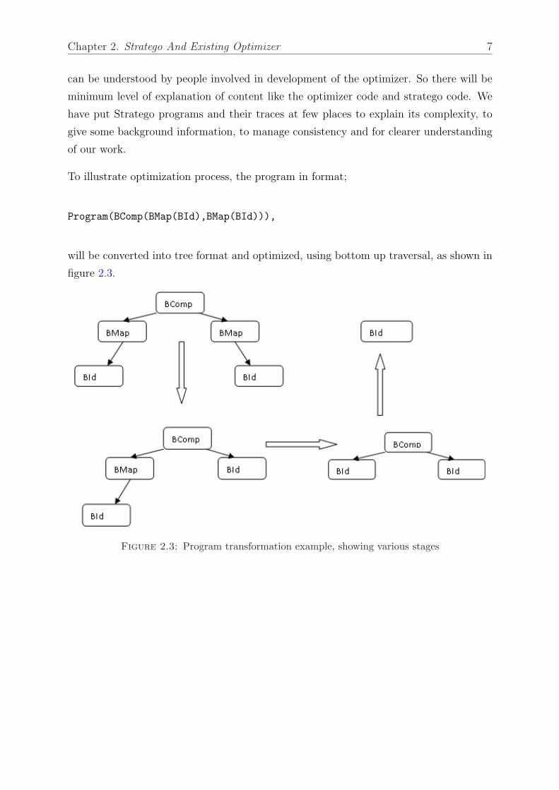
To illustrate optimization process, the program in format;
Program(BComp(BMap(BId),BMap(BId))),
will be converted into tree format and optimized, using bottom up traversal, as shown in
figure 2.3.
Figure 2.3: Program transformation example, showing various stages

Chapter 3
Problem And Possible Solutions
3.1 Problem
For tracing purpose the optimizer is able to provide some data. This data is merely a
text dump, which is hard to process and understand. The example program shown in
previous chapter,
Program(BComp(BMap(BId),BMap(BId))),
is one of the very trivial programs and still it takes 3 transformations to optimize the
code fully. Now the existing optimizer can give some data to trace the execution which
would be as follows.
Program(BTrace([BComp(BMap(BId),BMap(BId)),BComp(BId,BMap(BId)),
BComp(BId,BId),BId]))
This trace is just merely a text dump. It contains data but no information. But still it
is easy to fetch required information from above text dump then what is the problem?
For the simplest program like above, it takes 3 transformations to optimize. When the
code gets larger, the number of transformations increases exponentially. Because code’s
smaller parts need transformation, and combined transformed components needs further
transformation. This makes the understanding of trace more complicated.
For instance a little bit bigger code like shown below increases the number of transfor-
mations to 11.
8
Chapter 3. Problem And Possible Solutions 9
Program(BComp(BComp(BComp(BMap(BComp(BOp(BIndex),BAlltup([BAddr("2","1"),
BAddr("2","2")]))),BOp(BDistl)),BAlltup([BId,BComp(BOp(BIota),
BComp(BOp(BLength),BId))])),BId))
This code’s trace will be as follows:
Program(BTrace([BComp(BComp(BComp(BMap(BComp(BOp(BIndex),BAlltup([BAddr("2","1")
,BAddr("2","2")]))),BOp(BDistl)),BAlltup([BId,BComp(BOp(BIota),
BComp(BOp(BLength),BId))])),BId), ... ... ,BComp(BComp(BOp(BSelect),
BAlltup([BId,BComp(BOp(BIota),BOp(BLength))])),BId),BComp(BId,BId),BId]))
Now for instance if the code remains of the same size, but complexity increases, like the
code shown below, then it becomes more tough and number of transformations fly to 120.
Program(BComp(BComp(BComp(BMap(BComp(BComp(BComp(BMap(BComp(BOp(BPlus),
BAlltup([BAddr("2","2"),BCon(BInt("2"))]))),BOp(BDistl)),
BAlltup([BId,BAddr("2","2")])),BId)),BOp(BDistl)),BAlltup([BId,BId])),BId))
These codes are still basic ones. This shows that in this optimizer it’s not too tough
for number of transformations to fly in hundreds and in certain cases up to thousands.
This makes it impossible to trace the optimization process and thus the whole process
becomes obscure. This situation is not good for optimizer’s enhancement. If one can not
see which rules are not working well or giving adverse effect on performance, it’s hard to
manage them it’s even harder to manage the strategies, which handles these rules and as
a result whole process gets unmanageable. It is worth noting that still these rules can be
verified on smaller and individual basis but it is not sufficient.
The problem goes out of control when two different optimization processes on the same
code, using different strategies, has to be compared. Because one can not know at which
point one optimizer got ahead, in terms of performance, of the other or vice versa and
have to only rely on the end result.
Another case can be when two different versions of optimizers have to be compared for
performance. In that case many programs will have to be run in both version of optimizer
and every single rule has to be evaluated for performance. In that case it is definitely not
compared to sit with long list of trace and keep comparing it.
In simple words, the problem is with tracking every single transformation in optimization
process with as much detail as possible, which is simply must.
Chapter 3. Problem And Possible Solutions 10
3.2 Possible Solution
A solution to this might be to arrange the text dump produced by optimizer in appropriate
way so that it can show the desired information. E.g. in a spreadsheet nicely arrange data
which shows existing tree in text format, performance figure, name of applied rule, etc.
But this solution requires user to imagine how the program structure is. This becomes
complicated when programs, and thus their representing trees, are very large or complex.
In other words this solution is just nicely arranging the text dump.
There is another approach, which we have taken; to display all needed information graph-
ically. The whole code along with every transformation can be shown graphically in ab-
stract syntax tree format. In this solution, it can be made possible to navigate through
all the transformations. The performance data can be shown along with each and every
tree. This removes the need of imagining anything. Two different version of optimizer’s
performance can be compared easily. It can also be actually seen whether any rule have
broken the code or not.

Chapter 4
X3D
We had some requirements in mind on basis of which we wanted to choose the 3d modeling
tool. These requirements were as follows. A tool, including its viewer should be, if
possible, free, should have good 3d modeling capability so that 3d models should look
reasonably good, should provide animation so that 3d model should not be just an image
and it should provide user interactivity so that an interaction can be made with trace.
4.1 Why Not Others?
4.1.1 Adobe Flash
This tool is very famous for creating 3d animation, user interactive animation and internet
applications [10]. It can be smoothly used in mobile devices as well [9]. Its action script
provides very flexible programmable action event management. Although, flash’s action
scripts are not a standard, it can be generated using some free tools [12].
It’s one of the down side is that its official development tool, Flash CS3 Professional, is
not free (at the time of research its cost was USD 600+) [11]. Moreover, it is not an
open standard. So for full features its official development tool has to be used [13] and
cannot be generated from third party software [26]. Due to this disadvantage it could not
be created directly from a Stratego program and was not suitable for project. In simple
words, its action script can be generated from third party software but not the actual
drawing (tree in our case),which is animated using action script that has to be animated.
11
Chapter 4. X3D 12
4.1.2 POVRAY
POVRAY (Persistence of Vision Raytracer) is freeware for developing 3d graphics. It
uses programming language style to generate 3d model (little bit similar to X3D and C).
So models can be generated directly from Stratego program. Its rendering capability is
very good. It supports animation. But it’s down side is that it does not support user
interactivity [14]. Thus it cannot allow user to take control and go back and forth in
long drawing of ASTs. This can restrict user from skipping some transformation while
navigating through a 3D model of any long trace. This tool can generate time based
animation (like movies), but it is not user interaction. After generating few models in
this tool due to lack of interactivity it was not chosen.
4.1.3 Blender And 3Ds Max
These are well known applications to generate 3d models. They have very advance an-
imation features. They can create stunning 3d models. But, as given in [16] and [15],
they are not an open standard files, which can be created from any third party system.
This can prevent generating their code from Stratego program. Moreover, they does not
have user interactivity feature, which will prevent from interacting with trace.
4.1.4 3D PDF
This is a new tool created by Adobe. As given in [17], it can create 3d world which can
be exported in highly accessible pdf format. It provides user interactivity. It provides
animation. Its viewers are free. But again its development tool is not free and it is not
an open standard.
4.1.5 SketchUp
This is a tool from Google. It provides very good modeling. It does have ability to
animate the camera. Fully featured development tool is not free. The free tool is good
enough but not as good as the paid one. It is not an open standard [28]. It does not have
user interactivity. It can include/export in various file formats but then sketchup doesn’t
remain the 3d tool in question.
Chapter 4. X3D 13
4.2 What Is X3D
As given in [5], X3D, which stands for ”Extensible 3D”, is a new, still under development,
open standard for 3D content on the internet. It is not a language but a standard. It
is developed by Web3d consortium and is successor of famous Virtual Reality Modeling
Language (VRML). X3D is intended to replace/extend the existing VRML97 standard
to display 3D interactive graphics on the web. X3D is a file format specification with
requirements on how a file is to be displayed. It is an ISO standard for 3D graphics. X3D
is more flexible than its predecessors because its files are encoded in XML, which can be
extended.
X3D has modular architecture which allows layered profiles. Profiles are used for incre-
mental implementation of standard. As claimed in [4], these profiles can be arranged
at different layers and thus can share services or interchange data among them. For
instance a profile at higher layered can access all functionality, known as components,
which a lower layered profile may not be able to. E.g. sound functionality cannot be used
by any profile which is at lower level then immersive. This enables users to use/access
only required functionalities and can make the application lighter, smoother and faster.
These profiles can increase functionality for graphical world and can enhance interactivity
as well. More about profiles is explained in section 4.4.
From [5], the X3D architecture is divided in components as well. There are 28 basic
components defined. It is also possible to modify a profile by adding different desired
components. This also makes the application lighter as it does not need higher profile
just because of 2-3 components. In addition to that, new components can also be added
to launch new features, e.g. streaming.
4.3 Advantages Of X3D
Although X3D neither has plenty of books written on it nor has wide web based support or
explanation, we decided to use it due to its features. The main reason to use X3D is that
X3D can create sophisticated 3d model simply. It has got flexibility and accessibility. It
does not need licensed software to view and to create the graphics file [5]. X3D combines
both geometry and runtime behavior into a single XML file [19]. This XML files can be
created using purpose built X3D authoring tools (e.g. X3D edit), text editors (WordPad,
text wrangler) or exported from third party applications (Stratego program in our case).
Chapter 4. X3D 14
This was also very important feature to pick X3D. Some features of X3D like zoom in/out,
simple user interactivity, 3d modeling, and possibility to fly around in 3d world was also
considered important for this project and its future development (like interactive graph
display).
These created X3D files can be displayed in a native X3D browser, which are sometime
available for free, or a web browser that has an X3D plug-in. Moreover the component
based structure helps to download and play files faster over the web [4]. By specifying a
lower profile along with some extra needed components, can make profile compatible for
most browsers.
4.4 X3D Profiles
As stated earlier, X3D profiles provide incremental implementation of standard. As
given in [4] and [5], X3D has 4 basic profiles defined in it. Each profile is targeted
for functionality that is commonly used. Because of these profiles even X3D browsers
or web browsers can provide immediate support, rather than trying to implement big
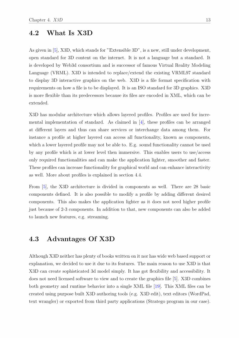
specification at once. These profiles are shown in figure 4.1.
Figure 4.1: X3D profiles with example of type of ndes available at each profile
Interchange is the most basic profile, which helps to communicate between applications.
It supports very basic graphics features like texturing, geometry, basic lighting. This
profile makes it possible to simply draw basic 3d objects.

Chapter 4. X3D 15
The second basic profile is interactive. This helps to interact with the basic 3d envi-
ronment which was created by interchange profile. This provides timing facility and
additional lighting facilities like point light and sensor light. Additional to interchange
profile this profile provides various sensor nodes which help user to navigate and interact.
As claimed in [4], immersive is the most used profile. It provides full 3d graphics and user
interaction. It also provides some of the advance features like fog, collision of objects,
scripting and audio support. In our project we have used this profile because it fulfills the
requirement of scripting ability, touch sensor ability and ability to draw different shapes.
Full is the rarely used profile unless specifically needed. It includes all the defined nodes
in X3D. It includes NURBS1, H-Anim (Human animation), and geospatial components.
X3D have 2 additional profiles defined which also provide specific solution. MPEG-4
Interactive is a small footprint version of the Interactive profile designed for broadcast,
handheld devices and mobile phones. Another one is CDF (CAD Distillation Format),
which is in, as claimed in [6], development phase to enable translation of CAD data to
an open format for publishing and interactive media. These two profiles are still under
development.
4.5 X3D File Structure
X3D files use .x3d format for XML based encoding or .x3dv for classical VRML based
encoding. As given in [4], X3D uses scene graph technique for rendering and animation
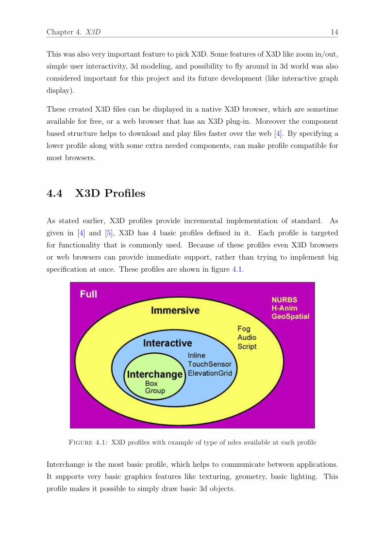
purpose. This graph structure remains consistent in both types of encodings. The general
file structure is shown in figure 4.2. I have used our own created X3D file as an example,
to show these different sections.
4.5.1 File Header
X3D file header contains no graphical information. It just contains some basic X3D scene
setup information. The file header contains XML and X3D headers, profiles, optional
components and meta information. The first information is XML information which
identifies the file as XML encoded file. The XML encoding matches general XML header
requirement, starting with the <?xml?> declaration.
1 NURBS (non-uniform, rational B-spline) is a mathematical model commonly used in computergraphics for generating and representing curves and surfaces.
Chapter 4. X3D 16
Figure 4.2: The basic X3D file structure
<?xml version="1.0" encoding="UTF-8"?>
As shown above, it also includes version number and encoding. X3D files use (universal
text format) UTF-8 encoding to support almost all electronic alphabets.
After that there is X3D header statement which identifies the XML file to be an X3D
file. As shown below, The Document Type Definition (DTD), which is indicated by
DOCTYPE statement. Those help to validate the correctness of .X3D file.
<!DOCTYPE X3D PUBLIC "http://www.web3d.org/specifications/x3d-3.1.dtd" "file:///www.web3d.org/TaskGroups/x3d/translation/x3d-3.1.dtd">
Following that there is a declaration of X3D’s version number (version 3.0 and 3.1 are
only allowed) profile used in model and an XML Schema reference. This part is also
important because as per profile’s declaration the components and features can be used.
An example is shown below. Importance of profile is explained in section 4.4.
Chapter 4. X3D 17
<X3D profile="Immersive" version="3.1"
xmlns:xsd="http://www.w3.org/2001/XMLSchema-instance"
xsd:noNamespaceSchemaLocation=
"http://www.web3d.org/specifications/x3d-3.1.xsd">
Following that there is optional filed to add extra components to previously declared
profile as well as to add meta information. Meta information is useful to provide copyright,
author, other information. As it uses name-value string pairs (name of the item and
corresponding content), it can contain mostly any kind of information. Meta data can be
very beneficial as a part of project because it can store the values of different optimizer
version number or trial run number etc. Its example is as follows:
<head>
<meta content="*enter FileName here*" name="title"/>
<meta content="*enter description here,
short-sentence summaries preferred*" name="description"/>
<meta content="*enter name of author here*" name="creator"/>
<!-- SIMILARLY OTHER INFORMATION -->
</head>
4.5.2 File Body
Following the header of X3D file its actual body comes starting with <Scene> tag. The
creation of a scene in X3D is done through the definition and organization of the scene
graph. As shown below, the scene graph is a hierarchical structure that is made up of
nodes. These nodes act as parents and children. The Scene node is the root node, and
is the parent node of any scene (3D model). The Scene node’s children define all of the
items in a scene and their attributes. The nodes define objects such as shapes, sensors,
scripts, transformations, lightings, groups, etc
<Scene>
<!--Scene graph nodes are added here -->
<DirectionalLight ambientIntensity="0" color="1 1 1" direction="0 0 -1"
global="true" intensity="1" on="true"/>
<Viewpoint centerOfRotation="0 0 0" orientation="0 0 0" position="0 0 10"/>
<Shape>

Chapter 4. X3D 18
... ... ...
</Shape>
</Scene>
In above example, directional light gives light in the scene with defined intensity, color and
direction. Viewpoint setups a camera location by giving center of rotation, orientation
and position. As .x3d files use XML encoding, all scenes must be well formed, which
includes properly opened, closed, single or double quoted attributes, singleton tags, etc.
Each node in the X3D body have one or more fields which store the require data for that
node. E.g. a cone node can have fields like solid, bottom radius, height, side, bottom, etc.
which looks like below. Shape nodes can also contain other information like, appearance,
material information, transparency, etc.
<Shape>
<Appearance>
<Material emissiveColor="0 1 0"/>
</Appearance>
<Cone DEF=’the-cone’ bottomRadius="3.5" height="1.5" solid="false"
bottom="false"/>
</Shape>
4.6 X3D Nodes
As given in [19], X3D have many different kinds of nodes to provide different kind of
functionality. Although they can be basically grouped as follows:
� Coordinate Nodes (like: Coordinate, Transform)
� Geometry Nodes (like: IndexedFaceSet, IndexedLineSet, IndexedPointSet)
� Grouping Nodes (like: Anchor, Group, Inline, Transform)
� Light Nodes (like: Directional Light)
� Material Nodes (like: Material)
� Shape Nodes (like: Different shapes)
Chapter 4. X3D 19
� Texture Nodes (like: Image textures, shininess)
� World Info Nodes (like: World Info)
4.7 Animation
Creating animation is possible in X3D. Different types of interpolators are used in X3D for
full animation. As given in [21], the X3D Interpolator nodes are designed for animation
between linear key frame values. Each of these nodes defines a piecewise-linear function,
f(t), on the interval (-infinity , infinity). The piecewise-linear function is defined by n
values of t, called key, and the n corresponding values of f(t), called keyValue. The keys
shall be monotonically non-decreasing.
For example, both values could appear as follows:
<ScalarInterpolator DEF="SphereAnimator"
key="0 0.5 1" keyValue="0 1 0"/>
If the time range in time sensor is 10 seconds then after 5 seconds set fraction value
will be 1, after 10 second it will be 0, and so on. These key values might be representing
anything, for instance, transparency of a sphere, location of the object, etc. More detailed
example is shown in section 5.2.
4.8 Sensor
Point device sensors are very important part of human interactive graphics. As given in
[23], in X3D pointing-device sensors detect user pointing events such as the user clicking
on a piece of geometry (i.e., TouchSensor). A pointing-device sensor is activated when the
user locates the pointing device over geometry that is influenced by that specific pointing-
device sensor. E.g. if a touch sensor is attached to a transform, then all objects within
that transform will be ready to take events in when pointing device is over the cone. It
is worth to note, that transparent geometry nodes are opaque, with respect to activation
of pointing-device sensors. Using this mechanism we can make any geometry to act like
a button and pass events to/from it. It enables X3D world to change dynamically in
response to user events given by sensors.
Chapter 4. X3D 20
There are 4 types of pointing device sensors in X3D, namely CylinderSensor, PlaneSensor,
SphereSensor, TouchSensor; out of which, we have used TouchSensor in our project. A
TouchSensor node tracks the location and state of the pointing device and detects when
the user points at geometry contained by the TouchSensor node’s parent group (Transform
in our case, because it contains shape). A TouchSensor node can be enabled or disabled
by sending it an enabled event with a value of TRUE or FALSE. If the TouchSensor node
is disabled, it does not track user input or send events. Touch sensor is always enabled
in our case. Example of a touch sensor can be shown as below:
<Transform translation="-5 -5 0">
<Shape>
<Appearance>
<Material diffuseColor="1 0.5 0" shininess="1"/>
</Appearance>
<Text string="BACK"/>
</Shape>
<TouchSensor DEF="touchBACK" description="to go to previous object"/>
</Transform>
In the above example, the touch sensor is attached to a transform which contains a shape
node. As we have added a touch sensor, the shape will react to different touch events
(like click, etc.) from pointing device.
4.9 Scripts
As explained in [22], script nodes are generally used to effect some change in X3D world.
The Script node is used to program some kind of behavior in a scene. Script nodes
typically:
� Signify a change or user action
� Can receive events from other nodes
� Can send/bypass the event to other node
� Can contain a program module that performs some computation
Chapter 4. X3D 21
� Can effect change somewhere else in the scene by sending events
Each Script node has associated programming language code, referenced by the url field,
that is executed to carry out the script node’s functionality. Sometimes, before a script
receives the first event it shall be initialized. Then script is able to receive and process
events that are sent to it. Each event that can be received shall be declared in the script
node using the following syntax:
inputOnly type name
Where, type can be any of the standard X3D types (like SFFloat, SFBoot, ets.). Name
is an identifier.
The Script node is able to generate events in response to the incoming events. Each event
that may be generated shall be declared in the Script node using the following syntax:
outputOnly type name
Scripts also have field information. This field contains very important information like
node’s type (e.g. SFBoolean, Float), node’s access type (e.g. input only) and what is the
name of the field. The fields are expressed by following syntax:
<field accessType=’outputOnly’ name=’value_changed’ type=’SFFloat’ />
An example of script is shown below:
<Script DEF="touchNextScript"url=""
javascript: functiontouchNEXTIsActive(active)
{ bindView2= TRUE; }""
vrmlscript: function touchNEXTIsActive(active)
{ bindView2 = TRUE; }"">
<field accessType="inputOnly" name="touchNEXTIsActive" type="SFBool"/>
<field accessType="outputOnly" name="bindView2" type="SFBool"/>
</Script>
Chapter 4. X3D 22
In this script definition, we have used javascript and vrmlscript both. DEF is the unique
definition for this script. URL gives the location where function is stored, but in this
case we have used inline functions. In calls to these functions, it first activates the button
named touchNEXT, initializes the view named bindView2. Then field information is
given, which says that touchNext is inputOnly type object, means it can take events in
(like user inputs). While, the bindView2 is outputOnly type object, means that it can
produce the events out (like changing display).
There is one more way of defining scripts which is a functional approach. In this approach
field declaration remains the same, but it does not use inline functions, and functions are
explicitly defined. It has got different functions for different operations like, initialization,
to handle transition, to set value or to perform some other operation. The example is
shown below:
<Script DEF=’script’>
<field name=’planeSensor’ accessType=’inputOutput’ type=’SFNode’>
<PlaneSensor USE=’planeSensor’ />
</field>
<field accessType=’outputOnly’ name=’value_changed’ type=’SFFloat’ />
<![CDATA[javascript:
function initialize(){ }
function on_handle_translation() { }
function set_value() { }
]]>
</Script>
Chapter 5
Preliminary Experiments
While selecting X3D as a final choice, we did many different types of preliminary tests
on it. In addition to that, another reason to experiment was to know X3D better and
understand its features, capabilities and syntax in required depth. This was necessary
because we started drawing objects in X3D manually but, at the end we wanted to
automate the whole process of creating 3d model of optimizer trace. In this model we
want to draw the AST as nicely such that user can read it. After that we want to add
user interaction in the form of navigation functionality, such that user can go forward or
backward in the long list of ASTs. To do this we have to have some scripting mechanism to
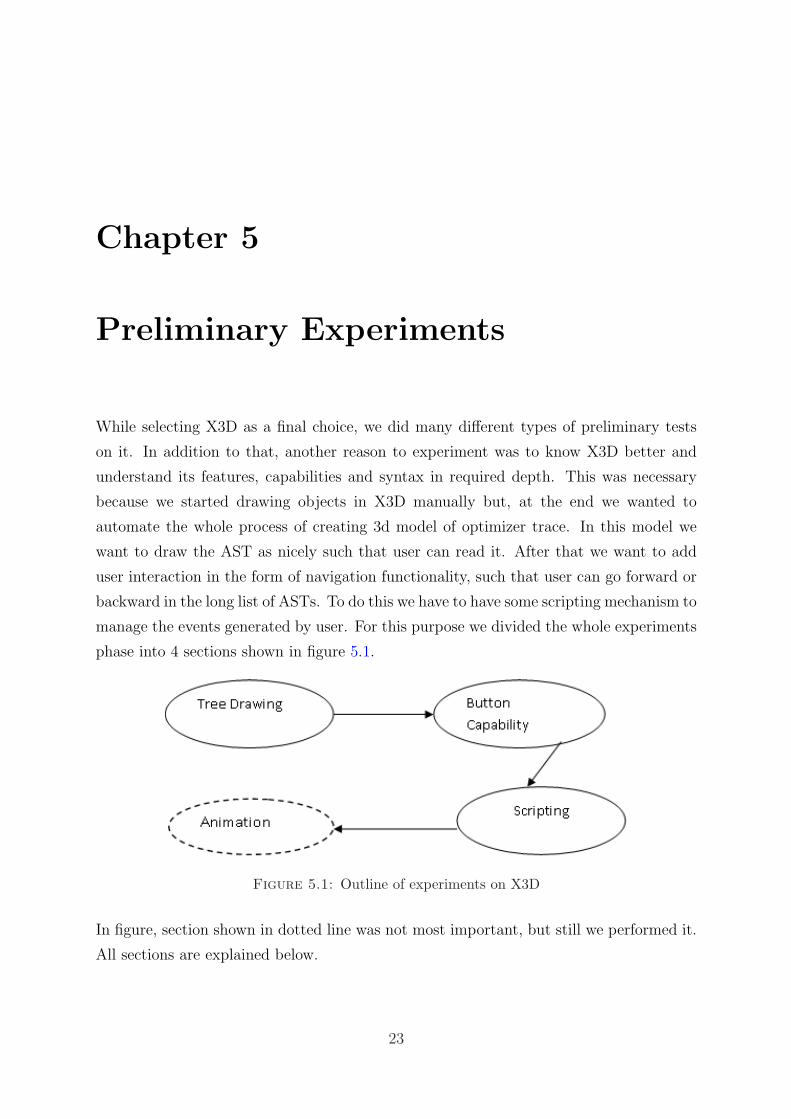
manage the events generated by user. For this purpose we divided the whole experiments
phase into 4 sections shown in figure 5.1.
Figure 5.1: Outline of experiments on X3D
In figure, section shown in dotted line was not most important, but still we performed it.
All sections are explained below.
23
Chapter 5. Preliminary Experiments 24
5.1 Ability To Draw Tree
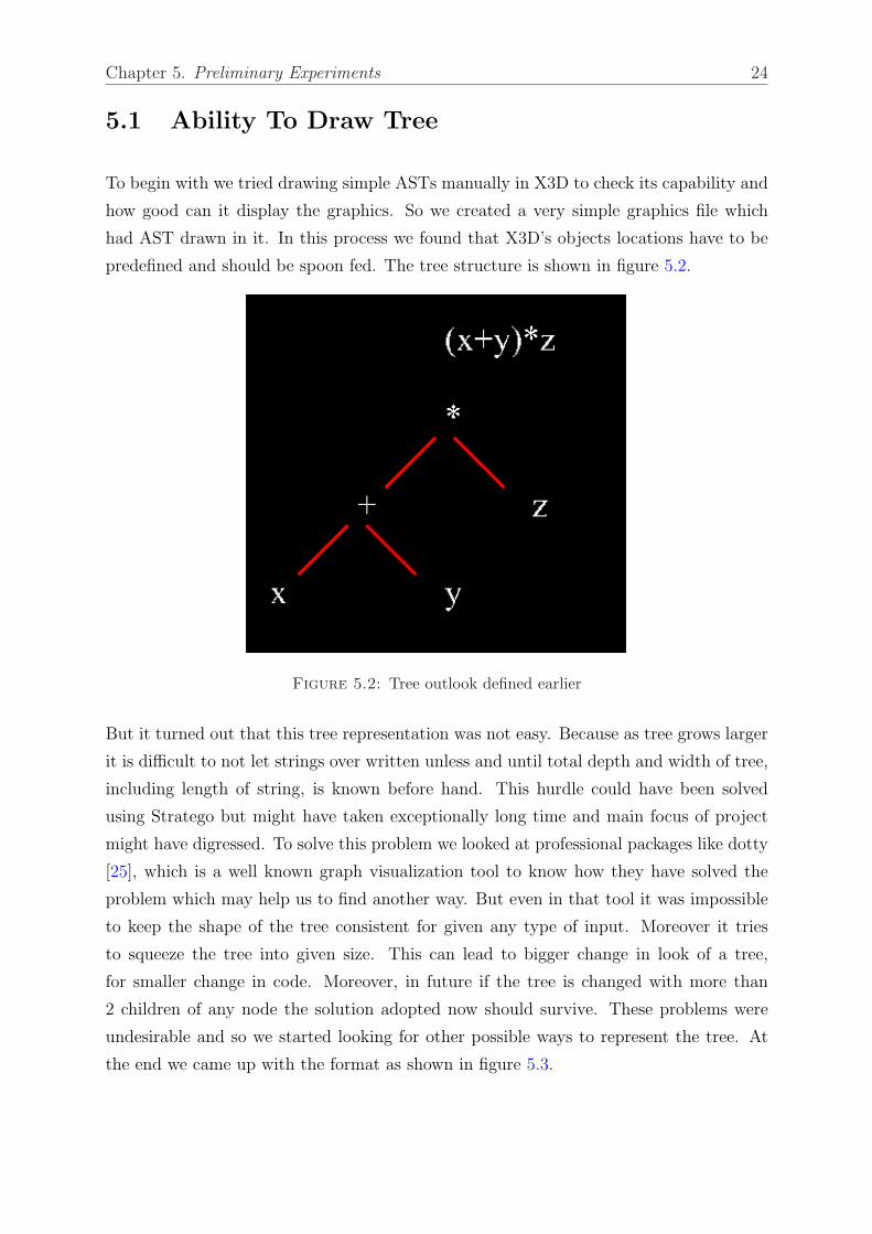
To begin with we tried drawing simple ASTs manually in X3D to check its capability and
how good can it display the graphics. So we created a very simple graphics file which
had AST drawn in it. In this process we found that X3D’s objects locations have to be
predefined and should be spoon fed. The tree structure is shown in figure 5.2.
Figure 5.2: Tree outlook defined earlier
But it turned out that this tree representation was not easy. Because as tree grows larger
it is difficult to not let strings over written unless and until total depth and width of tree,
including length of string, is known before hand. This hurdle could have been solved
using Stratego but might have taken exceptionally long time and main focus of project
might have digressed. To solve this problem we looked at professional packages like dotty
[25], which is a well known graph visualization tool to know how they have solved the
problem which may help us to find another way. But even in that tool it was impossible
to keep the shape of the tree consistent for given any type of input. Moreover it tries
to squeeze the tree into given size. This can lead to bigger change in look of a tree,
for smaller change in code. Moreover, in future if the tree is changed with more than
2 children of any node the solution adopted now should survive. These problems were
undesirable and so we started looking for other possible ways to represent the tree. At
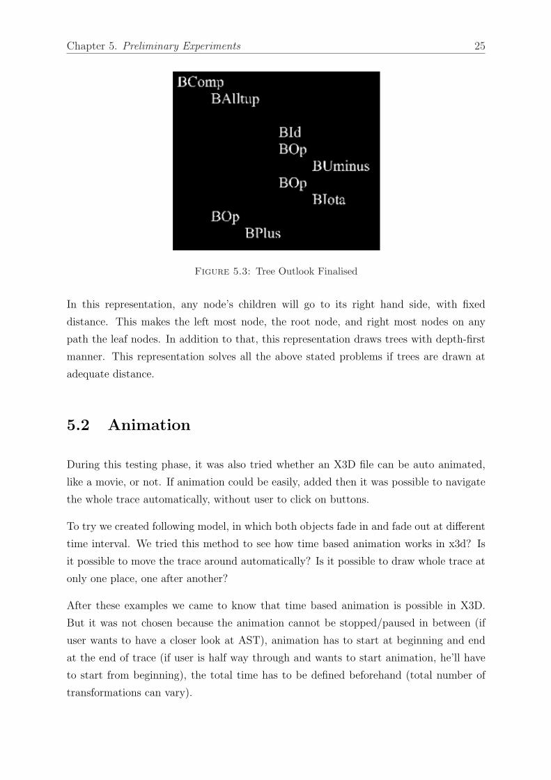
the end we came up with the format as shown in figure 5.3.
Chapter 5. Preliminary Experiments 25
Figure 5.3: Tree Outlook Finalised
In this representation, any node’s children will go to its right hand side, with fixed
distance. This makes the left most node, the root node, and right most nodes on any
path the leaf nodes. In addition to that, this representation draws trees with depth-first
manner. This representation solves all the above stated problems if trees are drawn at
adequate distance.
5.2 Animation
During this testing phase, it was also tried whether an X3D file can be auto animated,
like a movie, or not. If animation could be easily, added then it was possible to navigate
the whole trace automatically, without user to click on buttons.
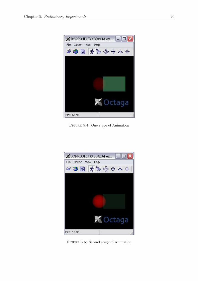
To try we created following model, in which both objects fade in and fade out at different
time interval. We tried this method to see how time based animation works in x3d? Is
it possible to move the trace around automatically? Is it possible to draw whole trace at
only one place, one after another?
After these examples we came to know that time based animation is possible in X3D.
But it was not chosen because the animation cannot be stopped/paused in between (if
user wants to have a closer look at AST), animation has to start at beginning and end
at the end of trace (if user is half way through and wants to start animation, he’ll have
to start from beginning), the total time has to be defined beforehand (total number of
transformations can vary).
Chapter 5. Preliminary Experiments 26
Figure 5.4: One stage of Animation
Figure 5.5: Second stage of Animation
Chapter 5. Preliminary Experiments 27
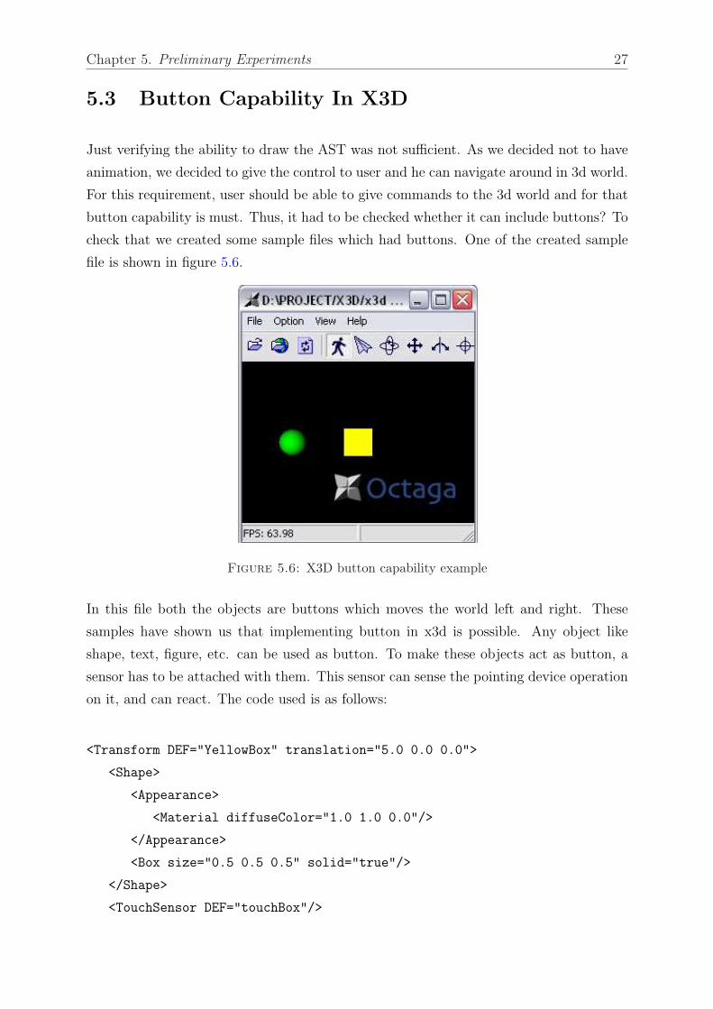
5.3 Button Capability In X3D
Just verifying the ability to draw the AST was not sufficient. As we decided not to have
animation, we decided to give the control to user and he can navigate around in 3d world.
For this requirement, user should be able to give commands to the 3d world and for that
button capability is must. Thus, it had to be checked whether it can include buttons? To
check that we created some sample files which had buttons. One of the created sample
file is shown in figure 5.6.
Figure 5.6: X3D button capability example
In this file both the objects are buttons which moves the world left and right. These
samples have shown us that implementing button in x3d is possible. Any object like
shape, text, figure, etc. can be used as button. To make these objects act as button, a
sensor has to be attached with them. This sensor can sense the pointing device operation
on it, and can react. The code used is as follows:
<Transform DEF="YellowBox" translation="5.0 0.0 0.0">
<Shape>
<Appearance>
<Material diffuseColor="1.0 1.0 0.0"/>
</Appearance>
<Box size="0.5 0.5 0.5" solid="true"/>
</Shape>
<TouchSensor DEF="touchBox"/>
Chapter 5. Preliminary Experiments 28
</Transform>
More about sensors is explained in section 4.8.
5.4 Scripting For User Interactivity
To achieve the required movement and some action, scripts are used widely. It was must
to check whether X3D can support scripting or not? And if it can then how well it can
be used for the project.
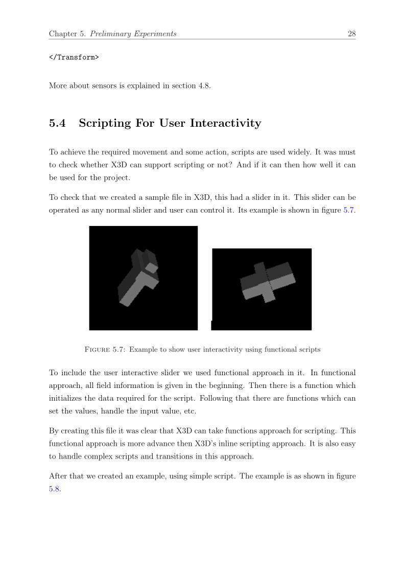
To check that we created a sample file in X3D, this had a slider in it. This slider can be
operated as any normal slider and user can control it. Its example is shown in figure 5.7.
Figure 5.7: Example to show user interactivity using functional scripts
To include the user interactive slider we used functional approach in it. In functional
approach, all field information is given in the beginning. Then there is a function which
initializes the data required for the script. Following that there are functions which can
set the values, handle the input value, etc.
By creating this file it was clear that X3D can take functions approach for scripting. This
functional approach is more advance then X3D’s inline scripting approach. It is also easy
to handle complex scripts and transitions in this approach.
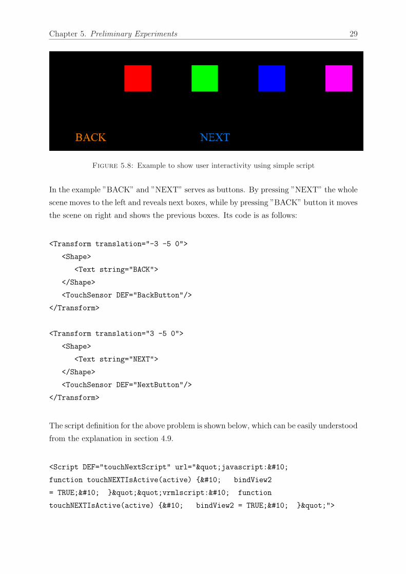
After that we created an example, using simple script. The example is as shown in figure
5.8.
Chapter 5. Preliminary Experiments 29
Figure 5.8: Example to show user interactivity using simple script
In the example ”BACK” and ”NEXT” serves as buttons. By pressing ”NEXT” the whole
scene moves to the left and reveals next boxes, while by pressing ”BACK” button it moves
the scene on right and shows the previous boxes. Its code is as follows:
<Transform translation="-3 -5 0">
<Shape>
<Text string="BACK">
</Shape>
<TouchSensor DEF="BackButton"/>
</Transform>
<Transform translation="3 -5 0">
<Shape>
<Text string="NEXT">
</Shape>
<TouchSensor DEF="NextButton"/>
</Transform>
The script definition for the above problem is shown below, which can be easily understood
from the explanation in section 4.9.
<Script DEF="touchNextScript" url=""javascript:
function touchNEXTIsActive(active) { bindView2
= TRUE; }""vrmlscript: function
touchNEXTIsActive(active) { bindView2 = TRUE; }"">

Chapter 5. Preliminary Experiments 30
<field accessType="inputOnly" name="touchNEXTIsActive" type="SFBool"/>
<field accessType="outputOnly" name="bindView2" type="SFBool"/>
</Script>
Later after trying few other examples, it was revealed that, for this project, embedding
functional approach was more complicated than using simple scripting. Later, we decided
to go for the simple scripting.
In our problem every button (sensor node) and thus every script was slightly different
then each other because, they had to produce different output (move camera to different
location) for similar input (user click). Now, in X3D, scripts cannot take user input. So
the input and output of the functions used in scripts cannot be changed. So, different
outputs cannot be generated from single script. Because of that functional approach
loose its reusability. Furthermore, our problem does not require fancy scripts and so if we
would have implemented functional approach; it might have made the code unnecessarily
bigger as well as might have made the automatic generation of code difficult.
In addition to that, to make the automatic code generation as compact as possible, as
explained earlier we have made every tree and its navigation information local to each
particular AST. Because of this we had to create all the viewpoints earlier so that each
local script can access the global viewpoint and can make the camera move. Because of
these reasons we decided not to use the functional approach but to use the simple scripts.
And this is the same reason why we have 6 scripts attached with every AST.
Different examples have shown that user interactivity is again not easy in X3D but was
possible. It can be achieved in various ways. Just to name a few,
1. By making a text, shape, image or any object a button and then adding script to it
2. By moving the camera and keeping the world as it is
3. By moving the object and keeping remaining world at its place
We have taken combination of approach 1 and 2. However, X3D does not have fancy but-
tons like Adobe Flash, but its current setup serves the required purpose for the project.
Chapter 6
3D Model Generation
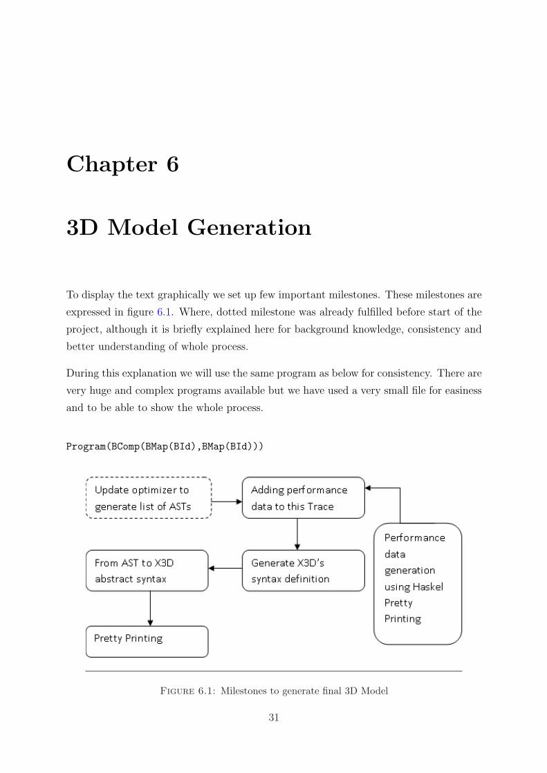
To display the text graphically we set up few important milestones. These milestones are
expressed in figure 6.1. Where, dotted milestone was already fulfilled before start of the
project, although it is briefly explained here for background knowledge, consistency and
better understanding of whole process.
During this explanation we will use the same program as below for consistency. There are
very huge and complex programs available but we have used a very small file for easiness
and to be able to show the whole process.
Program(BComp(BMap(BId),BMap(BId)))
Figure 6.1: Milestones to generate final 3D Model
31
Chapter 6. 3D Model Generation 32
6.1 Generate List Of ASTs
Existing optimizer was able to produce a text dump. This text dump was directly printed
on the go while optimization was in process. Furthermore, it did not include all the
required data. This was of no use for the current project. For further processing the
trace data was needed and thus it has to be stored in systematic way so that it can be
fetched later on. To do that the optimizer was changed to store the trace as it goes on
applying the rules. After doing that, the optimizer was able to create a text dump/trace
which included all the intermediate transformations along with their tree representation.
It was very important to include all the transformations in the trace; otherwise the paths
and the tree, that user looks at, will be out of sync.
At the end of all above operations, a full trace was generated, which included all ASTs
and this trace will look like below.
Program(BTrace([BComp(BMap(BId),BMap(BId)),BComp(BId,BMap(BId)),
BComp(BId,BId),BId]))
Now, this is the kind of trace that we want and have, to work upon and create a 3d model.
During this work, the working of optimizer was understood in detail. It was also learnt
that the optimizer is very flexible and it is very easy to modify it. Also it was found that
application of proper rule at proper time affects the performance a lot.
6.2 Adding Performance Data
After creating a trace, first the performance figures had to be appended to the trace.
This performance figures are currently fetched automatically, and manually appended to
the end of the trace file. Note that this process can also be automated with little effort,
but due to time constraint it was not implemented. We first use the existing bmf hask.pp
file to generate the hask file of any program. For the problem in question, the hask file
will look as follows:
B_trace [ B_comp ( B_map ( B_id ) ) ( B_map ( B_id ) ) ,
B_comp ( B_id ) ( B_map ( B_id ) ) ,
B_comp ( B_id ) ( B_id ) ,
B_id ]

Chapter 6. 3D Model Generation 33
This hask file is then run against existing data to get the efficiency figures. This each
figure shows number of abstract instructions required to run each transformed code. After
running the test data for the above problem, we got following performance figures, which
are then attached at the end of produced trace.
[204,103,2,1]
This will make the trace look like below:
Foo(Program(BTrace([BComp(BMap(BId),BMap(BId)),BComp(BId,BMap(BId)),
BComp(BId,BId),BId])),[204,103,2,1])
The Foo is added in the front manually to put the two lists (list of AST and list of
performance data) in a tuple. This tuple helps to fetch individual lists and then individual
elements from those. This tuple form looks like below:
Foo( LIST , LIST )
After completing this stage, we have a list of AST and list of performance data. Now
it’s time to know how our X3D file look likes, so that, accordingly it can be generated
automatically.
6.3 Generating X3D’s Syntax Definition
As X3D file has to be generated automatically, its full syntax must be known. Moreover
the functionality should be implemented which can generate this syntax. We have divided
this process into following 2 sub processes:
6.3.1 Knowing X3D Syntax
Same X3D files can be created in many ways as it follows the parent-child relationship
format of XML. To create the X3D file effectively from optimizer directly, X3D file’s
required syntax has to be fully explored and should be easy to create from optimizer. To
achieve this goal one X3D file was created which had all required functionality including
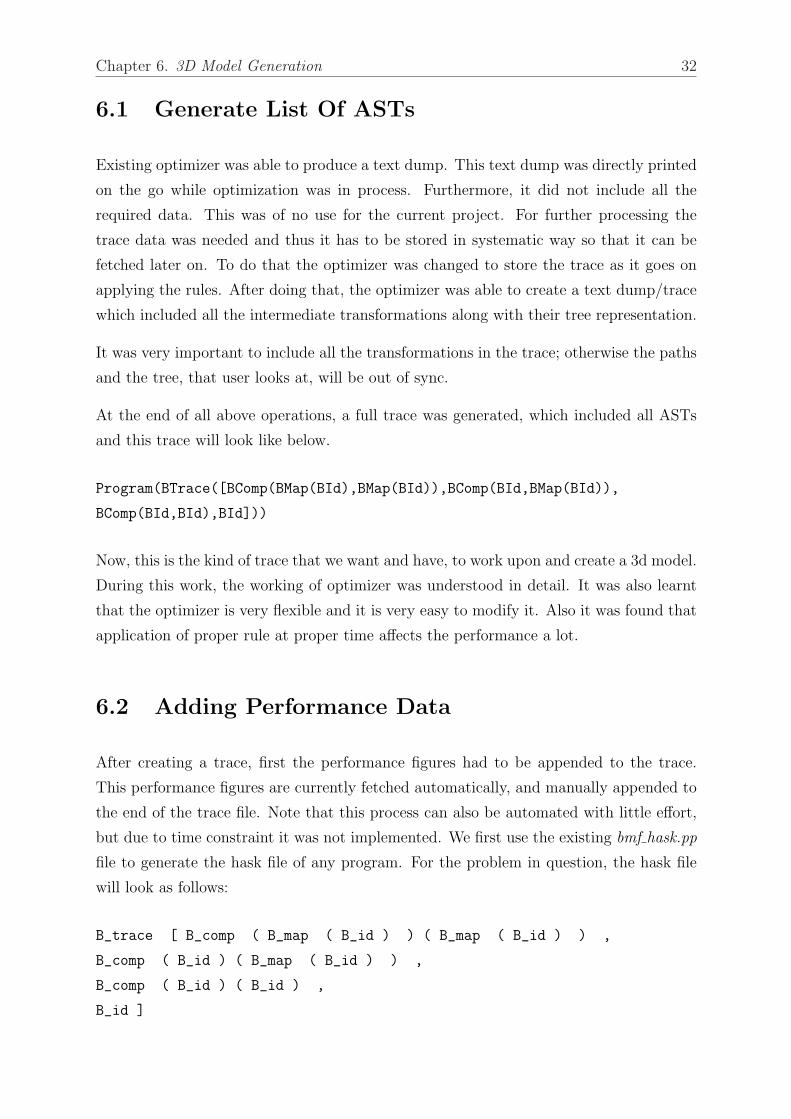
Chapter 6. 3D Model Generation 34
Figure 6.2: First stage file to know x3d syntax, which has to be automatically pro-duced
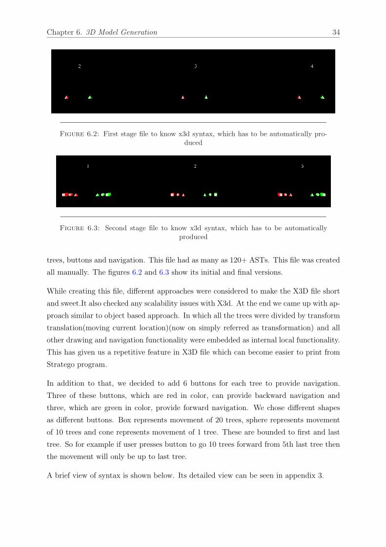
Figure 6.3: Second stage file to know x3d syntax, which has to be automaticallyproduced
trees, buttons and navigation. This file had as many as 120+ ASTs. This file was created
all manually. The figures 6.2 and 6.3 show its initial and final versions.
While creating this file, different approaches were considered to make the X3D file short
and sweet.It also checked any scalability issues with X3d. At the end we came up with ap-
proach similar to object based approach. In which all the trees were divided by transform
translation(moving current location)(now on simply referred as transformation) and all
other drawing and navigation functionality were embedded as internal local functionality.
This has given us a repetitive feature in X3D file which can become easier to print from
Stratego program.
In addition to that, we decided to add 6 buttons for each tree to provide navigation.
Three of these buttons, which are red in color, can provide backward navigation and
three, which are green in color, provide forward navigation. We chose different shapes
as different buttons. Box represents movement of 20 trees, sphere represents movement
of 10 trees and cone represents movement of 1 tree. These are bounded to first and last
tree. So for example if user presses button to go 10 trees forward from 5th last tree then
the movement will only be up to last tree.
A brief view of syntax is shown below. Its detailed view can be seen in appendix 3.
Chapter 6. 3D Model Generation 35
<Viewpoint DEF="View2" description="view object 2" position="20 0 20"/>
<Transform translation="360 0 0">
<Group>
<Shape>
<!-- Draw Tree Here -->
</Shape>
<Transform translation="-2 -5 0">
<!-- Shape with Touch Sensor (Button) -->
</Transform>
... ... ...
<Script -- SCRIPT DEFINITION for button 1 GOES HERE -- >
<!-- Field information goes here -->
</Script>
<ROUTE -- ROUTE INFORMATION for button 1 GOES HERE -- />
<ROUTE -- ROUTE INFORMATION for button 1 GOES HERE -- />
... ... ...
</Group>
</Transform>
In the above shown syntax, all the viewpoints are defined earlier as shown in figure,
giving then unique identifier using DEF. This is required because all scripts are local
to individual transformations and so to move the camera around they should know the
required viewpoints.
After that there is a major transformation which points to the place where tree has to be
drawn. In this transformation everything necessary for one tree is wrapped in a group to
make those thing local and with respect to the transformation. Inside this transformation,
whole tree is drawn, all buttons are added, scripts are added and performance data is
added. Which method we use to draw a tree is irrelevant question here, because tree is
drawn as a child of group, which makes the presentation irrelevant and it just displays.
This is very important feature because if in future we just want to change the tree
representation then we do not have to change whole syntax or whole code. Just the bit
where it draws the tree should be changed.
Inside this group, another transformation is done to draw 6 shapes. We have used cone,
sphere, box and text in whole x3d representation. These shapes are transformed to
different locations to put the shape at that particular location. These transformations
Chapter 6. 3D Model Generation 36
are local. So for common functionality (like navigation buttons) the location remains the
same and makes it easy to automate. Its example can be seen below:
<Transform translation="-2 2 0">
<Shape>
<Appearance>
<Material emissiveColor="1 0 0"/>
</Appearance>
<Cone bottomRadius="0.25" height="0.5"/>
</Shape>
</Transform>
<Transform translation=" 5 -3 0 ">
<Shape>
<Text string="BId" />
</Shape>
</Transform>
A touch sensor is attached to these shapes to make it a button. Its example code is shown
below. In our final code we have used 6 different buttons, where 3 buttons to navigate
forward and 3 to navigate backward. We have allowed user to navigate 1 transformation
(using shape cone), 10 transformations (using shape sphere) or 20 transformations (using
shape box) forward (green color buttons) or backward (red color buttons) at a time.
This can be easily changed to any required amount. One of its examples (red cone -1
transformation backward) can be seen below:
<Transform translation="-2 -5 0">
<Shape>
<Appearance>
<Material emissiveColor="1 0 0"/>
</Appearance>
<Cone bottomRadius="0.25" height="0.5"/>
</Shape>
<TouchSensor DEF="Back_1" description="Back button for object 1"/>
</Transform>

Chapter 6. 3D Model Generation 37
After adding the button a script should be added to handle the user events. The example
code is shown below, which shows which format to use. This code is designed such that
it can be reused in whole 3D model with minimal changes.
<Script DEF="Script_Back_Single_1" url=""javascript:
function Back_Single_1IsActive(active)
{ bindView1= TRUE; }""vrmlscript:
function Back_Single_1IsActive(active)
{ bindView1 = TRUE; }"">
<field accessType="inputOnly" name="Back_Single_1IsActive"
type="SFBool"/>
<field accessType="outputOnly" name="bindView1" type="SFBool"/>
</Script>
<ROUTE fromField="isActive" fromNode="Back_Single_1"
toField="Back_Single_1IsActive" toNode="Script_Back_Single_1"/>
<ROUTE fromField="bindView1" fromNode="Script_Back_Single_1"
toField="set_bind" toNode="View1"/>
6.3.2 Generating X3D Syntax
To generate this syntax all the parent child relation has to be finalized. It was also
necessary to know the data each node has to have. For example, Transform node should
know to which location it has to transform, shape node should know its size and color
etc. All these details were gathered from the giant file created manually.
The following syntax definition and signature files were created in smaller increments by
adding required functionality at a time. For instance, initially only tree was drawn, so
only syntax required for that was defined, later on Buttons were added and after that
navigational scripts were added.
Now, to create the syntax definition X3D’s literals had to be defined first. While creating
X3D abstract syntax, these literals allow transfer of data. They are defined in a similar
way of any other literals. For example positive float is defined by any number of digits,
followed by ”.”, followed by one or more number of digits, combination of positive float
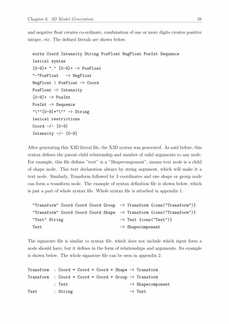
Chapter 6. 3D Model Generation 38
and negative float creates co-ordinate, combination of one or more digits creates positive
integer, etc. The defined literals are shown below.
sorts Coord Intensity String PosFloat NegFloat PosInt Sequence
lexical syntax
[0-9]* "." [0-9]+ -> PosFloat
"-"PosFloat -> NegFloat
NegFloat | PosFloat -> Coord
PosFloat -> Intensity
[0-9]+ -> PosInt
PosInt -> Sequence
"\""[0-9]*"\"" -> String
lexical restrictions
Coord -/- [0-9]
Intensity -/- [0-9]
After generating this X3D literal file, the X3D syntax was generated. As said before, this
syntax defines the parent child relationship and number of valid arguments to any node.
For example, this file defines ”text” is a ”Shapecomponent”, means text node is a child
of shape node. This text declaration always by string argument, which will make it a
text node. Similarly, Transform followed by 3 coordinates and one shape or group node
can form a transform node. The example of syntax definition file is shown below, which
is just a part of whole syntax file. Whole syntax file is attached in appendix 1.
"Transform" Coord Coord Coord Group -> Transform {cons("Transform")}
"Transform" Coord Coord Coord Shape -> Transform {cons("Transform")}
"Text" String -> Text {cons("Text")}
Text -> Shapecomponent
The signature file is similar to syntax file, which does not include which input form a
node should have, but it defines in the form of relationships and arguments. Its example
is shown below. The whole signature file can be seen in appendix 2.
Transform : Coord * Coord * Coord * Shape -> Transform
Transform : Coord * Coord * Coord * Group -> Transform
: Text -> Shapecomponent
Text : String -> Text
Chapter 6. 3D Model Generation 39
6.4 From AST To X3D Abstract Syntax
After generating X3D syntax definitions, now the road was clear to convert AST into
X3D abstract syntax. To do that a program is created which takes trace of ASTs from
optimizer, X3D syntax definition and creates an X3D file with abstract syntax. X3D
abstract syntax file includes all the necessary viewpoints and trees. The remaining items
are added in the next phase.
6.4.1 Generating Viewpoints
One of the requirements of X3D file was that all the viewpoints1 have to be declared in
the beginning of the file. This was because, when individual transformations want to
navigate around, they should have definition for required view point. This definition is
similar to global variables in any functional language.
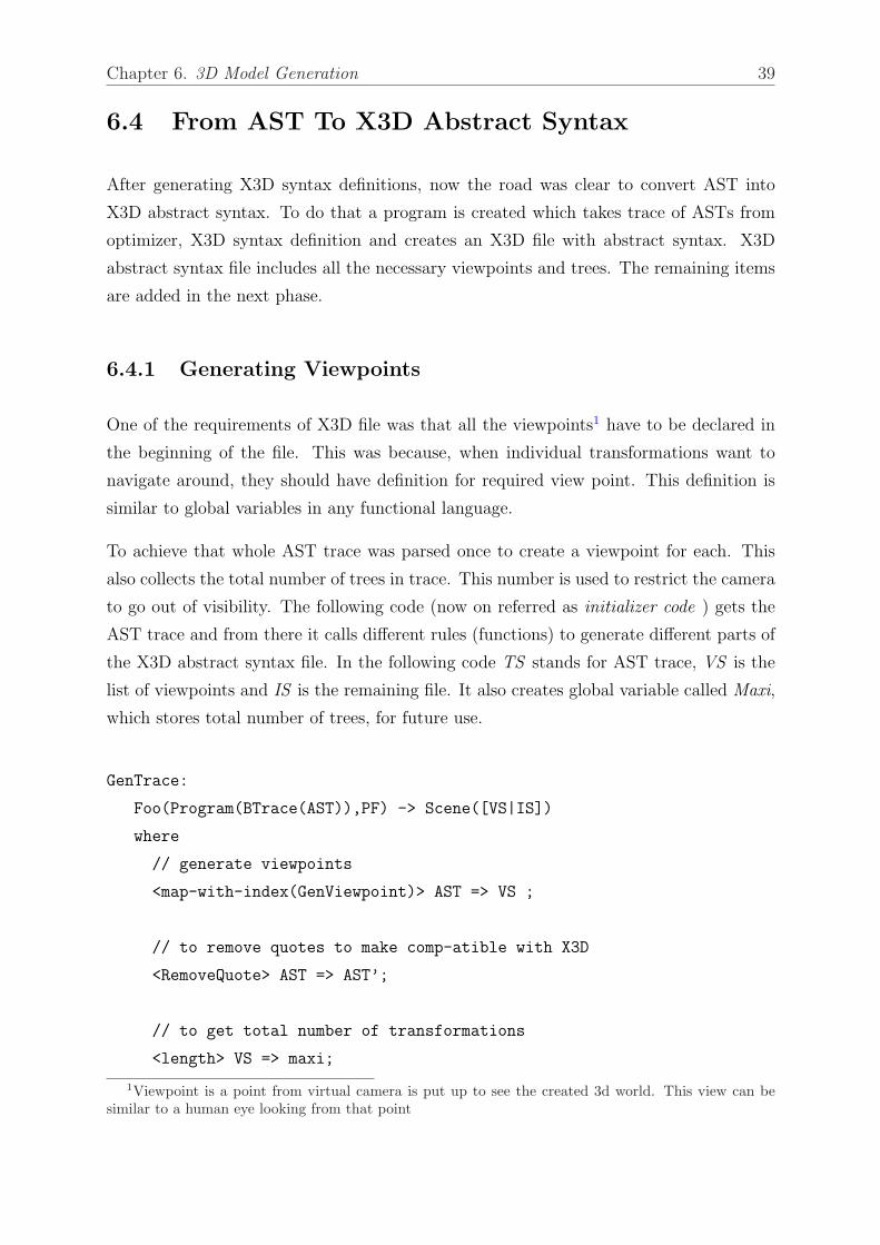
To achieve that whole AST trace was parsed once to create a viewpoint for each. This
also collects the total number of trees in trace. This number is used to restrict the camera
to go out of visibility. The following code (now on referred as initializer code ) gets the
AST trace and from there it calls different rules (functions) to generate different parts of
the X3D abstract syntax file. In the following code TS stands for AST trace, VS is the
list of viewpoints and IS is the remaining file. It also creates global variable called Maxi,
which stores total number of trees, for future use.
GenTrace:
Foo(Program(BTrace(AST)),PF) -> Scene([VS|IS])
where
// generate viewpoints
<map-with-index(GenViewpoint)> AST => VS ;
// to remove quotes to make comp-atible with X3D
<RemoveQuote> AST => AST’;
// to get total number of transformations
<length> VS => maxi;
1Viewpoint is a point from virtual camera is put up to see the created 3d world. This view can besimilar to a human eye looking from that point
Chapter 6. 3D Model Generation 40
// prints total number of trees in the trace
debug(!"Total number of trees are -> ");
rules( Maxi:= maxi );
rules( Performance:=PF);
// generates trees
<map-with-index(GenOneTree)> AST’ => IS
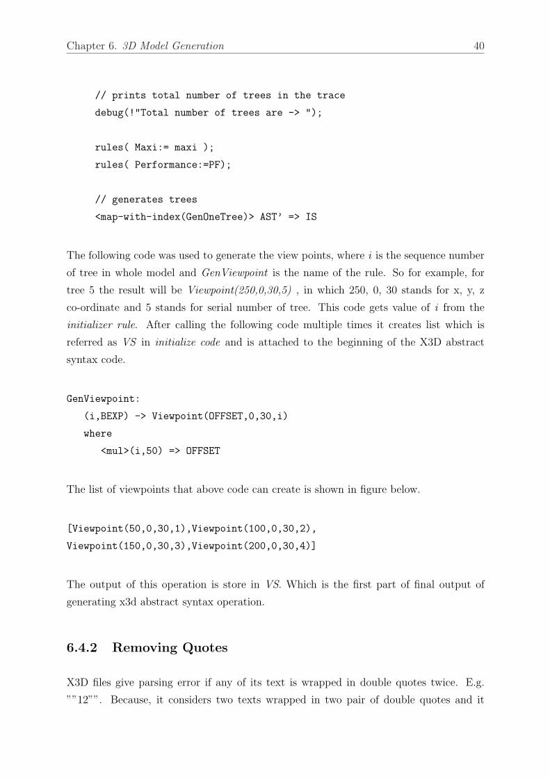
The following code was used to generate the view points, where i is the sequence number
of tree in whole model and GenViewpoint is the name of the rule. So for example, for
tree 5 the result will be Viewpoint(250,0,30,5) , in which 250, 0, 30 stands for x, y, z
co-ordinate and 5 stands for serial number of tree. This code gets value of i from the
initializer rule. After calling the following code multiple times it creates list which is
referred as VS in initialize code and is attached to the beginning of the X3D abstract
syntax code.
GenViewpoint:
(i,BEXP) -> Viewpoint(OFFSET,0,30,i)
where
<mul>(i,50) => OFFSET
The list of viewpoints that above code can create is shown in figure below.
[Viewpoint(50,0,30,1),Viewpoint(100,0,30,2),
Viewpoint(150,0,30,3),Viewpoint(200,0,30,4)]
The output of this operation is store in VS. Which is the first part of final output of
generating x3d abstract syntax operation.
6.4.2 Removing Quotes
X3D files give parsing error if any of its text is wrapped in double quotes twice. E.g.
””12””. Because, it considers two texts wrapped in two pair of double quotes and it
Chapter 6. 3D Model Generation 41
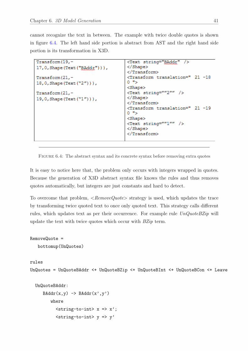
cannot recognize the text in between. The example with twice double quotes is shown
in figure 6.4. The left hand side portion is abstract from AST and the right hand side
portion is its transformation in X3D.
Figure 6.4: The abstract syntax and its concrete syntax before removing extra quotes
It is easy to notice here that, the problem only occurs with integers wrapped in quotes.
Because the generation of X3D abstract syntax file knows the rules and thus removes
quotes automatically, but integers are just constants and hard to detect.
To overcome that problem, <RemoveQuote> strategy is used, which updates the trace
by transforming twice quoted text to once only quoted text. This strategy calls different
rules, which updates text as per their occurrence. For example rule UnQuoteBZip will
update the text with twice quotes which occur with BZip term.
RemoveQuote =
bottomup(UnQuotes)
rules
UnQuotes = UnQuoteBAddr <+ UnQuoteBZip <+ UnQuoteBInt <+ UnQuoteBCon <+ Leave
UnQuoteBAddr:
BAddr(x,y) -> BAddr(x’,y’)
where
<string-to-int> x => x’;
<string-to-int> y => y’
Chapter 6. 3D Model Generation 42
UnQuoteBZip:
BZip(x) -> BZip(x’)
where
<string-to-int> x => x’
UnQuoteBInt:
BInt(x) -> BInt(x’)
where
<string-to-int> x => x’
UnQuoteBCon:
BCon(x) -> BCon(x’)
where
<string-to-int> x => x’
Leave:
x -> x
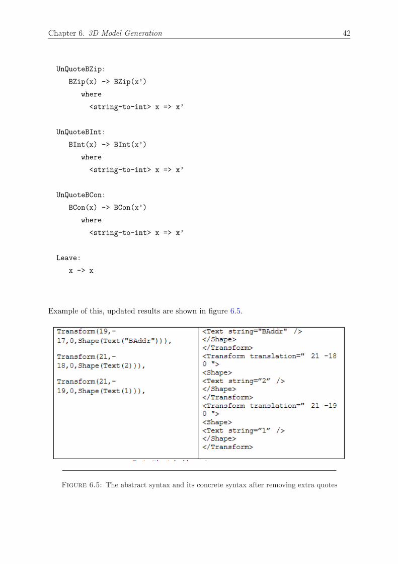
Example of this, updated results are shown in figure 6.5.
Figure 6.5: The abstract syntax and its concrete syntax after removing extra quotes
Chapter 6. 3D Model Generation 43
6.4.3 Getting Indentation For Tree
To get the location where to transform, we have pre parsing stage where indenting is
calculated. Its code is as follows. Where, recursive call to MapIndent increases X co-
ordinate for child node. On the other hand, the Y co-ordinate indenting is decided, when
the text is being printed.
MapIndent (|n) =
?c#(ts);
<map (MapIndent (|<add>(2,n)))> ts => res;
<concat> res => res1;
<conc> ( [(c,n)] ,res1) => res2
The output of that is indentation is appended to every node text. The example is shown
below.
[("BComp",1),("BMap",3),("BId",5),("BMap",3),("BId",5)]
The terms 1, 3, 5 are indentation on x axis. For indentation on Y axis we just have to
print each text below the previous one so we have just decreased location on Y axis by 1
with every node.
At the end of this stage skeleton of the X3d abstract syntax file was ready and it was the
time to actually put information (AST in our case) in the skeleton.
6.4.4 Printing Text
The initizlizer code will then start making the remaining part of the X3D abstract syntax
file, which includes all trees. As only trees will be drawn from this stage, it will have to
print only text and align it to represent in tree form. The following code will simply draw
the tree at given location. GenNode is the name of the rule. The Transform part in the
code will transform at the certain location and Shape(Text()) will print the text.
GenNode:
(y,(name,X)) -> Transform(X,Y,0,Shape(Text(name)))
where
<mul>(-1,y) => Y
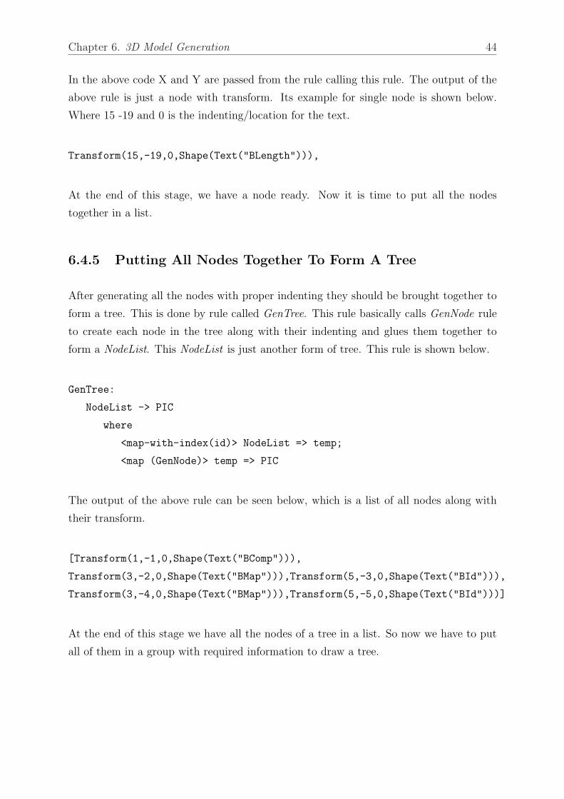
Chapter 6. 3D Model Generation 44
In the above code X and Y are passed from the rule calling this rule. The output of the
above rule is just a node with transform. Its example for single node is shown below.
Where 15 -19 and 0 is the indenting/location for the text.
Transform(15,-19,0,Shape(Text("BLength"))),
At the end of this stage, we have a node ready. Now it is time to put all the nodes
together in a list.
6.4.5 Putting All Nodes Together To Form A Tree
After generating all the nodes with proper indenting they should be brought together to
form a tree. This is done by rule called GenTree. This rule basically calls GenNode rule
to create each node in the tree along with their indenting and glues them together to
form a NodeList. This NodeList is just another form of tree. This rule is shown below.
GenTree:
NodeList -> PIC
where
<map-with-index(id)> NodeList => temp;
<map (GenNode)> temp => PIC
The output of the above rule can be seen below, which is a list of all nodes along with
their transform.
[Transform(1,-1,0,Shape(Text("BComp"))),
Transform(3,-2,0,Shape(Text("BMap"))),Transform(5,-3,0,Shape(Text("BId"))),
Transform(3,-4,0,Shape(Text("BMap"))),Transform(5,-5,0,Shape(Text("BId")))]
At the end of this stage we have all the nodes of a tree in a list. So now we have to put
all of them in a group with required information to draw a tree.
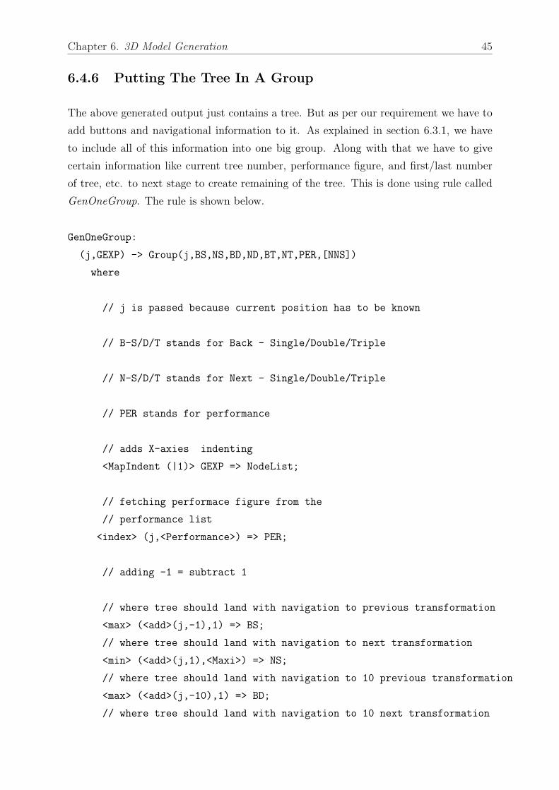
Chapter 6. 3D Model Generation 45
6.4.6 Putting The Tree In A Group
The above generated output just contains a tree. But as per our requirement we have to
add buttons and navigational information to it. As explained in section 6.3.1, we have
to include all of this information into one big group. Along with that we have to give
certain information like current tree number, performance figure, and first/last number
of tree, etc. to next stage to create remaining of the tree. This is done using rule called
GenOneGroup. The rule is shown below.
GenOneGroup:
(j,GEXP) -> Group(j,BS,NS,BD,ND,BT,NT,PER,[NNS])
where
// j is passed because current position has to be known
// B-S/D/T stands for Back - Single/Double/Triple
// N-S/D/T stands for Next - Single/Double/Triple
// PER stands for performance
// adds X-axies indenting
<MapIndent (|1)> GEXP => NodeList;
// fetching performace figure from the
// performance list
<index> (j,<Performance>) => PER;
// adding -1 = subtract 1
// where tree should land with navigation to previous transformation
<max> (<add>(j,-1),1) => BS;
// where tree should land with navigation to next transformation
<min> (<add>(j,1),<Maxi>) => NS;
// where tree should land with navigation to 10 previous transformation
<max> (<add>(j,-10),1) => BD;
// where tree should land with navigation to 10 next transformation
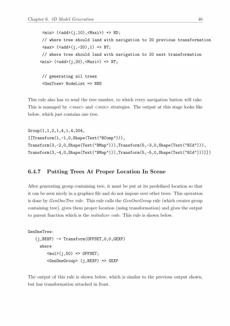
Chapter 6. 3D Model Generation 46
<min> (<add>(j,10),<Maxi>) => ND;
// where tree should land with navigation to 20 previous transformation
<max> (<add>(j,-20),1) => BT;
// where tree should land with navigation to 20 next transformation
<min> (<add>(j,20),<Maxi>) => NT;
// generating all trees
<GenTree> NodeList => NNS
This rule also has to send the tree number, to which every navigation button will take.
This is managed by <max> and <min> strategies. The output at this stage looks like
below, which just contains one tree.
Group(1,1,2,1,4,1,4,204,
[[Transform(1,-1,0,Shape(Text("BComp"))),
Transform(3,-2,0,Shape(Text("BMap"))),Transform(5,-3,0,Shape(Text("BId"))),
Transform(3,-4,0,Shape(Text("BMap"))),Transform(5,-5,0,Shape(Text("BId")))]])
6.4.7 Putting Trees At Proper Location In Scene
After generating group containing tree, it must be put at its predefined location so that
it can be seen nicely in a graphics file and do not impose over other trees. This operation
is done by GenOneTree rule. This rule calls the GenOneGroup rule (which creates group
containing tree), gives them proper location (using transformation) and gives the output
to parent function which is the initializer code. This rule is shown below.
GenOneTree:
(j,BEXP) -> Transform(OFFSET,0,0,GEXP)
where
<mul>(j,50) => OFFSET;
<GenOneGroup> (j,BEXP) => GEXP
The output of this rule is shown below, which is similar to the previous output shown,
but has transformation attached in front.
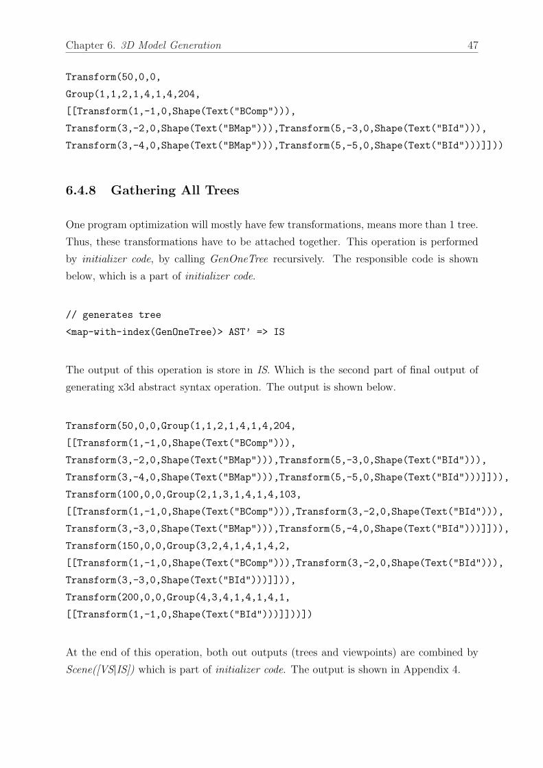
Chapter 6. 3D Model Generation 47
Transform(50,0,0,
Group(1,1,2,1,4,1,4,204,
[[Transform(1,-1,0,Shape(Text("BComp"))),
Transform(3,-2,0,Shape(Text("BMap"))),Transform(5,-3,0,Shape(Text("BId"))),
Transform(3,-4,0,Shape(Text("BMap"))),Transform(5,-5,0,Shape(Text("BId")))]]))
6.4.8 Gathering All Trees
One program optimization will mostly have few transformations, means more than 1 tree.
Thus, these transformations have to be attached together. This operation is performed
by initializer code, by calling GenOneTree recursively. The responsible code is shown
below, which is a part of initializer code.
// generates tree
<map-with-index(GenOneTree)> AST’ => IS
The output of this operation is store in IS. Which is the second part of final output of
generating x3d abstract syntax operation. The output is shown below.
Transform(50,0,0,Group(1,1,2,1,4,1,4,204,
[[Transform(1,-1,0,Shape(Text("BComp"))),
Transform(3,-2,0,Shape(Text("BMap"))),Transform(5,-3,0,Shape(Text("BId"))),
Transform(3,-4,0,Shape(Text("BMap"))),Transform(5,-5,0,Shape(Text("BId")))]])),
Transform(100,0,0,Group(2,1,3,1,4,1,4,103,
[[Transform(1,-1,0,Shape(Text("BComp"))),Transform(3,-2,0,Shape(Text("BId"))),
Transform(3,-3,0,Shape(Text("BMap"))),Transform(5,-4,0,Shape(Text("BId")))]])),
Transform(150,0,0,Group(3,2,4,1,4,1,4,2,
[[Transform(1,-1,0,Shape(Text("BComp"))),Transform(3,-2,0,Shape(Text("BId"))),
Transform(3,-3,0,Shape(Text("BId")))]])),
Transform(200,0,0,Group(4,3,4,1,4,1,4,1,
[[Transform(1,-1,0,Shape(Text("BId")))]]))])
At the end of this operation, both out outputs (trees and viewpoints) are combined by
Scene([VS|IS]) which is part of initializer code. The output is shown in Appendix 4.
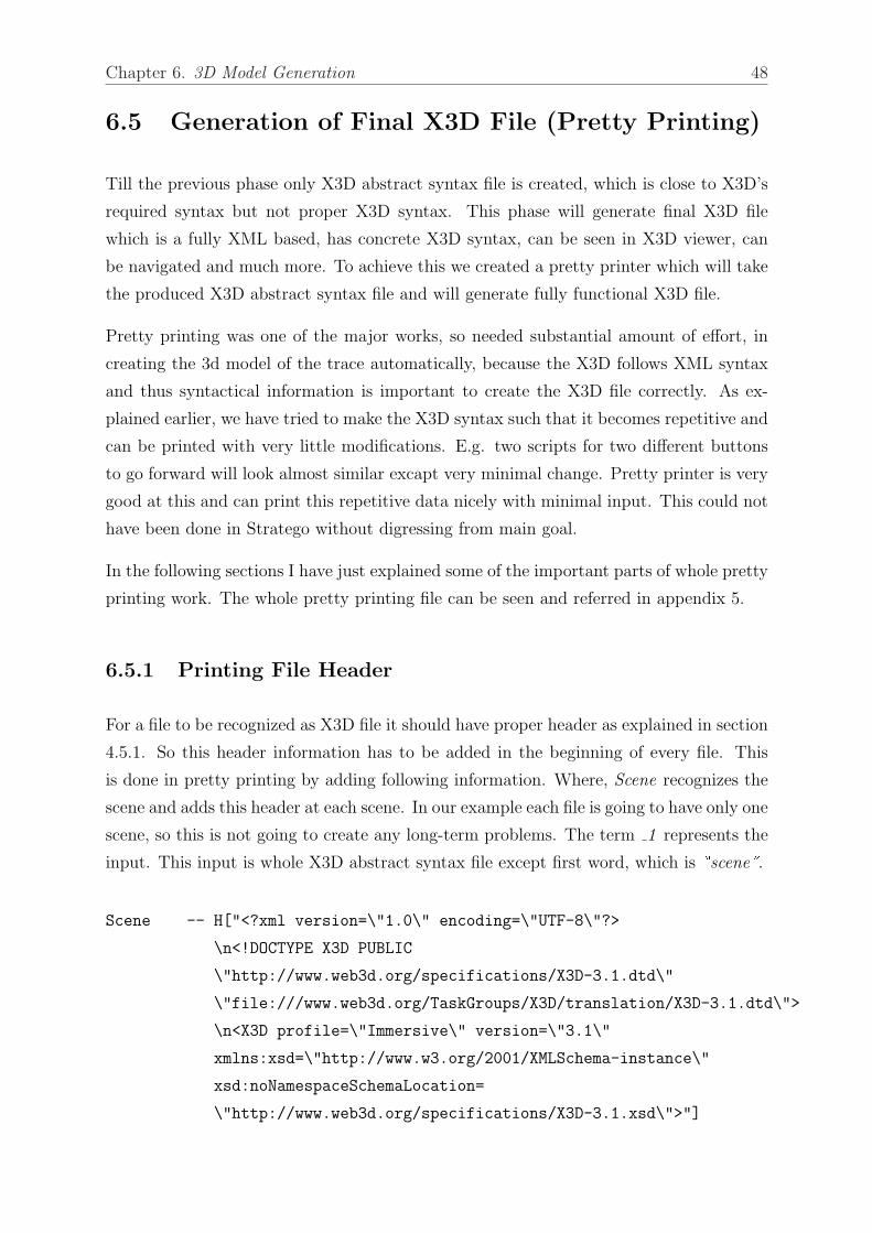
Chapter 6. 3D Model Generation 48
6.5 Generation of Final X3D File (Pretty Printing)
Till the previous phase only X3D abstract syntax file is created, which is close to X3D’s
required syntax but not proper X3D syntax. This phase will generate final X3D file
which is a fully XML based, has concrete X3D syntax, can be seen in X3D viewer, can
be navigated and much more. To achieve this we created a pretty printer which will take
the produced X3D abstract syntax file and will generate fully functional X3D file.
Pretty printing was one of the major works, so needed substantial amount of effort, in
creating the 3d model of the trace automatically, because the X3D follows XML syntax
and thus syntactical information is important to create the X3D file correctly. As ex-
plained earlier, we have tried to make the X3D syntax such that it becomes repetitive and
can be printed with very little modifications. E.g. two scripts for two different buttons
to go forward will look almost similar excapt very minimal change. Pretty printer is very
good at this and can print this repetitive data nicely with minimal input. This could not
have been done in Stratego without digressing from main goal.
In the following sections I have just explained some of the important parts of whole pretty
printing work. The whole pretty printing file can be seen and referred in appendix 5.
6.5.1 Printing File Header
For a file to be recognized as X3D file it should have proper header as explained in section
4.5.1. So this header information has to be added in the beginning of every file. This
is done in pretty printing by adding following information. Where, Scene recognizes the
scene and adds this header at each scene. In our example each file is going to have only one
scene, so this is not going to create any long-term problems. The term 1 represents the
input. This input is whole X3D abstract syntax file except first word, which is �scene�.
Scene -- H["<?xml version=\"1.0\" encoding=\"UTF-8\"?>
\n<!DOCTYPE X3D PUBLIC
\"http://www.web3d.org/specifications/X3D-3.1.dtd\"
\"file:///www.web3d.org/TaskGroups/X3D/translation/X3D-3.1.dtd\">
\n<X3D profile=\"Immersive\" version=\"3.1\"
xmlns:xsd=\"http://www.w3.org/2001/XMLSchema-instance\"
xsd:noNamespaceSchemaLocation=
\"http://www.web3d.org/specifications/X3D-3.1.xsd\">"]
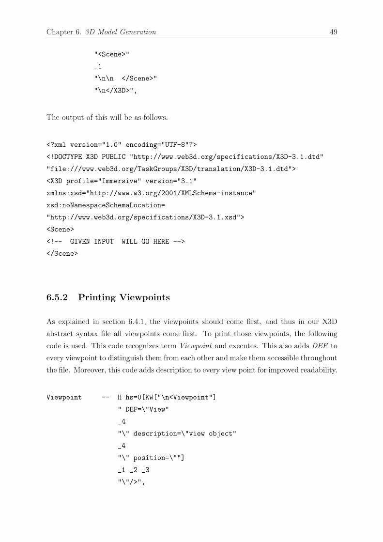
Chapter 6. 3D Model Generation 49
"<Scene>"
_1
"\n\n </Scene>"
"\n</X3D>",
The output of this will be as follows.
<?xml version="1.0" encoding="UTF-8"?>
<!DOCTYPE X3D PUBLIC "http://www.web3d.org/specifications/X3D-3.1.dtd"
"file:///www.web3d.org/TaskGroups/X3D/translation/X3D-3.1.dtd">
<X3D profile="Immersive" version="3.1"
xmlns:xsd="http://www.w3.org/2001/XMLSchema-instance"
xsd:noNamespaceSchemaLocation=
"http://www.web3d.org/specifications/X3D-3.1.xsd">
<Scene>
<!-- GIVEN INPUT WILL GO HERE -->
</Scene>
6.5.2 Printing Viewpoints
As explained in section 6.4.1, the viewpoints should come first, and thus in our X3D
abstract syntax file all viewpoints come first. To print those viewpoints, the following
code is used. This code recognizes term Viewpoint and executes. This also adds DEF to
every viewpoint to distinguish them from each other and make them accessible throughout
the file. Moreover, this code adds description to every view point for improved readability.
Viewpoint -- H hs=0[KW["\n<Viewpoint"]
" DEF=\"View"
_4
"\" description=\"view object"
_4
"\" position=\""]
_1 _2 _3
"\"/>",
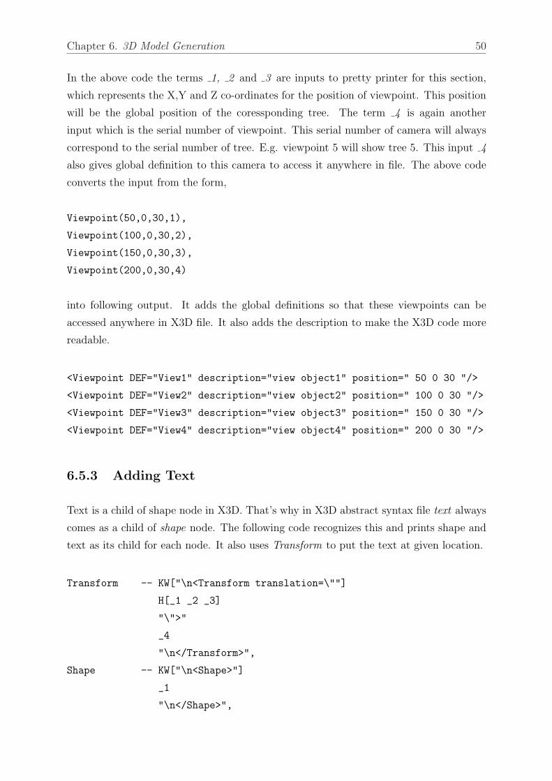
Chapter 6. 3D Model Generation 50
In the above code the terms 1, 2 and 3 are inputs to pretty printer for this section,
which represents the X,Y and Z co-ordinates for the position of viewpoint. This position
will be the global position of the coressponding tree. The term 4 is again another
input which is the serial number of viewpoint. This serial number of camera will always
correspond to the serial number of tree. E.g. viewpoint 5 will show tree 5. This input 4
also gives global definition to this camera to access it anywhere in file. The above code
converts the input from the form,
Viewpoint(50,0,30,1),
Viewpoint(100,0,30,2),
Viewpoint(150,0,30,3),
Viewpoint(200,0,30,4)
into following output. It adds the global definitions so that these viewpoints can be
accessed anywhere in X3D file. It also adds the description to make the X3D code more
readable.
<Viewpoint DEF="View1" description="view object1" position=" 50 0 30 "/>
<Viewpoint DEF="View2" description="view object2" position=" 100 0 30 "/>
<Viewpoint DEF="View3" description="view object3" position=" 150 0 30 "/>
<Viewpoint DEF="View4" description="view object4" position=" 200 0 30 "/>
6.5.3 Adding Text
Text is a child of shape node in X3D. That’s why in X3D abstract syntax file text always
comes as a child of shape node. The following code recognizes this and prints shape and
text as its child for each node. It also uses Transform to put the text at given location.
Transform -- KW["\n<Transform translation=\""]
H[_1 _2 _3]
"\">"
_4
"\n</Transform>",
Shape -- KW["\n<Shape>"]
_1
"\n</Shape>",
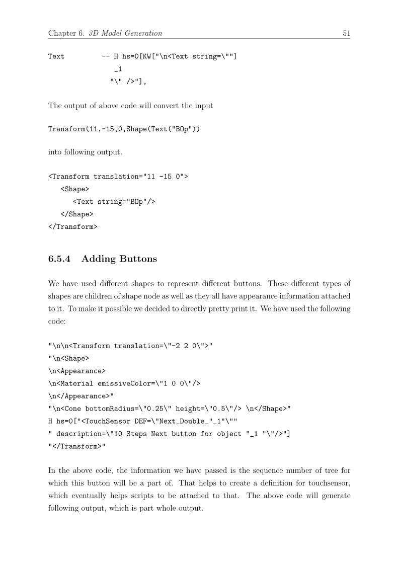
Chapter 6. 3D Model Generation 51
Text -- H hs=0[KW["\n<Text string=\""]
_1
"\" />"],
The output of above code will convert the input
Transform(11,-15,0,Shape(Text("BOp"))
into following output.
<Transform translation="11 -15 0">
<Shape>
<Text string="BOp"/>
</Shape>
</Transform>
6.5.4 Adding Buttons
We have used different shapes to represent different buttons. These different types of
shapes are children of shape node as well as they all have appearance information attached
to it. To make it possible we decided to directly pretty print it. We have used the following
code:
"\n\n<Transform translation=\"-2 2 0\">"
"\n<Shape>
\n<Appearance>
\n<Material emissiveColor=\"1 0 0\"/>
\n</Appearance>"
"\n<Cone bottomRadius=\"0.25\" height=\"0.5\"/> \n</Shape>"
H hs=0["<TouchSensor DEF=\"Next_Double_"_1"\""
" description=\"10 Steps Next button for object "_1 "\"/>"]
"</Transform>"
In the above code, the information we have passed is the sequence number of tree for
which this button will be a part of. That helps to create a definition for touchsensor,
which eventually helps scripts to be attached to that. The above code will generate
following output, which is part whole output.

Chapter 6. 3D Model Generation 52
<Transform translation="-2 2 0">
<Shape>
<Appearance>
<Material emissiveColor="1 0 0"/>
</Appearance>
<Sphere radius="0.25" solid="true"/>
</Shape>
<TouchSensor DEF="Next_Double_1"
description="10 Steps Next button for object 1"/>
</Transform>
6.5.5 Adding Script And Route Information
Similar to buttons, script and route information is also pretty printed. We used the
following code to generate scripts and route.
H hs=0[
"\n<Script DEF=\"Script_Back_Single_" _1 "\""
" url=\""javascript: "
" function Back_Single_" _1 "IsActive(active)"
" { bindView" _1 "= TRUE; }""vrmlscript: "
" function Back_Single_" _1 "IsActive(active)"
" { bindView" _1 " = TRUE; }"\"> "
"\n<field accessType=\"inputOnly\" name=\"Back_Single_"_1"IsActive\"
type=\"SFBool\"/>"
"\n<field accessType=\"outputOnly\" name=\"bindView"_1"\" type=\"SFBool\"/>"
"\n</Script>"
"\n<ROUTE fromField=\"isActive\" fromNode=\"Back_Single_"_1"\""
"\n toField=\"Back_Single_"_1"IsActive\""
" toNode=\"Script_Back_Single_"_1"\"/>"
"\n<ROUTE fromField=\"bindView"_1"\" fromNode=\"Script_Back_Single_"_1"\" "
"\n toField=\"set_bind\""
" toNode=\"View"_2"\"/>"
In this code, it was necessary to give information about, where to move the camera on
user input. This will differ slightly for every button and thus for every script. This script

Chapter 6. 3D Model Generation 53
also have to refer to global viewpoints. So which viewpoint to refer is also given as a
parameter. The output will be as below:
<Script DEF="Script_Back_Single_1" url=""javascript: function Back_Single_1IsActive(active) { bindView1= TRUE; }""vrmlscript: function Back_Single_1IsActive(active) { bindView1 = TRUE; }"">
<field accessType="inputOnly" name="Back_Single_1IsActive" type="SFBool"/>
<field accessType="outputOnly" name="bindView1" type="SFBool"/>
</Script>
<ROUTE fromField="isActive" fromNode="Back_Single_1"
toField="Back_Single_1IsActive" toNode="Script_Back_Single_1"/>
<ROUTE fromField="bindView1" fromNode="Script_Back_Single_1"
toField="set_bind" toNode="View1"/>

Chapter 7
Results
As stated earlier the whole trace generation was done in separate stages after generating
AST trace. The output in X3D at different stages is shown below. The images are little
bit distorted because they had to be managed to fit in appropriate size. The example
taken is in the continuity of previous chapter,which is very basic one, so that whole tree
can be shown in image of appropriate size.
54
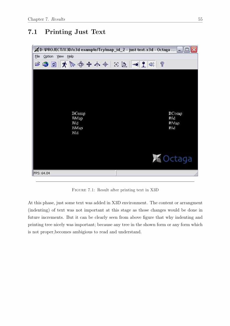
Chapter 7. Results 55
7.1 Printing Just Text
Figure 7.1: Result after printing text in X3D
At this phase, just some text was added in X3D environment. The content or arrangment
(indenting) of text was not important at this stage as those changes would be done in
future increments. But it can be clearly seen from above figure that why indenting and
printing tree nicely was important; because any tree in the shown form or any form which
is not proper,becomes ambigious to read and understand.
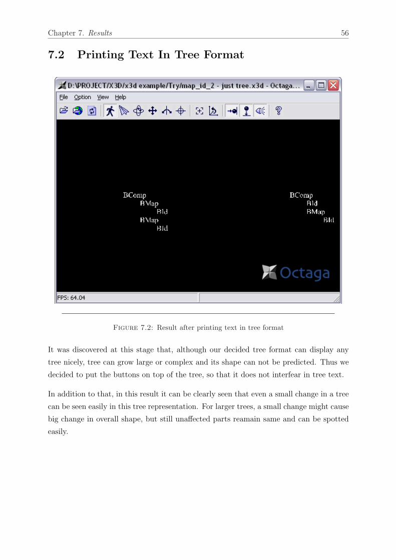
Chapter 7. Results 56
7.2 Printing Text In Tree Format
Figure 7.2: Result after printing text in tree format
It was discovered at this stage that, although our decided tree format can display any
tree nicely, tree can grow large or complex and its shape can not be predicted. Thus we
decided to put the buttons on top of the tree, so that it does not interfear in tree text.
In addition to that, in this result it can be clearly seen that even a small change in a tree
can be seen easily in this tree representation. For larger trees, a small change might cause
big change in overall shape, but still unaffected parts reamain same and can be spotted
easily.
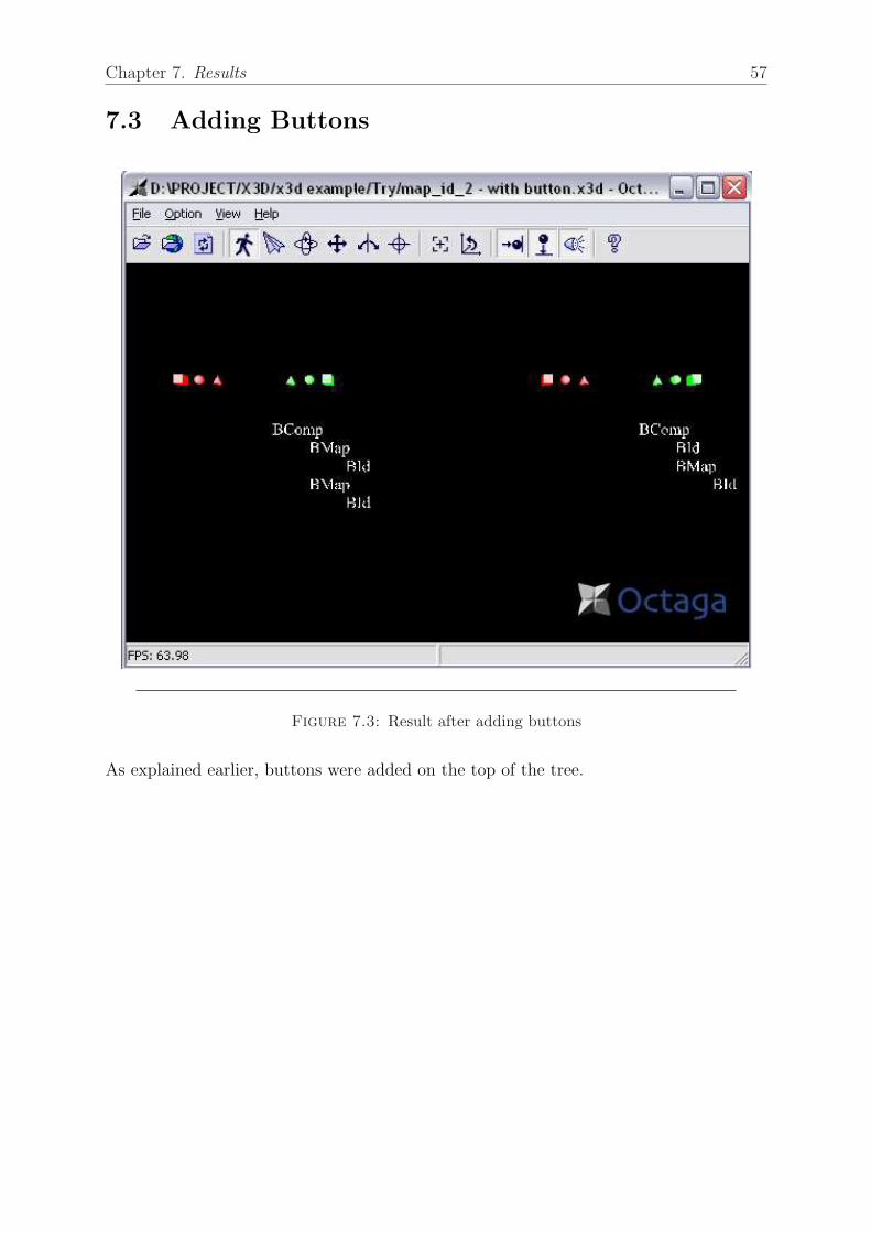
Chapter 7. Results 57
7.3 Adding Buttons
Figure 7.3: Result after adding buttons
As explained earlier, buttons were added on the top of the tree.
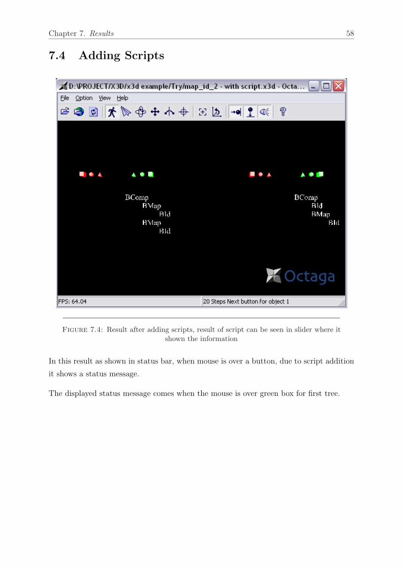
Chapter 7. Results 58
7.4 Adding Scripts
Figure 7.4: Result after adding scripts, result of script can be seen in slider where itshown the information
In this result as shown in status bar, when mouse is over a button, due to script addition
it shows a status message.
The displayed status message comes when the mouse is over green box for first tree.
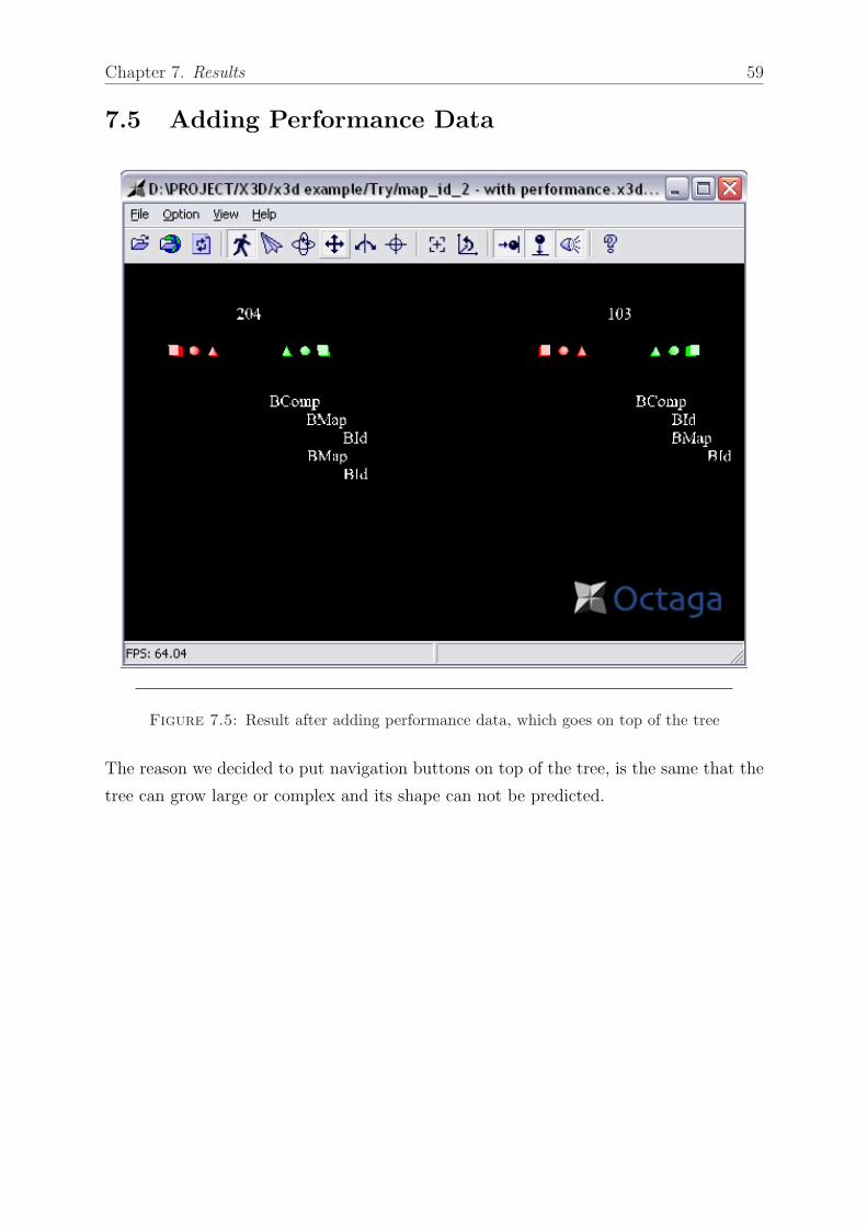
Chapter 7. Results 59
7.5 Adding Performance Data
Figure 7.5: Result after adding performance data, which goes on top of the tree
The reason we decided to put navigation buttons on top of the tree, is the same that the
tree can grow large or complex and its shape can not be predicted.
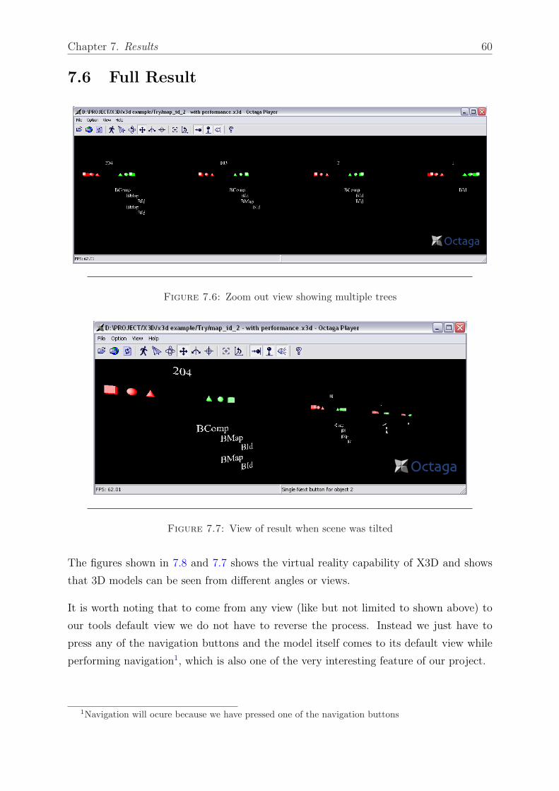
Chapter 7. Results 60
7.6 Full Result
Figure 7.6: Zoom out view showing multiple trees
Figure 7.7: View of result when scene was tilted
The figures shown in 7.8 and 7.7 shows the virtual reality capability of X3D and shows
that 3D models can be seen from different angles or views.
It is worth noting that to come from any view (like but not limited to shown above) to
our tools default view we do not have to reverse the process. Instead we just have to
press any of the navigation buttons and the model itself comes to its default view while
performing navigation1, which is also one of the very interesting feature of our project.
1Navigation will ocure because we have pressed one of the navigation buttons
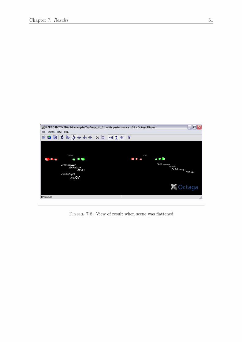
Chapter 7. Results 61
Figure 7.8: View of result when scene was flattened
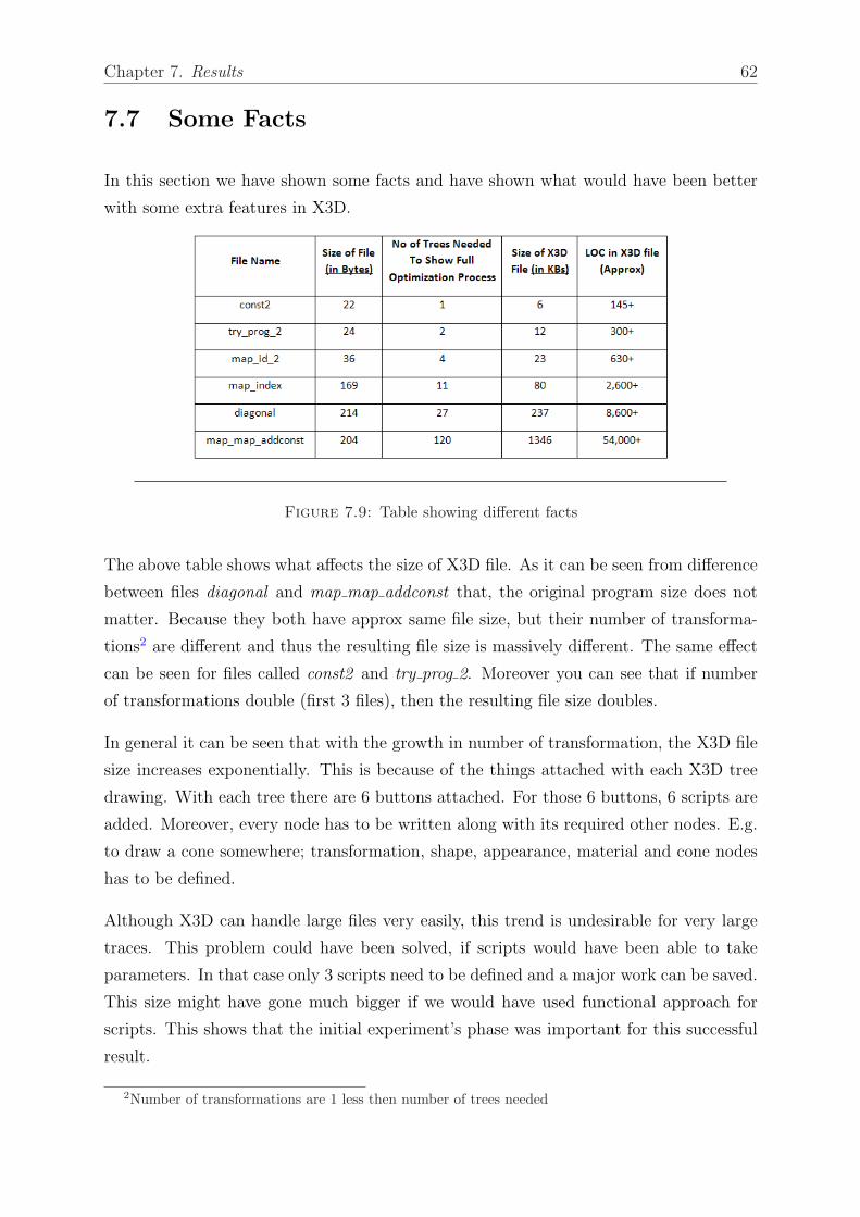
Chapter 7. Results 62
7.7 Some Facts
In this section we have shown some facts and have shown what would have been better
with some extra features in X3D.
Figure 7.9: Table showing different facts
The above table shows what affects the size of X3D file. As it can be seen from difference
between files diagonal and map map addconst that, the original program size does not
matter. Because they both have approx same file size, but their number of transforma-
tions2 are different and thus the resulting file size is massively different. The same effect
can be seen for files called const2 and try prog 2. Moreover you can see that if number
of transformations double (first 3 files), then the resulting file size doubles.
In general it can be seen that with the growth in number of transformation, the X3D file
size increases exponentially. This is because of the things attached with each X3D tree
drawing. With each tree there are 6 buttons attached. For those 6 buttons, 6 scripts are
added. Moreover, every node has to be written along with its required other nodes. E.g.
to draw a cone somewhere; transformation, shape, appearance, material and cone nodes
has to be defined.
Although X3D can handle large files very easily, this trend is undesirable for very large
traces. This problem could have been solved, if scripts would have been able to take
parameters. In that case only 3 scripts need to be defined and a major work can be saved.
This size might have gone much bigger if we would have used functional approach for
scripts. This shows that the initial experiment’s phase was important for this successful
result.
2Number of transformations are 1 less then number of trees needed

Chapter 8
Future Work
The current project can bring excellent improvement in BMF optimizer. But still with
advances in X3D and change in available technology some extensions can be added to
this project.
In future this visualizer can be extended to be more user-friendly. New interactive menus
can be added, options can be given to tweak the 3D model like changing number of
transformations a button should skip, changing the zoom level, changing the speed of
animation etc. This all can be also be done runtime.
There is also possibility to show 3D graph which can display various performance figures
and by clicking on any individual point it can show the AST at that time.
Along with performance data, name of applied rule can also be shown in 3d model. A
hot spot in AST, where recent change has occurred, can also be distinguished by some
mechanism for faster understanding of transformation.
Currently there is a limitation in X3D about how many children a node can handle. This
limit was more than enough for current project goals, but while extending the project in
future, this limitation should also be considered and may need upgrade. Moreover, with
some more advances in X3D, time based animation can be implemented which can be
more useful.
The movement and navigation is good at this point but it can be made spectacular with
auto zooming in and out (as per the size of tree), a longer navigation (like 500 trees) should
be done at faster pace than a smaller navigation (like 5 trees) to keep the navigation time
relatively consistent. These features does not add any major functionality but it gives
spectacular view.
63
Chapter 9
Conclusion
The BMF optimizer is very efficient for program optimization. Obscurity resulting from
very high number of transformations is a bottleneck in its evolution. To break this
obscurity we have taken the approach to display all transformations, in AST format, in a
3D model which displays all required information. It is also possible to navigate through
long lists of transformations with user interaction. Due to this work, It can be checked that
which rule is performing better under one type of circumstances, which under another. It
can also be discovered, why any particular rule is not performing well. It is also possible
to verify that no rule under any circumstances breaks the code and leads into unstable
solution. This is a major helping hand in evolution of the optimizer. X3D, though in its
development phase, is a very good tool to create 3D models. It combines some desirable
features like open standard software, user interactivity, animation, scripting, good 3D
modeling, etc. all in one tool. Overall we have found that, X3D can create sophisticated
3D models simply and have flexibility and accessibility for novice to expert users. Last
but not the least, this work has opened a new dimension in the way BMF optimizer
evolves and the same strategy, to visualize the internal process, can be used for other
optimizers or compilers as well.
64
Appendix A
X3D Syntax File
module basic_x3d
imports x3d_literals
exports
sorts Scene Viewpoint Transform Scenecomponent Shape Shapecomponent
Appearance Text Polyline2D Material Group Groupcomponent
context-free syntax
{Scenecomponent ","}+ -> Scene {cons("Scene")}
"Viewpoint" Coord Coord Coord PosInt ->
Viewpoint {cons("Viewpoint")}
"Transform" Coord Coord Coord Group ->
Transform {cons("Transform")}
"Transform" Coord Coord Coord Shape ->
Transform {cons("Transform")}
Transform -> Scenecomponent
Viewpoint -> Scenecomponent
"Group" {Groupcomponent ","}+ -> Group {cons("Group")}
"Group" PosInt PosInt PosInt PosInt PosInt PosInt PosInt PosInt
{Groupcomponent ","}+ -> Group {cons("Group")}
"Shape" Appearance Shapecomponent ->
Shape {cons("Shape")}
"Shape" Shapecomponent -> Shape {cons("Shape")}
65

Appendix A. X3D Syntax File 66
Shape -> Groupcomponent
Transform -> Groupcomponent
"Text" String -> Text {cons("Text")}
Text -> Shapecomponent
"Polyline2D" Coord Coord Coord Coord ->
Polyline2D {cons("Polyline2D")}
Polyline2D -> Shapecomponent
"Appearance" Material -> Appearance {cons("Appearence")}
"Material" Intensity Intensity Intensity ->
Material {cons("Material")}
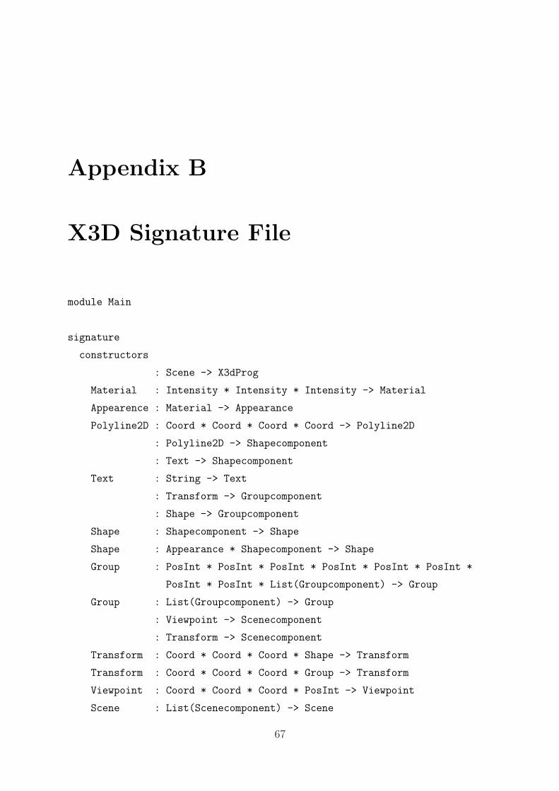
Appendix B
X3D Signature File
module Main
signature
constructors
: Scene -> X3dProg
Material : Intensity * Intensity * Intensity -> Material
Appearence : Material -> Appearance
Polyline2D : Coord * Coord * Coord * Coord -> Polyline2D
: Polyline2D -> Shapecomponent
: Text -> Shapecomponent
Text : String -> Text
: Transform -> Groupcomponent
: Shape -> Groupcomponent
Shape : Shapecomponent -> Shape
Shape : Appearance * Shapecomponent -> Shape
Group : PosInt * PosInt * PosInt * PosInt * PosInt * PosInt *
PosInt * PosInt * List(Groupcomponent) -> Group
Group : List(Groupcomponent) -> Group
: Viewpoint -> Scenecomponent
: Transform -> Scenecomponent
Transform : Coord * Coord * Coord * Shape -> Transform
Transform : Coord * Coord * Coord * Group -> Transform
Viewpoint : Coord * Coord * Coord * PosInt -> Viewpoint
Scene : List(Scenecomponent) -> Scene
67
Appendix B. X3D Signature File 68
: String -> String
: String -> PosInt
: String -> Intensity
: String -> Coord
signature
constructors
Some : a -> Option(a)
None : Option(a)
signature
constructors
Cons : a * List(a) -> List(a)
Nil : List(a)
Conc : List(a) * List(a) -> List(a)
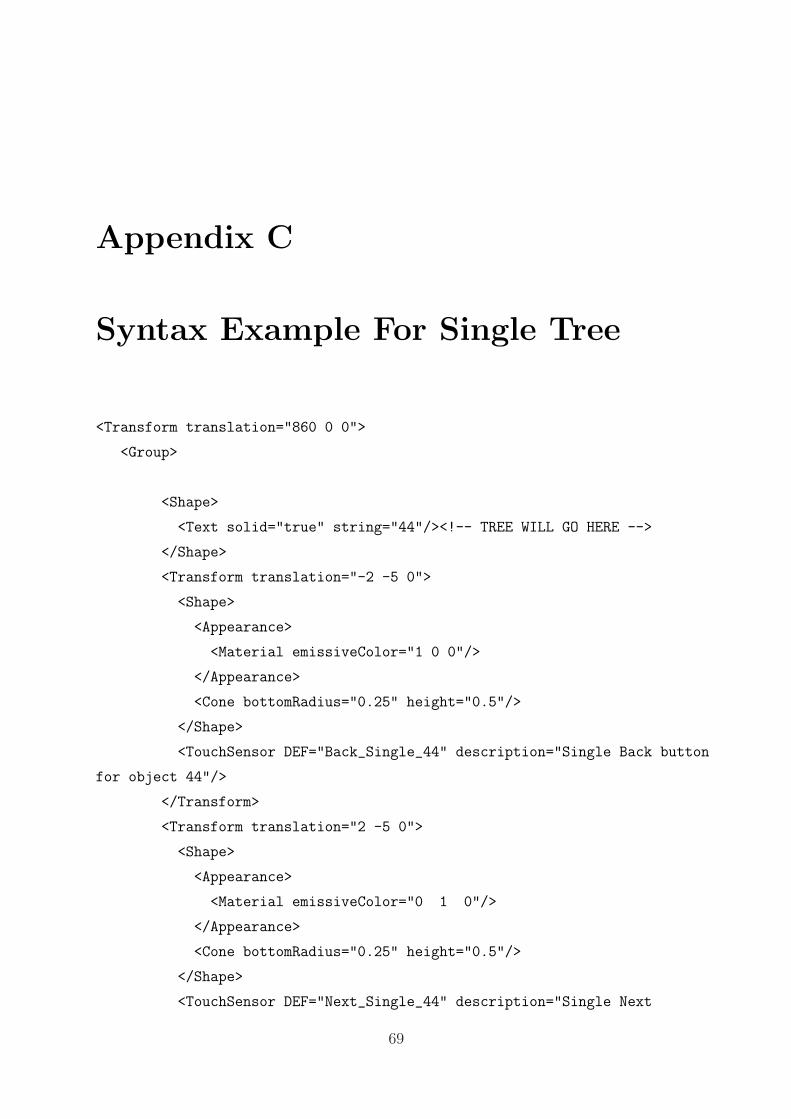
Appendix C
Syntax Example For Single Tree
<Transform translation="860 0 0">
<Group>
<Shape>
<Text solid="true" string="44"/><!-- TREE WILL GO HERE -->
</Shape>
<Transform translation="-2 -5 0">
<Shape>
<Appearance>
<Material emissiveColor="1 0 0"/>
</Appearance>
<Cone bottomRadius="0.25" height="0.5"/>
</Shape>
<TouchSensor DEF="Back_Single_44" description="Single Back button
for object 44"/>
</Transform>
<Transform translation="2 -5 0">
<Shape>
<Appearance>
<Material emissiveColor="0 1 0"/>
</Appearance>
<Cone bottomRadius="0.25" height="0.5"/>
</Shape>
<TouchSensor DEF="Next_Single_44" description="Single Next
69
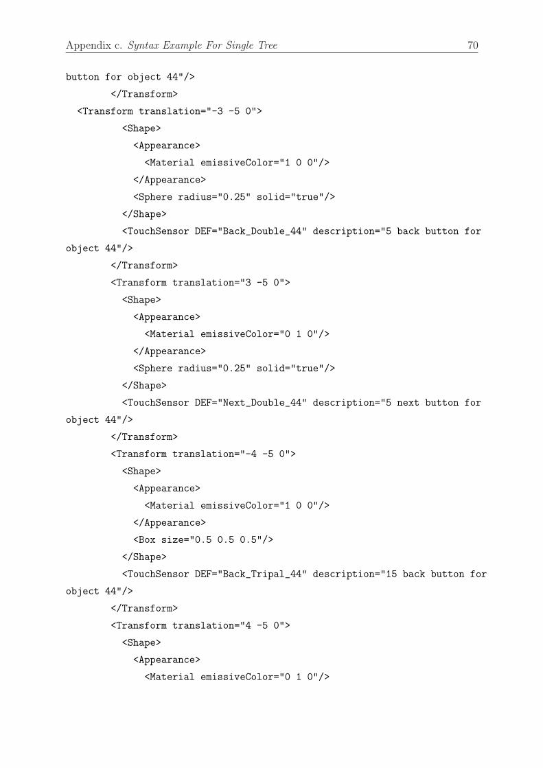
Appendix c. Syntax Example For Single Tree 70
button for object 44"/>
</Transform>
<Transform translation="-3 -5 0">
<Shape>
<Appearance>
<Material emissiveColor="1 0 0"/>
</Appearance>
<Sphere radius="0.25" solid="true"/>
</Shape>
<TouchSensor DEF="Back_Double_44" description="5 back button for
object 44"/>
</Transform>
<Transform translation="3 -5 0">
<Shape>
<Appearance>
<Material emissiveColor="0 1 0"/>
</Appearance>
<Sphere radius="0.25" solid="true"/>
</Shape>
<TouchSensor DEF="Next_Double_44" description="5 next button for
object 44"/>
</Transform>
<Transform translation="-4 -5 0">
<Shape>
<Appearance>
<Material emissiveColor="1 0 0"/>
</Appearance>
<Box size="0.5 0.5 0.5"/>
</Shape>
<TouchSensor DEF="Back_Tripal_44" description="15 back button for
object 44"/>
</Transform>
<Transform translation="4 -5 0">
<Shape>
<Appearance>
<Material emissiveColor="0 1 0"/>
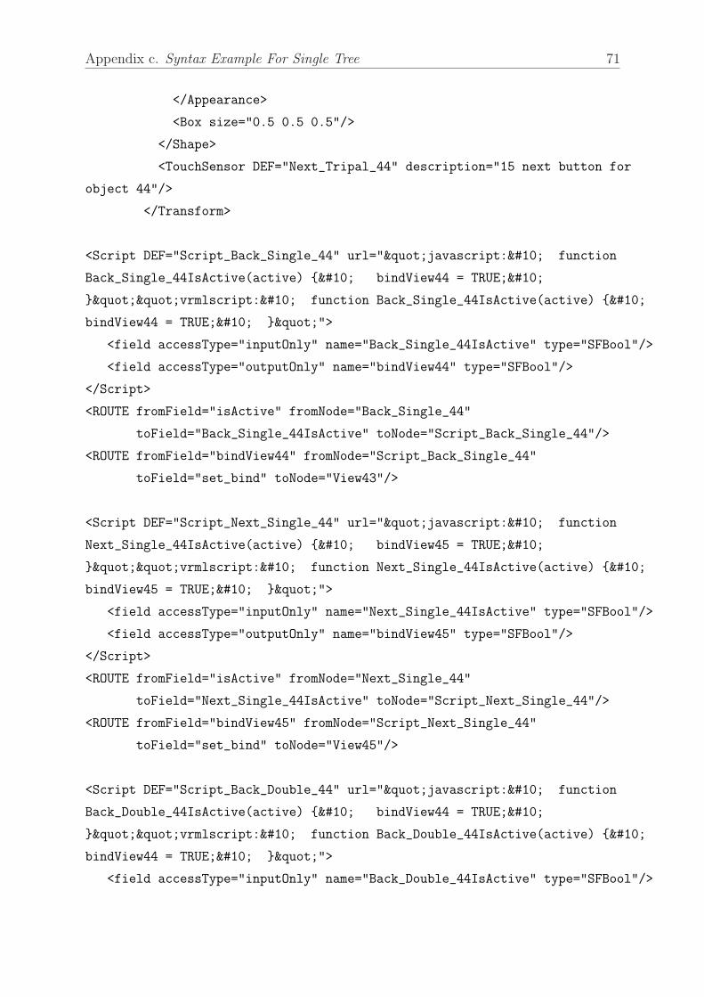
Appendix c. Syntax Example For Single Tree 71
</Appearance>
<Box size="0.5 0.5 0.5"/>
</Shape>
<TouchSensor DEF="Next_Tripal_44" description="15 next button for
object 44"/>
</Transform>
<Script DEF="Script_Back_Single_44" url=""javascript: function
Back_Single_44IsActive(active) { bindView44 = TRUE;
}""vrmlscript: function Back_Single_44IsActive(active) {
bindView44 = TRUE; }"">
<field accessType="inputOnly" name="Back_Single_44IsActive" type="SFBool"/>
<field accessType="outputOnly" name="bindView44" type="SFBool"/>
</Script>
<ROUTE fromField="isActive" fromNode="Back_Single_44"
toField="Back_Single_44IsActive" toNode="Script_Back_Single_44"/>
<ROUTE fromField="bindView44" fromNode="Script_Back_Single_44"
toField="set_bind" toNode="View43"/>
<Script DEF="Script_Next_Single_44" url=""javascript: function
Next_Single_44IsActive(active) { bindView45 = TRUE;
}""vrmlscript: function Next_Single_44IsActive(active) {
bindView45 = TRUE; }"">
<field accessType="inputOnly" name="Next_Single_44IsActive" type="SFBool"/>
<field accessType="outputOnly" name="bindView45" type="SFBool"/>
</Script>
<ROUTE fromField="isActive" fromNode="Next_Single_44"
toField="Next_Single_44IsActive" toNode="Script_Next_Single_44"/>
<ROUTE fromField="bindView45" fromNode="Script_Next_Single_44"
toField="set_bind" toNode="View45"/>
<Script DEF="Script_Back_Double_44" url=""javascript: function
Back_Double_44IsActive(active) { bindView44 = TRUE;
}""vrmlscript: function Back_Double_44IsActive(active) {
bindView44 = TRUE; }"">
<field accessType="inputOnly" name="Back_Double_44IsActive" type="SFBool"/>
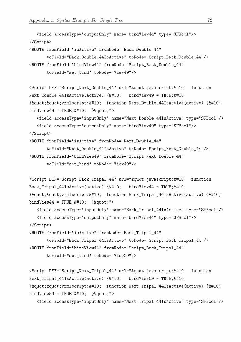
Appendix c. Syntax Example For Single Tree 72
<field accessType="outputOnly" name="bindView44" type="SFBool"/>
</Script>
<ROUTE fromField="isActive" fromNode="Back_Double_44"
toField="Back_Double_44IsActive" toNode="Script_Back_Double_44"/>
<ROUTE fromField="bindView44" fromNode="Script_Back_Double_44"
toField="set_bind" toNode="View49"/>
<Script DEF="Script_Next_Double_44" url=""javascript: function
Next_Double_44IsActive(active) { bindView49 = TRUE;
}""vrmlscript: function Next_Double_44IsActive(active) {
bindView49 = TRUE; }"">
<field accessType="inputOnly" name="Next_Double_44IsActive" type="SFBool"/>
<field accessType="outputOnly" name="bindView49" type="SFBool"/>
</Script>
<ROUTE fromField="isActive" fromNode="Next_Double_44"
toField="Next_Double_44IsActive" toNode="Script_Next_Double_44"/>
<ROUTE fromField="bindView49" fromNode="Script_Next_Double_44"
toField="set_bind" toNode="View49"/>
<Script DEF="Script_Back_Tripal_44" url=""javascript: function
Back_Tripal_44IsActive(active) { bindView44 = TRUE;
}""vrmlscript: function Back_Tripal_44IsActive(active) {
bindView44 = TRUE; }"">
<field accessType="inputOnly" name="Back_Tripal_44IsActive" type="SFBool"/>
<field accessType="outputOnly" name="bindView44" type="SFBool"/>
</Script>
<ROUTE fromField="isActive" fromNode="Back_Tripal_44"
toField="Back_Tripal_44IsActive" toNode="Script_Back_Tripal_44"/>
<ROUTE fromField="bindView44" fromNode="Script_Back_Tripal_44"
toField="set_bind" toNode="View29"/>
<Script DEF="Script_Next_Tripal_44" url=""javascript: function
Next_Tripal_44IsActive(active) { bindView59 = TRUE;
}""vrmlscript: function Next_Tripal_44IsActive(active) {
bindView59 = TRUE; }"">
<field accessType="inputOnly" name="Next_Tripal_44IsActive" type="SFBool"/>

Appendix c. Syntax Example For Single Tree 73
<field accessType="outputOnly" name="bindView59" type="SFBool"/>
</Script>
<ROUTE fromField="isActive" fromNode="Next_Tripal_44"
toField="Next_Tripal_44IsActive" toNode="Script_Next_Tripal_44"/>
<ROUTE fromField="bindView59" fromNode="Script_Next_Tripal_44"
toField="set_bind" toNode="View59"/>
</Group>
</Transform>
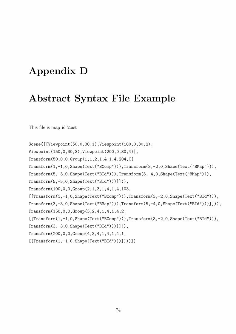
Appendix D
Abstract Syntax File Example
This file is map id 2.ast
Scene([[Viewpoint(50,0,30,1),Viewpoint(100,0,30,2),
Viewpoint(150,0,30,3),Viewpoint(200,0,30,4)],
Transform(50,0,0,Group(1,1,2,1,4,1,4,204,[[
Transform(1,-1,0,Shape(Text("BComp"))),Transform(3,-2,0,Shape(Text("BMap"))),
Transform(5,-3,0,Shape(Text("BId"))),Transform(3,-4,0,Shape(Text("BMap"))),
Transform(5,-5,0,Shape(Text("BId")))]])),
Transform(100,0,0,Group(2,1,3,1,4,1,4,103,
[[Transform(1,-1,0,Shape(Text("BComp"))),Transform(3,-2,0,Shape(Text("BId"))),
Transform(3,-3,0,Shape(Text("BMap"))),Transform(5,-4,0,Shape(Text("BId")))]])),
Transform(150,0,0,Group(3,2,4,1,4,1,4,2,
[[Transform(1,-1,0,Shape(Text("BComp"))),Transform(3,-2,0,Shape(Text("BId"))),
Transform(3,-3,0,Shape(Text("BId")))]])),
Transform(200,0,0,Group(4,3,4,1,4,1,4,1,
[[Transform(1,-1,0,Shape(Text("BId")))]]))])
74

Appendix E
Pretty Printing File
[
Scene -- H["<?xml version=\"1.0\" encoding=\"UTF-8\"?>
\n<!DOCTYPE X3D PUBLIC
\"http://www.web3d.org/specifications/x3d-3.1.dtd\"
\"file:///www.web3d.org/TaskGroups/x3d/translation/x3d-3.1.dtd\">
\n<X3D profile=\"Immersive\" version=\"3.1\"
xmlns:xsd=\"http://www.w3.org/2001/XMLSchema-instance\"
xsd:noNamespaceSchemaLocation=
\"http://www.web3d.org/specifications/x3d-3.1.xsd\">"]
"<Scene>"
_1
"\n\n </Scene>"
"\n</X3D>",
Scene.1:iter-sep -- _1 KW["\n"],
Viewpoint -- H hs=0[KW["\n<Viewpoint"]
" DEF=\"View"
_4
"\" description=\"view object"
_4
"\" position=\""]
_1 _2 _3
"\"/>",
75
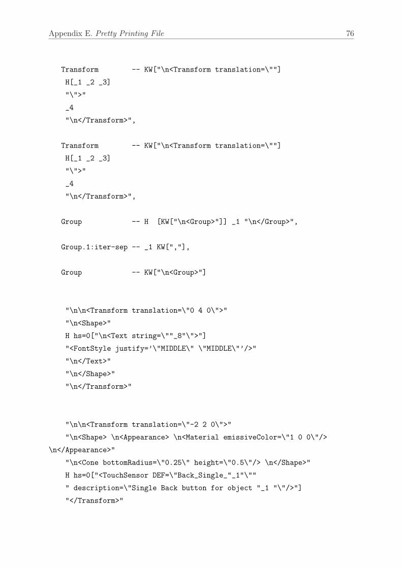
Appendix E. Pretty Printing File 76
Transform -- KW["\n<Transform translation=\""]
H[_1 _2 _3]
"\">"
_4
"\n</Transform>",
Transform -- KW["\n<Transform translation=\""]
H[_1 _2 _3]
"\">"
_4
"\n</Transform>",
Group -- H [KW["\n<Group>"]] _1 "\n</Group>",
Group.1:iter-sep -- _1 KW[","],
Group -- KW["\n<Group>"]
"\n\n<Transform translation=\"0 4 0\">"
"\n<Shape>"
H hs=0["\n<Text string=\""_8"\">"]
"<FontStyle justify=’\"MIDDLE\" \"MIDDLE\"’/>"
"\n</Text>"
"\n</Shape>"
"\n</Transform>"
"\n\n<Transform translation=\"-2 2 0\">"
"\n<Shape> \n<Appearance> \n<Material emissiveColor=\"1 0 0\"/>
\n</Appearance>"
"\n<Cone bottomRadius=\"0.25\" height=\"0.5\"/> \n</Shape>"
H hs=0["<TouchSensor DEF=\"Back_Single_"_1"\""
" description=\"Single Back button for object "_1 "\"/>"]
"</Transform>"
Appendix E. Pretty Printing File 77
"\n\n<Transform translation=\"2 2 0\">"
"\n<Shape> \n<Appearance> \n<Material emissiveColor=\"0 1 0\"/>
\n</Appearance>"
"\n<Cone bottomRadius=\"0.25\" height=\"0.5\"/> \n</Shape>"
H hs=0["<TouchSensor DEF=\"Next_Single_"_1"\""
" description=\"Single Next button for object "_1 "\"/>"]
"</Transform>"
"\n\n<Transform translation=\"-3 2 0\">"
"\n<Shape> \n<Appearance> \n<Material emissiveColor=\"1 0 0\"/>
\n</Appearance>"
"\n<Sphere radius=\"0.25\" solid=\"true\"/> \n</Shape>"
H hs=0["<TouchSensor DEF=\"Back_Double_"_1"\""
" description=\"10 Steps Back button for object "_1 "\"/>"]
"</Transform>"
"\n\n<Transform translation=\"3 2 0\">"
"\n<Shape> \n<Appearance> \n<Material emissiveColor=\"0 1 0\"/>
\n</Appearance>"
"\n<Sphere radius=\"0.25\" solid=\"true\"/> \n</Shape>"
H hs=0["<TouchSensor DEF=\"Next_Double_"_1"\""
" description=\"10 Steps Next button for object "_1 "\"/>"]
"</Transform>"
"\n\n<Transform translation=\"-4 2 0\">"
"\n<Shape> \n<Appearance> \n<Material emissiveColor=\"1 0 0\"/>
\n</Appearance>"
"\n<Box size=\"0.5 0.5 0.5\" solid=\"true\"/> \n</Shape>"
H hs=0["<TouchSensor DEF=\"Back_Triple_"_1"\""
" description=\"20 Steps Back button for object "_1 "\"/>"]
"</Transform>"
"\n\n<Transform translation=\"4 2 0\">"
"\n<Shape> \n<Appearance> \n<Material emissiveColor=\"0 1 0\"/>
\n</Appearance>"
Appendix E. Pretty Printing File 78
"\n<Box size=\"0.5 0.5 0.5\" solid=\"true\"/> \n</Shape>"
H hs=0["<TouchSensor DEF=\"Next_Triple_"_1"\""
" description=\"20 Steps Next button for object "_1 "\"/>"]
"</Transform>"
"\n" _9 "\n\n"
H hs=0[
"\n<Script DEF=\"Script_Back_Single_" _1 "\""
" url=\""javascript: "
" function Back_Single_" _1 "IsActive(active)"
" { bindView" _1 "= TRUE; }""vrmlscript: "
" function Back_Single_" _1 "IsActive(active)"
" { bindView" _1 " = TRUE; }"\"> "
"\n<field accessType=\"inputOnly\" name=
\"Back_Single_"_1"IsActive\" type=\"SFBool\"/>"
"\n<field accessType=\"outputOnly\" name=
\"bindView"_1"\" type=\"SFBool\"/>"
"\n</Script>"
"\n<ROUTE fromField=\"isActive\" fromNode=\"Back_Single_"_1"\""
"\n toField=\"Back_Single_"_1"IsActive\""
" toNode=\"Script_Back_Single_"_1"\"/>"
"\n<ROUTE fromField=\"bindView"_1"\" fromNode=\"Script_Back_Single_"_1"\" "
"\n toField=\"set_bind\""
" toNode=\"View"_2"\"/>"
"\n\n<Script DEF=\"Script_Next_Single_"_1"\""
" url=\""javascript: "
" function Next_Single_"_1"IsActive(active)"
" { bindView"_3" = TRUE; }""vrmlscript: "
" function Next_Single_"_1"IsActive(active)"
" { bindView"_3" = TRUE; }"\">"
Appendix E. Pretty Printing File 79
"\n<field accessType=\"inputOnly\" name=\"Next_Single_"_1"IsActive\"
type=\"SFBool\"/>"
"\n<field accessType=\"outputOnly\" name=\"bindView"_3"\"
type=\"SFBool\"/>"
"\n</Script>"
"\n<ROUTE fromField=\"isActive\" fromNode=\"Next_Single_"_1"\""
"\n toField=\"Next_Single_"_1"IsActive\""
" toNode=\"Script_Next_Single_"_1"\"/>"
"\n<ROUTE fromField=\"bindView"_3"\" fromNode=\"Script_Next_Single_"_1"\""
"\n toField=\"set_bind\""
" toNode=\"View"_3"\"/>"
]
H hs=0[
"\n<Script DEF=\"Script_Back_Double_" _1 "\""
" url=\""javascript: "
" function Back_Double_" _1 "IsActive(active)"
" { bindView" _1 "= TRUE; }""vrmlscript: "
" function Back_Double_" _1 "IsActive(active)"
" { bindView" _1 " = TRUE; }"\"> "
"\n<field accessType=\"inputOnly\" name=
\"Back_Double_"_1"IsActive\" type=\"SFBool\"/>"
"\n<field accessType=\"outputOnly\" name=
\"bindView"_1"\" type=\"SFBool\"/>"
"\n</Script>"
"\n<ROUTE fromField=\"isActive\" fromNode=\"Back_Double_"_1"\""
"\n toField=\"Back_Double_"_1"IsActive\""
" toNode=\"Script_Back_Double_"_1"\"/>"
"\n<ROUTE fromField=\"bindView"_1"\" fromNode=\"Script_Back_Double_"_1"\" "
"\n toField=\"set_bind\""
" toNode=\"View"_4"\"/>"
Appendix E. Pretty Printing File 80
"\n\n<Script DEF=\"Script_Next_Double_"_1"\""
" url=\""javascript: "
" function Next_Double_"_1"IsActive(active)"
" { bindView"_5" = TRUE; }""vrmlscript: "
" function Next_Double_"_1"IsActive(active)"
" { bindView"_5" = TRUE; }"\">"
"\n<field accessType=\"inputOnly\" name=\"Next_Double_"_1"IsActive\"
type=\"SFBool\"/>"
"\n<field accessType=\"outputOnly\" name=\"bindView"_5"\"
type=\"SFBool\"/>"
"\n</Script>"
"\n<ROUTE fromField=\"isActive\" fromNode=\"Next_Double_"_1"\""
"\n toField=\"Next_Double_"_1"IsActive\""
" toNode=\"Script_Next_Double_"_1"\"/>"
"\n<ROUTE fromField=\"bindView"_5"\" fromNode=\"Script_Next_Double_"_1"\""
"\n toField=\"set_bind\""
" toNode=\"View"_5"\"/>"
]
H hs=0[
"\n<Script DEF=\"Script_Back_Triple_" _1 "\""
" url=\""javascript: "
" function Back_Triple_" _1 "IsActive(active)"
" { bindView" _1 "= TRUE; }""vrmlscript: "
" function Back_Triple_" _1 "IsActive(active)"
" { bindView" _1 " = TRUE; }"\"> "
"\n<field accessType=\"inputOnly\" name=
\"Back_Triple_"_1"IsActive\" type=\"SFBool\"/>"
"\n<field accessType=\"outputOnly\" name=
\"bindView"_1"\" type=\"SFBool\"/>"
"\n</Script>"
Appendix E. Pretty Printing File 81
"\n<ROUTE fromField=\"isActive\" fromNode=\"Back_Triple_"_1"\""
"\n toField=\"Back_Triple_"_1"IsActive\""
" toNode=\"Script_Back_Triple_"_1"\"/>"
"\n<ROUTE fromField=\"bindView"_1"\" fromNode=\"Script_Back_Triple_"_1"\" "
"\n toField=\"set_bind\""
" toNode=\"View"_6"\"/>"
"\n\n<Script DEF=\"Script_Next_Triple_"_1"\""
" url=\""javascript: "
" function Next_Triple_"_1"IsActive(active)"
" { bindView"_7" = TRUE; }""vrmlscript: "
" function Next_Triple_"_1"IsActive(active)"
" { bindView"_7" = TRUE; }"\">"
"\n<field accessType=\"inputOnly\" name=\"Next_Triple_"_1"IsActive\"
type=\"SFBool\"/>"
"\n<field accessType=\"outputOnly\" name=\"bindView"_7"\"
type=\"SFBool\"/>"
"\n</Script>"
"\n<ROUTE fromField=\"isActive\" fromNode=\"Next_Triple_"_1"\""
"\n toField=\"Next_Triple_"_1"IsActive\""
" toNode=\"Script_Next_Triple_"_1"\"/>"
"\n<ROUTE fromField=\"bindView"_7"\" fromNode=\"Script_Next_Triple_"_1"\""
"\n toField=\"set_bind\""
" toNode=\"View"_7"\"/>"
]
"\n\n</Group>",
Group.2:iter-sep -- _1 KW[","],
Shape -- KW["<Shape>"]
H[_1 _2]
Appendix E. Pretty Printing File 82
"\n</Shape>",
Shape -- KW["\n<Shape>"]
_1
"\n</Shape>",
Text -- H hs=0[KW["\n<Text string=\""]
_1
"\" />"],
Polyline2D -- KW["<Polyline2D lineSegments=\""]
H[_1 _2 _3 _4]
"\"/>",
Cone -- KW["<Cone bottomRadius=\"0.25\" height=\"0.5\" /> "],
Appearence -- KW["\n<Appearance>"]
_1
"\n</Appearance>",
Material -- KW[ "\n<Material emissiveColor=\"" ]
H[_1 _2 _3]
"\"/>"
]

Bibliography
[1] http://releases.strategoxt.org/strategoxt-manual/unstable/manual/chunk-
chapter/tutorial-software-transformation-systems.html
[2] http://releases.strategoxt.org/strategoxt-manual/unstable/manual/chunk-
chapter/rules-and-strategies.html
[3] Stratego/XT 0.16: Components for Transformation Systems,
Martin Bravenboer, Karl Trygve Kalleberg, Rob Vermaas, Eelco Visser
http://igitur-archive.library.uu.nl/math/2007-1127-200705/bravenboer 05 strategoxt016components.pdf
[4] X3D: Extensible 3D Graphics for Web Authors,
Brutzman, Don; Daly, Leonard,
[5] http://www.web3d.org/about/overview/
[6] http://www.web3d.org/x3d/workgroups/cad/
[7] The Simulation and Visualization of Parallel BMF Code
Paul Martinaitis
http://www.cs.adelaide.edu.au/ brad/students/paulm.pdf Nov-98
[8] http://releases.strategoxt.org/strategoxt-manual/unstable/manual/chunk-
chapter/stratego-terms.html
[9] http://www.adobe.com/products/flashlite/
[10] http://www.adobe.com/products/player census/flashplayer/version penetration.html
[11] http://www.adobe.com/products/flash/
[12] http://tuesdaycreative.vox.com/library/post/the-top-ten-open-source-actionscript-
tools.html
[13] http://www.adobe.com/products/flash/features/allfeatures/
83

Bibliography 84
[14] http://www.povray.org/resources/
[15] http://www.blender.org/features-gallery/features/
[16] http://usa.autodesk.com/adsk/servlet/index?siteID=123112&id=8108755
[17] http://www.adobe.com/devnet/acrobat3d/
[18] Strategic Rewriting for Simplified Optimisation of Point-Free Programs
Brad Alexander
[19] 3D Graphics on the Internet
Hans J. Wolters
http://www.hpl.hp.co.uk/research/mmsl/presentations/3d/3dweb.pdf
[20] http://releases.strategoxt.org/strategoxt-manual/unstable/manual/chunk-
chapter/ref-ast2text.html
[21] http://www.web3d.org/x3d/specifications/ISO-IEC-19775-
X3DAbstractSpecification/Part01/components/interp.html
[22] http://www.web3d.org/x3d/specifications/ISO-IEC-19775-
X3DAbstractSpecification/Part01/components/scripting.html
[23] http://www.web3d.org/x3d/specifications/ISO-IEC-19775-
X3DAbstractSpecification/Part01/components/pointingsensor.html
[24] http://releases.strategoxt.org/strategoxt-manual/unstable/manual/chunk-
chapter/stratego-traversal-strategies.html
[25] http://www.graphviz.org/
[26] SWF File Format Specification, Version 9
Adobe
http://www.adobe.com/devnet/swf/pdf/swf file format spec v9.pdf
[27] http://www.program-transformation.org/Stratego/
[28] http://sketchup.google.com/product/gsu.html