Visual tracking with L1-Grassmann manifold modeling · Visual Tracking with L1-Grassmann Manifold Modeling Dimitris G. Chachlakis a, Panos P. Markopoulos a, Raj. J. Muchhala b, and

Visual Tracking with L1-Grassmann Manifold Modeling

Dimitris G. Chachlakisa, Panos P. Markopoulosa, Raj. J. Muchhalab, and Andreas Savakisb

aDepartment of Electrical and Microelectronic Engineering, Rochester Institute of Technology,Rochester, NY 14623, USA

bDepartment of Computer Engineering, Rochester Institute of Technology, Rochester, NY14623, USA

ABSTRACT

We present a novel method for robust tracking in video frame sequences via L1-Grassmann manifolds. Theproposed method represents adaptively the target as a point on the Grassmann manifold, calculated by means ofL1-norm Principal-Component Analysis (L1-PCA). For this purpose, an efficient algorithm for adaptive L1-PCAis presented. Our experimental studies illustrate that the presented tracking method, leveraging the outlierresistance of L1-PCA, demonstrates robustness against target occlusions and illumination variations.

Keywords: Grassmann manifolds, L1-norm Principal-Component Analysis, occlusions, outliers, visual tracking.

1. INTRODUCTION

In the field of computer vision, visual tracking is extensively used for, e.g., surveillance and human behavioranalysis.1–4 In recent years, several methods have utilized deep learning features.5–8 In approaches utilizingsubspace-based tracking, Shirazi et al.9 proposed the Affine Subspace Tracker (AST), a novel tracking methodthat introduced the concept of visual tracking on Grassmann manifolds. AST represents the tracked object(target) as a point on the Grassmann manifold, calculated by means of standard Principal-Component Analysis(PCA). AST demonstrated that tracking on Grassmann manifolds can handle effectively a number of commonchallenges such as target-appearance variations. Ross et al.10 had previously presented a tracking methodthat relies on incrementally learned low-dimensional subspaces that adapt efficiently to changes in the appear-ance of the target. Zhang et al.11 introduced a successful tracking approach based on manifold learning withtwo-dimensional Local Preserving Projections (2DLPP). All the above methods have made a clear case on howprincipal-component representations can capture appearance changes of the target, while preserving local struc-tural information. In addition, in the past decades, extended research effort has been invested in developingtracking schemes that can handle effectively target occlusions and illumination variations. Despite their successagainst pose and shape changes of the target and illumination variations, currently existing Grassmann-basedvisual tracking methods do not emphasize on handling occlusions and motion blur.

In this work, we develop a novel visual tracking method based on Grassmann manifold representations.However, in contrast to all previous approaches, we propose to calculate Grassmann manifold points by means ofL1-norm Principal-Component Analysis (L1-PCA).12–18 We refer to those points as L1-Grassmann points and tothe proposed tracker as the L1-Grassmann tracker. Leveraging the well-documented outlier-resistance of L1-PCA,in sharp contrast to the sensitivity of standard PCA, the proposed method exhibits robustness against both targetocclusions by background components and illumination changes, offering overall high tracking performance. Inthe core of the proposed method lies a newly proposed algorithm for online L1-PCA adaptation.

The remainder of this paper is organized as follows. In Section 2, we offer a brief introduction to L1-PCAand introduce our L1-PCA adaptation algorithm. In Section 3, we present in detail the proposed L1-Grassmann

Further author information: (Send correspondence to A.S.)D.G.C.: E-mail: [email protected], Telephone: +1 585 733 9355P.P.M.: E-mail: [email protected], Telephone: +1 585 475 7917R.J.M.: E-mail: [email protected].: E-mail: [email protected], Telephone: +1 585 475 5651

Compressive Sensing VI: From Diverse Modalities to Big Data Analytics, edited byFauzia Ahmad, Proc. of SPIE Vol. 10211, 1021102 · © 2017 SPIE

CCC code: 0277-786X/17/$18 · doi: 10.1117/12.2263691

Proc. of SPIE Vol. 10211 1021102-1

Downloaded From: http://proceedings.spiedigitallibrary.org/ on 07/17/2017 Terms of Use: http://spiedigitallibrary.org/ss/termsofuse.aspx

visual tracking methodology. In Section 4, we offer experimental studies that illustrate the L1-PCA-endowedrobustness of the proposed method against occlusions and illumination variations. Concluding remarks are drawnin Section 5.

2. ADAPTIVE L1-NORM PRINCIPAL-COMPONENT ANALYSIS

2.1 Background

Consider data matrix X = [x1,x2, . . . ,xN ] ∈ RD×N of rank d ≤ min{D,N}. Principal-Component Analysisseeks a K-dimensional subspace, spanned by some orthonormal basis Q ∈ RD×K ,Q>Q = IK , wherein data-presence is maximized. Quantifying data-presence as the total variance (sum of squared Euclidean norms) of thesubspace-projected points, PCA is traditionally formulated as

QL2 = arg maxQ∈RD×K ;Q>Q=IK

∥∥X>Q∥∥22, (1)

where ‖·‖2 returns the L2-norm (also known as Frobenius norm) of its matrix argument. Due to its formulation in(1), PCA is also commonly referred to as L2-PCA. The solution to (1) is given by the singular-value decomposition(SVD) of X, with QL2 consisting of the K highest-singular-value left-hand singular vectors of X. Despite itscelebrated performance when X consists of nominal or smoothly corrupted data points and its asymptoticoptimality under certain data distributions, L2-PCA is well known to suffer from severe sensitivity to outliers inX19 –i.e., to minority points in X that lie far from the nominal data subspace. The reason for this sensitivity

is the squared emphasis that the L2-PCA optimization metric∥∥X>Q

∥∥22

=∑N

i=1

∥∥x>i Q∥∥22

=∑N

i=1

∑Kl=1 |x>i ql|2

allocates to each and every datum, thus benefiting unfavorably peripheral, deviating points. To remedy theimpact of outliers, research efforts have recently steered toward L1-PCA,16 a robust PCA alternative that seeksto maximize the L1-norm of the projected data as

QL1 = arg maxQ∈RD×K ;Q>Q=IK

∥∥X>Q∥∥1, (2)

where∥∥X>Q

∥∥1

=∑N

i=1

∥∥x>i Q∥∥1

=∑N

i=1

∑Kl=1 |x>i ql|. L1-PCA has already demonstrated significant robust-

ness against outliers in a wide array of applications, including face recognition,20,21 image restoration,22 andbackground tracking.23 Markopoulos et al.16 provided a formal proof on the NP-hardness of L1-PCA(2) injointly N and D. Existing L1-PCA calculators include both approximate12,13,17,18 and, more recently, exactalgorithms.? The first of the two existing optimal algorithms has complexity O

(2NK

), for jointly asymptotic

N and D; the second optimal algorithm has complexity O(N (d−1)K+1

), when d = rank(X) is a constant with

respect to N . Subsequent to these optimal solvers, a new efficient algorithm for L1-PCA was proposed, based onoptimal single-bit flipping (L1-BF).14,15 L1-BF, has complexity O

(NDmin{N,D}+N2K2

(K2 + d

)), similar

to that of standard L2-PCA (SVD) and appropriate for applications where N and/or D are large. In addition,L1-BF has been shown to offer the exact L1-PCA solution with very high frequency, outperforming in generalall previously proposed approximate calculators. In view of the above, in this work we employ L1-BF for theproposed L1-Grassmann visual tracking method. A brief description of L1-BF follows.

2.2 L1-PCA via L1-BF

It was proven16 that L1-PCA in (2) can be solved via combinatorial optimization. Specifically, if

Bopt = arg maxB∈{±1}N×K

‖XB‖∗ , (3)

where the nuclear norm ‖ · ‖∗ returns the summation of the singular values of its argument, and XBopt svd=

UΣK×KVT , thenQL1 = UVT (4)

is an exact solution to (2). In view of the above, L1-BF approximates efficiently the solution to (3) by abinary matrix Bbf and then approximates the exact L1-PCs similarly to (4). Specifically, L1-BF is initialized at

Proc. of SPIE Vol. 10211 1021102-2


L1-BF Algorithm for L1-PCA // (Qbf ,Bbf)← L1-BF(X,K)

Input: Data matrix XD×N ; K ≤ rank(X)1: (U,Σ,V)← svd(X)

2: Bbf ← BF(X, sgn([V]:,11

>K),K

)3: (U,ΣK×K ,V)← svd(XBbf)

4: Qbf ← UV>

Output: Qbf , Bbf

Function B← BF(XD×N ,BN×K ,K)

1: ω ← K‖X[B]:,1‖22: while true (or terminate at NK iterations)4: for m ∈ {1, 2, . . . , N}, l ∈ {1, 2, . . . ,K}5: am,l ←

∥∥X(B− 2Bm,lem,Ne>l,K

)∥∥∗

6: end for10: (n, k)← argmax am,l

11: if ω < an,k, Bn,k ← −Bn,k, ω ← an,k

12: else, break13: Return B

Figure 1: The L1-BF algorithm14,15 that calculates/approximates the K L1-PCs of a rank-d data matrix XD×N .

some B(0) ∈ {±1}N×K and conducts a sequence of optimal single-bit-flipping iterations. Importantly, at everybit-flipping iteration the metric of (3) increases and, thus, the iterations converge in a finite number of steps(empirically, in the order of NK). Mathematically, at the t-th iteration step, L1-BF seeks the single bit theflipping (negation) of which would offer the highest increase to the metric (3) by solving

(n, k) = argmax(m,l)∈{1,2,...,N}×{1,2,...,K}

∥∥∥X(B(t−1)− 2B(t−1)m,l em,Ne>l,K)

∥∥∥∗, (5)

through exhaustive search in the size-NK feasibility set. Then, it flips the (n, k)-th entry of B(t−1) as

B(t) = B(t−1) − 2B(t−1)n,k en,Ne>k,K , (6)

where ej,J denotes the j-th column of the size-J identity matrix IJ . At the converging iteration tc, L1-BF returns

Bbf = B(tc) and approximates QL1 by Qbf = UV>, where UΣK×K

V>svd= XBbf, in accordance to (4). A detailed

pseudo-code for L1-BF is provided in Fig. 1.∗ MATLAB scripts for L1-BF14,15 and the optimal L1-PCA solvers16

are publicly available online.24

To demonstrate the outlier resistance of the L1-BF principal-component calculator, we present the following

line-fitting experiment. We generate N = 18 points from N(02,[25.5 5

5 1.5

])organized in data matrix X ∈

R2×18. In Fig. 2(a) we draw the K = 1 principal component (PC) of X calculated by means of L2-PCA (SVD)and L1-BF. Then, we create an outlier corrupted version of the same dataset, Xcor = [X, O] ∈ R2×21, byappending three outlier points in O ∈ R2×3, drawn from N (0, 100 I2). In Fig. 2(b), we plot the first PC ofXcor, calculated again by SVD and L1-BF. We observe that in the corruption-free case (Fig. 2(a)) both PCsspan almost perfectly the nominal maximum-variance direction. However, when the dataset is outlier-corrupted(Fig. 2(b)) the L2-PC is profoundly misled, while the L1-BF-calculated PC exhibits sturdy resistance againstthe outliers.

∗Experimental studies have shown that a successful initialization matrix B(0) that offers fast convergence to a nearoptimal solution is sgn(z)1>K ∈ {±1}N×K , where z ∈ RN is the highest-singular-value right-hand singular vector of X,1K is the all-ones vector of length K, and sgn(·) is the sign-operation function that returns the {±1}-sign of its argument(see line 2 in the pseudo-code of Fig. 1).

Proc. of SPIE Vol. 10211 1021102-3


-150 -100 -50 0 50 100 150

-200

-150

-100

-50

0

50

100

150

200

(a)

-150 -100 -50 0 50 100 150

-200

-150

-100

-50

0

50

100

150

200

(b)

Figure 2: Line-fitting with L2-PC (by SVD) and L1-PC (by L1-BF14,15), for (a) nominal and (b) outlier-corrupteddata.

Proposed L1-PCA Adaptation Algorithm // (Qnew,bf ,Bnew,bf)← A-L1-BF(Xnew,Bbf ,K)

Input: New data matrix Xnew ∈ RD×N ; K ≤ rank(Xnew); previous bit-matrix Bbf , corresponding to Qbf

1: Bnew,bf ← BF (X,Bbf,K)

2: (U,ΣK×K ,V)← svd(XBnew,bf)

3: Qnew,bf ← UV>

Output: Qnew,bf , Bnew,bf

Figure 3: Proposed algorithm for L1-PCA adaptation.

2.3 L1-PCA Adaptation

As shown in the following section, a core part of the proposed L1-Grassmann visual tracking method is theadaptation of the target-describing subspaces (or Grassmann manifold points). To that end, at this point, wepresent a simple but efficient method for L1-PCA adaptation.

Consider data matrix X ∈ RD×N and let Qbf ∈ RD×K carry its K L1-PCs, as returned by L1-BF togetherwith the associated bit-matrix Bbf∈{±1}N×K (see Fig. 1). Next, consider that the points in X that have index in

I ⊂ {1, 2, . . . , N}, with |I| = n < N , are substituted by some new points in Y ∈ RD×n (e.g., new measurements),resulting in the updated data matrix Xnew, such that

[Xnew]:,I = Y and [Xnew]:,Ic = [X]:,Ic (7)

where Ic = {1, 2, . . . , N} \ I. Our goal is to approximate fast the K L1-PCs of Xnew taking advantage of ourprior knowledge on Qbf and Bbf . Simplifying the successful adaptation scheme proposed recently by Pierantozziet al.,25 in this work we propose to calculate the K L1-PCs of Xbf,new by running single-bit-flipping iterationson Xnew, initialized at the previously found bit-matrix Bbf . Denoting by Bbf,new the converging point of thesebit-flipping iterations,

Bbf,new ← BF(Xnew,Bbf ,K) (8)

(see Fig. 1), we approximate the K L1-PCs of Xnew by Qbf,new = UV>, where UΣK×KV>svd= XnewBbf,new.

The proposed L1-PCA adaptation scheme is presented in detail in the pseudo-code of Fig. 3.

3. PROPOSED L1-GRASSMANN TRACKER

We consider a grayscale video sequence that consists of N frames of height h and width w. A moving target ofinterest appears throughout the entire sequence, with the possibility of its partial or full occlusion in some of the

Proc. of SPIE Vol. 10211 1021102-4


frames. The goal of the proposed visual tracker is to locate accurately as possible the target in each video frame,scanning them sequentially from the first to the last one. Specifically, the tracker wishes to identify in eachframe a rectangular area in the size of the target that best encompasses it. For simplicity, we assume that thesize of the target does not change significantly throughout the video and that the height and width dimensionsof the rectangle that best fits the target, say ht < h and wt < w, respectively, are fixed and a priori known. Ahigh-level overview of the proposed tracking method follows.

The proposed L1-Grassmann tracker represents adaptively the target by a single point on a Grassmannmanifold, calculated by means of L1-BF. The Grassmann manifold Gr(a, b) is the space of all a-dimensionallinear subspaces in Rb, for a < b –i.e., an a-dimensional subspace in Rb can be represented as a single pointin Gr(a, b). When a new video frame arrives, the tracker identifies within it several candidate target locations;then, for each candidate location, it calculates by means of L1-BF a point to represent it on the same Grassmannmanifold. Tracking then is conducted by selecting the candidate-location that lies closest to the trained targeton the Grassmann manifold. Periodically, the proposed method uses the newly tracked target location to updatethe target-representing manifold point, thus accounting for changes in the target’s appearance (e.g., pose, shape,illumination). In the sequel, we present in detail the proposed method discussing separately the adaptive trainingand tracking procedures.

3.1 Adaptive Target-point Training

Initialization. We assume that the tracker knows (almost) perfectly the target location in the first m << Nframes. That is, the target knows the within-frame coordinates of the upper-left corner (“origin”) of the target-including rectangle, where [1; 1] and [h;w] are the within-frame coordinate vectors of the upper-left and bottom-

right, respectively, pixels of a frame. Then, we denote by A(n)[i;j] ∈ {0, 1, . . . , 255}ht×wt the pixel matrix defined by

a ht×wt rectangle with origin at pixel [i; j], for i ∈ H = {1, 2, . . . , h−ht +1} and j ∈ W = {1, 2, . . . , w−wt +1}.That is, [A

(n)[i;j]]k,l ∈ {0, 1, . . . , 255} contains the value of the pixel with coordinates [(i+ k− 1); (j + l− 1)] in the

n-th frame. Accordingly, we define the zero-centered vector

a(n)[i;j] =

(I− 1

d1d1

>d

)vec(A

(n)[i;j]

)∈ Rd×1, (9)

where vec(·) returns the column-wise vectorization of its argument and d = htwt. Zero-centering in (9) wishes toremove the effect of illumination intensity. Next, let τ (n) be the origin of the rectangle inside which the targetwas tracked in frame n. Then, the tracker uses the known target locations† in the first m frames to build thetarget training matrix

T0 =[a(1)τ (1),a

(2)τ (2), . . . ,a

(m)τ (m)

]∈ Rd×m. (10)

Finally, the tracker sets as initial target representation on the Grassmann manifold Gr(d,K) the subspacedescribed by the basis QT,0 ∈ Rd×K , where

(QT,0,BT,0)← L1-BF(T0,K) (11)

(see Fig. 1), for some K < min{m, d}.‡

Online adaptation. To stay informed on the appearance of the target, the tracker updates the target positionon the Gr(d,K) periodically across the entire frame sequence. That is, considering adaptation period of p frames,the tracker updates the target subspace (or, point on Gr(d,K)) at frames m + p,m + 2p, . . ., until the end ofthe frame sequence. The l-th update takes place right after the target was tracked at frame (m+ lp) inside the

†During the process of training, when no tracking has taken place yet, τ (n) denotes the origin of the rectangle thatincludes the target in frame n.‡In general, the length of the vectorized rectangle d is larger than the number of frames upon which the initial target

point is trained, m; i.e., K < m = min{m, d}.

Proc. of SPIE Vol. 10211 1021102-5


trackedtarget

searchgrid

zerocentering

candidate

frame (n-1) frame n

[ ; ] [ ; ] [ ; ]

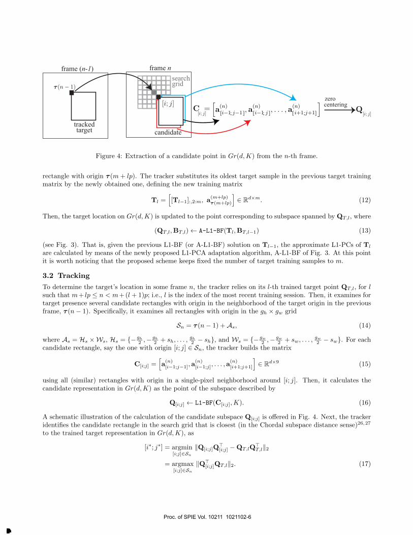
Figure 4: Extraction of a candidate point in Gr(d,K) from the n-th frame.

rectangle with origin τ (m+ lp). The tracker substitutes its oldest target sample in the previous target trainingmatrix by the newly obtained one, defining the new training matrix

Tl =[[Tl−1]:,2:m, a

(m+lp)τ (m+lp)

]∈ Rd×m. (12)

Then, the target location on Gr(d,K) is updated to the point corresponding to subspace spanned by QT,l, where

(QT,l,BT,l)← A-L1-BF(Tl,BT,l−1) (13)

(see Fig. 3). That is, given the previous L1-BF (or A-L1-BF) solution on Tl−1, the approximate L1-PCs of Tl

are calculated by means of the newly proposed L1-PCA adaptation algorithm, A-L1-BF of Fig. 3. At this pointit is worth noticing that the proposed scheme keeps fixed the number of target training samples to m.

3.2 Tracking

To determine the target’s location in some frame n, the tracker relies on its l-th trained target point QT,l, for lsuch that m+ lp ≤ n < m+ (l + 1)p; i.e., l is the index of the most recent training session. Then, it examines fortarget presence several candidate rectangles with origin in the neighborhood of the target origin in the previousframe, τ (n− 1). Specifically, it examines all rectangles with origin in the gh × gw grid

Sn = τ (n− 1) +As, (14)

where As = Hs ×Ws, Hs = {− gh2 ,−

gh2 + sh, . . . ,

gh2 − sh}, and Ws = {− gw

2 ,−gw2 + sw, . . . ,

gw2 − sw}. For each

candidate rectangle, say the one with origin [i; j] ∈ Sn, the tracker builds the matrix

C[i;j] =[a(n)[i−1;j−1],a

(n)[i−1;j], . . . ,a

(n)[i+1;j+1]

]∈ Rd×9 (15)

using all (similar) rectangles with origin in a single-pixel neighborhood around [i; j]. Then, it calculates thecandidate representation in Gr(d,K) as the point of the subspace described by

Q[i;j] ← L1-BF(C[i;j],K). (16)

A schematic illustration of the calculation of the candidate subspace Q[i;j] is offered in Fig. 4. Next, the trackeridentifies the candidate rectangle in the search grid that is closest (in the Chordal subspace distance sense)26,27

to the trained target representation in Gr(d,K), as

[i∗; j∗] = argmin[i;j]∈Sn

‖Q[i;j]Q>[i;j] −QT,lQ

>T,l‖2

= argmax[i;j]∈Sn

‖Q>[i;j]QT,l‖2. (17)

Proc. of SPIE Vol. 10211 1021102-6


0 50 100 150 200 250 300

0

50

100

150

0 100 200 300 400 500 600 700 800

0

20

40

60

80

100

(a) (b)Figure 5: Target-origin error e(n) experienced by the proposed L1-Grassmann tracker (L1-PCA) and the L2-PCA-based alternative, in the video sequences29 (a) “Jogging” and (b) “Face2”.

Finally, the tracker refines this result by searching in the single-pixel neighborhood of [i∗; j∗] (i.e., the rectanglesthat contributed to C[i∗;j∗] in (15)) for the rectangle that is nearest to the trained target point and returns

τ (n) = argmax[i;j]∈[i∗;j∗]+{0,±1}2

‖Q>T,la(n)[i;j]‖2

‖a(n)[i;j]‖2

. (18)

Having concluded the description of both the training and the tracking procedures, in the sequel we provideexperimental studies for the evaluation of the proposed method.

4. EXPERIMENTAL STUDIES

In this section, we evaluate the performance of the proposed method by experimental studies on the video framesequences29 “Jogging” and “Face2”. We compare the performance of the proposed L1-Grassmann tracker withits L2-PCA-based counterpart, for which QT,l ∈ Rd×K contains the K highest-singular-value left-hand singularvectors of the training matrix Tl, calculated by means of standard SVD (instead of L1-BF in (11) and (13)).

To evaluate the tracking performance at frame n, we measure the target-origin error

e(n) = ‖τ (n)− τgt(n)‖2 (19)

where τ(n) is the tracking decision per (18) and τgt(n) is the ground-truth target origin in frame n.

We commence our studies with the “Jogging”29 video stream in which partial and full occlusions, targetdeformation, and out-of-plane rotations are some of the visual tracking challenges that appear. The exactparameters used in this experiment per the notation of Section 3 are: ht = 101, wt = 25, K = 2, p = 9, m = 10,gh = 12, gw = 12, sh = 4, sw = 4. In addition, adaptive histogram equalization was applied.28 In Fig. 5(a) weplot the target-origin error e(n) versus the frame index n for the proposed L1-Grassmann tracker and the L2-PCAbased alternative described above. We mark with blue notches on the bottom of the figure the training frames atwhich the target representation on Gr(d,K) is updated. We observe that both trackers exhibit almost identicalperformance until frame 65 where target occlusion starts. This occlusion lasts for 15 frames during which bothtrackers will have to train 2 times on the occluded target. We observe that L2-PCA gets significantly affectedby the presence of occlusions in the training matrix and, thus, fails to re-locate the target when it re-appears inframe 81. On the other hand, the L1-Grassmann tracker remains sturdy against the occlusion samples among thetraining data, re-locates the target when it re-appears, and continues tracking it accurately until the end of the

Proc. of SPIE Vol. 10211 1021102-7


r

Figure 6: Frames n = 65, 76, 83, and 100 (from left to right) of the “Jogging”29 video stream, with annotatedtracking results for the proposed L1-Grassmann tracker (first row) and the L2-PCA-based alternative (secondrow). Tracking parameters per Section 3 notation: ht = 101, wt = 25, K = 2, p = 9, m = 10, gh = 12, gw = 12,sh = 4, sw = 4.

Figure 7: Frames n = 550, 600, 650, and 700 (from left to right) of the “Face2”29 video stream, with annotatedtracking results for the proposed L1-Grassmann tracker (first row) and the L2-PCA-based alternative (secondrow). Tracking parameters per Section 3 notation: ht = 98, wt = 82, K = 2, p = 8, m = 12, gh = 48, gw = 48,sh = 2, sw = 2.

video stream. In Fig. 6 we present four selected frames of the video, annotated with the tracked rectangles forthe two trackers (L1-Grassmann is presented on the first row of images; the L2-PCA-based tracker is presentedon the second row). Our observations in these frames are in accordance to the numerical results of Fig. 5(a).

Next, we experiment with video sequence “Face2”, which exhibits illumination variations, in-and-out ofplane rotations, and occlusions. In Fig. 5(b), we plot the tracking error for L1-Grassmann and the L2-PCAcounterpart. We observe that L1-Grassmann outperforms the L2-based alternative, exhibiting significantly lowertarget-origin error, especially towards the end of the frame sequence. In Fig. 7 we present four selected framesfrom the video sequence, annotated with the tracked rectangles for the two trackers. The superior performanceof L1-Grassmann is once again clearly illustrated.

Proc. of SPIE Vol. 10211 1021102-8


5. CONCLUSIONS

In this work, we introduced a novel method for robust visual tracking on Grassmann manifolds. The proposedtracker represents the target as a single point on the Grassmann manifold, calculated by means of L1-PCA. Toupdate target representation, the proposed algorithm employs a new, efficient L1-PCA adaptation algorithm.Our experimental studies illustrate that the proposed tracking method leverages the outlier resistance of L1-PCAto achieve robustness against adversities such as target occlusions and illumination variations.

REFERENCES

[1] T. Zhang, S. Liu, N. Ahuja, M.-H. Yang, and B. Ghanem, “Robust visual tracking via consistent low-ranksparse learning,” Int. J. Comp. Vision, vol. 111. pp. 171-190, Jan. 2015.

[2] X. Li, W. Hu, C. Shen, Z. Zhang, A. Dick, and A. V. D. Hengel, “A survey of appearance models in visualobject tracking,” ACM Trans. Intel. Sys. and Tech. (TIST), vol. 4, pp. 1-48, Sep. 2013.

[3] A. W. M. Smeulders, D. M. Chu, R. Cucchiara, S. Calderara, A. Dehghan and M. Shah, “Visual tracking:An experimental survey,” IEEE Trans. Patt. Anal. Mach. Intell., vol. 36, pp. 1442-1468, Nov. 2013.

[4] Y. Wu, J. Lim, and M. H. Yang, “Online object tracking: A benchmark,” in IEEE Proc. Comp. VisionPatt. Recogn. (IEEE CVPR 2013), Portland, OR, Jun. 2013, pp. 2411-2418.

[5] H. Nam and B. Han, “Learning multi-domain convolutional neural networks for visual tracking,” in IEEEProc. Comp. Vision Patt. Recogn. (IEEE CVPR 2016), Las Vegas, NV, Jun. 2016, pp. 4293-4302.

[6] L. Wang, W. Ouyang, X. Wang, and H. Lu, “Visual tracking with fully convolutional networks,” in IEEEProc. Int. Conf. Comp. Vision (IEEE ICCV 2015), Santiago, Chile, Dec. 2015, pp. 3119-3127.

[7] H. Li, L. Yi, and F. Porikli, “DeepTrack: Learning discriminative feature representations by convolutionalneural networks for visual tracking.,” in Proc. British Mach. Vision Conf. (BMVC 2014), Nottingham, UK,Sep. 2014, pp. 1-12.

[8] M. Danelljan, A. Robinson, F. S. Khan, and M. Felsberg, “Beyond correlation filters: Learning continuousconvolution operators for visual tracking,” in Proc. European Conf. Comp. Vision (ECCV 2016), Amster-dam, Netherlands, Oct. 2016, pp. 472-488.

[9] S. Shirazi, M. T. Harandi, B. C. Lovell, and C. Sanderson, “Object tracking via non-Euclidean geometry:A Grassmann approach,” in Proc. Int. Conf. App. Comp. Vision (IEEE WACV 2014), Steamboat Springs,CO, Mar. 2014, pp. 901-908.

[10] D. A. Ross, J. Lim, R.-S. Lin, and M.-H. Yang, “Incremental learning for robust visual tracking,” Int. J.Comput. Vision, vol. 77, pp. 125-141, May 2008.

[11] H. Zhang, S. Hu, L. Luo, X. Ke, “Object tracking using 2DLPP manifold learning,” in Proc. Int. Conf. Inf.Fusion (FUSION 2014), Salamanca, Spain, Jul. 2014, pp. 1-6.

[12] N. Kwak, “Principal component analysis based on L1-norm maximization,” IEEE Trans. Patt. Anal. Mach.Intell., vol. 30, pp. 1672-1680, Sep. 2008.

[13] S. Kundu, P. P. Markopoulos, and D. Pados, “Fast computation of the L1-principal component of real-valued data,” in Proc. IEEE Int. Conf. on Acoust. Speech Signal Process. (IEEE ICASSP 2014), Florence,Italy, May 2014, pp. 8028-8032.

[14] P. P. Markopoulos, S. Kundu, S. Chamadia, and D. A. Pados, “Efficient L1-norm principal-componentanalysis via bit flipping,” IEEE Trans. Signal Process. (submitted).

[15] P. P. Markopoulos, S. Kundu, S. Chamadia, and D. A. Pados, “L1-norm Principal-Component Analysis viaBit Flipping,” in Proc. IEEE Int. Conf. Mach. Learn. App. (IEEE ICMLA 2016), Anaheim, CA, December2016, pp. 326-332.

[16] P. P. Markopoulos, G. N. Karystinos, and D. A. Pados, “Optimal algorithms for L1-subspace signal pro-cessing,” IEEE Trans. Signal Process., vol. 62, pp. 5046-5058, Oct. 2014.

[17] P. Markopoulos, G. Karystinos, and D. Pados, “Some options for L1-subspace signal processing,” in Proc.Int. Symp. Wireless Comm. Systems (ISWCS 2013), Ilmenau, Germany, Aug. 2013, pp. 622-626.

[18] F. Nie, H. Huang, C. Ding, D. Luo, and H. Wang, “Robust principal component analysis with non-greedyl1-norm maximization,” in Proc. Int. Joint Conf. Artif. Intell. (IJCAI), Barcelona, Spain, Jul. 2011, pp.1433-1438.

Proc. of SPIE Vol. 10211 1021102-9


[19] E. J. Candes, X. Li, Y. Ma, and J. Wright, “Robust principal component analysis,” J. ACM, vol. 58, art.11, May 2011.

[20] M. Johnson and A. Savakis, “Fast L1-eigenfaces for robust face recognition,” in Proc. West. New YorkImage Signal Process. Workshop (IEEE WNYISPW 2014), Rochester, NY, Nov. 2014, pp. 1-5.

[21] F. Maritato, Y. Liu, D. A. Pados, and S. Colonnese, “Face recognition with L1-norm subspaces,” in Proc.SPIE Comm. Scient. Sens. Imag., Baltimore, MD, Apr. 2016, pp. 1-8.

[22] P. P. Markopoulos, S. Kundu, and D. A. Pados, “L1-fusion: Robust linear-time image recovery from fewseverely corrupted copies,” in Proc. IEEE Int. Conf. Image Process. (IEEE ICIP 2015), Quebec City,Canada, Sep. 2015, pp. 1225-1229.

[23] Y. Liu and D. A. Pados, “Compressed-sensed-domain L1-PCA video surveillance,” IEEE Trans. Multimedia,vol. 18, pp. 351-363, Mar. 2016.

[24] P. P. Markopoulos, L1-norm Principal-Component Analysis (L1-PCA) code repository [Online]. Available:https://people.rit.edu/pxmeee/soft.html.

[25] M. Pierantozzi, Y. Liu, D. A. Pados, and S. Colonnese, “Video background tracking and foreground extrac-tion via L1-subspace updates,” in Proc. SPIE Commercial + Scientific Sensing and Imaging, Baltimore,MD, Apr. 2016, pp. 985708-1–985708-16.

[26] K. Ye and L.-H. Lim, “Schubert varieties and distances between subspaces of different dimensions,” SIAMJ. Matrix Anal. App., vol. 37, pp. 1176-1197, Sep. 2016.

[27] G. H. Golub and C. F. Van Loan, Matrix Computations, 3rd Ed. Baltimore, MD: The Johns Hopkins Univ.Press, 1996.

[28] K. Zuiderveld, “Contrast limited adaptive histogram equalization,” in Graphics Gems IV. San Diego, CA:Academic Press Professional, 1994. pp. 474-485.

[29] Visual tracker benchmark [Online]. Available: http://cvlab.hanyang.ac.kr/tracker_benchmark.

Proc. of SPIE Vol. 10211 1021102-10


Documents

Visual tracking with L1-Grassmann manifold modeling · Visual Tracking with L1-Grassmann Manifold Modeling Dimitris G. Chachlakis a, Panos P. Markopoulos a, Raj. J. Muchhala b, and