Embed Size (px)
Citation preview

Grassmann Varieties
Ratnadha Kolhatkar
Department of Mathematics and Statistics,
McGill University, Montreal
Quebec, Canada
August, 2004
A thesis submitted to the Faculty of Graduate Studies and Research
in partial fulfillment of the requirements of the degree of
Master of Science
Copyright c© Ratnadha Kolhatkar, 2004


i
Abstract
In this thesis we study the simplest types of generalized Grassmann varieties. The
study involves defining those varieties, understanding their local structures, calculat-
ing their Zeta functions, defining cycles on those varieties and studying their coho-
mology groups.
We begin with the classical Grassmannian G(d, n) and then study a special type
of the Grassmannian, namely the Lagrangian Grassmannian. For a field k and a
subring R ⊂ End(kn) we study the generalized Grassmann variety G(R; d, n) which
is the set of all d-dimensional subspaces of kn that are preserved under R. We study
the local structure of the generalized Grassmann scheme FR := G(R; d, n) and its
zeta function in some particular cases. We study closely the example of a quadratic
field when R is the ring of integers.

ii Abstract

iii
Resume
Dans cette these, nous etudions les plus simples varietes de Grassmann generalisees.
Cette etude consiste a definir ces varietes, a comprendre leur structure locale, a cal-
culer leurs fonctions Zeta, a definir des cycles sur ces varietes et a etudier leurs groupes
de cohomologie.
Nous commencons avec la variete de Grassmann classique G(d, n) et ensuite, nous
etudions specialement la variete de Grassmann Lagrangienne. Pour un corps k donne
et un sous-anneau R ⊂ End(kn), nous etudions la variete de Grassmann generalisee
G(R; d, n), c’est-a-dire l’ensemble de tous les sous-espaces de kn de dimension d qui
sont preserves par R. Nous etudions la structure locale du schema de Grassmann
generalise FR := G(R; d, n) et, dans quelques cas particuliers, sa fonction Zeta. Nous
etudions en detail l’exemple d’un corps quadratique lorsque R est l’anneau des en-
tiers.

iv Resume

v
Acknowledgments
Many people have helped me over past two years and I am thankful to all of them.
First of all, I would like to express my deep gratitude to my supervisors Prof. Eyal
Goren and Prof. Peter Russell for patiently guiding me throughout the course of my
thesis. I am also thankful to them for the kind financial support they provided.
Special thanks to my father for encouraging me to pursue my studies in Canada.
Thanks to my family and my friends for their constant love and moral support.
Je remercie mes amis Quebecois surtout Frederic, Jean-Sebastien, Marc-Hubert
et Eloi qui sont toujours de bons et attentifs amis pour moi. Finalement, je suis
reconnaissante d’avoir ete exposee a ce nouveau monde, a une variete d’experiences
et aux gens d’ici. Mon sejour a Montreal m’a donne de merveilleuses opportunites
d’apprendre et de realiser beaucoup de choses importantes dans la vie.

vi Acknowledgments

vii
Table of Contents
Abstract i
Resume iii
Acknowledgments v
Introduction 1
1 Grassmann Varieties 5
1.1 Grassmann varieties . . . . . . . . . . . . . . . . . . . . . . . . . . . 5
1.1.1 The Grassmannian, basic notions . . . . . . . . . . . . . . . . 5
1.1.2 Review of some exterior algebra . . . . . . . . . . . . . . . . . 6
1.1.3 The Plucker map and coordinates . . . . . . . . . . . . . . . . 7
1.1.4 Examples . . . . . . . . . . . . . . . . . . . . . . . . . . . . . 8
1.1.5 The Grassmannian as an algebraic variety . . . . . . . . . . . 9
1.1.6 An affine covering of the Grassmannian . . . . . . . . . . . . . 15
1.2 The number of points in G(d, n)(Fq) . . . . . . . . . . . . . . . . . . 17
1.2.1 Action of the Galois group on the Grassmannian . . . . . . . . 19
1.2.2 The Zeta function of the Grassmannian . . . . . . . . . . . . 22
1.2.3 The general case G(d, n)⊗ Fq . . . . . . . . . . . . . . . . . . 25
1.2.4 Euler characteristic of the Grassmannian . . . . . . . . . . . . 29

viii TABLE OF CONTENTS
1.3 Schubert calculus . . . . . . . . . . . . . . . . . . . . . . . . . . . . . 29
1.3.1 Schubert conditions and Schubert varieties. . . . . . . . . . . . 30
1.3.2 Some cohomology theory for a topological space and Schubert
cycles . . . . . . . . . . . . . . . . . . . . . . . . . . . . . . . 31
1.3.3 Intersection theory of Schubert cycles . . . . . . . . . . . . . . 37
1.4 The Grassmannian as a scheme . . . . . . . . . . . . . . . . . . . . . 42
1.4.1 Schemes and functors . . . . . . . . . . . . . . . . . . . . . . . 44
1.4.2 Representability of the Grassmann functor . . . . . . . . . . . 47
1.4.3 Computation of the Zeta function of G(d, n) using Schubert
calculus . . . . . . . . . . . . . . . . . . . . . . . . . . . . . . 54
1.4.4 The Zeta function of the Grassmann scheme . . . . . . . . . . 56
2 Lagrangian Grassmannian 59
2.1 Lagrangian Grassmannian . . . . . . . . . . . . . . . . . . . . . . . . 59
2.2 The Lagrangian Grassmannian as an algebraic variety . . . . . . . . . 62
2.2.1 Examples . . . . . . . . . . . . . . . . . . . . . . . . . . . . . 64
2.3 The number of points in L(n, 2n)(Fq) . . . . . . . . . . . . . . . . . . 65
2.3.1 The Zeta function of the Lagrangian Grassmannian . . . . . . 68
2.3.2 Euler characteristic of the Lagrangian Grassmannian . . . . . 69
2.4 Schubert calculus for Lagrangian Grassmannian . . . . . . . . . . . . 70
2.4.1 Cohomology groups of the Lagrangian Grasmannian . . . . . . 71
2.5 Representability of Lagrangian Grassmann functor . . . . . . . . . . . 73
2.5.1 The Zeta function of the Lagrangian Grassmann Scheme . . . 77
3 Other subschemes of the Grassmannian 79
3.1 Representability of the functor fR . . . . . . . . . . . . . . . . . . . . 81
3.2 Properties of FR . . . . . . . . . . . . . . . . . . . . . . . . . . . . . . 83
3.3 Example : Quadratic field . . . . . . . . . . . . . . . . . . . . . . . . 88

TABLE OF CONTENTS ix
3.3.1 The Zeta function : (p) inert in L . . . . . . . . . . . . . . . . 91
3.3.2 The Zeta function : (p) split in L . . . . . . . . . . . . . . . . 95
3.3.3 The Zeta function : (p) ramified in L . . . . . . . . . . . . . . 96
3.4 Zeta function of FR as a scheme over Z . . . . . . . . . . . . . . . . . 98
Conclusion 101

x TABLE OF CONTENTS

1
Introduction
Let us start with the classical Grassmann variety G(d, n), which is the set of all
d-dimensional subspaces of a vector space V of dimension n. The same set can be
considered as the set of all (d−1)-dimensional linear subspaces of the projective space
Pn−1(V ). In that case we denote it by GP(d− 1, n− 1).
In Chapter 1 we see that G(d, n) defines a smooth projective variety of dimension
d(n−d). It is quite interesting to note that the number of Fq-rational points of G(d, n)
equals the standard q-binomial coefficient(
nd
)q
that can be expressed as a polynomial
in powers of q. Consequently, the Zeta function of G(d, n) is easy to calculate and we
see that all odd Betti numbers of the Grassmannian are zero. The Euler characteristic
of G(d, n) comes out to be the usual binomial coefficient(
nd
).
The Schubert calculus is introduced thereafter to understand the cohomology ring
of the Grassmannian, namely H∗(GP(d, n)(C); Z). Schubert calculus helps us solve
many enumerative problems such as : How many lines in 3-space in general intersect
4 given lines? The subject is studied quite intensively in [7, 11, 17, 12, 20]. We mainly
follow [12] to develop the basic notions of the subject and state without proof many
results like the Basis Theorem, Giambelli’s formula and Pieri’s formula. Then we
study the cohomology ring H∗(GP(1, 3)(C); Z) in detail.
In the last few sections of Chapter 1 we see that the construction of the classical
Grassmannian has a natural extension to the category of schemes. Indeed the Grass-
mann scheme GZ(d, n) represents the Grasmann functor g : (rings) → (sets) given
2 Introduction
by
g(T ) = T -submodules K ⊂ T n that are rank d direct summands of T n .
We show the representability of the Grasmann functor following [6]. The Basis Theo-
rem of the Schubert calculus states that the Schubert cycles generate the cohomology
ring H∗(GP(d, n)(C); Z). As one of its applications we compute the Zeta function of
the Grassmannian using the information of cohomology groups in characteristic zero
and get the information of the cohomology groups in characteristic p. Finally, we
compute the Zeta function of the Grassmann scheme GZ(d, n) which comes out to be
a product of Riemann Zeta functions.
In Chapter 2 we discuss a special type of Grassmannian, L(n, 2n), called the La-
grangian Grassmannian; it parametrizes all n-dimensional isotropic subspaces of a
2n-dimensional symplectic space. A lot of symplectic geometry can be found in [14]
and [2]. The Lagrangian Grassmannian L(n, 2n) is a smooth projective variety of di-
mensionn(n+ 1)
2. We then give a similar treatment to the Lagrangian Grassmannian
as to the classical Grassmannian and compute its Zeta function, Euler characteristic
etc.
The Schubert calculus for Lagrangian Grassmannians is discussed for example
in [17, 22]. We mostly follow [22]. Using the Basis Theorem for the Lagrangian
Garssmannian we compute the dimensions of the cohomology groups H i(L(n, 2n); Z).
We then study the representability of the Lagrangian Grassmann functor, which is a
functor l : (rings) → (sets) given by
l(T ) = isotropic T -submodules K ⊂ T 2n that are rank n direct summands of T 2n.
Finally we compute the Zeta function of the Lagrangian Grassmann scheme LZ(n, 2n).
In Chapter 3 we begin with the following set up. Let 0 < d < n be integers,
R ⊆Mn(Z) be a ring, and consider the functor fR : (rings) → (sets) given by
fR(T ) = T -submodules K ⊂ T n that are R-invariant rank d direct summands of T n

3
We show that fR is representable by a scheme FR. We study the local structure of
the scheme FR and its Zeta function in some examples.
We consider in detail the example of a quadratic field L = Q(√D) where D is
a squarefree integer. Let R be the ring of integers in L. Let R1 = R ⊗ Fp. We
concentrate on the case D ≡ 2, 3 (mod 4), study the scheme FR1(Fp) and compute
its Zeta function.

4 Introduction

5
Chapter 1
Grassmann Varieties
In Chapter 1 we discuss in detail the classical Grasssmannian, first as a variety and
then as a scheme. In section 1.1 we discuss the construction of the Grassmannian as
an algebraic variety. We also study an affine cover of the Grassmannian. Section 1.2
discusses the Zeta function of these varieties. In section 1.3 we give an introduction
to the Schubert calculus. This leads us to understand the cohomology ring of the
complex Grassmannian G(d, n)(C) with integer coefficients. In section 1.4 we describe
how the construction of the classical Grassmannian has a natural extension to the
category of schemes. We will also talk on the representability of the Grassmann
functor and the Zeta function of the Grassmann scheme.
1.1 Grassmann varieties
1.1.1 The Grassmannian, basic notions
Recall the construction of a projective space over field k. The projective space Pn(k)
is defined as the collection of all lines in kn+1. Equivalently, it is the set of all
hyperplanes in kn+1. This construction gives rise to a natural question : Why not

6 Grassmann Varieties
consider the set of subspaces in kn+1 of arbitrary dimension? The construction of
Grassmannians has its origin in answering this question. Classically we define the
Grassmannian as follows.
Definition 1.1. Let V be a vector space of dimension n ≥ 2 over field k. Let
0 < d < n be an integer. Then the Grassmannian G(d, n) over k is defined as the set
of all d-dimensional subspaces of V i.e.
G(d, n)(k) = W | W is a k-subspace of V of dimension d.
Alternately, G(d, n) can be considered as the set of all (d− 1)-dimensional linear
subspaces of the projective space Pn−1(k). If we think of the Grassmannian this way,
we denote it by GP(d−1, n−1). The simplest example of the Grassmannian is G(1, n)
which is the set of all 1-dimensional subspaces of the vector space V which is nothing
but the projective space on V .
1.1.2 Review of some exterior algebra
Let R be a commutative ring with unity and let M be an R- module. For each natural
number r let
T r(M) =
R if r = 0,
M ⊗R Tr−1(M) otherwise.
Thus T r(M) = M ⊗R · · · ⊗R M︸ ︷︷ ︸r times
. The tensor product is assosiative and we have a
bilinear map T r(M)×T s(M) → T r+s(M) by which we can define a ring structure on
the direct sum
T (M) :=∞⊕
r=0
T r(M).
In fact, T (M) is an R-algebra. It is called the tensor algebra of M over R. Let
us denote by An(M) the submodule in T n(M) generated by the elements of the type

1.1 Grassmann varieties 7
x1 ⊗ · · · ⊗ xn where xi = xj for some i 6= j. We define
n∧M := T n(M)/An(M).
Also define the exterior algebra of M as the direct sum∧M :=
∞⊕n=0
n∧M.
Let I be the ideal in T (M) generated by x⊗ x | x ∈M. Then we have∧M = T (M)/I.
If w ∈∧r M with, w = u+Ar(M) and w′ ∈
∧sM , with w′ = u′ +As(M), we define
w ∧ w′ = u⊗ u′ +Ar+s(M)
as an element of∧r+sM .
Notation : Let u1, . . . , un ∈ M. The element u1 ⊗ · · · ⊗ un +An(M) is denoted by
u1 ∧ · · · ∧ un.
One has the following Lemma.
Lemma 1.2. [9, Corollary 10.16] Let u1, . . . , un and v1, . . . , vn be two families
of vectors of M related by a matrix A = (aij)n×n of coordinate change, which means,
(v1, . . . , vn) = (u1, . . . , un)(aij)n×n. Then,
v1 ∧ · · · ∧ vn = det(A) · u1 ∧ · · · ∧ un.
1.1.3 The Plucker map and coordinates
We can embed G(d, n) in the projective space P(∧d V ) as follows. Let U be a subspace
of V of dimension d with a basis u1, · · · , ud. Define P (U) as the point of the
projective space P(∧d V ) which is determined by u1 ∧ · · · ∧ ud. The map P ,
P : G(d, n) → P(d∧V ),

8 Grassmann Varieties
is called the Plucker map. By Lemma 1.2, P is a well defined map. Since the wedge
product u1 ∧ · · · ∧ud ∧u = 0 if and only if u ∈ U , it follows that P is injective. Thus,
via P , we may consider G(d, n) as a subset of P(∧d V ). Let e1, . . . , en be a basis
for V . Then the canonical basis for∧d V is given by
ei1 ∧ · · · ∧ eid | 1 ≤ i1 < · · · < id ≤ n.
Let U be a d-dimensional subspace of V with a basis u1, . . . , ud. For 1 ≤ i ≤ d, let
uj =∑n
i=1 aijei. Then the coordinates of P (U) = u1∧· · ·∧ud are called the Plucker
coordinates. These are nothing but the(
nd
)minors of the matrix (aij)1≤i≤n
1≤j≤d.
1.1.4 Examples
Example 1.3. The Grassmannian G(1, n) : Let U be the space spanned by the vector
u1 = a1e1 + · · ·+anen. The Plucker coordinates are the maximal minors of the matrix
(a1, · · · , an). Therefore the Grassmannian G(1, n) ∼= Pn−1 and the Plucker map P
sends U to (a1 : · · · : an).
Example 1.4. The Grassmannian G(2, 4) : Let e1, e2, e3, e4 be a basis for V . The
canonical basis for∧2 V is given by
e1 ∧ e2, e1 ∧ e3, e1 ∧ e4, e2 ∧ e3, e2 ∧ e4, e3 ∧ e4.
Let u1, u2 be a basis for U ∈ G(2, 4) with
u1 = a11e1 + a21e2 + a31e3 + a41e4, u2 = a12e1 + a22e2 + a32e3 + a42e4.
Then,
u1 ∧ u2 = (a11a22 − a12a21)e1 ∧ e2 + (a11a32 − a31a12)e1 ∧ e3
+ (a11a42 − a41a12)e1 ∧ e4 + (a21a32 − a31a22)e2 ∧ e3
+ (a21a42 − a41a22)e2 ∧ e4 + (a31a42 − a41a32)e3 ∧ e4.
So the Plucker coordinates are

1.1 Grassmann varieties 9
(a11a22 − a12a21, a11a32 − a31a12, a11a42 − a41a12, a21a32 − a31a22,
a21a42 − a41a22, a31a42 − a41a32).
We will denote these coordinates by x12, x13, x14, x23, x24, x34 respectively. One ob-
serves that these are indeed the 2× 2 minors of the matrixa11 a12
a21 a22
a31 a32
a41 a42
.
1.1.5 The Grassmannian as an algebraic variety
We observed that G(d, n) can be embedded in the projective space P(∧d V ) via the
Plucker map P . The goal of this section is to show that the image is a closed subset
of PN where N =(
nd
)− 1.
Definition 1.5. Let w ∈∧d V . Let v ∈ V, v 6= 0. We say that v divides w if there
exists u ∈∧d−1 V such that w = v ∧ u.
We have the following Lemma.
Lemma 1.6. Let w ∈∧d V . Let v ∈ V, v 6= 0. Then v divides w if and only if the
wedge product w ∧ v = 0.
Proof. Clearly if v divides w, say w = u ∧ v, then w ∧ v = u ∧ v ∧ v = 0. To see the
other direction let e1, e2, . . . , en be a basis of V with e1 = v. The canonical basis
for∧d V is given by:
ei1 ∧ · · · ∧ eid | 1 ≤ i1 < · · · < id ≤ n.
Let ei1 ∧ · · · ∧ eid = ei1,i2,...,id . Any w ∈∧d V can be written as
w =∑
1≤i1<···<id≤n
ai1,...,idei1,i2,...,id .

10 Grassmann Varieties
Then
v ∧ w =∑
i1<···<id
ai1,...,ide1 ∧ ei1,i2,...,id .
So we see that v ∧ w = 0 if and only if ai1,...,id = 0 for every i1, . . . , id with 1 < i1 i.e.
the vector e1 = v divides w.
Using above lemma we can show that the collection of all vectors v ∈ V dividing
a fixed vector w ∈∧d V is a subspace of V . Indeed, if v1, v2 divide w then
(v1 + v2) ∧ w = v1 ∧ w + v2 ∧ w = 0,
which implies that v1 + v2 divides w. And also v ∧w = 0 implies that av ∧w = 0 for
any scalar a.
Definition 1.7. We say that w ∈∧d V is totally decomposable if there exist
linearly independent vectors v1, . . . , vd ∈ V so that w = v1 ∧ · · · ∧ vd.
Lemma 1.8. Let w ∈∧d V . Then w is totally decomposable if and only if the space
of vectors dividing it is d-dimensional.
Proof. Let w ∈∧d V be a totally decomposable vector. Let w = v1 ∧ · · · ∧ vd for
some linearly independent vi ∈ V . Then by lemma 1.6 the space of vectors dividing w
is given by
U = v ∈ V | v1 ∧ · · · ∧ vd ∧ v = 0.
Thus v ∈ U if and only if it is linearly dependent with the vectors v1, . . . , vd , i.e. U
has a basis v1, . . . , vd. Conversely let U be d-dimensional subspace of V with a
basis v1, . . . , vd. Extend this to a basis v1, . . . , vd, vd+1, . . . , vn for V . Then we
can write w ∈∧d V as
w =∑
1≤i1<···<id≤n
ai1,...,idvi1,i2,...,id .

1.1 Grassmann varieties 11
For all j = 1, . . . , d we have vj ∧ w = 0. Then,
vj ∧ w =∑
1≤i1<···<id≤n
ai1,...,idvj ∧ vi1,i2,...,id
=∑
1≤i1<···<id≤n
ir 6=j
ai1,...,idvj ∧ vi1,i2,...,id .
The right hand side of the above equation is zero if and only if ai1,...,id = 0 unless
some ir = j. Thus,
v1 ∧ w = · · · = vd ∧ w = 0
if and only if ai1,...,id = 0 unless 1, . . . , d ⊂ i1, . . . , id. Then we have
w = ai1,...,idv1 ∧ · · · ∧ vd.
Lemma 1.9. Let w ∈∧d V . Let
ϕw : V →d+1∧
V
be the linear map given by
ϕw(v) = w ∧ v.
Then w is totally decomposable if and only if Ker(ϕw) has dimension d.
Proof. The proof of this lemma follows from the last two lemmas. Note that the
kernel of ϕw is given by Ker(ϕw) = v ∈ V | ϕw(v) = w∧v = 0. This by Lemma 1.6
is the space of vectors dividing w. And by Lamma 1.8, w is totally decomposable if
and only if this space has dimension d.
Theorem 1.10. The image of G(d, n) via the Plucker map P is an algebraic set of
the projective space PN = P(∧d V ).

12 Grassmann Varieties
Proof. We observe that P (G(d, n)) is the set of all totally decomposable vectors w in∧d V . By the Lamma 1.9, it can be identified with the set of vectors w ∈∧d V such
that dim (Ker(ϕw)) = d. Equivalently the rank of the map ϕw is n− d. Now the map∧d V → Hom(V,∧d+1 V ) sending w to ϕw is linear, that is, the entries of the matrix
ϕw ∈ Hom(V,∧d+1 V ) are homogeneous coordinates on P(
∧d V ). Thus the subset
P (G(d, n)) ⊂ P(∧d V ) can be considered as the subvariety defined by the vanishing
of (n− d+ 1)× (n− d+ 1) minors of this matrix.
Unfortunately the equations we get by the above method do not generate the
homogeneous ideal of the Grassmannian. To work out this ideal we have to work a
bit further.
Lemma 1.11. [9, p.18-19] Let V be a vector space over k of dimension n with V ∗ as
the dual space. Let 0 < d < n be an integer. We have a nondegenerate pairing
d∧V ×
n−d∧V →
n∧V ∼= k,
inducing an isomorphism
n−d∧V ∼= (
d∧V )∗ =
d∧V ∗.
Thus, we can identify∧d V naturally (up to scalar multiplication) with the exterior
power∧n−d V ∗ of the dual space.
Now given w ∈ (∧d V ) let w∗ be the corresponding vector in
∧n−d V ∗. This gives
us a linear map
ψw : V ∗ →n−d+1∧
V ∗,
which sends v∗ tow∗ ∧ v∗. By the same argument w ∈∧d V is totally decomposable
if and only if the map ψw has rank d.

1.1 Grassmann varieties 13
Moreover the kernel of ϕw is precisely the annihilator of the kernel of ψw. Take
the transpose maps
ϕtw :
d+1∧V ∗ → V ∗ and ψt
w :n−d+1∧
V → V,
whose images annihilate each other. Thus, a vector w ∈ G(d, n) if and only if for
every pair α ∈∧d+1 V ∗ and β ∈
∧n−d+1 V ,
Ξα,β(w) :=⟨ϕt
w(α) , ψtw(β)
⟩= ϕt
w(α)[ψtw(β)] = 0.
The Ξα,β(w) are quadratic polynomials and they are called the Plucker relations.
It turns out that they do generate the homogeneous ideal of the Grassmannian. This
ideal is called the Plucker ideal.
Example 1.12. The ideal defining the Grassmannian G(2, 4).
As before let e1, e2, e3, e4 be a basis for V . The canonical basis for∧2 V is given
by:
B = e1 ∧ e2, e1 ∧ e3, e1 ∧ e4, e2 ∧ e3, e2 ∧ e4, e3 ∧ e4.
Also the natural basis for∧3 V is given by
B1 = e1 ∧ e2 ∧ e3, e1 ∧ e2 ∧ e4, e1 ∧ e3 ∧ e4, e2 ∧ e3 ∧ e4.
If w =∑aijei ∧ ej, then ϕw : V →
∧3 V sending v to v ∧w is given by the following
matrix a23 −a13 a12 0
a24 −a14 0 a12
a34 0 −a14 a13
0 a34 −a24 a23
.
Thus, the variety G(2, 4) is defined by the ideal I generated by all 3× 3 subdeter-
minants of the above matrix, namely by the entries of the matrix of the adjoint of the
above matrix.

14 Grassmann Varieties
To find the homogeneous ideal defining G(2, 4) one observes that w ∈∧2 V
where V is a vector space over field k, char (k) 6= 2, is totally decomposable if and
only if w ∧w = 0 and in the case when V ∼= k4 we get exactly one quadratic Plucker
relation.
Lemma 1.13. Let k be a field, char (k) 6= 2. Let V be a 4-dimensional vector space
over the field k. Then a vector w ∈∧2 V is totally decomposable if and only if the
corresponding Plucker coordinates satisfy the relation x12x34 − x13x24 + x14x23 = 0.
Proof. Let w ∈∧2 V be totally decomposable. Let w = v1 ∧ v2. Then
w ∧ w = v1 ∧ v2 ∧ v1 ∧ v2 = −v1 ∧ v2 ∧ v2 ∧ v1 = 0.
We can write w as
w = a12e1 ∧ e2 + a13e1 ∧ e3 + a14e1 ∧ e4 + a23e2 ∧ e3 + a24e2 ∧ e4 + a34e3 ∧ e4.
Then by simple computation we get
w ∧ w = 2(a12a34 − a13a24 + a14a23)e1 ∧ e2 ∧ e3 ∧ e4.
Thus w ∧ w = 0 implies that a12a34 − a13a24 + a14a23 = 0. Therefore, if w is totally
decomposable then it satisfies x12x34 − x13x24 + x14x23 = 0. Conversely, let
w = a12e1 ∧ e2 + a13e1 ∧ e3 + a14e1 ∧ e4 + a23e2 ∧ e3 + a24e2 ∧ e4 + a34e3 ∧ e4
be a vector satisfying
a12a34 − a13a24 + a14a23 = 0. (1.1)
Then w ∧ w = 0. Now we want to show that w is totally decomposable. For this we
consider the following different cases.
1. Suppose first that a12 6= 0, a13 6= 0. Then using equation 1.1 we can show that
w =
(a12e1 +
a23a12
a13
e2 +a23a14 − a13a24
a13
e4
)∧(e2 +
a13
a12
e3 +a14
a12
e4
).

1.1 Grassmann varieties 15
2. Let a12 = 0 = a13. Then equation 1.1 yields a14a23 = 0. So we have a14 = 0 or
a23 = 0 or both are zero. If in this case a14 = 0 = a23 we can write w as
w = a24e2 ∧ e4 + a34e3 ∧ e4 = (a24e2 + a34e3) ∧ e4.
If a14 = 0, a23 6= 0 then we can decompose w as
w = (a23e2 − a34e4) ∧(e3 +
a24
a23
e4
).
If a14 6= 0, a23 = 0, w can be written as
w = (a14e1 + a24e2 + a34e3) ∧ e4.
So w is totally decomposable.
3. If a12 = 0, a13 6= 0, equation 1.1 gives us that a13a24 = a14a23 and w can be
decomposed as
w = (a13e1 + a23e2 − a34e4) ∧(e3 +
a14
a13
e4
).
4. If a13 = 0, a12 6= 0, equation 1.1 gives us that a12a34 = −a14a23 and w in this
case can be decomposed as
w = (a12e1 − a23e3 − a24e4) ∧(e2 +
a14
a12
e4
).
Thus we see that in all the cases w is totally decomposable.
1.1.6 An affine covering of the Grassmannian
Abstractly the Grassmannian G(d, n) can be considered as a union of open sets each
isomorphic to the affine space Ad(n−d). To see this, let Γ ⊂ V be a fixed subspace of V
of dimension n−d. Let ei1 , . . . , ein−d be a basis for Γ. Let λ = P (Γ) = ei1∧· · ·∧ein−d
be the image of Γ via the Plucker map P . We can view λ as a linear form on
16 Grassmann Varieties
P(∧d V ) as follows. For v ∈
∧d V define λ(v) := v ∧ λ ∈∧n V ∼= k. We can check
that whether λ(v) is zero or not is well defined and writing everything in terms of
coordinates we get that λ is a homogeneous polynomial of degree 1. We then get the
affine variety
UΓ = [P(d∧V )− Z(λ)] ∩G(d, n)
= P (K) |K ∈ G(d, n), P (K) ∧ λ 6= 0 .
Now P (K) ∧ λ 6= 0 means that K is spanned by d elements none of which is linearly
dependent with ei1 , . . . , ein−d. So we can find a basis of V with first d elements span-
ning K and the remaining elements spanning Γ. Therefore V = K⊕
Γ. Conversely
suppose that V = K⊕
Γ. Then we have such a basis for K as these basis vectors
together with ei1 , . . . , ein−dare linearly independent. So, P (K) ∧ λ 6= 0.
Proposition 1.14. Let Γ ⊂ V be a fixed subspace of dimension n − d. Fix a sub-
space K0 of V such that V = Γ ⊕ K0. Then in the above notations, UΓ is given
by
UΓ∼= Hom (K0,Γ) ∼= kd(n−d).
Proof. For ϕ ∈ Hom(K0,Γ) we associate to it its graph (t, ϕ(t)) | t ∈ K0 which is
a d-dimensional subspace of V . Also given K ∈ G(d, n) such that K ⊕Γ = V we can
see that K arises as a graph of some ϕ ∈ Hom(K0,Γ). If w ∈ K0 there exists unique
u ∈ Γ such that (w, u) ∈ K. Then we define ϕ(w) = u. Thus we can identify the
set UΓ with Hom (K0,Γ). Moreover, the identification UΓ∼= Hom (K0,Γ) ∼= kd(n−d)
respects the Zariski topology, i.e.,
UΓ∼= Hom (K0,Γ) ∼= Ad(n−d).
We now see this condition in terms of coordinates. Let e1, e2, . . . , en be a basis
for V ∼= kn and let Γ be spanned by ed+1, . . . , en. Then if K ∈ UΓ and if K has basis

1.2 The number of points in G(d, n)(Fq) 17
v1, . . . , vd with vj =∑n
i=1 aijej, then the first d × d minors of the matrix (aij) are
nonzero. As P (K) does not depend on the choice of the basis, the basis v1, . . . , vd
may be chosen so that the matrix (aij) has the form
(aij) =
1
1. . .
1
b1,1 . . . b1,d
......
...
bn−d,1 . . . bn−d,d
.
Thus, any K ∈ UΓ can be represented as the column space of the unique matrix of the
above form, the entries bi,j of this matrix give the bijection between UΓ and kd(n−d).
Corollary 1.15. The dimension of the Grassmannian G(d, n) is d(n− d).
Proof. Since the Grassmannian G(d, n) can be covered by open sets isomorphic to
the affine space Ad(n−d), an immediate consequence is that
dim(G(d, n)) = d(n− d).
1.2 The number of points in G(d, n)(Fq)
Let k be a perfect field. The Galois Group Γ = Gal(k/k) acts on the projective space
Pn(k) as follows. For σ ∈ Γ and (a0 : a1 : · · · : an) ∈ Pn(k), we define
σ(a0 : · · · : an) = (σ(a0) : · · · : σ(an)).

18 Grassmann Varieties
The action is well defined since ∀λ ∈ k∗ we have
σ(λa0 : · · · : λan) = (σ(λa0) : · · · : σ(λan))
= (σ(λ)σ(a0) : · · · : σ(λ)σ(an))
= σ(a0 : · · · : an).
One can easily verify that
1. Id(a0 : · · · : an) = (a0 : · · · : an),
2. σ1σ2(a0 : · · · : an) = σ1(σ2(a0 : · · · : an)).
Lemma 1.16. The Galois group Γ = Gal(k/k) acts on Pn(k) and the fixed points are
precisely the points in Pn(k) i.e.
u = (a0 : · · · : an) ∈ Pn(k) | σ(u) = u, ∀ σ ∈ Γ = Pn(k).
Proof. Suppose that for σ ∈ Γ,
σ(a0 : · · · : an) = (a0 : · · · : an).
Then for every σ there is a λσ such that
σ(ai) = λσai, i = 0, · · · , n.
Without loss of generality let a0 6= 0. Then for σ ∈ Γ we have
σ(ai) =σ(a0) · ai
a0
for i = 0, 1, · · · , n.
Therefore, we haveai
a0
= σ
(ai
a0
),∀σ ∈ Γ,
that is,ai
a0
∈ k ∀i = 0, · · · , n.

1.2 The number of points in G(d, n)(Fq) 19
So we get
(a0 : a1 : · · · : an) = (1 : a1/a0 : · · · : an/a0) ∈ Pn(k).
Thus, the Galois group Γ = Gal(k/k) acts on Pn(k) and the fixed points are
precisely the points in Pn(k).
On similar lines we will now consider the action of the Galois group on the Grass-
mannian G(d, n) and use that to calculate the number of points of G(d, n)(Fq).
1.2.1 Action of the Galois group on the Grassmannian
Without loss of generality suppose that the n-dimensional vector space V is (k)n.
Then G(d, n) is the collection of all d-dimensional subspaces of (k)n and Γ = Gal(k/k)
acts on it as follows. For U ∈ G(d, n) and σ ∈ Γ define
σ(U) = σ(x1, x2, . . . , xn) | (x1, . . . , xn) ∈ U,
where,
σ(x1, x2, . . . , xn) = (σ(x1), . . . , σ(xn)).
It is easy to verify that if U has a basis v1, v2, . . . , vd then σ(U) is again a d-
dimensional subspace of (k)n with a basis σ(v1), . . . , σ(vd). We therefore get an
action of Γ on G(d, n)(k). We can also think of G(d, n) as embedded in the projective
space PN = P(∧d V ) via the Plucker map P : G(d, n) → PN and we may consider the
action of Γ on it as induced by the action on the projective space. Note that the two
actions of Γ on G(d, n) are compatible, this means, for σ ∈ Γ, U ∈ G(d, n), we have,
σ(P (U)) = P (σ(U)).
Definition 1.17. We say that U ∈ G(d, n) is Γ-invariant if σ(U) = U for all σ ∈ Γ.
Lemma 1.18. A subspace U ∈ G(d, n)(k) is Γ-invariant if and only if U has a
basis w1, w2, . . . , wd with each wi ∈ kn.

20 Grassmann Varieties
Proof. Clearly if the subspace U has a basis w1, w2, . . . , wd with each wi ∈ kn
then U is Γ-invariant. Now let U be a d- dimensional subspace of V spanned by the
vectors v1, v2, · · · , vd such that σ(U) = U, ∀ σ ∈ Γ. We prove that there is a basis
w1, w2, . . . , wd of U such that
∀σ ∈ Γ , σ(wi) = wi, i = 1, 2, · · · , d.
As σ(U) = U, ∃A(σ) ∈ GL(d, k) such that
σ
( v1v2
...vd
)= A(σ)
( v1v2
...vd
).
Then we have,
A(στ)
( v1v2
...vd
)= σ
[τ
( v1v2
...vd
)]= σ
[A(τ)
( v1v2
...vd
)]
= σ[A(τ)]σ
( v1v2
...vd
)= σ[A(τ)]A(σ)
( v1v2
...vd
).
So we have A(σ τ) = [σA(τ)]A(σ), i.e., A(σ) is a 1-cocycle and using the result that
H1(Γ, GL(n, k)) is the identity [18, p.159] we get that the 1-cocycle A(σ) splits.
Therefore, there exists B ∈ GL(d, k) such that B = (σB)A(σ). Now let( w1w2
...wd
)= B
( v1v2
...vd
).
Then we have( w1w2
...wd
)= B
( v1v2
...vd
)= (σB) ·A(σ)
( v1v2
...vd
)= (σB) ·σ
( v1v2
...vd
)= σ
[B
( v1v2
...vd
)]= σ
( w1w2
...wd
).
So for all σ ∈ Γ , σ(wi) = wi , i = 1, 2, · · · d, which implies that U has a basis
w1, w2, · · · , wd with wi ∈ kn ( as (k)Γ = k).
We now use these results to calculate the cardinality of G(d, n)(Fq).

1.2 The number of points in G(d, n)(Fq) 21
Proposition 1.19. The number of points of G(d, n)(Fq) is given by
|G(d, n)(Fq)| =f(n)
f(d) · f(n− d) · qd(n−d).
where f(n) = (qn − 1)(qn − q) · · · (qn − qn−1).
Proof. Let k = Fq. Then we have | G(d, n)(k) | = | [G(d, n)(k)]Γ | which is the
number of d-dimensional subspaces of (k)n that are Γ- invariant. Let J denote the
collection of all ordered bases v1, v2, . . . , vd with each vi ∈ kn. Then J defines
an open subset of (kn)d. By Lemma 1.18 it follows that to compute the number of
subspaces which are Γ-invariant one can compute the number of elements of J and
take into account how many different ordered bases give rise to the same element of
G(d, n). Let U ∈ G(d, n). The cardinality of G(d, n)(Fq) is given by
number of points of J
number of ordered bases for each U.
The number of ordered bases for each U is |GL(d, k)|. So we get
|G(d, n)(Fq)| =|J |
|GL(d, k)|.
Now we find |J |. The general linear group GL(n, k) = Aut(kn) acts naturally on J
and the action is transitive. The stabilizer of X = e1, . . . , ed has the block matrix
of the form Id ∗
0 GL(n− d, k)
.
Hence,
|J | = |GL(n, k)||stabilizer(X)|
=1
qd(n−d)· |GL(n, k)||GL(n− d, k)|
.
Then we have
|G(d, n)(Fq)| =|GL(n,Fq)|
|GL(d,Fq)| · |GL(n− d,Fq)| · qd(n−d)=
f(n)
f(d) · f(n− d) · qd(n−d),
where f(n) = (qn − 1)(qn − q) · · · (qn − qn−1).
22 Grassmann Varieties
1.2.2 The Zeta function of the Grassmannian
Let X be a smooth projective variety over k = Fq. The Zeta function of X is defined
by
Z(X, t) := exp
(∞∑
r=1
Nr.tr
r
)∈ Q[[t]],
where Nr is the number of points of X defined over Fqr . Let X be a non-singular
projective variety of dimension n. Then the Weil conjectures [8, Appendix C], proven
by Deligne and Dwork, concerning Z(X, t) are:
1. Rationality : Z(X, t) is a rational function in t.
2. Functional equation : Z(X, t) satisfies the functional equation namely,
Z
(X,
1
qnt
)= ±q
nE2 tEZ(X, t),
where E is the Euler characteristic of X which can be defined as the self inter-
section number of the diagonal 4 ⊂ X ×X.
3. Riemann hypothesis : We can write
Z(X, t) =P1(t) · P3(t) · · ·P2n−1(t)
P0(t) · P2(t) · · ·P2n(t),
where P0(t) = 1 − t, P2n(t) = 1 − qnt and for each 1 ≤ i ≤ 2n − 1, Pi(t) is a
polynomial with integer coefficients which can be written as
Pi(t) =
bi∏j=1
(1− ωijt),
where ωij are algebraic integers with |ωij| = qi/2. Given Z(X, t), these condi-
tions uniquely determine the polynomials Pi(t).
4. Cohomological interpretation: Define the i-th Betti number bi of X as
the degree of the polynomial Pi(t) where Pi(t) is as in 3. Then we have the

1.2 The number of points in G(d, n)(Fq) 23
Euler characteristic, E =∑
(−1)ibi. Suppose now that X is obtained from a
variety Y defined over an algebraic number ring R, by reduction modulo a prime
ideal p of R. Then bi is equal to the i-th Betti number of the topological space
Yh = Y ⊗R C, i.e., bi is the rank of the singular cohomology group H i(Yh; Z).
As seen before, the Grassmannian G(d, n) can be embedded into the projective
space P(∧d V ) via the Plucker map. Recall that G(d, n) can be covered by open affine
spaces of dimension d(n−d), so it is a smooth projective variety of dimension d(n−d)
which may be considered over any finite field Fq. We now calculate the Zeta function
of some Grassmannians over Fq. We will also see the rationality of the Zeta function
and the functional equation in a few examples.
Example 1.20. Projective space G(1, n+ 1) = Pn. One has
|Pn(Fq)| = 1 + q + q2 + · · ·+ qn,
and so,
Nr = |Pn(Fqr)| = 1 + qr + q2r + · · ·+ qnr,
Z(t) := Z(PnZ ⊗ Fq, t) = exp
(∞∑
r=1
(1 + qr + · · ·+ qnr)tr
r
).
Taking logarithm on both sides and using the formula : ln(1−t) = −t−t2/2−t3/3−. . . ,
we get,
ln[Z(t)] =∞∑
r=1
(1 + qr + ....+ qnr)tr
r
= − ln(1− t)− ln(1− qt)− · · · − ln(1− qnt).
= − ln[(1− t) · · · (1− qnt)].
It follows that
Z(PnZ ⊗ Fq, t) =
1
(1− t)(1− qt) · · · (1− qnt).

24 Grassmann Varieties
We see that Pi(t) = 1 for all odd i and P2i(t) = 1 − qit for i = 0, 1, 2, · · · , n. The
degree of Pi(t) is zero for i odd and 1 for i even; odd Betti numbers are zero and the
even Betti numbers are equal to 1. The Euler characteristic is E =∑bi = n+1. We
now verify the functional equation
Z
(Pn
Z ⊗ Fq,1
qnt
)=
1
(1− 1/qnt)(1− q/qnt) · · · (1− qn/qnt)
=qnt · qn−1t · · · qt · t
(1− t)(1− qt) · · · (1− qnt)
= qn(n+1)/2 · tn+1
= qn·E/2 · tE · Z(Pn ⊗ Fq, t).
Thus, the functional equation is verified. Also note that the numbers b0, b1, · · · bnmatch with the Betti numbers of the complex projective space Pn(C) and the number
E = n+ 1 matches with the Euler characteristic of Pn(C).
Example 1.21. The Grassmannian G(2, 4)⊗Fq. By the general formula, the dimen-
sion of G(2, 4) is 4. We first calculate Nr. By Proposition 1.19,
|G(2, 4)(Fq)| =(q4 − 1)(q4 − q)(q4 − q2)(q4 − q3)
(q2 − 1)2(q2 − q)2q4
= (q2 + 1)(q2 + q + 1) = 1 + q + 2q2 + q3 + q4,
and so
Nr = 1 + qr + 2q2r + q3r + q4r.
It follows that
Z(G(2, 4)⊗ Fq, t) = exp
(∞∑
r=1
(1 + qr + 2q2r + q3r + q4r)tr
r
)=
1
(1− t)(1− qt)(1− q2t)2(1− q3t)(1− q4t).
We see that Z(t) is a rational function in t. The polynomial Pi(t) = 1 for all odd i. We
have, P0(t) = 1−t, P2(t) = 1−qt, P4(t) = (1−q2t)2, P6(t) = 1−q3t, P8(t) = 1−q4t.

1.2 The number of points in G(d, n)(Fq) 25
The Betti numbers bi are zero for all odd i and b0 = 1, b2 = 1, b4 = 2, b6 = 1, b8 = 1.
The Euler characteristic E =∑bi = 6. We now verify the functional equation for
X = G(2, 4)⊗ Fq
Z
(X,
1
q4t
)=
1
(1− 1/q4t)(1− q/q4t)(1− q2/q4t)2(1− q3/q4t)(1− q4/q4t)
= q4t · q3t · (q2t)2 · qt · t · Z(X, t)
= q12 · t6 · Z(X, t)
= qnE/2tE · Z(X, t),
and the functional equation is verified.
Example 1.22. The Grassmannian G(2, 5)⊗ Fq. We have
|G(2, 5)(Fq)| =(q5 − 1)(q5 − q)(q5 − q2)(q5 − q3)(q5 − q4)
(q2 − 1)(q2 − q)(q3 − 1)(q3 − q)(q3 − q2)q6
= 1 + q + 2q2 + 2q3 + 2q4 + q5 + q6,
and so,
Nr = 1 + qr + 2q2r + 2q3r + 2q4r + q5r + q6r.
It follows that
Z(G(2, 5)⊗ Fq, t) = exp
(∞∑
r=1
(1 + qr + 2q2r + 2q3r + 2q4r + q5r + q6r)tr
r
),
and by similar calculations we get
Z(G(2, 5)⊗ Fq, t) =1
(1− t)(1− qt)(1− q2t)2(1− q3t)2(1− q4t)2(1− q5t)(1− q6t).
1.2.3 The general case G(d, n)⊗ Fq
By proposition 1.19 we get
Nr = |G(d, n)(Fqr)|
=(qnr − 1)(qnr − qr) · · · (qnr − q(n−1)r)
(qdr − 1) · · · (qdr − q(d−1)r) · (q(n−d)r − 1) · · · (q(n−d)r − q(n−d−1)r) · qrd(n−d).

26 Grassmann Varieties
For simplicity set qr = l. So we have
Nr =(ln − 1)(ln − l) · · · (ln − ln−1)
(ld − 1) · · · (ld − ld−1) · (ln−d − 1) · · · (ln−d − ln−d−1) · ld(n−d)
Multiplying and dividing by ld(n−d) and simplifying we get
Nr =(ln − 1)(ln−1 − 1) · · · (ln−d+1 − 1)
(ld − 1)(ld−1 − 1) · · · (l − 1).
This is the usual Gaussian binomial coefficient or l-binomial coefficient(
nd
)l
and it can be interpreted as a polynomial in l. To be more precise(n
d
)l
=
d(n−d)∑i=0
bili.
where the coefficient bi of li is the number of distinct partitions of i elements that
fit inside a rectangle of size d × (n− d). For a detailed discussion on the Gaussian
binomial coefficient refer to [1, section 13.5]. We illustrate this with examples.
Example 1.23. Find the Gaussian binomial coefficient(42
)l.
Suppose(42
)l= b0 + b1l + b2l
2 + b3l3 + b4l
4. We summarize the number of partitions
of i for i = 0, 1, 2, 3, 4 in the following table.
i admissible partitions of i bi = number of admissible partitions
0 1
1 1 1
2 2, 1, 1 2
3 2, 1 1
4 2, 2 1
Hence we get (4
2
)l
= 1 + l + 2l2 + l3 + l4,
i.e., Nr = 1+qr+2q2r+q3r+q4r. Note that this calculation matches with the calculation
done before while calculating the Zeta function of G(2, 4)⊗ Fq.

1.2 The number of points in G(d, n)(Fq) 27
Example 1.24. Find the Gaussian binomial coefficient(52
)l.
Suppose(52
)l= b0 + b1l+ b2l
2 + b3l3 + b4l
4 + b5l5. We summarize the number of allowed
partitions of i for i = 0, 1, 2, 3, 4, 5, 6 in the following table
i admissible partitions of i bi = number of admissible partitions
0 1
1 1 1
2 2, 1, 1 2
3 2, 1, 1, 1, 1 2
4 2, 2, 2, 1, 1 2
5 2, 2, 1 1
6 2, 2, 2 1
Hence we have
(5
2
)l
= 1 + l + 2l2 + 2l3 + 2l4 + l5 + l6,
i.e., Nr = 1 + qr + 2q2r + 2q3r + 2q4r + q5r + q6r. Again this calculation matches with
the calculation done before while calculating the Zeta function of G(2, 5)⊗ Fq.
Example 1.25. Find the Gaussian binomial coefficient(63
)l.
Suppose
(6
3
)l
= b0 + b1l + b2l2 + b3l
3 + b4l4 + b5l
5 + b6l6 + b7l
7 + b8l8 + b9l
9.
We summarize the number of allowed partitions of i for i = 0, 1, . . . , 9 in the following
table

28 Grassmann Varieties
i admissible partitions of i bi = number of admissible partitions
0 1
1 1 1
2 2, 1, 1 2
3 3, 2, 1, 1, 1, 1 3
4 3, 1, 2, 2, 2, 1, 1 3
5 2, 2, 1, 3, 2, 3, 1, 1 3
6 2, 2, 2, 3, 2, 1, 3, 3 3
7 3, 2, 2, 3, 3, 1 2
8 3, 3, 2 1
9 3, 3, 3 1
Hence we get(6
3
)l
= 1 + l + 2l2 + 3l3 + 3l4 + 3l5 + 3l6 + 2l7 + l8 + l9,
i.e., Nr = 1 + qr + 2q2r + 3q3r + 3q4r + 3q5r + 3q6r + 2q7r + q8r + q9r.
Now we consider the general case. Regarding l as a formal variable, it is possible
to express the coefficient Nr of any Grassmannian G(d, n)⊗ Fq as
Nr =
d(n−d)∑i=0
bili.
where bi = bi(d, n, l) can be found as explained before and the Zeta function of the
Grassmannian then comes out to be
Z(G(d, n)⊗ Fq, t) =1
(1− t)b0(1− qt)b1 · · · (1− qd(n−d)t)bd(n−d).
From this we observe that all the odd Betti numbers of the Grassmannians are zero.
As we shall see in section 1.4.3, the numbers bi here are the even topological Betti num-
bers of the complex Grassmannian X(C) = G(d, n)(C) , i.e., bi = dim H2i(X(C),Z).
The odd Betti numbers of X(C) are zero.

1.3 Schubert calculus 29
1.2.4 Euler characteristic of the Grassmannian
Consider the Grassmannian G(d, n). As seen in the last section, the odd Betti num-
bers of the Grassmannian are zero and the even Betti numbers are related to the
Gaussian binomial coefficient by (n
d
)l
=
d(n−d)∑i=0
bili.
Putting l = 1 in the above expression we immediately get the Euler characteristic of
the Grassmannian as
E =
d(n−d)∑i=0
bi =
(n
d
)1
.
Referring to [1] section 13.5, Theorem 1, the Gaussian binomial coefficient(
nd
)1
is the
usual binomial coefficient(
nd
). Hence the Euler characteristic of G(d, n) is
(nd
).
1.3 Schubert calculus
Let GP(d, n) be the set of all d-dimensional subspaces (or d-planes) of the n dimen-
sional complex projective space Pn i.e. in our old notation, GP(d, n) = G(d+1, n+1).
Now onwards we always refer to the projective space Pn over the complex numbers C.
Let N =(
n+1d+1
)− 1. As seen before there is a natural way of associating a point of PN
to a d-plane L ∈ GP(d, n) and the coordinates of L regarded as elements of PN are
called the Plucker coordinates. This embedding of GP(d, n) into PN makes it into a
manifold of dimension (d+ 1)(n− d). The Schubert Calculus describes the cohomol-
ogy ring of GP(d, n) say with integer coefficients when the base field is C. The subject
started with a typical enumerative problem: How many lines in 3-space in general,
intersect 4 given lines? The answer to this question lies in finding the degree of some
Schubert cycles. The fundamental theorem of Schubert calculus also helps under-
stand the generalization of Bezout’s theorem. We now develop important notions of
the subject.

30 Grassmann Varieties
1.3.1 Schubert conditions and Schubert varieties.
We are interested in finding a necessary and sufficient condition for a d-plane in the
projective space Pn to intersect a given sequence of linear spaces of Pn in a prescribed
way. Let A : A0 ⊂ A1 ⊂ · · · ⊂ Ad be a strictly increasing sequence of d + 1 linear
spaces of Pn. Such a sequence is called a flag. Let dimAi = ai for each i. If we take Ai
to be consisting of all points in Pn of the form (x0 : x1 : · · · : xi : 0 : 0 : 0 : · · · : 0) then
we call A the standard flag.
Definition 1.26. A d-plane L in Pn is said to satisfy the Schubert condition
defined by the flag A if dim(Ai
⋂L) ≥ i for all i = 0, 1, · · · , d.
Thus a d-plane satisfying the Schubert conditions with respect to the flag A in-
tersects A0 at least in a point, A1 at least in a line etc., and it lies in Ad. It can be
seen that the condition dim(Ai
⋂L) ≥ i for i = 0, · · · , d is satisfied if and only if the
Plucker coordinates of the d-plane L satisfy certain linear relations in addition to the
quadratic relations. Indeed the collection of all such planes defines a variety. For the
proof of this refer to [12, p.1066-1070].
Definition 1.27. The collection of all d-planes in GP(d, n) satisfying the Schubert
condition with respect to a given flag A defines a projective variety. It is known as
the Schubert variety Ω(A) corresponding to the flag A.
In fact this variety is the intersection of a linear subspace of Pn with GP(d, n).
The dimension of the Schubert variety Ω(A) with A as above is∑d
i=0(ai− i). For the
proof of this fact refer to [12, p.1071].
Example 1.28. Let A0 be a line in P3. Let A1 = P3. Let A : A0 ⊂ A1 = P3 be a
flag in P3. Then Ω(A) is the set of all lines L in P3 such that dim(L ∩ A0) ≥ 0 and
dim(L ∩ P3) ≥ 1. As L ∩ P3 = L, the second condition is automatically satisfied and
Ω(A) is the set of all lines L in P3 that intersect the line A0.

1.3 Schubert calculus 31
Example 1.29. Suppose that dim(Ai) = i ∀i = 0, 1, · · · , d. Then Ω(A) consists of
the single d-plane Ad.
Example 1.30. Suppose that dim(Ai) = i ∀i = 0, 1, · · · , d−1. Let dim(Ad) = d+r.
Then Ω(A) consists of all d-dimensional subspaces of GP(d, n) which contain Ad−1 and
which are contained in Ad and such a set is isomorphic to Pr.
Example 1.31. Suppose that dim(Ai) = n−d+i ∀i = 0, 1, · · · , d. Then, the Schubert
variety Ω(A) is GP(d, n).
1.3.2 Some cohomology theory for a topological space and
Schubert cycles
We recall some singular homology theory. For the details of the subject one can refer
to [10, Chapters 2 and 3]. An n-simplex is the smallest convex set in Rm containing
n + 1 points v0, v1, . . . , vn that do not lie in a hyperplane of dimension less than n.
The points vi are the vertices of the simplex, and the simplex itself will be denoted
by [v0, · · · , vn]. The standard n simplex is given by
∆n = (t0, . . . , tn) ∈ Rn+1 |∑
i
ti = 1, ti ≥ 0 ∀ i.
A singular n-simplex in a topological space X is a continuous map σ : ∆n → X.
Let Cn(X) be the free abelian group with basis consisting of the set of all singu-
lar n-simplices in X. Elements of Cn(X) are called singular n-chains. These are
formal sums∑
i ni σi, ni ∈ Z, almost all zero and σi : ∆n → X. The boundary
of the n-simplex [v0, · · · , vn] consists of the various (n − 1)-dimensional simplices
[v0, . . . , vi, . . . , vn], where the symbol hat over vi indicates that this vertex is deleted
from the sequence v0, · · · , vn. The boundary map ∂n : Cn(X) → Cn−1(X) is defined
by
∂n(σ) =∑
i
(−1)i σ| [v0, . . . , vi, . . . , vn].

32 Grassmann Varieties
We have ∂n · ∂n+1 = 0 and we define the n-th homology group of X by
Hn(X) = Ker ∂n/Im ∂n+1.
We now define the cohomology of a space.
Definition 1.32. Let X be a topological space and G be an abelian group. We
define the group Cn(X;G) of singular n-cochains with coefficients in G to be the dual
group Hom(Cn(X);G) of the singular chain group Cn(X). The coboundary map
δn : Cn(X;G) → Cn+1(X;G) is the dual of the map between n chains and we have
δn · δn−1 = 0. Elements of Ker δn are called n-cocycles and the elements of Im δn are
called n-coboundaries. We define the cohomology group Hn(X;G) as the quotient
Ker δn/Im δn−1.
Definition 1.33. Cup product: We consider the cohomology with coefficients in a
ring R (e.g. in Z). For cochains φ ∈ Ck(X;R), ψ ∈ C l(X,R), the cup product
φ ∪ ψ ∈ Ck+l(X;R) is the cochain whose value on a singular simplex σ : ∆k+l → X
is given by
(φ ∪ ψ)(σ) = φ(σ|[v0, . . . , vk]) ψ(σ|[vk . . . vk+l]).
The cup product of cochains is bilinear and associative. It can be shown that the cup
product of cochains induces a cup product of cohomology classes namely
Hk(X;R)×H l(X;R) → Hk+l(X;R).
This product is bilinear, associative and distributive since at the level of cochains the
product has these properties. If R has an identity element, there is an identity element
for the cup product. Note that the cup product is, in general, not commutative.
Instead it is anti-commutative. If φ ∈ Ck(X;R), ψ ∈ C l(X,R) then one has (in
cohomology)
φ ∪ ψ = (−1)klψ ∪ φ.

1.3 Schubert calculus 33
Definition 1.34. Cap product: LetX be a topological space. Let R be the coefficient
ring. For for σ : ∆k → X and φ ∈ C l(X;R), k ≥ l, define an R-bilinear cap product
∩ : Ck(X;R)× C l(X;R) → Ck−l(X;R) by
σ ∩ φ = φ(σ|[v0, . . . , vl])σ|[vl, . . . , vk].
This induces a cap product in homology and cohomology namely
Hk(X;R)×H l(X;R) → Hk−l(X;R),
which is R-linear in each variable.
Definition 1.35. The cohomology ring: Define the cohomology ring H∗(X;R) as
the graded ring H∗(X;R) :=⊕
n≥0Hn(X;R). Elements of H∗(X;R) are finite sums∑
i αi with αi ∈ H i(X;R). We define the product (∑
i αi).(∑
i βi) =∑
i,j αi ∪ βj.
This makes H∗(X,R) into a ring with identity if R has identity.
Poincare Duality: The Poincare duality relates the homology and the cohomology
groups of a compact oriented triangulated n-manifold X in dimension k and n − k.
The cohomology groups form a graded ring with respect to cup product and the
homology groups form a module over the cohomology ring by means of cap product.
The canonical map H i(X;R) → Hn−i(X;R) taking α to α ∩ [X] is an isomorphism.
This map is called the Poincare duality map. When X is a non-singular complex
projective variety of dimension n, it is an oriented real 2n-manifold and the group
H2n(X;R) has a canonical generator [X]. A closed subvariety V of dimension k of a
projective variety X determines a class [V ] in H2k(X;R) and, by Poincare duality, we
have the class in H2c(X;R) = H2k(X;R), where c is codimension of V in X. Thus, if
X is smooth proper over C and V is a subvariety of codimension k then, there exists
associated to V a cohomology class η(Y ) ∈ H2k(X; Z). This map extends by linearity
to cycles.

34 Grassmann Varieties
Applying this to Schubert varieties we see that Ω(A) defines a cohomology class in
the cohomology ringH∗(GP(d, n); Z). The cohomology class of Ω(A) inH∗(GP(d, n); Z)
is called a Schubert cycle. Although the variety Ω(A) depends on the choice of the
flag A, it can be shown that [12, p. 1070] the cohomology class of Ω(A) depends only
on the integers ai = dimAi. So we denote the class of Ω(A) by Ω(a0, . . . , ad) = Ω(a)
where a is defined by integers ai = dimAi, 0 ≤ a0 < a1 < · · · < ad ≤ n.
We now state the fundamental theorem of Schubert calculus which asserts that
the Schubert cycles completely determine the cohomology of GP(d, n).
Theorem 1.36. The Basis Theorem (as stated in [12, p. 1071]) Considered addi-
tively, H∗(GP(d, n); Z) is a free abelian group and the Schubert cycles Ω(a0, . . . , ad)
form a basis. Each integral cohomology group H2p(GP(d, n); Z) is a free abelian group
and the Schubert cycles Ω(a) with [(d + 1)(n − d) −∑d
i=0(ai − i)] = p form a basis.
Each cohomology group Hr(GP(d, n); Z), with r odd, is zero.
The Basis Theorem determines the additive structure of the cohomology ring
H∗(GP(d, n); Z). Since each odd cohomology group is zero we observe that the cup
product is commutative and the ring H∗(GP(d, n); Z) is a commutative ring.
To determine the multiplicative structure we need some combinatorics. Let bi
denote the i-th Betti number of GP(d, n), i.e. bi = rank(H i(GP(d, n); Z)
). By the
Basis Theorem, b2p is equal to the number of solutions in integers ai to the equation
[(d+ 1)(n− d)−d∑
i=0
(ai − i)] = p where 0 ≤ a0 < a1 < · · · < ad ≤ n.
We now calculate the cohomology groups of some Grassmannians and find their
dimensions.
Example 1.37. The projective space Pn= GP(0, n). The dimension of Pn is n. Using
the Basis Theorem for p = 0, 1, . . . , n, H2p(Pn; Z) is one dimensional generated by the
Schubert cycle Ω(a0) such that n− a0 = p. In fact, Ω(a0) is a hyperplane of complex

1.3 Schubert calculus 35
codimension n − a0. The cohomology group Hr(Pn; Z) is 0 for r odd. So all the odd
Betti numbers are zero and the even Betti numbers are equal to 1.
Example 1.38. The Grassmannian G(2, 4) = GP(1, 3). The dimension of G(2, 4)
is 4. For 0 ≤ p ≤ 4, H2p(GP(1, 3); Z) is generated by the Schubert cycle Ω(a0, a1)
such that 4 − [a0 + (a1 − 1)] = p i.e. a0 + a1 = 5 − p. For p = 0, the only integer
solution to a0 +a1 = 5 with a0 and a1 as in Schubert conditions is a0 = 2 and a1 = 3.
Hence, H0(GP(1, 3); Z) is generated by Ω(2, 3) and has dimension 1. We summarize
the calculations for the other cohomology groups in the following table.
p dim(H2p(GP(1, 3); Z)) generators
0 1 Ω(2, 3)
1 1 Ω(1, 3)
2 2 Ω(0, 3), Ω(1, 2)
3 1 Ω(0, 2)
4 1 Ω(0, 1)
Example 1.39. The Grassmannian G(2, 5) = GP(1, 4). The dimension of G(2, 5) is
6. For 0 ≤ p ≤ 6, H2p(GP(1, 4); Z) is generated by the cohomology class of Ω(a0, a1)
with 6− [a0 + (a1 − 1)] = p i.e. a0 + a1 = 7− p. For p = 0, the only integer solution
to a0 + a1 = 7 with a0 and a1 as in Schubert conditions is a0 = 3 and a1 = 4. We
summarize the calculations for other cohomology groups in the following table.

36 Grassmann Varieties
p dim(H2p(GP(1, 4); Z)) generators
0 1 Ω(3, 4)
1 1 Ω(2, 4)
2 2 Ω(1, 4),Ω(2, 3)
3 2 Ω(0, 4),Ω(1, 3)
4 2 Ω(0, 3),Ω(1, 2)
5 1 Ω(0, 2)
6 1 Ω(0, 1)
Example 1.40. The Grassmannian G(3, 6) = GP(2, 5). The dimension of G(3, 6)
is 9. For 0 ≤ p ≤ 9, H2p(GP(1, 4); Z) is generated by the cohomology classes of
Ω(a0, a1, a2) with 9 − [a0 + (a1 − 1) + (a2 − 2)] = p i.e. a0 + a1 + a2 = 12 − p. For
p = 0, the only integer solution to a0 + a1 + a2 = 12 with a0, a1 and a2 as in Schubert
conditions is a0 = 3, a1 = 4 and a2 = 5. We summarize the calculations for other
cohomology groups in the following table.
p dim(H2p(GP(2, 5); Z)) generators
0 1 Ω(3, 4, 5)
1 1 Ω(2, 4, 5)
2 2 Ω(1, 4, 5),Ω(2, 3, 5)
3 3 Ω(0, 4, 5),Ω(1, 3, 5),Ω(2, 3, 4)
4 3 Ω(0, 3, 5),Ω(1, 2, 5),Ω(1, 3, 4)
5 3 Ω(0, 2, 5),Ω(0, 3, 4),Ω(1, 2, 4)
6 3 Ω(0, 1, 5),Ω(0, 2, 4),Ω(1, 2, 3)
7 2 Ω(0, 1, 4),Ω(0, 2, 3)
8 1 Ω(0, 1, 3)
9 1 Ω(0, 1, 2)

1.3 Schubert calculus 37
1.3.3 Intersection theory of Schubert cycles
We now state without proof some important results for computing the products of
Schubert cycles. The Basis Theorem says that the Schubert cycles, i.e. the coho-
mology classes of Schubert varieties, form an additive basis for the cohomology ring.
Moreover the product of any two Schubert cycles can be uniquely expressed as a
linear combination of Schubert cycles with integer coefficients.
Proposition 1.41. [12, p.1071] Let m = dimGP(d, n) = (d + 1)(n − d). The basis
Ω(a0, . . . , ad) | m− dim Ω(a0, . . . , ad) = p of H2p(GP(d, n); Z) and the basis
Ω(n− ad, . . . , n− a0) | m− dim Ω(n− ad, . . . , n− a0) = n− p
of H2(m−p)(GP(d, n); Z) are dual under the Poincare duality pairing (v, w) → deg(v.w).
The Schubert cycles Ω(a0, · · · , ad) and Ω(n − ad, · · · , n − a0) are called dual
cycles.
Corollary 1.42. [12, p.1071] Let v ∈ H2p(GP(d, n); Z). Then v can be written
uniquely as
v =∑
δ(n− ad, . . . , n− a0)Ω(a0, . . . , ad),
where δ(n− ad, . . . , n− a0) = deg(v.Ω(n− ad, . . . , n− a0)) is an integer.
Definition 1.43. The special Schubert cycles of the Grassmannian GP(d, n) are
defined by
σ(h) = Ω(h, n− d+ 1, . . . , n), for h = 0, . . . , (n− d).
Example 1.44. The special Schubert cycles of GP(1, 3) are
σ(0) = Ω(0, 3), σ(1) = Ω(1, 3), σ(2) = Ω(2, 3).

38 Grassmann Varieties
Example 1.45. The special Schubert cycles of GP(2, 5) are
σ(0) = Ω(0, 4, 5), σ(1) = Ω(1, 4, 5), σ(2) = Ω(2, 4, 5), σ(3) = Ω(3, 4, 5).
Giambelli’s Formula (Determinantal Formula) [12, p.1073] : Suppose that
0 ≤ a0 < · · · < ad ≤ n is a sequence of integers. Then the following formula holds in
H∗(GP(d, n); Z):
Ω(a0, . . . , ad) =
∣∣∣∣∣∣∣∣∣σ(a0) . . . σ(a0 − d)
......
...
σ(ad) . . . σ(ad − d)
∣∣∣∣∣∣∣∣∣ ,
where σ(h) = 0 for h /∈ [0, (n− d)].
Example 1.46. In GP(1, 3) consider the Schubert cycle Ω(1, 2). Using Giambelli’s
Formula we have
Ω(1, 2) =
∣∣∣∣∣∣ σ(1) σ(0)
σ(2) σ(1)
∣∣∣∣∣∣ = σ(1)2 − σ(2) · σ(0).
Giambelli’s Formula together with the Basis Theorem implies that every coho-
mology class is equal to a linear combination of products of special Schubert cycles
i.e. the special Schubert cycles generate the cohomology ring H∗(GP(d, n); Z) as a
Z-algebra. Moreover, Giambelli’s Formula reduces the problem of determining the
product of arbitrary Schubert cycles to finding the product of special Schubert cycles.
Pieri’s Formula [12, p.1073] : Let 0 ≤ a0 < · · · < ad ≤ n be any sequence of inte-
gers. Then for h = 0, . . . , (n − d) we have the following formula for the product in
the cohomology ring H∗(GP(d, n); Z) :
Ω(a0, . . . , ad) . σ(h) =∑
Ω(b0, . . . , bd),
where the sum ranges over all sequences of integers b0 < · · · < bd satisfying conditions
0 ≤ b0 ≤ a0, a0 < b1 ≤ a1, · · · , ad−1 < bd ≤ ad and∑d
i=0 bi =∑d
i=0 ai− (n−d−h).

1.3 Schubert calculus 39
Example 1.47. We compute the product of Schubert cycles in GP(1, 3) and hence
describe the cohomology ring H∗(GP(1, 3); Z) as a Z- algebra. By Giambelli’s Formula
and the Basis Theorem we know that H∗(GP(1, 3); Z) is generated by special Schubert
cycles σ(0), σ(1), σ(2) as a Z-algebra. One observes that σ(2) acts as identity. So
we can express H∗(GP(1, 3); Z) as Z[σ(0), σ(1)] with some relations. To find these
relations we first compute the products of special Schubert cycles.
1. σ(0)2 = Ω(0, 3) · σ(0). By Pieri’s formula we have σ(0)2 =∑
Ω(b0, b1) where
b0 < b1 are distinct integers satisfying, 0 ≤ b0 ≤ 0, 0 < b1 ≤ 3 and we have
b0 + b1 = 3− (2− 0) = 1. Therefore σ(0)2 = Ω(0, 1).
2. σ(1)2 = Ω(1, 3) · σ(1). By Pieri’s formula we have σ(1)2 =∑
Ω(b0, b1) where
b0 < b1 are distinct integers satisfying, 0 ≤ b0 ≤ 1, 1 < b1 ≤ 3 and we have
b0 + b1 = 4− (2− 1) = 3. So σ(1)2 = Ω(0, 3) + Ω(1, 2).
3. σ(0) · σ(1) = Ω(0, 3) · σ(1) =∑
Ω(b0, b1) where b0 < b1 are distinct integers
satisfying 0 ≤ b0 ≤ 0, 0 < b1 ≤ 3, b0 + b1 = 3 − (2 − 1) = 2. Therefore the
product σ(0) · σ(1) = Ω(0, 2).
4. Ω(1, 2) · σ(1) =∑
Ω(b0, b1) where b0 < b1 are distinct integers satisfying the
relations 0 ≤ b0 ≤ 1, 1 < b1 ≤ 2, b0 + b1 = 3 − (2 − 1) = 2. Therefore the
product Ω(1, 2).σ(1) = Ω(0, 2).
Computing in a similar way we can summarize the products of special Schubert cycles
in GP(1, 3) in the following table
• σ(0) σ(1) σ(2)
σ(0) Ω(0, 1) Ω(0, 2) Ω(0, 3)
σ(1) Ω(0, 2) Ω(0, 3) + Ω(1, 2) Ω(1, 3)
σ(2) Ω(0, 3) Ω(1, 3) Ω(2, 3)

40 Grassmann Varieties
We compute some more products
1. Ω(1, 2) · σ(0) =∑
Ω(b0, b1) where b0 < b1 are distinct integers satisfying the
conditions 0 ≤ b0 ≤ 1, 1 < b1 ≤ 2, b0 + b1 = 3 − (2 − 0) = 1. We can’t find
integers b0, b1 satisfying these conditions. Hence the product Ω(1, 2) · σ(0) = 0.
2. Ω(1, 2) · Ω(1, 2). By Giambelli’s formula we have Ω(1, 2) = σ(1)2 − σ(2) · σ(0).
So Ω(1, 2) · Ω(1, 2) = Ω(1, 2)[σ(1)2 − σ(0)].
Again using Pieri’s formula we get
Ω(1, 2) · Ω(1, 2) = Ω(0, 2) · σ(1)− Ω(1, 2) · σ(0) = Ω(0, 1)− 0 = Ω(0, 1).
We have now enough information to describe the relations between the generators.
By the Basis Theorem we can write
H∗(GP(1, 3); Z) = H0 ⊕H2 ⊕H4 ⊕H6 ⊕H8
= Zw0 ⊕ Zw2 ⊕ (Zw4 ⊕ Zw4′)⊕ Zw6 ⊕ Zw8
where w0 = Ω(2, 3) = σ(2), w2 = Ω(1, 3) = σ(1), w4 = Ω(0, 3) = σ(0),
w4′ = Ω(1, 2) = σ(1)2−σ(0)·σ(2), w6 = Ω(0, 2) = σ(1)σ(0), w8 = Ω(0, 1) = σ(0)2. In
this new notation each wi is of weight i i.e. each wi is a class in H i. In order to find
all possible relations we have to compute the products in all weights. So we have to
compute the products w22, w
32, w
42, w2w4, w2w4′ , w2w6, w
24, w4w4′ , w4w
22, w
24′ , w4′w
22.
Also we have relations wiwj = 0 for i + j > 8. Then referring to the computation
done above, we have the following relations
w22 = w4 + w4′ , w2w4 = w6, w2w4′ = w6, w2
4 = w8. (1.2)
w2w6 = w8, w4w4′ = w8, w24′ = 0. (1.3)
The relations w32 = 2w6, w4
2 = 2w8 can be obtained from the above set of relations.
Also note that the relations w4w22 = w8, w4′w
22 = w8 are redundant. They can be

1.3 Schubert calculus 41
obtained by the relations above. The equations arising from wiwj = 0 for i + j > 8
are
w2w8, w4w6, w4w8 w4′w6, w4′w8, w6w8. (1.4)
We have considered all possible weights. So these are enough relations. Hence as a
Z- algebra we can write
H∗(GP(1, 3); Z) = Z[σ(0), σ(1)] = Z[w4, w2]
with the relations given in equations 1.2,1.3 and 1.4.
Example 1.48. [12, p.1073] Compute the number of lines L ∈ P3 which (simultane-
ously) intersect four given lines L1, L2, L3 and L4.
As seen in Example 1.28, the lines which (simultaneously) intersect a given line A0
in P3 are represented by the Schubert variety Ω(A0,P3) defined by the flag
A : A0 ⊂ A1 = P3.
Therefore the lines which intersect (simultaneously) four given lines are represented
by the intersection of the Schubert varieties
Q =4⋂
i=1
Ω(Li,P3)
Assume that the set of lines intersecting four given lines is finite. Then this set has
cardinality equal to the degree of the Schubert cycle Ω(1, 3)4. Using the computations
in Example 1.47, we have
Ω(1, 3)4 = w42 = 2w8.
Now w8 = Ω(0, 1) is the class of a single point its degree is one. So the degree of the
Schubert cycle Ω(1, 3)4 is two. So the number of lines in P3 interesecting four given
lines is either infinity or 2 or one (counted twice), with 2 being the ”common case”.

42 Grassmann Varieties
1.4 The Grassmannian as a scheme
Very interestingly Grassmannians exist in the category of schemes and can be con-
sidered as natural generalizations of the notion of classical Grassmannians over alge-
braically closed fields. For a detailed discussion on this refer to [6], III 2.7. Let S be
any scheme and let 1 ≤ d < n be integers. There exists a scheme GS(d, n), called the
Grassmannian over S with the following properties.
1. If T → S is any morphism of schemes, then GT (d, n) = GS(d, n) ×S T . In
particular there exists a scheme GZ(d, n) the Grassmannian over Spec Z and
any Grassmannian GS(d, n) can be realized as the fiber product GZ(d, n)× S.
2. If S = Spec (k), k an algebraically closed field, then the scheme GS(d, n) is the
classical Grassmann variety G(d, n) over k.
To construct Grassmannians over a general scheme, we begin by constructing them
over affine schemes. Then given any scheme S we can cover S by affine open schemes
say Uα and glue together the Grassmannians GUα.
To motivate our discussion we recall that in the classical setting Grassmannians
are over an algebraically closed field k. There are at least two ways of construct-
ing Gk(d, n). We may consider Gk(d, n) as a non-disjoint union of open sets each
isomorphic to the affine space Ad(n−d)k . Alternatively we may consider it as a closed
subvariety of PNk defined by the Plucker relations. Each of these constructions has
an immediate extension to the category of schemes. Recall the following glueing con-
struction of Gk(d, n). The Grassmannian Gk(d, n) over k, i.e. the set of d-dimensional
subspaces of the vector space kn, can be viewed as the set of d × n matrices M of
rank d, modulo the multiplication on the left by invertible d × d matrices. For each
subset I ⊂ 1, 2, . . . , n of cardinality d we can multiply any matrix M whose I-th
minor is nonzero by the inverse of its I-th submatrix MI , to obtain a matrix M ′

1.4 The Grassmannian as a scheme 43
whose I-th submatrix is the identity. Thus the set of all d-planes Λ complementary
to the subspace of kn spanned by the basis vectors eii/∈I can be identified with the
affine space Ad(n−d) whose coordinates are the remaining entries of the matrix M ′.
Now let W ∼= Adnk be the space of d×n matrices. For each subset I ⊂ 1, 2, . . . , n
of cardinality d consider the closed subset WI ⊂ W defined by the matrices with
I-th submatrix equal to identity. For each I and J 6= I, let WI,J ⊂ WI be the
open subset of matrices whose J-th minor is nonzero. Define φI,J : WI,J → WJ,I by
multiplication on the left by MI .M−1J . Then φ is an isomorphism. Thus we can define
the Grassmannian Gk(d, n) as an abstract variety which is the union of affine spaces
WI∼= Ad(n−d)
k modulo the identifications of WI,J with WJ,I given by φI,J .
This construction has a natural extension to the Grassmannian over any affine
scheme GS(d, n). Let S = SpecA be any affine scheme. Let
W = SpecA[. . . , xi,j, . . . ] ∼= AdnS .
For each set i1, . . . , id ⊂ 1, 2, . . . , n let WI ⊂ W be the closed subscheme cor-
responding to the matrices whose I-th d × d matrix is identity. This subscheme is
the zero locus of the ideal (. . . , xα,iβ − δα,β, . . . ). For each I and J 6= I define WI,J
and φI,J as before. Then we glue all affine spaces WI∼= Ad(n−d)
S along φI,J to get the
scheme GS(d, n).
The other classical approach to Grassmannians is via the Plucker coordinates. Let
N =(
nd
)− 1. If S = SpecA is any affine scheme, we consider the polynomial ring
A[. . . , XI , . . . ] in(
nd
)variables over A where the variables are indexed by the subsets
I = (i1 < i2 < · · · < id) ⊂ 1, 2, . . . , n. We can describe the Plucker ideal J as
follows. Let ϕ be the map
A[· · · , XI , · · · ] → A[x1,1, · · · , xd,n]

44 Grassmann Varieties
XI 7→
∣∣∣∣∣∣∣∣∣x1,i1 . . . x1,id
......
xd,i1 . . . xd,id
∣∣∣∣∣∣∣∣∣sending each generator XI of A[· · · , XI , · · · ] to the corresponding minor of the matrix
(xi,j), and we let J = Kerϕ. Then the Grassmannian GS(d, n) is defined to be the
projective scheme
GS(d, n) = Proj A[. . . , XI , . . . ]/J ⊂ ProjA[. . . , XI , . . . ] = P(nd)−1
S .
To see how the whole construction works we refer to [6, p.121− 122].
1.4.1 Schemes and functors
One of the useful ways to describe schemes is through the notion of functor of points.
The category of schemes can be embedded into the category of contravariant functors.
The category of contravariant functors is a very large category and only some of these
functors come from schemes. A scheme can be described via its functor of points.
The functor of points of a scheme X is a functor
hX : (schemes)o → (sets)
where (schemes)o and (sets) represent the category of schemes with arrows reversed
and the category of sets. If Y is any scheme, we define
hX(Y ) = Mor(Y,X).
Also for every morphism f : Y → Z we define the map of sets hX(Z) → hX(Y ) by
sending g ∈ hX(Z) = Mor(Z,X) to the composition g f ∈ Mor(Y,X). A functor
F : (schemes)o → (sets) is said to be representable if it comes from a scheme, i.e. if
F = hX for some scheme X. By Yoneda’s Lemma below, such a scheme is unique if
it exists.

1.4 The Grassmannian as a scheme 45
For any scheme X the set hX(Y ) is called the set of Y -valued points of X. If
Y = SpecT is an affine scheme we write hX(T ) instead of hX(SpecT ) and call it the
set of T -valued points of X. Also we have the functor
h : (schemes) → Fun((schemes)o, (sets))
(where the morphisms in the category of functors are natural transformations) sending
X → hX
and associating a morphism f : X → X ′ the natural transformation hX → hX′ that
for any scheme Y sends g ∈ hX(Y ) to the composition f g ∈ hX′(Y ).
Lemma 1.49. (Yoneda’s Lemma)[6, p.252− 253] Let C be a category and let X
and X ′ be objects of C.
1. If F is any contravariant functor from C to the category of sets, the natural
transformations from Mor(−, X) to F are in natural correspondence with the
elements of F (X).
2. If the functors Mor(−, X) and Mor(−, X ′) from C to the category of sets are iso-
morphic, then X ∼= X ′. More generally, the maps of functors from Mor(−, X)
to Mor(−, X ′) are the same as the maps from X to X ′; that is, the functor
h : C → Fun(Co, (sets)),
sending X to hX , is an equivalence of C with a full subcategory of the category
of functors.
Viewing a scheme as its functor of points is often much easier than actually con-
structing a scheme. To show the existence of a certain scheme it is enough to define
a functor from the category of schemes to the category of sets and then to prove an
existence theorem asserting that there is a scheme of which it is the functor of points.

46 Grassmann Varieties
Definition 1.50. [6, p.259] A functor F : (rings) → (sets) is said to be a sheaf in
the Zariski topology if for each ring R and each open covering of X = SpecR by
distinguished open affines Ui = SpecRfi, the functor F satisfies the sheaf axiom for
the open covering Ui of X. To be more precise, for every collection of elements
αi ∈ F (Rfi) such that αi and αj map to the same element in F (Rfifj
) there is a
unique element α ∈ F (R) mapping to each of the αi.
Theorem 1.51. [6, Theorem VI− 14] A functor F : (rings) → (sets) is of the form
hY for some scheme Y if :
1. F is a sheaf in the Zariski topology
2. There exist rings Ri and elements αi ∈ F (Ri) - that is, by Lemma 1.49 the
maps
αi : hRi→ F,
such that for each field K, F (K) is the union of the images hRi(K) under the
maps αi.
The goal of the next section is to show the representability of the Grassmann
functor using above theorem. Before that we first see that the projective space PnZ
comes from the functor p : (rings) → (sets) given by
p(T ) = T -submodules K ⊂ T n+1 that are locally rank n direct summands of T n+1.
To see how it works we refer to the following theorems.
Theorem 1.52. [6, Proposition III-40] If T is any ring, then
Mor(SpecT,PnZ) =T -submodules K ⊂ T n+1 that are locally
rank n direct summands of T n+1

1.4 The Grassmannian as a scheme 47
Theorem 1.53. [6, Theorem III-37] For any scheme X, we have the natural bijec-
tions
Mor(X,PnZ) = OX-subsheaves K ⊂ On+1
X that are locally direct summands of rank n
Remark 1.54. In general, we see that if K is a submodule of T n which is locally a
rank d direct summand of T n then the quotient module T n/K is a locally free module
of rank n− d and it is projective. We get that the following sequence splits:
0 → K → T n → T n/K → 0
So K is a rank d direct summand of T n. Indeed a submodule of a finitely gener-
ated free module that is locally a direct summand is a direct summand. Thus in the
above theorems one can consider direct summands of T n+1 instead of locally direct
summands.
1.4.2 Representability of the Grassmann functor
Let 0 < d < n be integers. The Grasmann scheme GZ(d, n) is a closed subscheme of
the projective space PrZ where r =
(nd
)− 1. Let g : (rings) → (sets) be the functor
defined by
g(T ) = submodules K ⊂ T n that are rank d direct summands of T n.
This functor is called the Grasmann functor. We now use Theorem 1.51 to show
that the scheme GZ(d, n) indeed represents the Grassmann functor.
We first show that g is a sheaf in the Zariski topology. Let R be a ring. Let
X = SpecR. Consider the open covering of X by distinguished open affine sets
Ui = SpecRfi. Suppose that for every collection of elements Wi ∈ g(Rfi
), Wi and Wj
map to the same element in g(Rfifj). So in g(Rfifj
) we have
Wi ⊗RfiRfifj
= Wj ⊗RfjRfifj
.

48 Grassmann Varieties
We wish to show that there exists a unique element W ∈ g(R) that maps to each of
the Wi. Let us first show the existence part. We want a rank d direct summand W
of Rn such that
W ⊗R Rfi= Wi.
For each i we have an Rfimodule Wi which is a rank d direct summand of Rn
fi. For
every i let Fi = Wi be the sheaf associated to Wi on SpecRfi. Now X is the union of
distinguished open affine sets Ui = SpecRfiand in g(Rfifj
) we have
Wi ⊗RfiRfifj
= Wj ⊗RfjRfifj
.
So for each i, j we get the isomorphisms ϕij : Fi|Ui∩Uj→ Fj|Ui∩Uj
. Then by using
the glueing lemma of sheaves [8, p.69] there exists a unique sheaf F on X which
is obtained by glueing the sheaves Fi and we have F|Ui= Fi for every i. Indeed
the sheaf F on X is a coherent sheaf as X is covered by open affines Ui with the
property that for each i we have a finitely generated Rfimodule Wi and F|Ui
∼= Wi.
Then by using Lemma 5.3 and Proposition 5.4 of [8], we see that there exists a finitely
generated R module W such that F = W . Going through the proof of [8, Proposition
5.4], it follows that this R module W is given by
W = Γ(X,F) = w ∈ Rn |w ∈ Rnfi, w ∈ Wi for all i.
Moreover, we have
F(Ui) ∼= Wi = Wfi= W ⊗R Rfi
.
Since each Wi is a rank d direct summand of Rnfi, by the above construction it follows
that W is a rank d direct summand of Rn. To prove the uniqueness part let W1 and
W2 be two elements of g(R) such that
W1 ⊗R Rfi= W2 ⊗R Rfi
.
So we get (W1)fi= (W2)fi
in g(Rfi). We wish to show that W1 = W2. For this we
use the following result.

1.4 The Grassmannian as a scheme 49
Lemma 1.55. Let A,B be R-modules. Let π : A→ B be a morphism. Suppose that
SpecR =⋃
SpecRfi. If πfi
: Afi→ Bfi
is an isomorphism for all i then π is an
isomorphism.
Proof. The space SpecR =⋃
SpecRfiimplies that fi generate unit ideal. The map
πfiis an isomorphism for all i. For each maximal ideal m the map Am → Bm is an
isomorphism. Then we use [5, Corollary 2.9] to show that π is an isomorphism.
Now we have the inclusion map π : W1 ∩W2 → W1 such that
(W1 ∩W2)fi= (W1)fi
∩ (W2)fi= (W1)fi
, for all i.
So πfiis an isomorphism for all i. Therefore by the above lemma π is an isomorphism
i.e. W1 ∩W2 = W1 which implies that W1 = W2.
Having verified g is a sheaf in the Zariski topology, we next have to show that
there exist rings Ri and elements Wi ∈ g(Ri) such that for every field F , g(F ) is the
union of images hRi(F ) under the maps Wi : hRi
→ g.
Let PrZ = Proj [. . . , XI , . . . ] be the projective space with homogeneous coordi-
nates XI corresponding to the subsets of cardinality d in 1, 2, . . . , n. Recall that
the projective scheme PrZ comes from the functor hPr
Z: (rings) → (sets) given by
hPrZ(T ) = Mor (SpecT,Pr
Z)
= T -submodules K ⊂ T r+1 that are rank r direct summands of T r+1
We have a pairing
< , > : T r+1 × T r+1 → T
defined by
〈(x0, x1, . . . , xr), (y0, y1, . . . , yr)〉 =r∑
i=0
xiyi.
In general, one can prove that if M ⊂ T r+1 is a rank 1 direct summand of T r+1 then
M⊥ ⊂ T r+1 is a rank r direct summand of T r+1. If e1, . . . , en is the standard basis

50 Grassmann Varieties
for T n then eI | i1 < · · · < id is a basis to T r+1 =∧d T n. We would like to build a
functor ι : g → hPrZ
that sends
(K ⊂ T n) → ((d∧K)⊥ ⊂ T r+1).
Cover PrZ by usual open affine subschemes UI
∼= ArZ. Referring to [6, p.261], these
subschemes represent the subfunctors
UI(T ) =
rank r summands of T r+1 such that the I-th
basis vector eI of T r+1 generates the cokernel
.
The pairing < , > allows us to associate a subspace to its annihilator. If K is a rank d
direct summand of T n spanned by v1, v2, . . . , vd, we have the corresponding perfect
pairingd∧K ×
(T r+1/(
d∧K)⊥
)→ T.
We get
UI(T )⋂
ι(g(T )) =
rank d summands of T n such
that eI generates T r+1/(∧dK)⊥
.
Lemma 1.56. Let K be a rank d direct summand of T r+1 spanned by the vectors
v1, v2, · · · , vd. Then w generates T r+1/(∧dK)⊥ if and only if 〈v1 ∧ · · · ∧ vd, w〉 is a
unit of T .
Proof. As before have a pairing
< , > : T r+1 × T r+1 → T,
which gives rise to a perfect pairing
d∧K ×
(T r+1/(
d∧K)⊥
)→ T.

1.4 The Grassmannian as a scheme 51
Suppose first that w generates T r+1/(∧dK)⊥. Now
∧dK is a rank 1 direct summand
of T r+1. We can find t1, t2 ∈ T such that
〈t1v1 ∧ · · · ∧ vd, t2w〉 = 1.
So we have,
t1t2 〈v1 ∧ · · · ∧ vd, w〉 = 1.
Therefore 〈v1 ∧ · · · ∧ vd, w〉 is a unit of T . Conversely let 〈v1 ∧ · · · ∧ vd, w〉 be a unit
of T . Without loss of generality let us assume that 〈v1 ∧ · · · ∧ vd, w〉 = 1. We need
to show that w generates T r+1/(∧dK)⊥. For any v ∈ T r+1/(
∧dK)⊥ let
〈v1 ∧ · · · ∧ vd, v〉 = t.
Then for all s we have,
〈sv1 ∧ · · · ∧ vd, tw − v〉 = st 〈v1 ∧ · · · ∧ vd, w〉 − s 〈v1 ∧ · · · ∧ vd〉 = 0,
and the pairing is perfect implies that tw = v.
By the above discussion we see that
UI(T ) ∩ ι(g(T )) =
rank d summands K of T n such that eI generates
T r+1
(∧dK)⊥
= K ⊂ T n |K = Spv1, . . . , vdwith 〈v1 ∧ · · · ∧ vd, eI〉 ∈ T ∗.
So it is enough to understand for a subspace K = Span < ei1 , . . . , eid >, when is
〈ei1 ∧ · · · ∧ eid , eI〉 a unit of T .
Lemma 1.57. Let r =(
nd
)− 1. Let K be a rank d direct summand of T n spanned
by the set v1, · · · , vd. Then in the above notations 〈v1 ∧ · · · ∧ vd, eI〉 ∈ T ∗ if and
only if the image P (K) of K via the Plucker map P belongs to the basic open set
UI∼= Ad(n−d) of Pr defined by eI 6= 0.

52 Grassmann Varieties
Proof. We first understand the classical case when T is a field k. Let V be a vector
space over field k of dimension n. Let I = (i1 < · · · < id). Let U be spanned by
ei1 , . . . , ein−d. Let λ = P (U) = ei1 ∧ · · · ∧ ein−d
be the image of U via the Plucker
map P . We can view λ as a linear form on P(∧d V ) as follows. For v ∈
∧d V define
λ(v) := v ∧ λ ∈∧n V ∼= k. Referring to the section 1.1.6, we see that UI , the basic
open set of Pr defined by eI 6= 0 is given by
UI = Λ ∈ G(d, n) | the I-th Plucker coordinate of P (Λ) is nonzero (unit)
= [P(d∧V )− Z(λ)] ∩G(d, n)
= P (K) | K ∈ G(d, n), P (K) ∧ λ 6= 0
= P (K) | K ∈ G(d, n), V = K ⊕ U.
We now fix some splitting V = K0 ⊕ U of V . We can then identify UI with
Hom(K0, U). Therefore, the set of d-dimensional subspacesK spanned by e1, . . . , ed
with the property that < e1 ∧ · · · ∧ ed, eI >6= 0 is same as the set of all K ∈ G(d, n)
with P (K) ∈ UI and hence is isomorphic to the affine space Ad(n−d)k .
Let us now work in the the general case. Let U ⊂ V = T n be a free rank n − d
summand of V . Let U = Spanvd+1, . . . , vn. Let λ = P (U) = vd+1 ∧ · · · ∧ vn be the
image of U via the Plucker map P . Then we can view λ as a linear form on P(∧d V ).
As before let UI be the basic open set of Pr defined by eI 6= 0. Then
UI = [P(d∧V )− Z(λ)] ∩G(d, n)
= P (K) | K ∈ G(d, n), P (K) ∧ λ ∈ T ∗.
Here P (K) ∧ λ ∈ T ∗ means as follows. If e1, . . . , en is a basis for V ,∧n V is one
dimensional with the canonical basis given by eJ = e1 ∧ · · · ∧ en and P (K) ∧ λ ∈ T ∗
means that if P (K) ∧ λ = teJ then t ∈ T ∗. Now we wish to identify the set UI with
P (K) |K ∈ G(d, n), V = K ⊕ U.

1.4 The Grassmannian as a scheme 53
To see this identification let first K ∈ G(d, n) such that P (K)∧ λ = teJ with t ∈ T ∗.
Let K = Spanv1, . . . , vd. Then
v1 ∧ · · · ∧ vd ∧ vd+1 ∧ · · · ∧ vn = teJ , t ∈ T ∗.
But we have
v1 ∧ · · · ∧ vd ∧ vd+1 ∧ · · · ∧ vn = detA · eJ , t ∈ T ∗,
where the matrix A has v1, . . . , vn as its columns. Since det A = t ∈ T ∗ and
e1, . . . , en is a basis for V the vectors v1, . . . , vn form a basis for V . Therefore
V = K ⊕ U , the vectors v1 . . . , vd span K and the vectors vd+1, . . . , vn span U . Con-
versely suppose that V = K ⊕ U for some K = Spanv1, . . . , vd. Let
(v1, . . . , vn) = (e1, . . . , en) · P and (e1, . . . , en) = (v1, . . . , vn) ·Q,
where P,Q ∈ GL(n, T ). Then PQ = Id and det (P ) is a unit of T . Therefore,
P (K) ∧ λ = det (P ) · eJ = teJ ,
and t is a unit of t. To summarize we have
UI = P (K) |K ∈ G(d, n), V = K ⊕ U.
Then fixing some splitting K0 ⊕ U = V of V , we can identify the set Hom(K0, U)
with the set
P (K) | K ∈ G(d, n), V = K ⊕ U
by associating to ϕ : K0 → U its graph Γϕ = (w,ϕ(w)) | w ∈ K0. Note that
Γϕ ∩ U = (w,ϕ(w)) | w = 0 = 0
and given v ∈ V, v = (w, u) for w ∈ K0, u ∈ U we can write
v = (w,ϕ(w)) + (0, u− ϕ(w)) ∈ Γϕ ⊕ U.
In this way we can identify UI with Hom (K0, U) ∼= Ad(n−d)T and we have that for K
spanned by v1, . . . , vd, 〈v1 ∧ · · · ∧ vd, eI〉 ∈ T ∗ if and only if P (K) ∈ UI∼= Ad(n−d)
T .
54 Grassmann Varieties
By this lemma, UI
⋂ι(g) is represented by affine scheme Ad(n−d) = Spec Z[(xij)]
where 1 ≤ i ≤ d, 1 ≤ j ≤ (n − d). Then taking the rings Ri in Theorem 1.51 as
Z[xij], we have for any field F ,
g(F ) =⋃
(UI ∩ i(g))(F ).
Hence, the second condition in Theorem 1.51 is satisfied by the Grassmann functor.
It follows that the Grassmann functor is represented by the Grassmann scheme.
1.4.3 Computation of the Zeta function of G(d, n) using Schu-
bert calculus
In section 1.2.3 we computed the Zeta function of G(d, n) by simple combinatorics.
It is noticed that by the knowledge of the cohomology groups of the Grassmannian in
the characteristic p we can get the information of the cohomology in the characteristic
zero. As an application of the Schubert Calculus we now compute the Zeta function
with the Basis Theorem without actually going through the computations as in section
1.2.3 and we recover the information of the cohomology groups in characteristic p.
First recall a few notions of the morphisms of schemes and Galois actions on etale
cohomology groups. The best reference for this is [15]. If X → Spec Z(p) is a smooth
and proper morphism of schemes then the cohomology of X ⊗ Q with the Galois
action gives the information of the cohomology of X ⊗ Fp with its Galois action.
Let O be the ring of integers of Q. Suppose p is a prime and m is a maximal ideal
containing p. Then Om is a local ring with unique maximal ideal mOm. The residue
field k = Om/mOm∼= Fp. Let X = X ⊗ Om. If X → SpecOm is a smooth and
proper morphism of schemes the cohomology of X ⊗ Q with Galois action gives the
cohomology of X⊗k with its Galois action. Now let X = G(d, n) be the Grassmannn
variety. Let m = dimG(d, n) = d(n − d). The equations defining the Grassmannian
i.e. the Plucker relations are relations with integer coefficients. So we can consider

1.4 The Grassmannian as a scheme 55
G(d, n) over fields of characteristic zero namely Q, C and also over finite field Fq. Let
G(d, n) ⊗Om Q denote the Grassmann variety G(d, n) over Q and let G(d, n) ⊗Om k
denote the Grassmann varietyG(d, n) over Fp. Since over any algebraically closed field
L, G(d, n) is smooth and proper, the morphism G(d, n) → SpecOm is a smooth and
proper morphism of schemes. Let l be a prime other than p. We have an isomorphism
of etale cohomology groups [15, section 20.4] namely,
f : H iet(G(d, n)⊗Q; Ql) → H i
et(G(d, n)⊗ k; Ql),
which is Galois equivariant. The Galois group Gal(Q /Q) contains the decomposition
group Dm and the inertia group Im as its subgroups. We have
Im ⊂ Dm ⊂ Gal(Q /Q).
To say f is Galois equivariant means that, if τ ∈ Dm then, τ ∈ Gal(Fp /Fp) and for
a class c ∈ H2iet (G(d, n)⊗Q; Ql) one has
f(τc) = τ · f(c).
This implies that the inertia group Im acts trivially on H iet(G(d, n) ⊗ Q; Ql). The
Frobenius morphism F : G(d, n) ⊗ Fp → G(d, n)⊗ Fp induces linear map F ∗ on
cohomology. Let α in Gal(Fp /Fp) be the geometric Frobenius morphism x 7→ x1/p.
Let us also denote the induced linear map on cohomology by α. Then α = F ∗. Also
there exists β ∈ Dm such that β = α. We now use all this information to simplify
the expression of the Zeta function of G(d, n). Referring to [8, Appendix C], the Zeta
function of G(d, n) is given by
Z(G(d, n), t) =2m∏i=0
det[1− tF ∗ | H iet(G(d, n)⊗ Fp; Ql)]
(−1)i+1
=2m∏i=0
det[1− tα | H iet(G(d, n)⊗ Fp; Ql)]
(−1)i+1
=2m∏i=0
det[1− tβ | H iet(G(d, n)⊗Q; Ql)]
(−1)i+1
.

56 Grassmann Varieties
We use 3.6 and 3.7 of [8] Appendix C for X = G(d, n) and get,
H iet(X ⊗Q; Ql) ∼= H i
et(X ⊗ C; Ql) ∼= H iBetti(X ⊗ C; Ql) ∼= H i
Betti(X ⊗ C; Z)⊗Z Ql.
By the Basis theorem of the Schubert calculus (Theorem 1.36), we know that the
Schubert cycles generate H∗(G(d, n) ⊗ C; Z). Now if Y is a subvariety of G(d, n)
of codimension i, it gives a class [Y ] ∈ H2iet (G(d, n)⊗Q; Ql) on which β acts by
β[Y ] = pi[β(Y )]. Since the Schubert cycles are defined over Q, we have a simpler
formula for the Zeta function for G(d, n) as
Z(G(d, n), t) =1∏m
i=0(1− pit)b2i,
where b2i denotes the rank of H2i(G(d, n); Z) over Z. Thus, the Zeta function of the
Grassmann variety G(d, n) of dimension m is given by
Z(G(d, n), t) =1
(1− t)(1− pt)b2(1− p2t)b4 . . . (1− pmt)b2m,
which agrees with the calculations done before in section 1.2.3. One observes that
with the knowledge of the cohomology in characteristic p, we have the information of
the cohomology in characteristic zero and vice versa.
1.4.4 The Zeta function of the Grassmann scheme
For an exposition of the Zeta function of schemes we refer to the paper by Serre
[19]. Let X be a scheme of finite type over Spec Z. Such a scheme has a well defined
dimension denoted by dimX. Let max (X) denote the set of closed points of X. It
can be shown that x in X is closed in X if and only if the residue field k(x) of x is
finite. For x ∈ max(X), the norm N(x) of x is defined as the number of elements of
k(x). Then the Zeta function of the scheme X is defined by a Eulerian product
ζ(X, s) =∏
x∈max (X)
1
1− [N(x)]−s .

1.4 The Grassmannian as a scheme 57
It can be seen that the product ζ(X, s) converges absolutely for Re(s) > dimX.
In the case when X = SpecA, where A is the ring of integers of a number field K,
ζ(X, s) coincides with the classical Dedekind Zeta function attached to K and thus
is the same as the Riemann Zeta function when A = Z. The Riemann Zeta function
is defined by a Eulerian product
ζ(s) =∏
p
1
1− p−s,
the product being taken over all positive integer primes p.
Now letX be a scheme of finite type over Fq. If x ∈ max (X), the residue field k(x)
of x is a finite extension of Fq; let deg(x) be its degree. Then we have N(x) = qdeg(x)
and
ζ(X, s) =∏
x∈max (X)
1
1− [qdeg(x)]−s .
Recall the definition of the Zeta function of a smooth projective varietyX over k = Fq.
The Zeta function is given by
Z(X, t) := exp
(∞∑
r=1
Nr.tr
r
)∈ Q[[t]],
where Nr is the number of points of X defined over Fqr . This can also be written as
Z(X, t) =∏
x∈max (X)
1
1− tdeg(x),
where the product is taken over the closed points of X. Therefore, we have
ζ(X, s) = Z(X, q−s).
If X is a disjoint union of subschemes Xi we have
ζ(X, s) =∏
ζ(Xi, s).

58 Grassmann Varieties
Example 1.58. Consider the projective scheme PnZ. The Zeta function ζ(Pn
Z, s) is
given by
ζ(PnZ, s) =
∏p
ζ(PnFp, s) =
∏p
Z(PnFp, p−s)
=∏
p
n∏m=0
1
[1− p−(s−m)]=
n∏m=0
ζ(s−m).
Proposition 1.59. The Zeta function of the Grassmann scheme GZ(d, n) is a product
of the Riemann zeta functions. If bi denote the i-th Betti number of the Grassmannian
G(d, n), we have
ζ(GZ(d, n), s) =
d(n−d)∏i=0
ζbi(s− i).
Proof. Letm = dimGZ(d, n) = d(n−d). Referring to the section 1.2.3, Z(GFp(d, n), t)
is given by
Z(GZ(d, n)⊗ Fp, t) =1
(1− t)b0(1− pt)b1 . . . (1− pmt)bm,
where the Betti numbers bi are given by the Gaussian binomial coefficients. Then the
Zeta function ζ(GZ(d, n), s) is given by
ζ(GZ(d, n), s) =∏
p
ζ(GZ(d, n)⊗ Fp, s) =∏
p
Z(GZ(d, n)⊗ Fp, p−s)
=∏
p
1
(1− t)b0(1− pt)b1 . . . (1− pmt)bm, where t = p−s
=m∏
i=0
ζbi(s− i).
We conclude that ζ(GZ(d, n), s) can be expressed as a product of the Riemann Zeta
functions.

59
Chapter 2
Lagrangian Grassmannian
In this Chapter we discuss the Lagrangian Grassmannian L(n, 2n), which parametrizes
n-dimensional isotropic subspaces of a 2n-dimensional vector space V endowed with
a symplectic form 〈 , 〉. In section 2.1 we discuss general notions of symplectic spaces
and the Lagrangian Grassmannian. Section 2.2 discusses the Lagrangian Grassman-
nian as an algebraic variety and its covering by affine neighbourhoods. In section 2.3
we calculate the Zeta function and the Euler characteristic of the Lagrangian Grass-
mannian. In section 2.4 we discuss without proofs the Schubert calculus for the
Lagrangian Grassmannian and using the Basis Theorem we compute the dimensions
of the cohomology groups of the Lagrangian Grassmannian. Section 2.5 discusses
the representability of the Lagrangian Grassmannn functor. Finally in section 2.6 we
compute the Zeta function of the Lagrangian Grassmann scheme.
2.1 Lagrangian Grassmannian
First recall the notion of a symplectic space.
Definition 2.1. Let V be a vector space over field k. A symplectic form
〈 , 〉 : V × V → k

60 Lagrangian Grassmannian
is an antisymmetric and non-degenerate bilinear form i.e. it satisfies
〈v, v〉 = 0 for all v ∈ V,
and if
〈v, w〉 = 0 for all v ∈ V,
then w = 0. A vector space V is called a symplectic vector space if it is equipped
with a symplectic form.
One has the following theorem.
Theorem 2.2. [14, Theorem 2.3] or [2, p. 10− 11] A symplectic vector space V is
necessarily of even dimension and there exists a basis u1, . . . , un, v1, . . . , vn of V such
that
〈ui, uj〉 = 〈vi, vj〉 = 0 and 〈ui, vj〉 = δij.
Such a basis for a symplectic vector space V is called a standard basis. With
such choice a symplectic form can be described for v = (x1, . . . , xn, y1, . . . , yn) and
v′ = (x′1, . . . , x′n, y
′1, . . . , y
′n) by
〈v, v′〉 =n∑
i=1
(xiy′i − x′iyi).
It is easy to verify that the above pairing is a non-degenerate alternating pairing on
the vector space V . The above form on V is called the standard symplectic form.
Definition 2.3. Let V be a symplectic vector space of dimension 2n. Two vectors
v, w ∈ V are called orthogonal if 〈v, w〉 = 0. This is denoted by v ⊥ w. If W is a
m-dimensional subspace of V , we define the orthogonal space of W , W⊥ by
W⊥ = v ∈ V | 〈v, w〉 = 0 for all w ∈ W.
Definition 2.4. Let V be a symplectic space of dimension 2n.

2.1 Lagrangian Grassmannian 61
1. A subspace U ⊂ V is isotropic if 〈u, u′〉 = 0 for all u, u′ ∈ U .
2. A subspace W ⊂ V is a symplectic subspace of V if the symplectic form on
V when restricted to W remains symplectic.
3. A subspace W ⊂ V is coisotropic if W⊥ is isotropic.
4. A subspace L ⊂ V is Lagrangian if it is both isotropic and coisotropic (thus
L = L⊥ and dimL = n).
Definition 2.5. Let V be a symplectic vector space of dimension 2n. Let L(n, 2n)
denote the collection of all Lagrangian subspaces of V . One can prove that L(n, 2n)
is a subvariety of the Grassmannian G(n, 2n), called the Lagrangian Grassmann
variety or the Lagrangian Grassmannian.
Definition 2.6. Let V1, V2 be two symplectic vector spaces. Let φ : V1 → V2 be a
linear map. Then we call φ a symplectic map if for all v, w ∈ V1
〈φ(v), φ(w)〉 = 〈v, w〉 .
Suppose now V1 = V2 = V with the same symplectic form. If φ : V → V is any
symplectic map then it is an automorphism of V . The collection of all symplectic
automorphisms of V is a group under composition called the symplectic group of
(V, 〈 , 〉) denoted by Sp(V ). If V = k2n with the standard symplectic form, we write
this group as Sp2n(k) ⊂ GL(2n, k). If we define
J =
0 In
−In 0
,
we can verify that [2, p.15] a matrix A ∈ GL(2n, k) leaves the standard form invariant
if and only if AtJA = J where, At denotes the transpose of the matrix A. Thus,
Sp2n(k) = A ∈ GL(2n, k) | AtJA = J.

62 Lagrangian Grassmannian
Lemma 2.7. Let W be an n-dimensional k vector space. Let W ∗ be the dual space.
Then V = W ⊕W ∗ is a symplectic space with
〈 , 〉 : V × V → k
given by
〈(w1, f1), (w2, f2)〉 = f1(w2)− f2(w1)
for w1, w2 ∈ W and f1, f2 ∈ W ∗.
Proof. Clearly for w ∈ W and f ∈ W ∗ we have
〈(w, f), (w, f)〉 = f(w)− f(w) = 0.
Also, if
〈(w1, f1), (w2, f2)〉 = f1(w2)− f2(w1) = 0
for all w1 ∈ W , f1 ∈ W ∗, then f1(w2) = f2(w1), ∀w1 ∈ W , ∀f1 ∈ W ∗. Hence, w2 = 0
and f2 = 0.
2.2 The Lagrangian Grassmannian as an algebraic
variety
Let V be a symplectic vector space of dimension 2n. We now see that the Lagrangian
Grassmannian over V , i.e. L(n, 2n), is actually a closed subset of the Grassmannian
G(n, 2n). Let U be an n-dimensional isotropic subspace in G(n, 2n). Since U is
isotropic, by a result of linear algebra [3, section 1.5] there exists an isotropic linear
subspace W such that
U ⊕W = V.
It follows that W ∼= U∗ the isomorphism being given by w 7→ (〈w, ·〉 : U → k). Fix a
splitting V = U ⊕ U∗ of V . Then we observe that the standard symplectic structure

2.2 The Lagrangian Grassmannian as an algebraic variety 63
on V is same as the symplectic structure on V defined in Lemma 2.7. Recall that in
case of the classical Grassmannian G(d, n), an affine neighbourhood of U ∈ G(d, n)
is given by Hom(U,Γ) where Γ is a complementary subspace to U . To find the affine
neighbourhood in the Lagrangian case we need the following Lemma.
Lemma 2.8. Let ϕ : U → U∗ be a linear map. Then ϕ = ϕ∗ if and only if the graph
of ϕ, Γϕ ⊂ U ⊕ U∗ is a Lagrangian subspace with respect to the structure defined in
the Lemma 2.7.
Proof. Suppose that ϕ = ϕ∗. In general [4, p.414] the matrix of ϕ, M(ϕ), is related
to M(ϕ∗) by M(ϕ) = (M(ϕ∗))t. Consider two elements in the graph of ϕ namely,
(u1, ϕu1), (u2, ϕu2) ∈ U ⊕ U∗. We have
〈(u1, ϕu1), (u2, ϕu2)〉 = ϕu1(u2)− ϕu2(u1)
= 〈ϕ(u1), u2〉 − 〈ϕ(u2), u1〉
= 0
as the matrix of ϕ is symmetric. Conversely if Γϕ is a Lagrangian subspace of U⊕U∗,
then for all u1, u2 ∈ U we have
〈ϕ(u1), u2〉 = 〈ϕ(u2), u1〉 .
It follows that M(ϕ) is symmetric and ϕ = ϕ∗.
By this lemma we have a neighbourhood of U namely,
Hom(U,W )Sym ⊂ Hom(U,W ),
where
Hom(U,W )Sym = f : U → W | f = f ∗.
We have Hom(U,W ) ∼= Mn(k) ∼= An2and Hom (U,W )Sym ∼= A
n(n+1)2 . So if xij are
the coordinates, the Lagrangian Grassmannian can be defined locally by xij = xji.
Thus L(n, 2n) is closed in every open set and hence defines a closed subvariety of
G(n, 2n) of dimensionn(n+ 1)
2.
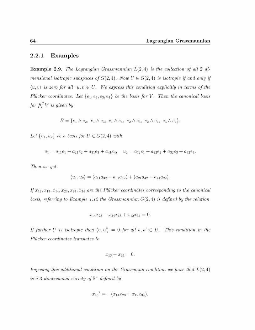
64 Lagrangian Grassmannian
2.2.1 Examples
Example 2.9. The Lagrangian Grassmannian L(2, 4) is the collection of all 2 di-
mensional isotropic subspaces of G(2, 4). Now U ∈ G(2, 4) is isotropic if and only if
〈u, v〉 is zero for all u, v ∈ U . We express this condition explicitly in terms of the
Plucker coordinates. Let e1, e2, e3, e4 be the basis for V . Then the canonical basis
for∧2 V is given by
B = e1 ∧ e2, e1 ∧ e3, e1 ∧ e4, e2 ∧ e3, e2 ∧ e4, e3 ∧ e4.
Let u1, u2 be a basis for U ∈ G(2, 4) with
u1 = a11e1 + a21e2 + a31e3 + a41e4, u2 = a12e1 + a22e2 + a32e3 + a42e4.
Then we get
〈u1, u2〉 = (a11a32 − a31a12) + (a21a42 − a41a22).
If x12, x13, x14, x23, x24, x34 are the Plucker coordinates corresponding to the canonical
basis, referring to Example 1.12 the Grassmannian G(2, 4) is defined by the relation
x14x23 − x24x13 + x12x34 = 0.
If further U is isotropic then 〈u, u′〉 = 0 for all u, u′ ∈ U . This condition in the
Plucker coordinates translates to
x13 + x24 = 0.
Imposing this additional condition on the Grassmann condition we have that L(2, 4)
is a 3-dimensional variety of P4 defined by
x132 = −(x14x23 + x12x34).

2.3 The number of points in L(n, 2n)(Fq) 65
2.3 The number of points in L(n, 2n)(Fq)
Lemma 2.10. The symplectic group Sp2n(k) acts transitively on the set of all isotropic
subspaces of G(n, 2n)(k), i.e. on the Lagrangian Grassmannian. In other words given
L1, L2 in L(n, 2n) there exists φ ∈ Sp(V ) such that
φ(V1) = V2.
Proof. This is a consequence of a special case of a theorem of Witt. For the details
refer to [2, Theorem 1.26 and Corollary 1.27].
By the above theorem we have
|L(n, 2n)(Fq)| =|Sp2n(Fq)|
|Stabilizer of X|for X ∈ L(n, 2n).
To find |Sp(2n)(Fq)| we use the following result from linear algebra.
Lemma 2.11. [21, p. 373− 374] If f is a symplectic form on a 2n-dimensional vector
space V over a field of q elements then the number of pairs u, v such that f(u, v) =
〈u, v〉 = 1 is (q2n − 1)q2n−1.
Proposition 2.12. The number of points of Sp2n(Fq) is given by
|Sp2n(Fq)| = qn2n∏
i=1
(qi − 1)(qi + 1).
Proof. Given a symplectic form f on vector space V of dimension 2n by standard
results there exists a symplectic basis v1, v2, · · · , v2n for V such that
〈vi, vi+n〉 = 1 for i = 1, · · · , n and 〈vi, vj〉 = 0 for |i− j| 6= n.
If vi is a symplectic basis of V then θ ∈ Sp(V ) if and only if θvi is also a symplectic
basis for V [21, p.336]. Therefore we have
〈θvi, θvi+n〉 = 1 for i = 1, . . . , n and 〈θvi, θvj〉 = 0 for |i− j| 6= n.
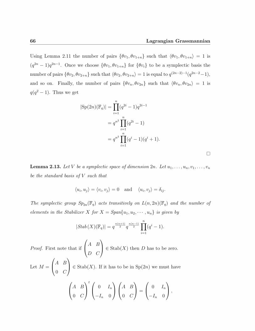
66 Lagrangian Grassmannian
Using Lemma 2.11 the number of pairs θv1, θv1+n such that 〈θv1, θv1+n〉 = 1 is
(q2n − 1)q2n−1. Once we choose θv1, θv1+n for θvi to be a symplectic basis the
number of pairs θv2, θv2+n such that 〈θv2, θv2+n〉 = 1 is equal to q(2n−2)−1(q2n−2−1),
and so on. Finally, the number of pairs θvn, θv2n such that 〈θvn, θv2n〉 = 1 is
q(q2 − 1). Thus we get
|Sp(2n)(Fq)| =n∏
i=1
(q2i − 1)q2i−1
= qn2n∏
i=1
(q2i − 1)
= qn2n∏
i=1
(qi − 1)(qi + 1).
Lemma 2.13. Let V be a symplectic space of dimension 2n. Let u1, . . . , un, v1, . . . , vn
be the standard basis of V such that
〈ui, uj〉 = 〈vi, vj〉 = 0 and 〈ui, vj〉 = δij.
The symplectic group Sp2n(Fq) acts transitively on L(n, 2n)(Fq) and the number of
elements in the Stabilizer X for X = Spanu1, u2, · · · , un is given by
|Stab (X)(Fq)| = qn(n+1)
2 qn(n−1)
2
n∏i=1
(qi − 1).
Proof. First note that if
A B
D C
∈ Stab(X) then D has to be zero.
Let M =
A B
0 C
∈ Stab(X). If it has to be in Sp(2n) we must have
A B
0 C
t 0 In
−In 0
A B
0 C
=
0 In
−In 0
,

2.3 The number of points in L(n, 2n)(Fq) 67
that is 0 AtC
−CtA BtC − CtB
=
0 In
−In 0
.
Thus we get, C = (A−1)tand BtC = CtB, i.e., CtB is a symmetric matrix. So M is
of the form
M =
A AS
0 (A−1)t
for some symmetric n × n matrix S. Let MSym
n be the group of symmetric n × n
matrices. Consider the maps Φ1 : GL(n) → Sp(2n) and Φ2 : MSymn → Sp(2n) given
by
Φ1(A) =
A 0
0 (A−1)t
and Φ2(S) =
I S
0 I
.
Then Φ1 and Φ2 are homomorphisms and
Φ1(A).Φ2(S) =
A 0
0 (A−1)t
In S
0 In
=
A AS
0 (A−1)t
.
We have Im (φ1)∩ Im (φ2) = I. It can be checked that Stab (X) is the semidi-
rect product of GL(n), the general linear n × n group, and M symn , the group of
symmetric n× n matrices. Therefore, we get
|Stab (X)(Fq)| = |M symn (Fq)| · |GL(n)(Fq)| = q
n(n+1)2
n−1∏i=0
(qn − qi)
= qn(n+1)
2 qn(n−1)
2
n∏i=1
(qi − 1).

68 Lagrangian Grassmannian
Proposition 2.14. The number of points in L(n, 2n)(Fq) is given by
|L(n, 2n)(Fq)| =n∏
i=1
(1 + qi).
Proof. The proof follows immediately from Proposition 2.12 and Lemma 2.13. We
have
|L(n, 2n)(Fq)| =|Sp2n(Fq)|
|GL(n)(Fq)|.|Sn(Fq)|=
qn2 ∏ni=1(q
i − 1)(qi + 1)
qn(n+1)
2 qn(n−1)
2
∏ni=1(q
i − 1)
=n∏
i=1
(1 + qi).
2.3.1 The Zeta function of the Lagrangian Grassmannian
The Lagrangian Grassmannian L(n, 2n) is a smooth projective subvariety of the
Grassmannian G(n, 2n) and we may consider it over any finite field Fq. By using
Proposition 2.14, the number of points in L(n, 2n)(Fq) is given by
|L(n, 2n)(Fq)| =n∏
i=1
(1 + qi).
As there are no terms in the denominator, Nr is a polynomial in powers of qr and the
Zeta function of such Grassmannians is easy to calculate.
Example 2.15. The Lagrangian Grassmannian L(2, 4)⊗Fq. By Proposition 2.14 we
have |L(2, 4)(Fq)| = (1+ q)(1+ q2) and so, Nr = 1+ qr + q2r + q3r = 1+ qr + q2r + q3r.
We get,
Z(L(2, 4)⊗ Fq, t) =1
(1− t)(1− qt)(1− q2t)(1− q3t).
Example 2.16. The Lagrangian Grassmannian L(3, 6)⊗ Fq. We have
|L(3, 6)(Fq)| = (1 + q)(1 + q2)(1 + q3),

2.3 The number of points in L(n, 2n)(Fq) 69
therefore we get, Nr = 1 + qr + q2r + 2q3r + q4r + q5r + q6r, and
Z(L(3, 6)⊗ Fq, t) =1
(1− t)(1− qt)(1− q2t)(1− q3t)2(1− q4t)(1− q5t)(1− q6t).
Theorem 2.17. The Zeta function of the Lagrangian Grassmannian L(n, 2n) is given
by
Z(L(n, 2n)⊗ Fq, t) =1
(1− t)(1− qt)b1(1− q2t)b2 . . . (1− qmt)bm,
where bi is equal to the number of strict partitions of i whose parts do not exceed n
and m = n(n+1)2
.
Proof. By Proposition 2.14 we get,
|L(n, 2n)(Fqr)| =n∏
i=1
(1 + qir).
For simplicity set qr = l. Then
Nr = |L(n, 2n)(Fqr)| =n∏
i=1
(1 + li) = (1 + l)(1 + l2) . . . (1 + ln) =m∑
i=0
bili
where the coefficient bi is equal to the number of strict partitions of i whose parts do
not exceed n and m = n(n+1)2
. So the coefficients bi can be calculated precisely and
one observes that the Zeta function in the general case is given by
Z(L(n, 2n)⊗ Fq, t) =1
(1− t)(1− qt)b1(1− q2t)b2 . . . (1− qmt)bm,
where bi and m are described as above.
We observe that the odd Betti numbers of the Lagrangian Grassmannian are zero.
2.3.2 Euler characteristic of the Lagrangian Grassmannian
Consider the Lagrangian Grassmannian L(n, 2n). Referring to the last section the
odd Betti numbers of the Lagrangian Grassmannian are zero and the even Betti
numbers satisfyn∏
i=1
(1 + li) =m∑
i=0
bili

70 Lagrangian Grassmannian
where m = n(n+1)2
is the dimension of L(n, 2n). Putting l = 1 in the above expression
we immediately get the Euler characteristic of the Lagrangian Grassmannian as
E =m∑
i=0
bi =m∏
i=1
(1 + 1i) = 2n.
2.4 Schubert calculus for Lagrangian Grassman-
nian
Definition 2.18. We denote a partition by λ = (λ1, λ2, . . . , λl). Thus λi are integers
and we agree that λ1 ≥ λ2 ≥ · · · ≥ λl ≥ 0. Hence λ is strict if λ1 > λ2 > · · · > λl > 0.
We define the length of λ by l(λ) = Card p | λp 6= 0 and the weight of λ by
|λ| =∑l
p=1 λp. By ρ(n) we mean the partition (n, n− 1, · · · , 2, 1). We denote by Dn
the set of all strict partitions λ with λ1 ≤ n.
Definition 2.19. Let F : 0 ⊂ F1 ⊂ F2 ⊂ · · · ⊂ Fn ⊂ V be a fixed flag of isotropic
subspaces of V such that dim Fi = i, ∀i = 1, 2, · · · , n. Such a flag is called a
complete isotropic flag of V .
Here Fn is an isotropic subspace of V of dimension n, so it is Lagrangian. In other
words, a complete isotropic flag is nothing but a Lagrangian subspace Fn together
with a complete flag of subspaces of Fn.
Note that any isotropic flag F : 0 ⊂ F1 ⊂ F2 ⊂ · · · ⊂ Fn ⊂ V can be completed
to a complete flag in V by setting Fn+i = F⊥n−i for 1 ≤ i ≤ n.
Definition 2.20. Let λ ∈ Dn, i.e., let λ = (λ1 > λ2 > · · · > λl > 0) be any strict
partition with λ1 ≤ n. Let F : 0 ⊂ F1 ⊂ F2 ⊂ · · · ⊂ Fn ⊂ V be a complete isotropic
flag of V . With respect to this flag and partition we define the Schubert variety
in the Lagrangian case as
Xλ = Xλ(F) := L ∈ L(n, 2n) | dim(L ∩ Fn+1−λi) ≥ i, 1 ≤ i ≤ l(λ).

2.4 Schubert calculus for Lagrangian Grassmannian 71
It can be shown that Xλ actually defines a complex projective variety of codi-
mension |λ| in L(n, 2n). The variety Xλ determines a Schubert class Ω(λ) = [Xλ]
in the cohomology group H2|λ|(L(n, 2n); Z). The Schubert classes Ω(i) = σ(i) for
i = 1, 2, · · · , n (i.e. l = 1, λ1 = i) are called special (they parametrize isotropic n-
planes such that dim(L⋂Fn+1−i) ≥ 1. For the details of the subject our main
reference is [22, p.1− 4]. As before we define the cohomology ring H∗(L(n, 2n),Z) of
the Lagrangian Grassmannian as the direct sum⊕
i≥0Hi(L(n, 2n); Z).
Theorem 2.21. [22, p.2] The cohomology group H∗(L(n, 2n),Z) is a free abelian
group and the Schubert classes Ω(λ), λ ∈ Dn, form an additive basis for the cohomol-
ogy ring H∗(L(n, 2n),Z). We have an isomorphism of abelian groups
H∗(L(n, 2n),Z) =⊕λ∈Dn
Z · Ω(λ),
where the sum varies over all strict partitions λ = (λ1 > λ2 > · · · > λl > 0) with
λ1 ≤ n.
2.4.1 Cohomology groups of the Lagrangian Grasmannian
We now calculate the dimensions of the cohomology groups of some Lagrangian Grass-
mannians. Using Theorem 2.21 and definition 2.20 we see that the codimension k
classes of the Lagrangian Grassmannian are indexed by strict partitions of the form
λ : (λ1 > λ2 > · · · ≥ 0) with λ1 ≤ n and weight of λ equal to k. So the k-th Betti
number of L(n, 2n) is equal to the number of such strict partitions.
Example 2.22. The Lagrangian Grassmannian L(2, 4). The dimension of the coho-
mology group H2k(L(2, 4); Z) equals the number of strict partitions λ such that 2 ≥ λ1
and |λ| = k for k = 0, · · · , 3.

72 Lagrangian Grassmannian
Codimension k admissible partitions dim(H2k(L(2, 4); Z))
0 0 1
1 1 1
2 2 1
3 (2, 1) 1
Example 2.23. The Lagrangian Grassmannian L(3, 6). The dimension of the coho-
mology group H2k(L(3, 6); Z) equals the number of strict partitions λ such that 3 ≥ λ1
and |λ| = k for k = 0, · · · , 6.
Codimension k admissible partitions dim(H2k(L(3, 6); Z))
0 0 1
1 1 1
2 2 1
3 (2, 1), 3 2
4 (3, 1) 1
5 (3, 2) 1
6 (3, 2, 1) 1
Example 2.24. The Lagrangian Grassmannian L(4, 8): The dimension of the coho-
mology group H2k(L(4, 8); Z) equals the number of strict partitions λ such that 4 ≥ λ1
and |λ| = k for k = 0, · · · , 10.

2.5 Representability of Lagrangian Grassmann functor 73
Codimension k admissible partitions dim(H2k(L(4, 8); Z))
0 0 1
1 1 1
2 2 1
3 (2, 1), 3 2
4 4, (3, 1) 2
5 (4, 1), (3, 2) 2
6 (4, 2), (3, 2, 1) 2
7 (4, 3), (4, 2, 1) 2
8 4, 3, 1 1
9 4, 3, 2 1
10 4, 3, 2, 1 1
By these examples we see that the dimensions of the cohomology groups match
with the Betti numbers of the Lagrangian Grassmannians calculated before.
2.5 Representability of Lagrangian Grassmann func-
tor
Let n be any positive integer. For a ring T consider the standard symplectic form
on the T -module T 2n. We call a submodule K of T 2n isotropic if the standard
symplectic form vanishes on it. The Lagrangian Grassmann functor is a functor
l : (rings) → (sets) is given by
l(T ) = isotropic T -submodules K ⊂ T 2n that are rank n direct summands of T 2n
We will use theorem 1.51 to show that l is representable. We need to show that
1. l is a sheaf in the Zariski topology.

74 Lagrangian Grassmannian
2. There exist rings Ri and elements Wi ∈ l(Ri) such that for every field F , l(F )
is the union of images of hRi(F ) under the maps Wi : hRi
→ l.
We first show that l is a sheaf in the Zariski topology. The proof proceeds as in the
case of the classical Grasmann functor except for a few modifications. If f : R1 → R2
is a ring homomorphism the corresponding morphism f : l(R1) → l(R2) is given by
f(V ) = V ⊗R1 R2.
Note that if V is an isotropic rank n summand of R2n1 then V ⊗R1 R2 is isotropic rank
n summand of R2n2 . Suppose that we have a nondegenerate alternate pairing
< , > : R2n1 ×R2n
1 → R1.
Then f extends linearly and we get a pairing
< , > , : R2n2 ×R2n
2 → R2.
If V ⊂ R2n1 is isotropic, 〈v, v′〉 = 0 for all v, v′ ∈ V . Then for vi, v
′i ∈ V and ri, r
′i ∈ R2
we have ⟨∑i
v1 ⊗ ri,∑
j
v′j ⊗ r′j
⟩=∑i,j
rir′j
⟨vi, v
′j
⟩= 0.
Therefore, V ⊗R1 R2 is an isotropic summand of R2n2 .
We now show that l is a sheaf in the Zariski topology. Let R be a ring. Let
X = SpecR. Consider the open covering of X by distinguished open affine sets
Ui = SpecRfi. Suppose that for every collection of elements Wi ∈ l(Rfi
), Wi and Wj
map to the same element in l(Rfifj). So in l(Rfifj
) let
Wi ⊗RfiRfifj
= Wj ⊗RfjRfifj
.
We wish to show that there exists a unique element W ∈ l(R) that maps to each
of the Wi. We can construct the required isotropic direct summand W exactly as in

2.5 Representability of Lagrangian Grassmann functor 75
the classical case (for details refer to section 1.4.1). Such a W exists uniquely and is
defined by
W = w ∈ Rn | w ∈ Rnfi, w ∈ Wi for all i.
Since Wi ∈ l(Rfi) are isotropic for all i and W is contained in Wi for all i we see that
the summand W is also isotropic. Thus, l is a sheaf in the Zariski topology. Now we
have to show that there exist rings Ri and elements Wi ∈ l(Ri) such that for every
field F , l(F ) is the union of images of hRi(F ) under the maps Wi : hRi
→ l. Let
r =(2nn
)− 1. Let g(n, 2n) := g : (rings) → (sets) be the Grassmann functor given by
g(T ) = T -submodules K ⊂ T 2n that are rank n direct summands of T 2n.
Let PrZ = Proj [. . . , XI , . . . ] be the projective space with homogeneous coordinates
XI corresponding to the subsets of cardinality n in 1, 2, . . . , 2n. Recall that the
projective scheme PrZ comes from the functor
hPrZ(T ) = Mor (SpecT,Pr
Z)
= T -submodules K ⊂ T r+1 that are rank r direct summands of T r+1
We now refer to the section 1.4.2. With the same notations of section 1.4.2, replacing
d by n and n by 2n we get,
UI(T ) ∩ ι(g(T )) =
rank n summands K ⊂ T 2n such that eI generates
T r+1
(∧nK)⊥
= K ⊂ T 2n |K = Spv1, . . . , vnwith 〈v1 ∧ · · · ∧ vn, eI〉 ∈ T ∗.
Thus we see that UI(T ) ∩ ι(l(T )) is given byisotropic rank n summands K ⊂ T 2n such that eI generates
T r+1
(∧nK)⊥
,
which is equal to
K ⊂ T 2n | K isotropic spanned by v1, . . . , vn, 〈v1 ∧ · · · ∧ vn, eI〉 ∈ T ∗.

76 Lagrangian Grassmannian
By Lemma 1.57 we see that for a direct summand K ⊂ T 2n spanned by v1, . . . , vn,
〈v1 ∧ · · · ∧ vn, eI〉 ∈ T ∗ if and only if the image of K via the Plucker map i.e. P (K)
is in UI . Let U be the complemetary subspace of K. If further K is isotropic then
we see from section 2.2 that the affine neighbourhood UI of K is isomorphic to
ϕ : K → U | ϕ = ϕ∗ = HomSym(K,U) ∼= An(n+1)
2T .
Therefore UI
⋂ι(l) is represented by affine scheme A
n(n+1)2 = Spec Z[(xi), i = 1, · · · , n(n+1)
2].
Then taking Ri as Z[xi] we see that for any field F
g(F ) =⋃
(UI ∩ i(l))(F ).
Therefore the second condition in Theorem 1.51 is satisfied by the Lagrangian Grass-
mann functor. Thus the Lagrangian Grassmann functor is representable.
Computation of the Zeta function of L(n, 2n) using Schubert calculus
Note that the Zeta function of L(n, 2n) can also be computed using Schubert calculus.
The Lagrangian Grassmannian can be considered over fields of characteristic zero
namely Q, C and also over finite field Fq. Exactly following section 1.4.3 we have for
X = L(n, 2n) the following isomorphisms
H iet(X ⊗Q; Ql) ∼= H i
et(X ⊗ C; Ql) ∼= H iBetti(X ⊗ C; Ql) ∼= H i
Betti(X ⊗ C; Z)⊗Z Ql.
Then with the Basis Theorem of the Schubert calculus in Lagrangian case (Theorem
2.21), the Zeta function of L(n, 2n) can be computed as in section 1.4.3 which comes
out to be
Z(L(n, 2n), t) =1∏m
i=0(1− pit)b2i,
where m is the dimension of the Lagrangian Grassmannian and b2i denotes the rank of
H2i(L(n, 2n); Z) over Z. This agrees with the calculations done before in section 2.3.1.

2.5 Representability of Lagrangian Grassmann functor 77
2.5.1 The Zeta function of the Lagrangian Grassmann Scheme
Theorem 2.25. The Zeta function of the Lagrangian Grassmann scheme LZ(d, n) is
a product of Riemann Zeta functions given by
ζ(LZ(n, 2n), s) =m∏
i=0
ζbi(s− i),
where m is the dimension of L(n, 2n).
Proof. Consider the Lagrangian Grassmann scheme LZ(d, n). Let us assume that
m = dimL(n, 2n) = n(n+1)2
. The Z(LZ(n, 2n)⊗ Fp, t) is given by
Z(LZ(n, 2n)⊗ Fp, t) =1
(1− t)b0(1− pt)b1 . . . (1− pmt)bm,
where the Betti number bi equals the number of strict partitions of i whose parts do
not exceed n. Then referring to section 1.4.4, ζ(LZ(n, 2n), s) is given by
ζ(LZ(n, 2n), s) =∏
p
ζ(LZ(n, 2n)⊗ Fp, s) =∏
p
Z(LZ(n, 2n)⊗ Fp, p−s)
=∏
p
1
(1− t)b0(1− pt)b1 . . . (1− pmt)bmwhere t = p−s
=m∏
i=0
ζbi(s− i).
Thus, we see that ζ(LZ(d, n), s) can be expressed as a product of the Riemann Zeta
functions.

78 Lagrangian Grassmannian

79
Chapter 3
Other subschemes of the
Grassmannian
In Chapter 1 we saw that the usual Grassmannian G(d, n) can be considered as a
scheme over Spec Z. The Grassmann scheme G = GZ(d, n) represents the Grassmann
functor g : (rings) → (sets) given by
g(T ) = T -submodules K ⊂ T n that are rank d direct summands of T n.
By the results of Chapter 1 the Grassmann schemeG = GZ(d, n) is a closed subscheme
of the projective space PrZ where r =
(nd
)− 1. It is a smooth projective variety over
Spec Z of relative dimension d(n − d). Moreover the Grassmannian G(d, n) has a
covering by spaces each isomorphic to affine space Ad(n−d).
In Chapter 2 we saw that the Lagrangian Grassmann scheme L = LZ(n, 2n)
represents the Lagrangian Grassmann functor l : (rings) → (sets) given by
l(T ) = isotropic T -submodules K ⊂ T 2n that are rank n direct summands of T 2n.
The Lagrangian Grassmann scheme L is a closed subscheme of PrZ where r is given
by r =(2nn
)− 1. It is a smooth projective variety over Spec Z of relative dimension

80 Other subschemes of the Grassmannian
n(n+ 1)
2. Moreover the Lagrangian Grassmannian has a covering by spaces each
isomorphic to affine space An(n+1)
2 .
Now fix a ring R ⊂ Mn(Z) and an integer, 0 < d < n. Let fR : (rings) → (sets)
be the functor such that fR(T ) is
T -submodules K ⊂ T n that are R-invariant rank d direct summands of T n,
where we say that a summand K ⊂ T n is R-invariant if r.a ∈ K for all r in R and
for all a ∈ K. In this Chapter we prove that fR is represented by a closed scheme
FR ⊂ GZ(d, n). Moreover we provide an explicit affine covering of FR.
We focus on the following case. Let R be the ring of integers of a number field Q.
Let [Q : Q] = d and n = 2d. The embedding R ⊂ M2d(Z) can be chosen as follows.
The ring R acts diagonally on R ⊕ R by r(r1, r2) = (rr1, rr2) . If R =⊕d
i=1 Zvi as
groups then R ⊕ R ∼= Z2d. We study below the local structure of FR and its Zeta
function in some particular cases. Our motivation is the following.
Suppose k is an algebraically closed field and A is an abelian variety over Spec k
of dimension d. Let Ck denote the category of local Artinian rings (B,m) such that
B/m = k. Let δ : Ck → (sets) be the deformation functor given by
δ(B) = (A, φ) | A/SpecB an abelian scheme,φ : A⊗B (B/m) ∼= A / ∼=
Theorem 3.1. (Grothendieck, de Jong, Deligne - Pappas, others) There exists a com-
plete local noetherian ring D with residue field k that pro-represents δ; for any ringB
in Ck, δ(B) = Homcont(D,B). Moreover there is a k- rational point, say x, of the
Grassmannian G(n, 2n) such that
D ∼= OG,x∼= SpecW (k)[[x1, x2, . . . , xd(n−d)]]
(if k has characteristic 0 we can replace W (k) by k).

3.1 Representability of the functor fR 81
In general, deformations of abelian varieties possibly provided with extra data such
as an embedding R ⊂ End(A) or a principal polarization are related to completed
local rings on the Grassmannian FR or L. In particular we have the following theorem.
Theorem 3.1.(continued) Let R be a ring of integers. Let (A, i) be an abelian variety
over k with an embedding i : R → Endk(A). Let δR : Ck → (sets) be the deformation
functor given by
δR(B) =
(A, I, φ) | A/ SpecB is an abelian scheme,
I : R→ EndB(A), φ : A⊗B (B/m) ∼= A, I induces i
.
Then δR is represented by a complete local noetherian ring DR with residue field k
and moreover DR∼= OFR,x, the completion of the local ring of the Grassmannian FR
at a suitable point x.
3.1 Representability of the functor fR
Recall that for a fixed ring R ⊂Mn(Z) and an integer 0 < d < n, fR(T ) is given by
T -submodules K ⊂ T n that are R-invariant rank d direct summands of T n.
Let W be a free rank d submodule of T n which is R-invariant. We first show that fR
is a sheaf in the Zariski topology. Let T be a ring. Let X = SpecT . Consider the
open covering of X by distinguished open affine sets Ui = SpecTfi. Suppose for every
collection of elements Wi ∈ fR(Tfi), Wi and Wj map to the same element in fR(Tfifj
).
So in fR(Tfifj) we have
Wi ⊗TfiTfifj
= Wj ⊗TfjTfifj
.
We wish to show that there exists a unique element W ∈ fR(T ) that maps to each
of the Wi. The existence and uniqueness part follows from the case of the Grass-
mann functor. We have to verify that if Wi are R-invariant for all i then the direct

82 Other subschemes of the Grassmannian
summand W as obtained in the section 1.4.2 is also R-invariant. Referring to section
1.4.2 we get a rank d direct summand W of T n as
W = Γ(X,F) = w ∈ T n | w ∈ T nfi, w ∈ Wi for all i.
Now if r ∈ R and w ∈ W we see that w ∈ Wi for all i and as each Wi is R-invariant,
r · w ∈ Wi. It follows that r · w ∈ W . Thus W is R-invariant.
Now let W be a rank d summand of T n. Suppose we have a splitting of T n as
T n = W ⊕U where U is a rank (n−d) free submodule of T n. Then we have an affine
neighbourhood of W namely, Hom[R](W,U) ⊂ Hom(W,U) given by
Hom[R](W,U) = ϕ : W → U | Γϕ is R- invariant.
Lemma 3.2. The subset Hom[R](W,U) ⊂ Hom (W,U) ∼= Ad(n−d) is closed.
Proof. We have Hom[R](W,U) =⋂
r∈R Hom[r](W,U) where by definition
Hom[r](W,U) = ϕ : W → U | Γϕ is r-invariant.
Let e1, . . . , ed be a basis for W . Then a basis for the graph of ϕ, Γϕ is given by
(ei, ϕ(ei)) | 1 ≤ i ≤ d. Extend the basis e1, . . . , ed of W to a basis of T n. We
have
Hom[R](W,U) =⋂r∈R
d⋂i=1
Hom[r],i(W,U)
=⋂r∈R
d⋂i=1
ϕ : W → U | r(ei, ϕ(ei)) ∈ Γϕ.
Let Mi be a n × (d + 1) matrix with the first d colums given by ei + ϕ(ei) for
i = 1, · · · , d and the (d+ 1)-th column given by r(ei + ϕ(ei)). Then r(ei, ϕ(ei)) ∈ Γϕ
if and only if all the (d + 1) × (d + 1) determinants of the matrix Mi vanish. This
defines a closed condition. Thus each Hom[r],i(W,U) is a closed set in Hom(W,U) and
Hom[R](W,U) is a closed subset of Hom(W,U) being a intersection of closed sets.

3.2 Properties of FR 83
Corollary 3.3. The functor fR is representable.
Proof. By the above discussion we see that the functor fR is a sheaf in the Zariski
topology. Also by Lemma 3.2, given W a rank d summand which is R-invariant and
complementary submodule U , we have a neighbourhood of W , namely
Hom[R](W,U) ⊂ Hom (W,U) ∼= Ad(n−d).
Then referring to Theorem 1.51 it follows that the functor fR is representable.
Now, let V be a vector space of dimension n over an algebraically closed field k.
Suppose a ring R acts on V . Let W be a rank d direct summand of V that is R-
invariant. Suppose we have a splitting V = W ⊕U . Then U = V/W has a R-module
structure. Note that U as a subspace of V may not be R-invariant. In general, the
set
Γϕ | ϕ : W → U , ϕ is a k-linear map with Γϕ R-invariant
is not same as the set HomR⊗k(W,U). However we will see that HomR⊗k(W,U) is in
natural bijection with the tangent space to the scheme FR at W .
3.2 Properties of FR
In this section we will give a description of the Zariski tangent space to the Gras-
mannian G(d, n) at a k-valued point. Hence we will describe the tangent space to the
scheme FR at a k-valued point W . Recall that if X is any scheme, then for any k-
rational point x ∈ X the Zariski tangent space Tx to X at x is Hom(m/m2, k), where
m = mX,x is the maximal ideal in the local ring of X at x and k is the residue field
of X at x. Now suppose that X is a scheme over field k. Then to give a k morphism
of Spec k[ε]/(ε2) to X is equivalent to giving a point x ∈ X, rational over k (i.e.
k(x) = k), and an element of Tx. For the details refer to [6, p.256-257].

84 Other subschemes of the Grassmannian
Proposition 3.4. The Zariski tangent space to the Grassmannian G(d, n) at a k-
valued point W is isomorphic to Homk(W, kn/W ).
Proof. If W is a k-valued point of the Grassmannian G(d, n) it is a rank d summand
of kn. Let k[ε] = k(ε)/(ε2). By the above discussion, to give a tangent vector to
G(d, n)(k) at W is to giving a k-morphism k[ε] → G(d, n)(k), i.e. by section 1.4.2 of
Chapter 1, giving a rank d direct summand of k[ε]n which reduces to W mod ε. Thus,
the Zariski tangent space to G(d, n)(k) at W is the set of all rank d summands M of
k[ε]n which reduce to W modulo ε. We now show that the collection of all such M
can be identified with Homk(W, kn/W ). Let first M be a rank d summand of k[ε]n
that is W modulo ε. Then M ⊗k[ε] k = W , and we get an exact sequence
0 → εM →M → W → 0
We have εM = εW , and for all w ∈ W there is a ϕ(w) ∈ kn, such that w+ϕ(w)ε ∈M .
Using this and the fact that the above sequence is exact, the module M has the form
M = w + ϕ(w)ε | w ∈ W+ εW.
Then ϕ gives a map W → kn/W . Moreover, if w1, w2 ∈ W , we have
([w1 + ϕ(w1)ε] + [w2 + ϕ(w2)ε]− [w1 + w2 + ϕ(w1 + w2)ε]) ∈ εW.
Therefore, we have
ϕ(w1) + ϕ(w2)− ϕ(w1 + w2) ∈ W,
which implies ϕ(w1) + ϕ(w2)− ϕ(w1 +w2) is zero in kn/W . Similarly, one finds that
ϕ(aw)−aϕ(w) ∈ W for all w ∈ W and a ∈ k. Thus, the map ϕ defines a k-linear map
W → kn/W . Also, if ψ : W → kn/W is another function such that for all w ∈ W ,
(w + ψ(w)ε) ∈M then
ϕ(w)ε− ψ(w)ε ∈M ⇒ ϕ(w)− ψ(w) ∈ W.

3.2 Properties of FR 85
Thus ϕ(w) − ψ(w) is zero in kn/W and ϕ = ψ. So, given a rank d summand M of
k[ε]n that is W modulo ε we get a well defined map in Homk(W, kn/W ). Now let
ϕ : W → kn/W be a k-linear map. We want to define a rank d summand M of k[ε]n
that is W modulo ε. Lift ϕ to a map ϕ : W → kn. Define M by
M = w + ϕ(w)ε | w ∈ W+ εW.
Then M is closed under addition, closed under multiplication by elements in k[ε] and
is independent of the choice of ϕ. So M is a k[ε] module that is W modulo ε and has
rank d as W has rank d, and M is the required summand.
Corollary 3.5. The Zariski tangent space to the scheme FR at a k-valued point W
is isomorphic to HomR⊗k(W, kn/W ).
Proof. If W is a k-valued point of FR it is an R- invariant rank d summand of kn.
By the above proposition the Zariski tangent space to FR at W is the set of all R-
invariant rank d summands M of k[ε]n that reduce to W modulo ε. Suppose first
that M is R-invariant. So we get a k linear map ϕ ∈ Homk(W, kn/W ). Then for
r ∈ R, w ∈ W we have
r(w + ϕ(w)ε) ∈M and rw + ϕ(rw)ε ∈M.
Therefore,
(rϕ(w)− ϕ(rw))ε ∈M ⇒ rϕ(w)− ϕ(rw) ∈ W.
Thus rϕ(w)−ϕ(rw) is zero in kn/W and we get that ϕ is R-linear. Conversely if we
have a R-linear map ϕ : W → kn/W then for r ∈ R, ϕ(rw) = r(ϕ(w)). So for the
corresponding lift ϕ : W → kn, ϕ(rw) = r(ϕ(w)) modulo W . Therefore the module
M = w + ϕ(w)ε | w ∈ W+ εW,
as defined in the above theorem, is R-invariant.

86 Other subschemes of the Grassmannian
Example 3.6. Suppose k is an algebraically closed field. Let R ⊗ k = k[ε]. Suppose
V = k[ε]2, W = k[ε], U = k[ε] and V = W ⊕ U . Then
HomR⊗k(W,U) = Homk[ε](k[ε], k[ε]) ∼= k[ε],
which is 2-dimensional over k. However, if W = (ε)⊕ (ε), then V/W ∼= (ε)⊕ (ε) as
k[ε] modules and the tangent space to W as a point on FR is given by
Homk[ε](W,U) = Homk(W,U),
which is four dimensional. Thus W , as a point on FR, is singular.
Proposition 3.7. Let V be a vector space over an algebraically closed field k. Suppose
a ring R acts on V . Assume that V = W ⊕ U where W and U are R-invariant. Let
ϕ : W → U be a k-linear homomorphism. Then the graph of ϕ, Γϕ is R-invariant
if and only if ϕ is R-equivariant. Thus an affine neighbourhood of FR is given by
HomR⊗k(W,U).
Proof. Let Γϕ be R-invariant. Let r ∈ R, w ∈ W . Then (w,ϕ(w)) ∈ Γϕ implies
(rw, rϕ(w)) and (rw, ϕ(rw)) belong to Γϕ. Thus r(ϕ(w)) = ϕ(rw) and so ϕ is R-
equivariant. Conversely suppose that ϕ is R-equivariant. Let (w,ϕ(w)) ∈ Γϕ. Then
for r ∈ R
r(w,ϕ(w)) = (rw, r(ϕ(w))) = (rw, ϕ(rw)) ∈ Γϕ.
Hence, Γϕ is R-invariant.
Let T be any algebraically closed field. Let R be the ring of integers of a number
field Q(R) with [Q(R) : Q] = d. Assume that R⊗ T is a sum of fields, say
R⊗Z T =⊕
α
T ∼= T d,
where the sum varies over all ring homomorphisms α : R→ T . To give a T -submodule
M ⊂ T 2d of rank d that is R-invariant is same as giving a R⊗T invariant submodule
of (R⊗Z T )2 of rank d over T .

3.2 Properties of FR 87
Lemma 3.8. Let R and T be as above. Let M ⊂ (R⊗ T )2 be a submodule of rank
d over T . Then M is R ⊗ T invariant if and only if M =⊕d
i=1Mi, where Mi is a
T -submodule of T 2 of rank ri and∑d
i=1 ri = d.
Proof. Note that R and T are commutative rings with unity. Every submodule M of
(R⊗ T )2 can be written as
M =d⊕
i=1
eiM =d⊕
i=1
Mi,
where ei are the idempotents corresponding to the decomposition R ⊗ T =⊕
α T .
Each Mi is a T module of T 2. If M has rank d and Mi has rank ri then∑ri = d.
The invariants (r1, · · · , rd) are discrete invariants of the module M . We see that
the Grassmann variety FR⊗T is a disjoint union∐
r=(r1,··· ,rd) Vr, where the union is
over vectors (r1, · · · , rd) such that each 0 ≤ ri ≤ 2 and∑ri = d. The component Vr
parametrizes modules M with invariant r.
Now let M ⊂ (R⊗ T )2 be an R-invariant rank d summand of T 2d as a T -module.
Suppose T 2d = M ⊕ U where U is also R-invariant. Write M = ⊕Mi and U = ⊕Ui
where each Mi and Ui is a T -module. An affine neighbourhood of M in FR⊗T is given
by
HomR⊗T (M,U) = Γϕ | ϕ : M → U such that Γϕ is R⊗ T -invariant.
But, we have
HomR⊗T (M,U) =⊕
i
HomT (Mi, Ui).
Thus, for ϕ : W → U , the graph of ϕ, Γϕ, has the form
Γϕ =d⊕
i=1
Γϕi,
where each Γϕihas rank ri. We see that Vr equals j copies of P1 where j is number
of i such that ri = 1.
In the case when d = 2 we have following possibilities :

88 Other subschemes of the Grassmannian
1. Mi is 0 and Ui has rank 2.
2. Ui is 0 and Mi has rank 2.
3. Both Mi and Ui have rank 1
3.3 Example : Quadratic field
We now consider the following example of a quadratic field. Suppose L = Q(√D) is
a quadratic extension of Q where D is a squarefree integer. We have [L : Q] = 2. Let
R be the ring of integers in L. Then
R =
Z[√D] if D ≡ 2, 3 (mod 4);
Z[1+√
D2
] if D ≡ 1 (mod 4).
The discriminant dL of R is
dL =
4D if D ≡ 2, 3 (mod 4);
D if D ≡ 1 (mod 4).
Let k = Fp and R1 = R⊗ k. Consider R21 = R1 ⊕R1. It has two structures, namely:
1. R21 is an R1- module. For r1, r2, r ∈ R1 define r(r1, r2) = (rr1, rr2).
2. R21 is a k-vector space of dimension 4 i.e. R2
1∼= k4.
We are interested in a subscheme FR1(2, 4)(k) ⊂ G(2, 4)(k) which is the collection of
all 2-dimensional subspaces of R21 that are R1- invariant. We concentrate on the case
when D ≡ 2, 3 (mod 4). We have
R1 = R⊗ k =
Fp ⊕ Fp, Fp characteristic p, (p) inert in L;
Fp ⊕ Fp, Fp characteristic p, (p) split in L ;
Fp[t]/t2, Fp characteristic p, (p) ramified in L.

3.3 Example : Quadratic field 89
First two cases: If (p) is inert or spilt in L, R1 = Fp⊕Fp, R21 = (Fp⊕Fp)⊕(Fp⊕Fp).
We are interested in 2- dimensional subspaces of R21 that are R1-invariant. Note that
U is such a subspace if and only if U is preserved under (1, 0) and (0, 1). But
(0, 1) = (1, 1)− (1, 0).
So it is enough to consider the subspaces of R21 that are invariant under (1, 0). Let
e1 = (1, 0, 0, 0), e2 = (0, 1, 0, 0), e3 = (0, 0, 1, 0), e4 = (0, 0, 0, 1) be the standard
basis for k4. Let t : R21 → R2
1 be the linear transformation given by
t =
(1
01
0
)Then we are interested in 2-dimensional subspaces of R2
1 that are preserved under t.
The basis e1, e2, e3, e4 of R21 has the property that t acts as identity on e1, e3 and acts
as zero on e2, e4. Let M1 = spane2, e4, M2 = spane1, e3. Then R21 = M1⊕M2. If
N is a submodule of R21 of dimension 2 by Lemma 3.8 we can write it as N = N1⊕N2
where N1, N2 are submodules of M1,M2 respectively. If N has dimension 2 we have
the following three possibilities.
1. N = M1 = spane2, e4;
2. N = M2 = spane1, e3 ;
3. N= span a2e2 + a4e4, a1e1 + a3e3 | a2 6= 0 or a4 6= 0, and a1 6= 0 or a3 6= 0.
We now analyse these three cases. Let x12, x13, x14, x23, x24, x34 be the Plucker coor-
dinates corresponding to the canonical basis of∧2 k4. Then, referring to section 1.12
in Chapter 1, we see that the Grassmann relation satisfied by G(2, 4) is given by
x14x23 − x24x13 + x12x34 = 0.
1. When N = spane2, e4 its image under the Plucker map is the point in P5
given by (0 : 0 : 0 : 0 : 1 : 0). This is a closed subset of P5 defined by
Z1 = V x12, x13, x14, x23, x34.

90 Other subschemes of the Grassmannian
2. When N = spane1, e3 its image in P5 is (0 : 1 : 0 : 0 : 0 : 0) . This is a closed
subset of P5 defined by
Z2 = V x12, x14, x23, x24, x34.
3. Assume we are in the third case. Let v1 = a2e2 + a4e4, v2 = a1e1 + a3e3. Then
v1 ∧ v2 = (−a1a2)e1 ∧ e2 + (0)e1 ∧ e3 + (−a1a4)e1 ∧ e4
+ (a2a3)e2 ∧ e3 + (0)e2 ∧ e4 + (−a3a4)e3 ∧ e4.
So the Plucker coordinates of such N are
(−a1a2 : 0 : −a1a4 : a2a3 : 0 : −a3a4).
In addition to the Plucker relations these points in P5 satisfy the following
relations in the coordinates
x12x34 + x14x23 = 0, x13 = 0, x24 = 0.
Moreover, one checks that every point on the closed set of G(2, 4) defined by
those relations comes from some N . In fact the collection of all such points is
isomorphic to a quadratic surface in P3 defined by
Z3 = V x12x34 + x14x23
and so is isomorphic to P1 × P1 over Fp. This agrees with the discussion in the
previous section. However, since the isomorphism Z3∼= P1 × P1 is only over Fp,
we will use explicit equations below to compute the Zeta function.
We now compute the Zeta function of this Grassmannian FR1(2, 4)(k) contained
in G(2, 4)(k). Let σ : A4k → A4
k be the Frobenius morphism. The Galois group
Gal(Fp/Fp) acts on R1 = (R⊗ Fp) by
σ(l ⊗ λ) = l ⊗ σ(λ).
This action induces the action of the Galois group on R21. We want to see the action
of the Galois group on the Plucker coordinates.

3.3 Example : Quadratic field 91
3.3.1 The Zeta function : (p) inert in L
Assume that (p) is inert in L. Then
Z[√D]/(p) ∼= Fp[x]/(x
2 −D) =: F,
which is a field with p2 elements. There exist two embeddings τ1, τ2 : F → Fp and
R ⊗ Fp∼= F2
p by the map f : l ⊗ λ 7→ (τ1(l)λ, τ2(l)λ). Note that R = Z · 1 ⊕ Z[√D]
as a group and
f(1⊗ 1) = (1, 1), f(√D ⊗ 1) = (
√D,−
√D).
The elements (1, 1), (√D,√−D) form a basis to F2
p and the Frobenius morphism σ
acts on (1, 1) and (√D, 1) as the identity.
Let M =(
1√
D
1 −√
D
). Then M−1 = −1
2√
D
(−√
D −√
D−1 1
). The matrix M−1 changes
coordinates from the standard basis of F2
p to the basis (1, 1), (√D,√−D). Let
α = (α1, α2) be any general element of F2
p. Supposeλ1
λ2
= M−1
α1
α2
.
Then
λ1
λ2
=
α1+α2
2
α1−α2
2√
D
are the coordiantes of α in the basis (1, 1), (√d,√−d).
Therefore, we get
σ
λ1
λ2
=
σ(α1)+σ(α2)2
σ(α1)−σ(α2)
2σ(√
D)
=
σ(α1)+σ(α2)2
σ(α1)−σ(α2)
−2√
D
.
Now,
σ
α1
α2
= Mσ
λ1
λ2
=1
2
1√D
1 −√D
σ(α1) + σ(α2)
σ(α1)−σ(α2)
−√
D
=
σ(α2)
σ(α1)
.

92 Other subschemes of the Grassmannian
So σ acts on (α1, α2) ∈ k2 by
σ
α1
α2
=
σ(α2)
σ(α1)
.
Thus, σ acts on k4 by
σ(a1, a2, a3, a4) = (σ(a2), σ(a1), σ(a4), σ(a3)),
and it acts on the Plucker coordinates by
σ(x12) = −x12, σ(x13) = x24, σ(x14) = x23,
σ(x23) = x14, σ(x24) = x13, σ(x34) = −x34.
Now we come back to the subvariety of G(2, 4) defined by
x12x34 + x14x23 = 0, x13 = x24 = 0.
The points on this subvariety have Plucker coordinates (c12 : 0 : c14 : c23 : 0 : c34)
satisfying the relation c12c34 + c14c23 = 0. The Frobenius morphism σ acts on
(c12 : 0 : c14 : c23 : 0 : c34) by
σ(c12 : 0 : c14 : c23 : 0 : c34) = (−σ(c12) : 0 : σ(c23) : σ(c14) : 0 : −σ(c34)).
One has
σ2(c12 : 0 : c14 : c23 : 0 : c34) = (σ2(c12) : 0 : σ2(c14) : σ2(c23) : 0 : σ2(c34)).
In fact we see that if r is any even positive integer then σr acts by
σr(c12 : 0 : c14 : c23 : 0 : c34) = (σr(c12) : 0 : σr(c14) : σr(c23) : 0 : σr(c34)).
This action of σr is usual componentwise action as in case of projective spaces. So the
number of subspaces invariant under the action of σr is simply equal to the number
of solutions to x12x34 +x14x23 = 0 over Fq with q = pr. To count those we distinguish
two cases.

3.3 Example : Quadratic field 93
1. Suppose x12 6= 0. Each of x14 and x23 can be chosen arbitrarily. Hence each
of them has q choices and x34 is determined by x34 = −x14x23
x12
. So the total
number of solutions in this case is q2.
2. Suppose x12 = 0. Then either x14 = 0 or x23 = 0 or both of them are zero. The
total number of solutions in this case is (q + 1) + (q + 1)− 1 = 2q + 1.
Adding the number of solutions in both the cases we get the number of subspaces
invariant under the action of σr, for r even, is p2r + 2pr + 1. Also if r is even, the
points (0 : 1 : 0 : 0 : 0 : 0) and (0 : 0 : 0 : 0 : 1 : 0) are preserved under σr.
To see how σr acts if r is odd, first note that the set of points in P5 given by
(c12 : 0 : c14 : c23 : 0 : c34) satisfying c12c34 + c14c23 = 0 can be identified with the set
of points (a : b : c : d) in P3 satisfying ad+ bc = 0. First consider the case r = 1. We
consider 2 cases
1. Assume a 6= 0. Let a = 1. So we have
σ(1 : b : c : d) = (−σ(1) : σ(c) : σ(b) : −σ(d)) = (−1 : σ(c) : σ(b) : −σ(d)).
These are proportional if and only if the multiplication factor is −1. Therefore
we get, b = −σ(c) and c = −σ(b) which implies that b, c ∈ Fp2 . Also d ∈ Fp as
σ(d) = d. The relation b · σ(b) = −d gives b · bp = −d. So we have to find the
number of b ∈ Fp2 satisfying bp+1 ∈ Fp. But bp+1 = NormFp2/Fp(b) and so any
b ∈ Fp2 satisfies bp+1 ∈ Fp. Thus the number of such b is p2.
2. Now let a = 0, b = 0.
σ(0 : 0 : c : d) = (0 : 0 : σ(0) : −σ(d)) = (0 : 0 : 0 : −σ(d)).
There is only one solution in this case. We note that one gets the same solution
when a = 0, c = 0.

94 Other subschemes of the Grassmannian
Adding the total number of solutions in both the cases we get that the number of
points invariant under the action of σ is p2 + 1. We can do similar calculations for
all odd powers of σ and get that the number of points invariant under the action of
σ2r−1 is equal to p2(2r−1) + 1.
The Grassmannian FR1(Fp) that we have is the union of two sets X1 and X2,
X1 = (0 : 1 : 0 : 0 : 0 : 0), (0 : 0 : 0 : 0 : 1 : 0),
X2 = (c12 : 0 : c14 : c23 : 0 : c34) | c12c34 + c14c23 = 0.
The Zeta function of FR1(Fp) is given by
Z(FR1(Fp), t) = Z(X1, t) · Z(X2, t).
We have
Z(X1, t) = exp
(∞∑
r=1
2t2r
2r
)= exp
(∞∑
r=1
t2r
r
)=
1
1− t2.
The Zeta function of X2 is given by
Z(X2, t) = exp
(∞∑
r=1
(p2r + 1)2 t2r
2r+
∞∑r=1
(p2(2r−1) + 1)t2r−1
2r − 1
)
= exp
(∞∑
r=1
(p4r + 2p2r + 1)t2r
2r+
∞∑r=1
(p2(2r−1) + 1)t2r−1
2r − 1
).
Combining proper terms together we get
Z(X2, t) = exp
(∞∑
r=1
p2r tr
r+
∞∑r=1
2p2r t2r
2r+
∞∑r=1
tr
r
)=
1
(1− t)(1− p2t)(1− p2t2).
Therefore we get
Z(FR1(Fp), t) =1
(1− t)(1− t2)(1− p2t)(1− p2t2).

3.3 Example : Quadratic field 95
3.3.2 The Zeta function : (p) split in L
Let (p) be split in L. Then R ⊗ Fp = Fp ⊕ Fp and it follows that the Galois action
on R⊗ Fp = Fp ⊕ Fp and hence on the Plucker coordinates, is componentwise in this
case. The Grassmann subvariety FR1(Fp) is the union of two sets X1 and X2,
X1 = (0 : 1 : 0 : 0 : 0 : 0), (0 : 0 : 0 : 0 : 1 : 0),
X2 = (c12 : 0 : c14 : c23 : 0 : c34) | c12c34 + c14c23 = 0.
The Zeta function of FR1(Fp) is given by
Z(FR1(Fp), t) = Z(X1, t) · Z(X2, t).
The Zeta function of X1 is given by
Z(X1, t) = exp
(∞∑
r=1
2tr
r
)=
1
(1− t)2.
Since the Galois action is natural, for a even positive integer r, σr acts by
σr(c12 : 0 : c14 : c23 : 0 : c34) = (σr(c12) : 0 : σr(c14) : σr(c23) : 0 : σr(c34)).
This action of σr is the usual componentwise action as in case of projective spaces.
So the number of subspaces invariant under the action of σr is simply equal to the
number of solutions to x12x34 + x14x23 = 0 over Fp. We have the following cases.
1. Suppose x12 6= 0. Assume that x12 = 1. Each of x14 and x23 can be chosen
arbitrarily. Hence each of them has p choices and x34 is determined by the
relation x34 = −x14x23
x12
. So the total number of solutions in this case is p2.
2. Suppose x12 = 0. Then either x14 = 0 or x23 = 0 or both of them are zero. The
total number of solutions in this case is (p+ 1) + (p+ 1)− 1 = 2p+ 1.

96 Other subschemes of the Grassmannian
Adding the solutions in both the cases we get the number of Fpr rational points as
p2r + 2pr + 1 and the Zeta function of X2 is given by
Z(X2, t) = exp
(∞∑
r=1
(p2r + 2pr + 1)tr
r
)=
1
(1− t)(1− pt)2(1− p2t).
It follows that
Z(FR1(Fp), t) =1
(1− t)3(1− pt)2(1− p2t).
3.3.3 The Zeta function : (p) ramified in L
The case when (p) is ramified in L. As before R1 = R ⊗ k = k[t]/t2. Consider the
nilpotent linear transformation t : R21 → R2
1. We are interested in the set FR1(Fp)
which is the set of 2-dimensional subspaces of R21 that are R1-invariant i.e. the
subspaces that are preserved by the action of t. The vectors w1 = e1 = (1, 0),
w2 = te1 = (t, 0), w3 = e2 = (0, 1), w4 = te2 = (0, t) form a basis for R21. We see
that ker(t) is the space spanned by te1 and te2 as t2 = 0. Now let U be any two
dimensional subspace of V . Then tU is a subspace of V of dimension less than 2. If
U = ker(t) = spante1, te2, it is zero dimensional, otherwise tU is one dimensional.
And in that case if v1, v2 is a basis of U , either tv1 6= 0 or tv2 6= 0. If tv1 6= 0 since
v1, tv1 are linearly independent, they form a basis for U . Conversely if v1 ∈ V such
that tv1 6= 0 then v1, tv1 span a 2 dimensional subspace of R21 which is t invariant.
Thus every U ∈ FR(Fp) with U 6= ker(t) can be written as the span of v1, tv1 where
v1 ∈ U is not in the ker(t).
v1 = a1e1 + a2te1 + a3e2 + a4te2 = a1w1 + a2w2 + a3w3 + a4w4.
Then we get
tv1 = a1te1 + a3te2 = a1w2 + a3w4.

3.3 Example : Quadratic field 97
The set FR1(2, 4)(Fp) ⊂ G(2, 4)(Fp) can be embedded in P5 via the Plucker map. If
v1, tv1 is a basis for U its image in P5 via the Plucker map is the element in P5
determined by v1 ∧ tv1. Now
v1 ∧ tv1 = (a21)w1 ∧ w2 + (0)w1 ∧ w3 + (a1a3)w1 ∧ w4
+ (−a1a3)w2 ∧ w3 + (a2a3 − a1a4)w2 ∧ w4 + (a23)w3 ∧ w4.
If we set xij as the Plucker coordinates as before then we have the relations
x13 = 0, x14 + x23 = 0, x214 − x12x34 = 0
in addition to the Grassmann relation
x14x23 − x24x13 + x12x34 = 0.
Thus FR1(Fp) can be described as the zero set of x13, x14 +x23, x214−x12x34 in P5.
Note that
FR1(Fp) ∼= V (a : b : c : d) ∈ P3 | b2 = ad,
with the Galois action on V being the usual one. We now find number of solutions
over Fpr .
1. Let a = 0. Therefore b = 0. The number of solutions in this case is pr + 1.
2. Let a 6= 0. Suppose a = 1. So, b2 = d. The number of solutions in this case is
p2r.
Adding the number of solutions in both the cases we get the number of Fpr rational
points is p2r + pr + 1. Therefore the Zeta function of FR1(Fp) in this case is given by
Z(FR1(Fp), t) = exp
(∞∑
r=1
(p2r + pr + 1)tr
r
)=
1
(1− t)(1− pt)(1− p2t).

98 Other subschemes of the Grassmannian
3.4 Zeta function of FR as a scheme over Z
In the above example of quadratic field, the scheme FR is of finite type over the ring
of integers Z. The global Zeta function in this case is obtained by combining the Zeta
functions in (p) inert, split and ramified cases.
Proposition 3.9. The Zeta function of FR as a scheme over Z is given by
ζ(FR, s) = ζL(s) · ζL(s− 1) · ζ(s− 2) · ζdL(s),
where ζL(s) is the Dedekind Zeta function, ζ(s − 2) is Riemann Zeta function and
ζdL(s) =
∏p-dL
1(1−t)
is the Euler factor at dL.
Proof. We recall from the last section, the computation of the Zeta function in all
three cases.
1. The Zeta function when (p) is inert in L is
Z(FR1(Fp), t) =1
(1− t)(1− t2)(1− p2t)(1− p2t2),
2. The Zeta function when (p) is split in L is
Z(FR1(Fp), t) =1
(1− t)3(1− pt)2(1− p2t),
3. The Zeta function when (p) is ramified in L is
Z(FR1(Fp), t) =1
(1− t)(1− pt)(1− p2t).
The global Zeta function ζ(FR, s) is given by the product of the following three
functions (where t = p−s)
∏all p
1
(1− t)· 1
(1− p2t)· 1
(1− pt), (3.1)

3.4 Zeta function of FR as a scheme over Z 99
( ∏p spilt
1
(1 + t)
∏p inert
1
(1− t)
)·
( ∏p spilt
1
(1 + pt)
∏p inert
1
(1− pt)
), (3.2)
∏p spilt
1
(1− t)
∏p inert
1
(1− t). (3.3)
Let χ be the quadratic Dirichlet character (Z/dLZ)∗ → ±1. We conclude that
ζ(FR, s) = ζ(s) · ζ(s− 2) · ζ(s− 1) · L(χ, s) · L(χ, s− 1) ·∏p-dL
1
(1− t)
= ζL(s) · ζL(s− 1) · ζ(s− 2) · ζdL(s),
where ζL(s) is the Dedekind Zeta function, ζ(s − 2) is Riemann Zeta function and
ζdL(s) =
∏p-dL
1(1−t)
is the Euler factor at dL.

100 Other subschemes of the Grassmannian

101
Conclusion
In this text we studied in detail the classical Grassmannian and the Lagrangian
Grassmannian. After studying the local properties and the Zeta function of these
varieties we introduced Schubert calculus. As one of its applications we noticed that
the information of the cohomology groups of the Grassmannian in characteristic zero
gives the information of the cohomology groups in characteristic p and vice versa. It
remains an interesting problem to determine the ring structure of the cohomology
using point counting in characteristic p.
Schubert calculus, essentially founded by H. Schubert in 1874, helps understand
questions in enumerative geometry i.e. to find number of points, lines, planes etc
satisfying certain geometric conditions. The subject was then connected with the
branch of combinatorics which deals with symmetric functions, Young tableaux, plane
partitions etc. An excellent account of this subject can be found in a survey article by
Kleiman and Laksov [12]. In Chapter 1 we computed the products of Schubert cycles
using the Basis Theorem, Giambelli’s Formula and Pieri’s Formula. A further step
in this direction could be to understand the literature dealing with the connection
between the multiplication of Schur-S polynomials (defined by Schur in his 1901
thesis) and the cohomology ring of the Grassmannian. This connection was first
observed by Lesieur [13]. In the classical case, the multiplication of Schubert cycles
agrees with the corresponding product of Schur-S polynomials.
The Schubert calculus for Lagrangian Grassmannian is also quite interesting and

102 Conclusion
only a few pieces are introduced in this thesis. Further step in this direction could
be to understand the literature dealing with the multiplicative structure of the co-
homology ring of the Lagrangian Grassmannian. In [16], Pragacz showed that the
product of Schubert cycles in Lagrangian case agrees with the corresponding product
of Schur-Q polynomials.
In Chapter 1, following [6] we showed the representability of the Grassmann func-
tor. In the next Chapter, we modified the same definition and used isotropic sum-
mands to define the Lagrangian Grassmann functor. The Grassmannians can also be
viewed as Hilbert schemes. The Grassmannian GS(d, n) parametrizes subschemes X
of degree one and dimension d in the projective space PnS. We computed the Euler
characteristic and the Zeta functions of Grassmannians. It would be interesting to
compute their Hilbert polynomials and realise them as Hilbert schemes.
We then remark that the above Grassmann varieties come under a large class of
generalized Grassmann varieties. For a field k, integers 0 < d < n, a generalized
Grassmann variety G(R; d, n) is the set of all d-dimensional subspaces of kn that are
preserved under a subring R ⊆ End(kn). The case R = 0 leads to the classical
Grassmannian G(d, n)(k). If further we define an alternating pairing on k2n and con-
centrate only on isotropic subspaces of dimension n, we get Lagrangian Grassmannian
L(n, 2n)(k). We agree to denote the generalized Grassmann variety G(R; d, n) simply
by G(d, n) when R = 0. In the last Chapter we fixed a ring R ⊂ Mn(Z) and an
integer, 0 < d < n. We defined the functor fR : (rings) → (sets) which sends ring T
to
T -submodules K ⊂ T n that are R-invariant rank d direct summands of T n,
and showed that fR is represented by the generalized Grassmann scheme denoted
by FR = G(R; d, n). We studied in detail the Zariski tangent space to the scheme
FR at a k-valued point W . In the case of the classical Grassmannian G(d, n)(k), an
affine neighbourhood of W is in natural bijection with Homk(W, kn/W ). However it

103
is noticed that this is not true in the case of the scheme FR. Instead we saw that the
tangent space to W as a point on FR is in bijection with HomR⊗k(W, kn/W ). It still
remains to understand the local structure of the scheme FR more closely and compute
the dimension of the scheme FR. We analysed the scheme FR when R is the ring of
integers of a number field L = Q[√D] when D is a squarefree integer with D ≡ 2, 3
(mod 4). We computed the Zeta function of FR in this case as a product of some
Dedekind Zeta functions and Riemann Zeta functions with some Euler factor.
It is an interesting problem to develop Schubert calculus in this setting and calcu-
late the Zeta function in characteristic p using cohomology, base change and vanishing
cycles.

104 Conclusion

105
Bibliography
[1] G. Berman and K. Fryer. Introduction to Combinatorics. Academic Press, 1972.
[2] R. Berndt. An Introduction to Symplectic Geometry, volume 26. Graduate Stud-
ies in Mathematics, American Mathematical Society, 1998.
[3] J. Duistermaat. Symplectic geometry. http://www.math.uu.nl/people/duistermaat
/sympl.pdf, 2004.
[4] D. Dummit and R. Foote. Abstract Algebra. John Wiley and Sons, Inc., 1999.
[5] D. Eisenbud. Commutative Algebra with a view toward Algebraic Geometry,
volume 150. Springer Verlag, 1995.
[6] D. Eisenbud and J. Harris. The Geometry of Schemes. Graduate Texts in Math-
ematics, Springer Verlag, 2000.
[7] P. Griffiths and J. Harris. Principles of Algebraic Geometry. Wiely Classics
Library Edition, 1994.
[8] R. Hartshorne. Algebraic Geometry. Graduate Texts in Mathematics, Springer
Verlag, 1977.
[9] B. Hassett. Lecture notes in computational algebraic geometry. http://www.
math.rice.edu/ hassett/CAGbook/CAGtoc.html, 2004.

106 BIBLIOGRAPHY
[10] A. Hatcher. Algebraic topology. http://www.math.cornell.edu/hatcher/ , 2001.
[11] W. Hodge and D. Pedoe. Methods of Algebraic Geometry, volume 2. Cambridge
University Press, 1952.
[12] S. Kleiman and D.Laksov. Schubert Calculus. The American Mathematical
Monthly, 79:1061–1082, 1972.
[13] L.Lesieur. Les problemes d’intersections sur une variete de Grassmann. C. R.
Acad. Sc. Paris 225, pages 916–917, 1947.
[14] D. McDuff and D. Salamon. Introduction to Symplectic Topology. Academic
Press, 1972.
[15] J. S. Milne. Lecture notes on Etale cohomology. http://www.jmilne.org/math/
CourseNotes/math732.html, 1998.
[16] P. Pragacz. Algebro-geometric applications of Schur-S and Q- polynomials .
Seminare d’Algebre Dubreil-Malliavin, pages 130–191, 1991.
[17] W. F. P. Pragacz. Schubert Varieties and Degeneracy Loci. Lecture Notes in
Mathematics 1689, Springer Verlag, 1998.
[18] J.-P. Serre. Corps Locaux. Paris: Hermann, 1962.
[19] J.-P. Serre. Zeta and L - functions. Proc. conf. Purdue Univ, pages 249–259,
1963.
[20] R. Stanley. Some Combinatorial Aspects of the Schubert Calculus. Lecture
Notes in Mathematics, Combinatoire et Representation du Groupe Symetrique,
Strasbourg, 579:217–251, 1976.
[21] M. Suzuki. Group Theory I. Springer Verlag, 1982.

BIBLIOGRAPHY 107
[22] H. Tamvakis. Quantum Cohomology of Lagrangian and Orthogonal Grassmannians.
http://people.brandeis.edu/harryt/ , June 16, 2001.


![QUASI-NEWTON METHODS ON GRASSMANNIANS AND · 2010. 5. 30. · Grassmann manifold, Grassmannian, product of Grassmannians, Grassmann quasi ... neuroscience [45], quantum chemistry](https://img.pdfslide.us/doc/110x75/60aefd66041fe437486b4f19/quasi-newton-methods-on-grassmannians-2010-5-30-grassmann-manifold-grassmannian.jpg)


![Non-Commutative Integrability of the Grassmann Pentagram Map … · 2019-02-05 · arXiv:1810.11742v2 [math.QA] 1 Feb 2019 Non-Commutative Integrability of the Grassmann Pentagram](https://img.pdfslide.us/doc/110x75/5e56bfecea976d568d0a47c5/non-commutative-integrability-of-the-grassmann-pentagram-map-2019-02-05-arxiv181011742v2.jpg)