Visual Autonomous Road Following by

Symbiotic Online Learning

Kristoffer Öfjäll, Michael Felsberg and Andreas Robinson

Linköping University Post Print

N.B.: When citing this work, cite the original article.

Original Publication:

Kristoffer Öfjäll, Michael Felsberg and Andreas Robinson, Visual Autonomous Road

Following by Symbiotic Online Learning, 2016, 2016 IEEE Intelligent Vehicles Symposium

(IV), 2016, pp. 136-143.

ISBN: 978-1-5090-1821-5 (online), 978-1-5090-1822-2 (print-on-demand)

http://dx.doi.org/10.1109/IVS.2016.7535377

Copyright: IEEE

http://ieeexplore.ieee.org/Xplore/home.jsp

Postprint available at: Linköping University Electronic Press

http://urn.kb.se/resolve?urn=urn:nbn:se:liu:diva-128264

Visual Autonomous Road Following by Symbiotic Online Learning

Kristoffer Ofjall1, Michael Felsberg1 and Andreas Robinson1

Abstract— Recent years have shown great progress in drivingassistance systems, approaching autonomous driving step bystep. Many approaches rely on lane markers however, whichlimits the system to larger paved roads and poses problemsduring winter. In this work we explore an alternative approachto visual road following based on online learning. The systemlearns the current visual appearance of the road while thevehicle is operated by a human. When driving onto a newtype of road, the human driver will drive for a minute while thesystem learns. After training, the human driver can let go of thecontrols. The present work proposes a novel approach to onlineperception-action learning for the specific problem of road fol-lowing, which makes interchangeably use of supervised learning(by demonstration), instantaneous reinforcement learning, andunsupervised learning (self-reinforcement learning). The pro-posed method, symbiotic online learning of associations and re-gression (SOLAR), extends previous work on qHebb-learning inthree ways: priors are introduced to enforce mode selection andto drive learning towards particular goals, the qHebb-learningmethods is complemented with a reinforcement variant, and aself-assessment method based on predictive coding is proposed.The SOLAR algorithm is compared to qHebb-learning anddeep learning for the task of road following, implemented on amodel RC-car. The system demonstrates an ability to learn tofollow paved and gravel roads outdoors. Further, the system isevaluated in a controlled indoor environment which providesquantifiable results. The experiments show that the SOLARalgorithm results in autonomous capabilities that go beyondthose of existing methods with respect to speed, accuracy, andfunctionality.

I. INTRODUCTION

Learning to drive a car is a challenging task, both fora human and for a computer. Humans perceive their en-vironment dominantly by vision and the interplay betweenvisual attention and driving has been subject to many studies,e.g. [1]. Most approaches to autonomous vehicles employa wide range of different sensors [2], [3], [4] and purelyvision-based systems are rare, e.g. ALVINN [5] some twentyyears ago, and more recently DeepDriving [6]. The advantageof vision-based systems is that those systems will reactto the same events as a human driver. This reduces therisk of surprising actions due to events perceivable only byeither the human or the computer driver. Further, all primaryinformation in traffic is designed for visual sensing, such assigns, traffic lights, road markings, other traffic and so on.

One challenge for purely vision-based systems is thediverse appearance of roads. A small selection of roads isshown in Fig. 1, and although the selection is limited to roadsencountered by the authors in a small part of the world, visualappearance varies greatly. Further, driving actions must beadaptive to road conditions and passenger preferences.

1Computer Vision Laboratory, Linkoping University, Sweden.

Fig. 1. A selection of different roads encountered by the authors within asmall region of the earth.

Fig. 2. The autonomous road following system during night.

To accommodate all driving conditions that may be en-countered, we propose a novel symbiotic online learning roadfollowing system, which is to be seen as a complement toexisting driving assistance systems. If the existing systemfails to identify the road because it is of unknown type, thehuman driver demonstrates driving on the new type of roadfor a while. When sufficient training data has been acquired,control can be handed over to the system seamlessly. Thisalso enables the system to learn the appropriate driving stylefrom the human driver. Here, the importance of an onlinelearning system is apparent. As soon as sufficient trainingdata has been collected, the system should be operational.

Many approaches to vision-based autonomous driving relyon specific features of the road such as lane markers andmodular systems usually contain a specific lane detector.DeepDriving learns a direct mapping from image to laneposition offline [6]. In contrast, the proposed system learns tofollow arbitrary types of roads by means of online learning.This is demonstrated in the supplementary video1 where thesystem learns to drive along a forest path at night. Aftersome additional training, the system is able to drive along a

1Supplementary video http://users.isy.liu.se/cvl/ofjall/iv2016/

paved road, Fig. 2.An issue with learning a direct mapping from image to

control signals is pointed out in [6]: human drivers maytake different decisions in similar situations. For instance,if a moose appears straight ahead, the driver may evadethe moose either to the left or to the right. This requiresusing a learning system with multi modal output capability,i.e. multiple hypotheses for actions. The learning systemproposed here outputs, for each input frame, a representationof the conditional distribution of control signals given thecurrent visual input. This distribution may have multiplemodes, one for turning left and one for turning right in themoose case. Most machine learning algorithms are unimodalin this respect, the output is one number that is the mean ofthe outputs encountered in association with similar inputsduring training. In the moose case, a unimodal learningsystem will generate the mean response, straight ahead, andcrash into the moose.

Earlier approaches to learning visual autonomous roadfollowing have used Learning from Demonstration for train-ing [7]. This is efficient during the early stages, wherealternative approaches such as random exploration are de-manding both with respect to time and cars. However, theperformance of the trained system is inherently limited tothe performance demonstrated in the training data. Withan analogy to the world of athletics, top athletes performbetter than their coaches. While learning from demonstrationis effective during the early years, some other method oftraining will be required for the athlete to progress beyondthe level of the coach. Evidently it is simpler to provideperformance feedback than it is to provide demonstration.In machine learning, this path leads towards reinforcementlearning. Further, a coach should have the possibility toinfluence the general direction while leaving detailed andfinal decisions to the athlete, i.e. imposing soft priors.

Motivated by human vision and learning, we presentan online regression learning system similar to qHebb [7]but extending the capability of learning from demonstrationwith learning from performance feedback, both external andinternal. Furthermore, we implement higher level control ofthe system by means of soft priors. The present systemcontrols both steering and throttle, whereas the system [7]controlled only steering.

Applied to autonomous road following, the system iscapable of driving an autonomous model car around a trackwith previously unknown layout and appearance after a totallearning time in the order of a minute. With performancefeedback, the system learns to perform better than the levelof the demonstration. Using soft priors, the system can bedirected to make appropriate turns at intersections whilestaying on the road also if a turn prior is applied at astraight section of road. Further, with an assumption thatthe road appearance is similar along the road, the systemcan generate its own performance feedback, thus leading toself-reinforcement learning.

Learning from demonstration, learning from performancefeedback and imposing a prior can be used interchangeably

and at any time, thus providing a more intuitive Human-Machine Interface (HMI). Earlier artificial learning systemshave used a single type of learning to which the teacherhad to adapt. To the best of our knowledge, this is the firstdemonstration of an online learning autonomous visual roadfollowing system where the teacher can, in every instanceand at her own discretion, choose the most appropriatemodality for training.

Section II presents a more formal problem formulationand previous work on which the present system builds upon.Section III presents our contributions beyond [7], suchas the possibility to impose soft priors (e.g. navigationalinformation from GPS) and biases, external feedback (e.g.from a human driver or from a traffic safety system), internalfeedback (here from road predictive coding) and predictingjoint steering–throttle control signals (in contrast to onlypredicting steering). Experiments and results are presentedin section IV and section V concludes the paper.

II. PROBLEM FORMULATION AND PREVIOUS WORK

The general problem that we consider in this work is tolearn a mapping M : Rm → Rn, ξ 7→ M(ξ), mappingvisual input ξ to vehicle control M(ξ). The mapping is tobe learned online from samples (ξj , {ηj |rj |∅}), where thenotation {ηj |rj |∅}) indicates that either the desired outputηj (learning from demonstration), or performance feedbackrj (good, neutral or bad), or no external input ∅, is providedwith the visual input ξj for video frame j. The learnedmapping is based on a non-parametric representation of thejoint distribution of the input ξj , and output ηj .

The evaluation described in Sect. IV is performed on anRC-car control task. For this purpose, a racing-level electricRC-car is equipped with USB interfaces for read-out andcontrol, as well as with a PointGrey USB camera on arotation platform for steering the gaze with the steeringdirection. The control space is steering and speed control,i.e., n = 2, and the input is a Gist feature vector [8], [9]with m = 2048 dimensions (4 scales, 8 orientations and8 × 8 spatial channels). Demonstration is provided by ahuman via remote control. Demonstration mode is left byusing a switch on the remote control and the car is thenin autonomous driving mode. In this mode, reinforcementfeedback is provided using the throttle controller and turnpriors by the steering wheel.

Similar to [7], both input data and output data are channelencoded (see subsequent section) and the mapping M islearned as an associative mapping. The control signals areextracted from the associative mapping results by channeldecoding (see Sect. II-B).

A. Channel Encoding

The channel representation, briefly introduced here, is anessential part of the considered learning system. For furtherdetails, we refer to more comprehensive descriptions [10],[11], [12]. The idea of channel representations [10] is toencode values (e.g. image features, pose angles, speed levels)in a channel vector, i.e., performing a soft quantization of

(a)

(b)

Fig. 3. Channel representation for orientation data [7]. (a) distribution oforientation data (blue) with two modes (green) and mean value (red). (b)kernel functions (thin) used for soft quantization; kernel functions weightedwith sum of channel coefficients (bold).

the value domain using a kernel function. If several valuesare drawn from a distribution, are encoded and the channelvectors are averaged, an approximation to the density func-tion is obtained by combining the kernel functions weightedby the average channel vector coefficients, cf. Fig. 3. Thisis similar to population codes [13], [14], soft/averaged his-tograms [15], or Parzen estimators. Major difference to thelatter is that the kernels are regularly spaced, making thereadout computationally more efficient, and compared to theformer two, channel representations allow proper maximumlikelihood extraction of modes [16]. This improved efficiencyhas been shown, e.g., for bilateral filtering [11], [17] andvisual tracking [18], [19].

In the present work, the kernel function

b(ξ) =2

3cos2(πξ/3) for |ξ| < 3/2 and 0 otherwise

(1)is used. The channel vector x := C(ξ) := (x1, x2 . . . , xK)T

is computed from K shifted copies of the kernel, with aspacing of 1: xk = b(αξ−β−k) are the channel coefficientscorresponding to ξ (scaled by α and shifted by β to lie ina suitable range, both are determined beforehand). Require-ments on the kernel function are discussed in e.g. [16].

In case of multidimensional data with independent com-ponents, all dimensions are encoded separately and theresulting vectors are concatenated. If independence cannotbe assumed, vectorized outer products of channel vectors areformed (Kronecker product), similar to joint histograms [20].Memory requirements are kept low by sparse data structuresand finite support of the kernel.

For the present problem, each Gist feature is representedwith 7 channel coefficients and the resulting channel vectorsare concatenated, resulting in a vector with 14336 elements.The control signals are encoded in a 7 × 8 outer productchannel representation. Steering signal magnitude is mappedby s 7→ s

12 prior to encoding and the inverse function is

applied after decoding, resulting in higher resolution closeto zero steering angle.

B. Associative Learning and Channel Decoding

Associative learning has first been introduced as an offlinelearning method for finding the linkage matrix C, such thatC(ηj) = yj = Cxj = CC(ξj) represents the mappingηj =M(ξj) by means of channel representations [21]. Notethat the linear mapping yj = Cxj corresponds to a largeclass of non-linear mappingsM = C†◦C◦C, due to the non-linear channel decoding C†. The distribution representationof the output y is essential for representing multi-modal(many-to-many) mappings. This approach has later beenextended to online learning [22], [12] using gradient descentwhere different norms and non-negativity constraints havebeen evaluated. A Hebbian inspired approach was laterpresented [7] with online update of the linkage matrix

Cj =((1− γ)Cq

j−1 + γDqj

) 1q , (2)

with Dj = yjxTj being the outer product of input and

output channel encoded training data. The scalar parametersγ and q controls the learning and forgetting rates. Matrixexponentiation is to be performed element-wise.

Learning is performed between channel representationsxj of the inputs ξj and yj of the demonstrated outputsηj . Thus the output of the trained mapping will be achannel representation yj of the predicted joint distribu-tion of suitable steering and throttle commands, given thecurrent input. The distribution may be multi-modal, e.g.with modes corresponding to turning left or right at anintersection. The strongest mode ηj = C†(yj) is extractedusing channel decoding [16]. For a scalar output, threeorthogonal vectors w1 ∝ (. . . , 0, 2,−1,−1, 0, . . .)T ,w2 ∝(. . . , 0, 0, 1,−1, 0, . . .)T ,w3 ∝ (. . . , 0, 1, 1, 1, 0, . . .)T areused. The non-zero elements select a decoding window andthe strongest mode ηj is obtained from r1 exp(i2πηj/3) =(w1 + iw2)Tyj and r2 = wT

3 yj where i2 = −1 and r1, r2are two confidence measures [23], [7].

III. PROPOSED METHOD (SOLAR)

The contribution of our method is three-fold: first, weextend the existing associative Hebbian learning, as describedin the previous section, such that we can inject drivinggoals, e.g. driving faster or imposing higher level priors(i.e. driving directions), into the control process. Second, wepropose a complementary learning strategy by reward, i.e.,learning from performance feedback. Last, we use a visualconstancy assumption regarding the road for the system toautonomously generate performance feedback, providing forself-reinforcement learning.

A. Adaptive Associative Mapping

Adaptivity of the associative mapping means to imposesoft constraints to the resulting control signal. For theconstraints, we can have two different cases: a) absoluteconstraints and b) relative constraints.

Absolute constraints modify the prior probability of certainranges of output values. As a consequence of this priordistribution, the order of modes in a multi-modal estimateis determined. For instance, if we are approaching an in-tersection and the current control signal distribution hasthree modes (corresponding to left, straight and right), theprior distribution for ’left’ will strengthen the mode forturning left, whereas the other two will be reduced. A similarapproach has been proposed for directing the attention indriver assistance systems [24].

In technical terms, we consider the channel representedoutput of the associative map, y, as a likelihood functionand multiply it element-wise with the control prior yπ . Sucha prior can be determined from subsets of the training dataif relevant annotation exists. For the example of turns, theseparate training samples need to be annotated as ’left’,’straight’, and ’right’. The prior distributions for each of thecases is then obtained by marginalization, i.e., integrationover the set with the respective label. The applied controlprior yπ is then obtained by a mixture of the desired casedistribution (e.g. ’left’) and the conjugate prior for control ingeneral:

youtput = diag(yπ)y = diag(wyleft + (1−w)yconj)y .(3)

The mixture weight w ∈ [0; 1) is determined empirically orfrom timing statistics concerning the triggering of the priorand the actual event.

The second case b) applies when adaptivity requires arelative modification of the control signal, e.g. requiringhigher speed. In that case, we cannot apply an element-wise product as in (3), but a proper transformation, a fullmatrix product in the general linear case. For the constantoffset case, we obtain a matrix operator in Toeplitz form,a convolution operator. Let us assume that we change thecurrent control value η to η + ∆η. We want to determinethe corresponding new channel vector youtput in terms of y.Using the decoding scheme (Sect. II-B), we obtain a rotationaround the w3-vector. Since the three vectors w1 . . .w3

are orthonormal, we can also use them to obtain the cor-responding vector in the channel domain. That means, wetransform y into the w1,w2-domain, apply a rotation withα = 2π∆η/3, and transform the result back to youtput. Byalgebraic manipulation, we obtain a convolution operation:

youtput =[h1 h2 h3

]∗ y (4)

where h1 = (√

3 sinα− cosα+ 1)/3, h2 = (2 cosα+ 1)/3and h3 = (1−

√3 sinα− cosα)/3.

B. Learning by Performance Feedback

Reinforcement learning in the Hebbian framework requirestwo operations on the learned mapping: a) strengthening

of connections (modes in the linkage matrix) correspondingto correct predictions, and b) weakening connections corre-sponding to erroneous predictions.

Positive feedback, i.e. reinforcing correct predictions, isaccomplished by feeding back the current prediction astraining data and applying the update (2). Only the modein y corresponding to the decoded prediction η is preservedas to avoid reinforcing alternative modes. Prior to updating,the prediction may be altered according to Sect. III-A toinfluence the mapping in a desired direction, e.g. encouragingfaster driving speed.

Negative feedback, i.e. inhibiting erroneous predictions, isaccomplished by reducing the strengths of the connectionsin the linkage matrix C producing the undesired mode in y.The prediction η is re-encoded, y, and the outer product withthe encoded input x is formed. Each element in the linkagematrix is multiplied with the corresponding factor of (1 −λyxT), where 0 < λ ≤ (3/2)2 is a parameter determiningthe influence of the feedback.

C. Self-Feedback by Road Prediction

Assuming visual constancy for a particular road, self-feedback by road predictive coding [25] is proposed. Hebbianassociative learning is used to learn to predict the visualfeature vector of the next frame (in the region close tothe vehicle) from the corresponding feature vector in theprevious frame.

A visual representation of the linkage matrix after trainingis shown in Fig. 4. Activation of each feature is normalized tobalance the internal structure. The matrix has a block Toeplitzlike structure from the Kronecker products of the inputs andthe predictions. This corresponds to smoothing along eachof the three dimensions of the input features (orientation,scale and horizontal position). This can be more directlyimplemented as a smoothing operation or approximately asan exponential moving average of old feature vectors. Thelinkage matrix corresponding to using a moving average isalso shown in Fig. 4. The latter is implemented in the system.

The scalar product of the normalized predicted featurevector and the normalized newly observed feature vector iscalculated for each frame, providing a similarity measurebetween 0 (since entries are non-negative) and 1. The offsetfrom the mean similarity determines the feedback, if the cur-rent input is more similar to the predicted input than average,positive feedback is provided as described in section III-B,and vice versa for negative feedback. The feedback strengthis modulated depending on the absolute offset.

D. Summary of the SOLAR Algorithm

For both prediction and training, the concatenated chan-nel encoding x of the GIST feature vector of a frameis calculated according to Sect. II-A. For prediction, thechannel represented prediction y = Cx is obtained. Afterapplying control priors (Sect III-A), the steering and throttlecommands are extracted according to Sect. II-B. For learningfrom demonstration, the channel vector y representing thesteering and throttle provided by the human driver is obtained

50 100 150 200 250

50

100

150

200

2500.2

0.3

0.4

0.5

0.6

0.7

0.8

0.9

1

50 100 150 200 250

50

100

150

200

250

0.4

0.5

0.6

0.7

0.8

0.9

1

(a) (b)

Fig. 4. (a) Linkage matrix for predicting visual features close to the vehicle,the structure from the Kronecker product of orientation (8 coefficients), scale(4 coefficients) and horizontal position (8 coefficients) is visible. Viewed asa linear operator, it has a smoothing effect on the represented 3D features.(b) Corresponding figure using the exponential moving average of previousfeature vectors.

according to Sect. II-A whereafter the linkage matrix C isupdated according to (2). Learning from performance feed-back is implemented according to Sect. III-B. If activated,self-feedback is applied according to Sect. III-C.

IV. EXPERIMENTS

For safety and legal reasons, experiments are performedusing a smaller vehicle. Experiments have been performedoutdoors on real roads under varying conditions. The resultsare available in the supplementary video (see link on thefirst page) for subjective evaluation. For objective evaluationand comparability with earlier approaches, experiments werealso performed in a controlled indoor environment wherevehicle position data are available. Primarily, we comparedwith qHebb learning [7]. In previous comparisons, it hasalready been shown that qHebb is superior to optimization-based associative learning, random forest regression, supportvector regression, online Gaussian processes, and LWPR[7], [26]. Those comparisons are not repeated here. Effortswere made to compare with an offline convolutional neuralnetwork (CNN) approach [27], however, the execution speedof the trained network was not sufficient for driving thesystem in realtime.

Similar to [7], in all experiments, no information regardingvisual appearance of the track or shape of the track isprovided to the learning methods. Training samples (visualfeatures and corresponding control signals) are collectedfrom a human operator controlling the RC car using thestandard remote control. The task is to drive as close to themiddle lane markers on a reconfigurable track [9] as possible.The setup is shown in Fig. 5 and in the supplementary video.

To verify the mode selection by higher level priors, ex-periments were performed on a track with intersections. Theresults of these experiments are more visual in nature and arepresented in the supplementary video. The experiments showthat a weak prior is sufficient to select driving direction at anintersection while the same prior applied at a different placewill not make the car leave the road; e.g. although providingleft prior in a right turn, the car follows the road to the right.The prior distributions are set to y left | right (s) = 1

2 (1±s) forleft and right prior respectively (the signal range for steering,s, is −1 to 1). The conjugate prior is set to the uniform

distribution.The self-feedback behavior was evaluated in experiments

where the vehicle was first trained to go around the test trackwith feedback disabled. After driving autonomously aroundthe track a few laps, the self-feedback was enabled. The self-learning was combined with a bias towards higher speeds.

A. Hebbian Learning Experiments

Both qHebb learning [7] and the proposed SOLAR per-form online learning in real-time on-board the car as long asthe driver controls the car. For offline experiments (CNN, seebelow), the training samples are stored on disk. Whenever theoperator releases the control, the learned regression (qHebbor SOLAR) is used to predict steering signals and the roboticcar immediately drives autonomously.

For learning steering control, both qHebb and SOLARare supposed to perform equally well. In order to confirmthis, we performed a quantitative comparison using the sametechnique as described in [9]. A red ball is tracked and usinga hand-eye calibration, it is projected down to the ground-plane. Since we know the geometric layout of the track parts,we can calculate the deviation from the ideal trajectory asthe normal distance of the current sample and the trajectory.Tracking is performed by a separated system, providing noinformation to the vehicle.

In contrast to qHebb, SOLAR is also capable of learningspeed control (throttle). We inject the goal of driving as fastas possible and provide performance feedback depending onthe current control state. If the car is tending to leave thetrack, a punishment is given as feedback and if the car isdriving along the ideal line, a reward is given as feedbackwith a bias towards higher speeds.

B. Deep Learning Experiments

In the CNN experiment, we used the Caffe deep learningframework [28] and a pre-trained reimplementation of theAlexNet [27] neural network bundled with Caffe. Originallydesigned for image classification, AlexNet was first adaptedto control the car instead. Its top three layers, i.e. thoseresponsible for object classification, were replaced with asmaller and initially untrained network. To be precise, theoriginal three layers of 4096, 4096 and 1000 neurons each,were replaced by three layers of 128, 128 and 2 neurons.The two-neuron layer is the output, one for steering and onefor throttle control. The images from the camera are resizedto 224 by 224 pixels to match the framework.

The training parameters were left at their default values,with one exception; the batch size was reduced from 256 to20. This was due to the relatively small GPU memory (2GB).Larger batch sizes could not be tried as they consume toomuch memory.

Training was performed on 750 consecutive frames (50seconds) of a sequence where the robotic car is manuallydriven counter-clockwise around the test track. In addition,750 throttle and steering servo samples used to control thecar have been recorded as ground truth. In training, thesum of squared difference (or loss) between predicted and

ground-truth steering and throttle was minimized. The initialloss was 0.2 and when the training was terminated after1500 iterations, the final loss was 0.005. This loss was notsignificantly lowered by further training.

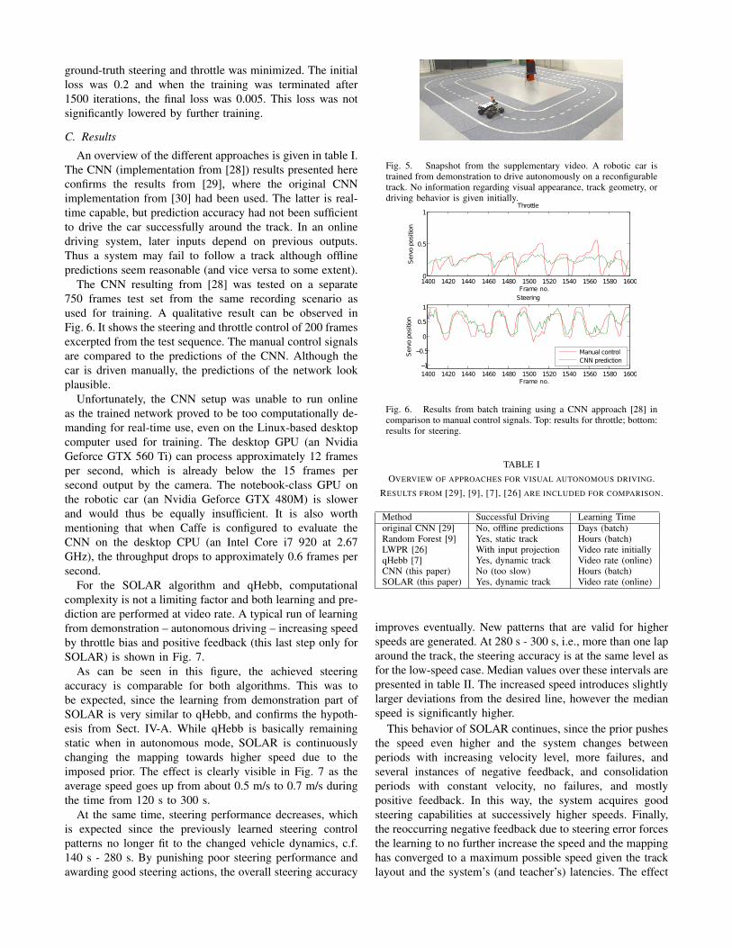
C. Results

An overview of the different approaches is given in table I.The CNN (implementation from [28]) results presented hereconfirms the results from [29], where the original CNNimplementation from [30] had been used. The latter is real-time capable, but prediction accuracy had not been sufficientto drive the car successfully around the track. In an onlinedriving system, later inputs depend on previous outputs.Thus a system may fail to follow a track although offlinepredictions seem reasonable (and vice versa to some extent).

The CNN resulting from [28] was tested on a separate750 frames test set from the same recording scenario asused for training. A qualitative result can be observed inFig. 6. It shows the steering and throttle control of 200 framesexcerpted from the test sequence. The manual control signalsare compared to the predictions of the CNN. Although thecar is driven manually, the predictions of the network lookplausible.

Unfortunately, the CNN setup was unable to run onlineas the trained network proved to be too computationally de-manding for real-time use, even on the Linux-based desktopcomputer used for training. The desktop GPU (an NvidiaGeforce GTX 560 Ti) can process approximately 12 framesper second, which is already below the 15 frames persecond output by the camera. The notebook-class GPU onthe robotic car (an Nvidia Geforce GTX 480M) is slowerand would thus be equally insufficient. It is also worthmentioning that when Caffe is configured to evaluate theCNN on the desktop CPU (an Intel Core i7 920 at 2.67GHz), the throughput drops to approximately 0.6 frames persecond.

For the SOLAR algorithm and qHebb, computationalcomplexity is not a limiting factor and both learning and pre-diction are performed at video rate. A typical run of learningfrom demonstration – autonomous driving – increasing speedby throttle bias and positive feedback (this last step only forSOLAR) is shown in Fig. 7.

As can be seen in this figure, the achieved steeringaccuracy is comparable for both algorithms. This was tobe expected, since the learning from demonstration part ofSOLAR is very similar to qHebb, and confirms the hypoth-esis from Sect. IV-A. While qHebb is basically remainingstatic when in autonomous mode, SOLAR is continuouslychanging the mapping towards higher speed due to theimposed prior. The effect is clearly visible in Fig. 7 as theaverage speed goes up from about 0.5 m/s to 0.7 m/s duringthe time from 120 s to 300 s.

At the same time, steering performance decreases, whichis expected since the previously learned steering controlpatterns no longer fit to the changed vehicle dynamics, c.f.140 s - 280 s. By punishing poor steering performance andawarding good steering actions, the overall steering accuracy

Fig. 5. Snapshot from the supplementary video. A robotic car istrained from demonstration to drive autonomously on a reconfigurabletrack. No information regarding visual appearance, track geometry, ordriving behavior is given initially.

1400 1420 1440 1460 1480 1500 1520 1540 1560 1580 16000

0.5

1Throttle

Ser

vopo

sitio

n

Frame no.

1400 1420 1440 1460 1480 1500 1520 1540 1560 1580 1600−1

−0.5

0

0.5

1

Steering

Ser

vopo

sitio

n

Frame no.

Manual controlCNN prediction

Fig. 6. Results from batch training using a CNN approach [28] incomparison to manual control signals. Top: results for throttle; bottom:results for steering.

TABLE IOVERVIEW OF APPROACHES FOR VISUAL AUTONOMOUS DRIVING.

RESULTS FROM [29], [9], [7], [26] ARE INCLUDED FOR COMPARISON.

Method Successful Driving Learning Timeoriginal CNN [29] No, offline predictions Days (batch)Random Forest [9] Yes, static track Hours (batch)LWPR [26] With input projection Video rate initiallyqHebb [7] Yes, dynamic track Video rate (online)CNN (this paper) No (too slow) Hours (batch)SOLAR (this paper) Yes, dynamic track Video rate (online)

improves eventually. New patterns that are valid for higherspeeds are generated. At 280 s - 300 s, i.e., more than one laparound the track, the steering accuracy is at the same level asfor the low-speed case. Median values over these intervals arepresented in table II. The increased speed introduces slightlylarger deviations from the desired line, however the medianspeed is significantly higher.

This behavior of SOLAR continues, since the prior pushesthe speed even higher and the system changes betweenperiods with increasing velocity level, more failures, andseveral instances of negative feedback, and consolidationperiods with constant velocity, no failures, and mostlypositive feedback. In this way, the system acquires goodsteering capabilities at successively higher speeds. Finally,the reoccurring negative feedback due to steering error forcesthe learning to no further increase the speed and the mappinghas converged to a maximum possible speed given the tracklayout and the system’s (and teacher’s) latencies. The effect

0 50 100 150 200 2500.3

0.4

0.5

0.6

0.7

0.8

Time (s)

Spe

ed (

m/s

)

0 50 100 150 200 250

0

0.2

0.4

0.6

0.8

1

Dis

tanc

e fr

om tr

ack

cent

er (

m)

(a)

0 20 40 60 80 100 120 140 160 180 2000.3

0.4

0.5

0.6

0.7

0.8

Time (s)

Spe

ed (

m/s

)

0 20 40 60 80 100 120 140 160 180 200

0

0.2

0.4

0.6

0.8

1

Dis

tanc

e fr

om tr

ack

cent

er (

m)

(b)

(c)

Fig. 7. Measured deviation from the ideal driving line and speed of the RC-car during (a) SOLAR online learning, (b) qHebb online learning [7] and(c) SOLAR online learning with self-feedback. The line-color at the bottom indicates the driving mode: magenta – learning from demonstration, blue –autonomous driving. The line-color above indicates the reinforcement feedback: green – positive, red – negative, magenta – self-feedback, white – none.See the supplementary video, and section IV-C for an interpretation of these results.

of providing positive or negative feedback to the system isimmediate, thus feedback has to be provided timely, muchlike training a dog.

For providing timely feedback, self-generated feedbackis evaluated, Fig. 7c. After initial training the system isallowed to run four laps autonomously before self-feedbackis activated. This increases the speed of the vehicle. After300 seconds, the system goes beyond its own capabilitiesand manual control is required. After this, speed continuesto increase mostly without supervision. In the end, speed hasincreased more than 0.2 m/s, similar to manual feedback,however less manual supervision was required comparedto feedback learning in (a). Steering deviation decreases(table II), mostly due to additional manual control.

In addition to the experiments performed in a controlled

environment, the system was tested outdoors on gravel andpaved roads. Results are available in the supplementaryvideo. The system is started completely untrained, afteroccasional manual corrections during two minutes in thenight experiment, the vehicle follows the road autonomously.Driving onto a different road type, additional training isprovided during 30 seconds, whereafter the system operatesautonomously.

V. CONCLUSION

We have presented an online learning system based onnon-parametric joint distribution representations where dif-ferent learning modalities are available. This generates ateacher friendly HMI where the teacher may select any typeof learning at any time the teacher finds appropriate. The

TABLE IIMEDIAN SPEED AND DEVIATION FROM THE DESIRED TRAJECTORY,

EVALUATED OVER SELECTED INTERVALS CORRESPONDING TO

DIFFERENT PHASES OF THE EXPERIMENTS.

SOLAR (this paper)Phase Time Speed DeviationInitial training (man.) 0-15s 0.5278 0.0812Auto., after manual (a) 40-110s 0.5249 0.0605Auto., after reinf. 280-300s 0.7415 0.0862Auto., after manual (c) 40-110s 0.3150 0.2347Auto., after self-reinf. 500-600s 0.4331 0.1517Auto., after self-reinf. 1100-1200s 0.5440 0.1427

qHebb [7]Phase Time Speed DeviationInitial training (man.) 0-18s 0.3555 0.1494Auto., after manual (b) 50-200s 0.3630 0.1492Auto., after reinf. Feedback learning not possible.

system, applied to learning autonomous visual road follow-ing, have in experiments demonstrated an ability to learn tofollow roads outdoors, with and without lane markers. Inindoor experiments, the system reached performance levelsbeyond the demonstration of the teacher. Self-generatedfeedback was also sufficient for increasing driving speed, at aslower rate compared to manual feedback. Processing speedis faster than required for video-rate processing both duringtraining and autonomous operation. Driving objectives, e.g.higher driving speed and route selection from higher levelnavigation systems, can be injected using priors.

Thus, learning to drive becomes very similar to humanlearning of the same task. The proposed method workssuperior to several state-of-the-art methods and achieves highaccuracy and robustness in the performed experiments ona reconfigurable track. The ability of associative Hebbianlearning to represent multi-modal mappings is essential e.g.at intersections and in future applications such as obstacleavoidance, where several different actions are appropriate butwhere the average of these actions is not.

ACKNOWLEDGEMENTS

This work has been supported by SSF through the projectCUAS, by VR through VIDI and Vinnova through iQMatic.

REFERENCES

[1] M. F. Land, “Eye movements and the control of actionsin everyday life,” Progress in Retinal and Eye Research,vol. 25, no. 3, pp. 296 – 324, 2006. [Online]. Available:http://www.sciencedirect.com/science/article/pii/S1350946206000036

[2] J. Leonard, J. P. How, S. Teller, M. Berger, S. Campbell, G. Fiore,L. Fletcher, E. Frazzoli, A. Huang, S. Karaman, O. Koch, Y. Kuwata,D. Moore, E. Olson, S. Peters, J. Teo, R. Truax, M. Walter, D. Barrett,A. Epstein, K. Maheloni, K. Moyer, T. Jones, R. Buckley, M. Antone,R. Galejs, S. Krishnamurthy, and J. Williams, The DARPA UrbanChallenge: Autonomous Vehicles in City Traffic. Springer Verlag,2010, vol. 56, ch. A Perception-Driven Autonomous Urban Vehicle.

[3] T. Krajnik, P. Cristoforis, J. Faigl, H. Szuczova, M. Nitsche, M. Mejail,and L. Preucil, “Image features for long-term autonomy,” in ICRAworkshop on Long-Term Autonomy, May 2013.

[4] J. Folkesson and H. Christensen, “Outdoor exploration and slam usinga compressed filter.” in ICRA, 2003, pp. 419–426.

[5] P. Batavia, D. Pomerleau, and C. Thorpe, “Applying advanced learningalgorithms to ALVINN,” Robotics Institute, Pittsburgh, PA, Tech. Rep.CMU-RI-TR-96-31, October 1996.

[6] C. Chen, A. Seff, A. Kornhauser, and J. Xiao, “DeepDriving: Learningaffordance for direct perception in autonomous driving,” in Proceed-ings of the 15th International Conference on Computer Vision, 2015.

[7] K. Ofjall and M. Felsberg, “Biologically inspired online learning ofvisual autonomous driving,” in BMVC, 2014.

[8] A. Oliva and A. Torralba, “Modeling the shape of the scene: aholistic representation of the spatial envelope,” International Journalof Computer Vision, vol. 42, no. 3, pp. 145–175, 2001.

[9] L. Ellis, N. Pugeault, K. Ofjall, J. Hedborg, R. Bowden, and M. Fels-berg, “Autonomous navigation and sign detector learning,” in RobotVision (WORV), 2013 IEEE Workshop on. IEEE, 2013, pp. 144–151.

[10] G. H. Granlund, “An Associative Perception-Action Structure Usinga Localized Space Variant Information Representation,” in Proceed-ings of Algebraic Frames for the Perception-Action Cycle (AFPAC),Germany, September 2000.

[11] M. Felsberg, P.-E. Forssen, and H. Scharr, “Channel smoothing:Efficient robust smoothing of low-level signal features,” IEEE Trans-actions on Pattern Analysis and Machine Intelligence, vol. 28, no. 2,pp. 209–222, 2006.

[12] M. Felsberg, F. Larsson, J. Wiklund, N. Wadstromer, and J. Ahlberg,“Online learning of correspondences between images,” IEEE Trans-actions on Pattern Analysis and Machine Intelligence, 2013.

[13] A. Pouget, P. Dayan, and R. S. Zemel, “Inference and computationwith population codes,” Annu. Rev. Neurosci., vol. 26, pp. 381–410,2003.

[14] R. S. Zemel, P. Dayan, and A. Pouget, “Probabilistic interpretation ofpopulation codes,” Neural Comp., vol. 10, no. 2, pp. 403–430, 1998.

[15] D. W. Scott, “Averaged shifted histograms: Effective nonparametricdensity estimators in several dimensions,” Annals of Statistics, vol. 13,no. 3, pp. 1024–1040, 1985.

[16] M. Felsberg, K. Ofjall, and R. Lenz, “Unbiased decoding of biologi-cally motivated visual feature descriptors,” Frontiers in Robotics andAI, vol. 2, no. 20, 2015.

[17] M. Kass and J. Solomon, “Smoothed local histogram filters,” in ACMSIGGRAPH 2010 papers, ser. SIGGRAPH ’10. New York, NY, USA:ACM, 2010, pp. 100:1–100:10.

[18] L. Sevilla-Lara and E. Learned-Miller, “Distribution fields for track-ing,” in IEEE Computer Vision and Pattern Recognition, 2012.

[19] M. Felsberg, “Enhanced distribution field tracking using channelrepresentations,” in IEEE ICCV workshop on visual object trackingchallenge, 2013.

[20] G. H. Granlund and A. Moe, “Unrestricted recognition of 3-d objectsfor robotics using multi-level triplet invariants,” Artificial IntelligenceMagazine, vol. 25, no. 2, pp. 51–67, 2004.

[21] B. Johansson, “Low level operations and learning in computer vision,”Ph.D. dissertation, Linkoping University, Computer Vision, The Insti-tute of Technology, 2004.

[22] E. Jonsson, “Channel-coded feature maps for computer vision andmachine learning,” Ph.D. dissertation, Linkoping University, Sweden,SE-581 83 Linkoping, Sweden, February 2008, dissertation No. 1160,ISBN 978-91-7393-988-1.

[23] P.-E. Forssen, “Low and medium level vision using channel represen-tations,” Ph.D. dissertation, Linkoping University, Sweden, 2004.

[24] D. Windridge, M. Felsberg, and A. Shaukat, “A framework forhierarchical perception–action learning utilizing fuzzy reasoning,”Cybernetics, IEEE Transactions on, vol. 43, no. 1, pp. 155–169, 2013.

[25] R. P. N. Rao and D. H. Ballard, “Predictive coding in the visualcortex: a functional interpretation of some extra-classical receptive-field effects,” Nature Neuroscience, vol. 2, pp. 79–87, 1999.

[26] K. Ofjall and M. Felsberg, “Online learning of vision-based robotcontrol during autonomous operation,” in New Devel. in Robot Vision,Y. Sun, A. Behal, and C.-K. R. Chung, Eds. Berlin: Springer, 2014.

[27] A. Krizhevsky, I. Sutskever, and G. E. Hinton, “Imagenet classificationwith deep convolutional neural networks,” in Advances in neuralinformation processing systems, 2012, pp. 1097–1105.

[28] Y. Jia, “Caffe: An open source convolutional architecture for fastfeature embedding,” http://caffe.berkeleyvision.org/, 2013.

[29] M. Schmiterlow, “Autonomous path following using convolutionalnetworks,” Master’s thesis, Linkoping University, Computer Vision,The Institute of Technology, 2012.

[30] Y. LeCun, U. Muller, J. Ben, E. Cosatto, and B. Flepp, “Off-roadobstacle avoidance through end-to-end learning,” in Advances inNeural Information Processing Systems (NIPS 2005), Y. Weiss, B.Scholkopf, and J. Platt, Ed., vol. 18. MIT Press, 2005.

Intelligent Vehicles Symposium (IV), 2016 IEEE, 2016, pp. 136-143ISBN: 978-1-5090-1821-5 (online), 978-1-5090-1822-2 (print-on-demand)

DOI: http://dx.doi.org/10.1109/IVS.2016.7535377

Visual Autonomous Road Following by Symbiotic Online Learning

ByKristoffer Öfjäll, Michael Felsberg and

Andreas Robinson

Supplementary files

Channel geometry

The following videos illustrate channel vector curves of N channels. The constant dimension is projected away, leaving a curve in a (N-1)-dimensional space. The curve, together with the (N-1)-simplex rotates in this (N-1)-dimensional space and is orthogonally projected to a 2D space and drawn. Note that the curves are not changing shape, they are only rotating in high dimensional spaces. Four channels, 3D space Five channels, 4D space Seven channels, 6D space

The following videos illustrate the cone (in 3D, and the partially cone-like shape in higher dimensional cases) generated by scaled channel vectors of N channels. The shape is orthogonally projected to a 2D space and drawn. Note that the surfaces are not changing shape, they are only rotating in high dimensional spaces. Three channels, 3D space Four channels, 4D space Seven channels, 7D space

Hebbian Associative Learning

This video illustrates prediction using channel associative learning. During the video, the input value sweeps from 0 to 2 and back to zero. The encoded input value is displayed as scaled basis functions at the bottom of the figure. The elements of the ten by ten linkage matrix C are displayed in the right figure as an image, however since the edge channels have centers outside the representable interval, only the central eight by eight part of C is visible. The left figure shows the corresponding represented joint distribution. The channel encoded output is illustrated as scaled basis functions to the left. In the left figure, the sum of the scaled basis functions is drawn with a dashed line. Associative learning illustration

Non-linear Channel Layouts

The following videos demonstrate logarithmic and log-polar channel arrangements.

Time-logarithmic Channels

Each pixel in one of the PETS-sequences is channel encoded using regularly spaced channels along the intensity axis and logarithmic channel placement along the time dimension. All time values are set to one when encoding. Before encoding and adding a new frame, the time-intensity representation of each pixel is time-shifted using an approximation of the shifting operator which is linear in the channel coefficients. The represented information in five marked pixels is shown as plots where time is along the horizontal axis, with present time to the left, and intensity along the vertical axis, with white at the bottom and black at the top. Decoding of five pixels in a sequence

Log-polar Channel Layout

In the following sequences, each frame is encoded and decoded using spatial channels on a log-polar grid and regularly spaced channels along the intensity. Spatial resolution is thus lower close to the outer edge of the circle. However, intensity resolution is uniform across the image and thus edges of large areas with similar intensity is preserved. Sequence with translating cameraman image Video from UAV and, the original video from the UAV

Autonomous Road Following Application

The first video demonstrates the use case of online learning autonomous road following. The second video shows the capabilities of the demonstrator system. Use case demo Demonstrator system