Embed Size (px)
Citation preview

Visual Impression Localization of Autonomous Robots
Somar Boubou, A.H. Abdul Hafez, Einoshin Suzuki
1. Dept. of Informatics, Kyushu University, Japan.
2. Control Systems Laboratory, Toyota Technological Institute, Japan.
3. Dept. of Computer Engineering, Hasan Kalyoncu University, Turkey.
1
1,2 1 3

Topological visual localization:
• Appearance-based methods:
2
• Landmark-based methods:
[ Pronobis 06]
https://www.dyson360eye.com

Previous Localization methods are precise = every node in the topological map represents a (relatively) precise position of the robot. [Abdul-Hafez13]
Precision: around 1m in outdoor applications, order of mm in indoor applications when geometric features are available. [Badino12][BK Kim15]
3
We achieved a
rough but fast localization with BIRCH.
Background and Objective

Base Work: Autonomous Mobile Robot that Models HSV Color Info. of
the Environment [Suzuki 2012]
Navigating indoor, the robot uses online clustering BIRCH [Zhang 97] and detects peculiar colors
4
X4

Proposed extension to our localization problem
• Robot in [Suzuki12] signals an observation which is sufficiently far from similar past observations
• Our robot inherits most of [Suzuki 12] but solves a localization problem by comparing a pair of CF trees based on All Common Sequence [Wang 97]
5
Observed
data CF tree
on RAM Incremental construction of
the model
Leaf: compressed
similar observations
Outlier (very different from
the corresponding leaf)

Localization problem
Ref1
Nav
Ref4
Ref3
Ref2 Nav CF-tree
Ref CF trees
on ROM
?
Robot localize itself by comparing its tree with several reference trees. Each of which is representing one area of interest.
6

Localization problem
Ref1
Nav
Ref4
Ref3
Ref2 Nav CF-tree
Ref CF trees
on ROM
Robot localize itself by comparing its tree with several reference trees. Each of which is representing one area of interest.
6

Localization problem
Ref1
Nav
Ref4
Ref3
Ref2 Nav CF-tree
Ref CF trees
on ROM
Robot localize itself by comparing its tree with several reference trees. Each of which is representing one area of interest.
6

BIRCH [Zhang 97]
BIRCH, Balanced Iterative Reducing and Clustering using Hierarchies:
• Groups similar examples by building a data index structure called a CF tree (i.e., Clustering Feature tree).
• An efficient and scalable clustering method for a huge data set. [Zhang 97]
Applications:
• Peculiar data discovery [Suzuki 12] and intrusion detection [Horng 11]
7

The Clustering Feature 𝐶𝐹 of a cluster 𝕏 is a triple, denoted as:
CF tree [Zhang 97] 8
N d-dimensional data points or feature vectors x1, x2, … , x𝑁
Cluster 𝕏
𝐿𝑆 = x𝑖𝑁𝑖=1 𝑆𝑆 = x𝑖
2𝑁𝑖=1
𝐶𝐹 = 𝑁, 𝐿𝑆, 𝑆𝑆
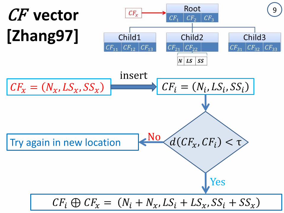
𝑑 𝐶𝐹𝑥 , 𝐶𝐹𝑖 < τ
CF vector [Zhang97]
9
𝐶𝐹𝑖⊕𝐶𝐹𝑥 = 𝑁𝑖 + 𝑁𝑥 , 𝐿𝑆𝑖 + 𝐿𝑆𝑥 , 𝑆𝑆𝑖 + 𝑆𝑆𝑥
𝐶𝐹𝑥 = 𝑁𝑥 , 𝐿𝑆𝑥 , 𝑆𝑆𝑥 𝐶𝐹𝑖 = 𝑁𝑖 , 𝐿𝑆𝑖 , 𝑆𝑆𝑖 insert
Yes
No Try again in new location

CF Vector for HSV color histogram [Suzuki 12]
𝐶𝐹 = 𝑁, 𝐿𝑆, 𝑆𝑆
𝐶𝐹 = (ℎ,𝝎, 𝑛𝑢𝑚, 𝑘𝑒𝑦)
10
𝑘𝑒𝑦 = [𝐵; 𝐺;𝑊; 𝑟0:3; 𝑜0:3; 𝑦0:3; 𝑔0:3; 𝑐0:3; 𝑏0:3; 𝑝0:3]
Our extension: introduction
of weights
[Lei 99]

Robot Navigation
Navigation tree (𝒯)
Paths of tree 1 P
Reference tree (𝒮)
Paths of tree 1 Q
Navigation tree (𝒯)
Comparison of the paths
Arrangement of the comparison results
δ(1,1)= … δ(1,2)= …
.
. δ(P,Q)= …
δ(1)> δ(2)>…> …> δ(P.Q)
S(𝒮,𝒯) = 𝜸 δ(𝒙)𝑷.𝑸𝟏 Similarity(𝒮,𝒯) =
𝑺(𝓢,𝓣)
𝑺(𝓣,𝓣)
𝒮= 𝑆1, 𝑆2, ⋯ , 𝑆𝑃
𝒯= 𝑇1, 𝑇2, ⋯ , 𝑇𝑄
𝛿𝑎𝑐𝑠(𝑝, 𝑞) =𝑎𝑐𝑠 𝑆𝑝, 𝑇𝑞
2𝑀+𝑁ω𝑎𝑐𝑠
𝜸 = 𝑸𝟐/𝑷𝑸 𝑖𝑠 𝑎 𝑠𝑐𝑎𝑙𝑖𝑛𝑔 𝑣𝑎𝑟𝑖𝑎𝑏𝑙𝑒.
Flow Chart for CF-trees comparison

Node weighting
𝛿𝑎𝑐𝑠 =𝑎𝑐𝑠 𝑠, 𝑡
𝑎𝑐𝑠 𝑠, 𝑠 𝑎𝑐𝑠 𝑡, 𝑡𝝎𝒂𝒄𝒔 → 𝛿𝑎𝑐𝑠 =
𝑎𝑐𝑠 𝑠, 𝑡
2𝑀+𝑁𝝎𝒂𝒄𝒔
𝑠 = 𝑆𝑝, 𝑡 = 𝑇𝑞
ω(𝑖) =αω𝑛 + βω𝑝𝑜𝑠
α + β
Let us consider two paths:
12
Weights are used: - to define compression type.
- to eliminate noise.
𝝎𝒂𝒄𝒔 = 1 −max ω𝑠, ω𝑡 −min (ω𝑠, ω𝑡)
max (ω𝑠, ω𝑡)
ω𝑠 = ψω(𝑖)𝑀𝑖=1
[Wang 97]:

Node weighting
𝛿𝑎𝑐𝑠 =𝑎𝑐𝑠 𝑠, 𝑡
𝑎𝑐𝑠 𝑠, 𝑠 𝑎𝑐𝑠 𝑡, 𝑡𝝎𝒂𝒄𝒔 → 𝛿𝑎𝑐𝑠 =
𝑎𝑐𝑠 𝑠, 𝑡
2𝑀+𝑁𝝎𝒂𝒄𝒔
𝑠 = 𝑆𝑝, 𝑡 = 𝑇𝑞
ω(𝑖) =αω𝑛 + βω𝑝𝑜𝑠
α + β
Let us consider two paths:
12
Weights are used: - to define compression type.
- to eliminate noise.
𝝎𝒂𝒄𝒔 = 1 −max ω𝑠, ω𝑡 −min (ω𝑠, ω𝑡)
max (ω𝑠, ω𝑡)
ω𝑠 = ψω(𝑖)𝑀𝑖=1
s={a,b,c} t={a,b} acs(s,t)={∅, 𝑎, 𝑏, 𝑎𝑏}= 4
[Wang 97]:

Node weighting
𝛿𝑎𝑐𝑠 =𝑎𝑐𝑠 𝑠, 𝑡
𝑎𝑐𝑠 𝑠, 𝑠 𝑎𝑐𝑠 𝑡, 𝑡𝝎𝒂𝒄𝒔 → 𝛿𝑎𝑐𝑠 =
𝑎𝑐𝑠 𝑠, 𝑡
2𝑀+𝑁𝝎𝒂𝒄𝒔
𝑠 = 𝑆𝑝, 𝑡 = 𝑇𝑞
ω(𝑖) =αω𝑛 + βω𝑝𝑜𝑠
α + β
Let us consider two paths:
12
Weights are used: - to define compression type.
- to eliminate noise.
𝝎𝒂𝒄𝒔 = 1 −max ω𝑠, ω𝑡 −min (ω𝑠, ω𝑡)
max (ω𝑠, ω𝑡)
ω𝑠 = ψω(𝑖)𝑀𝑖=1
[Wang 97]:
ω𝑛 𝑖 =𝑛𝑖𝑛𝑟𝑜𝑜𝑡
ω𝑝𝑜𝑠 =𝑣
3

Tree types of comparison (favor of root)
𝑘𝑒𝑦 = [𝐵; 𝐺;𝑊; 𝑟0:3; 𝑜0:3; 𝑦0:3; 𝑔0:3; 𝑐0:3; 𝑏0:3; 𝑝0:3]
49_𝑘𝑒𝑦𝑟𝑜𝑜𝑡 = [𝑊: 57%;𝐵: 43%; ]
21_𝑘𝑒𝑦𝑐ℎ𝑖2 = [𝐵: 100%; ]
28_𝑘𝑒𝑦𝑐ℎ𝑖1 = [𝑊: 100%; ]
49_𝑘𝑒𝑦𝑟𝑜𝑜𝑡 = [𝑊: 57%; 𝑟0: 43%; ]
28_𝑘𝑒𝑦𝑐ℎ𝑖1 = [𝑊: 100%; ]
21_𝑘𝑒𝑦𝑐ℎ𝑖2 = [𝑟0: 100%; ]
13

Tree types of comparison (favor of leaves)
𝑘𝑒𝑦 = [𝐵; 𝐺;𝑊; 𝑟0:3; 𝑜0:3; 𝑦0:3; 𝑔0:3; 𝑐0:3; 𝑏0:3; 𝑝0:3]
49_𝑘𝑒𝑦𝑟𝑜𝑜𝑡 = [𝑊: 90%; ]
[𝑟0; 𝑜0; 𝑦0; 𝑔0; 𝑐0; 𝑏0; 𝑝0 = 2% < 5%]
1_𝑘𝑒𝑦𝑐ℎ𝑖2 = [𝐵: 100%; ]
44_𝑘𝑒𝑦𝑐ℎ𝑖1 = [𝑊: 100%; ]
1_𝑘𝑒𝑦𝑐ℎ𝑖3 = [𝐺: 100%; ]
1_𝑘𝑒𝑦𝑐ℎ𝑖6 = [𝑏0: 100%; ]
1_𝑘𝑒𝑦𝑐ℎ𝑖4 = [𝑦0: 100%; ]
1_𝑘𝑒𝑦𝑐ℎ𝑖5 = [𝑐0: 100%; ]
49_𝑘𝑒𝑦𝑟𝑜𝑜𝑡 = [𝑊: 90%; ]
1_𝑘𝑒𝑦𝑐ℎ𝑖2 = [𝐵: 100%; ]
44_𝑘𝑒𝑦𝑐ℎ𝑖1 = [𝑊: 100%; ]
1_𝑘𝑒𝑦𝑐ℎ𝑖3 = [𝐺: 100%; ]
1_𝑘𝑒𝑦𝑐ℎ𝑖6 = [𝑏0: 100%; ]
1_𝑘𝑒𝑦𝑐ℎ𝑖4 = [𝑦0: 100%; ]
1_𝑘𝑒𝑦𝑐ℎ𝑖5 = [𝑐0: 100%; ]
In 𝑘𝑒𝑦𝑟𝑜𝑜𝑡 :
14

Experiments (1)
Favor of the root
Favor of the Leaves
Neutral
- Six areas.
- One reference tree for each area.
- Five navigation trials in each area.
- Three types of comparison were introduced:

Results (1)
Favor of the root Favor of the Leaves Neutral

Experiments (2): KTH-IDOL2 Dataset [ Pronobis06]
- 5 rooms and three illumination conditions which are, cloudy, night, and sunny.
17
Four navigation trials under each condition:
- Three trials were used to create reference CF trees.
-The forth trials were used to create navigation trees.

KTH-IDOL2 Results (2)
0%
20%
40%
60%
80%
Cloudy Night Sunny
Training /Cloudy/
CAMML
NBM
Filter
0%
20%
40%
60%
80%
Cloudy Night Sunny
Training /Night/
0%
20%
40%
60%
80%
Cloudy Night Sunny
Training /Sunny/
[Rubio 14] - /CAMML/ Bayesian Network - Naive Bayes Method

19
- PC with 32-bit Ubuntu 12.04 system.
- Equipped with Intel Core i7 CPU 920.
- Clock speed: 2.67GHz.
- RAM: 11.8GB.
Computation time /Our Platform/

Computation time 20
𝑡𝑎 =29ms
per frame
Paths of tree 1 P
Reference tree (𝒮)
Paths of tree 1 Q
Navigation tree (𝒯)
Compare 𝑇𝑐 = 𝑡𝑐𝑃𝑄
𝑡𝑐 =0.031 ms, P=Q=60 𝑇𝑐 = 111.56 𝑚𝑠
15 fps 𝑄 ≈ 60
𝑇𝑎 = 𝑡𝑎∗ 60 = 435 𝑚𝑠
𝑇𝑡𝑜𝑡 = 𝑡𝑎 + 𝑡𝑐 = 546.56 𝑚𝑠
320×240

Contributions
• We are planning to investigate more robust features (e.g., SIFT, SURF, WI-SURF, HOG) to the changes in the environment due to illumination etc.
21
• Extend the discovery robot [Suzuki 12] for our localization problem.
• Color-based feature were not stable under different illumination conditions.
• Introduce a new measure for CF-tree similarity based on ACS.
Future work

Thank you for listening…