VISIR-I: least-time nautical routes

GMDD8, 7911–7981, 2015

VISIR-I: least-timenautical routes

G. Mannarini et al.

Title Page

Abstract Introduction

Conclusions References

Tables Figures

J I

J I

Back Close

Full Screen / Esc

Printer-friendly Version

Interactive Discussion

Discussion

Paper

|D

iscussionP

aper|

Discussion

Paper

|D

iscussionP

aper|

Geosci. Model Dev. Discuss., 8, 7911–7981, 2015www.geosci-model-dev-discuss.net/8/7911/2015/doi:10.5194/gmdd-8-7911-2015© Author(s) 2015. CC Attribution 3.0 License.

This discussion paper is/has been under review for the journal Geoscientific ModelDevelopment (GMD). Please refer to the corresponding final paper in GMD if available.

VISIR-I: small vessels, least-time nauticalroutes using wave forecasts

G. Mannarini1, N. Pinardi1,2,3, G. Coppini1, P. Oddo2,a, and A. Iafrati4

1Centro Euro–Mediterraneo sui Cambiamenti Climatici – Ocean Predictions and Applications,via Augusto Imperatore 16, 73100 Lecce, Italy2Istituto Nazionale di Geofisica e Vulcanologia, Via Donato Creti 12, 40100 Bologna, Italy3Università degli Studi di Bologna, viale Berti-Pichat, 40126 Bologna, Italy4CNR-INSEAN, Via di Vallerano 139, 00128 Roma, Italyapresently at: NATO Science and Technology Organisation – Centre for Maritime Researchand Experimentation, Viale San Bartolomeo 400, 19126 La Spezia, Italy

Received: 1 August 2015 – Accepted: 14 August 2015 – Published: 11 September 2015

Correspondence to: G. Mannarini ([email protected])

Published by Copernicus Publications on behalf of the European Geosciences Union.

7911

http://www.geosci-model-dev-discuss.net

http://www.geosci-model-dev-discuss.net/8/7911/2015/gmdd-8-7911-2015-print.pdf

http://www.geosci-model-dev-discuss.net/8/7911/2015/gmdd-8-7911-2015-discussion.html

http://creativecommons.org/licenses/by/3.0/

GMDD8, 7911–7981, 2015


G. Mannarini et al.

Title Page



Tables Figures

J I

J I

Back Close

Full Screen / Esc



Discussion

Paper

|D

iscussionP

aper|

Discussion

Paper

|D

iscussionP

aper|

Abstract

A new numerical model for the on-demand computation of optimal ship routes based onsea-state forecasts has been developed. The model, named VISIR (discoVerIng Safeand effIcient Routes) is designed to support decision-makers when planning a marinevoyage.5

The first version of the system, VISIR-I, considers medium and small motor vesselswith lengths of up to a few tens of meters and a displacement hull. The model is madeup of three components: the route optimization algorithm, the mechanical model of theship, and the environmental fields. The optimization algorithm is based on a graph-search method with time-dependent edge weights. The algorithm is also able to com-10

pute a voluntary ship speed reduction. The ship model accounts for calm water andadded wave resistance by making use of just the principal particulars of the vessel asinput parameters. The system also checks the optimal route for parametric roll, pureloss of stability, and surfriding/broaching-to hazard conditions. Significant wave height,wave spectrum peak period, and wave direction forecast fields are employed as an15

input.Examples of VISIR-I routes in the Mediterranean Sea are provided. The optimal route

may be longer in terms of miles sailed and yet it is faster and safer than the geodeticroute between the same departure and arrival locations. Route diversions result fromthe safety constraints and the fact that the algorithm takes into account the full temporal20

evolution and spatial variability of the environmental fields.

1 Introduction

The operational availability of high spatial and temporal resolution forecasts, forboth weather, sea-state and oceanographic variables opens the way to a realm ofdownstream services, which are increasingly closer to end-user needs (Proctor and25

Howarth, 2008). Such services may support the decisional process in critical situations

7912





GMDD8, 7911–7981, 2015


G. Mannarini et al.

Title Page



Tables Figures

J I

J I

Back Close

Full Screen / Esc



Discussion

Paper

|D

iscussionP

aper|

Discussion

Paper

|D

iscussionP

aper|

where knowledge of the present and predicted environmental state is key to avoidingcasualties or to making savings in terms of time, cost, or environmental impact.

VISIR [vi’zi:r]1 is a model and an operational system2 for the on-demand computationof safe and efficient ship routes, based on sea-state forecasts. In its present version,VISIR-I, medium and small motor vessels with displacement hulls are considered, such5

as: fishing vessels (e.g. seiners, trawlers), towboats and fireboats, service boats (crewand supply boats), short trip coastal freighters, displacement hull yachts and pleasurecrafts, and small ferry boats.

The aim of this paper is to lay a sound scientific foundation of VISIR-I, including allits main components: the optimization algorithm, the ship model, and the processing10

of the environmental fields.After reviewing the literature in Sect. 1.1 and summarizing our original contribution

in Sect. 1.2, the solution devised for VISIR-I is presented in detail in Sect. 2. Examplesof optimal routes in the Mediterranean Sea, (Sect. 3), precede the conclusions, whichare drawn in Sect. 4.15

1.1 Review of literature

The main mathematical schemes available in the literature to solve ship routing prob-lems are reviewed in the following.

Initially devised as a manual tool for navigators, the isochrone method is based onthe idea of building an envelope of positions attainable by a vessel at a given time lag20

after departure. This envelope is called an “isochrone”. In the work by Hagiwara (1989),a detailed algorithm is provided, describing how to generate the isochrones and howto use them for constructing a least-time route. Space and course discretization in thevicinity of the rhumb line between departure and arrival locations are performed. At

1“Visir” is the Italian for “vizier”, who was a high-ranking political advisor in the Arab world.Its etymology seems to be related to the ideas of “deciding” and “supporting”.

2http://www.visir-nav.com/

7913





http://www.visir-nav.com/

GMDD8, 7911–7981, 2015


G. Mannarini et al.

Title Page



Tables Figures

J I

J I

Back Close

Full Screen / Esc



Discussion

Paper

|D

iscussionP

aper|

Discussion

Paper

|D

iscussionP

aper|

each progress stage, the course leading to the maximum spatial advancement fromthe origin is considered. When an isochrone gets close enough to the destination, theoptimal route is recovered by a backtracking procedure. No proof of the time-optimalityof the resulting route is provided. Hagiwara’s modified isochrone method is the ba-sis for the fuel optimization method proposed by Klompstra et al. (1992). Here, each5

stage is represented by a two-dimensional position and time. Instead of isochrones ortime-fronts, energy-fronts or “isopones” are computed, being the attainable regions fora given expenditure on fuel. Szlapczynska and Smierzchalski (2007) review severalvariants of the isochrone method, highlighting their weaknesses, such as limitationsin the form of ship speed characteristics and in dealing with landmasses, especially10

in the vicinity of narrow straits. The authors propose a solution to the latter issue, byscreening all route portions intersecting the landmass.

The variational approach involves searching for trajectories making an objective func-tional stationary, such as total time of navigation or operational cost, given a set ofconstraints. The search is achieved by varying the parameters controlling the trajec-15

tory. This approach is equivalent to solving the Euler–Lagrange equation. In Hamilton(1962), least-time ship routes are computed by varying the ship’s course, under the as-sumption that the environmental field is static and thus vessel speed does not explicitlydepend on time.

The time-dependent problem instead can be addressed through the technique of20

optimal control (Pontriagin et al., 1962). With this method, the dynamic system (thevessel) is controlled by a time-dependent input function (typically engine thrust andrudder angle), allowing the objective function to be minimized. Optimal control is for-mulated in terms of a set of necessary conditions (Luenberger, 1979). Applicationsof optimal control to ship routing problems are found in Bijlsma (1975), Perakis and25

Papadakis (1989) and Techy (2011). Least-time transatlantic routes are computed byBijlsma (1975). There, significant wave height and wave direction fields from 12 hourlyforecasts are assumed to determine vessel speed, while the sole control variable isvessel course. The method can account for prohibited courses due to dynamic rea-

7914





GMDD8, 7911–7981, 2015


G. Mannarini et al.

Title Page



Tables Figures

J I

J I

Back Close

Full Screen / Esc



Discussion

Paper

|D

iscussionP

aper|

Discussion

Paper

|D

iscussionP

aper|

sons (e.g. rolling). However, specific geometrical conditions on the vessel speed char-acteristics have to hold for the method to work. Furthermore, due to topological issues,there are unreachable regions of the ocean, and the method involves guessing theinitial vessel course, which may hinder the implementation in an automated system.The approach by Perakis and Papadakis (1989) accounts for a delayed departure time5

and for passage through an intermediate location (point-constrained problem). Localoptimality conditions (“broken extremals”) are found at the boundaries of spatial sub-domains. The optimal ship power setting is found to always take the maximum valuepossible. The results hold under the assumption that the ship speed characteristicsdepend on engine throttle as a multiplicative factor. Another limitation of this approach10

is that the computed extremal trajectory is not guaranteed to lead to a minimum of theobjective function (instead a maximum could be retrieved). In Techy (2011) the authorreports on a vessel moving with constant velocity with respect to water in presenceof currents (“Zermelo’s problem”). The optimal trajectory is analyzed as a function offlow divergence and vorticity, finding the optimal steering policy in a point-symmetric,15

time-varying flow field. In addition, a geometrical interpretation of Pontriagin’s principleis provided. However, to deliver a unique solution, the method requires the hypothesisthat the domain of maneuverability of the ship is convex.

The work by Lolla et al. (2014) is based on the computation of the reachability frontof a vehicle with an internal propulsion system, subject to a time-dependent ocean flow.20

The front is implicitly defined through a level set, and its evolution satisfies a specificsolution of a Hamilton–Jacobi equation. The optimal speed of the vehicle is found toalways take the maximum value admissible. The actual trajectory is computed via back-tracking. This approach allows for both stationary and mobile obstacles, and is able tocompute an optimal departure time for the vehicle. The use of generalized gradients25

and co-states overcome the hypothesis of regularities of the level set. This promisingmethod is at present still lacking an operational implementation.

Monte Carlo methods discard exact solutions in favour of faster solutions. Also, theyprovide a viable technique for fulfilling multiple and competing objectives. A class of

7915





GMDD8, 7911–7981, 2015


G. Mannarini et al.

Title Page



Tables Figures

J I

J I

Back Close

Full Screen / Esc



Discussion

Paper

|D

iscussionP

aper|

Discussion

Paper

|D

iscussionP

aper|

Monte Carlo methods makes use of genetic algorithms. They start with guessed routes(“chromosomes”) whose subparts (“genes”) cross each other and mutate in a randomway, in order to find a new route (“offspring”) that better fits the objective function ofthe actual problem. The use of Monte Carlo methods in the context of multi-objectiveoptimization is reviewed in Konak et al. (2006), while an application to ship routing5

is provided by Szlapczynska (2007). There is also a simulated annealing approach toship routing (Kosmas and Vlachos, 2012). In this case, in order to find a global optimuma trial route is perturbed in a statistical-mechanical fashion. Given that in Monte Carlomethods there is no exact analytical solution, additional criteria are needed in order todecide whether a solution is satisfactory (“convergence test”).10

In discrete methods, the spatial domain is represented by some kind of grid (regu-lar or not) and the optimization is based on recursive schemes. A key concept is theso called principle of optimality: given a point on the optimal trajectory, the remainingtrajectory is optimal for the minimization problem initiated at that point (Luenberger,1979). This property can be stated as a recursive relation, called “Bellman’s condi-15

tion” in the framework of discrete methods. In Zoppoli (1972) a dynamic programmingmethod for the computation of a least-time ship route in the Indian Ocean is used. Thealgorithm is able to ingest time-dependent environmental fields, by evaluating them atthe nearest quantized time value. However, the actual case-study provided in the paperjust uses stationary fields. Ship operating costs for transatlantic routes are minimized20

in Chen (1978), where a terminal cost is also included in the objective function. Thegrid used however is just a band of gridpoints along the rhumb-line track, thus beinglimited in terms of application when there are complex topological constraints, such asin a coastal environment. Takashima et al. (2009) use dynamic programming for com-puting minimum fuel routes of a given duration in time. The propeller revolution number25

is kept constant during the voyage and its value is adjusted in order to reach the targetroute duration. The ship course is varied in order to exploit ocean currents. However,the algorithm uses static environmental information, and re-routing is run every threehours in order to deal with dynamic currents. The dynamic programming method by

7916





GMDD8, 7911–7981, 2015


G. Mannarini et al.

Title Page



Tables Figures

J I

J I

Back Close

Full Screen / Esc



Discussion

Paper

|D

iscussionP

aper|

Discussion

Paper

|D

iscussionP

aper|

Wei and Zou (2012) is used to minimize fuel consumption. Both throttle and headingof the vessel can be optimized, again with grid limitations as in Chen (1978). Montes(2005) employs Dijkstra’s algorithm to compute least-time routes in time-varying fore-cast fields. However, the effect of weather on vessel speed is parametrized in terms ofsubjective parameters (“speed penalty function”).5

1.2 Our contribution

There are several recurrent shortcomings in the ship routing literature: the limited ca-pability to deal with complex topological conditions, such as in the coastal environment(Bijlsma, 1975; Hagiwara, 1989; Szlapczynska and Smierzchalski, 2007); the need forheuristics or subjective parameters in the optimization algorithm (Kosmas and Vlachos,10

2012; Montes, 2005); non explicit use of time-dependent environmental information(Hamilton, 1962; Zoppoli, 1972; Takashima et al., 2009); limitations on the functionaldependence of the vessel response function (Perakis and Papadakis, 1989; Techy,2011); and the not yet demonstrated use in an operational environment (Lolla et al.,2014).15

All these issues need to be addressed simultaneously by a model aimed at feedingan operational system that also works in coastal waters, for a wide class of vesselsand environmental conditions, taking into account navigation safety according to thelatest international standards. In VISIR-I all the above mentioned shortcomings areovercome. The method is based on an exact graph search algorithm, modified in order20

to manage time-dependent environmental fields and voluntary vessel speed reduction.It is validated against analytical results. In addition, the graph grid is designed to dealwith the topological requirements of coastal navigation. VISIR-I also includes a dedi-cated motorboat model and safety constraints for vessel intact stability are considered.

All these features are described in detail in what follows.25

7917





GMDD8, 7911–7981, 2015


G. Mannarini et al.

Title Page



Tables Figures

J I

J I

Back Close

Full Screen / Esc



Discussion

Paper

|D

iscussionP

aper|

Discussion

Paper

|D

iscussionP

aper|

2 VISIR-I method

In this section we present the method employed by VISIR-I for solving the route op-timization problem. First, the problem is formally stated (Sect. 2.1), then the solutionalgorithm (Sect. 2.2), the mechanical model of the ship (Sect. 2.3) and the processingof the environmental analysis and forecast fields affecting the ship dynamics (Sect. 2.4)5

are presented. The structure of the computer code is provided in Sect. 2.5 and a vali-dation of the resulting optimal routes is given in Sect. 2.6.

2.1 Statement of the problem

The mathematical problem addressed and solved in an operational way by VISIR-I canbe stated as follows.10

A ship route is sought departing from A = (xA,tA) and arriving at B = (xB,tA+J) andminimizing the sailing time J defined by

J =1c

B∫A

n(x,t)ds (1)

where x = [x(t), y(t)]T within an open set Ω ⊂R2 denotes horizontal position, t is thetime variable, and15

n(x,t) = c/v(x,t) , (2)

with vessel speed c in calm weather conditions and sustained speed v(x,t) in specificmeteo-marine conditions, is the “refractive index” of a horizontal domain of linear extentds such that

ds2 = dx2 +dy2 (3)20

Note that the integrand in Eq. (1) can be interpreted as an effective optical depth ofthe ds wide domain. The notation is reminiscent of the problem of determining the path

7918





GMDD8, 7911–7981, 2015


G. Mannarini et al.

Title Page



Tables Figures

J I

J I

Back Close

Full Screen / Esc



Discussion

Paper

|D

iscussionP

aper|

Discussion

Paper

|D

iscussionP

aper|

of light moving in a non homogenous medium. Indeed light propagates over paths ofstationary optical depth (Fermat’s principle).

Ship speed v results from a dynamic balance between forces and torques actingon and from the vessel. This speed is normally found as the solution of differentialequations. However, under steady conditions they reduce to algebraic equations of the5

type:

Feq(v ;ps,pe) = 0 (4)

where ps is a set of ship parameters and pe a set of values of relevant environmentalfields evaluated at (x,t). Navigational safety also poses limitations on the admissiblesolutions of Eq. (4). Such limitations are represented as a set of inequalities of the type:10

Fineq(v ;ps,pe) ≤ 0 (5)

Parameters ps and pe employed in Eqs. (4) and (5) are listed in Table 6.If the open set Ω is also a connected domain, the existence of a solution to the

problem Eqs. (1)–(5) entirely depends on Eqs. (4) and (5): The quality of the route, itstopological and nautical characteristics, are determined by these two equations alone.15

Speed v resulting from Eqs. (4) and (5) defines the Lagrangian kinematics of theroute:

dsdt

= v(x,t) (6)

In order to account for uncertainty in the representation of v , a random noise term couldbe added to the r.h.s. of Eq. (6).20

The problem of finding the least-time route in any meteo-marine conditions is thusequivalent to the minimization of J functional with a specified refractive index n(x,t),for assigned boundary values A and B.

If the time-dependence in refractive index n is neglected, the general solution of thisproblem is known from geometrical optics, with routes being refracted towards optically25

7919





GMDD8, 7911–7981, 2015


G. Mannarini et al.

Title Page



Tables Figures

J I

J I

Back Close

Full Screen / Esc



Discussion

Paper

|D

iscussionP

aper|

Discussion

Paper

|D

iscussionP

aper|

more transparent regions, according to Snell’s law. However, whenever the time scalefor changes in the environmental fields is comparable or shorter than the typical routeduration, such time-dependence can no longer be neglected and new kinematical fea-tures of the least-time route may appear. Indeed, it could be advantageous to wait forsome time at the departure location before leaving or voluntarily decrease the speed5

during navigation, as shown in Sect. 2.2.2 and 2.2.3.

2.2 Shortest path algorithm

The first component of VISIR-I presented here is the shortest path algorithm. The term“shortest path” is used both in the literature and hereafter with a more general sensethan a direct reference to the geometrical distance. Indeed, “shortest” may refer to the10

spatial or temporal distance, as well as the cost or other figure of merit of the optimalpath.

2.2.1 Spatial discretization

Let us consider a directed graph G = [N , E]. In VISIR-I the nodes N are part of a rect-angular mesh with constant spacing in natural coordinates (1/60 of resolution in both15

latitude and longitude). As shown in Fig. 1, each node is linked to all its first and secondneighbours on the grid, forming the set of edges E. Thus, neglecting border effects,there are 24 connections per node. The specific edge arrangement leads to resolveangles of

θ12 = arctan(1/2) ≈ 26.6 (7)20

Whether such such 24-connectivity should be increased further is questionable, giventhat the environmental analysis and forecast fields are provided on a coarser grid (byabout a factor of 4) than the spatial resolution of the graph, see Sect. 2.4.

In VISIR-I, the resulting graph is first screened for nodes and edges on the landmass.An edge is considered to be on the landmass if at least one of its nodes is on the25

7920





GMDD8, 7911–7981, 2015


G. Mannarini et al.

Title Page



Tables Figures

J I

J I

Back Close

Full Screen / Esc



Discussion

Paper

|D

iscussionP

aper|

Discussion

Paper

|D

iscussionP

aper|

landmass or if both nodes are in the sea and the edge linking them intersects thecoastline. In such a case, the edge is removed from E, which locally reduces the original24-connectivity of the graph. When applied to a 1/60 grid for the Mediterranean Searegion (mode 1 of Fig. 8), this procedure still leaves more than 20 million sea edges inE, see Table 2. However, for the actual route computations, just a subset of the whole5

spatial domain is considered (mode 2 of Fig. 8). This subregion is chosen to be largeenough so that a further increase in size does not reduce the total sailing time J . Atpresent, the selection of the subregion shape and extent is left to the user of the model.

2.2.2 Time-dependent approach

Given that environmental conditions change over a time scale comparable with or10

shorter than the vessel route duration, edge weights cannot be considered as con-stants. Thus, in order to solve Eqs. (1)–(3), VISIR-I employs a time-dependent algo-rithm.

With reference to the nomenclature in Table 1, a time-dependent graph G(t) isfully defined by the sets of nodes, edges, and time-dependent edge weights: G(t) =15

[N , E,A(t)].Edge weight ajk(`) between nodes j and k at time step ` is defined as

ajk(`) =|xk −xj |vjk(`)

(8)

where vjk(`) is the edge mean ship speed, depending on the average Φjk of the valuesof the environmental fields at nodes j and k:20

Φjk =12

(Φj +Φk

)(9)

evaluated at time t` = t1 +δt(` −1). Here t1 is departure time and δt is the time reso-lution of the environmental fields. The functional dependence of vjk(`) on Φjk resultsfrom the actual model of the vessel, and is derived in Sect. 2.3.

7921





GMDD8, 7911–7981, 2015


G. Mannarini et al.

Title Page



Tables Figures

J I

J I

Back Close

Full Screen / Esc



Discussion

Paper

|D

iscussionP

aper|

Discussion

Paper

|D

iscussionP

aper|

Thus, in VISIR-I, edge weights ajk(`) are non-negative quantities with a dimensionof time (“edge delays”) and are time-dependent. Note that Eq. (8) is the discrete coun-terpart of Eq. (6), as long as velocity is non null.

There are various methods for computing shortest paths on a graph. For an overview,see Bertsekas (1998) and Bast et al. (2014). A large literature deals with applications5

for terrestrial networks, see e.g. Zhan and Noon (1998); Zeng and Church (2009);Goldberg and Harrelson (2005).

A key concept in graph methods is the node label, which can be either temporary orpermanent. The permanent label Xj of node j is the minimum value of the objectivefunction (e.g. J of Eq. 1) attainable at that node. A temporary label Yj is any value10

before the node label is set to its permanent value. When all node labels are set totheir permanent value, Bellman’s relation holds (Bertsekas, 1998).

Depending on the way node labels are updated, graph algorithms may be classifiedinto label setting or label correcting algorithms. A label setting single-source single-destination algorithm with fixed departure time is used here.15

The fact that in VISIR-I destination node is assigned (through xB in Eq. 1) leadsto a possible degeneracy of the problem, with multiple shortest paths between thespecified source and destination node. In Yen (1971) an algorithm is presented forfinding several simple shortest paths. In VISIR-I it is deemed that, in presence of time-dependent environmental fields, it is unlikely that an alternative route with exactly the20

same navigation time exists. Thus, just the least-time route is sought after.In general, the fact that a graph is time-dependent means that the shortest path can

have special features. In fact, under specific circumstances, the strategy of traversingan edge as soon as possible does not always lead to the shortest path. Also, the short-est path may not be simple (there may be loops) or even not concatenated (Bellman’s25

optimality not fulfilled). This has consequences on the class of algorithm to be applied.Orda and Rom (1990) show that in this respect the critical condition is how fast edgedelays vary in time. If ajk(t) is a differentiable function of time t, the authors show that,

7922





GMDD8, 7911–7981, 2015


G. Mannarini et al.

Title Page



Tables Figures

J I

J I

Back Close

Full Screen / Esc



Discussion

Paper

|D

iscussionP

aper|

Discussion

Paper

|D

iscussionP

aper|

provided

ddtajk(t) ≥ −1, (10)

the best strategy for recovering a shortest path is traversing edge (jk) without waitingat node j (First-In First-Out or: FIFO). Indeed, waiting for a time dt > 0 would in bestcase be compensated but never overcome by a related decrease |dajk | ≤ dt in edge5

delay. The authors also show that a FIFO time-dependent algorithm has the samecomputational complexity as a static algorithm.

Typically, condition Eq. (10) may be violated during the decaying phase of a rapidlymoving storm. Since VISIR-I employs sea state fields for the Mediterranean Sea, thevariability of edge delays is usually low, so that condition Eq. (10) is generally fulfilled,10

as seen from Fig. 2. The FIFO condition Eq. (10) is also checked at each run of themodel and is generally found to be fulfilled. Thus, Dijkstra’s static algorithm (Dijkstra,1959) is modified according to the guidelines of Orda and Rom’s FIFO time-dependentalgorithm. Related pseudocode is provided in Appendix A.

Before the algorithm is run, edge delays ajk(`) are checked for nautical safety15

constraints, Eq. (5). If at time step ` an edge (j k) is unsafe for navigation, we setaj k(`) =∞. As seen from Fig. 2, this approach generates gaps in aj k(t) as a functionof continuous time t. Such gaps are specific time windows during which the edge isnot available for linking its nodes. Whenever edges are removed at specific time steps,a FIFO strategy is no longer guaranteed to be optimal, even though edge delays vary20

slowly. A source-waiting strategy may be necessary in this case (Orda and Rom, 1990).As a consequence, a route retrieved through a FIFO algorithm may still be sub-optimal.This advanced issue is left open for future versions of the system.

2.2.3 Voluntary speed reduction

As seen above, VISIR-I’s strategy regarding navigational safety is to remove unsafe25

edge delays from the graph by setting their edge weight to∞, prior to the computation7923





GMDD8, 7911–7981, 2015


G. Mannarini et al.

Title Page



Tables Figures

J I

J I

Back Close

Full Screen / Esc



Discussion

Paper

|D

iscussionP

aper|

Discussion

Paper

|D

iscussionP

aper|

of the optimal route. In addition, as will be shown in Sect. 2.3.3, vessel speed v affectsthe safety constraints. Thus, a modification of v may help in keeping an otherwise un-safe edge in the graph. This, in turn, may contribute to optimization, since avoiding theremoval of elements from set A(t) can only lower the length of the shortest path. Suchvoluntary variations in speed should be contrasted with an involuntary speed reduc-5

tion due to vessel energy loss, caused by interaction with the environmental fields, seeSect. 2.3.2.

VISIR-I defines, for a vessel with maximum engine power Pmax, a set of possiblevalues P (s)/Pmax of engine throttle:

P (s) = Pmax ·g(s) (11)10

s ∈ [1,Ns]

Then, at each edge, speeds v (s)jk (`) are computed using the ship model. The function

g(s) is chosen in order to linearly space engine throttle values, Table 3 (due to thenon-linearity of the vessel model, this choice does not imply linearly spaced values ofsustained speed, see Fig. 5). Next, throttle-dependent edge weights a(s)

jk (`) are com-15

puted via Eq. (8). Each of these edge weights is checked to see whether it complieswith navigational safety constraints. If an edge is unsafe, its edge weight is set to ∞.Finally, the throttle value s∗ leading to the minimum edge weight is chosen by the algo-rithm:

s∗ = argmins

a(s)jk (`)

(12)20

and the edge weight is set to such a minimum value:

ajk(`) = a(s∗)jk (`) (13)

Given the ordering in Table 3, if s∗ > 1 then voluntary speed reduction is useful forrecovering a faster route which is still safe with respect to ship stability constraints.

7924





GMDD8, 7911–7981, 2015


G. Mannarini et al.

Title Page



Tables Figures

J I

J I

Back Close

Full Screen / Esc



Discussion

Paper

|D

iscussionP

aper|

Discussion

Paper

|D

iscussionP

aper|

2.3 Ship model

The second component of VISIR-I is a ship model describing vessel interaction with theenvironment (specified by the forecast fields of Sect. 2.4) and its stability requirements.

The following presentation comprises a balance equation for the propulsion sys-tem Sect. 2.3.1, a parametrization of the hull resistance due to calm and rough sea5

Sect. 2.3.2, and a set of dynamic conditions for the intact stability of the vesselSect. 2.3.3.

2.3.1 Propulsion

Motorboats are the focus of VISIR-I route optimization.For these vessels, propulsion is provided by a thermal engine burning fuel and deliv-10

ering a torque to the shaft line and, when present, to a gearbox. This torque is eventu-ally transmitted to a propeller, converting it into thrust available to counteract resistanceto advancement (Journée, 1976; Triantafyllou and Hover, 2003).

A full modelling of this energy conversion mechanism is a highly complex task involv-ing, just to mention a few, the efficiency of each of these conversion steps, the effect15

of hull-generated wake on propeller efficiency and corresponding thrust deduction, andthe load conditions of the engine (MANDieselTurbo, 2011). A quantitative description ofthese processes requires a detailed knowledge of engine and vessel behaviour. Thiscould be obtained by standard measurement procedures such as those provided bythe International Towing Tank Conference (ITTC, 2002, 2011b).20

For the purposes of VISIR-I, it was deemed sufficient to derive the vessel responsefunction from a power balance. That is, given the brake power P , the total propulsiveefficiency η and the total resistance RT applied to the vessel, it is required that

ηP = −v ·RT(v) (14)

where v is ship velocity in steady conditions. The l.h.s. of Eq. (14) represents the power25

available at the propeller, while resistance RT(v) depends on both environmental and7925





GMDD8, 7911–7981, 2015


G. Mannarini et al.

Title Page



Tables Figures

J I

J I

Back Close

Full Screen / Esc



Discussion

Paper

|D

iscussionP

aper|

Discussion

Paper

|D

iscussionP

aper|

ship parameters. One of its possible representations is derived in Sect. 2.3.2. Theefficiency η results from the product of several components related, for example, to hullshape, propeller, and shaft characteristics (MANDieselTurbo, 2011). At the presentstage of modelling, the value of η is estimated to a constant (see Table 4) and will berefined when a more detailed vessel model is used.5

2.3.2 Resistance

In this paper we restrict our attention to displacement vessels. Indeed high speed plan-ing hulls are characterized by a different dynamic behaviour and deserve a more so-phisticated treatment (Savitsky and Brown, 1976).

When underway, a displacement vessel is subject to various forces hindering its10

motion. A possible decomposition of the resulting force is to distinguish calm waterresistance Rc from resistance Raw due to only sea waves,

RT = Rc +Raw (15)

Since calm water resistance is always opposite to the ship direction of advance, de-composition Eq. (15) enables Eq. (14) to be rewritten as15

ηP = v (Rc +Raw cosα) (16)

where α is the angle between wave direction and vessel direction of advance (as seenfrom Fig. 3, α = 0 in case of head waves).

The module of the calm water resistance is usually given in terms of a dimensionlessdrag coefficient CT defined by the equation20

Rc(v) = CT12ρSv2 (17)

where also sea water density ρ and ship wetted surface S appear.

7926





GMDD8, 7911–7981, 2015


G. Mannarini et al.

Title Page



Tables Figures

J I

J I

Back Close

Full Screen / Esc



Discussion

Paper

|D

iscussionP

aper|

Discussion

Paper

|D

iscussionP

aper|

As outlined in ITTC (2011a), CT depends not just on viscous effects but also on en-ergy dissipated in gravity waves generated by the vessel (“residual resistance”). Thelatter introduces a dependence on Froude Number Fr which, under Froude’s hypoth-esis, is additive: CT(R,F r) ≈ CF(R)+CR(F r), where R is Reynold’s number and CR isthe residual resistance drag coefficient (Newman, 1977).5

In VISIR-I, at this first stage in the development of the ship model, CT is taken asa constant. This is done in order to easily identify the unknown coefficients in the r.h.s.of Eq. (17). Indeed, the CTS product is obtained by equating the maximum availablepower at the propeller to the power dissipation occurring at top speed c in calm water:

ηPmax = c ·Rc(v = c) = CT12ρSc3 (18)10

The impact of assuming a constant CT is to overestimate it at low speeds, as thiscoefficient is identified using the top speed regime, Eq. (18).

In addition to calm water resistance, sea waves are an additional source of ship en-ergy losses (Lloyd, 1998). Various authors have found that wave-added resistance Rawdepends on reduced wavenumber L/λ, where L is ship length. Both radiation (energy15

dissipated due to heave and pitch movements) and diffraction (energy dissipated bythe hull to deflect short incoming waves) contribute to this additional resistance. Botheffects were modeled by Gerritsma and Beukelman (1972) in head seas, which how-ever are the most severe conditions in terms of added resistance. They found thatdiffraction increases resistance at L/λ > 1. In the framework of a comprehensive study20

of experimental results and several different theoretical methods, Ström-Tejsen et al.(1973) endorsed the method by Gerritsma and Beukelman (1972).

In VISIR-I, a simplified approach for estimating Raw is used. Following the cited liter-ature, a reduced non-dimensional resistance σaw is introduced:

Raw = σaw(L,B,T ,F r) ·ρg0ζ

2B2

L·ϕ(λL

,α)

(19)25

7927





GMDD8, 7911–7981, 2015


G. Mannarini et al.

Title Page



Tables Figures

J I

J I

Back Close

Full Screen / Esc



Discussion

Paper

|D

iscussionP

aper|

Discussion

Paper

|D

iscussionP

aper|

The relation between wave amplitude and significant wave height is 2ζ = Hs. In Eq. (19)a factor ϕ is highlighted, containing the spectral and angular dependencies. This factoris eventually set to a constant value ϕ0. This approximation is also done in view ofthe fact that the full wave spectrum is not used for weighting Raw, as instead done, forexample, in Ström-Tejsen et al. (1973). In line with dropping the α dependence in ϕ,5

the vectorial nature of Raw, Eq. (16), is ignored by assuming that this force is alwaysopposite to the ship’s forward speed in a longitudinal direction (α = 0).

A simplified method for deriving σaw when the hull geometry is not available in itsentirety was proposed by Alexandersson (2009). We slightly modified his results into:

σaw = σaw F r/F r (20)10

σaw = 20. (B/L)−1.20(T/L)0.62 (21)

Further details of this derivation can be found in Appendix B.Combining Eqs. (20)–(21) with Eq. (19) shows that an increase in either ship beam or

draught leads to an increase in resistance, while an increase in length has the oppositeeffect. This conclusion should be validated through towing tank measurements on the15

specific hull geometry.Replacing Eqs. (15)–(21) into Eq. (14) where α = 0, the following expression is found

to relate ship speed to brake power, geometrical vessel parameters, and environmentalfields:

k3v3 +k2v

2 − P = 0 (22)20

where the coefficients are given by

k3 =Pmax

c3(23)

k2 = σaw1

ηF rϕ0ρζ

2B2√g0/L3 (24)

7928





GMDD8, 7911–7981, 2015


G. Mannarini et al.

Title Page



Tables Figures

J I

J I

Back Close

Full Screen / Esc



Discussion

Paper

|D

iscussionP

aper|

Discussion

Paper

|D

iscussionP

aper|

Note that Eq. (22) is in the form of Eq. (4) with parameters ps and pe as in Table 6.Sustained speed v is the sole positive root of cubic equation Eq. (22) (in fact, both

k3 and k2 coefficients are positive quantities). This is computed through an analyti-cal expression whose numerical implementation is provided by Flannery et al. (1992,Sect. 5.6). In Fig. 4 corresponding sustained Froude numbers Fr are displayed. Fr fol-5

lows a half-bell shaped curve, with a nearly hyperbolical (∼ 1/Hs) dependence for largesignificant wave height. However, in the results shown by Bowditch (2002, Fig. 3703)for a commercial 18-knot vessel, a change of convexity of the Fr curve is not visible, forthe Hs range shown. Our results also prove that, by varying engine throttle, sustainedspeed does not vary by the same factor at all Hs. This result could not be obtained10

by factorizing the throttle dependence, as in the ship model by Perakis and Papadakis(1989). Furthermore, by comparing performances of vessel V1 (ferryboat) and V2 (fish-ing vessel) in Fig. 4, it can be seen that the former sustains a larger fraction of its topFroude number at any given significant wave height. This different dynamic behaviouris mainly related to the maximum engine brake power Pmax of the two vessels. This15

is found by swapping just Pmax of the two vessels and keeping unchanged the otherparameters provided in Table 5 (not shown).

Figure 5 shows how the throttle needs to be adjusted to sustain a given speed indifferent sea states. An increase in speed requires an over-proportional increase inthrottle. This leads, for each given sea state, to a so called “wave wall” (MANDiesel-20

Turbo, 2011). Lloyd (1998) makes the assumption that the engine delivers constantpower at a given throttle setting, regardless of the increased propeller load due to roughweather (note that propeller load is not considered in VISIR-I either). He then finds thatthe power required for sustaining a given speed steeply rises with wave height, similarto Fig. 5. The comparison between V1 and V2 also shows that the two vessels behave25

very differently in extreme seas, whereby vessel V1 (the ferryboat) is able to reachmore than 30 % while V2 (the fishing vessel) less than 20 % of its top Fr. Again it isimportant to note that these results were obtained under the hypothesis of neglectingthe residual resistance in CT.

7929





GMDD8, 7911–7981, 2015


G. Mannarini et al.

Title Page



Tables Figures

J I

J I

Back Close

Full Screen / Esc



Discussion

Paper

|D

iscussionP

aper|

Discussion

Paper

|D

iscussionP

aper|

Resistances are evaluated from the sustained speed v as:

Rc = ηk3v2 (25)

Raw = ηk2v (26)

and corresponding values are shown in Fig. 6.While calm water resistance Rc does not explicitely depend on significant wave5

height Hs, Rc depends on ship speed which, through Eqs. (22)–(24), depends on Hs.Thus, assuming maximum throttle, a functional dependence Rc = Rc(Hs) can be com-puted and is displayed in Fig. 6. Due to the fact that k3 is independent of Hs (Eq. 23),calm water resistance Rc is dominated by the v = v(Hs) relationship seen in Fig. 4.

Wave added resistance Raw as a function of Hs initially grows quadratically and, for10

higher waves, only linearly, Fig. 6. This is due to the combined effect of the quadraticdependence on wave amplitude in k2 (Eq. 24) and the nearly hyperbolic ship speedreduction for large Hs seen in Fig. 4. The same trend is observed in (Lloyd, 1998,Fig. 3.13) and Nabergoj and Prpić-Oršić (2007).

In comparison to V2, vessel V1 exhibits larger resistances. However, for both vessel15

classes, the Rc and Raw curves form “scissors”, being wider for the larger vessel (V1),Fig. 6.

2.3.3 Stability

The ship model described so far needs to be complemented by navigational constraintsin order to reduce dangerous or unpleasant movements for the ship itself, the crew and20

cargo.Such situations cannot simply be ruled out by designing a vessel in accordance

with the Intact Stability (IS) Code, IMO (2008). In fact, specific combinations of mete-orological and sea-state parameters may lead to dangerous situations even for shipscomplying with such mandatory regulations (Umeda, 1999; IMO, 2007). Furthermore,25

in Belenky et al. (2011) the point is made that new ship forms can make the prescription

7930





GMDD8, 7911–7981, 2015


G. Mannarini et al.

Title Page



Tables Figures

J I

J I

Back Close

Full Screen / Esc



Discussion

Paper

|D

iscussionP

aper|

Discussion

Paper

|D

iscussionP

aper|

of the IS code obsolete. This led to the development of “second generation” stabilitycriteria, being more physics and less statistics based than IS criteria.

VISIR-I checks for three modes of stability failure: parametric roll, pure loss of sta-bility, and surfriding/broaching-to. The theoretical hints below are mainly based on Be-lenky et al. (2011), while the implementation of the stability checks follows the op-5

erational guidance by IMO more closely (IMO, 2007). In view of the limited angularresolution of the graph (Sect. 2.2.1), in VISIR-I stability in turning (Biran and Pulido,2013) cannot be taken into consideration, and an unlimited vessel manoeuvrability(IMO, 2002) has to be assumed.

A realistic assessment of stability failure would require a detailed knowledge of ship10

hull geometry. In the present version of VISIR-I, however, just principal particulars ofthe vessel (length, beam, draught) are employed. In addition, even vessel-internal mo-tions and mass displacements, such as the positioning of catch (Gudmundsson, 2009)and fuel sloshing (Richardson et al., 2005) may have an amplifying effect on the lossof stability. Thus, the bare application of safety constraints described in the following15

cannot guarantee navigation safety, and the ship-master should critically evaluate theresulting route computed by VISIR-I, also taking account the meteo-marine conditionsactually met during the voyage and the specific vessel response.

In the following sections, we have used the deep water approximation in order to gaina rapid estimation of the threshold conditions. We can thus estimate the wavelength as:20

λ[m] =g0

2πT 2

w ≈ 1.56(Tw[s])2 (27)

and the wave phase speed or celerity as:

cp[kt] =

√g0λ2π≈ 2.4

√λ[m] ≈ 3Tw[s] (28)

7931





GMDD8, 7911–7981, 2015


G. Mannarini et al.

Title Page



Tables Figures

J I

J I

Back Close

Full Screen / Esc



Discussion

Paper

|D

iscussionP

aper|

Discussion

Paper

|D

iscussionP

aper|

Then, assuming a fully developed sea (Pierson–Moskowitz spectrum), the wave steep-ness can be estimated as:

Hs/λ =2πg0

Hs

T 2w

=8π

(24.17)2≈ 1/23 (29)

This result can be inferred from the plot of characteristic seas reported by Ström-Tejsenet al. (1973). For partially developed seas the wave steepness is larger and for dying5

seas smaller than the value obtained in Eq. (29).

2.3.4 Parametric roll

When a ship is sailing in waves, the submerged part of the hull changes in time. Formost hull shapes, this also involves a change in the waterplane area. This in turninfluences the curve for the righting lever (GZ), which is fundamental to ship stability.10

Indeed, if wavelength λ is comparable to ship length L and waves are met at a specificfrequency, the change in GZ may trigger a resonance mechanism, leading to a dramaticamplification of roll motion (Belenky et al., 2011). A famous naval casualty ascribed tothis mechanism of stability loss is reported in France et al. (2003).

The mathematical formulation of parametric roll is based on the solution of Mathieu’s15

equations and the computation of Ince–Strutt’s diagram. It shows that parametric rolloccurs when encounter wave period TE satisfies the condition

2TE = ±nTR,n = 1,2,3, . . . (30)

where TR is the ship’s natural roll period (Spyrou, 2005) and the ± sign in Eq. (30)accounts for both following and head seas.20

In VISIR-I the encounter period TE is obtained by applying a Doppler’s shift to peakwave period Tw and reads

TE = Tw ·[

1+v cosα

3TwK (Tw,z)

]−1

(31)

7932





GMDD8, 7911–7981, 2015


G. Mannarini et al.

Title Page



Tables Figures

J I

J I

Back Close

Full Screen / Esc



Discussion

Paper

|D

iscussionP

aper|

Discussion

Paper

|D

iscussionP

aper|

where Fenton’s factor K defined by Eq. (48) is used (v in kt). Instead, IMO’s formula forTE provided in (IMO, 2007, 1.6) corresponds to the deep water approximation, i.e. tothe case K = 1. Since in shallow waters and large wave periods K < 1, IMO’s formulamay lead to an overestimation of TE.

Levadou and Gaillarde (2003) observe that a smaller GM also implies a larger natural5

roll period TR and thus a parametric roll experienced in presence of longer waves.Spyrou (2005) points out that, while any encounter angle α can in principle lead toparametric roll, vessels with low metacentric height GM (and, thus, large TR) may bemore prone to experience parametric roll during following than head seas (due to larger|TE|).10

Following (Levadou and Gaillarde, 2003) and the wave height criterion reported forL < 100 m in Belenky et al. (2011), the parametric roll hazard condition is implementedin VISIR-I as:

0.8 ≤ λ/L ≤ 2 (32)

Hs/L ≥ 1/20 (33)15

together with Eq. (30) expressed in the form of the inequalities:

1.8|TE| ≤ TR ≤ 2.1|TE| (34)

0.8|TE| ≤ TR ≤ 1.1|TE| (35)

where the coefficients in Eqs. (34)–(35) should be related to the roll damping charac-teristics of the vessel (Francescutto and Contento, 1999), but for the current version of20

VISIR-I they are taken from Benedict et al. (2006).Formula Eq. (31) shows that TE period may be tuned by varying the speed and course

of the vessel. Thus, to prevent parametric rolling, a routing algorithm may suggest eithera voluntary speed reduction or a route diversion. As shown in Sect. 2.2.3 and as willbe seen in the case studies (Sect. 3), VISIR-I is able to exploit either option.25

7933





GMDD8, 7911–7981, 2015


G. Mannarini et al.

Title Page



Tables Figures

J I

J I

Back Close

Full Screen / Esc



Discussion

Paper

|D

iscussionP

aper|

Discussion

Paper

|D

iscussionP

aper|

2.3.5 Pure loss of stability

This mode of stability failure is triggered by a similar condition to the parametric roll.However, it does not involve any resonance mechanism and thus may be activated bya single wave. In fact, if the crest of a large wave is near the midship section of theship, stability may be significantly decreased. If this condition lasts long enough (such5

as during following waves and ship speed close to wave celerity), the ship may developa large heel angle, or even capsize.

According to Belenky et al. (2011) a useful criterion for distinguishing ships proneto pure loss of stability involves a detailed knowledge of hull geometry. The IMO guid-ance (IMO, 2007) however proposes using just ship-wave kinematics. This is also the10

criterion adopted in VISIR-I and can be stated as the following conditions to be simul-taneously verified:

λ/L ≥ 0.8 (36)

Hs/L ≥ 1/25 (37)

|π−α| ≤ π/4 (38)15

1.3Tw ≤ v · cos(π−α) ≤ 2.0Tw (39)

where ship speed v is given in kt.Using also Eqs. (27)–(28) it can be seen that Eq. (39) implies (for exactly following

seas) a sustained speed v between 43 and 67 % of wave celerity cp.

2.3.6 Surfriding/broaching-to20

Surfriding is the condition where the wave profile does not vary relative to the ship.That is, the ship moves with a speed equal to wave celerity: v = cp. In this case, theship is directionally unstable, with the possibility of an uncontrollable turn known as“broaching-to”.

7934





GMDD8, 7911–7981, 2015


G. Mannarini et al.

Title Page



Tables Figures

J I

J I

Back Close

Full Screen / Esc



Discussion

Paper

|D

iscussionP

aper|

Discussion

Paper

|D

iscussionP

aper|

The simplest modelling of this mode of stability failure starts with the computation ofthe force of the wave-induced surge which is able to balance the difference betweentotal resistance and thrust provided by the ship. A critical point may then be reached,where surging is no longer possible and the ship is captured by the surfriding mode(Belenky et al., 2011). This phase transition is a heteroclinic bifurcation (Umeda, 1999).5

In IMO (2007) a surfriding condition is proposed which just takes into account shipspeed and length, independently of wave steepness. Based on numerical simulations,Belenky et al. (2011) overcomes this simplification, with the finding that the phasetransition is less likely for less steep waves.

In VISIR-I, the following surfriding hazard criteria reported in Belenky et al. (2011)10

are considered:

0.8 ≤ λ/L ≤ 2 (40)

Hs/λ ≥ 1/40 (41)

|π−α| ≤ π/4 (42)

F r · cos(π−α) ≥ F rcrit (43)15

where the critical Froude number is given by

F rcrit = 0.2324(Hs/λ)−1/3 −0.0764(Hs/λ)

−1/2 (44)

Using Eq. (29) its typical value is found to be F rcrit = 0.31. Condition Eq. (41) wasadded to VISIR-I since F rcrit is reported in Belenky et al. (2011) just for the rangeF r ∈ [1/40,1/8]. Condition Eq. (43) was complemented with an α dependence in anal-20

ogy with Eq. (39) in order to account for following-quartering seas. This implies thatsurfriding is less likely to occur for quartering than following seas, since Fr is multipliedby a factor which may be as small as 1/

√2.

Of note is that all VISIR-I safety constraints described above, Eqs. (32)–(43), areimplemented in negative, i.e., as the set of conditions possibly leading to a stability25

loss. Nevertheless, they are all still in the form of Eq. (5) with parameters ps and pe asin Table 6.

7935





GMDD8, 7911–7981, 2015


G. Mannarini et al.

Title Page



Tables Figures

J I

J I

Back Close

Full Screen / Esc



Discussion

Paper

|D

iscussionP

aper|

Discussion

Paper

|D

iscussionP

aper|

2.4 Environmental fields

We distinguish the environmental fields between static (bathymetry and coastline) anddynamic fields (waves, winds, currents). In VISIR-I, bathymetry and coastline are em-ployed to ensure that navigation occurs in not too shallow waters and far from obstruc-tions. Of the dynamic fields, just wave forecast fields are used, as explained below.5

2.4.1 Static fields

A 1/60 (= 1 Nautical Mile or 1 NM) bathymetry is used in VISIR-I. The dataset (NOAADigital Bathymetric Data Base3) is used for a twofold purpose: (i) Along with the coast-line database, bathymetry is needed for computing a land–sea mask for safe naviga-tion. The first step is to select edges (jk) satisfying the condition that edge averaged10

sea depth z = (zj + zk)/2 is larger than ship draught T :

z > T (45)

In other words, for navigation just a strictly positive Under Keel Clearance UKC= z− Tis admitted. (ii) Bathymetry is also needed for a more accurate estimation of wavelengthλ, which is an important quantity for vessel stability checks of Sect. 2.3.3. Indeed deep15

water approximation tends to overestimate λ in shallow waters. Instead, VISIR-I em-ploys Fenton’s approximation (Fenton and McKee, 1990) which, upon the introductionof the deep water limit λ0 for wavelength of the component of peak period Tw,

λ0 =g0

2πT 2

w (46)

3http://www.ngdc.noaa.gov/mgg/bathymetry/iho.html

7936





http://www.ngdc.noaa.gov/mgg/bathymetry/iho.html

GMDD8, 7911–7981, 2015


G. Mannarini et al.

Title Page



Tables Figures

J I

J I

Back Close

Full Screen / Esc



Discussion

Paper

|D

iscussionP

aper|

Discussion

Paper

|D

iscussionP

aper|

can be rewritten as follows:

λ = λ0 ·K (Tw,z) (47)

K (Tw,z) =

tanh

[(2πzλ0

)3/4]2/3

(48)

As seen from Eq. (48), in order λ to sense the effect of shallow water, z should be smallwith respect to the scale set by λ0.5

The coastline database is used in VISIR-I for a preliminary removal of the graph edgeon the landmass (Sect. 2.2.1) and, jointly with the bathymetry, for the computation ofa nautically safe land–sea mask (see below).

To this end, the NOAA Global Self-consistent, Hierarchical, High-resolution Geogra-phy Database (GSHHG4) is employed. Just two hierarchical levels are considered: the10

coastline of the Mediterranean basin and its islands. The minimum distance betweencoastline data points is variable and is in some cases below 100 m.

A joint depth-coast land–sea mask is obtained by multiplying the mask defined byEq. (45) with a mask of offshore grid points. Due to the quite different spatial resolutionof the coastline and the environmental fields, a regridding procedure is employed for15

reconstructing the coastal fields:

1. Fields are extrapolated inshore by replacing missing values of sea fields with theaverage of the first neighbouring grid points, Fig. 7. This “sea-over-land” proce-dure is distinguished by the extrapolation used in De Dominicis et al. (2013) by:the number of neighbours used (8 and not just 4) and the absence of the condition20

that at least two neighbouring grid points have assigned field values. Sea-over-land can be iterated in order to define field values on further neighbouring landgrid points.

4http://www.ngdc.noaa.gov/mgg/shorelines/gshhs.html

7937





http://www.ngdc.noaa.gov/mgg/shorelines/gshhs.html

GMDD8, 7911–7981, 2015


G. Mannarini et al.

Title Page



Tables Figures

J I

J I

Back Close

Full Screen / Esc



Discussion

Paper

|D

iscussionP

aper|

Discussion

Paper

|D

iscussionP

aper|

2. The fields are bi-linearly interpolated to the target grid. In VISIR-I this is thebathymetry grid. Thus, spatial resolution of wave fields is enhanced from the orig-inal 1/16 to 1/60.

2.4.2 Dynamic fields

The dynamic environmental fields are used in VISIR-I for the computation of sustained5

ship speeds and safety constraints. In the present version, just the effect of wavesis considered, which is deemed to be the most relevant for medium and small-sizevessels. The effect of wind and sea currents is planned for future development:

1. Wind drag may be significant for vessels with a large freeboard and/or superstruc-ture area (Hackett et al., 2006);10

2. Sea current drift is relevant especially in proximity to strong ocean currents(Takashima et al., 2009) and for not too fast vessels with large draughts;

3. Wave effects include both drift and involuntary speed reduction. The drift is due tononlinear mass transport in waves (Stokes’drift, Newman, 1977). It is small whenthe reduced wavenumber L/λ is smaller than unity and increases significantly15

when L/λ ≈ 1 (Hackett et al., 2006). Involuntary speed reduction in waves wasinstead detailed in Sect. 2.3.

Thus, the effect of wind drag may be neglected for not too large vessels, and the effectof current and wave drift for vessels able to sustain significantly larger speeds than thecurrent magnitude. In addition, since coastal wave fields may be affected by the extrap-20

olation/interpolation procedure, and due to the current resolution of the bathymetry grid(1 NM) (Sect. 2.4.1), also very small vessels, sailing coastwise on short routes, shouldbe removed from the scope of this system. Thus, we roughly estimate the range ofadmissible vessel lengths L to be up to a few tens of meters.

The current version of VISIR-I employs wave forecast fields from an operational im-25

plementation of Wave Watch III (WW3) model (Tolman, 2009) in the Mediterranean7938





GMDD8, 7911–7981, 2015


G. Mannarini et al.

Title Page



Tables Figures

J I

J I

Back Close

Full Screen / Esc



Discussion

Paper

|D

iscussionP

aper|

Discussion

Paper

|D

iscussionP

aper|

Sea, delivered by INGV (Istituto Nazionale di Geofisica e Vulcanologia) as a part of theMediterranean Ocean Forecasting System (MFS) system. WW3 is a spectral modelthat considers (for deep water conditions) the following as action source and sinkterms: wind forcing, whitecapping dissipation, and nonlinear resonant wave-wave in-teractions. Details on the physical mechanisms implemented in the current application5

in the Mediterranean Sea can be found in Clementi et al. (2013). The wave model iscoupled to the hydrodynamics forecasting model NEMO, part of the Copernicus MarineService: Pinardi and Coppini (2010), Oddo et al. (2014), and Tonani et al. (2014, 2015).The coupling involves an hourly exchange of sea surface temperature, sea surface cur-rents, and wind drag coefficients between the two models (Clementi et al., 2013). The10

WW3 model is horizontally discretized on a 1/16 mesh. Wind forcing is through 1/45

resolution ECMWF model forecast fields with 3 hourly resolution for the first three daysand then a 6 hourly resolution. For the case studies of Sect. 3, fields from WW3 run inhindcast mode are employed: ECMWF analysis are used as a forcing for both the waveand the hydrodynamic model and NEMO is run in data assimilation mode. The spec-15

tral discretization of the current WW3 implementation is: 24 equally distributed angularbins (i.e. 15) and 30 frequency bins ranging from 0.05 Hz (corresponding to a periodof 20 s) to 0.79 Hz (corresponding to a period of about 1.25 s). The operational productused in input by VISIR-I, however, does not employ the full spectral dependence, butjust the peak wave period Tw, significant wave height Hs and wave direction θw. Hourly20

output fields of the MFS-WW3 model are employed by VISIR-I.

2.5 Outline of the computational implementation

Here we present the main steps in the computational implementation of VISIR-I intoa computer code. The code itself can be obtained following the instructions provided inAppendix C.25

51/8 for the operational version of VISIR-I.

7939





GMDD8, 7911–7981, 2015


G. Mannarini et al.

Title Page



Tables Figures

J I

J I

Back Close

Full Screen / Esc



Discussion

Paper

|D

iscussionP

aper|

Discussion

Paper

|D

iscussionP

aper|

The flow chart in Fig. 8 shows that there are two distinct VISIR-I functioning modes.In both modes, the first step is to prepare the model grid for creating graph nodes andedges.

Mode 1 is needed to produce the database of nodes and edges neither lying onthe landmass nor crossing it, see Table 2. Sea nodes are computed first, since sea5

edges are a subset of the edges linking sea nodes (an edge can link sea nodes andstill cross the landmass). This selection is a time-consuming process and at the sametime completely independent of the forecast fields. Thus, mode 1 is run once and for allfor a given topology of the domain (coastline) and graph structure (grid resolution andconnectivity). The resulting database of nodes and edges is then employed as VISIR-I10

runs in mode 2.Mode 2 is the functioning mode for the operational use of VISIR-I. First of all, the

ship model is evaluated. Equation (22) is solved and a Look-Up Table of ship speedvalues v = v(P (s),Hs) as a function of engine power settings P (s) and significant waveheights Hs is prepared, as described in Sect. 2.3.2. All environmental fields are then15

subset to the domain where the route is to be searched. Gridded fields are convertedto edge average quantities through Eq. (9). In order to compute the time-dependentedge weights ajk(`), the Look-Up Table v = v(P (s),Hs) is linearly interpolated to theactual Hs value relative to each edge. At the same time, edge weights of set A(t) thatat specific times t are not compliant with the navigational safety constraints are set to20

∞. The shortest path algorithm is then run twice. First, it is run in its time-independentversion using the geodetic distance between nodes as edge weight6:

ajk = |xk −xj | (49)

This computes a still safe geodetic route from a topological viewpoint (coastline andbathymetry already checked at previous steps). The time-dependent shortest path al-25

gorithm is then run with time-dependent edge weights ajk(`) from Eq. (8). The output

6Such weights, like those in Eq. (8), are still nonnegative quantities. However, unlike Eq. (8),they have dimensions of length and not time.

7940





GMDD8, 7911–7981, 2015


G. Mannarini et al.

Title Page



Tables Figures

J I

J I

Back Close

Full Screen / Esc



Discussion

Paper

|D

iscussionP

aper|

Discussion

Paper

|D

iscussionP

aper|

of the shortest path algorithm is a set of nodes and times at which they are visited.This information is necessary and sufficient for reconstructing all environmental fields(Hs,θw,Tw,TE,z) and ship status variables (x, P ,v , v) along the route.

In VISIR-I, for long routes, the computing time is dominated by the shortest pathcomputation. The performance of the shortest path routine depends on whether it is5

run for the computation of the geodetic route (thus using static edge weights, Eq. 49)or for the optimal route (time-dependent edge weights, Eq. 8). However, in line with thetheoretical performance of Dijkstra’s algorithm (Dijkstra, 1959), the computing time τ isin both cases quadratic in terms of the number N of gridpoints included in the selectedspatial domain for the route computation:10

τ = c0 +c1N +c2N2 (50)

with coefficients as in Table 9. As can be seen, the optimal route asymptotically re-quires a computing time less than 3 % longer than the geodetic route. The performanceEq. (50) could be improved by making use of data structures such as binary heaps(Bertsekas, 1998).15

2.6 Validation

An exact validation of the optimization algorithm of VISIR-I and the forthcoming post-processing phase is possible in the case of time-invariant fields. However, algorithmiccomplexity and pseudocode do not substantially differ for the case of time-invariant andtime-dependent fields, as pointed out in Sect. 2.2.2. In fact, they basically differ just in20

using edge weight ajk(`) instead of ajk in row #9 of pseudocode in Appendix A. Thus,a validation of the algorithm for time-invariant fields covers a more general scope.

We thus exploit the cycloidal curve, being the solution to problem Eqs. (1)–(3) ifspeed v is proportional to the square root of one of the horizontal coordinates. If speed

7941





GMDD8, 7911–7981, 2015


G. Mannarini et al.

Title Page



Tables Figures

J I

J I

Back Close

Full Screen / Esc



Discussion

Paper

|D

iscussionP

aper|

Discussion

Paper

|D

iscussionP

aper|

is given by v =√

2g(2R− y) the solution is an inverted cycloid:

x(y) =R ·arccos( yR−1)−√y(2R− y) (51)

0 ≤ x ≤ πR (52)

where 2R is the distance between departure and arrival point along y direction and0 ≤ y ≤ 2R (Lawrence, 1972). Thus, the aspect-ratio of the cycloid is defined solely5

by parameter R. On the other hand, time J for moving between the two endpoints ofthe curve under the influence of a “gravity force” also depends on g parameter, seeformulas in Table 10.

Figure 9 proves that the VISIR-I optimal route follows the analytical trajectory ofEq. (51). The geometrical differences are due to the connectivity of the graph, leading10

to an angular resolution θ12, Eq. (7). In Mannarini et al. (2013), the effect was quanti-fied of graph connectivity on the representation of analytical routes in the absences ofenvironmental fields. In terms of navigation time, the VISIR-I optimal route is also quiteaccurate with respect to the cycloid, see Table 10. While the length error is about 2 %,the error in sailing time is only 1 %. This is because larger misfits with respect to the15

cycloidal route are found in the lower latitude portion of the route, where the advancespeed is highest and thus a relatively shorter time is spent, and this leads to a smalleraccumulation of temporal errors.

Note that the cycloidal profile is compatible with Snell’s law of refraction, as the routeis refracted in order to reach the optically more transparent (higher speed) region the20

soonest. Instead, the rhumb line connecting departure and arrival points does not suf-ficiently exploit such a high speed region and lags behind by more than 18 %, seeTable 10.

7942





GMDD8, 7911–7981, 2015


G. Mannarini et al.

Title Page



Tables Figures

J I

J I

Back Close

Full Screen / Esc



Discussion

Paper

|D

iscussionP

aper|

Discussion

Paper

|D

iscussionP

aper|

3 Mediterranean Sea case studies

In VISIR-I, the choice of the vessel parameters (Table 5), the variety of possible sea-states, and the freedom to select departure and arrival from any two points in theMediterranean Sea give rise to a considerable number of route features. In this sectionwe generate a few prototypical situations, demonstrating the features of the model5

presented in Sect. 2. As mentioned in Sect. 2.4.2, analysis rather than forecast fieldsare used for computing the results shown in this section. The FIFO condition of Eq. (10)is checked at each time step of the analysis fields. It turns out that FIFO is alwaysfulfilled in the cases considered.

3.1 Case study #110

In this case study, vessel V1 of Table 5 (a small ferry boat) is operated on the route fromTrapani (Italy) to Tunis (Tunisia) during the passage of an intense low system called“Christmas Storm”, affecting western Europe on 23–27 December 20137. Several ferrycrossings were disrupted or even canceled during this period. Thus, this situation rep-resents a good test-bed for evaluating the effect of extreme sea-state on the route of15

a medium size vessel.In Fig. 10 a selection of snapshots between departure and arrival time is shown.

The progress of both the geodetic and the optimal route up to the time of the actualsnapshot are displayed. After the geodetic route correctly skips the Egadi Islands westof the departure harbour, it sails straight towards its destination. The optimal route20

instead passes south of the island of Favignana (37.9N, 12.3 E) and diverts furthersouthwards while crossing the Strait of Sicily. Finally, after a course change towardsstarboard, it reaches Tunis. This occurs at a time when an identical vessel on thegeodetic route and same departure time has not yet reached its destination.

7http://www.metoffice.gov.uk/climate/uk/interesting/2013-decwind

7943





http://www.metoffice.gov.uk/climate/uk/interesting/2013-decwind

GMDD8, 7911–7981, 2015


G. Mannarini et al.

Title Page



Tables Figures

J I

J I

Back Close

Full Screen / Esc



Discussion

Paper

|D

iscussionP

aper|

Discussion

Paper

|D

iscussionP

aper|

Considering the motion of the wave height field as well, the optimal route attemptsto maximize the time spent in calmer seas, where, due to the smaller added waveresistance (Eq. 19), the sustained speed is higher. This is why, though longer in termsof sailed miles, the optimal route is significantly faster than the geodetic route, Table 11.

Figure 11 further analyses the temporal evolution of the two routes. Beginning about5

∆t = 6 h after departure, a saw-tooth feature in the time history of Hs and v variablesis displayed. This is due to the temporal variation of the wave field, which is fast onthe scale of the time step duration (δt = 1 h) at which the analysis fields are provided.However, we checked that the FIFO condition of Eq. (10) is still satisfied for this route.Superimposed on the saw-tooth, there are smaller steps in both Hs and v timeseries,10

roughly any δg = δx/v ∼ 0.1 h, where δx = 1 NM is the horizontal grid spacing andv ≈ 10 kt is the ship speed at ∆t = 6 h. These smaller steps are due to the strong spatialgradients of the local significant wave height field. The encounter wave period panelshows that, at about ∆t = 12 h, TE of the optimal route nearly matches TR. This is one ofthe necessary conditions for parametric rolling, as required by Eq. (35). However, the15

panel with the danger indexes shows that such danger conditions are not activated.This is due to a large wavelength λ > 2L, non matching criterion Eq. (32).

3.2 Case study #2

In the second case study, a transfer of fishing vessel V2 of Table 5 between the islandsof Crete and Rhodes (Greece) is assumed to occur during a Meltemi (north wind)20

situation, typical for the Aegean Sea.In Fig. 12 the geodetic and optimal routes are displayed on top of the wavelength

field. In this case, wavelength λ is often comparable to vessel length, as clearly seenfrom the λ time history in Fig. 13. This condition favours, along the geodetic route,the infringement of the stability criteria for both parametric roll and pure loss of sta-25

bility of Sect. 2.3.3. In fact, the reduced wavelength λ/L controls the activation of allsafety constraints (see Eqs. 32, 36, and 40). However, this is not the reason for thediversion south of island of Karpathos (35.4N, 27.2 E) suggested by VISIR-I, which is

7944





GMDD8, 7911–7981, 2015


G. Mannarini et al.

Title Page



Tables Figures

J I

J I

Back Close

Full Screen / Esc



Discussion

Paper

|D

iscussionP

aper|

Discussion

Paper

|D

iscussionP

aper|

still driven by the refraction effect through calmer seas (this can be seen by switchingoff the check on the safety constraints). Both routes correctly avoid all obstructions,maintaining a positive UKC, as required by Eq. (45). Finally, we note that for such an“archipelagic” domain and large Tw, shallow waters significantly affect wave dispersion.For example, the wavelength λ during the first hour of navigation would be overesti-5

mated by about 20 % if, in place of Fenton’s approximation Eqs. (47)–(48), the deepwater approximation were employed in a region where z < 50 m (not shown).

3.3 Case study #3

In the third case study, a voyage of fishing vessel V2 of Table 5 from Gibraltar (UK) toSidi Ali (Algeria) is simulated during a wave event past the strait of Gibraltar into the10

Mediterranean Sea.Figure 14 shows a northbound diversion of the optimal route compared to the geode-

tic route, being instead along a line of constant latitude. The diversion results in theoptimal route reaching the destination significantly later than the geodetic route, seeTable 11. However, this is still compliant with the least-time objective of VISIR-I, as15

in this case the northbound diversion is forced by the safety checks (as proven fromFig. 14e, where they are disabled). Both pure loss of stability and surfriding may occuralong the geodetic route, as seen from Fig. 15. This is due to prevailing following seasand short wavelength, comparable to vessel length. Parametric roll instead is inhib-ited due to large |TE|, resulting from fetch, Fig. 15b. Also, the relatively small significant20

wave height leads to a sufficiently high sustained speed for the threshold condition onthe Froude number Eq. (43) to be overcome, thereby creating surfriding conditions forpart of the geodetic route, Fig. 15f. This is one of the reasons why for this route the vol-untary speed reduction of Eq. (12) is also at work. As seen from Fig. 15e, the algorithmsuggests reducing the throttle to 85 % or 70 % (i.e., s = 2 and s = 3 of Table 3) for a total25

of several hours, starting from ∆t ≈ 13 h. This reduces the sustained speed (Fig. 15c),enabling the vessel to sail with following seas (145 ≤ |α| ≤ 174) without being exposedto surfriding. According to Fig. 15e, engine throttle is reduced and restored again six

7945





GMDD8, 7911–7981, 2015


G. Mannarini et al.

Title Page



Tables Figures

J I

J I

Back Close

Full Screen / Esc



Discussion

Paper

|D

iscussionP

aper|

Discussion

Paper

|D

iscussionP

aper|

times in the course of about 10 h. The resulting effect on fuel consumption and onboardcomfort is neglected by VISIR-I, as the sole optimization objective is the total time ofnavigation. Indeed, as seen from Table 11, throttle reduction results in a 20 min fasterroute than with throttle always kept at 100 %. In the latter case, a southbound diversionis also needed in the last part of the route, as seen from Fig. 14f. Finally, as can be5

seen in Fig. 11, fields along the route exhibit a saw-tooth feature after ∆t = 10 h, due tothe rapidly evolving wave field. However, the FIFO condition of Eq. (10) is still satisfied.

4 Conclusions

In this paper, we have presented the scientific basis of VISIR-I, a ship routing system,as well as results of its computation of optimal routes in the Mediterranean Sea. The10

system is designed for flexible modelling of the vessel and its interaction with the envi-ronment. Time-dependent analysis and forecast fields from oceanographic models areemployed in input.

The optimal routes computed by VISIR-I were shown to correctly avoid islands andwaters shallower than ship draught. Vessel course is generally refracted towards re-15

gions of larger sustained speed, allowing in some cases to sail a longer path and reachthe destination earlier than along the rhumb line. VISIR-I optimal routes are checked forvessel intact stability, in terms of compliance with IMO regulations and more advancedresearch results. In some cases, it is these safety criteria, and not the refraction, beingresponsible for route diversions. The algorithm is also able to compute voluntary speed20

reductions. The vessel parameters needed to run the model are limited to basic propul-sion data and hull principal particulars, making the system accessible for on-demandcomputations even by non-professionals of navigation.

Several issues require further improvements. In relation to the time-dependent al-gorithm, in the case of rapid changes in the analysis or forecast fields, the optimality25

of the route retrieved by the model is no longer guaranteed (see FIFO condition inSect. 2.2.2). This however is not the case in all the examples provided. In general, the

7946





GMDD8, 7911–7981, 2015


G. Mannarini et al.

Title Page



Tables Figures

J I

J I

Back Close

Full Screen / Esc



Discussion

Paper

|D

iscussionP

aper|

Discussion

Paper

|D

iscussionP

aper|

optimal departure time may include a waiting time, which is not handled by the currentscheme. Furthermore, the discretization of the dynamic fields may lead to saw-toothoscillations in the time history of optimal speed, as seen in Figs. 11 and 15. In somecases, the limited angular resolution of the model and the form of the safety constraintsmay lead to sudden course changes in the optimal route. For more affordable computa-5

tions, the graph grid may need a redesigning, thus reducing the density of gridpoints inopen seas through the use of a nonuniform mesh. An unstructured (Shewchuk, 2002)or adaptive refinement mesh (Berger and Colella, 1989) could be considered.

For the environmental fields, the most urgent upgrade seems to be to account forwind, especially for larger vessels, and for currents, at least for slower boats. Wind10

was recently added to a variant of VISIR-I for sailboat routing (Mannarini et al., 2015).Coastal models and limited area weather models could provide the high spatial resolu-tion required for more realistic computations.

Concerning the ship model, a more advanced parametrization of both calm waterand wave added resistance (Sect. 2.3) could be devised, e.g. by employing data mea-15

sured in a towing tank. The dependence of wave added resistance on vessel speed,as well as the vectorial nature and spectral dependence of the total resistance couldbe considered. Engine modelling could be refined by introducing engine torque andthe number of revolutions as well as propeller parameters. A more realistic ship modelwould also allow for more sensitive optimization objectives, such as onboard comfort,20

related to the vertical acceleration of the ship.A summary of the main approximations employed in VISIR-I is provided in Table 7.

The first operational implementation of the system took place in the Mediterranean Seaand can be accessed from the webpage http://www.visir-nav.com and the mobile appslinked there.25

In the future, VISIR could be generalized to other optimization objectives, such asbunker savings, by suitably modifying the refractive index in Eq. (2). Another interestingupgrade could be to account for the stochastic nature of the environmental fields. For

7947





http://www.visir-nav.com

GMDD8, 7911–7981, 2015


G. Mannarini et al.

Title Page



Tables Figures

J I

J I

Back Close

Full Screen / Esc



Discussion

Paper

|D

iscussionP

aper|

Discussion

Paper

|D

iscussionP

aper|

the vessel modelling, an extension to planing hulls is possible (Savitsky and Brown,1976).

However, further significant developments of VISIR should be selected and validatedin the light of observed data on actual route and vessel dynamics, stemming either fromon-board measurements or naval simulators.5

Appendix A: Pseudocode of the time-dependent graph method

Here we provide the pseudocode for the time-dependent shorthest path algorithm em-ployed in VISIR-I (see Sect. 2.2.2).

It is organized into three main parts: initialization of node labels and indexes (rows2–6); main iteration loop (rows 7–10 and 13–17); exit condition (rows 11–12).10

The input arguments are the start and end nodes js and je, the set of graph edges(jk), and the set of time-dependent edge weights ajk(`). Index fk in rows 3, 4, 10represents the predecessor (“father”) of node k along the shortest path. δt is the timestep. The temporary and the permanent label of node j are respectively Yj and Xj .Row 6 implements the FIFO hypothesis by requiring edge weights to be evaluated at15

the first available time step ` of the environmental fields, as explained in Sect. 2.2.2. Inorder to speed up access to the set of neighbours of a given node in row 8, a forwardstar representation of the graph is employed (Ahuja et al., 1988). The minimum labelsearch in row 15 is a typical feature of any Dijkstra’s method.

7948





GMDD8, 7911–7981, 2015


G. Mannarini et al.

Title Page



Tables Figures

J I

J I

Back Close

Full Screen / Esc



Discussion

Paper

|D

iscussionP

aper|

Discussion

Paper

|D

iscussionP

aper|

Algorithm 1 DIJKSTRA-TIME

1: Function DIJKSTRA-TIME (js, je, (jk), ajk(`))2: Initialization:3: Xs← t1, fs← NIL4: ∀k 6= s Yk ←∞,Xk ← NULL, fk ← NIL5: j ← js6: `← 1+ floor(Xj/δt)7: Main iteration – part I:8: For all neighbours k of j for which Xk = NULL Do:9: a.) Yk ← min Yk , Xj +ajk(`)

10: b.) If Yk changed in step a.), then set fk ← j .11: Exit condition:12: If je has non null X value then stop.13: Main iteration – part II:14: Otherwise find the node l such that:15: Yl = min

k∈VYk , V = k : Xk = NULL

16: Set Xl ← Yl , j ← l17: Proceed with Main iteration – part I

Appendix B: Non-dimensional added wave resistance

The steps leading to the expressions Eqs. (20)–(21) for the non-dimensional addedwave resistance σaw are described in the following.

We start from (Alexandersson, 2009, Eq. 7.11) results. The factor containing theprismatic coefficient is neglected, since its exponent is very close to zero. Also, the5

longitudinal position of the center of gravity is assumed to be L/2 and the pitch radius

7949





GMDD8, 7911–7981, 2015


G. Mannarini et al.

Title Page



Tables Figures

J I

J I

Back Close

Full Screen / Esc



Discussion

Paper

|D

iscussionP

aper|

Discussion

Paper

|D

iscussionP

aper|

of gyration to be L/4. The original power law dependence σaw ∼ F r0.64 is also replaced

by a linear dependence, Eq. (20). This is done to retrieve an analytical solution for shipspeed v , see Eq. (22). In order to obtain such linear dependence, a least square fit ofσaw ∼ F r

0.64 is forced through the origin over the domain

F r ∈ [0 ,c/√g0L] (B1)5

of the independent variable. The range Eq. (B1) of Fr represents the operational regimeof the vessel. The slope 1/F r of the fitted function identifies the reference Froudenumber F r .

Code availability

During the refereeing process, the VISIR-I code is made available through the Editor10

of GMD to the anonymous referees, for the purpose of the reviewing, under the GNULesser General Public License (Version 3, 29 June 2007). Upon publication on GMD,the code will be made available on a public-access resource. The VISIR-I code is writ-ten in Matlab and can be run on any workstation or laptop. The currently supportedarchitecture is *nix (tested on Mac OS-X 10.9.5 and Linux CentOS 6.2). Required third15

party software are the MEXCDF libraries.

Acknowledgements. Funding through TESSA (PON01_02823/2) and IONIO (Subsidy ContractNo. I1.22.05) projects is gratefully acknowledged. Pinardi was partially funded by the AtlantOSproject (EC H-2020 grant agreement No. 63321).

References20

Ahuja, R. K., Magnanti, T. L., and Orlin, J. B.: Network Flows, Tech. Rep., Massachusetts Insti-tute of Technology, 1988. 7948

Alexandersson, M.: A study of methods to predict added resistance in waves, Master’s thesis,KTH Centre for Naval Architecture, 2009. 7928, 7949

7950





GMDD8, 7911–7981, 2015


G. Mannarini et al.

Title Page



Tables Figures

J I

J I

Back Close

Full Screen / Esc



Discussion

Paper

|D

iscussionP

aper|

Discussion

Paper

|D

iscussionP

aper|

Bast, H., Delling, D., Goldberg, A., Mueller-Hannemann, M., Pajor, T., Sanders, P., Wagner, D.,and Werneck, R. F.: Route Planning in Transportation Networks, Tech. Rep., Microsoft Re-search, Microsoft Corporation, 2014. 7922

Belenky, V., Bassler, C. G., and Spyrou, K. J.: Development of Second Generation Intact Sta-bility Criteria, Tech. Rep., DTIC Document, 2011. 7930, 7931, 7932, 7933, 7934, 79355

Benedict, K., Baldauf, M., and Kirchhoff, M.: Estimating potential danger of roll resonance forship operation, in: Schiffahrtskolleg Rostock 2004, Proceedings, vol. 5, 67–93, 2004. 7960

Benedict, K., Baldauf, M. K. M., and Kirchhoff, M.: Decision support for avoiding roll resonanceand wave impact for ship operation in heavy seas, in: Safety and Reliability for ManagingRisk, edited by: Zio, G. S., 2743–2750, 2006. 793310

Berger, M. J. and Colella, P.: Local adaptive mesh refinement for shock hydrodynamics, J.Comput. Phys., 82, 64–84, 1989. 7947

Bertsekas, D.: Network Optimization: Continuous and Discrete Models, Athena Scientific, 1998.7922, 7941

Bijlsma, S.: On minimal-time ship routing, Ph.D. thesis, Delft University of Technology, Delft,15

1975. 7914, 7917Biran, A. and Pulido, R. L.: Ship Hydrostatics and Stability, Butterworth-Heinemann, 2013. 7931Bowditch, C.: American Practical Navigator, Bicentennial Edition, 2002. 7929Cessi, P., Pinardi, N., and Lyubartsev, V.: Energetics of semienclosed basins with two-layer

flows at the strait, J. Phys. Oceanogr., 44, 967–979, 2014. 795920

Chen, H. H.: A dynamic program for minimum cost ship routing under uncertainty, Ph.D. thesis,Massachusetts Institute of Technology, 1978. 7916, 7917

Clementi, E., Oddo, P., Korres, G., Drudi, M., and Pinardi, N.: Coupled wave-ocean modellingsystem in the Mediterranean Sea, in: 13 International Workshop on Wave Hindcasting, Banff,Canada, 2013. 793925

De Dominicis, M., Pinardi, N., Zodiatis, G., and Lardner, R.: MEDSLIK-II, a Lagrangian marinesurface oil spill model for short-term forecasting – Part 1: Theory, Geosci. Model Dev., 6,1851–1869, doi:10.5194/gmd-6-1851-2013, 2013. 7937

Dijkstra, E. W.: A note on two problems in connexion with graphs, Numer. Math., 1.1, 269–271,1959. 7923, 794130

Fenton, J. and McKee, W.: On calculating the lengths of water waves, Coast. Eng., 14, 499–513,1990. 7936

7951





http://dx.doi.org/10.5194/gmd-6-1851-2013

GMDD8, 7911–7981, 2015


G. Mannarini et al.

Title Page



Tables Figures

J I

J I

Back Close

Full Screen / Esc



Discussion

Paper

|D

iscussionP

aper|

Discussion

Paper

|D

iscussionP

aper|

Flannery, B. P., Press, W., Teukolsky, S., and Vetterling, W. T.: Numerical Recipes in FORTRAN77: The Art of Scientific Computing, 1992. 7929

France, W. N., Levadou, M., Treakle, T. W., Paulling, J. R., Michel, R. K., and Moore, C.: Aninvestigation of head-sea parametric rolling and its influence on container lashing systems,Mar. Technol., 40, 1–19, 2003. 79325

Francescutto, A. and Contento, G.: Bifurcations in ship rolling: experimental results and param-eter identification technique, Ocean Eng., 26, 1095–1123, 1999. 7933

Gerritsma, J. and Beukelman, W.: Analysis of the resistance increase in waves of a fast cargoship, Int. Shipbuild. Progr., 19, 285–293, 1972. 7927

Goldberg, A. V. and Harrelson, C.: Computing the shortest path: A search meets graph the-10

ory, in: Proceedings of the sixteenth annual ACM-SIAM symposium on Discrete algorithms,Society for Industrial and Applied Mathematics, 156–165, 2005. 7922

Gudmundsson, A.: Safety practices related to small fishing vessel stability, Tech. Rep., FAO,2009. 7931

Hackett, B., Breivik, Ø., and Wettre, C.: Forecasting the drift of objects and substances in the15

ocean, in: Ocean Weather Forecasting, 507–523, Springer, 2006. 7938Hagiwara, H.: Weather routing of(sail-assisted) motor vessels, Ph.D. Thesis, Technische Uni-

versiteit Delft, Delft, 1989. 7913, 7917Hamilton, H. H.: Minimum-time ship routing by calculus of variations methods, M.S. Thesis,

U.S. Naval Postgraduate School, Monterey, CA, 1962. 7914, 791720

IMO: Standards for ship manoeuvrability, 2002. 7931IMO: Revised guidance to the master for avoiding dangerous situations in adverse weather and

sea conditions, 2007. 7930, 7931, 7933, 7934, 7935IMO: Adoption of the international code on intact stability, 2008. 7930ITTC: Testing and Extrapolation Methods Propulsion, Performance Propulsion Test, Tech. Rep.,25

International Towing Tank Conference, 2002. 7925ITTC: 1978 ITTC Performance Prediction Method, Tech. Rep., International Towing Tank Con-

ference, 2011a. 7927ITTC: Prediction of Power Increase in Irregular Waves from Model Test, Tech. Rep., Interna-

tional Towing Tank Conference, 2011b. 792530

Journée, J.: Prediction of Speed and Behaviour of a Ship in a Sea-way, Tech. Rep., Delft Uni-versity of Technology, Delft, 1976. 7925

7952





GMDD8, 7911–7981, 2015


G. Mannarini et al.

Title Page



Tables Figures

J I

J I

Back Close

Full Screen / Esc



Discussion

Paper

|D

iscussionP

aper|

Discussion

Paper

|D

iscussionP

aper|

Klompstra, M., Olsder, G., and Van Brunschot, P.: The isopone method in optimal control, Dy-nam. Control, 2, 281–301, 1992. 7914

Konak, A., Coit, D., and Smith, A.: Multi-objective optimization using genetic algorithms: a tuto-rial, Reliab. Eng. Syst. Safe., 91, 992–1007, 2006. 7916

Kosmas, O. T. and Vlachos, D. S.: Simulated annealing for optimal ship routing, Comput. Oper-5

ations Res., 39, 576–581, 2012. 7916, 7917Lawrence, J.: A Catalog of Special Plane Curves, Dover Books on Advanced Mathematics,

Dover Publications, 1972. 7942Levadou, M. and Gaillarde, G.: Proc. Int. Conf. on Design and Operation of Container Ships,

75–86, 2003. 793310

Lloyd, A.: Seakeeping – Ship Behaviour in Rough Seas, A. R. J. M. Lloyd, 1998. 7927, 7929,7930

Lolla, T., Lermusiaux, P. F., Ueckermann, M. P., and Haley Jr, P. J.: Time-optimal path planningin dynamic flows using level set equations: theory and schemes, Ocean Dynam., 64, 1373–1397, 2014. 7915, 791715

Luenberger, D.: Introduction to Dynamic Systems: Theory, Models, and Applications, Wiley,1979. 7914, 7916

MANDieselTurbo: Basic Principles of Ship Propulsion, Tech. Rep., MANDieselTurbo, 2011.7925, 7926, 7929

Mannarini, G., Coppini, G., Oddo, P., and Pinardi, N.: A prototype of ship routing decision20

support system for an operational oceanographic service, TransNav, 7, 53–59, 2013. 7942Mannarini, G., Lecci, R., and Coppini, G.: Introducing sailboats into ship routing system VISIR,

in: 6th IEEE International Conference on Information, Intelligence, Systems and Applications,IEEE, accepted, 2015. 7947

Montes, A. A.: Network shortest path application for optimum track ship routing, Ph.D. thesis,25

Naval Postgraduate School, Monterey, CA, 2005. 7917Nabergoj, R. and Prpić-Oršić, J.: A comparison of different methods for added Resis-

tance Prediction, in: 22nd International Workshop on Water Waves and Floating Bodies,Plitvice/Croatia, vol. 18, 2007. 7930

Newman, J. N.: Marine Hydrodynamics, MIT Press, 1977. 7927, 793830

Oddo, P., Bonaduce, A., Pinardi, N., and Guarnieri, A.: Sensitivity of the Mediterranean sealevel to atmospheric pressure and free surface elevation numerical formulation in NEMO,Geosci. Model Dev., 7, 3001–3015, doi:10.5194/gmd-7-3001-2014, 2014. 7939

7953





http://dx.doi.org/10.5194/gmd-7-3001-2014

GMDD8, 7911–7981, 2015


G. Mannarini et al.

Title Page



Tables Figures

J I

J I

Back Close

Full Screen / Esc



Discussion

Paper

|D

iscussionP

aper|

Discussion

Paper

|D

iscussionP

aper|

Orda, A. and Rom, R.: Shortest-path and minimum-delay algorithms in networks with time-dependent edge-length, J. ACM, 37, 607–625, 1990. 7922, 7923

Perakis, A. and Papadakis, N.: Minimal time vessel routing in a time-dependent environment,Transport. Sci., 23, 266–276, 1989. 7914, 7915, 7917, 7929

Pinardi, N. and Coppini, G.: Preface “Operational oceanography in the Mediterranean Sea: the5

second stage of development”, Ocean Sci., 6, 263–267, doi:10.5194/os-6-263-2010, 2010.7939

Pontriagin, L., Boltyianskii, V., Gamkrelidze, R., and Mishchenko, E.: The Mathematical Theoryof Control Processes, Interscience, 1962. 7914

Proctor, R. and Howarth, M.: Coastal Observatories and operational oceanography: a European10

perspective, Mar. Technol. Soc. J., 42, 10–13, 2008. 7912Richardson, A., Bray, W., Sandström, R., Lokken, R., and Danaczko, M.: Advances in assess-

ment of LNG sloshing for large membrane ships, in: Proceedings of the 21st InternationalConference and Exhibit, Gastech, 2005. 7931

Savitsky, D. and Brown, P. W.: Procedures for hydrodynamic evaluation of planing hulls in15

smooth and rough water, Mar. Technol., 13, 381–400, 1976. 7926, 7948Shewchuk, J. R.: Delaunay refinement algorithms for triangular mesh generation, Comput.

Geom., 22, 21–74, 2002. 7947Spyrou, K.: Design criteria for parametric rolling, Ocean. Engin. Int., 9, 9, 11–27, 2005. 7932,

793320

Ström-Tejsen, J., Hugh, Y., and Moran, D.: Added resistance in waves, in: Society of NavalArchitects and Marine Engineers, Transactions, 81, 109–143, 1973. 7927, 7928, 7932

Szlapczynska, J.: Multiobjective approach to weather routing, TransNav-Int. J. Mar. Nav. Safe.Sea Transport., 1, 273–278, 2007. 7916

Szlapczynska, J. and Smierzchalski, R.: Adopted isochrone method improving ship safety in25

weather routing with evolutionary approach, Int. J. Reliab., Qual. Safe. Engin., 14, 635–645,2007. 7914, 7917

Takashima, K., Mezaoui, B., and Shoji, R.: On the fuel saving operation for coastal merchantships using weather routing, Proc. Int. Symp. TransNav, 9, 431–436, 2009. 7916, 7917, 7938

Techy, L.: Optimal navigation in planar time-varying flow: Zermelo’s problem revisited, Intell.30

Serv. Robot., 4, 271–283, 2011. 7914, 7915, 7917Tolman, H. L.: User manual and system documentation of WAVEWATCH III TM version 3.14,

Technical note, MMAB Contribution, 2009. 7938

7954





http://dx.doi.org/10.5194/os-6-263-2010

GMDD8, 7911–7981, 2015


G. Mannarini et al.

Title Page



Tables Figures

J I

J I

Back Close

Full Screen / Esc



Discussion

Paper

|D

iscussionP

aper|

Discussion

Paper

|D

iscussionP

aper|

Tonani, M., Oddo, P., Korres, G., Clementi, E., Dobricic, S., Drudi, M., Pistoia, J., Guarnieri, A.,Romaniello, V., Girardi, G., Grandi, A., Bonaduce, A., and Pinardi, N.: The MediterraneanForecasting System: recent developments, Geophys. Res. Abstr., EGU2014-16899-1, EGUGeneral Assembly 2014, Vienna, Austria, 2014. 7939

Tonani, M., Balmaseda, M., Bertino, L., Blockley, E., Brassington, G., Davidson, F., Drillet, Y.,5

Hogan, P., Kuragano, T., Lee, T., Mehra, A., Paranathara, F., Tanajurana, C. A. S., and Wang,H.: Status and future of global and regional ocean prediction systems, J. Oper. Ocean.,doi:10.1080/1755876X.2015.1049892, in press, 2015. 7939

Triantafyllou, M. S. and Hover, F. S.: Maneuvering and Control of Marine Vehicles, Departmentof Ocean Eng., Massachussets Institute of Technology, Cambridge, USA, 2003. 792510

Umeda, N.: Nonlinear dynamics of ship capsizing due to broaching in following and quarteringseas, J. Mar. Sci. Technol., 4, 16–26, 1999. 7930, 7935

Wei, S. and Zou, P.: Development of a 3D dynamic programming method for weather routing,Int. J. Mar. Navigat. Safe. Sea Transport., 6, 79–85, 2012. 7917

Yen, J. Y.: Finding the k shortest loopless paths in a network, Manage. Sci., 17, 712–716, 1971.15

7922Zeng, W. and Church, R.: Finding shortest paths on real road networks: the case for A∗, Int. J.

Geogr. Inf. Sci., 23, 531–543, 2009. 7922Zhan, F. B. and Noon, C. E.: Shortest path algorithms: an evaluation using real road networks,

Transport. Sci., 32, 65–73, 1998. 792220

Zoppoli, R.: Minimum-time routing as an N-stage decision process, J. Appl. Meteorol., 11, 429–435, 1972. 7916, 7917

7955





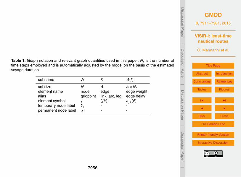
http://dx.doi.org/10.1080/1755876X.2015.1049892

GMDD8, 7911–7981, 2015


G. Mannarini et al.

Title Page



Tables Figures

J I

J I

Back Close

Full Screen / Esc



Discussion

Paper

|D

iscussionP

aper|

Discussion

Paper

|D

iscussionP

aper|

Table 1. Graph notation and relevant graph quantities used in this paper. Nt is the number oftime steps employed and is automatically adjusted by the model on the basis of the estimatedvoyage duration.

set name N E A(t)

set size N A A×Ntelement name node edge edge weightalias gridpoint link, arc, leg edge delayelement symbol j (jk) ajk(`)temporary node label Yj - -permanent node label Xj - -

7956





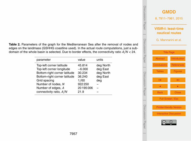
GMDD8, 7911–7981, 2015


G. Mannarini et al.

Title Page



Tables Figures

J I

J I

Back Close

Full Screen / Esc



Discussion

Paper

|D

iscussionP

aper|

Discussion

Paper

|D

iscussionP

aper|

Table 2. Parameters of the graph for the Mediterranean Sea after the removal of nodes andedges on the landmass (GSHHG coastline used). In the actual route computations, just a sub-domain of the whole basin is selected. Due to border effects, the connectivity ratio A/N < 24.

parameter value units

Top-left corner latitude 45.814 deg NorthTop-left corner longitude −6.000 deg EastBottom-right corner latitude 30.234 deg NorthBottom-right corner latitude 36.240 deg EastGrid spacing 1/60 degNumber of nodes, N 922 250 −Number of edges, A 20 195 006 −connectivity ratio, A/N 21.9 −

7957





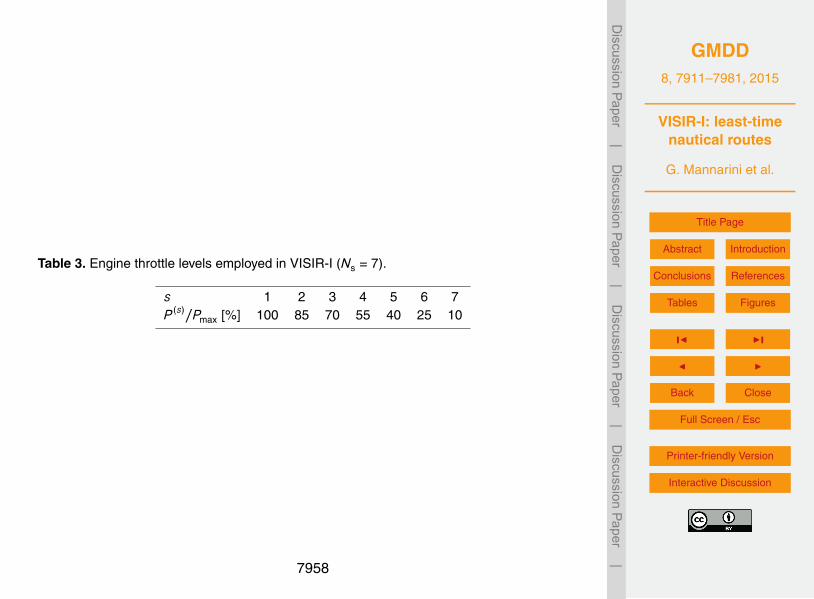
GMDD8, 7911–7981, 2015


G. Mannarini et al.

Title Page



Tables Figures

J I

J I

Back Close

Full Screen / Esc



Discussion

Paper

|D

iscussionP

aper|

Discussion

Paper

|D

iscussionP

aper|

Table 3. Engine throttle levels employed in VISIR-I (Ns = 7).

s 1 2 3 4 5 6 7P (s)/Pmax [%] 100 85 70 55 40 25 10

7958





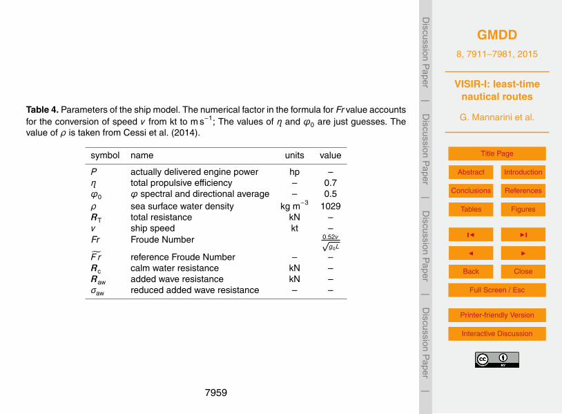
GMDD8, 7911–7981, 2015


G. Mannarini et al.

Title Page



Tables Figures

J I

J I

Back Close

Full Screen / Esc



Discussion

Paper

|D

iscussionP

aper|

Discussion

Paper

|D

iscussionP

aper|

Table 4. Parameters of the ship model. The numerical factor in the formula for Fr value accountsfor the conversion of speed v from kt to m s−1; The values of η and ϕ0 are just guesses. Thevalue of ρ is taken from Cessi et al. (2014).

symbol name units value

P actually delivered engine power hp –η total propulsive efficiency – 0.7ϕ0 ϕ spectral and directional average – 0.5ρ sea surface water density kg m−3 1029RT total resistance kN –v ship speed kt –Fr Froude Number 0.52v√

g0L

F r reference Froude Number – –Rc calm water resistance kN –Raw added wave resistance kN –σaw reduced added wave resistance – –

7959





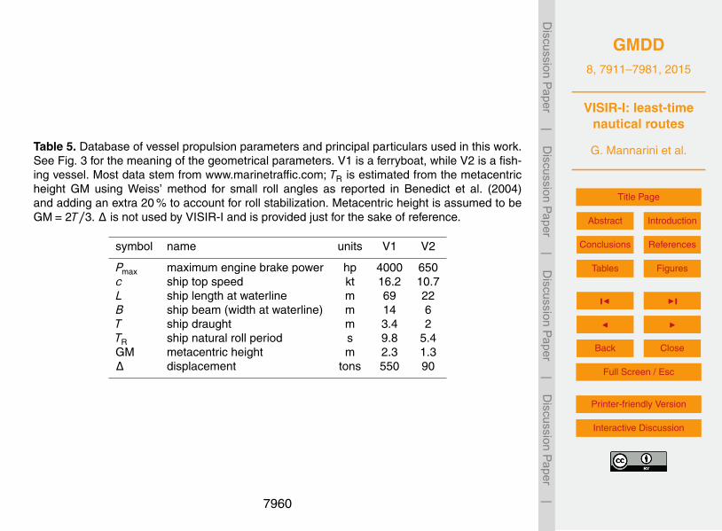
GMDD8, 7911–7981, 2015


G. Mannarini et al.

Title Page



Tables Figures

J I

J I

Back Close

Full Screen / Esc



Discussion

Paper

|D

iscussionP

aper|

Discussion

Paper

|D

iscussionP

aper|

Table 5. Database of vessel propulsion parameters and principal particulars used in this work.See Fig. 3 for the meaning of the geometrical parameters. V1 is a ferryboat, while V2 is a fish-ing vessel. Most data stem from www.marinetraffic.com; TR is estimated from the metacentricheight GM using Weiss’ method for small roll angles as reported in Benedict et al. (2004)and adding an extra 20 % to account for roll stabilization. Metacentric height is assumed to beGM= 2T/3. ∆ is not used by VISIR-I and is provided just for the sake of reference.

symbol name units V1 V2

Pmax maximum engine brake power hp 4000 650c ship top speed kt 16.2 10.7L ship length at waterline m 69 22B ship beam (width at waterline) m 14 6T ship draught m 3.4 2TR ship natural roll period s 9.8 5.4GM metacentric height m 2.3 1.3∆ displacement tons 550 90

7960





www.marinetraffic.com

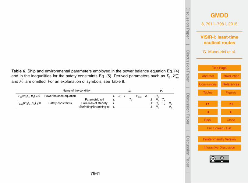
GMDD8, 7911–7981, 2015


G. Mannarini et al.

Title Page



Tables Figures

J I

J I

Back Close

Full Screen / Esc



Discussion

Paper

|D

iscussionP

aper|

Discussion

Paper

|D

iscussionP

aper|

Table 6. Ship and environmental parameters employed in the power balance equation Eq. (4)and in the inequalities for the safety constraints Eq. (5). Derived parameters such as TE, σaw

and F r are omitted. For an explanation of symbols, see Table 8.

Name of the condition ps pe

Feq(v ;ps,pe) = 0 Power balance equation L B T Pmax c HsParametric roll L TR λ Hs Tw

Fineq(v ;ps,pe) ≤ 0 Safety constraints Pure loss of stability L λ Hs Tw θwSurfriding/Broaching-to L λ Hs θw

7961





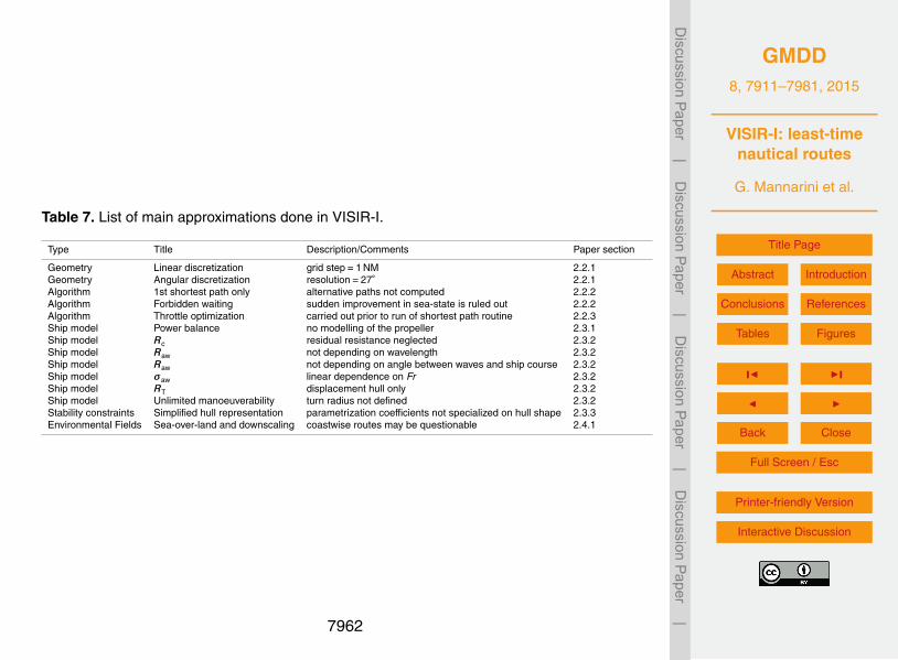
GMDD8, 7911–7981, 2015


G. Mannarini et al.

Title Page



Tables Figures

J I

J I

Back Close

Full Screen / Esc



Discussion

Paper

|D

iscussionP

aper|

Discussion

Paper

|D

iscussionP

aper|

Table 7. List of main approximations done in VISIR-I.

Type Title Description/Comments Paper section

Geometry Linear discretization grid step=1 NM 2.2.1Geometry Angular discretization resolution=27 2.2.1Algorithm 1st shortest path only alternative paths not computed 2.2.2Algorithm Forbidden waiting sudden improvement in sea-state is ruled out 2.2.2Algorithm Throttle optimization carried out prior to run of shortest path routine 2.2.3Ship model Power balance no modelling of the propeller 2.3.1Ship model Rc residual resistance neglected 2.3.2Ship model Raw not depending on wavelength 2.3.2Ship model Raw not depending on angle between waves and ship course 2.3.2Ship model σaw linear dependence on Fr 2.3.2Ship model RT displacement hull only 2.3.2Ship model Unlimited manoeuverability turn radius not defined 2.3.2Stability constraints Simplified hull representation parametrization coefficients not specialized on hull shape 2.3.3Environmental Fields Sea-over-land and downscaling coastwise routes may be questionable 2.4.1

7962





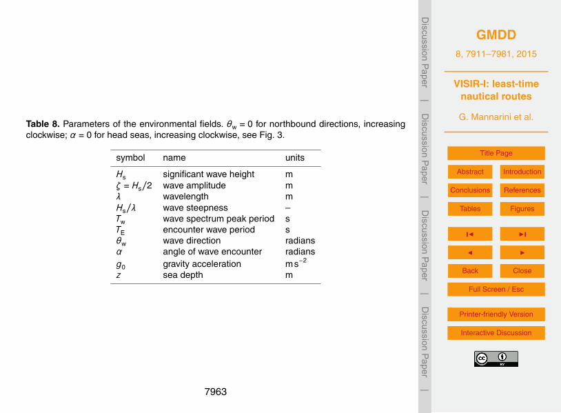
GMDD8, 7911–7981, 2015


G. Mannarini et al.

Title Page



Tables Figures

J I

J I

Back Close

Full Screen / Esc



Discussion

Paper

|D

iscussionP

aper|

Discussion

Paper

|D

iscussionP

aper|

Table 8. Parameters of the environmental fields. θw = 0 for northbound directions, increasingclockwise; α = 0 for head seas, increasing clockwise, see Fig. 3.

symbol name units

Hs significant wave height mζ = Hs/2 wave amplitude mλ wavelength mHs/λ wave steepness –Tw wave spectrum peak period sTE encounter wave period sθw wave direction radiansα angle of wave encounter radiansg0 gravity acceleration ms−2

z sea depth m

7963





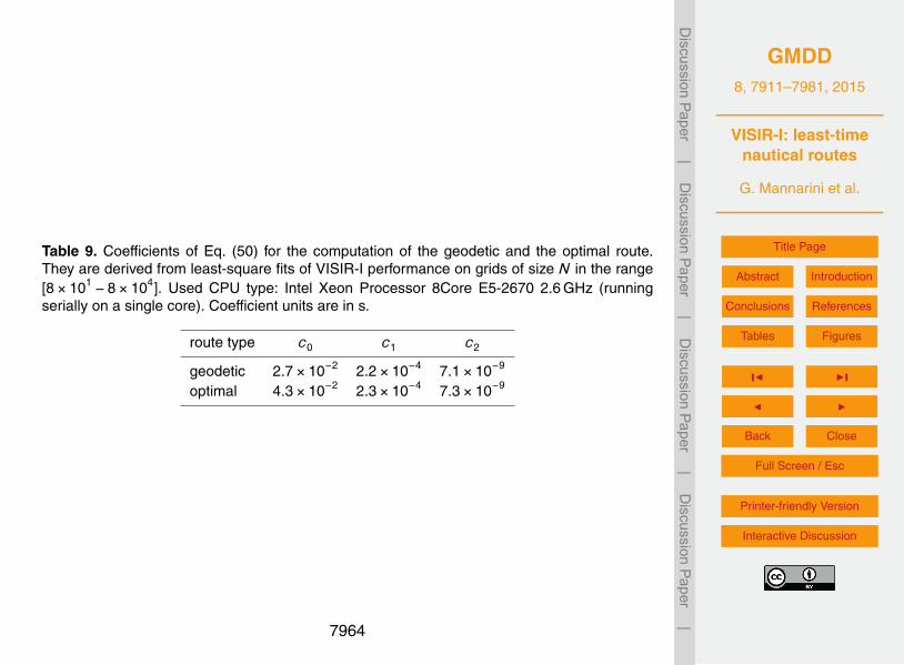
GMDD8, 7911–7981, 2015


G. Mannarini et al.

Title Page



Tables Figures

J I

J I

Back Close

Full Screen / Esc



Discussion

Paper

|D

iscussionP

aper|

Discussion

Paper

|D

iscussionP

aper|

Table 9. Coefficients of Eq. (50) for the computation of the geodetic and the optimal route.They are derived from least-square fits of VISIR-I performance on grids of size N in the range[8×101 −8×104]. Used CPU type: Intel Xeon Processor 8Core E5-2670 2.6 GHz (runningserially on a single core). Coefficient units are in s.

route type c0 c1 c2

geodetic 2.7×10−2 2.2×10−4 7.1×10−9

optimal 4.3×10−2 2.3×10−4 7.3×10−9

7964





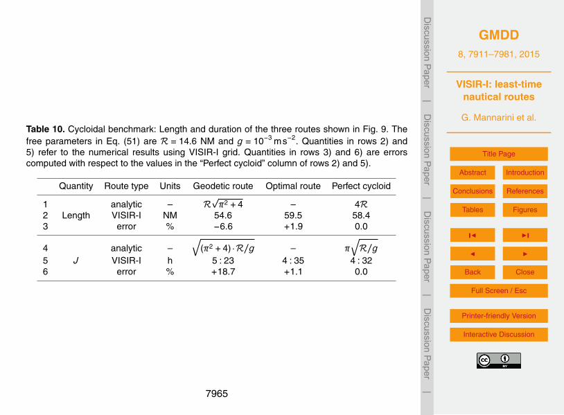
GMDD8, 7911–7981, 2015


G. Mannarini et al.

Title Page



Tables Figures

J I

J I

Back Close

Full Screen / Esc



Discussion

Paper

|D

iscussionP

aper|

Discussion

Paper

|D

iscussionP

aper|

Table 10. Cycloidal benchmark: Length and duration of the three routes shown in Fig. 9. Thefree parameters in Eq. (51) are R = 14.6 NM and g = 10−3 ms−2. Quantities in rows 2) and5) refer to the numerical results using VISIR-I grid. Quantities in rows 3) and 6) are errorscomputed with respect to the values in the “Perfect cycloid” column of rows 2) and 5).

Quantity Route type Units Geodetic route Optimal route Perfect cycloid

1 analytic – R√π2 +4 – 4R

2 Length VISIR-I NM 54.6 59.5 58.43 error % −6.6 +1.9 0.0

4 analytic –√

(π2 +4) · R/g – π√R/g

5 J VISIR-I h 5 : 23 4 : 35 4 : 326 error % +18.7 +1.1 0.0

7965





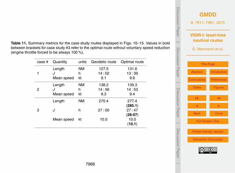
GMDD8, 7911–7981, 2015


G. Mannarini et al.

Title Page



Tables Figures

J I

J I

Back Close

Full Screen / Esc



Discussion

Paper

|D

iscussionP

aper|

Discussion

Paper

|D

iscussionP

aper|

Table 11. Summary metrics for the case study routes displayed in Figs. 10–15. Values in boldbetween brackets for case study #3 refer to the optimal route without voluntary speed reduction(engine throttle forced to be always 100 %).

case # Quantity units Geodetic route Optimal route

Length NM 127.5 131.61 J h 14 : 02 13 : 39

Mean speed kt 9.1 9.6

Length NM 138.2 139.32 J h 14 : 56 14 : 53

Mean speed kt 9.3 9.4

Length NM 270.4 277.4(285.1)

3 J h 27 : 00 27 : 47(28:07)

Mean speed kt 10.0 10.0(10.1)

7966





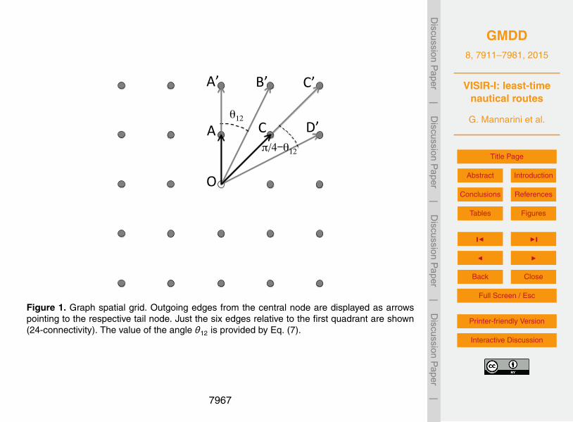
GMDD8, 7911–7981, 2015


G. Mannarini et al.

Title Page



Tables Figures

J I

J I

Back Close

Full Screen / Esc



Discussion

Paper

|D

iscussionP

aper|

Discussion

Paper

|D

iscussionP

aper|

O

A

A’ B’ C’

D’ C θ12

π/4-θ12

Figure 1. Graph spatial grid. Outgoing edges from the central node are displayed as arrowspointing to the respective tail node. Just the six edges relative to the first quadrant are shown(24-connectivity). The value of the angle θ12 is provided by Eq. (7).

7967





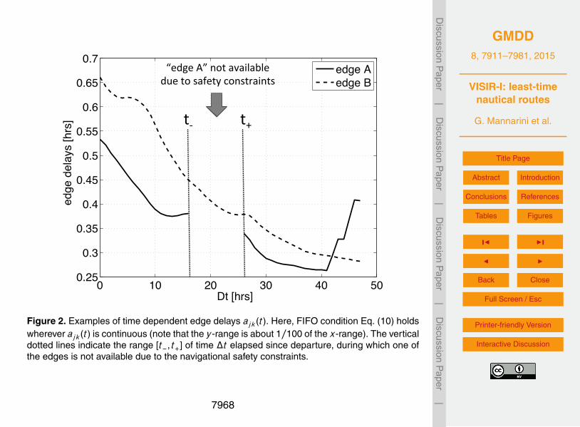
GMDD8, 7911–7981, 2015


G. Mannarini et al.

Title Page



Tables Figures

J I

J I

Back Close

Full Screen / Esc



Discussion

Paper

|D

iscussionP

aper|

Discussion

Paper

|D

iscussionP

aper|

0 10 20 30 40 500.25

0.3

0.35

0.4

0.45

0.5

0.55

0.6

0.65

0.7

Dt [hrs]

edge

del

ays

[hrs

]

edge Aedge B

t-‐ t+

“edge A” not available due to safety constraints

Figure 2. Examples of time dependent edge delays ajk(t). Here, FIFO condition Eq. (10) holdswherever ajk(t) is continuous (note that the y-range is about 1/100 of the x-range). The verticaldotted lines indicate the range [t−,t+] of time ∆t elapsed since departure, during which one ofthe edges is not available due to the navigational safety constraints.

7968





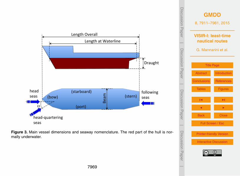
GMDD8, 7911–7981, 2015


G. Mannarini et al.

Title Page



Tables Figures

J I

J I

Back Close

Full Screen / Esc



Discussion

Paper

|D

iscussionP

aper|

Discussion

Paper

|D

iscussionP

aper|

Length Overall Length at Waterline

head seas

Draught

(starboard)

(port)

(stern) (bow) Be

am following

seas

α

head-‐quartering seas

Figure 3. Main vessel dimensions and seaway nomenclature. The red part of the hull is nor-mally underwater.

7969





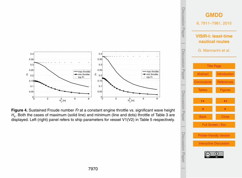
GMDD8, 7911–7981, 2015


G. Mannarini et al.

Title Page



Tables Figures

J I

J I

Back Close

Full Screen / Esc



Discussion

Paper

|D

iscussionP

aper|

Discussion

Paper

|D

iscussionP

aper|

0 2 4 6 80

0.05

0.1

0.15

0.2

0.25

0.3

0.35

0.4

Hs [m]

Fr

max throttlemin throttletop Fr

0 2 4 6 80

0.05

0.1

0.15

0.2

0.25

0.3

0.35

0.4

Hs [m]

Fr

max throttlemin throttletop Fr

Figure 4. Sustained Froude number Fr at a constant engine throttle vs. significant wave heightHs. Both the cases of maximum (solid line) and minimum (line and dots) throttle of Table 3 aredisplayed. Left (right) panel refers to ship parameters for vessel V1(V2) in Table 5 respectively.

7970





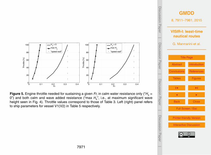
GMDD8, 7911–7981, 2015


G. Mannarini et al.

Title Page



Tables Figures

J I

J I

Back Close

Full Screen / Esc



Discussion

Paper

|D

iscussionP

aper|

Discussion

Paper

|D

iscussionP

aper|

0 0.1 0.2 0.3 0.40

20

40

60

80

100

Fr

Thro

ttle

[%]

Hs = 0max Hs"speed wall"

0 0.1 0.2 0.3 0.40

20

40

60

80

100

FrTh

rottl

e [%

]

Hs = 0max Hs"speed wall"

Figure 5. Engine throttle needed for sustaining a given Fr, in calm water resistance only (“Hs =0”) and both calm and wave added resistance (“max Hs”, i.e., at maximum significant waveheight seen in Fig. 4). Throttle values correspond to those of Table 3. Left (right) panel refersto ship parameters for vessel V1(V2) in Table 5 respectively.

7971





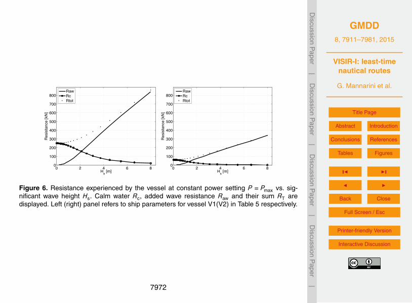
GMDD8, 7911–7981, 2015


G. Mannarini et al.

Title Page



Tables Figures

J I

J I

Back Close

Full Screen / Esc



Discussion

Paper

|D

iscussionP

aper|

Discussion

Paper

|D

iscussionP

aper|

0 2 4 6 80

100

200

300

400

500

600

700

800

Hs [m]

Res

ista

nce

[kN

]

RawRcRtot

0 2 4 6 80

100

200

300

400

500

600

700

800

Hs [m]

Res

ista

nce

[kN

]

RawRcRtot

Figure 6. Resistance experienced by the vessel at constant power setting P = Pmax vs. sig-nificant wave height Hs. Calm water Rc, added wave resistance Raw and their sum RT aredisplayed. Left (right) panel refers to ship parameters for vessel V1(V2) in Table 5 respectively.

7972





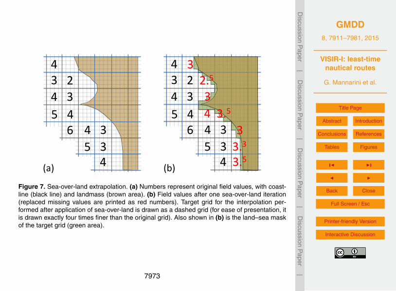
GMDD8, 7911–7981, 2015


G. Mannarini et al.

Title Page



Tables Figures

J I

J I

Back Close

Full Screen / Esc



Discussion

Paper

|D

iscussionP

aper|

Discussion

Paper

|D

iscussionP

aper|

4 2

6

3 4 3

4 5 3 4 3 5 4

4 2

6

3 4 3

4 5 3 4 3 5 4

3

3 4

2.5

3.3 3.5

3 3.5

(a) (b)

Figure 7. Sea-over-land extrapolation. (a) Numbers represent original field values, with coast-line (black line) and landmass (brown area). (b) Field values after one sea-over-land iteration(replaced missing values are printed as red numbers). Target grid for the interpolation per-formed after application of sea-over-land is drawn as a dashed grid (for ease of presentation, itis drawn exactly four times finer than the original grid). Also shown in (b) is the land–sea maskof the target grid (green area).

7973





GMDD8, 7911–7981, 2015


G. Mannarini et al.

Title Page



Tables Figures

J I

J I

Back Close

Full Screen / Esc



Discussion

Paper

|D

iscussionP

aper|

Discussion

Paper

|D

iscussionP

aper|

start

end

Sea nodes

Sea edges

Grid prepara/on

Fields regridding

Edge weights / Safety checks

Shortest paths (geode/c + op/mal)

1 2Ship speed LUT

Route info

Figure 8. Flow chart of the computer code of VISIR-I model. Functioning mode (1) is run justonce for preparing graph nodes and edges; mode (2) is the operational one, using sea nodesand edges computed from (1).

7974





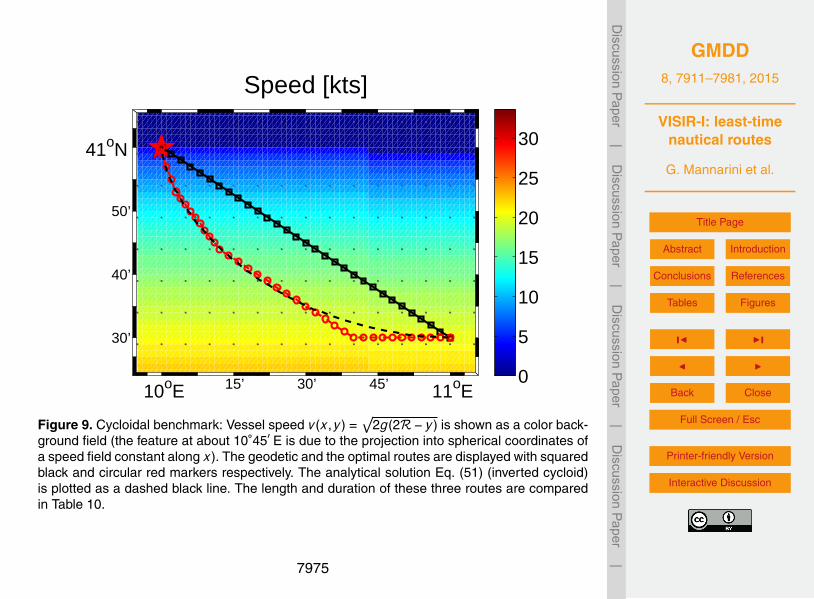
GMDD8, 7911–7981, 2015


G. Mannarini et al.

Title Page



Tables Figures

J I

J I

Back Close

Full Screen / Esc



Discussion

Paper

|D

iscussionP

aper|

Discussion

Paper

|D

iscussionP

aper|

Speed [kts]

10oE 15’ 30’ 45’ 11oE

30’

40’

50’

41oN

0

5

10

15

20

25

30

Figure 9. Cycloidal benchmark: Vessel speed v(x,y) =√

2g(2R− y) is shown as a color back-ground field (the feature at about 1045′ E is due to the projection into spherical coordinates ofa speed field constant along x). The geodetic and the optimal routes are displayed with squaredblack and circular red markers respectively. The analytical solution Eq. (51) (inverted cycloid)is plotted as a dashed black line. The length and duration of these three routes are comparedin Table 10.

7975





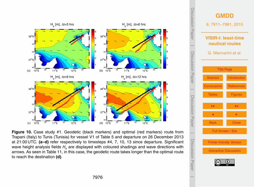
GMDD8, 7911–7981, 2015


G. Mannarini et al.

Title Page



Tables Figures

J I

J I

Back Close

Full Screen / Esc



Discussion

Paper

|D

iscussionP

aper|

Discussion

Paper

|D

iscussionP

aper|

10oE 30’ 11oE 30’ 12oE 30’ 40’

37oN

20’

40’

38oN

Hs [m], 6t=3 hrs

1

2

3

4

5

6

10oE 30’ 11oE 30’ 12oE 30’ 40’

37oN

20’

40’

38oN

Hs [m], 6t=9 hrs

1

2

3

4

5

6

10oE 30’ 11oE 30’ 12oE 30’ 40’

37oN

20’

40’

38oN

Hs [m], 6t=6 hrs

1

2

3

4

5

6

10oE 30’ 11oE 30’ 12oE 30’ 40’

37oN

20’

40’

38oN

Hs [m], 6t=12 hrs

1

2

3

4

5

6

(a)

(c)

(b)

(d)

Figure 10. Case study #1. Geodetic (black markers) and optimal (red markers) route fromTrapani (Italy) to Tunis (Tunisia) for vessel V1 of Table 5 and departure on 26 December 2013at 21:00 UTC. (a–d) refer respectively to timesteps #4, 7, 10, 13 since departure. Significantwave height analysis fields Hs are displayed with coloured shadings and wave directions witharrows. As seen in Table 11, in this case, the geodetic route takes longer than the optimal routeto reach the destination (d).

7976





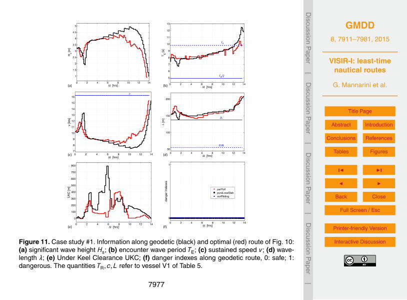
GMDD8, 7911–7981, 2015


G. Mannarini et al.

Title Page



Tables Figures

J I

J I

Back Close

Full Screen / Esc



Discussion

Paper

|D

iscussionP

aper|

Discussion

Paper

|D

iscussionP

aper|

0 2 4 6 8 10 12 14

1

1.5

2

2.5

3

3.5

4

4.5

5

Hs [m

]

6t [hrs] 0 2 4 6 8 10 12 14

5

6

7

8

9

10

11

12

13

T E [s]

6t [hrs]

0 2 4 6 8 10 12 147

8

9

10

11

12

13

14

15

16

v [k

ts]

6t [hrs]0 2 4 6 8 10 12 14

50

100

150

200

h [m

]

6t [hrs]

0 2 4 6 8 10 12 14

0

100

200

300

400

500

600

700

800

UKC

[m]

6t [hrs]0 2 4 6 8 10 12 14

0

1

6t [hrs]

dang

er In

dexe

s

parRollpureLossStabsurfRiding

(a) (b)

(c) (d)

(e) (f)

c

TR/2

TR

2L

0.8L

Figure 11. Case study #1. Information along geodetic (black) and optimal (red) route of Fig. 10:(a) significant wave height Hs; (b) encounter wave period TE; (c) sustained speed v ; (d) wave-length λ; (e) Under Keel Clearance UKC; (f) danger indexes along geodetic route, 0: safe; 1:dangerous. The quantities TR,c,L refer to vessel V1 of Table 5.

7977





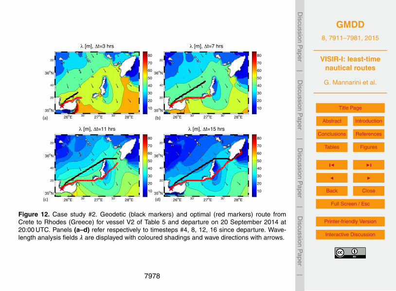
GMDD8, 7911–7981, 2015


G. Mannarini et al.

Title Page



Tables Figures

J I

J I

Back Close

Full Screen / Esc



Discussion

Paper

|D

iscussionP

aper|

Discussion

Paper

|D

iscussionP

aper|

26oE 30’ 27oE 30’ 28oE 35oN

20’

40’

36oN

20’

h [m], 6t=15 hrs

10

20

30

40

50

60

70

80

26oE 30’ 27oE 30’ 28oE 35oN

20’

40’

36oN

20’

h [m], 6t=11 hrs

10

20

30

40

50

60

70

80

26oE 30’ 27oE 30’ 28oE 35oN

20’

40’

36oN

20’

h [m], 6t=7 hrs

10

20

30

40

50

60

70

80

26oE 30’ 27oE 30’ 28oE 35oN

20’

40’

36oN

20’

h [m], 6t=3 hrs

10

20

30

40

50

60

70

80

(a)

(c)

(b)

(d)

Figure 12. Case study #2. Geodetic (black markers) and optimal (red markers) route fromCrete to Rhodes (Greece) for vessel V2 of Table 5 and departure on 20 September 2014 at20:00 UTC. Panels (a–d) refer respectively to timesteps #4, 8, 12, 16 since departure. Wave-length analysis fields λ are displayed with coloured shadings and wave directions with arrows.

7978





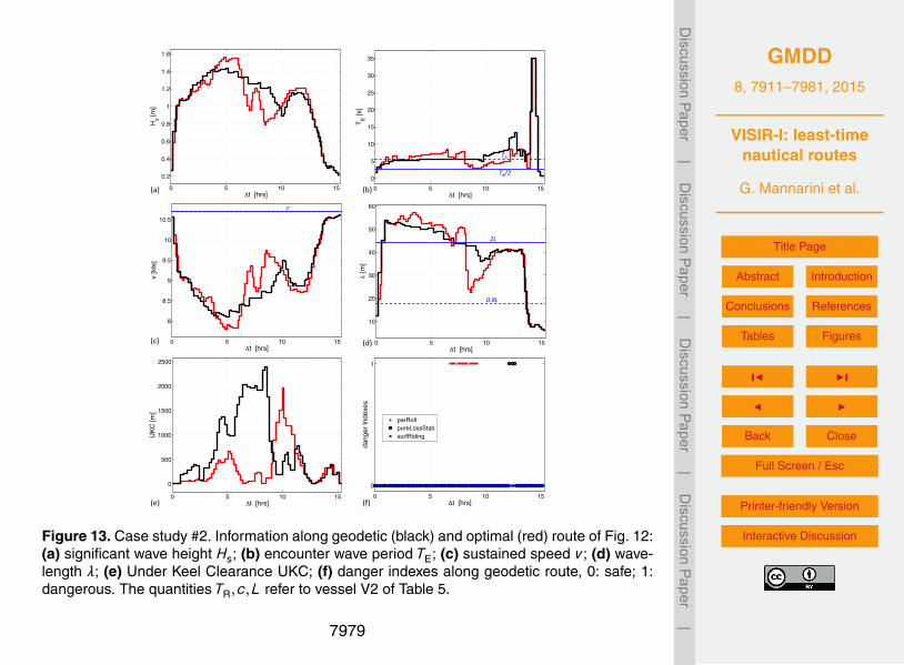
GMDD8, 7911–7981, 2015


G. Mannarini et al.

Title Page



Tables Figures

J I

J I

Back Close

Full Screen / Esc



Discussion

Paper

|D

iscussionP

aper|

Discussion

Paper

|D

iscussionP

aper|

0 5 10 15

0.2

0.4

0.6

0.8

1

1.2

1.4

1.6

Hs [m

]

6t [hrs]0 5 10 15

0

5

10

15

20

25

30

35

T E [s]

6t [hrs]

0 5 10 15

10

20

30

40

50

60

h [m

]6t [hrs]

0 5 10 15

8

8.5

9

9.5

10

10.5

v [k

ts]

6t [hrs]

0 5 10 15

0

500

1000

1500

2000

2500

UKC

[m]

6t [hrs]0 5 10 15

0

1

6t [hrs]

dang

er In

dexe

s


(a) (b)

(c) (d)

(e) (f)

c

TR/2

TR

2L

0.8L

Figure 13. Case study #2. Information along geodetic (black) and optimal (red) route of Fig. 12:(a) significant wave height Hs; (b) encounter wave period TE; (c) sustained speed v ; (d) wave-length λ; (e) Under Keel Clearance UKC; (f) danger indexes along geodetic route, 0: safe; 1:dangerous. The quantities TR,c,L refer to vessel V2 of Table 5.

7979





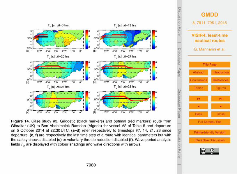
GMDD8, 7911–7981, 2015


G. Mannarini et al.

Title Page



Tables Figures

J I

J I

Back Close

Full Screen / Esc



Discussion

Paper

|D

iscussionP

aper|

Discussion

Paper

|D

iscussionP

aper|

5oW 4oW 3oW 2oW 1oW 0o 35oN

20’

40’ 36oN

20’

40’

Tw [s], 6t=27 hrs

2

4

6

8


20’

40’ 36oN

20’

40’

Tw [s], 6t=28 hrs

2

4

6

8


20’

40’ 36oN

20’

40’

Tw [s], 6t=26 hrs

2

4

6

8


20’

40’ 36oN

20’

40’

Tw [s], 6t=6 hrs

2

4

6

8

Tw [s], 6t=13 hrs


20’

40’ 36oN

20’

40’

2

4

6

8


20’

40’ 36oN

20’

40’

Tw [s], 6t=20 hrs

2

4

6

8

(a)

(c)

(b)

(d)

(e) (f)

Figure 14. Case study #3. Geodetic (black markers) and optimal (red markers) route fromGibraltar (UK) to Ben Abdelmalek Ramdan (Algeria) for vessel V2 of Table 5 and departureon 5 October 2014 at 22:30 UTC. (a–d) refer respectively to timesteps #7, 14, 21, 28 sincedeparture. (e, f) are respectively the last time step of a route with identical parameters but withthe safety checks disabled (e) or voluntary throttle reduction disabled (f). Wave period analysisfields Tw are displayed with colour shadings and wave directions with arrows.

7980





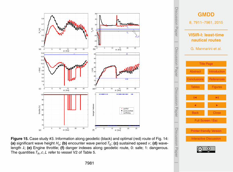
GMDD8, 7911–7981, 2015


G. Mannarini et al.

Title Page



Tables Figures

J I

J I

Back Close

Full Screen / Esc



Discussion

Paper

|D

iscussionP

aper|

Discussion

Paper

|D

iscussionP

aper|

0 5 10 15 20 250.3

0.4

0.5

0.6

0.7

0.8

Hs [m

]

6t [hrs]0 5 10 15 20 25

−60

−40

−20

0

20

40

60

T E [s]

6t [hrs]

0 5 10 15 20 25

70

75

80

85

90

95

100

thro

ttle

[%]

6t [hrs]

engine throttle [%]0 5 10 15 20 25

9

9.2

9.4

9.6

9.8

10

10.2

10.4

10.6

10.8

v [k

ts]

6t [hrs]0 5 10 15 20 25

10

15

20

25

30

35

40

45

h [m

]6t [hrs]

0 5 10 15 20 250

1

6t [hrs]

dang

er In

dexe

s


(a) (b)

(c) (d)

(e) (f)

c

±TR /2

TR

2L

0.8L

-‐TR

Figure 15. Case study #3. Information along geodetic (black) and optimal (red) route of Fig. 14:(a) significant wave height Hs; (b) encounter wave period TE; (c) sustained speed v ; (d) wave-length λ; (e) Engine throttle; (f) danger indexes along geodetic route, 0: safe; 1: dangerous.The quantities TR,c,L refer to vessel V2 of Table 5.

7981





Documents

VISIR-I: least-time nautical routes