Embed Size (px)
Citation preview

VISION-BASED ESTIMATION, LOCALIZATION, AND CONTROL OF ANUNMANNED AERIAL VEHICLE
By
MICHAEL KENT KAISER
A DISSERTATION PRESENTED TO THE GRADUATE SCHOOLOF THE UNIVERSITY OF FLORIDA IN PARTIAL FULFILLMENT
OF THE REQUIREMENTS FOR THE DEGREE OFDOCTOR OF PHILOSOPHY
UNIVERSITY OF FLORIDA
2008

Copyright 2008
by
Michael Kent Kaiser

To my wife, Brigita, our daughters, MaryEllen Ann and Eliška Gaynor, and my
mother, Carole Campbell Kaiser.

ACKNOWLEDGMENTS
First and foremost, I would like to express my gratitude to Dr. Warren Dixon
for not only providing me with exceptional guidance, encouragement, knowledge,
and friendship, but also serving as an example of a quality person of high character
- worthy of emulating!
I would also like to thank my committee members: Dr. Peter Ifju, Dr. Thomas
Burks, Dr. Norman Fitz-Coy, and Dr. Naira Hovakimyan. It was a great honor to
have them on my committee, each one carrying a specific meaning for me.
The NCR lab team is composed of a higher concentration of pure and lean
talent than any single group of people I have ever worked with, which is why it was
such a great privilege to be a member, albeit a little intimidating! I should point
out that those individuals in the NCR group who made my degree possible are:
Will MacKunis, Dr. Nick Gans, Dr. Guoqiang Hu, Parag Patre, and Sid Mehta.
And I would be remiss to not acknowledge the stabilizing "third leg" in
my schooling endeavors; namely, the Air Force Research Laboratory Munitions
Directorate (AFRL/RW) that provided the push and continued support for my
education.
Also of note, the following individuals whom I have had the opportunity to
work with as an engineer and who were either mentors or engineers to aspire to,
or both are: Henry Yarborough, Walter J. "Jake" Klinar, Dr. Karolos Grigoriadis,
Bob Loschke, Dr. Paul Bevilaqua, Dr. Leland Nicolai, John K. "Jack" Buckner, Dr.
James Cloutier, and Dr. Anthony Calise.
Finally, I cannot forget to mention Ms. Judi Shivers at the REEF and all of
the favors I owe her that I cannot possibly repay.
iv

TABLE OF CONTENTS
page
ACKNOWLEDGMENTS . . . . . . . . . . . . . . . . . . . . . . . . . . . . . iv
LIST OF FIGURES . . . . . . . . . . . . . . . . . . . . . . . . . . . . . . . . vii
ABSTRACT . . . . . . . . . . . . . . . . . . . . . . . . . . . . . . . . . . . . x
CHAPTER
1 INTRODUCTION . . . . . . . . . . . . . . . . . . . . . . . . . . . . . . 1
1.1 Motivation . . . . . . . . . . . . . . . . . . . . . . . . . . . . . . . . 11.2 Dissertation Overview . . . . . . . . . . . . . . . . . . . . . . . . . 61.3 Research Plan . . . . . . . . . . . . . . . . . . . . . . . . . . . . . . 6
2 AIRCRAFT MODELING AND SIMULATION . . . . . . . . . . . . . . 8
2.1 Introduction . . . . . . . . . . . . . . . . . . . . . . . . . . . . . . . 82.2 Aerodynamic Characterization . . . . . . . . . . . . . . . . . . . . . 92.3 Mass Property Estimation . . . . . . . . . . . . . . . . . . . . . . . 92.4 Simulink Effort . . . . . . . . . . . . . . . . . . . . . . . . . . . . . 132.5 Conclusions . . . . . . . . . . . . . . . . . . . . . . . . . . . . . . . 17
3 AUTONOMOUS CONTROL DESIGN . . . . . . . . . . . . . . . . . . . 18
3.1 Introduction . . . . . . . . . . . . . . . . . . . . . . . . . . . . . . . 183.2 Baseline Controller . . . . . . . . . . . . . . . . . . . . . . . . . . . 193.3 Robust Control Development . . . . . . . . . . . . . . . . . . . . . 213.4 Control Development . . . . . . . . . . . . . . . . . . . . . . . . . . 24
3.4.1 Error System . . . . . . . . . . . . . . . . . . . . . . . . . . 253.4.2 Stability Analysis . . . . . . . . . . . . . . . . . . . . . . . . 28
3.5 Simulation Results . . . . . . . . . . . . . . . . . . . . . . . . . . . 323.6 Conclusion . . . . . . . . . . . . . . . . . . . . . . . . . . . . . . . . 37
4 DAISY-CHAINING FOR STATE ESTIMATION . . . . . . . . . . . . . 39
4.1 Introduction . . . . . . . . . . . . . . . . . . . . . . . . . . . . . . . 394.2 Pose Reconstruction From Two Views . . . . . . . . . . . . . . . . 40
4.2.1 Euclidean Relationships . . . . . . . . . . . . . . . . . . . . . 404.2.2 Projective Relationships . . . . . . . . . . . . . . . . . . . . 414.2.3 Chained Pose Reconstruction for Aerial Vehicles . . . . . . . 424.2.4 Simulation Results . . . . . . . . . . . . . . . . . . . . . . . 47
v

4.2.5 Experimental Results . . . . . . . . . . . . . . . . . . . . . . 494.3 Conclusions . . . . . . . . . . . . . . . . . . . . . . . . . . . . . . . 61
5 LYAPUNOV-BASED STATE ESTIMATION . . . . . . . . . . . . . . . 63
5.1 Introduction . . . . . . . . . . . . . . . . . . . . . . . . . . . . . . . 635.2 Affine Euclidean Motion . . . . . . . . . . . . . . . . . . . . . . . . 635.3 Object Projection . . . . . . . . . . . . . . . . . . . . . . . . . . . . 665.4 Range Identification For Affine Systems . . . . . . . . . . . . . . . . 67
5.4.1 Objective . . . . . . . . . . . . . . . . . . . . . . . . . . . . . 675.4.2 Estimator Design and Error System . . . . . . . . . . . . . . 68
5.5 Analysis . . . . . . . . . . . . . . . . . . . . . . . . . . . . . . . . . 695.6 Conclusion . . . . . . . . . . . . . . . . . . . . . . . . . . . . . . . . 72
6 CONTRIBUTIONS AND FUTURE WORK . . . . . . . . . . . . . . . . 73
APPENDIX
A (CHAPTER 3) INTEGRATION OF THE AUXILIARY FUNCTION,L (t) . . . . . . . . . . . . . . . . . . . . . . . . . . . . . . . . . . . . . . 76
B (CHAPTER 4) VIDEO EQUIPMENT USED ONBOARD THE AIR-CRAFT . . . . . . . . . . . . . . . . . . . . . . . . . . . . . . . . . . . . 77
C (CHAPTER 4) GROUND SUPPORT EQUIPMENT . . . . . . . . . . . 81
REFERENCES . . . . . . . . . . . . . . . . . . . . . . . . . . . . . . . . . . . 84
BIOGRAPHICAL SKETCH . . . . . . . . . . . . . . . . . . . . . . . . . . . . 92
vi

LIST OF FIGURES
Figure page
2—1 LinAir wireframe representation of the Osprey airframe. . . . . . . . . . 9
2—2 Simulink modeling of aerodynamic coefficients. . . . . . . . . . . . . . . . 10
2—3 Measurable inertia values of the Osprey airframe. . . . . . . . . . . . . . 12
2—4 Simulink representation of the aircraft equations of motion. . . . . . . . . 15
2—5 Simulink aircraft equations of motion sub-block: Rotational EOM. . . . . 15
2—6 Simulink aircraft equations of motion sub-block: Body Rates to EulerAngle Rates. . . . . . . . . . . . . . . . . . . . . . . . . . . . . . . . . . 16
2—7 Simulink aircraft equations of motion sub-block: Translational EOM. . . 16
3—1 Photograph of the Osprey aircraft testbed. . . . . . . . . . . . . . . . . . 18
3—2 Rudimentary control system used for proof of concept for vision-basedextimation algorithms. . . . . . . . . . . . . . . . . . . . . . . . . . . . . 20
3—3 Plot of the discrete vertical (upward) wind gust used in the controllersimulation. . . . . . . . . . . . . . . . . . . . . . . . . . . . . . . . . . . 34
3—4 Illustration of uncoupled velocity and pitch rate response during closed-loop longitudinal controller operation. . . . . . . . . . . . . . . . . . . . 36
3—5 Illustration of uncoupled roll rate and yaw rate response during closed-loop lateral controller operation. . . . . . . . . . . . . . . . . . . . . . . . 37
4—1 Euclidean relationships between two camera poses. . . . . . . . . . . . . 41
4—2 Illustration of pose estimation chaining. . . . . . . . . . . . . . . . . . . . 44
4—3 Depth estimation from altitude. . . . . . . . . . . . . . . . . . . . . . . . 45
4—4 Actual translation versus estimated translation where the estimation isnot part of the closed-loop control. . . . . . . . . . . . . . . . . . . . . . 48
4—5 Actual attitude versus estimated attitude where the estimation is notpart of the closed-loop control. . . . . . . . . . . . . . . . . . . . . . . . 48
4—6 Autononmous control architecture. . . . . . . . . . . . . . . . . . . . . . 50
vii

4—7 Actual translation versus estimated translation where the estimated valueis used within the closed-loop control. . . . . . . . . . . . . . . . . . . . . 50
4—8 Actual attitude versus estimated attitude where the estimated value isused within the closed-loop control. . . . . . . . . . . . . . . . . . . . . . 51
4—9 Overview of the flight test system and component interconnections. . . . 52
4—10 Single video frame with GPS overlay illustrating landmarks placed alonginside edge of the runway. . . . . . . . . . . . . . . . . . . . . . . . . . . 52
4—11 Experimental flight test results. Estimated position compared to twoGPS signals. . . . . . . . . . . . . . . . . . . . . . . . . . . . . . . . . . . 53
4—12 Technique for achieving accurate landmark relative placement distances. 54
4—13 Single video frame from second flight test experiment illustrating the ef-fect of the more forward looking, wider field of view camera. . . . . . . . 55
4—14 Single video frame from second flight test experiment with the lens dis-tortion removed. . . . . . . . . . . . . . . . . . . . . . . . . . . . . . . . 56
4—15 Example of a 3D color contour plot generated from the matrix designedas a nonlinear combination of the red and green color space matrices. . . 57
4—16 Image plane trajectories made by the landmarks from patch 1 enterringand exiting the field of view. . . . . . . . . . . . . . . . . . . . . . . . . . 58
4—17 Basic concept of geometric position reconstruction from known landmarklocations. . . . . . . . . . . . . . . . . . . . . . . . . . . . . . . . . . . . 60
4—18 Illustration of how four tetrahedrons are used to estimate the length ofeach edge, a, b, c, & d three times. . . . . . . . . . . . . . . . . . . . . . 61
4—19 Second experimental flight test results. Estimated position compared tomore accurate position from geometric reconstruction technique. . . . . . 62
5—1 Moving camera stationary object scenario. . . . . . . . . . . . . . . . . . 65
5—2 Euclidean point projected onto image plane of a pinhole camera . . . . . 65
B—1 Sony Color Exview SuperHAD (480 Lines of Resolution) . . . . . . . . . 77
B—2 Panasonic AG-DV1 Digital Video Recorder . . . . . . . . . . . . . . . . . 78
B—3 Garmin GPS 35 OEM GPS Receiver . . . . . . . . . . . . . . . . . . . . 78
B—4 Intuitive Circuits, LLC - OSD-GPS Overlay Board . . . . . . . . . . . . 79
B—5 12V, 2.4Ghz, 100mW, Video Transmitter and Antennae . . . . . . . . . 79
viii

B—6 Eagle Tree, Seagull, Wireless Dashboard Flight System - Pro Version:(1) Wireless Telemetry Transmitter, (2) Eagle Tree Systems G-Force Ex-pander, and (3) Eagle Tree Systems GPS Expander . . . . . . . . . . . . 80
C—1 RX-2410 2.4 GHz Wireless 4-channel Audio/Video Selectable Receiver . 81
C—2 Sony GV-D1000 Portable MiniDV Video Walkman . . . . . . . . . . . . 82
C—3 Eagle Tree, Seagull, Real-time Data Dashboard, Wireless Telemetry Data,Receiver Model STR-01 . . . . . . . . . . . . . . . . . . . . . . . . . . . 82
C—4 Leica DISTOTM A5 (Measuring Range up to 650 ft, Accuracy +/- 0.06inches) . . . . . . . . . . . . . . . . . . . . . . . . . . . . . . . . . . . . . 83
ix

Abstract of Dissertation Presented to the Graduate Schoolof the University of Florida in Partial Fulfillment of theRequirements for the Degree of Doctor of Philosophy
VISION-BASED ESTIMATION, LOCALIZATION, AND CONTROL OF ANUNMANNED AERIAL VEHICLE
By
Michael Kent Kaiser
May 2008
Chair: Dr. Warren E. DixonMajor: Aerospace Engineering
Given the advancements in computer vision and estimation and control
theory, monocular camera systems have received growing interest as a local
alternative/collaborative sensor to GPS systems. One issue that has inhibited
the use of a vision system as a navigational aid is the difficulty in reconstructing
inertial measurements from the projected image. Current approaches to estimating
the aircraft state through a camera system utilize the motion of feature points
in an image. One geometric approach that is in this dissertation uses a series of
homography relationships to estimate position and orientation with respect to an
inertial pose. This approach creates a series of “daisy-chained” pose estimates in
which the current feature points can be related to previously viewed feature points
to determine the current coordinates between each successive image. Because this
technique relies on the accuracy of a depth estimation, a Lyapunov-based range
identification method is developed that is intended to enhance and compliment the
homography based method.
The nature of the noise associated with using a camera as a position and
orientation sensor is distinctly different from that of legacy type sensors used for air
x

vehicles such as accelerometers, rate gyros, attitude resolvers, etc. In order to fly an
aircraft in a closed-loop sense, using a camera as a primary sensor, the controller
will need to be robust to not only parametric uncertainties, but to system noise
that is of the kind uniquely characteristic of camera systems. A novel nonlinear
controller, capable of achieving asymptotic stability while rejecting a broad class of
uncertainties, is developed as a plausible answer to such anticipated issues.
A commercially available vehicle platform is selected to act as a testbed for
evaluating a host of image-based methodologies as well as evaluating advanced
control concepts. To enhance the vision-based analysis as well as control system
design analysis, a simulation of this particular aircraft is also constructed. The
simulation is intended to be used as a tool to provide insight into algorithm
feasibility as well as to support algorithm development, prior to physical integration
and flight testing.
The dissertation will focus on three problems of interest: 1) vehicle state
estimation and control using a homography-based daisy-chaining approach;
2) Lyapunov-based nonlinear state estimation and range identification using a
pinhole camera; 3) robust aerial vehicle control in the presence of structured and
unstructured uncertainties.
xi
CHAPTER 1INTRODUCTION
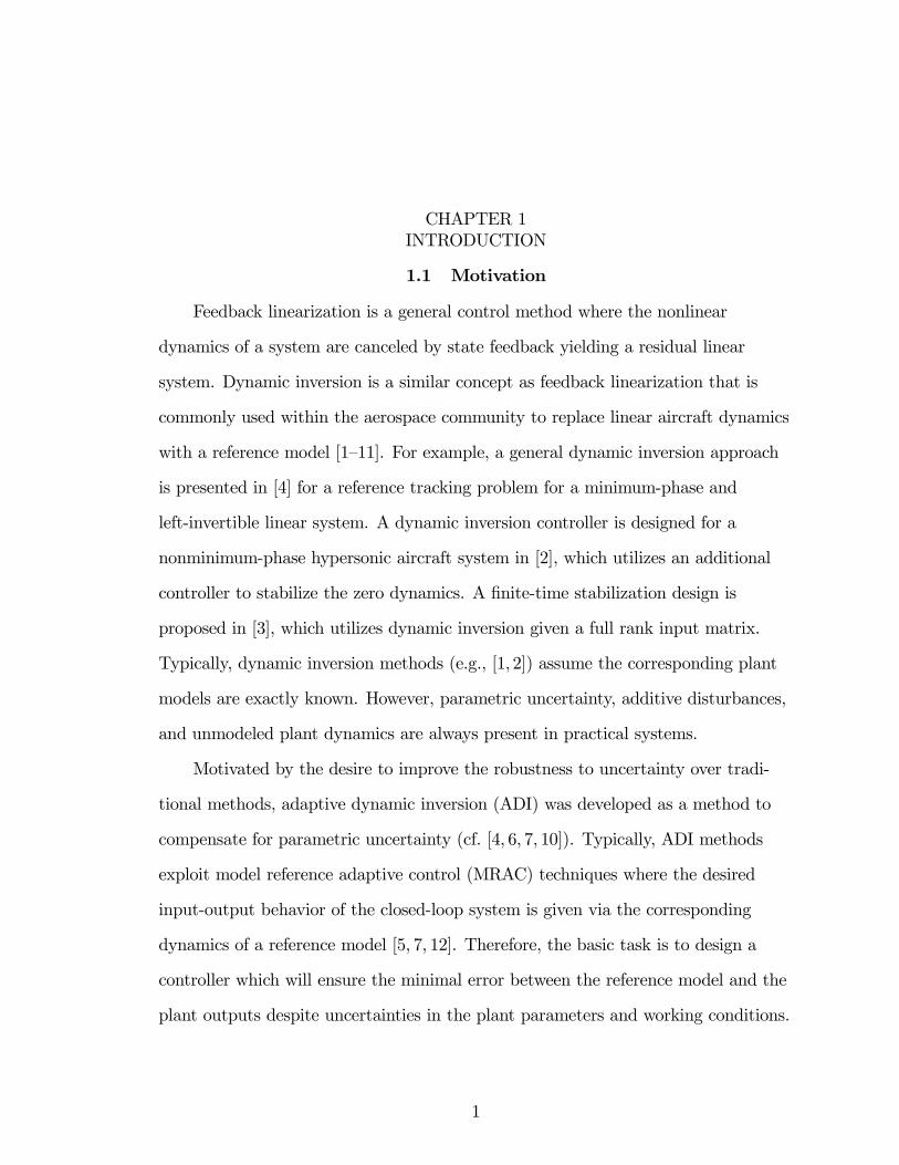
1.1 Motivation
Feedback linearization is a general control method where the nonlinear
dynamics of a system are canceled by state feedback yielding a residual linear
system. Dynamic inversion is a similar concept as feedback linearization that is
commonly used within the aerospace community to replace linear aircraft dynamics
with a reference model [1—11]. For example, a general dynamic inversion approach
is presented in [4] for a reference tracking problem for a minimum-phase and
left-invertible linear system. A dynamic inversion controller is designed for a
nonminimum-phase hypersonic aircraft system in [2], which utilizes an additional
controller to stabilize the zero dynamics. A finite-time stabilization design is
proposed in [3], which utilizes dynamic inversion given a full rank input matrix.
Typically, dynamic inversion methods (e.g., [1, 2]) assume the corresponding plant
models are exactly known. However, parametric uncertainty, additive disturbances,
and unmodeled plant dynamics are always present in practical systems.
Motivated by the desire to improve the robustness to uncertainty over tradi-
tional methods, adaptive dynamic inversion (ADI) was developed as a method to
compensate for parametric uncertainty (cf. [4, 6, 7, 10]). Typically, ADI methods
exploit model reference adaptive control (MRAC) techniques where the desired
input-output behavior of the closed-loop system is given via the corresponding
dynamics of a reference model [5, 7, 12]. Therefore, the basic task is to design a
controller which will ensure the minimal error between the reference model and the
plant outputs despite uncertainties in the plant parameters and working conditions.
1

2
Several efforts (e.g., [8—10, 13—16]) have been developed for the more general prob-
lem where the uncertain parameters or the inversion mismatch terms do not satisfy
the linear-in-the-parameters assumption (i.e., non-LP). One method to compen-
sate for non-LP uncertainty is to exploit a neural network as an on-line function
approximation method as in [13—15]; however, all of these results yield uniformly
ultimately bounded stability due to the inherent function reconstruction error.
In contrast to neural network-based methods to compensate for the non-LP
uncertainty, a robust control approach was recently developed in [17] (coined RISE
control in [18]) to yield an asymptotic stability result. The RISE-based control
structure has been used for a variety of fully actuated systems in [17—25]. The
contribution in this result is the use of the RISE control structure to achieve
asymptotic output tracking control of a model reference system, where the plant
dynamics contain a bounded additive disturbance (e.g., potential disturbances
include: gravity, inertial coupling, nonlinear gust modeling, etc.). This result
represents the first ever application of the RISE method where the controller
is multiplied by a non-square matrix containing parametric uncertainty. To
achieve the result, the typical RISE control structure and closed-loop error system
development is modified by adding a robust control term, which is designed to
compensate for the uncertainty in the input matrix. The result is proven via
Lyapunov-based stability analysis and demonstrated through numerical simulation.
GPS (Global Positioning System) is the primary navigational sensor modality
used for vehicle guidance, navigation, and control. However, a comprehensive
study referred to as the Volpe Report [26] indicates several vulnerabilities of GPS
associated with signal disruptions. The Volpe Report delineates the sources of
interference with the GPS signal into two categories, unintentional and deliberate
disruptions. Some of the unintentional disruptions include ionosphere interfer-
ence (also known as ionospheric scintillation) and radio frequency interference

3
(broadcast television, VHF, cell phones, two-way pagers); whereas, some of the
intentional disruptions involve jamming, spoofing, and meaconing. Some of the
ultimate recommendations of this report were to, “create awareness among mem-
bers of the domestic and global transportation community of the need for GPS
backup systems. . . ” and to “conduct a comprehensive analysis of GPS backup
navigation. . . ” which included ILS (Instrument Landing Systems), LORAN (LOng
RAnge Navigation), and INS (Inertial Navigation Systems) [26].
The Volpe report acted as an impetus to investigate mitigation strategies for
the vulnerabilities associated with the current GPS navigation protocol, nearly
all following the suggested GPS backup methods that revert to archaic/legacy
methods. Unfortunately, these navigational modalities are limited by the range
of their land-based transmitters, which are expensive and may not be feasible for
remote or hazardous environments. Based on these restrictions, researchers have
investigated local methods of estimating position when GPS is denied.
Given the advancements in computer vision and estimation and control
theory, monocular camera systems have received growing interest as a local
alternative/collaborative sensor to GPS systems. One issue that has inhibited
the use of a vision system as a navigational aid is the difficulty in reconstructing
inertial measurements from the projected image. Current approaches to estimating
the aircraft state through a camera system utilize the motion of feature points
in an image. A geometric approach is proposed in this dissertation that uses
a series of homography relationships to estimate position and orientation with
respect to an inertial pose. This approach creates a series of “daisy-chained” pose
estimates [27, 28] in which the current feature points can be related to previously
viewed feature points to determine the current coordinates between each successive
image. Through these relationships, previously recorded GPS data can be linked
with the image data to provide measurements of position and attitude (i.e. pose)

4
in navigational regions where GPS is denied. The method also delivers an accurate
estimation of vehicle attitude, which is an open problem in aerial vehicle control.
The estimation method can be executed in real time, making it amenable for use in
closed loop guidance control of an aircraft.
The concept of vision-based control for a flight vehicle has been an active
area of research over the last decade. Recent research literature on the subject of
vision-based state estimation for use in control of a flight vehicle can be categorized
by several distinctions. One distinction is that some methods rely heavily on
simultaneous sensor fusion [29] while other methods rely solely on camera feedback
[30]. Research can further be categorized into methods that require a priori
knowledge of landmarks (such as pattern or shape [31—36], light intensity variations
[37], runway edges or lights [38—40]) versus techniques that do not require any
prior knowledge of landmarks [41—47]. Another category of research includes
methods that require the image features to remain in the field-of-view [41] versus
methods that are capable of acquiring new features [42]. Finally, methods can be
categorized according to the vision-based technique for information extraction such
as: Optic Flow [48], Simultaneous Localization And Mapping (SLAM) [43], Stereo
Vision [49], Epipolar Geometry [34, 41, 45, 46]. This last category might also be
delineated between methods that are more computationally intensive and therefore
indicative of the level of real-time on-board computational feasibility.
Methods using homography relationships between images to estimate the
pose of an aircraft are presented by Caballero et al. [46] and Shakernia et al. [41]
(where it is referred to as the “planar essential matrix”). The method presented
by Caballero et al. is limited to flying above a planar environment and creates an
image mosaic, which can be costly in terms of memory. Shakernia’s approach, does
not account for feature points entering and exiting the camera field of view. The
method introduced in this dissertation proposes a solution which allows points to

5
continuously move into and out of the camera field of view. The requirement of
flying over a constant planar surface is also relaxed to allow flight over piecewise
planar patches, more characteristic of real world scenarios.
Reconstructing the Euclidean coordinates of observed feature points is a
challenging problem of significant interest , because range information (i.e.,
the distance from the imaging system to the feature point) is lost in the image
projection. Different tools (e.g., extended Kalman filter, nonlinear observers) have
been used to address the structure and/or motion recovery problem from different
points of view. Some researchers (e.g., see [50—53]) have applied the extended
Kalman filter (EKF) to address the structure/motion recovery problem. In order
to use the EKF method, a priori knowledge of the noise distribution is required,
and the motion recovery algorithm is developed based on the linearization of the
nonlinear vision-based motion estimation problem.
Due to restrictions with linear methods, researchers have developed various
nonlinear observers (e.g., see [54—58]). For example, several researchers have
investigated the range identification problem for conventional imaging systems
when the motion parameters are known. In [57], Jankovic and Ghosh developed
a discontinuous observer, known as the Identifier Based Observer (IBO), to
exponentially identify range information of features from successive images of a
camera where the object model is based on known skew-symmetric affine motion
parameters. In [55], Chen and Kano generalized the object motion beyond the
skew-symmetric form of [57] and developed a new discontinuous observer that
exponentially forced the state observation error to be uniformly ultimately bounded
(UUB). In comparison to the UUB result of [55], a continuous observer was
constructed in [56] to asymptotically identify the range information for a general
affine system with known motion parameters. That is, the result in [56] eliminated
the skew-symmetric assumption and yielded an asymptotic result with a continuous

6
observer. More recently, a state estimation strategy was developed in [59, 60] for
affine systems with known motion parameters where only a single homogeneous
observation point is provided (i.e., a single image coordinate). In [58], a reduced
order observer was developed to yield a semi-global asymptotic stability result for a
fixed camera viewing a moving object with known motion parameters for a pinhole
camera.
1.2 Dissertation Overview
In this dissertation, vision-based estimation, localization, and control method-
ologies are proposed for an autonomous air vehicle flying over what are nominally
considered as planar patches of feature points. The dissertation will focus on four
problems of interest: 1) develop a robust control system resulting in a semi-global
asymptotic stable system for an air vehicle with structured and unstructured
uncertainties; 2) provide a means of state estimation where feature points can
continuously enter and exit the field-of-view, as would nominally be the case for a
fixed-wing vehicle, via a novel daisy-chaining approach;. 3) introduce a vision-based
altimeter which seeks to resolve the depth ambiguity, which is a current issue with
the homography based daisy-chaining method that uses an altimeter to provide a
depth measurement.
1.3 Research Plan
This chapter serves as an introduction. The motivation, problem statement
and the proposed research plan of the dissertation is provided in this chapter.
Chapter 2 describes a from-the-ground-up simulation development of a
research air vehicle specifically selected for its performance capabilities for flight
testing of vision-based, estimation, localization, and control methodologies. An
outcome from this chapter is a fully nonlinear simulation of a commercially
available mini-aircraft that can be used for a wide range of analysis and design
purposes.

7
Chapter 3 presents an inner-loop robust control method, providing mathe-
matical theory and simulation results. The contribution of the development in
this chapter is a controller that is asymptotically stable for a broad class of model
uncertainties as well as bounded additive disturbances.
Chapter 4 involves the development of the daisy-chaining method as a viable
GPS backup technology as well as a state estimation procedure. Results are
demonstrated via simulation as well as flight testing. The contribution from this
chapter is in developing a means for an aircraft to perform position and orientation
estimation from planar feature point patches that enter and leave the field of view,
indefinitely.
Chapter 5 investigates a nonlinear estimator that can provide an alternate
means to altitude estimation as well as to provide alternate state estimation. The
results of this chapter is that it develops a Lyapunov-based nonlinear state esti-
mator using a pinhole camera that could work in symbiosis with the homography-
based daisy chaining technique and it also suggests how, at least notionally, the
camera can therefore be used as a sole sensor onboard an aircraft.

CHAPTER 2AIRCRAFT MODELING AND SIMULATION
2.1 Introduction
A vehicle simulation has been developed to investigate the feasibility of the
proposed vision-based state estimation and guidance method. The Osprey fixed
wing aerial vehicle, by Air and Sea Composites, Inc. (see Figure 4—3) was selected
for evaluating a host of image-based methodologies as well as for potentially
evaluating advanced control concepts. This particular aircraft was chosen for
several reasons; chiefly being: low cost, pusher prop being amenable to forward
looking camera placement, and payload capability. A fully nonlinear model of the
equations of motion and aerodynamics of the Osprey are constructed within the
Simulink framework. A nonlinear model, as opposed to linear model, is preferred in
this analysis as it better represents the coupled dynamics and camera kinematics,
which could potentially stress the performance and hence, feasibility of the pose
estimation algorithm.
The first undertaking of the dissertation is to develop a fully nonlinear, six
degrees-of-freedom model of the Osprey aircraft. The simulation will provide a
means to test proof-of-concept methodologies prior to testing on the actual Osprey
testbed. For example, a specific maneuver can be created within the simulation
environment to perform a simultaneous rolling, pitching, and yawing motion of
the aircraft combined with a fixed mounted camera to test the robustness of the
vision-based algorithm.
A commercially available vehicle platform is selected to act as a testbed for
evaluating a host of image-based methodologies as well as evaluating advanced
control concepts.
8

9
Figure 2—1: LinAir wireframe representation of the Osprey airframe.
2.2 Aerodynamic Characterization
The development of the vehicle simulation entailed two primary tasks, esti-
mating the aerodynamic characteristics and evaluating the mass properties. The
aerodynamic characterization of the Osprey aircraft was computed using LinAir, by
Desktop Aeronautics, Inc., which employs the discrete vortex Weissenger method
(i.e. extended lifting line theory), to solve the subsonic, inviscid, irrotational
Prandtl-Glauert equation [61]. Lifting surfaces are modeled by discrete horseshoe
vortices where each makes up one panel, panels make up an element, and elements
are grouped to make up the aircraft geometry as shown in Figure 2—1. The re-
sulting nondimensional, aerodynamic coefficients are implemented via Simulink’s
multi-dimensional lookup tables as illustrated in Figure 2—2.
2.3 Mass Property Estimation
The inertia and mass properties of the aircraft were measured using a precision
mass, center of gravity, and moment of inertia (MOI) instrument. The instru-
ment is comprised of a table levitated on a gas bearing pivot and a torsional rod
connected to the center of the table, resulting in a torsion pendulum for MOI
measurement. Because the vehicle could not be mounted on its nose or tail, an

10
Figure 2—2: Simulink modeling of aerodynamic coefficients.
alternate method was devised to estimate the vehicle’s roll inertia, Ixx. Given that
the angular momentum in one frame, A is related to angular momentum in a sec-
ond frame, B via a simple coordinate transformation, TAB (read as transformation
from frame B to frame A), the following series of relationships can be written
HA = TABH
B = TAB
£IBωB
¤= TA
B
£IB¡TBA T
AB
¢ωB¤
where¡TBA T
AB
¢= I
= TAB
£IBTB
A
¡TABω
B¢¤
where¡TABω
B¢= ωA
= TAB I
BTBA ω
A.
The inertia relationship between two frames is given by, IB = TAB I
BTBA , which for
this particular case of estimating the roll inertia is expressed as
⎡⎢⎢⎢⎢⎣Ixx 0 Ixz
0 Iyy 0
Ixz 0 Izz
⎤⎥⎥⎥⎥⎦ =⎡⎢⎢⎢⎢⎣
cθ 0 −sθ
0 1 0
sθ 0 cθ
⎤⎥⎥⎥⎥⎦⎡⎢⎢⎢⎢⎣
I 0xx 0 I 0xz
0 I 0yy 0
I 0xz 0 I 0zz
⎤⎥⎥⎥⎥⎦⎡⎢⎢⎢⎢⎣
cθ 0 sθ
0 1 0
−sθ 0 cθ
⎤⎥⎥⎥⎥⎦ (2—1)

11
Expanding this equation
⎡⎢⎢⎢⎢⎣Ixx 0 Ixz
0 Iyy 0
Ixz 0 Izz
⎤⎥⎥⎥⎥⎦ =
⎡⎢⎢⎢⎢⎢⎢⎢⎢⎢⎢⎢⎣
I 0xx cos2 (θ)− I 0xz sin (2θ) . . .
+I 0zz sin2 (θ)
0I 0xxsin (2θ)
2+ I 0xz cos (2θ) . . .
−I 0zzsin (2θ)
2
0 I 0yy 0
I 0xxsin (2θ)
2+ I 0xz cos (2θ) . . .
−I 0zzsin (2θ)
2
0I 0xx sin
2 (θ) + I 0xz sin (2θ) . . .
+I 0zz cos2 (θ)
⎤⎥⎥⎥⎥⎥⎥⎥⎥⎥⎥⎥⎦(2—2)
From this, it is noted that Iyy = I 0yy, as expected. Furthermore, because the
airframe is mostly symmetrical about its x-y plane, see Figure 2—3, it is reasonable
to assume that Ixz ≈ 0. Notice also that since the matrix in (2—2) is symmetric, it
is only necessary to look at the upper or lower triangular elements. Separating the
known terms on the right-hand-side and unknown terms on the left-hand-side gives
the following equalities
Ixx − I 0xx cos2 (θ) + I 0xz sin (2θ) = I 0zz sin
2 (θ)
−I 0xx sin2 (θ)− I 0xz sin (2θ) = −Izz + I 0zz cos2 (θ)
I 0xxsin (2θ)
2+ I 0xz cos (2θ) = I 0zz
sin (2θ)
2(2—3)
Rewriting in matrix form, the unknown terms are solved for accordingly
⎧⎪⎪⎪⎪⎨⎪⎪⎪⎪⎩Ixx
I 0xx
I 0xz
⎫⎪⎪⎪⎪⎬⎪⎪⎪⎪⎭ =
⎡⎢⎢⎢⎢⎣1 − cos2 (θ) sin (2θ)
0 − sin2 (θ) − sin (2θ)
0sin (2θ)
2cos (2θ)
⎤⎥⎥⎥⎥⎦−1⎧⎪⎪⎪⎪⎨⎪⎪⎪⎪⎩
I 0zz sin2 (θ)
−Izz + I 0zz cos2 (θ)
I 0zzsin (2θ)
2
⎫⎪⎪⎪⎪⎬⎪⎪⎪⎪⎭ (2—4)
The known terms in (2—4) are I 0zz, Izz, and θ, where θ is as depicted in Figure
2—3. Therefore, the complete inertia properties can be calculated from the only 3
measurements possible, as illustrated in Figure 2—3.

12
Figure 2—3: Measurable inertia values of the Osprey airframe.

13
2.4 Simulink Effort
The core of the simulation uses the aforementioned aerodynamics and mass
properties along with the following nonlinear translational and rotational rigid
body equations of motion derived in the vehicle body-axis system
u =1
mFx (V, ρ, α, q, δelev, δthrot)− qw + rv − g sin (θ) (2—5)
v =1
mFy (V, ρ, α, β, p, r)− ru+ pw + g cos (θ) sin (φ) (2—6)
w =1
mFz (V, ρ, α, q)− pv + qu+ g cos (θ) cos (φ) (2—7)
and
p =Izz
IxxIzz − I2xzMx (V, ρ, α, β, p, r, δrud, δail) +
IzzIxxIzz − I2xz
−qr (Izz − Iyy) + Ixzpq . . .
+Ixz
IxxIzz − I2xzMz (V, ρ, α, β, p, r, δrud, δail) +
IxzIxxIzz − I2xz
−pq (Iyy − Ixx)− Ixzqr
(2—8)
q =1
IyMy (V, ρ, α, q, δelev)− rp (Ixx − Izz)− Ixz
¡p2 − r2
¢(2—9)
r =Ixz
IxxIzz − I2xzMx (V, ρ, α, β, p, r, δrud, δail) +
IxzIxxIzz − I2xz
−qr (Izz − Iyy) + Ixzpq . . .
+Ixx
IxxIzz − I2xzMz (V, ρ, α, β, p, r, δrud, δail) +
IxxIxxIzz − I2xz
−pq (Iyy − Ixx)− Ixzqr
(2—10)
where M and F represent the aerodynamic and propulsive moments and forces in
body axis, given in x, y, & z components; I and m represent the vehicle’s inertia
tensor values and mass; V and ρ are relative velocity and air density; α and β are
angle of attack and sideslip angle; p, q, and r are angular body rates; u, v, and
w are translational velocities in the body frame; and δ represents the individual

14
control deflections. The corresponding kinematic relationships are given by⎡⎢⎢⎢⎢⎣X
Y
Z
⎤⎥⎥⎥⎥⎦ =⎡⎢⎢⎢⎢⎣
cθcψ sφsθcψ − cφsψ
cθsψ sφsθsψ + cφcψ
−sθ sφcθ
cφsθcψ + sφsψ
cφsθsψ − sφcψ
cφcθ
⎤⎥⎥⎥⎥⎦⎡⎢⎢⎢⎢⎣
u
v
w
⎤⎥⎥⎥⎥⎦ (2—11)
and ⎡⎢⎢⎢⎢⎣φ
θ
ψ
⎤⎥⎥⎥⎥⎦ =⎡⎢⎢⎢⎢⎣1 sinφ tan θ cosφ tan θ
0 cosφ − sinφ
0 sinφ sec θ cosφ sec θ
⎤⎥⎥⎥⎥⎦⎡⎢⎢⎢⎢⎣
p
q
r
⎤⎥⎥⎥⎥⎦ (2—12)
where cψ and sψ denote cos(ψ) and sin(ψ), respectively (similarly for φ and θ).
The equations of motion and all simulation subsystems are constructed using
standard Simulink library blocks, where no script files are incorporated, as shown
in Figure 2—4.
The sub-blocks of interest depicted in the equations of motion model given
in Figure 2—4 are: “Rotational EOM”, “Body Rates to Euler Angle Rates”, and
“Translational EOM”, and are illustrated in Figures 2—5, 2—6, and 2—7, respectively.
Besides using the model given in Figure 2—4 for cases where a fully nonlinear
simulation is required, it can also be used to generate linearized representations of
the Osprey by utilizing Matlab’s linearizing capability. For example, the trimmed
vehicle at a 60 meter altitude at 25 meters/sec. would have the corresponding state
space representation
⎡⎢⎢⎢⎢⎢⎢⎢⎣
V
α
q
θ
⎤⎥⎥⎥⎥⎥⎥⎥⎦=
⎡⎢⎢⎢⎢⎢⎢⎢⎣
−0.15 11.08 0.08 −9.81
−0.03 −7.17 0.83 0
0 −37.35 −9.96 0
0 0 1.00 0
⎤⎥⎥⎥⎥⎥⎥⎥⎦
⎡⎢⎢⎢⎢⎢⎢⎢⎣
V
α
q
θ
⎤⎥⎥⎥⎥⎥⎥⎥⎦+
⎡⎢⎢⎢⎢⎢⎢⎢⎣
3E−3 0.06
1E−5 1E−4
−0.98 0
0 0
⎤⎥⎥⎥⎥⎥⎥⎥⎦⎡⎢⎣ δelevator
δthrust
⎤⎥⎦(2—13)

15
1(12) ratesstates (12)
pqr
Phi_Theta_Psi
uv w
xy z
split upstates
pqr
Forces
uv w
mass
uv w dot
TranslationalEOM
Total_Torques
pqr
Inertia Matrix
pqr dot
RotationalEOM
Transf orm_Matrix
xy zXYZ
Position
Mux
pqr
Phi_Theta_PsiPhi_Theta_Psi dot
Body Rates toEuler Angle Rates
6states (12)
5Transform_Matrix
4Inertia Matrix
3mass
2
Total Forces (@cg)
1
Total Torques (@cg)
Figure 2—4: Simulink representation of the aircraft equations of motion.
H cross Omega
inv(I)*H_dot = omega_dot
1
pqr dot
Transf orm_Matrix
xy zXYZ
Matrix Multiplication2
Transf orm_Matrix
xy zXYZ
Matrix Multiplication
Matrix Inv _Matrix
Invert 3x3
H_dot
A
BA_cross_B
Cross Product
3Inertia Matrix
2
pqr 1
Total_Torques
Figure 2—5: Simulink aircraft equations of motion sub-block: Rotational EOM.

16
1
Phi_Theta_Psi dot
u[2]*u[7] - u[3]*u[6]
Theta_Dot
sin(u[1])
Sin_Theta
sin(u[1])
Sin_Phi
(u[2]*u[6] + u[3]*u[7])/u[5]
Psi_Dot
u[1] + u[2]*u[6]*u[4]/u[5] + u[3]*u[7]*u[4]/u[5]
Phi_Dot
Mux Mux
Euler_Rates
em cos(u[1])
Cos_Theta
cos(u[1])
Cos_Phi
2
Phi_Theta_Psi
1
pqr
Figure 2—6: Simulink aircraft equations of motion sub-block: Body Rates to EulerAngle Rates.
1
uvw dot
Mux
uvw_Dot
Mux
u[3]/u[10] - u[8]*u[4] + u[7]*u[5]
Accel_minus_Cross_z (w_dot)
u[2]/u[10] - u[7]*u[6] + u[9]*u[4]
Accel_minus_Cross_y (v_dot)
u[1]/u[10] - u[9]*u[5] + u[8]*u[6]
Accel_minus_Cross_x (u_dot)
4mass
3
uvw
2
Forces
1
pqr
Figure 2—7: Simulink aircraft equations of motion sub-block: Translational EOM.

17
And the corresponding lateral state-space representation is computed to be⎡⎢⎢⎢⎢⎢⎢⎢⎣
β
p
r
φ
⎤⎥⎥⎥⎥⎥⎥⎥⎦=
⎡⎢⎢⎢⎢⎢⎢⎢⎣
−0.69 −0.03 −0.99 0.39
−3.13 −12.92 1.10 0
17.03 −0.10 −0.97 0
0 1.00 −0.03 0
⎤⎥⎥⎥⎥⎥⎥⎥⎦
⎡⎢⎢⎢⎢⎢⎢⎢⎣
β
p
r
φ
⎤⎥⎥⎥⎥⎥⎥⎥⎦+
⎡⎢⎢⎢⎢⎢⎢⎢⎣
0 0
1.50 −0.02
−0.09 0.17
0 0
⎤⎥⎥⎥⎥⎥⎥⎥⎦⎡⎢⎣ δaileron
δrudder
⎤⎥⎦(2—14)
where ⎡⎢⎢⎢⎢⎢⎢⎢⎣
V = m/sec
α = rad
q = rad/sec
θ = rad
⎤⎥⎥⎥⎥⎥⎥⎥⎦,
⎡⎢⎢⎢⎢⎢⎢⎢⎣
β = rad
p = rad/sec
r = rad/sec
φ = rad
⎤⎥⎥⎥⎥⎥⎥⎥⎦, and
⎡⎢⎢⎢⎢⎢⎢⎢⎣
δelevator = deg
δthrust = N
δaileron = deg
δrudder = deg
⎤⎥⎥⎥⎥⎥⎥⎥⎦This model would provide useful information in regards to intermediate
feasibility of the vision-based method, such as providing insight into motion and
frequency issues which can severely affect the performance of the vision-based
methods. It can also serve as a basis for rudimentary control design, in the case
where the flight regime is benign and hence, does not require emphasize the effect
of vision-based state estimation in regards to vehicle control.
2.5 Conclusions
The efforts in this chapter illustrated the ground up development of a fully
nonlinear simulation representing an aircraft testbed to host flight testing of
image-based estimation and control algorithms. A method was devised to estimate
the vehicle’s roll inertia properties based upon the fact that the vehicle, unlike
most airframes, is relatively symmetrical about its x-y plane. Finally, while the
aerodynamic parameter estimates are derived from commercially available vortex
lattice software, this type of code is very beneficial in time and cost savings, but it
comes at the cost of model uncertainty; which yet again calls for control algorithms
that are inherently robust.

CHAPTER 3AUTONOMOUS CONTROL DESIGN
3.1 Introduction
A robust control approach was recently developed in [17] that exploits a
unique property of the integral of the sign of the error (coined RISE control in [18])
to yield an asymptotic stability result. The RISE based control structure has been
used for a variety of fully actuated systems in [17], [18], [62]. The contribution of
this result is the ability to achieve asymptotic tracking control of a model reference
system for not only a broad class of model uncertainties, but also for where the
plant dynamics contain a bounded additive disturbance (e.g., potential disturbances
include: dynamic inversion mismatch, wind gusts, nonlinear dynamics, etc.). In
addition, this result represents the first ever application of the RISE method
where the controller is multiplied by a non-square matrix containing parametric
uncertainty and nonlinear, non-LP disturbances. The feasibility of this technique
is proven through a Lyapunov-based stability analysis and through numerical
simulation results.
Figure 3—1: Photograph of the Osprey aircraft testbed.
18

19
3.2 Baseline Controller
As mentioned, the vision-based estimation method the will be discussed
further in chapter 4 was be experimentally demonstrated by flight testing with an
Osprey Aircraft. Prior to performing the experiment, the aircraft was modelled
and the estimation method was tested in simulation. A Simulink modeling effort
has been undertaken to develop a fully nonlinear, six degrees-of-freedom model
of an Osprey aircraft. A simplified autopilot design is constructed, with inputs
complimentary with the outputs from the estimation method, and a specific
maneuver is created to perform a simultaneous rolling, pitching, and yawing motion
of the aircraft combined with a fixed mounted camera. The aircraft/autopilot
modeling effort and maneuver is intended to test the robustness of the vision-based
algorithm as well as to provide proof-of-concept in using the camera as the primary
sensor for achieving closed-loop autonomous flight.
With the vehicle model as described, a baseline autopilot is incorporated to
allow for the vehicle to perform simple commanded maneuvers that an autonomous
aircraft would typically be expected to receive from an on-board guidance sys-
tem. The autopilot architecture, given in Figure 3—2, is specifically designed to
accept inputs compatible with the state estimates coming from the vision-based
algorithms. Preliminary modal analysis of the Osprey vehicle flying at a 60 meter
altitude at 25 meters/sec indicated a short-period frequency, ωsp = 10.1 rad/sec and
damping, ζsp = 0.85; a phugoid mode frequency, ωph = 0.34 rad/sec and damping,
ζph = 0.24; a dutch-roll frequency, ωdr = 4.20 rad/sec and damping, ζdr = 0.19; a
roll subsidence time constant of τ = 0.08 sec.; and a spiral mode time-to-double,
ttd = 44.01 sec. These values, which correspond to (2—13) and (2—14), are crucial
for the auto-pilot design as well as in determining what, if any, of the state esti-
mation values coming from the camera and proposed technique are favorable to

20
Y
cmdY PI
FilterWashout
YK
YK.φK ailδ+
-
+
+
+
-
+
-
φ
φ.
rFilter
WashoutYK rudδ
H
cmdH PI
FilterWashout
HK
HK .θK elevδ+
-
+
+
+
-
θ
V
cmdVPI VK+
-throtδ
φK.
Figure 3—2: Rudimentary control system used for proof of concept for vision-basedextimation algorithms.
be used in a closed-loop sense, as video frame rate and quantization noise become
integral to the controller design from a frequency standpoint.
As the aircraft, with an integrated vision-based system, is required to fly in
lesser benign regimes, such as maneuvering in and around structures, it becomes
evident that simplistic classical control methods will be limited in performance
capabilities. The aircraft system under consideration can be modeled via the
following state space representation [2,6,11,63,64]:
x = Ax+Bu+ f (x, t) (3—1)
y = Cx, (3—2)
21
where A ∈ Rn×n denotes the state matrix, B ∈ Rn×m for m < n represents the
input matrix, C ∈ Rm×n is the known output matrix, u ∈ Rm is a vector of control
inputs, and f (x, t) ∈ Rn represents an unknown, nonlinear disturbance.
Assumption 1: The A and B matrices given in (3—1) contain parametric
uncertainty.
Assumption 2: The nonlinear disturbance f (x, t) and its first two time
derivatives are assumed to exist and be bounded by a known constant.
3.3 Robust Control Development
In this section, it is described how a specific aircraft can be related to (3—1).
Based on the standard assumption that the longitudinal and lateral modes of the
aircraft are decoupled, the state space model for the Osprey aircraft testbed can
be represented using (3—1) and (3—2), where the state matrix A ∈ R8×8 and input
matrix B ∈ R8×4 given in chapter 2 are expressed as
A =
⎡⎢⎣ Alon 04×4
04×4 Alat
⎤⎥⎦ B =
⎡⎢⎣ Blon 04×2
04×2 Blat
⎤⎥⎦ , (3—3)
and the output matrix C ∈ R4×8 is designed as
C =
⎡⎢⎣ Clon 02×4
02×4 Clat
⎤⎥⎦ , (3—4)
where Alon, Alat ∈ R4×4, Blon, Blat ∈ R4×2, and Clon, Clat ∈ R2×4 denote the state
matrices, input matrices, and output matrices, respectively, for the longitudinal
and lateral subsystems, and the notation 0i×j denotes an i× j matrix of zeros. The
state vector x(t) ∈ R8 is given as
x =
∙xTlon xTlat
¸T, (3—5)

22
where xlon (t) , xlat (t) ∈ R4 denote the longitudinal and lateral state vectors defined
as
xlon ,∙V α q θ
¸T(3—6)
xlat ,∙β p r φ
¸T, (3—7)
where the state variables are defined as
V = velocity α = angle of attack
q = pitch rate θ = pitch angle
β = sideslip angle p = roll rate
r = yaw rate φ = bank angle
and the control input vector is defined as
u ,∙uTlon uTlat
¸T(3—8)
=
∙δelev δthrust δail δrud
¸T.
In (3—8), δelev (t) ∈ R denotes the elevator deflection angle, δthrust (t) ∈ R is the
control thrust, δail (t) ∈ R is the aileron deflection angle, and δrud (t) ∈ R is the
rudder deflection angle.
The disturbance f (x, t) introduced in (3—1) can represent several bounded
nonlinearities. The more promising example of disturbances that can be repre-
sented by f (x, t) is the nonlinear form of a selectively extracted portion of the
state space matrix Alon ∈ R4×4 that would normally be linearized. This nonlinearity
would then be added to the new state space plant by superposition, resulting in the
following quasi-linear plant model:
xlon = A0lonxlon +Blonulon + f (xlon, t) , (3—9)

23
where A0lon ∈ R4×4 is the state space matrix Alon with the linearized portion
removed, and f (xlon, t) ∈ R4 denotes the nonlinear disturbances present in the
longitudinal dynamics. Some physical examples of f (xlon, t) would be the selective
nonlinearities that cannot be ignored, such as when dealing with supermaneuvering
vehicles, where post-stall angles of attack and inertia coupling, for example,
are encountered. Given that the Osprey is a very benign maneuvering vehicle,
f(x, t) in this chapter will represent less rigorous nonlinearities for illustrative
purposes. A similar technique can be followed with the lateral direction state space
representation, where the nonlinear component of Alat is extracted, and a new
quasi-linear model for the lateral dynamics is developed as
xlat = A0latxlat +Blatulat + f (xlat, t) , (3—10)
where A0lat ∈ R4×4 is the new lateral state matrix with the linearized components
removed, and f (xlat, t) ∈ R4 denotes the nonlinear disturbances present in the
lateral dynamics. Another example of bounded nonlinear disturbances, which can
be represented by f (x, t) in (3—1), is a discrete vertical gust. The formula given
in [65], for example, defines such a bounded nonlinearity in the longitudinal axis as
fg (xlon, t) =
⎡⎢⎢⎢⎢⎢⎢⎢⎣
−11.1
7.2
37.4
0
⎤⎥⎥⎥⎥⎥⎥⎥⎦1
V0
½Uds
2
h1− cos
³πsH
´i¾, (3—11)
where H denotes the distance (between 10.67 and 106.68 meters) along the
airplane’s flight path for the gust to reach its peak velocity, V0 is the forward
velocity of the aircraft when it enters the gust, s ∈ [0, 2H] represents the distance
penetrated into the gust (e.g., s =R t2t1V (t) dt), and Uds is the design gust velocity
as specified in [65]. This regulation is intended to be used to evaluate both vertical
and lateral gust loads, so a similar representation can be developed for the lateral

24
dynamics. Another source of bounded nonlinear disturbances that could be
represented by f (x, t) is network delay from communication with a ground station.
3.4 Control Development
To facilitate the subsequent control design, a reference model can be developed
as:
xm = Amxm +Bmδ (3—12)
ym = Cxm, (3—13)
with Am ∈ Rn×n and Bm ∈ Rn×m designed as
Am =
⎡⎢⎣ Alonm 04×4
04×4 Alatm
⎤⎥⎦ Bm =
⎡⎢⎣ Blonm 04×2
04×2 Blatm
⎤⎥⎦ , (3—14)
where Am is Hurwitz, δ (t) ∈ Rm is the reference input, xm ,∙xTlonm xTlatm
¸T∈
Rn represents the reference states, ym ∈ Rm are the reference outputs, and
C was defined in (3—2). The lateral and longitudinal reference models were
chosen with the specific purpose of decoupling the longitudinal mode velocity
and pitch rate as well as decoupling the lateral mode roll rate and yaw rate. In
addition to this criterion, the design is intended to exhibit favorable transient
response characteristics and to achieve zero steady-state error. Simultaneous
and uncorrelated commands are input into each of the longitudinal and lateral
model simulations to illustrate that each model indeed behaves as two completely
decoupled second order systems.
The contribution in this control design is a robust technique to yield as-
ymptotic tracking for an aircraft in the presence of parametric uncertainty in a
non-square input authority matrix and an unknown nonlinear disturbance. To this
end, the control law is developed based on the output dynamics, which enables
us to transform the uncertain input matrix into a square matrix. By utilizing a

25
feedforward (best guess) estimate of the input uncertainty in the control law in
conjunction with a robust control term, one is able to compensate for the input
uncertainty. Specifically, based on the assumption that an estimate of the uncertain
input matrix can be selected such that a diagonal dominance property is satisfied
in the closed-loop error system, asymptotic tracking is proven.1
3.4.1 Error System
The control objective is to ensure that the system outputs track desired time-
varying reference outputs despite unknown, nonlinear, non-LP disturbances in the
dynamic model. To quantify this objective, a tracking error, denoted by e (t) ∈ Rm,
is defined as
e = y − ym = C (x− xm) . (3—15)
To facilitate the subsequent analysis, a filtered tracking error [66], denoted by
r (t) ∈ Rm, is defined as:
r , e+ αe, (3—16)
where α ∈ Rm×m denotes a matrix of positive, constant control gains.
Remark 3.1: It can be shown that the system in (3—1) and (3—2) is bounded
input bounded output (BIBO) stable in the sense that the unmeasurable states
xu (t) ∈ Rn−m and the corresponding time derivatives are bounded as
kxuk ≤ c1 kzk+ ζxu (3—17)
kxuk ≤ c2 kzk+ ζxu, (3—18)
where z (t) ∈ R2m is defined as
z ,∙eT rT
¸T, (3—19)
1 Preliminary simulation results show that this assumption is mild in the sensethat a wide range of estimates satisfy this requirement.

26
and c1, c2, ζxu, ζxu ∈ R are known positive bounding constants, provided the control
input u (t) remains bounded during close-loop operation.
The open-loop tracking error dynamics can be developed by taking the time
derivative of (3—16) and utilizing the expressions in (3—1), (3—2), (3—12), and (3—13)
to obtain the following expression:
r = N +Nd + Ω (u+ αu)− e, (3—20)
where the auxiliary function N (x, x, e, e) ∈ Rm is defined as
N , CA (x− xm) + αCA (x− xm) + CA (xρu + αxρu) + e (3—21)
the auxiliary function Nd
³xm, xm, δ, δ
´is defined as
Nd = CA (xm + αxm) + C³f (x, t) + αf (x, t)
´− CAm (xm + αxm) (3—22)
− CBm
³δ + αδ
´+ CA (xζu + αxζu) ,
and the constant, unknown matrix Ω ∈ Rm×m is defined as
Ω , CB. (3—23)
In (3—21) and (3—22), xρu (t) , xρu (t) ∈ Rn contain the portions of xu (t) and xu (t),
respectively, that can be upper bounded by functions of the states, xζu (t) , xζu (t) ∈
Rn contain the portions of xu (t) and xu (t) that can be upper bounded by known
constants (i.e., see (3—17) and (3—18)), x (t) ∈ Rn contains the measurable states
(i.e., x (t) = x (t) + xρu (t) + xζu (t)), and xm (t) ∈ Rn contains the reference
states corresponding to the measurable states x (t). The quantities N (x, x, e, e) and
Nd
³xm, xm, δ, δ
´and the derivative Nd
³xm, xm, xm, δ, δ, δ
´can be upper bounded

27
as follows: °°°N°°° ≤ ρ (kzk) kzk (3—24)
kNdk ≤ ζNd
°°°Nd
°°° ≤ ζNd, (3—25)
where ζNd, ζNd
∈ R are known positive bounding constants, and the function ρ (kzk)
is a positive, globally invertible, nondecreasing function. Based on the expression in
(3—20) and the subsequent stability analysis, the control input is designed as
u = −αZ t
0
u (τ) dτ − (ks + 1) Ω−1e (t) + (ks + 1) Ω−1e (0)−Z t
0
kγΩ−1sgn (r (τ)) dτ
(3—26)
− Ω−1Z t
0
[(ks + 1)αe (τ) + βsgn (e (τ))] dτ,
where β, ks, kγ ∈ Rm×m are diagonal matrices of positive, constant control gains, α
was defined in (3—16), and the constant feedforward estimate Ω ∈ Rm×m is defined
as
Ω , CB. (3—27)
To simplify the notation in the subsequent stability analysis, the constant auxiliary
matrix Ω ∈ Rm×m is defined as
Ω , ΩΩ−1, (3—28)
where Ω can be separated into diagonal and off-diagonal components as
Ω = Λ+∆, (3—29)
where Λ ∈ Rm×m contains only the diagonal elements of Ω, and ∆ ∈ Rm×m contains
the off-diagonal elements.

28
After substituting the time derivative of (3—26) into (3—20), the following
closed-loop error system is obtained:
r = N +Nd − (ks + 1) Ωr − kγΩsgn (r)
− Ωβsgn (e (t))− e. (3—30)
Assumption 3: The constant estimate Ω given in (3—27) is selected such that
the following condition is satisfied:
λmin (Λ)− k∆k > ε, (3—31)
where ε ∈ R is a known positive constant, and λmin (·) denotes the minimum
eignenvalue of the argument. Preliminary testing results show this assumption is
mild in the sense that (3—31) is satisfied for a wide range of Ω 6= Ω.
Remark 3.2: A possible deficit of this control design is that the acceleration-
dependent term r (t) appears in the control input given in (3—26). This is undesir-
able from a controls standpoint; however, many aircraft controllers are designed
based on the assumption that acceleration measurements are available [67—71].
Further, from (3—26), the sign of the acceleration is all that is required for measure-
ment in this control design.
3.4.2 Stability Analysis
Theorem 3.1: The controller given in (3—26) ensures that the output tracking
error is regulated in the sense that
ke(t)k→ 0 as t→∞, (3—32)
provided the control gain ks introduced in (3—26) is selected sufficiently large
(see the subsequent stability proof), and β and kγ are selected according to the

29
following sufficient conditions:
β >
¡ζNd
+ 1αζNd
¢λmin (Λ)
(3—33)
kγ >
√mβ k∆k
ε, (3—34)
where ζNdand ζNd
were introduced in (3—25), ε was defined in (3—31), and Λ and ∆
were introduced in (3—29).
The following lemma is utilized in the proof of Theorem 3.1.
Lemma 3.1: Let D ⊂ R2m+1 be a domain containing w(t) = 0, where
w(t) ∈ R2m+1 is defined as
w(t) ,∙zT
pP (t)
¸T, (3—35)
and the auxiliary function P (t) ∈ R is defined as
P (t) , β ke (0)k kΛk− e (0)T Nd (0) (3—36)
+√m
Z t
0
β k∆k kr (τ)k dτ −Z t
0
L (τ) dτ.
The auxiliary function L (t) ∈ R in (3—36) is defined as
L (t) , rT³Nd (t)− βΩsgn (e)
´. (3—37)
Provided the sufficient conditions in (3—33) is satisfied, the following inequality can
be obtained: Z t
0
L (τ) dτ ≤ β ke (0)k kΛk− e (0)T Nd (0) (3—38)
+√m
Z t
0
β k∆k kr (τ)k dτ.
Hence, (3—38) can be used to conclude that P (t) ≥ 0.

30
Proof: (See Theorem 1) Let V (w, t) : D × [0,∞) → R be a continuously
differentiable, positive definite function defined as
V , 1
2eTe+
1
2rT r + P, (3—39)
where e (t) and r (t) are defined in (5—11) and (3—16), respectively, and the positive
definite function P (t) is defined in (3—36). The positive definite function V (w, t)
satisfies the inequality
U1 (w) ≤ V (w, t) ≤ U2 (w) , (3—40)
provided the sufficient condition introduced in (3—33) is satisfied. In (3—40), the
continuous, positive definite functions U1 (w) , U2 (w) ∈ R are defined as
U1 ,1
2kwk2 U2 , kwk2 . (3—41)
After taking the derivative of (3—39) and utilizing (3—16), (3—29), (3—30), (3—36),
and (3—37), V (w, t) can be expressed as
V (w, t) = −αeTe+ rT N − (ks + 1) rTΛr (3—42)
− (ks + 1) rT∆r +√mβ krk k∆k
− kγrT∆sgn (r)− kγr
TΛsgn (r) .
By utilizing (3—24), V (w, t) can be upper bounded as
V (w, t) ≤ −αeTe− ε krk2 − ksε krk2 (3—43)
+ ρ (kzk) krk kzk+£−kγε+
√mβ k∆k
¤krk .
Clearly, if (3—34) is satisfied, the bracketed term in (3—43) is negative, and V (w, t)
can be upper bounded using the squares of the components of z (t) as follows:
V (w, t) ≤ −α kek2 − ε krk2
+£ρ (kzk) krk kzk− ksε krk2
¤. (3—44)

31
Completing the squares for the bracketed terms in (3—44) yields
V (w, t) ≤ −η3 kzk2 +ρ2 (kzk) kzk2
4ksε, (3—45)
where η3 , min α, ε, and ρ (kzk) is introduced in (3—24). The following expres-
sion can be obtained from (3—45):
V (w, t) ≤ −U (w) , (3—46)
where U (w) = c kzk2, for some positive constant c ∈ R, is a continuous, positive
semi-definite function that is defined on the following domain:
D ,nw ∈ R2m+1 | kwk < ρ−1
³2pη3ksε
´o. (3—47)
The inequalities in (3—40) and (3—46) can be used to show that V (t) ∈ L∞
in D; hence e (t) , r (t) ∈ L∞ in D. Given that e (t) , r (t) ∈ L∞ in D, standard
linear analysis methods can be used to prove that e (t) ∈ L∞ in D from (3—16).
Since e (t) , e (t) ∈ L∞ in D, the assumption that ym, ym ∈ L∞ in D can be used
along with (5—11) to prove that y, y ∈ L∞ in D. Given that r (t) ∈ L∞ in D, the
assumption that Ω−1 ∈ L∞ in D can be used along with the time derivative of
(3—26) to show that u (t) ∈ L∞ in D. Further, Equation 2.78 of [72] can be used
to show that u (t) can be upper bounded as u (t) ≤ −αu (τ) +M , ∀t ≥ 0, where
M ∈ R+ is a bounding constant. Theorem 1.1 of [73] can then be utilized to show
that u (t) ∈ L∞ in D. Hence, (3—30) can be used to show that r (t) ∈ L∞ in D.
Since e (t) , r (t) ∈ L∞ in D, the definitions for U (w) and z (t) can be used to prove
that U (w) is uniformly continuous in D. Let S ⊂ D denote a set defined as follows:
S ,½w (t) ⊂ D | U2 (w (t)) <
1
2
³ρ−1
³2pεη3ks
´´2¾. (3—48)
Theorem 8.4 of [74] can now be invoked to state that
c kzk2 → 0 as t→∞ ∀w (0) ∈ S. (3—49)

32
Based on the definition of z, (3—49) can be used to show that
ke (t)k→ 0 as t→∞ ∀w (0) ∈ S. (3—50)
3.5 Simulation Results
A numerical simulation was created to test the efficacy of the proposed
controller. The simulation is based on the aircraft state space system given in (3—1)
and (3—2), where the state matrix A, input authority matrix B, and nonlinear
disturbance function f (x) are given by the state space model for the Osprey
aircraft given in (3—3)-(3—8). The reference model for the simulation is represented
by the state space system given in (3—12)-(3—14), with state matrices Alonm and
Alatm, input matrices Blonm and Blatm, and output matrices Clon and Clat selected
as
Alonm =
⎡⎢⎢⎢⎢⎢⎢⎢⎣
0.6 −1.1 0 0
2.0 −2.2 0 0
0 0 −4.0 −600.0
0 0 0.1 −10
⎤⎥⎥⎥⎥⎥⎥⎥⎦(3—51)
Alatm =
⎡⎢⎢⎢⎢⎢⎢⎢⎣
−4.0 −600.0 0 0
0.1 −10.00 0 0
0 0 0.6 −1.1
0 0 2.0 −2.2
⎤⎥⎥⎥⎥⎥⎥⎥⎦(3—52)
Blonm =
⎡⎢⎢⎢⎢⎢⎢⎢⎣
0 0.5
0 0
10 0
0 0
⎤⎥⎥⎥⎥⎥⎥⎥⎦Blatm =
⎡⎢⎢⎢⎢⎢⎢⎢⎣
10 0
0 0
0 0.5
0 0
⎤⎥⎥⎥⎥⎥⎥⎥⎦, (3—53)

33
and
Clon =
⎡⎢⎣ 0 0 1 0
1 0 0 0
⎤⎥⎦ Clat =
⎡⎢⎣ 0 1 0 0
0 0 1 0
⎤⎥⎦ . (3—54)
The longitudinal and lateral dynamic models for the Osprey aircraft flying at
25 m/s at an altitude of 60 meters are represented using (3—9) and (3—10), where
A0lon, A
0lat, Blon, and Blat are given as
A0lon =
⎡⎢⎢⎢⎢⎢⎢⎢⎣
−0.15 11.08 0.08 0
−0.03 −7.17 0.83 0
0 −37.35 −9.96 0
0 0 1.00 0
⎤⎥⎥⎥⎥⎥⎥⎥⎦(3—55)
A0lat =
⎡⎢⎢⎢⎢⎢⎢⎢⎣
−0.69 −0.03 −0.99 0
−3.13 −12.92 1.10 0
17.03 −0.10 −0.97 0
0 1.00 −0.03 0
⎤⎥⎥⎥⎥⎥⎥⎥⎦(3—56)
Blon =
⎡⎢⎢⎢⎢⎢⎢⎢⎣
3E−3 0.06
1E−5 1E−4
0.98 0
0 0
⎤⎥⎥⎥⎥⎥⎥⎥⎦Blat =
⎡⎢⎢⎢⎢⎢⎢⎢⎣
0 0
1.50 −0.02
−0.09 0.17
0 0
⎤⎥⎥⎥⎥⎥⎥⎥⎦, (3—57)
respectively. The nonlinear disturbance terms f (xlon, t) and f (xlat, t) introduced in
(3—9) and (3—10), respectively, are defined as
f (xlon, t) =
∙−9.81 sin θ 0 0 0
¸T+ fg (xlon, t) (3—58)
f (xlat, t) =
∙0.39 sinφ 0 0 0
¸T, (3—59)
where fg (xlon, t) represents a disturbance due to a discrete vertical wind gust
as defined in (3—11), where Uds = 10.12 m/s, H = 15.24 m, and V0 = 25

34
0 1 2 3 4 5 6 7 80
1
2
3
4
5
6
7
8
9
10
11
Time [s]
Win
d G
ust S
peed
[m/s
]
Figure 3—3: Plot of the discrete vertical (upward) wind gust used in the controllersimulation.
m/s (cruise velocity). Figure 3—3 shows a plot of the wind gust used in the
simulation. The remainder of the additive disturbances in (3—58) and (3—59)
represent nonlinearities not captured in the linearized state space model (e.g., due
to small angle assumptions). All states and control inputs were initialized to zero
for the simulation.
The feedforward estimates Blon and Blat were selected as
Blon =
⎡⎢⎢⎢⎢⎢⎢⎢⎣
0.01 0.1
0 0
1.4 0
0 0
⎤⎥⎥⎥⎥⎥⎥⎥⎦Blat =
⎡⎢⎢⎢⎢⎢⎢⎢⎣
0 0
1.7 −0.05
−0.1 0.25
0 0
⎤⎥⎥⎥⎥⎥⎥⎥⎦. (3—60)
Remark 3.3: For the choices for Blon and Blat given in (3—60), the inequality in
(3—31) is satisfied. Specifically, the choice for Blon yields the following:
λmin (Λ) = 0.6450 > 0.0046 = k∆k , (3—61)

35
Table 3—1: Parameters used in the controller simulation.
Sampling Time 0.01 secPitch Rate Sensor Noise ±1.7/ secVelocity Sensor Noise ±0.4 m/ secRoll Rate Sensor Noise ±1.7/ secYaw Rate Sensor Noise ±1.7/ secControl Thrust Saturation Limit ±200 NControl Thrust Rate Limit ±200 N/ secElevator Saturation Limit ±30Elevator Rate Limit ±300/ secAileron Saturation Limit ±30Aileron Rate Limit ±300/ secRudder Saturation Limit ±30Rudder Rate Limit ±300/ sec
and the choice for Blat yields
λmin (Λ) = 0.6828 > 0.0842 = k∆k . (3—62)
In order to develop a realistic stepping stone to an actual experimental
demonstration of the proposed aircraft controller, the simulation parameters were
selected based on detailed data analyses and specifications. The sensor noise values
are based upon Cloud Cap Technology’s Piccolo Autopilot and analysis of data
logged during straight and level flight. These values are also corroborated with the
specifications given for Cloud Cap Technology’s Crista Inertial Measurement Unit
(IMU). The thrust limit and estimated rate limit was measured via a static test
using a fish scale. The control surface rate and position limits were determined
via the geometry of the control surface linkages in conjunction with the detailed
specifications sheet given with the Futaba S3010 standard ball bearing servo. The
simulation parameters are summarized in Table 1.
The objectives for the longitudinal controller simulation are to track pitch
rate and forward velocity commands. Figure 3—4 shows the simulation results of

36
0 2 4 6 8 10 12 14 16 18 200
5
10
Vel
ocity
(m/s)
0 2 4 6 8 10 12 14 16 18 200
10
20A
ngle
of
A
ttack
(deg
)
0 2 4 6 8 10 12 14 16 18 200
5
10
Pitc
h R
ate
(deg
/sec)
0 2 4 6 8 10 12 14 16 18 200
50
Time [sec]
Pitc
h (d
eg)
Model ReferenceActual Response
Tracking a zero pitch rate commandthrough a large gust results in a largeresidual angle of attack.
Figure 3—4: Illustration of uncoupled velocity and pitch rate response duringclosed-loop longitudinal controller operation.
the closed-loop longitudinal system with control gains selected as follows (e.g., see
(3—23) and (3—26))2 :
β = diag
½0.1 130
¾ks = diag
½0.2 160
¾α = diag
½0.7 0.1
¾kγ = 0.1I2×2,
where the notation Ij×j denotes the j × j identity matrix. Figure 3—4 shows the
actual responses versus the reference commands for velocity and pitch rate. Note
that the uncontrolled states remain bounded. For the lateral controller simulation,
the objectives are to track roll rate and yaw rate commands. Figure 3—5 shows the
simulation results of the closed-loop lateral system with control gains selected as
2 The kγ used in the longitudinal controller simulation does not satisfy the suffi-cient condition given in (3—34); however, this condition is not necessary for stabil-ity, it is sufficient for the Lyapunov stability proof.

37
0 2 4 6 8 10 12 14 16 18 20-10
0
10
Side
slip
Ang
le (d
eg)
0 2 4 6 8 10 12 14 16 18 20-20
0
20R
oll R
ate
(deg
/sec)
0 2 4 6 8 10 12 14 16 18 20-10
0
10
Yaw
Rat
e(d
eg/se
c)
0 2 4 6 8 10 12 14 16 18 200
50
100
Time [sec]
Rol
l Ang
le (d
eg)
Model ReferenceActual Response
Figure 3—5: Illustration of uncoupled roll rate and yaw rate response during closed-loop lateral controller operation.
follows:
β = diag
½0.2 0.6
¾ks = diag
½0.2 3
¾α = diag
½1.0 0.2
¾kγ = I2×2.
Figure 3—5 shows the actual responses versus the reference commands for roll rate
and yaw rate. Note that the uncontrolled states remain bounded.
3.6 Conclusion
An aircraft controller is presented, which achieves asymptotic tracking control
of a model reference system where the plant dynamics contain input uncertainty
and a bounded non-LP disturbance. The developed controller exhibits the desirable
characteristic of tracking the specified decoupled reference model. An example of
such a decoupling is demonstrated by examining the aircraft response to tracking
a roll rate command while simultaneously tracking a completely unrelated yaw
rate command. This result represents the first ever application of a continuous

38
control strategy in a DI and MRAC framework to a nonlinear system with additive,
non-LP disturbances, where the control input is multiplied by a non-square matrix
containing parametric uncertainty. To achieve the result, a novel robust control
technique is combined with a RISE control structure. A Lyapunov-based stability
analysis is provided to verify the theoretical result, and simulation results demon-
strate the robustness of the controller to sensor noise, exogenous perturbations,
parametric uncertainty, and plant nonlinearities, while simultaneously exhibiting
the capability to emulate a reference model designed offline. Future efforts will
focus on eliminating the acceleration-dependent term from the control input and
designing adaptive feedforward estimates of the uncertainties.

CHAPTER 4DAISY-CHAINING FOR STATE ESTIMATION
4.1 Introduction
While a Global Positioning System (GPS) is the most widely used sensor
modality for aircraft navigation, researchers have been motivated to investigate
other navigational sensor modalities because of the desire to operate in GPS denied
environments. Due to advances in computer vision and control theory, monocular
camera systems have received growing interest as an alternative/collaborative
sensor to GPS systems. Cameras can act as navigational sensors by detecting and
tracking feature points in an image. Current methods have a limited ability to
relate feature points as they enter and leave the camera field of view.
This chapter details a vision-based position and orientation estimation method
for aircraft navigation and control. This estimation method accounts for a limited
camera field of view by releasing tracked features that are about to leave the field
of view and tracking new features. At each time instant that new features are
selected for tracking, the previous pose estimate is updated. The vision-based
estimation scheme can provide input directly to the vehicle guidance system and
autopilot. Simulations are performed wherein the vision-based pose estimation
is integrated with a new, nonlinear flight model of an aircraft. Experimental
verification of the pose estimation is performed using the modelled aircraft.
The efforts in this chapter (and our preliminary results [76,77]) explore the use
of a single camera as a sole sensor to estimate the position and orientation of an
aircraft through use of the Euclidean Homography. The method is designed for use
with a fixed wing aircraft, thus the method explicitly acquires new feature points
when the current features risk leaving the image, and no target model is needed,
39

40
as compared to other methods [31]- [40]. The contribution of this chapter is the
use of homographic relationships that are linked in a unique way through a novel
“daisy-chaining” method.
4.2 Pose Reconstruction From Two Views
4.2.1 Euclidean Relationships
Consider a body-fixed coordinate frame Fc that defines the position and
attitude of a camera with respect to a constant world frame Fw. The world frame
could represent a departure point, destination, or some other point of interest.
The rotation and translation of Fc with respect to Fw is defined as R(t) ∈ R3×3
and x(t) ∈ R3, respectively. The camera rotation and translation from Fc(t0)
to Fc(t1) between two sequential time instances, t0 and t1, is denoted by R01(t1)
and x01(t1). During the camera motion, a collection of I (where I ≥ 4) coplanar
and non-colinear static feature points are assumed to be visible in a plane π. The
assumption of four coplanar and non-colinear feature points is only required to
simplify the subsequent analysis and is made without loss of generality. Image
processing techniques can be used to select coplanar and non-colinear feature points
within an image. However, if four coplanar target points are not available then
the subsequent development can also exploit a variety of linear solutions for eight
or more non-coplanar points (e.g., the classic eight points algorithm [78, 79]), or
nonlinear solutions for five or more points [80].
A feature point pi(t) has coordinates mi(t) = [xi(t), yi(t), zi(t)]T ∈ R3 ∀i ∈
1...I in Fc. Standard geometric relationships can be applied to the coordinate
systems depicted in Figure 4—1 to develop the following relationships:
mi(t1) = R01(t1)mi(t0) + x01(t1)
mi(t1) =
µR01(t1) +
x01(t1)
d(t0)n(t0)
T
¶| z
H(t1)
mi(t0) (4—1)

41
Figure 4—1: Euclidean relationships between two camera poses.
where H(t) is the Euclidean Homography matrix, and n(t0) is the constant unit
vector normal to the plane π from Fc(t0), and d(t0) is the constant distance
between the plane π and Fc(t0) along n(t0). After normalizing the Euclidean
coordinates as
mi(t) =mi(t)
zi(t)(4—2)
the relationship in (4—1) can be rewritten as
mi(t1) =zi(t0)
zi(t1)| z αi
Hmi(t0) (4—3)
where αi ∈ R∀i ∈ 1...I is a scaling factor.
4.2.2 Projective Relationships
Using standard projective geometry, the Euclidean coordinate mi(t) can
be expressed in image-space pixel coordinates as pi(t) = [ui(t), vi(t), 1]T . The
projected pixel coordinates are related to the normalized Euclidean coordinates,
mi(t) by the pin-hole camera model as [81]
pi = Ami, (4—4)

42
where A is an invertible, upper triangular camera calibration matrix defined as
A ,
⎡⎢⎢⎢⎢⎣a −a cosφ u0
0 bsinφ
v0
0 0 1
⎤⎥⎥⎥⎥⎦ . (4—5)
In (4—5), u0 and v0 ∈ R denote the pixel coordinates of the principal point (the
image center as defined by the intersection of the optical axis with the image
plane), a, b ∈ R represent scaling factors of the pixel dimensions, and φ ∈ R is the
skew angle between camera axes.
By using (4—4), the Euclidean relationship in (4—3) can be expressed as
pi(t1) = αiAHA−1pi(t0) = αiGpi(t0). (4—6)
Sets of linear equations can be developed from (4—6) to determine the projective
and Euclidean Homography matrices G(t) and H(t) up to a scalar multiple.
Given images of four or more feature points taken at Fc(t0) and Fc(t1), various
techniques [82,83] can be used to decompose the Euclidean Homography to obtain
αi(t1), n(t0),x01(t1)d(t0)
and R01(t1). The distance d(t0) must be separately measured
(e.g., through an altimeter or radar range finder) or estimated using a priori
knowledge of the relative feature point locations, stereoscopic cameras, or as an
estimator signal in a feedback control.
4.2.3 Chained Pose Reconstruction for Aerial Vehicles
Consider an aerial vehicle equipped with a GPS and a camera capable of
viewing a landscape. A technique is developed in this section to estimate the
position and attitude using camera data when the GPS signal is denied. A camera
has a limited field of view, and motion of a vehicle can cause observed feature
points to leave the image. The method presented here chains together pose
estimations from sequential sets of tracked of points. This approach allows the
system to halt tracking a set of image features if it is likely to leave the image and
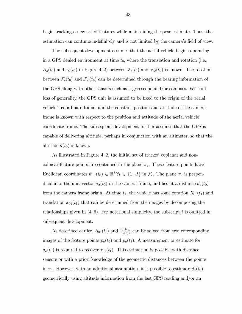
43
begin tracking a new set of features while maintaining the pose estimate. Thus, the
estimation can continue indefinitely and is not limited by the camera’s field of view.
The subsequent development assumes that the aerial vehicle begins operating
in a GPS denied environment at time t0, where the translation and rotation (i.e.,
Ro(t0) and x0(t0) in Figure 4—2) between Fc(t0) and Fw(t0) is known. The rotation
between Fc(t0) and Fw(t0) can be determined through the bearing information of
the GPS along with other sensors such as a gyroscope and/or compass. Without
loss of generality, the GPS unit is assumed to be fixed to the origin of the aerial
vehicle’s coordinate frame, and the constant position and attitude of the camera
frame is known with respect to the position and attitude of the aerial vehicle
coordinate frame. The subsequent development further assumes that the GPS is
capable of delivering altitude, perhaps in conjunction with an altimeter, so that the
altitude a(t0) is known.
As illustrated in Figure 4—2, the initial set of tracked coplanar and non-
colinear feature points are contained in the plane πa. These feature points have
Euclidean coordinates mai(t0) ∈ R3 ∀i ∈ 1...I in Fc. The plane πa is perpen-
dicular to the unit vector na(t0) in the camera frame, and lies at a distance da(t0)
from the camera frame origin. At time t1, the vehicle has some rotation R01(t1) and
translation x01(t1) that can be determined from the images by decomposing the
relationships given in (4—6). For notational simplicity, the subscript i is omitted in
subsequent development.
As described earlier, R01(t1) andx01(t1)da(t0)
can be solved from two corresponding
images of the feature points pa(t0) and pa(t1). A measurement or estimate for
da(t0) is required to recover x01(t1). This estimation is possible with distance
sensors or with a priori knowledge of the geometric distances between the points
in πa. However, with an additional assumption, it is possible to estimate da(t0)
geometrically using altitude information from the last GPS reading and/or an

44
Figure 4—2: Illustration of pose estimation chaining.
altimeter. From the illustration in Figure 4—3, if a(t0) is the height above πa (e.g.,
the slope of the ground is constant between the feature points and projection of the
plane’s location to the ground), then the distance da(t0) can be determined as
da(t0) = na(t0) · a(t0). (4—7)
where na(t0) is known from the homography decomposition.
Once R01(t1), da(t0), and x01(t1) have been determined, the rotation R1(t1)
and translation x1(t1) can be determined with respect to Fw as
R1 = R0R01
x1 = R01x01 + x0.
As illustrated in Figure 4—2, a new collection of feature points pb(t) can be obtained
that correspond to a collection of points on a planar patch denoted by πb. At time
t2, the sets of points pb(t1) and pb(t2) can be used to determine R12(t2) andx12(t2)db(t1)
,
which provides the rotation and scaled translation of Fc with respect to Fw. If πb

45
Figure 4—3: Depth estimation from altitude.
and πa are the same plane, then db(t1) can be determined as
db(t1) = da(t1) = da(t0) + x01(t1) · n(t0). (4—8)
When πb and πa are the same plane x12(t2) can be correctly scaled, and R2(t2) and
x2(t2) can be computed in a similar manner as described for R1(t1) and x1(t1).
Estimations can be propagated by chaining them together at each time instance
without further use of GPS.
In the general case, pb and pa are not coplanar and (4—8) cannot be used to
determine db(t1). If pb and pa are both visible for two or more frames, it is still
possible to calculate db(t) through geometric means. Let t1− denote as some time
before the daisy chain operation is performed, when both pb and pa are visible in
the image. At time t1− , an additional set of homography equations for the points pb
and pa at times t1 and t1−can be solved for

46
mai(t1) = αa
µR+
xna(t1−)T
da(t1−)
¶mai(t1−) (4—9)
mbi(t1) = αb
µR+
xnb(t1−)T
db(t1−)
¶mbi(t1−) (4—10)
where αa =zai(t1− )zai(t)
and αb =zai(t1− )zai(t)
.
Note that R(t1) and x(t1) have the same values in equations (4—9) and (4—
10), but the distance and normal to the plane are different for the two sets of
points. The distance da(t1−) is known from using (4—8). Define xb(t1) =x(t1)
db(t1−)and
xa(t1) =x(t1)
da(t1− ). The translation x(t1) is solved as
x = da(t1−)xa,
and then determining db(t1−)
db(t1−) =xTb x
kxbk.
db(t1) can then be found by using (4—8) with db(t1−) in place of da(t0). Additional
sensors, such as an altimeter, can provide an additional estimate in the change in
altitude. These estimates can be used in conjunction with (4—8) to update depth
estimates.
Image-Based Rate Gyro.
Additional uses are found from the homography decomposition that can be
used for feedback control. As an example, Poisson’s kinematic differential equation
for the direction cosine matrix, R states
R = −
⎡⎢⎢⎢⎢⎣0 −r q
r 0 −p
−q p 0
⎤⎥⎥⎥⎥⎦R,which can also be expressed as

47
⎡⎢⎢⎢⎢⎣0 −r q
r 0 −p
−q p 0
⎤⎥⎥⎥⎥⎦ = −RRT .
Hence, aircraft body rates, p (t) , q (t) ,and r (t) can be estimated via R (t) from the
homography decomposition along with the time derivative of R (t) .
4.2.4 Simulation Results
In the simulations, five patches of 4 feature points are manually placed
along a 500 meter ground track, which the vehicle flies over. For simplicity, all
planar patches lie in the same plane. The task is to perform the state estimation
during a maneuver. The commanded maneuver is to simultaneously perform a 10
meter lateral shift to the right and a 10 meter longitudinal increase in altitude.
This particular maneuver results in the vehicle simultaneously pitching, rolling,
and yawing, while translating. For simulation purposes, the camera is mounted
underneath the fuselage looking downwards. The camera model for this exercise
is intended to be representative of a typical 640×480 lines of resolution CCD
camera equipped with a 10 mm lens. To more accurately capture true system
performance, pixel coordinates were rounded to the nearest integer to model errors
due to camera pixilation effects (i.e. quantization noise), furthermore a 5% error
was added to the estimated vehicle altitude to test robustness.
The first simulation was designed to test the accuracy of the vision-based esti-
mation. Vision was not used in the feedback in this maneuver, and the estimated
pose is compared to the true pose. The results of this preliminary analysis are
given in Figures 4—4 and 4—5. The effects of noise are visible but the estimated pose
is accurate.
The second simulation was intended to examine the effects of using the
vision based estimate as a sensor in closed-loop control. This simulation involved
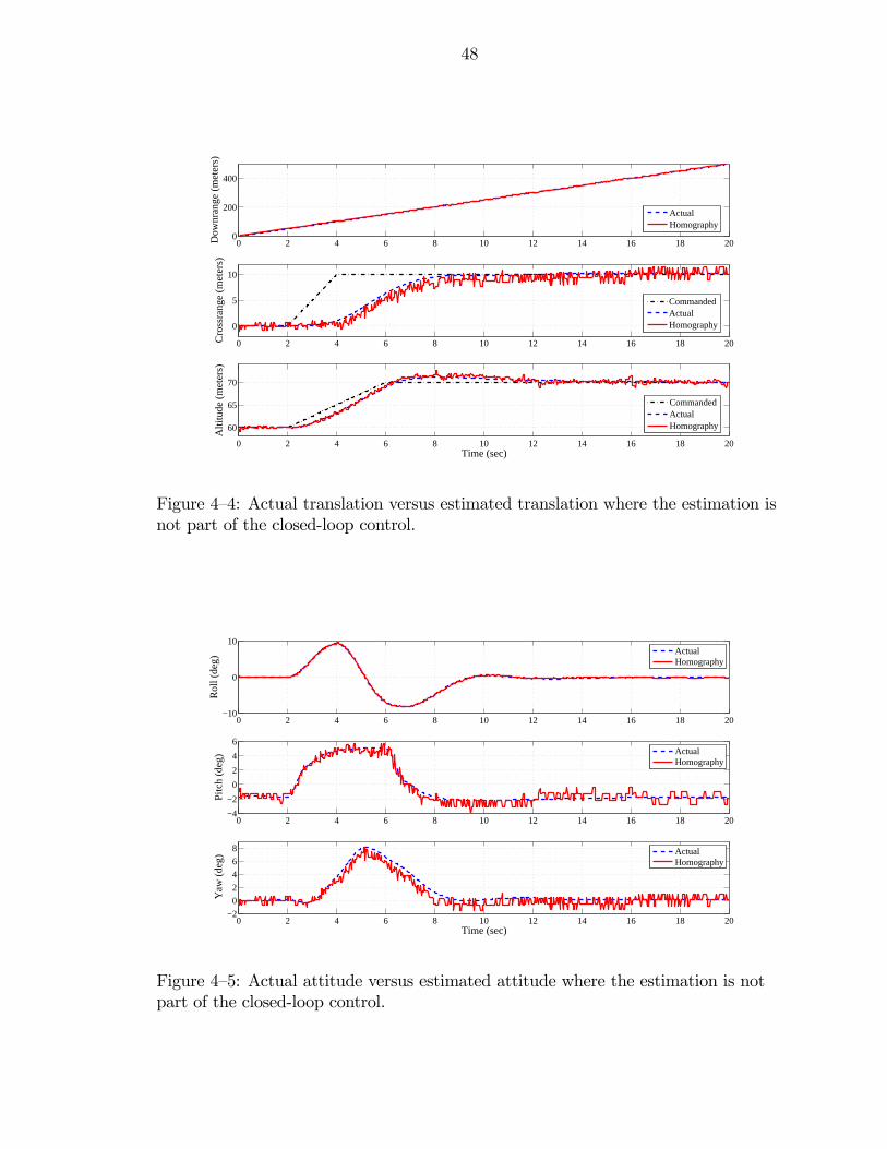
48
0 2 4 6 8 10 12 14 16 18 200
200
400
Dow
nran
ge (
met
ers)
ActualHomography
0 2 4 6 8 10 12 14 16 18 20
0
5
10
Cro
ssra
nge
(met
ers)
CommandedActualHomography
0 2 4 6 8 10 12 14 16 18 20
60
65
70
Time (sec)
Alti
tude
(m
eter
s)
CommandedActualHomography
Figure 4—4: Actual translation versus estimated translation where the estimation isnot part of the closed-loop control.
0 2 4 6 8 10 12 14 16 18 20−10
0
10
Rol
l (de
g)
ActualHomography
0 2 4 6 8 10 12 14 16 18 20−4
−2
0
2
4
6
Pitc
h (d
eg)
ActualHomography
0 2 4 6 8 10 12 14 16 18 20−2
0
2
4
6
8
Time (sec)
Yaw
(de
g)
ActualHomography
Figure 4—5: Actual attitude versus estimated attitude where the estimation is notpart of the closed-loop control.

49
replacing the perfect position and attitude measurements, used in the guidance
system and autopilot, with position and attitude estimations determined from the
vision-based method. The resulting control architecture and sensor suite for this
autonomous air vehicle is given in Figure 4—6. The noise content of the estimated
position and attitude required filtering prior to being used by the autopilot, to
prevent the high frequency noise from being passed to the aircraft actuators. As
expected, the noise occurs at 30 Hz and corresponds to the frame rate of the
camera. First-order, low pass-filters (cutoff frequency as low as 4 rad/sec) were
used to filter the noise. The noise also prevented effective differentiation of the
position and attitude and necessitated the use of rate gyros for yaw and roll
damping, as depicted in Figure 4—6. The air data system is also included, as shown
in Figure 4—6, for the initial altitude measurement, since it is more accurate for
altitude than current GPS solutions. The results of the camera-in-the-loop system
performing the same guidance commanded autonomous maneuver are given in
Figures 4—7 and 4—8.
The simulation results indicate that a camera supplemented with minimal
sensors such as rate gyros and barometric altitude can be used for completely
autonomous flight of a fixed wing vehicle; however, some residual oscillation effects
due to noise is present in the vehicle attitude response. A majority of the noise
source can directly be attributed to camera pixilation effects and the corresponding
phase lag introduced by the first order filtering.
4.2.5 Experimental Results
Based on the results of the simulation, a flight test experiment was conducted
to establish the feasibility of the proposed vision-based state estimation method.
Artificial features were placed along a stretch of the runway. A radio controlled
aircraft with an onboard camera was flown over the runway. The video was overlaid
with GPS data from a Garmin GPS 35 receiver. An example of a single frame of
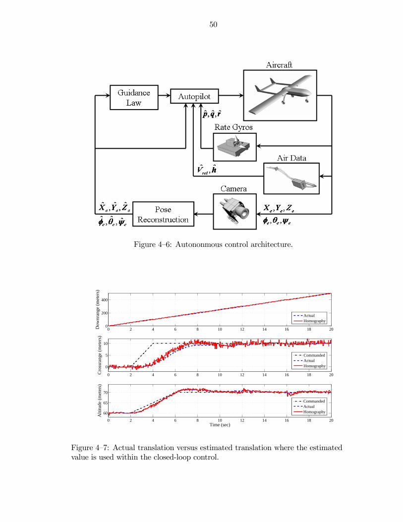
50
Figure 4—6: Autononmous control architecture.
0 2 4 6 8 10 12 14 16 18 200
200
400
Dow
nran
ge (
met
ers)
ActualHomography
0 2 4 6 8 10 12 14 16 18 20
0
5
10
Cro
ssra
nge
(met
ers)
CommandedActualHomography
0 2 4 6 8 10 12 14 16 18 20
60
65
70
Time (sec)
Alti
tude
(m
eter
s)
CommandedActualHomography
Figure 4—7: Actual translation versus estimated translation where the estimatedvalue is used within the closed-loop control.

51
0 2 4 6 8 10 12 14 16 18 20−10
0
10
Rol
l (de
g)
ActualHomography
0 2 4 6 8 10 12 14 16 18 20−4−2
02468
Pitc
h (d
eg)
ActualHomography
0 2 4 6 8 10 12 14 16 18 20
0
5
10
Time (sec)
Yaw
(de
g)
ActualHomography
Figure 4—8: Actual attitude versus estimated attitude where the estimated value isused within the closed-loop control.
this video is given in Figure 4—10. A second GPS unit (manufactured by Eagle
Tree Systems, LLC) was also onboard to test inter-GPS accuracy. The use of two
GPS units provides comparison for the vision-based method, which is intended to
compute GPS-like information. Video data was captured using a DV tape recorder
and analyzed offline. A basic descriptive pictorial of what equipment was used
(minus the eagle tree system) and the corresponding signal flow is given in Figure
4—9. See the Appendix for a more detailed description of the ground and airborne
equipment. Due to poor image quality, including focus, motion blur and interlacing
of the DV video, it became necessary to extract features by hand from individual
frames. Features were extracted every sixth frame, resulting in a 5 Hz input signal.
Results of the experiment are given in Figure 4—11. In the legend for Figure
4—11, GPS2 represents the overlaid GPS data, and GPS1 represents the onboard
data logger GPS values. A ‘*’ in the plot indicates a time when daisy-chaining was
performed and pose reconstruction is performed using a new set of feature points.

52
Figure 4—9: Overview of the flight test system and component interconnections.
Figure 4—10: Single video frame with GPS overlay illustrating landmarks placedalong inside edge of the runway.

53
0 2 4 6 8 10 12 14 16 18 20 220
200
400
600
Dow
nran
ge (
m)
HomographyGPS1GPS2
0 2 4 6 8 10 12 14 16 18 20 22
−50
0
50
100
Cro
ssra
nge
(m)
HomographyGPS1GPS2
0 2 4 6 8 10 12 14 16 18 20 22
0
50
100
Time (sec)
Alti
tude
(m
)
− represents where daisy−chain occurs
HomographyGPS1GPS2
*
Figure 4—11: Experimental flight test results. Estimated position compared to twoGPS signals.
The results from this test appear to be very promising. Significant mismatch exists
between the two GPS measurements, and the vision-based estimation remains
proportionate to the two GPS measurements. Furthermore, the estimates agree
closely with GPS2 for downrange and crossrange translation, and with GPS1 for
altitude translation. There is no discernible discontinuity or increased error at the
daisy-chain handoff times. Note that the resolution of the vision-based estimation
(5Hz) is also higher than that of both GPS units (1Hz). The pose estimation code
can be executed in real time (>30Hz) on a typical laptop.
The accuracy of the GPS data, as recorded, is arguably dubious, therefore
an alternate flight test was designed that was intended to enable the vehicle
position to be determined with greater accuracy than what could be achieved with
the inexpensive GPS units used in the first round of testing. In addition to the
issues with the GPS output being used as "truth data", it was also of interest
to investigate whether using a wider angle field of view lens on a more forward

54
Figure 4—12: Technique for achieving accurate landmark relative placement dis-tances.
pointing camera could improve the results. The fundamental assumption of this
additional testing was that if the locations of the ground targets were known
precisely, then the position of the vehicle could be ascertained more accurately
through geometric reconstruction than what could be achieved with low cost GPS
units.
Similar to before, plates/landmarks were placed along 274.32 meters (900 feet)
of the runway. Unlike before, they were placed at 15.24 meter (50 foot) intervals
where the accuracy of each plate location was known to within a few inches along
the entirety of the 274.32 meters (900 feet) span. The two rows of plates, left and
right of the runway centerline, were 18.59 meters (61 feet) apart. The plates were
painted red so that a simplistic feature tracking algorithm could be used to locate
and track their location in the image plane. The equipment that was used for
surveying the landmarks is shown in Figure 4—12.
By using a wider field of view lens, the resulting video image exhibited severe
lens distortion effects that required correcting in order for the homography to

55
Figure 4—13: Single video frame from second flight test experiment illustrating theeffect of the more forward looking, wider field of view camera.
operate correctly. The distortion can be seen in Figure 4—13, where the four red
landmarks in the lower portion of the frame appear to be located on a spherical
surface as opposed to a plane; again, a fundamental requirement in the develop-
ment of the homography method. This same image with the distortion removed
is given in Figure 4—14. The interlacing effect, prevalent in Figure 4—10 has also
been removed. As mentioned, the features were tracked and their trajectories in the
image plane recorded using a simplistic ad-hoc scheme in Matlab. The pseudocode
for tracking the four features of a single patch is given as:
Manually determine the location to initialize a 40x40 pixel window over each of the
four landmarks in the first image
FOR all images containing the same patch of four landmarks
Read the next image in the sequence and assign it to an RGB color space array
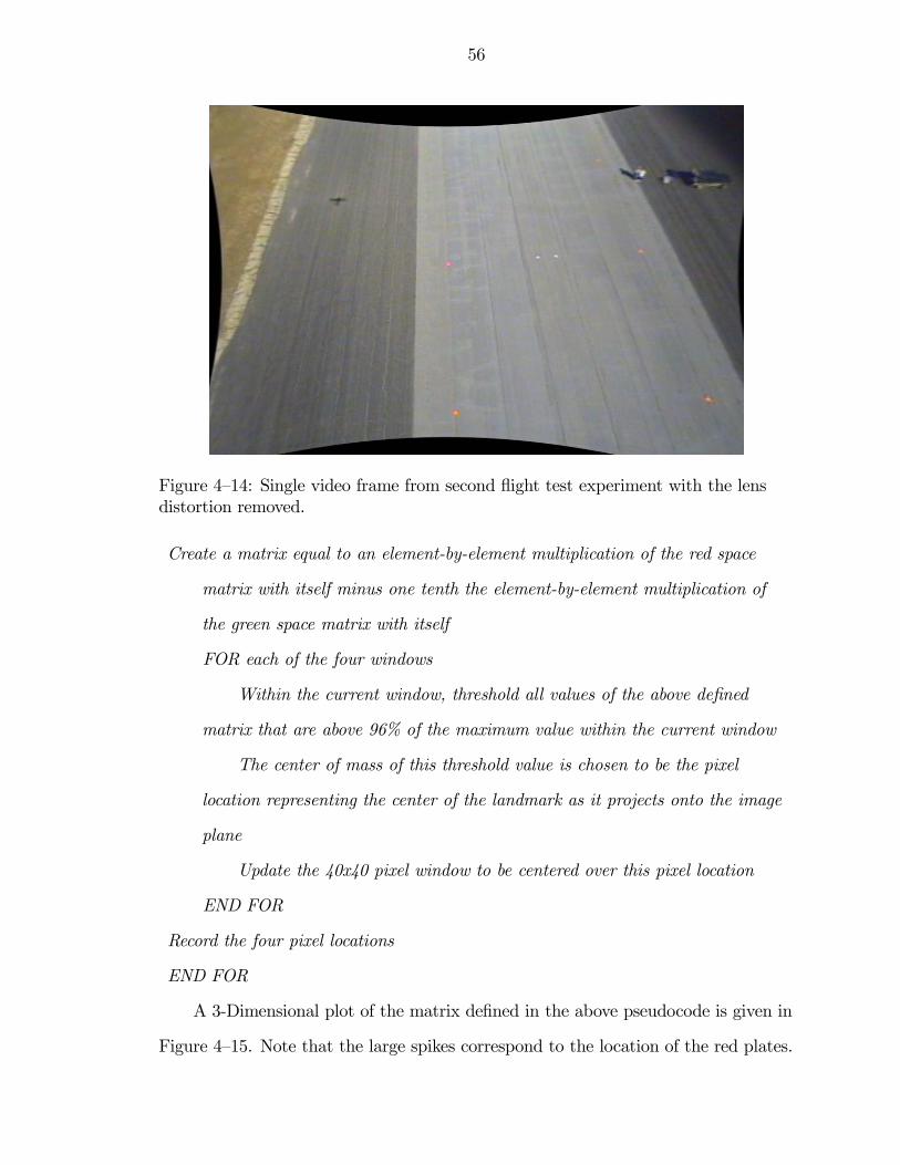
56
Figure 4—14: Single video frame from second flight test experiment with the lensdistortion removed.
Create a matrix equal to an element-by-element multiplication of the red space
matrix with itself minus one tenth the element-by-element multiplication of
the green space matrix with itself
FOR each of the four windows
Within the current window, threshold all values of the above defined
matrix that are above 96% of the maximum value within the current window
The center of mass of this threshold value is chosen to be the pixel
location representing the center of the landmark as it projects onto the image
plane
Update the 40x40 pixel window to be centered over this pixel location
END FOR
Record the four pixel locations
END FOR
A 3-Dimensional plot of the matrix defined in the above pseudocode is given in
Figure 4—15. Note that the large spikes correspond to the location of the red plates.

57
Figure 4—15: Example of a 3D color contour plot generated from the matrix de-signed as a nonlinear combination of the red and green color space matrices.
Values that are above 96% of the maximum value of each spike are thresholded and
the centers-of-mass of these thresholded values are used to determine the predicted
centers of the landmarks in the image frame. By following this procedure, it was
predicted that sub-pixel accuracy could be achieved over simply selecting the pixel
location of the maximum value or tip of the spike.
An example of the output of the above tracking algorithm is also given in
Figure 4—16. The four trajectories in this particular case represent the trace of the
landmarks from the first patch as it enters and exits the field of view (from top to
bottom). As a point of interest, note that the center of the image plane does not
correspond to location of the optical axis. This apparent oddity is in keeping with
the camera calibration results and is most likely congruous with a low end imager
and lens.
With the trajectories of the four landmarks of each patch recorded, vehicle lo-
calization can then be performed offline for analysis purposes. It should be pointed

58
−200
−100
0
100
200
300−400 −300 −200 −100 0 100 200 300 400 500
Ver
tical
Pix
el L
ocat
ion
Horizontal Pixel Location
x
y
Figure 4—16: Image plane trajectories made by the landmarks from patch 1 enter-ring and exiting the field of view.
out that the 40 × 40 pixel window is designed such that it is large enough to con-
tain the landmark in the current frame and the subsequent frame. Smaller windows
tended to not encapsulate both the current and subsequent frame landmarks due to
vehicle motions between frames.
For a given set of three feature points, and knowledge of where those land-
marks are in the earth frame, geometric reconstruction can be used to back out the
location of the aircraft. This is illustrated in Figure 4—17, where in this particular
illustration, a tetrahedron is used to determine the x0, y0, and z0 location of the
camera in the earth frame. e1, e2, and e3 are known a priori relative distances
between the 3 landmarks. Vertex angles η1, η2, and η3 of the apex of the tetrahe-
dron are determined by the focal length of the camera lens in pixel coordinates in
conjunction with the pixel locations of where the landmarks corresponding to line
segments e1, e2, and e12 occur in the image plane. The value for the skew, χ is used
to account for the fact that the four landmarks most likely form a parallelogram,

59
since it was somewhat difficult to create a perfect rectangle in the field. In fact, e12
depends upon the skew, χ and is calculated according to
e12 =qe21 sec
2 (χ) + e22 + 2e1e2 sec (χ) sin (χ)
Presuming a, b, and c can be computed, then x0, y0, and z0 of the camera can
be determined via the following series of calculations:
ϕ1 = cos−1µe212 + c2 − a2
2e12c
ϕ2 = cos−1µe212 + e22 − e212e12e2
¶and a0, shown in Figure 4—17, is calculated from the following
a0 =qe22 sec
2 (ϕ2) + c2 − 2ce2 cos (ϕ1) |sec (ϕ2)|
If b is considered as a vector, the x and y direction cosines are given by, respec-
tively
cosσ1 =e22 + b2 − c2
2e2b
cosσ2 =e22 tan
2 (ϕ2) + b2 − a02
2e2 tan (ϕ2) b
Finally, the components of the position vector from the origin of the earth frame to
the origin of the camera frame, in earth frame coordinates, is simply
x0 = b cos (σ1)
y0 = b cos (σ2)
z0 = bqsin2 (σ1)− cos2 (σ2)
The difficulty of this method for pose estimation is in determining a, b, and c,
more specifically, the edge lengths of the tetrahedron in Figure 4—17. The reason
is that for given values of η1, η2, and η3 and e1, e2, and e12, there can be as little
as zero physically possible solutions and as many as three distinctly different

60
Figure 4—17: Basic concept of geometric position reconstruction from known land-mark locations.
physically possible tetrahedrons. The possible values of a, b, and c are determined
by simultaneously solving the three law-of-cosine rules for the three triangular
facets making up the upright sides of the tetrahedron. A forth landmark is needed
to resolve the correct a, b, and c, via constructing multiple tetrahedrons, clocking
around the four landmarks as shown in Figure 4—18, and selecting the a, b, c, and
d that are common to all four tetrahedrons. Using this technique, each edge length
is calculated three times. A merit of how reliable or accurate our position estimate
is, and hence, how well the proper pixels representing the landmark centers were
selected, is in how close each of the three edge length calculations a, b, c, and d
are to each other. A quick convincing argument would be in the event that a, b,
c, and d are the exact same in all 3 calculations, one could be very certain that
they would consistently project and reproject back and forth between the camera
and a surface containing 4 points with the same edge lengths e1, e2, e3, and e4.

61
Figure 4—18: Illustration of how four tetrahedrons are used to estimate the lengthof each edge, a, b, c, & d three times.
If this surface can be shown to be a plane, then intuitively, this plane and four
points would, with high confidence, be the earth plane and the points would be the
centers of the landmarks. Results of this flight experiment are given in Figure 4—19.
Because time was not recorded for this experiment, the ground track trajectory is
given as opposed to downrange and crossrange time responses as given in Figure
4—11. The color variation in the geometric reconstruction represent the individual
patches used along the length of the runway. The origin of the earth frame is
placed at the first plate on the lower right that appears when the vision estimation
begins. Also noteworthy, because this experiment used a somewhat forward looking
camera, the camera position starts in the negative x-direction because the first
plate is ahead of the camera; conversely, the camera is behind the first plate.
4.3 Conclusions
The efforts in this chapter integrated new vision-based pose estimation
methods with the flight controls of an aerial vehicle in a guidance task. This
method is based on Epipolar geometry, with a novel “daisy-chaining” approach

62
−50 0 50 100 150 200 2500
5
10
15
20
X − Distance Down Runway (m)
Y −
Dis
tanc
e A
cros
s R
unw
ay (
m)
Geometric Reconstruction
Homography
Figure 4—19: Second experimental flight test results. Estimated position comparedto more accurate position from geometric reconstruction technique.
allowing image features to enter and leave the field of view while maintaining pose
estimation. Furthermore, no known target is required.
The vision-based pose estimation method was verified experimentally with
a radio controlled Osprey aircraft. Because the accuracy of the onboard GPS
measurements was considered questionable, an alternate effort involving geometric
reconstruction for position determination was undertaken to better represent truth
data for validating the daisy-chaining pose estimation technique. To facilitate the
experiments, a nonlinear aircraft flight model for the Osprey was developed to
allow extensive simulation testing. Simulations include testing the pose estimation
method in closed-loop control of the aircraft through an intentionally rigorous
maneuver to evaluate the robustness of the technique.
The ultimate goal of this research is closed-loop control using camera data
in place of GPS. To this end, future research will target online feature extraction,
tracking, and pose estimation. Furthermore, a future task would be to investigate
the use of nonlinear control techniques, such as discussed in the next chapter, to
eliminate or reduce the amount of required a priori known information required
in the estimation strategy. Additional sensor data such as IMU’s and intermit-
tent GPS could also be fused with the vision-based pose estimation to enhance
performance.

CHAPTER 5LYAPUNOV-BASED STATE ESTIMATION
5.1 Introduction
Many applications require the interpretation of the Euclidean coordinates of
features of a 3-dimensional (3D) object through 2D images. In this chapter, the
relative range and the Euclidean coordinates of a camera undergoing general affine
motion are determined for pinhole camera systems via a nonlinear observer. The
nonlinear observer asymptotically determines the range information provided that
the motion parameters are known. The observer is developed through a Lyapunov-
based design and stability analysis, and simulation results are provided that
illustrate the performance of the state estimator. The contributions of this chapter
are that the developed observer: can be applied to both affine and nonaffine
systems; is continuous; and yields an asymptotic result.
5.2 Affine Euclidean Motion
For the development in this dissertation, the scenario of a moving camera
viewing a static scene to recover the structure of the scene and/or the motion of
the camera (cf., [53, 84, 85], and therein) is considered. The affine motion of the
camera dynamics can be expressed as⎡⎢⎢⎢⎢⎣x1
x2
x3
⎤⎥⎥⎥⎥⎦ =⎡⎢⎢⎢⎢⎣
a11 a12 a13
a21 a22 a23
a31 a32 a33
⎤⎥⎥⎥⎥⎦⎡⎢⎢⎢⎢⎣
x1
x2
x3
⎤⎥⎥⎥⎥⎦+⎡⎢⎢⎢⎢⎣
b1
b2
b3
⎤⎥⎥⎥⎥⎦ (5—1)
where x(t) = [x1(t), x2(t), x3(t)]T ∈ R3 denotes the unmeasurable Euclidean
coordinates of the moving camera along the X, Y , and Z axes of a camera fixed
reference frame, respectively, where the Z axis is colinear with the optical axis
63

64
of the camera. In (5—1), the parameters ai,j(t) ∈ R ∀i, j = 1, 2, 3 of the matrix
A(t) ∈ R3×3 and b(t) = [b1, b2, b3]T ∈ R3 denote the motion parameters. The affine
motion dynamics introduced in (5—1) are expressed in a general form that describes
an object motion consisting of a rotation, translation, and linear deformation [86].
Assumption 5.1: The motion parameters in A(t) and b(t) introduced in
(5—1) are assumed to be known, bounded functions of time that are second order
differentiable.(cf. [51,55—60,87—89]).
To illustrate how the affine dynamics in (5—1) represent a moving camera
viewing a stationary object (see Figure 5—1), consider a feature point attached
to a stationary object as in Figure 5—1. In Figure 5—1, Fc denotes a body-fixed
coordinate frame attached to the camera, I denotes an inertial coordinate frame
and x(t) (expressed in Fc) denotes the coordinates of the target feature point Oi.
The linear and angular velocities of the target (i.e., vt(t) and ωt(t)) with respect to
the camera (expressed in Fc) can be written as
vt = −Rvc ωt = −Rωc (5—2)
where R(t) ∈ R3×3 denotes the corresponding rotation between Fc and I, and vc(t)
and ωc(t) denote the linear and angular velocity of the camera, respectively. Based
on (5—2), The time derivative of x(t) can be expressed as
x = [Rωc]× x+Rvc = Ax+ b. (5—3)
Potential applications for this scenario under the restriction of Assumption 1
include examples where the camera is moving with a known/measurable linear
and angular velocity where the goal is to estimate the Euclidean position of the
moving camera in time, such as: inertial navigation in GPS denied environments
and simultaneous localization and mapping (SLAM).

65
oi
moving camera
cF
X
Yc
Zc
fixed target
1(x , x , x )2 3=x T
Ic
Figure 5—1: Moving camera stationary object scenario.
Figure 5—2: Euclidean point projected onto image plane of a pinhole camera

66
5.3 Object Projection
The projection of the coordinates x(t) onto an image plane with its focus at
the origin (see Figure 5—2) can be expressed as
p (t) ,∙u v
¸T=
f
z
∙x y
¸T(5—4)
where f ∈ R denotes the constant known distance between the focal point and the
image plane.
Deriving the expression for the time rate of change of pixel location by taking
the time derivative of (5—4) and utilizing (5—1) as
p (t) = Ω1 + g, (5—5)
where Ω1(u, v, t) ∈ R2 denotes a vector of measurable and known signals defined by
Ω1(t) ,
⎡⎢⎣ a11 a12 a13
a21 a22 a23
⎤⎥⎦⎡⎢⎢⎢⎢⎣
u
v
f
⎤⎥⎥⎥⎥⎦− 1f⎡⎢⎣ u
v
⎤⎥⎦∙ a31 a32 a33
¸⎡⎢⎢⎢⎢⎣u
v
f
⎤⎥⎥⎥⎥⎦ (5—6)
and the unmeasurable signal g(t) , [g1(t), g2(t)] ∈ R2 is defined as
g(t) ,
⎧⎪⎨⎪⎩f
⎡⎢⎣ b1
b2
⎤⎥⎦−⎡⎢⎣ u
v
⎤⎥⎦ b3⎫⎪⎬⎪⎭ 1
z. (5—7)
From the above definition for g(t), the following expression can be written:
g21 + g22 =
½(fb1 − ub3)
1
z
¾2+
½(fb2 − vb3)
1
z
¾2(5—8)
=£(fb1 − ub3)
2 + (fb2 − vb3)2¤½1
z
¾2.
Based upon (5—8) the time varying depth estimation can be expressed as,

67
z =
s(fb1 − ub3)
2 + (fb2 − vb3)2
g21 + g22(5—9)
Assumption 5.2: The image-space feature coordinates u(t), v(t) are bounded
functions of time.
Assumption 5.3: If g(t) can be identified, then z(t) can be determined
from (5—7), provided b1, b2, b3 6= 0 simultaneously. This observability assumption
physically means that the object must translate in at least one direction.
Remark 5.1: Based on Assumptions 5.1-5.3, the expressions given in (5—5)-
(5—9) can be used to determine that p(t), Ω1(t), and g(t) ∈ L∞. Given that these
signals are bounded, Assumptions 5.1-5.3 can be used to prove that
kg(·)k ≤ ζ1 kg(·)k ≤ ζ2 kg(·)k ≤ ζ3 (5—10)
where ζ1, ζ2 and ζ3 ∈ R denote known positive constants.
5.4 Range Identification For Affine Systems
5.4.1 Objective
The objective of this section is to extract the Euclidean coordinate information
of the object feature from its image-based projection. From (5—4) and the fact
that u(t), and v(t) are measurable, if z(t) could be identified, then the complete
Euclidean coordinates of the feature can be determined. To achieve this objective,
an estimator is constructed based on the unmeasurable image-space dynamics
for p(t). To quantify the objective, a measurable estimation error, denoted by
e(t) , [e1(t), e2(t)]T ∈ R2, is defined as follows:
e = p− p (5—11)
68
where p(t) , [p1(t), p2(t)]T ∈ R2 denotes a subsequently designed estimate. An
unmeasurable1 filtered estimation error, denoted by r(t) , [e1(t), e2(t)]T ∈ R2, is
also defined as
r = e+ αe (5—12)
where α ∈ R2×2 denotes a diagonal matrix of positive constant gains α1, α2 ∈ R.
Motivation for the development of the filtered estimation error in (5—12), is that
the subsequent observer is based on the equation (5—5). If g(t) in (5—5) can be
identified, the fact that the feature point coordinates pi(t) ∀i = 1, 2 are measurable
can be used along with (5—9) to compute z(t) provided the observability condition
in Assumption 5.3 is satisfied.
5.4.2 Estimator Design and Error System
Based on (5—5) and the subsequent analysis, the following estimation signals
are defined:
˙p (t) = Ω1 + g (5—13)
where g(t) , [g1(t), g2(t)]T ∈ R2 denotes a subsequently designed estimate for g(t).
The following error dynamics are obtained after taking the time derivative of e(t)
and utilizing (5—5) and (5—13):
e = g − g. (5—14)
Based on the structure of (5—12) and (5—14),·g(t) is designed as follows [56]:
·g = −(ks + α)g + γsgn(e) + αkse (5—15)
where ks, γ ∈ R3×3 denote diagonal matrices of positive constant estimation gains,
and the notation sgn(·) is used to indicate a vector with the standard signum
1 The filtered estimation signal is unmeasurable due to a dependence on the un-measurable terms g1(t), g2(t).

69
function applied to each element of the argument. The structure of the estimator
in (5—15) contains discontinuous terms; however, as discussed in [56], the overall
structure of the estimator is continuous (i.e., g(t) is continuous). After using
(5—12), (5—14), and (5—15), the following expression can be obtained:
r = η − ksr − γsgn(e) (5—16)
where η(t) ,∙η1 η2
¸T∈ R2 is defined as
η = g + (ks + α) g. (5—17)
Based on (5—10) and (5—17), the following inequalities can be developed:
|η(·)| ≤ ζ4 |η(·)| ≤ ζ5. (5—18)
where ζ4 and ζ5 ∈ R denote known positive constants.
Remark 5.1: Considering (5—9), the unmeasurable signal z(t) can be identi-
fied if g(t) approaches g(t) as t → ∞ (i.e., u(t) and v(t) approach u(t) and v(t) as
t→∞) since the parameters bi(t) ∀i = 1, 2 are assumed to be known, and u(t) and
v(t) are measurable. After z(t) is identified, (5—4) can be used to extract the 3D
Euclidean coordinates of the object feature (i.e. determine the range information).
To prove that g(t) approaches g(t) as t → ∞, the subsequent development will
focus on proving that ke(t)k → 0 and ke(t)k → 0 as t → ∞ based on (5—11) and
(5—14).
5.5 Analysis
The following theorem and associated proof can be used to conclude that the
observer design of (5—13) and (5—15) can be used to identify the unmeasurable
signal z(t).
Theorem 5.1: For the system in (5—5)-(5—7), the unmeasurable signal z(t)
(and hence, the Euclidean coordinates of the object feature) can be asymptotically

70
determined from the estimator in (5—13) and (5—15) provided the elements of the
constant diagonal matrix γ introduced in (5—15) are selected according to the
sufficient condition
γi ≥ ζ4 +1
αiζ5 (5—19)
∀i = 1, 2, where ζ4, ζ5 are defined in (5—18).
Proof: Consider a non-negative function V (t) ∈ R as follows (i.e., a Lyapunov
function candidate):
V =1
2rT r . (5—20)
After taking the time derivative of (5—20) and substituting for the error system
dynamics given in (5—16), the following expression can be obtained:
V = −rTksr + (e+ αe)T (η − γsgn(e)) . (5—21)
After integrating (5—21) and exploiting the fact that
ξi · sgn(ξi) = |ξi| ∀ξi ∈ R,
the following inequality can be obtained:
V (t) ≤ V (t0)−Z t
t0
¡rT (σ) ksr (σ)
¢dσ+
2Xi=1
αi
Z t
t0
|ei (σ)| (|ηi (σ)|− γi) dσ+χi, (5—22)
where the auxiliary terms χi(t) ∈ R are defined as
χi =
Z t
t0
ei (σ) ηi (σ) dσ − γi
Z t
t0
ei (σ) sgn(ei (σ))dσ (5—23)
∀i = 1, 2. The integral expression in (5—23) can be evaluated as
χi = ei (σ) ηi (σ)|tt0 −Z t
t0
ei (σ) ηi (σ) dσ − γi |ei (σ)| |tt0 (5—24)
= ei (t) ηi (t)−Z t
t0
ei (σ) ηi (σ) dσ − γi |ei (t)|− ei (t0) ηi (t0) + γi |ei (t0)|

71
∀i = 1, 2. Substituting (5—24) into (5—22) and performing some algebraic manipula-
tion yields
V (t) ≤ V (t0)−Z t
t0
¡rT (σ) ksr (σ)
¢dσ + χ3 + ζ0
where the auxiliary terms χ3(t), ζ0 ∈ R are defined as
χ3 =2X
i=1
αi
Z t
t0
|ei (σ)|µ|ηi (σ)|+
1
αi|ηi (σ)|− γi
¶dσ +
2Xi=1
|ei (t)| (|ηi (t)|− γi)
ζ0 =2X
i=1
− ei (t0) ηi (t0) + γi |ei (t0)| .
Provided γi ∀i = 1, 2 are selected according to the inequality introduced in (5—19),
χ4(t) will always be negative or zero; hence, V (t) can be upper bounded as
V (t) ≤ V (t0)−Z t
t0
¡rT (σ) ksr (σ)
¢dσ + ζ0 . (5—25)
From (5—20) and (5—25), the following inequalities can be determined:
V (t0) + ζ0 ≥ V (t) ≥ 0;
hence, r(t) ∈ L∞. The expression in (5—25) can be used to determine thatZ t
t0
¡rT (σ) ksr (σ)
¢dσ ≤ V (t0) + ζ0 <∞ . (5—26)
By definition, (5—26) can now be used to prove that r(t) ∈ L2. From the fact
that r(t) ∈ L∞, (5—11) and (5—12) can be used to prove that e(t), e(t), p(t), and·p(t) ∈ L∞. The expressions in (5—13) and (5—15) can be used to determine that
g(t) and·g(t) ∈ L∞. Based on (5—10), the expressions in (5—16) and (5—17) can be
used to prove that η(t), η(t), r(t) ∈ L∞. Based on the fact that r(t), r(t) ∈ L∞
and that r(t) ∈ L2, Barbalat’s Lemma [90] can be used to prove that kr(t)k → 0
as t → ∞; hence, standard linear analysis can be used to prove that ke(t)k → 0
and ke(t)k → 0 as t → ∞. Based on the fact that ke(t)k → 0 and ke(t)k → 0
as t → ∞, the expression given in (5—11) can be used to determine that p1(t) and

72
p3(t) approach p1(t) and p3(t) as t → ∞, respectively. Therefore, the expression in
(5—14) can be used to determine that g(t) approaches g(x) as t → ∞. The result
that g(t) approaches g(t) as t → ∞, the fact that the parameters bi(t) ∀i = 1, 2, 3
are assumed to be known, and the fact that the image-space signals p1(t) and p3(t)
are measurable can be used to identify the unknown signal z(t) from (5—9). Once
z(t) is identified, the complete Euclidean coordinates of the object feature can be
determined using (5—4).
With the Euclidean coordinates of the object known, a simplistic method
for determining aircraft altitude above the ground could employ the following
relationship:
h = x sinφ cos θ + y cosφ cos θ cos ρ+ sin θ sin ρ+ z cosφ cos θ sin ρ− sin θ cos ρ
where ρ is the downward look angle of the camera with respect to the aircraft and
φ and θ represent the aircraft roll and pitch angle respectively.
5.6 Conclusion
The results in this chapter focus on the use of a nonlinear estimator to deter-
mine the range and the Euclidean coordinates of an object feature with respect the
camera coordinate system undergoing general affine motion. The nonlinear esti-
mator is proven, via a Lyapunov-based analysis, to asymptotically determine the
range information for a camera system with known motion parameters. If specific
observability conditions are satisfied, the identified range can be used to reconstruct
the Euclidean coordinates of the moving aircraft with respect to a fixed object on
the ground .

CHAPTER 6CONTRIBUTIONS AND FUTURE WORK
A novel vision-based estimation, localization, and control methodology is
presented for enabling autonomous flight of a fixed-wing air vehicle; providing
it with the capability of flying indefinitely over a region composed of planar
patches of feature points. The proposed daisy-chaining approach is distinct from
the majority of the current vision-based methods of state estimation in that
current methods usually require some degree of a priori knowledge of landmarks
or are specifically designed for hovering vehicles and therefore are not devised to
handle feature points entering and leaving the field-of-view of the camera. One
contribution of this dissertation is that it is the first occasion that a homography-
based state estimation method is presented to handle feature points entering and
leaving the camera field-of-view. As a result, this is also the first time in which
a camera has been demonstrated to act as the sole sensor, with the exception of
an altimeter for approximating height above a given planar patch, for estimating
aircraft position during flight into a GPS denied environment. As a compliment to
these results and to address the requirement for an estimation of the height above
a given planar patch, a Lyapunov-based state estimator, used in combination with
the daisy-chaining method, is the first instance of illustrating the plausibility of
autonomous air vehicle flight over an indefinite distance with the camera “truly”
acting as the sole vehicle sensor.
Using a video camera as the primary sensor in aircraft control requires special
consideration from a controls standpoint. In addition to such presented concerns,
as the air vehicle is required to fly in lesser benign regimes, such as with agile
maneuvering, it becomes evident that simplistic classical control methods will be
73

74
limited in capability and performance. Therefore, in order to fly an aircraft in a
closed-loop sense using a camera as a primary sensor, the controller needs to be
robust to not only parametric uncertainties, but to system noise that is of the
kind uniquely characteristic of camera systems. A novel nonlinear controller is
presented as a credible answer to such anticipated issues, resulting in the first case
of developing an aircraft controller for an uncertain system that provides a semi-
global asymptotically stable result, where there exists input uncertainty as well as
generalized additive nonlinear disturbances that are state and time varying. Future
work on this control approach should attempt to eliminate the requirement that
the filtered tracking error needs to be measured, as opposed to the more desirable
situation of simply measuring the tracking error.
Other possible future work that builds upon what is presented in this dis-
sertation would be to investigate methods that would allow the relaxation of the
coplanar requirement, i.e. navigation over a non-flat earth, to fuse the homography-
based daisy-chain estimates with additional sensors for improved accuracy, and
to perform a comparison analysis by applying estimation methods (i.e. Kalman
filtering) to both feature point tracking in the image plane as well as vehicle state
estimation. Potential future work might also be to investigate multiple vehicles
for use in the homography-based daisy-chaining method as an analogue to what is
currently being researched within the field of cooperative-SLAM.
Because error from the homography-based daisy-chain estimate accumulates
with each handoff, it would also be of interest to perform flight experiments that
combine the Lyapunov-based state estimator with the daisy-chaining method.
In doing so, one could investigate using an updated height above planar patch
measurement between each hand-off to reduce the effect of accumulating position
error. This improvement would be expected since position error scales with the
error in the estimated magnitude of the vector that is defined by being both normal

75
to the planar patch and extending from the planar patch to the vehicle. The
current method uses height above ground derived from an altimeter to approximate
this magnitude, which ultimately results in an error in estimated position. Finally,
the ultimate goal of such a blending of methodologies would be in demonstrating
autonomous flight via the camera as the sole sensor.
Future efforts should also attempt to mitigate the estimation errors that
can directly be attributed to the fidelity of the equipment used. To address this
issue and to support future work, recent purchases of the following higher quality
equipment have been made:
• SolidLogic C156 Mini-ITX System, EPIA MII 12000G Mainboard, for direct-
to-hard-disk video recording and possible real-time onboard processing.
• Pixelink PL-B958F 2.0 megapixel (1600 x 1200) color CCD camera based
upon the Sony ICX274 progressive scan sensor with a 12” optical format,
global shutter, variable shutter speed and frame rate, and standard FireWire
(1394A).
• Hauppage WinTV-PVR-USB2, direct-to-hard-disk video recorder for record-
ing the air-vehicle-to-ground telemetered video signal.

APPENDIX A(CHAPTER 3) INTEGRATION OF THE AUXILIARY FUNCTION, L (t)
(See Lemma 1) Integrating both sides of (3—37) yieldsZ t
0
L (τ) dτ =
Z t
0
r (τ)T³Nd (τ)− βΩsgn (e (τ))
´dτ. (A—1)
Substituting (3—16) into (A—1), utilizing (3—29), and rearranging yieldsZ t
0
L (τ) dτ =
Z t
0
µ∂e (τ)
∂τ
¶T
Nd (τ) dτ −Z t
0
µ∂e (τ)
∂τ
¶T
βΛsgn (e (τ)) dτ
+
Z t
0
αe (τ)T (Nd (τ)− βΛsgn (e (τ))) dτ −Z t
0
r (τ)T β∆sgn (e (τ)) .
(A—2)
Integrating the first integral in (A—2) using integration by parts,Z t
0
L (τ) dτ = e (τ)T Nd (τ)¯t0−Z t
0
e (τ)T∂Nd (τ)
∂τdτ −
Z t
0
µ∂e (τ)
∂τ
¶T
βΛsgn (e (τ)) dτ
+
Z t
0
αe (τ)T (Nd (τ)− βΛsgn (e (τ))) dτ −Z t
0
r (τ)T β∆sgn (e (τ)) dτ.
(A—3)
From (A—3), the following bound can be obtained:Z t
0
L (τ) dτ ≤Z t
0
α ke (τ)kµkNd (τ)k+
1
α
°°°°∂Nd (τ)
∂τ
°°°°− βλmin (Λ)
¶dτ
+ ke (t)k (kNd (t)k− βλmin (Λ)) + β kΛk ke (0)k− e (0)T Nd (0)
+√m
Z t
0
β k∆k kr (τ)k dτ, (A—4)
where m was defined in (3—1). Thus, it is clear from (A—4) that if β satisfies (3—33),
then (3—38) holds.
76
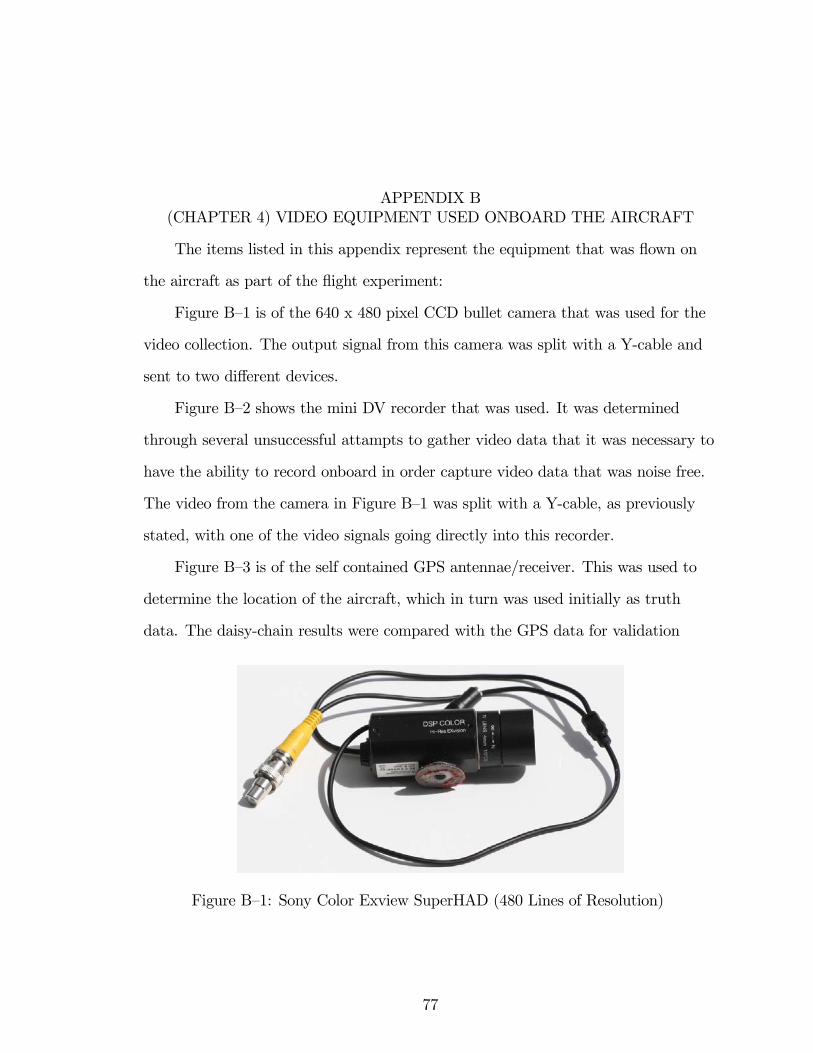
APPENDIX B(CHAPTER 4) VIDEO EQUIPMENT USED ONBOARD THE AIRCRAFT
The items listed in this appendix represent the equipment that was flown on
the aircraft as part of the flight experiment:
Figure B—1 is of the 640 x 480 pixel CCD bullet camera that was used for the
video collection. The output signal from this camera was split with a Y-cable and
sent to two different devices.
Figure B—2 shows the mini DV recorder that was used. It was determined
through several unsuccessful attampts to gather video data that it was necessary to
have the ability to record onboard in order capture video data that was noise free.
The video from the camera in Figure B—1 was split with a Y-cable, as previously
stated, with one of the video signals going directly into this recorder.
Figure B—3 is of the self contained GPS antennae/receiver. This was used to
determine the location of the aircraft, which in turn was used initially as truth
data. The daisy-chain results were compared with the GPS data for validation
Figure B—1: Sony Color Exview SuperHAD (480 Lines of Resolution)
77

78
Figure B—2: Panasonic AG-DV1 Digital Video Recorder
Figure B—3: Garmin GPS 35 OEM GPS Receiver
purposes. The output from this device went to the GPS overlay board shown in
Figure B—4.
Figure B—4 is of the GPS overlay board. The other video signal from the
Y-cable coming from the camera in Figure B—1 went into this board that overlaid
the video with the GPS data from the receiver shown in Figure B—3. From here,
the overlaid video was sent to the transmitter shown in Figure B—5.
Figure B—5 is of the transmitter that was used to send the GPS overlaid video
signal to the ground receiver.

79
Figure B—4: Intuitive Circuits, LLC - OSD-GPS Overlay Board
Figure B—5: 12V, 2.4Ghz, 100mW, Video Transmitter and Antennae

80
Figure B—6: Eagle Tree, Seagull, Wireless Dashboard Flight System - Pro Version:(1) Wireless Telemetry Transmitter, (2) Eagle Tree Systems G-Force Expander, and(3) Eagle Tree Systems GPS Expander
Figure B—6 is of the secondary GPS receiver that was also used for comparison
purposes. This device telemetered the data down on a separate frequency, where it
was recorded on a ground station.

APPENDIX C(CHAPTER 4) GROUND SUPPORT EQUIPMENT
The items listed in this appendix correspond to the ground equipment used in
the flight experiment:
Figure C—1 is of the video receiver that received the GPS overlaid video.
Figure C—2 is of the second video recorder that was used in the testing. In
this case, it was used to record the transmitted GPS overlaid video. The reason
for requiring a second video was that it was necessary to have a clean video
for performing the analysis with (see Figure B—2), yet a method was needed to
correlate each frame of the clean video with a GPS location. Having two recorders
operating at once was the simplest solution. The video that was captured on this
device could not be used for analysis due to the RF noise and the overlay text
that took up much of the image. By doing a frame by frame comparison with the
clean video recorded by the recorder in Figure B—2, it was possible to ascertain the
position of the vehicle to within 1 second (GPS frequency) of every frame of the
clean video.
Figure C—3 is the groundstation interface for the secondary GPS receiver that
was used, shown in Figure B—6.
Figure C—1: RX-2410 2.4 GHz Wireless 4-channel Audio/Video Selectable Receiver
81
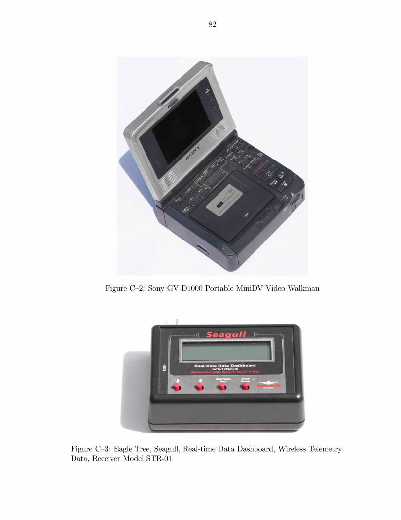
82
Figure C—2: Sony GV-D1000 Portable MiniDV Video Walkman
Figure C—3: Eagle Tree, Seagull, Real-time Data Dashboard, Wireless TelemetryData, Receiver Model STR-01
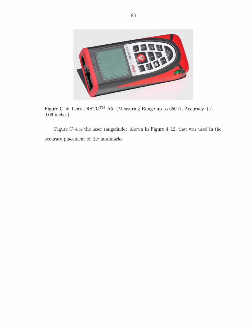
83
Figure C—4: Leica DISTOTM A5 (Measuring Range up to 650 ft, Accuracy +/-0.06 inches)
Figure C—4 is the laser rangefinder, shown in Figure 4—12, that was used in the
accurate placement of the landmarks.

REFERENCES
[1] A. Moutinho and J. R. Azinheira, “Stability and Robustness Analysis of theAURORA Airship Control System Using Dynamic Inversion,”Proceedings ofthe International Conference on Robotics and Automation, Barcelona, Spain,April 2005, pp. 2265—2270.
[2] M. W. Oppenheimer and D. B. Doman, “Control of an Unstable, Nonmini-mum Phase Hypersonic Vehicle Model,” Proceedings of the IEEE AerospaceConference, Big Sky, MT, March 2006, pp. 1-7.
[3] S. Onori, P. Dorato, S. Galeani, and C. Abdallah, “Finite Time Stability De-sign Via Feedback Linearization,” Proceedings of the Conference on Decisionand Control, and the European Control Conference, Seville, Spain, December2005, pp. 4915-4920.
[4] Z. Szabo, P. Gaspar, and J. Bokor, “Tracking Design for Wiener SystemsBased on Dynamic Inversion,” Proceedings of the International Conference onControl Applications, Munich, Germany, October 2006, pp. 1386—1391.
[5] J. Chen, D. Li, X. Jiang, and X. Sun, “Adaptive Feedback LinearizationControl of a Flexible Spacecraft,” Proceedings of the Conference on IntelligentSystems Design and Applications, Jinan, China, October 2006, pp. 225—230.
[6] A. D. Ngo and D. B. Doman, “Dynamic Inversion-Based Adap-tive/Reconfigurable Control of the X-33 on Ascent,” Proceedings of theIEEE Aerospace Conference, Big Sky, MT, March 2006, pp. 2683—2697.
[7] M. D. Tandale and J. Valasek, “Adaptive Dynamic Inversion Control of aLinear Scalar Plant with Constrained Control Inputs,” Proceedings of theAmerican Control Conference, Portland, OR, June 2005, pp. 2064—2069.
[8] N. Hovakimyan, E. Lavretsky, and A. Sasane, “Dynamic Inversion forNonaffine-in-Control Systems Via Time-Scale Separation: Part I,” Pro-ceedings of the American Control Conference, Portland, OR, June 2005, pp.3542—3547.
[9] N. Hovakimyan, E. Lavretsky, and C. Cao, “Dynamic Inversion of MultiinputNonaffine Systems Via Time-Scale Separation,” Proceedings of the AmericanControl Conference, Minneapolis, MN, June 2006, pp. 3594—3599.
84

85
[10] E. Lavretsky and N. Hovakimyan, “Adaptive Dynamic Inversion for Nonaffine-in-Control Systems Via Time-Scale Separation: Part II,” Proceedings of theAmerican Control Conference, Portland, OR, June 2005, pp. 3548—3553.
[11] J. Buffington and A. Sparks, “Comparison of Dynamic Inversion and LPVTailless Flight Control Law Designs,” Proceedings of the American ControlConference, vol. 2, Philadelphia, PA, June 1998, pp. 1145—1149.
[12] X.-. J. Liu, F. Lara-Rosano, and C. W. Chan, “Model-Reference AdaptiveControl Based on Neurofuzzy Networks,” IEEE Trans. Syst., Man, Cybern. C,vol. 34, no. 3, pp. 302—309, August 2004.
[13] A. Calise and R. Rysdyk, “Nonlinear Adaptive Flight Control Using NeuralNetworks,” IEEE Control System Magazine, vol. 18, no. 6, pp. 14—25, Decem-ber 1998.
[14] J. Leitner, A. Calise, and J. V. R. Prasad, “Analysis of Adaptive NeuralNetworks for Helicopter Flight Controls,” AIAA Journal of Guidance, Control,and Dynamics, vol. 20, no. 5, pp. 972—979, September 1997.
[15] Y. Shin, “Neural Network Based Adaptive Control for Nonlinear DynamicRegimes,” Ph.D. dissertation, Georgia Technical Institute, November 2005.
[16] E. Lavretsky and N. Hovakimyan, “Adaptive Compensation of Control Depen-dent Modeling Uncertainties Using Time-Scale Separation,” Proceedings of theConference on Decision and Control, and the European Control Conference,Seville, Spain, December 2005, pp. 2230—2235.
[17] B. Xian, D. M. Dawson, M. S. de Queiroz, and J. Chen, “A ContinuousAsymptotic Tracking Control Strategy for Uncertain Nonlinear Systems,”IEEE Transactions on Automatic Control, vol. 49, no. 7, pp. 1206—1211, July2004.
[18] P. M. Patre, W. MacKunis, C. Makkar, and W. E. Dixon, “AsymptoticTracking for Systems with Structured and Unstructured Uncertainties,”Proceedings of the Conference on Decision and Control, San Diego, CA,December 2006, pp. 441—446.
[19] Z. Cai, M. S. de Queiroz, and D. M. Dawson, “Robust Adaptive AsymptoticTracking of Nonlinear Systems with Additive Disturbance,” IEEE Transac-tions on Automatic Control, vol. 51, no. 3, pp. 524—529, March 2006.
[20] B. Xian, M. S. de Queiroz, and D. M. Dawson, A Continuous Control Mecha-nism for Uncertain Nonlinear Systems in Optimal Control, Stabilization, andNonsmooth Analysis, Heidelberg, Germany: Springer-Verlag, 2004.
[21] X. Zhang, A. Behal, D. M. Dawson, and B. Xian, “Output Feedback Controlfor a Class of Uncertain MIMO Nonlinear Systems with Nonsymmetric Input

86
Gain Matrix,” Proceedings of the Conference on Decision and Control, and theEuropean Control Conference, Seville, Spain, December 2005, pp. 7762—7767.
[22] M. L. McIntyre, W. E. Dixon, D. M. Dawson, and I. D. Walker, “FaultIdentification for Robot Manipulators,” IEEE Transactions on Robotics andAutomation, vol. 21, no. 5, pp. 1028—1034, October 2005.
[23] S. Gupta, D. Aiken, G. Hu, and W. E. Dixon, “Lyapunov-Based Rangeand Motion Identification for a Nonaffine Perspective Dynamic System,”Proceedings of the American Control Conference, Minneapolis, MN, June 2006,pp. 4471—4476.
[24] W. E. Dixon, Y. Fang, D. M. Dawson, and T. J. Flynn, “Range Identificationfor Perspective Vision Systems,” IEEE Transactions on Automatic Control,vol. 48, no. 12, pp. 2232—2238, December 2003.
[25] A. Behal, D. M. Dawson, W. E. Dixon, and Y. Fang, “Tracking and Reg-ulation Control of an Underactuated Surface Vessel with NonintegrableDynamics,” Proceedings of the Conference on Decision and Control, vol. 3,Sydney, Australia, December 2000, pp. 2150—2155.
[26] Center, J. A. V. N. T. S., “Vulnerability Assessment of the Transport In-frastructure Relying on the Global Positioning System,” Report, Office of theAssistant Secretary for Transportation Policy, U.S. Department of Transporta-tion, August 2001.
[27] G. Hu, S. Mehta, N. R. Gans, W. E. Dixon, "Daisy Chaining Based VisualServo Control Part I: Adaptive Quaternion-Based Tracking Control ," Proceed-ings of the IEEE Multi-conference on Systems and Control, Singapore, October2007, pp. 1474—1479.
[28] G. Hu, N. R. Gans, S. Mehta, W. E. Dixon, "Daisy Chaining Based VisualServo Control Part II: Extensions, Applications and Open Problems," Pro-ceedings of the IEEE Multi-conference on Systems and Control, Singapore,October 2007, pp. 729—734.
[29] Roberts, J. M., Corke, P. I., and Buskey, G., “Low-Cost Flight ControlSystem for a Small Autonomous Helicopter,” Proceedings of the AustralasianConference on Robotics and Automation, Auckland, New Zealand, November,2002.
[30] Zhang, H. and Ostrowski, J., “Visual Servoing with Dynamics: Control ofan Unmanned Blimp,” Proceedings of the IEEE International Conference onRobotics and Automation, vol. 1, May 1999, pp. 618—623.
[31] Sharp, C. S., Shakernia, O., and Sastry, S. S., “A Vision System for Land-ing an Unmanned Aerial Vehicle,” Proceedings of the IEEE International

87
Conference on Robotics and Automation (ICRA), Seoul, Korea, 2001, pp.1720—1727.
[32] Bernatz, A., and Thielecke, F., “Navigation of a Low Flying VTOL AircraftWith the Help of a Downwards Pointing Camera,” Proceedings of the AIAAGuidance, Navigation, and Control Conference, Providence, RI, August 2004.
[33] Yuan, Z., Gong, Z., Wu, J., Chen, J., and Rao, J., “A Real-Time Vision-basedGuided Method forAutonomous Landing of a Rotor-craft Unmanned AerialVehicle,” Proceedings of the IEEE International Conference on Mechatronics &Automation, Niagara Falls, Canada, July 2005, pp 2212—2215.
[34] Wu, A. D., Johnson, E. N., and Proctor, A. A., “Vision-Aided InertialNavigation for Flight Control,” Journal of Aerospace Computing, Information,and Communication, vol. 2, September 2005, pp. 348—360.
[35] Schulz, H.-W., Buschmann, M., Krüger, L., Winkler, S., and Vörsmann, P.,“Vision-Based Autonomous Landing for Small UAVs — First ExperimentalResults,” Infotech@Aerospace, Arlington, Virginia, September, 2005.
[36] Jones, C. G., Heyder-Bruckner, J. F., Richardson, T. S., and Jones, D. C.,“Vision-based Control for Unmanned Rotorcraft,” Proceedings of the AIAAGuidance, Navigation, and Control Conference, AIAA-2006-6684, Keystone,CO, August 2006.
[37] Saripalli, S., Montogomery, J. F., and Sukhatme, G. S., “Visually GuidedLanding of an Unmanned Aerial Vehicle,” IEEE Transactions on Robotics andAutomation, vol. 19, No. 3, June 2003, pp. 371—380.
[38] Chatterji, G. B., Menon, P. K., and Sridhar, B., “Vision-Based Position andAttitude Determination for Aircraft Night Landing,” Journal of Guidance,Control, and Dynamics, 1998 vol. 21, No. 1, pp. 84—92.
[39] Proctor, A. A., and Johnson, E. N., “Vision-only Approach and Landing,”Proceedings of the AIAA Guidance, Navigation, and Control Conference,AIAA-2005-5871, San Francisco, CA, August 2005.
[40] Liu, T., and Fleming, G., “Videogrammetric Determination of Aircraft Posi-tion and Attitude for Vision-Based Autonomous Landing,” AIAA AerospaceSciences Meeting and Exhibit, AIAA-2006-1437, Reno, NV, January 2006.
[41] Shakernia, O., Y. Ma, Koo, T. J., and Sastry, S., “Landing an UnmannedAir Vehicle: Vision Based Motion Estimation and Nonlinear Control,” AsianJournal of Control, vol 1, pp. 128—145.
[42] Jianchao, Y., “A New Scheme of Vision Based Navigation for Flying Vehicles- Concept Study and Experiment Evaluation,” Proceedings of the IEEE
88
International Conference on Control, Automation, Robotics And Vision(ICARV), Singapore, December 2002, pp. 643—648.
[43] Kim, J., “Autonomous Navigation for Airborne Applications,” Ph.D. Disserta-tion, Department of Aerospace, Mechanical and Mechatronic Engineering, TheUniversity of Sydney, Sydney, Australia, May 2004.
[44] Webb, T. P., Prazenica, R. J., Kurdila, A. J., and Lind, R., “Vision-BasedState Estimation for Uninhabited Aerial Vehicles,” Proceedings of the AIAAGuidance, Navigation, and Control Conference, AIAA-2005-5869, San Fran-cisco, CA, August 2005.
[45] Prazenica, R. J., Watkins, A., Kurdila, A. J., Ke, Q. F., and Kanade, T.,“Vision-Based Kalman Filtering for Aircraft State Estimation and Structurefrom Motion,” Proceedings of the AIAA Guidance, Navigation, and ControlConference, AIAA-2005-6003, San Francisco, CA, August 2005.
[46] Caballero, F., Merino, L., Ferruz, J., and Ollero, A., “Improving Vision-BasedPlanar Motion Estimation for Unmanned Aerial Vehicles Through OnlineMosaicing,” Proceedings of the IEEE International Conference on Robotics andAutomation (ICRA), May 2006, pp. 2860—2865.
[47] Koch, A., Wittich, H., and Thielecke, F., “A Vision-Based Navigation Algo-rithm for a VTOL-UAV,” Proceedings of the AIAA Guidance, Navigation, andControl Conference, AIAA-2006-6546, Keystone, CO, August 2006.
[48] Barber, D. B., Griffiths, S. R., McLain, T. W., and Beard, R. W., “Au-tonomous Landing of Miniature Aerial Vehicles,” Journal of AerospaceComputing, Information, and Communication, vol. 4, May 2007, p. 770.
[49] Trisiripisal, P., Parks, M. R., Abbot, A. L., Liu, T., and Fleming, G. A.,“Stereo Analysis for Vision-based Guidance and Control of Aircraft Landing,”Proceedings of the AIAA Aerospace Sciences Meeting and Exhibit, AIAA-2006-1438, Reno, Nevada, January 2006.
[50] A. Chiuso, P. Favaro, H. Jin, and S. Soatto, “Structure from Motion CausallyIntegrated Over Time,” IEEE Transactions on Pattern Analysis and MachineIntelligence, vol. 24, pp. 523—535, 2002.
[51] H. Kano, B. K. Ghosh, and H. Kanai, “Single Camera Based Motion andShape Estimation Using Extended Kalman Filtering,” Mathematical andComputer Modelling, vol. 34, pp. 511—525, 2001.
[52] L. Matthies, T. Kanade, and R. Szeliski, “Kalman Filter-Based Algorithm forEstimating Depth from Image Sequence,” International Journal of ComputerVision, vol. 3, pp. 209—236, 1989.

89
[53] S. Soatto, R. Frezza, and P. Perona, “Motion Estimation Via DynamicVision,” IEEE Transactions on Automatic Control, vol. 41, pp. 393—413, 1996.
[54] X. Chen and H. Kano, “State Observer for a Class of Nonlinear Systems andits Application to Machine Vision,” IEEE Transactions on Automatic Control,vol. 49, no. 11, pp. 2085—2091, 2004.
[55] X. Chen and H. Kano, “A New State Observer for Perspective Systems,” IEEETransactions on Automatic Control, vol. 47, no. 4, pp. 658—663, 2002.
[56] W. E. Dixon, Y. Fang, D. M. Dawson, and T. J. Flynn, “Range Identificationfor Perspective Vision Systems,” IEEE Transactions on Automatic Control,vol. 48, no. 12, pp. 2232—2238, 2003.
[57] M. Jankovic and B. K. Ghosh, “Visually Guided Ranging from Observations ofPoints, Lines and Curves Via an Identifier Based Nonlinear Observer,” Systemsand Control Letters, vol. 25, pp. 63—73, 1995.
[58] D. Karagiannis and A. Astolfi, “A New Solution to the Problem of RangeIdentification in Perspective Vision Systems,” IEEE Transactions on Auto-matic Control, vol. 50, pp. 2074—2077, 2005.
[59] L. Ma, Y. Chen, and K. L. Moore, “Range Identification for PerspectiveDynamic System with Single Homogeneous Observation,” Proceedings of theIEEE. International Conference on Robotics Automation, 2004, pp. 5207—5212.
[60] ––, “Range Identification for Perspective Dynamic System Using LinearApproximation,” Proceedings of the IEEE International Conference onRobotics Automation, 2004, pp. 1658—1663.
[61] Ashley, H., and Landahl, M., Aerodynamics of Wings and Bodies, DoverPublications, Inc., 1985.
[62] Z. Cai, M. S. de Queiroz, D. M. Dawson, and B. Xian, “Adaptive AsymptoticTracking of Parametric Strict-Feedback Systems in the Presence of AdditiveDisturbances,” 43rd IEEE Conference on Decision and Control, December14-17, 2004.
[63] L. Duan, W. Lu, F. Mora-Camino, and T. Miquel, “Flight-Path TrackingControl of a Transportation Aircraft: Comparison of Two Nonlinear De-sign Approaches,” Proceedings of the Digital Avionics Systems Conference,Portland, OR, October 2006, pp. 1—9.
[64] I. Szaszi, B. Kulcsar, G. J. Balas, and J. Bokor, “Design of FDI Filter for anAircraft Control System,” Proceedings of the American Control Conference,Anchorage, AK, May 2002, pp. 4232—4237.
[65] Department of Transportation, “Airworthiness Standards: Transport CategoryAirplanes,” Federal Aviation Regulations - Part 25, Washington, DC, 1996.
90
[66] F. L. Lewis, C. T. Abdallah, and D. M. Dawson, Control of Robot Manipula-tors, New York, NY: MacMillan, 1993.
[67] B. S. Davis, T. Denison, and J. Kaung, “A Monolithic High-g SOI-MEMSAccelerometer for Measuring Projectile Launch and Flight Accelerations,”Proceedings of the Conference on Sensors, Vienna, Austria, October 2004, pp.296—299.
[68] V. Janardhan, D. Schmitz, and S. N. Balakrishnan, “Development andImplementation of New Nonlinear Control Concepts for a UA,” Proceedings ofthe Digital Avionics Systems Conference, Salt Lake City, UT, October 2004,pp. 12.E.5—121—10.
[69] T. Wagner and J. Valasek, “Digital Autoland Control Laws Using QuantitativeFeedback Theory and Direct Digital Design,” AIAA Journal of Guidance,Control, and Dynamics, vol. 30, no. 5, pp. 1399—1413, September 2007.
[70] M. Bodson, “Multivariable Adaptive Algorithms for Reconfigurable FlightControl,” Proceedings of the Conference on Decision and Control, Lake BuenaVista, FL, December 1994, pp. 12.E.5—121—10.
[71] B. J. Bacon, A. J. Ostroff, and S. M. Joshi, “Reconfigurable NDI ControllerUsing Inertial Sensor Failure Detection & Isolation,” IEEE Transactions onAerospace Electronic Systems, vol. 37, no. 4, pp. 1373—1383, Oct. 2001.
[72] G. Tao, Adaptive Control Design and Analysis, S. Haykin, Ed., New York:Wiley-Interscience, 2003.
[73] D. Dawson, M. Bridges, and Z. Qu, Nonlinear Control of Robotic Systems forEnvironmental Waste and Restoration, Englewood Cliffs, NJ: Prentice HallPTR, 1995.
[74] H. K. Khalil, Nonlinear Systems, Third Edition, Upper Saddle River, NJ:Prentice Hall, 2002.
[75] P. M. Patre, W. MacKunis, C. Makkar, and W. E. Dixon, “AsymptoticTracking for Systems with Structured and Unstructured Uncertainties,”IEEE Transactions on Control Systems Technology, vol. 16, March 2008, pp.373—379.
[76] Kaiser, M. K., Gans, N. R., and Dixon, W. E., “Position and Orientationof an Aerial Vehicle through Chained, Vision-Based Pose Reconstruction,”Proceedings of the AIAA Guidance, Navigation, and Control Conference,Keystone, CO, 2006.
[77] Kaiser, M. K., Gans, N. R., and Dixon, W. E., “Localization and Controlof an Aerial Vehicle through Chained,Vision-Based Pose Reconstruction,”Proceedings of the American Control Conference, New York, NY, 2007.

91
[78] Longuet-Higgins, H., “A Computer Algorithm for Reconstructing a Scene fromTwo Projections,” Nature, Sept. 1981, pp. 133—135.
[79] Hartley, R., Computer Vision Proc. of 1992 European Conference on ComputerVision, Lecture Notes in Computer Sciences, New York: Springer-Verlag, 1992.
[80] Nister, D., “An Efficient Solution to the Five-Point Relative Pose Problem,”IEEE Transactions on Pattern Analysis and Machine Intelligence, vol. 26,June 2004, pp. 756—770.
[81] Ma, Y., Soatto, S. Kosecká, J., and Sastry, S., An Invitation to 3-D Vision,New York: Springer, 2004.
[82] Faugeras, O., and Lustman, F., “Motion and Structure from Motion in aPiecewise Planar Environment,” International Journal of Pattern Recognitionand Artificial Intelligence, vol. 2, No. 3, 1988, pp. 485—508.
[83] Zhang, Z., and Hanson, A., “3D Reconstruction Based on HomographyMapping,” Proceedings of the ARPA Image Understanding Workshop, PalmSprings, CA, 1996.
[84] S. Soatto and P. Perona, “Reducing "Structure from Motion": A GeneralFramework for Dynamic Vision Part 1: Modeling,” IEEE Transactions onPattern Analysis and Machine Intelligence, vol. 20, no. 9, pp. 933—942, 1998.
[85] ––, “Reducing "Structure from Motion": A General Framework for Dy-namic Vision Part 2: Implementation and Experimental Assessment,” IEEETransactions on Pattern Analysis and Machine Intelligence, vol. 20, no. 9, pp.943—960, 1998.
[86] R. Y. Tsai and T. S. Huang, “Estimating Three-Dimensional Motion Para-meters of a Rigid Planar Patch,” IEEE Transactions on Acoustics, Speech, &Signal Processing, vol. 29, no. 6, pp. 1147—1152, 1981.
[87] D. Aiken, S. Gupta, G. Hu, and W. E. Dixon, “Lyapunov-Based RangeIdentification for a Paracatadioptric System,” Proceedings of the IEEEConference on Decision and Control, 2006, pp. 3879—3884.
[88] L. Ma, Y. Chen, and K. L. Moore, “Range Identification for PerspectiveDynamic Systems with 3D Imaging Surfaces,” Proceedings of the AmericanControl Conference, 2005, pp. 3671—3675.
[89] S. Gupta, D. Aiken, G. Hu, and W. E. Dixon, “Lyapunov-Based Rangeand Motion Identification for a Nonaffine Perspective Dynamic System,”Proceedings of the American Control Conference, 2006, pp. 4471—4476.
[90] J. J. Slotine and W. Li, Applied Nonlinear Control. Englewood Cliffs, NJ:Prentice Hall, 1991.
BIOGRAPHICAL SKETCH
Kent Kaiser received a B.S. degree in aerospace engineering from Auburn
University in 1990, an M.S. degree in mechanical engineering from the University
of Houston in 1995, and completed coursework towards an additional M.S. degree
in aerodynamics and propulsion engineering from Cal Poly Pomona. He has
nearly 20 years work experience within the aerospace industry, which includes his
current employment with Air Force Research Labs (AFRL), as well as previous
employment with Lockheed Martin Corporation in Houston, TX, Palmdale, CA,
and Marietta, GA. Some of his research interests include system identification,
aerodynamic performance based design, flight dynamics and control, neural
net-based adaptive control, proper orthogonal decomposition (POD) for fluidic
modeling and flow control, robust control, micro-UAVs, linear matrix inequality
(LMI) control, nonlinear dynamic inversion methods for aircraft control, vision-
based estimation, guidance, and control, and cooperative control.
92