Embed Size (px)
Citation preview
J Comput Neurosci (2009) 26:219–249DOI 10.1007/s10827-008-0108-4
Virtual Retina: A biological retina modeland simulator, with contrast gain control
Adrien Wohrer · Pierre Kornprobst
Received: 16 May 2007 / Revised: 14 May 2008 / Accepted: 16 June 2008 / Published online: 1 August 2008© Springer Science + Business Media, LLC 2008
Abstract We propose a new retina simulation software,called Virtual Retina, which transforms a video intospike trains. Our goal is twofold: Allow large scale sim-ulations (up to 100,000 neurons) in reasonable process-ing times and keep a strong biological plausibility,taking into account implementation constraints. Theunderlying model includes a linear model of filtering inthe Outer Plexiform Layer, a shunting feedback at thelevel of bipolar cells accounting for rapid contrast gaincontrol, and a spike generation process modeling gan-glion cells. We prove the pertinence of our software byreproducing several experimental measurements fromsingle ganglion cells such as cat X and Y cells. Thissoftware will be an evolutionary tool for neuroscientiststhat need realistic large-scale input spike trains in sub-sequent treatments, and for educational purposes.
Keywords Large-scale retina simulator ·Contrast gain control · Spikes · Conductances
1 Introduction
The simulator Virtual Retina1 is fully documented anddownloadable.2 As an alternative solution to down-
Action Editor: Alexander Borst
A. Wohrer · P. Kornprobst (B)Odyssée project team (INRIA/ENPC/ENS), INRIA,Sophia-Antipolis, 2004 Route des Lucioles,06902 Sophia Antipolis, Francee-mail: [email protected]
A. Wohrere-mail: [email protected]
loading, the software homepage also includes a webservice3 which allows clients to use the simulator on-line, through a user-friendly interface requiring no in-stallation.
The simulator is mostly based on state-of-the-artknowledge about retinal processing, with formulationsadapted to large-scale simulation. Modular XML de-finition files provide a simple handling of the simula-tor’s different parameters. In this article, we detail theunderlying model and the interesting features of thesimulator.
Retina (and LGN) models are very numerous, rank-ing from detailed models of a specific physiologi-cal phenomenon, to large-scale models of the wholeretina. However, interestingly, the category of large-scale models appears under-represented in retinal liter-ature. The reason is simple: On one side, experimentalresearchers on the retina are not very interested inlarge-scale models that require mostly a compilationof already well-established results. On the other side,researchers that seek a retina/LGN input for furthermodeling (typically, of V1) often overlook the complex-ity of processing in the retina, and use very simplifiedretina models.
1Under INRIA CeCILL C open-source license, IDDN numberIDDN.FR.001.210034.000.S.P.2007.000.31235.2Homepage: http://www-sop.inria.fr/odyssee/software/virtualretina/.3Server address: http://facets.inria.fr/retina/webservice.html, alsoaccessible directly from the software homepage.

220 J Comput Neurosci (2009) 26:219–249
Our primary goal with Virtual Retina is to providea better retinal input to modelers of the visual cortex.Retinal processing displays a number of features whichare likely fundamental for further cortical interpreta-tion, such as band-pass filtering, gain controls, spikingsynchrony, etc. (Wohrer 2008b) It is these functionalimplications of retinal processing that we wanted toretain in the simulator. This focus on functionalitynaturally makes Virtual Retina a good candidate for asecond type of application: to study the nature of theretinal code itself.
By opposition, reproducing biological complexity isnot our primary goal. However, because the retina isan efficient machinery, a functional model to reproduceretinal specificities must de facto have an architecturequite close to that of a real retina, to allow the samesort of filtering operations.
Amongst models of retinal processing as a whole,some focus on a detailed reproduction of retinal con-nectivity in successive layers, each layer being mod-eled with a full set of cellular and synaptic parameters(Hennig et al. 2002; Bálya et el. 2002). Other modelstake a more functional approach, built on a seriesof specific filtering stages, to produce a functionallyefficient retinal output. In this group, another distinc-tion can be made between models that aim at strongbiological precision (van Hateren et al. 2002; Gazereset al. 1998; Bonin et al. 2005), and models more ori-ented towards signal processing and computer vision(Hérault and Durette 2007; Delorme et al. 1999), witha consequent reduction of model parameters. Manyfunctional models are strongly inspired by the linear–nonlinear (LN) architecture, based on three successivestages: Linear filtering on the visual stimulus, staticnonlinearity and then spike generation (Chichilnisky2001). Because of their generality and wide use, LNmodels have even been termed the retinal standardmodel by Carandini et al. (2005).
For Virtual Retina, we propose a model somewherein-between all models cited above. It is definitely afunctional model, with consequent simplifications re-garding the complexity of retinal physiology. Still, itaims at a relative biological precision: This is verifiedby reproducing different experimental recordings onreal retinal ganglion cells, including experiments notaccounted for by linear models.
LN models are also a strong inspiration to our model:The first stage consists of a spatio-temporal linear filter,and we make use of static nonlinearities. However, asopposed to LN models, we also incorporate a nonlin-ear mechanism of contrast gain control, inspired fromretinal physiology and other existing models. Further-
more, whereas LN models are generally used to ex-perimentally fit the responses of a few ganglion cells(Chichilnisky 2001; Keat et al. 2001; Baccus and Meister2002), we propose here a functional model suitable forlarge-scale simulation.
More generally, the model keeps an architecturestrongly related to retinal physiology, in a desire toreproduce specific effects which are functionally impor-tant, and often discarded by large-scale models:
• Non-separability of the center-surround filtering.It is well-known that most ganglion cells have acenter-surround receptive field organization whichmakes them more sensitive to image edges. In realretinas, the surround signal is transmitted with asupplementary delay of a few milliseconds. This de-lay is included in our software, since it yields conse-quent effects for the perception of uniform screens,or appearing images. A qualitative, large-scale illus-tration of this fact is provided in the article.
• Contrast gain control. This specific nonlinear de-pendence of retinal filtering on the mean levelof contrast is modeled in an original framework,inspired by previous models, that can account si-multaneously for gain controls due to the temporaland spatial structure of the stimulus. This contrastgain control model is carefully discussed, justifiedmathematically, and its perceptual consequencesare suggested through a qualitative simulation.
• Adaptable band-pass temporal filtering. In theretina, some ganglion cells have a long-lasting re-sponse after apparition of a static visual stimulus(tonic cells), while others only respond by a strongand short activation wave right after stimulus onset,and return to being silent afterward (phasic cells).Virtual Retina accounts for both types of cells in thesimplest way possible, by modifying the strength ofa partially high-pass filter.
• Spike generation mechanism. A possible spike gen-eration process is proposed at the output of thesoftware, with a model derived from experimentalfitting of ganglion cell outputs (Keat et al. 2001),that yields more realistic spike trains than a Poissonprocess.
None of the previously cited models of retinal process-ing displays simultaneously all these elements. Furthercapabilities of the software include reproduction ofY-type cells’ spatial nonlinearity (Enroth-Cugell andRobson 1966; Enroth-Cugell and Freeman 1987) anda possible log-polar scheme modeling the large-scaleorganization of primate retinas.
J Comput Neurosci (2009) 26:219–249 221
The article is organized as follows. In Section 2,we detail the three stages of the retina model imple-mented by the simulator. The first stage (2.2) is a linearfilter that reproduces the center-surround architecturearising from the interaction between light receptors andhorizontal cells. The second stage (2.3) is a contrastgain control mechanism at the level of bipolar cells,driven by feedback conductances. The third stage (2.4)provides additional temporal shaping of the signal, andthen a spike generation process. Based on this model,we present in Section 3 the software simulator, Vir-tual Retina, and the results that we obtain with vari-ous sequences. First, we prove the pertinence of ourmodel by comparing its spiking output with recordingsof ganglion cells in different experiments (3.2). Then,we show large-scale simulations and more qualitativeresults (3.3). Finally, in Section 4, we discuss the natureof the software and its underlying model (4.1), andmore specifically the included contrast gain controlmechanism (4.2).
2 Methods
2.1 General structure of the model
2.1.1 A layered model in three stages
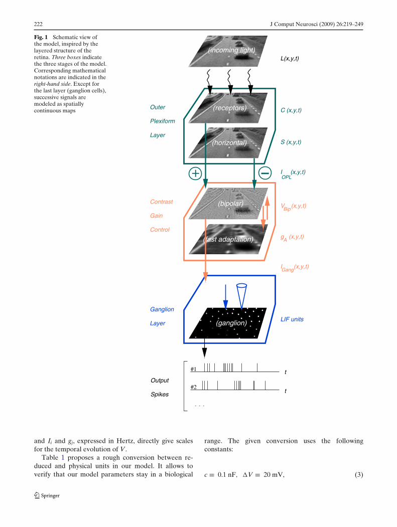
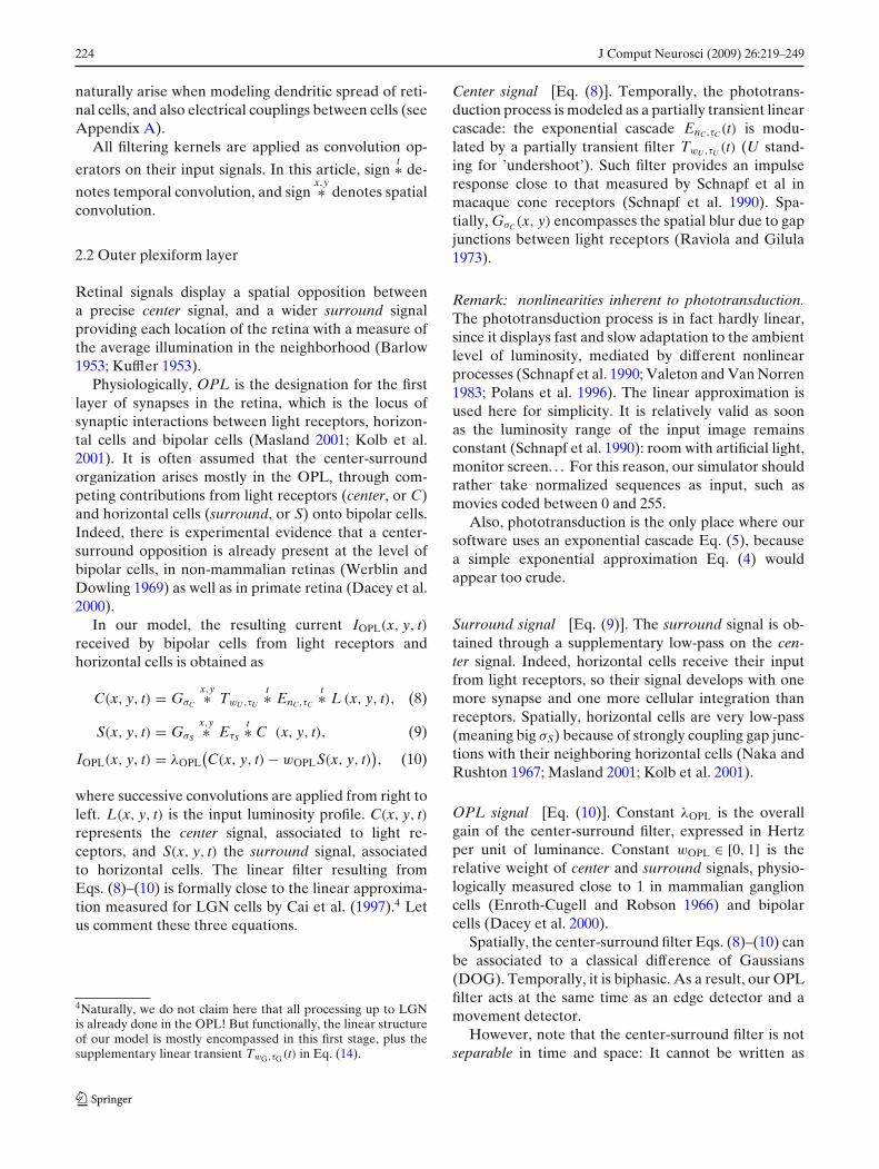
Figure 1 presents the global architecture of our model.The layered architecture of a retina suggests a modelmade of successive continuous spatio-temporal mapsthat progressively transmit and transform the incomingsignal. The incoming light on the retina is the luminosityprofile L(x, y, t) defined for every spatial point (x, y) ofthe retina at each time t. It can have any units in ourmodel; for our simulations we used digitalized intensi-ties between 0 and 255. The subsequent layers of cellsare modeled as spatial continuums (no discrete cells,except the output ganglion cells), driven by specificdifferential equations.
The first stage of our model deals with signal process-ing done in the Outer Plexiform Layer (OPL). It in-volves the two first layers of cells in the retina: lightreceptors and horizontal cells. This stage is modeled asa simple spatio-temporal linear filter based on experi-mental recordings (Enroth-Cugell et al. 1983; Cai et al.1997) and previous models (Mahowald and Mead 1991;Herault 1996). We detail this OPL filter in Section 2.2.When applied to the input sequence L(x, y, t), the OPLfilter defines a band-pass excitatory current IOPL(x, y, t)which is fed to bipolar cells.
The second stage of the model is an instantaneous,nonlinear contrast gain control through a variable feed-back shunt conductance gA(x, y, t), applied on bipolarcells in our model. This interaction is represented bythe two small arrows between bipolar cells and the ’fastadaptation’ signal in Fig. 1.
The third stage models signal processing in the InnerPlexiform Layer (IPL) and ganglion cells. First, addi-tional spatio-temporal shaping of the signal is provided,modeling some synaptic interactions in the IPL. It pro-duces the excitatory current IGang, which is fed to ourmodel ganglion cells. Second, ganglion cells themselvesare modeled as a discrete set of noisy integrate-and-fire (nLIF) cells paving the visual field, and generat-ing spike trains from input current IGang. The cellsthat we model (see Sections 3.2.1 and 4.1.2) can beeither X-type (the blue arrow, representing a one-to-one connection from bipolar cells) or Y-type (the bluecone, representing a synaptic pooling of the excitatorycurrent).
2.1.2 Dimensional reduction
Our model equivalents to bipolar cells (Section 2.3)and ganglion cells (Section 2.4) are based on the same,generic membrane equation for a point neuron:
cdVdt
=∑
i
Ii +∑
j
g j(E j − V). (1)
V is the cell’s membrane potential in Volts, c is themembrane capacity in Farads. Synaptic inputs (andother intrinsic membrane currents) can either be mod-eled as currents Ii in Amperes, or more precisely assynaptic conductances g j in Siemens associated to re-versal potentials E j in Volts.
Since our model does not focus on physiologicalprecision, but on the functional output of the retina ona large scale, we are solely concerned with the tempo-ral evolution induced by Eq. (1). Hence the followingreduction of dimensionality:
V → (V − VR)/�V, I → I/(c�V), g → g/c, (2)
where c is the membrane capacity of the neuron, VR itsresting potential, and �V a ‘typical’ range of variationfor the neurons’ potential. Through this reduction, con-stant c disappears from Eq. (1), V and the E j becomedimensionless with typical values the order of unity,
222 J Comput Neurosci (2009) 26:219–249
Fig. 1 Schematic view ofthe model, inspired by thelayered structure of theretina. Three boxes indicatethe three stages of the model.Corresponding mathematicalnotations are indicated in theright-hand side. Except forthe last layer (ganglion cells),successive signals aremodeled as spatiallycontinuous maps
#1
#2
(incoming light)
(receptors)
(horizontal)
(bipolar)
(ganglion)
_+
(fast adaptation)
t
tSpikes
Output
Layer
Outer
Plexiform
V (x,y,t)Bip
I (x,y,t)Gang
Layer
Ganglion
Control
Contrast
Gain
L(x,y,t)
OPLI (x,y,t)
LIF units
C (x,y,t)
S (x,y,t)
Ag (x,y,t)
and Ii and gj, expressed in Hertz, directly give scalesfor the temporal evolution of V.
Table 1 proposes a rough conversion between re-duced and physical units in our model. It allows toverify that our model parameters stay in a biological
range. The given conversion uses the followingconstants:
c ≡ 0.1 nF, �V ≡ 20 mV, (3)
J Comput Neurosci (2009) 26:219–249 223
Table 1 Rough conversion between physical and reduced unitsin the model, based on Eqs. (2)–(3)
Magnitude V (potential) I (current) G (conductance)
Reduced units 1 (no unit) 1 Hz 1 HzPhysical units 20 mV 2 pA 0.1 nS
in link with physiological measurements in mam-malian bipolar (Euler and Masland 2000) and ganglion(O’Brien et al. 2002) cells.
2.1.3 Notations for linear filters
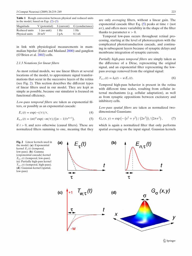
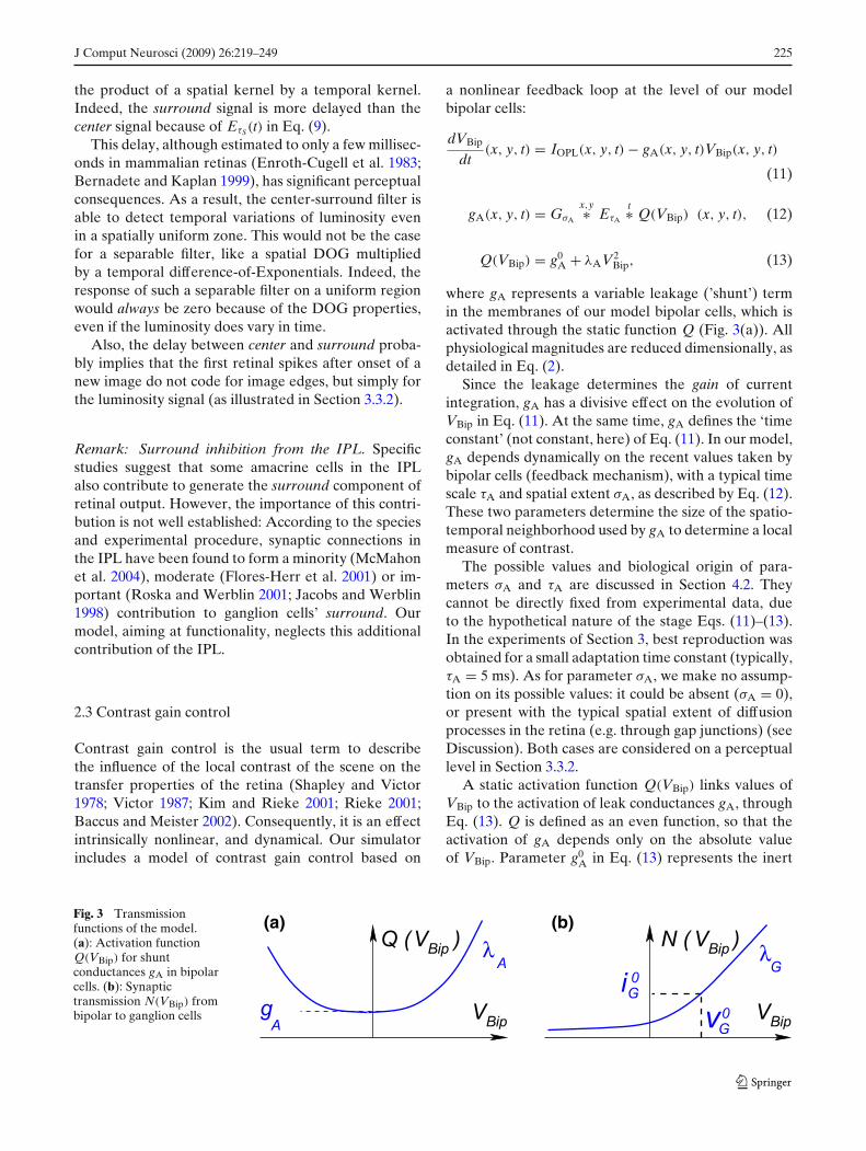
As most retinal models, we use linear filters at severallocations of the model, to approximate signal transfor-mations that occur in the successive layers of the retina(see Fig. 2). This section describes the different typesof linear filters used in our model. They are kept assimple as possible, because our simulator is focused onfunctional efficiency.
Low-pass temporal filters are taken as exponential fil-ters, or possibly as an exponential cascade:
Eτ (t) = exp(−t/τ)/τ, (4)
En,τ (t) = (nt)n exp(−nt/τ)/((n − 1)!τ n+1
), (5)
if t > 0, and zero otherwise (causal filters). These arenormalized filters summing to one, meaning that they
are only averaging filters, without a linear gain. Theexponential cascade filter Eq. (5) peaks at time τ (notnτ ), and offers more variability in the shape of the filterthanks to parameter n > 0.
Temporal low-pass occurs throughout retinal pro-cessing, starting at the level of photoreceptors with thecomplicated phototransduction cascade, and continu-ing in subsequent layers because of synaptic delays andmembrane integration of synaptic currents.
Partially high-pass temporal filters are simply taken asthe difference of a Dirac, representing the originalsignal, and an exponential filter representing the low-pass average removed from the original signal:
Tw,τ (t) = δ0(t) − wEτ (t). (6)
Temporal high-pass behavior is present in the retinawith different time scales, resulting from cellular in-ternal mechanisms (e.g. cellular adaptation), as wellas from synaptic oppositions between excitatory andinhibitory cells.
Low-pass spatial filters are taken as normalized two-dimensional Gaussians:
Gσ (x, y) = exp(− (
x2 + y2)/(2σ 2
))/(2πσ 2
), (7)
which is again a normalized filter that only performsspatial averaging on the input signal. Gaussian kernels
Fig. 2 Linear kernels used inthe model. (a): Exponentialkernel Eτ (t) (temporal,low-pass). (b): Gamma(exponential cascade) kernelEn,τ (t) (temporal, low-pass).(c): Partially high-pass kernelTw,τ (t) (temporal, high-pass).(d): Gaussian kernel (spatial,low-pass)
224 J Comput Neurosci (2009) 26:219–249
naturally arise when modeling dendritic spread of reti-nal cells, and also electrical couplings between cells (seeAppendix A).
All filtering kernels are applied as convolution op-
erators on their input signals. In this article, signt∗ de-
notes temporal convolution, and signx,y∗ denotes spatial
convolution.
2.2 Outer plexiform layer
Retinal signals display a spatial opposition betweena precise center signal, and a wider surround signalproviding each location of the retina with a measure ofthe average illumination in the neighborhood (Barlow1953; Kuffler 1953).
Physiologically, OPL is the designation for the firstlayer of synapses in the retina, which is the locus ofsynaptic interactions between light receptors, horizon-tal cells and bipolar cells (Masland 2001; Kolb et al.2001). It is often assumed that the center-surroundorganization arises mostly in the OPL, through com-peting contributions from light receptors (center, or C)and horizontal cells (surround, or S) onto bipolar cells.Indeed, there is experimental evidence that a center-surround opposition is already present at the level ofbipolar cells, in non-mammalian retinas (Werblin andDowling 1969) as well as in primate retina (Dacey et al.2000).
In our model, the resulting current IOPL(x, y, t)received by bipolar cells from light receptors andhorizontal cells is obtained as
C(x, y, t) = GσC
x,y∗ TwU ,τU
t∗ EnC,τC
t∗ L (x, y, t), (8)
S(x, y, t) = GσS
x,y∗ EτS
t∗ C (x, y, t), (9)
IOPL(x, y, t) = λOPL(C(x, y, t) − wOPLS(x, y, t)
), (10)
where successive convolutions are applied from right toleft. L(x, y, t) is the input luminosity profile. C(x, y, t)represents the center signal, associated to light re-ceptors, and S(x, y, t) the surround signal, associatedto horizontal cells. The linear filter resulting fromEqs. (8)–(10) is formally close to the linear approxima-tion measured for LGN cells by Cai et al. (1997).4 Letus comment these three equations.
4Naturally, we do not claim here that all processing up to LGNis already done in the OPL! But functionally, the linear structureof our model is mostly encompassed in this first stage, plus thesupplementary linear transient TwG,τG (t) in Eq. (14).
Center signal [Eq. (8)]. Temporally, the phototrans-duction process is modeled as a partially transient linearcascade: the exponential cascade EnC,τC(t) is modu-lated by a partially transient filter TwU ,τU (t) (U stand-ing for ’undershoot’). Such filter provides an impulseresponse close to that measured by Schnapf et al inmacaque cone receptors (Schnapf et al. 1990). Spa-tially, GσC(x, y) encompasses the spatial blur due to gapjunctions between light receptors (Raviola and Gilula1973).
Remark: nonlinearities inherent to phototransduction.The phototransduction process is in fact hardly linear,since it displays fast and slow adaptation to the ambientlevel of luminosity, mediated by different nonlinearprocesses (Schnapf et al. 1990; Valeton and Van Norren1983; Polans et al. 1996). The linear approximation isused here for simplicity. It is relatively valid as soonas the luminosity range of the input image remainsconstant (Schnapf et al. 1990): room with artificial light,monitor screen. . . For this reason, our simulator shouldrather take normalized sequences as input, such asmovies coded between 0 and 255.
Also, phototransduction is the only place where oursoftware uses an exponential cascade Eq. (5), becausea simple exponential approximation Eq. (4) wouldappear too crude.
Surround signal [Eq. (9)]. The surround signal is ob-tained through a supplementary low-pass on the cen-ter signal. Indeed, horizontal cells receive their inputfrom light receptors, so their signal develops with onemore synapse and one more cellular integration thanreceptors. Spatially, horizontal cells are very low-pass(meaning big σS) because of strongly coupling gap junc-tions with their neighboring horizontal cells (Naka andRushton 1967; Masland 2001; Kolb et al. 2001).
OPL signal [Eq. (10)]. Constant λOPL is the overallgain of the center-surround filter, expressed in Hertzper unit of luminance. Constant wOPL ∈ [0, 1] is therelative weight of center and surround signals, physio-logically measured close to 1 in mammalian ganglioncells (Enroth-Cugell and Robson 1966) and bipolarcells (Dacey et al. 2000).
Spatially, the center-surround filter Eqs. (8)–(10) canbe associated to a classical difference of Gaussians(DOG). Temporally, it is biphasic. As a result, our OPLfilter acts at the same time as an edge detector and amovement detector.
However, note that the center-surround filter is notseparable in time and space: It cannot be written as
J Comput Neurosci (2009) 26:219–249 225
the product of a spatial kernel by a temporal kernel.Indeed, the surround signal is more delayed than thecenter signal because of EτS(t) in Eq. (9).
This delay, although estimated to only a few millisec-onds in mammalian retinas (Enroth-Cugell et al. 1983;Bernadete and Kaplan 1999), has significant perceptualconsequences. As a result, the center-surround filter isable to detect temporal variations of luminosity evenin a spatially uniform zone. This would not be the casefor a separable filter, like a spatial DOG multipliedby a temporal difference-of-Exponentials. Indeed, theresponse of such a separable filter on a uniform regionwould always be zero because of the DOG properties,even if the luminosity does vary in time.
Also, the delay between center and surround proba-bly implies that the first retinal spikes after onset of anew image do not code for image edges, but simply forthe luminosity signal (as illustrated in Section 3.3.2).
Remark: Surround inhibition from the IPL. Specificstudies suggest that some amacrine cells in the IPLalso contribute to generate the surround component ofretinal output. However, the importance of this contri-bution is not well established: According to the speciesand experimental procedure, synaptic connections inthe IPL have been found to form a minority (McMahonet al. 2004), moderate (Flores-Herr et al. 2001) or im-portant (Roska and Werblin 2001; Jacobs and Werblin1998) contribution to ganglion cells’ surround. Ourmodel, aiming at functionality, neglects this additionalcontribution of the IPL.
2.3 Contrast gain control
Contrast gain control is the usual term to describethe influence of the local contrast of the scene on thetransfer properties of the retina (Shapley and Victor1978; Victor 1987; Kim and Rieke 2001; Rieke 2001;Baccus and Meister 2002). Consequently, it is an effectintrinsically nonlinear, and dynamical. Our simulatorincludes a model of contrast gain control based on
a nonlinear feedback loop at the level of our modelbipolar cells:
dVBip
dt(x, y, t) = IOPL(x, y, t) − gA(x, y, t)VBip(x, y, t)
(11)
gA(x, y, t) = GσA
x,y∗ EτA
t∗ Q(VBip) (x, y, t), (12)
Q(VBip) = g0A + λAV2
Bip, (13)
where gA represents a variable leakage (’shunt’) termin the membranes of our model bipolar cells, which isactivated through the static function Q (Fig. 3(a)). Allphysiological magnitudes are reduced dimensionally, asdetailed in Eq. (2).
Since the leakage determines the gain of currentintegration, gA has a divisive effect on the evolution ofVBip in Eq. (11). At the same time, gA defines the ‘timeconstant’ (not constant, here) of Eq. (11). In our model,gA depends dynamically on the recent values taken bybipolar cells (feedback mechanism), with a typical timescale τA and spatial extent σA, as described by Eq. (12).These two parameters determine the size of the spatio-temporal neighborhood used by gA to determine a localmeasure of contrast.
The possible values and biological origin of para-meters σA and τA are discussed in Section 4.2. Theycannot be directly fixed from experimental data, dueto the hypothetical nature of the stage Eqs. (11)–(13).In the experiments of Section 3, best reproduction wasobtained for a small adaptation time constant (typically,τA = 5 ms). As for parameter σA, we make no assump-tion on its possible values: it could be absent (σA = 0),or present with the typical spatial extent of diffusionprocesses in the retina (e.g. through gap junctions) (seeDiscussion). Both cases are considered on a perceptuallevel in Section 3.3.2.
A static activation function Q(VBip) links values ofVBip to the activation of leak conductances gA, throughEq. (13). Q is defined as an even function, so that theactivation of gA depends only on the absolute valueof VBip. Parameter g0
A in Eq. (13) represents the inert
Fig. 3 Transmissionfunctions of the model.(a): Activation functionQ(VBip) for shuntconductances gA in bipolarcells. (b): Synaptictransmission N(VBip) frombipolar to ganglion cells V
Bip
VBip
VBip
VBip
A
A
Q ( )
i
v
N ( )λ
(b)(a)
0G
G0
G
g
λ
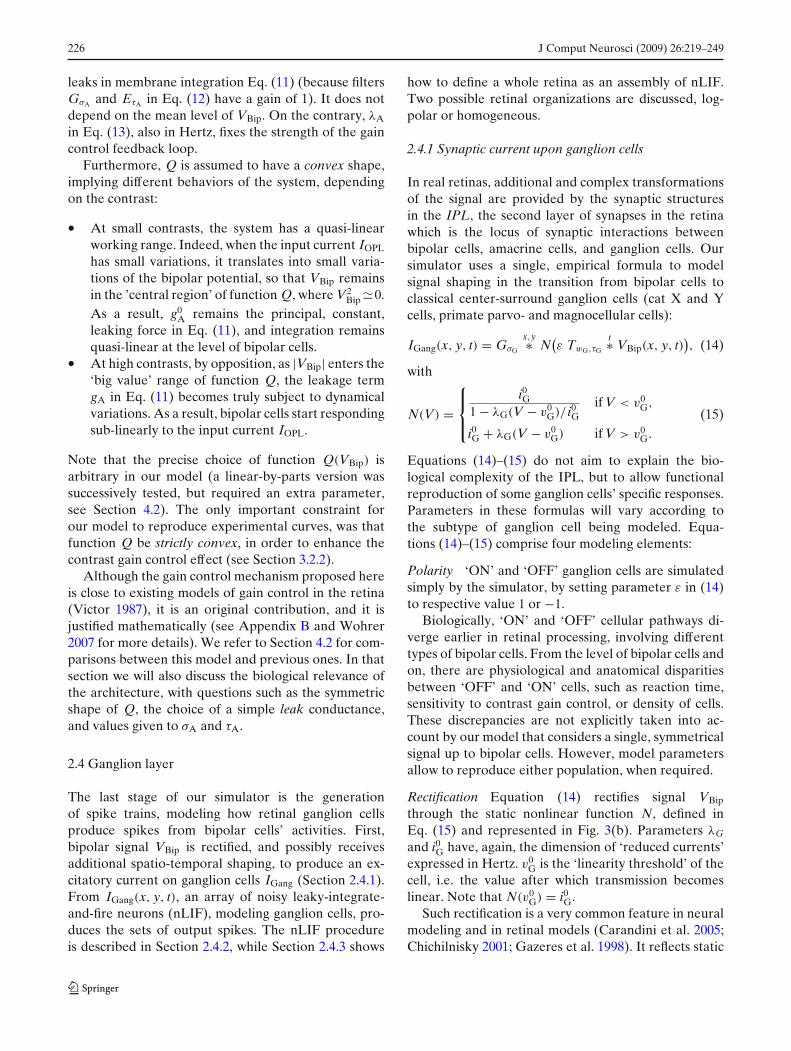
226 J Comput Neurosci (2009) 26:219–249
leaks in membrane integration Eq. (11) (because filtersGσA and EτA in Eq. (12) have a gain of 1). It does notdepend on the mean level of VBip. On the contrary, λA
in Eq. (13), also in Hertz, fixes the strength of the gaincontrol feedback loop.
Furthermore, Q is assumed to have a convex shape,implying different behaviors of the system, dependingon the contrast:
• At small contrasts, the system has a quasi-linearworking range. Indeed, when the input current IOPL
has small variations, it translates into small varia-tions of the bipolar potential, so that VBip remainsin the ’central region’ of function Q, where V2
Bip �0.As a result, g0
A remains the principal, constant,leaking force in Eq. (11), and integration remainsquasi-linear at the level of bipolar cells.
• At high contrasts, by opposition, as |VBip| enters the‘big value’ range of function Q, the leakage termgA in Eq. (11) becomes truly subject to dynamicalvariations. As a result, bipolar cells start respondingsub-linearly to the input current IOPL.
Note that the precise choice of function Q(VBip) isarbitrary in our model (a linear-by-parts version wassuccessively tested, but required an extra parameter,see Section 4.2). The only important constraint forour model to reproduce experimental curves, was thatfunction Q be strictly convex, in order to enhance thecontrast gain control effect (see Section 3.2.2).
Although the gain control mechanism proposed hereis close to existing models of gain control in the retina(Victor 1987), it is an original contribution, and it isjustified mathematically (see Appendix B and Wohrer2007 for more details). We refer to Section 4.2 for com-parisons between this model and previous ones. In thatsection we will also discuss the biological relevance ofthe architecture, with questions such as the symmetricshape of Q, the choice of a simple leak conductance,and values given to σA and τA.
2.4 Ganglion layer
The last stage of our simulator is the generationof spike trains, modeling how retinal ganglion cellsproduce spikes from bipolar cells’ activities. First,bipolar signal VBip is rectified, and possibly receivesadditional spatio-temporal shaping, to produce an ex-citatory current on ganglion cells IGang (Section 2.4.1).From IGang(x, y, t), an array of noisy leaky-integrate-and-fire neurons (nLIF), modeling ganglion cells, pro-duces the sets of output spikes. The nLIF procedureis described in Section 2.4.2, while Section 2.4.3 shows
how to define a whole retina as an assembly of nLIF.Two possible retinal organizations are discussed, log-polar or homogeneous.
2.4.1 Synaptic current upon ganglion cells
In real retinas, additional and complex transformationsof the signal are provided by the synaptic structuresin the IPL, the second layer of synapses in the retinawhich is the locus of synaptic interactions betweenbipolar cells, amacrine cells, and ganglion cells. Oursimulator uses a single, empirical formula to modelsignal shaping in the transition from bipolar cells toclassical center-surround ganglion cells (cat X and Ycells, primate parvo- and magnocellular cells):
IGang(x, y, t) = GσG
x,y∗ N(ε TwG,τG
t∗ VBip(x, y, t)), (14)
with
N(V) =
⎧⎪⎨
⎪⎩
i0G
1 − λG(V − v0G)/ i0
Gif V < v0
G,
i0G + λG(V − v0
G) if V > v0G.
(15)
Equations (14)–(15) do not aim to explain the bio-logical complexity of the IPL, but to allow functionalreproduction of some ganglion cells’ specific responses.Parameters in these formulas will vary according tothe subtype of ganglion cell being modeled. Equa-tions (14)–(15) comprise four modeling elements:
Polarity ‘ON’ and ‘OFF’ ganglion cells are simulatedsimply by the simulator, by setting parameter ε in (14)to respective value 1 or −1.
Biologically, ‘ON’ and ‘OFF’ cellular pathways di-verge earlier in retinal processing, involving differenttypes of bipolar cells. From the level of bipolar cells andon, there are physiological and anatomical disparitiesbetween ‘OFF’ and ‘ON’ cells, such as reaction time,sensitivity to contrast gain control, or density of cells.These discrepancies are not explicitly taken into ac-count by our model that considers a single, symmetricalsignal up to bipolar cells. However, model parametersallow to reproduce either population, when required.
Rectification Equation (14) rectifies signal VBip
through the static nonlinear function N, defined inEq. (15) and represented in Fig. 3(b). Parameters λG
and i0G have, again, the dimension of ‘reduced currents’
expressed in Hertz. v0G is the ‘linearity threshold’ of the
cell, i.e. the value after which transmission becomeslinear. Note that N(v0
G) = i0G.
Such rectification is a very common feature in neuralmodeling and in retinal models (Carandini et al. 2005;Chichilnisky 2001; Gazeres et al. 1998). It reflects static
J Comput Neurosci (2009) 26:219–249 227
nonlinearities observed experimentally in the retina(Chichilnisky 2001; Kim and Rieke 2001; Baccus andMeister 2002), e.g., through LN analysis of retinal cells(see Section 3.2.3 for the definition of LN analysis).Biologically, static nonlinearities in signal transmissioncan occur for different reasons: saturations, synaptictransmissions, etc. Eq. (15) defines a smooth rectifica-tion with a shape close to experimental curves observedwhen performing an LN Analysis (see Section 3.2.3).
Additional transient The temporal filter TwG,τG allowsto control how much the simulated ganglion cells arephasic or tonic. The tonic-phasic opposition is a generalconcept in physiology that can be described in sim-ple words: “A tonic process is one that continues forsome time or indefinitely after being initiated, while aphasic process is one that shuts down quickly” (Erwin2004). For primate Magnocellular cells or cat Y cells,response to a constant stimulation shuts down quicklyafter one or two hundreds of milliseconds, requiring theuse of a transient weight wG close to 1. By opposition,for our simulations of cat X cells, the supplementarytransient was fixed at an intermediate balance (wG =0.7) in order to reproduce correct Wiener kernels inSection 3.2.2, and correct responses to gratings in 3.2.1.
There are several plausible biological explanationsfor the transient properties intrinsic to ganglion cells.Likely, one main reason is the existence of specificamacrine cells in the IPL that were found to cut the re-sponses of ganglion cells (Nirenberg and Meister 1997;Masland 2001; Kolb et al. 2001), whether through afeedback to bipolar cells, whether by direct inhibitionon ganglion cells.
Locating this transient before the static nonlinearityN is a convenient, empirical choice. First, it providesbetter reproduction of Y cells’ spatial nonlinearity (seenext paragraph and Section 3.2.1) by creating fullyband-pass units before the rectification and pooling.Second, it allows undershoots possibly generated by thetransient filter TwG,τG to be attenuated by the compres-sion N.
Additional pooling The spatial filter GσG aims at re-producing a typical nonlinear effect observed in cat Ycells (Enroth-Cugell and Robson 1966) (an illustrationcan be seen in our simulations of Section 3.2.1). Thesimplest explanation of this spatial nonlinearity is aspatial pooling that would occur after the synaptic recti-fication onto these ganglion cells. This explanation, firstproposed by Hochstein and Shapley (1976), is at thebase of the Freeman and Enroth-Cugell model for Y-type cells (Enroth-Cugell and Freeman 1987). Further-more, the biological basis was justified experimentally
(Demb et al. 2001; Kolb et al. 2001): The spread ofthe dendritic tree of Y-type cells is large enough tosignificantly average the synaptic input from bipolarcells over a consequent spatial extent.
Remark: Other explanations have been proposed toaccount for the nonlinearity of Y cells. For example,Hennig et al. (2002) find that part of the nonlinearitymight be due to the spatial integration by Y cells ofa temporal nonlinearity due to phototransduction. Al-though they propose a different model, their work alsoneeds a wide spatial pooling at the level of Y cells.
2.4.2 Spike generation in ganglion cells
This section is about the transformation of the con-tinuous signal IGang(x, y, t) into discrete sets of spiketrains. Let us consider N ganglion cells Cn (n = 1 . . . N)paving the retinal space (see Section 2.4.3 for theirrepartition and parameters) and let us denote by Vn
the potential of cell number n (n = 1 . . . N) centered atposition (xn, yn).
Our simulator simply generates the output of cell Cn
with a standard nLIF model:
⎧⎪⎪⎪⎪⎪⎪⎪⎪⎪⎨
⎪⎪⎪⎪⎪⎪⎪⎪⎪⎩
dVn
dt= IGang(xn, yn, t) − gLVn(t) + ηv(t), (16)
Spike when threshold is reached: Vn(tspk) = 1,
Refractory period: Vn(t) = 0 while t < tspk + ηrefr,
and (16) again,
where ηv(t) and ηrefr are two noise sources that canbe added to the spike generation process in order toreproduce the trial-to-trial variability of real ganglioncells, following the experimental results of Keat et al.(2001). ηv(t) is taken as a Brownian movement that hasthe dimension of a current. Integration of this currentthrough Eq. (16) is equivalent to adding to Vn(t) aGaussian auto-correlated process with time constant1/gL (typically, 20 ms), and variance σv . The ampli-tude of ηv(t) is chosen for σv to be around 0.1. ηrefr
is a stochastic absolute refractory period that is ran-domly chosen after each spike, following a normal law,typically N (3 ms,1 ms).
Note that spike generation is the only source ofnoise in our model, following the model of (Keatet al. 2001) for trial-to-trial variability in ganglion spiketrains. Recent findings (Dhingra and Smith 2004) have

228 J Comput Neurosci (2009) 26:219–249
confirmed that the spiking mechanism is an importantcontribution to the overall noise in retinal processing.
Remark: ISI distributions – Poisson or not Poisson?Measuring inter-spike intervals (ISIs) is a commonway of estimating the nature of the spike generationprocess. In real experiments, it is observed that reti-nal spike trains have less variability than a simplePoisson emission process (see e.g. Kara et al. 2000 forreferences), at least during the periods of high firingactivity (Hartveit and Heggelund 1994). The coefficientof variation of retinal spike trains (CV, defined as theratio between standard deviation and mean of the ISIhistogram) was generally measured smaller than one,meaning less variability than a Poisson process. As aresult, the spiking procedure has often been modeledthrough Gamma renewal processes, which can be seenas a generalization of Poisson processes, but with acontrollable CV (see e.g. Gazeres 1998 for references).
However, in Poisson as in Gamma processes, the CVis constant whatever the input current. By opposition,some studies (Hartveit and Heggelund 1994) find thatthe CV of retinal spike trains depends on the intensityof the spike emission: retinal spikes become more pre-dictable (CV decreases) during periods of high spikingactivity. To account for this reality, Gazeres et al. (1998)propose a model which switches dynamically betweena Poisson and a Gamma procedure with smaller CV,according to the values of the generating signal. Butprecise fitting of this model to biological data has notbeen done to our knowledge.
By comparison, the nLIF model that we use herewas experimentally proved to successfully predict theoccurrences of retinal spikes, in different species (Keatet al. 2001), yielding typical noise parameters that wecould use in our model. An nLIF model has also beenused to reproduce spike variability in the LGN (Lesicaand Stanley 2004). The simulated ISIs in our nLIFmodel resemble those of a Gamma process, with a CVdependent on the amount of noise added in the spikegeneration through noise sources ηv and ηrefr (personalexperimentation).
However, we have not yet well established the be-havior of the CV with input current for this nLIFmodel. From first experimentation, the CVs displaysome variability with input current (unlike a Gammaprocess), but not sufficiently compared to real cells.And, indeed, some experimental reproductions by oursimulator suggested that our emitted spikes are proba-bly too deterministic at low contrast. The spiking nLIFmodel may be enhanced in the future by adding adynamical variation on the intensity of ηv , depending
on the instantaneous intensity of the generatingcurrent.
Remark: Spike correlations between neighboring cells.Other experiments revealed a stimulus-dependentsynchrony between the spikes of neighboring cells(Neuenschwander and Singer 1996) (also, see Kenyonet al. 2004; Kenyon and Marshak 1998 for a modelof this synchrony based on feedbacks from long- andshort-range amacrine cells). Such input-driven syn-chrony is not taken into account yet by the simulator,but we consider it as an interesting future extension.
2.4.3 Ganglion cell sampling configurations
The whole model presented above holds when model-ing a small region of the retina, in which the densityof retinal cells can be considered uniform. In that case,all filtering scales and parameters are constant and donot depend on the spatial position of each cell. Oursimulation software can easily handle such a uniformdistribution of cells.
However, mammalian (and especially primate) reti-nas taken as a whole are not uniform at all. Densityof cells and filtering scales depend on the positionconsidered in the retina. One needs to distinguish thefovea in the center, from the surround of the visualfield where precision is less. A simple way is to definea scaling function, that describes at the same time thelocal density of cells and the spatial scales of filtering inthe different regions of the retina.
Our simulator implements a radial and isotropic den-sity function that depends on the distance r from thecenter of the retina. We define a one-dimensional log-polar scaling function s(r) as
s(r) ={
1 if r < R0,
1/(1 + K(r − R0)) if r > R0,(17)
where R0 is the size of the fovea and K is the speedof density decrease outside of the fovea. When K =1/R0, this amounts to a traditional log-polar scaling.The density of cells in a given region of the retina ateccentricity r is then given by d0 s(r)2, d0 being the2d-density of cells in the fovea. Conversely, all spatialfiltering scales of the model presented before (σC, σS,σAm, σGang) scale with s(r)−1.
The choice of such a scaling function is biologicallyjustified: Dendritic trees for primate ganglion cells haveexperimentally been found to scale with a positivepower of r, between r0.7 and r according to the type ofcell (Dacey and Petersen 1992).
J Comput Neurosci (2009) 26:219–249 229
3 Results
3.1 Virtual Retina customization
The software Virtual Retina implements the model pre-sented in this article, with the following characteristics:
Possibility of large-scale simulations Up to 100,000spiking cells can be simulated in a reasonable time(speed of around 1/100 real time).
XML definition file All parameters for the differentstages of the model are defined in a single customizableXML file.
Two possible density functions First option is a uni-form, square array of cells, associated to a uniformdensity function. In that case, all spatial filtering scalesof the model (σC, σS, σAm, σGang) are constant through-out the whole image, and the corresponding Gaussianfilters Gσ (x, y) are implemented thanks to traditionalrecursive Deriche filters. Second option is a sampling ofganglion cells along concentric circles, associated to theradial scaling s(r) in Eq. (17). In that case, the Gaussianfilters Gσ (x, y) have different scales according to thelocation in the retina. They are implemented thanksto a recursive filtering with inhomogeneous recursivecoefficients, an approximation proposed in Tan et al.(2003) that leads to a significant gain in computationalspeed.
Fixation microsaccades Finally, the software allows toinclude a simple random microsaccades generator atthe input of the retina, to account for fixation eyemovements, as inspired from Martinez-Conde et al.(2004).
To provide a better fit to the specific complexity re-quired by potential users, we wished to build a modularsoftware, that allows some liberty in the choice of theunderlying model. Virtual Retina needs an XML filethat defines all the parameters of the retina chosen forthe simulation. This XML file is customizable: Eachfeature, as defined in this article, corresponds to its ownXML node, which can be present or not in the XML de-finition file. One example file is shown in Appendix C.
As a result, the output of the software can consistof spikes or continuous maps, the contrast gain controlcan be present or not, the retina can follow a log-polar scheme or a uniform scheme, etc. This flexibilityrequired important efforts in the conception of thesoftware (Wohrer 2008a).
In the on-line web service, a dedicated page assistsusers in customizing their own XML file.
3.2 Physiological reproductions
In this section we test our simulator on classical physio-logical experiments, led on single ganglion cells. Theseexperiments, with various protocols, demonstrate thatour underlying model induces linear kernels close tothose measured physiologically, and can also accountfor two typical nonlinear effects: Contrast gain controland spatial nonlinearity of Y-type ganglion cells.
A first experiment (Section 3.2.1) is devoted toreproduction of the physiological difference betweenX and Y- type cells. The two following experiments(Sections 3.2.2 and 3.2.3) are devoted to the phenom-enon of contrast gain control in the retina. We showthat our gain control loop Eqs. (11)–(13), along withthe rest of the model, reproduces qualitatively the dy-namical changes in retinal filtering linked to the averagelevel of contrast.
3.2.1 X and Y cell responses to grating apparitions
Description of the experiment. Grating apparitions area classical stimulus when experimenting on the low-level visual pathway. We reproduce here one of the firstrecordings of that kind, on cat ganglion cells in 1966by Enroth-Cugell and Robson (1966), which led to thedistinction between cat X type and Y type cells.
Cat ‘OFF’ ganglion cells are presented with the al-ternation of a static grating and a uniform screen ofsame luminance, at a frequency of about 0.5 Hz, andtheir spiking output is measured extracellularly. Theexperiment is repeated for different spatial phases ofthe grating, so as to test the summing properties ofthe cells’ receptive fields. Typical responses (averagedinstantaneous frequencies) for a X cell and a Y cell arepresented in Fig. 4.
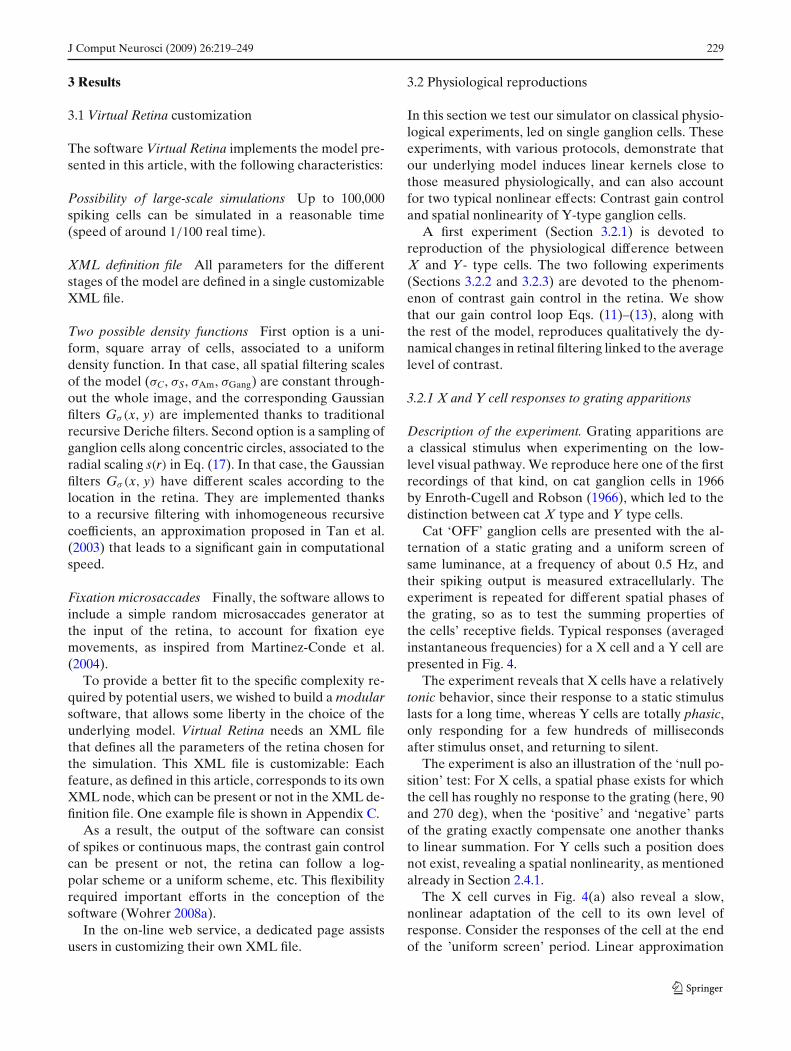
The experiment reveals that X cells have a relativelytonic behavior, since their response to a static stimuluslasts for a long time, whereas Y cells are totally phasic,only responding for a few hundreds of millisecondsafter stimulus onset, and returning to silent.
The experiment is also an illustration of the ‘null po-sition’ test: For X cells, a spatial phase exists for whichthe cell has roughly no response to the grating (here, 90and 270 deg), when the ‘positive’ and ‘negative’ partsof the grating exactly compensate one another thanksto linear summation. For Y cells such a position doesnot exist, revealing a spatial nonlinearity, as mentionedalready in Section 2.4.1.
The X cell curves in Fig. 4(a) also reveal a slow,nonlinear adaptation of the cell to its own level ofresponse. Consider the responses of the cell at the endof the ’uniform screen’ period. Linear approximation
230 J Comput Neurosci (2009) 26:219–249
Fig. 4 Response of catOFF-center ganglion cellsto the disappearance andreappearance of a sinusoidalgrating with different spatialoffsets, reproduced fromEnroth-Cugell and Robson(1966). (a): typical X-typeganglion cell. (b): typicalY-type ganglion cell (seedetails in the text). Gratingspatial frequencies of 0.13deg−1 (a) and 0.16 deg−1
(b). Mean luminance 16cd/m2, grating contrast of 0.32
(a) (b)
would predict similar levels of response in the fourexperimental conditions, since the uniform screen hasalready been on for a whole second, which exceeds thelatency of the cell’s linear response.
However, real cell responses at the end of the ‘uni-form screen’ period are bigger in the experiment withthe ‘0 deg’ grating, and lower with the ‘180 deg’ grating.This can be explained by a slow adaptation of the cell’sgain to its global level of response, which is strongerin the ‘180 deg’ experiment because the cell respondsstrongly when the grating is on.
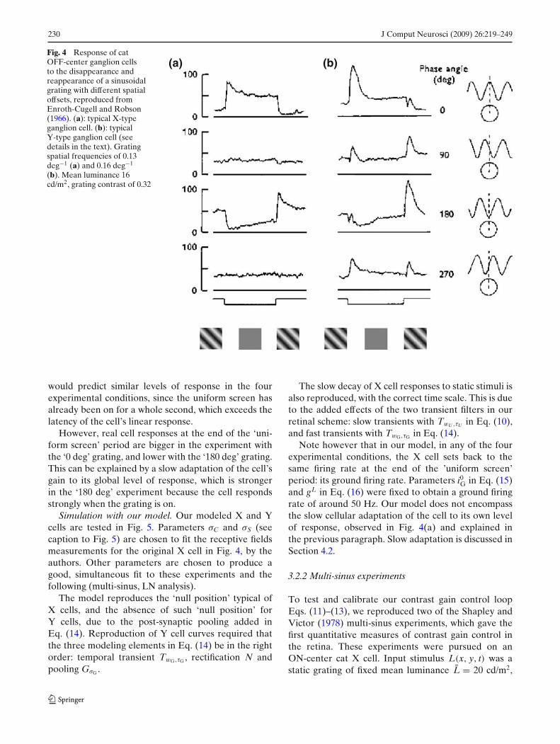
Simulation with our model. Our modeled X and Ycells are tested in Fig. 5. Parameters σC and σS (seecaption to Fig. 5) are chosen to fit the receptive fieldsmeasurements for the original X cell in Fig. 4, by theauthors. Other parameters are chosen to produce agood, simultaneous fit to these experiments and thefollowing (multi-sinus, LN analysis).
The model reproduces the ‘null position’ typical ofX cells, and the absence of such ‘null position’ forY cells, due to the post-synaptic pooling added inEq. (14). Reproduction of Y cell curves required thatthe three modeling elements in Eq. (14) be in the rightorder: temporal transient TwG,τG , rectification N andpooling GσG .
The slow decay of X cell responses to static stimuli isalso reproduced, with the correct time scale. This is dueto the added effects of the two transient filters in ourretinal scheme: slow transients with TwU ,τU in Eq. (10),and fast transients with TwG,τG in Eq. (14).
Note however that in our model, in any of the fourexperimental conditions, the X cell sets back to thesame firing rate at the end of the ’uniform screen’period: its ground firing rate. Parameters i0
G in Eq. (15)and gL in Eq. (16) were fixed to obtain a ground firingrate of around 50 Hz. Our model does not encompassthe slow cellular adaptation of the cell to its own levelof response, observed in Fig. 4(a) and explained inthe previous paragraph. Slow adaptation is discussed inSection 4.2.
3.2.2 Multi-sinus experiments
To test and calibrate our contrast gain control loopEqs. (11)–(13), we reproduced two of the Shapley andVictor (1978) multi-sinus experiments, which gave thefirst quantitative measures of contrast gain control inthe retina. These experiments were pursued on anON-center cat X cell. Input stimulus L(x, y, t) was astatic grating of fixed mean luminance L̄ = 20 cd/m2,
J Comput Neurosci (2009) 26:219–249 231
(b)(a)
Fig. 5 Reproduction of the experiments in Fig. 4 by our retinamodel. (a:) X cell model, (b:) Y cell model. Average firing ratesgenerated from 80 trials with noise in the spike generation. Testgrating: Normalized mean luminance of 0.5, contrast 0.32, spatialfrequency of 0.13 deg−1. OPL parameters: Center, σC = 0.88 deg,τC = 10 ms, nC = 2. Surround, σS = 2.35 deg, τS = 10 ms. Slowlinear transient, wU = 0.8, τU = 100 ms. Global amplification,
λOPL = 1000 Hz per normalized luminance unit. Gain controlparameters: g0
A = 5 Hz, λA = 50 Hz, τA = 5 ms, σA = 2.5 deg.X cell parameters: IPL transients, wG = 0.7, τG = 20 ms. Synaptictransmission, σG = 0, λG = 150 Hz, v0
G = 0, i0G = 80 Hz. Y cellparameters: IPL transients, wG = 1, τG = 50 ms. Synaptic trans-mission, σG = 1.8 deg, λG = 300 Hz, v0
G = 0, i0G = 80 Hz. Spikegeneration: gL = 50 Hz, σv=0.2, ηrefr ∼ N (3 ms, 1 ms)
temporally modulated by a sum of sinusoids withadjustable contrasts:
L(x, y, t) = L̄
(1 + Gr(x, y)
8∑
i=1
ci sin(ξit)
), (18)
where Gr(x, y) is a sinusoidal grating function withnormalized amplitude (between −1 and 1). The ξi area set of eight temporal frequencies that logarithmicallyspan the frequency range from about 0.2 to 32 Hz,respectively associated to contrast strengths ci.
Recordings were made for different distributions ofthe ci. For each recording, the cell’s output firing ratewas Fourier-analyzed at each of the input frequenciesξi, thus yielding a set of eight amplitudes and eightphases. This set provided a measure for the linearkernel (first-order Wiener kernel) that best fits the cell’sresponse, in the given contrast conditions.
Influence of the mean level of contrast
Description of the experiment. This first experimentmeasures how the mean level of contrast changes thebest-fitting first-order Wiener kernel for the cell. Theci are all fixed at the same value ci = c, global level ofcontrast for the stimulus. The experiment is repeatedfor four values of contrast, c being doubled each time.
Remark When ∀i, ci = c, the temporal part of signalEq. (18) is related to a pink noise stimulus (with sim-ilar power in each frequency octave). However, thespectrum of Eq. (18) is concentrated on eight discretevalues, unlike a real pink noise.
The resulting amplitude and phase diagrams for thecell’s output, represented in Fig. 6(a) and (b), revealdeviations from linearity: If the ganglion cell responded

232 J Comput Neurosci (2009) 26:219–249
Fig. 6 Contrast gain controlin a cat ON-center X ganglioncell, reproduced fromShapley and Victor (1978).(a and b): response tomulti-sinus stimuli ofdifferent contrasts c (sampleinput signal depicted in panelc-1). Amplitude curves (a)reveal under-linearity at lowtemporal frequencies. Phasecurves (b) reveal timeadvance for high contrasts(see text). Successively, c was0.0125 ( �), 0.025 (�), 0.05(�) and 0.1 ( �).(d): Strength of the gaincontrol effect depends on thedominant frequency ξi0present in the input (stimuliwith a carrier frequency ξi0 , asdepicted in Panel c-2). Thethree curves representindicators φ5(ξi0 ) ( �), φ6(ξi0 )
(�) and φ7(ξi0 ) (�) whichmeasure the strength of thegain control (see text).Frequencies that elicit themost gain control areξi0 =3–10 Hz
32103.20.320.1 1 32103.20.320.1 1
32103.20.320.1 1
Frequency (Hz) Frequency (Hz)
(d)
(b)(a)
− 1
(c)
− 2
10
0.32
1
3.2
32 0.5
0
− 0.5
− 1.5
~c
(1)
(2)
Am
plit
ude (
spk/s
)
Phase (
ra
d)
Phase s
hift (
r
ad)
0
0.1
0.2
0.3
0.4
time (s) Carrier frequency (Hz)
Am
plit
ude (
lum
.)
ππ
linearly to its input, the modulations in its responsewould simply be proportional to c. Successive ampli-tude curves in Fig. 6(a) would be parallel, spaced bylog(2) as contrast is doubled, and all phase curves inFig. 6(b) would superimpose, since the phase portraitdepends only on the nature of the linear filter.
Instead, the cell responds under-linearly to contrastat low temporal frequencies, where successive ampli-tude curves are spaced by less than log(2). In the phaseportrait, strong contrasts induce a phase-advance ofthe response (phase curve shifted upwards), meaningthat the cell responds faster at high contrasts. Ampli-tude compression at low frequencies and phase ad-vance are the dual mark of the contrast gain controleffect, as defined by Shapley and Victor. The authorsfound the two phenomena to be highly correlated intheir experiments, probably resulting from a commonmechanism.
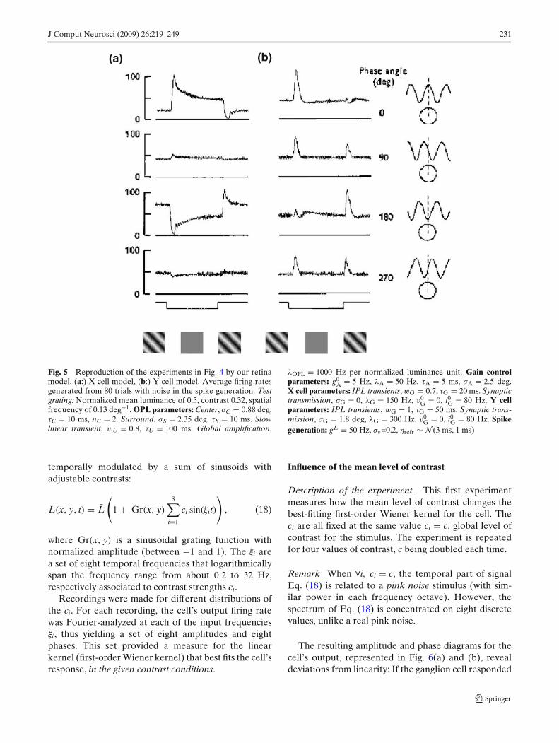
Simulation with our model Reproduction by ourmodel is shown in Fig. 7(a) and (b). The model repro-duces the typical time advance of ganglion responses athigh contrasts (Fig. 7(b)). This is because conductancegA in Eq. (11) determines the time constant of theresponse of bipolar cells, and that the mean level of gA,
dependent on the average of V2Bip, is a growing value of
contrast.Similarly, the under-linearity of response amplitudes
with contrast is also observed (successive curves spacedby less than log(2) in Fig. 7(a)). This is because gA inEq. (11) increases the leak in the bipolar membrane,and thus lowers the linear gain of bipolar transmissionin the case of high input contrast.
According to the preceding intuitive explanation,any shunting feedback loop necessarily implies a phaseadvance and an amplitude compression, and thus con-trast gain control. However, reproducing the exactshape of the kernel, and how it varies with contrast,required more specific features from our model.
First, the feedback loop Eqs. (11)–(13) is globally alow-pass setting, that can by no means reproduce theband-pass behavior observed in Fig. 6(a). The band-pass behavior in our model arises before the feedbackloop, through filter TwU ,τU in Eq. (8) that accounts fortemporal transients in the first layers of the retina, andafter the feedback loop, through filter TwG,τG in Eq. (15)that accounts for temporal transients in the IPL.
Second, we found mandatory that function Q inEq. (13) be strictly convex with a flat zone aroundVBip = 0, in order to reproduce the pronounced change
J Comput Neurosci (2009) 26:219–249 233
Fig. 7 Reproduction of thegain control effect by a modelcat X cell. (a), (b) and (d)have same signification as inFig. 6 (including variouscurve markers).(c) represents the amplituderesponses for the model cellin the ‘carrier frequency’experiments (stimuli as inFig. 6(c-2)). Contrast gaincontrol is observed since the‘perturbation’ kernels do notsuperimpose (see text). Testgrating: mean luminance of0.5, 0.2 cycles/deg. X Cellparameters as in Fig. 5
32103.20.320.1 1 32103.20.320.1 1
32103.20.320.1 132103.20.320.1 1
10
0.32
1
3.2
32
Frequency (Hz) Frequency (Hz)
(d)
(b)(a)
(c)
0.5
Am
plit
ude (
spk/s
)
Phase (
ra
d)
Phase s
hift (
r
ad)
Am
plit
ude (
spk/s
)
Frequency (Hz) Carrier frequency (Hz)
0
− 0.5
− 1
− 1.5
− 2
32
3.2
10
0.32
1
0.2
0.1
0
ππ
in shape of the Wiener kernel between high andlow contrast. If simulations are done with Q(VBip) =λ|VBip|, we obtain parallel amplitude curves spaced byless than log(2): Contrast gain control is thus present,but we are unable to reproduce the specific transforma-tion of Wiener kernel shapes with contrast. The biolog-ical relevance of a strictly convex shape is discussed inSection 4.1.3.
Frequencies that induce contrast gain control
Description of the experiment. A second experimentwas crafted by Shapley and Victor (1978) to furtherinvestigate the origin of the gain control mechanism.Each input frequency ξi0 is successively chosen as a‘carrier’ frequency with ci0 = 0.2, while the other fre-quencies are added as perturbation terms: ci = 0.0125for i = i0 [see Eq. (18)]. Results are compared to a ‘lowcontrast’ test condition where ci = 0.0125 for all i.
For each carrier frequency ξi0 three phase advanceindicators φ5(ξi0), φ6(ξi0) and φ7(ξi0) are measured, re-spectively associated to assay frequencies ξ5 = 3.9, ξ6 =7.8 and ξ7 = 15.6 Hz. φ5(ξi0) is obtained by measuringoutput phase at the assay frequency ξ5 when ξi0 is thecarrier frequency, and subtracting the output phase at
ξ5 in the low-contrast test condition; similarly for φ6(ξi0)
and φ7(ξi0).Since contrast gain control can be measured by a
phase advance (previous paragraph), φ5(ξi0), φ6(ξi0) andφ7(ξi0) provide three indicators, hopefully highly corre-lated, of the strength of the gain control induced by ξi0 .
Figure 6(d) represents experimental measures forφ5(ξi0), φ6(ξi0) and φ7(ξi0). As predicted, the three indi-cators are highly correlated, consistently with the globaltime advance induced by contrast gain control. Phaseadvance is strongest when the carrier ξi0 is around3 − 10 Hz. This reveals that the underlying mecha-nism for the contrast gain control measured here has a‘band-pass’ sensitivity, being preferentially triggered bytemporal variations around 3 − 10 Hz.
Simulation with our model. The three measured phasedifferences φ5(ξi0), φ6(ξi0) and φ7(ξi0) for our model arerepresented in Fig. 7(d). We reproduce larger phaseadvances when the carrier frequency is in the range1 − 10 Hz. This is due to the temporal band-pass filterTwU ,τU in Eq. (8), that enhances the contributions offrequencies 1 − 10 Hz in the current IOPL which is fedto the gain control mechanism Eq. (11).
234 J Comput Neurosci (2009) 26:219–249
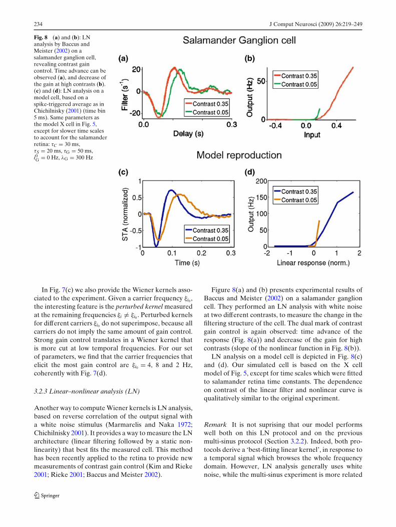
Fig. 8 (a) and (b): LNanalysis by Baccus andMeister (2002) on asalamander ganglion cell,revealing contrast gaincontrol. Time advance can beobserved (a), and decrease ofthe gain at high contrasts (b).(c) and (d): LN analysis on amodel cell, based on aspike-triggered average as inChichilnisky (2001) (time bin5 ms). Same parameters asthe model X cell in Fig. 5,except for slower time scalesto account for the salamanderretina: τC = 30 ms,τS = 20 ms, τG = 50 ms,i0G = 0 Hz, λG = 300 Hz
In Fig. 7(c) we also provide the Wiener kernels asso-ciated to the experiment. Given a carrier frequency ξi0 ,the interesting feature is the perturbed kernel measuredat the remaining frequencies ξi = ξi0 . Perturbed kernelsfor different carriers ξi0 do not superimpose, because allcarriers do not imply the same amount of gain control.Strong gain control translates in a Wiener kernel thatis more cut at low temporal frequencies. For our setof parameters, we find that the carrier frequencies thatelicit the most gain control are ξi0 = 4, 8 and 2 Hz,coherently with Fig. 7(d).
3.2.3 Linear–nonlinear analysis (LN)
Another way to compute Wiener kernels is LN analysis,based on reverse correlation of the output signal witha white noise stimulus (Marmarelis and Naka 1972;Chichilnisky 2001). It provides a way to measure the LNarchitecture (linear filtering followed by a static non-linearity) that best fits the measured cell. This methodhas been recently applied to the retina to provide newmeasurements of contrast gain control (Kim and Rieke2001; Rieke 2001; Baccus and Meister 2002).
Figure 8(a) and (b) presents experimental results ofBaccus and Meister (2002) on a salamander ganglioncell. They performed an LN analysis with white noiseat two different contrasts, to measure the change in thefiltering structure of the cell. The dual mark of contrastgain control is again observed: time advance of theresponse (Fig. 8(a)) and decrease of the gain for highcontrasts (slope of the nonlinear function in Fig. 8(b)).
LN analysis on a model cell is depicted in Fig. 8(c)and (d). Our simulated cell is based on the X cellmodel of Fig. 5, except for time scales which were fittedto salamander retina time constants. The dependenceon contrast of the linear filter and nonlinear curve isqualitatively similar to the original experiment.
Remark It is not suprising that our model performswell both on this LN protocol and on the previousmulti-sinus protocol (Section 3.2.2). Indeed, both pro-tocols derive a ‘best-fitting linear kernel’, in response toa temporal signal which browses the whole frequencydomain. However, LN analysis generally uses whitenoise, while the multi-sinus experiment is more related
J Comput Neurosci (2009) 26:219–249 235
to pink noise (preceding remark). As a result, the re-trieved kernels slightly differ between the two protocols(personal experimentation).
Remark Fast and slow contrast gain control Recentwork (Kim and Rieke 2001; Baccus and Meister 2002)has established that at least two contrast gain con-trol mechanisms are present in the retina with dif-ferent time scales: A fast, almost instantaneous gaincontrol mechanism, and a slower adaptation process(see discussion in Section 4.2). The multi-sinus exper-iments (Shapley and Victor 1978) in Fig. 6 use a pro-tocol which elicits both the slow and fast mechanisms.By opposition, the LN experiments of Baccus andMeister (2002) do discriminate fast from slow contrastgain control. The curves in Fig. 8(a) correspond specif-ically to their measure of the fast effect.
Our model only includes a fast gain control mech-anism. Figure 8(b) shows that our mechanism canqualitatively reproduce the fast component of contrastgain control. In turn, Fig. 7 shows that our mechanismis sufficient to qualitatively reproduce the multi-sinusexperiments, suggesting that biologically, fast contrast
gain control is mostly responsible for the change inshape of the kernels (a result confirmed in Baccus andMeister 2002).
3.3 Results on real images
To conclude our presentation of Virtual Retina, wepresent simulations on whole images and sequences.We do not study quantitatively any retinal feature inthis section: The article does not aim at such study, butat presenting a simulation tool. Rather, we illustratequalitatively how large-scale simulations allow to linka model architecture with its perceptual consequences.
First, as a general illustration of the software, wepresent the complete simulation of a retina on a mov-ing sequence, with spiking output and all intermedi-ate signals involved. Second, we focus on two specificelements of the model and how they relate to a percept.
3.3.1 Large-scale simulation of the model
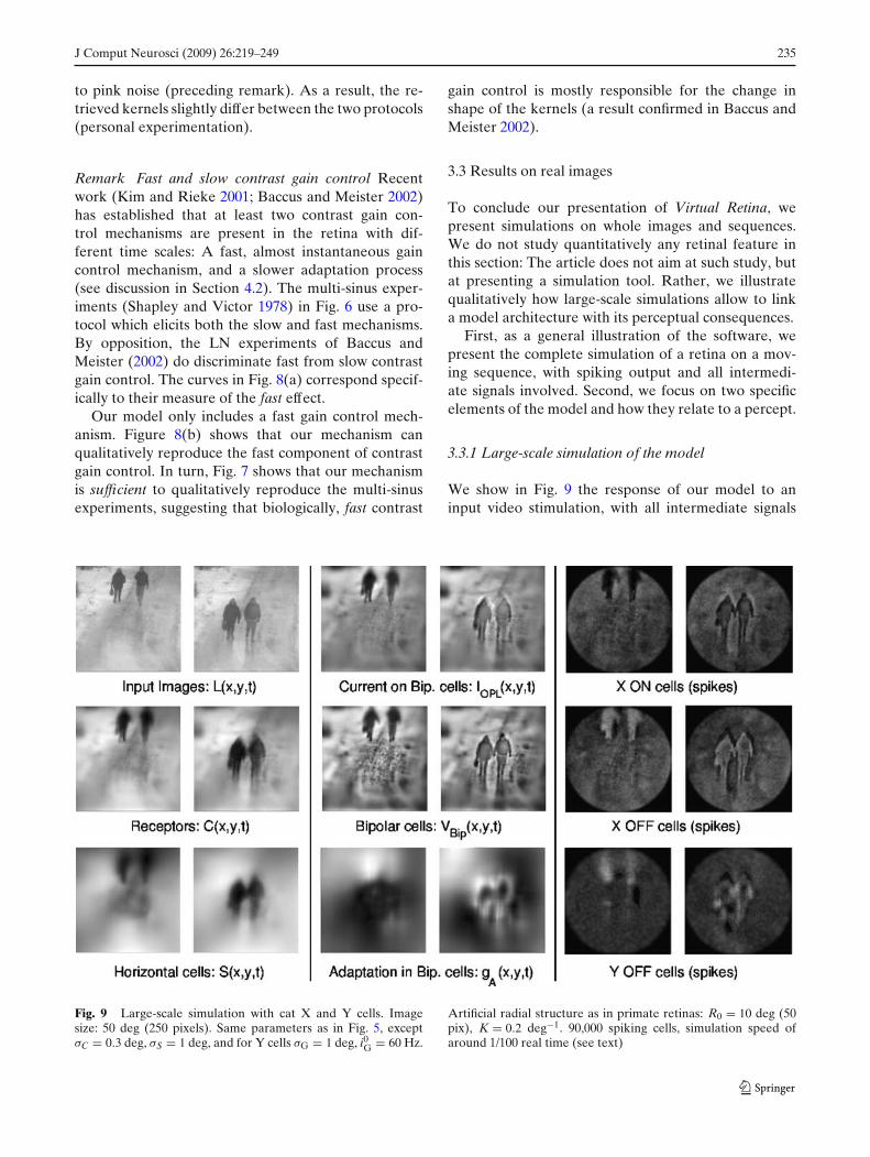
We show in Fig. 9 the response of our model to aninput video stimulation, with all intermediate signals
Fig. 9 Large-scale simulation with cat X and Y cells. Imagesize: 50 deg (250 pixels). Same parameters as in Fig. 5, exceptσC = 0.3 deg, σS = 1 deg, and for Y cells σG = 1 deg, i0G = 60 Hz.
Artificial radial structure as in primate retinas: R0 = 10 deg (50pix), K = 0.2 deg−1. 90,000 spiking cells, simulation speed ofaround 1/100 real time (see text)

236 J Comput Neurosci (2009) 26:219–249
represented at two instants of the simulation. To dis-play all possibilities of Virtual Retina, we chose a hybridretina, with cell properties being those of a cat retina(with X and Y cells), but that displays a radial structureas in a primate retina, with spatial precision maximumin the fovea, and decreasing towards the periphery.The simulated retina had a diameter of 50 deg, cor-responding to 250 pixels. The input sequence lasted1.4 s of ‘real time’, corresponding to 56 frames (eachframe shown for 25 ms). There were three ganglionlayers of 30,000 spiking cells each. On average, eachcell fired approximatively one spike per input frame.Total processing time was around 130 s (2 s per inputframe).
The foveated structure, ruled by sampling schemeEq. (17), can be observed on all retinal images (exceptfor the input light): The periphery is more blurred thanthe central zone.
Signals C, S and IOPL illustrate the properties of theOPL filter Eqs. (8)–(10): It is the difference of twolow-passed versions of the sequence, so it takes strongvalues on image edges and on moving zones. Its biggestresponse is thus located on the edges of the walkingcharacters.
Second column corresponds to layers IOPL, VBip andgA which are involved in the contrast gain controlscheme Eqs. (11)–(13). The contrast gain controlscheme enhances the linear contrast image IOPL toproduce VBip (which reveals better the details ofcontrast). This perceptual effect is detailed in thesequel.
Last column presents linear reconstructions from theoutput spike trains, respectively from X ON and OFFcells, and Y OFF cells. Each spike simply contributesto the reconstruction by adding a circular spot, whosediameter and intensity depend on the cell density inthis region of the retina, and whose temporal profile is adecreasing exponential of time constant 20 ms. Thus, areconstructed sequence displays in each pixel a quantityclose to the ‘instantaneous firing rate for a cell locatedat this pixel’.
The positive and negative parts of signal VBip arecoded respectively by ON and OFF ganglion cells. Ycells display a signal with less spatial precision than Xcells, because of the supplementary synaptic poolingGσG in Eqs. (14). Second, Y cells are only sensitiveto temporal changes, so they only detect the movingcharacters. This is obtained by making Y cells totallyphasic with wG = 1 in Eq. (14), and by lowering thespontaneous firing rate of Y cells, through parameteriG0 in Eq. (15).
3.3.2 Perceptual consequences of model architecture
Spiking pattern at image onset
It has long been known that the center-surroundarchitecture of ganglion cells produces preferentialresponses to spatial or temporal change. Many sub-sequent modeling has considered the retina – or atleast its center-surround ganglion cells pathway – as anedge detector. Here we suggest there could be anothereffect in the first milliseconds after image onset, due tothe biologically observed delay of surround signal w.r.tcenter signal (Enroth-Cugell et al. 1983; Bernadete andKaplan 1999).
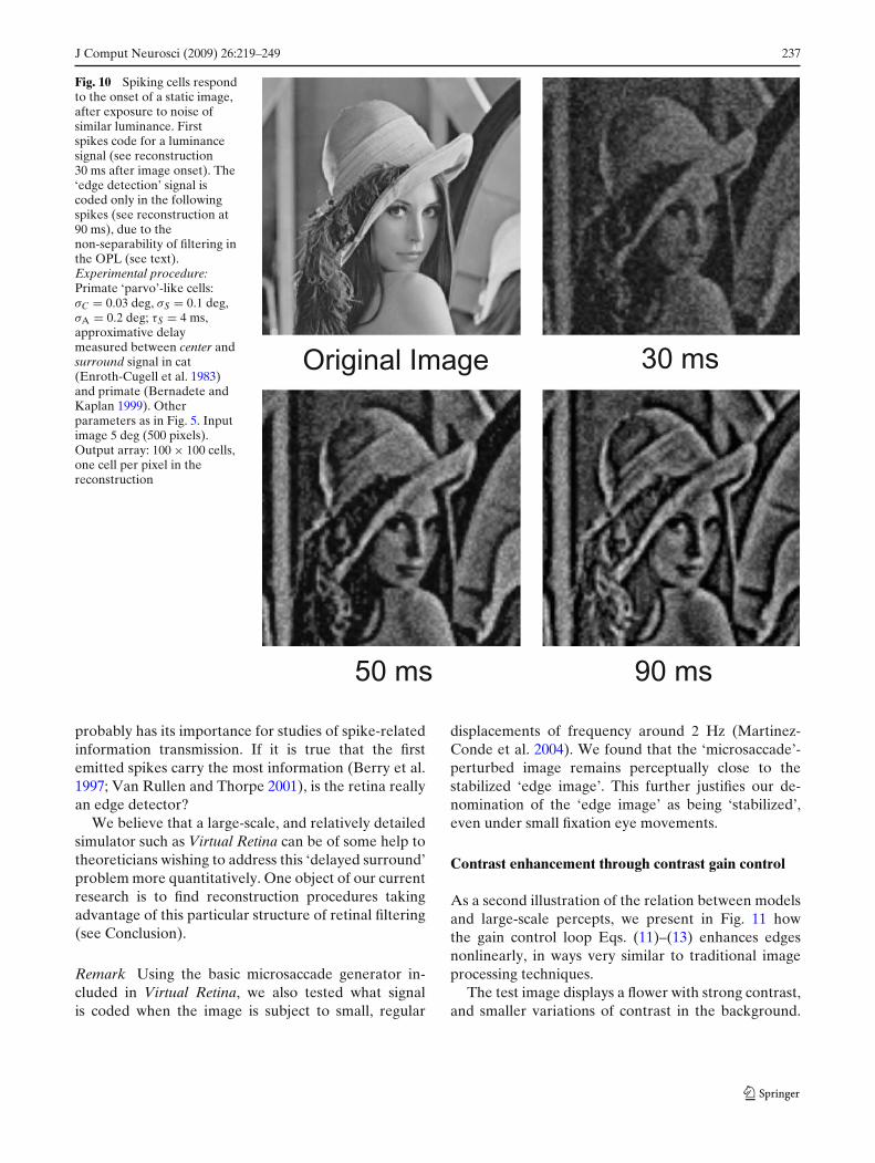
Figure 10 presents a reconstruction from the spikesemitted by a square array of primate ‘parvo’-like cells,after onset of a static image (one cell per pixel, eachspike adding an exponential contribution of latency15 ms). To produce plausible initial conditions, the cellsare previously exposed to Gaussian white noise of sameluminance as the forthcoming image.
The first spikes coding for the image (observablefrom around 20 ms after image onset) do not codefor image edges, but only for the center signal, simplyproportional to the input luminance: see reconstructionat time 30 ms. The following spikes progressively startcoding for image edges, as the delayed surround signal[Eq. (9)] catches up. In the reconstruction of Fig. 10,the transition is partly achieved at time 50 ms, totallyachieved at time 90 ms. It is surprising, but verified,that the small supplementary delay of surround (here,τS = 4 ms) has perceptual effects over several tens ofmilliseconds.
Very recent results (Gollisch and Meister 2008) havebrought experimental validation to this original pre-diction of our model. The authors reconstructed twoimages from the spike trains of a salamander fast OFFganglion cell in response to the onset of a static image:A first reconstruction image based on the latency of thefirst emitted spike (T), and a second image based onthe total number of spikes fired by the cell (N). Theirobservation, reproduced with our model (not shown),is that the ‘T’ image resembles the luminance inputprofile, while the ‘N’ image puts more accent on imageedges.
In our model, this subsequent ‘edge image’ is theequilibrium signal of the retina: It defines the ‘sta-bilized’ retinal output to the static image, after theinitial luminance transient at image onset (in real reti-nas, ‘stabilized’ is only an approximation, due to slowadaptation effects). But the initial ‘luminance transient’
J Comput Neurosci (2009) 26:219–249 237
Fig. 10 Spiking cells respondto the onset of a static image,after exposure to noise ofsimilar luminance. Firstspikes code for a luminancesignal (see reconstruction30 ms after image onset). The‘edge detection’ signal iscoded only in the followingspikes (see reconstruction at90 ms), due to thenon-separability of filtering inthe OPL (see text).Experimental procedure:Primate ‘parvo’-like cells:σC = 0.03 deg, σS = 0.1 deg,σA = 0.2 deg; τS = 4 ms,approximative delaymeasured between center andsurround signal in cat(Enroth-Cugell et al. 1983)and primate (Bernadete andKaplan 1999). Otherparameters as in Fig. 5. Inputimage 5 deg (500 pixels).Output array: 100 × 100 cells,one cell per pixel in thereconstruction
Original Image 30 ms
50 ms 90 ms
probably has its importance for studies of spike-relatedinformation transmission. If it is true that the firstemitted spikes carry the most information (Berry et al.1997; Van Rullen and Thorpe 2001), is the retina reallyan edge detector?
We believe that a large-scale, and relatively detailedsimulator such as Virtual Retina can be of some help totheoreticians wishing to address this ‘delayed surround’problem more quantitatively. One object of our currentresearch is to find reconstruction procedures takingadvantage of this particular structure of retinal filtering(see Conclusion).
Remark Using the basic microsaccade generator in-cluded in Virtual Retina, we also tested what signalis coded when the image is subject to small, regular
displacements of frequency around 2 Hz (Martinez-Conde et al. 2004). We found that the ‘microsaccade’-perturbed image remains perceptually close to thestabilized ‘edge image’. This further justifies our de-nomination of the ‘edge image’ as being ‘stabilized’,even under small fixation eye movements.
Contrast enhancement through contrast gain control
As a second illustration of the relation between modelsand large-scale percepts, we present in Fig. 11 howthe gain control loop Eqs. (11)–(13) enhances edgesnonlinearly, in ways very similar to traditional imageprocessing techniques.
The test image displays a flower with strong contrast,and smaller variations of contrast in the background.

238 J Comput Neurosci (2009) 26:219–249
Fig. 11 Perceptualcomparison between a linearoutput (b) and two versionsof the gain controlmechanism. When the gaincontrol is purely temporal(σA=0, panel c), it operatesas a point-by-point Gammatransform on the image.When the gain control isallowed to have a spatialextent (d), it operates like alocal histogram equalizationon the contrast image. (b) to(d) are equilibrium responses,after the initial transient atimage onset. Details andexperimental procedurein the text. Flower photocourtesy of Marcello Moisan(Moisan 2007)
We only consider here the equilibrium ‘edge image’ ofthe retina, rather than the initial ‘luminance transient’(as explained in the previous paragraph).
We compare the linear output of the retina IOPL
with two versions of VBip after contrast gain control.First version considers a purely temporal gain control

J Comput Neurosci (2009) 26:219–249 239
loop, with no spatial extent for the measure of contrastby gA(x, y, t) (through σA = 0 in Eq. (12)). A secondversion allows this spatial extent, with σA = 0.2 deg, avalue comparable to the extent of our surround signalσS = 0.1 deg. We study these two cases distinctly be-cause of the hypothetical nature of parameter σA in ourretinal model (see Discussion in Section 4.2).
To produce comparable results, the three resultingimages (IOPL(x, y) and the two VBip(x, y)) are normal-ized between −1 and 1, and passed through an adimen-sional rectification N as in Eq. (15) (with i0 = 0.3, λ = 1,v0 = 0, see Fig. 3(b)) modeling ganglion rectificationand spike generation.
Panel B presents the rectified version of IOPL(x, y),the linear response. In panels C and D, we presentthe interplay between the rectified nonlinear outputVBip(x, y) and the adapting conductance gA(x, y) thatproduced the nonlinear effect.
In the case of a purely temporal contrast gaincontrol (σA = 0, panel C), one can observe a re-equilibrating of the contrast levels, as compared tothe linear output (B). Intermediate contrast levels areenhanced as compared to high-contrast levels (see, e.g.,the small flower at the bottom left). Mathematically,when equilibrium is reached in Eqs. (11)–(13), one hasthe point-by-point relations gA(x, y) = Q(VBip(x, y)) =g0
A + λAVBip(x, y)2 and IOPL(x, y) = VBip(x, y)gA(x, y),so that the nonlinear output can simply be understoodas the static point-by-point compression
VBip(x, y) = L−1(IOPL(x, y)),
with L(V) = V(g0A + λAV2). So in this case (σA = 0, on
a static image), our gain control loop Eqs. (11)–(13)is close to a Gamma-transform (Gonzalez and Woods1992) on the original linear output.
In the case where contrast gain control mechanismincludes a spatial extent σA (panel D), the equilibriumbetween VBip(x, y) and gA(x, y) becomes dependent onthe spatial structure of the input image and there isno analytical expression. Intuitively, gA(x, y) providesa divisive effect on VBip(x, y) based on the contrast inthe neighborhood of (x, y), making VBip(x, y) a measureof contrast that is local rather than absolute. This en-hancement, which can be observed in the backgroundin D, is very close to a local histogram equalization (seeGonzalez and Woods (1992), chapter 3) on the linearcontrast image.
These results are another example of link betweenphysiological and perceptual features allowed by large-scale simulation. We wish to stress the qualitative na-ture of these perceptual results on contrast gain control.For example, one might argue that we humans do not
see such an enhanced contrast as that displayed inFig. 11(d). It should not be forgotten that the Midget(‘parvo’) pathway of primates, which is supposed tobe our primary source of precise form analysis, is verylittle subject to contrast gain control (Bernadete et al.1992). Besides, the problem of ‘double filtering’ (bythe software, and by our visual system) raises otherissues concerning what we see when looking at thereconstructions.
To conclude, note that physiological measurementssuch as those of Shapley and Victor 78 (Fig. 6(a))demonstrate that there is under-linearity to contrast incat ganglion cells, at least in specific spatio-temporalconditions (their experiments concerned sinusoidalstimulation, whereas here we simulate a totally staticimage). This necessarily implies a perceptual invari-ance, for all cells which display contrast gain control(cat cells, primate Parasol (‘magno’) cells): At least, astatic compression effect as in Fig. 11(c). Possibly, alocal equalization as in Fig. 11(d).
4 Discussion
4.1 Customizable simulation software
4.1.1 Combining large-scale and plausibility
The first aim of this article was to present VirtualRetina, a large-scale simulation software. Before go-ing into the details of the underlying retina model,we would like to stress the goals of this software: Toachieve at the same time large-scale simulation and arelative biological plausibility, with an adaptabledegree of complexity.
First of all, Virtual Retina is a large-scale simulator. Itaims at providing input to neuroscientists who need thislarge-scale factor: Motion detection tasks in a naturalscene, population coding by an assembly of spikingvisual neurons, information-theoretic calculations onnatural scenes. In this optic, it is being used by severalresearch teams of the FACETS5 European consortiumas input to detailed models of primary visual cortex(V1). It can also serve as a demonstration tool in aneducational framework.
As a large-scale simulator, we wished to reduce asmuch as possible the number of parameters used inthe underlying model. This explains the simple formtaken by our successive stages (OPL, contrast gaincontrol, IPL and ganglion cells), that discard manyeffects known to occur in real retinas.
5http://facets.kip.uni-heidelberg.de/.

240 J Comput Neurosci (2009) 26:219–249
At the same time, Virtual Retina intends to be aplausible simulator, that can provide output spike trainsreasonably close to those of real ganglion cells. Thereproduction of a number of experimental recordingsin Section 3 appeared a necessary step to prove theplausibility of the software.
As a plausible simulator, we wanted to keep spe-cific properties of retinal processing that are oftenignored by large-scale models. This includes: The non-separability of the OPL filter Eq. (10) that allows todetect both image edges and uniform flickering screens,the contrast gain control mechanism Eqs. (11)–(13)that provides invariance to contrast in natural scenes,and the trial-to-trial variability in the emission of spiketrains.
As a plausible simulator also, Virtual Retina uses anunderlying model mostly based on prior, state-of-the-art knowledge on the retina, experimental results aswell as models. Our goal was to reduce this state-of-the-art knowledge to formulations as simple as possible, forinclusion in the software. As an exception, our contrastgain control mechanism based on conductances is amore original contribution, although it also stronglyrelates to previous work. The mechanism is discussedin the next paragraph. Note that potential users lookingfor purely state-of-the-art simulation can easily dis-connect the contrast gain control stage, thanks to themodular nature of the software.
4.1.2 Subclasses of ganglion cells
In this section we shortly mention the different typesof ganglion cells reproducible by our simulator. Namesand classification of ganglion cells vary according tothe species considered, and to the classification medium(morphology or physiology) (Kolb et al. 2001; Masland2001). The goal of this section is not to review all types,
but just to give landmarks about retinal physiology andhow our simulator relates to them.
In the cat retina, X and Y cells are the most studiedtype. Both types of cells display a strong contrast gaincontrol (Shapley and Victor 1978), although the effectis stronger in Y cells. Y cells are more phasic, X cellsmore tonic. Finally, the response of Y cells cannot bemodeled by linear spatial summation. Our model canaccount for both X and Y types of cellular response (seeSection 3.2.1).
In the primate retina, Midget and Parasol cells havereceived the most attention. Midget cells are very pre-cise spatially (small receptive field) and code for red-green color oppositions. They are known to displaylittle contrast gain control (Kaplan and Bernadete2001). They are connected to the Parvocellular pathwayof the LGN, which is supposed to be in charge of preciseshape detection. Parasol cells have a wider receptivefield, are not sensitive to color but very sensitive tocontrast, and display a strong contrast gain controleffect. They are connected to the Magnocellular path-way of the LGN, which is supposed to be in chargeof movement detection and broad scene analysis. El-ements suggest that Midget cells constitute a new chan-nel of visual information possessed only by primates,whereas Parasol cells are a common feature shared withother mammals, being close for example to cat X andY cells (Kaplan and Bernadete 2001; Masland 2001).Following this hypothesis, Virtual Retina can reproduceprimate Parasol cells with efficiency. Midget cells canalso be reproduced in their achromatic features; butcolor oppositions are not handled yet by our model.Finally, as explained already, Virtual Retina handles thefoveated structure typical of primate retinas.
Table 2 summarizes plausible orders of magnitudefor the model parameters that must vary between catand primate retinas. Values for σC and σS are takenfrom the literature (Enroth-Cugell and Robson (1966)
Table 2 Model parameters that vary according to species (cat and primate) and pathway
Parameter Cat X Cat Y Parasol Midget
(*) σC (deg) 0.15–0.8 0.15–0.8 0.03–0.1 (fov) 0.03–0.1 (fov)(*) σS (deg) 0.8–6 0.8–6 0.2–0.7 (fov) 0.2–0.7 (fov)(?) σA (deg) 0–1.5 0–1.5 0–0.2 (fov) 0–0.2 (fov)(+) σG (deg) 0 1.5 0–0.15 (fov) 0 (fov)(+) λA (Hz) 50–100 50–100 50–100 0(+) g0
A (Hz) 5 5 5 50(+) wG 0.7 1 0.7–1 0.7(+) λG (Hz) 100 300 100–300 100
Plausible values for other parameters are in caption to Fig. 5. (*) Values taken from Enroth-Cugell and Robson (1966) (cat) and Cronerand Kaplan (1995), McMahon et al. (2000) (primate). (+) Values which provided good fit to the model. Most of these parameters haveequivalents in other retina models, with comparable values. (?) The adaptation spatial scale σA is a free parameter of the model, forwhich no data is available, only plausible orders of magnitude

J Comput Neurosci (2009) 26:219–249 241
for cat, Croner and Kaplan (1995), McMahon et al.(2000) for primate). Other parameters for cat cells areplausible orders of magnitude that provided good fitto data. Other parameters for primate cells are sugges-tions respecting the scaling from cat to primate retina,and the characteristics of primate cells explained in theabove paragraph: Parasol cells can behave like cat Xor Y cells, and Midget cells display no contrast gaincontrol.
Remark Many other types of ganglion cells have beenfound in the cat retina (W cells, Q cells. . . ) and inthe primate retina (such as small bi-stratified ganglioncells which code for Blue/Yellow color opponents)with functionalities more or less known (Masland 2001;Wohrer 2008b). Some are sensitive to illumination,others are tuned to directional movement (e.g., ON-OFF DS cells in rabbit retina), etc. Our model doesnot intend to reproduce these other subtypes, althoughwe believe that for some of them, modeling is relativelystraightforward from what is presented in this article.
4.1.3 Temporal transients and adaptation in the model
‘Adaptation’ is a word widely used in neurophysiology,that can convey various meanings. When presentingour model, we restricted this word to the descriptionof nonlinear effects in retinal filtering. Conversely, werather used the word ‘transient’ to define the temporalhigh-pass stages that we modeled through linear filters.Using this terminology, our simulator uses two lineartransient filters TwU ,τU and TwG,τG , and one contrastadaptation stage with the feedback loop Eqs. (11)–(13). We designed the feedback loop Eqs. (11)–(13)as a purely low-pass stage, by associating the adaptingconductance gA to a null Nernst potential. As a result,only the two linear filters TwU ,τU and TwG,τG are incharge of temporal shaping in the system.
Our adaptation scheme to contrast is discussed inSection 4.2. We wish to stress that this scheme onlyaims to reproduce fast gain control adaptation. Recentworks (Baccus and Meister 2002; Kim and Rieke 2001)have revealed a second mechanism of gain control, ona much slower time scale. This secondary gain controlenters the family of slow adaptation mechanisms inneurons, that we have not discussed nor included inour simulator. Likely, this slow adaptation is presentsimultaneously at different biological locations, bothpre- and post-synaptically to ganglion cells.
In the salamander, Kim and Rieke (2003, 2001) findthat slow contrast gain control could be accounted
for by a slow inactivation of Na+ currents due tospike generation in the ganglion cells. In mammalianretinas, some studies (Solomon et al. (2004) in pri-mate) also suggest that a large part of slow con-trast adaptation arises directly in ganglion cells, whileothers (Manookin and Demb (2006) in guinea pig)suggest that slow adaptation is mostly presynaptic tothe ganglion cells, because currents directly injected inganglion cells induce less slow adaptation.
For the moment, Virtual Retina ignores slow adap-tation, although a very experimental spike-frequencyadaptation scheme is available in the source code. Notethat if a slow adaptation was implemented in the model(spike-frequency adaptation or other), it would allowto account for the nonlinear variations of cat X cellsin response to a uniform screen, according to theirmean level of activity during the current stimulation(Section 3.2.1 and Fig. 4(a)).
As for linear filters TwU ,τU in Eq. (8) and TwG,τG inEq. (14), they must be seen as a functionally convenientchoice to reproduce band-pass behaviors in the retina.Their respective biological locations and time scales(100 ms for TwU ,τU versus 10 − 30 ms for TwG,τG ) do notintend to reproduce physiology with precision.
TwU ,τU in Eq. (8) can be associated to different phys-iological meanings: First, it is a crude approximationof the intrinsic undershoot occurring in cone photo-transduction in the time scales of a few hundreds ofmilliseconds (Schnapf et al. 1990). At the same time,it provides a very simple linear equivalent to slow cel-lular adaptation described in the previous paragraph.Finally, it serves as a way to correctly enhance the1 − 10 Hz frequency range before application of thecontrast gain control stage (see Section 3.2.2 andFig. 6(d)).
By opposition, TwG,τG in Eq. (14) is rather associatedto fast transients which occur later in retinal process-ing due to retinal connectivity. It accounts mostlyfor amacrine cells that provide a strong inhibition onsome bipolar cells and/or ganglion cells at the level ofsynapses in the IPL. TwG,τG is the processing step wherewe can fix the balance between tonic and phasic cells,through parameter wG (Section 2.4.1). Biologically, lo-cating the tonic/phasic opposition at the level of the IPLis reasonable, since the IPL is the retinal location withthe biggest variety of cell subtypes (Masland 2001), byopposition with the OPL that involves only two typesof light receptors (cones and rods) and three to fourtypes of horizontal cells (Kolb et al. 2001; Masland2001). Bipolar cells are known to exist under differentsubtypes with different band-pass properties (Masland2001), possibly reflecting different interactions at theirsynaptic terminals in the IPL.
242 J Comput Neurosci (2009) 26:219–249
4.2 Contrast gain control mechanism
A key feature of the present model is its detailedcontrast gain control stage Eqs. (11)–(13), and howit relates to experimental observations (Section 3.2.2).Here we discuss the biological relevance of our model,and relate it to other gain-control models that havebeen proposed at the level of the retina.
Shunt conductances Our model assumes that fast con-trast gain control is achieved by the divisive influence ofconductances in the membrane of bipolar cells. When aconductance g j(t) opens in a cellular membrane, associ-ated to Nernst potential E j, it creates a synaptic currentg j(t)(E j − V(t)) through the membrane, as detailed inequation (1). Such a current can be decomposed in a‘linear contribution’ g j(t)E j and a ‘shunt contribution’−g j(t)V(t). If only the first term is taken into account,then g j(t) contributes linearly to V(t). The second term,by opposition, is independent of the Nernst poten-tial, and modifies nonlinearly the instantaneous gain ofmembrane integration.
At the contrast gain control stage Eqs. (11)–(13), ourmodel focuses on the shunting impact of dynamic con-ductances onto bipolar cells: Only the term −gA(t)V(t)is present, as if our adapting conductance gA was asso-ciated to a null Nernst potential. We do not claim thisto be the biological reality, but only a computationalconvenience to reduce the number of required parame-ters. First, it dispenses from fixing a value to the Nernstpotential. More importantly, it allows the whole schemeEqs. (11)–(13) to display an ON-OFF symmetry, whichprovides a fair reduction in the number of parameters.
ON-OFF symmetry In the retina, the positive andnegative parts of visual signals are transmitted throughtwo distinct pathways, ON and OFF, that imply dif-ferent cells. Our model takes this distinction intoaccount starting at Eq. (14), right before spike gen-eration by ganglion cells. Before that, single signals(IOPL, VBip. . . ) are used, which code symmetrically forpositive and negative values. In real retinas, the dis-tinction arises earlier, through ON and OFF bipolarcells. The former are somewhat slower (mostly, be-cause of a metabotropic receptor required to invertthe polarity of the photoreceptor signal), less subjectto contrast gain control, and more numerous than OFFcells (Chichilnisky and Kalmar 2002; Rieke 2001; Kolbet al. 2001).
Our contrast gain control scheme Eqs. (11)–(13),which is totally symmetrical, is thus a consequent sim-plification of the biological reality, in order to reducemodel complexity. This explains the symmetric shape
of function Q, not often met in biological neurons: itis intended to encompass simultaneously gain controlson ON and OFF cells. The corresponding biologicalarchitecture, if it exists, is that of two distinct pathwayswhich display:
• A gain control mechanism on their preferredcontrast polarity (ON or OFF), similarly toEqs. (11)–(13), except for function Q that becomesa one-sided smooth rectification (similar to functionN in Eq. (15)).
• A signal compression on their non-preferredcontrast polarity.
Convex activation function The quadratic expressionchosen here for Q is the simplest function to be bothsymmetrical and flat around VBip = 0. This flatnessaround zero was found mandatory to reproduce themulti-sinus kernels of Section 3.2.2. For example, sim-ilar good reproduction was obtained when function Qwas linear by parts with an activation threshold:
Q(VBip) ={
g0A if 0 < VBip < v0,
g0A + λA(VBip − v0) if VBip > v0,
and symmetrically in the negative range. But this re-quired a supplementary parameter, and allowed a lesswell-defined mathematical analysis.
Biologically, the convex shape required for Q inour model might reflect the existence of voltage-gatedconductances in bipolar cells, whose activation be-comes significant only at high potentials VBip. In-deed, different voltage-gated inhibitory currents havebeen observed in bipolar cells of several species(Connaughton and Maguire 1998; Kolb et al. 2001).Mathematically, the convexity of Q is also an importantproperty, as demonstrated in Wohrer (2007): We referto Appendix B for the main result.
Physiological interpretation It is natural to askwhether or not the present model of gain control canbe attached to a physiological meaning. Experimenthas established that the fast gain control mechanism(Baccus and Meister 2002) is already observed at thelevel of bipolar cells (Rieke 2001).
But what could be the biological origin of conduc-tances gA in the membranes of bipolar cells, as in ourmodel? From the discovery of the contrast gain controleffect and on (Shapley and Victor 1978), it was believedthe effect had a link with amacrine cells, and/or theso-called sub-units’ of Hochstein and Shapley (1976).However, recent experimentations have revealed thatthe fast contrast gain control effect is still present underphysiological blockade of amacrine synapses (Rieke2001; Beaudoin et al. 2007). These findings likely
J Comput Neurosci (2009) 26:219–249 243
eliminate the hypothesis that gA arises from amacrinesynapses.
One plausible explanation is that gA arises fromvoltage-gated conductances in the membranes of bipolarcells. Voltage-gated conductances have already beenhypothesized to contribute to contrast gain control inmammalian bipolar cells (Mao et al. 1998). This wouldexplain the direct dependence of gA on the recentvalues of VBip(x, y, t), as well as the small time scale τA
for the adaptation, that we found to produce the bestresults in our simulations (τA=5 ms).
Another possible explanation could imply calciumadaptation, often hypothesized as a source of contrastgain control in bipolar cells (Shiells and Falk 1999;Nawy 2000; Rieke 2001). Modeling calcium feedbacksoften leads to systems formally close to Eqs. (11)–(13)(see, e.g., the phototransduction model of van Haterenand Lamb (2006)), but with a different physiologicalinterpretation of the system variables. In this alterna-tive interpretation, the ‘controlled’ variable (VBip inEqs. (11)–(13)) is the input dendritic current ISyn onbipolar cells, while the ‘controlling’ variable (gA inEqs. (11)–(13)) is the concentration of some calcium-binding molecule [M], which regulates ISyn through acatalyzer equation formally similar to (11). Finally, aconvex nonlinearity Q may also be introduced for dif-ferent reasons: Possibly, a Hill exponent in the bindingof calcium to molecule [M].
In both biological interpretations (voltage-gatedconductances or calcium adaptation), the contrast gaincontrol mechanism could have a certain spatial extentσA, due to a diffusion of the molecules or ions involvedin the control reaction (e.g., a diffusion of Ca2+, in the‘calcium’ interpretation of the model). Such diffusion isindeed possible, due to the existence of gap junctionsbetween neighboring bipolar cells (Dacey et al. 2000;Kolb et al. 2001). We have seen in Section 3.3.2 howthe presence or not of the diffusion through parameterσA has perceptual consequences on the output of ourgain control model.
Other models of gain control How does our modelcompare with other gain control models in the retina?The main influence of our gain control model is that ofVictor (1987). His empirical model reproduces changesin the Wiener kernel due to contrast, thanks to a high-pass filtering stage whose time constant is a function ofthe recent values of contrast. His model is also based ona dynamical feedback mechanism.
The main difference in our model is that we as-sociate contrast gain control Eqs. (11)–(13) to a low-pass scheme only. Temporal high-pass is done throughpurely linear filters, before (slow transient TwU ,τU in
Eq. (8)) and after (fast transient TwG,τG in Eq. (14)) ourgain control loop. Our gains by doing so are:
• Conceptual separation of two distinct effects, sincea low-pass model is simpler, and sufficient to ac-count for the contrast gain control.
• More biological plausibility, since our mechanismcan be associated to a biological signification.
• A mathematically tractable model, with availableproofs concerning the behavior of the control loop(see Appendix B).
We also extended Victor’s concept of ‘local level ofcontrast’ to a possible spatial extent σA (the Victor 87model is purely temporal), and observed its possibleconsequences on a perceptual level.
However, our gain control model remains the directdescent of the Victor model, one of the most accuratemodels of contrast gain control in the retina, that servedas a direct influence to more recent models, such as theY cell model of Enroth-Cugell and Freeman (1987), orthe Van Hateren model for primate Parasol cells (vanHateren et al. 2002).
Another source of inspiration for our model can befound in models that propose spatial divisive effects inthe retina. This is the case of the Bonin LGN model(Bonin et al. 2005) which proposes the idea of a divisivespatial surround. Similarly, the Herault et al. retinamodel (Hérault and Durette 2007) allows at the sametime for luminance and contrast invariance, throughtwo successive divisive steps in retinal processing. Theirmodel, strongly oriented towards fast image processing,displays purely analogical signals (no spikes), and doesnot focus on the temporal shaping of ganglion re-sponses by temporal transients like our model. Nei-ther Bonin nor Herault models are concerned withthe dynamical change in the Wiener kernel induced bycontrast gain control, but only by the spatial divisive in-fluence of luminance and/or contrast on retinal outputs.
To summarize, two ‘trends’ of gain control modelscan be found: Those based on the temporal expressionof the gain control and those based on its spatial ex-pression. Here we proposed a framework where botheffects can be accounted for, while bearing possiblebiological interpretations.
5 Conclusion
In this article we described the underlying model andmain characteristics of the open-source simulation soft-ware Virtual Retina. Interestingly, this software canemulate up to around 100,000 cells with a processingspeed of about 1/100 real time, which makes it a good
244 J Comput Neurosci (2009) 26:219–249
choice for large-scale simulations of the visual cortex(and possibly LGN) that require a realistic input fromthe retina. The first stage of the model corresponds tothe OPL modeled as a non-separable spatio-temporallinear filter. The second stage is an original imple-mentation of contrast gain control through a shuntingfeedback mechanism. The third stage concerns furthertemporal shaping in the IPL and spike generation inganglion cells, to form the output spike trains.
Of course, this simulator remains an abstraction ofthe precise retinal mechanisms. It relies on assump-tions and simplifications necessary to have an efficientsimulator. However, in all this work, strong effortswere made to justify the modeling choices thanks tophysiology literature.
Introducing nonlinearities was one focus of the sim-ulator. For example, we proposed an original contrastgain control mechanism based on a system of ordinarydifferential equations, which can implement both spa-tial and temporal invariance to contrast, and for whichmathematical results have been established. Anotherkind of nonlinearity modeled in the software is thespatial nonlinearity of cat Y cells.
Another goal was to build a modular software, withan adaptable degree of complexity for the underlyingretinal model. The retina models used by Virtual Retinahave a structure and internal parameters which areall defined in a single customizable XML file, withadaptable complexity.
In its present state, we see three main types ofapplications for the simulator in the field of visualneuroscience. The first type of application is to use thesoftware as a bio-plausible input to models of higher-level visual processing – typically, LGN or V1. As such,the simulator could advantageously replace the over-simplified retina models generally used as input. Suchusage of the software has started amongst laboratoriesof the FACETS EC IP project.
A second type of application is to use the software asa tool to understand retinal coding itself. In this scope,we are currently developing advanced reconstructionprocedures from the spiking output of a retina, ex-ploiting the particular filtering structure with a delayedsurround signal.
More generally, we have shown in this article firstqualitative examples of how the constitutive elementsof the retina model (nature of the linear filter, contrastgain control) have a strong influence on large-scalepercepts. We are now seeking methods to quantitativelyassess the perceptual quality of retinal transmission:Suppose we can compute, for a given retina, a finitenumber of statistical estimators {Xα} measuring howefficiently this retina transmits a set {α} of ‘perceptual
descriptors’ for natural scenes.6 Then, Virtual Retinacan be used to measure the evolution of the various es-timators {Xα} according to the parameters of the retinamodel. The perceptual influences of the non-separablecenter-surround filtering (Section 2.2, and Fig. 10), ofcontrast gain control (Section 2.3, and Fig. 11), or ofthe non-Poisson spiking statistics induced by the nLIFmodel (Section 2.4.2), could thus be quantified in termsof their impact on the various estimators {Xα}.
Finally, a third application is to use the softwarefor educational purposes, e.g., through its webserviceinterface, to efficiently illustrate the nature of retinalcoding.
To conclude, we would like to mention that VirtualRetina is an evolutionary software: Depending on user’srequirements, other features could be integrated, suchas realistic eye movements (pure rotation), chromaticoppositions, stimulus-dependent synchrony betweenthe spikes of neighboring cells, or fitting of parametersto build a feed-forward model of LGN.
Acknowledgements Many thanks to Thierry Viéville for hisenthusiasm, and his involvement in defining the early tracks ofthis research. We are especially thankful to the reviewers, whohelped to improve the biological plausibility of this contribution.This work was partially supported by the EC IP project FP6-015879, FACETS.
Appendix A - Coupling kernel in a layer of cells
Let us comment further the choice of the convolutionkernel Gσ Eτ (x, y, t) to model signal averaging in alayer of cells (see Section 2.1.3). Suppose that a layer ofretinal cells, described by the spatially continuous po-tential V(x, y, t), is linearly driven by an input synapticcurrent I(x, y, t). Then, V can always be linearly calcu-lated from I, through an impulse response K(x, y, t):
V(x, y, t) = K ∗ I(x, y, t), (19)
where symbol ∗ represents spatio-temporal convolu-tion. Because neurons are small ‘RC’ circuits, K is tem-porally low-pass, with a term in exp(−t/τ). However,the precise expression of K depends on the type ofspatial averaging being modeled. There are two effects:
• Averaging because of the cells’ dendritic spread iswell modeled by a static spatial Gaussian kernel,
6Heuristically, the {α} should correspond to concepts like ‘edges’,‘textures’, etc. More rigorously, the {α} could be the differentparameters of a well-chosen generative model for natural scenes(or movies).
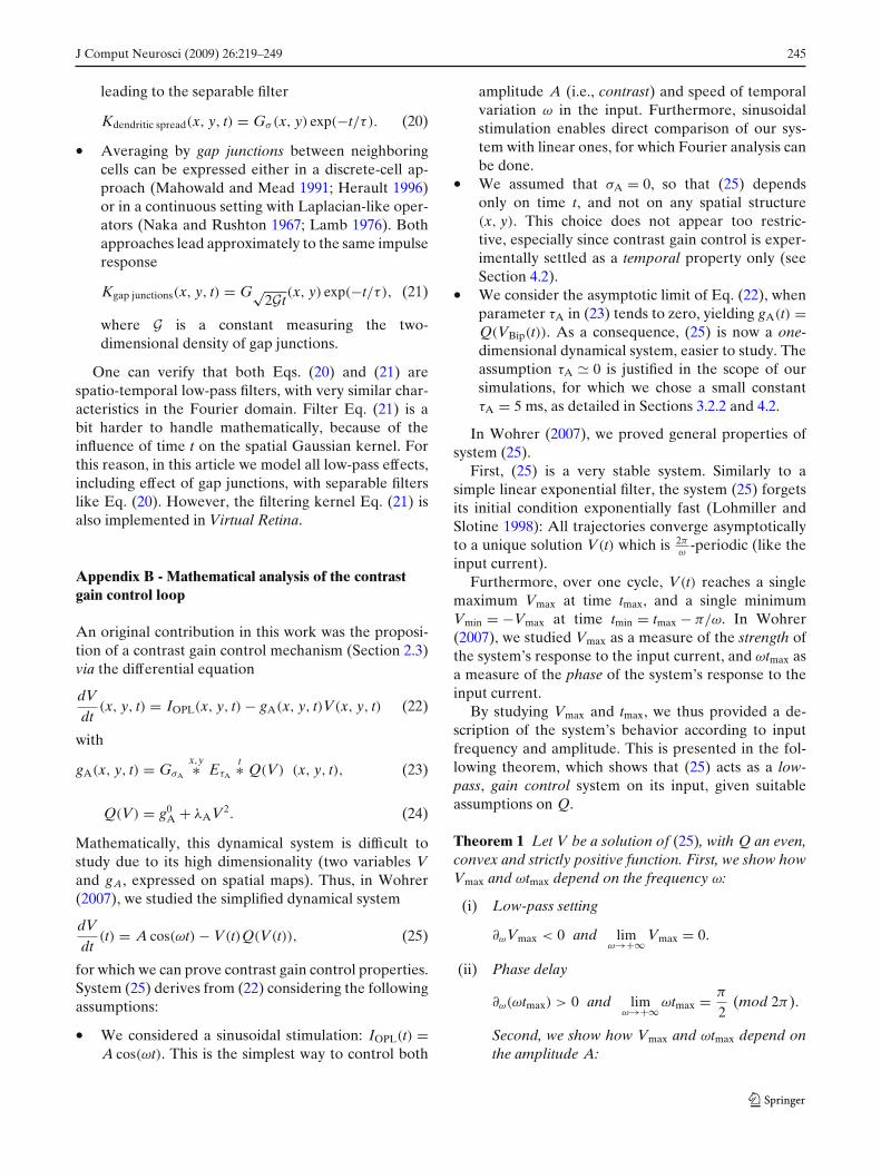
J Comput Neurosci (2009) 26:219–249 245
leading to the separable filter
Kdendritic spread(x, y, t) = Gσ (x, y) exp(−t/τ). (20)
• Averaging by gap junctions between neighboringcells can be expressed either in a discrete-cell ap-proach (Mahowald and Mead 1991; Herault 1996)or in a continuous setting with Laplacian-like oper-ators (Naka and Rushton 1967; Lamb 1976). Bothapproaches lead approximately to the same impulseresponse
Kgap junctions(x, y, t) = G√2Gt(x, y) exp(−t/τ), (21)
where G is a constant measuring the two-dimensional density of gap junctions.
One can verify that both Eqs. (20) and (21) arespatio-temporal low-pass filters, with very similar char-acteristics in the Fourier domain. Filter Eq. (21) is abit harder to handle mathematically, because of theinfluence of time t on the spatial Gaussian kernel. Forthis reason, in this article we model all low-pass effects,including effect of gap junctions, with separable filterslike Eq. (20). However, the filtering kernel Eq. (21) isalso implemented in Virtual Retina.
Appendix B - Mathematical analysis of the contrastgain control loop
An original contribution in this work was the proposi-tion of a contrast gain control mechanism (Section 2.3)via the differential equation
dVdt
(x, y, t) = IOPL(x, y, t) − gA(x, y, t)V(x, y, t) (22)
with
gA(x, y, t) = GσA
x,y∗ EτA
t∗ Q(V) (x, y, t), (23)
Q(V) = g0A + λAV2. (24)
Mathematically, this dynamical system is difficult tostudy due to its high dimensionality (two variables Vand gA, expressed on spatial maps). Thus, in Wohrer(2007), we studied the simplified dynamical system
dVdt
(t) = A cos(ωt) − V(t)Q(V(t)), (25)
for which we can prove contrast gain control properties.System (25) derives from (22) considering the followingassumptions:
• We considered a sinusoidal stimulation: IOPL(t) =A cos(ωt). This is the simplest way to control both
amplitude A (i.e., contrast) and speed of temporalvariation ω in the input. Furthermore, sinusoidalstimulation enables direct comparison of our sys-tem with linear ones, for which Fourier analysis canbe done.
• We assumed that σA = 0, so that (25) dependsonly on time t, and not on any spatial structure(x, y). This choice does not appear too restric-tive, especially since contrast gain control is exper-imentally settled as a temporal property only (seeSection 4.2).
• We consider the asymptotic limit of Eq. (22), whenparameter τA in (23) tends to zero, yielding gA(t) =Q(VBip(t)). As a consequence, (25) is now a one-dimensional dynamical system, easier to study. Theassumption τA � 0 is justified in the scope of oursimulations, for which we chose a small constantτA = 5 ms, as detailed in Sections 3.2.2 and 4.2.
In Wohrer (2007), we proved general properties ofsystem (25).
First, (25) is a very stable system. Similarly to asimple linear exponential filter, the system (25) forgetsits initial condition exponentially fast (Lohmiller andSlotine 1998): All trajectories converge asymptoticallyto a unique solution V(t) which is 2π
ω-periodic (like the
input current).Furthermore, over one cycle, V(t) reaches a single
maximum Vmax at time tmax, and a single minimumVmin = −Vmax at time tmin = tmax − π/ω. In Wohrer(2007), we studied Vmax as a measure of the strength ofthe system’s response to the input current, and ωtmax asa measure of the phase of the system’s response to theinput current.
By studying Vmax and tmax, we thus provided a de-scription of the system’s behavior according to inputfrequency and amplitude. This is presented in the fol-lowing theorem, which shows that (25) acts as a low-pass, gain control system on its input, given suitableassumptions on Q.
Theorem 1 Let V be a solution of (25), with Q an even,convex and strictly positive function. First, we show howVmax and ωtmax depend on the frequency ω:
(i) Low-pass setting
∂ωVmax < 0 and limω→+∞ Vmax = 0.
(ii) Phase delay
∂ω(ωtmax) > 0 and limω→+∞ ωtmax = π
2(mod 2π).
Second, we show how Vmax and ωtmax depend onthe amplitude A:

246 J Comput Neurosci (2009) 26:219–249
Fig. 12 Sample XML file used by Virtual Retina to load the architecture and parameters of the used model. This file is highly modular

J Comput Neurosci (2009) 26:219–249 247
(iii) Growth of Vmax
∂AVmax > 0 and limA→+∞
Vmax = +∞.
(iv) Phase advance
∂Atmax < 0 and limA→+∞
ωtmax = 0 (mod 2π).
(v) Under-linearity
∀ (ω, Q), if A is high enough, ∂AVmax
A < 0.
Also, limA→+∞
Vmax
A= 0.
Let us comment those results.Properties (i) and (ii) show that system (25) acts as a
low-pass temporal filter (using a classical linear systemsterminology). To understand this, suppose that Q(V) =g0
A, i.e., just a constant function. This means having anull feedback strength λA in Eq. (24). Then, Eq. (25)becomes a simple exponential low-pass filter
V̇(t) = A cos(ωt) − g0AV(t), (26)
whose behavior is well known:
Vmax = |H̃(ω)|A (27)
ωtmax = arg(H̃(ω)), (28)
where H̃(ω) = 1/(g0A + jω) is the Fourier transform of
the system. One verifies easily that Eqs. (27)–(28) implythat Vmax tends to 0 (with Vmax > 0) and ωtmax tends toπ2 (ωtmax < π
2 ), as ω → +∞. Properties (i)–(ii) extendthese properties in the nonlinear case of (25).
Properties (iii), (iv) and (v) show the apparition ofgain control in system (25), as opposed to the linearcase (26). In the linear case, Eqs. (27)–(28) give alinear dependence of Vmax and tmax with respect toamplitude A. One has indeed ∂AVmax = |H̃(ω)| > 0,∂A(Vmax/A) = 0 and ∂A(ωtmax) = 0. In the nonlinearcase (25), property (iii) shows that Vmax is still a growingfunction of A. However, this growth is now under-linear(property (v)).
Finally, property (iv) shows the phase advance effect,with input amplitude A. This second nonlinear effectcorresponds to the definition of contrast gain control inreal retinas, as detailed in Section 3.2.2.
Appendix C - Example of an XML configuration file
Figure 12 is a snapshot from an XML definition fileused in the simulator (with basis parameters for the X
cell modeled in Fig. 5(a)). Various XML nodes – suchas contrast gain control or the spiking array – can bepresent or absent from the file, adapting the simulatedmodel’s complexity in consequence.
In particular, a radial scheme can be present or not(here it is useless because a single cell is modeled).The spiking array can either be square, or made ofconcentric circles following retinal density (as here). Inthis example file, given the parameters of the circularspiking array, a single spiking cell is present (as usedfor reproduction of physiological recordings).
References
Baccus, S., & Meister, M. (2002). Fast and slow contrast adapta-tion in retinal circuitry. Neuron, 36(5), 909–919.
Bálya, D., Roska, B., Roska, T., & Werblin, F. S. (2002). ACNN framework for modeling parallel processing in a mam-malian retina. International Journal of Circuit Theory andApplications, 30(2–3), 363–393.
Barlow, H. B. (1953). Action potentials from the frog’s retina.Journal of Physiology, 119(1), 58–68.
Beaudoin, D. L., Borghuis, B. G., & Demb, J. B. (2007). Cel-lular basis for contrast gain control over the receptivefield center of mammalian retinal ganglion cells. Journal ofNeuroscience, 27, 2636–2645.
Bernadete, E. A., & Kaplan, E. (1999). Dynamics of primate Pretinal ganglion cells: Responses to chromatic and achro-matic stimuli. Journal of Physiology, 519(3), 775–790.
Bernadete, E. A., Kaplan, E., & Knight, B. W. (1992). Contrastgain control in the primate retina: P cells are not X-like,some M cells are. Visual Neuroscience, 8(5), 483–486.
Berry, M. J., Warland, D. K., & Meister, M. (1997). The struc-ture and precision of retinal spike trains. Proceedings of theNational Academy of Sciences of the United States ofAmerica, 94, 5411–5416.
Bonin, V., Mante, V., & Carandini, M. (2005). The suppressivefield of neurons in lateral geniculate nucleus. Journal ofNeuroscience, 25(47), 10844–10856, November.
Cai, D., Deangelis, G. C., & Freeman, D. (1997). Spatiotemporalreceptive field organization in the lateral geniculate nucleusof cats and kittens. Journal of Neurophysiology, 78(2), 1045–1061, August.
Carandini, M., Demb, J. B., Mante, V., Tollhurst, D. J., Dan, Y.,Olshausen, B. A., et al. (2005). Do we know what the earlyvisual system does? Journal of Neuroscience, 25(46), 10577–10597, November.
Chichilnisky, E. J. (2001). A simple white noise analysis of neu-ronal light responses. Network: Computation in Neural Sys-tems, 12, 199–213.
Chichilnisky, E. J., & Kalmar, R. S. (2002). Functional asymme-tries in ON and OFF ganglion cells of primate retina. Journalof Neuroscience, 22(7), 2737–2747, April.
Connaughton, V. P., & Maguire, G. (1998). Differential expres-sion of voltage-gated K+ and Ca2+ currents in bipolar cells inthe zebrafish retinal slice. European Journal of Neuroscience,10(4), 1350–1362, April.
Croner, L. J., & Kaplan, E. (1995). Receptive fields of P andM ganglion cells across the primate retina. Vision Research,35(1), 7–24, January.
248 J Comput Neurosci (2009) 26:219–249
Dacey, D., Packer, O. S., Diller, L., Brainard, D., Peterson, B.,& Lee, B. (2000). Center surround receptive field structureof cone bipolar cells in primate retina. Vision Research, 40,1801–1811.
Dacey, D., & Petersen, M. (1992). Dendritic field size and mor-phology of midget and parasol ganglion cells of the humanretina. Proceedings of the National Academy of Sciences, 89,9666–9670.
Delorme, A., Gautrais, J., VanRullen, R., & Thorpe, S. J. (1999).Spikenet: A simulator for modeling large networks of inte-grate and fire neurons. Neurocomputing, 26, 989–996.
Demb, J. B., Zaghloul, K., Haarsma, L., & Sterling, P. (2001).Bipolar cells contribute to nonlinear spatial summation inthe brisk-transient (Y) ganglion cell in mammalian retina.Journal of Neuroscience, 21(19), 7447–7454, October.
Dhingra, N. K., & Smith, R. G. (2004). Spike generator limitsefficiency of information transfer in a retinal ganglion cell.Journal of Neuroscience, 24, 2914–2922.
Enroth-Cugell, C., & Freeman, A. W. (1987). The receptive-fieldspatial structure of cat retinal Y cells. Journal of Physiology,384(1), 49–79.
Enroth-Cugell, C., & Robson, J. G. (1966). The contrast sensitiv-ity of retinal ganglion cells of the cat. Journal of Physiology,187, 517–552.
Enroth-Cugell, C., Robson, J. G., Schweitzer-Tong, D. E., &Watson, A. B. (1983). Spatio-temporal interactions in catretinal ganglion cells showing linear spatial summation.Journal of Physiology, 341, 279–307.
Erwin, H. (2004). http://scat-he-g4.sunderland.ac.uk/harryerw/phpwiki/index.php/tonicphasic.
Euler, T., & Masland, R. H. (2000). Light-evoked responses ofbipolar cells in a mammalian retina. Journal of Neurophysi-ology, 83(4), 1817–1829, April.
Flores-Herr, N., Protti, D. A., & Wässle, H. (2001). Synapticcurrents generating the inhibitory surround of ganglion cellsin the mammalian retina. Journal of Neuroscience, 21(13),4852–4863, July.
Gazeres, N., Borg-Graham, L., & Fregnac, Y. (1998). A phenom-enological model of visually evoked spike trains in cat genic-ulate nonlagged X-cells. Visual Neuroscience, 15, 1157–1174.
Gollisch, T., & Meister, M. (2008). Rapid neural coding in theretina with relative spike latencies. Science, 319, 1108–1111.doi:10.1126/science.1149639.
Gonzalez, R. C., & Woods, R. E. (1992). Digital image processing,3rd edn. Redwood City: Addison Wesley.
Hartveit, E., & Heggelund, P. (1994). Response variability ofsingle cells in the dorsal lateral geniculate nucleus of thecat. Comparison with retinal input and effect of brain stemstimulation. Journal of Neurophysiology, 72(3), 1278–1289.
Hennig, M. H., Funke, K., & Wörgötter, F. (2002). The in-fluence of different retinal subcircuits on the nonlinearityof ganglion cell behavior. Journal of Neuroscience, 22(19),8726–8738, October.
Herault, J. (1996). A model of colour processing in the retina ofvertebrates: From photoreceptors to colour opposition andcolour constancy phenomena. Neurocomputing, 12, 113–129.
Hérault, J., & Durette, B. (2007). Modeling visual perception forimage processing. In F. Sandoval, A. Prieto, J. Cabestany, M.Gra na, (Eds.), Computational and ambient intelligence : 9thinternational work-conference on artificial neural networks,IWANN 2007 (pp. 662–675). Springer.
Hochstein, S., & Shapley, R. M. (1976). Linear and nonlinearspatial subunits in Y cat retinal ganglion cells. Journal ofPhysiology, 262, 265–284.
Jacobs, A. L., & Werblin, F. S. (1998). Spatiotemporal patternsat the retinal output. Journal of Neurophysiology, 80(1),447–451, July.
Kaplan, E., & Bernadete, E. (2001). The dynamics of primateretinal ganglion cells. Progress in Brain Research, 134, 1–18.
Kara, P., Reinagel, P., & Reid, R. C. (2000). Low response vari-ability in simultaneously recorded retinal, thalamic, and cor-tical neurons. Neuron, 27(3), 635–646. Poisson, retina, spikevariability.
Keat, J., Reinagel, P., Reid, R. C., & Meister, M. (2001). Predict-ing every spike: A model for the responses of visual neurons.Neuron, 30, 803–817.
Kenyon, G. T., & Marshak, D. W. (1998). Gap junctions withamacrine cells provide a feedback pathway for ganglioncells within the retina. Proceedings of the Royal Society B,265(1399), 919–925, May.
Kenyon, G. T., Theiler, J., George, J. S., Travis, B. J., &Marshak, D. W. (2004). Correlated firing improves stimulusdiscrimination in a retinal model. Neural Computation, 16,2261–2291.
Kim, K. J., & Rieke, F. (2001). Temporal contrast adaptation inthe input and output signals of salamander retinal ganglioncells. Journal of Neuroscience, 21(1), 287–299, January.
Kim, K. J., & Rieke, F. (2003). Slow Na+ inactivation and vari-ance adaptation in salamander retinal ganglion cells. Journalof Neuroscience, 23(4), 1506–1516, February.
Kolb, H., Fernandez, E., & Nelson, R. (2001). Webvision:The organization of the retina and visual system.http://webvision.med.utah.edu/.
Kuffler, S. W. (1953). Discharge patterns and functional organi-zation of mammalian retina. Journal of Neurophysiology, 16,37–68.
Lamb, T. D. (1976). Spatial properties of horizontal cell re-sponses in the turtle retina. Journal of Physiology, 263(2),239–55.
Lesica, N. A., & Stanley, G. B. (2004). Encoding of natural scenemovies by tonic and burst spikes in the lateral geniculatenucleus. Journal of Neuroscience, 24(47), 10731–10740.
Lohmiller, W., & Slotine, J. J. (1998). On contraction analysis fornon-linear systems. Automatica, 34(6), 683–696, June.
McMahon, M. J., Lankheet, M. J. M., Lennie, P., & Williams,D. R. (2000). Fine structure of parvocellular receptive fieldsin the primate fovea revealed by laser interferometry. Jour-nal of Neuroscience, 20(5), 2043–2053, March.
McMahon, M. J., Packer, O. S., & Dacey, D. M. (2004). Theclassical receptive field surround of primate Parasol ganglioncells is mediated primarily by a non-GABAergic pathway.Journal of Neuroscience, 24(15), 3736–3745, April.
Mahowald, M. A., & Mead, C. (1991). The silicon retina.Scientific American, 264(5), 76–82.
Manookin, M., & Demb, J. (2006). Presynaptic mechanism forslow contrast adaptation in mammalian retinal ganglioncells. Neuron, 50(3), 453–464.
Mao, B. U. Q., Macleish, P. R., & Victor, J. D. (1998). Theintrinsic dynamics of retinal bipolar cells isolated from tigersalamander. Visual Neuroscience, 15(3), 425–438.
Marmarelis, P. Z., & Naka, K. (1972). White-noise analysis of aneuron chain, an application of the Wiener theory. Science,175(4027), 1276–1278, March.
Martinez-Conde, S., Macknik, S. L., & Hubel, D. H. (2004). Therole of fixational eye movements in visual perception. NatureReviews Neuroscience, 5, 229–240.
Masland, R. (2001). The fundamental plan of the retina. NatureNeuroscience, 4(9), 877–886, September.
J Comput Neurosci (2009) 26:219–249 249
Moisan, M. (2007). http://www.flickr.com/photos/marchelino/.Naka, K. I., & Rushton, W. A. (1967). The generation and spread
of s-potentials in fish (cyprinidae). Journal of Physiology,192(2), 437–61, September.
Nawy, S. (2000). Regulation of the On bipolar cell mGluR6 path-way by Ca2+. Journal of Neuroscience, 20(12), 4471.
Neuenschwander, S., & Singer, W. (1996). Long-range syn-chronization of oscillatory light responses in the cat retinaand lateral geniculate nucleus. Nature, 379(6567), 728–732,February.
Nirenberg, S., & Meister, M. (1997). The light response of retinalganglion cells is truncated by a displaced amacrine circuit.Neuron, 18, 637–650.
O’Brien, B. J., Isayama, T., Richardson, R., & Berson, D.M. (2002). Intrinsic physiological properties of cat retinalganglion cells. Journal of Physiology, 538(3), 787–802.
Polans, A., Baehr, W., & Palczewski, K. (1996). Turned on byCa2+! The physiology and pathology of Ca2+-binding pro-teins in the retina. Trends in Neurosciences, 19(12), 547–554,December.
Raviola, E., & Gilula, N. B. (1973). Gap junctions between pho-toreceptor cells in the vertebrate retina. Proceedings of theNational Academy of Sciences, 70(6), 1677–1681, June.
Rieke, F. (2001). Temporal contrast adaptation in salamanderbipolar cells. Journal of Neuroscience, 21(23), 9445–9454,December.
Roska, B., & Werblin, F. (2001). Vertical interactions across tenparallel, stacked representations in the mammalian retina.Nature, 410, 583–7, March.
Van Rullen, R., & Thorpe, S. (2001). Rate coding versus tempo-ral order coding: What the retina ganglion cells tell the visualcortex. Neural Computing, 13(6), 1255–1283.
Schnapf, J. L., Nunn, B. J., Meister, M., & Baylor, D. A. (1990).Visual transduction in cones of the monkey macaca fascicu-laris. Journal of Physiology, 427(1), 681–713.
Shapley, R. M., & Victor, J. D. (1978). The effect of contrast onthe transfer properties of cat retinal ganglion cells. Journalof Physiology, 285(1), 275–298.
Shiells, R. A., & Falk, G. (1999). A rise in intracellular Ca2+underlies light adaptation in dogfish retinal ‘on’ bipolar cells.Journal of Physiology, 514(2), 343–350.
Solomon, S. G., Peirce, J. W., Dhruv, N. T., & Lennie, P. (2004).Profound contrast adaptation early in the visual pathway.Neuron, 42, 155–162, April.
Tan, S., Dale, J., & Johnston, A. (2003). Performance of threerecursive algorithms for fast space-variant gaussian filtering.Real-Time Imaging, 9, 215–228.
Valeton, J. M., & Van Norren, D. (1983). Light adaptation of pri-mate cones : An analysis based on extracellular data. VisionResearch, 23(12), 1539–1547.
van Hateren, J. H., & Lamb, T. D. (2006). The photocurrentresponse of human cones is fast and monophasic. BMCNeuroscience, 7(1), 34–41.
van Hateren, J. H., Rüttiger, L., Sun, H., & Lee, B. B. (2002).Processing of natural temporal stimuli by macaque reti-nal ganglion cells. Journal of Neuroscience, 22(22), 9945–9960.
Victor, J. D. (1987). The dynamics of the cat retinal X cell centre.Journal of Physiology, 386(1), 219–246.
Werblin, F. S., & Dowling, J. E. (1969). Organization of theretina of the mudpuppy. Journal of Neurophysiology, 32(3),339–355.
Wohrer, A. (2007). Mathematical study of a neural gain controlmechanism. Research report 6327, INRIA.
Wohrer, A. (2008a). Model and large-scale simulator of a biolog-ical retina with contrast gain control. PhD thesis, Universityof Nice Sophia-Antipolis.
Wohrer, A. (2008b). The vertebrate retina: A functional review.Research Report 6532, INRIA, May.