VIRTUAL PLANKTON ECOLOGY - Virtual Ecologyvirtualecology.org/vpebook/chapter2_agents.pdf · Virtual Plankton Ecology - Chapter 2 VPE Book chapter 2.doc Last printed 12/11/2009 18:59

Virtual Plankton Ecology - Chapter 2

VPE Book chapter 2.doc Last printed 12/11/2009 18:59 Page 1 of 72

VIRTUAL

PLANKTON ECOLOGY

Usingtheprimitiveequationsofmarinephysics,chemistryandbiology

tosimulatetheplanktonecosysteminthesea

Chapter 2 Agent-based computation

John Woods & Silvana Vallerga

Imperial College London and

Consiglio Nazionale delle Ricerche (ISMAR) Genoa

Monograph

Chapter2VersionforcommentSeptember2009





2 Agent-based computing

1. Summary

2. IntroductiontoAgent‐basedcomputing

3. ABCinvirtualplanktonecology

4. Goals

5. Mesocosm

6. Virtualecosystem

7. Forcing

8. Environment

9. Particles

10. Ambientenvironment

11. Planktonassociatedwithaparticle

12. Modelplanktoncommunity

13. Toppredators

14. Sub‐populations

15. Biologicalprocesses

16. Species

17. Biologicalconditionofaplankter

18. Particlesspawningnewparticles

19. Demography

20. Biologicalenvironment

21. Biofeedback

22. Particleinteractions

23. Qualitycontrol

24. Planktonica

25. VirtualEcologyWorkbench

26. CreatingaVPE

27. DiagnosingaVPE

28. Practicallimitstocomputing

29. Conclusion





Summary

This chapter is about computation. It introduces agent-based computing (ABC) and

shows how the technique has been adapted to simulate plankton life histories. It

describes the allocation of a dynamic sub-population of identical plankters to each

agent. That makes it possible to take account of every plankter in a virtual ecosystem,

which is essential for budgeting ecosystem properties accurately.

But that is only half of the story. The other half is concerned with computing the fields

that describe the environment. Simulating the ecosystem requires careful computation

of the two-way interaction between these fields and the plankton agents. Equally

important is accurate computation of the two core properties of ecology: demography

and biofeedback. They involve summing over all agents present in each element of the

mesh used to define the fields.

The Lagrangian Ensemble (LE) metamodel combines all these ABC procedures in a

consistent framework for creating virtual plankton ecosystems. The computations are

presented in three parts. The first describes the virtual mesocosm with its mesh,

environmental fields and forcing by exogenous phenomena. The second part focuses

on the particles that are represented by computer agents; it describes their

trajectories and ambient environments. Each particle has a dynamic sub-population

of plankters with the same biological state and biochemical state, changes in which

are computed using phenotypic rules. The third part describes ecological phenomena,

especially demography, biofeedback and biological environment. This leads to a

discussion of how to model predation. It is computed for each particle interacting

with its biological environment. Particle management procedures control the quality

of emergent properties. Each VPE is described completely by its specification; two

computer runs with same specification produce identical VPEs. Planktonica uses just

nine function calls to program all these computations. It is embedded in the Virtual

Ecology Workbench (VEW), which automates the creation and diagnosis of virtual

ecosystems. The chapter describes how a VPE is created and analysed by following

the step-by-step instructions displayed on the VEW graphical user interface. The

Virtual Ecology Workbench provides a complete implementation of agent-based

modelling for plankton ecology.





2.1 IntroductiontoAgent‐basedcomputing

Agent-based computing simulates the history of discrete entities in a complex system

as they interact with their environment, responding to and modifying it. (Jennings

2000) discusses the pros and cons of this increasingly popular technique from the

viewpoint of a software engineer. (Luck, McBurney et al. 2005) provide a useful

“ABC roadmap” based on the European Commission Agentlink program. There is a

growing literature on ABC software engineering; see, for example the much-cited

publications by (Jennings 1999; Jennings 2000; Jennings 2001) and (Zambonelli,

Jennings et al. 2003). In brief, ABC is now mature and ready for modelling practical

systems.

In the past, agent-based modelling involved programming by scientists using Fortran.

That continues today, but it is labour intensive and produces ponderous code (Grimm

and Railsback 2005). The burden can be reduced by using programming languages

such as SWARM, which contains a library of functions designed to facilitate ABC

modelling of complex adaptive systems (Minar, Burkhart et al. 1996); see also

http://www.swarm.org. Ecosim and WESP provide more focused ABC frameworks

for ecological modelling (Lorek and Sonnenschein 1999). See also (Ginot, Le Page et

al. 2002). For Virtual Plankton Ecology we have (Hinsley 2005)’s Planktonica

language for ABC modelling, and his Virtual Ecology Workbench (Hinsley 2007)

(see §2.25 and chapter 7). The message is that investment in advanced software

engineering can eliminate many of the problems associated with conventional Fortran

programming.

Having indicated those computing foundations we now consider how ABC is applied

to modelling complex systems. (Billari, Fent et al. 2006) highlight its special

character: “Agent-based computational models pre-suppose rules of behaviour [for

each agent] and verify whether these micro-based rules can explain macroscopic

regularities”. In Part 3 of this book we shall re-examine the paradigms of biological

oceanography. Our aim is to show how ABC can produce a higher level of

understanding than could be achieved with traditional methods like population-based

modelling. Using ABC enriches our intuition about the ecosystem. (Axelrod 1997)

neatly captured this idea: “Whereas the purpose of induction is to find patterns in data

and that of deduction is to find consequences of assumptions, the purpose of agent-



based modelling is to aid intuition”. The simulated data of agent-based models can be

analysed inductively, even though the data are not from the real world.

2.1.1 ABCapplications

Starting in the 1980s, ABC has been used to simulate a wide range of complex

systems in epidemiology, economics and the social sciences (Billari, Fent et al. 2006).

It has also been used to model commercial operations. The agents used in business

models represent entities that are familiar to most people. They provide an accessible

entry to agent-based modelling. So it is worth spending some time considering an

ABC business model before embarking on the intricacies of the plankton ecosystem.

The Container World project1 led by John Woods at Imperial College London

illustrates the state of the art in ABC business modelling (Polak, Carter et al. 2004),

(Sinha-Ray, Carter et al. 2003) (Polak, Carter et al. 2003).

2.1.2 TheContainerWorldmodel

The CW project models the global transport of freight in containers; 80% of world

trade. It features coupled simulations of the logistics and finances of the container

business. That had never been attempted before. The goal was to provide a software

tool that could be used by government agencies and commercial enterprises to support

planning and investment decisions.

When CW was first proposed the globalization of world trade was in full swing, with

a 9% annual growth of container traffic per year. This posed serious challenges for

businesses making decisions on investment in new ports, depots, ships, trains, trucks

and containers. Container transport was a very dynamic global business, with

successful companies taking over rivals that failed to get their business model right.

The challenge has become much more severe in the present global recession, which

has seen a substantial decrease in world trade and freight charges, and problems in

raising money to invest in new assets.

The original motivation for the Container world project was to create the first-ever

comprehensive model of the world freight business. Previously each business and

government relied on empirical models of their own sector. Those models were based

on statistics collected annually and extrapolated into the future on the basis of

1 http://www3.imperial.ac.uk/earthscienceandengineering/research/energyenvmodmin/container%20world



business plans. The strategy for the Container World project was to use ABC, so that

data for the agents and equations for their operations would provide powerful

constraints on the emergent properties of the simulation, including such factors as

road, rail and port congestion, and the profits and losses of the competing businesses.

The idea was that each businesses or government agency could run the CW model

with its own assumptions about future changes in world trade, and about their own

business models and those of their competitors. This method is called What-if?

Prediction (WIP). It differs from traditional practice by using a comprehensive global

model with constraints on every component provided by real data and micro-scale

equations.

The agents in the Container World (CW) model represent every container in the

world; also every ship that carries those containers, and every port that handles

containers. In addition to that global network, CW describes the over-land transport

system in Great Britain, with agents for every truck and train, terminal and depot. The

model contains comprehensive data for each of these agents. It also has a world map

with the standard shipping routes and, on land, the road and rail networks. The total

data and number of agents is quite large, but manageable on a personal computer. A

demonstration and training version of CW, which has a reduced data and number of

agents, runs on a laptop.

The transport model comprises rules for the movement of each container in time steps

of one day at sea, or 15 minutes on land. The rules describe the operations of each

ship, loading and unloading containers in port, motoring along the appropriate sea-

lane at a speed directed by the owner (the model has data on every ship). They were

derived from the current practice of leading companies and government agencies

participating in the business and advising the project. On land the container

movements by road or rail works within the constraints of the respective networks and

the known performance of each truck and train. Geographical locations are defined by

postcode, which in UK may identify a single large building, or a small cluster of

houses in one street.

The businesses owning these transport assets are also represented by agents in the

model. The model knows which business owns each port, depot, ship, truck, train, and

container listed in CW. Individual companies manage these assets. They direct the

movements of their containers around the world in their ships, moving along specified



routes, between specified ports. If necessary they rent additional resources to meet

their commitments.

The CW model is driven by a prescribed stream of invitations to tender for the

transport of specific freight. Some of these jobs are one-off (like moving granny’s

furniture from Melbourne to London) others involve regular movements at fixed

intervals on six months renewable contacts (e.g. motor cars from Japan to Europe, or

goods purchased by Walmart in China for sale in New York). The complex job stream

is based on analysis of records of the manifests of containers passing through ports

around the world in recent years. It is adjusted for the known annual growth and

changes in the pattern of world trade. This job stream is compiled in confidence by

the user as a key step in designing a What-if? prediction. It takes account of known

seasonality in demand for transport service (the pre-Christmas trade is a major

fraction of the annual total for many goods).

Shippers publish new jobs each day for all transport businesses to consider. Those

with spare capacity on the required route tender for the job at a price that takes

account of the costs that will be involved, and making the profit margin they have

decided in the company business plan. On the closing day the shipper ranks the

tenders for a particular job in terms of offer price and perceived reliability of the

tendering transport companies. (The model keeps track of late deliveries and rates

each company accordingly.) When a transport company wins a contract it is

committed to collecting the goods at the designated location (defined by a postcode, if

in UK; or by a depot if in another country for which the model does not yet include

overland transport), then loading the goods into one or more of its containers, and

transporting the container to the designated destination by the specified target date. In

practice a transport company normally aggregates the containers used for many

contracts into the load for one ship. Some containers may be stored temporarily at the

departure port until there is spare capacity on one of the company’s ships. On

occasion this can lead to late delivery, with a consequent loss of rating for the

company.

This process of inviting bids for new jobs, tendering, assessment and awarding

contracts is handled automatically by CW as a virtual e-business. Once the contract is

awarded for a job the model automatically manages all stages of the transport process

over land and sea. It also debits the transport company for costs incurred at each stage



(port storage and handling, wages, fuel and other ship costs, rental of containers, etc.).

The finances of each business are computed from these costs and the income from

shippers. Company analysts can use the CW model to analyse the earning

performance of individual ships and routes. They use such information to revise their

business plan and price list each year. The biggest item in the business plan concerns

the decision to sell old assets and buy new ones. The assets are costly, a ship or a port

crane cost tens of millions of pounds, and have an earning life of decades. Investment

decisions are base on assumptions about the future pattern of world trade, and on the

expected business plans of competitors.

Furthermore, the model automatically generates a manifest for the ship listing the

goods carried in each container; this is needed for clearing Customs at each port. The

model generates a life history of every ship and container, and records of ships

passing through each port and the containers loaded and unloaded. Certain

government agencies find it interesting to analyse these manifests to see which ships

spent time in particular ports, and how long individual containers sat empty on the

dockside. For example, Customs use the pattern of information to train staff in

selecting containers to open; most shipments pass through ports unexamined.

To summarize, the Container World model automatically manages the business of

transporting goods around the world in containers; also the important task of

redistributing empty containers from ports of importing countries to those of

exporting countries (e.g. from Britain to China). It manages the loading and unloading

of ships, and when necessary the temporary storage of loaded or unloaded containers

in ports. It ensures that the shipping companies cannot bid for a job when they do not

have the capacity to carry it out in their own containers on their own ships. Or if their

business plan permits, the model manages sub-contracting the job to other companies,

and/or lease assets temporarily. The model also manages the finances of this massive

global freight business taking account of every action of every agent. It allocates costs

and income to each company, keeping track of their finances.

The companies revise their business plan for operations and investment and their price

list annually. Before doing so they use the model to assess the future prospects of the

company with these proposed plans. The assessments involve a series of What-if?

predictions for various assumptions about the future pattern of world trade and the

likely business plans of their main competitors. One of the early successes of CW was



to show that coastal shipping could compete profitably with trucks moving

transporting Scotch whiskey (the biggest UK export in containers) to the principal

ports, which are located in southern England. Shifting from road to coastal shipping

was shown to reduce congestion and pollution significantly. The advantage of using

an ABC model over previous methods is that it incorporates data and operating rules

for each agent. That micro-scale information provides powerful constraints that make

What-if? prediction more realistic than the traditional methods, especially in times of

major change in global trade.

2.1.3 ABCinEcology

Agent-based computation has a long history in ecological modelling, where it is

called individual-based modelling (DeAngelis and Gross 1992), (Chon, Lee et al.

2009). Using agents to describe the histories of individual organisms permits

simulation of intra-population variability, absence of biases population based

modelling (Lomnicki 1988; Lomnicki 1992). (Grimm and Railsback 2005) introduced

the name Agent-Based Ecology (ABE) for simulations that satisfy a number of

criteria, including full life cycle simulation of individuals and biofeedback to the

environment. All their criteria are satisfied in the special case of VPE.

2.1.4 ABCinFisheries

Individual-based modelling (IBM) is popular among fisheries scientists (Van Winkle

and Rose 1993), (Werner, Quinlan et al. 2001). (Vabø and Nøttestad 2003) use IBM

to simulate fish school behaviour. IBM is used to follow the annual migration of fish

stocks. (Heath and Gallego 2006) focus on the use early life stages of fish. In the early

growth stages the fish are planktonic, and can be modelled within the LE metamodel

described in this chapter. This allows LE modelling of fisheries recruitment (see

ch.26). Larger growth stages of fish present a problem because, unlike plankton, they

can learn new behaviour. We do not yet have reliable primitive equations for learning,

so VPE is not used to model fish stocks, except in their early, planktonic phase.

2.2 ABCinvirtualplanktonecology

Virtual Plankton Ecology use ABC to simulate the plankton ecosystem in the ocean

by computing the life history of every plankter in a mesocosm, and the history of the

environment, taking account of (two-way) interaction between environment and



plankton. VPE differs significantly from the other applications discussed above

because it uses the primitive equations of physics, chemistry and biology to derive

rules for the physiology and behaviour of each agent (Woods 2002). Primitive

equations are derived from reproducible experiments performed under controlled

equations. They provide solid scientific foundations for VPE. Such foundations do not

exist in the social sciences. This chapter shows how ABC has been adapted to

simulate the plankton ecosystem. The emphasis here is on computing with just

enough science to make the target clear in each case. The next four chapters will

discuss the science in more detail.

Ecology involves both organisms (plankton in our case) and the environment in which

they live, and which they modify by biofeedback. The life histories of plankton are

computed by means of agents. The environment is represented by fields, whose

histories are computed by the traditional methods of continuum dynamics. The fields

are defined by a mesh, which divides the volume into cells. Each field has one value

in each mesh cell. One of the challenges of VPE is to compute the interaction between

plankton agents and environmental fields. This is a prerequisite for computing the two

quintessential properties of ecology: demography and biofeedback. It is also crucial

for computing the consequences of predation: ingestion by the predator, and depletion

of prey.

ABC simulates the history of each agent. When it is applied to plankton ecology the

simulation contains the life history of every plankter in the ecosystem. That

information is not available in any other method of simulation. It offers unique

benefits for diagnosing the complex changes that occur in an ecosystem. Remember

that macro-changes in the environment are due in part to the action of plankton, which

are in turn controlled by biological primitive equations. So the life histories of

individual plankters provide a bridge to explain macro environmental changes in

terms of primitive equations.

The number of agents that can be handled depends on the available computer. A

modern laptop can create a VPE with about one million agents. If more are needed it

is necessary to upgrade to a parallel computer. Most of the VPEs presented in this

book use fewer than one million agents to simulate a VPE in a one thousand cubic

metre mesocosm. Many more than one million plankters live in that volume in the



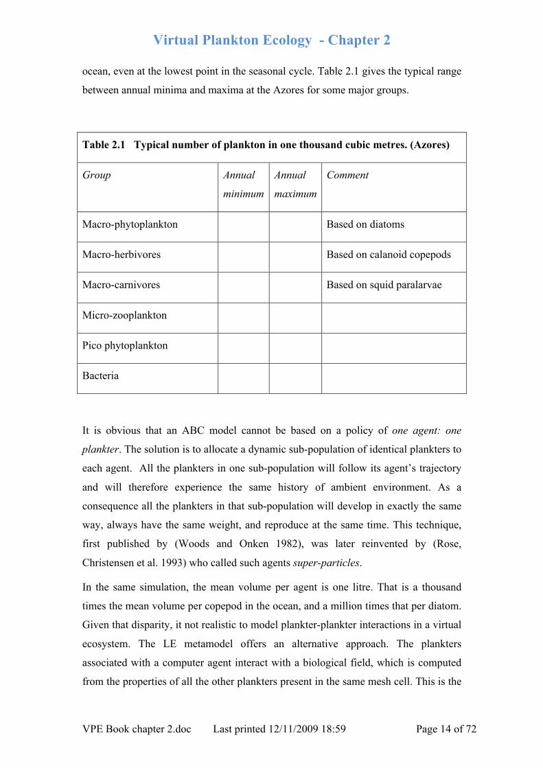
ocean, even at the lowest point in the seasonal cycle. Table 2.1 gives the typical range

between annual minima and maxima at the Azores for some major groups.

Table 2.1 Typical number of plankton in one thousand cubic metres. (Azores)

Group Annual

minimum

Annual

maximum

Comment

Macro-phytoplankton Based on diatoms

Macro-herbivores Based on calanoid copepods

Macro-carnivores Based on squid paralarvae

Micro-zooplankton

Pico phytoplankton

Bacteria

It is obvious that an ABC model cannot be based on a policy of one agent: one

plankter. The solution is to allocate a dynamic sub-population of identical plankters to

each agent. All the plankters in one sub-population will follow its agent’s trajectory

and will therefore experience the same history of ambient environment. As a

consequence all the plankters in that sub-population will develop in exactly the same

way, always have the same weight, and reproduce at the same time. This technique,

first published by (Woods and Onken 1982), was later reinvented by (Rose,

Christensen et al. 1993) who called such agents super-particles.

In the same simulation, the mean volume per agent is one litre. That is a thousand

times the mean volume per copepod in the ocean, and a million times that per diatom.

Given that disparity, it not realistic to model plankter-plankter interactions in a virtual

ecosystem. The LE metamodel offers an alternative approach. The plankters

associated with a computer agent interact with a biological field, which is computed

from the properties of all the other plankters present in the same mesh cell. This is the



origin of the name “Lagrangian Ensemble” used for this kind of ABC. In the name,

Lagrangian refers to the individual agent and Ensemble refers to all the other agents

in the same mesh cell.

This chapter will describe procedures to compute the biological field used in

simulating predation, both from the viewpoint of the individual predator (ingestion),

and from that of the ensemble of prey (depletion). Special care is needed to compute

the biological fields for zooplankton that migrate through several mesh cells in one

time step of the computation. The demography of each population is computed from

its biological field, i.e. from the ensemble of sub-populations in each mesh cell. The

demographic variables are (1) the number of plankters in the cell, (2) the rate of

increase by reproduction, (3) the rate of decrease by various causes of death

(starvation, senility, mortal disease, childbirth, or being eaten by a given species of

predator, including cannibalism by its own species), and (4) the life expectancy. Each

of these variables is expressed as a demographic field.

2.3 Goals

The goal of agent-based computation in plankton ecology is to generate mathematical

simulations – virtual ecosystems - that are rich in detail, and scientifically credible.

They support the activities discussed below.

2.3.1 Revealingandexplainingunexpectedphenomena

The first goal of virtual plankton ecology is exploration. Faced with a completely new

VPE, the challenge is to become familiar with the many aspects of the space-time

structure of its environmental fields, and to see how individual plankters respond to

the environment and how collectively they modify it. Months of careful analysis may

be needed to establish these facts about the virtual ecosystem. They will include

familiar phenomena, such as those described in Part 3. The challenge is to quantify

how those paradigms emerge in the particular circumstances of a VPE, with its

particular specification of model and forcing. However, detailed investigation may

also reveal unexpected phenomena. This is the quintessence of complexity science,

which deals with systems so rich in detail that they have scope to spring surprises. In

many cases it only takes a moment’s reflection to realize what is going on. But

sometimes the emergent phenomenon is not only unexpected, but counter-intuitive.



Intuition arises from previous experience and colours our expectations. It fits within

the linear world of classical induction. Many phenomena can only be explained by

non-linear actions; they need careful diagnosis with an open mind.

One of the joys of virtual plankton ecology lies in completeness. Every virtual

ecosystem contains not only a complex mass of interacting phenomena, but it also

contains all the information needed to explain those phenomena. The art of scientific

explanation is to show how macro phenomena arise inevitably from the actions of

micro processes. The macro phenomena of a VE are space-time patterns in the

environmental and demographic fields. The micro processes are those undertaken by

individual plankters, represented by computer agents. In VPE plankton processes are

controlled by phenotypic rules, which interpret primitive equations derived from

reproducible experiments. That allows us to explain macro patterns in the fields in

terms of the fundamental biological laws that control the plankton. This unique

property of virtual plankton ecosystems makes it possible to achieve Ernest

Rutherford’s prescription for science: “The art of science is to convert a mystery into

a commonplace.” The emergent space-time patterns in the fields of a VE may be

initially mysterious; but they can be explained without recourse to information outside

the VE. Once understood they can then be added to the list of paradigms, like those

featured in Part 3.

2.3.2 Teaching

Detailed analysis of a virtual ecosystem is directed towards understanding it. That

opens the way to using virtual ecosystems as tools for teaching plankton ecology. The

aim is to illustrate the subject’s paradigms. These are featured in textbooks and

underpin research. Part 3 of this book is devoted to showing how such paradigms

emerge in virtual ecosystems. The techniques described in this chapter allow us to

establish these paradigms on a sound scientific basis by exploiting the power of ABC

with primitive equations. The teacher can then use VPEs to illustrate selected

paradigms in his lecture course and in class work. In doing so he will note that the

illustration rests on a mathematical simulation that is provisional. It is likely to be

superseded by better VPEs based on revised specifications for the model and forcing.

The teacher will note the two methods used to upgrade the specification: testing

hypotheses and comparison with observations.



2.3.3 Investigatinghypotheses

A virtual ecosystem is the product of specifications for model and forcing. Each

contains uncertainties, some of which are known, others unknown. The VE must

always be treated as provisional, subject to future improvements in the specification.

Candidates for improvement must be treated as hypotheses. Investigating them is a

core research activity in virtual plankton ecology. One aim is to discover how

sensitive is the VE attractor to changes in the specification. For example, the model

plankton community contains only a selection of the species known to occur at the

chosen site. How does the attractor adjust when the selection is changed? When the

model community has been fixed, there remain uncertainties in the phenotypic

equations. The scientific literature may contain alternative versions. For example, the

choice of phenotypic rules for photosynthesis are quite different in the WB model

(Woods 2005) and the LERM model (Sinerchia, Vallerga et al. 2008). Finally, within

the chosen phenotypic rule, there may be uncertainty about the values of the

biological parameters. The sensitivity of the VE attractor to this uncertainty can be

established by scanning over the range of possible values.

2.3.4 Simulatingobservations

Comparing the VE with observations can guide one in designing a model plankton

community, and selecting phenotypic rules and parameters. The comparison is made

between an observed property and the corresponding emergent property of the VPE,

taking account of the uncertainties in each. The procedure, called the Ecological

Turing test, will be described in chapter 9. The goal is progressively to revise the VPE

specification until there is no statistically significant difference between observed and

emergent properties. The technique has been demonstrated by (Liu and Woods 2004;

Liu and Woods 2004).

2.3.5 Whatif?prediction

A VPE specification can be described as mature when it matches observations to the

limit of their information content, and when it bases the phenotypic rules on the best

available experimental data. Mature VPEs are always provisional, but provided they

have been thoroughly refined, they can be used operationally to make useful

predictions. This subject was discussed in chapter 1, where it was concluded that such

predictions can only be forecasts for a few days ahead, because the ecosystem is so

strongly influenced by the overlying weather, which cannot be forecast more than a



week ahead. So an operational prediction of the plankton ecosystem normally

comprises a hindcast perturbed by some artificial modification of the specification.

The aim is to see what happens when that change is made. Hence the name “What-if?

Prediction”.

2.3.6 Pre‐requisites

These applications provide tough specifications for virtual ecosystems. Each case is

different, but there are a number of issues that must always be considered in designing

a virtual ecosystem. Here we consider three issues: the signal-to-noise ratio, avoiding

constraints, and temporal resolution.

2.3.6.1 Signal‐to‐noiseratioThe emergent properties of the VE must have signal-to-noise ratios that allow one to

draw conclusions about cause and effect in the virtual ecosystem with a low level of

uncertainty. This applies to both the primary emergent properties (state variables of

the computation) and the secondary emergent properties (such demography and

biofeedback).

2.3.6.2 AvoidingconstraintsIt is equally important to avoid constraints that might prevent the virtual ecosystem

from adjusting freely to its attractor. That is achieved by careful specification of the

exogenous properties that force the virtual ecosystem. It is bad modelling practice to

prescribe the history of a state variable (such as the turbocline depth), which is a

primary emergent property of the VE. That may seem obvious. Nevertheless, the

scientific literature on modelling the plankton ecosystem contains many examples in

which prior constraints on mixed layer depth provoke unrealistic phenomena, even

chaotic fluctuations.

2.3.6.3 Temporalresolution

A third pre-requisite concerns the temporal resolution of the computation. The solar

diurnal cycle plays an important role in controlling the structure of the environment

(e.g. the diurnal thermocline) and in providing cues for plankton behaviour (e.g. diel

migration). So it is essential that the computation uses a time step that resolves these

diurnal phenomena adequately. Most of the numerical experiments in Part 3 of this

book use a time step of 30 minutes. 48 values per day are sufficient to describe

sinusoidal phenomena like the diurnal cycle of insolation. However, zooplankton



response is not sinusoidal; it is skewed with rapid descent around dawn to reduce

losses to visual predators. The risk of being seen and eaten depends on a complex

interaction between turbulence and migration (see chapter 10). A time step of less

than 30 minutes may be needed to resolve that interaction with acceptable accuracy.

(Barkmann and Woods 1996) found it necessary to use a 5-minute time step to resolve

the response of phytoplankton to turbulence (see chapter 31).

2.3.7 Conclusion

Virtual plankton ecology has many customers. In all cases it is necessary to pay

careful attention to quality control. We have highlighted three aspects: signal-to-noise

ratio, avoiding constraints, and resolving rapid change. Each application poses

different requirements that must be addressed in designing a virtual ecosystem. That

design translates into a specification for the computation. Of course this is true for all

mathematical simulation. But it requires special attention in agent-based computation

because of the complex interactions between the two components of the virtual

ecosystem: the fields describing environment, demography and biofeedback; and the

agents describing plankton as individual organisms.

2.4 Mesoscosm

A virtual plankton ecosystem is confined to an ocean mesocosm, which contains a

fixed volume of seawater. Most of the numerical experiments described in this book

are designed to simulate the average conditions in an area of one degree of latitude

and longitude, because that the spatial resolution of the exogenous forcing. These are

one-dimensional VEs with no horizontal structure. The exception is chapter 33, which

uses a 3D VPE to investigate plankton patchiness in the same 1°x1° zone.

2.4.1 Mesh

The distinction between one- and three-dimensional VEs rests on the mesh used to

define the environmental and demographic fields. In the one-dimensional VE the

mesh comprises a vertical stack of cells (often referred to as layers). They are one

metre thick in the one-dimensional VEs described in Part 3 of this book. Each layer

has a horizontal extent of one square metre. So the mesh cell has a volume of one

cubic metre. That leads to convenient units for budgeting (e.g. mgN/m3), but it is

merely a computational convention. Remember that the cell represents the mean



properties in its range of depths for a 1°x1° zone, which is roughly 100km x 100km.

The 1 cubic metre cell is simply a convenient sample of that much larger volume

(about 1012 cubic metres).

2.4.2 Units

It is important to remember this convention when discussing the number of plankton

in a one-metre-thick layer. The number of plankters in the layer is not an integer, but

the concentration per square metre on average in the 1°x1° zone. We shall see below

(§2.12) that this also applies to the number of plankters in the sub-population

associated with one computer agent. In §2.19 we shall see that the same units

convention applies to all demographic properties, whether associated with one agent,

one mesh cell, or the whole mesocosm. For example, the birth rate in one layer is

expressed as the number of new plankters created per cubic metre per second in that

depth range. This is the average value computed during one time-step of the virtual

ecosystem (typically half-an-hour, but sometimes shorter). It may seem more

convenient to quote demographic variables in units of per cubic metre per hour, but

the underlying biological equations are better expressed strictly in MKS units. (It is a

matter of choice for the modeller.)

2.4.3 Geographicallocation

The one-dimensional mesocosm has the form of a vertical cylinder, with its top at the

sea surface and its bottom at depth of typically one kilometre (although sometimes it

is only 500m deep). The mesocosm does not reach to the seabed; it ends in mid-water.

It is designed for use in the open ocean where the seabed lies at a depth greater than

one kilometre. This simplifies the bottom boundary condition. Perhaps in the future,

some brave soul will add seabed boundary conditions, so that the virtual ecosystems

can be designed to work on the continental shelf. Meanwhile, simulating the open

ocean ecosystem can make a substantial contribution to biological oceanography.

2.4.4 Adriftingmesoscosm

In its simplest form, the mesocosm is “moored” at a fixed location in the ocean. That

produces a geographically-eulerian virtual ecosystem (GEVE) as featured in (Woods

2005). However, much more can be learnt from a mesoscosm that drifts with the

ocean circulation. This is called a geographically-lagrangian virtual ecosystem



(GLVE). It provides valuable insight into how ocean currents influence on the

ecosystem (see ch.12).

Whether moored or drifting the mesocosm remains upright i.e. the axis of the cylinder

stays vertical. In a one-dimensional VPE, the mesh cells share the same geographical

footprint. In the moored case, the cells are not advected by the ocean currents. In the

drifting case they are all advected identically by the vertically averaged current (the

barotropic component of flow), but they are not advected by the baroclinic

component. Neglecting the shear in this way prevents the mesocosm from tipping

over. To summarize, a moored VE provides no information about the influence of the

circulation on the ecosystem. A drifting VE provides information about the response

of the ecosystem to the barotropic component of the flow, but none about the

baroclinic component. To fill that gap requires a mesoscosm with a three-dimensional

mesh (ch.30).

Water flows horizontally through the one-dimensional mesocosm, whether it is

moored or drifting. This relative horizontal flow is ignored in computing the

trajectories of plankters and other particles. Upwelling and turbulence can displace

particles vertically, but the geographical track of the mesocosm determines their

horizontal motion. Importantly, it is assumed that the horizontal flow through the

mesoscosm produces zero flux divergence in all environmental properties. Neglecting

the impact of horizontal flow through the one-dimensional mesocosm leads to error in

the virtual ecosystem. There is no internal evidence in the VE that might be used to

assess the magnitude of that error. However the error can be reduced by performing

numerical experiments at geographical locations where, according to published ocean

climatologies like NOAA’s (Levitus 1982), the flow is weak and horizontal gradients

are slack, so that the neglected flux divergences are likely to be small. The error can

be further reduced by choosing a geographical location (for a moored mesoscosm)

where (according to meteorological data like ERA40) the net annual heat flux through

the sea surface is zero. At such locations the total annual heating by the sun is

balanced by the heat loss from the ocean to the atmosphere, so the annual flux

divergence of heat due to ocean currents is also zero. This approach was used by

(Woods, Perilli et al. 2005) to study the long-term stability of a virtual ecosystem. We

shall have more to say in the next chapter about fluxes through the upper boundary of

the mesocosm. The lower boundary is open. Seawater can flow up or down through



it. This up- or down-welling is a component of the exogenous forcing used to create

the virtual ecosystem. Also particles are free to drop through the lower boundary into

the deep ocean below.

2.4.5 Laboratorymesocosms

The discussion so far has addressed large mesocosms in the open ocean. The methods

of virtual plankton ecology can also be used to simulate the ecosystem in a laboratory

mesocosm. In effect, the laboratory mesocosm is treated like an ocean mesocosm with

only one mesh cell. Marine biologists perform controlled experiments in laboratory

mesocosms to discover phenotypic rules for the biological functions of plankton

(REF). Agent-based modelling can prove useful for extracting phenotypic rules from

measurements made in these experiments (see Chapter 32).

2.5 Thevirtualecosystem

A virtual plankton ecosystem is a large data set, several gigabytes per simulated year,

which describes changes occurring in a model ecosystem located in the ocean

mesocosm. The virtual ecosystem comprises time series of emergent properties that

describe the environment and the plankton that live in it, also various kinds of

biogenic detritus. The virtual ecosystem may extend in time from one to many years;

there are examples in chapter 18 of changes occurring over one hundred years. The

changes are described by a time series of synoptic snapshots of the state of every

variable recorded at intervals of typically half-an-hour.

The virtual ecosystem is a solution to a mathematical problem, namely to describe

how a model ecosystem evolves when it is based on interaction between a specified

combination of endogenous processes and exogenous forcing. The problem is solved

by the Lagrangian Ensemble metamodel. The model obeys that metamodel: it

comprises rules used to upgrade the values of the model’s state variables each time

step. The recipe is written in the Specification for the virtual ecosystem. The

specification has three parts: the exogenous forcing, the endogenous model, and

technical procedures relating to the metamodel (§4.26). These will now be described

in outline.



2.6 Forcing

Five exogenous data sets are used to force the virtual ecosystem. They are ocean

circulation, nutrients, other initial conditions, boundary conditions, top predators and

events.

2.6.1 Oceancirculation

A dynamical model of ocean circulation is used to generate the velocity field needed

to compute advection of the mesocosm and upwelling inside it. The dynamical model

is not coupled to the VPE model: it is run separately. The velocity field is generated

and stored for use later as a resource when the virtual ecosystem is being created.

2.6.2 Nutrients

The biological production of the virtual ecosystem is limited by the nutrients specified

as initial conditions, or injected later in an event.

2.6.3 Otherinitialconditions

The values of all ecosystem state variables must be specified at the start of the

computation. These initial conditions come in two categories. The most important are

the nutrients, which limit biological production. The other state variables are less

important because over several years the virtual ecosystem will adjust to an attractor

that is independent of them (see chapter 11). That is true for both the plankton and the

environment apart from the nutrients.

2.6.4 Boundaryconditions

The surface boundary conditions are expressed as fluxes through the sea surface.

They are determined by exogenous properties, which by definition are unaffected by

the virtual ecosystem (see chapter 3). The challenge is to determine the values of the

fluxes at the current geographical location of the mesocosm, for the calendar year, day

of the year (taking account of leap years) and time of day2 when it is in the location.

The spatial variation is thereby assimilated into the time series of surface fluxes. Once

that time series has been computed there is no further need to take account of the

fixed/changing geographical location of the moored/drifting mesocosm. The time 2 VPE works in Greenwich Mean Time (GMT). The local time takes account of the mesocosm’s longitude. It is computed by adding one hour for every 15° longitude west of Greenwich. The Azores site used in numerical experiments in Part 3 is located at 27°N 40°W. So local noon at that site occurs at 14:40 GMT.



series of surface fluxes can be computed and stored before the computer run that

produces the virtual plankton ecosystem. Or they can be computed “on the fly” during

the computer run.

2.6.4.1 InsolationThe flux of solar radiation incident on the sea surface is expressed (by default in the

VEW) as a spectrum comprising 25 wavebands ranging from infrared to ultraviolet

with twelve bands in the photosynthetically active range (PAR, 400-700nm). The task

is to compute the surface downward irradiance in each of these wavebands. The

starting point is to use an astronomical equation to compute the solar elevation as a

function of latitude, day of the year and time of day. The next step is to compute the

change in irradiance as the solar beam passes through the atmosphere. This requires

the following atmospheric data: cloud cover (in different categories), dust

concentration, carbon dioxide concentration and humidity. The third step is to

compute the reflection of sunlight at the sea surface as a function of wave state. The

last step is to compute the refraction of the solar beam as it passes from air into water.

(Liu and Woods 2004) developed a practical model for computing insolation. It uses

the Monte Carlo method with one billion photons per waveband to synthesize the

spectrum of sunlight entering the ocean. The passage of each photon was computed as

is passes through the atmosphere and sea surface. The major factor is absorption and

scattering by clouds. There is also a probability that gases (including water vapour)

will absorb the photon and that Rayleigh scattering in the air and wave scattering at

the sea surface will deflect its trajectory. This high quality radiation model is

computationally expensive so it has not yet been incorporated into the virtual ecology

workbench. Meanwhile VEW4 uses a simpler empirical model based on (Paltridge

and Platt 1976).

2.6.4.2 Waterflux

The water balance of the uppermost layer of the mesocosm mesh has four elements.

The first two are universal: evaporation and precipitation, which increase and reduce

the layer’s salinity respectively. The third is run-off from the land, which applies in

coastal waters; this will become important in the future, when codes are available for

creating virtual ecosystems on the continental shelf. The fourth element is sea ice,

which has been modelled in polar and shallow high latitude seas such as the Baltic



(McPhee 2008). The present version of the virtual ecology workbench (VEW4) takes

account of only the first two elements (evaporation and precipitation).

The rate of evaporation (units: mm of H2O per second) is computed using the bulk

aerodynamic formula; see standard textbooks such as (Kraus and Bussinger 1994).

This formula involves a coefficient (parametrizing wave processes), the wind speed,

and the difference between the water vapour pressure in the lowest level of the

atmosphere and the saturated water vapour pressure of the sea (derived from the

temperature of the top layer of the mesocosm mesh).

2.6.4.3 HeatfluxThe heat balance in the uppermost layer of the mesocosm mesh has four elements.

The first three are universal: cooling by conduction to the air (sensible heat); cooling

by supply of latent heat to water vapour during evaporation; and cooling to supply

thermal (or long-wave) radiation emitted to the atmosphere, largely in the infrared

band (offset to some extent by heating due to absorption in the sea of thermal

radiation from the air.). The fourth element, which is not featured in VEW4, is

warming when seawater freezes at the base of a layer of sea ice, releasing latent heat

(McPhee 2008). The converse process, ice melting, occurs at the top of the layer of

sea ice, and the latent heat is taken up from the air.

The rate of cooling (units: Kelvin degrees per second, or K/s) by conduction is

computed by the bulk aerodynamic formula for sensible heat (Kraus and Bussinger

1994), which depends on a coefficient (parametrizing wave processes), the density

and specific heat of seawater, the wind speed, and the difference in temperature

between the lowest layer of the atmosphere and the uppermost layer of the mesocosm

mesh. The rate of cooling due to evaporation depends on the rate of evaporation, the

density and specific heat of water and the latent heat of evaporation. The rate of

cooling by thermal radiation is computed from the black body radiation formula,

which depends on the density and specific heat of seawater, and the temperature of

the uppermost layer of the mesocosm mesh) to the fourth power. The warming by

absorption of thermal radiation from the atmosphere uses the same black body

temperature, with the temperature and humidity of the lowest layer of the atmosphere.

It is assumed that all of the incoming thermal radiation is absorbed in the top one

metre of the ocean.



2.6.4.4 GasfluxesFluxes of oxygen, nitrogen, carbon dioxide and other gases through the sea surface

are computed using bulk gas transfer formulae (Kraus and Bussinger 1994), which

depend on a coefficient called the gas velocity because it has units of m/s, the wind

speed, and the difference between the partial pressures of the gas in the air and in the

top layer of the mesocosm mesh. The partial pressure of a gas dissolved in water

increases with water temperature. In the case of carbon dioxide the gas tends to flow

out of the ocean when it is warm (in summer) and into the ocean when it is cold (in

winter).

2.6.4.5 ParticulatefluxesThe flux of particles from the atmosphere can also be ecologically important.

Consider for example iron-rich dust from the Sahara, which enters the ocean in a

broad swathe extending across the Atlantic. The incoming particulate flux (units:

mol/m2s) enters the top layer of the mesocosm mesh, where it is treated as a

particulate concentration (mol/m3).

2.6.4.6 Momentumflux

The momentum flux from the atmosphere first enters the spectrum of wind-waves.

Breaking waves release momentum into the top layer of the mesocosm mesh. The

steady state momentum flux from the air is computed using the bulk aerodynamic

formula for momentum (Kraus and Bussinger 1994), which depends on a drag

coefficient (parametrizing waves processes), the density of air and the square of the

wind speed at a standard height (typically 10 metres) above sea level.

2.6.4.7 PowerintoturbulenceThe momentum entering the ocean also powers turbulence in the mixing layer. The

power entering the turbulence in the upper ocean sea (W/m2) can be equated to the

rate at which the wind does work against the friction presented by the sea surface. The

rate of work depends on the force times the speed of the object losing energy, in this

case the air. Equating the friction to the momentum flux in the bulk formula, this rate

of work depends on the cube of the wind speed. The turbulent kinetic energy is

transported downwards through the mixing layer. And the turbulence transports

momentum downwards to contribute to the wind-driven current. These dynamical

processes in the upper ocean will be discussed in chapter 4.



2.6.5 Toppredators

Top predators are members of the model plankton community. They prey on

zooplankton at a rate computed with a phenotypic rule, which is an endogenous part

of the model. However, the changing biological condition of the top predators, and

their demography and vertical distribution are all prescribed by exogenous rules and

parameter values, which are components of the forcing.

2.6.6 Events

Properties defined in the initial conditions can also be introduced later during the

computer run that creates a VPE. These events are also part of the forcing. They too

depend on exogenous data. Events can be used to describe phenomena as the injection

of chemical contaminants, or alien species in ship’s ballast water. They are a common

feature of numerical experiments in virtual plankton ecology.

2.7 Theenvironment

2.7.1 Fields

Each environmental property is represented in the mesocosm by a field, defined by

values in the mesh cells. The physical environment includes: solar irradiance (in 25

wavebands); temperature; salinity; seawater density (computed from temperature and

salinity); and turbulent kinetic energy. The last of these occurs in a “mixing” layer

extending down from the sea surface to the turbocline, below which the flow is

laminar for all practical purposes. The depth of the turbocline is resolved to one

millimetre; it is not constrained by the mesh resolution.

The chemical environment includes concentrations of the following classes of

chemicals: dissolved gases (notably oxygen, nitrogen, carbon dioxide); biogenic

dissolved inorganic chemical (DIN, DIC, etc.); and nutrients (phosphate, silicate,

nitrate, ammonium, etc).

2.7.2 Processes

The physical and chemical environment change in response to three phenomena: (1)

forcing by surface fluxes (see ch.3); physical transport processes inside the mesocosm

(see ch.4); and (3) consumption and biofeedback from the plankton (ch.6). Two sub-

models are used to compute the effect of physical processes on environmental

variables. The first computes the vertical profile of solar irradiance by one or other of



three methods: Empirical (Morel 1988), Monte Carlo (Liu and Woods 2004), or

Radiative Transfer Equation (Liu, Woods et al. 1999). The second, commonly known

as a mixed layer model, computes the depth of the turbocline and the profiles of

temperature, salinity and therefore density. Turbulence in the mixing layer

homogenizes the concentration of dissolved chemicals in the mixing layer. The

default mixed layer model used in VEW4 is due to (Woods and Barkmann 1986), but

it can easily be replaced by another. The current implementation of virtual plankton

ecology (in VEW4) does not feature chemical reactions in solution. The Revelle

equation is used to diagnose the saturated partial pressure of carbon dioxide in terms

of temperature and the concentration dissolved organic carbon. This is needed to

compute the air-sea flux of carbon dioxide (Revelle and Suess 1957).

2.8 Particles

2.8.1 Computeragents

A typical virtual plankton ecosystem, such as those described in Part 3 of this book,

contains order one million active computer agents. Agent life expectancy is shorter

than VPE duration. So a VPE will use many more agents than those active at any

time. They are used to describe the histories of living plankters and their detritus,

including fæcal pellets and the corpses of dead plankters. We often refer to agents as

particles; they are identical; one agent is one particle.

2.8.2 Namingparticles

Each particle has a name that can be used to identify it in a VPE. The naming

convention is designed to simplify analysis. One task is to identify the members of a

lineage, including all descendents of an initialization particle, or one injected later

during an event. (All particles spawned by one initialization or event particle are said

to belong to the same clan.) This is needed for scientific investigations of the spread

of inherited mutations (ch.18) or diseases (ch.22). It is also needed for quality control,

to ensure that computed demography is not biased by large sub-populations of

plankton on a few particles (Broekhuizen 1999). These tasks are complicated by

particle splitting and combination, which is featured in particle management, an LE

procedure that involves one particle spawning another, or two particles combining

(see §2.23). This procedure is used in quality control; it does not affect the biology or

demography of the plankton in the ecosystem.



A well-designed naming convention makes it simpler to devise analytical procedures

that deal automatically with these complications, allowing the modeller to concentrate

on the scientific problem. A practical naming convention must also avoid introducing

an undue computational burden when the virtual ecosystem is being created. There

can be tension between the software engineer designing an efficient program, and the

scientist wanting transparency in analysis. The solution is often a compromise

between these two goals. The VEW incorporates a naming convention that provides a

reasonable balance between computational efficiency and analytical convenience (see

chapter 7).

2.8.3 Particletrajectories

Agent-based computing is used to determine the trajectory of each named particle as

it moves up and down in the mesoscosm. Each particle follows an independent

trajectory. It is described by a three-dimensional Cartesian vector, x = longitude east

of Greenwich, y = latitude north of the equator, z = elevation above sea level (so

depth in the sea is negative). The particle’s depth is computed to an accuracy of better

than one millimetre in each direction. That resolution is not constrained by the size of

the mesh cells. The mesh is used to define environmental fields, not the trajectories of

particles.

In a one-dimensional virtual ecosystem, the particle’s latitude and longitude are

determined solely by the location of the mesocosm. The track of a drifting mesocosm

is computed by integrating the four-dimensional velocity field used to define the

ocean circulation. This integration normally involves a five-stage iterative procedure.

In three-dimensional virtual ecosystems the particle also moves horizontally within

the mesocosm. That motion is computed by integrating the mesoscale velocity field

inside the mesocosm. A three-dimensional vector in each mesh cell defines that

velocity field (see Chapter 30).

The vertical motion of a particle is computed by summing the displacements effected

by three processes: advection, turbulence and behaviour. The first is advection by

upwelling (or downwelling). The upwelling field is exogenous: it is a prescribed

feature of the external forcing; it is unaffected by the ecosystem. A particle’s ambient

upwelling is defined as the value of the upwelling field at its precise location. It is

computed either by using the field value in the mesh cell where the particle resides or



by curve fitting through nearby cells. The vertical particle displacement by advection

is computed by integrating this upwelling field defined by vectors in each mesh cell.

The second process is turbulence, which occurs only in the mixing layer, between the

sea surface and the turbocline (Ch.4). A particle’s turbulent displacement in one time

step is treated as a random process. It is computed with a random number generator

(RNG), which has a very long return time to avoid the risk of non-random repeats

during the period of the virtual ecosystem. The VEW uses the [REF] RNG algorithm,

which offers a sequence of xxx pseudo random numbers before repeating. That is

ample for a virtual ecosystem with one million particles lasting one million time steps

(roughly fifty years). The randomness of turbulent displacement causes the

trajectories of two initially close particles to diverge rapidly. Particles above the

turbocline are rapidly mixed (hence the name mixing layer). This leads to some

interesting ecological phenomena, like the Woods-Onken effect (see chapter 14).

Advection and turbulence move the particle with the water. The third process,

behaviour, moves the particle through the water. It arises in two ways: sinking or

swimming. The direction and magnitude of this vector depends on the biological

attributes of the particle, which may be a living plankter obeying phenotypic rules, or

detritus. All detritus particles and some plankton species sink (or float up) at a rate

prescribed in the model equations. Other species swim up or down (but not

horizontally) at a variable rate determined by their phenotypic rules. These equations

for plankton behaviour will be discussed in chapter 6. However it is worth making the

point here that some zooplankton are quite strong swimmers. Their behaviour is the

largest factor determining the particle’s change of depth in one time step when they

are in the non-turbulent thermocline. For example, adult copepods can swim several

metres per hour during their diel migration. This means they pass through several

mesh cells in one time step. To put it another way, while migrating they spend only a

fraction of one half-hour time step in each mesh cell. We shall see later that this

requires careful attention when we compute the fields of demography (§2.19) and

biological environment (§2.21).

That trajectory lies at the heart of virtual plankton ecology. The diversity of

trajectories is responsible for generating intra-population variability. It largely

determines the VPE’s computational complexity. The number of independent

trajectories (one per particle) determines the accuracy of all variables in the



ecosystem, the more the better. Considerable effort is needed to ensure that there are

always sufficient particles in every mesh cell. In virtual plankton ecology this is

achieved by the procedure called particle management (§2.23).

2.8.4 Orderofcomputation

During each time step, ABC upgrades the state of each particle (including in our case

its associated plankton and/or chemicals). It does so in an orderly way that keeps track

of each particle, so that individual histories can be revealed when we analyse the

virtual ecosystem. The order in which the particles are upgraded does not matter in a

simple ABC system, where the progress of one particle has no influence the others.

But that is not the case in virtual plankton ecology. The upgrading of one particle does

in this case affect the others. The influence is not direct. It is mediated through the

environment. Consider a particle that carries phytoplankton. Their biological

development depends on the uptake of nutrients and light, which are represented by

fields in the virtual ecosystem. As we shall see in chapter 6, these fields are

themselves affected by the actions of the plankton.

To give a simple example, each phytoplankton particle extracts nutrients causing the

field to become depleted partially or completely in the extreme case. The

phytoplankton associated with the first particle will experience the concentration of

nutrients left at the end of the last time step. But as the computation upgrades each

particle, its phytoplankton will experience a progressively depleted concentration of

nutrients, and will therefore grow less rapidly. The last in line, one million particles

later, may find the resource significantly depleted, even empty. So the order of

computation does matter in agent-based modelling. Or rather, it would if nothing were

done to ensure that the resources are equally available to all agents. In chapter 6 we

shall find out how the computation is modified to ensure that there is no

discrimination between the particles. While ABC does upgrade each particle in turn,

the practical computation uses a two-stage procedure to avoid bias.

The solution of this problem is equally important when computing the foraging

behaviour of zooplankton. Phenotypic equations in the model make the zooplankter

adapt to its recent history of ambient concentration of prey, which are of course

depleted during time step, so that early particles experience a difference prey

environment than those computed later. If uncorrected, that would lead to a bias in the



trajectories of zooplankton particles. As in the case of nutrient depletion, it is

necessary to introduce a procedure that ensures each particle experiences the same

prey concentration, taking account of the total depletion during the time step. This is

achieved by a two-stage process (§2.20).

2.8.5 Reproducibility

Consider two virtual ecosystems created by two independent runs on the same

computer. Suppose the specification is identical in the two runs, so that they have the

same model equations, forcing and initialization. The naming convention will allocate

the same set of names to the particles in the two virtual ecosystems. For every particle

in one VE there will be a doppelganger in the other, with the same name. Remember

that the specification for initialization includes the seed value for the random number

generator used to compute particle random displacement by turbulence. Provided the

two runs used the same seed value, doppelgangers in the two virtual ecosystems

follow the same trajectories and they experience the same histories of ambient

environment, so their plankton sub-populations have the same demographic and

biological histories and produce the same contribution to biofeedback.

On the other hand, if the two runs have identical specifications apart from the seed

value of the random number generator, doppelgangers will follow different

trajectories, and the environments in the two VEs will be different. Each will be a

valid solution of the model equations and exogenous forcing. Neither is more correct

than the other. We shall see in Chapter 11 how the virtual ecosystem can be

characterized by the statistics of an ensemble of instances, each differing only in the

seed value for the random number generator.

This ability to generate identical VEs in different runs with the same seed values

offers great practical benefits for the practice of virtual plankton ecology. For

example, it allows you to pursue an investigation of a VE piecemeal, logging in each

run only those emergent properties needed for that stage of an investigation. That

avoids the need to search through massive data sets, which would be the case if all

emergent properties were logged in the first run.

2.8.6 Chaos

It is well-known that even quite simple mechanical systems (for example a double

pendulum) do not follow the same history in successive runs (Longo 2009). That is



because the initial conditions are never exactly the same. Even the tiniest difference in

the launch conditions leads eventually to different histories of motion. This is an

example of the phenomenon of mathematical chaos described first by Poincaré in the

19th century (Poincaré 2001) and rediscovered periodically during the 20th century

(May 1976). However by imposing identical initial conditions, computer simulations

of such systems produce identical histories in two independent runs. We exploit that

property in performing numerical experiments with virtual plankton ecosystems (see

chapter 8). In chapter 11 we shall discover that the history of a virtual ecosystem has a

special nature. It adjusts to a stable attractor that is independent of biological initial

conditions (Woods, Perilli et al. 2005). That differs fundamentally from a simulation

of the same ecosystem created by a model with demographic state variables. In that

case the simulated ecosystem follows a more complicated and less predictable strange

attractor (May 1973).

2.9 Ambientenvironment

A plankter’s biological functions are expressed through phenotypic rules, which

describe how it responds to the environment in its immediate vicinity, which we call

the plankter’s ambient environment. Remember that the location of the agent carrying

the plankter in its sub-population is computed to an accuracy finer than one

millimetre. The agent lies in one of the mesh cells used to define the environmental

fields in the mesocosm. Each environment field is defined by values in the mesh cells.

The simplest way to compute the plankter’s ambient environment is to give it the

value for the mesh cell it occupies. A more sophisticated approach is to interpolate the

value by curve fitting through the data in nearby cells.3

2.10 Planktonassociatedwithaparticle

So far we have concentrated on the trajectories of particles (computer agents), without

specifying what they represent in the ecosystem. We have however noted that the

trajectories depend on the biological properties of the particles, which control their

swimming or sinking behaviour. Now we consider how particles are related to the

3 This is for a one-dimensional virtual ecosystem. Three-dimensional interpolation will be used for the VPEs described in chapter 32.



plankton and detritus in the ecosystem. As usual in this chapter, the focus will be on

computing principles, rather than on biology; that will come in chapter 6.

The application of agent-based computing to ecosystems is described well in the

textbook by (Grimm and Railsback 2005). It starts by allocating a computer agent to

each organism. The biological functions of the organism are described by phenotypic4

rules. We prefer to talk about rules rather than equations. This better matches the

reality of numerical computation, which updates the location of each agent and the

biological state of its plankter each time step. The phenotypic rule can be expressed in

narrative form as follows:

I am a plankter that is in the biological condition established during the previous time

step. The environment at my location (i.e. my ambient environment) can be found by

interpolation of the fields of environmental variables, which were also established

during the previous time step. My ambient environment includes physical, chemical

and biological variables. The last comprise the concentrations of predators and prey

and their biological and biochemical states. My phenotypic rules use that information

about my own state and my ambient environment to compute what my state will be at

the end of the current time step (after allowing for resource depletion by all the

plankton). Each rule updates some aspect of my biological state or determines my

behaviour, which will contribute to my change of location. It is a Boolean statement

of the kind:

“If this aspect of my state is X and the relevant ambient environmental variable has

the value Y, then the former will change by ±∂X (or I will sink/swim this far up/down)

during the current time step. Some of the rules govern metamorphosis: “If I am in

growth stage N and my lipid mass exceeds L, then I shall metamorphose into stage

N+1 and perform the various actions prescribed for that change, such as respiration

and moulting. 4 Phenotypic rules describe the biological function of the organism as a whole. Ecological applications tend not to get involved in the inner processes of organisms. At least not explicitly. For example they do not normally use equations for processes inside the cells of multi-cell organisms. However, LERM described in Ch.6 does include simple representation of internal organs, such as the gut. They also budget chemicals inside the organism, and rules for building proteins, lipids. LE models can include rules for making decisions; for example in migration and foraging behaviour, but they do not include any representation of the nervous system. These biological rules are crude parametrizations of cellular processes. The Virtual Ecology Workbench permits cellular processes to be included in LE modelling of the ecosystem.



Ideally such phenotypic rules are based on primitive equations derived from

reproducible experiments performed under controlled conditions. That is our goal in

virtual plankton ecology. It is more feasible with micro-organisms of limited motility

than for large animals and trees. Their biological functions tend to be described in

ABC models by more speculative rules, but not as insecure as those in social science

applications of ABC (Billari, Fent et al. 2006).

In virtual plankton ecology the phenotypic rules describe two kinds of biological

function: behaviour and physiology. We saw above that the trajectory of an agent that

represents a plankter depends in part on the plankter’s behaviour. We also noted that

the rules for behaviour might involve adaptation. For example, adaptation in foraging

behaviour can use a hunting rule: If I have passed through a maximum in the

concentration of prey, then I should reverse direction. The adaptation rule is hard

coded into the model. It cannot change during the computer run that produces a

virtual ecosystem. That is true for all the phenotypic rules. No part of the biological

model can change during a run. However, some of those rules describe how an agent

may adapt under prescribed conditions. In the terminology of complexity science the

virtual plankton ecosystem is non-adaptive. Most complexity scientists are devoted to

exploring adaptive systems, in which the rules do change during the run. We suspect

that the natural plankton ecosystem in the ocean is non-adaptive. Assuming that is

true, non-adaptive VPEs can address the core problem of biological oceanography,

which is to understand the observed space-time distributions of plankton in the sea.

VPEs are like simulations of the atmosphere by weather forecasters, which are also

non-adaptive. However, climate simulation is adaptive it includes economics and

politics.

2.11 Themodelplanktoncommunity

We have seen that the number of species in the ocean, even in the limited volume of a

mesocosm, greatly exceeds that in any realistic model. We can simulate only a small

fraction of the natural diversity. Given that technical problem it is useful to consider

some general guidelines for designing a model plankton community. The aim is to

create a VPE in which the ecological phenomenon being studied can emerge freely.

The first step is to identify the most prolific species encountered at the site and to rank

by their importance for the phenomenon being studied. This ranking refers to the



world of virtual ecology and not the natural ecosystem. It can be established by a

preliminary investigation (see chapter 18). The model community will normally

contain one or more of the highest ranked species in each trophic level, taking care to

include also those that provide the prey for featured zooplankton. The lower ranked

species can be grouped into functional groups (see chapter 6).

2.11.1 ToppredatorsTop predators feature in the model plankton community. They have conventional

phenotypic rules for ingestion, specifying the rate at which they eat their prey. A

community can include more than one top predator species, each feeding on different

prey species. The distinguishing feature of a top predator is that it’s biological

condition and its number concentration in each mesh cell are prescribed by exogenous

rules. Those properties change with time, but they do not depend on feeding success.

A top predator has no phenotypic rule for behaviour.

The rate at which these top predators deplete their prey provides the trophic closure

for the plankton model. We shall see in chapter 21 that the balanced state of a virtual

ecosystem, its attractor, is sensitive to the top predators. A small change in their

specification produces a trophic cascade that disturbs the demography of all species in

the model plankton community, and (because of biofeedback) all the environmental

fields. In chapter 11 we learn that the virtual ecosystem can take several years to

adjust to a new attractor when subjected to a disturbance by exogenous forcing. A

mesocosm can drift through geographical zones where different top predators are

active. To deal with this possibility, the model can include a set of top predators with

demographies whose exogenous rules for demography depend on the geographical

location of the mesocosm.

2.12 Sub‐populations

There is a technical innovation at the heart of virtual plankton ecology, which sets it

apart from the mainstream of ecological ABC described by (Grimm and Railsback

2005). The procedure allocates a dynamic sub-population of identical plankters to

each computer agent. This Lagrangian Ensemble method was introduced by (Woods

and Onken 1982). (Scheffer, Baveco et al. 1995) gave the name super-particles to

computer agents bearing sub-populations.



2.12.1 Computingdemographyandbiofeedback

The use of sub-populations is not optional in virtual plankton ecology. It is an

essential solution to the problem of using ABC to describe the plankton community in

the thousand cubic metres of an ocean mesocosm. As we have seen, in the ocean this

volume contains many billions of plankters. Computer limits normally constrain us to

use fewer than one million computer agents. Sub-populations makes it possible to

include all the plankters living in the virtual mesocosm. That opens the door to

computing the two quintessential properties of a dynamic ecosystem: demography and

biofeedback. These computations poll all the plankters living in the virtual ecosystem

contained in the ocean mesocosm. So it is an absolute pre-requisite for computing

demography and biofeedback that all the plankters of the model community be

represented in the virtual ecosystem. Using sub-populations makes that possible.

Every plankter in the virtual ecosystem can be found in the sub-population of one of

the particles.

2.12.2 Trajectoryunder‐sampling

In practice the modeller decides how many agents to allocate to each species (or

functional group) in the model plankton community. The number of plankters in

species/groups is invariably much greater than the number of agents.

All the plankters in one agent’s sub-population follow the same trajectory. We saw

earlier (§2.3) that the number of independent trajectories determine the degrees of

freedom in the population. So, although every plankter is accounted for in computing

demography and biofeedback, the plankters do not all have independent trajectories.

If they did, the computations of demography and biofeedback would be exact. But the

number of independent trajectories in a virtual ecosystem equals the much smaller

number of agents allocated to a species/group. So the computations of demography

and biofeedback suffer from uncertainties due to trajectory under-sampling.

2.12.3 ErrorsIf every agent allocated to a species/group had the same number of agents in its

subpopulations, and if its trajectory were random, then the error would be

proportional to the square root of the number of agents (trajectories) allocated to the

species/group. Using four times as many agents to the species/group would halve the

error. However, the sub-populations are dynamic. The number of plankters in the sub-



population of each agent changes according to the history of ambient environment

experienced along their trajectory. At any time step we can plot a histogram of the

number of agents with sub-populations in each of say a dozen ranges. If the histogram

has a Gaussian form, we can estimate the uncertainties in our calculations of

demography and biofeedback. The errors will be smaller if the range of sub-

populations sizes is smaller. The estimate of error is different if the distribution has a

non-Gaussian kurtosis. It will be biased if the distribution is skewed in favour of the

fatter sub-populations. In this case, the calculations of demography/biofeedback are

like those for a smaller number of agents/trajectories.

2.12.4 Managingerrors

It is important to limit the errors in demography and biofeedback, because they have

an impact on every emergent property of a virtual ecosystem. The errors reduce the

accuracy of predictions derived from the virtual ecosystem. We shall see in §2.23 that

practical virtual ecology includes a procedure to managing the distribution of sub-

populations in each species/group, and thereby limiting the errors in computing its

demography and biofeedback.

2.12.5 Sub‐populationbiologySo far we have focused on the reason why we use sub-populations, and the

consequences of that decision. Now we consider the relationship between sub-

populations and the biology of their plankters. Firstly, every plankter in a sub-

population is biologically identical. They all have the same biological state and

biochemical state. In any time step they all ingest the same number of prey and put on

weight, respire, excrete surplus chemicals and defæcate in the same way. They all

metamorphose from one biological state to the next in the same time step. Such

transitions include natural mortality, i.e. from living to dead. When ready to reproduce

they each produce the same number of offspring of the same birth weight. If infected

by a bacterial or viral disease, they all respond in exactly the same way.

2.12.6 Sub‐populationdepletionThe number of plankters in a sub-population are reduced by predation and natural

mortality (starvation, mortal disease, childbirth, old age, etc.). Consider the following

metaphor. The agent is like a sheep-pen. It contains a flock of sheep (herbivores),

which graze of the grass, grow fat and occasionally produce lambs that are put in



another pen. Meanwhile the sheep are the prey of wolves (carnivores), which

sometimes jump over the fence and eat some of the flock. The number of sheep in the

pen cannot increase. Its offspring are in another pen. In VPE terms they become the

sub-population of a newly created agent. The rate of attrition of a sub-population

depends on the rates of death by predation and natural mortality. Eventually the sub-

population becomes empty. When that happens the agent is declared to be “dead” and

it is removed from the computation. If the plankters in the sub-populations have

reproduced before that happens, their offspring will survive as a dynamic sub-

populations of their newly-created agent. In this way the lineage continues beyond the

death of the parent sub-population.

2.12.7 UnitsFinally, it important to recall that, while we refer to the number of plankters in a sub-

population, the units are in fact plankters/m2. So the number is not an integer, but a

concentration in the 1°x1° box represented by the mesocosm. (See §2.4.2 above).

2.13 Biologicalprocesses

The plankton species is defined by a set of biological functions. These are expressed

in virtual plankton ecology by a corresponding set of phenotypic rules and parameter

values. The rules are fixed throughout the life of the virtual ecosystem. The set of

phenotypic parameter values are fixed for a species when it is in one of its permitted

biological states. Each generation in a lineage inherits from its parents the whole set

of parameter values (i.e. the list of values for each biological state of that species).

The only exception occurs in models designed to permit mutation (see §2.15). A

mutation event changes one of the parameter values. The changed value is then

inherited by all subsequent generations in the lineage

2.13.1 UsingphenotypicrulesThe phenotypic rules are applied to the plankters in the sub-population of one particle

(computer agent). Each time step they are used to update the biological state variables

that define the condition of those identical plankters. These state variables define the

plankters’ biological condition (i.e. their biological state and biochemical state). Each

phenotypic rule computes the new value of one of the state variables at the end of the

current time step in terms of the following properties: (1) the value at the end of the



last time step; (2) the plankter’s biological condition at the end of the last time step;

(3) the plankter’s ambient environment in the present time step, and (4) the duration

of the time step. We shall see below that a migrating plankter, which passes through

several mesh cells in the time step, will have an intra-time-step sequence of ambient

environments (one for each mesh cell).

2.14 Species

A plankton species is defined in two steps. The first is to list its set of phenotypic

rules, which modellers use to compute the plankter’s biological functions. The

second is to fix the values of the parameters in those rules. (A parameter remains

constant throughout the duration od a virtual ecosystem. The biological state variables

change, but the parameters do not.)

2.14.1 PhenotypicspaceThe rules define a multi-dimensional phenotypic space; one dimension per parameter;

the parameters are independent, so the dimensions are orthogonal. A very simple

model phytoplankton species with only three rules (for nutrient uptake,

photosynthesis and cell division), each with one parameter, lies somewhere in a three-

dimensional phenotypic space. Zooplankton in the LERM model described in chapter

10 have around twenty parameters, so they exist in a twenty-dimensional phenotypic

space.

2.14.2 FunctionalgroupsMany species of plankton share the same biological functions. Modellers group these

into a functional group. All the species in a functional group are modelled with the

same set of phenotypic rules and parameters. So they lie in the same multi-

dimensional phenotypic space. We shall see in chapter 6 that some model plankton

communities are comprised of functional groups rather than species, while others

have a mix of species and groups.

2.14.3 Speciesinthesamefunctionalgroup

Individual species classified as belonging to a functional group share the same

phenotypic rules, but they have different values for the parameters in those rules. To

define a species in a model community it is first necessary to specify its functional

group (by listing its phenotypic rules) and then to specify the values of its parameters.



The species in the functional group share the same phenotypic space, but they occupy

different locations in that multi-dimensional space.

2.14.4 Allometricsets

For some numerical experiments it is convenient to include a set of pseudo-species in

one functional group. For example, (Nogueira, Woods et al. 2006) simulated seasonal

succession in a set of diatom pseudo-species. The diatoms were members of an

allometric set, in which the controlling property was carbon mass (Mj for species j),

and each phenotypic parameter (Pi,j) was defined by a simple allometric equation of

the kind

Pi,j = Ai,j (Mj)Bi.j , where A and B are allometric parameters.

The set of diatoms was then created by choosing the carbon mass of each pseudo-

species.

2.14.5 AllelesSome species in the same functional group may have different values of only one of

the parameters: the allele parameter. Their locations in phenotypic space are the same

in every axis except that associated with the allele parameter. They occupy different

positions strung out along that allele axis. Chapter 18 described numerical

experiments designed to simulate natural selection among a set of alleles that differ in

only one parameter.

2.14.6 Mutation

A plankter can change the value of one of its parameters while it lives in a virtual

ecosystem. This is modelled by stochastic mutation rules, which permanently change

the value of the parameter for all the plankters in the sub-population of one computer

agent. This is achieved by allocating the plankter to a new biological state (see §2.15).

The new value of the mutated parameter is retained throughout the plankter’s life.

Each new generation starts with the set of parameter values inherited from the

plankters in its parent sub-population. If the value one of those parameters was

changed by a mutation event, the new value is inherited by the next generation and

then continued through the lineage. In this way it is possible to use agent-based

computation to study the spread of mutations in a population.



2.15 Aplankter’sbiologicalcondition

A phenotypic rule is used to compute how much a biological state variable changes in

one time step. The rule contains factors for the ambient environment and the

biological condition of the plankter at the end of the previous time step. Its condition

is determined by two properties: its biochemical state and its biological state. The

same change applies to every member of a particle’s sub-population, because they

share the same ambient environment and biological condition.

2.15.1 Biochemicalstate

The biochemical state of a plankter is determined by the mass of chemical in each of

its pools. These biochemical pools represent an extension of the concept introduced

by (Droop 1968). Agent-based computing simplifies the budgeting of chemicals in

each plankter, and their net flow between dissolved and particulate fractions.

2.15.1.1 Chemicalsinsolutionandinparticles

We shall see later (in chapter 7) that the modelling practice embedded in the Virtual

Ecology Workbench (VEW) automatically allocates to every particle a pool for each

of the chemicals declared to exist in the virtual ecosystem. It also creates a field in the

chemical environment for each of those chemicals, which are in this case dissolved in

the seawater. That practice simplifies the translation of the VE specification into a

computer program. It allows the modeller to write equations (rules) for changes in any

of these pools or fields. In many cases there is no rule, so the value remains

unchanged from the initial value, which may be zero. For example, the LERM model

used in this book (see chapter 10) has no rule for changing the concentrations of lipids

and proteins in solution, but it does contain rules for changing their masses in living

plankton.

The list of chemicals declared in the specification of the VE can include isotopes; and

the phenotypic equations can include different rate parameters for chemicals

containing different isotopes of the same element. This makes it possible to simulate

the observed fractionation of isotopes in seawater due to differential transfer to and

from particles.

This capability can be extended to discriminate between new and regenerated

production and so to compute the f-ratio (see chapter 20). To do this, the declared list

of chemicals includes carbon (or nitrogen or any other chemical) in a number of



forms, each tagged by how many times it has been taken up from solution into the

carbon pool of a phytoplankter.

Finally, the modeller can introduce inert chemicals that act as tracers (see chapter 28).

For example (Arrese 2002) used an inert tracer to compute the vertical transport of

chemicals affected by the diel migration of herbivores. In his numerical experiment,

the inert chemical was injected into solution at some depth in the seasonal

thermocline. The process of bio-transport involves the return of the chemical into

solution at another depth. Phytoplankton living in the deep chlorophyll maximum take

up the inert chemical. They are then eaten by migrating herbivores. The migrating

herbivore is subsequently eaten by carnivores which then release some of the ingested

chemicals in a fæcal pellet. The cycle is completed when that pellet is remineralized,

putting the chemical back into solution at a depth different from the grazing level.

This process involves carbon and nitrogen taken up by the phytoplankton, but

modelling it with an inert chemical avoids confusion with the other biological

processes that change the distribution of carbon and nitrogen.

2.15.1.2 Updating

The mass of chemical in each pool is updated at each time step according to the

plankter’s phenotypic rules. It may be increased by ingestion of prey, or by internal

chemical processes (digestion, building the shell, etc). It may be decreased by

excretion of liquid to seawater or egestion of a fæcal pellet. In the case of

phytoplankton the biochemical state is changes by uptake of nutrients, photosynthesis,

and cell division.

2.15.1.3 Adaptation

In most cases the phenotypic rules apply to the plankter’s current biochemical state.

However, some rules describing adaptation may take account of the recent history

biochemical state. For example, digestion (measured by gut passage time) can take

several time steps.

2.15.1.4 Budgetingchemicals

Agent-based computing simplifies the budgeting of chemicals. It makes it easy to

keep account of the seasonal flow of chemicals between solution and particles.

Remember that the Lagrangian Ensemble metamodel requires that the sub-

populations of the agents used in the simulation include every plankter (of the model



community) living in the virtual mesocosm. So every biochemical pool is represented

in the computation, and updated at every time step. Computer agents are also used to

model the detritus, so it is possible to extend chemical budgeting seamlessly from

living to dead particles.

2.15.1.5 Carbon,oxygenandenergy

This ability to budget chemicals easily in particulate form includes carbon. So it is a

straightforward matter to compute the trophic flux of carbon from solution to

phytoplankton, then on through herbivores and carnivores to the top predators, taking

account of the losses to detritus at each trophic level.

Plankton use carbon, in the form of lipids and proteins, as volatile energy reserves that

can be drawn upon to supply the energy needs of each biological process. The net

consumption of energy by a plankter in one time step is called its respiration. The

associated oxygen budget can by computed plankter-by-plankter.

The budgets of dissolved carbon and oxygen are computed for each cell of the mesh

used to describe environment fields in the virtual mesoscosm. The concentrations of

carbon and oxygen in each mesh cell are updated every time step, taking account of

(1) the net transfer to or from particles residing there (or passing through), (2) inter-

cell fluxes effected by physical transport processes, and (for uppermost cells) (3)

fluxes through the sea surface.

2.15.2 BiologicalstateA plankter can exist is any one of a number of biological states. The simplest

distinction is between living and dead. When it is living the contents of the

biochemical pools are updated every time step under the control of the plankter’s

phenotypic rules. When it is dead, the plankter’s chemicals are no longer updated by

phenotypic rules. The corpse has a legacy of biochemical pools bequeathed by the

plankters in the agent’s sub-population at the time they died (they all die in the same

time step). Living plankton often have growth stages, between which they moult and

build new shells. Each stage is defined as a separate biological state. Copepods in the

LERM model (see chapter 10) have seven growth stages; they start as eggs, hatch into

nauplii and eventually reach the mature stage, when they reproduce, followed by

senescent stage during which they die.



A plankter’s set of phenotypic rules describe its physiology and behaviour at all

growth stages, and the biochemical changes that occur during metamorphosis between

stages. But each biological state has a different set of phenotypic parameters. The

modeller can suppress selected biological functions during a particular growth stage

by setting the relevant parameters to zero. For example, in LERM diapause (seasonal

migration into deep water) is limited to copepods of stage 4 and 5 by setting to zero

the corresponding parameter for all other stages. Similarly, reproduction is limited to

stage 7, and natural mortality is limited to stage 8. The maximum swimming speed is

specified for each stage by setting the value of the corresponding parameter.

2.15.2.1 Fæcalpellets

Fæcal pellets egested by zooplankton are also modelled as a (dead) biological state of

the species. That allows the modeller to discriminate between the fæcal pellets of

different species; they may differ in sinking speed, propensity to aggregate, in their

microbial population and rate of remineralization.

2.15.2.2 Detritus

The corpses of dead plankton and the faecal pellets egested by living zooplankton are

two kinds of biogenic detritus. Another kind comprises fragments of food dispersed

during “messy eating”. (In LERM, copepods do not ingest the silicate shells of diatom

prey but release it as detritus.) And another is shell fragments of zooplankton shed

when they moult between growth stages.

2.15.2.3 Remineralization

The detritus particles normally contain communities of bacteria, which progressively

extract the biochemicals and release them to solution; part of the process called

remineralization. The simplest way to model this is by assuming the loss of chemicals

from a detritus particle proceeds exponentially, as in radio-active decay. This is the

method used in the WB model (Woods 2005).

2.15.3 Metamorphosis

Metamorphosis occurs when plankters in an agent’s sub-population all change from

one biological state to another. For example, when eggs hatch, or when copepods

progress from one growth stage to the next, or when a living plankter dies and

becomes a corpse. The plankton continue to be members of the sub-population of the

same agent as it metamorphoses from one biological state to another, even when it



dies. The plankters in a particle have the same set of phenotypic rules at all biological

states. The rules are not changed by metamorphosis. However plankters in a sub-

population have different sets of phenotypic parameters in each biological state. So

metamorphosis involves a switch from one set of parameter values to another. As we

saw earlier, some parameters may be zero in a particular stage, switching off the

associated biological function.

2.15.3.1 Triggeringmetamorphosis

Some of a plankter’s biological rules define criteria for metamorphosis. The criteria

depend on two factors: (1) the existing biological state, and (2) the biochemical state.

The latter may be expressed in the form: Does the plankter have sufficient masses of

the essential biochemicals in its pools to fuel metamorphosis?

2.15.3.2 Whathappensduringmetamorphosis

The plankter normally has phenotypic rules that described biological functions that

are specific to the metamorphosis between two defined states. There will normally be

a respiration cost. When a copepod metamorphoses from one growth stage to the next,

it moults and grows a larger shell. The old shell is packaged in a new particle (i.e. it

will be tracked by a new computer agent). This is important when modelling cholera,

which depends on bacteria that live preferentially on the discarded shells of moulting

copepods (see chapter 22). Growing the new shell requires allocation of carbon to

ketone, temporarily reducing the allocation to lipid. That is but one example of the

biochemical changes occurring during metamorphosis. The changes are budgeted in

the plankter’s biochemical pools. When these processes have been completed the

plankter’s parameter set is switched to the prescribed values for the new biological

state. It then functions as a plankter in the new state.

2.16 Particlesspawningnewparticles

Some biological functions of the model plankton require a particle to release a new

particle that follows an independent trajectory. Here we consider three examples:

defæcation, moulting and viral infections. Waste chemicals released by a zooplankter

in a fæcal pellet are allocated to a new particle (computer agent), which is the pellet

state of the zooplankter. When a zooplankter moults before creating a larger shell to

accommodate it in the next growth stage the old shell (comprising mainly carbon in



the form of ketene) is allocated to a new particle, which is defined as the moult state

of the zooplankter. A plankton community may include a population of viruses that

can exist both in the water (where they do not reproduce) and in a plankter (where

they do reproduce). The viruses are allocated to the sub-populations of computer

agents in the usual way. These agents can be ingested by zooplankters. They then

reproduce and eventually the host spawns a new particle with a greatly increased

subpopulation of viruses. This new particle joins the others in the seawater. The

demography of such viruses includes an increase in number while they are in the host

plankter, and a decrease (due to UV radiation) while they are in the seawater.

2.17 Demography

The demography of a population describes the number of individuals present in a

defined location at a particular time, the rate of change of that number, and the

various contributions to that change, including births, deaths by various causes (being

eaten, childbirth, senility, starvation, disease, etc.), and the rate of migration in or out

of the location. The science of human demography grew from analysis of parish

records, which survive for hundreds of years in England and a few other countries.

The parish register recorded the births, marriages and deaths, arrivals and departures

for a small population, often fewer than a thousand families. Demographers used

these data to compute the variables listed above and more complicated properties such

as life expectancy.

2.17.1 Themesocosm

Human demographers have applied these techniques to compute the demographies of

human populations in virtual worlds created by agent-based computing (Billari, Fent

et al. 2006). We do so for virtual plankton ecosystems, where the mesoscosm is the

equivalent of the parish in human demography. Demographic events (births, deaths

migrations) occurring in the sub-population of each computer agent are logged

chronologically in the Mesocosm Demographic Register (MDC), which is the

equivalent of the parish register in human demography. When the MDC is complete,

we use the Lifespan program to compute the emergent demography of each

population. The demography comprises time series for each of the demographic

variables mentioned earlier: number of plankters, birth and death rates (classified by

cause of death) and life span. Actually, only the last variable (lifespan) needs to be



computed offline when the virtual ecosystem is complete; the other demographic

properties can also be computed on the fly as the VE is being created.

2.17.2 FinestructureProvided that the VE contains sufficient agents we can also compute the demography

of each population as a set of fields within the mesocosm. The fields are defined by

values in each cell of the mesocosm mesh. For example, the primary demographic

field describe how the spatial distribution of plankton concentration in a particular

species varies with time. The secondary demographic fields describe changes that are

influenced by the birth rate, and death rates for each cause of death. The values are

computed in each time step on a cell-by-cell basis. The demographic variables in each

mesh cell are derived from the demographic events occurring in the sub-populations

of particles that spend some or all of the time-step in the cell.

2.17.3 Thedemographyofasub‐population

The demography of a single particle (computer agent) comprises time series of the

number of plankters in the sub-population, and the rates of change due to reproduction

(if the offspring are retained in the same sub-population, as diatoms are in LERM),

and each cause of death. These demographic variables are included in a particle’s

audit trail, which is a core analytical tool in virtual plankton ecology (see below

§2.27). The equivalent of emigration is the allocation of some of the plankters to

another particle. This occurs when particles are split as part of the quality control

process (see §2.23). Of course, this is merely an artifact of Lagrangian Ensemble

modelling, but such “emigration” is an important component of the demographic

budget for plankton populations in a virtual ecosystem. The Lifespan program

automatically takes account of particle splitting.

2.18 Thebiologicalenvironment

The biological environment presents the biomass of each species as a field with

values in each cell of the mesocosm’s mesh. Actually it provides more information

than that. There is a separate field for each biological state of the species. Each field

contains two kinds of information: the number of plankters in the cell, and their mean

biochemical condition (i.e. the plankter’s biochemical and biological states). This

information is used in computing predation rate and the ingestion of biochemicals



contained in prey. In computing the values for one mesh cell, it is necessary to take

account of particles that spend all or part of the time step. Migrants passing through

are accounted pro rata for the fraction of the time step they are in the cell.

2.19 Biofeedback

A plankter responds to its ambient environment as an individual. And it contributes to

the changes wrought in the environment by all the plankton in mesocosm. This

process of biofeedback is the quintessential phenomenon of ecology. Here we

describe the influence plankton have on the physical and chemical environments; the

biological environment will be considered in the next section (§2.20).

2.19.1 Physicalenvironment

Plankton modify the physical environment by changing the spectrum of solar

irradiance in each mesh cell. This process, called bio-optical feedback, has important

consequences for primary and secondary production. The best known phenomenon is

Self-shading, whereby primary production declines as phytoplankton impede light

penetration. Less well known is the phenomenon called Darkness at noon, whereby

secondary production is enhanced by self-shading (ch.14). Bio-optical feedback also

affects zooplankton predation indirectly by changing the forenoon shoaling of the

turbocline. In chapter 4 we shall see that turbulence in the mixing layer is extremely

sensitive to changes in the profile of solar irradiance. Accurate computation of bio-

optical feedback is a pre-requisite for simulating these ecological phenomena. The

challenge is to compute the spectrum of sunlight in each mesh cell; VEW represents

the spectrum of downward solar irradiance by 25 wavebands. That normally suffices

to describe the spectrum of sunlight and plankton pigments.

2.19.2 Chemicalenvironment

The chemical environment comprises the spatial distribution of every chemical in the

dissolved in the seawater. As usual each distribution is a field defined by a value in

every mesh cell of the virtual mesocosm. Biochemical feedback involves the transfer

of chemicals between the dissolved state and the particulate state. The latter are

described by chemical pools in the particles. The transitions are computed using the

phenotypic rules of the plankton in each particle. The corpses of dead plankton, and

other detritus (faecal pellets, moulted shells, food fragments, etc.) are also modelled



as biological states of the source species. Plankton in a mesh cell can act as either a

sink or a source of chemicals dissolved in that cell. Uptake by phytoplankton and

bacteria are sinks. Zooplankton excretion and remineralization (microbial action on

detritus) are sources (see chapter 5).

2.20 Particleinteractionwithotherparticles

The Lagrangian Ensemble metamodel does not permit particle-particle interaction.

That is reasonable given the fact that the spacing between particles is much greater

than between plankters. It would not make sense to invent pseudo-behavioural rules

for predation or mating that compute inter-particle trajectories. The LE method adopts

a different approach. One particle does not interact with another, but with the

ensemble of plankters (prey, mates, etc.) that are present in its mesh cell, passing

through it. Specifically the phenotypic rule for the interaction are based on the number

of prey in the cell and their mean biological condition (which depends on their

biological state and biochemical state). The LE predator is not permitted to discover

the biological conditions of individual agents (sub-populations) in its cell; the only

information is has access to is the mean biochemical state of the particles of each

species/state in the cell.

2.20.1 Laboratorymesocosm

This statistical approach resonates well with experiments performed by marine

biologists to determine, for example, the rate of predation given a known

concentration of prey in a laboratory mesoscosm (equivalent of a mesh cell). The

phenotypic equation for predation rate (number of individual prey captured per unit

time) derived from such experiments fits well with the LE ethos. This method is used

for computing the rates of predation and uptake of pathogens (bacteria or viruses that

cause disease). It might also be used for computing the encounter rate for mates, but

the numerical experiments discussed in this book do not consider sexual reproduction.

2.20.2 Migration

Often a predator is feeding while migrating. So the particle will pass through several

mesh cells during one time step. The calculation of its total prey capture is based on

sampling the prey in each cell that it passes through; the capture is computed for the

number of seconds spent in each cell. Of course, in the case of carnivorous predation,



the prey (maybe copepods) are also likely be to be migrating at their own rate. But

migration was taken into account in computing the prey biological environment.

2.20.3 PreydepletionIt is necessary to avoid over-depletion of prey. Their concentration must never

become negative, or in practice fall below some prescribed minimum value. That is

avoided by computing predation in two steps. The preliminary step assesses the total

demand for prey in each mesh cell, taking account of all the predator particles (sub-

populations) that pass through the cell during the time step. If the demand exceeds the

supply, then the actual capture by the each predator is scaled back so that over-

depletion cannot occur. The scaled-back predation is then implemented and the prey

sub-populations in each mesh cell are reduced by the same fraction, matching total

depletion (of numbers of prey) to the total (scaled-back) demand. That depletion

determines the masses of prey biochemicals available for ingestion by all the

predators that passed through the cell during that time step. The total available is

allocated pro rate to the predator particles passing through cell, according to their

individual sub-population size and biological condition. By the end of the time step, it

is known how much of each biochemical is ingested by each plankter in each sub-

population.

2.20.4 Particlemanagement

The accuracy of these LE calculations is limited by the number of particles. The more

particles the better, within the practical limits set by available computer power (see

§2.28 below). Particle management rules are used to ensure that the numbers of

predators and prey passing through each mesh cell exceed prescribed minimum values

(see §2.8 below).

2.21 Qualitycontrol

A virtual plankton ecosystem represents a prediction based on a choice of endogenous

factors (the model equations and parameters), exogenous factors (weather, ocean

circulation, nutrients, top predators and events), and the method of computation. Each

of these factors is subject to error, which contributes to the uncertainty in the

prediction. The value of the prediction is limited by that uncertainty. Many scientific

investigations depend critically on constraining the uncertainties in key emergent



properties. This is illustrated well in numerical experiments on natural selection

between plankton species competing for the same resources (see chapter 18). The

success of that investigation depended critically on ensuring that the uncertainty in the

demography of each species is much less than the difference between the

demographies of the competing species.

We need to assess how predictions are affected by uncertainty in model equations,

forcing and computation errors. Systematic errors caused by uncertainty in the sources

data for phenotypic rules and exogenous forcing can be estimated by sensitivity

studies. Random errors can be estimated by ensemble simulation. (See chapter 11.)

They arise when an RNG is used to compute particle displacement by turbulence.

The random errors in each mesh cell can be controlled by ensuring that the number of

particles of a given species (in one of its living biological states) never falls below a

prescribed minimum. When there is risk of that occurring, the plankton are

redistributed into a larger number of sub-populations. Using more sub-populations

means the population is carried by more particles (computer agents) each with its own

independent trajectory. So the information density is increased. Of course, that

requires more computing power, so the number of agents is kept as low as possible

consistent with the quality target. The procedure for allocating the plankton to more

species starts by splitting the largest sub-population into two; then the next largest,

and so on. This procedure has the added advantage of reducing skewness in the

distribution of sub-population sizes.

2.22 Planktonica

The ABC procedures described in this chapter can be coded in Fortran to create a

program that will generate a virtual plankton ecosystem. That was how (Woods and

Barkmann 1994) coded the WB model and built the first comprehensive VPE, which

was used for the numerical experiments reported in (Woods 2005; Woods, Perilli et

al. 2005). Such programming is labour-intensive. It can take weeks to code and debug

a new virtual ecosystem. That is equally true when making even the quite modest

changes needed at each step of a research programme. The problem is that general-

purpose languages like Fortran are not tailored for virtual plankton ecology.



(Hinsley 2005) solved that problem. He invented a new language, Planktonica, that

contains a library of function calls, which meet the needs of LE programming.

(Hinsley, Field et al. 2007) used Planktonica to recreate the WB model and the Azores

VPE previously programmed in Fortran. (Hinsley 2007) then incorporated

Planktonica into the Virtual Ecology Workbench, which automates the coding of

virtual plankton ecosystems (see chapter 7).

2.22.1 ThePlanktonicafunctionalcallsThe current version of Planktonica contains nine Function calls.

• Uptake • Ingest • Process • Cell division • Create • Release • Change State • Probabilistic Stage Change • Integration by depth over a trajectory

These function calls are have been built into the VEW, which uses them to build the

code for a new virtual ecosystem. The VEW provides the software structure for

effective application of Planktonica. It is the universal software tool for virtual

plankton ecology. So, while possible, it is unlikely that the Planktonica function calls

will ever be used for hand-programming a virtual plankton ecosystem. It is therefore

appropriate to introduce the function calls as they operate in the VEW. This will

anticipate some aspects of the VEW architecture described in chapter 7.

2.22.2 UptakefunctioncallIn addition to the Droop pools, for every particle the VEW adds an incoming pool for

each chemical. When the plankters in a particle’s sub-population take up a chemical

from solution, the acquired mass of chemical is placed initially in this incoming pool.

When the modeller writes a phenotypic rule for a plankter to take up that chemical

from solution, the Uptake function call manages the transfer of a chemical from

solution into the incoming pool. It takes account of the particle’s trajectory during the

time step, which may pass through several mesh cells. And it ensures that the demand

for the chemical does not exceed the available mass in solution in each mesh cell. If

necessary the actual uptake is automatically scaled back from demand generated by

the phenotypic rule. That procedure avoids the risk of over-depletion.



The chemical acquired from solution (or by predation) is initially added to the

incoming pool. In the same time step it may (by default) be transferred to the

particle’s Droop pool for the chemical. Alternatively it is processed and transferred to

other pools (by the Process function call below). For example, carbon ingested by a

predator may be processed into lipid and protein, according to rules provided by the

modeller. Uptake and processing normally occur within the same time step.

2.22.3 IngestfunctioncallZooplankton prey on other plankton at a rate (individual plankters captured per

second) controlled by a phenotypic rule, which the modeller provides. Parameter

settings control food selection. The predator can discriminate between prey species

and between the biological state of the prey (e.g. its growth stage, dead or alive, or

even its fæcal pellets). The choice depends on the biological state of the predator. So

the rule for fish larvae predation may restrict them to copepods of particular growth

stages, as in the match-mismatch theory of fisheries recruitment (Cushing 1996).

The Ingest function call manages the ingestion of chemicals from the prey to the

predator’s Incoming pools for those chemicals. They are then transferred to the

corresponding biochemical pools or submitted to the Process function call, which

manages conversion to lipids, proteins, etc. The Ingest function call manages the

ingestion of migrating predators that pass through several mesh cells in one time step.

And it manages the depletion of prey in each mesh cell, if necessary scaling-back

demand to avoid over-depletion. (The modeller can set a minimum concentration of

prey of each kind.) The Ingest function call also supports adaptive ingestion in which

the predation rate depends on the recent history of ingestion. This is scheived by a

special variable, Ingestion, which records the number of individuals of each kind

eaten in the previous time step.

2.22.4 ProcessfunctioncallThe Process function call manages the chemical pools in one particle that are

involved in biochemical processes that convert, say, ingested carbon into lipids and

proteins.

2.22.5 DividefunctioncallIn the case of phytoplankton reproduction it is often convenient (because it reduces

computer memory) to retain the offspring in the same sub-population (i.e. the same



particle) as the parents. Reproduction occurs when the plankter has reached the

growth stage and when it has accumulated sufficient biochemicals in its pools. In

other words, when its biological state and biochemical state both satisfy prescribed

conditions. The phenotypic rule for reproduction defines these conditions and their

consequences, namely cell division and the associated changes in biochemical masses

in each of the Droop pools. A reproduction event increases the number of plankters in

the sub-population and decreases the masses of biochemicals in the Droop pools. The

Division function call manages the change in sub-population number. The Division

function call creates offspring that are indistinguishable from their parents. This may

be an acceptable simplification for phytoplankton like diatoms. If the offspring are

significantly different from their parents (e.g. copepods) then they must be placed in

the sub-population of a new agent. That is done by the Create function call.

2.22.6 CreatefunctioncallThe Create function call manages the generation of a new agent with its associated

sub-population. When used in modelling zooplankton reproduction, the offspring are

transferred to this new sub-population. They will be in an appropriate biological state

(e.g. eggs), and will have birth values for each biochemical in their Droop pools. The

number of offspring and their biological state and biochemical state are all controlled

by the phenotypic rules for reproduction in their species. The plankters in the new

generation will be much smaller than their parents. So they will probably have very

different values of the phenotypic parameters governing their maximum swimming

speeds and behaviour. As a consequence they will move differently through the water.

The parent and offspring agents share the same location at birth, but their trajectories

soon diverge.

Although the Create function was designed to manage reproduction, it has been

written in a flexible way. The new agent always contains plankters of the same

species as the parent agent. However they can be of any biological state. They may

have the same biological state as their parents; as in particle splitting (see 2.12.

above). Or those in the new agent may be diseased, or dead. They may even be fæcal

pellets. (Remember that a fæcal pellet is a biological state of the species that created

it.) And if the plankter contains bacteria or viruses that are declared to be “states” of

the species, they can be ejected in a new agent. To sum up, the Create function call is



flexible and can be used to manage many biological processes that involve the

creation of a new agent with biochemicals inherited from the parent.

2.22.7 ReleasefunctioncallThe release function is used to model excretion, which involves the transfer of

biochemicals from the agent’s pools to solution in the mesh cell where the agent is

located (or into several mesh cells if it migrating). The user specifies the phenotypic

rule governing the amount of each chemical to be released in one time step.

2.22.8 ChangeStatefunctioncallThe change function simply causes an individual to change from one biological state

to another. It is used to manage metamorphosis from one growth stage to another,

including death. For example, this can be used to change diatoms into a cyst state in

winter and back again in spring.

2.22.9 ProportionalStatechangefunctioncall(pchange)The pchange function can be used to specify that there is a probability that some

event will happen, and the result is that an individual changes state. This is typically

used for events such as infant mortality, where for instance, 90% of the infants may

die at birth. The user specifies a probability, between 0 and 1, and the state that

affected particles should be moved into. However, it is important to note that no

random factor is in fact incorporated here. Rather, what the user specifies as a

probability, the system interprets as a proportion of the sub-population that should be

split off from the agent, and put into the specified state (in another agent, because all

members of a sub-population must be identical in the LE metamodel).

2.22.10 Integrate‐over‐depthfunctioncall

The Integrate functional call differs from all the others in that it returns a numerical

value. It is used for plankton that can swim a number of metres in a time step, and a

calculation is required concerning some depth-dependent property, throughout the

journey that the plankton made in the previous time step. The depth-dependent

properties that may be used are the field properties in the system: physical properties,

(light, temperature, salinity, density), chemical concentrations (both particulate and in

solution) for each chemical, and biological concentrations of the particles, categorised

by species and state. The Integrate function call takes an expression that contains one

or more of these depth-dependent properties, and sums the result of that expression



for each layer, and each fraction of layer that the plankton passed through during the

last time step. Two applications of this function are: (1) to calculate the average

irradiance over a particle’s journey, and (2) to calculate the number of viruses

encountered during the particle’s migration.

2.23 TheVirtualEcologyWorkbench

The Virtual Ecology Workbench (VEW4) is the prime tool for virtual plankton

ecology. It contains two sub-tools: VEW Designer and VEW Analyser. VEW Designer

incorporates all the functions needed to simulate a plankton ecosystem under the

Lagrangian Ensemble metamodel: Planktonica for particles, conventional routines for

the environmental fields and forcing by surface fluxes, and special LE functions for

demography and biofeedback, and for quality control. VEW4 includes a graphical

user interface that guides the modeller step-by-step through the process of specifying

a VPE. It also checks each entry for inconsistencies, which it flags. The entries are

stored initially as Java tags. When the specification is complete, VEW4 compiles the

specification into a run-time code, which can be run on any computer with a Java 6

compiler. VEW4 tags the output files of the new VPE (emergent properties). The tags

are used by VEW4 to configure VEW Analyser, making it easy for the user to select

data for graphical display and export to third party software (e.g. MatLab) for

numerical analysis.

VEW4 is written in Java so it will run on a computer (often a laptop) that has a Java 6

compiler. The standard compiler exploits multi-core processors on personal

computers. An alternative compiler produces code for massively parallel computers.

The user’s handbook is available at hhtp://www.virtualecology.org. Users can register

through the website for technical support. The Virtual Ecology Workbench is

managed as Open source software. Skilled software engineers can introduce their own

preferred sub-models and data in place of those bundled with VEW4. For example,

they can substitute different models to manage the physical environment (optics and

turbulence). This book includes a DVD with a full version of VEW4 and exogenous

data needed to create one-dimensional virtual plankton ecosystems of the kind

described in Part 3.



2.24 Creatingavirtualplanktonecosystem

VEW Designer automates many of the tasks involved in creating a virtual plankton

ecosystem. It undertakes most of the chores associated with budgeting and coding.

That frees the modeller to concentrate on planning and design. Every virtual

ecosystem supports a numerical experiment, which has a well-defined scientific goal.

That leads to an outline design for a VPE that will key phenomena to emerge freely.

The next step is to specify the virtual ecosystem. The specification contains all the

information needed to create a VPE.

A VPE data set can be very large; several gigabytes per simulated year. And an

investigation often involves a sequence of VPEs, each having a slightly different

specification. Storing all the data generated in an investigation can fill many terabytes

of computer disks. It is normally better practice to archive the specification for each

VPE. The VEW archives and manages the specifications developed during an

investigation, making it easy to backtrack and procedure from an intermediate

version.

The specification defines the VPE completely. Repeating the computer run with the

same VPE specification produces exactly the same data set. The recommended

experimental strategy exploits this ability to regenerate a VPE. For example, the

modeller can make a sequence of runs each of which logs a different selection of the

emergent properties chosen to address particular questions. In this case the sequence

of VPEs have the same specification apart from the part that deals with logging

emergent properties. Other numerical experiments may perform sensitivity studies;

each generates a batch of VPEs that differ only in the property being studied, which

may be exogenous (some aspect of forcing) or endogenous (a model parameter).

Another experiment may be designed to measure the random noise in the emergent

properties caused by turbulence; in this case the modeller generates an ensemble of

VPEs with specifications that differ only in the seed value used to initialize the RNG.



2.24.1 VPESpecificationA VPE specification is created on VEW Designer by following a prescribed sequence

of steps presented on the graphic user interface. Each step requires the modeller to

choose between options on a Pick list, or to type in phenotypic rules using the

Planktonica function calls, or to enter numerical data. The entry is checked

automatically for internal consistency and compatibility with the LE metamodel. If

VEW detects an error the user is alerted by signals and required to correct it before

proceeding. Now we highlight the main points in each step of this sequence.

2.24.2 Template

The VEW archives all VPE specifications. When VEW Designer is opened it presents

the user with a list of previous specifications. The details of these can be examined,

and one of them can be selected as a template for the new VPE, which is given a new

name. The VEW archive records the choice of previous VPE used as a template. The

template will be edited to specify the new VPE. That simplifies generating a sequence

of VPEs with minor differences as one advances through a research project.

2.24.3 Theplanktoncommunity

2.24.3.1 Functionalgroups

The next step is to specify the plankton community as a set of functional groups. At

this stage each functional group is provided with one pseudo-species, which will later

be replaced by one or more actual species, or by a new pseudo species that

parametrizes unresolved species. Each functional group is defined by two properties:

(1) a set of biological states and (2) a set of phenotypic rules.

2.24.3.2 Biologicalstates

Each functional group must have at least two states: living and dead. All zooplankton

also have a fæcal pellet state. Some zooplankton (such as copepods) also exhibit

staged growth. And in some investigations, biological states are used to identify

diseased plankters (see chapter 22). The modeller is free to invent other kinds of

biological states.

2.24.3.3 Phenotypicrules

These are written into the graphical user interface (GUI) using Planktonica functional

calls, which are selected from a pick list.



2.24.3.4 Biochemicals

The phenotypic rules include chemicals in solution or in plankton pools. As each new

chemical compound is introduced it is added to a list maintained by the VEW, which

automatically creates a field for the chemical in solution and in particle pools.

2.24.3.5 Pigments

Some of the chemicals are pigments defined by action spectra. The user enters a value

for each of the 25 wavebands in the VEW default spectrum.

2.24.3.6 Species

When the plankton community is fully specified in terms of functional groups, with

their associated chemicals, the next step is to define species in each functional group.

This is done by typing values into a table of phenotypic parameters displayed on the

GUI. The table contains a full set of values for each biological state of the species.

2.24.3.7 Allometricsets.

There is an option in the species generator to create not one species, but an allometric

set of species. In this case each phenotypic parameter has to values, A and B, which

feature in the allometric relationship P = AyB, where y is the control variable, which is

normally related to the plankter’s mass (e.g. carbon content) but it can in principle be

any of the species’s state variables.

2.24.3.8 Foodselection

The next step is to declare what biological states of which prey species are the

preferred food of a given predator when it is a given biological state of its species.

This declaration is performed by entering values into a table presented by the GUI.

2.24.4 Themesocosm

The user specifies the maximum depth of the virtual mesocosm typically 500 or

1000m). The GUI presents a map of the world. It is time to consider the location and

(if it is drifting) the track of the virtual mesocosm. The user enters values for the start

and end times of the simulation (calendar year, day of the year, time of day in GMT),

and the mesocosm’s geographical location (latitude and longitude). The next step is

to specify the ocean velocity field to used to compute the mesocosm track. The user

chooses the 4D velocity field (output from an ocean general circulation model) and

the depth range over which the horizontal flow vector is to be averaged (typically the



top 100m). The GUI then displays the mesocosm track. The user can check that this is

satisfactory, and if so clicks on the save button.

2.24.5 Exogenousfactors

2.24.5.1 Initialandboundaryconditions

Doing so stores the track and computes the initial and boundary condition files. The

initial conditions are computed by interpolation for the declared starting location

using the NOAA ocean climatology, which is stored in the VEW. The boundary

conditions are computed for every planned time step of the model run (normally every

half hour) along the mesocosm track. This produces a time series of surface fluxes at

successive locations of the mesocosm. After that interpolation there is no further need

for information about the mesocosm’s geographical location.

2.24.5.2 Editinginitialconditions

For some experiments it is necessary to edit the initial conditions derived from the

NOAA climatology. This is the case when exploring the sensitivity of the VPE

attractor to a change of nutrient load. To do so the GUI provides tables of the NOAA

data (the default) and a simple editing tool.

2.24.5.3 Initialconditionsfortheplankton

Now the VEW Designer GUI turns to the initial conditions for plankton. Although the

VPE will eventually adjust to an attractor with plankton concentration profiles that are

independent of the initial conditions, it is nevertheless necessary to prescribe some

initial profiles. It is also necessary to specify how many computer agents are used to

describe the plankton in each population; and therefore how many plankters there are

in the sub-population of each agent. The user types values into the tables displayed by

the GUI.

2.24.5.4 Planktonevents

Continuing with the plankton, the GUI now invites the user to specify exogenous

events in which plankton are added to the mesocosm. For example, this occurs when a

tanker pumps into the sea ballast water that contained alien species (see ch.29). The

user enters the date of the event, the species added and the depth distribution of that

injection. Another example of a plankton event occurs when (exogenous) fish lay

eggs, which are then treated as part of the plankton community (see ch.26). The



species injected in any plankton event must have been included in the initial plankton

community, but their concentration could have been set zero in the initial conditions.

2.24.5.5 Environmentalevents

There can also be events that affect the environment directly. These are in addition to

the normal cycle of forcing. For example, there may be a release of chemicals;

perhaps nutrients as described in ch.27. Or there may be a secular rise in atmospheric

carbon dioxide concentration, as described in chapter 25. The GUI invites the user to

specify such environmental events by entering the range of dates, nature of the event,

and vertical distribution of the injection, or the boundary condition change.

2.24.5.6 Trophicclosure

Top predators, which provide trophic closure to the VPE, were included in the

plankton community specified earlier. Their changing number, biological condition

and distribution with depth are exogenous properties. The GUI invites the user to

specify these properties by entering equations and data.

2.24.6 Technicalfactors

2.24.6.1 Particlemanagementrules

Random errors in emergent properties can be reduced by increasing the number of

computer agents (particles) used to describe each species. It is important to ensure that

the number of particles in the mesocosm’s each mesh cell does not fall below a

prescribed value. The GUI invites the user to enter values for that minimum value for

each species in the plankton community. Non-living particles in the same mesh cell

can be combined to reduce the computing load.

2.24.6.2 Datalogging

It is good practice to output only those data needed for a particular stage in an

investigation. (That speeds up the search for data to be plotted.) The investigation

proceeds by generating the same VPE repeatedly with different specifications for data

logging. This is the stage where the user specifies what data are to be logged in the

next VPE. It is normal to log all the environmental fields plus one or more of the

following: demography of selected species; a selection of audit trails (chosen

according to rules provided by the user through the GUI).



2.24.6.3 Batches

Sensitivity studies require a batch of VPEs with specifications that are identical in all

respects but one, which might be either exogenous or endogenous. The GUI now

invites the user to specify the criteria for such a batch.

2.24.6.4 Ensembles

The random noise in emergent properties is computed by statistical analysis of an

ensemble of VPEs that have specifications that are identical apart from the seed value

used to initialize the random number generator (RNG) which controls the turbulent

displacement of particles. The GUI invites the user to specify the number of VPEs in

such an ensemble, and the seed values (or a rule for generating them).

2.24.6.5 Restartfiles

It is useful to record the synoptic state of the VPE at intervals while it is being

generated. The interval might be one simulated year. These data can be used to restart

the run if it is interrupted, for example by a power cut. They can also be used in

scientific analysis. For example, a VPE may take several years to adjust to a balanced

state, its attractor. A restart file recorded after it has got onto attractor provides a

useful starting point for sensitivity studies or ensembles (see ch.11).

2.24.6.6 Archiving

The specification is now complete and is automatically stored in the VEW archive.

2.24.6.7 Documentation

The archived specification comprises a set of Java tags, one for each of the elements

described above. That data set can be compiled to produce a formatted document that

describes the VPE specification in a readable form. This is done automatically when

the user clicks on the Document button in the GUI.

2.24.7 TherunIt is now time to generate the VPE. The GUI invites the user to specify the computer

to be used, and to specify the file server where the output is to be stored. The user

provides the data for logging on to each machine. Often the user will decide that the

job to be run and the data will be stored on the computer that is running the VEW, but

that is not necessary. When the user then clicks on the Run button the VEW



automatically compiles the specification data into a Java run-time code, logs onto the

selected computers, and instructs them to run the job.

2.24.7.1 Runtime

The run time depends on the complexity of the specification, the efficiency of the

code, and the choice of computer. A modest specification, with a classical food chain

(diatom, copepod, top predator) such as the WB model used by (Woods 2005) is

likely to take about one hour per simulated year, coded by VEW4 and run on a laptop

computer with a single 2MHz processor. We shall see in Chapter 7 that recent

versions of the VEW are coded efficiently to exploit the power of multi-core

computers, external arrays of processors (for example, the Sony X-box with 8 IBM

Cell processors), and massively parallel computers. In practice we use the extra speed

provided by such multi-processor computers to create virtual ecosystems with more

complex specifications, while keeping within the benchmark runtime of one hour per

simulated year. The most challenging experiments described in this book are those

simulating with natural selection (chapter 18) and mesoscale patchiness (chapter 30).

But the great majority of numerical experiments in virtual plankton ecology, like

those in Part 3, can be run comfortably on a laptop computer.

2.25 Diagnosingavirtualplanktonecosystem

The Virtual Ecology Workbench includes a tool VEW Analyser designed to simplify

analysis of data in a VPE. The first task is to import the data set comprising emergent

properties that were created during the run that created a named VPE. This data set

contains information about its contents. Using that information VEW Analyser

automatically configures its Graphical User Interface to display the available

emergent properties, their range of dates and depths.

The data set is now available for analysis. It may be quite large: often several

gigabytes. It is good practice to plan an investigation in stages, with a sequence of

runs, each with the same VPE specification apart from the selection of emergent

properties to be logged. That reduces the size of each data set. The environmental

fields are usually quite small, so they can be logged each time. The optional data sets

are primarily demography and particle properties.



The next step is to specify a plot of selected data. VEW Analyser offers the following

options, where the term “field variable” refers to any emergent property that features

in the physical, chemical or biological environment.

1. Time series of the location of the mesocosm.

2. Time series of boundary conditions.

3. Time series of a field variable at a specified depth, or the average value in a

layer defined by upper and lower depths.

4. Profile of a field variable at a specified date and time (i.e. in one time step).

5. Depth-time contour plot of a field variable.

6. Poincaré map of any pair of field variables.

7. Demography of plankton in a specified biological state of a particular species.

8. Audit trail of one particle (i.e. of one computer agent). This includes time

series of the particle’s location (depth, latitude & longitude), its ambient

environment (physical, chemical and biological), the biological state and

biochemical state of the plankton in its sub-population, and the demography of

its sub-population.

The GUI provides pick lists so that the user can easily specify the plot by choosing:

1. The type of plot

2. Start and end times

3. Upper and lower depths

4. Emergent property to be plotted. (Or pair of properties for a Poncaré map.)

5. Style of the plot, including colour, etc.

The user can choose to produce combination plots. For example it is often convenient

to plot time series of several emergent properties on top of a depth-time plot of some

environmental property. Plots can be saved in a number of formats (eps, tiff, jpg),

which can be read by programs such as Illustrator or Photoshop for polishing before

publication. Alternatively, the data used to make the plot can be exported for

numerical analysis in such programs as Excel or Matlab.



2.25.1 AudittrailsofindividualparticlesThe most time-consuming task performed by VEW Analyser is extracting the

emergent properties chosen for plotting. Frugal specification of data to be logged can

greatly speed up analysis. This is the case for particle data used to plot audit trails. A

VPE has c.2000 time steps per year. An audit trail may have as many as 50 variables

(25 each for the ambient environment and for the plankton). So a ten-year audit trail

can have a million values. And a VPE may have a million particles. The potential data

set for audit trails is of order one trillion variables. This would present a significant

problem for data storage if all the VPE’s particle data were logged. To ease the

burden, VEW Designer includes a facility to allow the user to specify that only a

selection of the particle data are logged in any run.

But even if only 1000 particles were logged for each species, it would be unrealistic to

plot audit trails for all of them. So the user needs to decide which of the particles to

select. VEW Analyser has a tool that simplifies this process. It allows the user to rank

the particles of a given species in terms of the following properties: location, ambient

environment, biological condition and sub-population demography. Having ranked

the particles according to one of these properties, the user can instruct VEW Analyser

to create a selection of the logged particles in a given species. The selection might be

based on the ten highest (or lowest) ranked, or ten chosen randomly, or at equal

intervals through the ranking. The audit trails of the selected particles are then plotted.

In practice, this procedure is repeated until the user concludes that a sufficient number

of audit trails have been studied to draw scientific conclusions that are not biased.

We have dwelt on the procedures for studying audit trails because they are the key

diagnostic property in Virtual plankton ecology. They provide the fine-grained

information that is directly linked to the phenotypic rules, the bedrock on which the

VPE rests. It is worth recalling the quotation from (Billari, Fent et al. 2006): “Agent-

based computational models pre-suppose rules of behaviour [for each agent] and

verify whether these micro-based rules can explain macroscopic regularities”. In VPE,

audit trails provide the bridge between the rules of microscopic behaviour for each

agent, on the one hand, and the macroscopic properties of the environment, on the

other.



2.26 Practicallimitstocomputing

We pointed out at the start of this chapter that the very large number of plankters in

every cubic metre of the ocean presents a problem that makes applying ABC to

modelling them quite different from that in other ecosystems. It is inevitable that the

number of computer agents in a virtual mesocosm is very much smaller than the

number of plankters, even for the model community that has far fewer species than

nature. Using sub-populations allows the modeller to include all the plankters in the

mesoscosm (pre-requisite to computing demography and biofeedback), but the

number of computer agents (particles) determines the degrees of freedom of the

simulation. The number of particles limits the accuracy of every emergent property

(especially demography and biofeedback). The more particles the better, but one

million particles often suffices for small plankton communities.

In practice the number of particles is constrained by the computer being used. At the

low end, the 64-bit single processor in a modern laptop computer can create a VPE

with up to one million particles. This limit can be relaxed with a multi-core processor

given an effective operating system. Further gains can be achieved by rewriting the

VEW compiler to exploit a “go faster box” with an array of high-speed processors

like those used in game machines. Lange (2009) has done that for six IBM Cell

processors used in the Sony Playstation. This runs LERM about five times faster than

a single processor laptop. Models with many more species are best run on a massively

parallel computer (see chapter 18).

2.27 Conclusion

Agent-based computation has become popular for modelling complex systems,

ranging from business activity and economics to human demography and

epidemiology. It is particularly effective for modelling ecosystems, where the

computer agents represent living organisms, ranging from trees in a forest to fish in

the sea. In this chapter we showed how ABC is applied to the plankton ecosystem. In

the language of complexity science, this is a complex non-adaptive system. The rules

of behaviour of individual plankters cannot change (other than by mutation) during

the lifetime of a virtual ecosystem. The plankters can adapt to their ambient



environment and their biological condition, but such adaptation is controlled by

prescribed rules, which themselves cannot change. This is a reasonable assumption

for microorganisms that, we confidently assume, are unable to learn from experience,

unlike most larger organisms. Fish provide an interesting case. Their early life stages

are planktonic, but as they grow they acquire the ability to learn new behaviour, and

can no longer be modelled by the LE metamodel of virtual plankton ecology. The

distinction is not simply based on motility: many zooplankters are powerful

swimmers. Some move several metres per hour. One of the challenges in applying

ABC to plankton is to model predation by a migrating carnivore feeding on migrating

herbivores. Another is to model the large number of plankton in an ocean mesocosm

with far fewer agents. The Langrangian Ensemble (LE) methods used to solve these

and other technical problems have been described in this chapter. The Planktonica

language simplifies the task. The discussion then turned to combining the LE methods

to create a virtual plankton ecosystem. This is done with the Virtual Ecology

Workbench, a software tool that incorporates Planktonica. The graphical user

interface of VEW Designer guides the modeller through the steps needed to specify a

VPE. The VEW then automatically codes the specification in Java and runs the job.

The resulting data set is explored using VEW Analyser. To conclude, the Virtual

Ecology Workbench provides a complete one-dimensional implementation of ABC

for plankton ecology.



References

Arrese,M.(2002).UpwardtransportofchemicalsbymigratingzooplanktoninaVirtual Plankton Ecosystem. Department of Earth Science andEngineering.London,ImperialCollegeLondon.MEng:74.

Axelrod, R. (1997). The complexity of coopertaion. Avent‐based models ofcoopertaionandcollaboration.Princeton,PrincetonUniversityPress.

Barkmann,W.andJ.D.Woods(1996)."OnusingaLagrangianmodeltocalibrateprimaryproductiondeterminedfrominvitroincubationmeasurements."JournalofPlanktonResearch18:767‐788.

Billari, F. C., T. Fent, et al., Eds. (2006). Agent‐based ComputationalModelling:Applications in Demography, Social, Economic and EnvironmentalSciencesHeidelberg,Physica‐VerlagHeidelberg.

Broekhuizen, N. (1999). "Simulating motile algae using a mixed eulerian‐lagrangianapproach:Doesmotilitypromotedinoflagellatepersistenceorco‐existencewithdiatoms?"JournalofPlanktonResearch21:1191‐1216.

Chon, T.‐S., S. H. Lee, et al. (2009). Individual‐based models. Handbook ofEcological Modelling and Informatics. S. E. Jorgensen, T.‐S. Chon and F.Recknagel.Southampton,WITPress:99‐124.

Cushing, D. H. (1996). Towards a science of recruitment in fish populations.Oldendorf/Luhe(Germany),EcologyInstitute.

DeAngelis, D. L. and L. J. Gross, Eds. (1992). Individual‐based models andapproaches inecology ‐populations, communitiesandecosystems.NewYork,Chapman&Hall.

Droop,M.R.(1968)."VitaminB12andmarineecologyIV.Thekineticsofuptake,growth and inhibition in Monochrysis lutheri." Journal of the MarineBiologicalAssociationoftheUK48:689‐733.

Ginot,V.,C.LePage,etal.(2002)."Amulti‐agentsarchitecturetoenhanceend‐userindividual‐basedmodelling."Ecologicalmodelling157(1):23‐41.

Grimm, V. and S. G. Railsback (2005). Individual‐basedModeling and Ecology.Princeton,PrincetonUniversitypress.

Heath, M. and A. Gallego (2006). "From the biology of the individual to thedynamics of the population: bridging the gap in fish early life studies."JournalofFisheriesBiology51:1‐29.

Hinsley,W.R. (2005).Planktonica:Asystemfordoingbiologicaloceanographyby computer. . Earth Science & Engineering. London, Imperial CollegeLondon.PhD:250.

Hinsley, W. R. (2007). Handbook for VEW 3.3. . Virtual Plankton Ecologypublicationseries.J.D.Woods.London,ImperialCollegeLondon.

Hinsley,W.R.,A.J.Field,etal.(2007)."Creatingindividual‐basedmodelsofthePlankton Ecosystem." Lectures in Computer Science4487(InternationalConferenceonComputationalScience):111‐118.

Jennings, N. R. (1999). Agent‐based computing: promises and perils.InternationalJointConferenceonArtificalIntelligence.

Jennings, N. R. (2000). "On agent‐based software engineering." ArtificialIntelligence117:277‐296.

Jennings,N.R.(2001)."Anagent‐basedapproachforbuildingcomplexsoftwaresystems."CommunicationsoftheACM44(4):35‐41.



Kraus, E. B. and J. A. Bussinger (1994). Atmosphere‐Ocean Interaction.Oxford,OxfordUniversityPress.

Levitus, S. (1982). Climatological Atlas of the World Ocean, US GovernmentPrintingOffice:173.

Liu, C.‐C. and J. Woods (2004). "Deriving four parameters from patchyobservationsofocean

colorfortestingaplanktonecosystemmodel."Deep‐SeaResearchII.Liu, C.‐C., J.Woods, et al. (1999). "Opticalmodel for use in oceanic ecosystem

models."AppliedOptics38(21):4475‐4485.Liu, C.‐C. and J. D. Woods (2004). "Prediction of ocean colour: Monte Carlo

simulationappliedtoa virtual ecosystem based on the Lagrangian Ensemblemethod." International

JournalofRemoteSensing25(5):921‐936.Liu, C.‐C. and J. D. Woods (2004). "Prediction of ocean colour: Monte Carlo

simulation in a virtual ecosystem based on the Lagrangian Ensemblemethod."InternationalJournalofRemoteSensing25:921‐936.

Lomnicki, A. (1988). Population ecology of individuals. Princeton, PrincetonUniversityPress.

Lomnicki, A. (1992). Population ecology from an individual perspective.Individual‐basedmodelsandapproachesinecology.D.L.DeAngelisandL.J.Gross.NewYork,ChapmanandHall:3‐17.

Longo, G. (2009). Critique of computational reason in the natural sciences.Fundamental concepts incomputerscience.E.Gelenbeand J.‐P.Kahane.London,ImperialCollegePress:43‐70.

Lorek, H. andM. Sonnenschein (1999). "Modelling and simulation software tosupportindividual‐based

ecologicalmodelling."Ecologicalmodelling115:199‐216.Luck, M., P. McBurney, et al., Eds. (2005). Agent technology: Computing as

Interaction (A roadmap for Agent Based Computing). Southampton,UniversityofSouthamptonforAgentlink.

May,R.(1976)."Simplemathematicalmodelswithverycomplicateddynamics."Nature261:459‐467.

May, R. M. (1973). Stability and Complexity in Model Ecosystems. Princeton,PrincetonUniversityPress.

McPhee,M.(2008).Air‐Ice‐OceanInteraction.Berlin,Springer.Minar,N.,R.Burkhart,etal.(1996).TheSwarmsimulationsystem:Atoolkitfor

buildingmulti‐agentsimulations.SanteFe,SanteFeInstitute.Morel, A. (1988). "Optical modelling of the upper ocean in relation to its

biogenous matter content (case 1 water)." Journal of GeophysicalResearch93(c9):10749.

Nogueira,E., J.D.Woods, et al. (2006). "Phytoplanktonco‐existence:Resultsofindividual‐based simulation model. , 1298, 1‐22." Ecological Modelling1298:1‐22.

Paltridge,G.W.andC.M.R.Platt(1976).Radiativeprocessesinmeteorologyandclimatology.Amsterdam,Elsevier.

Poincaré,H. (2001).Thevalueof science:EssentialwritingsofHenriPoincaré,ModernLibrary.



Polak, J., J. Carter, et al. (2004). "Agent‐based modelling of business decisionmaking in the internationalcontainer transportmarket."TransportationResearchRecord.

Polak,J.W.,J.Carter,etal.(2003).Agent‐basedmodellingofdecision‐makingintheUKcontainertransportindustry.10thConferenceoftheInternationalAssociationforTravelBehaviour

Research.,Luscern.Revelle, R. and H. E. Suess (1957). "Carbon dioxide exchange between

AtmosphereandOceanand thequaestionofan increaseofatmopshericCO2duringthepastdecades."Tellus9:18‐27.

Rose, K. A., S. W. Christensen, et al. (1993). "Individual‐basedmodelling ofpopulationswithhighmortality:Anewmethodbasedonfollowingafixednumberofmodelindividuals."Ecologicalmodelling68:273‐292.

Scheffer,M., D. L. Baveco, et al. (1995). "A simple solution formodelling largepopulationsonanindividualbasis."Ecologicalmodelling80:161‐170.

Sinerchia,M., S. Vallerga, et al. (2008). The Lagrangian Ensemble Recruitmentmodel (LERM) Virtual Plankton Ecology Technical Report. J.D.Woods.London,ImperialCollege.8:227.

Sinha‐Ray, P., Carter, J., et al. (2003). Container World: global agent‐basedmodelling of the container transport business. Fourth InternationalWorkshoponAgent‐BasedSimulation:161‐165.

Vabø, R. and L. Nøttestad (2003). "An individual based model of fish schoolreactions: predicting antipredator behaviour as observed in nature."Fisheriesoceanography6(3):155‐171.

Van Winkle, W. and K. A. Rose (1993). "Individual‐based approach to fishpopulation dynamics: an overview." Transactions of the AmericanFisheriesSociety122:397‐403.

Werner, F. E., J. A. Quinlan, et al. (2001). "Spatially‐explicit individual basedmodelingofmarinepopulations:areviewoftheadvancesinthe1990s."Sarsia.

Woods,J.D.(2002).Primitiveequationmodellingofplanktonecosystems.OceanForecasting.N.PinardiandJ.D.Woods.Berlin,Springer‐Verlag:377‐472.

Woods, J. D. (2005). "The Lagrangian Ensemble metamodel for simulatingplanktonecosystems."ProgressinOceanography7:84‐159.

Woods, J. D. andW. Barkmann (1986). "The influence of solar heating on theupper ocean I The mixed layer." Quarterly Journal of the RoyalMeteorologicalSociety112:1‐27.

Woods, J.D.andW.Barkmann(1994)."SimulatingplanktonecosystemsbytheLagrangian Ensemble method." Philosophical Transactions of the RoyalSocietyofLondonseriesB343:27‐31.

Woods,J.D.andR.Onken(1982)."Diurnalvariationandprimaryproductionintheocean–preliminaryresultsofaLagrangianensemblemodel."JournalofPlanktonResearch4:735‐756.

Woods, J. D., A. Perilli, et al. (2005). "Stability and Predictability of a VirtualPlanktonEcosystemcreatedwithanindividual‐basedmodel."ProgressinOceanography67:43‐83.

Zambonelli,F.,N.R.Jennings,etal.(2003)."Developingmultiagentsystems:theGaia methodology." ACM Transactions on Software Engineering andMethodology12(3):317‐370.



Documents

VIRTUAL PLANKTON ECOLOGY - Virtual Ecologyvirtualecology.org/vpebook/chapter2_agents.pdf · Virtual Plankton Ecology - Chapter 2 VPE Book chapter 2.doc Last printed 12/11/2009 18:59