Online Resource for:

Bowen, N. K. & Guo, S. (2011). Structural Equation Modeling. Oxford University Press.Online resources accompanying book. Please see disclaimer, and cite appropriately.

Using Amos for SEM

Disclaimer: Amos is a powerful SEM program. Many options available in Amos are not covered

here. Information on the options that are covered, is based on our experiences with recent

versions of the program. These guidelines are not meant to be comprehensive or exhaustive.

They may not reflect upcoming versions of the program or recommendations of the Amos

program developers.

Also see the Amos Users’ Guide, and consult in-program help feature. Some versions of

the Amos Users’ Manual can be found online. For example, the AMOS version 16.0 Users’

Guide is currently available online at: http://www.amosdevelopment.com/download/Amos

%2016.0%20User's%20Guide.pdf

B.1. Preparing and Saving Data Files for Use with Amos

This section provides information on preparing data files for use in Amos. Amos has

many options related to data and variables. The presentation is not exhaustive; we just cover

some of the most common situations.

B.1.a Missing Values

As part of the preparation of data for SEM analysis in Amos, users must designate which

symbols or numbers represent missing values. Options for missing values include: period (.),

blank (), and numeric values that are not among the valid options for a variable. Either positive

or negative numeric values can be used to indicate missing values (e.g., 99 or -999); just be sure

the value used does not overlap the potential valid values for your variables. STATA files being

used by AMOS may also contain missing values that indicated by one of STATA’s twenty-six

1

extended missing value options (i.e., “.a” through “.z”). It is important to remember that if a data

file has missing values, the “Estimates Means and Intercepts” option in the Estimation dialogue

must be selected before Amos will run.

B.1.b Saving Files for Use in Amos

Before saving the input data file, all data cleaning should be completed, any necessary

data transformations and recodes should be completed, and missing values should be recoded to

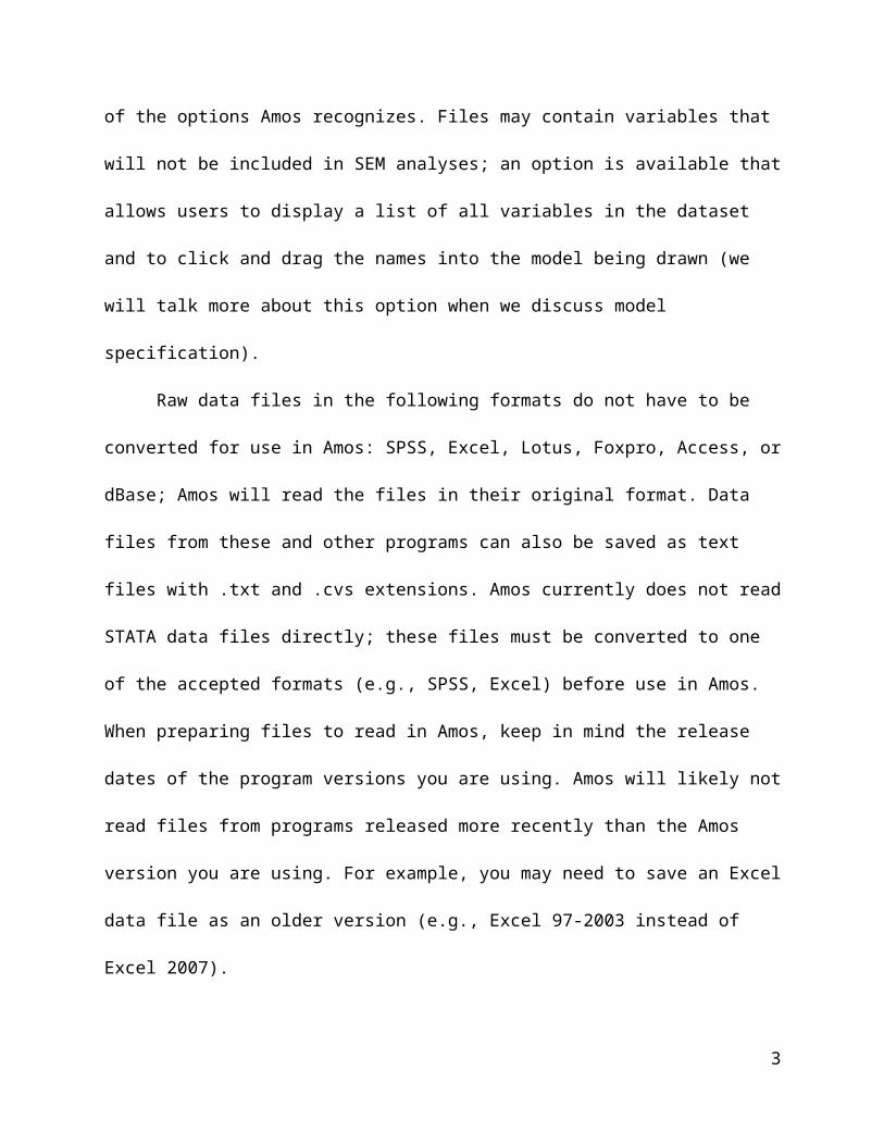
one of the options Amos recognizes. Files may contain variables that will not be included in

SEM analyses; an option is available that allows users to display a list of all variables in the

dataset and to click and drag the names into the model being drawn (we will talk more about this

option when we discuss model specification).

Raw data files in the following formats do not have to be converted for use in Amos:

SPSS, Excel, Lotus, Foxpro, Access, or dBase; Amos will read the files in their original format.

Data files from these and other programs can also be saved as text files with .txt and .cvs

extensions. Amos currently does not read STATA data files directly; these files must be

converted to one of the accepted formats (e.g., SPSS, Excel) before use in Amos. When

preparing files to read in Amos, keep in mind the release dates of the program versions you are

using. Amos will likely not read files from programs released more recently than the Amos

version you are using. For example, you may need to save an Excel data file as an older version

(e.g., Excel 97-2003 instead of Excel 2007).

When using raw data files, users should pay close attention to the variable names used in

their file. When reading data files, Amos treats the first row in the file as the variable names.

With most file types, this does not pose a problem for the user. For example, when reading SPSS

data files without user-specified variable names, Amos will keep the generic name assigned by

2

the original program to each variable (e.g., V1, V2, and so on in SPSS). With text files (e.g., .txt

or .cvs) however, users must indicate variable names in the first row of their file to avoid having

Amos treat the first row as variable names instead of actual data. Regardless of the data file type

being used, the names of observed variables used in the SEM model must match those in the

dataset exactly. For example, if Amos is reading an SPSS file with variable names Supcares and

Suphelps, the user must use those variable names when specifying that these two variables are

expected to load on a latent construct (e.g., supervisor support).

Amos can also read correlation and covariance matrices. The format required for Excel

covariance matrix files to be used by Amos is illustrated below.

rowtype_ varname_ rating weight height GPAn 209 209 209 209

cov rating 1.015

cov weight -5.243 371.476

cov height -0.468 19.024 8.428

cov GPA 0.526 -6.71 1.819 12.122

The first cell in the top row contains the column heading “rowtype_”, under which “n” signifies

that the number “209” under each variable name is the number of cases with data for the

variable, and “cov” indicates that the numeric values are covariances. The next column heading,

“varname_” indicates that the four entries below it are variable names. These four names also

appear as column headings such that the column and row variable names form a grid in which

each numeric entry refers to either a variable variance (such as, 1.015 for rating), or a covariance

between two variables (such as, 19.024 for height and weight). Note, the underscores at the end

of rowtype and varname are required!

If a correlation matrix is used as the input matrix for CFA or SEM analyses, it requires

the following format.

3

rowtype_ varname_ Raceth poverty nghsup peerbeh crimen 415 415 415 415 415corr Raceth 1corr poverty 0.44 1corr nghsup 0.08 0.07 1corr peerbeh 0.19 0.24 0.39 1corr crime 0.23 0.18 0.22 0.37 1stddev 0.483 0.466 1.56 2.03 2.07mean 0.369 0.318 1.84 1.51 1.18

Note the two important differences between covariance and correlation input matrices. First,

“corr” replaces “cov” in the “rowtype_” column. Second, the standard deviation and mean of

each observed variable is entered in the two rows at the bottom of the correlation matrix.

B.2. Specifying Data Files in Amos

Once the data file is prepared and saved in a version that Amos recognizes, we are ready

to specify the file location in Amos. The same steps are used regardless of the file type (e.g.,

SPSS or text; raw data or correlation matrix). Open Amos graphics. The opening screen as

shown in Figure 1 will appear.

See Figure 1

Go to “File Data Files…” from the pulldown menu (or click the “Select Data File”

icon, which is the 8th icon down in the first column). Then select the “File Name” button. In the

dialog box illustrated in Figure 2, select the type of file to browse for, then find, select, and

“open” the saved file. After a file has been selected, it will appear in the Amos Data File box,

along with the number of cases Amos is able to detect in the file. Users should check to be sure

the number of cases detected by Amos agrees with the number of cases known to be in the

original data file. Users can also choose “View Data” to see the actual input file.

See Figure 2

4

B.3. Model Specification in Amos

In Amos, models are specified by creating a graphical representation of the model to be

tested. In this section, we first present the basics of drawing models using the graphic tools

provided in Amos. We then we provide annotated examples of common types of CFA and

general SEM models. All work is based on version 18 of the Amos graphics program.

B.3.a. Basics of Drawing Models in Amos

The opening screen of the Amos graphics program (shown in Figure 1) includes a

drawing toolset and a blank workspace for the drawing of models. The tools are displayed as

icons on toolbars. Alternatively, the same tools can be accessed from the pulldown menus.

Simply as a matter of preference (and because they require fewer necessary clicks), the examples

we present usually refer to using the toolbar icons. Users can identify icons by moving the cursor

over them; their function will appear in text.

When drawing models, latent variables are indicated by circles, observed variables are

indicated by rectangles, and relationships between variables are depicted by one-headed or two-

headed arrows. Let’s recreate the basic measurement model in Figure 3 to practice using Amos

drawing tools. In this model, we hypothesize three latent variables (Risk1, Risk2, and Behavior),

each of which are measured by three observed variables (x1 through x9).

See Figure 3

You could use the individual circle, rectangle, and arrow tools to recreate this figure. A

more efficient approach, however, is to use the “Draw Indicator Variable” icon (at the top of the

third column), which performs several functions. Click on the icon to activate it, move the cursor

to the desired position in the drawing area, and click once to create a circle for the first

5

unobserved latent variable (as shown in Figure 4). If you prefer the circles to be larger or smaller

than the standard size used by Amos, you can click and drag the mouse pointer (rather than

simply clicking) to draw a custom size.

See Figure 4

As shown in Figure 5, clicking on the circle (with the “Indicator” icon still activated)

adds several elements to the model: (a) a rectangle (representing a single observed variable), (b)

an arrow pointing from the latent factor to the observed variable, and (c) a smaller circle with an

arrow pointing toward the observed variable (representing a measurement error term). Each

additional click of the mouse (with the Indicator icon activated), adds an additional indicator

variable and its associated error term. Error regression coefficients are automatically set to 1. The

user must fix one factor loading per factor to 1 for identification purposes. Note that Amos

automatically sets the factor loading of the first observed indicator drawn in a factor to 1. This

default can be changed by the user; we present steps to do so in Section B.3.b, Example 1.

See Figure 5

Amos automatically aligns the observed variables and their error terms above the latent

variable. We can align the observed variables to the left or right of the latent variable (as in our

hypothesized model) by using the “Rotate” function. With the “Indicator” icon activated, right

click on the latent variable and select “Rotate” from the dialog box of choices as illustrated in

Figure 6 (alternatively, select the “Rotate” icon from the toolbox—it is the 6th icon down in the

middle column). Figure 7 shows the results of this rotation.

See Figures 6 and 7

We can now repeat these drawing and rotating steps for the remaining two factors. If two

factors have the same number of indicators, as is true of all three of our factors, we can select

6

what we have drawn (using the “Select all objects” icon, 4th down in the middle column), then

click on the “Copy” icon (find the picture of the copy machine). Click any where on the current

image and drag a copy to where you want to place the second factor. If necessary, indicators can

be rotated as described above. The results are illustrated in Figure 8.

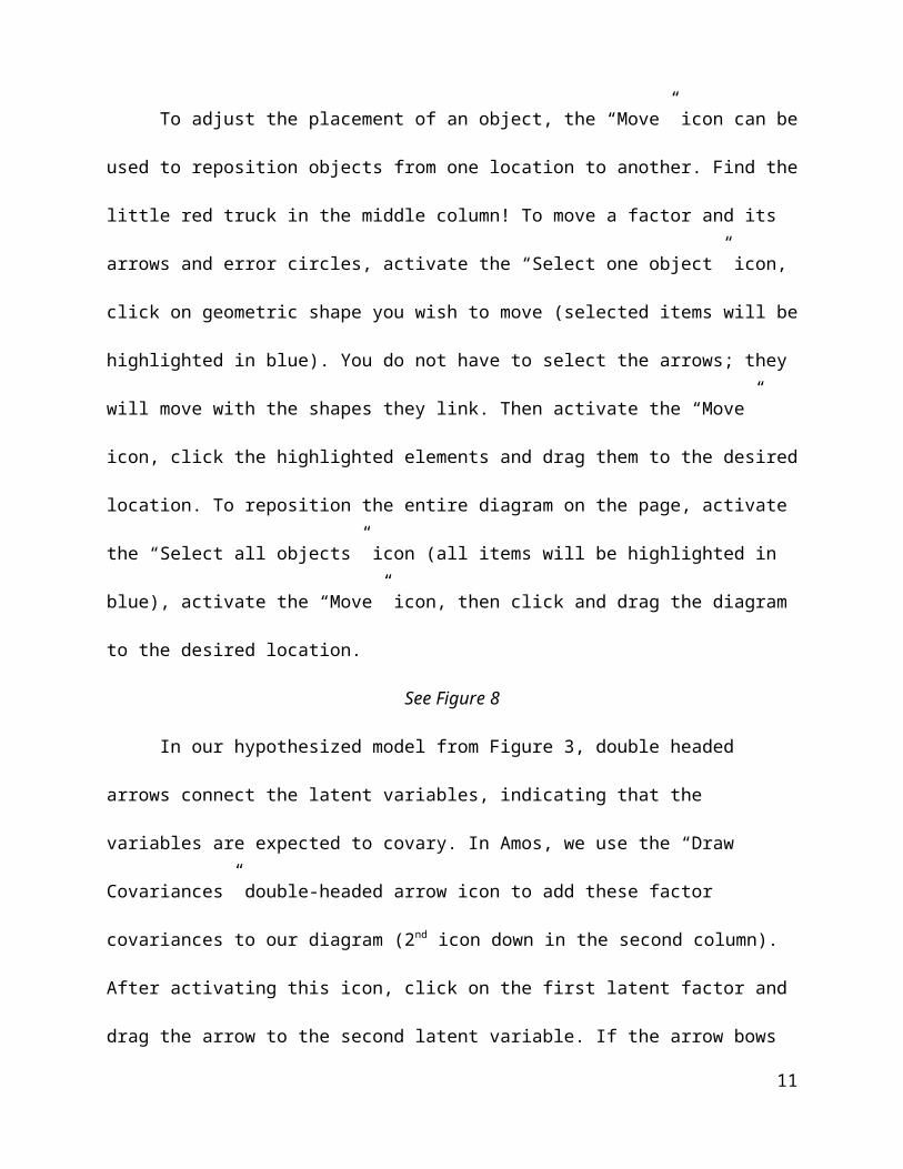
To adjust the placement of an object, the “Move” icon can be used to reposition objects

from one location to another. Find the little red truck in the middle column! To move a factor

and its arrows and error circles, activate the “Select one object” icon, click on geometric shape

you wish to move (selected items will be highlighted in blue). You do not have to select the

arrows; they will move with the shapes they link. Then activate the “Move” icon, click the

highlighted elements and drag them to the desired location. To reposition the entire diagram on

the page, activate the “Select all objects” icon (all items will be highlighted in blue), activate the

“Move” icon, then click and drag the diagram to the desired location.

See Figure 8

In our hypothesized model from Figure 3, double headed arrows connect the latent

variables, indicating that the variables are expected to covary. In Amos, we use the “Draw

Covariances” double-headed arrow icon to add these factor covariances to our diagram (2nd icon

down in the second column). After activating this icon, click on the first latent factor and drag

the arrow to the second latent variable. If the arrow bows in the opposite direction you want,

reclick and start drawing from the second factor instead. Figure 9 illustrates the results of

repeating this process for each of the remaining covariance relationships indicated in our

hypothesized model. Arrow bows (as well as circles and rectangles) can be resized (flattened or

arched in the case of arrow bows) using the 6th icon down in the first column, if desired. Note

7

that Amos is not particular about the aesthetics of your drawing. It understands the specified

model regardless of whether the graphic is publication-ready!

See Figure 9

The final step in recreating our hypothesized model is to name the variables and fix or

constrain parameters, if appropriate. When naming the observed variables (indicated with

rectangles in the model), keep in mind that the variable names must match the variable names

used in the data file to be analyzed. Although, note that Amos is not case specific. To avoid

naming errors, users can obtain a list of variables in the file to be analyzed (by activating the

“List Variables in the Dataset” icon, 3rd icon down in the third column) and drag the variable

names into the model being drawn, as illustrated in Figure 10. Naming of latent variables (factors

and error terms) can be accomplished by right-clicking on the variable, selecting “Object

Properties” from the popup dialog box (as shown in Figure 11). In the “text” tab, enter the name

(as shown in Figure 12). Font size and style (e.g., bold, italics) can also be changed if desired.

Figure 13 illustrates the final model, after repeating the naming process for each of the variables.

Note that because the latent variables (factors and error terms) are not observed items from the

data set, the user is free to choose the names. However, it is good practice to name the error

terms in such a way that the error term associated with a particular observed variable is easily

identifiable. In this example, error terms are simply named e1 through e9 to reflect the observed

indicator names of x1 through x9.

See Figures 10, 11, and 12

To fix or unfix a parameter value, go to the “parameter” tab in the “Object Properties”

box. If Amos has fixed a parameter at 1, you will see a 1 in the parameter box. Deleting the 1

indicates you want the parameter to be freely estimated. If the box is empty, indicating Amos

8

plans to freely estimate the parameter, add a 1, 0 or other value to which you want the value

fixed. If you want to constrain a parameter to be equal to the value of another parameter in the

model, enter a parameter name here and in the parameter value box for the other parameter. For

example, if you want to factor loadings to have the same value, enter “lamba1” in both boxes.

The value of lambda1 will be estimated and applied to both factor loadings.

See Figure 13

When specifying models using Amos graphic functions, it is important to remember that

relationships between variables are specified by the presence, as well as the absence, of lines

connecting them. Users must draw two-headed arrows between latent variables that are expected

to be correlated. If a possible covariance path is not included in the diagram (i.e., no line is

drawn between the variables), the covariance is presumed to be equal to zero, and this parameter

will not be estimated. For example, the absence of double-headed arrows between the

endogenous measurement errors in this example indicates that none of the errors are

hypothesized to be correlated with one another. Amos will provide a warning before analyzing a

model if any pair of exogenous variables (excluding error terms) is not specified as correlated. If

the user indicates that the lack of correlation was intended, the program will continue.

B.3.b. Examples of Model Specification

We will now look at additional examples of specifying CFA and general SEM models.

Example 1: 3-factor CFA with 9 observed variables and two pairs of correlated

measurement errors

The following model is the same type of 3-factor CFA as the model we created through

the detailed steps of the previous section. Aside from the layout of the model (factor structures

are aligned horizontally instead of the circular pattern used in the previous example), the key

9

difference is the presence of two pairs of correlated measurement errors. As described earlier, the

absence of a line connecting two variables indicates the assumption that the variables are not

correlated. In this example, the two double-headed arrows specify that the two pairs of

measurement error variances are correlated (not the variables themselves).

See Figure 14

By default, the loading of the first indicator of a factor is fixed at one and error paths are

fixed at one. To change the default setting of the first loading of JOBSAT, right-click on the

arrow representing the first factor loading and select “Object Properties” from the menu, and

click on the “Parameters” tab within the dialog box (as illustrated in Figure 15). Delete the 1 in

the regression weight box to remove the default loading. Now open the same dialog box for the

factor loading you desire to fix at one, and enter a 1 in the regression weight box. To set the

metric of JOBSAT by fixing its variance to 1 instead of one of its loadings, a similar process is

used. Simply remove any existing factor loadings that are fixed to 1 by following the process just

described. Then right-click on the latent variable JOBSAT, select “Object Properties” from the

menu, click on the “Parameters” tab, and enter a 1 in the variance weight box.

See Figure 15

Example 2: Second-order CFA

We now hypothesize a higher order factor “Work Experience” as accounting for, or

explaining, the variance and covariance related to the first-order factors of JOBSAT,

LIKESUPR, and JOBCOMM.

See Figure 16

The easiest approach to creating this new second-order model is to start from our

previous first-order model (from Figure 14). Rename the graphics file if you want to keep the

10

original model. The structure of JOBSAT, LIKESUPR, and JOBCOMM will remain the same.

The factor covariances connecting these variables (i.e., the double-headed arrows) can be

removed by using the “Erase Objects” icon (the red X). Activate this icon, then click on each of

the double-headed arrows connecting the latent variables to delete them (we will keep the

correlated error terms). In Figure 17, the covariance between LIKESUPR and JOBCOMM has

been deleted; the covariance between LIKESUPR and JOBSAT is being deleted.

See Figure 17

With these factor covariances removed, we are now ready to draw a circle representing

the new second-order latent variable for “Work Experience” – WORKEXP – and the regression

paths between this variable and the first-order variables. Click on the “Draw Unobserved

Variable” icon (i.e., the blue oval), move the cursor to the location in the drawing area where you

would like to place the variable, and left-click to place the shape. Then, activate the “Draw

Paths” icon (i.e., the single-headed arrow) to draw regression paths between the second-order

factor and each of the three first-order latent variables. Figure 18 illustrates the drawing process.

The second-order latent variable (WORKEXP) is named using the same process as before.

See Figure 18

Remember that model identification requires a constraint to be placed on either the

variance of a latent variable or one of its regression paths. Because we are using the individual

“Draw Unobserved Variable” icon, Amos does not automatically add this constraint for us; we

must add it manually. In second-order CFA models, the relationship (i.e., regression path)

between the second-order factor and each of the first order factors is usually of greater interest to

the researcher than the variance of the second-order factor. For this reason, the variance of the

second-order factor is usually constrained (to 1), leaving the factor loadings (i.e., regression

11

paths) open to be estimated. As in earlier examples, we can right-click on the WORKEXP

variable, select “Object Properties” from the menu, click on the “Parameters” tab, and enter a 1

in the variance box.

Each of the first order variables (JOBSAT, LIKESUPR, JOBCOMM) is now a dependent

variable in the model; therefore, we need to add a residual error term for each variable to indicate

the error of prediction of the variable by the higher order WORKEXP variable. To do so, activate

the “Add a Unique Variable” icon (2nd icon down in the third column), then click on one of the

first-order latent variables. Amos will add the error term directly above the latent variable.

Additional clicks of the mouse will move the placement of the error term by rotating it 45

degrees around the latent variable. Figure 19 illustrates the results of repeating this process for

each of the first-order latent variables.

See Figure 19

For model presentation purposes, however, the user may not like that Amos has

overlapped the error term for LIKESUPR with the regression path between WORKEXP and

JOBSAT. The size and placement of these error terms (as well as any model element) can be

fine-tuned using the “Change Shape of Objects” and “Move Objects” icons. To fine-tune the size

of all three error terms simultaneously, activate the “Select One Object” icon, click on each of

the three error term circles (outlines will turn blue when selected), then click on the “Change

Shape” icon to activate it. Alternatively, the user may resize these objects individually by only

selecting one error term instead of all three. To fine-tune the placement of the error terms, select

one (or all) of the error term circles, activate the “Move Objects” icon, then left-click and drag

on error term circle to the desired location. Figure 20 shows the results of resizing the error term

circles and Figure 21 illustrates the results of moving the circles.

12

See Figures 20 and 21

The last step in creating the model is naming the newly added residual error terms. Recall

that this is done by right-clicking on the object, selecting “Object Properties” from the popup

dialog box, selecting the “Text” tab, and entering the desired name for the variable. The full CFA

model is illustrated in Figure 22.

See Figure 22

Example 3: Multiple Group CFA

A measurement model (or General SEM) can be tested to see if it is “invariant” across

groups. Additional steps are required in the data file selection and model specification steps.

Multiple group instructions vary depending on a number of variable and model issues. The

example presented here is simple. Readers are referred to the Amos User’s Guide for more

information.

In this example, we want to test whether the second-order measurement model from

Example 2 is the same for men and women. To do so, we begin with the graphic of the model we

created in Example 2. We first indicate the data file we will use (“Exceldemo2-sheet1.xls”). This

file contains all of the data for both male and female respondents. As illustrated in Figure 23, we

see that there is one group listed “Group number 1” and there are 558 cases in this data file.

See Figure 23

To form the two groups of interest (male and female), go to the “Analyze” pulldown

menu and select “Manage Groups” as shown in Figure 24. As we saw when specifying the data

file, there is one group listed (Group 1). Rename this group “Males.” Click on “New” to add a

second group (Group 2). Rename this group “Females”.

Place Figures 24 and 25

13

Go to the “Data File” dialog box. As displayed in Figure 25, two groups should now be

listed – Males and Females. Select one group at a time and indicate the data file you plan to use

for the analysis, the variable from the data file that will be the grouping variable, and the value of

the grouping variable. In this example, the data file (“Exceldemo2-sheet1.xls”) and grouping

variable (“gender”) will be the same for both groups, but Amos does allow you to select different

options for each group. Using the “Group Value” button, specify the coding that Amos should

use to identify the two groups. In our example, the grouping variable “gender” is a dichotomous

variable, and the “group values” are coded as 0=women and 1=men. Figure 26 illustrates the data

file box after these steps are completed. There are now two groups defined by the variable

“gender”: 252 females and 303 males. (From these totals, we note that three cases are missing

data on the gender variable. Therefore, we will need to accommodate this fact when estimating

our model; this task is described in the section on Analysis Properties.)

See Figure 26

Note that the uppermost box in the center of the Amos display (indicated by the arrow in

Figure 26) now lists Males and Female. Although we have only drawn one picture, Amos made

two copies – one for each group. By placing no constraints on the two pictures, we are allowing

Amos to estimate all of the free parameters in the model separately for each group. This is the

least restrictive model (Amos will estimate all free parameters separately for each group) – we

will refer to this model as Model A. When we run the model with no constraints, the fit indices

provided by Amos will apply to the whole model, but parameter estimates will be generated

separately for each group.

14

Now we are ready to test for measurement invariance – that is, if the measurement model

is the same for men and women. To let Amos know that we want to constrain estimates to be

equal across groups, we have to name the parameters we want to constrain. Following the

hierarchy for testing model invariance (as described in Chapter 7), we first constrain each of the

factor loadings (i.e., the lambda’s) to be equal for men and women by labeling the lambda

parameters with the same “value” for both groups. We do so by writing a name in the “regression

weight” box as shown in Figure 27. By applying this one name to a particular factor loading for

both groups, Amos understands that we want the estimate for that particular parameter to be

constrained to be equal across the groups. Note that we only need to label the factor loading for

one group. There is a small box for “all groups” that is checked by default. Unless we uncheck

that box, any label or value we give a parameter will be applied to the same parameter in all

groups.

See Figure 27

With each constrain of the factor loadings (lambda’s), we can run the model, determine

the chi-square and degrees of freedom values, and conduct a chi-square difference test to

determine if model fit got significantly worse when we constrained the lambda’s to be equal

across the two groups. We would be comparing the fit of Model A (the least restrictive model,

which is our initial model without constraints) and Model B (the more restrictive, or constrained

model). If we determine that model fit did not get significantly worse, we proceed through the

hierarchy of constraints (as described in Chapter 7), specifying and testing models that

increasingly constrain the model to be equal across the two groups.

Example 4: General SEM

15

Most aspects of model specification are the same for general SEM as for CFA. Second-

order and multiple group analyses can be conducted. The model pictured below in Figure 28 is

based on the measurement model used in the previous examples. In this model we hypothesize

two latent variables JOBSAT and LIKESUPR (each measured by three observed indicators)

predict overall JOBCOMM (a third latent variable that is measured by three observed indicators).

Note that the structural part of the model is just-identified (df =0). In a real study, we would have

to address this issue in order to test the hypothesized relationships among latent variables.

Example 5 below shows one way we could resolve this issue and make the model over-

identified.

See Figure 28

No new skills are needed to recreate this model in Amos – you can simply apply the

drawing and model specification skills from the previous examples. You may choose to start

from a blank Amos drawing screen. Alternatively, you may choose to start with the measurement

model we created in Example 1 because very few changes are required to transform it into this

SEM diagram. Beginning with an existing diagram will also provide valuable practice in using

the “Delete,” “Select,” “Rotate,” and “Move,” tools. Figure 29 illustrates the results of using the

delete, select, rotate, and move tools to rearrange elements from Example 1; these elements will

now form the basis of our SEM model diagram.

See Figure 29

With these elements in place, we can add lines to specify the hypothesized relationships

between our latent variables. We add a double-headed arrow to specify a hypothesized

covariance between JOBSAT and LIKESUPR. We then use the “Draw Path” icon to add two

single-headed arrows to signify hypothesized regression paths – one path connects JOBSAT and

16

JOBCOMM, and a second path connects LIKESUPR and JOBCOMM. Unlike in our earlier

CFA model in Example 1, JOBCOMM is now modeled as a dependent variable, and therefore

must have an associated residual error term. As in earlier examples, we use the “Add Unique

Variable” icon to add this error term and the “Object Properties” dialog box to name it. Figure 30

illustrates the results of these steps.

See Figure 30

Example 5: General SEM with Latent and Observed Predictors

As illustrated in Figure 31, the inclusion of gender as a predictor of JOBCOMM makes

the structural part of the model over-identified. Amos knows GENDER is an observed variable

because it is drawn as a rectangle and given the name of one of our observed variables. Likewise,

Amos knows that GENDER is hypothesized as a predictor of JOBCOMM because we drew a

regression path (i.e., a one-headed arrow) connecting the two variables. Note that if we run the

model as pictured in Figure 31, Amos will remind us that GENDER is not correlated as expected

with JOBSAT and LIKESUPR.

See Figure 31

Example 6: General SEM with Latent Predictors, Observed Predictors, and Mediation

In the following SEM, we hypothesize a mediation pathway. As in the model from

Example 5, both JOBSAT and LIKESUPR have direct effects on JOBCOMM. New to this

model is the hypothesis that LIKESUPR has a direct effect on JOBSAT, and therefore,

LIKESUPR has an indirect effect on JOBCOMM through its direct effect on JOBSAT. To model

these hypothesized effects, the double-headed arrow (i.e., covariance relationship) between

JOBSAT and LIKESUPR has been deleted and replaced by a single-headed arrow, representing

the hypothesized direct effect of LIKESUPR on JOBSAT. Now that JOBSAT is being modeled

17

as an endogenous variable (predicted by LIKESUPR), it has an associated residual error term. As

in earlier examples, we use the “Add Unique Variable” icon to add this error term and the

“Object Properties” dialog box to name it. Figure 32 illustrates the results of these steps.

See Figure 32

B.4. Basics of Defining Analysis Properties in Amos

As described earlier, the process of testing CFA and SEM models in Amos involves two

key steps: (a) specifying the model by drawing a graphic representation of the relationships to be

tested and (b) defining the specific analyses to be used to test the model. The previous section

provided several examples of specifying various CFA and SEM models. In this section, we

present the basics of defining analysis properties. Users can access the “Analysis Properties”

dialog boxes by clicking “ViewAnalysis Properties” from the pulldown menus or by selecting

the “Analysis Properties” icon from the toolbar. As illustrated in Figure 33, the Analysis

Properties dialog box contains several tabs: Estimation, Numerical, Bias, Output, Bootstrap,

Permutations, Random #, and Title. Amos provides numerous options for model analysis – only

the basics of selecting model estimation methods, handling missing values, and specifying output

options are presented here. Readers are referred to the Amos User’s Guide for more detailed

information on the many Analysis Properties options available.

See Figure 33

Model Estimation: The Estimation tab (illustrated in Figure 33) of Analysis Properties

provides several model estimation options. Maximum likelihood is the default estimator.

Variables with non-normal distributions can be analyzed with the Asympototically distribution-

free estimator (ADF). Although SEM experts disagree on the adequacy of the ADF estimator,

there seems to be some consensus that with very large samples (over 1000 cases) the ADF may

18

perform well, but not with smaller samples. The Numerical tab allows the user to adjust the

default convergence criteria and iteration limits if a model has trouble converging.

Missing Data: The Estimation tab allows the user to specify that the data file to be

analyzed has missing data. When the data file to be analyzed has missing values, the user must

select the “estimate means and intercepts” option. Amos will provide a warning if the data file

has missing values and the user fails to specify this option. Amos does not provide modification

indices when the “means and intercepts” option is used, even if the user requests them.

Specifying Output Options. The Output tab of Analysis Properties (illustrated in Figure

34) allows the user to customize the output provide by Amos. Based on model evaluation steps

discussed in this book, we recommend requesting standardized estimates, squared multiple

correlations, residual moments, and modification indices (if there are no missing values).

See Figure 34

B.5. Calculating Estimates and Accessing Output

After drawing the hypothesized model and specifying analysis options, the user is ready

to analyze the model. To do so, select “AnalyzeCalculate Estimate” from the pulldown menu

or select the “Calculate Estimates” icon from the toolbar (the 8th icon down in the third column,

as illustrated in Figure 35).

See Figure 35

Amos will run the calculations and display an analysis summary in one of the boxes in

the center of the screen (highlighted by the arrow in Figure 36). Amos creates a copy of the

model picture with the parameter estimates – click the “View the Output Path Diagram” button

(the box under and between “Analyze” and “Tools” in the Menu line). This button is activated in

Figure 36. You may use the button (along with the “View the Input Path Diagram” button to the

19

left of it) to toggle between the input (model specification) and output (parameter estimates) path

diagrams. Additionally, the user may toggle between unstandardized and standardized estimates

by highlighting the appropriate text in the third white box down from the Input and Output Path

Diagram buttons. Full output can be accessed by clicking “ViewText Output” from the

pulldown menu or by selecting the “View Text” icon from the toolbar. Amos will open a new

window in which the full text output will be displayed. From this new window, the user may

browse the output, print, or save the output to a file.

See Figure 36

20

Figure 1. Amos Opening Screen

Figure 2. Selecting Data Files in Amos

21

Risk1

X33

11

X22

1

X11

1

Risk2

X66

11

X55

1

X44

1

X7 7

11

X8 8

1

X9 9

1

Behavior

Figure 3. Basic Measurement Model

Figure 4. Drawing a circle to represent an unobserved variable

22

Figure 5. Adding the first observed indicator and error term to the latent variable

Figure 6. Selecting the “rotate” function from the pop-up dialog box

23

Figure 7. Results of rotating the factor structure layout

Figure 8. Adding the remaining two factor structures

24

Figure 9. Drawing the factor covariance double-headed arrows.

Figure 10. Using list of variables in data set to name observed variables in model

25

Figure 11. Selecting the “Object Properties” option from the popup menu.

Figure 12. Using the “Object Properties” dialog box to name latent variables in the model

26

Figure 13. Hypothesized model from Figure 3 fully replicated in Amos

Figure 14. Three-factor CFA with two pairs of correlated error terms

27

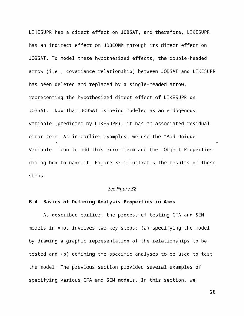
Figure 15. Using object properties to set a factor loading

Figure 16. Second-order CFA model

28

Figure 17. Deleting the factor covariances (double-headed arrows)

Figure 18. Adding a second-order factor and its associated regression paths.

29

Figure 19. Using the “Add Unique Variable” icon to add error terms to each first-order variable

Figure 20. Using the “Change Shape of Objects” tool to resize error term circles

30

Figure 21. After fine-tuning size and placement of error terms for each first-order latent variable

Figure 22. Hypothesized Measurement Model Fully Depicted in Amos

31

Figure 23. Data File Dialog Box

Figure 24. Selecting “Manage Groups” to Form Multiple Groups from our Data Set

32

Figure 25. Two Groups Listed in the Data File Dialog Box

Figure 26: Multiple groups defined, with file names and group values

33

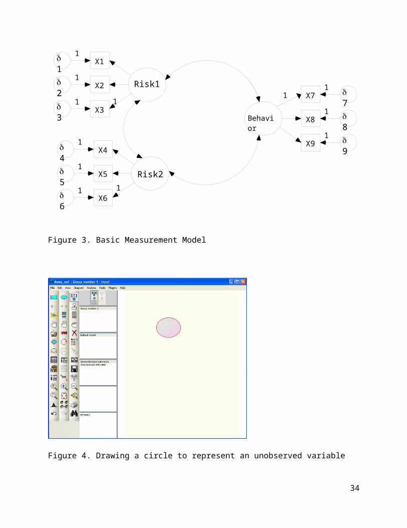
Figure 27. Constraining Factor Loadings to Be Equal Across Groups

Figure 28. Hypothesized General SEM Model

34

Figure 29. Using Elements of Example 1 to Create a New SEM diagram

Figure 30: Specifying a General SEM model in Amos

35

Figure 31. General SEM with Latent and Observed Predictors

Figure 32. General SEM with a Mediation Hypothesis

36

Figure 33. Accessing the “Analysis Properties” dialog boxes

Figure 34. Output Options

37

Figure 35. Selecting the “Calculate Estimates” icon from the toolbar

Figure 36. Viewing the Output Path Diagram after Running the Model

38