Embed Size (px)
Citation preview
High-end Encroachment Patterns of New Products
Bo van der Rhee*
Nyenrode Business University, Breukelen, The Netherlands
Glen M. Schmidt
David Eccles School of Business, University of Utah, Salt Lake City, UT 84103
Joseph Van Orden
West Point Military Academy, West Point, NY 10996
*Corresponding authorPhone number: +31 346291745Fax number: +31 346291250

High-end Encroachment Patterns of New Products
ABSTRACT
Previous research describes two key ways in which a new product may encroach on an existing
market. In high-end encroachment the new product first sells to high end customers and then
diffuses down-market; in low-end encroachment the new product enters at the low end and
encroaches up-market. This paper extends the framework for high end encroachment: 1) we
gain insight into market outcomes under three distinct high-end encroachment sub-types; and 2)
we offer a detailed numerical example to illustrate how our findings might be used to explain
actual market outcomes. Our example concerns the sub-type we call new-market high-end
encroachment, in which a new product initially sells at a high “monopoly” price without
affecting the sales of the original product, and then diffuses (encroaches) down-market. We
offer possible insights into why Apple precipitously dropped the price of the iPhone by 1/3 only
68 days after its introduction.
Keywords: Encroachment, Linear Reservation Prices, New Product Development
1. INTRODUCTION
Previous research has suggested that a new product might encroach on (take market share from)
an old product market in one of two key basic ways (possibly after the new product first opens
up a new market of its own); either the new product1 first sells at a relatively high price at the
high end of the market and then encroaches down-market (a process called high-end
encroachment – an example is the Pentium IV encroaching on the Pentium III), or the new
product first encroaches on the low end of the old-product market and then encroaches up-market
(low-end encroachment – an example is Southwest Airlines encroaching on Continental
1 We use the term “product” generically, i.e., our findings can apply to services as well as physical products.
1
Airlines). See Schmidt and Porteus (2000) and Schmidt (2004). Other previous works delved
further into the low-end encroachment process, suggesting there are multiple ways that low-end
encroachment could occur (see Schmidt and Druehl 2008; and Druehl and Schmidt 2008).
Finally, Van Orden et al. (2010) empirically validates the encroachment framework.
Our paper focuses on high-end encroachment, subcategorizing it into three sub-types,
which we derive herein using a linear-reservation price curve model (LRPCM). In § 2 we
delineate and lend insight into these three high-end subtypes, denoted by the “immediate,” “new-
attribute,” and “new-market” scenarios. With the immediate type the new product immediately
encroaches on (i.e., takes sales away from) the old product at the high end. The previously-
mentioned example of the Pentium IV encroaching on the Pentium III fits this category. With
the new-attribute type the new product has enhanced features to the extent that it not only
competes with the existing product at the high-end of the “original” market but it also attracts
new high-end customers. An example of this type of product is the pain killer naproxen (better
known as Aleve) – while it can be used for headaches, as compared to aspirin it adds a new
feature, that of being an anti-inflammatory agent. Finally, in the new-market type, the new
product is different (desirable) enough that it first opens up a new high-end market. As such, the
new product commands significant (“monopoly”) pricing power in the new market and first sells
only to these customer, while over time it may eventually encroach on the original product from
the high end downward, or fizzle out after a brief ´fad´ period.
The LRPCM2 provides the basis for extending the framework of high-end encroachment
to its three sub-types. It illustrates market outcomes when a new product is introduced into a
market, as a function of the new product’s attributes and characteristics relative to those of the
original product. Specifically, the LRPCM identifies the market segments to which the new
2 While we suppress the analytics to the technical appendices, we discuss the findings in § 2.
2
product and the competitive original product are sold, along with sales prices, sales volumes, and
market shares.
Another contribution of our paper is to offer a detailed numerical example to illustrate
how our LRPCM might be applied; using in § 3 the example of Apple’s iPhone. We discuss and
show how it epitomizes the new-market high-end encroachment type, the type that has not
received much attention in the literature to date. While we do not claim that our stylized model
fully explains all the dynamics of Apple’s competitive environment, it lends insight into why
Apple precipitously dropped the price by one third after only 68 days on the market. Other
products that have likewise experienced a fast-paced drop in price shortly after introduction
include the Razr phone, the Razor scooter, TiVo, the Furby, and the DVD-L10, the first portable
DVD player, by Panasonic. Finally, in § 4 we summarize by discussing another example, the
Tesla electric automobile.
2. APPLICATION OF THE LRPCM TO HIGH-END ENCROACHMENT
Our model is intended to parsimoniously describe how a new product might impact an existing
market over time (if at all). Our setup directly follows that of Schmidt and Porteus (2000) and
Schmidt and Druehl (2005), except as noted at the end of § 2.1. We start by assuming there is a
single original product O in a single market sold by a single firm O. A customer’s reservation
price for the product is the most that she is willing to pay for that item. We assume a customer’s
“type” is determined by her reservation price and assume reservation prices are uniformly
distributed from zero willingness to pay to some maximum greater than zero. This means that if
all customers are ordered along the x-axis according to type, from highest willingness to pay
down to the lowest, the resulting reservation price curve (RPC) can be approximated by a
continuous straight line; hence the term linear reservation price curve, or LRPC (see Figure 1).
3
We use the term “customer” to mean all persons who have a positive reservation price
(not all customers will actually buy the product; the purchase decision is described below).
Customers with the highest reservation prices are called high-end customers, while the lower-end
customers have lower reservation prices.
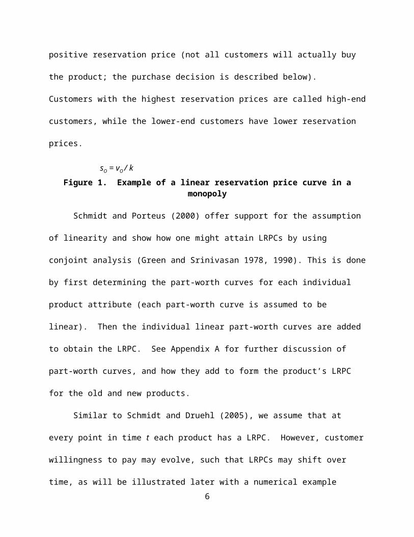
Figure 1. Example of a linear reservation price curve in a monopoly
Schmidt and Porteus (2000) offer support for the assumption of linearity and show how
one might attain LRPCs by using conjoint analysis (Green and Srinivasan 1978, 1990). This is
done by first determining the part-worth curves for each individual product attribute (each part-
worth curve is assumed to be linear). Then the individual linear part-worth curves are added to
obtain the LRPC. See Appendix A for further discussion of part-worth curves, and how they add
to form the product’s LRPC for the old and new products.
Similar to Schmidt and Druehl (2005), we assume that at every point in time t each
product has a LRPC. However, customer willingness to pay may evolve, such that LRPCs may
4
High-end customers
Low-end customers
pO
Quantity sold
ProfitpO
Customers who
purchaseCustomers who do not purchase
Customer type, x
Res
erva
tion
pric
e
0 qO
cO
vO
sO = vO / k
shift over time, as will be illustrated later with a numerical example (Figure 2 and in § 3). We
denote the time of introduction of the new product as time t = 1 (e.g., on “day 1”).
Continuing to refer to Figure 1 (in the figures we omit the time dependencies to reduce
clutter), the per-unit cost of product O at time t (assumed to be constant over volume) is denoted
by cO(t), its maximum reservation price is denoted by vO(t), and the negative slope of its LRPC is
denoted by k(t), such that the x-axis intercept, indicating the total potential the size of O’s market
is sO(t) = vO(t) / k(t). Define mO(t) ≡ vO(t) – cO(t), indicating the maximum potential markup for
product O (marking it up by this amount guarantees zero sales). The firm is assumed to
myopically set price pO(t) to maximize the rate of profit generation (considering only the current
reservation prices and costs), where the profit rate is the sales rate qO(t) (i.e., the number of units
sold per unit time) multiplied by the per-unit margin (i.e., price minus cost). The profit rate pO(t)
is represented by the dark area in Figure 1. If O is the only product in the market, then the LRPC
is akin to a linear demand curve.
2.1. Introduction of the New Product
In Figure 2 we show the case where a second firm N has introduced a new product N to compete
with O. In this paper we deal with the case of high-end encroachment, which Schmidt and
Porteus (2000) show to result when the reservation price curve for the new product is steeper
than that of the old product. See Appendix A for further details as to why high-end
encroachment is represented by the case where product N’s LRPC has a steeper slope. The basic
intuition is that high-end encroachment reflects the case where the new product is enhanced
along the core performance dimension(s) of the old product, and in addition, it offers some new
(or ancillary) feature(s) that high-end customers appreciate. Thus the old product’s highest-end
customers have an elevated willingness to pay for the new product as compared to the old. On
5
the other hand, the old product’s lower-end customers are those who (by definition) don’t highly
value the core attribute performance, and who may even be alienated by the new attribute (for
example, see Van der Rhee et al. 2010 for a discussion of how low-end customers in the Xbox
gaming system market were alienated by elaborate multi-function controllers). We normalize
the x-axis intercept and the steeper slope of product N’s curve to one, such that the slope of the
curve for the original product is 0 < k(t) < 1. Notation for parameters related to product N follow
those for O, e.g., pN(t) is product N’s price at time t.
Figure 2. Example of linear reservation price curves in a duopoly
In addition to being highly preferred by existing high-end customers, the new product
may be enhanced to the point where it attracts some customers into the market at the high end
who were not previously considering the old product. That is, referring to Figure 2, we extend
product N’s LRPC at the high end (to the left) by some amount e(t) ≥ 0. Effectively, we assume
that the new product attracts some new customers who are even higher-end than the highest-end
6
Res
erv a
tion
pric
e
pN
Customer type, xNew market
sO = vO / k
e
vN
1
1
cN
xN xO
y-axis of the original market(y-axis of Figure 1)
00-e }
pO
pN
qN qO
original-product customers. These are for example high-end early adopters (see e.g., Rogers
1995) who were not interested in the original product but who are interested in the new product
given that it not only offers enhanced performance along the old core dimension but also offers
strong performance along a new attribute dimension. In effect, these new-market high-end
customers (who lie along the x-axis between –e and 0 in Figure 2) had latent (dormant)
willingness to pay that was “brought to life” with the new attribute performance offered by the
new product (see Appendix A for further discussion). In § 2.2 to § 2.4 we discuss how the
market expansion is related to the type of high-end encroachment observed. Under this setup,
product O is not in the consideration set for purchase by any of the new-market customers (those
between –e and 0 in Figure 2), but we assume that product N may be in the consideration set for
purchase by some (or all) of the original customers (i.e., N’s LRPC may extend into O’s
customer base and have an intercept anywhere along the x-axis). Appendix A offers a more
detailed development of the linear reservation price framework using part-worths for the core
attribute performance of the old product and the new (and core) attribute performance of the new
product.
A product’s design effectively establishes its LRPC and its cost; thus we take these to be
exogenous parameters. Of course, before introducing a new product, a firm may want to explore
the implications of introducing various new designs, for which the LRPCs and costs, and
therefore the market outcomes, would differ. Given the LRPCs and costs at any given point in
time, each firm is assumed to set the price to maximize profit, given the competitive firm’s price
(this is the standard Nash equilibrium). If there is a customer who is indifferent between buying
O and N (i.e., has the same surplus for O and N), we denote such customer type by xN(t)
(continue to refer to Figure 2).
7
We assume a customer buys only the product offering the highest positive surplus, where
surplus is the difference between reservation price and sales price (if neither product has a
positive surplus the customer buys nothing) – the customer purchases at a rate of one unit per
time period (Norton and Bass 1987 similarly model purchase as a rate) . Since the LRPC for
product N is steeper than that for O, customers who are higher-end than xN(t) will have a higher
surplus for N and thus buy N. The customer having zero surplus for O is denoted by xO(t).
Customers in the interval between xN(t) and xO(t) will buy O while customers who are lower-end
than xO(t) buy nothing. In the example of Figure 2, N sells to the new market and to high-end
customers in the original market, and O is relegated to selling to the lower-end customers in the
original market.
This setup is equivalent to Schmidt and Porteus (2000) except that the market for product
N is extended at the high end by the amount e(t) ≥ 0 (and we focus strictly on the case where
product N’s LRPC has a steeper slope than that of product O). Also, we allow the LRPC
parameters and costs to be a function of time t (in doing so we directly follow the setup of
Schmidt and Druehl 2005). This setup results in a total of five possible market outcomes (in
order of impact on the sales for the original product): 1) dual monopolies (N sells as a
monopolist in the new market only, and O sells as a monopolist in the original market only);
2) super monopoly (N prices above the monopoly price and covers the entire new market while
O sells as a monopolist in the original market); 3) expanded differentiated duopoly (N covers the
new market and the high end of the original market while O sells in the original market);
4) constrained monopoly for N, (only N realizes any sales, but cannot price as a monopolist
because if it did O would get some sales); and 5) monopoly for N (only N realizes any sales,
8
pricing as a monopolist with O getting no sales). See Appendix B which provides the analytical
details covering these five outcomes.
Note that among the above five outcomes there are exactly three possibilities regarding
who initially buys the new product. First, the new product may sell only to customers in the new
market – this outcome we refer to as new-market high-end encroachment. Second, the new
product may sell to the new market plus the end-high customers in the original market – we refer
to this as new-attribute high-end encroachment. A third case is the special case where the
market expansion is minimal (effectively zero) – that is, there is no new market. We refer to this
as immediate high-end encroachment since the new product immediately takes the high end of
the original market. In all three cases, the new product may diffuse down-market over time from
this initial starting point. We next discuss each of these three scenarios in more detail.
2.2. Immediate High-End Encroachment: Differentiated Duopoly, e(t) = 0
The immediate form of high-end encroachment is effectively presented in Schmidt and Druehl
(2005), so we discuss it only briefly. Under this scenario, at the introduction of the new product,
we find a differentiated duopoly with e(t) = 0 (the market is not expanded on the high-end). If
the new product is highly successful, then over time customers perceive it more favorably
(enhancing its LRPC) and its cost may come down due to learning effects, for example. These
changes will result in a diffusion of the new product down-market – for example the Pentium IV
chip encroached down-market over time and eventually entirely displaced the Pentium III. In
theory, there is even the possibility that the new product is so superior that it achieves a
constrained monopoly or monopoly right away upon introduction (a firm may introduce a new
product and simultaneously drops production of the original). Given that upon introduction the
9
new product “steals” some of the original product’s high-end customers, the encroachment is
immediate (hence the name of this scenario).
2.3. New-Attribute High-End Encroachment: Expanded Differentiated Duopoly, e(1) > 0
If the new product is not only enhanced along the core dimension but also includes a new
dimension targeted at new high-end customers, then it has the opportunity to expand the market
at the high end, leading to e(1) > 0. If the new product also continues to attract current high-end
customers it competes with the original product in an expanded differentiated duopoly, yielding
encroachment of the new-attribute high-end type.
Sales of original
Sales of original
Sale
s of o
rigin
al
Sale
s of n
ew
Sale
s of n
ew
Sales of
new
Customer type Customer type Customer typeHigh-end High-end High-endLow-end Low-end Low-end
Res
erva
tion
pric
e
Res
erva
tion
pric
e
Res
erva
tion
pric
e
a) The new product is introduced and attracts existing as well as new high-end customers (i.e. it expands the market slightly).
b) The new product improves over time and sells to more high-end customers, even though some low-end customers still like the original product better.
c) The new product dominates, and only a small segment of the lower-end customers still like the original product better.
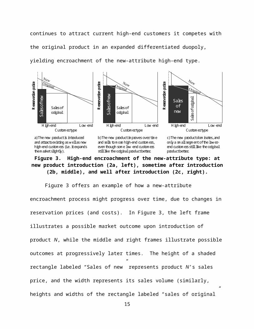
Figure 3. High-end encroachment of the new-attribute type: at new product introduction (2a, left), sometime after introduction (2b, middle), and well after introduction (2c, right).
Figure 3 offers an example of how a new-attribute encroachment process might progress
over time, due to changes in reservation prices (and costs). In Figure 3, the left frame illustrates
a possible market outcome upon introduction of product N, while the middle and right frames
illustrate possible outcomes at progressively later times. The height of a shaded rectangle
labeled “Sales of new” represents product N’s sales price, and the width represents its sales
volume (similarly, heights and widths of the rectangle labeled “sales of original” denote prices
and volumes for product O). Upon introduction (left frame “a”) the new product expands the
10
market at the high end, and sells to some new customers who were not in the market for the
original product but who now consider a purchase solely because of the new product’s
performance along the new attribute dimension. Over time (progressing to frame “b” and then
frame “c”), the original customers may view the new product more favorably, as it improves in
performance, comes down in cost, and/or as customers become more educated as to the benefits
of the new product. Thus the new product diffuses down-market as shown in the progression in
Figure 3 from the left frame to the middle frame to the right frame.
While the LRPCs cross in Figure 3, implying that the low-end customers actually ascribe
higher utility to the original product than the new, this need not be the case: our model also
applies to the situation where the LRPC for the new product lies entirely above that of the
original product or crosses even earlier (i.e., more to the left along the x-axis).
2.4. New-market High-end Encroachment: Dual Monopolies or Super-monopoly/Monopoly
New-market high-end encroachment describes the case where we find either dual-monopolies or
the super-monopoly upon introduction of product N., i.e., there exists a “new market” for product
N. As illustrated in § 3 with the iPhone example, what may (but does not necessarily) happen
with this new-market scenario is that over time it may fully cover (saturate) the new market, and
then begin to take sales away from the old product and diffuses down market. This occurs as the
new product’s cost decreases due to learning effects, and/or as customer perceptions of product
N improve relative to perceptions of product O (e.g., due to improvements in the new product
over time, proof-of-performance, externality effects, or simply perception). With continual cost
reductions and/or changes in perception the outcome may transition from dual monopolies to a
super-monopoly/monopoly, to an extended differentiated duopoly, to a constrained monopoly for
the new product, to a monopoly.
11
Alternatively, we may find that the diffusion stalls at some point. We may even find that
the substitution process (of the new product for the original) never even gets started; the new
product “fizzles out” before achieving any sales in the original market (Van Orden et al. 2010
call this as a “fad” product).
In the next section we first briefly discuss examples of products that follow the new-
market high-end encroachment pattern, before we take a closer look at how our model deals with
a recent example, the iPhone. In § 4 we discuss an example that is playing out at the time of
writing of this article, to show how our insights can assist during the product development phase.
3. EXAMPLES OF NEW-MARKET HIGH-END ENCROACHMENT
3.1. Prices Start High, Then at Some Point Drop Dramatically
In 2000 the J.D. Corporation introduced a small, thin, lightweight, and collapsible scooter
balanced on roller blade type wheels. This sleek mode of transportation glided at the speed of
rollerblades without requiring the removal of one’s shoes, and it contained the additional
advantage of not being as bulky as a bicycle. It won the prestigious Toy of the Year award from
the Toy Industry Association and in 2000 these scooters were the must-have items desired by all
cool kids, at a price between $99 and $149. A few short years later, in a completely different
industry, phones were being bulked up with the addition of cameras, PDA’s, and MP3 players,
but Motorola changed market perceptions with its sleek and thin Razr, priced at $500.
Both products were priced high at introduction but experienced a dramatic price drop
shortly thereafter: by Christmas of 2000, the razor scooter sold for as little as $40.00 dollars,
while the Razr phone dropped in price by more than half by the end of 2005. These dramatic
price decreases also occurred with other new products such as the TiVo, the iPhone, the Furby,
12

and the DVD-L10 (the first portable DVD player).3 While there may be many factors playing a
role in these price reductions,4 our model lends further insight into why a precipitous price drop
can be a rational decision. Due to their uniqueness, these new products created new high-end
markets in which the firms could effectively price as monopolists (see Appendix B and § 2,4).
After a period of monopolistic sales, one of two things happened: interest in the product waned
(this for example happened with the Furby after the initial 1998 Christmas rush), or sales
saturated the new market and reached its monopolistic limit. When the latter happened, the firms
dropped the price in order to compete with the old product in the broader market of customers
who were considering a range of products. We next develop a numerical example to illustrate
how this might have occurred with the iPhone. While we do not claim that our numbers exactly
represent the iPhone market conditions, and neither do we claim that our analytical model fully
explains all the dynamics of Apple’s competitive environment, our model seems to lend insight
into why Apple precipitously dropped the price by one third after only 68 days on the market.
3.2 Numerical Example: The Case of the iPhone
At the point of introduction of the iPhone, the hype was so intense that customers literally waited
outside Apple stores for days to purchase the new phone. Clearly, these customers were not
interested in other high-end cell phone products known as smart phones. The iPhone was so
unique that it expanded the market for smart phones at the high end (refer back to Figure 2).
This added market space seemingly allowed Apple to initially act like a monopolist instead of a
competitor. Hence, we classify the iPhone as new-market high-end encroachment. But after
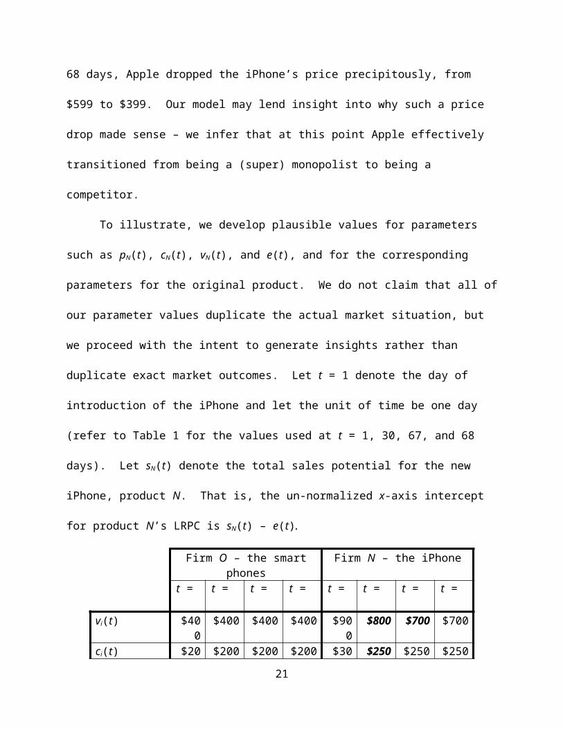
only 68 days, Apple dropped the iPhone’s price precipitously, from $599 to $399. Our model
may lend insight into why such a price drop made sense – we infer that at this point Apple
3 These might be categorized as “radically new” (Chandy and Tellis 1998) or “new to the world” (Markides 2006) products.
4 For example, a price drop may result from cost reduction resulting from learning effects (see e.g., Yelle 2007).
13
effectively transitioned from being a (super) monopolist to being a competitor.
To illustrate, we develop plausible values for parameters such as pN(t), cN(t), vN(t), and
e(t), and for the corresponding parameters for the original product. We do not claim that all of
our parameter values duplicate the actual market situation, but we proceed with the intent to
generate insights rather than duplicate exact market outcomes. Let t = 1 denote the day of
introduction of the iPhone and let the unit of time be one day (refer to Table 1 for the values used
at t = 1, 30, 67, and 68 days). Let sN(t) denote the total sales potential for the new iPhone,
product N. That is, the un-normalized x-axis intercept for product N’s LRPC is sN(t) – e(t).
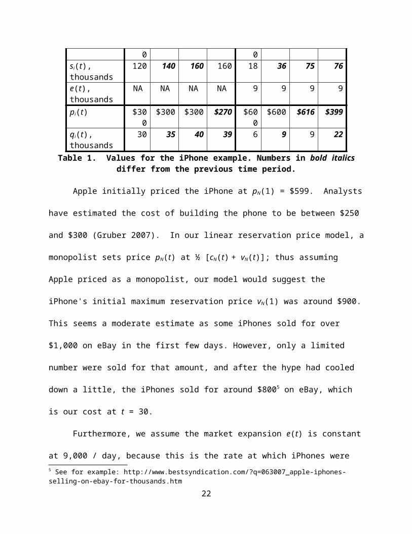
Firm O – the smart phones Firm N – the iPhonet = 1 t = 30 t = 67 t = 68 t = 1 t = 30 t = 67 t = 68
vi(t) $400 $400 $400 $400 $900 $800 $700 $700ci(t) $200 $200 $200 $200 $300 $250 $250 $250si(t), thousands 120 140 160 160 18 36 75 76e(t), thousands NA NA NA NA 9 9 9 9pi(t) $300 $300 $300 $270 $600 $600 $616 $399qi(t), thousands 30 35 40 39 6 9 9 22
Table 1. Values for the iPhone example. Numbers in bold italics differ from the previous time period.
Apple initially priced the iPhone at pN(1) = $599. Analysts have estimated the cost of
building the phone to be between $250 and $300 (Gruber 2007). In our linear reservation price
model, a monopolist sets price pN(t) at ½ [cN(t) + vN(t)]; thus assuming Apple priced as a
monopolist, our model would suggest the iPhone's initial maximum reservation price vN(1) was
around $900. This seems a moderate estimate as some iPhones sold for over $1,000 on eBay in
the first few days. However, only a limited number were sold for that amount, and after the hype
had cooled down a little, the iPhones sold for around $8005 on eBay, which is our cost at t = 30.
Furthermore, we assume the market expansion e(t) is constant at 9,000 / day, because this
is the rate at which iPhones were selling on day 67 (Crum 2007; Elmer-DeWitt 2007), just prior
5 See for example: http://www.bestsyndication.com/?q=063007_apple-iphones-selling-on-ebay-for-thousands.htm
14
to Apple’s transition from being a monopolist to being a competitor (in our model this transition
occurs only after saturation of the new market). We assume somewhat arbitrarily that sN(1) =
18,000 / day, suggesting that some of the highest-end original customers also considered the
iPhone upon its introduction, although not enough to actually purchase it at the $599 price tag.
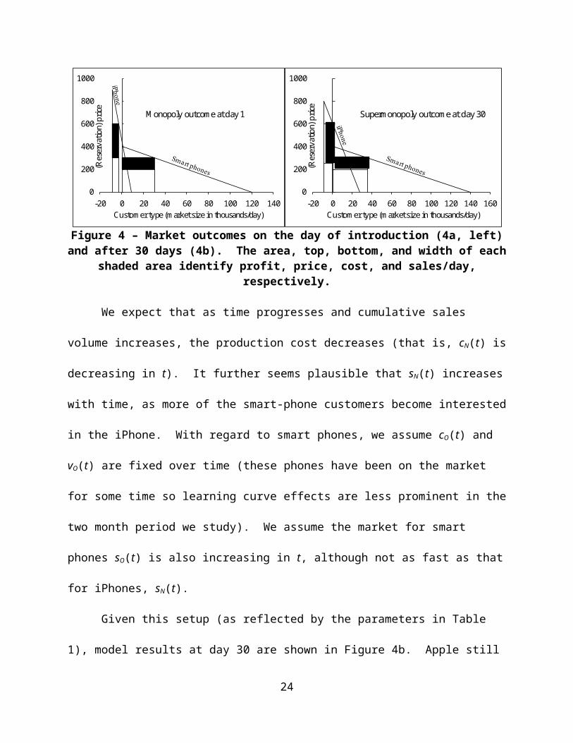
Smart-phones were priced at about $400 at the introduction of the iPhone, but Verizon gave a
$100 discount with the purchase of a two year service agreement (Verizon 2007). We therefore
set pO(1) = $300 and assume that cO(1) = $200 and vO(1) = $400. Smart-phones sold at a rate of
roughly 30,000 per day at t = 1(Martin 2008), and from these parameters we infer the sales
potential of sO(1) = 120,000 / day. Plugging these parameters into our LRPCM, we end up with
initial sales of 6,000 iPhones / day. See Figure 4a.
0
200
400
600
800
1000
-20 0 20 40 60 80 100 120 140
(Res
erva
tion)
pric
e
Customer type (market size in thousands/day)
Monopoly outcome at day 1
0
200
400
600
800
1000
-20 0 20 40 60 80 100 120 140 160
(Res
erva
tion)
pric
e
Customer type (market size in thousands/day)
Supermonopoly outcome at day 30
Figure 4 – Market outcomes on the day of introduction (4a, left) and after 30 days (4b). The area, top, bottom, and width of each shaded area identify profit, price, cost, and
sales/day, respectively.
We expect that as time progresses and cumulative sales volume increases, the production
cost decreases (that is, cN(t) is decreasing in t). It further seems plausible that sN(t) increases with
time, as more of the smart-phone customers become interested in the iPhone. With regard to
smart phones, we assume cO(t) and vO(t) are fixed over time (these phones have been on the
market for some time so learning curve effects are less prominent in the two month period we
15
study). We assume the market for smart phones sO(t) is also increasing in t, although not as fast
as that for iPhones, sN(t).
Given this setup (as reflected by the parameters in Table 1), model results at day 30 are
shown in Figure 4b. Apple still chooses to act as a super-monopolist, pricing at $600 (the
limited additional sales that would be realized by acting as a duopolist6 would not offset the
resulting loss in per-unit margin).
After 67 days (see Figure 5a) we assume the total potential market sizes of the iPhone
and smart phones have increased to sN(67) = 75,000/day and sO(67) = 160,000/day, and the
iPhone’s maximum reservation price has dropped to vN(67) = $700 while all other parameters
remain unchanged from day 30. Apple’s optimal super-monopoly remains around $600 and this
price generates just 1% higher profit as compared to the optimal expanded duopoly price of
about $400. In other words, conditions have almost, but not quite, reached the point at which
Apple should transition from a super-monopolist to a duopolist.
0
200
400
600
800
-20 0 20 40 60 80 100 120 140 160 180
(Res
erva
tion)
pric
e
Customer type (market size in thousands/day)
Supermonopoly outcome at day 67
0
200
400
600
800
-20 0 20 40 60 80 100 120 140 160 180
(Res
erva
tion)
pric
e
Customer type (market size in thousands/day)
Duopoly outcome at day 68
Figure 5 – Market outcomes after 67 days (5a, left) and after 68 days (5b).
Notice that from t =1 to t = 30 to t = 67 we have seen gradual increases in the market
size, sN(t) and gradual decreases in the iPhone cost, cN(t). At day 68 (see Figure 5b), we assume
6 Here we use the term “duopoly” to imply a market with the iPhone competing against other smart phones. Our analysis is not of a granularity that can distinguish between every other smart phone; it simply considers them as a single original product.
16
another slight increase in the potential market size to sN(68) = 76,000/day, up from 75,000/day,
while keeping all the other parameters fixed. This seemingly undisruptive change results in
Apple realizing approximately 0.1% higher profit in an expanded duopoly than in the super
monopoly. Thus Apple now chooses the expanded duopoly, which is associated with an optimal
iPhone price of roughly $400, representing a precipitous drop from $600 just the previous day.
As observed by Elmer-DeWitt (2007), our model suggests iPhone sales increase
dramatically as a consequence of the price drop. The optimal price for other smart phones drops
a bit from pO(67) = $300 to pO(68) = $270 in response to the iPhone’s new competitive stance
(our model suggests a firm such as Sony-Ericsson should now offer an additional $30 rebate),
while sales of other smart phones drop slightly from 40,000 to 39,000 per day.
In summary, our model suggests the iPhone initially created a new market, allowing
Apple to price like a monopolist. Customer perceptions and product costs changed over time but
the optimal price remained relatively constant through day 67. On day 68 Apple found it optimal
to transition from a (super) monopolist to competing directly with other smart-phones, by
precipitously dropping price. Of course our model is a simplification of reality and as such does
not account for many relevant factors within the smart phone segment. However, while the
numbers relevant to our example may not fully reflect reality, our model may lend insight into
why it might have been desirable for Apple to introduce such an abrupt change in price in spite
of a presumed gradual, continuous change in market parameters.
4. DISCUSSION AND SUMMARY
In addition to the iPhone example, it is interesting to briefly consider the implications of our
framework relative to the new Tesla automobile. While Christensen (1997) suggested that a
low-end (disruptive) strategy might be desirable for the electric car, Tesla has apparently decided
17
that its preferred approach is a new-market high-end strategy.7 In 2008 Tesla began production
of the Roadster which is based on the Lotus Elise chassis and, with a price tag of $98,000, can
accelerate from 0 to 60 in 4 seconds and travel up to 245 miles on one charge. There was a
waiting list for the 2008 planned production of 600 cars (White 2007). The Roadster’s
performance, price, and waiting list suggest Tesla has a high degree of pricing power and its car
is aimed at high-end consumers. Tesla’s appeal is to the environmentally conscious customer
who enjoys luxury – this gives Tesla the ability to open a new market, again suggesting new-
market high-end encroachment.
Our model would suggest that if Tesla wishes to continue to grow volume over time, it
will eventually need to make the transition into competition with existing high-performance cars,
and possibly to other more mainstream vehicles as well. This will lead to diminishing pricing
power; thus Tesla must achieve continual cost reduction so that it can continue to encroach
down-market if it strives to grow sales volume. Tesla is already planning for a $50,000 dollar
sedan in 2010, to compete directly with luxury car manufacturers like Lexus, Cadillac, and
BMW (White 2007). The real gauge of the Tesla’s success will be its ability to weather the
change to competing more aggressively against market incumbents. Tesla’s $50,000 sedan will
encroach upon the luxury car market in a high-end new-attribute pattern, but with other luxury
car makers like BMW and Lexus racing to introduce hydrogen, electric and hybrid cars, Tesla
will face some competition in the new-market space. To enhance its image as a firm marketing
new-attributes as the same time that it moves downstream in the market, Tesla might consider
continual strengthening of ancillary attributes to make the cars even more attractive, such as
partnering with Apple to provide seamless stereo equipment that synchronizes directly to iPod.
7 We do not intend to imply that either Christensen or Tesla has specified the wrong approach, as there may be multiple viable strategies. However we would suggest that prior to the development of a new high-end product, a firm should comprehensively consider all three encroachment alternatives and pick the one it deems optimal.
18
In summary, Tesla needs to continually offer higher performance along ancillary
dimensions or it faces stronger competition with existing vehicles, in which case cost
improvements will become more critical. Because Tesla can initially price quite high, it has
been given a window of opportunity in which it must develop its supply chain and streamline its
processes so that it can significantly reduce cost before competing directly with other firms.
Similar to TiVo, who licensed its technology to manufacturers with economies of scale like
Philips and Sony, a possibility would be for Tesla to consider licensing its patented battery
technology to hybrid car manufactures. This would lead to significantly higher volume of sales
for Tesla’s battery technology, and would thus lead to faster process and cost improvements.
While the Tesla example is an interesting case study, our model does not go so far as to
prescribe the optimal encroachment strategy for any given product. Rather, our intent is to
promote understanding of the various possible high-end encroachment types, and the
implications of the alternate strategies. More work is needed to delineate for a firm the
conditions under which each strategy is optimal. A paper that pursues insights of this type is
Van der Rhee et al. (2010), which discusses Nintendo’s choice of the fringe-market low-end
strategy in introducing the Wii. Given that a product may encroach on multiple markets, it also
seems apparent that a manager must have the ability to see her products in the context of
multiple markets. Tellis (2006) labels this ability to see products in relationship to other
competing innovations as visionary leadership – our framework and insights are aimed at further
improving the vision of such leaders and assist them in new product introductions.
19
APPENDIX A – DEVELOPMENT OF LRPC MODEL USING PART-WORTH CURVES
In developing the linear reservation price curve (LRPC) model, we follow the approach of Schmidt and Porteus (2000), which in turn is based on a number of standard assumptions in the literature. A customer’s part-worth for each attribute of each product is defined to be the most that she is willing to pay for the performance of that product along that attribute dimension. We assume there are two key attributes; the old product’s core attribute and a new (or ancillary) attribute that may be offered by the new product.8 Thus by definition, the performance of the old product along the new attribute dimension is weak (for simplicity, assume those part-worths are zero) and therefore a customer’s reservation price for the old product (the most she is willing to pay for the products) is simply equal to her part-worth for the old product’s core attribute. A customer’s “type” is determined by her part-worth for the old product’s core attribute, and we assume these part-worths are uniformly distributed from zero to some maximum. This means that if all customers are ordered along the x-axis according to type, from highest part-worth (willingness to pay) down to the lowest, the resulting part-worth curve can be approximated by a continuous straight line. Keeping the same ordering of customers, we similarly plot the part-worths for the new product’s core attribute, and for the new product’s new (ancillary) attribute. We assume each of these part-worth curves is also linear, and assume that a customer’s reservation price is the sum of her part-worths for the individual attributes. Since the part-worth curves are linear, their sum (i.e., the reservation price curve) will also be linear (technically, affine), and hence the term LRPC.
More formally, at some given point in time, let s denote the number of customers in the old product market and let x denote customer type such that x∈(0 , s). We assume that each attribute is vertically differentiated (e.g., Moorthy 1988), meaning that if the attribute performance is increased, it increases every customer’s part-worth (i.e., willingness to pay). We denote customer x’s part-worths for product O’s core and new attributes by vO
C – xkOC and vO
N – xkO
N, respectively, where kOC and kO
N denote O’s relative performance (or ascribed quality) along the core and new dimensions, respectively, and where vO
C and vON are the part-worths for a
customer of type zero. Similarly, at some given point in time, customer x’s part-worths for product N’s core and
new attributes are vNC – xkN
C and vNN – xkN
N, respectively. Without loss of generality we assume kO
C(t) is positive, and given that N performs better along the core dimension (it is a high-end product), we have kN
C(t)> kOC(t). The slope kO
N(t) may be either positive or negative (there may be a positive or negative correlation between the strengths of customer preferences for the core and new attributes), but |kO
N(t)| is again a measure of attribute performance or ascribed quality. By definition, the core attribute performance is of utmost importance to O’s customers so we assume k(t) ≡ kO
C(t) + kON(t) > 0. We assume that N also performs better along the new
dimension (in addition to the core dimension) so |kNN(t)| > |kO
N(t)|. If kNN(t) > kO
N(t) > 0 then clearly, kN
C(t) + kNN(t) > kO
C(t) + kON(t) which validates our assumption that N has a steeper
reservation price curve. If kNN(t) < kO
N(t) < 0 then our assumption does not hold when kNC(t) –
kOC(t) < |kN
N(t)| – |kON(t)|. However, this scenario does not seem credible – it seems superfluous
to pursue the strategy of greatly enhancing new attribute performance along with improved core attribute performance in the case where customer strengths of preference across core and new
8 If there is more than one core attribute, we assume the part-worth curve for each of these core attributes is affine, and we add up these individual part-worth curves to obtain the part-worth curve that we speak of herein as the core-attribute’s curve. We handle multiple new (i.e., ancillary) attributes similarly.
20
attributes are negatively correlated.9 In addition to the customers in the interval x∈(0 , s) we assume there is a new market of
high-end customers in the interval x∈(−e , 0). These customers have latent (dormant) part-worths for the core attribute; these part-worths are activated only in the presence of the new attribute (i.e., are only activated by the new product). For example, consider the iPhone as the new product, and consider some other smart phone as the old product. Prior to the introduction of the iPhone, buying a smart phone did not appeal to new-market customers, but the introduction of the new features that the iPhone offered lured these customers into the market. These new-market customers highly valued the core features of a conventional smart phone, in addition to highly valuing the new features that the iPhone offered. Thus for new-market customers we assume that the linear part-worth curves for the core and new attributes of the new product are linear extensions into the new market – refer to Figure 1b to see how the reservation price curve of the new product extends (leftward) into the new market. However, we assume that the part-worth curve for the core attribute of old product (and hence the reservation price curve for the old product) does not extend into the new market, because these new-market customers do not value the core attribute in the absence of the new attribute.
APPENDIX B – THE FIVE POSSIBLE MARKET OUTCOMES IN A DUOPOLY
Given the setup described in § 2.1, there are five possible market outcomes. We delineate these outcomes in Theorem 1 below, which map to the immediate, new-attribute, and new-market high-end encroachment patterns as discussed in 2.2 – 2.4. For ease of presentation we do not show the time dependencies; e.g., we abbreviate mN(t) as simply mN. We ignore the uninteresting cases where product N or O is of no consequence (gets no sales when a monopolist). Theorem 1 delineates all (five) possible outcomes, which depend on the four parameters e, k, mN ≡ (1 – cN), and mO. The possible outcomes are described in the order of least to most impact on product O; the proof is available upon request. In preparation for Theorem 1, define * ≡
, where
Y ≡ , and define
** ≡ . We denote Case 1 as the case where * ≤ ** and denote Case 2 as the case where ** ≤ *.Theorem 1. When one firm offers product N and a second firm offers product O, the market structure represents a unique Nash equilibrium outcome. Prices, quantities, and profits are as follows.
9 If the strengths of customer preferences are negatively correlated across the core and new attributes, then greatly strengthening the new attribute performance will make product N only marginally more appealing to those customers who most appreciate the improved core attribute performance (i.e., O’s high-end customers). At the same time, those customers who do greatly appreciate the very strong new attribute performance (i.e., O’s low-end customers) do not really appreciate N’s stronger core performance.
21
Market Product N Product O
Solution is optimal if .1. Dual monopolies (N and O each acts as a monopolist)
pN=1+cN+e
2 ; qN=
mN+e2 ; π N=qN
2 pO=vO+cO
2 ; qO=
mO
2k ; πO=kqO2
Solution is optimal in Case 1, where * ≤ **, if ,
and in Case 2 where ** ≤ *, if .2. Super Monopoly for N, Monopoly for O
pN=1; qN=e
; π N=emN pO=
vO+cO
2 ; qO=
mO
2k ; πO=kqO2
Solution only applies in Case 1, where * ≤ **, and is optimal if .
3. (Expanded) Differentiated Duopoly
pN=2 (1+cN )−mO−k+2 e (1−k )
4−k
qN=(2−k ) mN−mO+2e (1−k )
(1-k ) ( 4−k ) ;
pO=2 (vO+cO )−km N−kvO+ek (1−k )
4−k
qO=(2−k )mO−kmN+ek (1−k )
k (1-k ) ( 4−k ) ;πO=k (1−k ) qO
2
Solution is optimal in Case 1, where * ≤ **, if ,
and in Case 2, where ** ≤ *, if .4. Constrained Monopoly for N pN=1−
mO
k ;qN=e+
mO
kpO=cO ;
qO=0;
πO=0
Solution is optimal if .5. Monopoly for N
pN=1+cN+e
2 ; qN=
mN+e2 ;
pO≥cO ; qO=0
; πO=0
The first possibility shown in Theorem 1 is that of dual monopolies: If the cost of the new product is relatively high and the market expansion (e) is significant (specifically, if e > mN), then firm N chooses to sell only in the new market (leaving the original market to firm O). Thus, firm N prices as a monopolist selling only to some fraction of the new market (yielding sales quantity of less than e) and firm O prices as a monopolist in the original market.
The second possible outcome is that product N achieves what we refer to as a super monopoly (so named because firm N chooses to price at something greater than product N’s monopoly price) while product O is sold at its monopoly price and quantity. This occurs when mN > e. To explain this outcome, we begin by denoting N’s monopoly price by pN
M (representing the price firm N would charge if product N were the only product offered). If mN > e and firm N has a monopoly, we find pN
M < 1 and the associated sales quantity (denoted by qNM) would be
greater than e, meaning that the new product would sell to all customers in the new market plus
22
some customers in the original market. However, when its new product is in competition with firm O’s original product, firm N may find that pricing to attract some of these customers in the original market may be undesirable. In this case firm N instead chooses to price higher than the monopoly price (at pN = 1 > pN
M), thereby limiting the new product’s attractiveness (and its sales) to only the new market customers (i.e., to set sales qN equal to e).
Firm N finds it desirable to price as a super-monopolist when reducing the price below pN
= 1 would have one of two possible negative effects; either it would reduce firm N’s profit margin in the new market while failing to gain firm N any sales in the original market (we will refer to this as case 2.1, which would happen when firm N would set a price pN such that 1 – mO / 2 < pN < 1), or, it would induce competition with the original product in the original market (we will refer to this as case 2.2, which would happen when price pN < 1 – mO / 2). In case 2.1 firm N instead continues to price at pN = 1 > pN
M so as to avoid unnecessarily giving up margin. Firm N also wants to avoid case 2.2 – unless the profit it makes by competing in the original market more than offsets the profit it loses by lowering its price in the new market (if the profit in the original market more than offsets the lost margin then a differentiated duopoly results, as described below). In summary, firm N’s super-monopoly price and sales are pN = 1 and qN = e.
The third outcome we delineate is that of an expanded differentiated duopoly: this market equilibrium is the result when the new product N is sold to the entire new market e, along with some high-end original-market customers, while the original product sells to some lower-end original market customers. This is the outcome shown explicitly in Figure 1b. The term expanded differentiated duopoly applies if e > 0, while if e = 0 then there is no market expansion and it is simply referred to as a differentiated duopoly (this special case, where e = 0, is described in Schmidt and Porteus 2000). As Theorem 1 (case 2) shows, this outcome is not observed under some parameter values.
In the fourth possible outcome, a constrained monopoly, the new product covers the entire new market and is the only product that realizes sales in the original market. But even though firm O realizes no sales, it still constrains firm N to charge less than its monopoly price (if firm N charged its monopoly price, firm O would gain some sales, therefore firm N finds it optimal to prevent this by charging less than its monopoly price). Note that in this scenario, firm O prices at cost and firm N prices such that the customer who has zero surplus for the original product also has zero surplus for the new product.
In the fifth outcome, product N’s performance and cost are sufficiently attractive to the original market such that N’s monopoly price falls below O’s cost. Even though O prices at cost, O gets no sales and N has a monopoly in both the new and original markets.
We now consider the point in time where the new product is introduced. The five outcomes identified above can be reduced to three possible scenarios, summarized as follows. Thus our three high-end encroachment scenarios are comprehensive in covering all possible scenarios that stem from our model, and Van Orden et al. (2010) provide further empirical corroboration that these three scenarios are comprehensive.
First, there is the possibility that each product sells “in its own market” (the case of dual monopolies or the super monopoly/monopoly). This is “new-market high-end encroachment” – the new product (initially, at least) sells in its own new market (possibly encroachment over time into the old market is discussed below in § 2.5). Second, there is the scenario where the new product expands the market (e > 0) but competes with the old product in the old market (the case of the expanded differentiated duopoly, or constrained monopoly for N, or monopoly for N). We call this “new-attribute high-end encroachment” – the expansion of the market is due to the new
23
product’s inclusion of some new attribute that attracts new high-end customers. The third possible scenario is that the market does not expand (e = 0). In this case the new product immediately encroaches on (takes market share from) the old (in a differentiated duopoly or the constrained monopoly or monopoly); we call this “immediate high-end encroachment.”REFERENCES
Chandy, R. K., & Tellis, G. J. (1998), "Organizing for Radical Product Innovation: The
Overlooked Role of Willingness to Cannibalize," Journal of Marketing Research, 35(4), 474-
487.
Christensen, Clayton M. (1997). Innovator's Dilemma: When New Technologies Cause Great
Firms to Fail. Harvard Business School Press.
Druehl, C. T. and Schmidt, G. M. (2008). A Strategy for Opening a New Market and
Encroaching on the Lower End of the Existing Market. Production & Operations
Management, 17(1).
Markides, Constantinos (2006), "Disruptive Innovation: In Need of Better Theory," Journal of
Product Innovation Management, 23 (1), 19-25.
Moorthy, K. S. (1988). Product and Price Competition in a Duopoly. Marketing Science, 7 (2),
141-68.
Norton, John A. and Bass, Frank M. (1987). A Diffusion Theory Model of Adoption and
Substitution of Successive Generations of High-Technology Products. Management Science,
33, 1069-1086.
Rogers, Everett M. (1995), “New Product Adoption and Diffusion,” Journal of Consumer
Research, 2 (4), 290–302.
Schmidt, G. M., “Low-end and High-end Encroachment Strategies for New Products.” 2004.
International Journal of Innovation Management. Vol. 8, No. 2.
Schmidt, G. M. and C. T. Druehl (2005). “Changes in Product Attributes and Costs as Drivers of
New Product Diffusion and Substitution.”. Production & Operations Management, 14(3).
Schmidt, G. M. and Druehl C. T. (2008). When is a Disruptive Innovation Disruptive? Journal of
Product Innovation Management, 25 (4).
Schmidt, G. M. and Porteus E. L. (2000). The Impact of an Integrated Marketing and
Manufacturing Innovation. Manufacturing & Service Operations Management, 2(4), 317.
Tellis, G. J. (2006). Disruptive Technology or Visionary Leadership? Journal of Product
Innovation Management, 23 (1), 34-38.
24
Van der Rhee, B., G. M. Schmidt, and W. Tsai (2010). Sustain or Disrupt? Working Paper,
Nyenrode Business Universiteit.
VanOrden, J., Van der Rhee, B., and Schmidt, G.M. (2010). Encroachment Patterns of the Best
Products from the Past Decade. Forthcoming, Journal of Product Innovation Management.
White, Joseph B. (2007). Electric Car Maker Aims For the Top With Sports Car. Wall Street
Journal. New York City.
Yelle, Louis E. (2007). The Learning curve: Historical Review and Comprehensive Survey.
Decision Sciences, Volume 10 (2), 302 – 328.
25