AN OVERVIEW OF

MORPHOLOGICAL FILTERING

Jean Serra & Luc Vincent1

Centre de Morphologie Math�ematique�Ecole Nationale Sup�erieure des Mines de Paris

35, rue Saint-Honor�e

77305 Fontainebleau CedexFRANCE

Published in Circuits, Systems and Signal Processing,

Vol. 11, No. 1, pp. 47{108, January 1992

1Presently: Harvard University, Division of Applied Sciences, Pierce Hall, 29 Oxford Street, Cambridge MA 02138,

U.S.A.

Abstract

This paper consists in a tutorial overview of morphological �ltering, a theory introduced in 1988 in thecontext of mathematical morphology. Its �rst section is devoted to the presentation of the lattice framework.The emphasis is put on the lattices of numerical functions in digital and continuous spaces. The basic �lters,namely the openings and the closings, are then described and their various versions are listed. In the thirdsection, morphological �lters are de�ned as increasing idempotent operators, and their laws of compositionare proved. The last sections are concerned with two special classes of �lters and their derivations: �rst, thealternating sequential �lters allow one to bring into play families of operators depending on a positive scaleparameter. Finally, the center and the toggle mappings modify the function under study by comparing it,at each point, with a few reference transforms.

1 Mathematical morphology for complete lattices

1.1 Introduction

We de�ne a morphological �lter as an operator , acting on a complete lattice T [4], which:

(i) preserves the ordering � of T , i.e.,

X � Y =) (X) � (Y ); X; Y 2 T

(ii) is idempotent, i.e., ( (X)) = (X); X 2 T :

The �rst condition, which is called growth or increasingness, just means that, since we deal with lattices,we decide to focus on the transformations which preserve one of the basic lattice features (just as, invector spaces, one pays attention to the operators which commute with addition and scalar product, e.g.,convolutions). The second condition responds to the fact that an increasing operation is non reversible andlooses information. Idempotence stops such a simplifying action at its �rst stage.

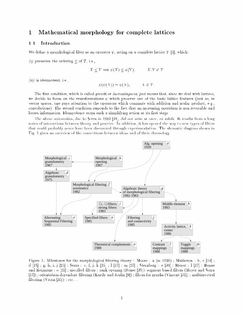
The above axiomatics, due to Serra in 1982 [24], did not arise at once, ex nihilo. It results from a longseries of interactions between theory and practice. In addition, it has opened the way to new types of �ltersthat could probably never have been discovered through experimentation. The shematic diagram shown inFig. 1 gives an overview of the connections between ideas and of their chronology.

Alg. opening1920

Morphologicalopening1967

Morphologicalgranulometry1967

Algebraicgranulometry1975

Morphological filteringaxiomatics1982

AlternatingSequential Filtering1985

Algebraic theoryof morphological filtering1982-1983

Middle element1983

-, -filters,strong filters1983

Specified filters1985

Theoretical complements1988

Contrastmappings1988

Togglemappings1988

Activity lattice,center1986

Filteringand connectivity1985

c b

a

gf

i

ne j

h

k

mlo

d

∨ ∧

Figure 1: Milestones for the morphological �ltering theory : Moore : a (� 1920) ; Matheron : b, c [14] ;d [15] ; g, h, i, j [25] ; Serra : e, f, j, k [25] ; l [17] ; m [27] ; Sternberg : e [30] ; Meyer : l [17] ; Ronseand Heijmans : o [21] ; speci�ed �lters : rank opening (Ronse [20]), segment based �lters (Meyer and Serra[17]) ; orientation dependent �ltering (Kurdy and Jeulin [9]) ; �lters for graphs (Vincent [31]) ; multispectral�ltering (Vitria [35]) ; etc: : :

1

During the late seventies, practitioners generalized in two ways the concept of a morphological opening(or closing), initially designed for sets. Firstly, they applied it to functions (Meyer, Sternberg) and to planargraphs (Lantu�ejoul). Secondly, they started composing closings with openings. The �rst extension led tobase the theory on complete lattices, whereas the second one is at the origin of the morphological �lteringaxiomatics, proposed in 1982. The same year and one year later, Matheron established a series of majortheoretical results : lattice of the �lters, _- and ^-�lters, strong �lters, middle element, the four envelopes: : : ,and extended these results to increasing (but not necessarily idempotent) operators. The part of Matheron'stheory which is presented in this overview corresponds to x 3.

Matheron's concept of middle element suggested to Serra in 1986 the ideas of morphologiocal center andactivity lattice [25, chapter 8]. A further step led the same author to leave increasingness and to introducethe notion of toggle operations [27]. This approach allows in particular to associate optimization criteria tomorphological transformations. It is presented below in x 5.

Several other pieces of theory exist, that we shall not develop here. We may quote, among others,the relationships between �ltering and connectivity preservation (Matheron and Serra, [25, chapter 7]), aninstructive approach to multispectral �ltering due to Vitria [35] and the properties of sequential monotoneconvergence established by Heijmans and Serra [7]. The pedagogical purpose of this document imposes tokeep down such derivations and to prune the text of many technicalities. For the same reason, a speciale�ort has been put on �gures and on practical comments.

1.2 Algebraic framework of the complete lattices

Inclusion is a set oriented notion. The scenes under study may be modeled by sets, but also by grey-tonefunctions, by multi-spectral functions, by graphs, each of them acting either on the Euclidean space IRn oron digital ones, like ZZn. All these situations share a common denominator formed by the two ideas whichde�ne the notion of a complete lattice T [4], namely:

1. there exists a partial ordering � over T ,2. for any (�nite or in�nite) family (Ai) in T , there exists:

� a smallest majorant _Ai called the \sup" (for supremum),

� a largest minorant ^Ai called the \inf" (for in�mum).

In particular, T posesses a greatest element, E, and a smallest one, ;. In a lattice, any logical consequenceof a choice of ordering remains true when we commute the symbols _ and ^, and � and �. This is calledthe principle of duality with respect to the order.

Here is now a review of a few basic lattices:

1.2.1 Boolean lattices

Start from an arbitrary set E. Obviously, the set P(E) of the subsets of E, which is ordered for the inclusionrelationship, is a complete lattice for the operations [ (union) and \ (intersection). Moreover, with eachX 2 P(E), there exists a unique XC 2 P(E), called the complement of X, such that:

X \XC = ; and X [XC = E: (1)

Finally, P(E) also satis�es the important property of general distributivity under which, for all Y 2P(E) and any family (Xi) of elements of P(E), we have:

([Xi) \ Y =

[(Xi \ Y ); (2)

(\Xi) [ Y =

\(Xi [ Y ): (3)

2

1.2.2 Topological lattices

When E is a topological space, its open sets generate a complete lattice for the inclusion, where the supcoincides with the union and where inf(Xi) is the interior of

TXi. This lattice is not complemented. It

satis�es the general distributivity of the type (2), but �nite distributivity only of the type (3). Indeed, inthe general case of an in�nite family (Xi), we have

([Xi) \ Y =

[(Xi \ Y ); (4)

but only

�z }| {(\Xi)[Y =

�z }| {\(Xi [ Y ) : (5)

Similar structures are derived for the closed sets and the compact sets.

1.2.3 The convex lattice

The class of the convex sets of the Euclidean space IRn generates a complete lattice where the inf coincideswith intersection and where the sup is the convex hull.

1.2.4 The partition lattice

In the set of the partitions of an arbitrary set E, we can introduce the following ordering: a partition A issmaller than a partition B when each class of A is included in a class of B. This leads to a lattice which iscomplete, but neither complemented nor distributive.

1.2.5 Function lattices

Let E be an arbitrary space. The class F of the \extended" real valued functions f : E �! IR is obviouslyordered by the relation: f � g if for each x 2 E, f(x) � g(x) and constitutes a complete lattice. The supand the inf are given by the relationships:

f = _fi () f(x) = sup fi(x); 8x 2 E;f 0 = ^fi () f 0(x) = inf fi(x); 8x 2 E: (6)

The lattice is completely distributive but not complemented. Rel. (6) implies that f(x) may equal +1.However, if we want to restrict ourselves to bounded functions, it su�ces to remark that the previous latticeis isomorphic (by anamorphosis) to

� either the class F 0 of the non negative functions f : E �! [0;+1],

� or the class F 00 of the functions f : E �! [0; 1].

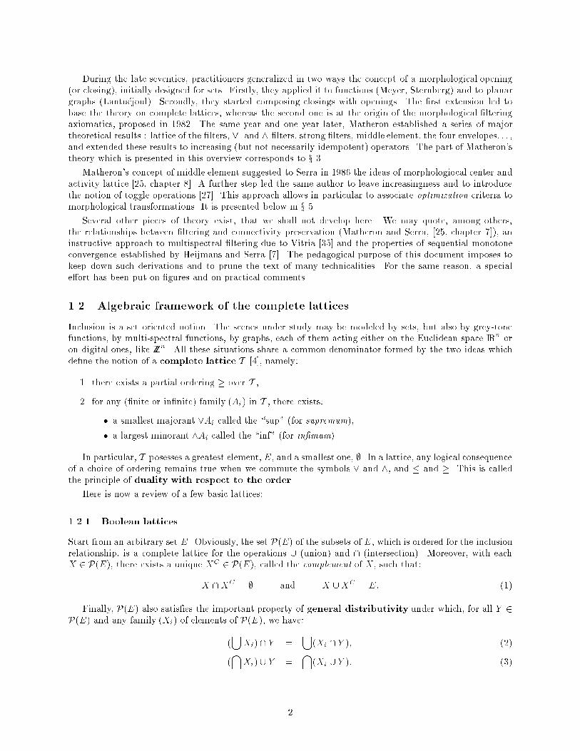
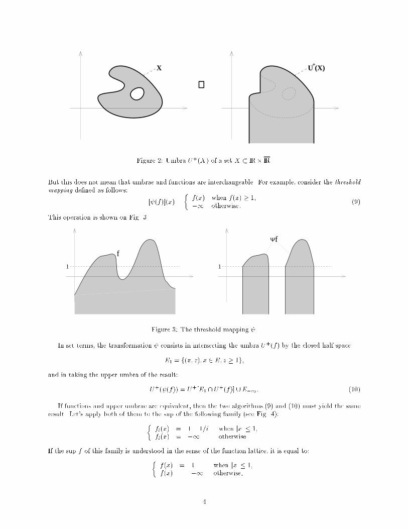
Functions and umbrae: Is it possible to identify the function lattice F with the set class of the associatedsubgraphs, or umbrae? Remember that with every function f : E �! IR (and more generally with every setin E � IR, see Fig. 2), we can associate the two sets U+(f) and U�(f) of E � IR de�ned by the relations:

U+(f) = f(x; z) 2 E � IR; f(x) � zg; (7)

U�(f) = f(x; z) 2 E � IR; f(x) < zg: (8)

Clearly, every umbra comprised between U+(f) and U�(f) generates the same function f . Moreover,the associated ordering relations are equivalent, since

f � g () U+(f) � U+(g) () U�(f) � U�(g):

3

X U (X)+

⇒

Figure 2: Umbra U+(X) of a set X � IR� IR.

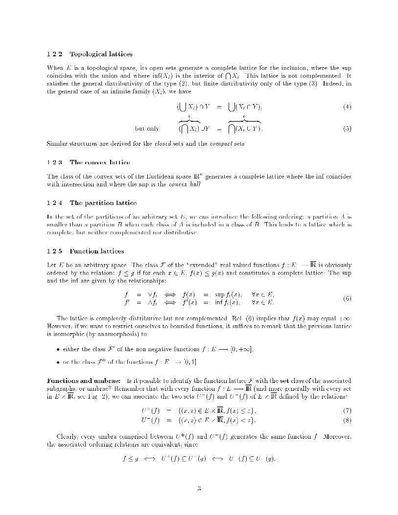
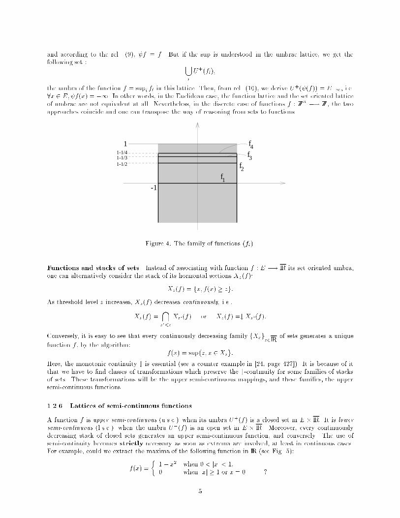
But this does not mean that umbrae and functions are interchangeable. For example, consider the thresholdmapping de�ned as follows:

[ (f)](x) =

�f(x) when f(x) � 1;�1 otherwise:

(9)

This operation is shown on Fig. 3.

f

1 1

Ψf

Figure 3: The threshold mapping .

In set terms, the transformation consists in intersecting the umbra U+(f) by the closed half space

E1 = f(x; z); x 2 E; z � 1g;

and in taking the upper umbra of the result:

U+( (f)) = U+[E1 \ U+(f)] [E�1: (10)

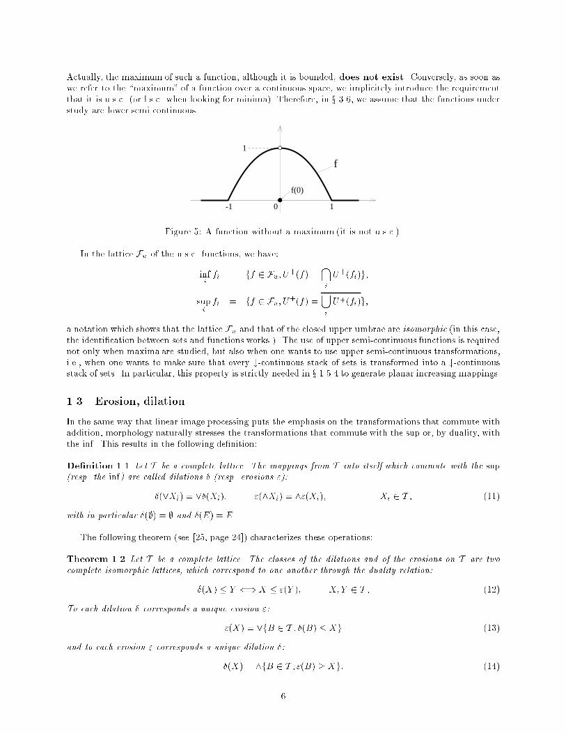
If functions and upper umbrae are equivalent, then the two algorithms (9) and (10) must yield the sameresult. Let's apply both of them to the sup of the following family (see Fig. 4):�

fi(x) = 1� 1=i when jxj � 1;fi(x) = �1 otherwise.

If the sup f of this family is understood in the sense of the function lattice, it is equal to:�f(x) = 1 when jxj � 1;f(x) = �1 otherwise,

4

and according to the rel. (9), f = f . But if the sup is understood in the umbrae lattice, we get thefollowing set : [

i

U+(fi);

the umbra of the function f = supi fi in this lattice. Then, from rel. (10), we derive U+( (f)) = E�1, i.e.8x 2 E; f(x) = �1. In other words, in the Euclidean case, the function lattice and the set oriented latticeof umbrae are not equivalent at all. Nevertheless, in the discrete case of functions f : ZZn �! ZZ, the twoapproaches coincide and one can transpose the way of reasoning from sets to functions.

f1

1-1/21-1/31-1/4

1-1

3

f1

f2

f4

Figure 4: The family of functions (fi).

Functions and stacks of sets Instead of associating with function f : E �! IR its set oriented umbra,one can alternatively consider the stack of its horizontal sections Xz(f):

Xz(f) = fx; f(x) � zg:As threshold level z increases, Xz(f) decreases continuously, i.e.,

Xz(f) =\z0<z

Xz0(f) or Xz(f) =# Xz0 (f):

Conversely, it is easy to see that every continuously decreasing family fXzgz2IR

of sets generates a unique

function f , by the algorithm:f(x) = supfz; x 2 Xzg:

Here, the monotonic continuity # is essential (see a counter example in [24, page 427]). It is because of itthat we have to �nd classes of transformations which preserve the #-continuity for some families of stacksof sets. These transformations will be the upper semi-continuous mappings, and these families, the uppersemi-continuous functions.

1.2.6 Lattices of semi-continuous functions

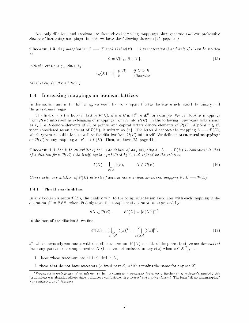
A function f is upper semi-continuous (u.s.c.) when its umbra U+(f) is a closed set in E � IR. It is lowersemi-continuous (l.s.c.) when the umbra U�(f) is an open set in E � IR. Moreover, every continuouslydecreasing stack of closed sets generates an upper semi-continuous function, and conversely. The use ofsemi-continuity becomes strictly necessary as soon as extrema are involved, at least in continuous cases.For example, could we extract the maxima of the following function in IR (see Fig. 5):

f(x) =

�1� x2 when 0 < jxj < 1;0 when jxj � 1 or x = 0 ?

5

Actually, the maximum of such a function, although it is bounded, does not exist. Conversely, as soon aswe refer to the \maximum" of a function over a continuous space, we implicitely introduce the requirementthat it is u.s.c. (or l.s.c. when looking for minima). Therefore, in x 3.6, we assume that the functions understudy are lower semi continuous.

1

f

1-1 0

f(0)

Figure 5: A function without a maximum (it is not u.s.c.).

In the lattice Fu of the u.s.c. functions, we have:

infifi = ff 2 Fu; U+(f) =

\i

U+(fi)g;

supi

fi = ff 2 Fu; U+(f) =[i

U+(fi)g;

a notation which shows that the lattice Fu and that of the closed upper umbrae are isomorphic (in this case,the identi�cation between sets and functions works.). The use of upper semi-continuous functions is requirednot only when maxima are studied, but also when one wants to use upper semi-continuous transformations,i.e., when one wants to make sure that every #-continuous stack of sets is transformed into a #-continuousstack of sets. In particular, this property is strictly needed in x 1.5.4 to generate planar increasing mappings.

1.3 Erosion, dilation

In the same way that linear image processing puts the emphasis on the transformations that commute withaddition, morphology naturally stresses the transformations that commute with the sup or, by duality, withthe inf. This results in the following de�nition:

De�nition 1.1 Let T be a complete lattice. The mappings from T into itself which commute with the sup(resp. the inf) are called dilations � (resp. erosions "):

�(_Xi) = _�(Xi); "(^Xi) = ^"(Xi); Xi 2 T ; (11)

with in particular �(;) = ; and �(E) = E.

The following theorem (see [25, page 24]) characterizes these operations:

Theorem 1.2 Let T be a complete lattice. The classes of the dilations and of the erosions on T are twocomplete isomorphic lattices, which correspond to one another through the duality relation:

�(X) � Y ()X � "(Y ); X; Y 2 T ; (12)

To each dilation � corresponds a unique erosion ":

"(X) = _fB 2 T ; �(B) � Xg (13)

and to each erosion " corresponds a unique dilation �:

�(X) = ^fB 2 T ; "(B) � Xg: (14)

6

Not only dilations and erosions are themselves increasing mappings, they generate two comprehensiveclasses of increasing mappings. Indeed, we have the following theorem [25, page 20]:

Theorem 1.3 Any mapping : T �! T such that (E) = E is increasing if and only if it can be writtenas

= _f"B; B 2 T g; (15)

with the erosions "Bgiven by

"B(X) =

� (B) if X � B,; otherwise.

(dual result for the dilation.)

1.4 Increasing mappings on boolean lattices

In this section and in the following, we would like to compare the two lattices which model the binary andthe grey-tone images.

The �rst one is the boolean lattice P(E), where E is IRn or ZZn for example. We can look at mappingsfrom P(E) into itself as extensions of mappings from E into P(E). In the following, lower-case letters suchas x, y, a, b denote elements of E, or points, and capital letters denote elements of P(E). A point x 2 E,when considered as an element of P(E), is written as fxg. The letter � denotes the mapping E �! P(E),which generates a dilation, as well as the dilation from P(E) into itself. We de�ne a structural mapping1

on P(E) as any mapping � : E �! P(E). Then, we have [25, page 41]:

Theorem 1.4 Let E be an arbitrary set. The datum of any mapping � : E �! P(E) is equivalent to thatof a dilation from P(E) into itself, again symbolized by �, and de�ned by the relation

�(X) =[x2X

�(x); X 2 P(E): (16)

Conversely, any dilation of P(E) into itself determines a unique structural mapping � : E �! P(E).

1.4.1 The three dualities

In any boolean algebra P(E), the duality w.r. to the complementation associates with each mapping theoperation � = � �, where � designates the complement operator, as expressed by

8X 2 P(E); �(X) = [ (XC )]C:

In the case of the dilation �, we �nd

��(X) = [[

x2XC

�(x)]C =\

x2XC

[�(x)]C: (17)

��, which obviously commutes with the inf, is an erosion. ��(X) consists of the points that are not descendantfrom any point in the complement of X (that are not included in any �(x) when x 2 XC ), i.e:

1. those whose ancestors are all included in X,

2. those that do not have ancestors (a �xed part S, which remains the same for any set X).

1Structural mappings are often referred to in literature as structuring functions ; further to a reviewer's remark, this

terminologywas abandonedhere since it induces a confusionwith grey-level structuring element. The term \structuralmapping"

was suggested by P. Maragos.

7

We form another duality notion by operating on the structural mapping with the transposition � 7�! ��,i.e:

��(x) = fy 2 E; x 2 �(y)g:The transpose ��(x) of �(x) is made of the set of points from which x descends, hence ��� = �. The structuralmapping �� generates the dilation ��:

��(X) = fy 2 E; �(y) \X 6= ;g: (18)

From the two relations (17) and (18), we derive the links between these two dualities, and the basic one,namely � $ " (see rel. (12)):

" = (��)� �" = �� "� = ��: (19)

1.4.2 Translation invariance

We now assume that E is equipped with a translation (e.g. E = ZZn or E = IRn), and that the dilation � is

translation invariant, i.e. is a t-dilation. In other words, the structural mapping �(h) at point h is deducedfrom that of the origin o (denoted �(o) = B) by translation: �(h) = Bh = fB + h; b 2 Bg. The set B iscalled structuring element. We see from relation (16) that

�(X) = X � B = B �X

=[x2X

Bx

= fb+ x; x 2 X; b 2 Bg=

[b2B

Xb: (20)

The t-dilation � is classically known as Minkowski addition between sets X and B. By duality undercomplementation, it gives

��(X) = �"(X) =\b2B

Xb = X B (21)

and by lattice duality:

"(X) =\b2 �B

Xb = X �B; with �B = f�b; b 2 Bg: (22)

Both operations are Minkowski subtractions of X by B and �B respectively. According to a classical resultdue to G. Matheron, any increasing t-mapping is a union of t-erosions, and also an intersection of t-dilations[15, page 221]. More precisely,

Theorem 1.5 Let be a translation invariant increasing mapping. Then, for any X 2 P(E),

(X) =[fX �B;B 2 P(E); o 2 (B)g =

\fX � �B;B 2 P(E); o 2 �(B)g:

1.4.3 Examples

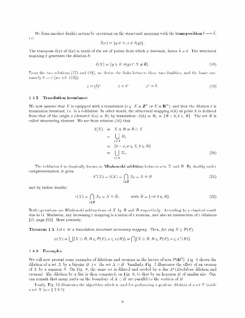
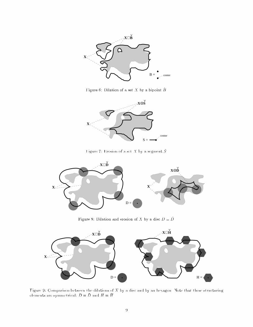
We will now present some examples of dilations and erosions in the lattice of sets P(IR2). Fig. 6 shows thedilation of a set X by a bipoint B, i.e. the set X � �B. Similarly, Fig. 7 illustrates the e�ect of an erosionof X by a segment S. On Fig. 8, the same set is dilated and eroded by a disc D (Euclidean dilation anderosion). The dilation by a disc is then compared, on Fig. 9, to that by an hexagon H of similar size. Onecan remark that many parts on the boundary of X � �H are parallel to the vertices of H.

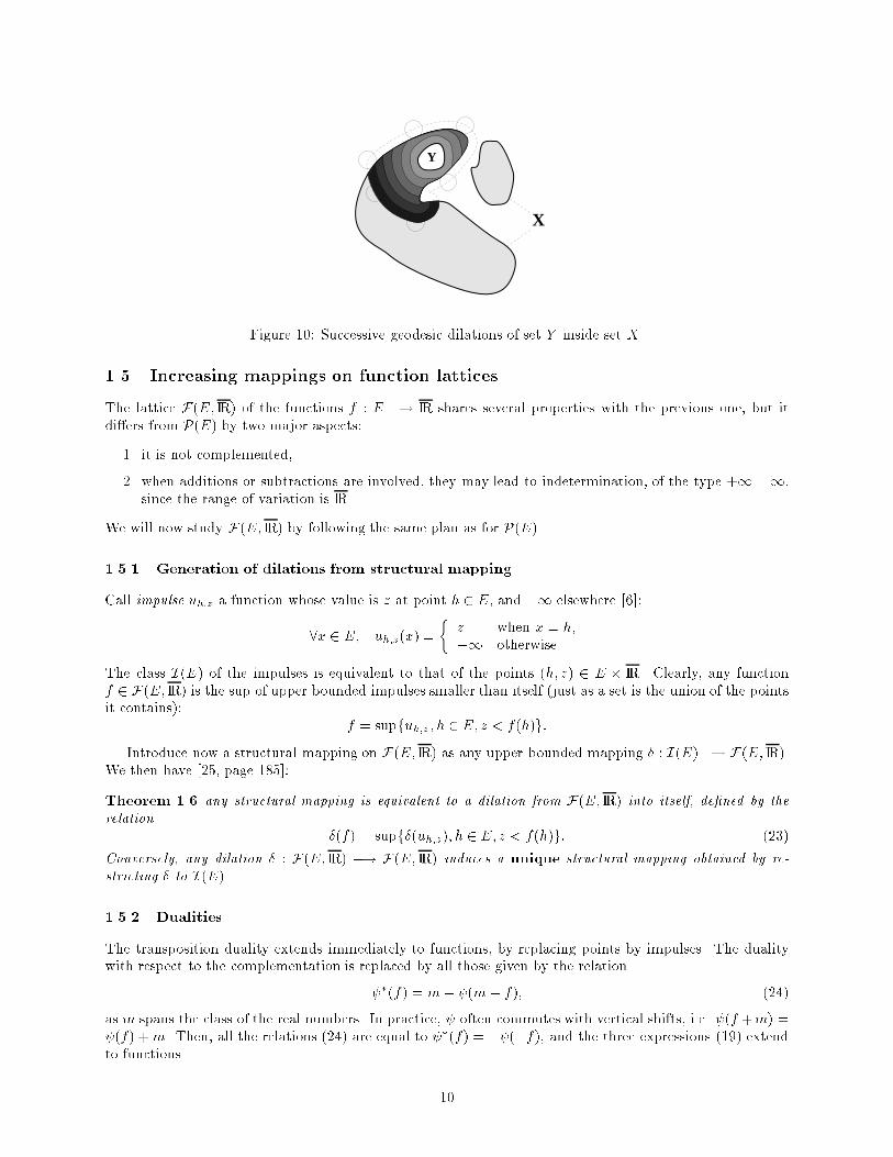
Lastly, Fig. 10 illustrates the algorithm which is used for performing a geodesic dilation of a set Y insidea set X (see x 2.4.1).

8

X

B =

X B^

center

Figure 6: Dilation of a set X by a bipoint �B.

X

S =

X SΘ^

center

Figure 7: Erosion of a set X by a segment �S.

X X

D =

X D⊕^

X DΘ^

Figure 8: Dilation and erosion of X by a disc D = �D.

X

D =

X D⊕^

H =

X H⊕^

Figure 9: Comparison between the dilations of X by a disc and by an hexagon. Note that these structuringelements are symmetrical: D = �D and H = �H.

9

X

Y

Figure 10: Successive geodesic dilations of set Y inside set X.

1.5 Increasing mappings on function lattices

The lattice F(E; IR) of the functions f : E �! IR shares several properties with the previous one, but itdi�ers from P(E) by two major aspects:

1. it is not complemented,

2. when additions or subtractions are involved, they may lead to indetermination, of the type +1�1,since the range of variation is IR.

We will now study F(E; IR) by following the same plan as for P(E).

1.5.1 Generation of dilations from structural mapping

Call impulse uh;z a function whose value is z at point h 2 E, and �1 elsewhere [6]:

8x 2 E; uh;z(x) =

�z when x = h;�1 otherwise.

The class I(E) of the impulses is equivalent to that of the points (h; z) 2 E � IR. Clearly, any functionf 2 F(E; IR) is the sup of upper bounded impulses smaller than itself (just as a set is the union of the pointsit contains):

f = supfuh;z; h 2 E; z < f(h)g:Introduce now a structural mapping on F(E; IR) as any upper bounded mapping � : I(E) �! F(E; IR).

We then have [25, page 185]:

Theorem 1.6 any structural mapping is equivalent to a dilation from F(E; IR) into itself, de�ned by therelation

�(f) = supf�(uh;z); h 2 E; z < f(h)g: (23)

Conversely, any dilation � : F(E; IR) �! F(E; IR) induces a unique structural mapping obtained by re-stricting � to I(E).

1.5.2 Dualities

The transposition duality extends immediately to functions, by replacing points by impulses. The dualitywith respect to the complementation is replaced by all those given by the relation

�(f) = m � (m � f); (24)

as m spans the class of the real numbers. In practice, often commutes with vertical shifts, i.e. (f +m) = (f) +m. Then, all the relations (24) are equal to �(f) = � (�f), and the three expressions (19) extendto functions.

10

1.5.3 Translation invariances

We can consider either a translation operation t0h, by vector h 2 E, or a translation operation th;z by avector (h; z) 2 E � IR. The two corresponding formulas are:

(th;zf)(x) = f(x � h) + z;

(t0hf)(x) = f(x � h):

We shall focus on the t-invariant mappings, which are the most useful in practice. Saying that dilation� is invariant with respect to translations is equivalent to saying that the structural mapping � is the sameeverywhere, i.e. if g = �u0;0 is the transform of the origin-impulse u0;0, then 8x 2 E; �uh;z(x) = g(x�h)+z.Then, the expression (23) of the dilation � takes the following simpler form:

(�f)(x) = supfg(x� h) + z; z < f(h); h 2 Eg; f 2 F(E; IR):

Note that the operand g(x � h) + z cannot take the undetermined form +1�1 since, for all h, x and z,each of the two numbers g(x � h) and z is < +1. Hence, we have �nally

(�f)(x) = supfg(x� h) + f(h); h 2 Eg; f 2 F(E; IR): (25)

The two dual erosions " and �" of � are given by the following formulae:

("f)(x) = inffg(x+ h)� f(h); h 2 Eg; (26)

(�"f)(x) = inffg(x� h)� f(h); h 2 Eg:

Similarly to theorem 1.5, any increasing mapping : E �! IR which is t-invariant may be decomposedinto a sup of erosions as well as into an inf of dilations (same proof as for theorem 1.5).

1.5.4 Planar increasing mappings

Generally speaking, the representation of a function f : E �! IR by the stack of its sections allows one togenerate a function transformation on f from every set transformation : E �! E. It su�ces to put

Xz( (f)) =\z0<z

[Xz0 (f)]:

Then, one speaks of planar transformation, or again of stack transformation. Obviously, the familyXz( (f))is continuously decreasing with z. Hence, it generates a function. This technique has been used for examplein [24, page 451] to derive the thickening for functions from that for sets.

However, it is for increasing mappings that the planar increasing transformations have been the moreextensively studied. A basic reference is here Serra [24, pages 426{434]. One can refer as well to [25, chapter9] or to Maragos and Schafer [13]. See also Sternberg [30], Meyer [16], Rosenfeld [22] and Yli-Harja, Astolaand Neuvo [37]. Here, in the continuous case, we have to assume that is upper semi-continuous, whichimplies that it preserves the #-continuity, i.e.,

[Xz(f)] =\z0<z

[Xz0 (f)]:

Then, the de�nition of the planar mapping leads to:

Xz [ (f)] = [Xz(f)]: (27)

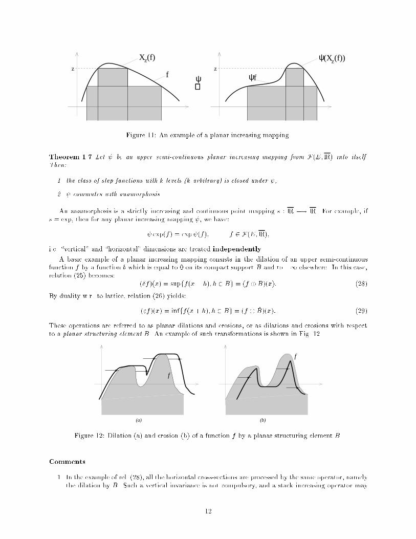
This relation is illustrated by Fig. 11.

In other words, the planarity of the mapping allows us to process f threshold by threshold. A seriesof results derive directly from the key relation (27), namely:

11

z z

fψ⇒

f

X (f)z

ψ

(X (f))zψ

Figure 11: An example of a planar increasing mapping.

Theorem 1.7 Let be an upper semi-continuous planar increasing mapping from F(E; IR) into itself.Then:

1. the class of step functions with k levels (k arbitrary) is closed under ,

2. commutes with anamorphosis.

An anamorphosis is a strictly increasing and continuous point mapping s : IR �! IR. For example, ifs = exp, then for any planar increasing mapping , we have:

exp(f) = exp (f); f 2 F(E; IR);

i.e. \vertical" and \horizontal" dimensions are treated independently.

A basic example of a planar increasing mapping consists in the dilation of an upper semi-continuousfunction f by a function b which is equal to 0 on its compact support B and to �1 elsewhere. In this case,relation (25) becomes:

(�f)(x) = supff(x� h); h 2 Bg = (f �B)(x): (28)

By duality w.r. to lattice, relation (26) yields:

("f)(x) = infff(x + h); h 2 Bg = (f �B)(x): (29)

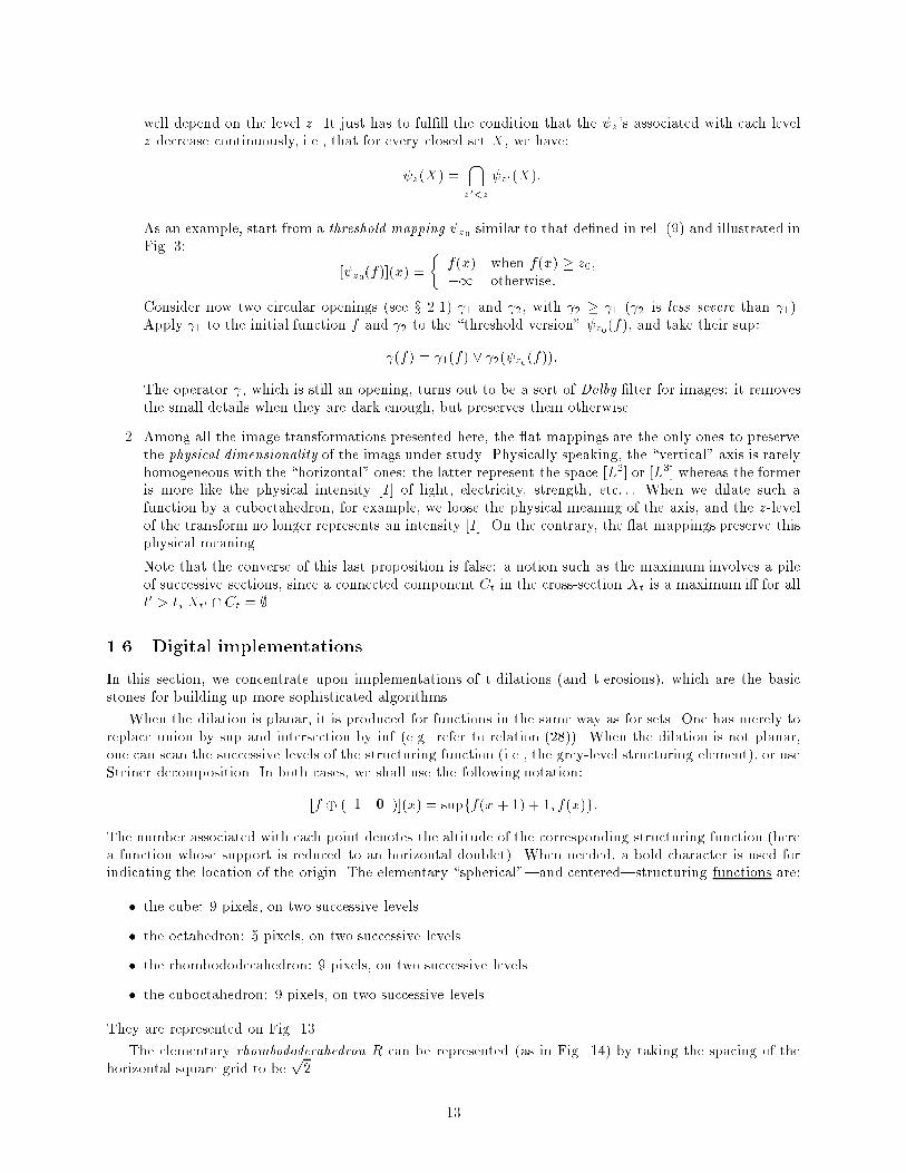
These operations are referred to as planar dilations and erosions, or as dilations and erosions with respectto a planar structuring element B. An example of such transformations is shown in Fig. 12.

f

f

(a) (b)

Figure 12: Dilation (a) and erosion (b) of a function f by a planar structuring element B.

Comments

1. In the example of rel. (28), all the horizontal cross-sections are processed by the same operator, namelythe dilation by B. Such a vertical invariance is not compulsory, and a stack increasing operator may

12

well depend on the level z. It just has to ful�ll the condition that the z's associated with each levelz decrease continuously, i.e., that for every closed set X, we have:

z(X) =\z0<z

z0 (X):

As an example, start from a threshold mapping z0 similar to that de�ned in rel. (9) and illustrated inFig. 3:

[ z0(f)](x) =

�f(x) when f(x) � z0;�1 otherwise:

Consider now two circular openings (see x 2.1) 1 and 2, with 2 � 1 ( 2 is less severe than 1).Apply 1 to the initial function f and 2 to the \threshold version" z0(f), and take their sup:

(f) = 1(f) _ 2( z0(f)):

The operator , which is still an opening, turns out to be a sort of Dolby �lter for images: it removesthe small details when they are dark enough, but preserves them otherwise.

2. Among all the image transformations presented here, the at mappings are the only ones to preservethe physical dimensionality of the imags under study. Physically speaking, the \vertical" axis is rarelyhomogeneous with the \horizontal" ones: the latter represent the space [L2] or [L3] whereas the formeris more like the physical intensity [I] of light, electricity, strength, etc: : : When we dilate such afunction by a cuboctahedron, for example, we loose the physical meaning of the axis, and the z-levelof the transform no longer represents an intensity [I]. On the contrary, the at mappings preserve thisphysical meaning.

Note that the converse of this last proposition is false: a notion such as the maximum involves a pileof successive sections, since a connected component Ct in the cross-section Xt is a maximum i� for allt0 > t, Xt0 \Ct = ;.

1.6 Digital implementations

In this section, we concentrate upon implementations of t-dilations (and t-erosions), which are the basicstones for building up more sophisticated algorithms.

When the dilation is planar, it is produced for functions in the same way as for sets. One has merely toreplace union by sup and intersection by inf (e.g. refer to relation (28)). When the dilation is not planar,one can scan the successive levels of the structuring function (i.e., the grey-level structuring element), or useSteiner decomposition. In both cases, we shall use the following notation:

[f � ( 1 0 )](x) = supff(x + 1) + 1; f(x)g:

The number associated with each point denotes the altitude of the corresponding structuring function (herea function whose support is reduced to an horizontal doublet). When needed, a bold character is used forindicating the location of the origin. The elementary \spherical"|and centered|structuring functions are:

� the cube: 9 pixels, on two successive levels

� the octahedron: 5 pixels, on two successive levels

� the rhombododecahedron: 9 pixels, on two successive levels

� the cuboctahedron: 9 pixels, on two successive levels.

They are represented on Fig. 13.

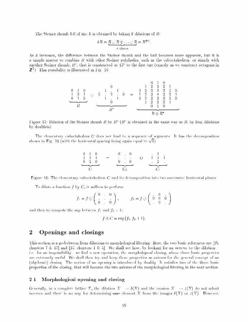
The elementary rhombododecahedron R can be represented (as in Fig. 14) by taking the spacing of thehorizontal square grid to be

p2.

13

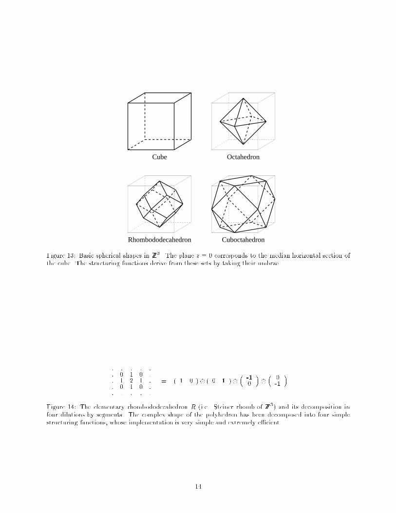
Cube Octahedron

Rhombododecahedron Cuboctahedron

Figure 13: Basic spherical shapes in ZZ3. The plane z = 0 corresponds to the median horizontal section of

the cube. The structuring functions derive from these sets by taking their umbrae.

: : : : :: 0 1 0 :: 1 2 1 :: 0 1 0 :: : : : :

= ( 1 0 ) � ( 0 1 )��-10

���

0-1

�

Figure 14: The elementary rhombododecahedron R (i.e. Steiner rhomb of ZZ3) and its decomposition infour dilations by segments. The complex shape of the polyhedron has been decomposed into four simplestructuring functions, whose implementation is very simple and extremely e�cient.

14

The Steiner rhomb kR of size k is obtained by taking k dilations of R:

kR = R� R� : : :� R| {z }k times

= R�k:

As k increases, the di�erence between the Steiner rhomb and the ball becomes more apparent, but it isa simple matter to combine R with other Steiner polyhedra, such as the cuboctahedron, or simply withanother Steiner rhomb, R�, that is constructed at 45� to the �rst one (exactly as we construct octagons inZZ

2). This possibility is illustrated in Fig. 15.

0 1 01 2 10 1 0| {z }

R

�0

1 : 10 : 2 : 0

1 : 10| {z }R�

=

0 1 01 2 2 2 1

0 2 3 3 3 2 01 2 3 4 3 2 10 2 3 3 3 2 0

1 2 2 2 10 1 0| {z }R� R�

Figure 15: Dilation of the Steiner rhomb R by R� (R� is obtained in the same way as R, by four dilationsby doublets).

The elementary cuboctahedron C does not lead to a sequence of segments. It has the decompositionshown in Fig. 16 (with the horizontal spacing being again equal to

p2).

0 1 01 1 10 1 0| {z }

C

=0 : 0: : :0 : 0| {z }C0

[: 1 :1 1 1: 1 :| {z }C1

Figure 16: The elementary cuboctahedron C and its decomposition into two successive horizontal planes.

To dilate a function f by C, it su�ces to perform

f1 = f �

0 : 0: : :0 : 0

!; f2 = f �

: 0 :0 0 0: 0 :

!

and then to compute the sup between f1 and f2 + 1:

f �C = supff1; f2 + 1g:

2 Openings and closings

This section is a go-between from dilations to morphological �ltering. Here, the two basic references are [25,chapters 7 & 17] and [15, chapters 1 & 5]. We shall see how, by looking for an inverse to the dilation|i.e. for an impossibility|we �nd a new operation, the morphological closing, whose three basic propertiesare extremely useful. We shall then try and keep these properties as axioms for the general concept of an(algebraic) closing. The notion of an opening is introduced by duality. It satis�es two of the three basicproperties of the closing, that will become the two axioms of the morphological �ltering in the next section.

2.1 Morphological opening and closing

Generally, in a complete lattice T , the dilation X �! �(X) and the erosion X �! "(X) do not admitinverses and there is no way for determining one element X from the images �(X) or "(X). However,

15

starting from a dilation and then performing the dual erosion (or the contrary), we always have either anupper, or a lower bound according to the situation at hand.

Indeed, if we take �(X) for the set Y in relation (12), the left inclusion is satis�ed, so X � "�(X), andby duality:

� � "(X) � X � " � �(X);

or in terms of operators:�" � I � "�:

We say that "� is extensive (larger than the identity mapping) and that �" is anti-extensive. Bothoperations are also increasing as the product of increasing mappings. Now, "� � I implies, by growth, that�"�" � �", whereas �" � I implies the inverse inequality. Hence �" = �"�", i.e. is idempotent (as well as"�, by duality). The three properties of "� characterize what is called a closing, in algebra, and those of�" an opening. We shall call these two operators morphological to indicate that they are generated from adilation and its dual erosion, and we denote:

m = �" 'm = "� (30)

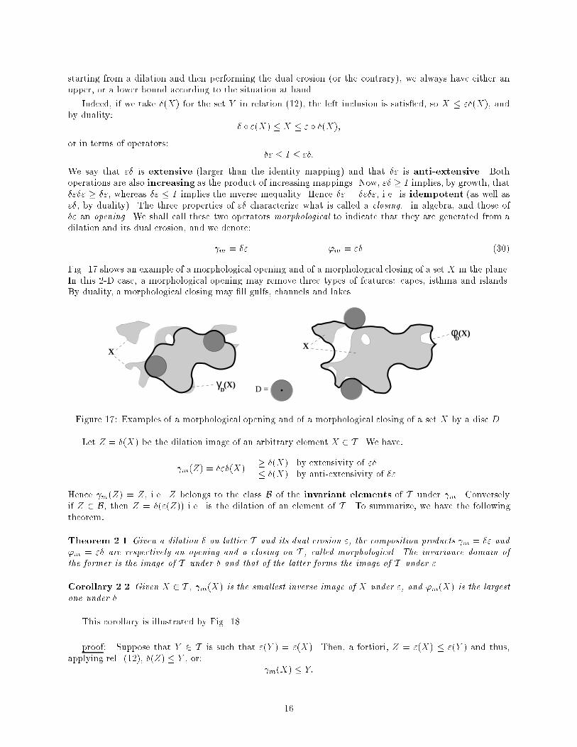
Fig. 17 shows an example of a morphological opening and of a morphological closing of a set X in the plane.In this 2-D case, a morphological opening may remove three types of features: capes, isthma and islands.By duality, a morphological closing may �ll gulfs, channels and lakes.

D =

X

γD

X

(X)

φD(X)

Figure 17: Examples of a morphological opening and of a morphological closing of a set X by a disc D.

Let Z = �(X) be the dilation image of an arbitrary element X 2 T . We have:

m(Z) = �"�(X)� �(X) by extensivity of "�� �(X) by anti-extensivity of �"

Hence m(Z) = Z, i.e. Z belongs to the class B of the invariant elements of T under m. Converselyif Z 2 B, then Z = �("(Z)) i.e. is the dilation of an element of T . To summarize, we have the followingtheorem:

Theorem 2.1 Given a dilation � on lattice T and its dual erosion ", the composition products m = �" and'm = "� are respectively an opening and a closing on T , called morphological. The invariance domain ofthe former is the image of T under � and that of the latter forms the image of T under ".

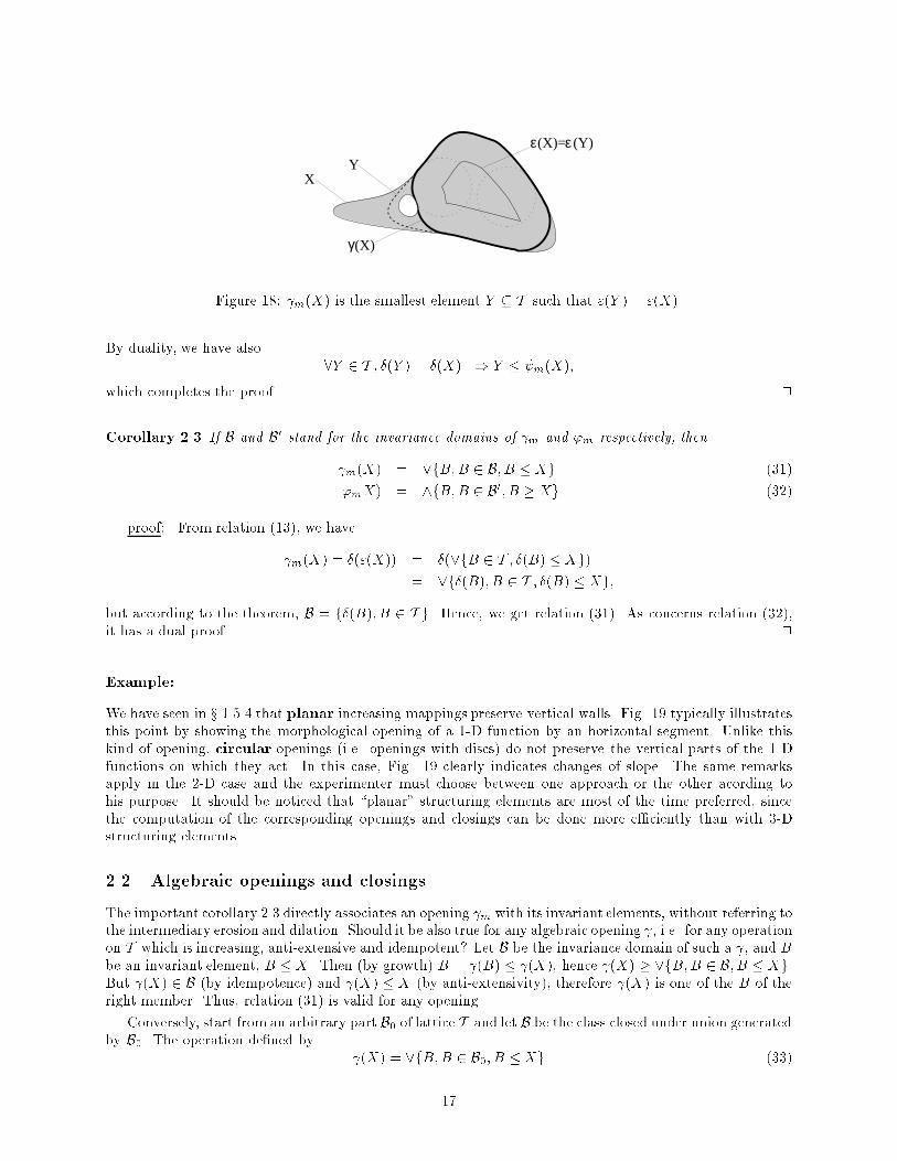
Corollary 2.2 Given X 2 T , m(X) is the smallest inverse image of X under ", and 'm(X) is the largestone under �.

This corollary is illustrated by Fig. 18.

proof: Suppose that Y 2 T is such that "(Y ) = "(X). Then, a fortiori, Z = "(X) � "(Y ) and thus,applying rel. (12), �(Z) � Y , or:

m(X) � Y:

16

ε ε (X)= (Y)

XY

(X)γ

Figure 18: m(X) is the smallest element Y � T such that "(Y ) = "(X).

By duality, we have also8Y 2 T ; �(Y ) = �(X) =) Y � m(X);

which completes the proof. 2

Corollary 2.3 If B and B0 stand for the invariance domains of m and 'm respectively, then

m(X) = _fB;B 2 B; B � Xg (31)

'mX) = ^fB;B 2 B0; B � Xg (32)

proof: From relation (13), we have

m(X) = �("(X)) = �(_fB 2 T ; �(B) � Xg)= _f�(B); B 2 T ; �(B) � Xg;

but according to the theorem, B = f�(B); B 2 T g. Hence, we get relation (31). As concerns relation (32),it has a dual proof. 2

Example:

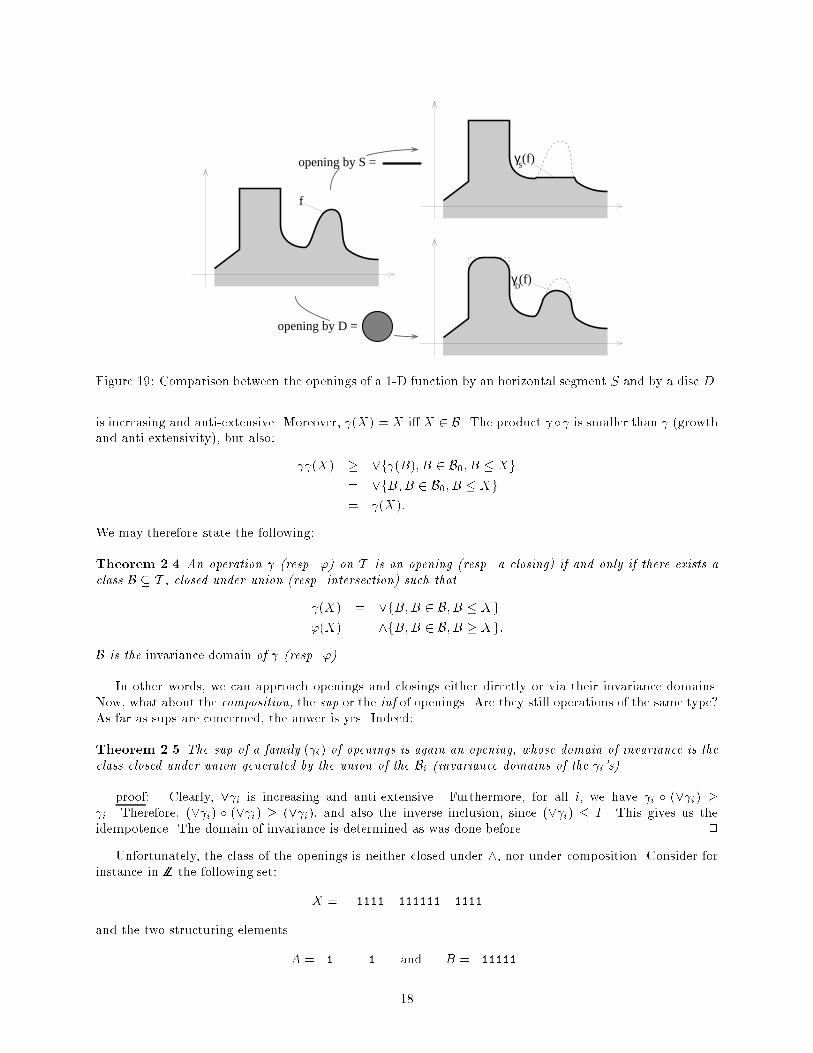
We have seen in x 1.5.4 that planar increasing mappings preserve vertical walls. Fig. 19 typically illustratesthis point by showing the morphological opening of a 1-D function by an horizontal segment. Unlike thiskind of opening, circular openings (i.e. openings with discs) do not preserve the vertical parts of the 1-Dfunctions on which they act. In this case, Fig. 19 clearly indicates changes of slope. The same remarksapply in the 2-D case and the experimenter must choose between one approach or the other acording tohis purpose. It should be noticed that \planar" structuring elements are most of the time preferred, sincethe computation of the corresponding openings and closings can be done more e�ciently than with 3-Dstructuring elements.

2.2 Algebraic openings and closings

The important corollary 2.3 directly associates an opening m with its invariant elements, without referring tothe intermediary erosion and dilation. Should it be also true for any algebraic opening , i.e. for any operationon T which is increasing, anti-extensive and idempotent? Let B be the invariance domain of such a , and Bbe an invariant element, B � X. Then (by growth) B = (B) � (X), hence (X) � _fB;B 2 B; B � Xg.But (X) 2 B (by idempotence) and (X) � X (by anti-extensivity), therefore (X) is one of the B of theright member. Thus, relation (31) is valid for any opening.

Conversely, start from an arbitrary part B0 of lattice T and let B be the class closed under union generatedby B0. The operation de�ned by

(X) = _fB;B 2 B0; B � Xg (33)

17

f

(f)opening by S = γS

(f)γD

opening by D =

Figure 19: Comparison between the openings of a 1-D function by an horizontal segment S and by a disc D.

is increasing and anti-extensive. Moreover, (X) = X i� X 2 B. The product � is smaller than (growthand anti-extensivity), but also:

(X) � _f (B); B 2 B0; B � Xg= _fB;B 2 B0; B � Xg= (X):

We may therefore state the following:

Theorem 2.4 An operation (resp. ') on T is an opening (resp. a closing) if and only if there exists aclass B � T , closed under union (resp. intersection) such that

(X) = _fB;B 2 B; B � Xg'(X) = ^fB;B 2 B; B � Xg:

B is the invariance domain of (resp. ').

In other words, we can approach openings and closings either directly or via their invariance domains.Now, what about the composition, the sup or the inf of openings. Are they still operations of the same type?As far as sups are concerned, the anwer is yes. Indeed:

Theorem 2.5 The sup of a family ( i) of openings is again an opening, whose domain of invariance is theclass closed under union generated by the union of the Bi (invariance domains of the i's).

proof: Clearly, _ i is increasing and anti-extensive. Furthermore, for all i, we have i � (_ i) � i. Therefore, (_ i) � (_ i) � (_ i), and also the inverse inclusion, since (_ i) � I. This gives us theidempotence. The domain of invariance is determined as was done before. 2

Unfortunately, the class of the openings is neither closed under ^, nor under composition. Consider forinstance in ZZ the following set:

X = ..1111..111111..1111...

and the two structuring elements

A = .1.....1. and B = .11111.

18

Denoting Aand

B, the associated morphological openings, we have:

A(X) = X and

B(X) = .111111.

and B�

A(X) =

B(X) 6=

A�

B(X) = ;:

Hence:(

B A)(

B A) 6= (

B A);

and(

B^

A)(

B^

A)(X) = ; 6= (

B^

A)(X) =

B(X):

2

Let us quote a last result which clari�es the links between morphological and algebraic openings:

Theorem 2.6 A mapping : T �! T is an opening if and only if it is the sup of a family ( i) ofmorphological openings. Moreover, if a translation is de�ned over T , is translation invariant if and onlyif the i are translation invariant (dual statement for the closings).

proof: Easy, refer to [15, page 190], [24, page 161], [25, page 22]. 2

2.3 (Non exhaustive) catalog of openings and closings

Although theorem 2.6 is heuristically deep, we may have di�culties in applying it directly, as the number ofterms i necessary for generating a given becomes prohibitive. Actually, there are four starting points forcreating openings, namely:

� the morphological openings,

� the trivial openings,

� the connected openings,

� the envelope openings.

: : :plus any derivation obtained by cross-union of these various types. The �rst mode has already beendeveloped. We will now present the other three.

2.3.1 Trivial openings

A criterion T is said to be increasing when, for all X 2 T :�X satis�es T and Y � X =) Y satis�es T;X does not satisfy T and Y � X =) Y does not satisfy T:

For example, in IRn, for X to hit a given set A0, as well as to have a Lebesgue measure larger than a givenvalue �0 are both increasing criteria.

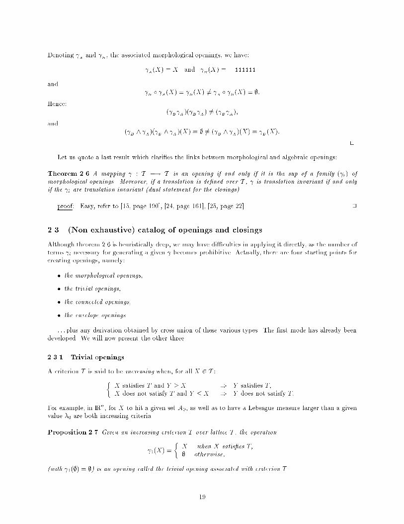
Proposition 2.7 Given an increasing criterion T over lattice T , the operation

1(X) =

�X when X satis�es T;; otherwise:

(with 1(;) = ;) is an opening called the trivial opening associated with criterion T .

19

2.3.2 Connected opening x

We consider a boolean lattice P(E) and an arbitrary point x 2 E. A part C of P(E) is called a connectedclass on P(E) when it satis�es:

(i) ; 2 C and 8x 2 E, fxg 2 C,(ii) For every family (Ci) in C, \Ci 6= ; =) [Ci 2 C.

One proves then [25, page 52] that the datum of a connected class C on P(E) is equivalent to the familyof openings x such that:

(iii) 8x 2 E, x(fxg) = fxg,(iv) 8A � E, x; y 2 E, x(A) and y(A) are equal or disjoint, i.e.

x(A) \ y(A) 6= ; =) x(A) = y(A);

(v) 8A � E; 8x 2 E, x 62 A =) x(A) = ;:

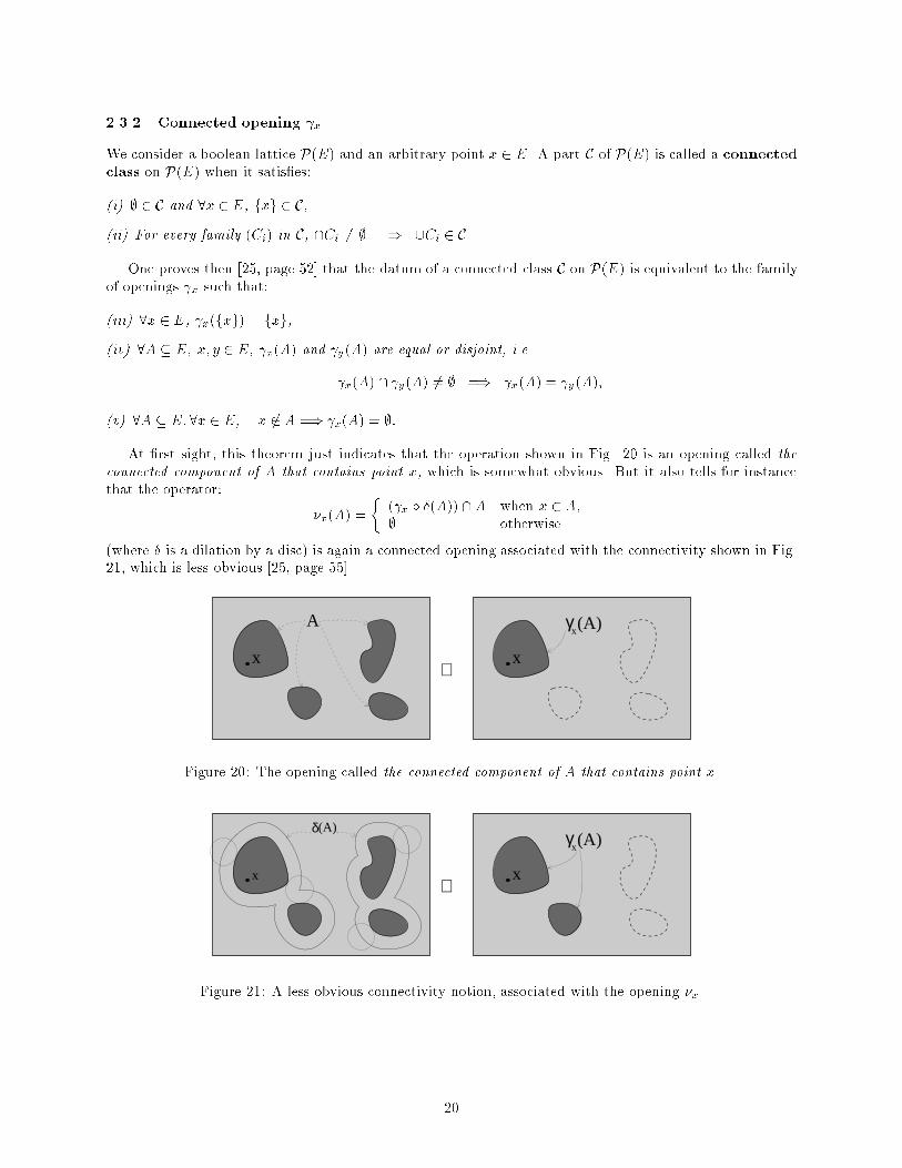
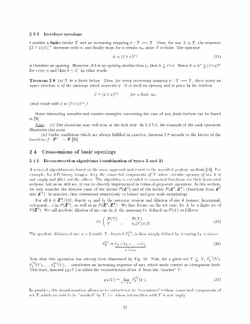
At �rst sight, this theorem just indicates that the operation shown in Fig. 20 is an opening called theconnected component of A that contains point x, which is somewhat obvious. But it also tells for instancethat the operator:

�x(A) =

�( x � �(A)) \A when x 2 A;; otherwise.

(where � is a dilation by a disc) is again a connected opening associated with the connectivity shown in Fig.21, which is less obvious [25, page 55].

A

x x

γ (A)x

⇒

Figure 20: The opening called the connected component of A that contains point x.

γ (A)x

⇒x

(A)

x

δ

Figure 21: A less obvious connectivity notion, associated with the opening �x.

20

2.3.3 Envelope openings

Consider a �nite lattice T and an increasing mapping : T �! T . Then, for any X 2 T , the sequence[X \ (X)]n decreases with n, and �nally stops for a certain n0, since T is �nite. The operator

� = (I ^ )n0 (34)

is therefore an opening. Moreover, if h is an opening smaller than , then h � I^ . Hence h = hn � (I^ )nfor every n and thus h � � . In other words:

Theorem 2.8 Let T be a �nite lattice. Then, for every increasing mapping : T �! T , there exists anupper envelope � of the openings which minorate . It is itself an opening and is given by the relation

� = (I ^ )n0 for a �nite n0:

(dual result with = (I _ )n0 .)

Some interesting remarks and counter-examples concerning the case of non �nite lattices can be foundin [5].

Note: (i) The iterations may well stop at the �rst step. In x 3.5.3, the example of the rank-operatorsillustrates this point.

(ii) Under conditions which are always ful�lled in practice, theorem 2.8 extends to the lattice of thefunctions f : ZZn �! ZZ [26].

2.4 Cross-unions of basic openings

2.4.1 Reconstruction algorithms (combination of types 2 and 3)

A series of algorithms are based on the same approach and resort to the so-called geodesic methods [10]. Forexample, for 2-D binary images: keep the connected components of X whose circular opening of size k isnot empty and �lter out the others. The algorithm is extended to numerical functions via their horizontalsections, but as we will see, it can be directly implemented in terms of grey-scale operators. In this section,we only consider the discrete cases of the lattice P(ZZ2) and of the lattice F(ZZ2;ZZ+) (functions from ZZ

2

into ZZ+). In practice, they correspond respectively to binary and grey-scale morphology.

For all k 2 ZZ+=f0g, denote "k and �k the isotropic erosion and dilation of size k (square, hexagonal,

octogonal: : :) in P(ZZ2), as well as in F(ZZ2;ZZ+). We �rst focuse on the set case: let X be a �nite set ofP(ZZ2). We call geodesic dilation of size one in X the mapping �X de�ned on P(X) as follows:

�X

� P(X) �! P(X)Y 7�! �1(Y ) \X: (35)

The geodesic dilation of size n > 0 inside X, denoted �(n)X , is then simply de�ned by iterating �X n times:

�(n)X = �X � �X � : : : � �X| {z }

n times

: (36)

Note that this operation has already been illustrated by Fig. 10. Now, for a given set Y � X, �(1)X (Y ),

�(2)X (Y ),: : : , �(k)X (Y ): : : constitutes an increasing sequence of sets, which tends toward an idempotent limit.This limit, denoted �X (Y ) is called the reconstruction of set X from the \marker" Y :

�X (Y ) = limk!+1

�(k)X (Y ): (37)

In practice, this transformation allows us to extract|or to \reconstruct"|those connected components ofset X which are said to be \marked" by Y , i.e. whose intersection with Y is not empty.

21

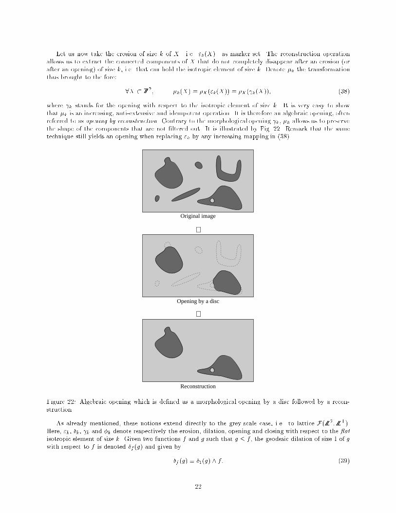
Let us now take the erosion of size k of X|i.e. "k(X)|as marker set. The reconstruction operationallows us to extract the connected components of X that do not completely disappear after an erosion (orafter an opening) of size k, i.e. that can hold the isotropic element of size k. Denote �k the transformationthus brought to the fore:

8X � ZZ2; �k(X) = �X ("k(X)) = �X ( k(X)); (38)

where k stands for the opening with respect to the isotropic element of size k. It is very easy to showthat �k is an increasing, anti-extensive and idempotent operation. It is therefore an algebraic opening, oftenreferred to as opening by reconstruction. Contrary to the morphological opening k, �k allows us to preservethe shape of the components that are not �ltered out. It is illustrated by Fig. 22. Remark that the sametechnique still yields an opening when replacing "k by any increasing mapping in (38).

⇓

⇓

Original image

Opening by a disc

Reconstruction

Figure 22: Algebraic opening which is de�ned as a morphological opening by a disc followed by a recon-struction

As already mentioned, these notions extend directly to the grey-scale case, i.e. to lattice F(ZZ2;ZZ+).Here, "k, �k, k and �k denote respectively the erosion, dilation, opening and closing with respect to the atisotropic element of size k. Given two functions f and g such that g � f , the geodesic dilation of size 1 of gwith respect to f is denoted �f (g) and given by

�f (g) = �1(g) ^ f: (39)

22

Similarly, �(n)f (g) denotes the geodesic dilation of size n of g with respect to f :

�(n)f (g) = (�f � �f � : : : � �f| {z }

n times

)(g) (40)

whereas the reconstruction operation �f is given by the following equation:

�f (g) = limk!+1

�(k)f (g): (41)

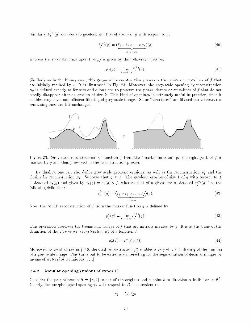
Similarly as in the binary case, this grey-scale reconstruction preserves the peaks or crest-lines of f thatare initially marked by g. It is illustrated in Fig. 23. Moreover, the grey-scale opening by reconstruction�k is de�ned exactly as for sets and allows one to preserve the peaks, domes or crest-lines of f that do nottotally disappear after an erosion of size k. This kind of openings is extremely useful in practice, since itenables very clean and e�cient �ltering of grey-scale images. Some \structures" are �ltered out whereas theremaining ones are left unchanged.

f

g

⇒

Figure 23: Grey-scale reconstruction of function f from the \marker-function" g: the right peak of f ismarked by g and thus preserved in the reconstruction process.

By duality, one can also de�ne grey-scale geodesic erosions, as well as the reconstruction ��f and theclosing by reconstruction ��k. Suppose that g � f . The geodesic erosion of size 1 of g with respect to f

is denoted "f (g) and given by "f (g) = "1(g) _ f , whereas that of a given size n, denoted "(n)f

(g) has thefollowing de�nition:

"(n)f (g) = ("f � "f � : : : � "f| {z }

n times

)(g): (42)

Now, the \dual" reconstruction of f from the marker-function g is de�ned by

��f (g) = limk!+1

"(k)f (g): (43)

This operation preserves the basins and valleys of f that are initially marked by g. It is at the basis of thede�nition of the closing by reconstruction ��k of a function f :

��k(f) = ��f (�k(f)): (44)

Moreover, as we shall see in x 3.6, the dual reconstruction ��f enables a very e�cient �ltering of the minimaof a grey-scale image. This turns out to be extremely interesting for the segmentation of decimal images bymeans of watershed techniques [3, 1].

2.4.2 Annular opening (unions of types 1)

Consider the pair of points B = fo; bg, made of the origin o and a point b in direction � in IR2 or in ZZ2.

Clearly, the morphological opening b with respect to B is equivalent to

b = I ^ �B0

23

where �B0 is the t-dilation by the bi-point B0 = f�b; +bg. Now, make vary b in a certain domain D whichdoes not contain the origin (e.g. three consecutive vertices of an hexagon centered on o, half a circle, : : : )and take the sup :

= _f b; b 2 Dg = I ^ f_�B0 ; b 2 Dgi.e. since the dilation commutes with _:

= I ^ �D[ �D (45)

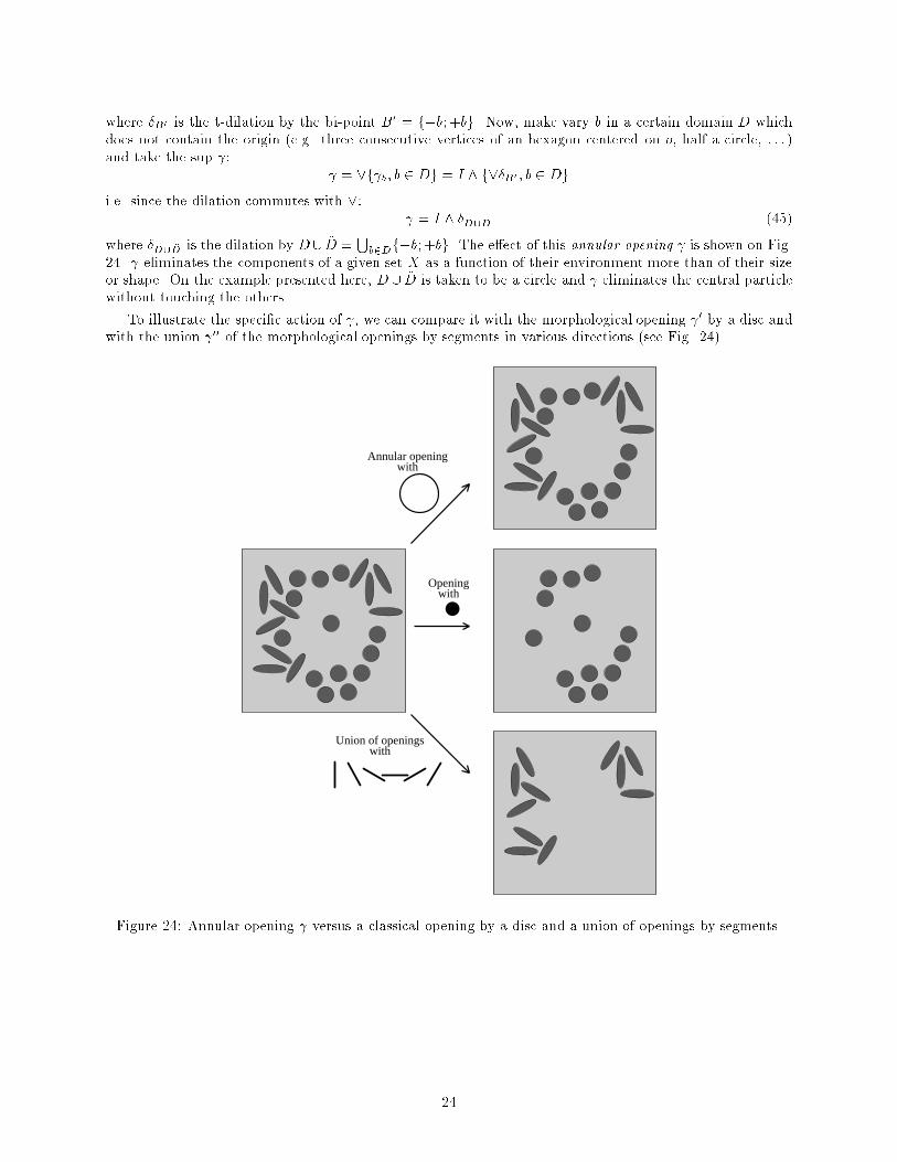
where �D[ �D is the dilation by D[ �D =Sb2Df�b; +bg. The e�ect of this annular opening is shown on Fig.

24. eliminates the components of a given set X as a function of their environment more than of their sizeor shape. On the example presented here, D [ �D is taken to be a circle and eliminates the central particlewithout touching the others.

To illustrate the speci�c action of , we can compare it with the morphological opening 0 by a disc andwith the union 00 of the morphological openings by segments in various directions (see Fig. 24).

Annular openingwith

Openingwith

Union of openingswith

Figure 24: Annular opening versus a classical opening by a disc and a union of openings by segments.

24

3 Morphological �lters

3.1 The lattice of the increasing mappings

This section constitutes an overview of the theory of morphological �ltering, due to G. Matheron [25, chapter6]. The lattice examples introduced in x 1 concerned the scenes under study. We will now consider classes ofoperations working on these objects. Let be such an operator, i.e. be a mapping from a complete latticeT into itself. We assume that is increasing, i.e. that it preserves the ordering relation of T :

8A;A0 2 T ; A � A0 =) (A) � (A0): (46)

The set T 0 of the increasing mappings on the complete lattice T satis�es the following properties:

1. T 0 is a semi-group for the composition product �, with a unit element, namely the identity mapping I(8A 2 T ; I(A) = A).

2. T 0 is a complete lattice for the ordering relation:

f � g () 8A 2 T ; f(A) � g(A);

since the following identities

(_T 0fi)(A) = _T (fi(A)) and (^T 0fi)(A) = ^T (fi(A))generate a supremum and an in�mum in the set T 0.

The two basic structures of the semi-group and of the lattice interact with each other, and we have, forall f , g, h and (fi) in T 0:

(_fi) � g = _(fi � g) ; g � (_fi) � _(g � fi) (47)

(^fi) � g = ^(fi � g) ; g � (^fi) � ^(g � fi) (48)

and

f � g =)�f � h � g � hh � f � h � g

In the following, the two classes of the over�lters (i.e. the mappings f 2 T 0 such that f � f � f) and of theunder�lters play a major role. Indeed:

Theorem 3.1 the class of the under�lters (resp. over�lters) is closed under ^ (resp. _) and under self-composition.

For example, let (fj)j2J be a family of under�lters. From (46) and (48), we get:

(^j2Jfj) � (^j2Jfj) = ^i2J (fi � ^j2Jfj) � ^i2J (fi � fi) � ^i2Jfi;so that ^j2Jfj is an under�lter. Moreover, given an under�lter f , ff � f implies, by growth, that ff �ff �ff , so that the self-composition ff is an under�lter.

3.2 Morphological �lters: de�nition

Following G. Matheron and J. Serra [25, chapters 5{6], we de�ne the notion of a morphological �lter asfollows:

De�nition 3.2 The elements of T 0 which are both under�lters and over�lters are called (morphological)�lters.

25

Note that in literature, the term \�lter" may also be associated with growth only [12, 13], and can evenbe a synonymous with mapping [37]. Here however, the morphological �lters are the transformations actingon the scenes under study (i.e. the lattice T ) which are increasing and idempotent. We shall denote byV the class of the �lters, with V � T 0. Remark that the class V is not closed either under _, or ^, or undercomposition (a counter-example, based on openings, has been brought to the fore in x 2.2).

This apparent drawback suggests us to investigate more accurately the possible connections of class Vwith the composition product and with extrema. Can we �nd, for example, pairs (f; g) of �lters such thatf � g, g � f , f � g � f , etc: : : are surely �lters (composition problem)? Can we keep the usual ordering relationin V and equip V with new sup and inf, such that it turns out to become a complete lattice (extremaproblem)? These two sorts of questions constitute the subject of sections 3.3 and 3.4.

3.3 Composition of morphological �lters

With any increasing mapping : T �! T , associate:

1. the image domain (T ), i.e. the set of the transforms by :

(T ) = f (A); A 2 T g;

2. the invariance domain B , i.e. the class of those B 2 T which are left unchanged under :

B = fB 2 T ; (B) = Bg:

When is a �lter, B is often called the root of in literature.

We always have B � (T ), an inclusion which becomes an equality

B = (T )

if and only if is idempotent. This preliminary remark leads to the following two criteria:

Criterion 3.3 For any mappings f , g from T into itself,

fg = g () g(T ) � Bf :

In particular, when g is idempotent:fg = g () Bg � Bf : (49)

Criterion 3.4 Two mappings f and g from T into itself are idempotent and admit the same invariancedomain Bf = Bg if and only if:

fg = g and gf = f: (50)

Proofs: criterion 3.3 is obvious. Now, if rel. (50) is satis�ed, then ff = f � gf = gf = f , i.e. f , andsimilarly g, are idempotent. Hence, from (49), Bf � Bg and Bg � Bf . Conversely, when f and g, idempotent,have the same invariance domain, rel. (50) is nothing but (3.4). 2

In these two criteria, the ordering � does not intervene. From now on, we shall only consider theincreasing mappings , i.e. the mappings 2 T 0. For any �lter , the class of the �lters 0 that havethe same invariance domain B as is denoted Id( ). The following theorem is the key result concerningthe composition of �lters:

Theorem 3.5 (structural theorem) Let f and g be two �lters on T such that f � g. Then:

(i) f � fgf � gf _ fg � gf ^ fg � gfg � g,

(ii) gf , fg, fgf and gfg are �lters, and fgf 2 Id(fg), gfg 2 Id(gf),

26

(iii) fgf is the smallest �lter greater than gf _ fg and gfg is the greatest �lter smaller than gf ^ fg,(iv) the following equivalences hold:

Bfg = Bgf () Bfg = Bf \ Bg () Bgf = Bf \ Bg() fgf = gf () gfg = fg() gf � fg:

proof: The inequalities (i) are obvious.

From the relationshipsfg = fffg � fgfg � fggg = fg;

we conclude that fg is a �lter. By the dual inequalities, gf is also a �lter. Now, we have

fgf � fg = fg(ff)g = fgfg = fg;

fg � fgf = fgfg � f = (fg � fg)f = fgf;

and thus, fgf 2 Id(fg), by criterion 3.4. In the same way, we �nd that fgf 2 Id(gf), so that (ii) is proved.Now, fgf is a �lter (by (ii)) and fgf � gf _ fg (by (i)). Let be a �lter such that � fg and � gf .

It follows that = � fggf = fgf . Thus, fgf is the smallest �ltering upper bound of fg and gf . Hence(iii) is proved.

By criterion 3.4, we have Bfg = Bgf if and only if

fg � gf = fgf = gf and gf � fg = gfg = fg:

These relations actually imply one another. For instance, fgf = gf implies fgf � g = gfgf , i.e. fg = gfg.By (iii), these relations are equivalent to gf � fg.

The inclusionsBf \Bg � Bfg � Bf

always hold, so that Bfg = Bf \ Bg if and only if Bfg � Bg , i.e, by criterion 3.3, if and only if gfg = fg.This completes the proof. 2

Examples:

1. Start from an arbitrary opening and an arbitrary closing �. Since

� I � �;

by theorem 3.5, �, � , � and � � are �lters. The composition products of � by , then by �,etc: : : generates the oscillating sequence

� �! � �! � � �! � �! : : :

Remark that when � � � (which is generally not the case), we have � = � � and the oscillationsare stopped after the �rst step.

2. There is a more particular example, which illustrates point (iv) of the theorem. In P(IRn) (or P(ZZn),or F(IRn; IR), or F(ZZn;ZZ)), consider the morphological opening l by a segment of length l in thehorizontal direction. For a given X, l(X) is made of horizontal segments of length � l. Moreover,closing this set by the dual closing �l, i.e. determining �l l(X) may only suppress intervals between twosuch segments, hence increase the length of the horizontal intercepts; Therefore, l�l l(X) = �l l(X),and by the theorem, �l l � l�l.

27

3.4 The lattice of the �lters

We now go back to the structure of the set V of the �lters acting on lattice T . Clearly, if ( i) is a family ofelements of V, then _ i is an over�lter,

(_i i)(_i i) = _i( i(_j j)) � _i( i � i) = _i i;

and similarly,^ i is an under�lter. Since _ i is an over�lter, the class C closed under _ and self-compositiongenerated by _ i only comprises over�lters (theorem 3.1). It admits a largest element f , for T 0 is a completelattice. But f � f also belongs to C (closure under self-composition), hence f � f � f , i.e. f is a �lter.

Consider now a �lter 0 larger than _ i. The class C0 of the over�lters smaller than 0 is, in turn, closedunder _ and self-composition, and contains the previous class C. Hence, f � 0, i.e. f turns out to be thesmallest �lter which majorates the i's. By duality, we have a similar result for the inf, and we may state:

Theorem 3.6 The set V of the �lters on T is a complete lattice. For any family ( i) of �lters on T , thesmallest �lter greater than _ i is the largest element f of the class closed under _ and self-compositiongenerated by ( i). Dual result for the largest �lter smaller than ^ i.

In particular, when T is �nite, we always have, for a large enough n:

f = (_ i)n; (51)

a result which provides the algorithm for computing f in practice. Refer to [5] for some counter-examplesin the case where T is not a �nite lattice.

Examples:

1. Lattice of the openings: take the class V0 � V of the openings on T . We have seen that for every family( i) in V0, _ i is still an opening (theorem 2.5). Moreover, from theorem 3.6, there exists a largest�lter g which is smaller than all the i's. g being obviously anti-extensive, V0 is a complete lattice.

2. Start from an arbitrary increasing mapping . Then, the extensive mapping I _ is an over�lter andthe proof of the theorem shows that there exists a smaller �lter |hence a smaller closing|thatmajorates . In the �nite case, we �nd again theorem 2.8.

3.5 _- and ^-�lters, � and � , strong �lters

3.5.1 Introduction

We say that a mapping f : T �! T is a _-mapping when

f = f � (I _ f) (52)

and a ^-mapping whenf = f � (I ^ f): (53)

Basically, this property is something new and independent from the two axioms which build the de�nitionof the morphological �lters. If now f is increasing and satis�es rel. (52), we shall call it a _-under�lter.Indeed, any _-under�lter is an under�lter and similarly, any ^-over�lter is an over�lter. If f is, for instance,a _-under�lter, then we have:

f = f � (I _ f) � f _ ff � f:

Thus, f = f _ ff is an under�lter.

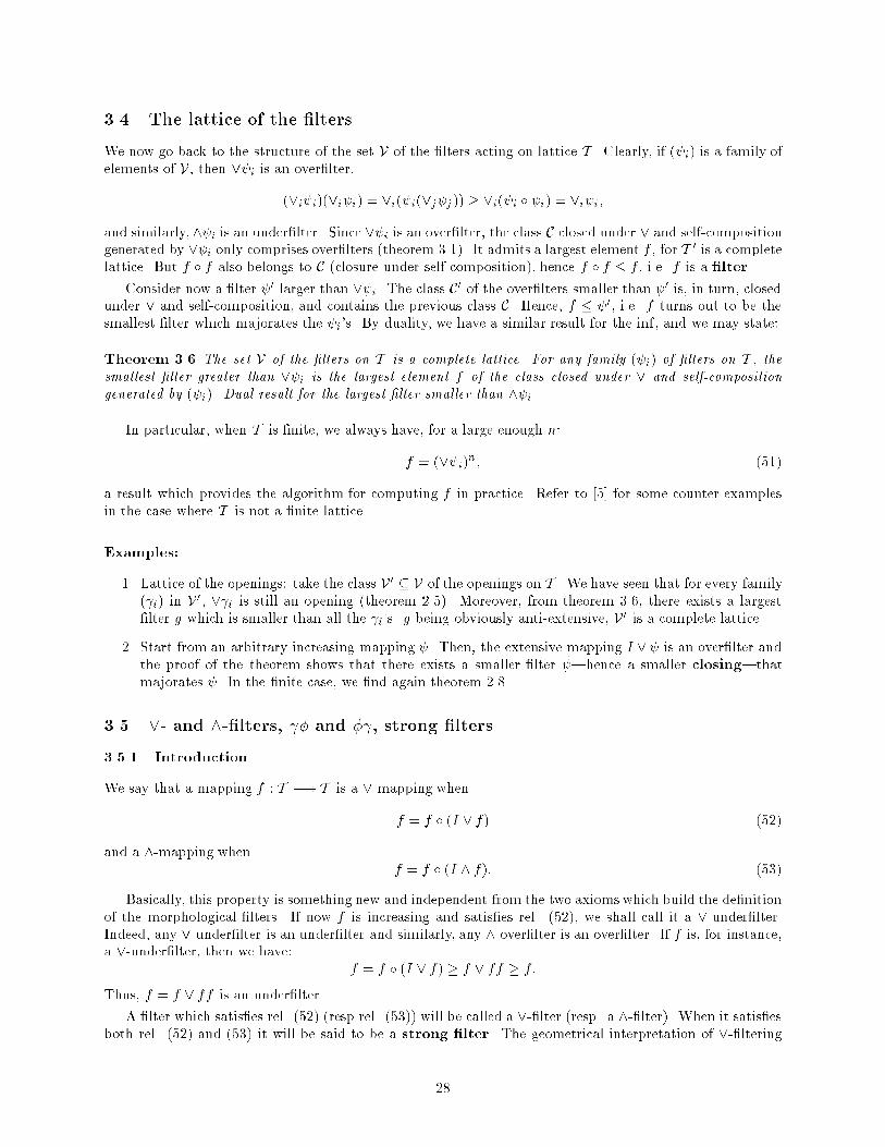
A �lter which satis�es rel. (52) (resp rel. (53)) will be called a _-�lter (resp. a ^-�lter). When it satis�esboth rel. (52) and (53) it will be said to be a strong �lter. The geometrical interpretation of _-�ltering

28

and of ^-�ltering are very easy. Indeed, is a _-�lter if and only if, for any A 2 T , every B between A andA _ (A) has the same transform as A itself (see Fig. 25), i.e.

_��lter: 8A 2 T ; (A � B � A _ (A) =) (B) = (A)):

Similarly, we have

^��lter: 8A 2 T ; (A ^ (A) � B � A =) (B) = (A)):

A

Ψ( )=Ψ( )A B

B

A

Ψ( )=Ψ( )A B

B

(a) (b)

Figure 25: An example of a _-�lter (a) and of a strong �lter (b).

The following result corresponds to the theorem 3.1 of the general case|and is proved in the same way:

Theorem 3.7 the class of the _-under�lters (resp. ^-over�lters) is closed under ^ (resp. under _) andself-composition.

(Note the chiasma; it is the sup and not the inf of ^-over�lters which is still an ^-over�lter.) Thistheorem suggests us to approach �rst the properties of self-composition, and then that of sup and inf, justas we did in the general case.

3.5.2 Composition of _- and ^-�ltersTheorem 3.8 Let f and g be two �lters on T and f � g. Then

(i) if f is a _-�lter, gf and fgf are _-�lters,(ii) if f is a ^-�lter, fg and gfg are ^-�lters,(iii) if gf is a ^-�lter, fgf is a ^-�lter,(iv) if fg is a _-�lter, gfg is a _-�lter.

proof: Easy [25, page 119]. 2

Example: If is an opening and � a closing, we have � I � �, and then

� and � are strong �lters,

� � and � � are _-�lters,� � and � are ^-�lters.

Moreover, if � is a ^-�lter, and thus a strong �lter, � � is a strong �lter. In the same way, if � is a strong�lter, then � is a strong �lter.

29

3.5.3 The two envelopes and �

In x 3.4, we have associated with each 2 T 0 the largest opening � that minorates and the smallestclosing which majorates . These two primitives play a central role in the _- and ^-characterizations, asis shown by the following theorem:

Theorem 3.9 An increasing mapping : T �! T is a _-under�lter (resp. a ^-over�lter) if and only if

= (resp. = � ).

proof: If = (I _ ), then(I _ )(I _ ) = I _ _ (I _ ) = I _ _ = I _ :

The mapping I _ , which is idempotent and which majorates I, is nothing but , and (I _ ) = .

Conversely, start from � (I _ ) � (I _ ) = ;

which implies = (I _ ). Now, if = , then

= = (I _ ) = (I _ ). 2

Corollary 3.10 If 2 T 0 is an over�lter (resp. an under�lter), then is the smallest _-�lter whichmajorates (resp. the largest ^-�lter which minorates ).

proof: If is an over�lter, then

� � � =

and is a �lter. It is also a _-�lter, since � (I _ ) � (I _ ) = ;

which implies (I _ ) = . Finally, if 0 is a _-�lter, with 0 � , then 0 = 0 0 � implies 0 � ,

hence 0 = 0 0 � . 2

Corollary 3.11 When T is a �nite lattice, then

for n large enough, = (I _ )n: (54)

Indeed, corollary 3.10 associates two envelopes with each �lter , so that is �nally surrounded by fourextremum �lters as follows:

� � � � � � : (55)

We have seen that the product � of any closing followed by any opening was a _-�lter. We will provenow that the converse is true, so that the _-property characterizes the class of the �lters of the type �.Theorem 3.12 A mapping 2 T 0 is a _-�lter (resp. a ^-�lter) if and only if there exist an opening anda closing � such that = � (resp. = � ).

proof: Assume that is a _-�lter and consider its invariance domain B. Denote by B~the class closed

for the sup which is generated by B, and by I~the associated opening. Clearly, we have �I

~. Moreover,

according to criterion 3.4, B �B~implies =I

~ and (theorem 3.9) =I

~ . Thus, we may write:

=I~ =I

~

8<:

�I~ for �I

~;

�I~ for � :

Hence, =I~ , i.e. the composition product of a closing by an opening. 2

Remark: the above decomposition is not unique. We also have, for a _-�lter , = � .

30

Example: the rank operators We will illustrate the important theorem 3.9 by considering some prop-erties of the rank operators [19, 8, 20]. Let f be a function from ZZ

n into ZZ and let B � ZZn be a �nite

and symmetrical set of p points implanted at the origin. B is the (moving) window in which the rankingoperation will be implemented. The transform Rk of rank k of f at point x 2 ZZ

n is obtained by orderingthe family (f(y))y2Bx with decreasing values (for example), and by replacing f(x) by the k-th value of thesequence that is thus constructed (1 � k � p). For k = p and k = 1, this leads to Minkowski addition andsubtraction. When k = 1

2(p+1) and p is an odd number, the resulting operation is sometimes called median�ltering, [37] in literature.

The rank operator Rk of rank k is increasing, since it can be decomposed into the sup of the t-erosions"i by all the Bi � B which possess k points:

Rk(f) = _f"i(f); Bi � B;Card(Bi) = kg: (56)

Now, i = �B"i is a ^-over�lter. Indeed:

i i = �B"i�i"i

� � �B"i = i for "i�i � I;

� �B"i = i for �i"i � I;

and i i = i. On the other hand, i � i implies i � I ^ i � I, hence i = i(I ^ i) and �nally, i = i(I ^ i). Rel. (56) shows that �BRk = _ i is still a ^-over�lter (theorem 3.7), and by applicationof theorem 3.9, I ^ �

BRk is an opening (called Ronse opening). In particular, for k = 1, one �nds the

morphological opening by B, and for k = p, the identity I. The other openings increase with k.

As another application of the results presented in this section, one can refer to an interesting study ofF. Meyer [18], where the author directly transcribes into practice and into algorithms the above theorems.Some of the �lters which are thus brought to the fore stem directly from classical median �lters [37]. Besides,in two papers by P. Maragos [12, 13] which are among the most interesting ones in the recent literature onmorphological �lters, one can �nd a thorough study on the relations between morphological �lters andnon-morphological ones, namely median �lters, rank �lters and stack �lters: : :

3.5.4 The lattice of the strong �lters

Starting from an ^-over�lter f 0, the �rst corollary of theorem 3.9 ensures that f = f 0f 0 is an _-�lter. Itwould be excellent if it could also keep the ^-over�ltering property of its primitive f 0. In this case, we wouldhave found the key for producing strong �lters. The answer will actually be positive in the case of modularlattices T , i.e. such that

8A;B;C 2 T ; B � A =) (A _C) ^B = A _ (B ^C)(Except the partition lattice, all the lattices used as models in morphology are modular.). Then, we havethe following lemma:

Lemma 3.13 When T is modular, then

1. f � (I ^ f) is a _-�lter for any _-�lter f ,2. g � (I _ g) is a ^-�lter for any ^-�lter g.

proof: easy. Refer to [25, page 124]. 2

Theorem 3.14 When the lattice T is modular, if f 0 is a ^-over�lter (resp. an ^-under�lter), then f = f 0f 0

(resp. g = g0�g0) is a strong �lter.

proof: Let f 0 be a ^-over�lter and f = f 0f 0. We have

f 0 = f 0(I ^ f 0) � f(I ^ f) � f:

Now, from the lemma, f(I ^ f) is a _-�lter. Since it also majorates f 0, it is larger than the smallest _-�lterwhich majorates f 0, namely f . Hence, f = f(I ^ f) is strong. 2

31

Corollary 3.15 When T is modular, the class of the strong �lters on T is a complete lattice based on theusual ordering. The supremum of a family ( i) of strong �lters is f 0f 0, with f 0 = _ i, and the in�mum isgiven by g0�g0, with g0 = ^ i.

Examples:

1. Theorem 3.14 opens the way for the construction of as many strong �lters as we wish, by iterations. Itsu�ces to start from an arbitrary opening and an arbitrary closing �: when lattice T is �nite, thereexist two integers n and p such that both mappings

= � (I _ � )n and 0 = �(I ^ �)n

are strong �lters.

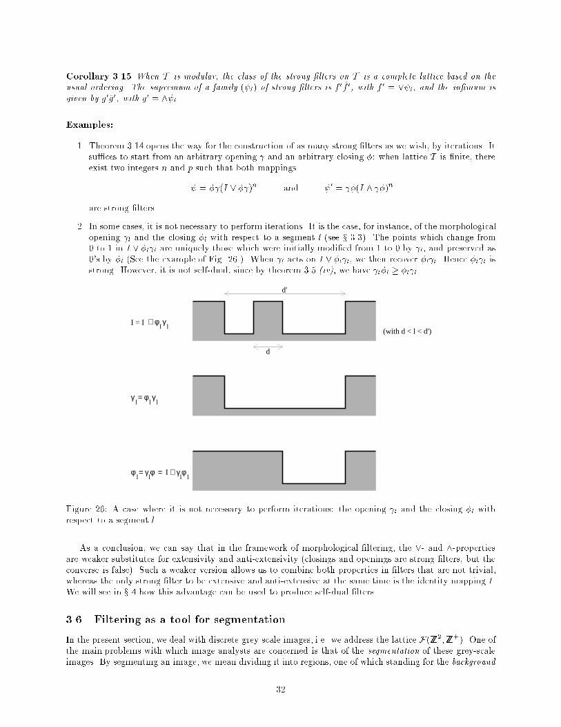
2. In some cases, it is not necessary to perform iterations. It is the case, for instance, of the morphologicalopening l and the closing �l with respect to a segment l (see x 3.3). The points which change from0 to 1 in I _ �l l are uniquely those which were initially modi�ed from 1 to 0 by l, and preserved as0's by �l (See the example of Fig. 26.). When l acts on I _ �l l, we then recover �l l. Hence �l l isstrong. However, it is not self-dual, since by theorem 3.5 (iv), we have l�l � �l l.

d'

d

(with d < l < d')I = I ∨ φ γ

l l

γ = φ γl ll

φ = γ φ = ∨ γ φll l l

I

Figure 26: A case where it is not necessary to perform iterations: the opening l and the closing �l withrespect to a segment l.

As a conclusion, we can say that in the framework of morphological �ltering, the _- and ^-propertiesare weaker substitutes for extensivity and anti-extensivity (closings and openings are strong �lters, but theconverse is false). Such a weaker version allows us to combine both properties in �lters that are not trivial,whereas the only strong �lter to be extensive and anti-extensive at the same time is the identity mapping I.We will see in x 4 how this advantage can be used to produce self-dual �lters.

3.6 Filtering as a tool for segmentation

In the present section, we deal with discrete grey-scale images, i.e. we address the lattice F(ZZ2;ZZ+). One ofthe main problems with which image analysts are concerned is that of the segmentation of these grey-scaleimages. By segmenting an image, we mean dividing it into regions, one of which standing for the background

32

whereas each of the remaining ones represents one of the objects to be extracted. The boundaries of theseregions must be as close as possible to the \true" contours of these objects. Therefore, the segmentationtask we deal with is nothing but a contour detection problem.

The major di�culty is to de�ne the contours of the image I under study at best. The objects to extractare generally light on a dark background, or are dark on a light background. Therefore, one can imaginede�ning their contours as the regions of I where the grey values are varying very fast, i.e. as crest-lines ofthe gradient of this image. Depending on the problem, i.e. on the contours that have to be detected, manydi�erent gradients may be used. In the �eld of mathematical morphology, the most commonly used one isoften referred to as Beucher's gradient [24]: denote � and " respectively the dilation and the erosion withrespect to the at elementary isotropic element (square, hexagon,: : :). The gradient of I is given by

grad(I) = �(I) � "(I); (57)

where � refers to the algebraic di�erence of two functions. In some particular cases, one can also usedirectional gradients, disymmetryc ones like �(I) � I or I � "(I), etc: : : and various combinations of thesedi�erent gradients.

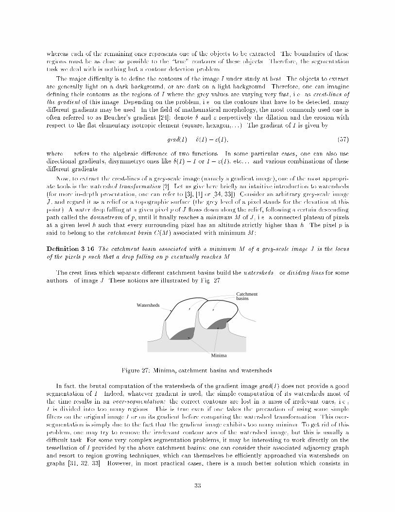
Now, to extract the crest-lines of a grey-scale image (namely a gradient image), one of the most appropri-ate tools is the watershed transformation [2]. Let us give here brie y an intuitive introduction to watersheds(for more in-depth presentation, one can refer to [3], [1] or [34, 33]). Consider an arbitrary grey-scale imageJ , and regard it as a relief or a topographic surface (the grey level of a pixel stands for the elevation at thispoint). A water drop falling at a given pixel p of J ows down along the relief, following a certain descendingpath called the downstream of p, until it �nally reaches a minimumM of J , i.e. a connected plateau of pixelsat a given level h such that every surrounding pixel has an altitude strictly higher than h. The pixel p issaid to belong to the catchment basin C(M ) associated with minimumM :

De�nition 3.16 The catchment basin associated with a minimum M of a grey-scale image J is the locusof the pixels p such that a drop falling on p eventually reaches M .

The crest-lines which separate di�erent catchment basins build the watersheds|or dividing lines for someauthors|of image J . These notions are illustrated by Fig. 27.

Minima

Watersheds

Catchmentbasins

Figure 27: Minima, catchment basins and watersheds.

In fact, the brutal computation of the watersheds of the gradient image grad(I) does not provide a goodsegmentation of I. Indeed, whatever gradient is used, the simple computation of its watersheds most ofthe time results in an over-segmentation: the correct contours are lost in a mass of irrelevant ones, i.e.,I is divided into too many regions. This is true even if one takes the precaution of using some simple�lters on the original image I or on its gradient before computing the watershed transformation. This over-segmentation is simply due to the fact that the gradient image exhibits too many minima. To get rid of thisproblem, one may try to remove the irrelevant contour arcs of the watershed image, but this is usually adi�cult task. For some very complex segmentation problems, it may be interesting to work directly on thetessellation of I provided by the above catchment basins: one can consider their associated adjacency graphand resort to region-growing techniques, which can themselves be e�ciently approached via watersheds ongraphs [31, 32, 33]. However, in most practical cases, there is a much better solution which consists in

33

modifying the gradient function before computing its watersheds. The idea is to make use of grad(I) for theconstruction of a function �(I) whose watersheds provide the desired segmentation.

To achieve this goal, a very powerful method was introduced by F. Meyer, which is detailed in [3]. Ratherthan �ltering out the irrelevant minima of the gradient blindly, this technique assumes that markers of theobjects of I are available. By marker, we mean a connected component of pixels which is included in theobject which is marked. The development of a robust automatic marking procedure may well be an extremelycomplex task, and has to be adapted to each case. Usually, some external knowledge on the collection ofimages under study has to be used. From now on, we assume that a set of markers is available. We alsosuppose that a marker of the background has been brought to the fore.

Let S be the set of pixels of I belonging to one of the above markers. Starting from grad(I), theconstruction of �(I) is done in two steps:

1. Impose as minima the previously extracted markers.

2. Suppress the unwanted minima.

In step 1, we simply construct the function f de�ned by:

8p; f(p) =

�c when p 2 S,grad(I)(p) otherwise,

with c being an arbitrary constant, strictly minorating grad(I).

In the step 2, we have to �lter out the unwanted minima of f , without forgetting to �ll up their associatedwatersheds! To do so, we �rst construct a function, say g, as follows:

8p; g(p) =

�c when p 2 S,A otherwise,

with A being an arbitrary constant majorating grad(I). Then, using the dual grey-scale reconstructionoperation ��f presented in x 2.4.1, we build �(I) as follows:

�(I) = ��f (g):

These two operations are illustrated in Fig. 28.

One can see that the resulting function �(I) is such that its dividing lines correspond exactly to thedesired contours. Indeed, the highest crest-lines of the gradient separating the markers have been preserved.According to the set of markers available and to the gradient which is being used, we therefore have extractedthe best possible contours! Note that, given a set of markers, the transformation (grad(I) 7�! �(I)) is nothingbut a strong �lter: it is indeed the composition product of a closing by an opening, and can as well be de�nedas the composition of an opening by a closing: : : We have thus illustrated how one can develop customized�lters adapted to a speci�c problem|namely the �ltering of unwanted minima. The present method turnsout to be extremely powerful in a number of complex segmentation cases, since the only problem (which canbe itself very complicated!) comes down to detecting the markers of the objects to extract.

4 Granulometries, Alternating Sequential Filters

4.1 Size distributions

Size distributions (also called granulometries) deal with families of openings or closings that are parametrizedby a positive number (the size) [14]. More precisely, we have the following:

De�nition 4.1 A family ( �) of mappings from T into T , depending on a positive parameter � is a size

distribution when

(i) 8� > 0; �is an opening,

34

c

A

Desired minima

Resultingfunction

g

Initialgradient

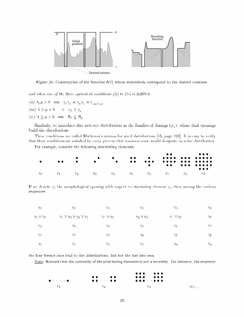
Figure 28: Construction of the function �(I) whose watersheds correspond to the desired contours.

and when one of the three equivalent conditions (ii) to (iv) is ful�lled:

(ii) �; � > 0 =) � �=

� �=

sup(�;�)

(iii) � � � > 0 =) � � �

(iv) � � � > 0 =) B� � B�.

Similarly, we introduce also anti-size distributions as the families of closings ('�), whose dual openings

build size distributions.

These conditions are called Matheron's axioms for sized distributions [15, page 192]. It is easy to verifythat these conditions are satis�ed by every process that common sense would designate as a size distribution.

For example, consider the following structuring elements:

e0 e1 e2 e3 e4 e5 e6 e7 e8 e9

� � � ��

�� �

� � �� � �

� � ��

� �� � � �� � � �� �

� � �� � �� � �

� � �� � � � �� � � � �� � � � �� � �

If we denote i the morphological opening with respect to stucturing element ei, then among the varioussequences

0 0 0 0 0 0

1 _ 2 1 _ 2 _ 3 _ 4 1 _ 2 3 _ 4 1 _ 2 5

5 6 5 5 5 7

7 7 7 8 8 6

9 9 9 9 8 9

the four former ones lead to size distributions, but not the last two ones.

Note: Remark that the convexity of the structuring elements is not a necessity. For instance, the sequence

e1 e2 e3 etc: : :

� �� � � � � �� �

� � � � �� �

� � �� � �� � �

� � � � �� � �� � �

35

induces a size distribution. However, in the Euclidean space IRn, a family (B�)��0 of structuring elementsgenerates a size distribution ( �)��0 which is compatible with the magni�cation, i.e.

8� � 0; 8X � IRn; �(X) = � 1(X=�); (58)

if and only of the B�'s are the homotethics of a compact convex set B. The signi�cation of rel. (58) isclear: it just means that � acts on �X just as 1 does on X. Such a property, which is always satis�ed forconvolution products, may not exist for morphological �lters. However, in the two important cases of thesize distributions and of the alternating sequential �lters (See x 4.2), we easily obtain it.

4.2 Alternating Sequential Filters

This section is devoted to the presentation of a particular class of �lters, namely the alternating sequential�lters (ASF). It provides a simpli�ed version of the results proved in [25, chapter 10]. The theory developedin [25] requires monotonous sequential continuity for covering both continuous and discrete cases. For thesake of simplicity, we restrict ourselves here to the latter case (i.e. P(ZZn), F(ZZn;ZZ) or planar graphs),which allows us to avoid monotonous topology. Furthermore, so as not to bore the reader, most of the proofswill be omitted. They are indeed all very similar to one another and the missing ones can be found in [28,chapter 5].

4.2.1 Introduction

The appearance of some alternating sequential �lters (of Ni type, see below) in the world of mathematicalmorphology is due to an experimental work of Sternberg [30] (the corresponding theoretical developmentsare due to Serra [25, chapter 10]). His study consisted in taking a polyhedric form (namely a cuboctahedron,see x 1.6), altering it by the addition of a largely varying white noise, and then trying to clean the resultingimage X (see [25, page 204]). To attain this goal, X was �rst �ltered by a small closing �1, followed by asmall opening 1, then by a slightly larger closing �2 followed by a slightly larger opening 2, etc: : : The�nal operator produced by this succession of openings and closings was

M = ( i�i) � : : : � ( 2�2) � ( 1�1):The family (�i) that was used in this example consisted in morphological closings by homothetic structuringelements, whereas ( i) was the dual family of openings. After this experiment, a certain number of questionsarose: is the operatorM a �lter? To what extend does it depend on the totality of the sequence of parameters1, 2,: : : , i? Is it essential to use a size distribution ( i) and its dual (�i)? Is the product of these operatorsan operator of the same type?: : :

In this section, a more formal approach of the above operators is proposed. The ASF's of type M arede�ned, as well as other classes of ASF's, namely that of type N , R and S. A number of properties of theseoperators, dealing with composition and order relation, are then given, and the symmetrical sequential �ltersare also presented. The end of the section is concerned with more concrete problems, such as computationtime and practical use of these �lters.

4.2.2 De�nitions

In the following, T denotes a discrete lattice such as P(ZZn) or F(ZZn;ZZ). We also consider two families( i)i�1 and (�i)i�1|indexed on ZZ+=f0g|of operators on T , which are a size distribution and an anti-sizedistribution respectively, i.e:

8i 2 ZZ; i � 1; i is an opening and �i is a closing. (59)

8i; j 2 ZZ; 1 � i � j; j � i � I � �i � �j: (60)

Moreover, we have seen in de�nition 4.1 that the inequalities (60) are equivalent to the following property:

8i; j 2 ZZ; i j = j i = max(i;j) and �i�j = �j�i = �max(i;j) (61)

36

Remark that these two families are chosen independently from one another (although they are often takenas dual of each other in practice).

Now, we know (refer to the structural theorem 3.5) that there are four di�erent ways for composing two�lters f and g such that f � g in order to get new �lters. Therefore, we de�ne for all i 2 ZZ; i � 1, thefollowing operators

mi = i�i ri = �i i�ini = �i i si = i�i i:

(62)

which are �lters (see theorem 3.5). From now on, we give the proofs only for the case of the mi, the othercases being left to the reader.

Proposition 4.2 For i; j 2 ZZ such that 1 � i � j, we have:

mjmi � mj � mimj

�rjririrj

�� rj (63)

ninj � nj � njni

�sjsisisj

�� sj: (64)

proof: from i � I, we obtain i�i � �i � �j. Hence, �j i�i � �j and �nally, mjmi = j�j i�i � j�j = mj , which is the �rst inequality. Similarly, I � �i implies i � i�i. Thus j = i j � i�i j , andmj = j�j � i�i j�j = mimj. This completes the proof. 2

Proposition 4.3 Let (ik)1�k�p be p numbers such that

8k; ik 2 ZZ; 1 � ik � i1 = ip:

then: �mipmip�1 : : :mi2mi1 = mip = mi1

nipnip�1 : : :ni2ni1 = nip = ni1

proof: Easy by using rel. (63). Refer to [28, page 47]. 2

We can now give the de�nition of the alternating sequential �lters and prove that they are e�ectively�lters:

De�nition 4.4 For all i 2 ZZ; i � 1, the following operators:

Mi = mimi�1 : : :m2m1 Ri = riri�1 : : : r2r1Ni = nini�1 : : : n2n1 Si = sisi�1 : : : s2s1

are called alternating sequential �lters of order i.

Proposition 4.5 8i 2 ZZ; i � 1, the operators Mi, Ni, Ri and Si are �lters.

proof: These operators are increasing as compositions of increasing mappings. Moreover, we have:

MiMi = (mimi�1 : : :m2m1mi)(mi�1 : : :m2m1)

= mi(mi�1 : : :m2m1) (by prop. 4.3)

= Mi:

The idempotence of Mi is thus proved. One can also easily show that Ni, Ri and Si are �lters. 2

37

4.2.3 Properties

We have already said that there is no need for duality between the i's and the i's. Anyway, an ASF cannotbe self dual, since Ni 6=Mi. We present below some properties of the ASF's with respect to the compositionproduct and the order relationship between operators : the \absorption laws". We then deal with new �ltersderived from the previous ones and called symmetrical alternating �lters.

Proposition 4.6 (Absorption laws) For i; j 2 ZZ such that 1 � i � j, we have the following relations:

MjMi =Mj � MiMj RiRj � Rj = RjRi; (65)

NiNj � Nj = NjNi SjSi = Sj � SiSj : (66)

proof: similar to that of proposition 4.5. 2

De�nition 4.7 With for all i 2 ZZ; i � 1:

M ti = m1m2 : : :mi�1mi Rti = r1r2 : : : ri�1ri

N ti = n1n2 : : : ni�1ni Sti = s1s2 : : : si�1si

(67)

the following operators:~Mi = M t

iMi~Ri = RtiRi

~Ni = N tiNi

~Si = StiSi(68)

are called alternating symmetrical �lters of order i.

One can easily prove that these operators are indeed �lters. They also satisfy absorption laws and otherproperties, which are listed and proved in [28]. In addition, we have the following theorem :

Theorem 4.8 The set f ~Mi; i 2 ZZ; i � 1g (resp. f ~Ni; i 2 ZZ; i � 1g, f ~Ri; i 2 ZZ; i � 1g, f ~Si; i 2 ZZ; i � 1g)constitutes a commutative semi-group of �lters satisfying the following internal law of composition:

8i � 1; j � 1; ~Mi~Mj = ~Msup(i;j):

Note that, apart from the above ones, the only known semi-groups of this type are the granulometries.

Within each of the four types of operations that we have described in this section (types M , N , R and S),one can �nd interesting equalities and inequalities. The most important ones are detailed in [28], togetherwith the corresponding proofs. These formulas lead to a better understanding of the ASF's and tell us howthey should be composed to get new �lters. Moreover, they help simplifying the expression of a given �lteruntil the most \compact" expression is reached. This allows to optimize the computation times.

Compatibility under magni�cation When the two primitive families ( i) and (�i) are compatible undermagni�cation, i.e.

8X; 8k > 0;

��k(kX) = k�1(X); k(kX) = k 1(X);

(69)

this property is transmitted to the corresponding ASF's. The physical interpretation of this is clear: itmeans that the ASF of order k works on the k times magni�ed image exactly as does the ASF of order 1 onthe initial image. In fact, it is probably this property which makes the ASF's of such a common use.

4.2.4 Applications, computation time

In practice, the ASF's are among the most e�cient morphological �lters and can be �nely adjusted to eachcase. Indeed, one can operate on:

� the families ( i) and (�i) (most of the time, this comes down to choosing families of structuringelements),

38

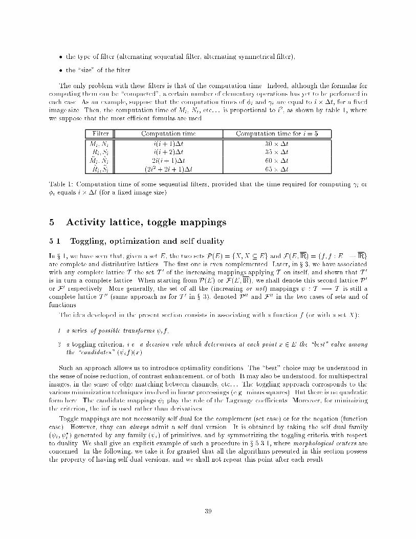
� the type of �lter (alternating sequential �lter, alternating symmetrical �lter),

� the \size" of the �lter.

The only problem with these �lters is that of the computation time. Indeed, although the formulas forcomputing them can be \compacted", a certain number of elementary operations has yet to be performed ineach case. As an example, suppose that the computation times of �i and i are equal to i ��t, for a �xedimage size. Then, the computation time of Mi, Ni, etc: : : is proportional to i2, as shown by table 1, wherewe suppose that the most e�cient fomulas are used.

Filter Computation time Computation time for i = 5

Mi; Ni i(i + 1)�t 30��tRi; Si i(i + 2)�t 35��t~Mi; ~Ni 2i(i+ 1)�t 60��t~Ri; ~Si (2i2 + 2i+ 1)�t 65��t

Table 1: Computation time of some sequential �lters, provided that the time required for computing i or�i equals i ��t (for a �xed image size).

5 Activity lattice, toggle mappings

5.1 Toggling, optimization and self duality

In x 1, we have seen that, given a set E, the two sets P(E) = fX;X � Eg and F(E; IR) = ff; f : E �! IRgare complete and distributive lattices. The �rst one is even complemented. Later, in x 3, we have associatedwith any complete lattice T the set T 0 of the increasing mappings applying T on itself, and shown that T 0is in turn a complete lattice. When starting from P(E) or F(E; IR), we shall denote this second lattice P0or F 0 respectively. More generally, the set of all the (increasing or not) mappings : T �! T is still acomplete lattice T 00 (same approach as for T 0 in x 3), denoted P00 and F 00 in the two cases of sets and offunctions.

The idea developed in the present section consists in associating with a function f (or with a set X):

1. a series of possible transforms if ,

2. a toggling criterion, i.e. a decision rule which determines at each point x 2 E the \best" value amongthe \candidates" ( if)(x).

Such an approach allows us to introduce optimality conditions. The \best" choice may be understood inthe sense of noise reduction, of contrast enhancement, or of both. It may also be understood, for multispectralimages, in the sense of edge matching between channels, etc: : : The toggling approach corresponds to thevarious minimization techniques involved in linear processings (e.g. minus squares). But there is no quadraticform here. The candidate mappings i play the role of the Lagrange coe�cients. Moreover, for minimizingthe criterion, the inf is used rather than derivatives.

Toggle mappings are not necessarily self dual for the complement (set case) or for the negation (functioncase). However, thay can always admit a self dual version. It is obtained by taking the self dual family( i;

�i ) generated by any family ( i) of primitives, and by symmetrizing the toggling criteria with respect

to duality. We shall give an explicit example of such a procedure in x 5.3.1, where morphological centers areconcerned. In the following, we take it for granted that all the algorithms presented in this section possessthe property of having self dual versions, and we shall not repeat this point after each result.

39

5.2 Activity lattice and semi-lattice

5.2.1 Boolean case

Let P(E) be a boolean lattice, and P0, P00 be the two associated operator lattices. Equip P00 with thefollowing relationships:

8 1; 2 2 P 00; 1 � 2 ()�I \ 1 � I \ 2;I [ 1 � I [ 2:

(70)

Note that the second inequality may be rewritten

� \ �1 � � \ �2;with � standing for the complement operator, i.e. � : X 7�! XC .)

Obviously, relation � is an ordering relationship. Moreover, it makes P00 a complete lattice. Indeed, anyminorant m of a family ( i) in P00 satis�es the following system:�

I \m � I \ �;I [m � I [ �; (71)

with� =

[i

i and � =\i

i: (72)

Therefore, if there exists a mapping � verifying�I \ � = I \ �I [ � = I [ �; (73)

then � is larger, for order relation �, than any minorant m. Note that we can modify the second equalityof (73) by using again the complement operator �:

I [ � = I [ � () � \ � = � \ �:

Now, system (73) admits one and one only solution, since every element � 2 P00 may be decomposedinto:

� = (I [�) \ � = (I \ �) [ (� \ �): (74)

By applying this remarkable identity to �, we �nd:

� = (I \ �) [ (� \ �)= [(I \ �) [ �] \ [(I \ �) [�]

=) _ i = � = (I [ �) \ � = (I \ �) [ �; (75)

a quantity which satis�es system (73) (Note that in the present section, _ denotes the inf associated withthe order relation � of lattices P00 or F 00. It is called the activity inf. In the following, __ will also denote theactivity sup.). Similarly, if there exists a smaller majorant � to the family ( i), it must satisfy the system:�

I \ � = I \ �;I [ � = I [ � () � \ � = � \ �: (76)

By using again identity (74), we �nd this time:

__ i = � = (� [ �) \ � = (� \ �) [ �: (77)

Therefore, we have a lattice, which turns out to be complete and distributive (easy proof). We go fromthe inf _ to the sup __ by replacing the identity I by the complementation �. As a matter of fact, the twooperators I and � are just the null element and the universal element of the lattice generated by order �.

40

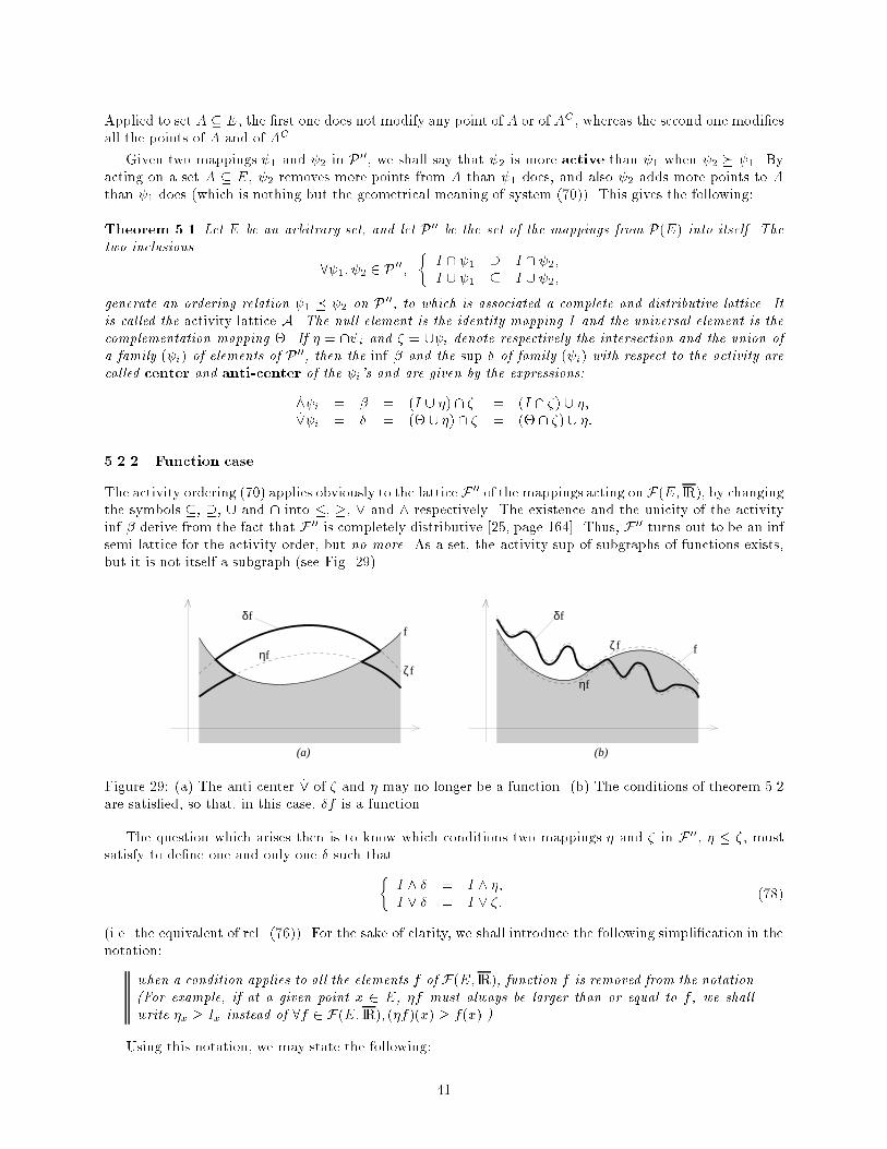
Applied to set A � E, the �rst one does not modify any point of A or of AC , whereas the second one modi�esall the points of A and of AC .

Given two mappings 1 and 2 in P00, we shall say that 2 is more active than 1 when 2 � 1. Byacting on a set A � E, 2 removes more points from A than 1 does, and also 2 adds more points to Athan 1 does (which is nothing but the geometrical meaning of system (70)). This gives the following:

Theorem 5.1 Let E be an arbitrary set, and let P00 be the set of the mappings from P(E) into itself. Thetwo inclusions

8 1; 2 2 P 00;�I \ 1 � I \ 2;I [ 1 � I [ 2;

generate an ordering relation 1 � 2 on P00, to which is associated a complete and distributive lattice. Itis called the activity lattice A. The null element is the identity mapping I and the universal element is thecomplementation mapping �. If � = \ i and � = [ i denote respectively the intersection and the union ofa family ( i) of elements of P00, then the inf � and the sup � of family ( i) with respect to the activity arecalled center and anti-center of the i's and are given by the expressions:

_ i = � = (I [ �) \ � = (I \ �) [ �;__ i = � = (� [ �) \ � = (� \ �) [ �:

5.2.2 Function case

The activity ordering (70) applies obviously to the lattice F 00 of the mappings acting onF(E; IR), by changingthe symbols �, �, [ and \ into �, �, _ and ^ respectively. The existence and the unicity of the activityinf � derive from the fact that F 00 is completely distributive [25, page 164]. Thus, F 00 turns out to be an infsemi-lattice for the activity order, but no more. As a set, the activity sup of subgraphs of functions exists,but it is not itself a subgraph (see Fig. 29).

(a)

f

ζfηf

δf

(b)

δf

ζf

ηf

f

Figure 29: (a) The anti-center __ of � and � may no longer be a function. (b) The conditions of theorem 5.2are satis�ed, so that, in this case, �f is a function.

The question which arises then is to know which conditions two mappings � and � in F 00, � � �, mustsatisfy to de�ne one and only one � such that�

I ^ � = I ^ �;I _ � = I _ �: (78)

(i.e. the equivalent of rel. (76)). For the sake of clarity, we shall introduce the following simpli�cation in thenotation:

when a condition applies to all the elements f of F(E; IR), function f is removed from the notation(For example, if at a given point x 2 E, �f must always be larger than or equal to f , we shallwrite �x � Ix instead of 8f 2 F(E; IR); (�f)(x) � f(x).).

Using this notation, we may state the following:

41

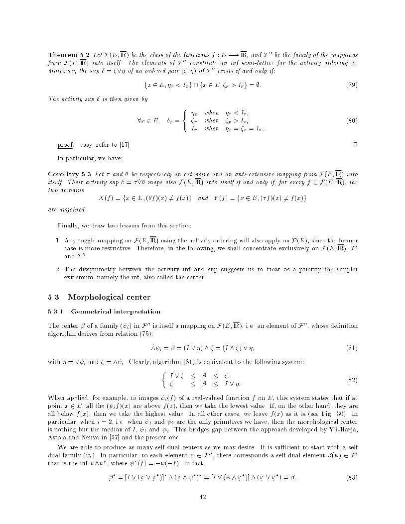
Theorem 5.2 Let F(E; IR) be the class of the functions f : E �! IR, and F 00 be the family of the mappingsfrom F(E; IR) into itself. The elements of F 00 constitute an inf semi-lattice for the activity ordering �.Moreover, the sup � = � __� of an ordered pair (�; �) of F 00 exists if and only if:

fx 2 E; �x < Ixg \ fx 2 E; �x > Ixg = ;: (79)

The activity sup � is then given by

8x 2 E; �x =

8<:

�x when �x < Ix;�x when �x > Ix;Ix when �x = �x = Ix:

(80)

proof: easy, refer to [17]. 2

In particular, we have:

Corollary 5.3 Let � and � be respectively an extensive and an anti-extensive mapping from F(E; IR) intoitself. Their activity sup � = � __� maps also F(E; IR) into itself if and only if, for every f 2 F(E; IR), thetwo domains

X(f) = fx 2 E; (�f)(x) 6= f(x)g and Y (f) = fx 2 E; (�f)(x) 6= f(x)gare disjoined.

Finally, we draw two lessons from this section:

1. Any toggle mapping on F(E; IR) using the activity ordering will also apply on P(E), since the formercase is more restrictive. Therefore, in the following, we shall concentrate exclusively on F(E; IR), F 0and F 00.

2. The dissymmetry between the activity inf and sup suggests us to treat as a priority the simplerextremum, namely the inf, also called the center.

5.3 Morphological center

5.3.1 Geometrical interpretation

The center � of a family ( i) in F 00 is itself a mapping on F(E; IR), i.e. an element of F 00, whose de�nitionalgorithm derives from relation (75):

_ i = � = (I _ �) ^ � = (I ^ �) _ �; (81)

with � = _ i and � = ^ i. Clearly, algorithm (81) is equivalent to the following system:�I _ � � � � �;� � � � I _ �: (82)

When applied, for example, to images i(f) of a real-valued function f on E, this system states that if atpoint x 2 E, all the ( if)(x) are above f(x), then we take the lowest value. If, on the other hand, they areall below f(x), then we take the highest value. In all other cases, we leave f(x) as it is (see Fig. 30). Inparticular, when i = 2, i.e. when 1 and 2 are the only primitives we have, then the morphological centeris nothing but the median of I, 1 and 2. This bridges gap between the approach developed by Yli-Harja,Astola and Neuvo in [37] and the present one.

We are able to produce as many self dual centers as we may desire. It is su�cient to start with a selfdual family ( i). In particular, to each element 2 F 00, there corresponds a self-dual element �( ) 2 F 0that is the inf _ �, where �(f) = � (�f). In fact,

�� = [I _ ( _ �)]� ^ ( ^ �)� = [I _ ( ^ �)] ^ ( _ �) = �: (83)

42

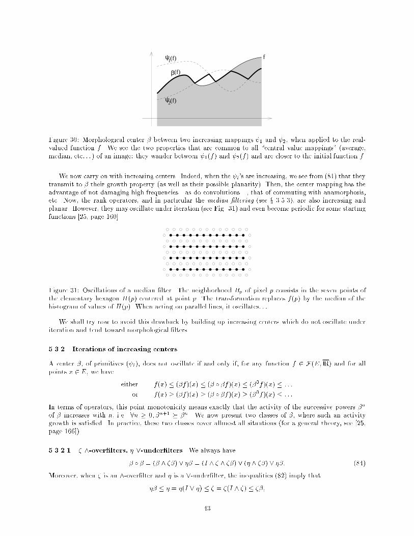
f

β

ψ1

ψ2

(f)

(f)

(f)

Figure 30: Morphological center � between two increasing mappings 1 and 2, when applied to the real-valued function f . We see the two properties that are common to all \central value mappings" (average,median, etc: : : ) of an image: they wander between 1(f) and 2(f) and are closer to the initial function f .

We now carry on with increasing centers. Indeed, when the i's are increasing, we see from (81) that theytransmit to � their growth property (as well as their possible planarity). Then, the center mapping has theadvantage of not damaging high frequencies|as do convolutions|, that of commuting with anamorphosis,etc. Now, the rank operators, and in particular the median �ltering (see x 3.5.3), are also increasing andplanar. However, they may oscillate under iteration (see Fig. 31) and even become periodic for some startingfunctions [25, page 160].

Figure 31: Oscillations of a median �lter. The neighborhood Bp of pixel p consists in the seven points ofthe elementary hexagon H(p) centered at point p. The transformation replaces f(p) by the median of thehistogram of values of H(p). When acting on parallel lines, it oscillates: : :

We shall try now to avoid this drawback by building up increasing centers which do not oscillate underiteration and tend toward morphological �lters.

5.3.2 Iterations of increasing centers

A center �, of primitives ( i), does not oscillate if and only if, for any function f 2 F(E; IR) and for allpoints x 2 E, we have

either f(x) � (�f)(x) � (� � �f)(x) � (�3f)(x) � : : :

or f(x) � (�f)(x) � (� � �f)(x) � (�3f)(x) � : : :

In terms of operators, this point monotonicity means exactly that the activity of the successive powers �n

of � increases with n, i.e. 8n � 0; �n+1 � �n. We now present two classes of �, where such an activitygrowth is satis�ed. In practice, these two classes cover allmost all situations (for a general theory, see [25,page 166]).

5.3.2.1 � ^-over�lters, � _-under�lters We always have

� � � = (� ^ ��) _ �� = (I ^ � ^ ��) _ (� ^ ��) _ ��: (84)

Moreover, when � is an ^-over�lter and � is a _-under�lter, the inequalities (82) imply that

�� � � = �(I _ �) � � = �(I ^ �) � ��;

43

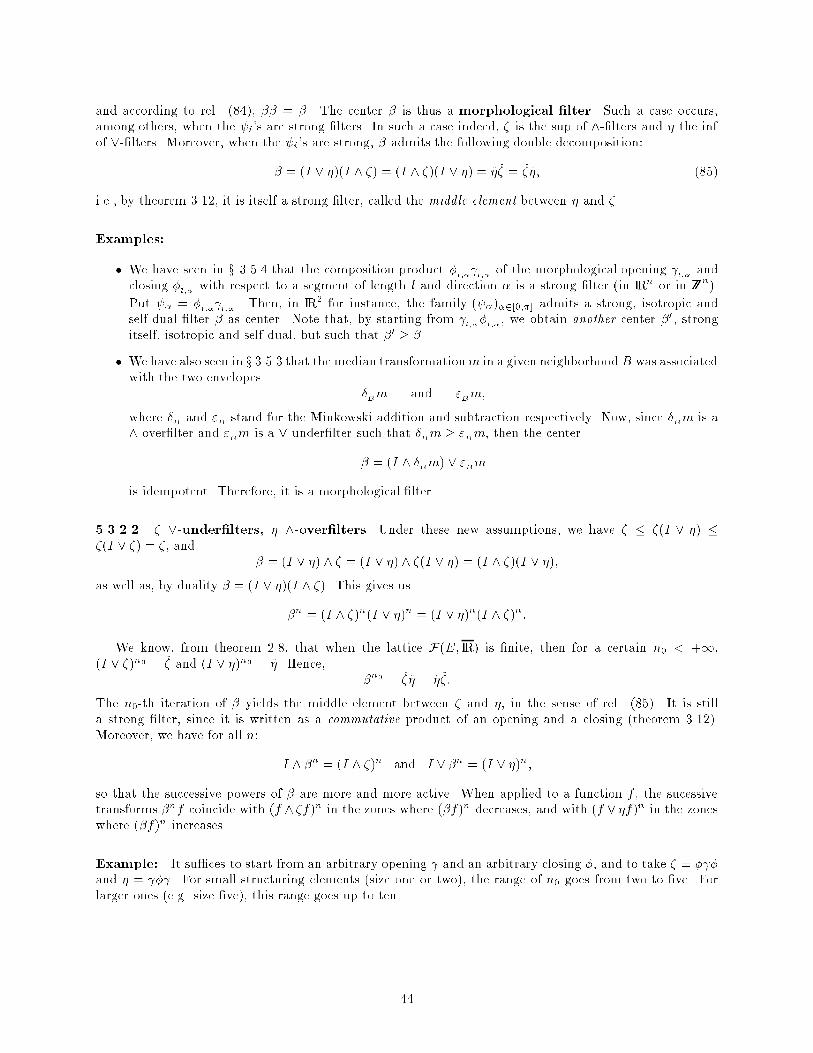
and according to rel. (84), �� = �. The center � is thus a morphological �lter. Such a case occurs,among others, when the i's are strong �lters. In such a case indeed, � is the sup of ^-�lters and � the infof _-�lters. Moreover, when the i's are strong, � admits the following double decomposition:

� = (I _ �)(I ^ �) = (I ^ �)(I _ �) = ��� = ���; (85)

i.e., by theorem 3.12, it is itself a strong �lter, called the middle element between � and �.

Examples:

� We have seen in x 3.5.4 that the composition product �l;� l;�

of the morphological opening l;�

andclosing �

l;�with respect to a segment of length l and direction � is a strong �lter (in IRn or in ZZ

n).

Put � = �l;� l;�. Then, in IR2 for instance, the family ( �)�2[0;�] admits a strong, isotropic and

self-dual �lter � as center. Note that, by starting from l;��l;�, we obtain another center �0, strong

itself, isotropic and self-dual, but such that �0 � �.

� We have also seen in x 3.5.3 that the median transformationm in a given neighborhood B was associatedwith the two envelopes

�Bm and "

Bm;

where �Band "

Bstand for the Minkowski addition and subtraction respectively. Now, since �

Bm is a

^-over�lter and "Bm is a _-under�lter such that �

Bm � "

Bm, then the center

� = (I ^ �Bm) _ "

Bm

is idempotent. Therefore, it is a morphological �lter.

5.3.2.2 � _-under�lters, � ^-over�lters Under these new assumptions, we have � � �(I _ �) ��(I _ �) = �, and

� = (I _ �) ^ � = (I _ �) ^ �(I _ �) = (I ^ �)(I _ �);as well as, by duality � = (I _ �)(I ^ �). This gives us

�n = (I ^ �)n(I _ �)n = (I _ �)n(I ^ �)n:

We know, from theorem 2.8, that when the lattice F(E; IR) is �nite, then for a certain n0 < +1,(I _ �)n0 = �� and (I _ �)n0 = �. Hence,

�n0 = ��� = ���:

The n0-th iteration of � yields the middle element between � and �, in the sense of rel. (85). It is stilla strong �lter, since it is written as a commutative product of an opening and a closing (theorem 3.12).Moreover, we have for all n:

I ^ �n = (I ^ �)n and I _ �n = (I _ �)n;

so that the successive powers of � are more and more active. When applied to a function f , the sucessivetransforms �nf coincide with (f ^ �f)n in the zones where (�f)n decreases, and with (f _ �f)n in the zoneswhere (�f)n increases.

Example: It su�ces to start from an arbitrary opening and an arbitrary closing �, and to take � = � �and � = � . For small structuring elements (size one or two), the range of n0 goes from two to �ve. Forlarger ones (e.g. size �ve), this range goes up to ten.

44

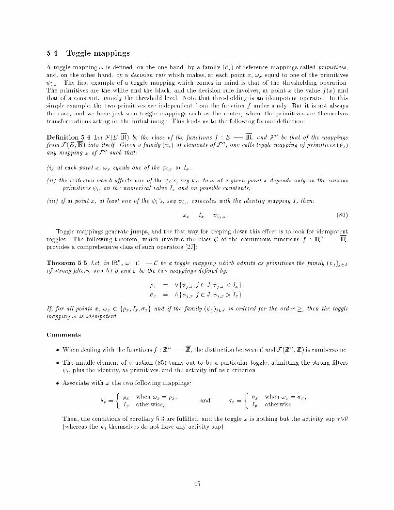
5.4 Toggle mappings

A toggle mapping ! is de�ned, on the one hand, by a family (�i) of reference mappings called primitives,and, on the other hand, by a decision rule which makes, at each point x, !x equal to one of the primitives i;x. The �rst example of a toggle mapping which comes in mind is that of the thresholding operation.The primitives are the white and the black, and the decision rule involves, at point x the value f(x) andthat of a constant, namely the threshold level. Note that thresholding is an idempotent operator. In thissimple example, the two primitives are independent from the function f under study. But it is not alwaysthe case, and we have just seen toggle mappings such as the center, where the primitives are themselvestransformations acting on the initial image. This leads us to the following formal de�nition:

De�nition 5.4 Let F(E; IR) be the class of the functions f : E �! IR, and F 00 be that of the mappingsfrom F(E; IR) into itself. Given a family ( i) of elements of F 00, one calls toggle mapping of primitives ( i)any mapping ! of F 00 such that:

(i) at each point x, !x equals one of the i;x or Ix,

(ii) the criterion which a�ects one of the i's, say i0 to ! at a given point x depends only on the variousprimitives i, on the numerical value Ix and on possible constants,

(iii) if at point x, at least one of the i's, say i0 , coincides with the identity mapping I, then:

!x = Ix = i0;x: (86)

Toggle mappings generate jumps, and the �rst way for keeping down this e�ect is to look for idempotenttoggles. The following theorem, which involves the class C of the continuous functions f : IRn �! IR,provides a comprehensive class of such operators [27]:

Theorem 5.5 Let, in IRn, ! : C �! C be a toggle mapping which admits as primitives the family ( j)j2Jof strong �lters, and let � and � be the two mappings de�ned by:

�x = _f j;x; j 2 J; j;x < Ixg;�x = ^f j;x; j 2 J; j;x > Ixg:

If, for all points x, !x 2 f�x; Ix; �xg and if the family ( j)j2J is ordered for the order �, then the togglemapping ! is idempotent.

Comments

� When dealing with the functions f : ZZn �! ZZ, the distinction between C andF(ZZn;ZZ) is cumbersome.

� The middle element of equation (85) turns out to be a particular toggle, admitting the strong �lters i, plus the identity, as primitives, and the activity inf as a criterion.

� Associate with ! the two following mappings:

�x =

��x when !x = �x,Ix otherwise,

and �x =

��x when !x = �x,Ix otherwise.

Then, the conditions of corollary 5.3 are ful�lled, and the toggle ! is nothing but the activity sup � __�(whereas the i themselves do not have any activity sup).

45

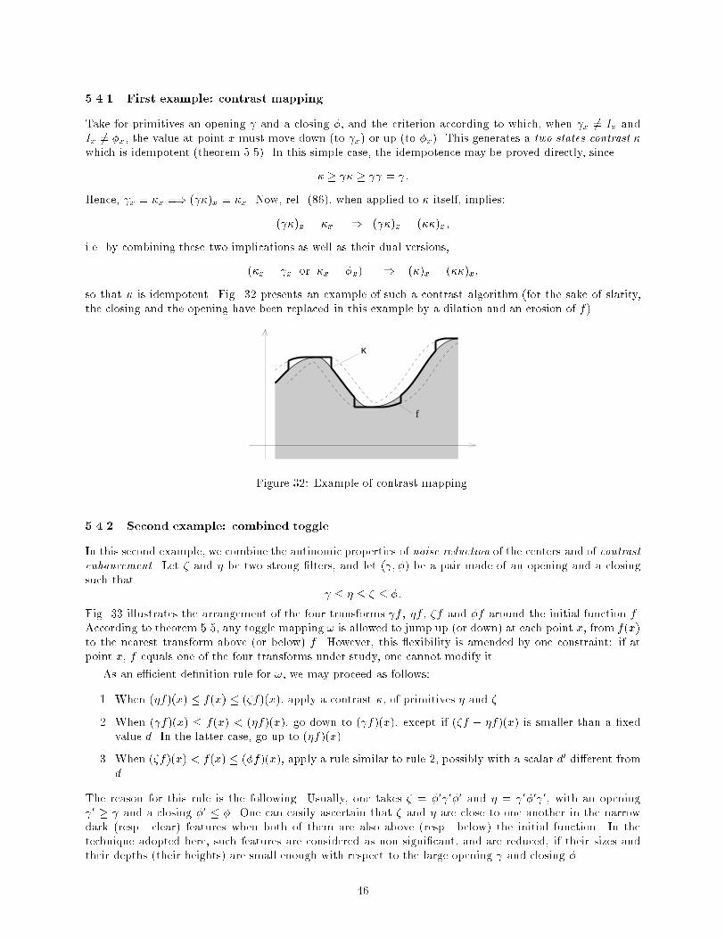
5.4.1 First example: contrast mapping

Take for primitives an opening and a closing �, and the criterion according to which, when x 6= Ix andIx 6= �x, the value at point x must move down (to x) or up (to �x). This generates a two states contrast �which is idempotent (theorem 5.5). In this simple case, the idempotence may be proved directly, since

� � � � = :

Hence, x = �x =) ( �)x = �x. Now, rel. (86), when applied to � itself, implies:

( �)x = �x =) ( �)x = (��)x;

i.e. by combining these two implications as well as their dual versions,

(�x = x or �x = �x) =) (�)x = (��)x;

so that � is idempotent. Fig. 32 presents an example of such a contrast algorithm (for the sake of slarity,the closing and the opening have been replaced in this example by a dilation and an erosion of f).

f

κ

Figure 32: Example of contrast mapping.

5.4.2 Second example: combined toggle

In this second example, we combine the antinomic properties of noise reduction of the centers and of contrastenhancement. Let � and � be two strong �lters, and let ( ; �) be a pair made of an opening and a closingsuch that

� � � � � �:

Fig. 33 illustrates the arrangement of the four transforms f , �f , �f and �f around the initial function f .According to theorem 5.5, any toggle mapping ! is allowed to jump up (or down) at each point x, from f(x)to the nearest transform above (or below) f . However, this exibility is amended by one constraint: if atpoint x, f equals one of the four transforms under study, one cannot modify it.

As an e�cient de�nition rule for !, we may proceed as follows:

1. When (�f)(x) � f(x) � (�f)(x), apply a contrast �, of primitives � and �.

2. When ( f)(x) � f(x) < (�f)(x), go down to ( f)(x), except if (�f � �f)(x) is smaller than a �xedvalue d. In the latter case, go up to (�f)(x).

3. When (�f)(x) < f(x) � (�f)(x), apply a rule similar to rule 2, possibly with a scalar d0 di�erent fromd.

The reason for this rule is the following. Usually, one takes � = �0 0�0 and � = 0�0 0, with an opening 0 � and a closing �0 � �. One can easily ascertain that � and � are close to one another in the narrowdark (resp. clear) features when both of them are also above (resp. below) the initial function. In thetechnique adopted here, such features are considered as non signi�cant, and are reduced, if their sizes andtheir depths (their heights) are small enough with respect to the large opening and closing �.

46

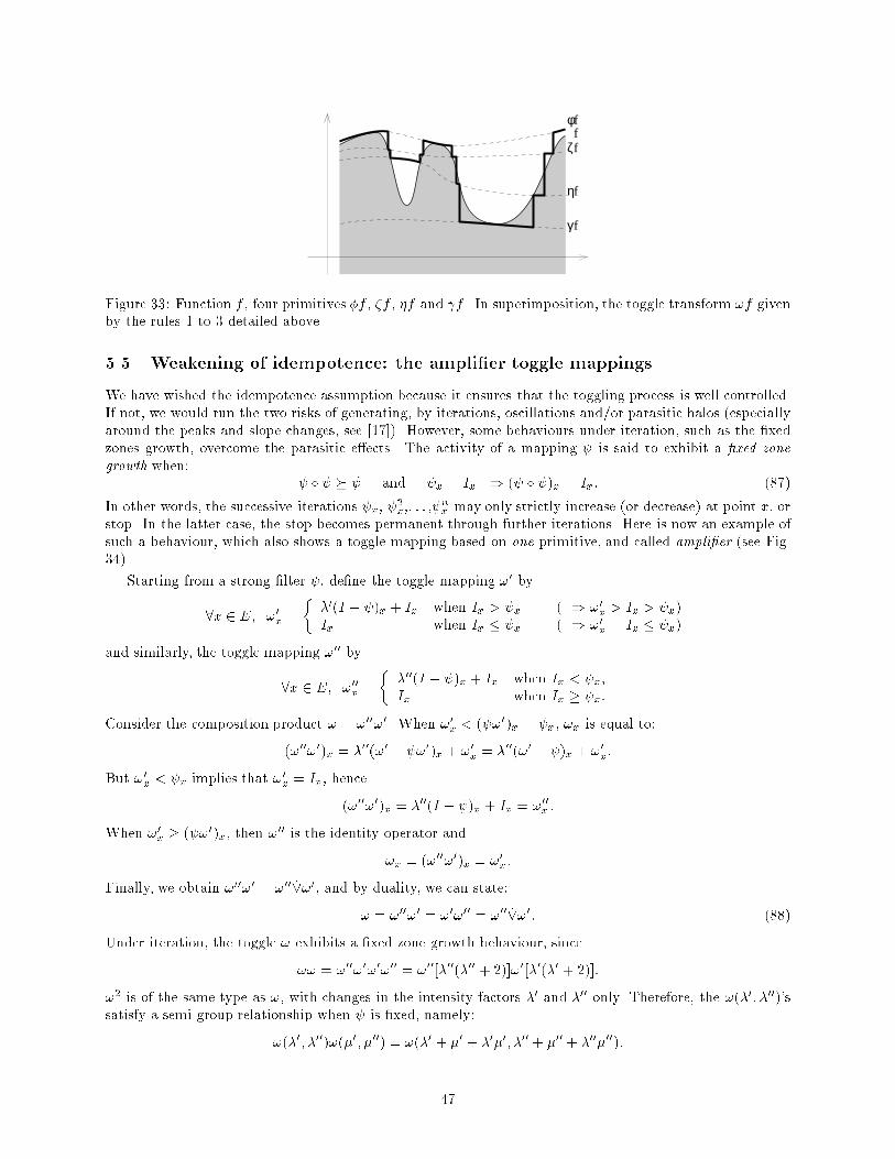
φf

ζf

ηf

γf

f

Figure 33: Function f , four primitives �f , �f , �f and f . In superimposition, the toggle transform !f givenby the rules 1 to 3 detailed above.

5.5 Weakening of idempotence: the ampli�er toggle mappings

We have wished the idempotence assumption because it ensures that the toggling process is well controlled.If not, we would run the two risks of generating, by iterations, oscillations and/or parasitic halos (especiallyaround the peaks and slope changes, see [17]). However, some behaviours under iteration, such as the �xedzones growth, overcome the parasitic e�ects. The activity of a mapping is said to exhibit a �xed zonegrowth when:

� � and x = Ix =) ( � )x = Ix: (87)

In other words, the successive iterations x, 2x,: : : ,

nx may only strictly increase (or decrease) at point x, or

stop. In the latter case, the stop becomes permanent through further iterations. Here is now an example ofsuch a behaviour, which also shows a toggle mapping based on one primitive, and called ampli�er (see Fig.34).

Starting from a strong �lter , de�ne the toggle mapping !0 by

8x 2 E; !0x =

��0(I � )x + Ix when Ix > x (=) !0x > Ix > x)Ix when Ix � x (=) !0x = Ix � x)

and similarly, the toggle mapping !00 by

8x 2 E; !00x =

��00(I � )x + Ix when Ix < x;Ix when Ix � x:

Consider the composition product ! = !00!0. When !0x < ( !0)x = x, !x is equal to:

(!00!0)x = �00(!0 � !0)x + !0x = �00(!0 � )x + !0x:

But !0x < x implies that !0x = Ix, hence

(!00!0)x = �00(I � )x + Ix = !00x :

When !0x � ( !0)x, then !00 is the identity operator and

!x = (!00!0)x = !0x:

Finally, we obtain !00!0 = !00 __!0, and by duality, we can state:

! = !00!0 = !0!00 = !00 __!0: (88)

Under iteration, the toggle ! exhibits a �xed zone growth behaviour, since

!! = !00!0!0!00 = !00[�00(�00 + 2)]!0[�0(�0 + 2)]:

!2 is of the same type as !, with changes in the intensity factors �0 and �00 only. Therefore, the !(�0; �00)'ssatisfy a semi-group relationship when is �xed, namely:

!(�0; �00)!(�0; �00) = !(�0 + �0 + �0�0; �00 + �00 + �00�00):

47

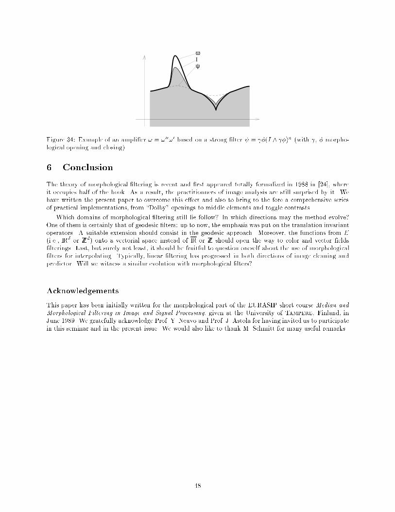
ωIψ

Figure 34: Example of an ampli�er ! = !00!0 based on a strong �lter = �(I ^ �)n (with , � morpho-logical opening and closing).

6 Conclusion

The theory of morphological �ltering is recent and �rst appeared totally formalized in 1988 in [24], whereit occupies half of the book. As a result, the practitionners of image analysis are still surprised by it. Wehave written the present paper to overcome this e�ect and also to bring to the fore a comprehensive seriesof practical implementations, from \Dolby" openings to middle elements and toggle contrasts.

Which domains of morphological �ltering still lie follow? In which directions may the method evolve?One of them is certainly that of geodesic �lters: up to now, the emphasis was put on the translation invariantoperators. A suitable extension should consist in the geodesic approach. Moreover, the functions from E(i.e., IRd or ZZd) onto a vectorial space instead of IR or ZZ should open the way to color and vector �elds�lterings. Last, but surely not least, it should be fruitful to question oneself about the use of morphological�lters for interpolating. Typically, linear �ltering has progressed in both directions of image cleaning andpredictor. Will we witness a similar evolution with morphological �lters?

Acknowledgements

This paper has been initially written for the morphological part of the EURASIP short course Median andMorphological Filtering in Image and Signal Processing, given at the University of Tampere, Finland, inJune 1989. We gratefully acknowledge Prof. Y. Neuvo and Prof. J. Astola for having invited us to participatein this seminar and in the present issue. We would also like to thank M. Schmitt for many useful remarks.

48

References

[1] S. Beucher. Segmentation d'Images et Morphologie Math�ematique. PhD thesis, Ecole des Mines, Paris,June 1990.

[2] S. Beucher and C. Lantu�ejoul. Use of watersheds in contour detection. In International Workshop onImage Processing, Real-Time Edge and Motion Detection/Estimation, Rennes, France, 1979.

[3] S. Beucher and L. Vincent. Introduction aux outils morphologiques de segmentation. In Traitementd'Images en Microscopie �a Balayage et en Microanalyse par Sonde Electronique, pages F41{F43. ANRT,Paris, Mar. 1990.

[4] G. Birkho�. Lattice Theory, volume 25. A.M.S. Colloq., third edition, 1983.

[5] H. Heijmans. Mophological �ltering and iteration. In SPIE Vol. 1360, Visual Communications andImage Processing, pages 166{175, Lausanne, Switzerland, Oct. 1990.

[6] H. Heijmans and C. Ronse. The algebraic basis of mathematical morphology. part I: Dilations anderosions. Comp. Vis., Graphics and Image Processing, 50:245{295, 1990.

[7] H. Heijmans and J. Serra. Convergence, continuity and iteration in mathematicalmorphology. TechnicalReport BS-R-9104, Centre for Mathematics and Computer Science, Amsterdam, 1991.

[8] G. Heygster. Rank �lters in digital image processing. Comp. Graphics and Image Processing, 19(2):148{164, June 1982.

[9] B. Kurdy and D. Jeulin. Directional mathematical morphology operations. In 5th European CongressFor Stereology, pages 473{480, Freiburg im Breisgau FRG, Sept. 1989. Acta Stereologica. Vol. 8/2.

[10] C. Lantu�ejoul and S. Beucher. On the use of the geodesic metric in image analysis. Journal of Microscopy,121:39{49, Jan. 1981.

[11] R. Lougheed. Lecture notes for summer course on mathematical morphology. Technical report, Univer-sity of Michigan, 1983.

[12] P. Maragos and R. Schafer. Morphological �lters|part i: their set-theoretic analysis and relations tolinear shift-invariant �lters. IEEE Trans. on Acoustics, Speech and Signal Processing, 35(8):1153{1169,Aug. 1987.

[13] P. Maragos and R. Schafer. Morphological �lters|part ii: their relations to median, order-statistics,and stack �lters. IEEE Trans. on Acoustics, Speech and Signal Processing, 35(8):1170{1184, Aug. 1987.

[14] G. Matheron. El�ements pour une Th�eorie des Milieux Poreux. Masson, Paris, 1967.

[15] G. Matheron. Random Sets and Integral Geometry. John Wiley and Sons, New York, 1975.

[16] F. Meyer. Contrast feature extraction. In J.-L. Chermant, editor, Quantitative Analysis of Microstruc-tures in Material Sciences, Biology and Medicine, Stuttgart, FRG, 1978. Riederer Verlag. Special issueof Practical Metallography.

[17] F. Meyer and J. Serra. Contrasts and activity lattice. Signal Processing, 16(4):303{317, Apr. 1989.

[18] F. Meyer and J. Serra. Filters: from theory to practice. In 5th European Congress For Stereology, pages503{508, Freiburg im Breisgau FRG, Sept. 1989. Acta Stereologica. Vol. 8/2.

[19] K. Preston and M. Du�. Modern Cellular Automata. Plenum, New York, 1985.

[20] C. Ronse. Erosion of narrow image features by combining local rank and max �lters. In SecondInternational Conference on Image Processing and its Applications, pages 77{81, London, 1986.

49

[21] C. Ronse and H. Heijmans. The algebraic basis of mathematical morphology. part II: Openings andclosings. Comp. Vis., Graph, and Im. Proc.: Image Understanding, 54:74{97, 1991.

[22] A. Rosenfeld and A. Kak. Digital Image Processing. Academic Press, New York, 1976.

[23] J. Serra. Morphologie pour les fonctions \�a peu pr�es en tout ou rien". Technical report, Ecole desMines, Paris, Apr. 1975.

[24] J. Serra. Image Analysis and Mathematical Morphology. Academic Press, London, 1982.

[25] J. Serra, editor. Image Analysis and Mathematical Morphology, Volume 2: Theoretical Advances. Aca-demic Press, London, 1988.

[26] J. Serra. It�erations et convergence. Technical report, Ecole des Mines, CMM, Paris, Feb. 1989.

[27] J. Serra. Toggle mappings. In J.-C. Simon, editor, From Pixels to Features, pages 61{72. North Holland,Amsterdam, 1989.

[28] J. Serra and L. Vincent. Lecture notes on morphological �ltering. Cahiers du Centre de MorphologieMath�ematique 8, Ecole des Mines, CMM, Paris, 1989.

[29] S. R. Sternberg. Parallel architecture for image processing. In 3rd Int. IEEE Compsac, Chicago, 1979.

[30] S. R. Sternberg. Grayscale morphology. Comp. Vis., Graphics and Image Processing, 35:333{355, 1986.

[31] L. Vincent. Graphs and mathematical morphology. Signal Processing, 16:365{388, Apr. 1989.

[32] L. Vincent. Mathematical morphology for graphs applied to image description and segmentation. InElectronic Imaging West 89, pages Vol. 1, pp. 313{318, Pasadena, CA, 1989.

[33] L. Vincent. Algorithmes Morphologiques �a Base de Files d'Attente et de Lacets: Extension aux Graphes.PhD thesis, Ecole des Mines, Paris, May 1990.

[34] L. Vincent and P. Soille. Watersheds in digital spaces: an e�cient algorithm based on immersionsimulations. IEEE Trans. Pattern Anal. Machine Intell., 13(6):583{598, June 1991.

[35] J. Vitria. Estudi Sobre L'Automatitzacio de l'Analisi Visual de Circuits Integrats Mitjan�cant MorfologiaMatematica. PhD thesis, Universitat Autonoma de Barcelona, Barcelona, Oct. 1990.

[36] P. Wendt, E. Coyle, and N. Gallagher. Stack �lters. IEEE Transactions on Acoustics Speech and SignalProcessing, 34(4):898{911, Aug. 1986.

[37] O. Yli-Harja, J. Astola, and Y. Neuvo. Analysis of the properties of median and weighted median �ltersusing threshold logic and stack �lter representation. IEEE Transactions on Acoustics Speech and SignalProcessing, 1989. (submitted).

50

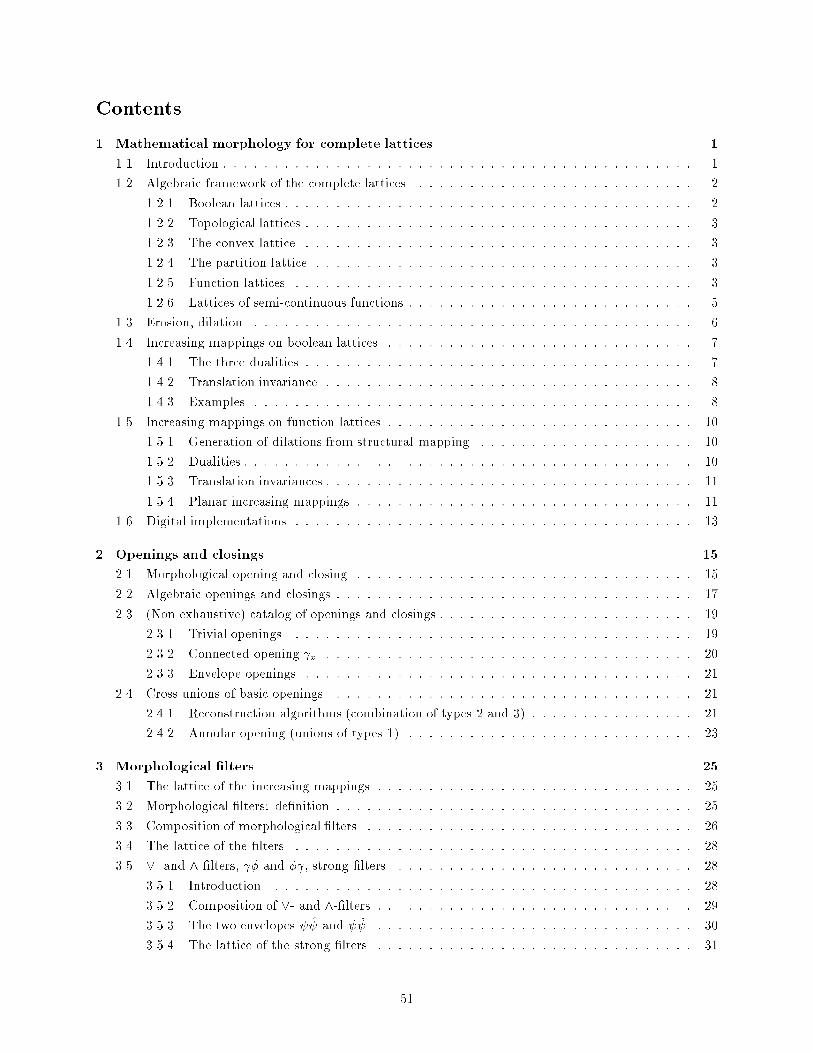
Contents

1 Mathematical morphology for complete lattices 1

1.1 Introduction : : : : : : : : : : : : : : : : : : : : : : : : : : : : : : : : : : : : : : : : : : : : : : 1

1.2 Algebraic framework of the complete lattices : : : : : : : : : : : : : : : : : : : : : : : : : : : 2

1.2.1 Boolean lattices : : : : : : : : : : : : : : : : : : : : : : : : : : : : : : : : : : : : : : : : 2

1.2.2 Topological lattices : : : : : : : : : : : : : : : : : : : : : : : : : : : : : : : : : : : : : : 3

1.2.3 The convex lattice : : : : : : : : : : : : : : : : : : : : : : : : : : : : : : : : : : : : : : 3

1.2.4 The partition lattice : : : : : : : : : : : : : : : : : : : : : : : : : : : : : : : : : : : : : 3

1.2.5 Function lattices : : : : : : : : : : : : : : : : : : : : : : : : : : : : : : : : : : : : : : : 3

1.2.6 Lattices of semi-continuous functions : : : : : : : : : : : : : : : : : : : : : : : : : : : : 5

1.3 Erosion, dilation : : : : : : : : : : : : : : : : : : : : : : : : : : : : : : : : : : : : : : : : : : : 6

1.4 Increasing mappings on boolean lattices : : : : : : : : : : : : : : : : : : : : : : : : : : : : : : 7

1.4.1 The three dualities : : : : : : : : : : : : : : : : : : : : : : : : : : : : : : : : : : : : : : 7

1.4.2 Translation invariance : : : : : : : : : : : : : : : : : : : : : : : : : : : : : : : : : : : : 8

1.4.3 Examples : : : : : : : : : : : : : : : : : : : : : : : : : : : : : : : : : : : : : : : : : : : 8

1.5 Increasing mappings on function lattices : : : : : : : : : : : : : : : : : : : : : : : : : : : : : : 10

1.5.1 Generation of dilations from structural mapping : : : : : : : : : : : : : : : : : : : : : 10

1.5.2 Dualities : : : : : : : : : : : : : : : : : : : : : : : : : : : : : : : : : : : : : : : : : : : : 10

1.5.3 Translation invariances : : : : : : : : : : : : : : : : : : : : : : : : : : : : : : : : : : : : 11

1.5.4 Planar increasing mappings : : : : : : : : : : : : : : : : : : : : : : : : : : : : : : : : : 11

1.6 Digital implementations : : : : : : : : : : : : : : : : : : : : : : : : : : : : : : : : : : : : : : : 13

2 Openings and closings 15

2.1 Morphological opening and closing : : : : : : : : : : : : : : : : : : : : : : : : : : : : : : : : : 15

2.2 Algebraic openings and closings : : : : : : : : : : : : : : : : : : : : : : : : : : : : : : : : : : : 17

2.3 (Non exhaustive) catalog of openings and closings : : : : : : : : : : : : : : : : : : : : : : : : : 19

2.3.1 Trivial openings : : : : : : : : : : : : : : : : : : : : : : : : : : : : : : : : : : : : : : : 19

2.3.2 Connected opening x : : : : : : : : : : : : : : : : : : : : : : : : : : : : : : : : : : : : 20

2.3.3 Envelope openings : : : : : : : : : : : : : : : : : : : : : : : : : : : : : : : : : : : : : : 21

2.4 Cross-unions of basic openings : : : : : : : : : : : : : : : : : : : : : : : : : : : : : : : : : : : 21

2.4.1 Reconstruction algorithms (combination of types 2 and 3) : : : : : : : : : : : : : : : : 21

2.4.2 Annular opening (unions of types 1) : : : : : : : : : : : : : : : : : : : : : : : : : : : : 23

3 Morphological �lters 25

3.1 The lattice of the increasing mappings : : : : : : : : : : : : : : : : : : : : : : : : : : : : : : : 25

3.2 Morphological �lters: de�nition : : : : : : : : : : : : : : : : : : : : : : : : : : : : : : : : : : : 25

3.3 Composition of morphological �lters : : : : : : : : : : : : : : : : : : : : : : : : : : : : : : : : 26

3.4 The lattice of the �lters : : : : : : : : : : : : : : : : : : : : : : : : : : : : : : : : : : : : : : : 28

3.5 _- and ^-�lters, � and � , strong �lters : : : : : : : : : : : : : : : : : : : : : : : : : : : : : 28

3.5.1 Introduction : : : : : : : : : : : : : : : : : : : : : : : : : : : : : : : : : : : : : : : : : 28

3.5.2 Composition of _- and ^-�lters : : : : : : : : : : : : : : : : : : : : : : : : : : : : : : : 29

3.5.3 The two envelopes and � : : : : : : : : : : : : : : : : : : : : : : : : : : : : : : : 30

3.5.4 The lattice of the strong �lters : : : : : : : : : : : : : : : : : : : : : : : : : : : : : : : 31

51

3.6 Filtering as a tool for segmentation : : : : : : : : : : : : : : : : : : : : : : : : : : : : : : : : : 32

4 Granulometries, Alternating Sequential Filters 34

4.1 Size distributions : : : : : : : : : : : : : : : : : : : : : : : : : : : : : : : : : : : : : : : : : : : 34

4.2 Alternating Sequential Filters : : : : : : : : : : : : : : : : : : : : : : : : : : : : : : : : : : : : 36

4.2.1 Introduction : : : : : : : : : : : : : : : : : : : : : : : : : : : : : : : : : : : : : : : : : 36

4.2.2 De�nitions : : : : : : : : : : : : : : : : : : : : : : : : : : : : : : : : : : : : : : : : : : 36

4.2.3 Properties : : : : : : : : : : : : : : : : : : : : : : : : : : : : : : : : : : : : : : : : : : : 38

4.2.4 Applications, computation time : : : : : : : : : : : : : : : : : : : : : : : : : : : : : : : 38

5 Activity lattice, toggle mappings 39

5.1 Toggling, optimization and self duality : : : : : : : : : : : : : : : : : : : : : : : : : : : : : : : 39

5.2 Activity lattice and semi-lattice : : : : : : : : : : : : : : : : : : : : : : : : : : : : : : : : : : : 40

5.2.1 Boolean case : : : : : : : : : : : : : : : : : : : : : : : : : : : : : : : : : : : : : : : : : 40

5.2.2 Function case : : : : : : : : : : : : : : : : : : : : : : : : : : : : : : : : : : : : : : : : : 41

5.3 Morphological center : : : : : : : : : : : : : : : : : : : : : : : : : : : : : : : : : : : : : : : : : 42

5.3.1 Geometrical interpretation : : : : : : : : : : : : : : : : : : : : : : : : : : : : : : : : : : 42

5.3.2 Iterations of increasing centers : : : : : : : : : : : : : : : : : : : : : : : : : : : : : : : 43

5.4 Toggle mappings : : : : : : : : : : : : : : : : : : : : : : : : : : : : : : : : : : : : : : : : : : : 45

5.4.1 First example: contrast mapping : : : : : : : : : : : : : : : : : : : : : : : : : : : : : : 46

5.4.2 Second example: combined toggle : : : : : : : : : : : : : : : : : : : : : : : : : : : : : 46

5.5 Weakening of idempotence: the ampli�er toggle mappings : : : : : : : : : : : : : : : : : : : : 47

6 Conclusion 48

52

List of Figures

1 Milestones for the morphological �ltering theory : Moore : a (� 1920) ; Matheron : b, c [14] ;d [15] ; g, h, i, j [25] ; Serra : e, f, j, k [25] ; l [17] ; m [27] ; Sternberg : e [30] ; Meyer :l [17] ; Ronse and Heijmans : o [21] ; speci�ed �lters : rank opening (Ronse [20]), segmentbased �lters (Meyer and Serra [17]) ; orientation dependent �ltering (Kurdy and Jeulin [9]) ;�lters for graphs (Vincent [31]) ; multispectral �ltering (Vitria [35]) ; etc: : : : : : : : : : : : : 1

2 Umbra U+(X) of a set X � IR� IR. : : : : : : : : : : : : : : : : : : : : : : : : : : : : : : : : 4

3 The threshold mapping . : : : : : : : : : : : : : : : : : : : : : : : : : : : : : : : : : : : : : : 4

4 The family of functions (fi). : : : : : : : : : : : : : : : : : : : : : : : : : : : : : : : : : : : : : 5

5 A function without a maximum (it is not u.s.c.). : : : : : : : : : : : : : : : : : : : : : : : : : 6

6 Dilation of a set X by a bipoint �B. : : : : : : : : : : : : : : : : : : : : : : : : : : : : : : : : : 9

7 Erosion of a set X by a segment �S. : : : : : : : : : : : : : : : : : : : : : : : : : : : : : : : : : 9

8 Dilation and erosion of X by a disc D = �D. : : : : : : : : : : : : : : : : : : : : : : : : : : : : 9

9 Comparison between the dilations of X by a disc and by an hexagon. Note that these struc-turing elements are symmetrical: D = �D and H = �H. : : : : : : : : : : : : : : : : : : : : : : 9

10 Successive geodesic dilations of set Y inside set X. : : : : : : : : : : : : : : : : : : : : : : : : 10

11 An example of a planar increasing mapping. : : : : : : : : : : : : : : : : : : : : : : : : : : : : 12

12 Dilation (a) and erosion (b) of a function f by a planar structuring element B. : : : : : : : : 12

13 Basic spherical shapes in ZZ3. The plane z = 0 corresponds to the median horizontal sectionof the cube. The structuring functions derive from these sets by taking their umbrae. : : : : : 14

14 The elementary rhombododecahedron R (i.e. Steiner rhomb of ZZ3) and its decomposition infour dilations by segments. The complex shape of the polyhedron has been decomposed intofour simple structuring functions, whose implementation is very simple and extremely e�cient. 14

15 Dilation of the Steiner rhomb R by R� (R� is obtained in the same way as R, by four dilationsby doublets). : : : : : : : : : : : : : : : : : : : : : : : : : : : : : : : : : : : : : : : : : : : : : 15

16 The elementary cuboctahedron C and its decomposition into two successive horizontal planes. 15

17 Examples of a morphological opening and of a morphological closing of a set X by a disc D. : 16

18 m(X) is the smallest element Y � T such that "(Y ) = "(X). : : : : : : : : : : : : : : : : : : 17

19 Comparison between the openings of a 1-D function by an horizontal segment S and by a discD. : : : : : : : : : : : : : : : : : : : : : : : : : : : : : : : : : : : : : : : : : : : : : : : : : : : 18

20 The opening called the connected component of A that contains point x. : : : : : : : : : : : : 20

21 A less obvious connectivity notion, associated with the opening �x. : : : : : : : : : : : : : : : 20

22 Algebraic opening which is de�ned as a morphological opening by a disc followed by a recon-struction : : : : : : : : : : : : : : : : : : : : : : : : : : : : : : : : : : : : : : : : : : : : : : : : 22

23 Grey-scale reconstruction of function f from the \marker-function" g: the right peak of f ismarked by g and thus preserved in the reconstruction process. : : : : : : : : : : : : : : : : : : 23

24 Annular opening versus a classical opening by a disc and a union of openings by segments. 24

25 An example of a _-�lter (a) and of a strong �lter (b). : : : : : : : : : : : : : : : : : : : : : : 29

26 A case where it is not necessary to perform iterations: the opening l and the closing �l withrespect to a segment l. : : : : : : : : : : : : : : : : : : : : : : : : : : : : : : : : : : : : : : : : 32

27 Minima, catchment basins and watersheds. : : : : : : : : : : : : : : : : : : : : : : : : : : : : 33

28 Construction of the function �(I) whose watersheds correspond to the desired contours. : : : 35

29 (a) The anti-center __ of � and � may no longer be a function. (b) The conditions of theorem5.2 are satis�ed, so that, in this case, �f is a function. : : : : : : : : : : : : : : : : : : : : : : 41

1

30 Morphological center � between two increasing mappings 1 and 2, when applied to the real-valued function f . We see the two properties that are common to all \central value mappings"(average, median, etc: : : ) of an image: they wander between 1(f) and 2(f) and are closerto the initial function f . : : : : : : : : : : : : : : : : : : : : : : : : : : : : : : : : : : : : : : : 43

31 Oscillations of a median �lter. The neighborhood Bp of pixel p consists in the seven points ofthe elementary hexagon H(p) centered at point p. The transformation replaces f(p) by themedian of the histogram of values of H(p). When acting on parallel lines, it oscillates: : : : : : 43

32 Example of contrast mapping. : : : : : : : : : : : : : : : : : : : : : : : : : : : : : : : : : : : : 46

33 Function f , four primitives �f , �f , �f and f . In superimposition, the toggle transform !fgiven by the rules 1 to 3 detailed above. : : : : : : : : : : : : : : : : : : : : : : : : : : : : : : 47

34 Example of an ampli�er ! = !00!0 based on a strong �lter = �(I ^ �)n (with , �morphological opening and closing). : : : : : : : : : : : : : : : : : : : : : : : : : : : : : : : : 48

2