Embed Size (px)
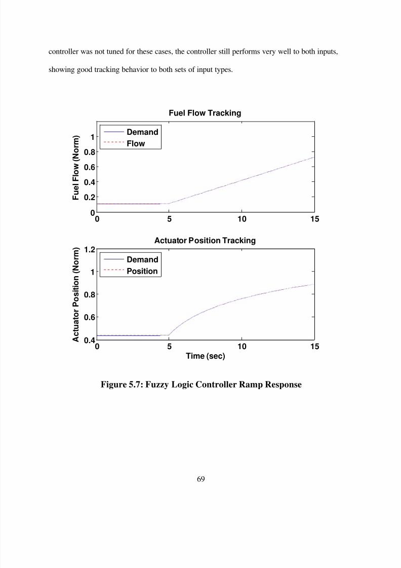
Citation preview

8/6/2019 Vick Andrew
http://slidepdf.com/reader/full/vick-andrew 1/99
UNIVERSITY OF CINCINNATI
Date:
I, ,
hereby submit this original work as part of the requirements for the degree of:
in
It is entitled:
Student Signature:
This work and its defense approved by:
Committee Chair:
11/19/2010 1,084
31-Aug-2010
Andrew W Vick
Master of Science
Aerospace Engineering
Genetic Fuzzy Controller for a Gas Turbine Fuel System
Kelly Cohen, PhDKell Cohen PhD
Andrew W Vick
8/6/2019 Vick Andrew
http://slidepdf.com/reader/full/vick-andrew 2/99

8/6/2019 Vick Andrew
http://slidepdf.com/reader/full/vick-andrew 3/99
i
Abstract
In this study, a fuel system controller for a gas turbine engine was examined. Controller design
in this application is challenging due to nonlinearities in the closed loop system, as well as
uncertainties associated with hardware components from part variation or degradation. Current
closed loop design methodologies are discussed, as are the limitations or challenges facing these
systems. Details on fuzzy logic control and its benefits in this type of application are explored.
Information on genetic algorithms is presented, along with a study on how this optimization
approach can be utilized to enhance the fuzzy logic controller process. A fuzzy logic controller
structure was developed for providing closed loop fuel control in the gas turbine application,
using a genetic algorithm to tune the system to provide an accurate and fast response to changing
input demands. With a genetic fuzzy controller in place, closed loop analysis was performed,
along with a stochastic robustness analysis to assess controller performance in an uncertain
environment. Results show that the genetic fuzzy system performed well in this application,
resulting in a system with fast rise and settling times to stepping inputs, while also minimizing
overshoot and steady state error. Robustness characteristics of the fuzzy controller were also
demonstrated, as the stochastic robustness analysis yielded acceptable performance in each
simulation of the closed loop system with uncertainties included.

8/6/2019 Vick Andrew
http://slidepdf.com/reader/full/vick-andrew 4/99
ii

8/6/2019 Vick Andrew
http://slidepdf.com/reader/full/vick-andrew 5/99
iii
Contents
List of Figures iv
1 Introduction 1
2 Background Information and Literature Survey 4
2.1 Current Design Methods 5
2.2 Fuzzy Logic Controller 12
2.3 Genetic Algorithm 27
2.4 Stochastic Robustness Analysis 38
3 Hardware Model Description and Formulation 42
4 Genetic Fuzzy System Approach 47
5 Controller Selection and Closed Loop Analysis 60
6 Controller Robustness Analysis 72
7 Conclusions and Future Research 82
References 87
8/6/2019 Vick Andrew
http://slidepdf.com/reader/full/vick-andrew 6/99
iv
List of Figures
2.1 Sample Membership Functions for Temperature 13
2.2 Membership Function Evaluation for Set Temperature 14
2.3 Fuzzy Logic Controller Structure 15
2.4 Output Fuzzy Sets for Water Heater Example 21
2.5 Non-Isosceles Fuzzy Membership Functions 24
2.6 Illustration of One-Point Crossover 31
2.7 Illustration of Two-Point Crossover 32
2.8 Illustration of Binary Mutation 32
2.9 Illustration of Genetic Inversion 33
2.10 Illustration of Population Selection and Genetic Variation Process 35
2.11 Illustration of Stochastic Robustness Analysis Process 41
3.1 Diagram of Closed Loop Fuel Control System 43
4.1 Symmetric Fuzzy Membership Functions 49
4.2 Non-Isosceles Fuzzy Membership Function Specification 50
4.3 Sample Non-Isosceles Fuzzy Membership Functions 54
5.1 Fitness Function Value History of Selected Fuzzy Controller 62
5.2 Performance Measure History of Selected Fuzzy Controller 62
5.3 Selected Fuzzy Membership Functions 64
5.4 Surface Plot of Selected Fuzzy Controller 66
5.5 Fuzzy Logic Controller Step Responses 67
5.6 Fuzzy Logic Controller Step Response Comparison 68

8/6/2019 Vick Andrew
http://slidepdf.com/reader/full/vick-andrew 7/99
v
5.7 Fuzzy Logic Controller Ramp Response 69
5.8 Fuzzy Logic Controller Sinusoid Response 70
6.1 Fitness Function Values for Each Monte Carlo Simulation 74
6.2 Histogram of Fitness Function Values 75
6.3 Step Input Results Comparison of Minimum, Maximum, and Base Cases 77
6.4 Histograms of Performance Parameter Values 78

8/6/2019 Vick Andrew
http://slidepdf.com/reader/full/vick-andrew 8/99
1
Chapter 1
Introduction
With the dawn and advancement of the industrial age, means for controlling mechanical systems
and processes have been sought. From early electronic circuits to modern digital controls,
systems have been developed to provide automation, improve accuracy, increase efficiency, or
expand capability. This trend is expected to continue, as new technological challenges are
undertaken.
Control systems cover a broad spectrum of applications, as well a broad spectrum of
involvement in a given system. Some control systems function merely in watchdog roles,
monitoring critical parameters in a system and taking mitigating action in the event an
unsatisfactory condition is detected. In other systems, the control system is absolutely critical to
the performance and capabilities of the system. In fact, many modern tactical aircraft are
designed to be aerodynamically unstable, and when augmented with a well-designed control
system, provide enhanced flying qualities and increased operational capabilities to give an edge
in their designed missions.
In an age driven by technology, where systems are constantly being pushed to meet new
challenging requirements, advancements in control system design are needed to keep up. We
want our mechanical systems to be faster, more accurate, and more robust. We want our systems
to be intelligent, to be able to analyze current conditions and objectives, and to make decisions

8/6/2019 Vick Andrew
http://slidepdf.com/reader/full/vick-andrew 9/99
2
on appropriate behavior, instead of just applying generic global behavior. To this end, intelligent
control techniques are gaining traction and increased focus.
Fuzzy logic control is one such intelligent control technique, and will be a pillar of this study.
This nonlinear control design technique provides significant benefits in terms of flexibility and
optimization space. When coupled with the ability to capture expert or heuristic knowledge, and
the ability to tune behavior in local envelopes of the operating space, fuzzy logic can be an
indispensable control design tool in many applications. Fuzzy logic control also possesses
inherent robustness properties due to having knowledge-based properties, making them good
candidates for stochastic systems.
As a result of the flexibility of fuzzy logic controllers, one challenge facing control designers is
the tuning process. Fuzzy logic controllers can have a variety of handles to impact performance,
from the fuzzy input and output sets to the governing rule base. Genetic algorithms, a branch of
evolutionary algorithms, will be utilized in this study to provide an autonomous guided search of
the design space to develop a more optimized solution against the design requirements. This
approach uses a search scheme based on evolutionary principles, a ‘survival of the fittest’ type
technique, including genetic recombination and variation.
In addition to ensuring a controller design meets performance requirements and objectives, a
designer will also want to make sure the controller will be robust enough to meet those
requirements in all operating conditions. A controller may perform admirably for a given
mechanical system design, but will it uphold that performance when part-to-part variation due to

8/6/2019 Vick Andrew
http://slidepdf.com/reader/full/vick-andrew 10/99
3
manufacturing capabilities is taken into account? Will it stand up to all operating conditions and
system degradation? A study in controller robustness is needed to answer these questions, and in
this study, a stochastic robustness analysis will be performed to ensure the controller maintains
adequate performance in an uncertain environment.

8/6/2019 Vick Andrew
http://slidepdf.com/reader/full/vick-andrew 11/99
4
Chapter 2
Background Information and Literature Survey
In this chapter, background information on current closed-loop control system design approaches
and methodologies will be presented, as well as some of the limitations on those systems.
Information on intelligent control techniques, Fuzzy Logic Control in particular, will also be
presented, including why these type systems are good candidates in the face of the limitations on
traditional design methods. Details on Genetic Algorithms and their use in fuzzy systems will
also be covered. Lastly, information will be presented on Stochastic Robustness Analysis, a
useful technique for characterizing controller performance robustness.

8/6/2019 Vick Andrew
http://slidepdf.com/reader/full/vick-andrew 12/99
5
2.1 Current Design Methods
Through its history, control system design has produced a wide variety of approaches and
techniques that can be used in various systems. In this section, a few of the more common and
broadly used schemes will be discussed. Basic background information on the approaches will
be covered, along with their benefits and constraints.
One of the simplest controller forms is an on-off controller, commonly referred to as a ‘bang-
bang’ controller. This type of controller has two states it can switch between, such as a heating
element switching on or off, or a valve switching between two positions. Implementation is
fairly straightforward, switching states whenever certain criteria are met. This type controller
has its roots in optimal control theory, and as such represents a minimal-time solution, making it
very effective in many design situations [21].
Even with its simple structure, this type controller has many applications. Many heating and air
conditioning systems run on a bang-bang controller, targeting a temperature band around a given
set point. For a residential heating system, the controller will turn on whenever the temperature
dips below the set point (perhaps with some hysteresis), adding heat to the system until the set
point is reached. The furnace then switches off, leaving the temperature of the system to float
until it drops below the trip point again. An air conditioning system works similarly, in the
opposite direction. Bang-bang controllers are more than adequate in these type scenarios, aided
by the relatively large time constants of the system under control (internal temperature).

8/6/2019 Vick Andrew
http://slidepdf.com/reader/full/vick-andrew 13/99

8/6/2019 Vick Andrew
http://slidepdf.com/reader/full/vick-andrew 14/99

8/6/2019 Vick Andrew
http://slidepdf.com/reader/full/vick-andrew 15/99
8
The final term, the derivative component, acts on the derivative of the current error. This piece
can be interpreted as a predictor of future error, and when combined with the past-capturing
properties of the integral term and the proportional term acting on the current error, provides a
controller with influence from all three time regions, a reason for the broad appeal of PID
controllers [2]. Incorporation of derivative control can help reduce overshoot and settling time to
stepping input demands, and can be used to balance the negative effects of the proportional and
integral terms in these areas. Derivative control can also improve stability properties of the
closed loop system.
It is not necessary to use all three components in every instance; the individual components can
be combined in any permutation to suit the needs of the control application at hand. Sometimes
only a simple proportional (P) controller is needed, or perhaps adding in an integral component
to help with steady state accuracy (PI controller). This freedom in design, along with their
simple structure and vast experience base, enable PID controllers to have a broad appeal.
Many controllers of this class can provide reasonable control in terms of stability with minimal
tuning, however many applications may have additional requirements in terms of timing,
overshoot, or error that may require additional tuning. Even though this type controller typically
has up to three parameters that influence behavior, tuning can become cumbersome to achieve
optimum operating points. Manual tuning is possible, but it is often best to start with a set of
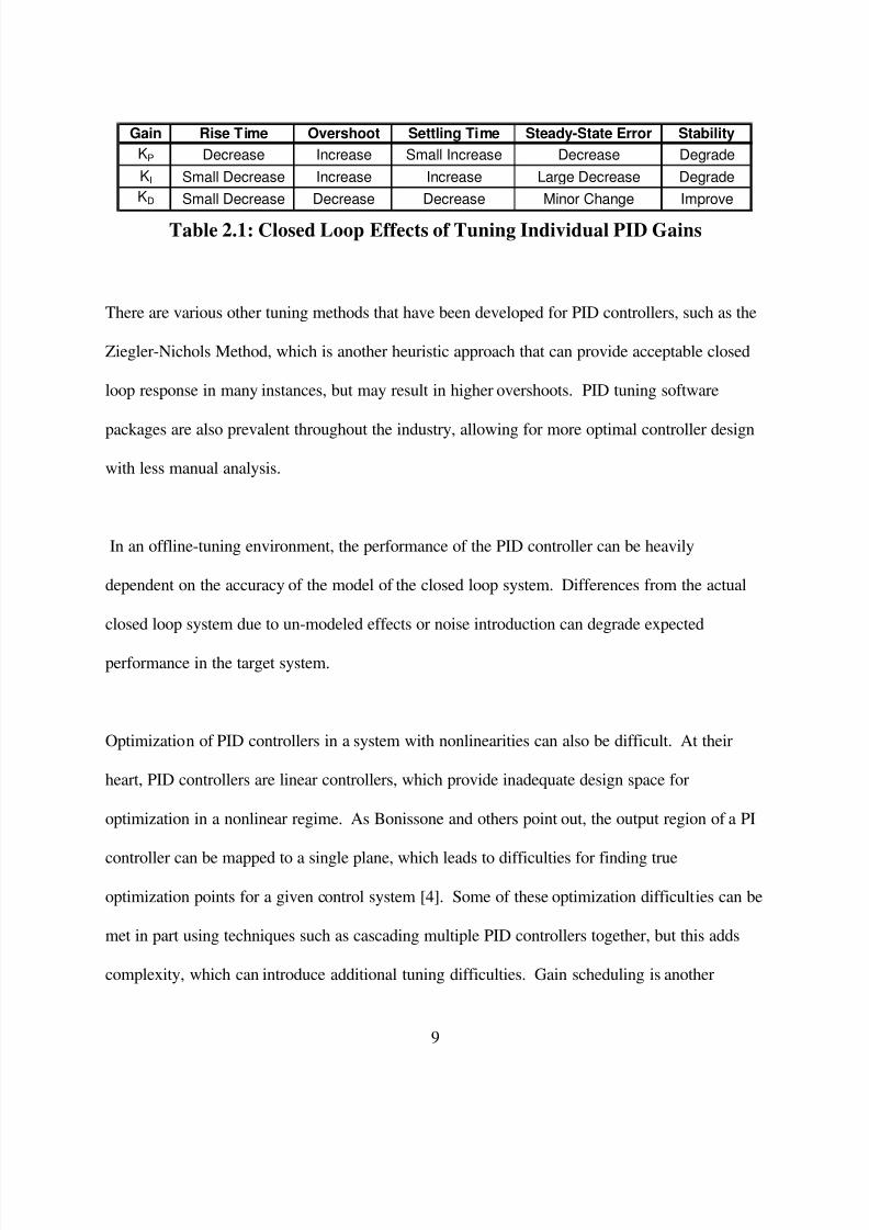
heuristics to serve as guidelines, such as shown in Table 2.1 suggested by Ang and others [1].
This table shows the impact of increasing an individual gain while holding the others constant.
8/6/2019 Vick Andrew
http://slidepdf.com/reader/full/vick-andrew 16/99
9
Table 2.1: Closed Loop Effects of Tuning Individual PID Gains
There are various other tuning methods that have been developed for PID controllers, such as the
Ziegler-Nichols Method, which is another heuristic approach that can provide acceptable closed
loop response in many instances, but may result in higher overshoots. PID tuning software
packages are also prevalent throughout the industry, allowing for more optimal controller design
with less manual analysis.
In an offline-tuning environment, the performance of the PID controller can be heavily
dependent on the accuracy of the model of the closed loop system. Differences from the actual
closed loop system due to un-modeled effects or noise introduction can degrade expected
performance in the target system.
Optimization of PID controllers in a system with nonlinearities can also be difficult. At their
heart, PID controllers are linear controllers, which provide inadequate design space for
optimization in a nonlinear regime. As Bonissone and others point out, the output region of a PI
controller can be mapped to a single plane, which leads to difficulties for finding true
optimization points for a given control system [4]. Some of these optimization difficulties can be
met in part using techniques such as cascading multiple PID controllers together, but this adds
complexity, which can introduce additional tuning difficulties. Gain scheduling is another
Gain Rise Time Overshoot Settling Time Steady-State Error Stability
KP Decrease Increase Small Increase Decrease Degrade
KI Small Decrease Increase Increase Large Decrease Degrade
KD Small Decrease Decrease Decrease Minor Change Improve

8/6/2019 Vick Andrew
http://slidepdf.com/reader/full/vick-andrew 17/99
10
option, which modifies the PID gains depending on certain conditions, which incorporates
techniques similar to intelligent control, discussed later in this study.
Robustness is a concern in any controller design application, and this is no different for PID
controllers. This type of controller can have a difficult time dealing with uncertainty in the
closed loop system. Small shifts in characteristic parameters of the closed loop system can shift
the controller to a lower performance point, or could erode stability margins. Intelligent control
techniques, such as fuzzy logic controllers, have some inherent improvements in robustness
characteristics, and may be a better fit in stochastic systems. Work has been done in the area of
fuzzy-PID controllers, providing the benefits of the PID structure with the added robustness and
flexibility that results from the nonlinear fuzzy structure [28].
There are a number of other closed-loop control schemes besides bang-bang and PID controllers,
although the design of these systems is often more involved than these simple forms, and they
are not as widely used. One such approach is Optimal Control, which, as the name would
suggest, is a technique that tries to operate at the most optimized conditions, such as a minimum
time or minimum fuel burn case. Paiewonsky provides some background into optimal control
theory, as well as a variety of examples illustrating application [14].
Robust control is another control design approach, one that tries to ensure controller stability in
the face of uncertainty in the closed loop system. This approach assumes a bounded distribution
for system disturbances, and is designed to maintain adequate control over any disturbance
within the range. H-infinity loop-shaping is the most common robust control technique, and is

8/6/2019 Vick Andrew
http://slidepdf.com/reader/full/vick-andrew 18/99

8/6/2019 Vick Andrew
http://slidepdf.com/reader/full/vick-andrew 19/99
8/6/2019 Vick Andrew
http://slidepdf.com/reader/full/vick-andrew 20/99
13
0 20 40 60 80 100
-0.2
0
0.2
0.4
0.6
0.8
1
1.2
1.4
Temperature Membership Functions
Temperature (°C)
M e m b e r s h i p
Cold
Warm
Hot
Figure 2.1: Sample Membership Functions for Temperature
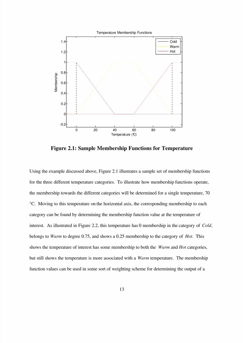
Using the example discussed above, Figure 2.1 illustrates a sample set of membership functions
for the three different temperature categories. To illustrate how membership functions operate,
the membership towards the different categories will be determined for a single temperature, 70
°C. Moving to this temperature on the horizontal axis, the corresponding membership to each
category can be found by determining the membership function value at the temperature of
interest. As illustrated in Figure 2.2, this temperature has 0 membership in the category of Cold ,
belongs to Warm to degree 0.75, and shows a 0.25 membership to the category of Hot . This
shows the temperature of interest has some membership to both the Warm and Hot categories,
but still shows the temperature is more associated with a Warm temperature. The membership
function values can be used in some sort of weighting scheme for determining the output of a

8/6/2019 Vick Andrew
http://slidepdf.com/reader/full/vick-andrew 21/99
14
system based on this input temperature, or also can be used in a Fuzzy Logic Control system,
which will be demonstrated shortly.
0 20 40 60 80 100
-0.2
0
0.2
0.4
0.6
0.8
1
1.2
1.4
Temperature Membership Functions
Temperature (°C)
M e m b e r s h i p
Cold
Warm
Hot
Figure 2.2: Membership Function Evaluation for Set Temperature
Membership function categories and their values are up to the designer, and could be adjusted
based on system needs. In the example above, trapezoidal membership functions were used
(truncated for limits), but membership functions can take a number of different forms. Isosceles
triangles are fairly common, but it is possible to use non-isosceles triangles as well. Gaussian
distributions and exponential distributions are also available for use to the designer following
scaling, as well as any custom function with values over the interval from [0 1].
Mamdani expanded on Zadeh’s use of fuzzy sets to develop a control system based on fuzzy
logic principles [10]. A Fuzzy Logic Control system can operate in a closed loop environment
8/6/2019 Vick Andrew
http://slidepdf.com/reader/full/vick-andrew 22/99

8/6/2019 Vick Andrew
http://slidepdf.com/reader/full/vick-andrew 23/99
16
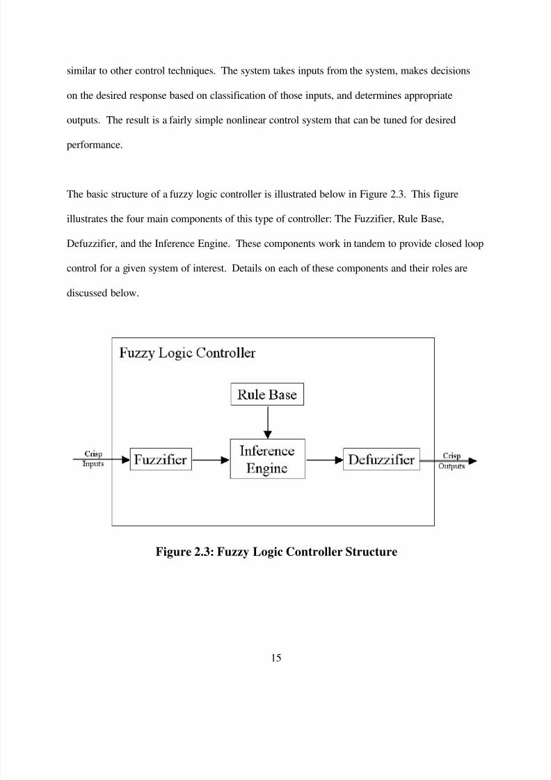
Fuzzifier:
The purpose of the fuzzifier is to transform the crisp inputs into the fuzzy logic controller into
fuzzy inputs. The inputs to this type of system can range from sensed quantities, estimated
quantities, or even system demands for a desired state. The fuzzifier uses series of membership
functions to categorize the crisp inputs into their respective fuzzy set representations. The
fuzzifier determines which fuzzy sets are ‘active’ (non-zero membership) based on each of the
crisp inputs, and also to what degree. The membership function example using the temperature
scale could be viewed as a sample fuzzifier. The crisp input coming in would be the
temperature, measured using a sensor or estimated from a mathematical model. As shown, the
output would be the membership function values associated with each fuzzy set.
Fuzzifiers must provide coverage of the input space; every potential input to the fuzzy system
must result in membership to one or more of the possible fuzzy sets. This helps ensure
completeness for the fuzzy logic control system, to be discussed in more detail in the section on
rule bases. Computation is also an important consideration when designing a fuzzifier. For each
fuzzy set that becomes active based on a given input, the mathematics of the inference engine
become more involved as a result, especially when considering controllers with multiple inputs,
with different fuzzy sets associated with each. Therefore, it is standard practice to ensure that
only two fuzzy sets are active at a time for each input, leading to the guideline that only adjacent
fuzzy sets should be allowed to overlap in their membership function distributions.

8/6/2019 Vick Andrew
http://slidepdf.com/reader/full/vick-andrew 24/99

8/6/2019 Vick Andrew
http://slidepdf.com/reader/full/vick-andrew 25/99
18
This rule base is fairly crude, and may not deliver adequate performance in all driving
conditions. Enhancements to this rule base may involve adding more fuzzy sets to the input and
output systems, increasing granularity. For example, modified categories like Very Low or
Slightly High could be added as additional fuzzy sets to the fuzzifier, and the output could be
expanded to include additional classes for Accelerate and Decelerate, perhaps to provide varying
degrees of these actions. Another option would be to include an additional input to the fuzzifier,
perhaps a rate term in addition to the speed difference. Examples of rules using these expanded
fuzzy sets could include statements such as “IF speed delta is Slightly Low AND speed is
Increasing, THEN Maintain” or “IF speed delta is Slightly Low AND speed is Decreasing,
THEN Accelerate”. This could provide a means of differentiating different driving cases,
leading to different controller behavior dependent on a given scenario. While this example is
fairly basic and not complete, it should provide insight into the rule-making process and how
working knowledge of a system could be captured without the need for expertise in control
system design.

8/6/2019 Vick Andrew
http://slidepdf.com/reader/full/vick-andrew 26/99
19
Defuzzifier:
The defuzzifier fulfills the inverse role of the fuzzifier; it takes the information from the fuzzy
output sets and transforms them into crisp outputs that can be used by the control system. This
output could be a number of different things, from controller loop gains, to modeled parameters,
to the system demands themselves. The typical defuzzifier consists of membership functions
similar to a fuzzifier, but the system works in the opposite direction. Instead of working from
the input on the horizontal axis to determine the fuzzy set memberships, the active fuzzy sets are
used to find a crisp output on the horizontal axis. The active fuzzy sets in the defuzzifier are
determined by the rule consequents in the inference engine, and some mathematical approach is
used to combine these sets into a single output value. A Centroid method is one of the more
common and simplistic approaches, and will be employed in this study and demonstrated below.
Numerous other methods have been proposed as alternatives to try to accommodate some of the
potential pitfalls or special cases that can arise [11].

8/6/2019 Vick Andrew
http://slidepdf.com/reader/full/vick-andrew 27/99
8/6/2019 Vick Andrew
http://slidepdf.com/reader/full/vick-andrew 28/99
21
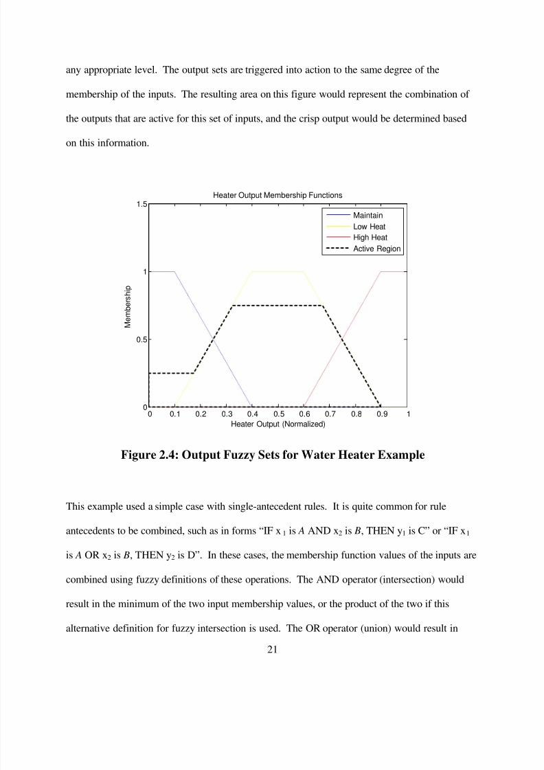
any appropriate level. The output sets are triggered into action to the same degree of the
membership of the inputs. The resulting area on this figure would represent the combination of
the outputs that are active for this set of inputs, and the crisp output would be determined based
on this information.
0 0.1 0.2 0.3 0.4 0.5 0.6 0.7 0.8 0.9 10
0.5
1
1.5Heater Output Membership Functions
Heater Output (Normalized)
M e m b e r s h i p
Maintain
Low Heat
High Heat
Active Region
Figure 2.4: Output Fuzzy Sets for Water Heater Example
This example used a simple case with single-antecedent rules. It is quite common for rule
antecedents to be combined, such as in forms “IF x1 is A AND x2 is B, THEN y1 is C” or “IF x1
is A OR x2 is B, THEN y2 is D”. In these cases, the membership function values of the inputs are
combined using fuzzy definitions of these operations. The AND operator (intersection) would
result in the minimum of the two input membership values, or the product of the two if this
alternative definition for fuzzy intersection is used. The OR operator (union) would result in

8/6/2019 Vick Andrew
http://slidepdf.com/reader/full/vick-andrew 29/99
22
maximum of the two input membership values being used, or any one of a number of alternative
definitions [11]. Of course, these operators could be expanded to whatever number of rule
antecedents are used for a given rule base system.
As with any new design approach, it will have benefits and drawbacks compared to other design
methods. Fuzzy logic controllers allow for a simple implementation of a nonlinear control
system design. This approach is also a candidate for embedded systems because of its relative
ease for computation. The structure of this type of controller also provides for
compartmentalization, leading to the possibility of the controller to be tuned for specific behavior
in smaller, local operating regions, instead of having to tune or check the performance over the
entire operating envelope following controller adjustments [27]. Fuzzy logic controllers are also
able to perform admirably in the face of uncertainty in a given control application, making them
good candidates for systems that need to meet higher performance objectives in environments
affected by uncertainties.
Fuzzy logic controllers have been explored and implemented for a number of different
applications. Kelly, Weller, and Ben Asher develop a controller for a linear second-order system
proposed as a benchmark problem by the American Control Conference [6]. This problem
consisted of a system with plant uncertainty, and had a non-colocated sensor and actuator pair,
leading to a nontrivial design problem. They cite a fuzzy logic controller as a good candidate for
this application due to its ease of implementation, and its inherent robustness characteristics.
Also mentioned is the ability of the controller to emulate the minimum-time solution derived
from optimal control theory using heuristics in its rule base. The controller in this paper was

8/6/2019 Vick Andrew
http://slidepdf.com/reader/full/vick-andrew 30/99
23
developed with a Luenberger observer in the loop; the current study will have access to
necessary control states. Following controller development, the paper also examined the
robustness characteristics of the control system through Stochastic Robustness Analysis,
examined further in this study.
Nelson and Lakany have studied use of fuzzy logic in the fuel control system for industrial gas
turbines [12]. In their paper, they discuss how traditional control system design methods may
encounter difficulties in systems that can degrade over time, especially in areas of emissions
control. They suggest that fuzzy logic controllers may be a good candidate for this type of
environment, lending to their nonlinear properties and robustness in cases where the plant may
not be well understood (as in cases of degradation). They develop a fuzzy logic controller to
compare performance against an existing PI controller. Through various operational scenarios,
performance of the two controllers was comparable, although the PI controller typically had
better response and settling times. In some scenarios, however, the fuzzy logic controller did
show better performance in terms of exhaust temperature overshoot, which is a critical
performance measure in industrial gas turbine operation.
A key comment Nelson and Lakany mention in their paper is the difficulty to tune the fuzzy
logic controller to a more optimum design point. They implemented a controller with two
inputs, Error and Error Rate ( E and ö ), using five fuzzy sets for each. The output, an incremental
change to fuel demand, also had five sets, although singleton sets were used. The system used
25 rules in the base for the inference engine. The result is a large number of parameters that can
be tuned to affect performance, although some simplifications were made.
8/6/2019 Vick Andrew
http://slidepdf.com/reader/full/vick-andrew 31/99
24
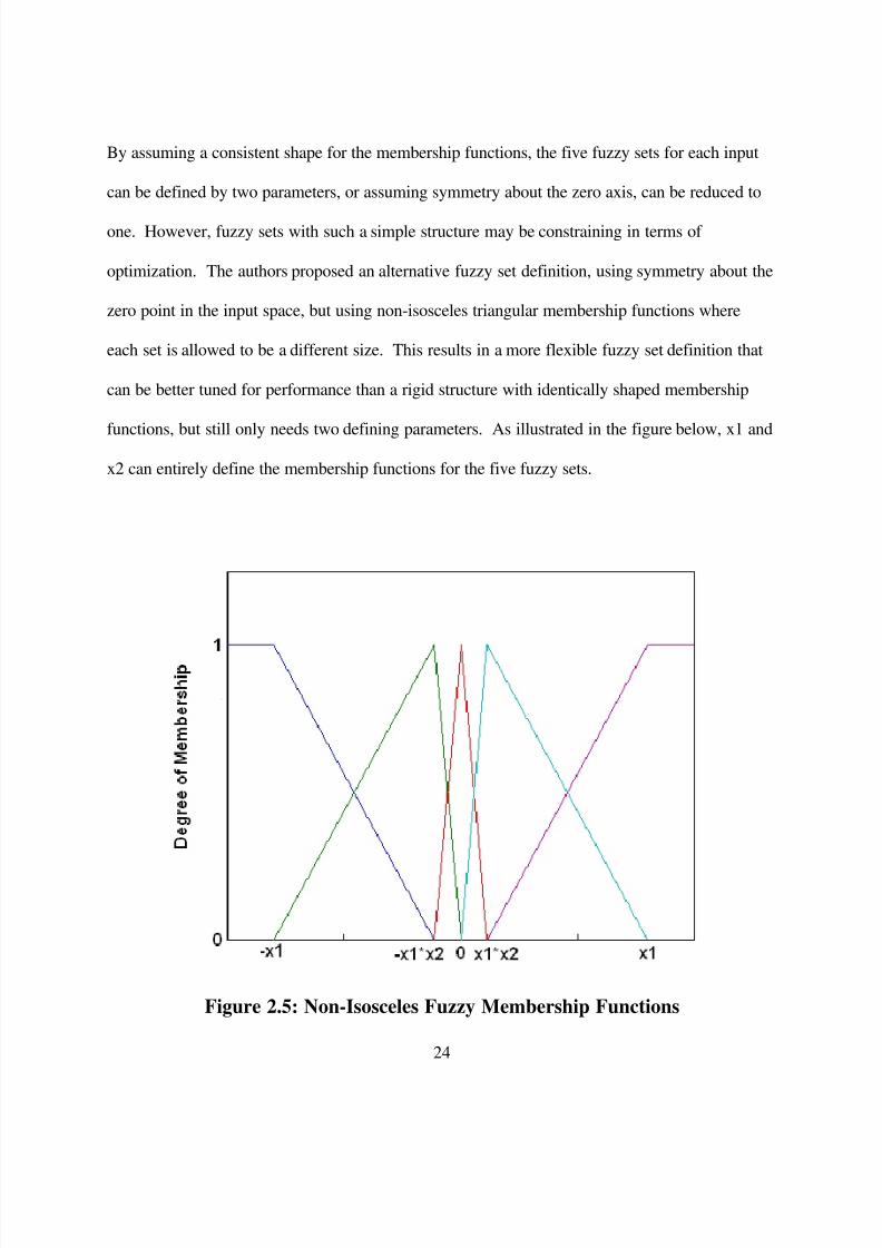
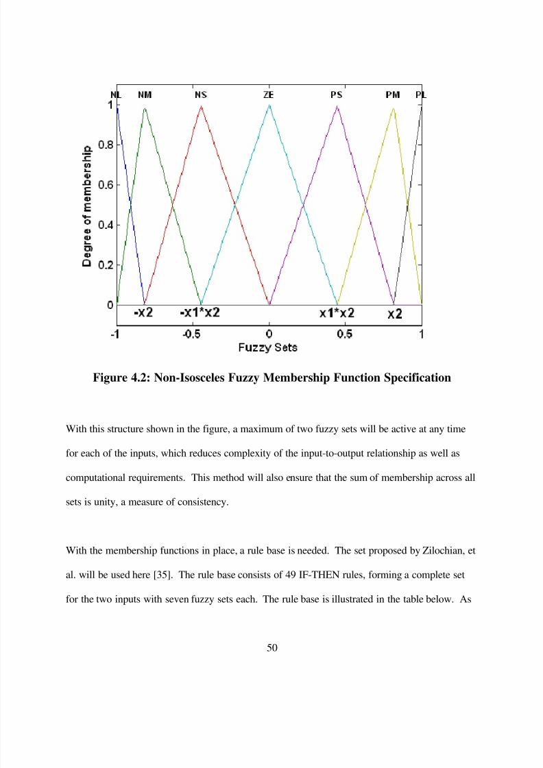
By assuming a consistent shape for the membership functions, the five fuzzy sets for each input
can be defined by two parameters, or assuming symmetry about the zero axis, can be reduced to
one. However, fuzzy sets with such a simple structure may be constraining in terms of
optimization. The authors proposed an alternative fuzzy set definition, using symmetry about the
zero point in the input space, but using non-isosceles triangular membership functions where
each set is allowed to be a different size. This results in a more flexible fuzzy set definition that
can be better tuned for performance than a rigid structure with identically shaped membership
functions, but still only needs two defining parameters. As illustrated in the figure below, x1 and
x2 can entirely define the membership functions for the five fuzzy sets.
Figure 2.5: Non-Isosceles Fuzzy Membership Functions

8/6/2019 Vick Andrew
http://slidepdf.com/reader/full/vick-andrew 32/99
25
Of course, this approach can be expanded for inputs with more fuzzy sets, adding an additional
tuning parameter for each pair of additional sets. The symmetry constraint is common in fuzzy
logic controller designs, as it is often desired to have consistent system response when moving in
different directions. This approach may still provide some constraints on a truly optimal
solution, but it does add flexibility to the design space and ensures that total membership across
fuzzy sets always sums to one, which can be an important factor for controller consistency.
A fuzzy logic controller for a fuel system test bench is developed in an article by Zilouchian and
others [35]. This test bench is designed to allow for proper simulation testing of a jet engine fuel
delivery system, by controlling the combustor pressure that would be experienced in a given
operating condition. The fuel system test bench is currently controlled with a traditional PI
controller, but performance shortfalls are noted. This paper looks to fuzzy logic as a solution due
to its nonlinear characteristics and the ability for tuning in small operating envelopes
(compartmentalization). The authors also make note of the difficulties in tuning fuzzy logic
controllers due to the number of design options. In this paper, they chose to use a consistent
structure of seven triangular membership functions with equal size normalized over the range [-
1, 1] for both the inputs (Error and Change in Error, E and ∆E) and output (Valve Positions), and
chose to optimize using a scaling parameter up and downstream of the fuzzy sets. This restricts
flexibility, but provides a simple structure for a first cut at controller design. The authors went
on to develop separate fuzzy logic controllers for ‘coarse’ and ‘fine’ control, utilizing the
compartmentalization capabilities of fuzzy logic schemes.

8/6/2019 Vick Andrew
http://slidepdf.com/reader/full/vick-andrew 33/99
26
As discussed above, one of the major drawbacks to a fuzzy logic controller cited in various
sources is the tuning process. The membership function types and the distributions themselves
can present a great number of design options for the input/output fuzzy systems, which can be
paralyzing for a designer trying to optimize a given control system. The rule base provides
another set of inputs that can be used to alter the performance of the loops. Use of genetic
algorithms can help in this area, performing a guided search towards an optimal design and
taking some of the burden off of the control system designer. Details of genetic algorithms will
be discussed in the next section.

8/6/2019 Vick Andrew
http://slidepdf.com/reader/full/vick-andrew 34/99
27
2.3 Genetic Algorithm
Genetic Algorithms are a class of optimization approaches based on evolutionary principles.
First introduced by John Holland in 1975, this type of algorithm searches for an optimized
solution based on the premise of “survival of the fittest” [8]. The approach emulates Charles
Darwin’s research on natural selection, that those members of a population best suited for their
environment are more likely to survive and pass on their genetic traits. In a genetic algorithm,
members of a population are represented by numeric strings (dubbed chromosomes), and
evaluated for fitness for a certain function. Similar to natural selection, those that receive higher
fitness ratings are more likely to see their chromosomes passed on to subsequent generations of
the population, and through an iterative process, this algorithm will converge to a better
performing design. This algorithm also incorporates the ideas of genetic variation, which will be
discussed further in this chapter.
One of the first steps in developing a genetic algorithm is to determine how members of the
population will be represented. Binary strings are the most common and often simplest
representation, but it is also possible to represent members of the population with non-binary, or
real-value coded strings. Fixed-length strings are more common, but Cordon, and others discuss
details of variable-length strings and their benefits and application [7]. For this study, fixed-
length binary-coded strings will be employed in the optimization algorithm for their inherent
simplicity.

8/6/2019 Vick Andrew
http://slidepdf.com/reader/full/vick-andrew 35/99
28
One problem that can arise when using a binary-coded string in the traditional base-two sense is
related to the large hamming distances that are realized for successive integers. Integer values 7
and 8 for example have binary representations of 0111 and 1000 respectively, illustrating a
difference in every character in the string for a relatively small difference in numeric value. The
iterative genetic algorithm process may have a difficult time converging to a true optimized point
using basic genetic variations (discussed below) if it would have to cross a large hamming
distance en route. Cordon and others propose the use of a gray code, in which only hamming
distances of 1 separate successive integers [7]; however, single bit value changes may still have a
large impact on the represented numeric value. This study will utilize multiple runs of the
genetic algorithm, each with a different random initial population to try to mitigate this
shortcoming.
Once the representation format for the members of the population has been determined, the
initial population needs to be generated. The number of members in the population is left up to
the designer. Larger populations will provide more opportunities to search the design space and
provide population variation, but will also take longer to determine performance and the makeup
of successive populations. The initial set can be generated in a number of different ways,
ranging from purely random generation for each member string, to sparse sets that try to cover
the range of the design space, or even initial predetermined candidate sets that correspond to
known performance levels for which improvement is desired. Hybridization of these methods
can also be utilized to generate an initial population.
8/6/2019 Vick Andrew
http://slidepdf.com/reader/full/vick-andrew 36/99
29
With the initial population in place, the next step is to develop a means of assessing the
performance of each member for a given function. A common example could be a genetic
algorithm that tries to minimize the time for a given process. For this type case, the fitness
function could simply be the inverse of the calculated time, yielding higher fitness ratings
corresponding to members with the lowest process times. In this study into closed loop control
applications, the fitness function will be based on common controller performance metrics such
as response time, settling time, and control efforts.
As future populations are often developed using probabilities of selection based on the fitness
ratings, it may be important to ensure that the fitness values are all positive. Another common
pitfall in the optimization process is for a member to stand out from other members in terms of
vastly superior fitness rating, which can lead to premature convergence if it occurs in early
generations depending on the selection schemes used. Also, in later generations when most
members begin to illustrate improved performance, it may make it difficult for any particular
member to stand out, slowing the process of convergence to an optimized solution. As a means
for mitigating these scenarios, Cordon and others provide suggestions for a number of fitness
function scaling methods [7].
With the performance for a current population known, this information can be used to determine
the candidate makeup of the next generation. Some selection schemes place direct copies of the
top performers of a population into the subsequent population, known as elitist selection,
ensuring that best performer of the next generation is always at least as good as the one before it.
This approach also ensures that the candidate pool contains the genetic strings of the best known

8/6/2019 Vick Andrew
http://slidepdf.com/reader/full/vick-andrew 37/99
30
solutions are always available for future generations, immune to being removed due purely to
random occurrence. Similarly, discarding the poorest performers is another option, although
these candidates may still have some desirable qualities that could become part of future
solutions, and would tend to be removed from future generations anyway as part of the genetic
algorithm process.
Most selection schemes choose candidates from the existing population using a probability
measure determined from their fitness. The simplest of these measures is to divide the fitness of
a given candidate by the sum of fitness for all candidates, although other probability
methodologies have been suggested [7]. Using the simple approach, the candidates can then be
thought of as being arranged on a roulette wheel, filling area proportional to their probability
level. The wheel is then spun to select a candidate as many times as needed to fill out the full
population.
This roulette wheel approach has some inherent flaws, one being the potential for large
discrepancy between the expected and actual number of selections for a given candidate.
Alternative methods for selection have been proposed, one of which being stochastic universal
sampling [7]. In this sampling method, the roulette wheel is only spun once, while pointers
spaced equi-circumferentially around the wheel determine the candidates needed to fill the
population. There are numerous other schemes that can be employed in the selection process,
each trading off simplicity for the likelihood of a better population sample.

8/6/2019 Vick Andrew
http://slidepdf.com/reader/full/vick-andrew 38/99
31
With the candidates for the next generation of a population selected from the previous, the
genetic variation process begins. Three different processes will be used to introduce genetic
variation into the existing candidates: crossovers, mutations, and inversions.
Crossovers involve swapping genetic material between two chromosomes. In this way, optimal
solutions are sought in the area of current knowledge in the design space. The simplest of these
is the one-point crossover, where a number less than the length of the chromosome strings is
chosen at random, and the genetic strings to the right of that number are swapped between two
parent chromosomes. This is illustrated in Figure 2.6 below for two sample binary strings
swapping the rightmost two bits.
Figure 2.6: Illustration of One-Point Crossover
The two-point crossover is also common, and helps alleviate the bias that the latter part of the
chromosome strings are more likely to be swapped. In this process, two random numbers are
chosen, and the string of characters between the two numbers is swapped in the parent
chromosomes, as illustrated in Figure 2.6. Of course, this process could be extrapolated for
higher order crossovers, up to the limiting case of the uniform crossover , where the child
Chromosome A Chromosome A'
1 0 1 1 0 0 1 0 1 1 1 1
Chromosome B Chromosome B'
1 1 1 0 1 1 1 1 1 0 0 0

8/6/2019 Vick Andrew
http://slidepdf.com/reader/full/vick-andrew 39/99

8/6/2019 Vick Andrew
http://slidepdf.com/reader/full/vick-andrew 40/99

8/6/2019 Vick Andrew
http://slidepdf.com/reader/full/vick-andrew 41/99
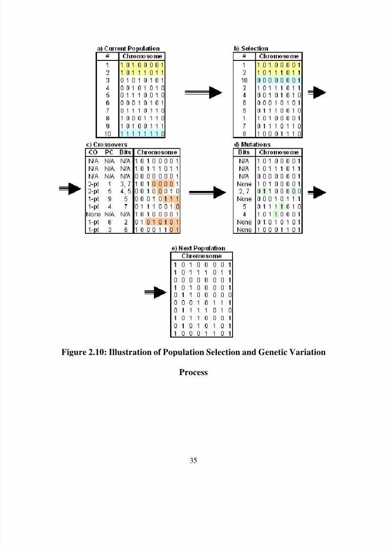
34
population are selected with some randomness from the current members, typically weighted in
some fashion using the current populations’ fitness ratings. Part b) shows the resulting
chromosomes from the selection process.
Following selection, the population (minus elites and inverts) is subjected to crossovers. A
random number is generated for each chromosome, and compared to the probability number
selected for crossovers. For this example, both one- and two-point crossovers were employed.
Part c) of Figure 2.10 shows the results of the crossover phase. The first column (CO) indicates
which type of crossover resulted (one-point, two-point, or none), the second column (PC)
indicated the partner chromosome with which genetic material was swapped, and the third (Bits)
shows which bits bound the crossover.
Part d) of the figure illustrates the mutation phase. A random number is generated for each bit of
each member of the population, and compared to the selected probability for mutations. Each bit
that meets the criteria is inverted, as illustrated in the first column of the figure. This phase
completes the process for generating the next population, which is illustrated in Part e) of Figure
2.10.
8/6/2019 Vick Andrew
http://slidepdf.com/reader/full/vick-andrew 42/99

8/6/2019 Vick Andrew
http://slidepdf.com/reader/full/vick-andrew 43/99
36
Genetic algorithms or other types of evolutionary-based techniques have been used as an
optimization tool in a number of different applications. Cordon and others illustrate a simple
example for path optimization under gravitational influence [7]. The genetic algorithm tries to
define the path for minimum time travel between two points. The path is discretized using a
number of intermediate points, with each point represented by a six-character binary string using
a simple base 2 encoding. Using an initial population of 20 individuals developed randomly,
successive populations are determined using an elitist scheme and using only one-point
crossovers and mutations as genetic operators. The time to travel between each point is
determined and the total summed, using the inverse of this path time as the fitness function. The
results were determined from a number of different initial populations, but the minimum paths
found were always relatively close to each other, illustrating the robustness of the process.
Nyongesa examines optimization of fuzzy-neural systems using genetic algorithms and other
evolutionary strategies [13]. The author describes the benefits of fuzzy logic controllers in areas
such as nonlinear behavior and the ability to capture expert or system knowledge. By
incorporating neural network capabilities, which are renowned for their knowledge acquisition
and adaptive learning capabilities, the paper discusses how fuzzy systems can be further
enhanced for robustness and performance in uncertain environments, but points out that
optimization of such a system is still cumbersome. Citing genetic and evolutionary algorithms,
the author discusses how these techniques can be incorporated to develop fuzzy-neural systems
optimized for a given application.

8/6/2019 Vick Andrew
http://slidepdf.com/reader/full/vick-andrew 44/99
37
Genetic algorithms have been used to help mitigate the effort associated with fuzzy logic system
optimization, collectively known as genetic fuzzy systems. In their paper on diesel engine
pressure modeling, Radziszewski and Kekez describe the use of genetic fuzzy systems to
develop an accurate model of the complex pressure profiles experienced in the diesel engine
cycle [16]. Fuzzy logic was fitting for the application due to its ability to represent nonlinear
systems, and also for robustness properties as several different fuel sources were used in the
engine modeling. Use of genetic algorithms allows for an easier method for tuning the various
fuzzy system parameters (membership functions and rule base) to generate an accurate model of
the pressure cycle that was robust enough across several different fuel types. As a fitness
function, the authors used a measure of accuracy to experimental data, along with a factor
associated with the number of rules in the resulting rule base, such that systems with fewer rules
may be rewarded for simplicity. The results consisted of several different genetic fuzzy system
models that met desired accuracies over specified ranges.

8/6/2019 Vick Andrew
http://slidepdf.com/reader/full/vick-andrew 45/99

8/6/2019 Vick Andrew
http://slidepdf.com/reader/full/vick-andrew 46/99

8/6/2019 Vick Andrew
http://slidepdf.com/reader/full/vick-andrew 47/99
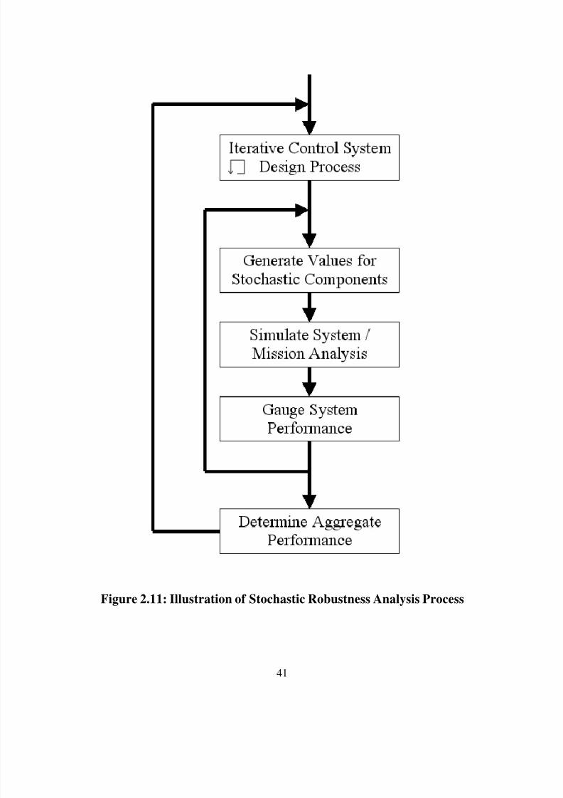
40
system information would make up one sample of the system, such as a member of a fleet or a
certain operating condition. With the system characteristics fully defined, simulation or mission
analysis can be performed as a means of determining performance. Following simulation,
stability or other performance measures can be assessed.
These steps make up one iteration of the analysis, typically refered to as a Monte Carlo analysis.
This process is then repeated as many times as the designer would like, with the benefit of
increased confidence coming with increased simulations. Once the system and uncertainty
distributions are set up, the only cost to additional iterations is computational time, which is
becoming less of an issue with increases in processing capabilities.
Once all of the Monte Carlo runs have been completed, the performance of the controller with
respect to the various selected measures for each run can be combined to develop an overall
sense of robustness across the simulated conditions. If performance against each measure was
assessed in a binary sense (pass/fail), then the binomial distribution can be used to aggregate
controller performance across all the runs. Based on these results, the control designer can then
determine whether performance was adequate across the sampling, or if additional adjustments
are needed. This process can also highlight regions of the design space that may be more critical
in terms of meeting requirements, where additional information about the limiting conditions
may lead to a better overall design.
8/6/2019 Vick Andrew
http://slidepdf.com/reader/full/vick-andrew 48/99
41
Figure 2.11: Illustration of Stochastic Robustness Analysis Process

8/6/2019 Vick Andrew
http://slidepdf.com/reader/full/vick-andrew 49/99
42
Chapter 3
Hardware Model Description and Formulation
In this study, a closed loop controller will be developed for a gas turbine fuel system. Turbine
engines often have multiple variable geometries, each with their own set of controlling hardware,
but rarely do these systems compare to the design challenges of the fuel system. Fuel control is
directly tied to gas turbine performance and operability, and is often associated with engine
constraints as well.
The hardware models for the gas turbine fuel system that will be used in this study are physics-
based. The models are initially developed from first principles, and later fine tuned once testing
data becomes available. Details of each of the components of the closed loop system are
modeled, including nonlinear characteristics. As with any manufactured system, some degree of
uncertainty is expected due to part-to-part variation and operating condition variation. These
uncertainties are included in the model for controller performance and robustness analysis.
The actuation system consists of an electro-hydraulic servo valve (EHSV), a single actuator, and
a throttling valve (also known as a Fuel Metering Unit, FMU). The EHSV takes an electrical
current signal from the controller and provides corresponding fuel flow to the actuator. The
actuator slides based on the flows and adjusts the fuel port areas as a function of stroke. The
throttling valve works to maintain a constant fuel pressure across the actuator fuel ports, which
yields a predictable fuel flow for a given port area. This fuel flow leads to a series of manifolds

8/6/2019 Vick Andrew
http://slidepdf.com/reader/full/vick-andrew 50/99
43
and eventually to the combustor’s fuel nozzles. The actuator position is fed back to the
controller through a linear variable displacement transducer, or LVDT. The diagram below
shows a simple schematic of the closed loop system.
Figure 3.1: Diagram of Closed Loop Fuel Control System
In the EHSV model, a null current is subtracted from the input current from the controller, and
then passes through a hysteresis model to account for current direction changes. This current
then passes through the first of two first-order lags to account for current rise time. The lagged
current value is input into an interpolating lookup table to determine the corresponding fuel flow,
and to which side of the actuator it is flowing. This lookup is linear over large regions, but does
have some nonlinear effects near the zero crossing as well as the end points. The calculated flow
is corrected for pressure and density conditions as compared to the rated conditions. The
resulting flow passes through a second first-order lag, the output of which is the flow to the
actuator.
There are a number of uncertainties associated with the EHSV model. Part-to-part variation can
lead to slight differences in null current level as well as the magnitude of the hysteresis term,
leading to instances of uncertainty. The time constants on the two first-order lags are also

8/6/2019 Vick Andrew
http://slidepdf.com/reader/full/vick-andrew 51/99
44
modeled with uncertainty to account for fleet variation. A gain modifier on the flow output of
the EHSV is also included, centered on unity.
The actuator model is fairly simple and straightforward; the flow provided by the EHSV is
divided by the actuator bore area, and integrated to determine the actuator stroke position. The
actuator stroke can be correlated to a fuel port area, and the resulting flow is related to the
pressure across this area. Uncertainty in the actuator is tied to bore and cylinder area variations
combined with frictional differences, but the levels of these are very small in comparison to
some of the other uncertainties in the loop, so they will not be considered in this study.
The throttling valve introduces additional nonlinearities and uncertainties, but these
characteristics are all downstream of the closed loop system. The actuator position is the
feedback used by the control, the fuel flow output of the system is not measured. The high level
closed loop control can adjust fuel flow demands by using other sensed quantities in the gas
turbine, so the dynamics of the throttling valve will not be considered for this study on the inner
loop controller.
The sensing system model consists of a second-order lag to represent the LVDT. Uncertainty is
included in this model as well, variation taken into account in both the natural frequency and
damping terms. The output of the LVDT is a pair of voltage signals corresponding to the
position of the actuator. It is customary to model noise on these signals, but this factor was left
out of the model for this study.

8/6/2019 Vick Andrew
http://slidepdf.com/reader/full/vick-andrew 52/99
45
Usually in this type of system, the controller hardware itself can introduce some slight dynamics
to the closed loop system. However, in many cases such as this instance, the contribution is
small compared to the other components in the system. As a result, the dynamics from the
control hardware will be neglected in this study.
Also in this study, normalization will be applied to the actuator position and the fuel demands
and resulting flows. This gives the results a more universal appeal without getting caught up in
details of the specific application.
The current controller for this fuel system is a Proportional-Integral (PI) controller. As discussed
in Chapter 2.1, the proportional component is implemented to try to give fast response times to
changing demands, and the integral component is in place to try to eliminate steady state error.
Derivative control elements can be difficult to design for this type of system. As mentioned
above, the voltage feedback signals are susceptible to noise, which present a challenge for
mathematical derivatives. It is possible to filter out some of the noise, but its not a trivial task,
and can reduce the effectiveness of the derivative component. For the current system, control
can be achieved without this component.
The current controller doesn’t use fixed gains for proportional and integral components. Instead,
the controller employs a technique known as gain scheduling. With this approach, the constant
gains are replaced with arrays, selecting different gains based on current conditions. This
essentially transforms the output space of the PI controller from a single plane to a series of
planes, enabling for better optimization for the control surface. The tuning for this approach can

8/6/2019 Vick Andrew
http://slidepdf.com/reader/full/vick-andrew 53/99
46
be a challenge, having to determine the appropriate gains for each of the different operating
conditions.
The gain scheduling technique shares some similarities with fuzzy logic controllers in the fact
that it changes controller outputs based on input conditions, mirroring the decision-making
behavior of intelligent controls. A fuzzy logic controller is inherently nonlinear, providing the
optimization space similar to the gain scheduling technique, but perhaps in a more
straightforward manner. One of the goals of this study is to try to evaluate a unique tuning
approach for fuzzy logic controllers to try to take some of the burden off of the designer.

8/6/2019 Vick Andrew
http://slidepdf.com/reader/full/vick-andrew 54/99
47
Chapter 4
Genetic Fuzzy System Approach
A fuzzy logic controller will be utilized to provide closed loop control of the gas turbine fuel
system in this study. As mentioned, a genetic algorithm will be used to aid in tuning the
membership functions of the controller, forming a member of the generic class of systems known
as genetic fuzzy systems.
The fuzzy logic controller will be based on the structure proposed by Zilouchian, et al, in their
closed loop controller for a gas turbine combustor pressure simulation system [35]. The fuzzy
logic controller used in that study consisted of two inputs and one output. The inputs consisted
of the Error, the difference between the desired set point and the current point, and the Delta-
Error, or the difference between the current error and the previous. The output of the system was
the control action, tied to positions for pressurizing and depressurizing valves. Here the output
will be associated with the electrical current supplied to the EHSV of the actuation system.
Each of the inputs and output will be normalized on a [-1 1] scale, with scalar multipliers up and
downstream of the fuzzy controller to reach the desired range. For the inputs, the error will be
normalized by the range of the actuator, and the delta-error will follow suit. On the output, the
control action will be scaled by the maximum torque motor current that can be output, covering
the full output range. This scaling allows for simplification within the fuzzy membership
functions while still providing coverage throughout the operating envelope. Also, by using

8/6/2019 Vick Andrew
http://slidepdf.com/reader/full/vick-andrew 55/99
8/6/2019 Vick Andrew
http://slidepdf.com/reader/full/vick-andrew 56/99
49
-1 -0.5 0 0.5 1
0
0.2
0.4
0.6
0.8
1
Fuzzy Sets
D e g r e e o f m e m b e r s h i p
NL NM NS ZE PS PM PL
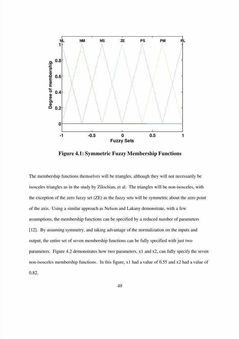
Figure 4.1: Symmetric Fuzzy Membership Functions
The membership functions themselves will be triangles, although they will not necessarily be
isosceles triangles as in the study by Zilochian, et al. The triangles will be non-isosceles, with
the exception of the zero fuzzy set (ZE) as the fuzzy sets will be symmetric about the zero point
of the axis. Using a similar approach as Nelson and Lakany demonstrate, with a few
assumptions, the membership functions can be specified by a reduced number of parameters
[12]. By assuming symmetry, and taking advantage of the normalization on the inputs and
output, the entire set of seven membership functions can be fully specified with just two
parameters. Figure 4.2 demonstrates how two parameters, x1 and x2, can fully specify the seven
non-isosceles membership functions. In this figure, x1 had a value of 0.55 and x2 had a value of
0.82.
8/6/2019 Vick Andrew
http://slidepdf.com/reader/full/vick-andrew 57/99
8/6/2019 Vick Andrew
http://slidepdf.com/reader/full/vick-andrew 58/99
51
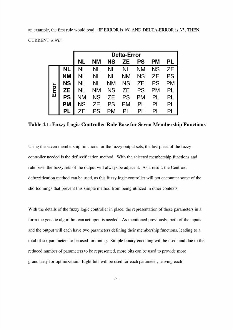
an example, the first rule would read, “IF ERROR is NL AND DELTA-ERROR is NL, THEN
CURRENT is NL”.
Table 4.1: Fuzzy Logic Controller Rule Base for Seven Membership Functions
Using the seven membership functions for the fuzzy output sets, the last piece of the fuzzy
controller needed is the defuzzification method. With the selected membership functions and
rule base, the fuzzy sets of the output will always be adjacent. As a result, the Centroid
defuzzification method can be used, as this fuzzy logic controller will not encounter some of the
shortcomings that prevent this simple method from being utilized in other contexts.
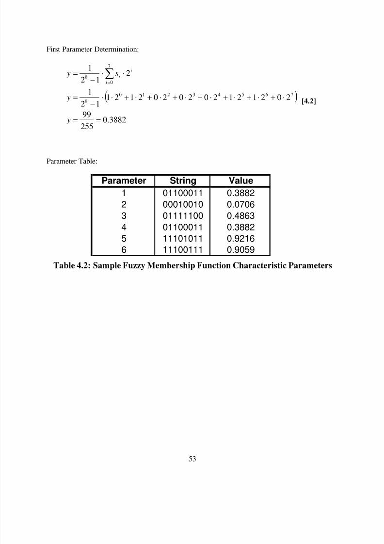
With the details of the fuzzy logic controller in place, the representation of these parameters in a
form the genetic algorithm can act upon is needed. As mentioned previously, both of the inputs
and the output will each have two parameters defining their membership functions, leading to a
total of six parameters to be used for tuning. Simple binary encoding will be used, and due to the
reduced number of parameters to be represented, more bits can be used to provide more
granularity for optimization. Eight bits will be used for each parameter, leaving each
NL NM NS ZE PS PM PL
NL NL NL NL NL NM NS ZE
NM NL NL NL NM NS ZE PS
NS NL NL NM NS ZE PS PM
ZE NL NM NS ZE PS PM PL
PS NM NS ZE PS PM PL PL
PM NS ZE PS PM PL PL PL
PL ZE PS PM PL PL PL PL
Delta-Error
E r r o r

8/6/2019 Vick Andrew
http://slidepdf.com/reader/full/vick-andrew 59/99
8/6/2019 Vick Andrew
http://slidepdf.com/reader/full/vick-andrew 60/99
53
First Parameter Determination:
( )
0.3882255
99
202121202020212112
1
212
1
765432108
7
08
==
⋅+⋅+⋅+⋅+⋅+⋅+⋅+⋅⋅−
=
⋅⋅−
= ∑=
y
y
s yi
i
i
[4.2]
Parameter Table:
Table 4.2: Sample Fuzzy Membership Function Characteristic Parameters
Parameter String Value
1 01100011 0.38822 00010010 0.0706
3 01111100 0.4863
4 01100011 0.3882
5 11101011 0.9216
6 11100111 0.9059
8/6/2019 Vick Andrew
http://slidepdf.com/reader/full/vick-andrew 61/99
54
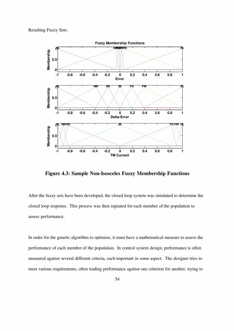
Resulting Fuzzy Sets:
-1 -0.8 -0.6 -0.4 -0.2 0 0.2 0.4 0.6 0.8 1
0
0.5
1
Error
M e m b e r s h i p
NL NMNSZEPSPM PL
Fuzzy Membership Functions
-1 -0.8 -0.6 -0.4 -0.2 0 0.2 0.4 0.6 0.8 1
0
0.5
1
Delta-Error
M e m b e r s h i p
NL NM NS ZE PS PM PL
-1 -0.8 -0.6 -0.4 -0.2 0 0.2 0.4 0.6 0.8 1
0
0.5
1
TM Current
M e m b e r s h i p
NL NM NS ZE PS PM PL
Figure 4.3: Sample Non-Isosceles Fuzzy Membership Functions
After the fuzzy sets have been developed, the closed loop system was simulated to determine the
closed loop response. This process was then repeated for each member of the population to
assess performance.
In order for the genetic algorithm to optimize, it must have a mathematical measure to assess the
performance of each member of the population. In control system design, performance is often
measured against several different criteria, each important in some aspect. The designer tries to
meet various requirements, often trading performance against one criterion for another, trying to

8/6/2019 Vick Andrew
http://slidepdf.com/reader/full/vick-andrew 62/99
55
develop an overall balanced design. This system isn’t any different, requiring a design that tries
to maximize performance against several different criteria.
In this study, the performance of the closed loop system to a step input will be assessed using an
aggregate of the classical measures of rise time (Trise), settling time (Tset - 2%), percent
overshoot (%OS), and percent steady state error (%SSE). It is necessary to combine these
measures into a simple, comprehensive form on which the genetic algorithm can optimize. For
this study they will be summed, but first they need to be non-dimensionalized in some manner
and placed on the same order of magnitude. For this task, each of the classical measures will be
divided by the respective performance measure of a fuzzy logic controller with identically
shaped isosceles triangles, resulting in a percent comparison to this baseline configuration. The
sum will then be utilized by the genetic algorithm for optimization.
It is common practice to use these parameters in the design process as measures of controller
performance, but often times some measures are more important overall than others. In this
study, in addition to normalization, these parameters will have weightings applied within the
fitness function to try to reflect priorities in the design with respect to these parameters.
In this design, it was determined that steady state error was the most important of these
measures, as accurate fuel control is vital to gas turbine performance. Without accurate fuel
control, the engine may lose efficiency or violate operating constraints, negatively impacting

8/6/2019 Vick Andrew
http://slidepdf.com/reader/full/vick-andrew 63/99

8/6/2019 Vick Andrew
http://slidepdf.com/reader/full/vick-andrew 64/99
57
f F
Wsum
WsumOS
OS
Trise
Trise
Tset
Tset
SSE
SSE f
blblblbl
/ 1
81124
/ )%
%*2
%
%*4(
=
=+++=
+++=
[4.3]
The population for the genetic algorithm will consist of 10 members, each represented with a 48
bit binary string. This number was chosen to give opportunities for optimization but try to limit
the computation of each iteration. The genetic algorithm will run through 200 iterations for each
run. With any genetic algorithm, premature convergence has the potential to hinder some
optimization if an early candidate performs extremely well compared to the other candidates. To
try to alleviate this shortcoming, this study will perform multiple runs of the genetic algorithm,
and the best solution overall will be chosen. The initial population for each trial will be
developed at random, each bit having equal opportunity of being a 0 or 1. With each initial
population being chosen randomly, multiple runs will also help explore the design space.
Following closed loop simulation of each member, the fitness of each is determined. Then, the
candidates are ranked according to their fitness. Using an elitist scheme, the top 2 performers are
kept for the next population. Also, the worst performing member undergoes inversion, flipping
every bit character in the string, and is placed into the next population. The remaining members
are determined through a selection scheme and have opportunities for genetic variation to be
introduced.

8/6/2019 Vick Andrew
http://slidepdf.com/reader/full/vick-andrew 65/99
58
The remaining members of the next population are selected at random from the current
population, with a probability proportional to their fitness. The fitness of each member is
divided by the fitness sum across all members; yielding the percent chance that member is
selected for the next population. This can be thought of as the roulette wheel approach,
discussed in section 2.3.
After the members of the population have been determined, these members undergo genetic
variation, crossovers and mutations. This scheme will include both one and two-point
crossovers. A design parameter of the genetic algorithm is the rates for these crossovers. The
overall chance of a member undergoing a crossover is set at 0.8, of which 2/3 will be one-point
crossovers and two-point crossovers will be performed on the residual. Using an elitist scheme
enables a high crossover rate, as the best performing candidates are already preserved. The goal
of crossovers is to try to recombine pieces of existing members to form new members, which
may be better suited for the controller.
Following crossovers, the population (excluding elites and inverts) is subjected to mutation.
Again, the mutation rate is a design parameter for the algorithm developer, and in this case was
chosen as 0.02. This means that each bit in each chromosome string has a 2% chance of being
inverted. Multiple mutations can occur within the same string, or some may be left without any
alteration. Mutations are a way of trying to develop new or unexplored genetic material, which
may move closer to an optimized solution.

8/6/2019 Vick Andrew
http://slidepdf.com/reader/full/vick-andrew 66/99
59
Once the successive population has been selected and has had opportunities for genetic variation
to be introduced, it is ready for the next iteration of the genetic algorithm. The members of the
new population go through the same process, having their fitness determined from closed loop
controller performance, determining the best and worst performers, and determining the makeup
of the next population. This process is repeated for each iteration, and over time, a more
optimized solution than the original population should be produced.

8/6/2019 Vick Andrew
http://slidepdf.com/reader/full/vick-andrew 67/99
60
Chapter 5
Controller Selection and Closed Loop Analysis
With the binary representation, population selection, and genetic variation rates in place, the
genetic algorithm is ready to be run. For this study, the algorithm was run five different times,
each with a different random initial population, and the best performing candidate and its
corresponding fitness rating was saved from each run. In the end, the member of the population
with the best overall fitness rating was selected for the final controller design.
A comparison of the best performer from each of the runs is shown below in Table 5.1. This
table shows the chromosome string from each candidate, the results for the performance
measures, and the corresponding fitness value.
Table 5.1: Genetic Algorithm Performance Comparison
In general, the performance of each of the runs is pretty comparable. In fact, runs 3 and 5
produced the exact same solution for the best performing candidate. The solution found from the
first run had the best overall performance, with a fitness rating of 13.01. Even though the other
solutions did not quite result in the same level of performance, they all still demonstrated
Run Chromosome Trise Tset %OS %SSE Fitness
1 10010110000000100001000000011000001000111111111 0.250 0.363 0.0002 0.0003 13.01
2 00111011000010110000110000000000011000101110101 0.263 0.363 0.0092 0.0092 12.07
3 00111101001010010010000100000101000110001110110 0.288 0.413 0.0045 0.0045 11.11
4 01101110001000100000110000101101000001011111010 0.288 0.413 0.0014 0.0008 11.35
5 00111101001010010010000100000101000110001110110 0.288 0.413 0.0045 0.0045 11.11
8/6/2019 Vick Andrew
http://slidepdf.com/reader/full/vick-andrew 68/99
61
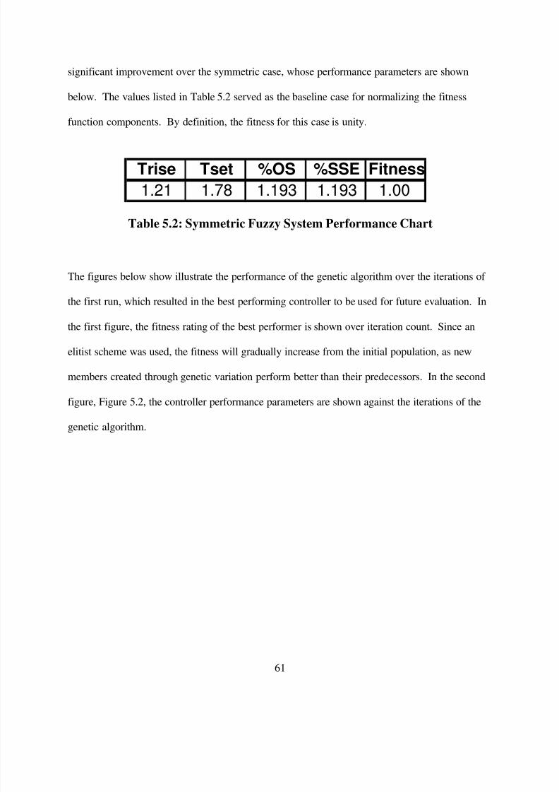
significant improvement over the symmetric case, whose performance parameters are shown
below. The values listed in Table 5.2 served as the baseline case for normalizing the fitness
function components. By definition, the fitness for this case is unity.
Table 5.2: Symmetric Fuzzy System Performance Chart
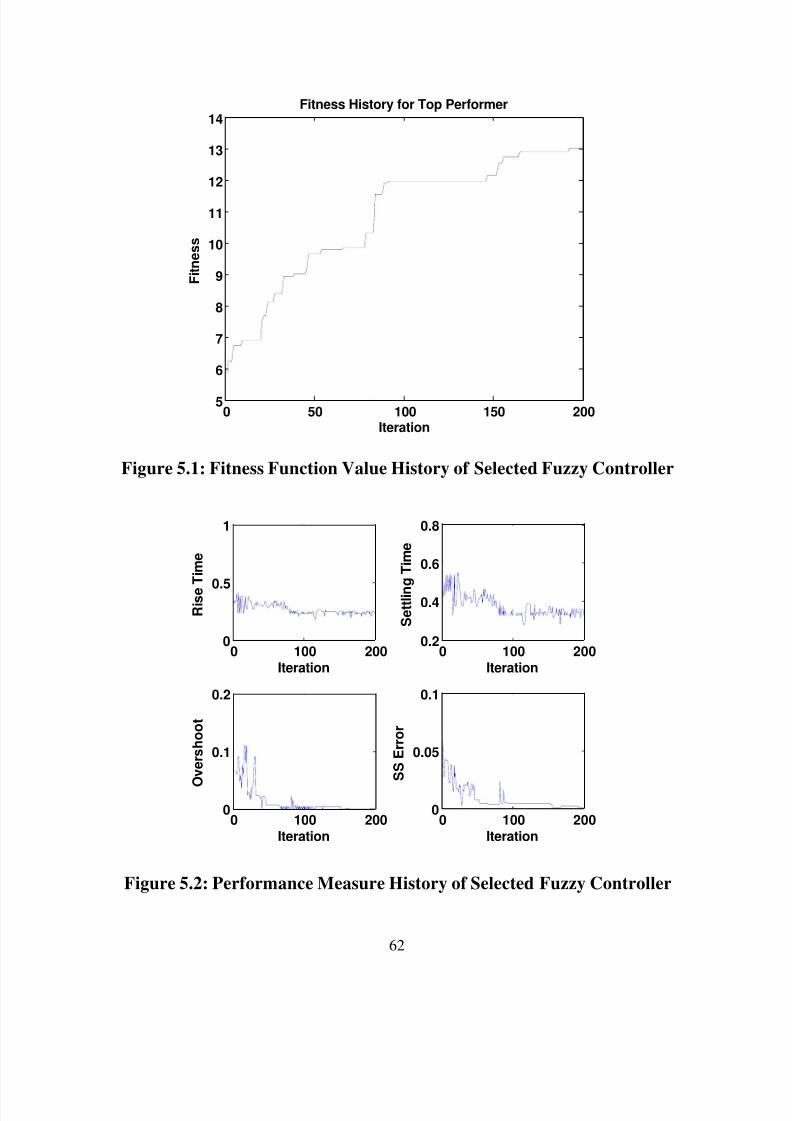
The figures below show illustrate the performance of the genetic algorithm over the iterations of
the first run, which resulted in the best performing controller to be used for future evaluation. In
the first figure, the fitness rating of the best performer is shown over iteration count. Since an
elitist scheme was used, the fitness will gradually increase from the initial population, as new
members created through genetic variation perform better than their predecessors. In the second
figure, Figure 5.2, the controller performance parameters are shown against the iterations of the
genetic algorithm.
Trise Tset %OS %SSE Fitness
1.21 1.78 1.193 1.193 1.00
8/6/2019 Vick Andrew
http://slidepdf.com/reader/full/vick-andrew 69/99
62
0 50 100 150 2005
6
7
8
9
10
11
12
13
14Fitness History for Top Performer
Iteration
F i t n e s s
Figure 5.1: Fitness Function Value History of Selected Fuzzy Controller
0 100 2000
0.5
1
R i s e
T i m e
Iteration0 100 200
0.2
0.4
0.6
0.8
S e t t l i n
g T i m e
Iteration
0 100 2000
0.1
0.2
O
v e r s h o o t
Iteration0 100 200
0
0.05
0.1
S S E r r o r
Iteration
Figure 5.2: Performance Measure History of Selected Fuzzy Controller
8/6/2019 Vick Andrew
http://slidepdf.com/reader/full/vick-andrew 70/99
63
Using an elitist scheme ensures the best performer is kept from one iteration to the next, however
since overall performance is based on a weighted combination of four individual performance
parameters, it is possible to see some increases in these figures in the general downward trend.
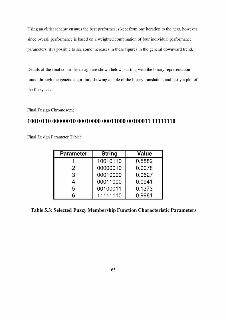
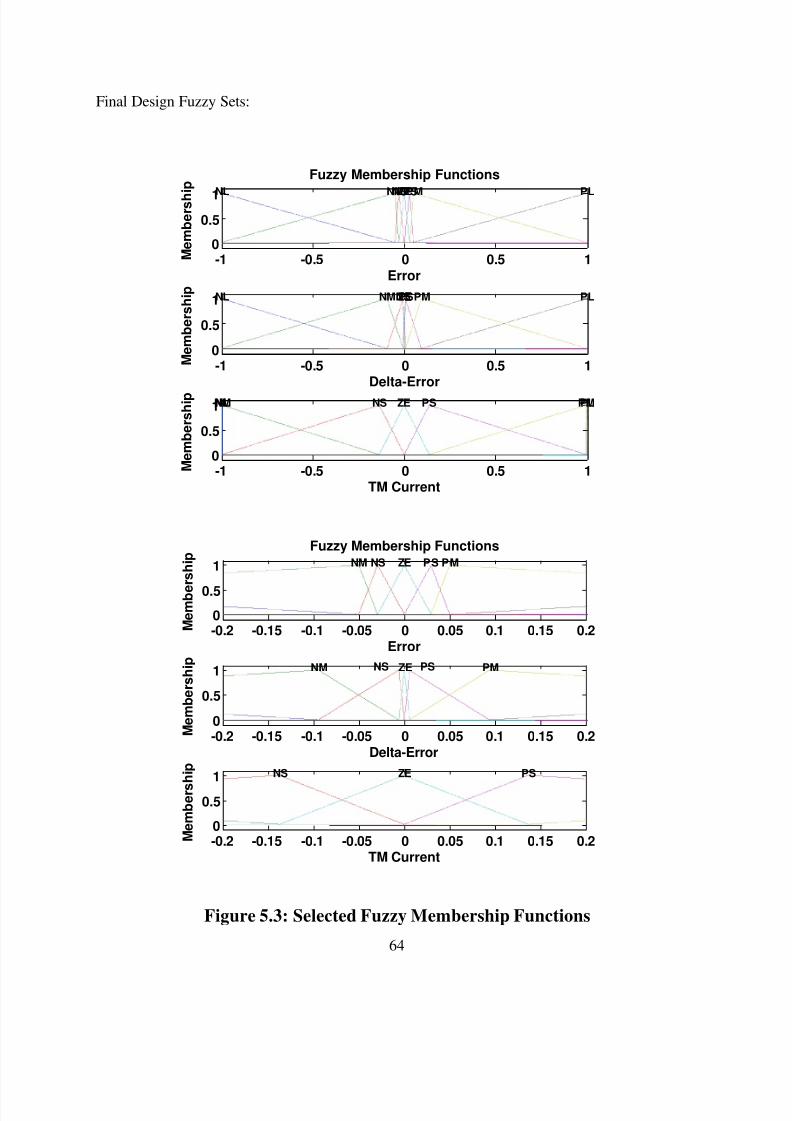
Details of the final controller design are shown below, starting with the binary representation
found through the genetic algorithm, showing a table of the binary translation, and lastly a plot of
the fuzzy sets.
Final Design Chromosome:
10010110 00000010 00010000 00011000 00100011 11111110
Final Design Parameter Table:
Table 5.3: Selected Fuzzy Membership Function Characteristic Parameters
Parameter String Value
1 10010110 0.5882
2 00000010 0.00783 00010000 0.0627
4 00011000 0.0941
5 00100011 0.1373
6 11111110 0.9961
8/6/2019 Vick Andrew
http://slidepdf.com/reader/full/vick-andrew 71/99
64
Final Design Fuzzy Sets:
-1 -0.5 0 0.5 10
0.5
1
Error
M e m b e r s h
i p
NL NMNSZEPSPM PL
Fuzzy Membership Functions
-1 -0.5 0 0.5 10
0.5
1
Delta-Error
M e m b e r s h i p
NL NMNSZEPSPM PL
-1 -0.5 0 0.5 10
0.5
1
TM Current
M e m b e r s h i p NLNM NS ZE PS PMPL
-0.2 -0.15 -0.1 -0.05 0 0.05 0.1 0.15 0.20
0.5
1
Error
M e m b e
r s h i p
NM NS ZE PS PM
Fuzzy Membership Functions
-0.2 -0.15 -0.1 -0.05 0 0.05 0.1 0.15 0.20
0.5
1
Delta-Error
M e m b e r s h i p
NM NS ZE PS PM
-0.2 -0.15 -0.1 -0.05 0 0.05 0.1 0.15 0.20
0.5
1
TM Current
M e m b e r s
h i p
NS ZE PS
Figure 5.3: Selected Fuzzy Membership Functions

8/6/2019 Vick Andrew
http://slidepdf.com/reader/full/vick-andrew 72/99
8/6/2019 Vick Andrew
http://slidepdf.com/reader/full/vick-andrew 73/99
66
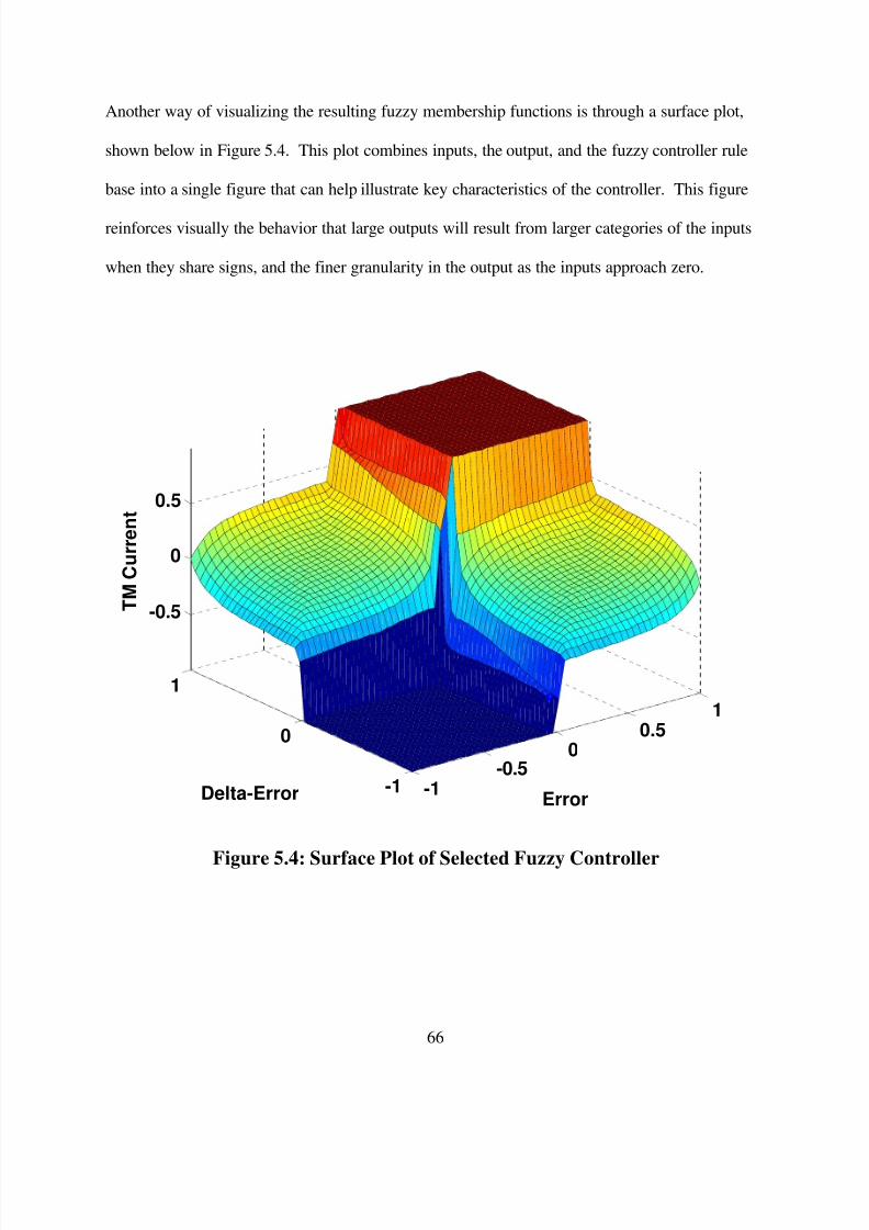
Another way of visualizing the resulting fuzzy membership functions is through a surface plot,
shown below in Figure 5.4. This plot combines inputs, the output, and the fuzzy controller rule
base into a single figure that can help illustrate key characteristics of the controller. This figure
reinforces visually the behavior that large outputs will result from larger categories of the inputs
when they share signs, and the finer granularity in the output as the inputs approach zero.
-1-0.5
00.5
1
-1
0
1
-0.5
0
0.5
ErrorDelta-Error
T M
C u r r e n t
Figure 5.4: Surface Plot of Selected Fuzzy Controller
8/6/2019 Vick Andrew
http://slidepdf.com/reader/full/vick-andrew 74/99
67
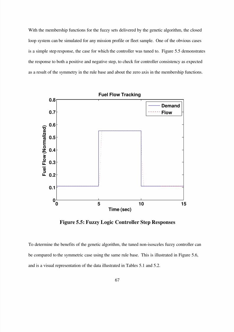
With the membership functions for the fuzzy sets delivered by the genetic algorithm, the closed
loop system can be simulated for any mission profile or fleet sample. One of the obvious cases
is a simple step response, the case for which the controller was tuned to. Figure 5.5 demonstrates
the response to both a positive and negative step, to check for controller consistency as expected
as a result of the symmetry in the rule base and about the zero axis in the membership functions.
0 5 10 150
0.1
0.2
0.3
0.4
0.5
0.6
0.7
0.8Fuel Flow Tracking
Time (sec)
F
u e l F l o w ( N o r m a l i z e d )
Demand
Flow
Figure 5.5: Fuzzy Logic Controller Step Responses
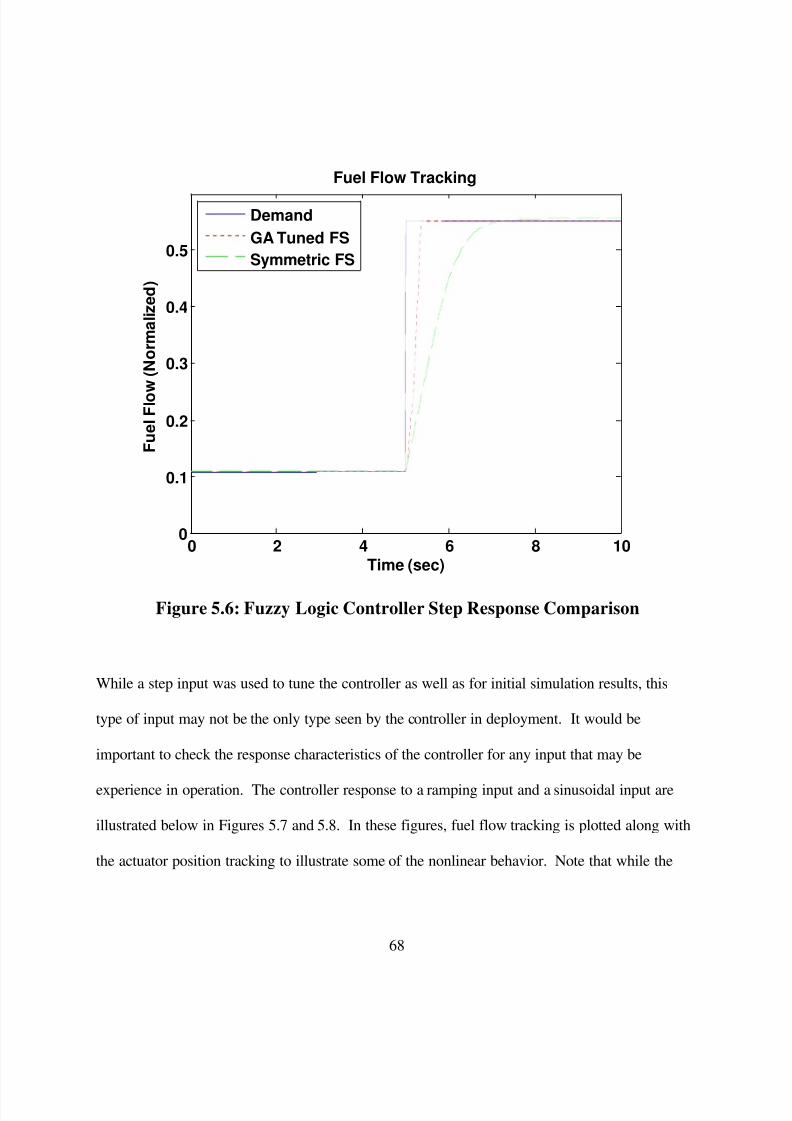
To determine the benefits of the genetic algorithm, the tuned non-isosceles fuzzy controller can
be compared to the symmetric case using the same rule base. This is illustrated in Figure 5.6,
and is a visual representation of the data illustrated in Tables 5.1 and 5.2.
8/6/2019 Vick Andrew
http://slidepdf.com/reader/full/vick-andrew 75/99
8/6/2019 Vick Andrew
http://slidepdf.com/reader/full/vick-andrew 76/99
69
controller was not tuned for these cases, the controller still performs very well to both inputs,
showing good tracking behavior to both sets of input types.
0 5 10 150
0.2
0.4
0.6
0.8
1
Fuel Flow Tracking
F
u e l F l o w ( N o r m )
Demand
Flow
0 5 10 150.4
0.6
0.8
1
1.2Actuator Position Tracking
Time (sec)
A c t u a t o r P o
s i t i o n ( N o r m )
Demand
Position
Figure 5.7: Fuzzy Logic Controller Ramp Response
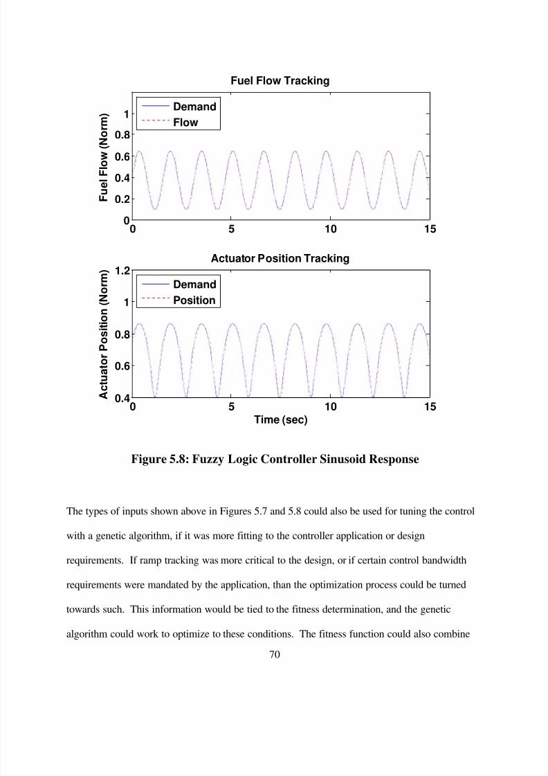
8/6/2019 Vick Andrew
http://slidepdf.com/reader/full/vick-andrew 77/99

8/6/2019 Vick Andrew
http://slidepdf.com/reader/full/vick-andrew 78/99
71
performance against various criteria or requirements to drive towards a balanced design in a
competing space.
8/6/2019 Vick Andrew
http://slidepdf.com/reader/full/vick-andrew 79/99
72
Chapter 6
Controller Robustness Analysis
With the controller design selected in Chapter 5, the next step is to gauge the performance
robustness of the closed loop system. This study will use the stochastic robustness analysis
demonstrated by Stengel and others in many applications characterized by some level of
uncertainty. As discussed in Chapter 2.4, this analysis involves a Monte Carlo simulation of the
closed loop system, considering variation within the components or across operating conditions.
This study will consider variation within the modeled hardware components, representing part-
to-part variation within a fleet or perhaps component degradation over time. Component
characteristics with uncertainty considered in this study are summarized in Table 6.1 below.
Table 6.1: Summary of Stochastic Parameters in Closed Loop System
Electro-Hydraulic Servo Valve
Null Current
Hysteresis
Current Time Constant
Flow Time Constant
Flow Gain
Linerar Variable Displacement Transducer
Natural FrequencyDamping

8/6/2019 Vick Andrew
http://slidepdf.com/reader/full/vick-andrew 80/99
73
The uncertainty associated with each of the parameters listed in Table 6.1 will be represented by
a Gaussian distribution, with mean values and standard deviations representative of variation
within each component.
For this study, a total of 1000 closed loop simulations will be run, each using a different set or
variation parameters determined randomly from the Gaussian distributions for each uncertainty
term. The system will be simulated with a step input in fuel demand, as in the case used to tune
the controller. Each simulation will be gauged for performance against parameters discussed
above, mainly the rise and settling times, overshoot, and steady state error. The fitness function
will also be generated for each case as means to compare performance to the design case and
gauge performance across all the Monte Carlo runs.
In some cases, it may make sense for the robustness analysis to be performed on a collection of
simulation cases, such as a complete mission analysis or cases known to be challenging in terms
of performance. The selection is up to the designer, and at a minimum should be able to assess
controller performance against the design requirements.
In order to assess controller robustness, criteria needs to be developed for determining if
performance is adequate. These criteria will be selected to provide a binary determination, or
pass/fail criteria. For the purposes of this study, performance will be deemed acceptable for rise
and settling time requirements if the times are less than double those of the design case, or less
than 0.50 and 0.725 seconds respectively. In terms of overshoot, a limit of 0.5% will be used;
anything more and performance will be considered inadequate. For the steady state error limit, a
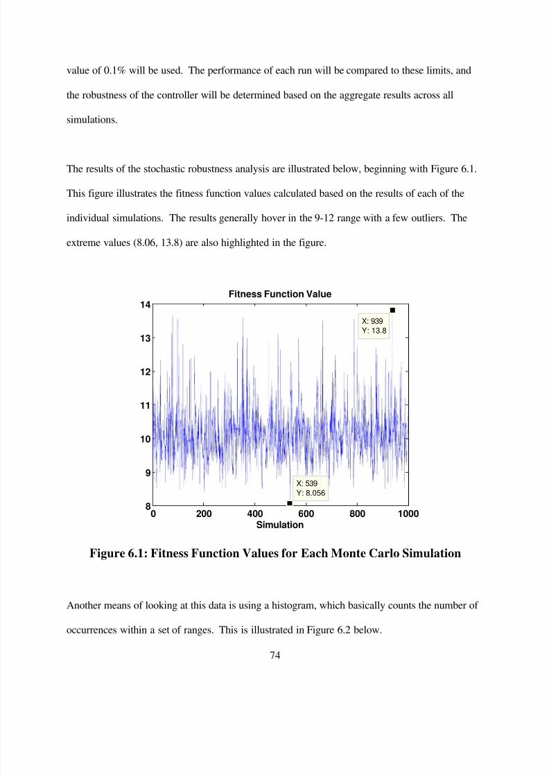
8/6/2019 Vick Andrew
http://slidepdf.com/reader/full/vick-andrew 81/99
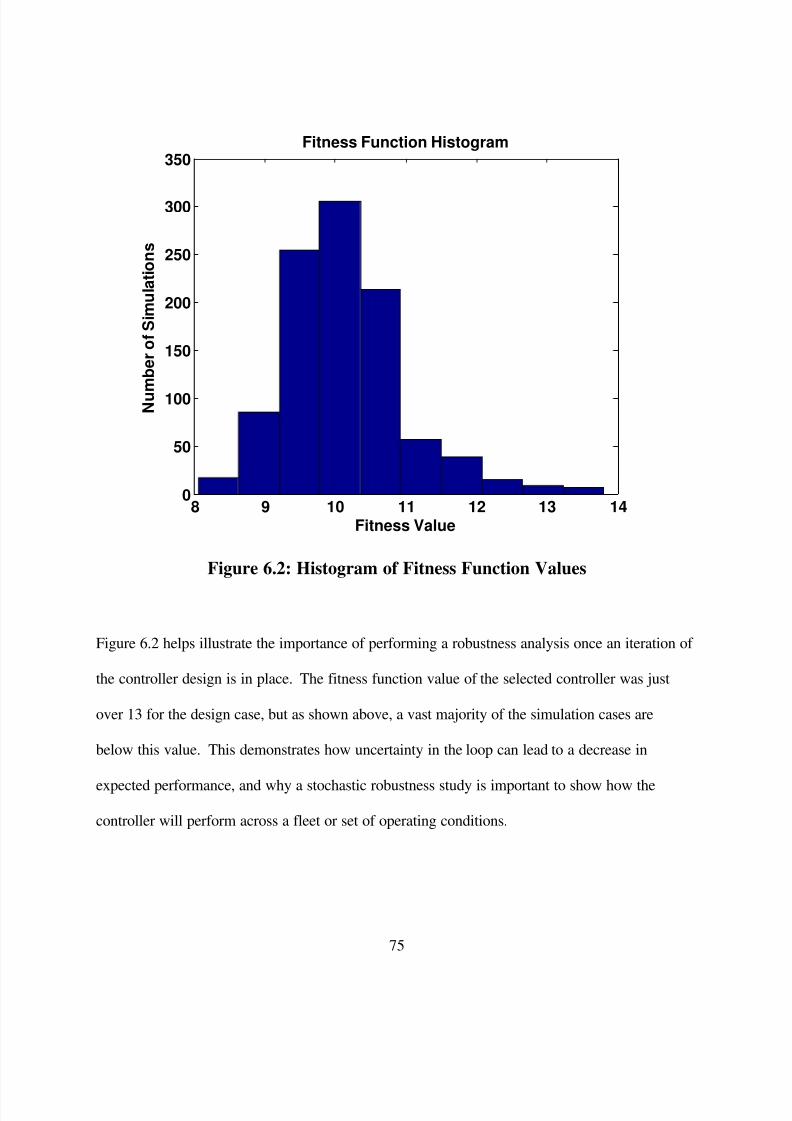
8/6/2019 Vick Andrew
http://slidepdf.com/reader/full/vick-andrew 82/99
75
8 9 10 11 12 13 140
50
100
150
200
250
300
350Fitness Function Histogram
Fitness Value
N u m b e r o f S i m u l a t i o n s
Figure 6.2: Histogram of Fitness Function Values
Figure 6.2 helps illustrate the importance of performing a robustness analysis once an iteration of
the controller design is in place. The fitness function value of the selected controller was just
over 13 for the design case, but as shown above, a vast majority of the simulation cases are
below this value. This demonstrates how uncertainty in the loop can lead to a decrease in
expected performance, and why a stochastic robustness study is important to show how the
controller will perform across a fleet or set of operating conditions.

8/6/2019 Vick Andrew
http://slidepdf.com/reader/full/vick-andrew 83/99
76
Figure 6.3, below, compares performance of the cases with the minimum and maximum fitness
function values to the base case from the original design. The figure includes both a plot of the
full response and a plot zoomed in at the top of the step to capture some of the details of the
compared cases. As shown, the differences are very slight, with the biggest differences seen in
overshot and steady state error. This figure demonstrates the robustness properties of the fuzzy
logic controller, that even in a nonlinear environment with uncertainties, the controller can
maintain a high level of performance.
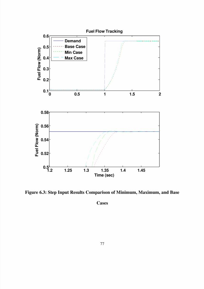
8/6/2019 Vick Andrew
http://slidepdf.com/reader/full/vick-andrew 84/99
77
0 0.5 1 1.5 20.1
0.2
0.3
0.4
0.5
0.6Fuel Flow Tracking
F u e l F l o w ( N o r m
)
Demand
Base Case
Min Case
Max Case
1.2 1.25 1.3 1.35 1.4 1.450.5
0.52
0.54
0.56
0.58
Time (sec)
F u e l F l o w ( N o r m )
Figure 6.3: Step Input Results Comparison of Minimum, Maximum, and Base
Cases
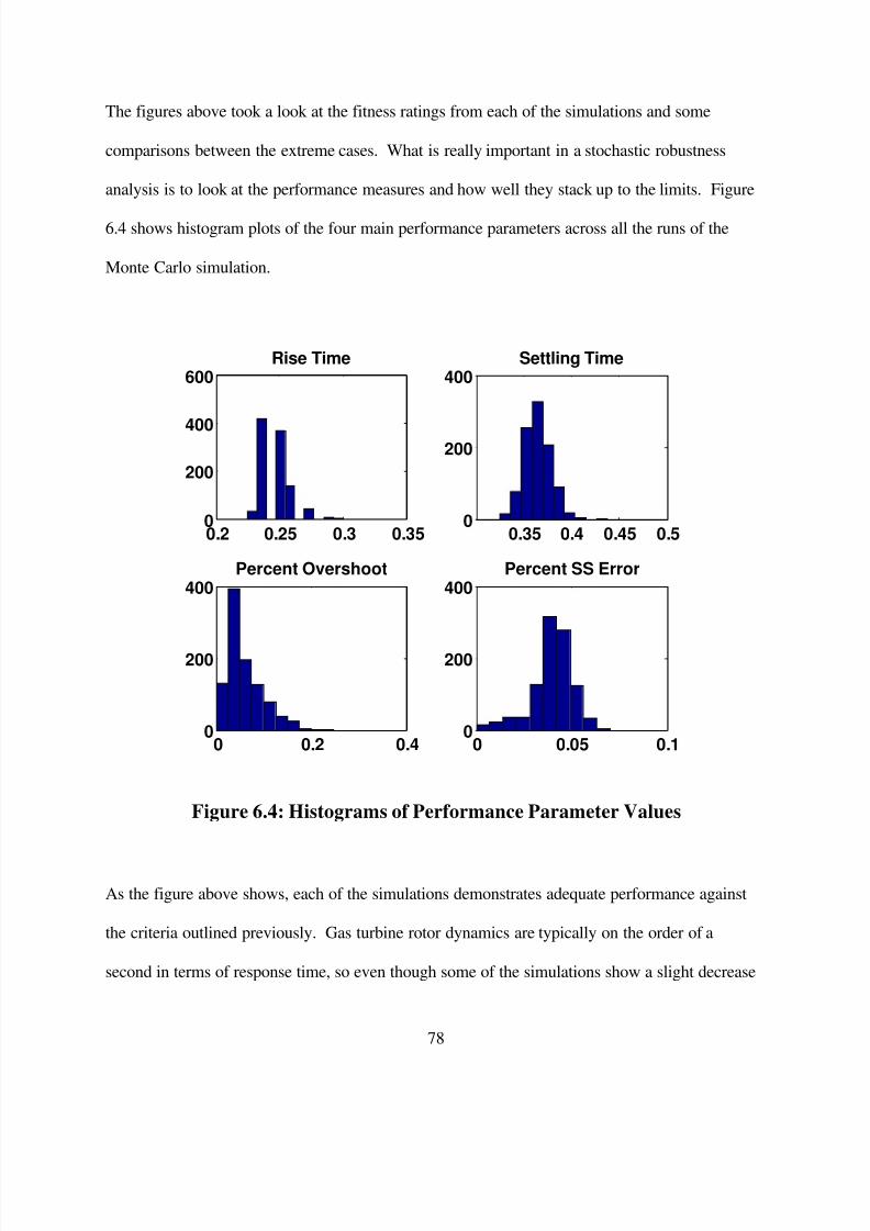
8/6/2019 Vick Andrew
http://slidepdf.com/reader/full/vick-andrew 85/99
78
The figures above took a look at the fitness ratings from each of the simulations and some
comparisons between the extreme cases. What is really important in a stochastic robustness
analysis is to look at the performance measures and how well they stack up to the limits. Figure
6.4 shows histogram plots of the four main performance parameters across all the runs of the
Monte Carlo simulation.
0.2 0.25 0.3 0.350
200
400
600Rise Time
0.35 0.4 0.45 0.50
200
400Settling Time
0 0.2 0.40
200
400Percent Overshoot
0 0.05 0.10
200
400Percent SS Error
Figure 6.4: Histograms of Performance Parameter Values
As the figure above shows, each of the simulations demonstrates adequate performance against
the criteria outlined previously. Gas turbine rotor dynamics are typically on the order of a
second in terms of response time, so even though some of the simulations show a slight decrease

8/6/2019 Vick Andrew
http://slidepdf.com/reader/full/vick-andrew 86/99
79
in performance with respect to the design case, the controller still should respond fast enough to
maintain adequate control.
It is important to note that uncertainties in a few terms of the control loop were neglected for this
study. However, these terms are known to be small in comparison to the uncertainties that were
considered, and are not expected to affect the results to a large degree. In addition, as
demonstrated below in Table 6.2, the performance parameters have margins ranging from 30-
50% to the selected limits, leaving some flexibility for these effects.
Table 6.2: Stochastic Robustness Analysis Performance Summary
Table 6.2 underscores the importance of performing a robustness analysis on a controller design.
Looking at the first row, the average fitness across the runs was just over 10, a significant drop
when compared to the design case of 13. As mentioned previously, this is a strong indicator of
how uncertainty can impact performance. Looking at the two rows for the timing measures, the
mean case did not deviate significantly from the design case. In fact, the rise time average was
actually lower than base case, albeit only by a small degree. Each of these parameters has 40 %
margin to the selected design limit.
Parameter Base Case Average Case Min Case Max Case Limit Case Margin
Fitness 13.0 10.1 8.06 13.8 N/A N/A
Rise Time (sec) 0.250 0.247 0.225 0.300 0.500 40%
Settling Time (sec) 0.363 0.363 0.325 0.438 0.726 40%
Overshoot (%) 0.0002 0.060 0.000 0.248 0.500 50%
Steady State Error (%) 0.0003 0.0397 0.0001 0.0703 0.1000 30%

8/6/2019 Vick Andrew
http://slidepdf.com/reader/full/vick-andrew 87/99

8/6/2019 Vick Andrew
http://slidepdf.com/reader/full/vick-andrew 88/99
81
Another option would be to use information from the specific performance failure cases to adjust
tolerances for the system. If the stochastic analysis represented fleet variation, than an inspection
process could be put in place to prevent hardware exhibiting those qualities from being deployed
in the field if the component was on the fringe of the Gaussian curve. The designer could also
choose to live with the performance exception, depending on the conditions and how critical to
the overall control system that simulated case represents.
As demonstrated, stochastic robustness analysis is a critical tool when evaluating controller
design in an uncertain environment. Considering manufacturing processes, component
tolerances, and operating conditions, one would be hard pressed to find a system without some
level of uncertainty. This type analysis is critical to ensuring a designer develops a robust
control system, one that will be able to meet its design objectives in foreseeable environments.

8/6/2019 Vick Andrew
http://slidepdf.com/reader/full/vick-andrew 89/99
82
Chapter 7
Conclusions and Future Research
In this study, a fuzzy logic controller was designed for a gas turbine fuel system. The design
process began with the basic structure used by Zilouchian and others in their study for a fuel
system simulation bench [35]. This study contributed the input/output definition, as well as the
rule base. Their approach utilized identically shaped isosceles triangles for the fuzzy set
definitions, which can be constraining when trying to tune the controller for improved
performance. Nelson and Lakany evaluated the use of non-isosceles triangular membership
functions for increased tuning flexibility, defined using an approach that reduces the number of
tunable parameters to a more manageable level [12]. These two studies formed the backbone of
the fuzzy logic controller utilized in this study, while a genetic algorithm was utilized in a unique
tuning approach.
The genetic algorithm was used with simple binary encoding for each of the parameters
governing the fuzzy sets for the inputs and output of the controller. Multiple runs of the genetic
algorithm, each with a unique random initial population, were employed to try to workaround the
potential for premature convergence. As Table 5.1 illustrates, each of the genetic algorithm runs
converged to a similar solution, speaking to the robustness of the algorithm itself. As the
simulation results indicate, each of the solutions demonstrated significant performance
improvements over the symmetric isosceles fuzzy set case. This stands to show that even with
the simplifications put in place to reduce the number of tuning parameters, enough flexibility
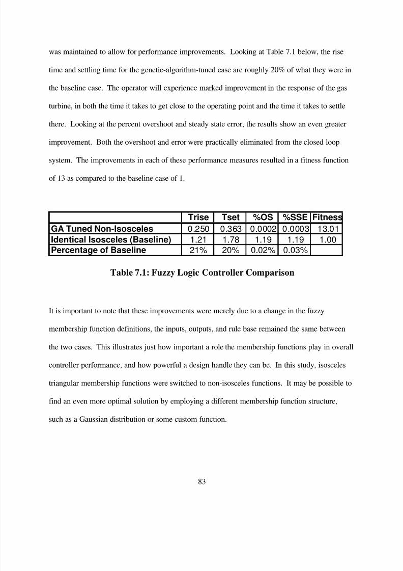
8/6/2019 Vick Andrew
http://slidepdf.com/reader/full/vick-andrew 90/99
83
was maintained to allow for performance improvements. Looking at Table 7.1 below, the rise
time and settling time for the genetic-algorithm-tuned case are roughly 20% of what they were in
the baseline case. The operator will experience marked improvement in the response of the gas
turbine, in both the time it takes to get close to the operating point and the time it takes to settle
there. Looking at the percent overshoot and steady state error, the results show an even greater
improvement. Both the overshoot and error were practically eliminated from the closed loop
system. The improvements in each of these performance measures resulted in a fitness function
of 13 as compared to the baseline case of 1.
Table 7.1: Fuzzy Logic Controller Comparison
It is important to note that these improvements were merely due to a change in the fuzzy
membership function definitions, the inputs, outputs, and rule base remained the same between
the two cases. This illustrates just how important a role the membership functions play in overall
controller performance, and how powerful a design handle they can be. In this study, isosceles
triangular membership functions were switched to non-isosceles functions. It may be possible to
find an even more optimal solution by employing a different membership function structure,
such as a Gaussian distribution or some custom function.
Trise Tset %OS %SSE Fitness
GA Tuned Non-Isosceles 0.250 0.363 0.0002 0.0003 13.01
Identical Isosceles (Baseline) 1.21 1.78 1.19 1.19 1.00Percentage of Baseline 21% 20% 0.02% 0.03%

8/6/2019 Vick Andrew
http://slidepdf.com/reader/full/vick-andrew 91/99
84
The performance of the fuzzy logic controller was improved in several measures based on the
fitness function developed in Chapter 4. The fitness function was normalized, weighted, and
inverted to yield a relation that could be maximized by the genetic algorithm, where successive
populations could be selected proportional to fitness. With the flexibility of genetic algorithms,
there are a number of different approaches that can be used. Instead of inverting the fitness
function, the algorithm could be set up to minimize the performance function if a different
population selection scheme was used. Another alternative would be to multiply the fitness
function by –1 instead of inverting, and setup the algorithm to maximize –f. Either of these
approaches would change the appearance of the fitness history shown in Figure 5.1, where the
fitness jumps up in large segments due to incremental changes in the performance characteristics
because of the inversion.
A few other design decisions were made regarding the genetic algorithm that could also
influence the results. Utilizing multiple runs for this study was designed to avoid the risk of
premature convergence. There are a few other techniques that could be explored to try to
accomplish this as well, such as using a different representation of the design parameters. The
population size for the runs was also set to 10, which is on the smaller side compared to some
genetic algorithm runs. This was done to try to balance computational iterations but still give a
chance to optimize. Of course, the population could be expanded to a much larger base, and
perhaps multiple runs wouldn’t be needed. The algorithm could have also been set up to run for
a longer number of iterations, but this study tried to strike a balance between computational time
and incrementally small improvements to the closed loop system.

8/6/2019 Vick Andrew
http://slidepdf.com/reader/full/vick-andrew 92/99
85
Inversion was a variation process introduced into the genetic algorithm, with mixed results. In
several cases, the inverted chromosome ended up performing somewhere in the middle of the
population in the subsequent generation, but only in one instance did the inverted chromosome
end up being a top performer in the next generation. This one case was early in the iteration
process, and didn’t end up being the final chromosome selected, but may have accelerated the
process to converging to the solution by introducing a string of good genetic material. One trend
to note was that this process was less effective in later iterations as the population collectively
improved overall, and inversions generally led to poorer performance in successive iterations.
With a controller design in place, a stochastic robustness analysis was performed using several
simulations of the closed loop system to determine how the controller would behave in a range of
environments resulting from uncertainty in the closed loop system. This type of analysis can be
more useful than classical measures such as gain and phase margins, which can be
misrepresentative in stochastic environments. This analysis only used a single test case for
illustrative purposes, but could be expanded for a more complete mission analysis. The results
of the analysis here showed the controller performed adequately in each simulation of the Monte
Carlo analysis, with little degradation when variation was considered. This illustrates the
inherent robustness properties of fuzzy logic controllers, and their abilities to operate in varying
environments.
The fuzzy logic controller was shown to be a viable option for the given environment, and the
genetic algorithm proved to be very beneficial in the tuning process. The algorithm did take a bit
of computational time considering each iteration of each run, however once a streamlined

8/6/2019 Vick Andrew
http://slidepdf.com/reader/full/vick-andrew 93/99

8/6/2019 Vick Andrew
http://slidepdf.com/reader/full/vick-andrew 94/99
87
References
[1] K. H. Ang, G. C. Y. Chong, and Y. Li (2007). “PID Control System Analysis, Design,
and Technology,” IEEE Transactions on Control Systems Technology, vol. 12, no. 4,
pp. 559-576.
[2] M. Araki, "PID Control (2009). “Control Systems, Robotics, and Automation, vol. II,
EOLSS Publishers Co Ltd.
[3] P. P. Bonissone and K. H. Chiang (1993). “Fuzzy Logic Controllers: from
Development to Deployment,” 1993 IEEE International Conference on Neural
Networks, vol. 2, 1993.
[4] P. P. Bonissone et al. (1995). “Industrial Applications of Fuzzy Logic at General
Electric,” Proceedings of The IEEE, vol. 83, no. 3, pp. 450-465.
[5] D. E. Bossert and K. Cohen (2002). “PID and Fuzzy Logic Pitch Attitude Hold Systems
for a Fighter Jet,” AIAA Guidance, Navigation, and Control Conference and Exhibit ,
August 2002.
[6] K. Cohen, T. Weller, and J. Z. Ben Asher (2001). “Control of Linear Second-Order
Systems by Fuzzy Logic-Based Algorithm,” Journal of Guidance, Control, and
Dynamics, vol. 24, no. 3, pp. 494-501.
8/6/2019 Vick Andrew
http://slidepdf.com/reader/full/vick-andrew 95/99
88
[7] O. Cordon, F. Herrera, F. Hoffmann, and L. Magdalena (2001). Genetic Fuzzy Systems:
Evolutionary Tuning and Learning of Fuzzy Knowledge Bases, New Jersey, World
Scientific, 2001.
[8] J. H. Holland (1975). Adaptation in Natural and Artificial Systems, Michigan,
University of Michigan Press, 1975.
[9] E. Khan and S. Rahman (1995). “Fuzzy Logic Gets a Boost From Neural Nets,”
Electronic Design, June 1995, pp. 128-132.
[10] E. H. Mamdani (1977). “Application of Fuzzy Logic to Approximate Reasoning Using
Linguistic Synthesis,” IEEE Transactions on Computers, vol. 26, no. 12, pp. 1182-
1191.
[11] J. M. Mendel (1995). “Fuzzy Logic Systems for Engineering: A Tutorial,” Proceedings
of The IEEE, vol. 83, no. 3, pp. 345-377.
[12] G. M. Nelson and H. Lakany (2007). “An Investigation Into the Application of Fuzzy
Logic Control to Industrial Gas Turbines,” Journal of Engineering for Gas Turbines
and Power, Transactions of the ASME , vol. 129, pp. 1138-1142.

8/6/2019 Vick Andrew
http://slidepdf.com/reader/full/vick-andrew 96/99
89
[13] H. O. Nyongesa (1998). “Enhancing Neural Control Systems by Fuzzy Logic and
Evolutionary Reinforcement,” Neural Computing & Applications, vol. 7, no. 2, pp.
121-130.
[14] B. Paiewonsky (1965). “Optimal Control: A Review of Theory and Practice,” AIAA
Journal, vol. 3, no. 11, pp. 1985-2006.
[15] T. R. D. Prakash and N. K. Nair (2007). “A Robust Control Strategy for UPFC to
Improve Transient Stability Using Fuzzy Bang-Bang Control,” International
Conference on Computational Intelligence and Multimedia Applications, 2007, pp.
352-356.
[16] L. Radziszewski and M. Kekez (2009). “Application of a genetic-fuzzy system to diesel
engine pressure modeling,” The International Journal of Advanced Manufacturing
Technology, vol. 46, no. 1-4, pp. 1-9.
[17] L. R. Ray and R. F. Stengel (1991). “Application of Stochastic Robustness to Aircraft
Control Systems,” Journal of Guidance, Control, and Dynamics, vol. 14, no. 6, pp.
1251-1259.
[18] L. R. Ray and R. F. Stengel (1993). “Computer-Sided Analysis of Linear Control
System Robustness,” Mechatronics, vol. 3, no. 1, pp. 119-124.

8/6/2019 Vick Andrew
http://slidepdf.com/reader/full/vick-andrew 97/99
8/6/2019 Vick Andrew
http://slidepdf.com/reader/full/vick-andrew 98/99
91
[26] R. F. Stengel, L. R. Ray, and C. I. Marrison (1993). “Probabilistic Evaluation of
Control System Robustness,’ Institute for Mathematics and Its Applications Preprint
Series, #1094.
[27] D. E. Thomas and B. Armstong-Helouvry (1995). “Fuzzy Logic Control – A
Taxonomy of Demonstrated Benefits,” Proceedings of The IEEE, vol. 83, no. 3, pp.
407-421.
[28] A. Vick and K. Cohen (2009). “Longitudinal Stability Augmentation using a Fuzzy
Logic based PID Controller,” North American Fuzzy Information Processing Society
Annual Conference, June 2009.
[29] Q. Wang and R. F. Stengel (2002). “Robust Control of Nonlinear Systems with
Parametric Uncertainty,” Automatica, vol. 38, no. 9, pp. 1591-1599.
[30] Q. Wang and R. F. Stengel (2005). “Robust Nonlinear Flight Control of a High-
Performance Aircraft,” IEEE Transactions on Control Systems Technology, vol. 13, no.
1, pp. 15-26.
[31] K. H. You and E. B. Lee (2000). “Robust, Near Time-Optimal Control of Nonlinear
Second Order Systems with Model Uncertainty,” Proceedings of the 2000 IEEE,
International Conference on Control Applications, pp. 232-236.

8/6/2019 Vick Andrew
http://slidepdf.com/reader/full/vick-andrew 99/99
[32] W. You, H. Chen, and X. He (2010). “Tracking Control Research of High-Order
Flexible Structures on the H-Infinity Control Method,” 2nd
International Conference on
Advanced Computer Control (ICACC), vol. 5, pp. 111-115.
[33] L. A. Zadeh (1965). “Fuzzy Sets,” Information and Control, vol. 8, no. 3, pp. 338-353.
[34] L. A. Zadeh (1973). “Outline of a New Approach to the Analysis of Complex Systems
and Decision Processes,” IEEE Transactions on Systems, Man, and Cybernetics, vol.
SMC-3, no. 1, 28-44.
[35] A. Zilouchian, M. Juliano, T. Healy, and J. Davis (2000). “Design of a Fuzzy Logic
Controller for a Jet Engine Fuel System,” Control Engineering Practice, vol. 8, no. 8,
pp. 873-883.