Versión impresa ISSN: 0716-7334 Versión electrónica ISSN: …economia.uc.cl/docs/ref_04.pdf · See Alejandro Silva de la Fuente in Semana del Salitre Abril 1926, p.472 3 General

Versión impresa ISSN: 0716-7334Versión electrónica ISSN: 0717-7593

PONTIFICIA UNIVERSIDAD CATOLICA DE CHILEINSTITUTO DE ECONOMIA

Oficina de PublicacionesCasilla 76, Correo 17, Santiagowww.economia.puc.cl

EXPORT TARIFF, WELFARE AND PUBLICFINANCE: NITRATES FROM 1880 TO 1930

Rolf Lüders* **

Gert Wagner

Documento de Trabajo Nº 241

Santiago, Mayo 2003

*Rolf Lüders is Professor at the Diego Portales University in Santiago; Gert Wagner is at the Institute ofEconomics, Catholic University of Chile. Authors acknowledge financial support from the Academic Vice-rectoryof the Catholic University. Our gratitude to José Díaz for his contributions to this paper. We acknowledgecomments to an earlier version from Dominique Hachette, Ronald Fischer, Benjamin Mira, Gerardo Martinez,Fernando Ossa, Salvador Valdes, Luis Felipe Lagos and Marcus Cobb.**The paper is part of a broader investigation aiming at the understanding of Chile’s republican growth process.

INDEX

ABSTRACT 1

1. PROTECTIONISM AND THE COST OF PUBLIC REVENUE 4

2. CHILEAN NITRATES: STYLIZED FACTS 6

3. CHILE'S NITRATE MONOPOLY POWER AND THE EXPORT TAX:FIRST PERHAPS TOO LITTLE AND LATER TOO MUCH? 93.1. Conceptual framework 93.2. Estimation and data 133.3. Results 16

4. PRIVATE PARTICIPATION IN MONOPOLY RENTS. DID IT EXIST? 184.1. Private participation in the one stage monopoly context? 184.2. Second stage monopoly? 21

5. WELFARE IMPLICATIONS: A CLOSER LOOK 22

6. FINAL REMARKS 26

REFERENCES 32

APPENDIX 35TABLE A 1 35TABLE A2 36TABLE A3 37TABLE A4 38GRAPH A1 39GRAPH A2 39GRAPH A3 40GRAPH A4 40GRAPH A5 41GRAPH A6 41GRAPH A7 42GRAPH A8 42

ABSTRACT

The traditional exception to the welfare reducing character of protectionism is based on

the optimum tariff argument. If in addition the market power can be traced back to

control of a necessary, cero substitution natural resource type input, then the

corresponding trade tax and the shadow price of the resource are on common ground,

eventually the former is also an instrument for charging the latter. In the political

economy context such an export tax is also a device for nationalizing the income stream

the scenario promises; but also, once this revenue takes over a significant fraction of

fiscal income the country’s Treasury may turn into a conservative force impeding tax

innovations dictated by dwindling monopoly power. Specially so if government comes to

display an agency type of behavior and the revenue reductions to be derived from the

adaptation of the tariff to changing demand conditions concentrate in the present,

meanwhile expected benefits of such an action extend into the future.

Based on a simple analytical framework and exploring the issue with a set of

simulations, the optimality of the export tax on nitrates is evaluated for its complete

lifespan extending over half a century. Its nil capacity for adapting to changing

conditions is then interpreted in terms of the assumed incentive structure of

governments, but recognizing the inherent difficulties in predicting future market power

and therefore of tax design.

In the 1870th in face of the rapidly expanding international demand for nitrates,

concentration in its southern province of a high proportion of world’s total natural

deposits and thirdly underdeveloped technology in artificially produced nitrate, Peruvian

government puts into practice a set of policies aimed at capturing potential monopoly

rents to be derived from this situation.

To meet the challenge Peruvian nitrate industry was nationalized financing

future payment with specially designed certificates. Since geographic concentration of

deposits did not coincided completely with its own jurisdictional area, it additionally

bought establishments located in Bolivian provinces, also obtaining from its government

an agreement restricting further licensing of nitrate land. These measures plus public

2 EXPORT TARIFF, WELFARE AND PUBLIC FINANCE

control over access to nitrate mining lands in its own region should have given Peru

access to sizable profits, but it was too late.

The Pacific War started in 1879 when the Bolivian government intended to

apply a special tax on the only nitrate producing establishment not under some kind of

Peruvian regulation, a firm owned by Chileans. In the early 1880 and once authority

over the nitrate region was completed the Chilean government faced the same

opportunity, that is appropriation of rents stemming from controlled exploitation of the

natural resource.1

The government had a clear advantage in its claim. It not only exercised

military control over the whole territory containing natural deposits, but any initiative in

this same direction by industry itself was debilitated by recent experience with

nationalization. Last but no least, war effort exercised a severe demand on Chilean

fiscal accounts, a hole nitrate rents could nicely fill and the burden of the enterprise

would no longer fall only on its constituency.

Reflection on previous experience with nationalization might have been

important when designing the specific policy instrument for capturing those rents. The

Peruvian administration had run into management difficulties and faced financial

problems when intending to pay the bill for nationalization. The first problem was partly

overcome by returning administration of the extracting and refining establishments to

former proprietors. Financial difficulties on the other hand can be traced back to

lukewarm participation of the international banking industry in policy financing.

Those reflections plus retaliation possibilities of various types and other

political issues related to the international power game, should have been present when

Chile decided in 1880 to impose a tariff equivalent to 18.55 grams of gold per ton of

nitrate exports, a tax to be repealed only after generating public revenue for half a

century.2 The adopted solution at once started to generate a generous flow of resources

into governments purse.

1 Participation in world’s total supply was above 90 per cent in 18802 In July 1879 the Chilean government experimented with a 10 per cent tax on net profits (we are not sure ifthis policy was finally put into practice). The issue was debated in Parliament and basically three possiblepolicies were discussed: (i)cero tax (here the argument was that Chile’s reason for war had been its discomfortwith the tax applied by Bolivia), (ii)tax on profits; (iii)a specific tax (proposed by Zorobabel Rodriguez, aneconomist who had been a student of Courcelle Seneuil, a French economist who spent some years in Chile inthe 1860’s)

DOCUMENTO DE TRABAJO Nº 241 3

The policy mix adopted by the Chilean government was based on three pillars.

First, the previously mentioned export tariff. Second, the establishment of a privately

owned industry that hopefully would supply the product at marginal cost. And third, a

distinct deviation from general mining law, a policy following earlier Peruvian

initiatives and whose objective was to establish fiscal control over all potential mining

land which had not been already conceded, restricting further entrance into industry

unless authorized3.

In relation to the export tax different lines of economic thought intermingle. It

is a tax on trade and therefore points directly towards the issue of protectionism and its

rich literature. On the other hand, as Bickerdike (1906) already mentioned (cited by

Scitowsky, 1987) this particular tax may act as a substitute for cartel building and

eventually generate a beneficial impact on the welfare of the country applying it,

provided the underlying market power actually exists.

Public revenue generated by such an export tax compares favorably with other

excises raising the corresponding fiscal income; an increase in monopoly rents to be

obtained from this source lowers the required domestic taxation and thru it eventual

distortions. Therefore and for a budget of a given size, its welfare enhancing character

implied by the international transfer is complemented by a fall in total cost of public

funds, the latter including both, distortions and administrative collection costs.

In what follows we concentrate on the first issue: the optimality –non

optimality– of the export tariff, that is its capacity for monopoly rent extraction and in

particular on its constancy (in gold but not in general purchasing power as the reader

may soon see) in face of a rapidly declining participation in nitrates supply (fertilizer)4,

In September 1879 the law established a specific export tax of 0,40 Chilean pesos (equivalent to 38d); finally,in October 1880 the law established the tax of $1,6 (equivalent to38 pence (d) per metric quintal with a goldcontent of 18.55 gr.). It could be paid either in these unit (“peso fuerte”) or current paper money (governmentestablishing the relation). Initially exports south of the paralell 24 were exempted from tax payment for a twoyear period starting in September 1879. But the latter only accounted for a very small fraction of total supply.See Alejandro Silva de la Fuente in Semana del Salitre Abril 1926, p.4723 General mining regulation consists in a more or less free access policy. Search and exclusive extractionrights are easily obtained paying a relatively low annual fee.4 “The challenge came from two chemical substitutes, by product nitrogen and synthetic nitrogen. By productnitrogen in its most common form, sulphate of ammonia, was derived from coal distillation in the manufactureof coke and artificial gas. Sulphate of ammonia had been produced commercially since 1858 and by 1914 itwas a serious competitor in the world nitrogen market. The war encouraged further development andproduction of the second alternative, synthetic nitrogen. Germany initially relied on synthetics to compensatefor the interdiction of Chilean supplies by the Allied blockade and then set up protective barriers for itsdomestic insdustry in the postwar years. Synthetics were produced by capturing nitrogen out of the air usingone of three methods: the arc, cynamide or Haber-Bosch process. The Haber-Bosch process, which produced


5. The next section briefly discusses the export tariff in a general setting of protectionism

and cost of public revenue. Section two brings a few stylized facts on Chilean nitrates.

In three the methodology based on a comparison between optimum and effective tax

rates is exposed and the respective simulations are presented. Four extends the

analytical scenario considering the additional possibility of an private participation in

monopoly profits. In final remarks we hypothesize on diverse long run implications of

nitrate’s tariff maintenance in the 1920’s.

1. PROTECTIONISM AND THE COST OF PUBLIC REVENUE

In the face of the reputation protectionism now enjoys in the literature it is

surprising that many countries depended heavily on trade taxes in their public finances.

For example, in the 18th and 19th Century, U.S. Federal budget trade taxes constitute a

very high fraction of total federal income (Wallis, 2000) and even around the middle of

the 20th Century in many developing countries public income stemming from these taxes

were still important (Goode, Lent and Ohja, 1966 and Lewis Jr., 1963).

As long as there are any benefits to be derived from trade the fundamental

requirement for obtaining public revenue by means of trade taxes rests on the

jurisdictional division of space. Revenue so obtained will depend on the size of the trade

base, hence on GDP and the countries openness. One should keep in mind that from a

strict revenue perspective the level of tariffs, as in most taxes, is restricted by Laffer type

considerations. Therefore tariffs inspired in public revenue objectives should be in a

"reasonable" range, prohibitive tariffs being useless.

However most of the discussion about import and export based tariffs centers

on other topics, even if the fiscal revenue consequences are the most visible and easily

quantifiable. A simple ordering of these issues distinguishes various lines of thought not

all of which will be mentioned here. Following traditional tax theory, one insists on the

costs generated by the respective “excess burden”, since trade tariffs only tax a

synthetic ammonia by combining nitrogen and hydrogen at high temperatures, rapidly became the singlelargest source of non Chilean nitrogen in the late 1920’s and 1930’s.” O’Brien (1989), pp.122-159, 1375 See Peltzman (1977), Caves (1989), Schmalense (1989), and Sutton (1997). A recent revision can be foundin Sapelli (2001) Concentration (participation) should not be understood mechanically and a priori as a proxyfor monopoly power, 5 but it constitutes one of the elements shaping the demand elasticity faced by themonopolist –Chile’s government- and should be taken into account.


proportion of total consumption. This line of thought tends to associate tariffs with

protectionism and therefore negative effects on national wealth, even so its potentialities

in distributional matters might be acknowledged. Trade based taxes generate net

distortions when compared to more general excises, as for example a sales tax on the

product and not only on its traded fraction (Corden, 1974). It is precisely the existence

of alternatives what is behind economists distaste for protectionism6.

A complementary line of thought emphasizes the possibility of an tariff

producing real income for the nation levying it, proposing that terms of trade are

endogenous to tariff design, and that this tax may constitute a policy instrument in the

gamble for world rent distribution, Bickerdike, 1906 (cited by Scitowsky, 1987). Seen

from another angle this view fits into the fashion of pigouvian taxation aiming at the

capture of external effects.

Scitowsky underlines the similarity between this view of tariffs and, on the

other hand, monopoly and monopsony theory. Tariffs with this character, "have been

imposed almost exclusively on primary products and only in countries where those are

grown by many small growers under competitive conditions" (pp. 588)7.

The topic we explore in the following pages is a case study of the Chilean

government nitrate tax management, covering the years 1880 to 1930. In 1880 as

6 An extension of this line of thought centering on excess burden and inefficient substitutions induced bytariffs, stretches this view towards a more general concept of cost of public funds. When raising one dollar ofpublic revenues, distortions generate an excess burden, meaning that the cost to citizens is (1 + λ) times therevenues raised. Even considering taxes of a more general character then tariffs, the magnitude of λ can bequite large. See, for example: Ballard, Charles, John Shoven and John Walley (1985).Following this line of thought, one would argue, see for example Corden, op cit., that what needs to beminimized is the total cost of public funds, that is (λ + γ), where γ measures resources used by the governmentto enforce tax laws, expressed in terms of tax revenues. Both λ and γ depend on the composition, but also onthe level of government expenditures relative to GNP. At certain times, stages of development or convergencedegrees, the γ from trade taxes might be lower then the enforcement cost coefficients for more general tributes,like those associated to general sales taxes or even general income taxes (Corden, 1974). For example, thecontrol of borders, specially when there are few ports, might be easier and therefore the associated enforcementcosts might perhaps be cheaper, then those associated with taxes levied on many individual tax payersdistributed over a broad spatial spectrum of the domestic territory.We recognize that our argument runs exclusively in terms of that part of λ which has to be paid by thegovernment, ignoring costs incurred by private agents. Finally, a subtle issue, we also do not consider, is thechange over time of these two components, that is λ and γ.As a result, the overall burden of trade taxes might, in certain cases, be lower than that of taxes with a moregeneral base. Therefore, a scenario where a heavy dependence of public revenue on trade based taxes mightqualify as efficient, should be one where the total cost of public funds, that is (λ + γ), is lower for these taxesthen for alternatives sources.7 He further points out that industrial countries, exporters of manufactures, do not apply export duties becausemonopoly positions are exploited directly by large producers. This, he adds explains Britains 19th Centurydoctrine of free trade: monopoly and monopsony positions in world market were already efficiently exploitedby large export producers and by large wholesale import merchants.


already mentioned thanks to the territorial conquest undertaken by the Republic, a large

fraction of world production of nitrates concentrated in the Northern regions of the

country. Domestic consumption of the product was relatively insignificant and

producers, as we will argue, were competitive during most of the period.

Was the level of that tax optimum? Leaving aside the issue of enforcement

costs, a tariff is optimal if it maximizes some measure of national welfare for the tariff

levying country. Behind this view of the tax a variant of the market failure hypothesis

can be found, one proposing that if many producers operate under competitive

conditions it takes government intervention to exert national monopoly power; in other

words it is assumed that industry cannot exploit it by itself (Pomery, 1987). Cartel

building requires a collective decision among different producers, a cooperation which

according to this view may not come about spontaneously since competition among

independent producers generates an equilibrium where export price equals marginal cost.

Prohibitive transaction costs would make the private solution unlikely, unstable or of

short duration.

A variant of the above considers that government intervention through an

export or import tax is a way of nationalizing profits to be derived from a potential,

socially efficient, cartel. In this view, government makes use of its powers to inhibit

private cartel formation and extracts the monopoly (or monopsony) rent in its benefit. In

particular in the case of poor and labor intensive countries, it may also be necessary to

consider that even if private cartel formation is not prohibitive, there is no guarantee that

its outcome would engross national welfare since such an organization could easily turn

out being of foreign ownership. In this perspective the monopoly tariff and

complemented by measures favoring competitive industry, could be seen as an

alternative to either outright nationalization of industry or to a sort of discriminatory

corporate tax capable of capturing those rents.

2. CHILEAN NITRATES: STYLIZED FACTS

The extraction of the natural resource is a surface mining and in those years

labor intensive activity. After arriving at the establishment and once refined the natural


nitrate (Chile nitrate)8 is transported to port. When loading the product on ship the

export tax is charged; price data (price free aside ship) includes all the above stages of

production including the latter.

Freight to foreign market plus commercial and financial services by importers

constitute the final stages. These costs plus the above FAS price define the London

Price. The analysis of monopoly power and tax optimality will center on the demand –

the demand faced by Chile’s government-implied by the above FAS price. 9

In relation to the stylized facts of industry’s development between 1880 and

1930 two phases, approximately divided by World War I, will be distinguished (see

tables and graphs of the Appendix). In the first production increased relatively steadily,

while thereafter it more or less stagnated but with profound periodical ups and downs

(Graph NºA1). The total employment pattern in the industry followed that of production

relatively closely (Graph NºA2). Prices, showing a like behavior, nevertheless begun to

fluctuate a few years before the War (Graph NºA3), affecting export values in the same

sense (Graph NºA4). 10 In a similar fashion, standard deviations of production, price,

and value of production, were relatively low until World War I, or a few years before

depending on the variable, but since then and until 1930, very large deviations took

place (Graph NºA5). Moreover, the number of Chilean Nitrate production plants, the

inverse of a proxy for industry concentration, suggests that around 1914 a break in

industry’s development style took place (Graph NºA6). Finally, Chile’s share in World

production declined during the whole 1880-1930 period , from over 90 per cent at the

beginning to 20 per cent at the end of the 1920s (Graph NºA7)11, but again it is during

the war years where a clear discrete fall can be seen, from about 50 per cent in 1914 to

32 per cent in 1920. In 1927 the share again decreases sharply, this time by about a

third.

8 Pure content changed from 42 to 20 per cent between 1890 and 1910. O’Brien (1989), p.1329 Also included in section four is a minor reflection on the eventual monopoly power in the last stage, but itdoes not go beyond description of long run tendencies.10 “with at least three fourths of output used as fertilizer, the importance of the level of farm income for thenitrate industry can hardly be exaggerated. When prices of farm products rose, the desire to obtain maximumyields created a strong demand for nitrates; but in the periods of decline, a cutback in fertilizer purchases ...The nitrate industry was particularly sensitive to ... sugar beet cultivation in Western Europe ... ” Brown, J.R.(1963), p.231, based on Lamer (1957)11 World production is here identified with total nitrate production (azoe).


Competition faced by Chilean nitrates stiffens through time. The London price

ratio of Chilean nitrate over sulphate of ammonia, the early competitor, shows a sharp

decline in the early 1880’s but from there on and up to World War I no definitive up or

downward tendency may be identified. But starting with the war and over the 1920’s

large fluctuations characterize this ratio.

Sulphate of ammonia, and specially since the 1910’s is far from being the only

competitor (O’Brien 1989, footnote above), and therefore its price may not register all

the competitive pressure. In Table 1 the average yearly change in world production of

all types of azoe is divided into quantities supplied by Chile and the rest of producers,

that is sulphate of ammonia and other synthetic goods.

Table 1AZOE: Average Yearly Production Change, Chile and the Rest 1880-1930

(Selected periods, tons.)

Chile Rest By Product Synthetic1880-1900 7.500 4.7491901-1903 16.667 0 4.7331904-1913 20.000 27.300 18.830 9.4431914-1922 -61.111 18.778 1.311 33.2001923-1926 59.000 98.075 18.325 92.2251927-1929 34.133 229.333 33.100 206.3001930-1939 -28.310 131.400 2.788* 120.525*

Sources: Ministerio de Hacienda Sección Salitre Antecedentes sobre la Industria Salitrera (1925);Bertrand: La crisis del salitre (1910); Bertrand: Estudio sobre la Industria y comercio... (1915);Ministerio de Hacienda: La industria del salitre en Chile (1934); DGE Mineria 1945; O’Brien(1989), p.138.*Average 1930-1937.

Already by 1904 competitors begin to expand production more rapidly than

Chile and this in an increasing trend. The evolution of this measure coincides with early

warnings of market observers (Bertrand 1910, for example) pointing towards the

growing competition faced by Chile, that is a relative decrease in its market power.

Table 2 on the other hand brings a general outlook on the dimensions reached

by export tax revenues stemming from nitrates for selected years .


Table 2Fiscal Revenue and Trade Tax 1879-1935 (%)

Fiscal revenueas Percentage of

GDP

Nitrate ExportTax as

Percentage ofFiscal Revenue

Rest of Export andImport Taxes asPercentage of

Fiscal Revenue (*)1879 4,1 4,0 51,21880 6,4 24,5 35,91900 9,7 55,9 31,91913 10,1 51,1 37,11920 6,9 49,3 21,11925 13,1 25,7 21,11930 15,4 14,9 31,31935 17,2 3,7 30,0

(*) Nitrate tax is not included.Source: Jofré, Lüders and Wagner (2000)

3. CHILE´S NITRATE MONOPOLY POWER AND THE EXPORT TAX:

FIRST PERHAPS TOO LITTLE AND LATER TOO MUCH?

In this section we first describe the analytical framework to measure Chile´s

nitrate monopoly power over time and then applying it to evaluate the character of the

export tax on nitrates.

3.1. Conceptual framework

Government is seen as the cartel manager, the agency in charge of capturing

potential monopoly profit. Domestic consumption is insignificant and the main

instrument at its disposal for capturing this flow is a tax per unit of exported nitrate.

The tribute is enforced at cero marginal cost and there are no possibilities for product

transfers from the domestic to the international market which could avoid its payment .

In this view nitrate is generated by a relatively large number of independent and

competitive producers, synthesizing into an industry wide marginal cost function. From

the perspective of the producer-exporter the tax simply represents an additional

necessary payment for reaching consumers in the rest of the world. From governments

point of view the optimum export tax is equal to the profit maximizing difference

between the monopoly price to be paid by foreign consumers and industry’s marginal

cost. Our exercise centers on the determination of the optimum wedge, then comparing


it with the effective margin, that is tax really charged. Later on, section four, the scenario

opens up and the possibility of a second stage monopolist and private participation in

monopoly profits are evaluated.

The underlying political economy model is crude, mainly assuming that

government is only interested in maximizing fiscal revenue from this source. It does

not deny that optimum tariff will enhance disposable income, transferring to the country

some fraction of what otherwise could have taken the form of foreign consumer surplus.

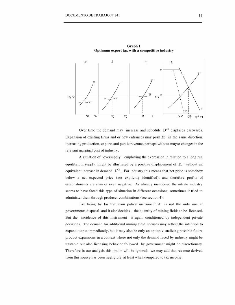
In graph 1, right side, industry’s marginal cost, Σc’, and marginal revenue, R’,

are obtained from nitrate demand faced by Chile, DCh. The export quantity identified

when equalizing both concepts illuminates the fiscal revenue maximizing mark-up, T*,

as the difference between marginal cost and the corresponding price for consumers. On

the other hand Σc’ represents the sum over individual firms (establishments) marginal

cost, c´. Net price, equal to monopoly profit maximizing price, P* minus T* is then the

guide to output determination, that is price faced at producer establishment level.

Heterogeneity in industry is illustrated in the graph by the presence of three

type of producers: α, β and γ. Under this tax scheme and meanwhile α and β are

registering positive profits, establishment γ is the marginal producer. These intra

marginal profits, not to be confused with monopoly revenue which here is captured

exclusively by government, may stand for quite a range of situations, non market

pricing of inputs comes here easily to mind; for example, nitrate content of minerals or

aspects related to establishments location, as distance from ports and access to water

supply (a critical factor in the desert).

Another way for expressing the same idea would have average cost equal to net

price for all establishments, case where all resources would be priced at the

corresponding shadow wage price. Finally the eventual difference among short and long

run average cost due to the existence of fixed factors in the former period will play an

important role, but its presentation is delayed until final discussion.


Graph 1Optimum export tax with a competitive industry

Over time the demand may increase and schedule DCh displaces eastwards.

Expansion of existing firms and or new entrances may push Σc’ in the same direction,

increasing production, exports and public revenue, perhaps without mayor changes in the

relevant marginal cost of industry.

A situation of “oversupply”, employing the expression in relation to a long run

equilibrium supply, might be illustrated by a positive displacement of Σc’ without an

equivalent increase in demand, DCh. For industry this means that net price is somehow

below a net expected price (not explicitly identified), and therefore profits of

establishments are slim or even negative. As already mentioned the nitrate industry

seems to have faced this type of situation in different occasions; sometimes it tried to

administer them through producer combinations (see section 4).

Tax being by far the main policy instrument it is not the only one at

governments disposal, and it also decides the quantity of mining fields to be licensed.

But the incidence of this instrument is again conditioned by independent private

decisions. The demand for additional mining field licenses may reflect the intention to

expand output immediately, but it may also be only an option visualizing possible future

product expansions in a context where not only the demand faced by industry might be

unstable but also licensing behavior followed by government might be discretionary.

Therefore in our analysis this option will be ignored; we may add that revenue derived

from this source has been negligible, at least when compared to tax income.


From 1880 onwards the specific tax measured in gold units, T (without supra

script, the effective tax) was applied, therefore the question to be evaluated period after

period collapses into the comparison of T* with T. Turning again to Graph 1, if the tax

T exceeds T*, or falls short of it , in both cases fiscal revenue stemming directly from

nitrates should not be at its theoretical maximum. For example, if T<T*, the difference

means that fiscal revenue would have been higher with a smaller export level, - the profit

maximizing QCh*- and a tax equal to T*. Since T is fixed a priori by law and is not a

consequence of a maximization process conditioned by the yearly outlook, the

possibility of a difference between actual and optimum tax is a very real issue.

The challenge facing Congress (public authority) when choosing the export tax

level was no minor task. It is our hypothesis that the objective function12 of these

authorities can be understood as maximization of public revenue stemming from nitrates,

but one needs to add that for political and economic reasons the yearly redefinition of the

tax should be prohibitive.13 The tax horizon is really not part of the discussion: for all

practical purposes once fixed it cannot be changed, unless of course something really

dramatic happens. In this scenario the experimental method of tax fixing, that is finding

maximum profits through a process of successive approximations was a non available

policy instrument.

Two aspects should be kept in mind. The first as already mentioned is that the

tax is fixed a priori by law and is not the consequence of a yearly maximization process

conditioned by the respective outlook. The second one centers on the particular

conditions posed by Graph 1 where a lineal demand curve implies a constantly changing

elasticity and therefore marginal revenue. Optimum mark-up T* is unique and could be

easily established provided the required information were available, the demand curve

itself. But this is not the case in our simulations and as will be seen in the next section

12 A discussion of tax approval in a public choice setting is here avoided. From a strictly rational point ofview there should not have been much opposition: the tax was supposed to be paid by the rest of the world, itwas also an opportunity to lower domestic taxes, the excise on tobacco being the main example. Of coursesome representatives related to existent producers and railroad interests, either Chilean or foreign, exercisedsome opposition.13 In a counterfactual scenario authorities would have enough commercial and analytical capacity and couldhave found the optimum export tax for each year. But in practice they were not given the discretionary powerfor doing it. Of course it is also possible that these optimizing capacities of the public bureaucracy wasrecognized as inexistent, be it for technical and informational reasons or be it because of eventual agencyproblem conflicts, and that precisely for this reason the tax was fixed by law and not changed. Implicit in thisdiscussion favoring a stable tax is the issue of the possible incidence of unexpected tax changes on industry’sinvestment. These institutional dimension of the nitrate export tax are not examined in the present paper.


our procedure is of a more speculative character, and only a set of plausible elasticities

are constructed. This procedure conditions the interpretation of our results (section 3.3).

3.2. Estimation and Data

(i) Optimum Tax

The traditional profit maximizing condition, marginal revenue equals marginal

cost,

P (1+(1/η)) = c’

defines optimum price , P*, as

P* = c’ [1/(1+(1/η))]

Therefore, the optimum tax (T*) is simply the difference between P* and cost,

and the tax efficiency indicator to be used is T/T*, effective over optimum export tax.

Two inputs are required for the determination of T*: cost and elasticity. The

former, given the above competitive equilibrium scenario, is simply understood being

equal to P-T, that is price minus tax, both effectively observed. The determination of the

second one is explained below.

(ii) Demand Elasticity

The demand elasticity faced by Chile is obtained thru an traditional excess

demand formulation:

ηch = (Qt/Qch)*ηwd – (Qr/Qch)*ξr

where

Qt. = World (total) production (consumption)

Qch = Chile’s exports (we ignore the insignificant difference between production and

exports)

Qr = competitor’s production


This demand elasticity faced by government , ηch, combines market

participation ratios (Table A1) with a set of a priori values for the world demand

elasticity for nitrates (ηwd) and for the supply elasticity of competitors(ξr).

Simulations are supposed to generate an elasticity for each particular year,

therefore and specially in the case of ξr they constitute short run or year specific values.

In the longer run, that is when taking into account the reaction to price changes over

more extended periods, ξr eventually may turn out being quite elastic, accounting for

expansions and innovations by actual and potential competitors, a possibility to be taken

into account when it comes to the evaluation of yearly results obtained.

The fourteen a priori selected elasticity combinations for generating ηch are the

following:

Table 3World Demand Elasticity for Nitrates and Competitors Supply Elasticity:

A priori estimates

ηwd ξr ηwd ξr-0,5 3 -0,2 1

-1 1 -0,2 0,7-0,7 1 0 1

-1 0 -1 3-0,5 1 -1 2-0,7 0,2 -1,5 1-0,5 0,5 -2 1

Due to its unreasonable marginal cost implication any elasticity equal to one or

less in absolute value, that is inelastic, is eliminated . The rest is synthesized into four

series, each registering an elasticity for every year:14

14 Direct econometric estimations of Chilean demand elasticity did not generate acceptable results. But areasonable estimate for World demand elasticity could be obtained from the 1880-World War I period. Theestimated equation is the following (all variables in logs):

Dependent Variable Constant London Price GDP (selectedcountries)

R2 (%)

World Production -18.55(-4.59)

-1.15(-3.14)

2.77(15.5)

92.7

Table 3 above was re-estimated with the same inputs for competitors supply elasticity and participation ratesbut now taking the econometric estimation for World demand elasticity, that is –1.15. In relation to theChilean elasticities estimates (1) and (4) above, and with the exception of elasticity (1) where this newprocedure generates significantly higher values, the three others show little difference with simulations in thefirst four columns of Table A.2. They are somewhat lower up to the first half of the period and definitively alittle after World War I (range from –20 per cent up to +15 per cent, depending on the elasticity).


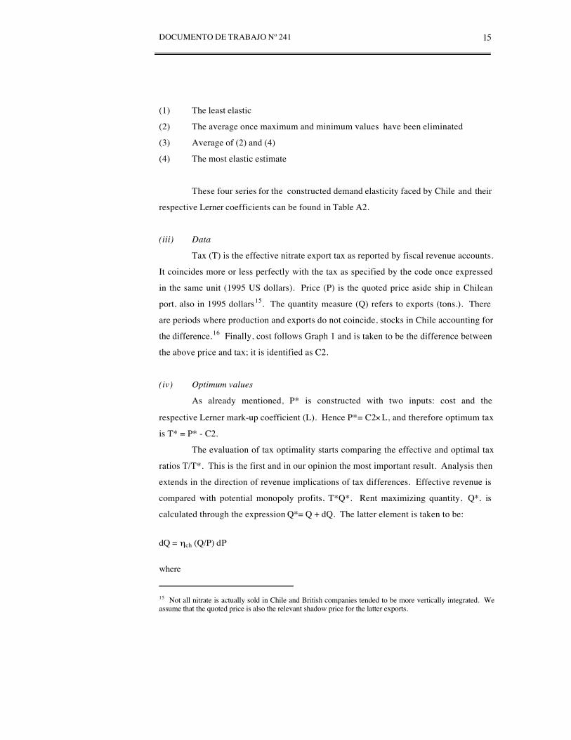
(1) The least elastic

(2) The average once maximum and minimum values have been eliminated

(3) Average of (2) and (4)

(4) The most elastic estimate

These four series for the constructed demand elasticity faced by Chile and their

respective Lerner coefficients can be found in Table A2.

(iii) Data

Tax (T) is the effective nitrate export tax as reported by fiscal revenue accounts.

It coincides more or less perfectly with the tax as specified by the code once expressed

in the same unit (1995 US dollars). Price (P) is the quoted price aside ship in Chilean

port, also in 1995 dollars15. The quantity measure (Q) refers to exports (tons.). There

are periods where production and exports do not coincide, stocks in Chile accounting for

the difference.16 Finally, cost follows Graph 1 and is taken to be the difference between

the above price and tax; it is identified as C2.

(iv) Optimum values

As already mentioned, P* is constructed with two inputs: cost and the

respective Lerner mark-up coefficient (L). Hence P*= C2×L, and therefore optimum tax

is T* = P* - C2.

The evaluation of tax optimality starts comparing the effective and optimal tax

ratios T/T*. This is the first and in our opinion the most important result. Analysis then

extends in the direction of revenue implications of tax differences. Effective revenue is

compared with potential monopoly profits, T*Q*. Rent maximizing quantity, Q*, is

calculated through the expression Q*= Q + dQ. The latter element is taken to be:

dQ = ηch (Q/P) dP

where

15 Not all nitrate is actually sold in Chile and British companies tended to be more vertically integrated. Weassume that the quoted price is also the relevant shadow price for the latter exports.


dP = (P* - P)

When P* turns out to be above P, then the optimum quantity Q* should be less

than Q, the actual export. Since Q and P are necessarily positive, the negative sign of

the demand elasticity determines the required negative dQ.

When comparing the effective and the optimum revenue it is necessary to keep

in mind that, as mentioned in 3.1, calculations are based on constructed elasticities. In

particular when calculating Q*, the elasticity implicit in both, Q and Q* is forced to be

the same, opening up the possibility of an effective revenue near to or even larger than

the theoretical optimum (once lack of precision of discrete calculations is

acknowledged). No exogenous test for the constructed elasticity is applied and therefore

a constant elasticity in the range Q-Q* cannot be ruled out a fortiori, neither confirmed.

In other words, a constant demand elasticity implies constant marginal revenue,

and when assuming scale independent unit costs as we do, it gives rise to a range of

profit maximizing export levels. Therefore the particular elasticity assumption opens up

the possibility for similarity, eventually identity, among effective and optimum public

revenue from nitrates, even if T* ≠ T.

3.3. Results

The ratio of real to optimal nitrate export tax for each of the above constructed

demand elasticity faced by Chile is shown in the initial four columns of Table A3. The

following set of four columns in the same Table depicts the ratios of real to optimum

exports, Q/Q*.

The ratio of T/T* for the least elastic value (1) is characterized by enormous

differences, implying that the real tax should have been ten, twenty or even more times

higher, implying an absurd corollary: Q*, the optimum export volume turns out negative

in most years. Our interpretation is that the assumed elasticity is too small and not

useful for evaluating the optimality issue.

16 Sales to consumers, mainly agriculture, and Chilean exports are not necessarily equal on a year by yearbasis. Data on stocks of Chilean nitrate in Europe is only available for a few more recent years. Due to thislimitation our calculations are based on exports and not strictly on consumption.


Calculations based on elasticity four, the most elastic are the only ones

generating positive Q/Q* ratios for the whole period. Elasticity two and also three

generate positive Q/Q* ratios, except for early years. The tax was established in 1880,

and assuming some rationality and reasonable information by the tax fixers, it is

precisely in those years where an acceptable fit should be expected. 17 Therefore at least

for those years only ratios based on elasticity four answers our main question; for later

years the T/T* ratios based on elasticity 2 and 3 cannot be eliminated from discussion.

The last four columns of Table A3 take the two measures together and compare

actual and optimum fiscal revenue. The first aspect to be noticed when centering

attention only on the most elastic case (4), underlines that even if deviations between

actual and optimum quantities are significant, real and optimum revenue tend to be

similar. When taking this figures without further consideration the optimum monopoly

quantity in practice turns out being a broad range of quantities and not a unique point.

In others words and referring again to Graph 1, marginal revenue and cost are more or

less equal for a range of quantities. But as discussed in the last section, the result needs

careful interpretation because of its implicit conditioning by basic methodological

procedures, in particular the constant elasticity assumption when calculating Q* (and

constant cost).

In Table A4 the first four columns show the same ratios of effective to optimum

revenue, but now imposing the additional condition that the coefficient stays within the

range: 0<coefficient<1,09 The lower limit simply eliminates all negative values,

because of their implicit negative optimum export quantity. The upper limit on the other

hand is more discretionary, leaving aside cases in which effective revenue is 10 per cent

and more higher than estimated under maximizing conditions. The argument behind this

restriction is empirical based on the notion that an excessive ratio of effective over

optimal revenue puts the simulated values under critical light. But, what is excessive?

Even if discretionary we postulate that an estimation error of less than 10 per cent is

tolerable. Of course a purist’s approach may want to reduce it to a still lower limit,

eliminating all cases above unity.

17 The tax was approved by parliament but in our understanding its level was heavily influenced by theproposition of the executive. Before that the issue was studied by a special committee.


The last set of four columns in Table A4 reproduces only indicators of the first

group surviving the test, therefore all T/T* ratios not complying with the above

condition disappear.


When accepting the revenue consequences as established by ratio TQ/T*Q* and

also the above criterion of positive coefficients below the ten per cent difference, then a

value of T/T* above unity literally implies that effective tax could have been reduced

without paying a revenue slice. But even if the conclusion is conditional to the

acceptance of this criteria, the important aspect to notice is the rising trend which

remains for the T/T* at least for the cases of elasticities 3 and 4. This upward trend in

later years will be interpreted as a policy opportunity for tax reduction without loss of

public revenue ( but more on this , later in section 6). Additionally, a lowering of the tax

within a reasonable range might also have helped industry’s competitive position.

4. PRIVATE PARTICIPATION IN MONOPOLY RENTS. DID IT EXIST?

In section 3 the assumed competitive environment translates into an industry

supply where cost is identified by the observed price minus real tax and the government

receives the monopoly rent. This scenario will now be modified so that additional

possibilities may be evaluated. On the one hand a broader participation scheme in the

above monopoly rent will be allowed for, and on the other the `possibility of a second

stage monopoly is introduced.

4.1. Private participation in the one stage monopoly context?

Nitrate historians inform about different privately induced cartel agreements

(“combinaciones”) each lasting for a short period of years. Agreements are said to have

been either ineffective in obtaining reductions of production or if registering some

success, did not work for long. Taken strictly these reports do not imply permanent

private participation in those monopoly rents, but the possibility is explored in what

follows.

The evaluation of this broader participation schemes in monopoly rents was

facilitated by cost data found when searching for nitrate facts, a data series stretching


from 1880 up to 1925.18 In this way price may be decomposed into: tax, cost and a

residual and once the latter is interpreted as profit a first step for a broader participation

scheme emerges.

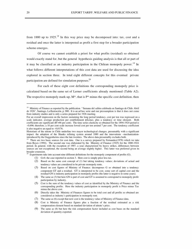
Of course we cannot establish a priori for what profits (residual) so obtained

would exactly stand for, but the general hypothesis guiding analysis is that all or part of

it may be classified as an industry participation in the Chilean monopoly power.19 In

what follows different interpretations of this cost data are used for discussing the idea

explored in section three. In total eight different concepts for this eventual private

participation are defined for simulation purposes.20

For each of these eight cost definitions the corresponding monopoly price is

calculated based on the same set of Lerner coefficients already mentioned (Table A2).

The respective monopoly mark-up, M*, that is P* minus the specific cost definition, then

18 Ministry of Finance as reported by the publication “Semana del salitre celebrada en Santiago de Chile Abrilde 1926”, Santiago, La Ilustración, p. 900. It is an ad hoc serie and our pressumption is that it does not comefrom industry studies and is only a series prepared for 1926 meeting.For an overall impression on the factors sustaining the long period tendency, cost per ton was regressed on ascale indicator, average production per establishment (oficina), plus a tendency or time element. Bothcoefficients are significant (R2=66 per cent). The time series elasticity so obtained for the 1894-1924 period is–0,696; therefore, a 10 per cent scale increase lowed cost per ton around 7 per cent. The tendency coefficientis also negative an equal to –0,0176.Historians of the nitrate in Chile underline two mayor technological changes, presumably with a significantimpact: the adoption of the Shanks refining system around 1880 and the innovations –mechanization-introduced by the Guggenheims since the late twenties. The above data presumably excludes both.19 There are two basic sources for cost data. One is a survey prepared by Fernandez(1978) which we takefrom Reyes (1994). The second one was elaborated by the Ministry of Finance (1925) for the 1880-1924period. In general, with the exception of 1907, a year characterized by heavy strikes, differences betweensources are not exceptional, the second being an average slightly higher. This latter was preferred given itsbroader extension.20 Experiments take into account nine different definitions for the monopoly component of profits (G).

(1) G=0, the case reported in section 3. Here cost is simply price less tax.(2) Based on the same cost concept of (1) but taking tendency values; deviations of actual and

tendency values are considered to be private monopoly rents.(3) Based on cost figures of Ministry of Finance; decomposes G so obtained into a tendency

component GT and a residual. GT is interpreted to be cost, some sort of capital cost and theresidual GN is industry participation in monopoly profits (the latter is negative in some years).

(4) The same as (3) but here GN is part of cost and GT is assumed to correspond to monopoly profitparticipation by industry.

(5) Cost is the sum of the tendency values of cost as identified by the Ministry of Finance and thecorresponding profits. Here the industry participation in monopoly profit is Price minus Taxminus the above cost.

(6) Directly takes the Ministry of Finances figures to be total cost and all profits so obtained areconsidered as industry’s participation in monopoly rent.

(7) The same as (6) except that now cost is the tendency value of Ministry of Finance data.(8) Cost is Ministry of Finance figures plus a fraction of the residual estimated as a risk

compensation element based on standard deviation of nitrate’s price.(9) The same as (8) but here the risk compensation factor included as cost bases on the standard

deviation of quantity exported.


distributes into tax and private monopoly profit participation (GP). Therefore M* = (TP

+ GP)*.

Notice that this scenario does not generate a measure for the revenue

maximizing tax as in section 3; it only determines the optimum mark-up M* but not its

distribution into tax and private profit. Additionally, government is also restricted by the

specifications of the tax law of the early 1880’s, having no capacity for yearly

negotiations, therefore TP = T and GP absorbs fluctuations in M* (in a few cases GP

turns out being negative).

It should also be noticed that the exercise simply assumes some sort of private

participation in monopoly rents and then explores its consequences, but it does not

provide an explicit justification for the existence of this participation.21

4.1.1. Results

As in section 3 and using the same set of elasticities the effective monopoly

returns are calculated; are visualizing them as the effective tax plus the corresponding

industry participation magnitude in relation to optimum monopoly mark-up, that is

(T+G)Q/(T+G)*Q*. Additionally we identify (T+G)/(T+G)*, that is the actual to

optimum mark-up, for those ratios within a range running from 0 up to 1.09.

Only from 1915 onwards and for all cost definitions is this ratio accepted by the

above test in the case of simulations based on the least elastic demand (η1), what brings

us to dismiss indicators developed under this elasticity assumption.

On the other hand for the most elastic demand (η4) assumption it is possible to

observe mark-up ratios since 1880, but more than half disappear after 1907. The

difficulty with the surviving indicators stretching over most of the fifty year period, is

that their usually high values, above unity suggest that already in the 1880’s and 1890’s

total mark-up tended to be excessive in a systematic fashion, a situation difficult to

believe for the early years.

Mark-up ratios computed with intermediate elasticity values (η2 and η3) and

similar to the most elastic case (η4), show half of the indicators disappearing between

21 There are different candidates for explaining private participation; cartel agreements already mentionedbeing one; maybe government licensing of new fields could be another one. The railroad Company is said tohave exercised market power (due to the government concession scheme) specially in the first decades. Butthis should not show up in the above GP since all of our cost definitions already account for this freight.


the years 1908 and 1912 and from then onwards. The rest, those covering a more

substantial part of the total period register more observations in the η3 case than in the

η2 case. Both elasticities generate indicators nearer to an interpretation where in the

initial years mark-up is somewhat below optimum, but turning definitively excessive in

the 1920; but some already point towards an excessive margin in the 1890’s.

It seems clear to us that this ratios might be criticized for proposing irrational

behavior by private participants: an excessive margin and considering the tax as given

would reflect an non optimizing adjustment. Abstaining from this limitation, these

results do not argue themselves in favor or against the hypothesis of a broader

participation scheme. Rather they show that if the analytical scenario allows for private

participation, then the general impression obtained in section 3 is still valid: may be too

little was charged in the early years, but it definitively became too large later on, a

consistent finding for all surviving indicators for the 1920’s.

4.2. Second Stage Monopoly?

Price distributes into cost, profit and tax in highly varying proportions; for

example, tax shares calculated over the FAS price go from a maximum of 47 per cent to

a minimum of 12 per cent (see Appendix, Table A1) following no precise time trend.

But since consumption localizes mainly in Europe and USA the above price, used in all

previous calculations, only represents the cost of one bundle of inputs of the product

finally consumed , the difference being sea freight, trade and financial services.22

Public debate with respect to nitrate policy considered this particular aspect to

be a weak feature in government control over nitrate business. The particular question

for our present purpose is the extent to which this margin, that is London-FAS price23,

22 Nitrate establishments localized in northern provinces were owned by proprietors of different nationalitiesincluding Chilean ones (proportions varied much through the period, in part only of a spurious reflection of theintroduction of corporate taxes in Great Britain). Loosely speaking we may say that British ownedestablishments exported directly, but the rest really were selling the product in Chile.23 Both London and FAS prices are yearly averages. At least in London’s case, it corresponds to a yearlyaverage, with clearly different maximum and minimum observations. We ignore how the averages werecomputed.


obeys exclusively to cost or if it also contains some element of market power.

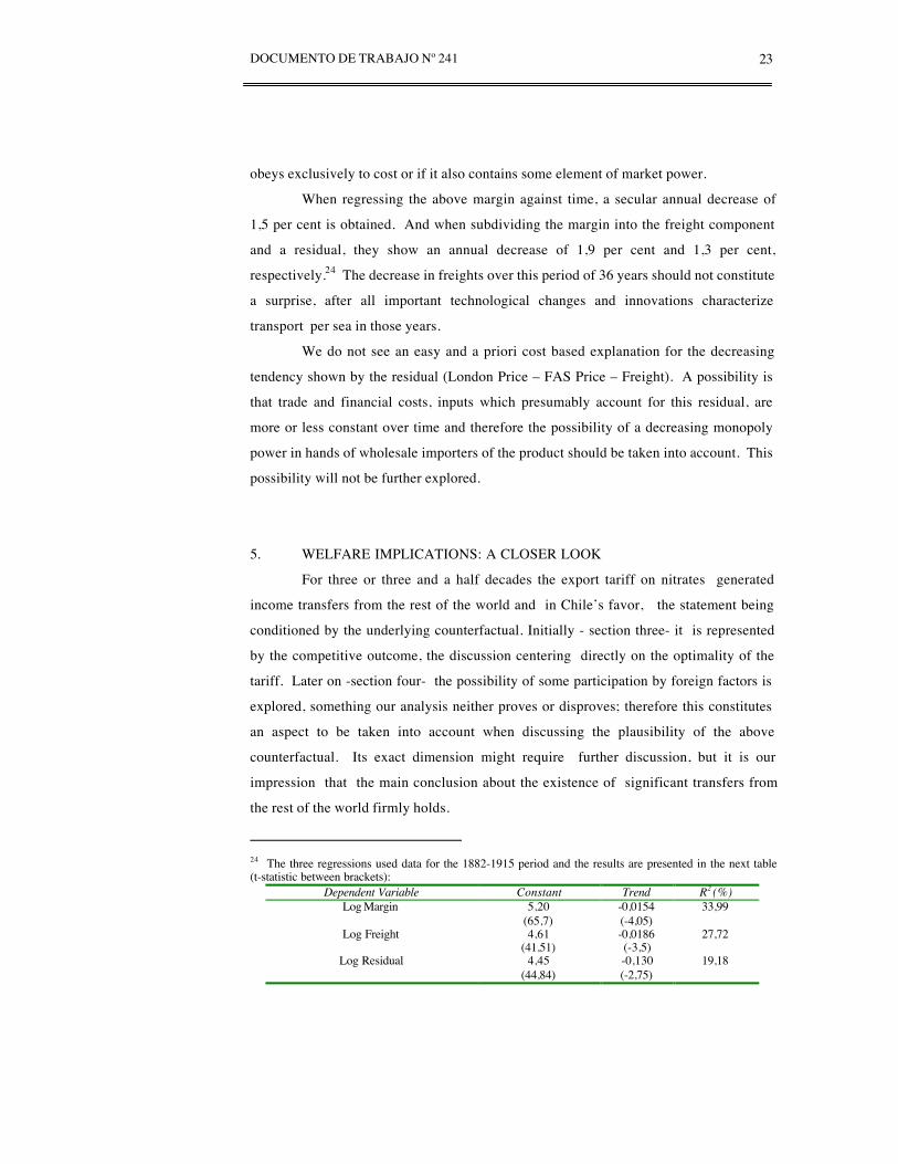
When regressing the above margin against time, a secular annual decrease of

1,5 per cent is obtained. And when subdividing the margin into the freight component

and a residual, they show an annual decrease of 1,9 per cent and 1,3 per cent,

respectively.24 The decrease in freights over this period of 36 years should not constitute

a surprise, after all important technological changes and innovations characterize

transport per sea in those years.

We do not see an easy and a priori cost based explanation for the decreasing

tendency shown by the residual (London Price – FAS Price – Freight). A possibility is

that trade and financial costs, inputs which presumably account for this residual, are

more or less constant over time and therefore the possibility of a decreasing monopoly

power in hands of wholesale importers of the product should be taken into account. This

possibility will not be further explored.

5. WELFARE IMPLICATIONS: A CLOSER LOOK

For three or three and a half decades the export tariff on nitrates generated

income transfers from the rest of the world and in Chile’s favor, the statement being

conditioned by the underlying counterfactual. Initially - section three- it is represented

by the competitive outcome, the discussion centering directly on the optimality of the

tariff. Later on -section four- the possibility of some participation by foreign factors is

explored, something our analysis neither proves or disproves; therefore this constitutes

an aspect to be taken into account when discussing the plausibility of the above

counterfactual. Its exact dimension might require further discussion, but it is our

impression that the main conclusion about the existence of significant transfers from

the rest of the world firmly holds.

24 The three regressions used data for the 1882-1915 period and the results are presented in the next table(t-statistic between brackets):

Dependent Variable Constant Trend R2 (%)Log Margin 5,20

(65,7)-0,0154(-4,05)

33,99

Log Freight 4,61(41,51)

-0,0186(-3,5)

27,72

Log Residual 4,45(44,84)

-0,130(-2,75)

19,18


Jumping directly from transfers to welfare implications smacks of partial or

incomplete analysis and for avoiding it at least two potential issues should be discussed.

Retaliation by trade partners is one aspect; the second assumes that welfare associates

with goods consumed and given no unique relation running from foreign transfers to the

level and composition of output, decisions pertaining public sectors expenditure may

play a central role. The present section discusses both briefly.

i) Retaliation by importers

Trade partner reactions to interventions in the free market for goods and

resources constitute a possible danger to any tariff measure, and retaliation may express

itself in many different ways: tariffs, quotas, an unsolicited visit of the fleet, etc.

The possibility of retaliation to nitrate’s export tax seems absent from Chilean

public policy discussions. But this is only an impression and not a conclusion flowing

from rigorous historical analysis, something the authors feel not prepared to realize;

recognizing this in what follows the above statement is taken only as a working

hypothesis.25 It is only in the late twenties and specially with the Great Depression that

regulatory reactions of trade partners start to inhibit nitrate exports, but and as our

discussion suggests in those years Chile already was nearer to a price taker than fixer

position and therefore its capacity for obtaining transfers thru trade taxes is quite

limited, probably inexistent

The overall transfer from trade partners provoked by the export tax includes, (i)

effective tax receipts by the Chilean government plus (ii) the respective Harberger

triangle,26 once free competitive world trade is taken as the pertinent counterfactual.

Total excise so defined when compared to a rough estimate of total agricultural GDP of

25 For example, a revision of the correspondence of the UK Foreign Office and its Chilean representatives, andalso internal letters of large British trade houses may possibly change this view.26 The standard expression for the excessive charge, for example Stiglitz (1988, Ch.18) when assuming elasticmarginal cost conditions, is given by 0.5*τ2*P*Q*η, where τ stands for the equivalent ad valorem taxcalculated over net supply price (P), Q is quantity, and η is demand elasticity. We estimated the magnitude ofthe excessive charge for the year 1900; P is equivalent to Chilean marginal cost (FAS price minus tax, T) andQ to Chilean exports divided by market participation, therefore a proxy for world volume. For price and taxwe take the corresponding averages for the 1895-1905 period. Our procedure assumes that all foreignproduction generates excessive charge from the point of view of world consumers. The total excise soobtained, that is excessive charge plus revenue so defined –chilean tax receipts plus the foreign productioneffect- gives a total of 477million 1995 US dollars. When comparing to a rough estimate of the main importingcountries agricultural sector GDP this total excise is equal to one fifth of I%.


main importers (our sample includes only UK, USA, Germany, Spain and France),

gives a cost equal to one fifth of one percent.27

There may also have been other issues explaining the apparent absence of

retaliation, about their relevance we can only speculate. One of them derives from the

heavy presence of foreign ownership in nitrate manufacture. Since any retaliation could

quite possibly have had a negative incidence on these interests, industry’s property

structure may have protected Chile’s monopoly power, at least in the short run.

Secondly international creditors were involved in industry itself, but also maintained

obligations issued by the Chilean government. Assuming that retaliation in response

to the export tax might have generated difficulties for debt servicing capacity, the inter

relations so obtained could have been a sort of stabilizing element in the scenario.

ii) Optimal export tariff and Chilean welfare.

Once nitrate fields came under Chilean jurisdiction and government starts

extracting those rents, public revenue expands rapidly; in this context one obvious

question refers to its translation into effective welfare. Judging the situation on a

simple normative scenario where citizens preferences are to be taken into account, and

where the demand behavior of the different goods consumed is assumed to be normal,

such an income shock would divide among state and citizens. With two composite

goods entering citizens utility function –let us say one private one public- the revenue

expansion distributes into both goods (Bradford and Oates 1971).

An empirical impression can be obtained when Chilean fiscal expenditure is

taken as representing the public good, and GDP minus fiscal expenditure as the private

one. Table 5 proportions income elasticities for these goods and for two periods,

before the nitrate episode and for three decades from 1880 onwards. According to these

results nitrate revenues open up new or formerly hidden dimensions of the Chilean

public choice process.

27 As explained in the previous footnote total excise represents a negligible fraction of production. What ismore surprising is the implicit cost of public funds; when taking the role of a world wide planer, each dollar ofChilean revenue so obtained costs the world 37 cents.But of course, Chilean government was not accountable for this cost; without retaliation it was irrelevant for itsconstituency.


Table 5Private and Public Good: Income Elasticities

(Pre and post 1880) 28

Private Good Public Good

1840-1880 1.04 0.78

1880-1910 0.85 2.24

The following Graph on the other hand , registers actual figures from 1870 up

to 1890 and from 1880 onwards incorporates projections based on first periods

elasticities29. Income expansion obtained from nitrates translates mostly into public

sectors expansion, resembling a distribution governed by the flypaper effect as it is

known in the literature referring to transfers from central to local governments (“money

sticks where it falls on”).30

0

50

100

150

200

250

1870

1871

1872

1873

1874

1875

1876

1877

1878

1879

1880

1881

1882

1883

1884

1885

1886

1887

1888

1889

1890

Public Good PbG PROJ

0

20

40

60

80

100

120

140

1870

1871

1872

1873

1874

1875

1876

1877

1878

1879

1880

1881

1882

1883

1884

1885

1886

1887

1888

1889

1890

Private Good PvG PROJ

The above exercise contrasts the empirical with an assumed or historical

income elasticity and therefore the observed difference neither proves or disproves the

validity of the respective assumption. Its main objective is to call attention onto an

28 Elasticities are obtained in a single variable relationship between the respective good and GDP, using firstdifferences. The data source is Braun and others (2000). Specially in the first period the private good ascomputed is a very important component of GDP, hence the estimate of public good elasticity.29 The above empirical finding is opposed to some historical literature claiming that governments lost thegolden opportunity for the country not using these resources directly for fostering development; the least to besaid is that fiscal expenditure expansions are far from negligible. But it might be that the criticism rests onexpenditure decisions within the budget not referring to the income distribution decision between public andprivate goods, a question we leave here.30 For a recent survey applied to local public finance, where the local distribution of central governmenttransfers are examined, see Hines and Thaler (1995)


unexplored issue, that is a discussion of the nitrate episode with reference to a broad

public choice scenario in both periods, one where options and restrictions are properly

identified in the choice setting. For example, the understanding of nitrate’s incidence on

the public budget and finally on welfare should benefit from its discussion on a

general scenario where public expenditure in specific items are allowed a more active

role. Defense or eventually infrastructure might after all be somehow linked to

territorial expansion, much more at least then an elasticity comparison permits; in other

words the underlying technology, that is the production function of nitrates

incorporation into Chilean jurisdiction is eventually a more complex issue, a restriction

not to be ignored. But extensions like this we cannot examine further.

6. FINAL REMARKS

For half a century nitrate exports provided Chile’s government with a

generous income stream; from 1880 and up to 1930, discounted at the 10% rate, the

stock value of the public revenue flow derived from this base is equivalent to 65.7% of

1880’s GDP.31 The evolution of this flow of export tax receipts is far from uniform,

being highly irregular from World War I onwards, and with the exception of a few years

much below pre-war levels.

a) Tax incidence

The policy instrument thru which the potential revenue flow materializes, the

specific export tax measured in gold units, stayed constant over the whole period in

spite of the dwindling Chilean market power. Our main objective has been the

evaluation of the optimality of this tariff design, that is the extent to which it coincided

with the monopoly profit maximizing mark-up thru time, and in this sense clear signals

of a fundamental change can be observed around World War I, sooner or later

depending on the specific simulation; in particular in the 1920’s the coefficient of the

effective export tariff in relation to optimum mark up is significantly higher then its pre

war level. Nevertheless the capacity of the export tax for raising state revenue is still

31 The discounted flow refers to export tariff receipts. Import tariffs charged on the corresponding imports arenot included.


important; for example, in the boom years 1927-29 public income stemming from nitrate

still added up to 77 per cent of the historical maximum reached in 1911-13.

As mentioned the high level reached in those years by the effective to

monopoly maximizing mark-up can be seen as a normative indicator favoring tax

change. But now it is time for discussing the consequence on public revenue of an

eventual tax reduction.

Referring to this question various aspects should be taken into consideration. To

begin with optimum tariff simulations are specifically determined for each year, but on

the other hand, the same elasticity is employed when calculating the ratio of effective to

optimum revenue, in particular for obtaining the revenue maximizing quantity, Q*. In

this sense the similarity between both revenues, specially in the case of simulations 3

and 4, is a consequence of this procedure but not necessarily does it constitute a

reasonable prediction of effective revenue in face of an tariff reduction. Constant

elasticity demand curves not being guaranteed a priori, such a prediction would require

an independent indicator for eventual elasticity changes. This we do not provide and

therefore our estimates for optimum revenue do not answer such a question, an aspect to

be taken into account in the following discussion.

In a long run perspective and to the extent that world price is still influenced by

the Chilean tax, 32 one concludes that a lower tax would have been followed by a smaller

price. As long as this is valid, in other words as long as the country keeps some market

power and additionally expansions of production by third parties are characterized by an

non zero supply elasticity, then Chile’s long run participation in total output will be

endogenous to its previous export tax level, a higher present tax implying a lower future

share. Taking these considerations together the tax change comes under a more

favorable light: when lowering its level in year t, its impact on fiscal receipts of the same

year cannot be predicted by our calculations but a shrinking revenue is quite possible.

On the other hand and for future periods such a change might generate a larger share in

total world output and eventually even more fiscal income. This simple reasoning does

not provide any clue to possible lags and timing, and the overall evaluation of an

32 A simple regression of FAS price with effective nitrate export tax for 1881 up to 1910 generates a positivecoefficient for the tax.


eventual tax change should have required additional information, one being the long run

supply elasticity for foreign production.

As already said our estimations suggest a rapidly falling monopoly power from

World War I onwards, but and given the inherent limitation in our methodology

specially with respect to the foreign supply elasticity, the possibility of little or non

market power left in 1920 cannot be ignored.33 This brings us to the third dimension of

such a tax change, that is the effective market situation in those years. A correct

identification is not provided and only a hypothetical scenario is briefly discussed.

Hereunder suppose that the 1920’s already offered a sort of competitive price facing

scenario to Chilean nitrates, what then is the incidence of the export tax?

Fixed, that is nitrate specific assets behind establishment’s production functions

make this tax possible in the short period. Nevertheless in a steady state equilibrium

rents to be derived from those assets take the form of necessary income for long run

survival. In such a context, therefore, the export tax effectively charged in the 1920’s

should have inhibited Chilean production and exports would disappear completely in the

long run.

Steady state is only an assumption for describing a case of extreme tax

incidence, the real 1920’s surely offered deviations from this hypothetical scenario, and

eventually exogenous technological innovation or changes in factor prices and of

intermediate goods changes may have been helpful to industry.

Industry spokesman emphasized the excessive character of the tax, specially in

the 1920’s; in itself and as Adam Smith taught us, such expressions not necessarily

constitute unbiased opinion. But there is more and early reflections of a government

observer of the nitrate market, already in the first decade of 1900 confirm the presence

of stiffer foreign competition (Bertrand as quoted by Reyes 1994, pp.15-21). In the

second half of the 1920’s it is government itself who seems to recognize a problem

33 The econometric estimation of World demand elasticity (see footnote 15) already points to ward somewhathigher elasticity estimates than those underlying our calculations for the 1920’s.


when starting to return a fraction of revenue to industry.34 It also began to prepare a new

tax code and finally in 1930 the specific tax was repealed in favor of a tax on capital;

also a mayor reorganization imposed a centralized sales agency.

The hypothetical tax cut in year t, say in the 1920’s, would probably have

meant more or less similar production but less fiscal income in the same year; its long

run incidence on both variables remaining an open question. Such reasoning must

surely have been part of government reflections when it came to tax innovation.

Henceforth policy change must have been taken as a rather risky adventure, where quite

visible and negative immediate consequences could not have been turned around by

eventually positive long run effects, and this before introducing any consideration with

respect to governments rather reduced time horizons.

In the 1920’s, may be somewhat earlier, the different governments seem to have

found themselves in an ever increasing dilemma: (i) lower the export tax and face quite

possibly a simultaneous revenue decrease, but thru it also obtain an increment of the

probability of larger- compared to business as usual- future incomes from this source;

(ii) on the other hand, stick to the existing tax and at least obtain the “sure” thing now (a

way of saying since exports in that decade were highly variable). “Larger” future

income to be derived from a tax cut is expected and its presently perceived magnitude,

once taking into account the declining evolution of market participation experienced by

the country, could have been rather slim. Adding to this the agency problem which is

said to characterize governments in general when it comes to discount future income , it

is not surprising that the tax was maintained.

(b) The Great Depression: a defining moment for nitrate exports?

The incidence of the Great Depression of the 1930 is put under a new light by

our findings. By many accounts, see for example Cepal (1949), the depression is really a

34 Devolution by the “Caja de Fomento Salitrero” accounted for the following percentages of revenuesstemming from nitrates export tax (our data on revenues reported in this paper are therefore gross revenues):1927, 2 percent; 1928, 21 per cent; 1929, 26 per cent. Source: Rep. de Chile Ministerio de Hacienda, Of.Presupuesto, Folleto No. 27 Noviembre 1930, “ Compañia de Salitre de Chile”, p.8. Devolution based on law4.144, July 27th 1927, whose aim was to save the specific export tax established in 1880, probably under theassumption that the crisis industry was living was not permanent. Devolution itself had more of year by yeardiscretionary character and is therefore more similar to sudden unexpected capital gains than to industryincome to be included in project evaluation. The above reflection is included in the introduction to the lawproject creating the “Compañia Salitrera Nacional de Chile” in 1930, when also the specific export tax isrepealed and a centralized sales agency is created.


defining moment in Chile’s development, limiting its access to world markets and

pushing the country towards inward-looking policies. The depression is seen and

correctly we think, as a worldwide and completely exogenous phenomena imposing

itself on this small and export oriented country. But and this is the point we want to

emphasize the statement should not be turned around and simply understood as the

unique cause behind export contraction. The fall in exports we argue was additionally

conditioned by the domestic nitrate policy applied earlier. Our findings not only

underline the convenience of a broader scenario for the discussion of the depression,

they also suggests a qualitative answer: domestic public decisions or better absence of

decisions were quite relevant in nitrate’s collapse.35 The outbreak of the depression

probably helped in fixing the exact time point of the phenomena, but its more or less

definitive character has much deeper roots.

(c) Reflections on tax stability

For about three decades from 1880 onwards did the application of the export tax

generate quite satisfactory results, capturing rents and providing fiscal revenue. If the

tax was the best suited policy instrument available for exploiting the opportunity offered

by world demand and control of supply conditions is debatable. One may think of

alternatives offering more capacity of adaptation to changing market conditions, but tax

asessment and enforcement costs in general should not be forgotten when developing

such an exercise. Anyway even if the conclusion of such a search would bring us to

consider the nitrate tax as the best available instrument, it seems quite evident that this

inference should no longer be valid after World War I.

Remember now that the tax was established in gold pesos, and that once

metal’s price began to change the effective tax followed it closely. Comparing the

effective tax charged with a counterfactual one fixed in real dollars at the initial 1880

level, we find the first departing markedly from the second, as it can be seen in the

Graph A8. Until World War I, even if non negligible fluctuations are present, the tax

stays above the 75 per cent level (of 1880). A sharp decline follows and only in the

second half of 1920’s it climbs back to 55 per cent of its initial level.

35 One interesting future exercise would compare public policy towards nitrates and towards copper in the1920’s, the latter an export good rapidly recovering after 1930 and at least initially taxed by a quite differentand more flexible code. But this is a subject for another study


In other words, once monopoly power shows clear signs of rapid declination,

the tax adjusts accordingly. This can be seen as a lucky circumstance for tax survival,

but also as an additional variable to be taken into account when trying to understand why

government should have hesitated with tax changes. In this sense the upward trend of

the effective tax in the 20’s might have been an additional factor stimulating redesign

of the tax code.

Was there an alternative tax available? Strictly speaking this question may be

impossible to answer here, but a look at the tax treatment received by copper, the

sharply rising export activity of the 1920’s may throw some light on it. Reynolds (1965)

states “it is clear that taxation before 1925 was well below 5 per cent of the value of

sales” (p.226). Income tax in large scale copper production was not collected until 1922.

In 1925 and due to advice of the Kemmerer Mission, a 6 per cent levy on profits was

added.36

But again the overall impression to be obtained from copper’s tax experience is

that government cannot have found in it a very solid argument for tax change in nitrates.

As so many times in Chilean development policy, change required the presence of a

really sharp depression, but it came too late.

36 It is understood that Social Security taxes and regulations, heavily enforced in the copper sector, producedsome temporal increase in the wage bill of large copper mining (op. cit., p.228). The latter could be consideredas a short run tax-expenditure program with redistributive effects favoring labor in the sector.


REFERENCES

Ballard, Charles; John Shoven and John Walley (1985): “General EquilibriumComputations of the Marginal Welfare Cost of Taxes in the US”, American EconomicReview, Vol.75, No.1, pp.128-138

Bertrand, Alejandro (1910): La crisis salitrera (1910); estudio de sus causas y caracteresy de las condiciones favorables que caracterizan a la industria y comercio del salitre paraevolucionar en el sentido de su concentración económica. Paris, Luis Hechaud

Bertrand, Alejandro (1915): Estudio sobre la Industria y Comercio de SubstanciasAzoadas, considerando especialmente en cuanto se relaciona con la Industria y elComercio del Salitre de Chile, presentado al Ministerio de Hacienda de la Republica deChile. Julio 1915. Santiago, Soc. Imp. Lit. Barcelona

Bickerdike (1906) in Scitowsky (1987)

Bielschowsky, R. (1998): “Evolución de las ideas de la CEPAL”, Revista de la CEPAL,Special Issue

Braun, J.; M. Braun; I. Briones; J. Díaz; R. Lüders and G. Wagner (2000): EconomíaChilena 1810 – 1995. Estadísticas Históricas, Documento de Trabajo del Instituto deEconomía de la Pontificia Universidad Católica de Chile, No. 187

Bradford, D. and W. Oates (1971): “The analysis of revenue sharing in a new approachto collective fiscal decisions”, Quarterly Journal of Economics, Vol.85, No.3, pp.416-39

Brown, J. R. (1963): “Nitrate Crises, Combinations and the Chilean Government in theNitrate Age”, Hispanci American Historical Review, Vol.43

Cariola, Carmen and Osvaldo Sunkel (1982): La historia economica de Chile entre 1830y 1930: dos ensayos y una bibliografia. Madrid, Ediciones Cultura Hispanica ICI

Caves, Richard (1989): “International differences in Industrial Organization”, Chapter21 of Schamalensee and Willig (1989)

Cepal (1949): Economic Survey of Latin America. N.York, CEPAL

Corden, W. M. (1974): Trade Policy and Economic Welfare. Oxford, Oxford UniversityPress, Ch. 4

Fernandez, Manuel (1978): The development of the Chilean Economy and its BritishConnections, 1895-1914. PhD Thesis, University of Glasgow

Goode, Richard; George E. Lent and P.D. Ohja (1966) "Role of Export Taxes inDeveloping Countries", IMF Staff Papers, 13 November, 453-503


Hines, J. and R. Thaler (1995): “The flypaper effect”, Journal of Economic PerspectivesVol.9, No.4 (Fall), pp.217-226

Jofré, J.; Lüders, R. y G. Wagner (2000): "Economía Chilena 1810 - 1995. CuentasFiscales", Documento de Trabajo IEUC (Santiago), No. 188

Lewis Jr., Stephen R. (1963): "Government Revenue From Foreign Trade: anInternational Comparison" 1963. The Manchester School.

Lüders R. and G. Wagner (1998), "Two Centuries of Aggregate Fiscal Behavior inChile, A Small and at Times, Open Economy", draft, Institute of Economics, PontificalCatholic University, Santiago.

Lüders R. and Gert Wagner (1999): “The Great Depression and the Gold Standard:repercussion in a small and sometimes open economy. Chilean monetary experience”(mimeo)

Lüders, Rolf (1998): "The comparative economic performance of Chile: 1810-1995",Estudios de Economía (Santiago) Vol.25, No.2, pp.217-249

Ministry of Finance (1925): Antecedentes sobre la Industria salitrera 1925. Santiago,Soc. Imp. y Lit. Universo (Ministerio de Hacienda, Sección Salitre)

Ministry of Finance (1934): La Industria del Salitre de Chile. Santiago, La Nación

O’Brien, Thomas (1989): “’Rich beyond the dreams of avarice’: the Guggenheims inChile”, Business History Review, No.63 (Spring)

Peltzman, Sam (1977): “The gain and losses from industrial concentration”, Journal ofLaw and Economics (October)

Pomery, John (1987): The New Palgrave : A Dictionary of Economics, pp.732 ss.

Reyes, Enrique (1994): Salitre de Chile, Apertura, Inversión y Mercado Mundial, 1880-1925. Santiago, Universidad Católica Blas Cañas

Sapelli, Claudio (2001): “Concentración y Grupos Económicos en Chile”, Serie InformeEconómico Libertad y Desarrollo (Santiago), No. 121 (June)

Schmalensee, Richard (1989): “Inter Industry Studies of Structure and Performance”,Chapter 16 of Schamalensee and Willig (1989)

Schamalensee, R. and Willig, Robert (1989): Hanbook of Industrial Organization. NorthHolland

Scitowsky, Tibor (1987): The New Palgrave : A Dictionary of Economics, pp.586 ss.

Semana del Salitre (1926): Semana del Salitre celebrada en Santiago de Chile, Abril1926. Santiago, Imp. Lit. La Ilustración


Stiglitz, Joseph (1988): The economics of the public sector. W.W: Norton

Sutton, John(1997): “Gibrat’s Legacy”, Journal of Economic Literature, Vol.35, No.1(March)

Wallis, John Joseph (2000): “American Government Finance in the Long Run: 1790-1990”, Journal of Economic Perspectives Vol.14, No.1 (Winter), pp.61-82


APPENDIX

Table A1Chilean Nitrates 1880-1930: Basic Data (US$ 1995 per ton and shares)

FAS Price LondonPrice

Tax Cost Freight World AzoeProduction:Chile (%)

World AzoeProduction:Others (%)

1880 547,35 775,93 172,14 146,17 101,98 87,86 12,141881 446,37 697,06 127,80 247,13 129,11 89,18 10,821882 405,85 601,07 125,86 294,42 99,23 89,41 10,591883 371,67 554,08 134,73 287,77 101,57 88,62 11,381884 388,45 518,48 153,38 230,78 79,63 85,45 14,551885 460,97 604,37 159,95 184,91 86,96 78,30 21,701886 414,88 591,06 125,44 215,17 76,89 75,50 24,501887 363,07 563,00 136,22 213,40 82,43 79,89 20,111888 389,61 575,85 153,43 182,33 87,14 78,30 21,701889 392,73 570,37 161,98 200,91 93,07 77,90 22,101890 338,76 497,14 158,40 212,01 109,74 76,66 23,341891 374,63 536,62 133,28 214,58 106,56 72,66 27,341892 432,50 579,32 173,54 198,24 67,45 68,90 31,101893 423,94 610,41 166,64 163,88 80,73 71,03 28,971894 477,76 679,73 188,25 191,07 94,15 72,31 27,691895 423,50 582,98 179,89 256,51 86,23 73,33 26,671896 459,59 589,82 198,21 196,50 75,20 70,04 29,961897 427,25 572,31 173,70 240,12 77,56 67,49 32,511898 367,14 534,87 161,44 201,39 99,53 71,38 28,621899 357,47 523,94 169,51 196,52 90,49 71,16 28,841900 356,00 516,65 160,65 219,28 101,98 70,50 29,501901 433,57 557,70 166,45 196,35 74,90 67,53 32,471902 421,26 544,83 146,23 208,36 52,30 68,62 31,381903 417,35 548,59 149,25 257,59 44,68 70,38 29,621904 462,06 590,20 149,90 218,46 49,30 68,24 31,761905 482,86 616,26 151,29 233,24 57,11 67,68 32,321906 522,84 623,68 145,93 282,86 45,69 65,42 34,581907 506,24 585,05 135,72 330,48 37,17 62,60 37,401908 458,14 560,33 141,15 173,92 40,20 61,04 38,961909 385,67 497,70 131,14 176,86 45,73 59,61 40,391910 372,95 457,27 127,97 157,19 44,31 60,31 39,691911 431,68 524,26 137,79 172,34 49,78 57,88 42,121912 440,73 549,34 128,89 159,93 65,88 55,54 44,461913 428,87 543,98 123,91 187,23 64,22 54,32 45,681914 390,98 526,17 133,98 161,60 49,56 51,58 48,421915 379,94 616,31 127,15 170,90 166,52 33,73 66,271916 342,60 704,51 103,33 153,04 250,56 41,31 58,691917 407,96 321,80 83,20 136,31 224,01 38,38 61,621918 353,41 288,56 43,65 85,97 218,04 34,86 65,141919 285,65 219,79 55,57 123,97 164,76 30,58 69,421920 405,26 252,07 55,70 100,90 43,50 31,51 68,491921 423,77 478,72 76,24 130,96 43,31 32,31 67,691922 361,99 417,19 73,45 161,49 43,12 24,04 75,961923 353,47 655,70 81,46 154,96 42,93 32,20 67,801924 362,03 501,54 81,19 158,71 42,74 35,56 64,441925 332,17 347,38 86,05 129,77 42,55 33,93 66,071926 339,57 345,62 93,23 122,59 42,36 25,67 74,331927 310,74 337,91 102,24 113,57 42,17 19,52 80,481928 303,19 298,84 93,18 122,64 41,98 27,51 72,491929 286,13 298,04 95,04 120,78 41,80 24,17 75,831930 265,89 349,45 98,55 117,26 41,61 18,37 81,63

Estimates in cursive


Table A2Demand Elasticities and Lerner Coefficients Simulation, 1880-1930

Elasticity 1 Elasticity 2 Elasticity 3 Elasticity 4 LernerCoefficient 1

LernerCoefficient 2

LernerCoefficient 3

LernerCoefficient 4

1880 -1,14 -1,52 -1,97 -2,41 8,23 2,91 2,03 1,711881 -1,12 -1,47 -1,92 -2,36 9,24 3,11 2,09 1,731882 -1,12 -1,47 -1,91 -2,36 9,45 3,15 2,10 1,741883 -1,13 -1,49 -1,94 -2,39 8,79 3,02 2,06 1,721884 -1,10 -1,53 -2,02 -2,51 11,41 2,90 1,98 1,661885 -1,17 -1,74 -2,29 -2,83 6,85 2,35 1,78 1,551886 -1,25 -1,87 -2,42 -2,97 4,98 2,16 1,70 1,511887 -1,13 -1,67 -2,21 -2,76 8,82 2,49 1,82 1,571888 -1,17 -1,74 -2,29 -2,83 6,85 2,35 1,78 1,551889 -1,18 -1,76 -2,30 -2,85 6,49 2,32 1,77 1,541890 -1,22 -1,81 -2,36 -2,91 5,59 2,23 1,73 1,521891 -1,04 -1,80 -2,47 -3,13 26,92 2,25 1,68 1,471892 -1,11 -1,98 -2,67 -3,35 10,42 2,02 1,60 1,421893 -1,07 -1,88 -2,55 -3,22 15,93 2,14 1,64 1,451894 -1,04 -1,82 -2,48 -3,15 23,41 2,22 1,67 1,471895 -1,03 -1,77 -2,43 -3,09 37,62 2,29 1,70 1,481896 -1,09 -1,93 -2,61 -3,28 12,76 2,08 1,62 1,441897 -1,13 -2,06 -2,75 -3,45 8,49 1,95 1,57 1,411898 -1,06 -1,86 -2,53 -3,20 17,44 2,16 1,65 1,451899 -1,06 -1,87 -2,54 -3,22 16,43 2,15 1,65 1,451900 -1,08 -1,90 -2,58 -3,26 14,06 2,11 1,63 1,441901 -1,13 -2,05 -2,75 -3,44 8,54 1,95 1,57 1,411902 -1,11 -2,00 -2,68 -3,37 9,97 2,00 1,59 1,421903 -1,08 -1,91 -2,59 -3,26 13,70 2,10 1,63 1,441904 -1,12 -2,02 -2,71 -3,40 9,41 1,98 1,59 1,421905 -1,13 -2,05 -2,74 -3,43 8,70 1,96 1,57 1,411906 -1,03 -2,06 -2,82 -3,59 35,87 1,94 1,55 1,391907 -1,10 -2,21 -3,00 -3,79 11,26 1,83 1,50 1,361908 -1,14 -2,30 -3,11 -3,91 8,23 1,77 1,47 1,341909 -1,01 -2,27 -3,15 -4,03 76,54 1,79 1,46 1,331910 -1,16 -2,35 -3,16 -3,97 7,33 1,74 1,46 1,341911 -1,07 -2,38 -3,28 -4,18 14,64 1,73 1,44 1,311912 -1,16 -2,53 -3,47 -4,40 7,22 1,65 1,41 1,291913 -1,21 -2,61 -3,57 -4,52 5,78 1,62 1,39 1,281914 -1,04 -2,68 -3,75 -4,82 23,28 1,59 1,36 1,261915 -1,96 -4,45 -6,66 -8,86 2,04 1,29 1,18 1,131916 -1,42 -3,44 -5,06 -6,68 3,38 1,41 1,25 1,181917 -1,61 -3,79 -5,60 -7,42 2,65 1,36 1,22 1,161918 -1,87 -4,27 -6,37 -8,47 2,15 1,31 1,19 1,131919 -2,24 -5,02 -7,55 -10,08 1,80 1,25 1,15 1,111920 -2,16 -4,84 -7,27 -9,69 1,86 1,26 1,16 1,121921 -2,09 -4,69 -7,04 -9,38 1,92 1,27 1,17 1,121922 -3,04 -6,67 -10,16 -13,64 1,49 1,18 1,11 1,081923 -2,09 -4,71 -7,07 -9,42 1,91 1,27 1,16 1,121924 -1,81 -4,17 -6,21 -8,25 2,23 1,32 1,19 1,141925 -1,95 -4,42 -6,60 -8,79 2,06 1,29 1,18 1,131926 -2,81 -6,18 -9,38 -12,58 1,55 1,19 1,12 1,091927 -3,91 -8,46 -12,98 -17,49 1,34 1,13 1,08 1,061928 -2,57 -5,70 -8,62 -11,54 1,64 1,21 1,13 1,091929 -3,02 -6,63 -10,09 -13,55 1,49 1,18 1,11 1,081930 -4,20 -9,06 -13,92 -18,78 1,31 1,12 1,08 1,06


Table A3Tax Exports and Revenue: ratios of real to optimal, 1880-1930

Elast 1 Elast 2 Elast 3 Elast 4 Elast 1 Elast 2 Elast 3 Elast 4 Elast 1 Elast 2 Elast 3 Elast 4T/T* T/T* T/T* T/T* Q/Q* Q/Q* Q/Q* Q/Q* TQ/T*Q

*TQ/T*Q

*TQ/T*Q

*TQ/T*Q

*1880 0,06 0,24 0,44 0,65 -0,23 -1,93 19,85 1,70 -0,01 -0,46 8,82 1,101881 0,05 0,19 0,37 0,55 -0,19 -1,25 -6,28 2,27 -0,01 -0,24 -2,31 1,241882 0,05 0,21 0,41 0,61 -0,19 -1,39 -18,35 1,88 -0,01 -0,29 -7,51 1,151883 0,07 0,28 0,53 0,79 -0,24 -2,59 4,06 1,30 -0,02 -0,73 2,17 1,031884 0,06 0,34 0,66 0,99 -0,18 -6,51 2,00 1,01 -0,01 -2,23 1,33 1,001885 0,09 0,39 0,68 0,97 -0,33 15,00 1,84 1,03 -0,03 5,89 1,26 1,001886 0,11 0,37 0,62 0,86 -0,48 16,70 2,29 1,18 -0,05 6,26 1,41 1,011887 0,08 0,40 0,73 1,05 -0,24 14,02 1,63 0,95 -0,02 5,65 1,19 1,001888 0,11 0,48 0,83 1,19 -0,37 3,87 1,28 0,85 -0,04 1,86 1,07 1,011889 0,13 0,53 0,92 1,30 -0,43 2,78 1,12 0,79 -0,06 1,47 1,03 1,021890 0,19 0,71 1,20 1,68 -0,71 1,52 0,82 0,64 -0,14 1,08 0,98 1,081891 0,02 0,44 0,81 1,18 -0,06 5,13 1,36 0,86 0,00 2,28 1,10 1,011892 0,07 0,66 1,12 1,58 -0,21 1,70 0,88 0,67 -0,01 1,12 0,98 1,061893 0,04 0,57 1,00 1,44 -0,12 2,27 0,99 0,72 -0,01 1,29 1,00 1,041894 0,03 0,53 0,96 1,40 -0,08 2,70 1,05 0,74 0,00 1,44 1,01 1,031895 0,02 0,57 1,06 1,54 -0,05 2,31 0,93 0,68 0,00 1,32 0,99 1,061896 0,06 0,70 1,22 1,73 -0,17 1,54 0,80 0,63 -0,01 1,08 0,97 1,081897 0,09 0,72 1,20 1,68 -0,28 1,47 0,81 0,64 -0,03 1,06 0,97 1,071898 0,05 0,68 1,20 1,73 -0,12 1,64 0,81 0,63 -0,01 1,11 0,97 1,081899 0,06 0,79 1,39 2,00 -0,14 1,32 0,70 0,57 -0,01 1,04 0,97 1,131900 0,06 0,74 1,30 1,85 -0,16 1,42 0,75 0,60 -0,01 1,06 0,97 1,111901 0,08 0,66 1,09 1,52 -0,26 1,70 0,90 0,69 -0,02 1,12 0,98 1,051902 0,06 0,53 0,90 1,26 -0,20 2,59 1,16 0,80 -0,01 1,37 1,04 1,021903 0,04 0,51 0,88 1,26 -0,13 2,99 1,18 0,81 -0,01 1,51 1,04 1,021904 0,06 0,49 0,82 1,15 -0,20 3,18 1,32 0,87 -0,01 1,55 1,08 1,011905 0,06 0,48 0,79 1,11 -0,22 3,35 1,39 0,90 -0,01 1,60 1,10 1,001906 0,01 0,41 0,71 1,00 -0,04 5,79 1,72 1,00 0,00 2,37 1,21 1,001907 0,04 0,44 0,73 1,02 -0,14 3,89 1,59 0,98 -0,01 1,73 1,16 1,001908 0,06 0,58 0,94 1,30 -0,23 2,05 1,08 0,78 -0,01 1,19 1,02 1,021909 0,01 0,65 1,11 1,56 -0,02 1,69 0,88 0,67 0,00 1,10 0,98 1,051910 0,08 0,70 1,13 1,55 -0,29 1,51 0,87 0,67 -0,02 1,06 0,98 1,051911 0,03 0,64 1,07 1,49 -0,12 1,72 0,92 0,69 0,00 1,11 0,98 1,041912 0,07 0,63 1,02 1,41 -0,27 1,76 0,98 0,73 -0,02 1,11 1,00 1,031913 0,08 0,66 1,04 1,43 -0,36 1,66 0,95 0,72 -0,03 1,09 0,99 1,031914 0,02 0,88 1,43 1,99 -0,07 1,15 0,67 0,55 0,00 1,01 0,96 1,091915 0,49 1,74 2,84 3,95 3,30 0,61 0,34 0,31 1,60 1,06 0,97 1,231916 0,18 1,06 1,75 2,45 -1,07 0,95 0,54 0,46 -0,20 1,00 0,94 1,121917 0,16 0,71 1,18 1,65 -1,28 1,45 0,81 0,63 -0,20 1,03 0,96 1,031918 0,12 0,46 0,76 1,05 -1,53 2,61 1,50 0,95 -0,19 1,20 1,14 1,001919 0,30 0,97 1,58 2,19 -59,65 1,03 0,58 0,48 -17,91 1,00 0,92 1,061920 0,18 0,61 1,00 1,39 -3,20 1,73 1,00 0,73 -0,59 1,06 1,00 1,011921 0,24 0,81 1,32 1,84 -4,99 1,25 0,71 0,57 -1,19 1,01 0,94 1,041922 0,52 1,44 2,33 3,22 2,32 0,71 0,39 0,34 1,21 1,02 0,90 1,111923 0,33 1,11 1,82 2,52 95,89 0,90 0,51 0,43 31,44 1,00 0,92 1,091924 0,23 0,92 1,51 2,10 -3,09 1,09 0,62 0,51 -0,72 1,00 0,93 1,071925 0,33 1,20 1,96 2,72 -52,84 0,84 0,47 0,41 -17,50 1,01 0,93 1,121926 0,68 1,96 3,17 4,38 1,55 0,55 0,30 0,27 1,06 1,07 0,94 1,201927 1,43 3,66 5,87 8,09 0,72 0,33 0,17 0,17 1,03 1,21 1,02 1,341928 0,70 2,08 3,38 4,68 1,52 0,52 0,29 0,26 1,06 1,09 0,97 1,231929 1,01 2,80 4,52 6,24 0,99 0,41 0,22 0,21 1,00 1,16 1,00 1,311930 1,88 4,75 7,61 10,47 0,58 0,27 0,14 0,14 1,09 1,30 1,08 1,44


Table A4Tax Exports and Revenue: ratios of real to optimal, 1880-1930

Only if 0< TQ/T*Q* <1,09

Elast 1 Elast 2 Elast 3 Elast 4 Elast 1 Elast 2 Elast 3 Elast 4TQ/T*Q* TQ/T*Q* TQ/T*Q* TQ/T*Q* T/T* T/T* T/T* T/T*

1880188118821883 1,03 0,791884 1,00 0,991885 1,00 0,971886 1,01 0,861887 1,00 1,051888 1,07 1,01 0,83 1,191889 1,03 1,02 0,92 1,301890 1,08 0,98 1,08 0,71 1,20 1,681891 1,01 1,181892 0,98 1,06 1,12 1,581893 1,00 1,04 1,00 1,441894 1,01 1,03 0,96 1,401895 0,99 1,06 1,06 1,541896 1,08 0,97 1,08 0,70 1,22 1,731897 1,06 0,97 1,07 0,72 1,20 1,681898 0,97 1,08 1,20 1,731899 1,04 0,97 0,79 1,391900 1,06 0,97 0,74 1,301901 0,98 1,05 1,09 1,521902 1,04 1,02 0,90 1,261903 1,04 1,02 0,88 1,261904 1,08 1,01 0,82 1,151905 1,00 1,111906 1,00 1,001907 1,00 1,021908 1,02 1,02 0,94 1,301909 0,98 1,05 1,11 1,561910 1,06 0,98 1,05 0,70 1,13 1,551911 0,98 1,04 1,07 1,491912 1,00 1,03 1,02 1,411913 1,09 0,99 1,03 0,66 1,04 1,431914 1,01 0,96 0,88 1,431915 1,06 0,97 1,74 2,841916 1,00 0,94 1,06 1,751917 1,03 0,96 1,03 0,71 1,18 1,651918 1,00 1,051919 1,00 0,92 1,06 0,97 1,58 2,191920 1,06 1,00 1,01 0,61 1,00 1,391921 1,01 0,94 1,04 0,81 1,32 1,841922 1,02 0,90 1,44 2,331923 1,00 0,92 1,11 1,821924 1,00 0,93 1,07 0,92 1,51 2,101925 1,01 0,93 1,20 1,961926 1,06 1,07 0,94 0,68 1,96 3,171927 1,03 1,02 1,43 5,871928 1,06 0,97 0,70 3,381929 1,00 1,00 1,01 4,521930 1,09 1,08 1,88 7,61


Graph A1Nitrate Production (log)

5,0

5,5

6,0

6,5

7,0

7,5

8,0

8,5

1880

1883

1886

1889

1892

1895

1898

1901

1904

1907

1910

1913

1916

1919

1922

1925

1928

Source: Braun et.al. (2000)

Graph A2Employees (log)

3,0

3,2

3,4

3,6

3,8

4,0

4,2

4,4

4,6

4,8

5,0

1880

1883

1886

1889

1892

1895

1898

1901

1904

1907

1910

1913

1916

1919

1922

1925

1928

Source: Cariola y Sunkel (1982)


Graph A3Price of Nitrate ($1995 per ton)

0

50.000

100.000

150.000

200.000

250.000

300.000

350.000

1880

1883

1886

1889

1892

1895

1898

1901

1904

1907

1910

1913

1916

1919

1922

1925

1928

Source: Braun et.al. (2000).

Graph A4Value of Nitrate Production (log)

10,5

10,7

10,9

11,1

11,3

11,5

11,7

11,9

1880

1883

1886

1889

1892

1895

1898

1901

1904

1907

1910

1913

1916

1919

1922

1925

1928

Source: Derived from price and production statistics. Braun et.al. (2000).


Graph A5Nitrate Production and Price : Standard deviation, 1880-1930

5 years moving average

0

1 0 0

2 0 0

3 0 0

4 0 0

5 0 0

6 0 0

7 0 0

8 0 0

9 0 0

1880

1883

1886

1889

1892

1895

1898

1901

1904

1907

1910

1913

1916

1919

1922

1925

1928

0

1 0 . 0 0 0

2 0 . 0 0 0

3 0 . 0 0 0

4 0 . 0 0 0

5 0 . 0 0 0

6 0 . 0 0 0

7 0 . 0 0 0

8 0 . 0 0 0

Q P

Source: Calculed from Data Appendix

Graph A6Number of Oficinas

0

2 0

4 0

6 0

8 0

100

120

140

160

1894

1896

1898

1900

1902

1904

1906

1908

1910

1912

1914

1916

1918

1920

Source: Cariola y Sunkel (1982).


Graph A7Chilean production of Azoe as percentage of World production, 1880-1930

0

10

20

30

40

50

60

70

80

90

100

1880

1883

1886

1889

1892

1895

1898

1901

1904

1907

1910

1913

1916

1919

1922

1925

1928

Source: Chile. Ministerio de Hacienda: Antecedentes sobre la industria salitrera. Santiago, Universo, 1925Chile. Ministerio de Hacienda: La Industria del Salitre de Chile. Santiago, La Nación, 1934

Graph A8Effective Export Tax 1880-1930

(measured in units of 1880 tax level)

0,0

0,2

0,4

0,6

0,8

1,0

1,2

1,4

1880

1883

1886

1889

1892

1895

1898

1901

1904

1907

1910

1913

1916

1919

1922

1925

1928

Source: Table A1

Documents

Versión impresa ISSN: 0716-7334 Versión electrónica ISSN: …economia.uc.cl/docs/ref_04.pdf · See Alejandro Silva de la Fuente in Semana del Salitre Abril 1926, p.472 3 General