Embed Size (px)
Citation preview
Analytical Customer Relationship
Management in Retailing Supported by
Data Mining Techniques
Vera Lucia Migueis Oliveira
A Thesis submitted to Faculdade de Engenharia da Universidade do Portofor the doctoral degree in Industrial Engineering and Management
Supervisors
Professor Ana Maria Cunha Ribeiro dos Santos Ponces Camanho
Professor Joao Bernardo de Sena Esteves Falcao e Cunha
2012

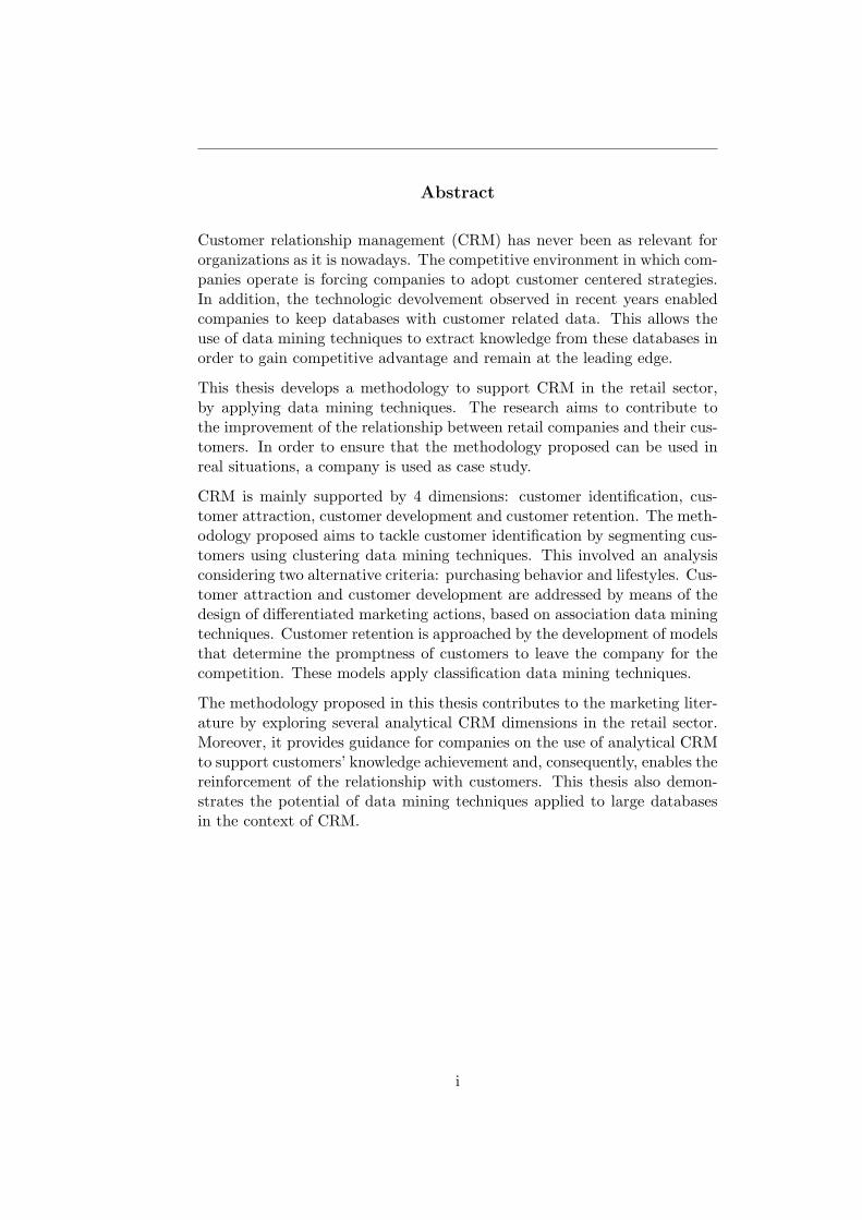
Abstract
Customer relationship management (CRM) has never been as relevant fororganizations as it is nowadays. The competitive environment in which com-panies operate is forcing companies to adopt customer centered strategies.In addition, the technologic devolvement observed in recent years enabledcompanies to keep databases with customer related data. This allows theuse of data mining techniques to extract knowledge from these databases inorder to gain competitive advantage and remain at the leading edge.
This thesis develops a methodology to support CRM in the retail sector,by applying data mining techniques. The research aims to contribute tothe improvement of the relationship between retail companies and their cus-tomers. In order to ensure that the methodology proposed can be used inreal situations, a company is used as case study.
CRM is mainly supported by 4 dimensions: customer identification, cus-tomer attraction, customer development and customer retention. The meth-odology proposed aims to tackle customer identification by segmenting cus-tomers using clustering data mining techniques. This involved an analysisconsidering two alternative criteria: purchasing behavior and lifestyles. Cus-tomer attraction and customer development are addressed by means of thedesign of differentiated marketing actions, based on association data miningtechniques. Customer retention is approached by the development of modelsthat determine the promptness of customers to leave the company for thecompetition. These models apply classification data mining techniques.
The methodology proposed in this thesis contributes to the marketing liter-ature by exploring several analytical CRM dimensions in the retail sector.Moreover, it provides guidance for companies on the use of analytical CRMto support customers’ knowledge achievement and, consequently, enables thereinforcement of the relationship with customers. This thesis also demon-strates the potential of data mining techniques applied to large databasesin the context of CRM.
i

ii
Resumo
O Customer relationship management (CRM) nunca foi tao crucial para asempresas como e atualmente. O ambiente competitivo em que as empresasoperam tem imposto a adocao de estrategias centradas no cliente. Paraalem dito, o desenvolvimento tecnologico verificado nos ultimos anos tempermitido as empresas manter bases de dados com informacoes relativasaos clientes. Isto permite o uso de tecnicas de data mining para extrairconhecimento dessas bases de dados de forma a obter vantagens competitivase a ocupar posicoes de lideranca.
Esta tese desenvolve uma metodologia de suporte ao CRM no sector deretalho, usando tecnicas de data mining. A investigacao visa contribuir paraa melhoria da relacao entre as grandes empresas de retalho e os seus clientes.De forma a assegurar que os metodos propostos possam ser aplicados emsituacoes reais usa-se uma empresa como caso de estudo.
O CRM baseia-se essencialmente em 4 dimensoes: a identificacao, a atracao,o desenvolvimento e a retencao dos clientes. A metodologia proposta temcomo objetivo abordar a identificacao dos clientes recorrendo a tecnicas declustering. Isto envolveu uma analise considerando dois criterios alterna-tivos: o comportamento de compra e o estilo de vida. A atracao e o de-senvolvimento dos clientes sao abordados atraves do desenho de acoes demarketing diferenciadas, baseadas em tecnicas de associacao. A retencaodos clientes e abordada atraves do desenvolvimento de modelos de identi-ficacao dos clientes que poderao vir a abandonar a empresa. Estes modelosbaseiam-se em tecnicas de classificacao.
A metodologia proposta nesta tese contribui para a literatura de marketingatraves da analise de diferentes dimensoes do CRM analıtico no sector doretalho. Para alem dito, a metodologia serve como guia as empresas de comoo CRM analıtico pode suportar a extracao de conhecimento e como conse-quentemente pode contribuir para a melhoria da sua relacao com os clientes.O trabalho desenvolvido tambem demonstra o potencial das tecnicas de datamining aplicadas a grandes bases de dados no contexto do CRM.
iii

iv

Acknowledgments
My first thanks goes to Prof. Ana Camanho, whose supervision was crucialfor my doctoral work. Thanks for her time and for sharing her knowledge. Ialso thank Prof. Joao Falcao e Cunha for all comments on my work. I thankProf. Dirk Van den Poel for welcoming me in the UGent and for providingme very good working conditions. I also thank my UGent colleagues fortheir hospitality, help and friendship.
I would like to express my gratitude to the company used as case studyand its collaborators, particularly to Dr. Nuno and to Dr. Ana Paula, forproviding the data and all necessary information. Thanks for the economicsupport. It enabled the discussion of the research work by the domainexperts.
I also thank the Portuguese Foundation for Science and Technology (FCT)for my grant (SFRH/BD/60970/2009) cofinanced by POPH - QREN “Tipolo-gia” 4.1 Advanced Formation, and co-financed by Fundo Social Europeuand MCTES.
I thank my colleges and friends from the Industrial Engineering departmentfor all moments of fun over the last years, particularly: Andreia Zanella,Isabel Horta, Joao Mourinho, Luıs Certo, Marta Rocha, Paulo Morais, PedroAmorim and Rui Gomes. Marta, I will miss you a lot! I also thank theProfessors I have worked with, namely Prof. Ana Camanho, Prof. JoseFernando Oliveira, Prof. Maria Antonia Carravilla and Prof. Pina Marques,for all support concerning all teaching tasks. I also thank Prof. SarsfieldCabral, head of the department, for his encouragement over these years. Iacknowledge D. Soledade, Isabel and Monica for all nice chats and friendship.
Finally I thank all my family for the support, specially my parents, mybrother and my grandmother. I thank all my friends for all moments of fun,which provided me energy to conduct this project. I also thank Andre forhis company, help, comprehension and love.
v
Acronyms
ANN Artificial Neural Networks
AUC Area Under Curve
CART Classification And Regrets Techniques
CLV Clustering around Latent Variables
CRM Customer Relationship Management
DIY Do It Yourself
DVD Digital Video Device
EM Expectation Maximization
ERP Enterprise Resource Planning
EU European Union
GDP Gross Domestic Product
ID3 Iterative Dichotomiser3
IT Information Technology
KDD Knowledge Discovery in Databases
MBA Market Basket Analysis
PCC Percentage Correctly Classified
POS Point Of Sale
RFM Recency Frequency and Monetary
RM Relationship Marketing
ROC Receiver Operating Characteristic
SOM Self-Organizing Map
VIF Variance Inflation Factor
VLMC Variable Length Markov Chains
WOM Word-Of-Mouth
vi
Table of Contents
Abstract i
Resumo iii
Acknowledgements v
Table of Contents vii
List of Figures xi
List of Tables xiii
1 Introduction 1
1.1 General context . . . . . . . . . . . . . . . . . . . . . . . . . . 1
1.2 Research motivation and general objective . . . . . . . . . . . 3
1.3 Specific objectives . . . . . . . . . . . . . . . . . . . . . . . . 4
1.4 Thesis outline . . . . . . . . . . . . . . . . . . . . . . . . . . . 6
2 Customer Relationship Management 9
2.1 Introduction . . . . . . . . . . . . . . . . . . . . . . . . . . . . 9
2.2 Marketing concept . . . . . . . . . . . . . . . . . . . . . . . . 9
2.3 Customer relationship management concept . . . . . . . . . . 12
2.3.1 CRM benefits . . . . . . . . . . . . . . . . . . . . . . . 13
2.3.2 CRM components . . . . . . . . . . . . . . . . . . . . 14
2.4 Analytical CRM . . . . . . . . . . . . . . . . . . . . . . . . . 16
vii
TABLE OF CONTENTS
2.4.1 Dimensions . . . . . . . . . . . . . . . . . . . . . . . . 16
2.4.2 Applications . . . . . . . . . . . . . . . . . . . . . . . 19
2.5 Summary and conclusions . . . . . . . . . . . . . . . . . . . . 22
3 Introduction to data mining techniques 25
3.1 Introduction . . . . . . . . . . . . . . . . . . . . . . . . . . . . 25
3.2 Knowledge discovery . . . . . . . . . . . . . . . . . . . . . . . 26
3.3 Data mining and analytical CRM . . . . . . . . . . . . . . . . 29
3.4 Clustering . . . . . . . . . . . . . . . . . . . . . . . . . . . . . 34
3.4.1 Partitioning methods . . . . . . . . . . . . . . . . . . . 36
3.4.2 Model-based methods . . . . . . . . . . . . . . . . . . 38
3.4.3 Hierarchical methods . . . . . . . . . . . . . . . . . . . 45
3.4.4 Variable clustering methods . . . . . . . . . . . . . . . 49
3.5 Classification . . . . . . . . . . . . . . . . . . . . . . . . . . . 49
3.5.1 Logistic regression . . . . . . . . . . . . . . . . . . . . 50
3.5.2 Decision trees . . . . . . . . . . . . . . . . . . . . . . . 51
3.5.3 Random forests . . . . . . . . . . . . . . . . . . . . . . 58
3.5.4 Neural networks . . . . . . . . . . . . . . . . . . . . . 59
3.6 Association . . . . . . . . . . . . . . . . . . . . . . . . . . . . 63
3.6.1 Apriori algorithm . . . . . . . . . . . . . . . . . . . . . 65
3.6.2 Frequent-pattern growth . . . . . . . . . . . . . . . . . 66
3.7 Conclusion . . . . . . . . . . . . . . . . . . . . . . . . . . . . 68
4 Case study: description of the retail company 71
4.1 Introduction . . . . . . . . . . . . . . . . . . . . . . . . . . . . 71
4.2 Company’s description . . . . . . . . . . . . . . . . . . . . . . 71
4.3 Loyalty program . . . . . . . . . . . . . . . . . . . . . . . . . 73
4.4 Customers characterization . . . . . . . . . . . . . . . . . . . 75
4.5 Conclusion . . . . . . . . . . . . . . . . . . . . . . . . . . . . 79
viii
TABLE OF CONTENTS
5 Behavioral market segmentation to support differentiatedpromotions design 81
5.1 Introduction . . . . . . . . . . . . . . . . . . . . . . . . . . . . 81
5.2 Review of segmentation and MBA context . . . . . . . . . . . 82
5.3 Methodology . . . . . . . . . . . . . . . . . . . . . . . . . . . 85
5.3.1 Segmentation . . . . . . . . . . . . . . . . . . . . . . . 85
5.3.2 Products association . . . . . . . . . . . . . . . . . . . 86
5.4 Behavioral segments and differentiated promotions . . . . . . 87
5.5 Conclusion . . . . . . . . . . . . . . . . . . . . . . . . . . . . 92
6 Lifestyle market segmentation 93
6.1 Introduction . . . . . . . . . . . . . . . . . . . . . . . . . . . . 93
6.2 Methodology . . . . . . . . . . . . . . . . . . . . . . . . . . . 94
6.3 Lifestyle segments . . . . . . . . . . . . . . . . . . . . . . . . 95
6.4 Marketing actions . . . . . . . . . . . . . . . . . . . . . . . . 103
6.5 Conclusion . . . . . . . . . . . . . . . . . . . . . . . . . . . . 105
7 Partial customer churn prediction using products’ first pur-chase sequence 107
7.1 Introduction . . . . . . . . . . . . . . . . . . . . . . . . . . . . 107
7.2 Customers retention . . . . . . . . . . . . . . . . . . . . . . . 108
7.3 Churn prediction modeling . . . . . . . . . . . . . . . . . . . 109
7.4 Methodology . . . . . . . . . . . . . . . . . . . . . . . . . . . 112
7.4.1 Partial churning . . . . . . . . . . . . . . . . . . . . . 113
7.4.2 Explanatory variables . . . . . . . . . . . . . . . . . . 114
7.4.3 Evaluation criteria . . . . . . . . . . . . . . . . . . . . 118
7.5 Partial churn prediction model and retention actions . . . . . 119
7.6 Conclusion . . . . . . . . . . . . . . . . . . . . . . . . . . . . 124
ix
TABLE OF CONTENTS
8 Partial customer churn prediction using variable length prod-ucts’ first purchase sequences 125
8.1 Introduction . . . . . . . . . . . . . . . . . . . . . . . . . . . . 125
8.2 Variable length sequences . . . . . . . . . . . . . . . . . . . . 126
8.3 Methodology . . . . . . . . . . . . . . . . . . . . . . . . . . . 126
8.3.1 Evaluation criteria . . . . . . . . . . . . . . . . . . . . 127
8.3.2 Explanatory variables . . . . . . . . . . . . . . . . . . 128
8.4 Partial churn prediction model . . . . . . . . . . . . . . . . . 129
8.5 Conclusion . . . . . . . . . . . . . . . . . . . . . . . . . . . . 132
9 Conclusions 133
9.1 Introduction . . . . . . . . . . . . . . . . . . . . . . . . . . . . 133
9.2 Summary and conclusions . . . . . . . . . . . . . . . . . . . . 133
9.3 Contributions of the thesis . . . . . . . . . . . . . . . . . . . . 137
9.4 Directions for future research . . . . . . . . . . . . . . . . . . 138
A Appendix 141
References 144
x
List of Figures
2.1 Analytical CRM stages. (Kracklauer et al., 2004) . . . . . . . 17
2.2 CRM instruments. (Kracklauer et al., 2004) . . . . . . . . . . 19
3.1 Overview of the stages constituting the KDD process. (Fayyadet al., 1996b) . . . . . . . . . . . . . . . . . . . . . . . . . . . 27
3.2 Typical effort needed for each stage of the KDD process (Cabenaet al., 1997). . . . . . . . . . . . . . . . . . . . . . . . . . . . . 29
3.3 Classification framework on data mining techniques in CRM.(Ngai et al., 2009) . . . . . . . . . . . . . . . . . . . . . . . . 33
3.4 Illustrative example of a clustering result. (Berry and Linoff,2004) . . . . . . . . . . . . . . . . . . . . . . . . . . . . . . . . 35
3.5 Kohonen map. (Yin et al., 2011) . . . . . . . . . . . . . . . . 41
3.6 Probabilistic hierarchical tree. (Han and Kamber, 2006) . . . 44
3.7 Dendrogram example. (Hromic et al., 2006) . . . . . . . . . . 45
3.8 Single linkage distance. . . . . . . . . . . . . . . . . . . . . . . 47
3.9 Complete linkage distance. . . . . . . . . . . . . . . . . . . . . 47
3.10 Average linkage distance. . . . . . . . . . . . . . . . . . . . . 48
3.11 Example of a decision tree concerning the purchase of a com-puter. (Han and Kamber, 2006) . . . . . . . . . . . . . . . . . 52
3.12 Random forests.(Tan et al., 2006) . . . . . . . . . . . . . . . . 58
3.13 Neuron architecture. (McCulloch and Pitts, 1990) . . . . . . 60
3.14 Most common activation functions.(Negnevitsky, 2004) . . . . 60
3.15 Single Layer Feed-forward Network example. . . . . . . . . . 60
3.16 Multiple Layer Feed-forward Network example. . . . . . . . . 61
xi
LIST OF FIGURES
3.17 Recurrent Network example. . . . . . . . . . . . . . . . . . . . 61
3.18 Apriori algorithm. (Rajaraman and Ullman, 2011) . . . . . . 66
3.19 FP-tree example. . . . . . . . . . . . . . . . . . . . . . . . . . 67
4.1 Histogram of the average amount of money spent per trans-action. . . . . . . . . . . . . . . . . . . . . . . . . . . . . . . . 77
4.2 Histogram of the average time between purchases. . . . . . . 78
4.3 Distribution of the number of transactions per business unit. 78
4.4 Distribution of the amount spent per business unit. . . . . . . 79
5.1 Error measures for different numbers of clusters. . . . . . . . 88
5.2 Clusters characterization. . . . . . . . . . . . . . . . . . . . . 89
6.1 Products’ dendrogram resulting from the varclus algorithm. . 96
6.2 Proportion of products in each business unit. . . . . . . . . . 97
6.3 Proportion of products in the main category. . . . . . . . . . 99
6.4 Proportion of products in each brand position. . . . . . . . . 100
7.1 Examples of the derivation of a partial churning indicator. . . 114
xii
List of Tables
3.1 Set of transactions. . . . . . . . . . . . . . . . . . . . . . . . . 66
5.1 Association rules for Cluster 4. . . . . . . . . . . . . . . . . . 90
5.2 Association rules for Cluster 0. . . . . . . . . . . . . . . . . . 91
6.1 Number of products in each cluster. . . . . . . . . . . . . . . 96
6.2 Relevant categories. . . . . . . . . . . . . . . . . . . . . . . . 98
6.3 Distribution of customers by the clusters. . . . . . . . . . . . 103
6.4 Distribution of customers by the clusters for specific stores. . 105
7.1 Performance results. . . . . . . . . . . . . . . . . . . . . . . . 122
8.1 Forward model - first stage sequences selection. . . . . . . . . 130
8.2 Backward model - first stage sequences selection. . . . . . . . 130
8.3 Performance results. . . . . . . . . . . . . . . . . . . . . . . . 131
A1 Non-churners transition matrix. . . . . . . . . . . . . . . . . . 142
A2 Churners transition matrix. . . . . . . . . . . . . . . . . . . . 143
xiii

LIST OF TABLES
xiv
Chapter 1
Introduction
1.1 General context
Retailing is an activity that involves buying goods or services and subse-
quently selling them to the final consumer, usually in small quantities and
without transformation. A retailer is a reseller, i.e., obtains a product or
service from someone in order to sell to others. Retail services encompass a
wide variety of forms (shops, electronic commerce, open markets, etc.), for-
mats (small shops, supermarkets, hypermarkets, etc.), products (food, non-
food, prescription, over-the-counter drugs, etc.), legal structures (indepen-
dent stores, franchises, integrated groups, etc.), and locations (urban/rural,
city centre/suburbs, etc.).
The retail sector is vital to the world economy, as it provides large scale
employment to skilled and unskilled labor, casual, full-time and part-time
workers. In 2008 the retail sector employed a total of 17.4 million people in
the EU (8.4% of the total EU workforce). The economic significance of this
sector for the European Union is also revealed by its GDP share, i.e. 4.2%
of the EU’s GDP in 2008 (European Commission, 2008).
According to Malonis (1999), in the late 18th century in Europe, the diver-
1
Chapter 1. Introduction
sity of goods and the existence of people with disposable income to purchase
those goods enabled the emergence of a merchant class and numerous shops.
Mass retailing began to emerge in the second half of the 19th century when
improvements in manufacturing compelled merchants to build stores that
could sell a wide range of products in high volume. Merchants in west-
ern Europe created department stores, i.e. the first mass-retailing outlets.
These stores were mainly located in city centres. This growing pattern con-
tinued well into the 20th century with a cluster of stores downtown that sold
many goods, and a few food and general merchandise stores in the neighbor-
hoods. The last decades have been mainly characterized by the emergence
of electronic commerce. Moreover, these decades have been marked by the
consolidation and rise of large store chains to replace smaller or local ones.
This trend has occurred earlier in the grocery context, with the well-known
supermarket revolution, which drove many smaller and traditional grocery
retailers out of business. A parallel movement was the rise of the so-called
category killer stores. This type of stores offers a very wide selection of
items in its market category and sometimes at lower prices than smaller
retailers. In theory, category killers eliminate the necessity of consumers
to shop around for a particular item of interest because these stores carry
almost everything. Both category killer and superstore formats have been
adopted in diverse areas, such as hardware, office suppliers, consumer elec-
tronics, books and home decoration.
Currently the retail sector growth is slowing down. Therefore, companies
are competing intensely for market share. Price is one of the most important
competitive dimensions. In addition, loyalty actions, enabled by the imple-
mentation of loyalty programs, are also considered an extremely important
dimension of competitiveness.
Besides the changes in the form and competition in retailing, the evolution
of information technology (IT) also enabled a significant reduction of lo-
2
1.2 Research motivation and general objective
gistic and store operation costs. Relevant advances in retailer’s operation
is enabled by the electronic information technology, where bar-coding and
electronic scanning of products play a central role.
1.2 Research motivation and general objective
Due to the increased competitiveness of the retail activity, the relationship
between companies and customers became a critical factor of companies’
strategy. In the past, companies focused on selling products and services
without searching detailed knowledge concerning the customers who bought
the products and services. With the proliferation of competitors, it became
more difficult to attract new customers, and consequently companies had to
intensify efforts to keep current consumers. The evolution of social and eco-
nomic conditions also changed lifestyles, and as a result customers became
less inclined to answer positively to all marketing communications from com-
panies. This context led companies to evolve from product/service-centered
strategies to customer-centered strategies. Therefore, the establishment of
loyal relationships with customers became a main strategic goal. Indeed,
companies wishing to be at the leading edge have to improve continuously
the service levels, in order to ensure a good business relationship with cus-
tomers.
Some companies invested in creating databases that are able to store a big
amount of customer-related data. For each customer, many data objects are
collected, allowing the analysis of the complete customers’ purchasing his-
tory. However, the information obtained is seldom integrated in the design
of business functions such as customer relationship management (CRM).
In fact, in most companies, the information available is not integrated in
procedures to support decision making. The overwhelming amounts of data
have often resulted in the problem of information overload but knowledge
3
Chapter 1. Introduction
starvation. Analysts have not being able to keep pace to study the data and
turn it into useful knowledge for application purposes.
In this context, the doctoral work described in this thesis aims to develop a
methodology to support CRM in the retail sector, such that the relationship
between companies and their customers can be reinforced. This research
focuses on customer identification, attraction, development and retention.
The research applies data mining techniques to extract knowledge from large
databases.
In this thesis, a food-based retail company is used as case study, in order
to ensure that the methods and models proposed can be applied to real
contexts.
1.3 Specific objectives
This section summarizes the specific research objectives. These objectives
are linked to the chapters of the thesis and consequently, for each objective,
the corresponding thesis chapter is indicated.
Taking into account that a retail company receives thousands of visits to its
stores every day, it is not possible to know each customer personally. There-
fore, from a managerial point of view, companies are not able to customize
their relationship with each customer. In order to establish and reinforce the
relationship with customers, companies need to identify groups of customers
who can be treated similarly. This procedure allows companies to structure
the knowledge concerning the customers, and to define the target market
for specific marketing actions. According to companies’ goals, several mod-
els of segmentation can be developed. The methodology proposed in this
thesis aims to construct a segmentation model based on customers’ shop-
ping behavior, namely the frequency of visits to the stores and the amount
4
1.3 Specific objectives
spent. Having segmented the market, it is of utmost importance to endure
the relationship with customers from specific market segments. Therefore,
the methodology also intends to support the design of differentiated mar-
keting actions to encourage customers from different segments to visit the
stores more often and spend more on purchases. This involves promoting
the purchase of different kinds of products, that are still not purchased by
the clients despite their potential interest. From a technical point of view,
this thesis aims to use market basket analysis within clusters to discover
frequent associations between products (Chapter 5).
The research aims to explore other forms of segmentation. The methodology
proposed in this thesis aims to construct a segmentation model based on the
content of customers’ shopping baskets. This methodology intends to infere
customers’ lifestyle from the content of their shopping baskets and to give
insights into the most appropriate products to promote for each segment of
customers (Chapter 6).
Considering that attracting new customers is more costly than retaining
current customers, it is important to take measures to avoid customers de-
fection. The methodology developed in this thesis aims to construct a model
able to identify the new customers who will leave the company. The research
intends to explore the use of a similarity measure of the sequences of the
first products purchased with the sequences observed for churners and non-
churners. The methodology aims to support the decision makers in directing
their marketing efforts to those customers who are more prone to leave the
company (Chapter 7).
The methodology proposed also aims to explore the use of variable length
sequences of the first products purchased to identify the new customers who
will leave the company. The research intends to analyze these sequences
ordered in chronological order and in reverse chronological order (Chapter
5
Chapter 1. Introduction
8).
In order to make the methodology applicable to large databases, this thesis
applied data mining techniques.
1.4 Thesis outline
This thesis includes 9 chapters, which are summarized below.
Chapter 2 presents a summary of the literature regarding marketing and
customer relationship management concepts. This chapter aims to introduce
the main topics covered in this thesis and to revise some existing studies
centered on customer relationship marketing, in order to provide insights
into the research directions addressed.
Chapter 3 provides a summary of knowledge discovery processes, giving em-
phasis to the data mining stage. It presents the main data mining techniques
used to support analytical CRM, in order to give insights into the techniques
that could have been used in the doctoral work.
Chapter 4 describes the retail company used as a case study. This chapter
contains a description of the company position in the market, store formats,
organizational structure and products classification. In addition, it includes
a brief presentation of the loyalty program, segmentation models and pro-
motional policies conducted by the company. This chapter also includes a
brief characterization of the company’s customers.
Chapter 5 proposes a method for customers’ behavioral segmentation, based
on the frequency of visits and monetary value spent. This is achieved by
using k -means. This chapter also proposes a model to characterize the
customers’ profile within each segment, by means of a decision tree. This
chapter also includes a model to identify product associations within seg-
ments, which can base the identification of products which can be part of
6
1.4 Thesis outline
differentiated promotions. This is done by means of the apriori algorithm.
Chapter 6 presents a model for market segmentation based on customers’
lifestyle. By using the varclus algorithm, this method identifies a group
of typical shopping baskets, which are used to infer customers’ lifestyle.
Customers can then be allocated to a specific lifestyle segment based on
their purchase history.
Chapter 7 develops a model to address customers retention. This model
(i.e. a churn prediction model) estimates the probability of a new customer
leaving the company for the competition using random forests and logistic
regression. This model uses as a predictor the similarity of the sequences
of the first products purchased with churner’s and non-churner’s sequences.
The sequence of first purchase events is modeled by means of markov-for-
discrimination.
Chapter 8 proposes additional models to support customers’ retention. These
models explore the use of variable length sequences of the first products pur-
chased as predictors. These sequences are modeled in chronological order
and in reverse chronological order. These models are supported by a logistic
regression.
Chapter 9 presents the summary and conclusions of the research developed
in this thesis. It also lists the main contributions of the thesis and presents
some directions for future research.
7

Chapter 1. Introduction
8
Chapter 2
Customer RelationshipManagement
2.1 Introduction
This chapter provides a revision of the concepts of marketing and customer
relationship management. The objective of this chapter is to introduce the
main topics approached in this thesis in order to contextualize the research
objectives. It also provides a brief literature review on CRM.
This chapter is structured as follows. Section 2.2 presents the evolution of
the marketing concept over time, giving particular attention to the concept
of relationship marketing. Section 2.3 consists of an overview of the con-
cept, benefits and components of CRM. Section 2.4 gives emphasis to the
dimensions and applications of analytical CRM. Section 2.5 summarizes and
concludes.
2.2 Marketing concept
The initial concept of marketing focused on the process through which goods
and services moved from suppliers to consumers. It emerged in the transition
9
Chapter 2. Customer Relationship Management
from a purely subsistence-based society, in which families produced their own
goods, to more cooperative and specialized forms of the civilization. For
instance, the simple act of trading a tool for cereals entails some marketing
aspects. The term marketing derives from the word market, which means a
group of sellers and buyers that cooperate to exchange goods and services.
Some researchers have divided the history of marketing into four distinct
eras, corresponding to different practices and focus (Hollander et al., 2005;
Boone and Kurtz, 2008). The periods commonly cited include, in chrono-
logical order, the production era, the sales era, the marketing era, and the
relationship era.
The production era predates the second world war. The main emphasis of
marketing consisted of producing a satisfactory product, without big efforts,
and introducing it to the potential customers, through catalogs, brochures
and advertising. The sales era ran from the 30s to the 50s and promoted
the concept of transactional marketing. Due to the excess of supply over
demand, companies recognized the need of having salespeople to sell the
products. The marketing emphasis was placed on developing persuasive ar-
guments to encourage customers to buy the products. By the 1950s, and
until the 1960s, this context evolved further into the marketing era, when
companies began to adopt a customer orientation and became aware of the
importance of following consumer preferences and motivations. Finally, the
relationship era as well as the marketing concept as it is known nowadays
had its origin in 1980s. This was a period of technological and scientific
progresses which resulted in mass manufacturing. This fact, combined with
the development of transport systems and mass media, namely the radio,
promoted the management of the sales of goods. It created a separation
between companies and their customers, since it was no longer feasible for
companies to customize their products. Therefore, companies were no longer
able to personally know their clients. There was practically no interaction
10
2.2 Marketing concept
between customers and companies. The concept of relationship market-
ing (RM), proposed by Berry (1983), arose as an attempt to minimize the
gap between companies and their customers. RM is not focused on simple
transactions but on retaining customers and facilitating more complex long
term relationships with customers. Berry’s notion of relationship marketing
resembles the ideas of other scholars studying services marketing, such as
Levitt (1981), Gronroos (1983) and Gummesson (1987).
According to Sheth (2002) there are three main events that aroused the
interest of companies in RM. First, the energy crises of 1970 and the conse-
quent economic inflation resulted in the reduction of raw materials’ demand,
which caused surplus inventories. These facts obliged companies to evolve
from marketing approaches, based on transactional marketing, to relation-
ship marketing, giving emphasis on retaining customers (Sheth et al., 1988).
Second, research started to be focused on the distinctive aspects of services
marketing and product marketing techniques, what resulted in the emer-
gence of RM concept. Third, product quality became an important issue
for companies, which started launching new programs to establish stronger
relationships with their suppliers in order to better manage, improve and
control quality. Sheth (2002) also considers three other factors that later
influenced the definition of relationship marketing. First, internet and IT,
such as enterprise resource planning (ERP) systems, allowed companies to
focus on customer relationship management. Second, the emergence of the
belief that companies should be selective and target their relationships pro-
moted a new vision of marketing. Finally, the theory of Sheth and Sisodia
(1999) which stated that customers outsourcing should be implemented to
deal with non-profitable customers also conduced to the current relationship
marketing concept.
Currently, there are several definitions of the RM concept (see Harker, 1999,
for an overview). According to Gronroos (1990), RM consists of identify-
11
Chapter 2. Customer Relationship Management
ing, establishing, maintaining and enhancing long-term relationships with
customers and other stakeholders at a profit, so that the objectives of the
parties involved are met. This is done by mutual exchange and fulfilment of
promises. Gronroos (1990) also claims that RM should consider the extinc-
tion of the relationships with the customers when this is convenient. Coviello
et al. (1997) defines relationship marketing as an integrative activity involv-
ing functions across the organization, with emphasis on facilitating, building
and maintaining relationships over time.
2.3 Customer relationship management concept
CRM is based on RM and is focused on the technology underlying the man-
agement of customers. CRM has its origin in the desire of combining the
help desk, the customer support, the ERP and data mining (Peel, 2002).
The first CRM initiatives were launched in the early 1990s and were mainly
focused on call center activities (Roya Rahimi, 2007). The promising emer-
gence of CRM was influenced by the advances in information technologies,
data management systems, improved analytics, enhanced communications,
systems integration and internet adoption (Greenberg, 2001). Currently, in
information technology terms, CRM means the integration of technologies
such as: datawarehouse, website, intranet/extranet, help desk, sales, ac-
counting, ERP and data mining. Indeed, all information technology able
to gather data is integrated in order to provide the information required to
create a more personal interaction with customers (Bose, 2002).
CRM can be defined as the process of using information technology in im-
plementing relationship marketing strategies, with particular emphasis on
customer relationships (Ryals and Payne, 2001; Gummesson, 2008). Nairn
(2002) goes further and defines CRM as a long-term business philosophy that
focuses on collecting and understanding customer information, treating dif-
12
2.3 Customer relationship management concept
ferent customers differently, providing a higher level of service for the best
customers and using these together to increase customer loyalty and prof-
itability. This is further supported by Buttle (2003) who states that CRM
is a core business strategy that combines internal processes and functions
with external networks to create and deliver value to targeted customers at
a profit. Buttle (2003) also highlights the importance of using high-quality
customer data. Other CRM definitions can be found in the literature (see
Payne and Frow, 2005; Ngai, 2005, for an overview).
2.3.1 CRM benefits
Although most benefits of CRM are different in each business area, there
are some benefits common to all businesses (Swift, 2000). These benefits are
generally the following: lower cost of customers’ acquisition, improvement
of customer services, customer retention and loyalty increase, higher cus-
tomers profitability, easier identification of profitable customers and com-
panies’ productivity increase (Alhaiou, 2011). The cost of customers ac-
quisition decreases due to the possibility of saving on marketing, mailing,
contact, follow-up, fulfilment services and so on (Swift, 2000; Romano and
Fjermestad, 2003; Curry and Kkolou, 2004). Customer service improves
due to the analysis of processes promoted by CRM. The data integration
and the knowledge sharing with all dealers incites the design of customized
processes, what stimulates increased levels of service (Fjermestad et al.,
2006). As a consequence of customer service improvement, customers satis-
faction increases and customers stay longer. Moreover, loyalty increases be-
cause companies can use customers’ knowledge to develop loyalty programs
(Crosby, 2002; Swift, 2000; Curry and Kkolou, 2004). Regarding customers’
profitability, it increases due to the increase of up-selling, cross-selling and
followup sales (Bull, 2003; Curry and Kkolou, 2004). Companies are able
to know which customers are profitable, which are going to be profitable in
13
Chapter 2. Customer Relationship Management
the future and which ones will never be profitable by the analysis of cus-
tomers’ data (Kotler, 1999; Swift, 2000; Curry and Kkolou, 2004). CRM
also promotes the increase of companies’ productivity since it enables the
integration of all companies’ departments, such as information technology,
finance and human resources (Romano and Fjermestad, 2003; Crosby, 2002;
Kracklauer et al., 2001).
2.3.2 CRM components
According to Dych (2001), the CRM technologies can be divided in three
components: operational, collaborative and analytical.
Operational CRM referees to the component that helps improving the ef-
ficiency of day-to-day customers operations (Peppers and Rogers, 2011).
Therefore, this is concerned with the automation of processes involving com-
munication and interaction with customers and integrates front, back and
mobile offices. This CRM component is the initial producer of data and in-
cludes typical corporate functions of sales automation, enterprise marketing
automation, order management and customer service or support (Crosby
and Johnson, 2001; Greenberg, 2004). In order to ensure success of opera-
tional CRM, companies should focus on the requirements of customers and
employees should have the right skills to satisfy customers. The output from
operational CRM solutions typically are summary level only, showing what
activities occurred, but failing to explain their causes or impact (Reynolds,
2002).
Collaborative CRM can be seen as a communication centre that provides
the connection between companies and their customers, suppliers, and busi-
ness partners. Indeed, it allows customers, staff, sales people and partners
to access, distribute and share data. Personalized publishing, e-mail, com-
munities, conferences and web-enabled relationship interaction centres are
14
2.3 Customer relationship management concept
examples of collaborative services. These services make teamwork easier and
more productive, enabling companies to improve processes and consequently
improve customers’ satisfaction (Greenberg, 2001). Collaborative CRM is
used to establish the lifetime value of customers beyond the transaction by
creating a partnering relationship.
In the past, companies focused on operational and collaborative tools, but
this tendency seems to be changing (Reynolds, 2002). Decision-makers have
realized that analytical tools are necessary to drive strategy and tactical deci-
sions, related to customer identification, attraction, development and reten-
tion. Analytical CRM is mainly focused on analyzing the data collected and
stored, in order to create more meaningful and profitable interactions with
customers. To achieve this purpose the data is processed, interpreted and
reported using several tools (Greenberg, 2004). The data analyzed is part
of a large reservoir of information, i.e. a data warehouse, which contains
data from both external and internal sources, obtained using operational
tools. The data gains value when the knowledge extracted becomes action-
able. According to Reynolds (2002), the most critical CRM component is
the analysis. Analytical CRM solutions allow to manage effectively the re-
lationship with customers. Only by analyzing customers data, companies
can understand behaviors, identify buying patterns and trends and discover
causal relationships. The insights obtained from the data help to model and
predict future customer satisfaction and behavior more accurately, and may
constitute a quantified foundation for strategic decision making.
According to Reynolds (2002), each CRM component is dependent on the
others. For instance, analytics drives the decision making in operational
CRM, e.g. sales arrangement, marketing actions and customer service pro-
cesses. On the other hand, without the data collected via operational CRM
processes, analytical CRM would not be possible. Moreover, the data pro-
cessed by analytical CRM tools could not be used effectively and strategic
15
Chapter 2. Customer Relationship Management
decision-making would not occur without collaborative CRM. Summing up,
operational CRM, collaborative CRM and analytical CRM work together to
create business value.
2.4 Analytical CRM
The doctoral work described in this thesis is mainly concerned about ana-
lytical CRM since it aims to explore the use of data mining techniques to
improve the relationship between companies and their customers. Therefore,
this section explores in more detail analytical CRM, namely its dimensions
and applications.
2.4.1 Dimensions
Following Swift (2000); Parvatiyar and Sheth (2002); Kracklauer et al. (2004),
Ngai et al. (2009) categorizes analytical CRM on four dimensions: (1) cus-
tomer identification, (2) customer attraction, (3) customer development and
(4) customer retention. These four dimensions can be seen as a closed cycle
of the customers management system (Au et al., 2003; Kracklauer et al.,
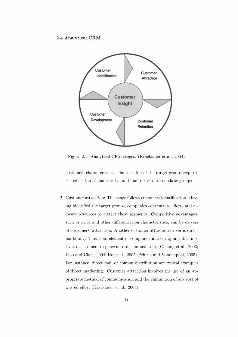
2004; Ling and Yen, 2001). The diagram of Figure 2.1 shows the sequence
of relevant components of CRM.
These four CRM dimensions can be described as follows:
1. Customer identification: CRM begins with this dimension, also called
customer acquisition (Kracklauer et al., 2004). Customer identification
includes mainly customer segmentation and target customer analysis.
Customer segmentation implies the subdivision of the set of all cus-
tomers into smaller segments including customers with similar char-
acteristics (Woo et al., 2005). Target customer analysis involves the
definition of the most attractive segments for the company, based on
16
2.4 Analytical CRM
Figure 2.1: Analytical CRM stages. (Kracklauer et al., 2004)
customers characteristics. The selection of the target groups requires
the collection of quantitative and qualitative data on these groups.
2. Customer attraction: This stage follows customers identification. Hav-
ing identified the target groups, companies concentrate efforts and al-
locate resources to attract these segments. Competitive advantages,
such as price and other differentiation characteristics, can be drivers
of customers’ attraction. Another customer attraction driver is direct
marketing. This is an element of company’s marketing mix that mo-
tivates customers to place an order immediately (Cheung et al., 2003;
Liao and Chen, 2004; He et al., 2005; Prinzie and Vandenpoel, 2005).
For instance, direct mail or coupon distribution are typical examples
of direct marketing. Customer attraction involves the use of an ap-
propriate method of communication and the elimination of any sort of
wasted effort (Kracklauer et al., 2004).
17
Chapter 2. Customer Relationship Management
3. Customer development: The main focus of this dimension is to increase
transaction intensity, transaction value, and individual customer prof-
itability. The main elements of customer development are customer
lifetime value analysis and up/cross selling. Customer lifetime value
is the total net income that a company can expect from a customer
(Drew et al., 2001; Rosset et al., 2003). Up/Cross selling are the
promotional activities that aim to increase the number of associated
or closely related services or products that a customer uses within a
company (Prinzie and Van den Poel, 2006). The design of such promo-
tional activities is usually supported by market basket analysis, which
allows to identify the patterns underlying customer behavior (Aggar-
wal et al., 2002; Giraud-Carrier and Povel, 2003; Kubat et al., 2003).
4. Customer retention: This dimension is one of the main concerns of
CRM. According to Kracklauer et al. (2004), customer satisfaction is
the main issue regarding customers retention. Customer satisfaction
can be defined as the comparison of customers expectations (resulting
from personal standard, image of the company, knowledge of alter-
natives, etc) with the perceptions (resulting from actual experience,
subjective impression of product performance, appropriateness of the
product or service, etc). The customer’s perception of the value offered
by the company leads to sustained customer retention. Moreover, a
high quality shopping experience leads to a positive emotional feeling,
which enables the company to achieve the desired customer loyalty. El-
ements of this CRM dimension include one-to-one marketing, loyalty
and bonus programs, and complaints management. One-to-one mar-
keting involves personalized marketing campaigns supported by ana-
lyzing, detecting and predicting changes in customer behavior (Chen
et al., 2005a; Jiang and Tuzhilin, 2006). Loyalty and bonus programs
involve campaigns or supporting activities which aim at maintaining a
18
2.4 Analytical CRM
long term relationship with customers. Examples of loyalty programs
include credit scoring, service quality or satisfaction and churn analy-
sis, i.e. analysis whether a customer is likely to leave for a competitor
(Ngai et al., 2009).
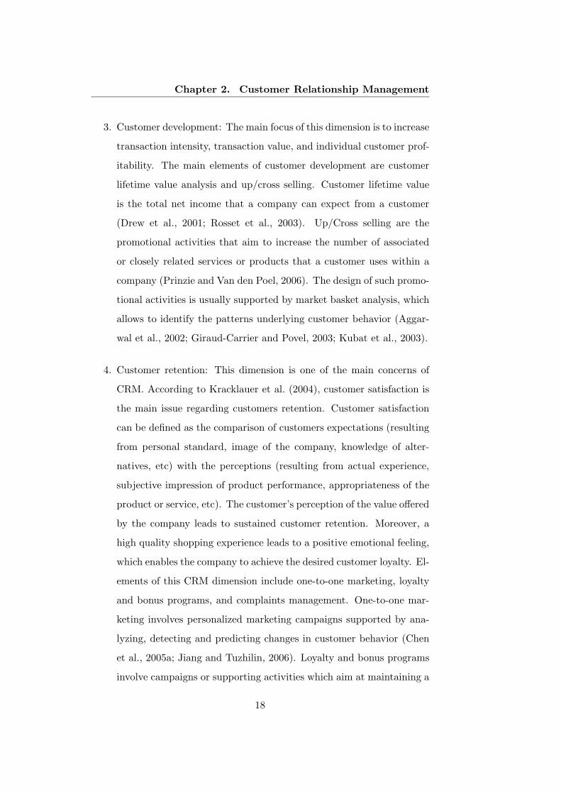
Figure 2.2, shows the dimensions of customer relationship management and
the tactical tools for achieving the respective core tasks. Some tools, such as
benchmarking and one-to-one marketing, are common to several dimensions.
Figure 2.2: CRM instruments. (Kracklauer et al., 2004)
2.4.2 Applications
Despite its apparent contribution for companies’ sustainability and growth,
analytical CRM has not been systematically applied. In fact, research on
analytical CRM is quite limited (Anderson et al., 2007).
Regarding the customer identification dimension, Han et al. (2012) seg-
mented customers of a telecom operator in China, by considering customer
value as a derivation from historic value, current value, long-term value,
19
Chapter 2. Customer Relationship Management
loyalty and credit. Kim et al. (2006) proposed a framework for analyzing
customer value and segmenting customers based on their value. This paper
used a wireless telecommunication company as case study. Bae et al. (2003)
proposed a web adverts selector for e-newspaper providers, which person-
alizes advertising messages. For this purpose, customers were splitted into
different segments, on the basis of their preferences and interests. Woo
et al. (2005) suggested a customer targeting method, based on a customer
visualization map, which depicts value distribution across customer needs
and customer characteristics. This customers’ map was applied to a Korean
credit card company. Chen et al. (2003) built a model for a tour company
that predicts in which tours a new customer will be interested. This model
uses information concerning customers profiles and information about the
tours they joined before.
Concerning customer attraction, Baesens et al. (2002) approached purchase
incidence modeling for a major European direct mail company. It evaluated
whether a customer would repurchase or not, considering different customer
profiling predictors. Buckinx et al. (2004) proposed a model that makes pre-
dictions concerning the redemption of coupons distributed by a fast-moving
consumer goods retailer. This model considers historical customer behavior
and customer demographics. Ahn et al. (2006) introduced an optimized al-
gorithm which classifies customers into either purchasing or non-purchasing
groups. To validate the algorithm proposed, this study used data from an
online diet portal site in Korea. This site contains all kind of services for
online diets, such as information providing, community services and a shop-
ping mall. The algorithm was also tested by using data from another online
shop. Kim and Street (2004) suggested a model that enables to identify op-
timal campaign targets, based on each individual’s likelihood of responding
to campaign messages positively. The model was tested in a recreational
vehicle insurance context, by using data from many European households.
20
2.4 Analytical CRM
Chiu (2002) proposed a model to identify the customers who are most likely
to buy life insurance products. This purchasing behavior model was devel-
oped using real cases provided by one worldwide insurance direct marketing
company.
Regarding customer development, Baesens et al. (2004) focused on predict-
ing whether a newly acquired customer would increase or decrease his/her
future spending, by considering initial purchase information. This research
was conducted on scanner data of a large Belgian do-it-yourself (DIY) retail
chain. Rosset et al. (2003) used analytical models for estimating the effect
of various marketing activities on customers lifetime value. This study was
developed in the telecommunications industry context. Brijs et al. (2004)
tackled the problem of product assortment analysis, and introduced a mi-
croeconomic integer-programming model for product selection, considering
the sets of products which are usually purchased together. The empirical
study was based on data from a fully-automated convenience store. Chen
et al. (2005b) introduced a method to discover customer purchasing pat-
terns from stores’ transactional databases, by identifying products which
were usually purchased together. Prinzie and Van den Poel (2006) analyzed
purchase sequences to identify cross-buying patterns what might be used to
discover cross-selling opportunities in the financial services context.
Customer retention has deserved particular attention in CRM literature.
Larivire and Van den Poel (2005) analyzed the impact of a broad set of
explanatory variables on churn probability. This set of variables included
past customer behavior, observed customer heterogeneity and some typical
variables related to intermediaries on three measures of customer outcome:
next buy, partial-defection and customers’ profitability evolution. This anal-
ysis used a large European financial services company as case study. Hung
et al. (2006) estimated churn prediction in mobile telecommunication by
using customer demographics, billing information, contract/service status,
21
Chapter 2. Customer Relationship Management
call detail records, and service change log. Chen et al. (2005a) integrated
customer behavioral variables, demographic variables, and a transactional
database to establish a method for identifying changes in customer behav-
ior. The approach was developed using data from a retail store. Ha et al.
(2006) proposed a content recommender system which suggests web con-
tent, in this case news articles. It considers users preferences observed when
he/she is vising an internet news site. The study developed by Cho et al.
(2005) proposed a new methodology for product recommendation that uses
customer purchase sequences. The methodology proposed was applied to
a large department store in Korea. Chang et al. (2006) used customers’
online navigation patterns to assist user’s search of items of interest. This
study conducted an empirical analysis designed for the case of an electronic
commerce store selling digital cameras.
2.5 Summary and conclusions
This chapter reviewed the evolution of the marketing concept. The history
of marketing can be divided into 4 distinct periods: the production, the
sales, the marketing, and the relationship periods. Relationship marketing
represents the current state of marketing. Customer relationship manage-
ment is part of relationship marketing. CRM is about establishing, cultivat-
ing, maintaining and optimizing long term mutually valuable relationships.
The benefits underlying companies’ adoption of CRM strategies are: lower
cost of acquiring customers, higher customer profitability, increased cus-
tomer retention and loyalty, reduced cost of sales, integration of the whole
organization, improved customer service and easy evaluation of customers
profitability.
CRM integrates mainly three components: operational, collaborative and
analytical. Operational CRM concerns the automation of processes in order
22
2.5 Summary and conclusions
to facilitate customers service; collaborative CRM focuses on the interaction
with customers and analytical CRM concerns the analysis of customer data,
for a broad range of business purposes. Focusing on analytical CRM, this in-
cludes four main dimensions: customer identification, customer attraction,
customer development and customer retention. From the analysis of the
literature it is fair to conclude that the study of each of these dimensions
in the retail sector is still incipient, enabling room for improvement. There-
fore, this thesis aims to address analytical CRM dimensions by proposing
innovator models, supported by data mining techniques, to reinforce the
relationship between companies and customers.
23

Chapter 2. Customer Relationship Management
24
Chapter 3
Introduction to datamining techniques
3.1 Introduction
Knowledge discovery in databases (KDD) is a CRM analytical tool which has
received considerable attention in recent years (Frawley et al., 1992). This
chapter provides a summary of the knowledge discovery process. Moreover,
since this research required the use of several data mining techniques, this
chapter also includes a summary of the main data mining techniques used
to assist analytical CRM.
This chapter is organized as follows. Section 3.2 introduces the process of
KDD. Section 3.3 defines data mining and introduces its main techniques.
It also shows the relationship between data mining and analytical customer
relationship management. The following sections describe the data mining
techniques mainly used to support analytical customer relationship manage-
ment (i.e. clustering - Section 3.4, classification - Section 3.5 and association
- Section 3.6). Section 3.7 summarizes and concludes.
25
Chapter 3. Introduction to data mining techniques
3.2 Knowledge discovery
The advance in IT over the last decades and the penetration of IT into orga-
nizations enabled the storage and analysis of a large volume of data, creating
a good opportunity to obtain knowledge. However, the transformation of
data into useful knowledge is a slow and difficult process.
The first applications of techniques to extract knowledge from databases
faced many difficulties, mainly due to the fact that existing algorithms had
been designed in laboratory, where, in general, the quality of the data was
guaranteed and the amount of data was very limited (Fogel and Fogel, 1995).
Therefore, it became evident the need of following a systematic process
focused on data preparation. This would allow increasing the confidence
in the results obtained. The systematic approach combining a data pre-
processing stage and a post-processing stage is called knowledge discovery
in databases (KDD) and it was first discussed at the first KDD workshop in
1989.
KDD is a complex process concerning the discovery of relationships and
other patterns in the data. It includes a well-defined set of stages, ranging
from data preparation to the extraction of information from the data. KDD
uses tools from different fields, such as statistics, artificial intelligence, data
visualization and patterns recognition. The techniques developed in these
areas of study are used in KDD to extract knowledge from the databases.
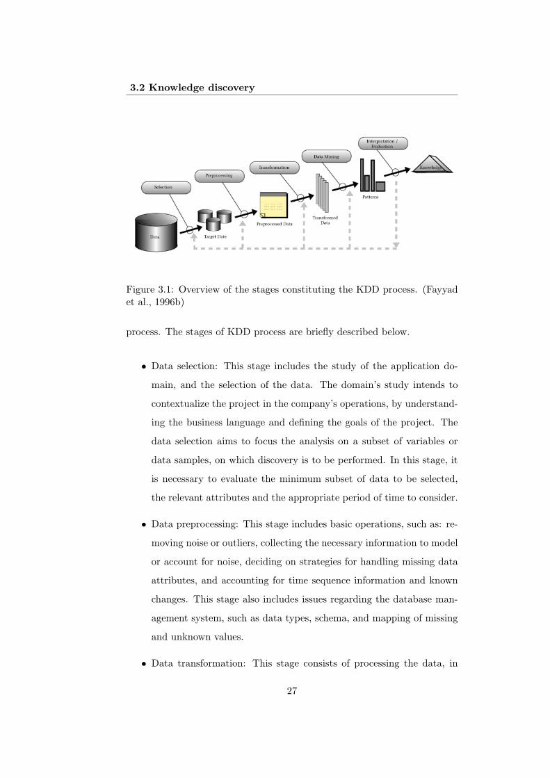
The KDD process is outlined in Figure 3.1. This process includes several
stages, consisting of data selection, data treatment, data pre-processing,
data mining and interpretation of the results. This process is interactive,
since there are many decisions that must be taken by the decision-maker
during the process. Moreover, this is an iterative process, since it allows to
go back to a previous stage and then proceed with the knowledge discovery
26
3.2 Knowledge discovery
Figure 3.1: Overview of the stages constituting the KDD process. (Fayyadet al., 1996b)
process. The stages of KDD process are briefly described below.
• Data selection: This stage includes the study of the application do-
main, and the selection of the data. The domain’s study intends to
contextualize the project in the company’s operations, by understand-
ing the business language and defining the goals of the project. The
data selection aims to focus the analysis on a subset of variables or
data samples, on which discovery is to be performed. In this stage, it
is necessary to evaluate the minimum subset of data to be selected,
the relevant attributes and the appropriate period of time to consider.
• Data preprocessing: This stage includes basic operations, such as: re-
moving noise or outliers, collecting the necessary information to model
or account for noise, deciding on strategies for handling missing data
attributes, and accounting for time sequence information and known
changes. This stage also includes issues regarding the database man-
agement system, such as data types, schema, and mapping of missing
and unknown values.
• Data transformation: This stage consists of processing the data, in
27
Chapter 3. Introduction to data mining techniques
order to convert the data in the appropriate formats for applying data
mining algorithms. The most common transformations are: data nor-
malization, data aggregation and data discretization. Some algorithms
require data normalization to be effectively implemented. To normal-
ize the data, each value is subtracted the mean and divided by the
standard deviation. Usually, data mining algorithms work on a single
data table and consequently it is necessary to aggregate the data from
different tables. Some algorithms only deal with quantitative or qual-
itative data. Therefore, it may be necessary to discretize the data, i.e.
map qualitative data to quantitative data, or map quantitative data
to qualitative data.
• Data mining: This stage consists of discovering patterns in a dataset
previously prepared. Several algorithms are evaluated in order to iden-
tify the most appropriate for a specific task. The selected one is then
applied to the relevant data, in order to find implicit relationships or
other interesting patterns.
• Interpretation/Evaluation: This stage consists of interpreting the dis-
covered patterns and evaluating their utility and importance with re-
spect to the application domain. In this stage it can be concluded that
some relevant attributes were ignored in the analysis, thus suggesting
the need to replicate the process with an updated set of attributes.
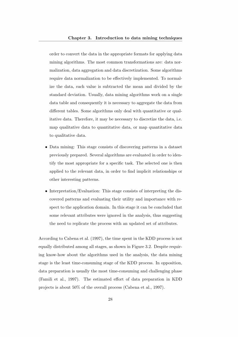
According to Cabena et al. (1997), the time spent in the KDD process is not
equally distributed among all stages, as shown in Figure 3.2. Despite requir-
ing know-how about the algorithms used in the analysis, the data mining
stage is the least time-consuming stage of the KDD process. In opposition,
data preparation is usually the most time-consuming and challenging phase
(Famili et al., 1997). The estimated effort of data preparation in KDD
projects is about 50% of the overall process (Cabena et al., 1997).
28
3.3 Data mining and analytical CRM
Figure 3.2: Typical effort needed for each stage of the KDD process (Cabenaet al., 1997).
3.3 Data mining and analytical CRM
Berry and Linoff (2000) defines data mining as the process of exploring
and analyzing huge datasets, in order to find patterns and rules which can
be important to solve a problem. Berson et al. (1999); Lejeune (2001);
Berry and Linoff (2004) define data mining as the process of extracting
or detecting hidden patterns or information from large databases. Data
mining is motivated by the need for techniques to support the decision maker
in analyzing, understanding and visualizing the huge amounts of data that
have been gathered from business and are stored in data warehouses or other
information repositories. Data mining is an interdisciplinary domain that
gets together artificial intelligence, database management, machine learning,
data visualization, mathematic algorithms, and statistics.
29
Chapter 3. Introduction to data mining techniques
Data mining is considered by some authors as the core stage of the KDD
process and consequently it has received by far the most attention in the
literature (Fayyad et al., 1996a). Data mining applications have emerged
from a variety of fields including marketing, banking, finance, manufacturing
and health care (Brachman et al., 1996). Moreover, data mining has also
been applied to other fields, such as spatial, telecommunications, web and
multimedia. According to the field and type of data available, the most
appropriate data mining technique can be different.
A wide variety of data mining techniques are described in the literature.
Thus, an overview of these techniques can often consist of long lists of seem-
ingly unrelated and highly specific techniques. Despite this, most data min-
ing techniques can be seen as compositions of a few basic techniques and
principles. Several can be applied for the execution of a specific task. The
performance of each one depends upon the task to be carried out and the
quality of the data available. According to Ngai et al. (2009), association,
classification, clustering, forecasting, regression, sequence discovery and vi-
sualization cover the main data mining techniques. These groups of data
mining techniques can be summarized as follows:
• Association intends to determine relationships between attributes in
databases (Mitra et al., 2002; Ahmed, 2004; Jiao et al., 2006). The fo-
cus is on deriving multi-attribute correlations, satisfying support and
confidence thresholds. Examples of association model outputs are as-
sociation rules. For example, these rules can be used to describe which
items are commonly purchased with other items in grocery stores.
• Classification aims to map a data item into one of several predefined
categorical classes (Berson et al., 1999; Mitra et al., 2002; Chen et al.,
2003; Ahmed, 2004). For example, a classification model can be used
to identify loan applicants as low, medium, or high credit risks.
30
3.3 Data mining and analytical CRM
• Clustering, similarly to classification models, aims to map a data item
into one of several categorical classes (or clusters). Unlike classification
in which the classes are predefined, in clustering the classes are deter-
mined from the data. Clusters are defined by finding natural groups of
data items, based on similarity metrics or probability density models
(Berry and Linoff, 2004; Mitra et al., 2002; Giraud-Carrier and Povel,
2003; Ahmed, 2004). For example, a clustering model can be used to
group customers who usually buy the same group of products.
• Forecasting estimates the future value of a certain attribute, based
on records’ patterns. It deals with outcomes measured as continuous
variables (Ahmed, 2004; Berry and Linoff, 2004). The central elements
of forecasting analytics are the predictors, i.e. the attributes measured
for each item in order to predict future behavior. Demand forecast is
a typical example of a forecasting model whose predictors could be for
example price and advertisement.
• Regression maps a data item to a real-value prediction variable (Mitra
et al., 2002; Giraud-Carrier and Povel, 2003). Curve fitting, mod-
eling of causal relationships, prediction (including forecasting) and
testing scientific hypotheses about relationships between variables are
frequent applications of regression.
• Sequence discovery intends to identify relationships among items over
time (Berson et al., 1999; Mitra et al., 2002; Giraud-Carrier and Povel,
2003). It can essentially be thought of as association discovery over a
temporal database. For example, sequence analysis can be developed
to determine, if customers had enrolled for plan A, then what is the
next plan that customer is likely to take-up and in what time-frame.
• Visualization is used to present the data such that users can notice
complex patterns (Shaw, 2001). Usually it is used jointly with other
31
Chapter 3. Introduction to data mining techniques
data mining models to provide a clearer understanding of the dis-
covered patterns or relationships (Turban et al., 2010). Examples of
visualization applications include the mindmaps.
Data mining techniques can also be categorized in supervised learning and
unsupervised learning. Supervised learning requires that the dataset con-
tains predefined targets that represent the classes of data items or the be-
haviors that are going to be predicted. For example, a supervised model can
be trained to identify patterns which enable to classify bank clients as poten-
tial loan defaulters or non-defaulters. Unsupervised learning techniques do
not require the dataset to contain the target variables (e.g. classes of data
items) (Bose and Chen, 2009). An unsupervised model can be trained to
group customers into similar unknown groups. Most data mining techniques
are supervised. The most common unsupervised techniques are those used
for clustering.
The use of data mining techniques to extract meaningful information from
data is very promising. In fact, many companies have collected and stored
data resulting from the interactions with customers, suppliers and business
partners. However, according to Berson et al. (1999), the inability to find
valuable information in the data has prevented companies from converting
these data into valuable and useful knowledge. Particularly within the ana-
lytical CRM dimension, data mining techniques are becoming popular ways
of analyzing customer data. In fact, the employment of data mining to
support CRM analytical dimension is seen as an emerging tendency (Ngai
et al., 2009). Data mining techniques can be used to support competitive
marketing strategies by analyzing and understanding customer behaviors
and characteristics, so as to acquire and maintain customers and maximize
customer value. The selection of appropriate data mining techniques which
can extract useful knowledge from large customer databases is of utmost
32
3.3 Data mining and analytical CRM
importance. According to Berson et al. (1999), when carefully selected,
the data mining techniques are one of the best supporting tools of CRM
decisions.
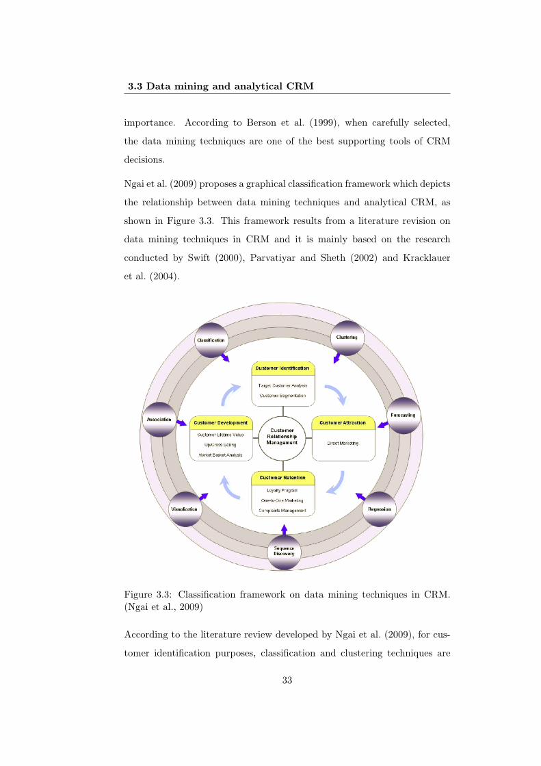
Ngai et al. (2009) proposes a graphical classification framework which depicts
the relationship between data mining techniques and analytical CRM, as
shown in Figure 3.3. This framework results from a literature revision on
data mining techniques in CRM and it is mainly based on the research
conducted by Swift (2000), Parvatiyar and Sheth (2002) and Kracklauer
et al. (2004).
Figure 3.3: Classification framework on data mining techniques in CRM.(Ngai et al., 2009)
According to the literature review developed by Ngai et al. (2009), for cus-
tomer identification purposes, classification and clustering techniques are
33
Chapter 3. Introduction to data mining techniques
the most often used. If the objective is to attract customers, classification
techniques are the most frequently used, while if the objective is to re-
tain customers, association and classification are the most frequently used.
Concerning customers’ development, association techniques are the most
frequent. Despite this, it is known that a combination of data mining tech-
niques is often required to support each CRM analytical dimension (Ngai
et al., 2009).
Since the research reported in this thesis focuses on customers identification,
attraction, development and retention, this involved a study of clustering,
classification and association data mining techniques. This study aimed
at exploring the techniques and getting insight into the advantages and
disadvantages of each one, in order to develop models that could meet the
objectives of the company. The next sections explore more deeply clustering,
classification and association data mining techniques.
3.4 Clustering
Clustering techniques are very useful to gain knowledge from a dataset.
Clustering analyzes data items without considering a known class label. In
general, the class labels are not present in the training data, since they are
not known. Therefore, clustering can be used to generate such labels. The
items are clustered according to the principle of intraclass similarity maxi-
mization and the interclass similarity minimization. It means that clusters
are formed so that items within a cluster have high similarity, but are very
dissimilar to items in other clusters. Each cluster that is formed can be seen
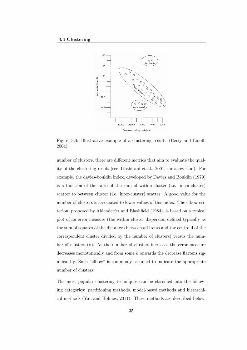
as a class of items, from which rules can be derived. Figure 3.4 illustrates
an example of clustered items.
In most clustering algorithms, the number of clusters is set as a user param-
eter (Thilagamani and Shanthi, 2010). In order to support the choice of the
34
3.4 Clustering
Figure 3.4: Illustrative example of a clustering result. (Berry and Linoff,2004)
number of clusters, there are different metrics that aim to evaluate the qual-
ity of the clustering result (see Tibshirani et al., 2001, for a revision). For
example, the davies-bouldin index, developed by Davies and Bouldin (1979)
is a function of the ratio of the sum of within-cluster (i.e. intra-cluster)
scatter to between cluster (i.e. inter-cluster) scatter. A good value for the
number of clusters is associated to lower values of this index. The elbow cri-
terion, proposed by Aldenderfer and Blashfield (1984), is based on a typical
plot of an error measure (the within cluster dispersion defined typically as
the sum of squares of the distances between all items and the centroid of the
correspondent cluster divided by the number of clusters) versus the num-
ber of clusters (k). As the number of clusters increases the error measure
decreases monotonically and from some k onwards the decrease flattens sig-
nificantly. Such “elbow” is commonly assumed to indicate the appropriate
number of clusters.
The most popular clustering techniques can be classified into the follow-
ing categories: partitioning methods, model-based methods and hierarchi-
cal methods (Yau and Holmes, 2011). These methods are described below.
35
Chapter 3. Introduction to data mining techniques
Variable clustering is also explored below. Although the usual aim of the
framework of clustering is to cluster items, variable clustering is also rele-
vant.
3.4.1 Partitioning methods
Partitioning methods (or non-hierarchical methods) create clusters by opti-
mizing an objective partitioning criterion, such as the distance dissimilarity
function. Given a database of n items, a partitioning method constructs k
partitions of the data, where each partition represents a cluster and k ≤ n.
Each group must contain at least one item and each item must belong to
exactly one group. Please note that this second requirement can be relaxed
in some fuzzy partitioning techniques (see Kaufman and Rousseeuw, 1990,
for further details).
The most popular and commonly used partitioning methods are k -means
and k -medoids (Witten et al., 2001; Huang et al., 2007).
k-means
The k -means algorithm, introduced by Forgy (1965) and later developed by
MacQueen (1967), assigns a set of n items to k clusters. The number of clus-
ters is pre-defined by the analyst. According to the partitioning algorithms
definition, k -means aims at achieving a high intracluster similarity and a
low intercluster similarity. Therefore, each item is assigned to the closest
cluster, based on the minimum distance between the item and the cluster
mean. This algorithm requires the definition of the initial seeds (initial items
defined as the clusters mean) in the first iteration of the algorithm. After
classifying a new item, it is calculated a new mean for the corresponding
cluster and the process continues. This algorithm involves several iterations
which differ concerning the initial seeds. The process is finished when the
36
3.4 Clustering
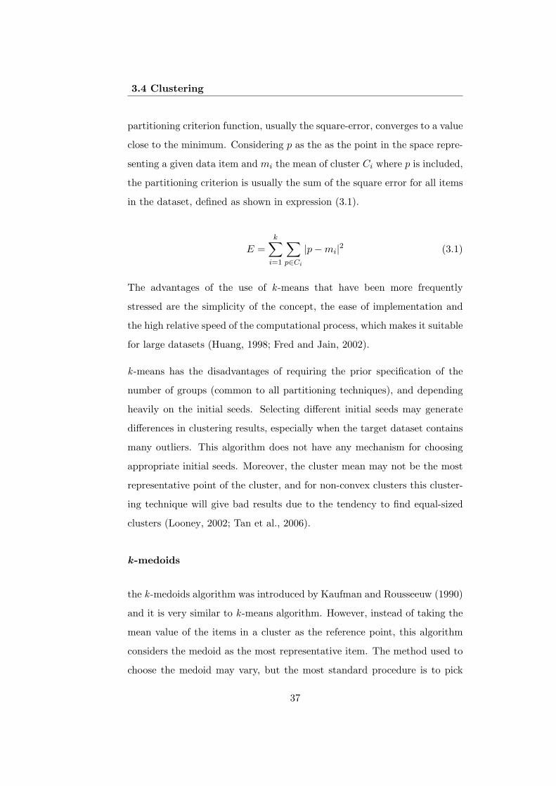
partitioning criterion function, usually the square-error, converges to a value
close to the minimum. Considering p as the as the point in the space repre-
senting a given data item and mi the mean of cluster Ci where p is included,
the partitioning criterion is usually the sum of the square error for all items
in the dataset, defined as shown in expression (3.1).
E =k∑
i=1
∑p∈Ci
|p−mi|2 (3.1)
The advantages of the use of k -means that have been more frequently
stressed are the simplicity of the concept, the ease of implementation and
the high relative speed of the computational process, which makes it suitable
for large datasets (Huang, 1998; Fred and Jain, 2002).
k -means has the disadvantages of requiring the prior specification of the
number of groups (common to all partitioning techniques), and depending
heavily on the initial seeds. Selecting different initial seeds may generate
differences in clustering results, especially when the target dataset contains
many outliers. This algorithm does not have any mechanism for choosing
appropriate initial seeds. Moreover, the cluster mean may not be the most
representative point of the cluster, and for non-convex clusters this cluster-
ing technique will give bad results due to the tendency to find equal-sized
clusters (Looney, 2002; Tan et al., 2006).
k-medoids
the k -medoids algorithm was introduced by Kaufman and Rousseeuw (1990)
and it is very similar to k -means algorithm. However, instead of taking the
mean value of the items in a cluster as the reference point, this algorithm
considers the medoid as the most representative item. The method used to
choose the medoid may vary, but the most standard procedure is to pick
37
Chapter 3. Introduction to data mining techniques
the item which has the lowest average distance to all other items. Since this
is an operation computationally demanding, sometimes the search for the
medoid is made only on a sample of items.
The advantage of k -medoids over k -means is that k -medoids is less sensitive
to noise or extreme values. However, due to the medoid selection procedure,
this is a time-consuming algorithm (Hutchison et al., 2005b).
3.4.2 Model-based methods
Model-based methods attempt to optimize the fit between the dataset and a
specific mathematical model. Such methods are often based on the assump-
tion that the data are generated by a mixture of probability distributions,
in which each single probability distribution represents a different cluster
(Han and Kamber, 2006). The clustering problem consists of estimating
the parameters of the probability distributions, so as to best fit the data.
Consequently, a particular clustering method can be expected to work well
when the data conform to the model.
The advantages and disadvantages of model-based methods depend on the
specific model. The most prominent model-based method is the expectation-
maximization algorithm. Self-organizing maps, included in neural networks
approaches, and cobweb, included in conceptual clustering approaches are
also well-known model-based methods.
Expectation-maximization
The expectation-maximization (EM) algorithm, introduced by Dempster
et al. (1977), is an extension of the k -means partitioning algorithm and
aims at finding the parameter estimates of the probability distributions
which maximize the likelihood function. Instead of assigning each item
to a dedicated cluster, EM assigns each item to a cluster according to a
38
3.4 Clustering
weight representing the probability of membership. It means that there are
no strict boundaries between clusters.
The EM algorithm takes into consideration that each training item belongs
to an unknown distribution. Therefore, it adopts the procedure used for k -
means clustering algorithm, selecting k items to represent the cluster. The
EM algorithm also starts with an initial guess for the parameters of the
models for each cluster and uses them to calculate the cluster probabilities
for each item. Then, it iteratively uses these probabilities to adjust the
parameters. The first step, the calculation of cluster probabilities (which
are the “expected” class values) is called “expectation”; the second, the
calculation of the distribution parameters is called “maximization” of the
likelihood of the distributions given the data (Witten et al., 2001).
The expectation step consists of calculating the probability of cluster mem-
bership of item xi for each cluster Ck using expression (3.2) and the corre-
sponding assignment of the items to the clusters.
P (xi ∈ Ck) = p(Ck|xi) =p(Ck)p(xi|Ck)
p(xi)(3.2)
p(xi|Ck) follows the normal (i.e., Gaussian) distribution around mean µk,
and covariance∑
k.
The maximization step uses the probability estimated to re-estimate the
model parameters, in order to maximize the likelihood of the distributions
given the data. The new mean can be defined using expression (3.3), where
n is the number of items.
µk =
∑n1 xiP (xi ∈ Ck)∑n1 P (xi ∈ Ck)
(3.3)
The new covariance is obtained from expression (3.4):
39
Chapter 3. Introduction to data mining techniques
∑k
=
∑n1 P (xi ∈ Ck)(xi − µk)(xi − µk)
T∑n1 P (xi ∈ Ck)
(3.4)
In case of Gaussian distributions, mean and covariance are sufficient statis-
tics.
EM is a semantically strong algorithm, as it not only provides clusters, but
also produces complex models for the clusters which can also capture cor-
relation and dependence among the attributes. However, the use of this
algorithm has an essential drawback: it requires the definition of the appro-
priate data models to optimize, which can be difficult for many real datasets.
Actually, in some cases the assumption of Gaussian distributions is rather
strong. Moreover, using EM there is no guarantee of convergence to a global
optimum, so multiple runs may produce different results.
Self-organizing maps
Self-organizing maps (SOMs) (Kohonen, 1982), sometimes called kohonen
maps, is a popular neural network method for clustering. Artificial neu-
ral networks (ANN), proposed by Mcculloch and Pitts (1943), is a method
derived from the models of neurophysiology. It consists of processing infor-
mation, inspired by the human brain. The neural networks are formed by a
set of elements called neurons which are organized into structures more or
less complex (lattice). Each neuron is a processing unit that receives stim-
ulus (data) and learns to recognize patterns in the data. As in the brain,
the neurons are interconnected by branches through which the stimulus are
propagated.
SOMs enable to project a high-dimensional input space on a low-dimensional
space (usually 2-D or 3-D) such that the distance and proximity relationship
(i.e., topology) is preserved as much as possible. A SOM is composed by
40
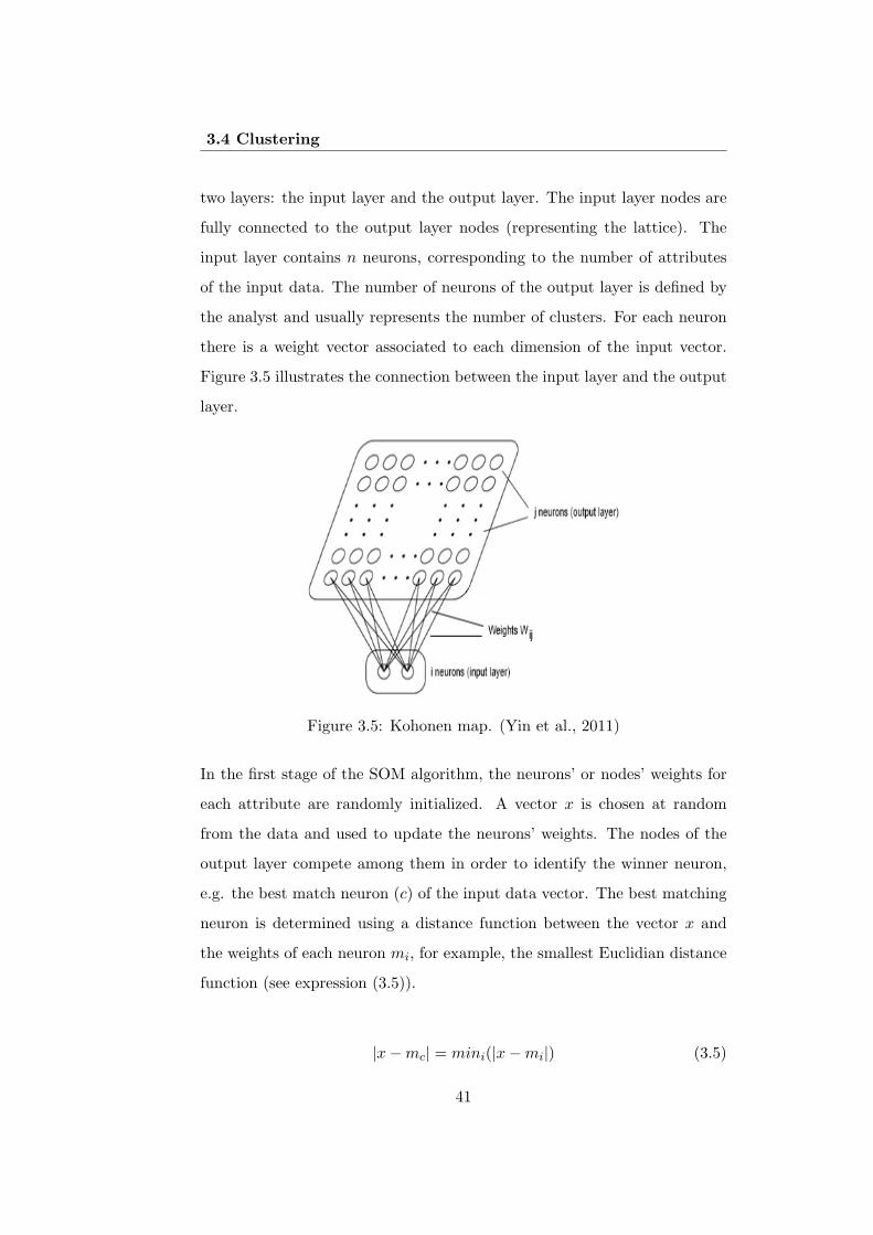
3.4 Clustering
two layers: the input layer and the output layer. The input layer nodes are
fully connected to the output layer nodes (representing the lattice). The
input layer contains n neurons, corresponding to the number of attributes
of the input data. The number of neurons of the output layer is defined by
the analyst and usually represents the number of clusters. For each neuron
there is a weight vector associated to each dimension of the input vector.
Figure 3.5 illustrates the connection between the input layer and the output
layer.
Figure 3.5: Kohonen map. (Yin et al., 2011)
In the first stage of the SOM algorithm, the neurons’ or nodes’ weights for
each attribute are randomly initialized. A vector x is chosen at random
from the data and used to update the neurons’ weights. The nodes of the
output layer compete among them in order to identify the winner neuron,
e.g. the best match neuron (c) of the input data vector. The best matching
neuron is determined using a distance function between the vector x and
the weights of each neuron mi, for example, the smallest Euclidian distance
function (see expression (3.5)).
|x−mc| = mini(|x−mi|) (3.5)
41
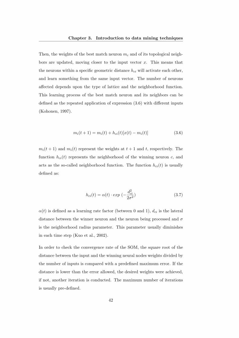
Chapter 3. Introduction to data mining techniques
Then, the weights of the best match neuron mc and of its topological neigh-
bors are updated, moving closer to the input vector x. This means that
the neurons within a specific geometric distance hci will activate each other,
and learn something from the same input vector. The number of neurons
affected depends upon the type of lattice and the neighborhood function.
This learning process of the best match neuron and its neighbors can be
defined as the repeated application of expression (3.6) with different inputs
(Kohonen, 1997).
mi(t+ 1) = mi(t) + hci(t)[x(t)−mi(t)] (3.6)
mi(t+ 1) and mi(t) represent the weights at t+ 1 and t, respectively. The
function hci(t) represents the neighborhood of the winning neuron c, and
acts as the so-called neighborhood function. The function hci(t) is usually
defined as:
hci(t) = α(t) · exp (− d2ci2σ2
) (3.7)
α(t) is defined as a learning rate factor (between 0 and 1), dci is the lateral
distance between the winner neuron and the neuron being processed and σ
is the neighborhood radius parameter. This parameter usually diminishes
in each time step (Kuo et al., 2002).
In order to check the convergence rate of the SOM, the square root of the
distance between the input and the winning neural nodes weights divided by
the number of inputs is compared with a predefined maximum error. If the
distance is lower than the error allowed, the desired weights were achieved,
if not, another iteration is conducted. The maximum number of iterations
is usually pre-defined.
42
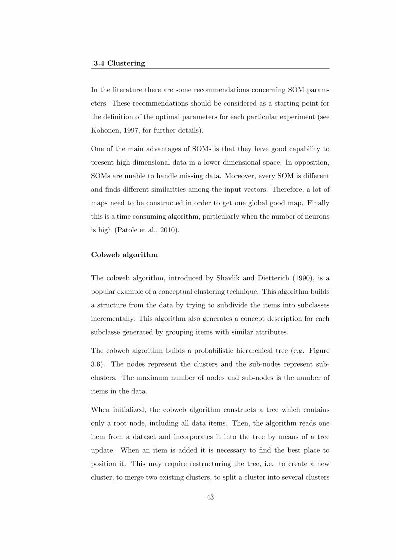
3.4 Clustering
In the literature there are some recommendations concerning SOM param-
eters. These recommendations should be considered as a starting point for
the definition of the optimal parameters for each particular experiment (see
Kohonen, 1997, for further details).
One of the main advantages of SOMs is that they have good capability to
present high-dimensional data in a lower dimensional space. In opposition,
SOMs are unable to handle missing data. Moreover, every SOM is different
and finds different similarities among the input vectors. Therefore, a lot of
maps need to be constructed in order to get one global good map. Finally
this is a time consuming algorithm, particularly when the number of neurons
is high (Patole et al., 2010).
Cobweb algorithm
The cobweb algorithm, introduced by Shavlik and Dietterich (1990), is a
popular example of a conceptual clustering technique. This algorithm builds
a structure from the data by trying to subdivide the items into subclasses
incrementally. This algorithm also generates a concept description for each
subclasse generated by grouping items with similar attributes.
The cobweb algorithm builds a probabilistic hierarchical tree (e.g. Figure
3.6). The nodes represent the clusters and the sub-nodes represent sub-
clusters. The maximum number of nodes and sub-nodes is the number of
items in the data.
When initialized, the cobweb algorithm constructs a tree which contains
only a root node, including all data items. Then, the algorithm reads one
item from a dataset and incorporates it into the tree by means of a tree
update. When an item is added it is necessary to find the best place to
position it. This may require restructuring the tree, i.e. to create a new
cluster, to merge two existing clusters, to split a cluster into several clusters
43
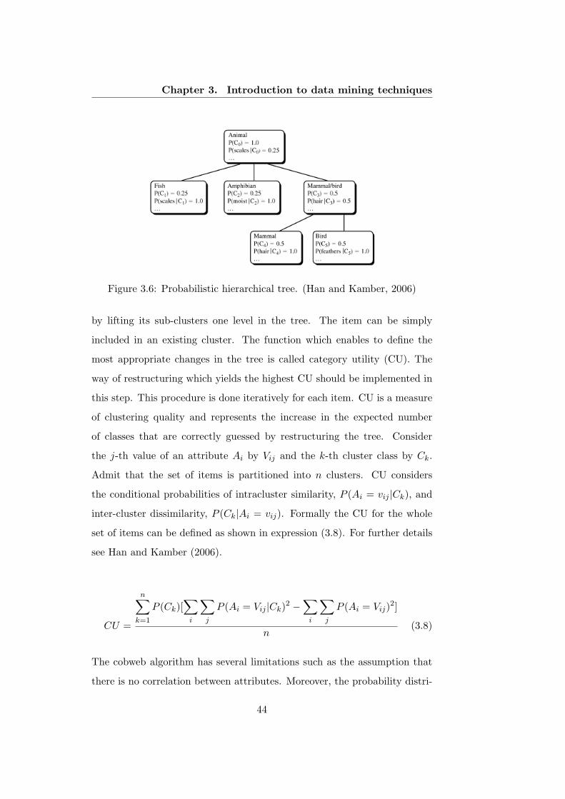
Chapter 3. Introduction to data mining techniques
Figure 3.6: Probabilistic hierarchical tree. (Han and Kamber, 2006)
by lifting its sub-clusters one level in the tree. The item can be simply
included in an existing cluster. The function which enables to define the
most appropriate changes in the tree is called category utility (CU). The
way of restructuring which yields the highest CU should be implemented in
this step. This procedure is done iteratively for each item. CU is a measure
of clustering quality and represents the increase in the expected number
of classes that are correctly guessed by restructuring the tree. Consider
the j-th value of an attribute Ai by Vij and the k-th cluster class by Ck.
Admit that the set of items is partitioned into n clusters. CU considers
the conditional probabilities of intracluster similarity, P (Ai = vij |Ck), and
inter-cluster dissimilarity, P (Ck|Ai = vij). Formally the CU for the whole
set of items can be defined as shown in expression (3.8). For further details
see Han and Kamber (2006).
CU =
n∑k=1
P (Ck)[∑i
∑j
P (Ai = Vij |Ck)2 −
∑i
∑j
P (Ai = Vij)2]
n(3.8)
The cobweb algorithm has several limitations such as the assumption that
there is no correlation between attributes. Moreover, the probability distri-
44
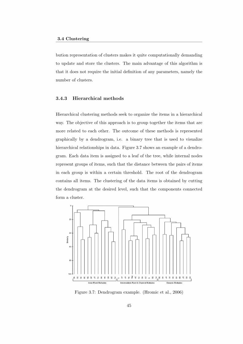
3.4 Clustering
bution representation of clusters makes it quite computationally demanding
to update and store the clusters. The main advantage of this algorithm is
that it does not require the initial definition of any parameters, namely the
number of clusters.
3.4.3 Hierarchical methods
Hierarchical clustering methods seek to organize the items in a hierarchical
way. The objective of this approach is to group together the items that are
more related to each other. The outcome of these methods is represented
graphically by a dendrogram, i.e. a binary tree that is used to visualize
hierarchical relationships in data. Figure 3.7 shows an example of a dendro-
gram. Each data item is assigned to a leaf of the tree, while internal nodes
represent groups of items, such that the distance between the pairs of items
in each group is within a certain threshold. The root of the dendrogram
contains all items. The clustering of the data items is obtained by cutting
the dendrogram at the desired level, such that the components connected
form a cluster.
Figure 3.7: Dendrogram example. (Hromic et al., 2006)
45
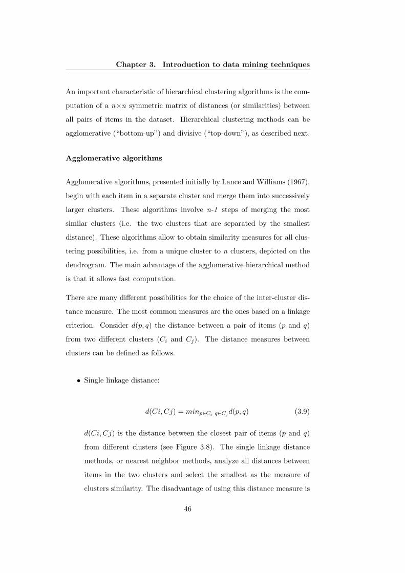
Chapter 3. Introduction to data mining techniques
An important characteristic of hierarchical clustering algorithms is the com-
putation of a n×n symmetric matrix of distances (or similarities) between
all pairs of items in the dataset. Hierarchical clustering methods can be
agglomerative (“bottom-up”) and divisive (“top-down”), as described next.
Agglomerative algorithms
Agglomerative algorithms, presented initially by Lance and Williams (1967),
begin with each item in a separate cluster and merge them into successively
larger clusters. These algorithms involve n-1 steps of merging the most
similar clusters (i.e. the two clusters that are separated by the smallest
distance). These algorithms allow to obtain similarity measures for all clus-
tering possibilities, i.e. from a unique cluster to n clusters, depicted on the
dendrogram. The main advantage of the agglomerative hierarchical method
is that it allows fast computation.
There are many different possibilities for the choice of the inter-cluster dis-
tance measure. The most common measures are the ones based on a linkage
criterion. Consider d(p, q) the distance between a pair of items (p and q)
from two different clusters (Ci and Cj). The distance measures between
clusters can be defined as follows.
• Single linkage distance:
d(Ci,Cj) = minp∈Ci q∈Cjd(p, q) (3.9)
d(Ci,Cj) is the distance between the closest pair of items (p and q)
from different clusters (see Figure 3.8). The single linkage distance
methods, or nearest neighbor methods, analyze all distances between
items in the two clusters and select the smallest as the measure of
clusters similarity. The disadvantage of using this distance measure is
46
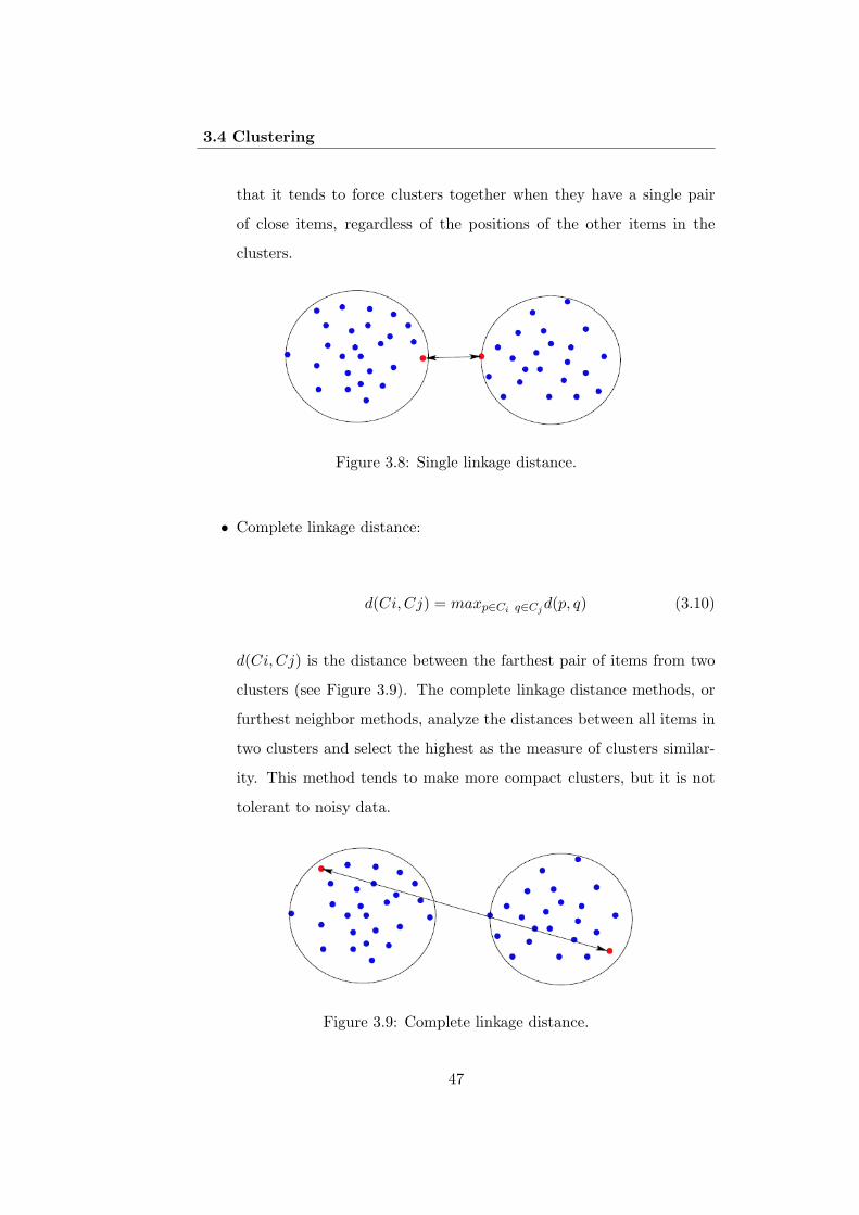
3.4 Clustering
that it tends to force clusters together when they have a single pair
of close items, regardless of the positions of the other items in the
clusters.
Figure 3.8: Single linkage distance.
• Complete linkage distance:
d(Ci,Cj) = maxp∈Ci q∈Cjd(p, q) (3.10)
d(Ci,Cj) is the distance between the farthest pair of items from two
clusters (see Figure 3.9). The complete linkage distance methods, or
furthest neighbor methods, analyze the distances between all items in
two clusters and select the highest as the measure of clusters similar-
ity. This method tends to make more compact clusters, but it is not
tolerant to noisy data.
Figure 3.9: Complete linkage distance.
47
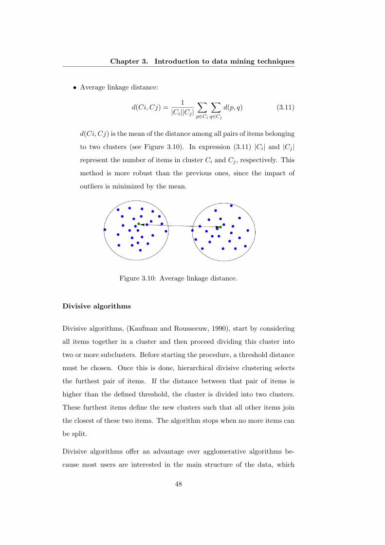
Chapter 3. Introduction to data mining techniques
• Average linkage distance:
d(Ci,Cj) =1
|Ci||Cj |∑p∈Ci
∑q∈Cj
d(p, q) (3.11)
d(Ci,Cj) is the mean of the distance among all pairs of items belonging
to two clusters (see Figure 3.10). In expression (3.11) |Ci| and |Cj |
represent the number of items in cluster Ci and Cj , respectively. This
method is more robust than the previous ones, since the impact of
outliers is minimized by the mean.
Figure 3.10: Average linkage distance.
Divisive algorithms
Divisive algorithms, (Kaufman and Rousseeuw, 1990), start by considering
all items together in a cluster and then proceed dividing this cluster into
two or more subclusters. Before starting the procedure, a threshold distance
must be chosen. Once this is done, hierarchical divisive clustering selects
the furthest pair of items. If the distance between that pair of items is
higher than the defined threshold, the cluster is divided into two clusters.
These furthest items define the new clusters such that all other items join
the closest of these two items. The algorithm stops when no more items can
be split.
Divisive algorithms offer an advantage over agglomerative algorithms be-
cause most users are interested in the main structure of the data, which
48
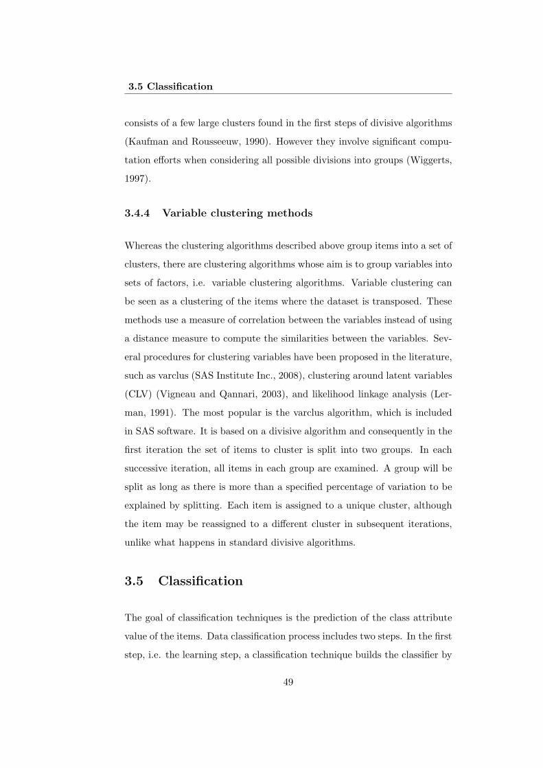
3.5 Classification
consists of a few large clusters found in the first steps of divisive algorithms
(Kaufman and Rousseeuw, 1990). However they involve significant compu-
tation efforts when considering all possible divisions into groups (Wiggerts,
1997).
3.4.4 Variable clustering methods
Whereas the clustering algorithms described above group items into a set of
clusters, there are clustering algorithms whose aim is to group variables into
sets of factors, i.e. variable clustering algorithms. Variable clustering can
be seen as a clustering of the items where the dataset is transposed. These
methods use a measure of correlation between the variables instead of using
a distance measure to compute the similarities between the variables. Sev-
eral procedures for clustering variables have been proposed in the literature,
such as varclus (SAS Institute Inc., 2008), clustering around latent variables
(CLV) (Vigneau and Qannari, 2003), and likelihood linkage analysis (Ler-
man, 1991). The most popular is the varclus algorithm, which is included
in SAS software. It is based on a divisive algorithm and consequently in the
first iteration the set of items to cluster is split into two groups. In each
successive iteration, all items in each group are examined. A group will be
split as long as there is more than a specified percentage of variation to be
explained by splitting. Each item is assigned to a unique cluster, although
the item may be reassigned to a different cluster in subsequent iterations,
unlike what happens in standard divisive algorithms.
3.5 Classification
The goal of classification techniques is the prediction of the class attribute
value of the items. Data classification process includes two steps. In the first
step, i.e. the learning step, a classification technique builds the classifier by
49
Chapter 3. Introduction to data mining techniques
analyzing a training dataset including the attribute vector and the class
value. Because the class value of each training itemset is provided, this
step is also known as supervised learning. In the second step, the learning
function obtained previously is used to predict the attribute class label of
the target dataset.
There are many classification techniques in the literature (Zhang et al.,
2007). The next sections present some of the most used: logistic regression,
decision trees, random forests and artificial neural networks.
3.5.1 Logistic regression
Logistic regression is a classical statistical technique used for classification.
There are several regression techniques that differ in terms of research ob-
jectives and variable characteristics. Linear regression is the regression tech-
nique most frequently used. It considers continuous dependent variables and
assumes that the relationship between the dependent variable and the inde-
pendent variables (or attributes) is linear. When the objective is to examine
the effect of a single independent variable on a dependent variable, a simple
regression can be used. When the objective is to examine the effect of mul-
tiple independent variables on a dependent variable, a multiple regression
can be used.
Logistic regression is a particular case of linear models. This regression
technique considers binary dependent variables, instead of continuous vari-
ables, and assumes a linear relationship between the dependent variable
expressed in the logit scale, i.e. using a log-odds transformation, and the
independent variables. In the logit regression, the dependent variable is the
probability that an event will occur, hence it is constrained between 0 and 1.
Ordinary linear regression techniques are inappropriate to estimate the de-
pendent variable, because they enable the dependent variable to fall outside
50
3.5 Classification
the 0 − 1 range. Assume x as a column vector of independent variables and
π = P (Y = 1|x) as the probability that the event Y occurs. The logistic
regression takes the form shown in expression (3.12):
lnπ
1− π= α+ βTx (3.12)
α is the intercept parameter and βT contains the independent variables
coefficients (Hosmer and Lemeshow, 2000).
The main reasons behind the application of logistic regression are the ease
of use and the quick and robust results obtained (Buckinx and Van den
Poel, 2005). Moreover, logistic regression does not rely on assumptions
of normality for the independent variables or the errors and may handle
non-linear effects (Fahrmeir, 1985). The main concerns of the application
of logistic regression are: the difficulty in detecting complex relationships
between input and output variables, unless stated by the modeler, and the
difficulty in detecting implicit interactions among the independent variables
(Ayer et al., 2010).
3.5.2 Decision trees
Decision tree classifiers are a well-known technique of classification which
allows to easily obtain the classification rules. A decision tree has a tree
structure, where each node is either a leaf, which indicates the value of the
target attribute (class), or a decision node, which specifies some test to be
carried out on a single attribute value. Each outgoing branch represents an
outcome of the test (see Figure 3.11 for illustration purposes). A decision
tree can be used to predict the value of the class for all items, by starting at
the root of the tree and moving through it until a leaf node, which provides
the classification value.
51
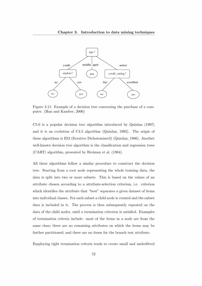
Chapter 3. Introduction to data mining techniques
Figure 3.11: Example of a decision tree concerning the purchase of a com-puter. (Han and Kamber, 2006)
C5.0 is a popular decision tree algorithm introduced by Quinlan (1997)
and it is an evolution of C4.5 algorithm (Quinlan, 1992). The origin of
these algorithms is ID3 (Iterative Dichotomiser3) (Quinlan, 1986). Another
well-known decision tree algorithm is the classification and regression trees
(CART) algorithm, presented by Breiman et al. (1984).
All these algorithms follow a similar procedure to construct the decision
tree. Starting from a root node representing the whole training data, the
data is split into two or more subsets. This is based on the values of an
attribute chosen according to a attribute-selection criterion, i.e. criterion
which identifies the attribute that “best” separates a given dataset of items
into individual classes. For each subset a child node is created and the subset
data is included in it. The process is then subsequently repeated on the
data of the child nodes, until a termination criterion is satisfied. Examples
of termination criteria include: most of the items in a node are from the
same class; there are no remaining attributes on which the items may be
further partitioned; and there are no items for the branch test attribute.
Employing tight termination criteria tends to create small and underfitted
52
3.5 Classification
decision trees. On the other hand, using loose stopping criteria tends to
generate large decision trees, which reflects anomalies in the training data
due to noise or outliers. Pruning methods originally suggested by Breiman
et al. (1984) were introduced to manage this trade-off.
Usually trees are built by considering a loose termination criterion, which
allows the decision tree to over-fit the data, i.e. the tree is too specialized on
the training set that it performs poorly on unseen data. Then, the over-fitted
tree is cut back into a smaller tree by removing the least relevant branches.
The main motivation for pruning is the increase of the generalization ability,
mainly in noisy domains (Bohanec and Bratko, 1994).
According to Friedl and Brodley (1997), the advantages of the decision trees
include the ability to handle data measured on different scales, the lack of
any assumptions concerning the frequency distributions of the data in each
classe, the flexibility, and the ability to handle non-linear relationships be-
tween attributes and classes. Moreover, decision trees are fast and easy to
train (Teeuwsen et al., 2004). They can also be used for attribute selec-
tion/reduction (Borak and Strahler, 1999). Finally, the analyst can easily
interpret a decision tree. One of the main drawbacks of the decision trees
is the instability, which means that different training datasets from a given
problem domain will produce very different trees (Breiman, 1996). In ad-
dition, decision trees may suffer from overfitting, conducting to suboptimal
performances (Dudoit et al., 2002).
The decision tree algorithms differ mainly in the termination criteria, men-
tioned above, in the attribute-selection criteria and in the pruning strategies.
The most popular attribute-selection criteria are: information gain, gain ra-
tio and gini index. These criteria are described below. The standard meth-
ods of pruning are: cost complexity, pessimistic pruning and reduced error
pruning algorithm (Esposito et al., 1997; Mingers, 1989; Quinlan, 1987).
53
Chapter 3. Introduction to data mining techniques
These methods are also described below.
Information gain
The information gain is a criterion that uses the entropy (with origin in the
information theory) as the impurity measure of the classification (Quinlan,
1987). If the impurity or randomness of a dataset with respect to the class
attribute is high, then the entropy is high. Admit that it is intended to par-
tition the dataset D on the attribute A, having v distinct values, and admit
that attribute A can be used to split D into v partitions {D1, D2, ..., Dv}.
The information gain for attribute A can be expressed by means of expres-
sion (3.13).
Information Gain(A) = Info(D)− InfoA(D) (3.13)
Info(D) is the expected information needed to classify an item in D and it
is given by expression (3.14).
Info(D) = −k∑
i=1
pilog2(pi) (3.14)
pi is the probability of an arbitrary item in D belonging to class Ci (for
i = 1, ..., k), and k is the number of distinct classes.
InfoA(D) is the expected information needed to classify an item from D
based on the partitioning by A and it is given by expression (3.15).
InfoA(D) =v∑
j=1
|Dj ||D|
× Info(Dj) (3.15)
The attribute A with the highest information gain is chosen as the splitting
attribute at each node.
54
3.5 Classification
Consider that instead of a discrete attribute, A is a continuous-valued at-
tribute. In this case, it is necessary to define the “best” split-point for A.
Therefore, the values of A are sorted in ascending order and typically the
midpoint between each pair of adjacent values is considered as a possible
split-point. Consequently, for each potential split-point, expression (3.15) is
computed. The point that enables to obtain the highest information gain
determines a subset D1 and a subset D2 satisfying A 6 split point and
A > split point, respectively.
Gain ratio
The gain ratio is a kind of normalization of the information gain. It is
defined as follows (Quinlan, 1992):
Gain Ratio(A) =Information Gain(A)
Split Info(A)(3.16)
Split Info(A) is given by expression (3.17).
Split Info(A) = −v∑
j=1
|Dj ||D|
× log2(|Dj ||D|
) (3.17)
Note that the gain ratio is not computed when the denominator is zero.
Moreover, the gain ratio may favor attributes for which the denominator is
very small.
In order to overcome these weaknesses, the selection of the splitting attribute
is usually done in two stages. First, the information gain is calculated for
all attributes. Then, for those attributes that have performed at least as
good as the average information gain, the gain ratio is computed and it is
selected the attribute that allows to obtain the highest gain ratio.
55
Chapter 3. Introduction to data mining techniques
Gini index
The gini index, introduced by Breiman et al. (1984), is a criterion that
measures the statistical dispersion of the target attribute value or class.
The gini index can be defined as shown in expression (3.19):
Gini(D) = 1−k∑
i=1
p2i (3.18)
pi is the probability of an item in D belongs to a class i. Admit again that it
is intended to partition the dataset D on the attribute A, having v distinct
values, and admit that attribute A can be used to split D into v partitions
{D1, D2, ..., Dv}. The gini index of the resulting partition is:
GiniA(D) =|D1||D|
Gini(D1) + ...+|Dv||D|
Gini(Dv) (3.19)
The attribute that minimizes the gini index is selected as the splitting at-
tribute. For continues-valued attributes, each possible split-point must be
considered, and the procedure is similar to that described for information
gain.
Cost complexity
One of the pruning algorithms is the cost complexity pruning algorithm. It
estimates a measure that combines the complexity of the pruned tree, i.e.,
a function of the number of leaves in the tree, and the error rate of the
tree, i.e., the percentage of items misclassified by the pruned tree. The cost-
complexity measure of the pruned tree takes the form shown in expression
(3.20):
56

3.5 Classification
α =ε(pruned(T, t), S)− ε(T, S)
|leaves(T )| − |leaves(pruned(T, t))|(3.20)
ε(T, S) represents the error rate of the tree T over the sample S and |leaves(T )|
represents the number of leaves in T . pruned(T, t) represents the tree when
the node t in T is replaced by a leaf (Maimon and Rokach, 2005). The
pruned tree which allows to minimize the cost-complexity measure defines
the resulting sub-tree.
Pessimistic pruning
The basic idea underlying pessimistic pruning is that the error ratio used in
cost complexity estimation is not reliable enough. Instead, a more realistic
measure (ε′(T, S)), known as continuity correction for binomial distribution,
given by expression (3.22) (Maimon and Rokach, 2005) is introduced.
ε′(T, S) = ε(T, S) +|leaves(T )|
2 · |S|(3.21)
Quinlan (1992) considers that the correction introduced still produces an
optimistic error rate and suggests pruning an internal node t if its error
rate is within one standard error of the minimum error tree (see expression
(3.22)).
ε′(pruned(T, t), S) ≤ ε′(T, S) +
√ε′(T, S) · (1− ε′(T, S))
|S|(3.22)
Reduced error pruning
This algorithm traverses over the internal nodes from the bottom to the
top, and checks for each internal node whether replacing it with the most
frequent class does not reduce the tree accuracy on a different dataset, i.e.
57
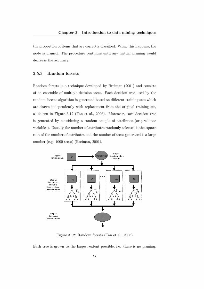
Chapter 3. Introduction to data mining techniques
the proportion of items that are correctly classified. When this happens, the
node is pruned. The procedure continues until any further pruning would
decrease the accuracy.
3.5.3 Random forests
Random forests is a technique developed by Breiman (2001) and consists
of an ensemble of multiple decision trees. Each decision tree used by the
random forests algorithm is generated based on different training sets which
are drawn independently with replacement from the original training set,
as shown in Figure 3.12 (Tan et al., 2006). Moreover, each decision tree
is generated by considering a random sample of attributes (or predictor
variables). Usually the number of attributes randomly selected is the square
root of the number of attributes and the number of trees generated is a large
number (e.g. 1000 trees) (Breiman, 2001).
Figure 3.12: Random forests.(Tan et al., 2006)
Each tree is grown to the largest extent possible, i.e. there is no pruning.
58
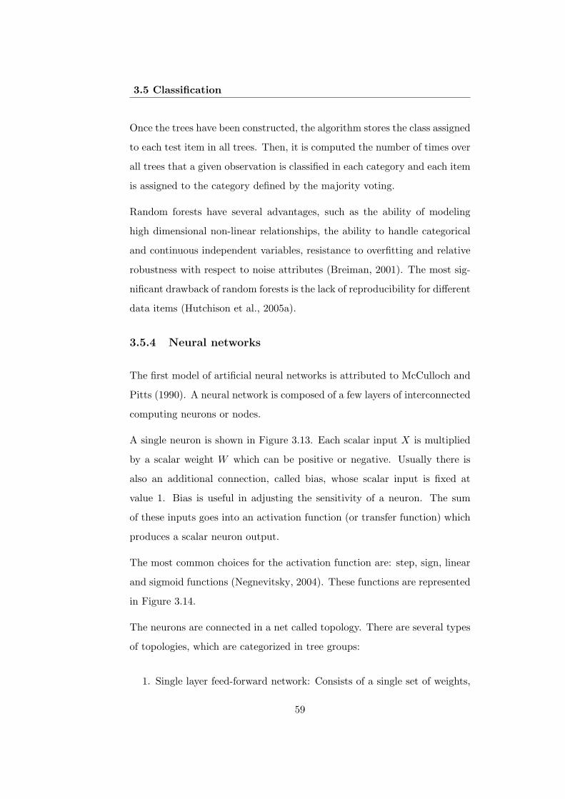
3.5 Classification
Once the trees have been constructed, the algorithm stores the class assigned
to each test item in all trees. Then, it is computed the number of times over
all trees that a given observation is classified in each category and each item
is assigned to the category defined by the majority voting.
Random forests have several advantages, such as the ability of modeling
high dimensional non-linear relationships, the ability to handle categorical
and continuous independent variables, resistance to overfitting and relative
robustness with respect to noise attributes (Breiman, 2001). The most sig-
nificant drawback of random forests is the lack of reproducibility for different
data items (Hutchison et al., 2005a).
3.5.4 Neural networks
The first model of artificial neural networks is attributed to McCulloch and
Pitts (1990). A neural network is composed of a few layers of interconnected
computing neurons or nodes.
A single neuron is shown in Figure 3.13. Each scalar input X is multiplied
by a scalar weight W which can be positive or negative. Usually there is
also an additional connection, called bias, whose scalar input is fixed at
value 1. Bias is useful in adjusting the sensitivity of a neuron. The sum
of these inputs goes into an activation function (or transfer function) which
produces a scalar neuron output.
The most common choices for the activation function are: step, sign, linear
and sigmoid functions (Negnevitsky, 2004). These functions are represented
in Figure 3.14.
The neurons are connected in a net called topology. There are several types
of topologies, which are categorized in tree groups:
1. Single layer feed-forward network: Consists of a single set of weights,
59
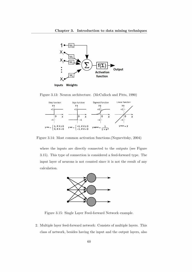
Chapter 3. Introduction to data mining techniques
Figure 3.13: Neuron architecture. (McCulloch and Pitts, 1990)
Figure 3.14: Most common activation functions.(Negnevitsky, 2004)
where the inputs are directly connected to the outputs (see Figure
3.15). This type of connection is considered a feed-forward type. The
input layer of neurons is not counted since it is not the result of any
calculation.
Figure 3.15: Single Layer Feed-forward Network example.
2. Multiple layer feed-forward network: Consists of multiple layers. This
class of network, besides having the input and the output layers, also
60
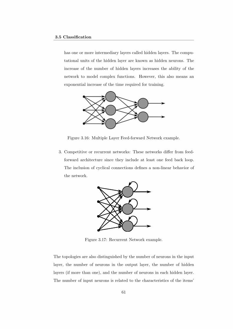
3.5 Classification
has one or more intermediary layers called hidden layers. The compu-
tational units of the hidden layer are known as hidden neurons. The
increase of the number of hidden layers increases the ability of the
network to model complex functions. However, this also means an
exponential increase of the time required for training.
Figure 3.16: Multiple Layer Feed-forward Network example.
3. Competitive or recurrent networks: These networks differ from feed-
forward architecture since they include at least one feed back loop.
The inclusion of cyclical connections defines a non-linear behavior of
the network.
Figure 3.17: Recurrent Network example.
The topologies are also distinguished by the number of neurons in the input
layer, the number of neurons in the output layer, the number of hidden
layers (if more than one), and the number of neurons in each hidden layer.
The number of input neurons is related to the characteristics of the items’
61
Chapter 3. Introduction to data mining techniques
attributes. Discrete-valued attributes may be encoded such that there is
one input neuron per domain value. Continuous input attributes are usually
encoded by a unique neuron. Regarding the number of output neurons, one
neuron may be used to represent two classes (the value 1 represents one
class, and the value 0 represents the other class). If there are more than
two classes, then one output neuron per class is required. There are no
strict rules concerning the appropriate number of hidden layers and hidden
neurons. Network design is a trial-and-error process and may affect the
accuracy of the resulting trained network. Once a network has been trained
and its accuracy is not considered acceptable, it is common to repeat the
training process with a different network topology or a different set of initial
weights (Han and Kamber, 2006).
Before starting the network training process, the weights of the connections
are selected. These values are usually small and are randomly generated (e.g.
ranging from -1.0 to 1.0). Then, the network learning process is initialized,
by iteratively selecting an item from the training dataset. The network’s
prediction for each item is compared with the known value. For each training
item, the weights are modified so as to minimize the error (Errj) between
the network’s prediction and the known value. Expression (3.23) gives the
error in a neuron j, where Oj is the current output of neuron j, Tj is the
known target value, f ′ is the derivative of the activation function f and
inj is the sum of the weighted input coming into node j. The weights are
updated following expression (3.24). η is the learning rate parameter, a
constant typically ranging between 0.0 and 1.0. The learning rate is used to
avoid getting stuck at a local minimum in the decision space (i.e. where the
weights appear to converge, but is not the global optimum) and encourages
finding the global minimum.
Errj = f ′(inj)(Tj −Oj) (3.23)
62
3.6 Association
wij = wij + ηErrjOi (3.24)
These modifications are made in the “backwards” direction, i.e. from the
output layer, through each hidden layer down to the first hidden layer. An
iteration is finished when all items are considered. The process is finished
when the weights converge. In the process described, the weights are up-
dated after the presentation of each item. There is also an alternative ap-
proach in which the weights are updated after all items in the training set
have been presented (see Han and Kamber (2006) for further details).
Globally, neural network advantages have been more frequently reported
than disadvantages (Vellido et al., 1999). The main advantages pointed out
are the ability to accommodate large sample sizes, the suitability to han-
dle incomplete, missing or noisy data, the absence of assumptions about
the distribution of the data (since it is a non-parametric method) and the
ability to map any complex non-linearity and/or approximate any continu-
ous function. The main disadvantages of applying neural networks methods
are the difficulty of interpretation, thus being called “black-boxes”, and the
possibility of overfitting. Moreover, there is no formal rules to optimize the
neural network architecture, as well as the learning algorithm. Therefore,
different set up parameters can lead to different results. In addition, it is
required a long time to train the network.
3.6 Association
Association rule mining is a data mining application to extract patterns. As-
sociation rules are able to reveal interesting relationships in large databases.
A well-known example of an association rule application is the discovery
of patterns in retail sales data, namely products that are often purchased
63
Chapter 3. Introduction to data mining techniques
together. This is the standard application for association techniques and is
called market-basket analysis (Agrawal et al., 1993).
LetD be a database consisting of one table over n attributes {A1, A2, ..., An}
(e.g. products). Consider that each attribute Ai is nominal. In many real
world applications (such as the retail sales data) the attributes are binary
(e.g. presence or absence of one product in a particular market basket).
Let d be a record (e.g. a transaction) of the database D. d contains a
set of products X ⊆ {A1, A2, ..., An} if X ⊆ d. An association rule is an
implication X ⇒ Y where X,Y ⊆ {A1, A2, ..., An}, Y = ø and X ∪ Y = ø.
The support s(X) of a product set X is the proportion of records in D which
contain X. Therefore the support of an association rule, i.e. s(X ⇒ Y ),
is the proportion of records that contain both the antecedent X and the
consequent Y (see expression (3.25)). The confidence of the association
rule, i.e. c(X ⇒ Y ), is the proportion of records that contain X and that
contain Y (see expression (3.26)).
s(X ⇒ Y ) = P (X ∪ Y ) (3.25)
c(X ⇒ Y ) = P (Y |X) =s(X ∪ Y )
s(X)(3.26)
Another measure that characterizes an association rule is the lift. This
measure evaluates the level of dependency between the elements of an as-
sociation rule. It is obtained by dividing the support of X and Y , s(X,Y ),
representing the percentage of occurrences of X and Y in the same database,
by the product of the support of X and Y considered separately, as shown
in expression (3.27).
lift(X,Y ) = s(X,Y )/(s(X).s(Y )) (3.27)
64
3.6 Association
The lift represents the tendency to buy the product sets X and Y together.
If the lift is equal to 1, there is independence between the occurrence of sales
of product sets X and Y . If the lift is greater than 1, the products tend to be
bought together, and if it is lower than 1, they tend to be bought separately.
Rules presenting a lift less or equal than 1 are usually disregarded.
The algorithms used to discover the association rules in a database can be
generally divided in two steps: the frequent product sets discovering process
and the association rule generating process. The first step consists of select-
ing the product sets that have support higher than the minimum defined.
This is a time-consuming process (Erickson, 2009) and is usually developed
by using the apriori algorithm (Agrawal and Srikant, 1994) or the frequent-
pattern growth algorithm (Lan et al., 2009), that will be summarized below.
The second steps consists of using the frequent product sets identified in the
previous step to generate the rules. For every nonempty subset K of the fre-
quent product set L, K ⇒ (L−K) is an association rule if s(L)s(K) ≽ minconf ,
where minconf is the minimum confidence threshold.
3.6.1 Apriori algorithm
The apriori algorithm is an algorithm used to discover frequent products set.
The first step of the algorithm consists of calculating the support of each
individual product and selecting those that have a support higher than the
minimum defined, i.e. sets of frequent items of size 1, i.e. L1. A subsequent
step k, consists of two phases. First, the frequent product sets Lk−1 found
in the (k − 1)th step are used to generate the candidate sets Ck, by joining
the different Lk−1 sets. According to the Apriori property, any set Lk−1
that is not frequent cannot be part of a frequent k-set, and consequently it
is not part of Ck. For example, to find C3 it is necessary to look at pairs in
L2 that have one item in common, e.g. (a1, a2) and (a1, a3), and combine
them, e.g. (a1, a2, a3). Second, the database is scanned and the support of
65
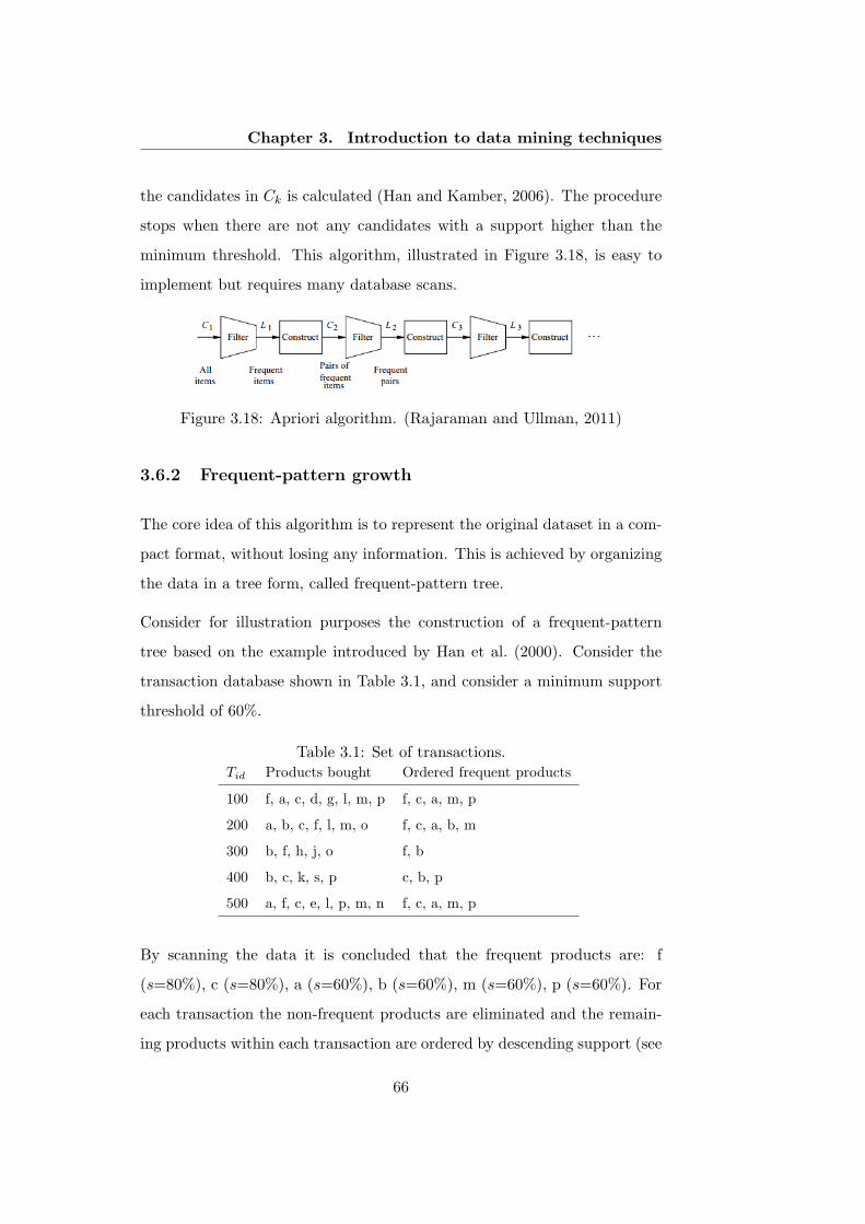
Chapter 3. Introduction to data mining techniques
the candidates in Ck is calculated (Han and Kamber, 2006). The procedure
stops when there are not any candidates with a support higher than the
minimum threshold. This algorithm, illustrated in Figure 3.18, is easy to
implement but requires many database scans.
Figure 3.18: Apriori algorithm. (Rajaraman and Ullman, 2011)
3.6.2 Frequent-pattern growth
The core idea of this algorithm is to represent the original dataset in a com-
pact format, without losing any information. This is achieved by organizing
the data in a tree form, called frequent-pattern tree.
Consider for illustration purposes the construction of a frequent-pattern
tree based on the example introduced by Han et al. (2000). Consider the
transaction database shown in Table 3.1, and consider a minimum support
threshold of 60%.
Table 3.1: Set of transactions.Tid Products bought Ordered frequent products
100 f, a, c, d, g, l, m, p f, c, a, m, p
200 a, b, c, f, l, m, o f, c, a, b, m
300 b, f, h, j, o f, b
400 b, c, k, s, p c, b, p
500 a, f, c, e, l, p, m, n f, c, a, m, p
By scanning the data it is concluded that the frequent products are: f
(s=80%), c (s=80%), a (s=60%), b (s=60%), m (s=60%), p (s=60%). For
each transaction the non-frequent products are eliminated and the remain-
ing products within each transaction are ordered by descending support (see
66
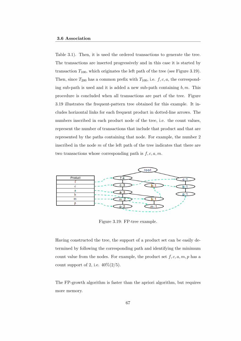
3.6 Association
Table 3.1). Then, it is used the ordered transactions to generate the tree.
The transactions are inserted progressively and in this case it is started by
transaction T100, which originates the left path of the tree (see Figure 3.19).
Then, since T200 has a common prefix with T100, i.e. f, c, a, the correspond-
ing sub-path is used and it is added a new sub-path containing b,m. This
procedure is concluded when all transactions are part of the tree. Figure
3.19 illustrates the frequent-pattern tree obtained for this example. It in-
cludes horizontal links for each frequent product in dotted-line arrows. The
numbers inscribed in each product node of the tree, i.e. the count values,
represent the number of transactions that include that product and that are
represented by the paths containing that node. For example, the number 2
inscribed in the node m of the left path of the tree indicates that there are
two transactions whose corresponding path is f, c, a,m.
Figure 3.19: FP-tree example.
Having constructed the tree, the support of a product set can be easily de-
termined by following the corresponding path and identifying the minimum
count value from the nodes. For example, the product set f, c, a,m, p has a
count support of 2, i.e. 40%(2/5).
The FP-growth algorithm is faster than the apriori algorithm, but requires
more memory.
67
Chapter 3. Introduction to data mining techniques
3.7 Conclusion
This chapter presented the process of KDD, which includes data selection,
data preprocessing, data transformation, data mining and interpretation or
evaluation. Focusing on the data mining stage, it explored the techniques
more frequently used to support customer relationship management, i.e.
clustering, association and classification techniques.
Clustering techniques are used to predict targets that represent non-predefined
classes of data items. These techniques are appropriate to segment cus-
tomers and consequently can support the model presented in Chapter 5.
Moreover, these techniques may be used to group customers’ shopping bas-
kets, as done in the model presented in Chapter 6.
Association techniques are used to detect relationships between attributes.
These techniques can be used in business applications such as market basket
analysis to find associations between sets of products. Thus, association
techniques may support the design of differentiated marketing actions in
Chapter 5.
Classification techniques are used to predict targets that represent prede-
fined classes of data items. Therefore, these techniques can be used to
predict whether or not a customer is going to leave the company, such as
done in Chapter 7 and Chapter 8.
There are many data mining techniques in the literature. Clustering tech-
niques include mainly partitioning algorithms, (e.g. k -means and k -medoids),
model-based algorithms, (e.g. expectation-maximization algorithm, self or-
ganizing maps and cobweb algorithm), and hierarchical algorithms, (e.g.
agglomerative and divisive algorithms). Classification techniques include lo-
gistic regression, decision trees, random forests and neural networks. Asso-
ciation techniques include apriori algorithm and frequent-pattern algorithm.
68

3.7 Conclusion
All techniques presented in this chapter have some advantages and disad-
vantages. Indeed, there is no consensus on the techniques that should be
used to analyze data from a specific setting. Usually there are no a pri-
ori guarantees of success and reliability. Particularly, when handling large
datasets, analysts often select the techniques according to their processing
speed. This is also the criterion that guided the selection of the algorithms
to assist the models developed in this doctoral work. The motivation for the
use of each specific technique is mentioned in each chapter.
69

Chapter 3. Introduction to data mining techniques
70
Chapter 4
Case study: description ofthe retail company
4.1 Introduction
This chapter presents the retail chain used as case study. Section 4.2 de-
scribes the company’s position in the market, the existing store formats,
the classification of the products and the organizational structure. Section
4.3 presents the loyalty program of the company and gives emphasis to the
segmentation methods and promotional policies. Section 4.4 characterizes
the company’s customers, mainly in terms of value spent and frequency of
visits. Finally, Section 4.5 presents the conclusions.
4.2 Company’s description
The company used as case study is one of the largest food retailers in Europe.
This company is a reference in the retail market, having started a revolution
in the consumption habits and commercial patterns in the country where it
is based, with the implementation of the first hypermarket in the 80s.
The company’s strategy consists of consolidating its leadership position in
71
Chapter 4. Case study: description of the retail company
the market where it is based and expanding the frontiers of business, taking
advantage of resources and skills development. These goals derive from the
company vision of leadership in the business. The company is expecting to
take advantage of the synergies drawn from the current portfolio of stores,
the reinforcement of the value-for-money offer, the implementation of the
best management practices and consequent operational efficiency increase,
the development of management and human resources, the incentives for
pro-active innovation, and the permanent focus on customers.
This company has a chain of foodbased stores, i.e. hypermarkets, large
supermarkets and small supermarkets. These formats differ essentially by
the range and price of products offered and by the sales area. Moreover,
the company has other stores specialized in different business units, such as
deep frozen products, garden and domestic pets, health, well-being and eye
care. The company’s stores are spread across different countries in Europe.
The company owns about 400 stores in the geographical area considered in
this study, corresponding to a sales area of about 544.000 m2.
Foodbased stores sell products which are categorized in 5 departments: gro-
cery, perishables, light bazaar, heavy bazaar and textile. The grocery de-
partment includes non-perishable food, such as grocery and drinks. This
department also includes hygiene and cleaning products. The perishables
department contains products from the butchery, fishery, bakery, fruits and
vegetables. The light bazaar department includes products for decoration,
culture (e.g. books and DVDs) and house. The heavy bazaar department
includes electric appliances, photographic material, video, computer hard-
ware and televisions. The textile department includes clothes, shoes and
accessories. Besides classifying its products by departments, the company
also classifies its products in other levels, such as business unit, category
and subcategory. The company characterizes its foodbased store products in
about 30 business units (e.g. Grocery, Baby textile), in about 150 categories
72
4.3 Loyalty program
(e.g. Milk/Soy drinks, Baby underwear) and in about 570 subcategories (e.g.
Pasteurized milk, Baby pijama).
The company’s hypermarkets are stores of large dimension, usually with
areas between 8000 and 12000 m2. Hypermarkets sell products from gro-
cery, perishables, light bazaar, heavy bazaar and textile departments. These
stores provide very competitive prices and are located in the main urban
centres, usually close to the main shopping centres. Large supermarkets
are stores with a shopping area of about 2000 m2. These stores also sell
products from grocery, perishables, light bazaar, heavy bazaar and textile
departments, at a competitive price. They are located close to small urban
centres. Small supermarkets are convenience stores, with an average dimen-
sion of 800 m2. These stores sell products from grocery, perishables and
light bazaar departments. These stores are directed to clients who value
proximity, convenience and high service quality, for which they are willing
to pay higher prices. These stores are concentrated in metropolitan areas, in
residential neighborhoods or in areas of high traffic. It is important to note
that, apart from the area of products’ exposition, all stores have warehouses,
products’ reception areas, customers’ support areas and point-of-sale (POS)
areas.
4.3 Loyalty program
In the last decades, it was observed an increase in the competition in high-
scale retail business. In this context, the company felt the need to redefine
its strategy, to achieve high sales performance in the stores. This was mainly
done by intensifying marketing actions.
In 2007 the company launched its loyalty card that can be used in all stores.
The card allows customers to take full advantage of continuous promotional
campaigns and to accumulate discounts valid for 12 months following the
73
Chapter 4. Case study: description of the retail company
purchase. Currently, the loyalty card database contains about 9 million
accounts, i.e. 3 million cardholders plus 6 million associated or family cards.
Approximately 85% of the total number of transactions are done using the
loyalty card.
The loyalty program enabled collecting data on each customer profile, i.e.
customer name, address, date of birth, gender, number of people in the
household, the telephone number and the number of one identification doc-
ument. This data is collected when customers join the loyalty program by
filling out a form. The use of the loyalty card by customers has also enabled
collecting data regarding customers’ transactions, i.e. date, time, store,
products and prices.
The data stored in the company databases allows segmenting the customers
in two ways. One of the segmentation models currently used by the com-
pany consists of grouping customers based on their shopping habits. This
segmentation model is a simplified version of the “recency, frequency and
monetary” (RFM) model, and is called internally: “frequency and mone-
tary value” (FM) model. According to the values of these two variables, the
company specifies 8 groups of customers. Each client is assigned to one of
these groups, according to the average number of purchases done and the
average amount of money spent per purchase. The changes in the percent-
age of customers belonging to each group are used to guide the marketing
actions required to meet the company’s objectives. For example, if the num-
ber of customers in the clusters with more visits to the store decreases, the
company is alerted to launch marketing campaigns in order to motivate cus-
tomers to go to the stores more often. The other method of segmentation is
based on customer necessities and preferences. In this case, customers are
grouped in 7 segments according to the mix of categories of products they
purchase. Each segment is defined by using a clustering algorithm in which
customers that purchase similar percentages of products from predefined
74
4.4 Customers characterization
groups of products are grouped. This segmentation method is still under
development and has only been used to conduct some pilot experiments of
customized promotions.
There are four main types of promotional actions, currently implemented
by the company:
• 5e to spend in future visits to the store per each 500e spent on pur-
chases recorded through the loyalty card.
• Discounts on specific products advertised in the store shelves and
leaflets, that are applicable to all customers with a loyalty card.
• Discounts on purchases done on selected days (percentual discount or
a pre-defined value of discount on the total amount spent on a given
purchase). These are applicable to customers that present at POS the
discount coupon sent by mail.
• Discounts for specific products on selected days. These can be sent by
mail or issued at POS.
The first three types of promotions do not differentiate between customers of
different segments. Currently, the target of the fourth type of promotional
actions is defined by a model based on the historical purchases of the prod-
uct included in the promotion. The discounts are only issued to the most
frequent buyers of the product, or to those customers who do not normally
buy the product, to encourage new buyers.
4.4 Customers characterization
The information collected through the loyalty card enables the company
to characterize its customers. In order to support the development of the
75
Chapter 4. Case study: description of the retail company
doctoral research, the company made available two distinct databases. Each
database included transactional data on the client identity number, the date
and time of the transaction, the product transacted and the price of the
product. In addition to the transactions information, each database included
some demographic information for each customer: residence postcode, city,
date of birth, gender, number of persons in the household. The first database
provided (Database 1) included the records of the 2.202.267 customers who
shopped in the company stores in October and November 2009. This was
the basis of the studies reported in Chapter 5 and Chapter 6. The second
database provided by the company (Database 2) included the records of the
581.002 customers who shopped in two hypermarkets between January 2009
and December 2010. This was the basis of the studies reported in Chapter
7 and Chapter 8.
The preparation of Database 1 involved the following procedure. Customers
whose average amount of money spent per purchase or the average number
of purchases per month was out of the range of the mean plus three standard
deviations were excluded. Since it was intended to focus the study only on
customers who are final consumers it was also decided to remove from the
database all customers whose average amount of money spent per purchase
was greater than 500e. These represented 0.75% of the customers included
in the original database. Usually purchases exceeding this value are done
by small retailers that resell the products in competing stores. After this
selection process, the database contained 2.142.439 customers.
The preparation of Database 2 involved the selection of new customers. New
customers were considered to be those who made no purchase in the first
half of 2009 but spent at least 100e until the end of 2010. This corresponded
to a total of 95.147 new customers.
The following analysis of customers characteristics is based on Database
76
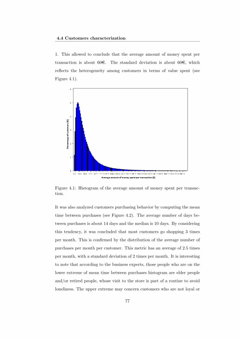
4.4 Customers characterization
1. This allowed to conclude that the average amount of money spent per
transaction is about 60e. The standard deviation is about 60e, which
reflects the heterogeneity among customers in terms of value spent (see
Figure 4.1).
Figure 4.1: Histogram of the average amount of money spent per transac-tion.
It was also analyzed customers purchasing behavior by computing the mean
time between purchases (see Figure 4.2). The average number of days be-
tween purchases is about 14 days and the median is 10 days. By considering
this tendency, it was concluded that most customers go shopping 3 times
per month. This is confirmed by the distribution of the average number of
purchases per month per customer. This metric has an average of 2.5 times
per month, with a standard deviation of 2 times per month. It is interesting
to note that according to the business experts, those people who are on the
lower extreme of mean time between purchases histogram are elder people
and/or retired people, whose visit to the store is part of a routine to avoid
loneliness. The upper extreme may concern customers who are not loyal or
77
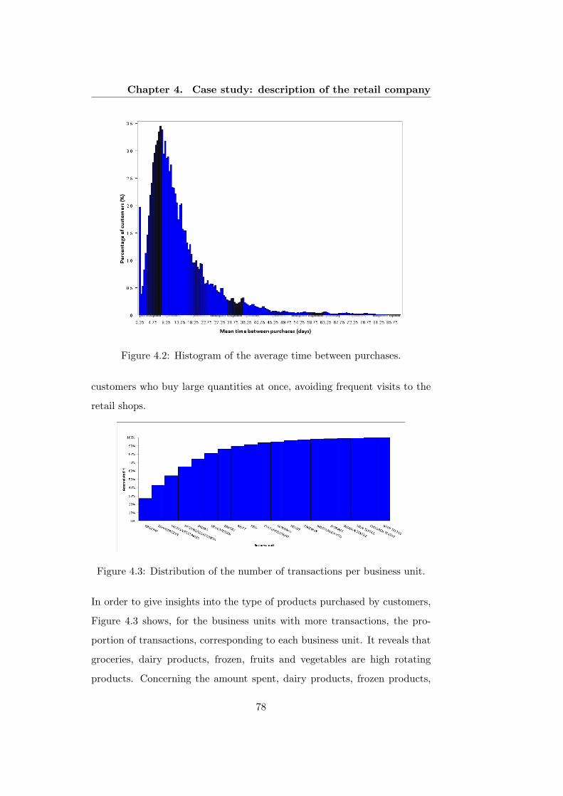
Chapter 4. Case study: description of the retail company
Figure 4.2: Histogram of the average time between purchases.
customers who buy large quantities at once, avoiding frequent visits to the
retail shops.
Figure 4.3: Distribution of the number of transactions per business unit.
In order to give insights into the type of products purchased by customers,
Figure 4.3 shows, for the business units with more transactions, the pro-
portion of transactions, corresponding to each business unit. It reveals that
groceries, dairy products, frozen, fruits and vegetables are high rotating
products. Concerning the amount spent, dairy products, frozen products,
78
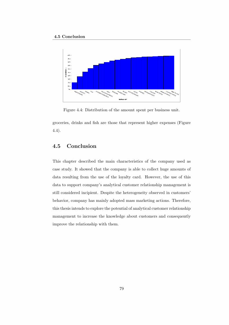
4.5 Conclusion
Figure 4.4: Distribution of the amount spent per business unit.
groceries, drinks and fish are those that represent higher expenses (Figure
4.4).
4.5 Conclusion
This chapter described the main characteristics of the company used as
case study. It showed that the company is able to collect huge amounts of
data resulting from the use of the loyalty card. However, the use of this
data to support company’s analytical customer relationship management is
still considered incipient. Despite the heterogeneity observed in customers’
behavior, company has mainly adopted mass marketing actions. Therefore,
this thesis intends to explore the potential of analytical customer relationship
management to increase the knowledge about customers and consequently
improve the relationship with them.
79

Chapter 4. Case study: description of the retail company
80
Chapter 5
Behavioral marketsegmentation to supportdifferentiated promotionsdesign
5.1 Introduction
Customers segmentation followed by the design of differentiated promotions
allows companies to efficiently target their customers. This chapter proposes
a model to segment customers according to their behavior, reflected by the
frequency and monetary value of the purchases. This chapter also proposes
a model that enables the identification of product associations within seg-
ments, which can base the definition of products more appropriate to include
in differentiated promotions.
The structure of the remainder of this chapter is as follows. Section 5.2
contextualizes the study concerning segmentation and market basket anal-
ysis (MBA) methods available in the literature. Section 5.3 presents the
methodology. Section 5.4 discusses the results and Section 5.5 highlights
the conclusions.
81
Chapter 5. Behavioral market segmentation to supportdifferentiated promotions design
5.2 Review of segmentation and MBA context
Contrary to traditional promotional policies, that treat all consumers alike,
the design of differentiated promotions requires a deep understanding of
customers behavior to be able to recommend products or services that suit
individual needs. In this context, according to Ngai et al. (2009), customer
characterization is usually achieved by means of market segmentation, and
products recommendation is possible by means of market basket analysis.
Market segmentation was firstly introduced by Smith (1956), based on the
economic theory of imperfect concurrency developed by Robinson (1938).
Segmentation was developed taking into account that companies need ratio-
nal adjustment of products or services as well as effective marketing strate-
gies to meet customers’ demand. Segmentation can be described as the
process of transforming a large market into smaller clusters of customers.
It represents an effort required to increase targeting precision. Segments’
characterization leads to a better understanding of customers, which can
assist in the design of more effective marketing programmes, products and
services.
The first segmentation approaches were based on geographic criteria, such
that companies would cluster customers according to their area of resi-
dence or work. This was followed by segmentation approaches based on
demographic indicators, such that customers would be grouped according
to age, gender, income or occupation. Marketing segmentation research
gained momentum in the 1960s. Twedt (1964) suggested the use of seg-
mentation models based on volume of sales, meaning that marketing efforts
should focus on customers engaged in a considerable number of transac-
tions. This approached, called “heavy half theory”, highlighted that one
half of customers can account for up to 80% of total sales. Frank et al.
(1967) criticized this segmentation arguing that it assumes that the heavy
82
5.2 Review of segmentation and MBA context
purchasers have some socioeconomic characteristics that differentiate them
from other purchasers, what was rejected by the regression analysis carried
out. Subsequently Haley (1968) introduced a segmentation model based on
the perceived value that consumers receive from a good or service over al-
ternatives. Thus, the market would be partitioned in terms of the quality,
performance, image, service, special features, or other benefits prospective
consumers seek. These models triggered further research that allowed to ob-
tain sophisticated lifestyle-oriented approaches to segment customers. The
lifestyle concept, introduced in the marketing field by Lazer (1964), is based
upon the fact that individuals have characteristic patterns of living, which
may influence their motivation to purchase products and brands. During
the 1970s, the validity of the multivariate approaches used to identify the
variables that affect deal proneness was criticized (see Green and Wind,
1973), which motivated the development of enhanced theoretical models of
consumer behavior (e.g. Blattberg et al., 1978). One decade later, Mitchell
(1983) developed a generalizable psychographic segmentation model that di-
vides the market into groups based on social class, lifestyle and personality
characteristics. However, practical implementation difficulties of this com-
plex segmentation model was widely noted during the 1990s in, for example,
Piercy and Morgan (1993) and Dibb and Simkin (1997).
The recent marketing literature raised the concern that customers are aban-
doning predictable patterns of consumption. The diversity of customer needs
and buying behavior, influenced by lifestyle, income levels or age, are mak-
ing past segmentation approaches less effective. Therefore, current models
for marketing segmentation are often based on customer behavior inferred
from transaction records or surveys. The resulting data is then explored
with data mining techniques, such as cluster analysis. Examples of applica-
tions of data mining for segmentation purposes using survey results include
Kiang et al. (2006). In the context of long-distance communication services,
83
Chapter 5. Behavioral market segmentation to supportdifferentiated promotions design
the clients were segmented using psychographic variables, based on data of
a survey composed by 68 attitude questions. Min and Han (2005) clustered
customers with similar interests in movies from data containing explicit rat-
ing information provided by each customer for several movies. The rating
information allowed to infer the perceived value of each movie for each cus-
tomer. Helsen and Green (1991) also identified market segments for a new
computer system based on the use of cluster analysis techniques with data
from a customer survey. The segmentation was supported by the rate of
importance given to the product attributes.
Concerning segmentation approaches informed by transaction records stored
in databases, the RFM model introduced by a catalog company in the
1920’s (Roel, 1988) is an example of a widespread approach for segment-
ing customers by means of clustering techniques. This model explores the
information on the date of the last purchase (recency), on how often the cus-
tomer makes purchases (frequency) and on the amount spent (monetary),
extracted from the transactional database. Recent segmentation studies us-
ing the RFM model include Liu and Shih (2005), whose objective was to
specify segments in the hardware retail market.
Having grouped customers with similar features into several segments, it is
often necessary to infer their behavior or lifestyle from purchasing records.
In this phase, it may be interesting to find common trends in their purchases,
such as sets of products often bought together. Market basket analysis, sup-
ported by association data mining techniques, is widely used for extracting
product association rules. These rules can then be used by companies to
propose potential purchases to customers, which are often associated to dis-
counts as an incentive to buy. The use of market basket analysis to support
differentiated promotional strategies is still incipient in the marketing liter-
ature. In contrast to what is proposed in this study, market basket analysis
is often used to support the design of promotions for all company customers
84
5.3 Methodology
in a massive scale (e.g. Van den Poel et al., 2004), or to support decisions
of product assortment within stores (e.g. Brijs et al., 2004). The literature
on market basket analysis describes several developments of efficient asso-
ciation rule algorithms, but their application to real world case studies and
integration with marketing policies is often disregarded.
5.3 Methodology
The methodology proposed in this chapter aims to support the design of
promotions to provide better perceived service levels. For this purpose,
customers with similar purchasing behavior were first grouped by means
of clustering techniques. This was followed by the characterization of the
clusters’ profile using a decision tree classifier. Finally, for each cluster,
an association rules extractor was used to identify the products that were
frequently bought together by the customers from each segment. Using this
procedure, it is possible to send discount coupons to selected customers,
based on their history of purchases and the product associations identified
for customers of the same segment.
5.3.1 Segmentation
In this analysis, the customer segmentation was based on the concept of
frequency and monetary value of customer transactions. These indicators
represent proxies of customers’ shopping habits. The frequency was modeled
as the average number of purchases made per month and the monetary value
as the average amount of money spent per purchase. Although the literature
suggests the use of the RFM variables, the recency variable was not included,
since it was considered that the period of analysis was not large enough to
enable the differentiation of customers in this dimension.
The algorithm used to segment customers was the k-means algorithm, due
85
Chapter 5. Behavioral market segmentation to supportdifferentiated promotions design
to the speed, efficiency and facility of application to the database under
study (see Chapter 3 for more details). This clustering algorithm requires
the a priori definition of the number of clusters (k). In order to support the
choice of the number of clusters, it was computed an elbow curve and the
davies-bouldin index for different values of the number of clusters.
Having identified the clusters, it was used a classification algorithm to char-
acterize clusters’ profile. Therefore, it was constructed a decision tree using
C4.5 algorithm (see Chapter 3 for more details). The decision trees are fast
and easy to train and allow extracting the rules that underly the classifica-
tion. The values of the algorithm parameters used were the following: the
attribute-selection criterion was the gain ratio, the minimal size for split
was 40.000, the minimal leaf size was 20.000, the minimal gain was 0.19,
the maximal depth was 20 and the pessimistic error threshold was 0.5. The
values of the parameters were result of the comparison of the classification
accuracy obtained using different parameter settings. In order to evaluate
the classification accuracy of the decision tree, the dataset was split with
80% for training and 20% for test purposes. This subdivision was stratified,
such that the percentage of customers from the different segments in both
training and test data was approximately the same as that in the initial
dataset.
5.3.2 Products association
Concerning the design of differentiated promotions, it was conducted a mar-
ket basket analysis to identify product associations within each segment.
The apriori algorithm was used because it does not require much memory
and it is easy to implement.
The products were considered associated if they met the following condi-
tions: a lift greater than 1 (to assure the usefulness of the rules), a confi-
86
5.4 Behavioral segments and differentiated promotions
dence greater than or equal to 50% (to ensure the reliability of the rules)
and a support greater than or equal to 2% (to guarantee that the rules were
relatively frequent given the number of baskets analyzed) (see Section 5.4).
For the purpose of this analysis, a basket was the set of all products that
were bought by a customer during the period of the analysis (October and
November 2009). Note that this information was collected without taking
into account the products that were bought together in the same transaction.
In this study, the market basket analysis was done at the subcategory level,
instead of product level, since the aim was to uncover the type of products
that could be potentially interesting for the customers of a given segment.
5.4 Behavioral segments and differentiated pro-motions
The data used to illustrate the methodology proposed correspond to the
Database 1 described in Chapter 4.
The elbow curve and the davies-bouldin index for different values of the
number of clusters, are depicted in Figure 5.1.
According to the davies-bouldin index, the most appropriate number of clus-
ters would be four or five, as these corresponded to the lowest value of the
index. From the Elbow curve, it was concluded that five clusters seemed to
be the most appropriate option. Therefore, it was proceeded with customers’
segmentation into five clusters.
The percentage of customers included in each cluster specified by the k -
means algorithm was as follows: 37% in Cluster 4, 27% in Cluster 2, 20%
in Cluster 3, 8% in Cluster 0 and 8% in Cluster 1.
The segments’ profile resulting from the decision tree are illustrated in Fig-
ure 5.2, and can be detailed as follows. Cluster 0 includes customers that
87
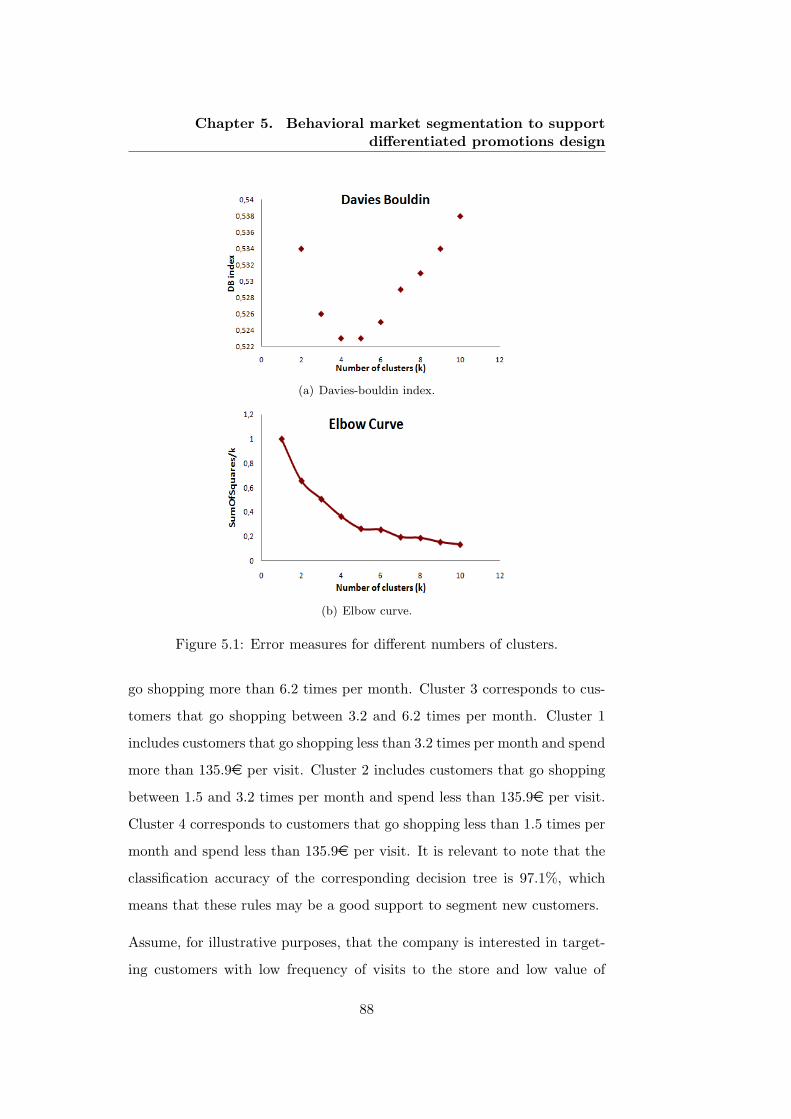
Chapter 5. Behavioral market segmentation to supportdifferentiated promotions design
(a) Davies-bouldin index.
(b) Elbow curve.
Figure 5.1: Error measures for different numbers of clusters.
go shopping more than 6.2 times per month. Cluster 3 corresponds to cus-
tomers that go shopping between 3.2 and 6.2 times per month. Cluster 1
includes customers that go shopping less than 3.2 times per month and spend
more than 135.9e per visit. Cluster 2 includes customers that go shopping
between 1.5 and 3.2 times per month and spend less than 135.9e per visit.
Cluster 4 corresponds to customers that go shopping less than 1.5 times per
month and spend less than 135.9e per visit. It is relevant to note that the
classification accuracy of the corresponding decision tree is 97.1%, which
means that these rules may be a good support to segment new customers.
Assume, for illustrative purposes, that the company is interested in target-
ing customers with low frequency of visits to the store and low value of
88
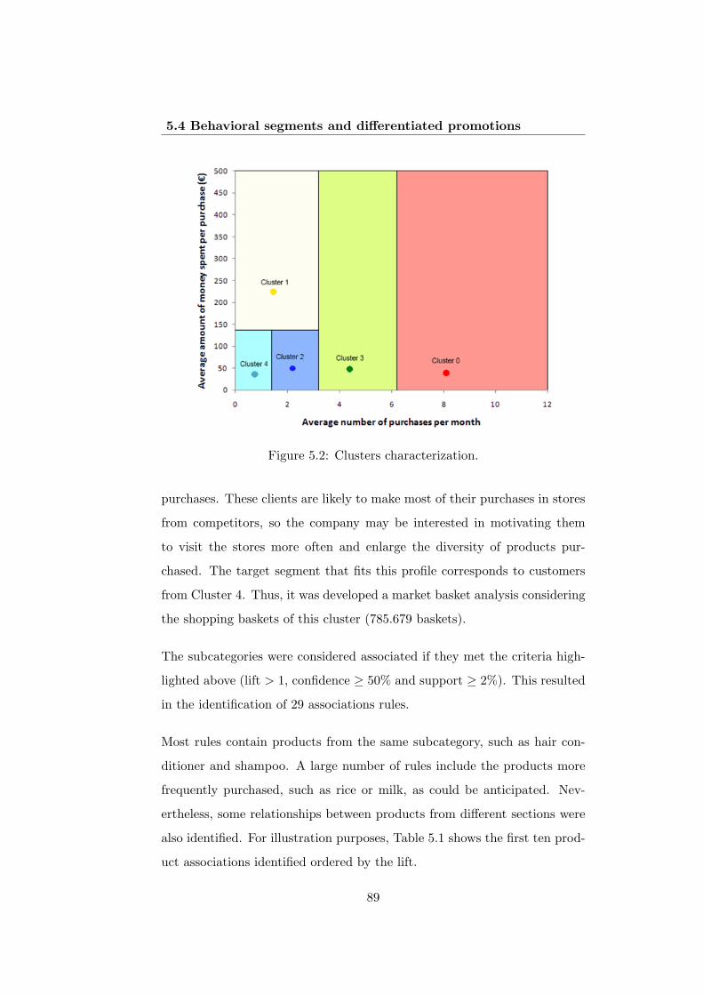
5.4 Behavioral segments and differentiated promotions
Figure 5.2: Clusters characterization.
purchases. These clients are likely to make most of their purchases in stores
from competitors, so the company may be interested in motivating them
to visit the stores more often and enlarge the diversity of products pur-
chased. The target segment that fits this profile corresponds to customers
from Cluster 4. Thus, it was developed a market basket analysis considering
the shopping baskets of this cluster (785.679 baskets).
The subcategories were considered associated if they met the criteria high-
lighted above (lift > 1, confidence ≥ 50% and support ≥ 2%). This resulted
in the identification of 29 associations rules.
Most rules contain products from the same subcategory, such as hair con-
ditioner and shampoo. A large number of rules include the products more
frequently purchased, such as rice or milk, as could be anticipated. Nev-
ertheless, some relationships between products from different sections were
also identified. For illustration purposes, Table 5.1 shows the first ten prod-
uct associations identified ordered by the lift.
89
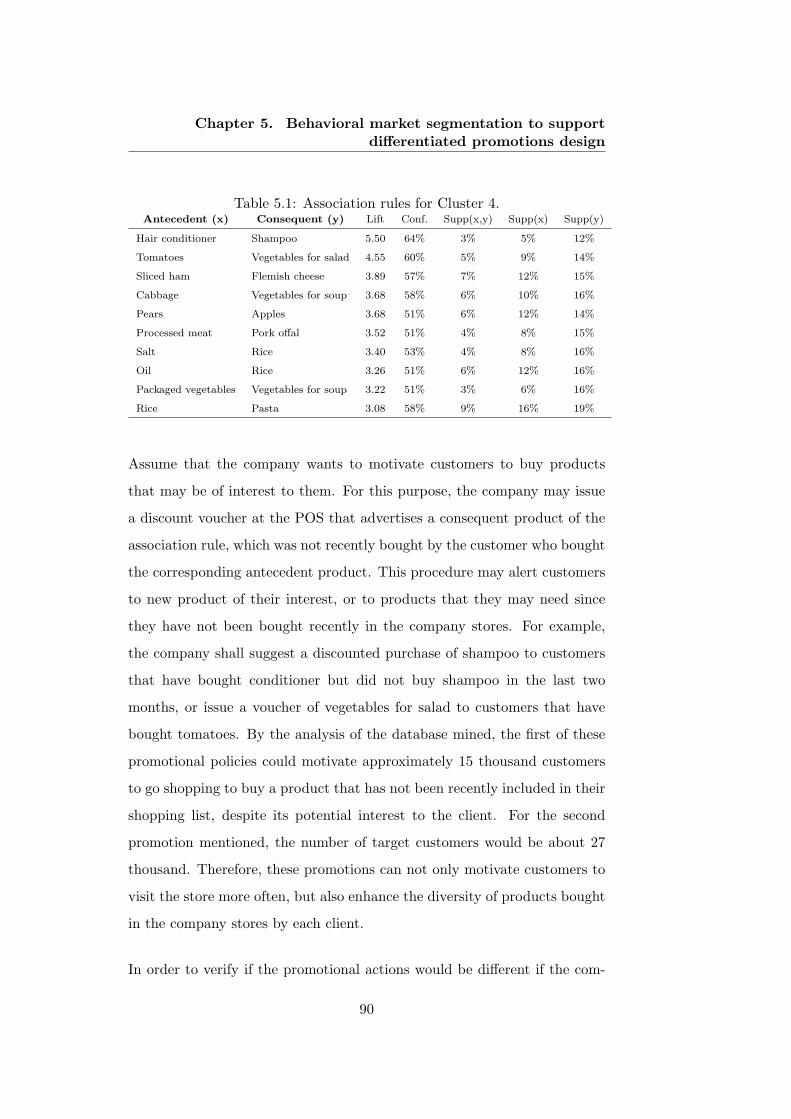
Chapter 5. Behavioral market segmentation to supportdifferentiated promotions design
Table 5.1: Association rules for Cluster 4.Antecedent (x) Consequent (y) Lift Conf. Supp(x,y) Supp(x) Supp(y)
Hair conditioner Shampoo 5.50 64% 3% 5% 12%
Tomatoes Vegetables for salad 4.55 60% 5% 9% 14%
Sliced ham Flemish cheese 3.89 57% 7% 12% 15%
Cabbage Vegetables for soup 3.68 58% 6% 10% 16%
Pears Apples 3.68 51% 6% 12% 14%
Processed meat Pork offal 3.52 51% 4% 8% 15%
Salt Rice 3.40 53% 4% 8% 16%
Oil Rice 3.26 51% 6% 12% 16%
Packaged vegetables Vegetables for soup 3.22 51% 3% 6% 16%
Rice Pasta 3.08 58% 9% 16% 19%
Assume that the company wants to motivate customers to buy products
that may be of interest to them. For this purpose, the company may issue
a discount voucher at the POS that advertises a consequent product of the
association rule, which was not recently bought by the customer who bought
the corresponding antecedent product. This procedure may alert customers
to new product of their interest, or to products that they may need since
they have not been bought recently in the company stores. For example,
the company shall suggest a discounted purchase of shampoo to customers
that have bought conditioner but did not buy shampoo in the last two
months, or issue a voucher of vegetables for salad to customers that have
bought tomatoes. By the analysis of the database mined, the first of these
promotional policies could motivate approximately 15 thousand customers
to go shopping to buy a product that has not been recently included in their
shopping list, despite its potential interest to the client. For the second
promotion mentioned, the number of target customers would be about 27
thousand. Therefore, these promotions can not only motivate customers to
visit the store more often, but also enhance the diversity of products bought
in the company stores by each client.
In order to verify if the promotional actions would be different if the com-
90
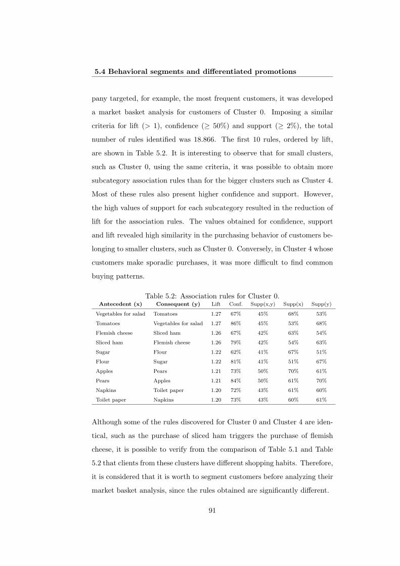
5.4 Behavioral segments and differentiated promotions
pany targeted, for example, the most frequent customers, it was developed
a market basket analysis for customers of Cluster 0. Imposing a similar
criteria for lift (> 1), confidence (≥ 50%) and support (≥ 2%), the total
number of rules identified was 18.866. The first 10 rules, ordered by lift,
are shown in Table 5.2. It is interesting to observe that for small clusters,
such as Cluster 0, using the same criteria, it was possible to obtain more
subcategory association rules than for the bigger clusters such as Cluster 4.
Most of these rules also present higher confidence and support. However,
the high values of support for each subcategory resulted in the reduction of
lift for the association rules. The values obtained for confidence, support
and lift revealed high similarity in the purchasing behavior of customers be-
longing to smaller clusters, such as Cluster 0. Conversely, in Cluster 4 whose
customers make sporadic purchases, it was more difficult to find common
buying patterns.
Table 5.2: Association rules for Cluster 0.Antecedent (x) Consequent (y) Lift Conf. Supp(x,y) Supp(x) Supp(y)
Vegetables for salad Tomatoes 1.27 67% 45% 68% 53%
Tomatoes Vegetables for salad 1.27 86% 45% 53% 68%
Flemish cheese Sliced ham 1.26 67% 42% 63% 54%
Sliced ham Flemish cheese 1.26 79% 42% 54% 63%
Sugar Flour 1.22 62% 41% 67% 51%
Flour Sugar 1.22 81% 41% 51% 67%
Apples Pears 1.21 73% 50% 70% 61%
Pears Apples 1.21 84% 50% 61% 70%
Napkins Toilet paper 1.20 72% 43% 61% 60%
Toilet paper Napkins 1.20 73% 43% 60% 61%
Although some of the rules discovered for Cluster 0 and Cluster 4 are iden-
tical, such as the purchase of sliced ham triggers the purchase of flemish
cheese, it is possible to verify from the comparison of Table 5.1 and Table
5.2 that clients from these clusters have different shopping habits. Therefore,
it is considered that it is worth to segment customers before analyzing their
market basket analysis, since the rules obtained are significantly different.
91
Chapter 5. Behavioral market segmentation to supportdifferentiated promotions design
5.5 Conclusion
This chapter segmented customers of the company used as case study and
proposed promotional policies tailored to customers from each segment, aim-
ing to reinforce loyal relationships.
Data mining allowed to find natural clusters based on transactional records
stored in the company loyalty card database. The segmentation was based
on a frequency (average number of purchases made per month) and mon-
etary value (average amount of money spent per purchase) criteria. Using
a partitioning cluster analysis technique, customers were grouped into five
clusters according to their shopping habits. The analysis also involved the
construction of a decision tree in order to extract the rules underlying cus-
tomer segmentation. Following this procedure, it was possible to draw a
profile for each segment that can be used for customers classification with
high precision.
The research described in this chapter also identified significant product
association rules within each segment, taking into account customers’ market
baskets. These rules enabled the design of differentiated promotions that
can be crucial to motivate customers to increase their purchases and keep
loyal to the company.
92
Chapter 6
Lifestyle marketsegmentation
6.1 Introduction
In this chapter customers identification is revisited. It is explored a different
method for market segmentation based on customers’ lifestyle. Instead of
segmenting customers based on the amount and frequency of their purchases,
they are grouped based on the kind of products they buy. To achieve this
purpose, a set of shopping baskets are mined and these are used to infer
customer lifestyle. Customers are assigned to a lifestyle segment based on
the history of their purchases. This chapter also suggests some marketing
actions to reinforce the relationship between companies and customers.
The structure of the remainder of this chapter is as follows. Section 6.2
includes a presentation of the methodology. Section 6.3 discusses the seg-
mentation results and Section 6.4 suggests marketing actions based on the
lifestyle segmentation. Section 6.5 presents the main conclusions.
93
Chapter 6. Lifestyle market segmentation
6.2 Methodology
The methodology described in this chapter aims to segment customers based
on their lifestyle, inferred from transactional records. To achieve this pur-
pose, typical shopping baskets were first identified by using a clustering
technique, which enabled to group the products more frequently purchased
together. In the context of this analysis, a shopping basket was defined as
the set of distinct products bought by a customer over the period consid-
ered. Since it was believed that the content of the shopping baskets defines
customers’ lifestyle, lifestyle segments were inferred by analyzing the typ-
ical shopping baskets. Customers were then assigned to the segments by
considering the history of their purchases.
Clustering analysis is a widely used data mining technique that maps data
items into unknown groups of items with high similarity (i.e., clusters).
There is a large variety of clustering algorithms available, as discussed in
Chapter 3. Since it was intended to discover lifestyle profiles, which can
be more stable than customers’ groups, the procedure used integrated a
variable clustering algorithm instead of a clustering algorithm for customers.
The algorithm used in this study is the most popular variable clustering
algorithm, i.e. varclus algorithm (see Chapter 3 for further details). In
this study the variables were the products, and consequently the resulting
clusters were typical shopping baskets.
Having obtained the clusters of products, the features of the products be-
longing to each cluster were analyzed in order to infer the lifestyle of cus-
tomers who usually bought those products. The granularity of the products
classification (e.g. department, business unit or category) considered in the
analysis should enable a general characterization of the shopping basket and,
consequently, the level of the analysis was the business unit and category,
as more detail was considered unnecessary.
94
6.3 Lifestyle segments
After having identified the lifestyle segments, each customer was assigned to
the lifestyle segment whose typical shopping basket presented more products
in common with the customer shopping basket corresponding to past trans-
actions. For this purpose, it was used a binary matrix revealing whether a
customer bought a product, and the total number of products that each cus-
tomer bought from each cluster was calculated. Note that, as it is believed
that the lifestyles are determined by the type of products bought, rather
than the quantities bought, the matrix was not prepared with information
on the value of the purchases. The customers were then assigned to the
cluster whose products were most similar to the customer past purchases.
6.3 Lifestyle segments
The analysis reported in this chapter is based on the Database 1 presented
in Section 4.4. From this data, 100.000 customers were randomly selected
to be used for the variable clustering procedure. Since the study should be
focused on the representative products in terms of sales, from the 105.160
different products transacted only those bought by at least 10.000 customers,
i.e. 1831 products, were selected. From the transaction records, it was then
created a binary matrix, which included as items the 100.000 customers (i.e.
1831 products). The binary structure of the matrix indicated whether a
customer bought each of the products or not.
In order to evaluate the number of clusters that would be appropriate to
use, the varclus algorithm was first run to obtain a dendrogram, as de-
picted in Figure 6.1. The number of clusters specified should ensure that
the segments were substantial (in the sense they should be large enough),
and differentiable (i.e., truly distinct from other segments). These criteria
are recognizable requirements for segments to be considered effective (Kotler
et al., 2003). By analyzing the dendrogram it was decided that the appro-
95
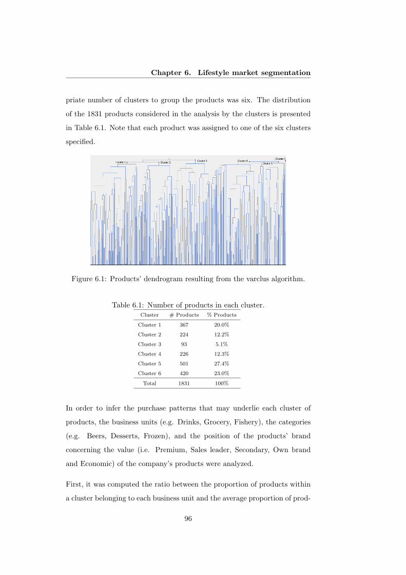
Chapter 6. Lifestyle market segmentation
priate number of clusters to group the products was six. The distribution
of the 1831 products considered in the analysis by the clusters is presented
in Table 6.1. Note that each product was assigned to one of the six clusters
specified.
Figure 6.1: Products’ dendrogram resulting from the varclus algorithm.
Table 6.1: Number of products in each cluster.Cluster # Products % Products
Cluster 1 367 20.0%
Cluster 2 224 12.2%
Cluster 3 93 5.1%
Cluster 4 226 12.3%
Cluster 5 501 27.4%
Cluster 6 420 23.0%
Total 1831 100%
In order to infer the purchase patterns that may underlie each cluster of
products, the business units (e.g. Drinks, Grocery, Fishery), the categories
(e.g. Beers, Desserts, Frozen), and the position of the products’ brand
concerning the value (i.e. Premium, Sales leader, Secondary, Own brand
and Economic) of the company’s products were analyzed.
First, it was computed the ratio between the proportion of products within
a cluster belonging to each business unit and the average proportion of prod-
96
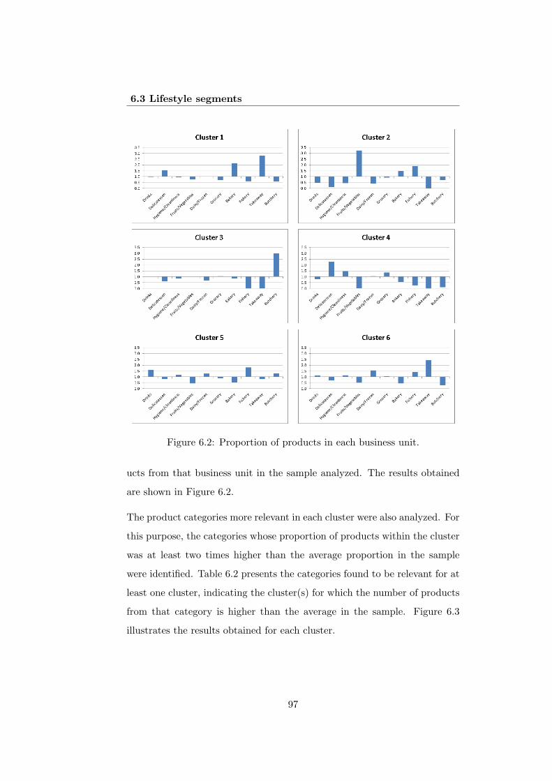
6.3 Lifestyle segments
Figure 6.2: Proportion of products in each business unit.
ucts from that business unit in the sample analyzed. The results obtained
are shown in Figure 6.2.
The product categories more relevant in each cluster were also analyzed. For
this purpose, the categories whose proportion of products within the cluster
was at least two times higher than the average proportion in the sample
were identified. Table 6.2 presents the categories found to be relevant for at
least one cluster, indicating the cluster(s) for which the number of products
from that category is higher than the average in the sample. Figure 6.3
illustrates the results obtained for each cluster.
97
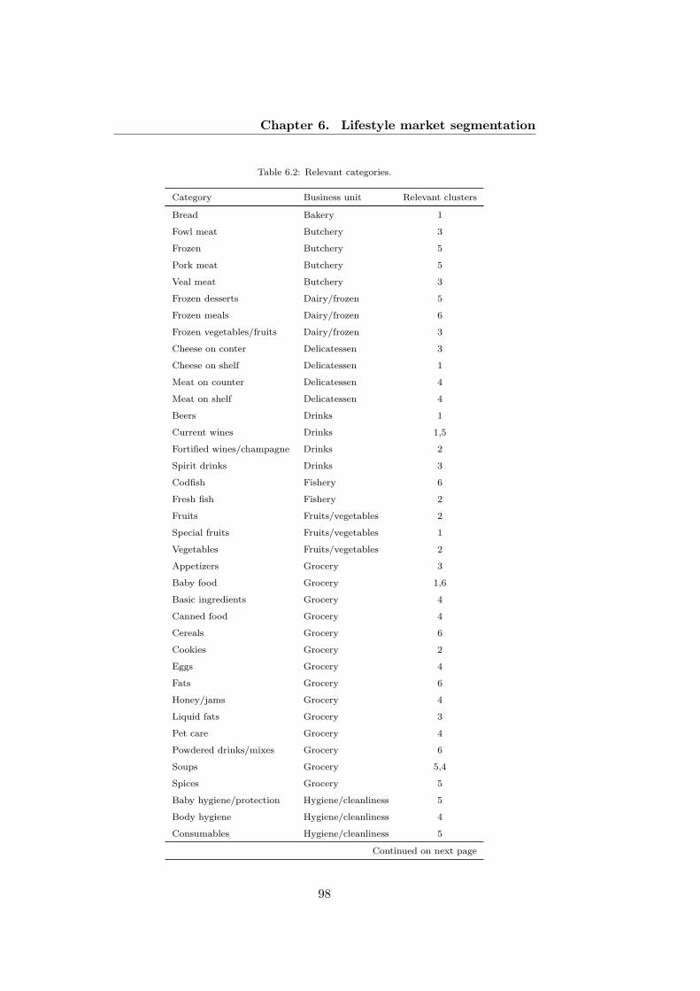
Chapter 6. Lifestyle market segmentation
Table 6.2: Relevant categories.
Category Business unit Relevant clusters
Bread Bakery 1
Fowl meat Butchery 3
Frozen Butchery 5
Pork meat Butchery 5
Veal meat Butchery 3
Frozen desserts Dairy/frozen 5
Frozen meals Dairy/frozen 6
Frozen vegetables/fruits Dairy/frozen 3
Cheese on conter Delicatessen 3
Cheese on shelf Delicatessen 1
Meat on counter Delicatessen 4
Meat on shelf Delicatessen 4
Beers Drinks 1
Current wines Drinks 1,5
Fortified wines/champagne Drinks 2
Spirit drinks Drinks 3
Codfish Fishery 6
Fresh fish Fishery 2
Fruits Fruits/vegetables 2
Special fruits Fruits/vegetables 1
Vegetables Fruits/vegetables 2
Appetizers Grocery 3
Baby food Grocery 1,6
Basic ingredients Grocery 4
Canned food Grocery 4
Cereals Grocery 6
Cookies Grocery 2
Eggs Grocery 4
Fats Grocery 6
Honey/jams Grocery 4
Liquid fats Grocery 3
Pet care Grocery 4
Powdered drinks/mixes Grocery 6
Soups Grocery 5,4
Spices Grocery 5
Baby hygiene/protection Hygiene/cleanliness 5
Body hygiene Hygiene/cleanliness 4
Consumables Hygiene/cleanliness 5
Continued on next page
98
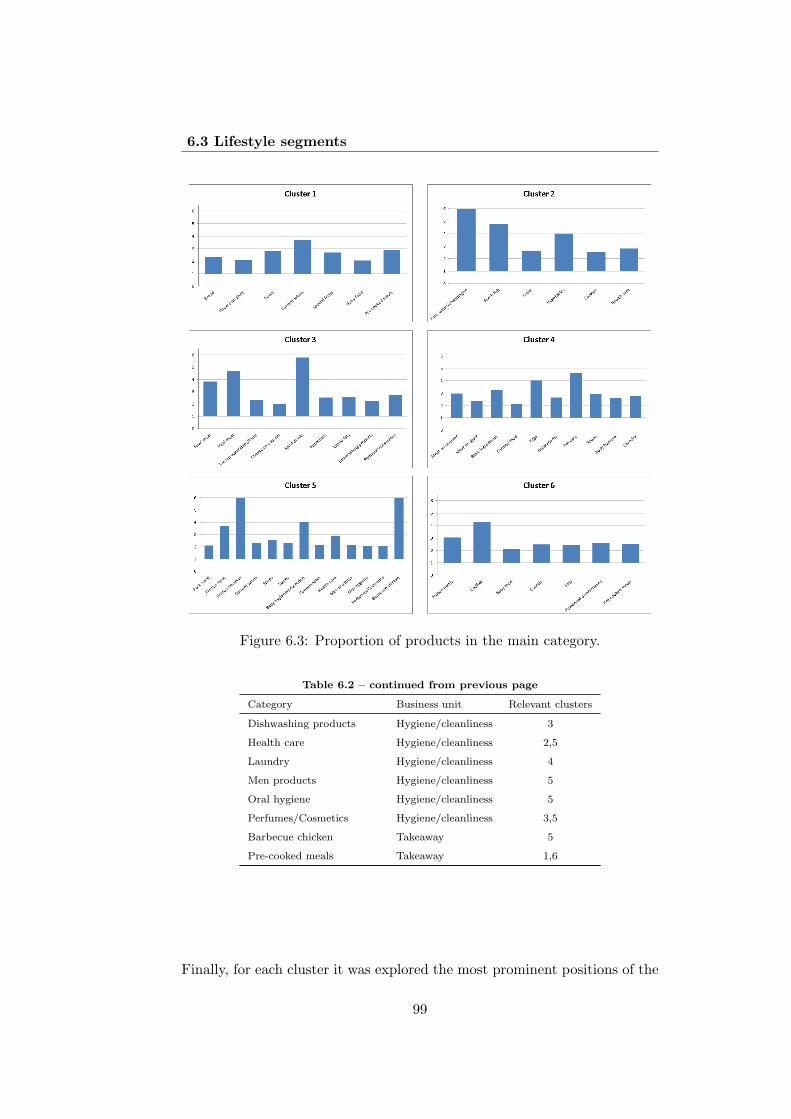
6.3 Lifestyle segments
Figure 6.3: Proportion of products in the main category.
Table 6.2 – continued from previous page
Category Business unit Relevant clusters
Dishwashing products Hygiene/cleanliness 3
Health care Hygiene/cleanliness 2,5
Laundry Hygiene/cleanliness 4
Men products Hygiene/cleanliness 5
Oral hygiene Hygiene/cleanliness 5
Perfumes/Cosmetics Hygiene/cleanliness 3,5
Barbecue chicken Takeaway 5
Pre-cooked meals Takeaway 1,6
Finally, for each cluster it was explored the most prominent positions of the
99
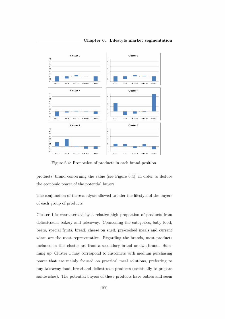
Chapter 6. Lifestyle market segmentation
Figure 6.4: Proportion of products in each brand position.
products’ brand concerning the value (see Figure 6.4), in order to deduce
the economic power of the potential buyers.
The conjunction of these analysis allowed to infer the lifestyle of the buyers
of each group of products.
Cluster 1 is characterized by a relative high proportion of products from
delicatessen, bakery and takeaway. Concerning the categories, baby food,
beers, special fruits, bread, cheese on shelf, pre-cooked meals and current
wines are the most representative. Regarding the brands, most products
included in this cluster are from a secondary brand or own-brand. Sum-
ming up, Cluster 1 may correspond to customers with medium purchasing
power that are mainly focused on practical meal solutions, preferring to
buy takeaway food, bread and delicatessen products (eventually to prepare
sandwiches). The potential buyers of these products have babies and seem
100
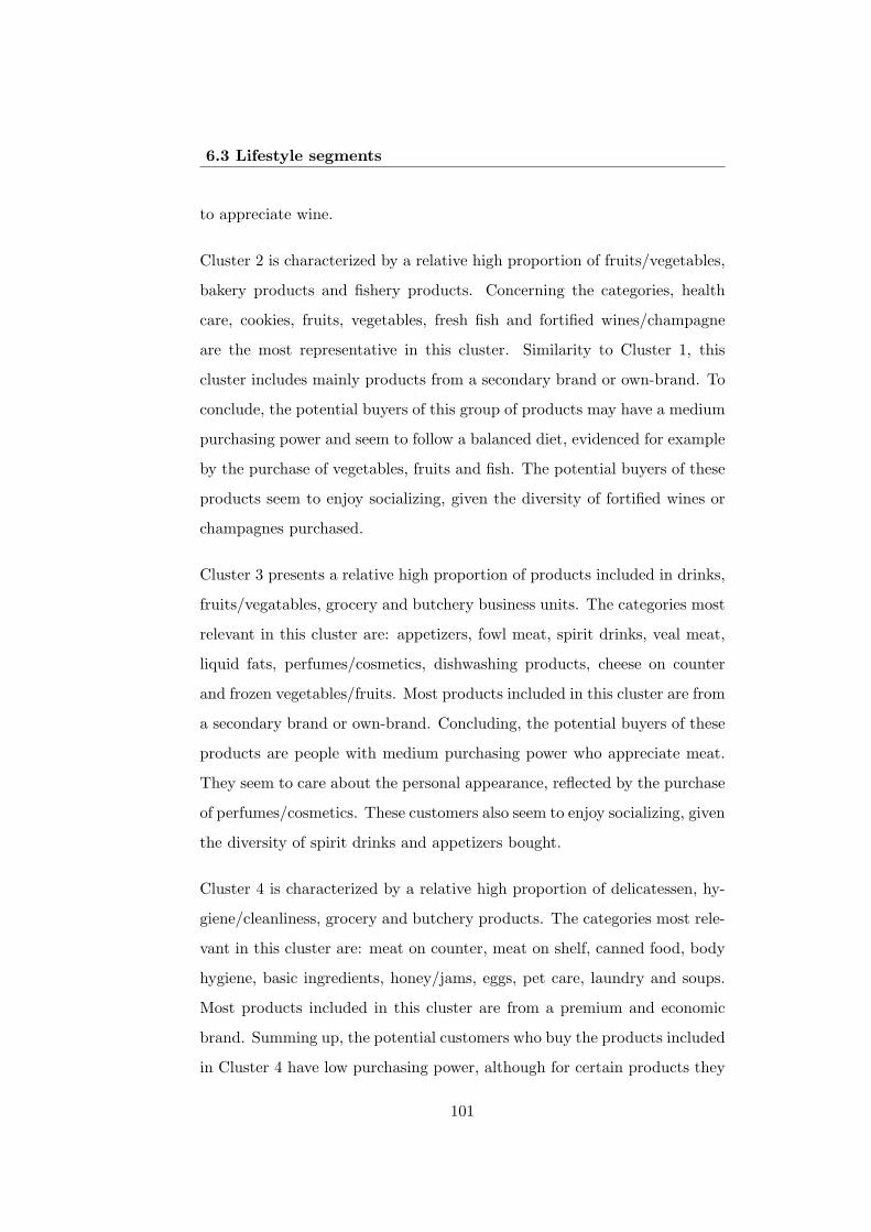
6.3 Lifestyle segments
to appreciate wine.
Cluster 2 is characterized by a relative high proportion of fruits/vegetables,
bakery products and fishery products. Concerning the categories, health
care, cookies, fruits, vegetables, fresh fish and fortified wines/champagne
are the most representative in this cluster. Similarity to Cluster 1, this
cluster includes mainly products from a secondary brand or own-brand. To
conclude, the potential buyers of this group of products may have a medium
purchasing power and seem to follow a balanced diet, evidenced for example
by the purchase of vegetables, fruits and fish. The potential buyers of these
products seem to enjoy socializing, given the diversity of fortified wines or
champagnes purchased.
Cluster 3 presents a relative high proportion of products included in drinks,
fruits/vegatables, grocery and butchery business units. The categories most
relevant in this cluster are: appetizers, fowl meat, spirit drinks, veal meat,
liquid fats, perfumes/cosmetics, dishwashing products, cheese on counter
and frozen vegetables/fruits. Most products included in this cluster are from
a secondary brand or own-brand. Concluding, the potential buyers of these
products are people with medium purchasing power who appreciate meat.
They seem to care about the personal appearance, reflected by the purchase
of perfumes/cosmetics. These customers also seem to enjoy socializing, given
the diversity of spirit drinks and appetizers bought.
Cluster 4 is characterized by a relative high proportion of delicatessen, hy-
giene/cleanliness, grocery and butchery products. The categories most rele-
vant in this cluster are: meat on counter, meat on shelf, canned food, body
hygiene, basic ingredients, honey/jams, eggs, pet care, laundry and soups.
Most products included in this cluster are from a premium and economic
brand. Summing up, the potential customers who buy the products included
in Cluster 4 have low purchasing power, although for certain products they
101
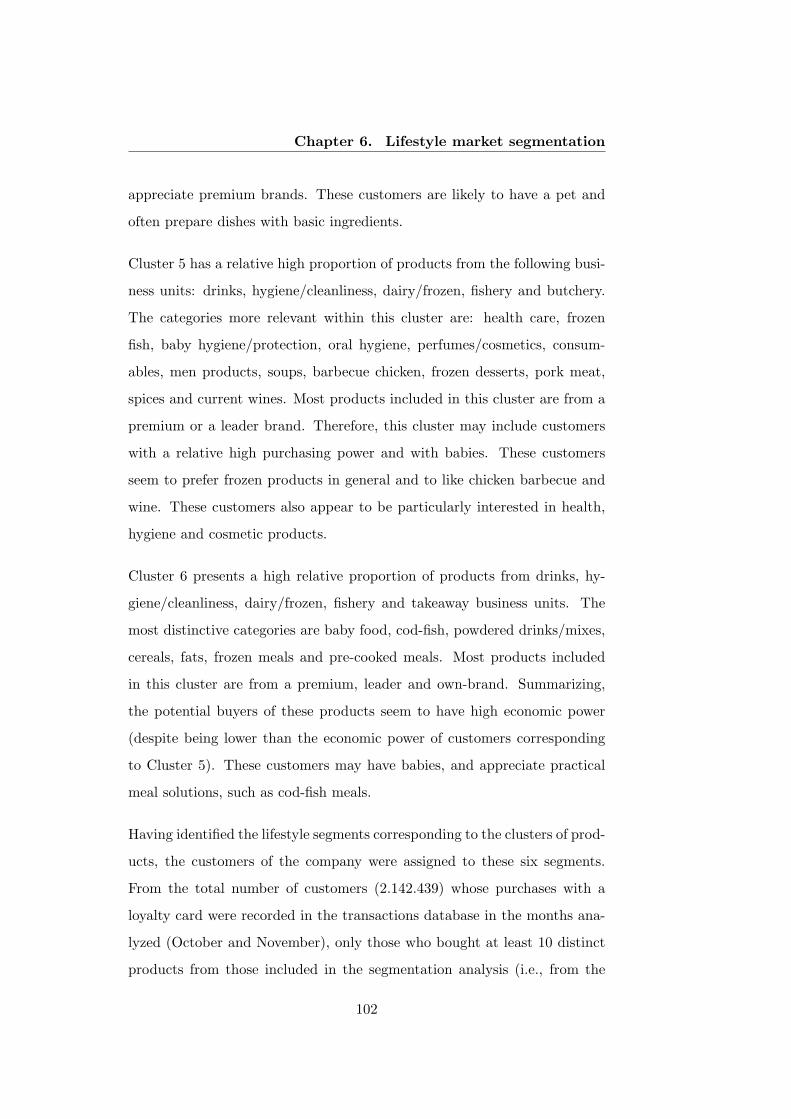
Chapter 6. Lifestyle market segmentation
appreciate premium brands. These customers are likely to have a pet and
often prepare dishes with basic ingredients.
Cluster 5 has a relative high proportion of products from the following busi-
ness units: drinks, hygiene/cleanliness, dairy/frozen, fishery and butchery.
The categories more relevant within this cluster are: health care, frozen
fish, baby hygiene/protection, oral hygiene, perfumes/cosmetics, consum-
ables, men products, soups, barbecue chicken, frozen desserts, pork meat,
spices and current wines. Most products included in this cluster are from a
premium or a leader brand. Therefore, this cluster may include customers
with a relative high purchasing power and with babies. These customers
seem to prefer frozen products in general and to like chicken barbecue and
wine. These customers also appear to be particularly interested in health,
hygiene and cosmetic products.
Cluster 6 presents a high relative proportion of products from drinks, hy-
giene/cleanliness, dairy/frozen, fishery and takeaway business units. The
most distinctive categories are baby food, cod-fish, powdered drinks/mixes,
cereals, fats, frozen meals and pre-cooked meals. Most products included
in this cluster are from a premium, leader and own-brand. Summarizing,
the potential buyers of these products seem to have high economic power
(despite being lower than the economic power of customers corresponding
to Cluster 5). These customers may have babies, and appreciate practical
meal solutions, such as cod-fish meals.
Having identified the lifestyle segments corresponding to the clusters of prod-
ucts, the customers of the company were assigned to these six segments.
From the total number of customers (2.142.439) whose purchases with a
loyalty card were recorded in the transactions database in the months ana-
lyzed (October and November), only those who bought at least 10 distinct
products from those included in the segmentation analysis (i.e., from the
102
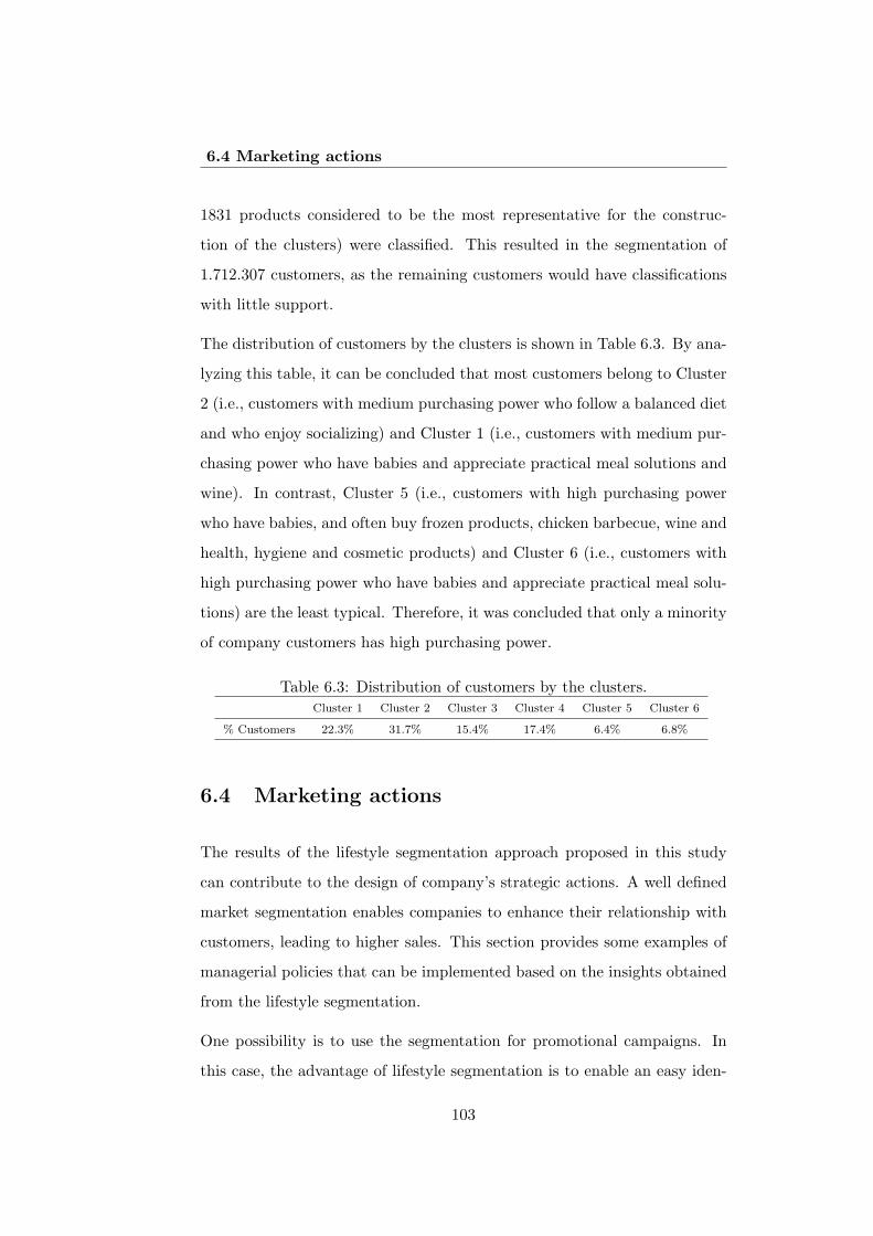
6.4 Marketing actions
1831 products considered to be the most representative for the construc-
tion of the clusters) were classified. This resulted in the segmentation of
1.712.307 customers, as the remaining customers would have classifications
with little support.
The distribution of customers by the clusters is shown in Table 6.3. By ana-
lyzing this table, it can be concluded that most customers belong to Cluster
2 (i.e., customers with medium purchasing power who follow a balanced diet
and who enjoy socializing) and Cluster 1 (i.e., customers with medium pur-
chasing power who have babies and appreciate practical meal solutions and
wine). In contrast, Cluster 5 (i.e., customers with high purchasing power
who have babies, and often buy frozen products, chicken barbecue, wine and
health, hygiene and cosmetic products) and Cluster 6 (i.e., customers with
high purchasing power who have babies and appreciate practical meal solu-
tions) are the least typical. Therefore, it was concluded that only a minority
of company customers has high purchasing power.
Table 6.3: Distribution of customers by the clusters.Cluster 1 Cluster 2 Cluster 3 Cluster 4 Cluster 5 Cluster 6
% Customers 22.3% 31.7% 15.4% 17.4% 6.4% 6.8%
6.4 Marketing actions
The results of the lifestyle segmentation approach proposed in this study
can contribute to the design of company’s strategic actions. A well defined
market segmentation enables companies to enhance their relationship with
customers, leading to higher sales. This section provides some examples of
managerial policies that can be implemented based on the insights obtained
from the lifestyle segmentation.
One possibility is to use the segmentation for promotional campaigns. In
this case, the advantage of lifestyle segmentation is to enable an easy iden-
103
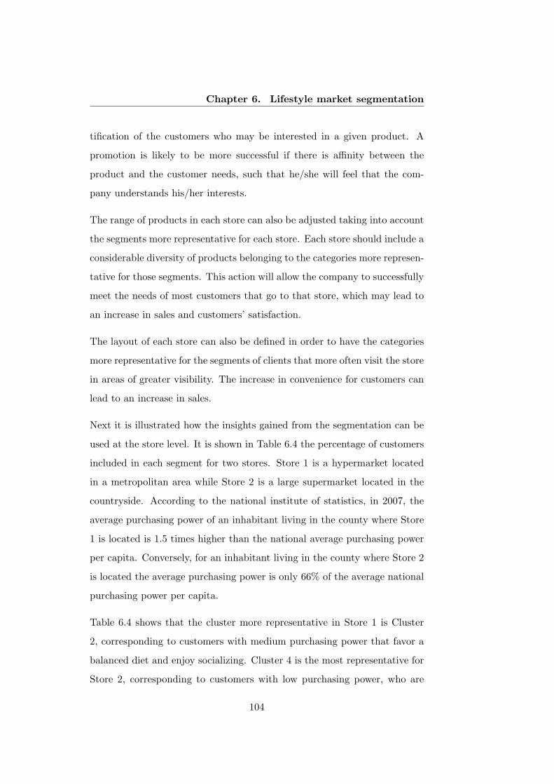
Chapter 6. Lifestyle market segmentation
tification of the customers who may be interested in a given product. A
promotion is likely to be more successful if there is affinity between the
product and the customer needs, such that he/she will feel that the com-
pany understands his/her interests.
The range of products in each store can also be adjusted taking into account
the segments more representative for each store. Each store should include a
considerable diversity of products belonging to the categories more represen-
tative for those segments. This action will allow the company to successfully
meet the needs of most customers that go to that store, which may lead to
an increase in sales and customers’ satisfaction.
The layout of each store can also be defined in order to have the categories
more representative for the segments of clients that more often visit the store
in areas of greater visibility. The increase in convenience for customers can
lead to an increase in sales.
Next it is illustrated how the insights gained from the segmentation can be
used at the store level. It is shown in Table 6.4 the percentage of customers
included in each segment for two stores. Store 1 is a hypermarket located
in a metropolitan area while Store 2 is a large supermarket located in the
countryside. According to the national institute of statistics, in 2007, the
average purchasing power of an inhabitant living in the county where Store
1 is located is 1.5 times higher than the national average purchasing power
per capita. Conversely, for an inhabitant living in the county where Store 2
is located the average purchasing power is only 66% of the average national
purchasing power per capita.
Table 6.4 shows that the cluster more representative in Store 1 is Cluster
2, corresponding to customers with medium purchasing power that favor a
balanced diet and enjoy socializing. Cluster 4 is the most representative for
Store 2, corresponding to customers with low purchasing power, who are
104
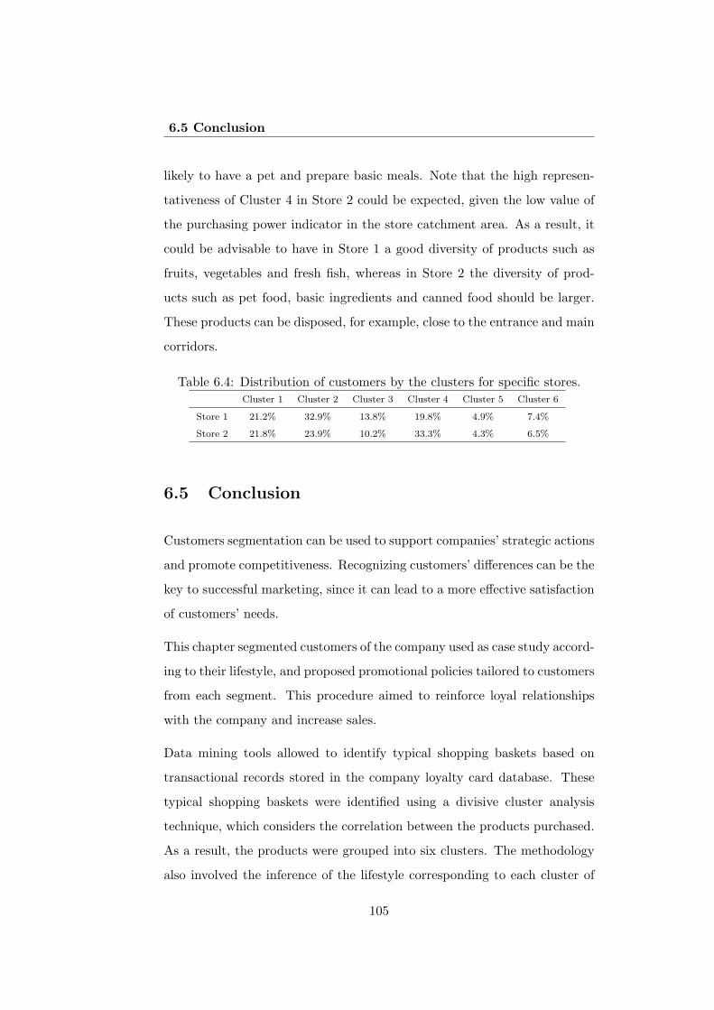
6.5 Conclusion
likely to have a pet and prepare basic meals. Note that the high represen-
tativeness of Cluster 4 in Store 2 could be expected, given the low value of
the purchasing power indicator in the store catchment area. As a result, it
could be advisable to have in Store 1 a good diversity of products such as
fruits, vegetables and fresh fish, whereas in Store 2 the diversity of prod-
ucts such as pet food, basic ingredients and canned food should be larger.
These products can be disposed, for example, close to the entrance and main
corridors.
Table 6.4: Distribution of customers by the clusters for specific stores.Cluster 1 Cluster 2 Cluster 3 Cluster 4 Cluster 5 Cluster 6
Store 1 21.2% 32.9% 13.8% 19.8% 4.9% 7.4%
Store 2 21.8% 23.9% 10.2% 33.3% 4.3% 6.5%
6.5 Conclusion
Customers segmentation can be used to support companies’ strategic actions
and promote competitiveness. Recognizing customers’ differences can be the
key to successful marketing, since it can lead to a more effective satisfaction
of customers’ needs.
This chapter segmented customers of the company used as case study accord-
ing to their lifestyle, and proposed promotional policies tailored to customers
from each segment. This procedure aimed to reinforce loyal relationships
with the company and increase sales.
Data mining tools allowed to identify typical shopping baskets based on
transactional records stored in the company loyalty card database. These
typical shopping baskets were identified using a divisive cluster analysis
technique, which considers the correlation between the products purchased.
As a result, the products were grouped into six clusters. The methodology
also involved the inference of the lifestyle corresponding to each cluster of
105
Chapter 6. Lifestyle market segmentation
products, by analyzing the type of products included in each cluster. In par-
ticular, it was analyzed the business unit, the category and the position of
the product brand concerning the value. Each customer was then assigned
to the segment whose shopping basket was more similar to the customer’s
past purchases. The research described in this chapter also identified some
marketing actions, such as differentiated promotional campaigns, adjust-
ment of stores’ range of products and adjustment of stores’ layout, that can
help to reinforce the relationship between companies and customers.
106
Chapter 7
Partial customer churnprediction using products’first purchase sequence
7.1 Introduction
Customers retention has deserved particular attention in the grocery re-
tail sector. This topic is addressed in this chapter by developing a churn
prediction model. This model includes as an explanatory variable the sim-
ilarity of the sequences of the first products purchased with churner’s and
non-churner’s sequences. The sequence of first purchase events is modeled
using markov-for-discrimination. Two classification techniques are used in
the empirical study: logistic regression and random forests.
The structure of the remainder of the chapter is as follows. Section 7.2
presents the motivation for this study. Section 7.2 includes a brief revision
of churn prediction modeling in the literature. Section 7.4 introduces the
methodology followed in this study, namely the explanatory variables used
and the performance evaluation criteria used. Section 7.5 presents the results
and introduces some ideas of retention campaigns. The chapter finishes with
107
Chapter 7. Partial customer churn prediction using products’first purchase sequence
the conclusion.
7.2 Customers retention
As mentioned in Chapter 2, customer relationship management can be sum-
marized as the combination of four dimensions: customer identification,
customer attraction, customer development and customer retention. In to-
day’s competitive environment, customer retention is receiving particular
attention from companies, as customer life cycles are becoming shorter than
in the past. Some customers present switching behavior in their purchases
(Peterson, 1995) and others split their purchases between several competi-
tors (Dwyer, 1989). Particularly in non-contractual settings, such as the
retail sector, this tendency is of utmost relevance, since customers do not
have to inform companies about their churn intention and experience very
little switching cost. According to EFMI and CBL (2005), a total of 87%
of grocery shoppers use two or more different supermarkets for their gro-
cery shopping and, on average, those grocery shoppers visit 2.8 different
supermarkets each month.
Companies’ concern about customer churn is based on the benefits associ-
ated with retaining customers. Previous research suggests that retaining
customers costs less than attracting new customers (Dick and Basu, 1994;
Saren and Tzokas, 1998). Moreover, when the relationship between com-
panies and customers is strong, these customers tend to be less sensitive
to competitors’ actions (Strandvik and Liljander, 1994) and prices (Kotler,
1999), and are less costly to serve (Bejou et al., 1998). These customers
present an important role in the word-of-mouth (WOM) process (Martin
et al., 1995) and show high purchase levels (Kamakura et al., 1991). In this
context, a small improvement in customer retention can mean a significant
increase in profit (Reichheld and Sasser Jr., 1990; Larivire and Van den Poel,
108
7.3 Churn prediction modeling
2005). Despite all the advantages associated with retaining customers, churn
analysis in retailing can still be considered incipient (Buckinx and Van den
Poel, 2005).
Churn problems presented in the literature differ in terms of the explanatory
variables considered. Buckinx and Van den Poel (2005) classifies defection
explanatory variables, or predictors, using three categories: behavioral an-
tecedents, demographics and perceptions. This study seeks to introduce a
new churn predictor, which measures the similarity of the sequences of the
first products purchased with churner’s and non-churner’s sequences. These
sequences of first purchase events are modeled as a markov process. More-
over, unlike most of the previous churn models proposed in the literature,
this study proposes a churn prediction model that identifies the customers
that are likely to partially leave the company. Furthermore, the empiri-
cal study compares the predictive performance of the models supported by
logistic regression and random forests.
7.3 Churn prediction modeling
Customer retention, and more specifically customer churn, has been widely
discussed in the literature in the last decade. For an overview on churn pre-
diction see Verbeke et al. (2011). Customer churn prediction models aim to
detect customers which are easily persuaded to discontinue the relationship
with the company. An accurate identification of these potential churners
allows companies to target them in retention marketing campaigns. This
topic has been studied in several domains and, in most cases, it is treated as
total defection. In banking (e.g. Kumar and Ravi, 2008; Larivire and Van
den Poel, 2005) and insurance (e.g. Zeithaml et al., 1996; Morik and Kpcke,
2004)) churn is usually seen as account closure. In telecommunications (e.g.
Hwang et al., 2004; Hung et al., 2006) it is usually seen as changing phone
109
Chapter 7. Partial customer churn prediction using products’first purchase sequence
operator. In retailing, to the best of the author’s knowledge, only Buckinx
and Van den Poel (2005) and Burez and Van den Poel (2009) have analyzed
churn. In both cases, churn was treated as partial churn since typically
customers defect from companies progressively, rather than in an abrupt
discontinuation. Buckinx and Van den Poel (2005) consider that in the long
run partial churn may result in total defection.
Churn prediction problems may be decomposed primarily into the choice of
the churn prediction techniques to be used and the definition of the churn
prediction model. The model requires the identification of the explanatory
variables which are relevant for the churn propensity. Furthermore, it in-
cludes the definition of the causality/link between these variables and the
churn.
A wide diversity of data mining classification techniques have been used as
churn prediction techniques (for an overview, see Verbeke et al., 2011). As
mentioned in Chapter 3, neural networks proposed by Mcculloch and Pitts
(1943) have frequently been used in this context (e.g. Hung et al., 2006;
Hwang et al., 2004). Neural networks are analytical tools, inspired by the
neural aspect of the human brain, which use simple processing units, linked
to each other through weighted connections, to “learn” the relationships be-
tween variables. Despite usually presenting good performance, these tools
are criticized for the fact they do not present the patterns underlying the
data, being characterized as black boxes (Paruelo and Tomasel, 1997). De-
cision trees, first introduced by Quinlan (1992), are also frequently used in
churn prediction by inducing a tree and subsequently extracting the rules
that can be used to identify the defectors (e.g. Wei and Chiu, 2002; Hung
et al., 2006). Rule inference is considered one of the advantages of this tech-
nique, while the lack of robustness and suboptimal performance are high-
lighted as disadvantages (Murthy, 1997). In order to deal with decision tree
disadvantages, random forests (Breiman, 2001) have become popular (e.g.
110
7.3 Churn prediction modeling
Buckinx and Van den Poel, 2005; Coussement and Van den Poel, 2008).
Their classification is based on an ensemble of trees, avoiding misclassifica-
tions due to the weak robustness and sub-optimality of a single decision tree.
The random forests technique allows a measure of the importance of each
variable for the classification to be obtained. This technique is considered
easy to use and provides robust results (Buckinx and Van den Poel, 2005).
Despite having been extensively studied, no general consensus exists on the
relative performance of churn prediction techniques. There are studies in
which one technique outperforms the other and vice versa (Verbeke et al.,
2011).
Concerning churn prediction variables, the churn prediction models pre-
sented in the literature also differ considerably (see Buckinx and Van den
Poel, 2005, for an overview). Perception variables are used in some studies
and try to measure the way a customer appreciates the service/product of
the company. They can be measured through customer surveys and include
dimensions such as overall satisfaction, quality of service, locational conve-
nience and reputation of the company. Most studies focus on demographic
predictors, such as age, gender, education, social status and geographical
data. A considerable number of prior studies also include behavioral an-
tecedent variables. The number of purchases (frequency) and the amount
of money spent (monetary value) are the most popular behavioral variables.
Buckinx and Van den Poel (2005) concludes that, in addition to these two
variables, recency is also part of the best-predictor group of variables. De-
spite having been disregarded in the literature, one behavioral dimension
that seems to have huge potential concerning customer attrition detection is
the purchase sequence of products. As stated by Grover and Vriens (2006),
customers seem to follow purchasing patterns similar to other customers, by
observing the purchasing behavior of other customers or due to the word-
of-mouth effects (Bikhchandani et al., 1992, 1998) resulting from communi-
111
Chapter 7. Partial customer churn prediction using products’first purchase sequence
cation with other customers. As a result, one customer can follow a similar
sequence to past customers, allowing companies to model their behavior (e.g.
Prinzie and Van den Poel, 2006; Prinzie and Van den Poel, 2006). In partic-
ular, the sequence of the first product purchased expresses the development
of the relationship of trust between a customer and the company and con-
sequent demand maturity. Typically, new customers have little knowledge
of the products they are trying to buy. Most customers will try to reduce
risk in this situation and consequently establish goal hierarchies (Novemsky
and Dhar, 2005). By doing so, customers break down the purchase process
into portions which can take a share of the risk. Usually, people only take
risks with later goals if the earlier goals in the sequence were accomplished
successfully (Dhar and Novemsky, 2002). Therefore, it is considered that
the level of similarity between the first products’ purchase sequence, chosen
by a new customer, and the sequence chosen by churners and non-churners
may be an indicator of the readiness of customers to churn or not. Thus,
this study hypothesizes that the sequence of the first products purchased by
the new customers may support churner and non-churner discrimination.
7.4 Methodology
The methodology followed in this chapter seeks to introduce and explore the
predictive power of a measure of the similarity of the sequences of the first
products purchased by the new customers with the corresponding sequences
recorded for churners and non-churners. The sequences were modeled in
terms of products’ business unit and the similarity measure was obtained by
using markov-for-discrimination (described in Section 7.4.2). The value of
the proposed predictor was assessed by comparing the accuracy obtained by
the model including the similarity variables with the accuracy obtained by
the model excluding these variables. Two data mining classification tech-
112
7.4 Methodology
niques were used and compared in the empirical study: logistic regression
and random forests. These techniques were chosen due to their robustness
and ease of application. The ability to handle non-linear effects also moti-
vated their use.
7.4.1 Partial churning
Since the model proposed in this chapter is intended to identify customers
who may partially switch their purchases to another company and since in
non-contractual businesses the defection is not explicit, it was necessary to
derive the dependent variable of the models. For this purpose, the purchases
were first grouped in periods of three months. Then, those customers who,
from a certain period, made no further transactions or those customers who
in all subsequent periods spent less than 40% of the amount spent in the
reference period, were classified as partial churners. The granularity of the
analysis and the amount spent threshold used was the result of a sensitivity
analysis. It was verified the impact of a higher/lower temporal aggregation
and the impact of the variation of the threshold on the proportion of par-
tial churners identified. The churn proportion considered realistic by the
business domain experts dictated these parameters.
Figure 7.1 represents the amount spent by two customers over five quarters.
The first case represents a customer who partially churned. Notably, when
the 2nd quarter is considered as the reference quarter, it is observed that
in all subsequent quarters this customer spent less than 40% of the amount
spent in the reference quarter (100e×40%=40e). Therefore, it is assumed
that this customer partially churned in the beginning of the 3rd quarter.
Concerning the second case, there is not any quarter in which the amount
spent in all subsequent quarters is less than 40% of the amount spent in the
reference quarter. Thus, this represents a customer who did not churn.
113
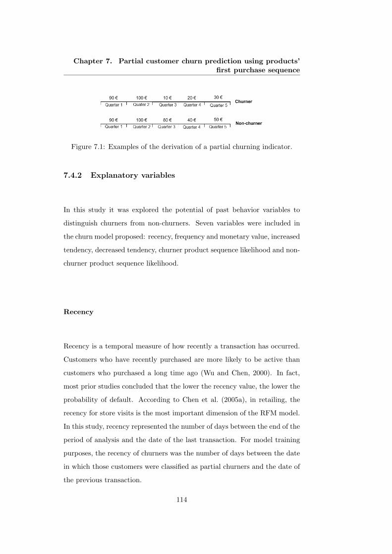
Chapter 7. Partial customer churn prediction using products’first purchase sequence
Figure 7.1: Examples of the derivation of a partial churning indicator.
7.4.2 Explanatory variables
In this study it was explored the potential of past behavior variables to
distinguish churners from non-churners. Seven variables were included in
the churn model proposed: recency, frequency and monetary value, increased
tendency, decreased tendency, churner product sequence likelihood and non-
churner product sequence likelihood.
Recency
Recency is a temporal measure of how recently a transaction has occurred.
Customers who have recently purchased are more likely to be active than
customers who purchased a long time ago (Wu and Chen, 2000). In fact,
most prior studies concluded that the lower the recency value, the lower the
probability of default. According to Chen et al. (2005a), in retailing, the
recency for store visits is the most important dimension of the RFM model.
In this study, recency represented the number of days between the end of the
period of analysis and the date of the last transaction. For model training
purposes, the recency of churners was the number of days between the date
in which those customers were classified as partial churners and the date of
the previous transaction.
114
7.4 Methodology
Frequency
Frequency is a measure of the strength of the customer relationship with
the company. Loyal customers, by definition, purchase more often than dis-
loyal customers (Kamakura et al., 1991). Berry and Linoff (2004) identify
frequency as a significant predictor of churn. Frequency was included in the
model proposed as the average number of transactions per quarter. Regard-
ing customers who churned partially, for model training purposes, frequency
was naturally calculated by considering only the transactions observed up
to the date in which those customers were classified as partial churners.
Monetary value
Monetary value is a measure of the expenditure of customers at a certain
company. According to Schmittlein and Peterson (1994), the monetary value
of each customer’s past purchases can be an important predictor of future
behavior. This RFM dimension was covered in this study by the average
value spent by customers in each quarter. As regards the partial churners
used for training the model, this variable only took into account the amount
spent up to the date they were classified as partial churners.
Increase or decrease tendency
As reported by Wei and Chiu (2002), more recent behavior should be more
useful for churn prediction than past behavior, since the time interval be-
tween intention to churn and action may not be very long. The model
proposed included two dummy variables that captured the recent changes
in customers’ behavior. Therefore, if a customer increased the amount of
money spent in the last quarter of the period analyzed in relation to the
amount spent in the previous quarter, the variable increased tendency took
the value 1, while the variable decreased tendency took the value 0. The
115
Chapter 7. Partial customer churn prediction using products’first purchase sequence
opposite happened if a decrease in the amount spent was observed. Con-
cerning the partial churners used to train the model, these two variables
were defined by analyzing the tendency in the two quarters before churning.
Products sequence likelihood
It was assumed that the likelihood of the sequence of the first products’ busi-
ness unit purchased compared with the same sequence recorded for churners
and non-churners could reveal whether a customer was about to churn or
not. It was proposed a measure of this similarity by using markov-for-
discrimination introduced by Durbin et al. (1998) and used, for example, by
Prinzie and Van den Poel (2007) in a predictive purchase sequences context.
Consider a process whose states are defined by a discrete variable X(t), (t =
0, 1, 2, ...) according to a stochastic process. The process can be considered
a markov process if:
P [Xt = a|Xt−1 = b,Xt−2 = c, ..., X0 = d] = P [Xt = a|Xt−1 = b] (7.1)
In a markov model, the probability of Xt taking a certain value depends only
on the value of Xt−1. Each markov process can be represented by means
of a transition matrix. In the case of a process with N possible states, the
transition matrix is a NxN matrix defined as:
M = [pij ] (7.2)
Each element of the matrix represents the probability of the system evolving
from a state i, in period t, to another state j, in period t + 1. In this
study, the state variable Xt was considered to be the product business unit
that a customer purchased at the t-th store visit. Products’ business unit
116
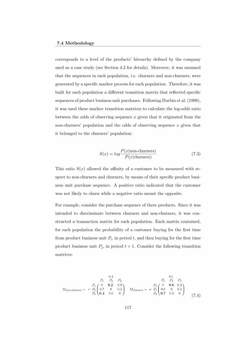
7.4 Methodology
corresponds to a level of the products’ hierarchy defined by the company
used as a case study (see Section 4.2 for details). Moreover, it was assumed
that the sequences in each population, i.e. churners and non-churners, were
generated by a specific markov process for each population. Therefore, it was
built for each population a different transition matrix that reflected specific
sequences of product business unit purchases. Following Durbin et al. (1998),
it was used these markov transition matrices to calculate the log-odds ratio
between the odds of observing sequence x given that it originated from the
non-churners’ population and the odds of observing sequence x given that
it belonged to the churners’ population:
S(x) = logP (x|non-churners)P (x|churners)
(7.3)
This ratio S(x) allowed the affinity of a customer to be measured with re-
spect to non-churners and churners, by means of their specific product busi-
ness unit purchase sequence. A positive ratio indicated that the customer
was not likely to churn while a negative ratio meant the opposite.
For example, consider the purchase sequence of three products. Since it was
intended to discriminate between churners and non-churners, it was con-
structed a transaction matrix for each population. Each matrix contained,
for each population the probability of a customer buying for the first time
from product business unit Pi, in period t, and then buying for the first time
product business unit Pj , in period t+ 1. Consider the following transition
matrices:
(7.4)
117
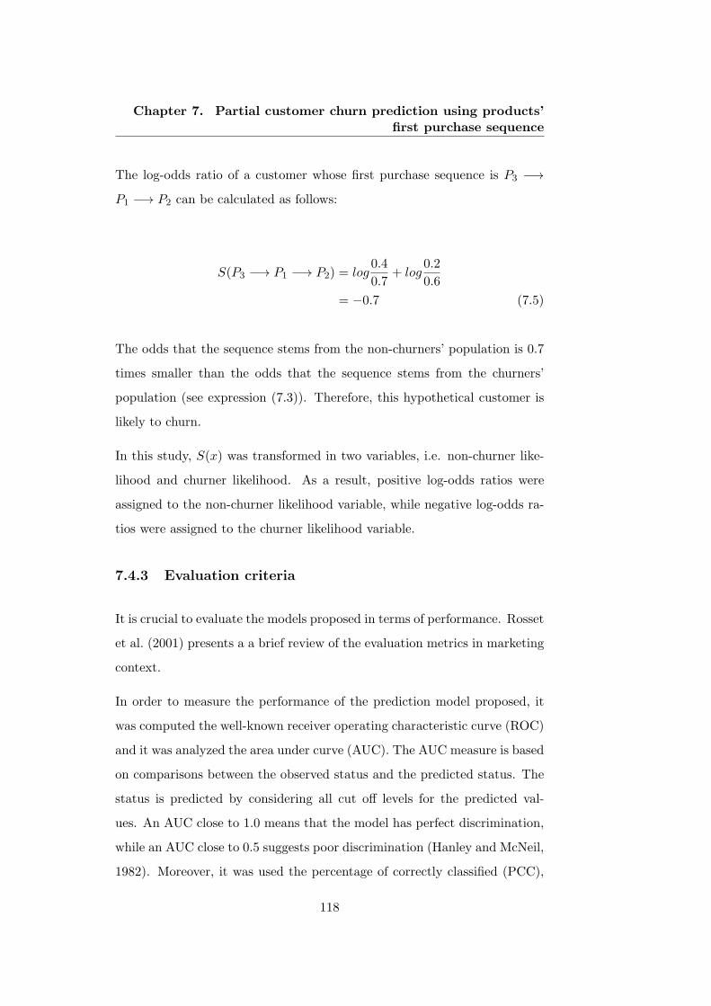
Chapter 7. Partial customer churn prediction using products’first purchase sequence
The log-odds ratio of a customer whose first purchase sequence is P3 −→
P1 −→ P2 can be calculated as follows:
S(P3 −→ P1 −→ P2) = log0.4
0.7+ log
0.2
0.6
= −0.7 (7.5)
The odds that the sequence stems from the non-churners’ population is 0.7
times smaller than the odds that the sequence stems from the churners’
population (see expression (7.3)). Therefore, this hypothetical customer is
likely to churn.
In this study, S(x) was transformed in two variables, i.e. non-churner like-
lihood and churner likelihood. As a result, positive log-odds ratios were
assigned to the non-churner likelihood variable, while negative log-odds ra-
tios were assigned to the churner likelihood variable.
7.4.3 Evaluation criteria
It is crucial to evaluate the models proposed in terms of performance. Rosset
et al. (2001) presents a a brief review of the evaluation metrics in marketing
context.
In order to measure the performance of the prediction model proposed, it
was computed the well-known receiver operating characteristic curve (ROC)
and it was analyzed the area under curve (AUC). The AUC measure is based
on comparisons between the observed status and the predicted status. The
status is predicted by considering all cut off levels for the predicted val-
ues. An AUC close to 1.0 means that the model has perfect discrimination,
while an AUC close to 0.5 suggests poor discrimination (Hanley and McNeil,
1982). Moreover, it was used the percentage of correctly classified (PCC),
118
7.5 Partial churn prediction model and retention actions
also known as accuracy, as an evaluation metric. All cases having a churn
probability above a certain threshold are classified as churners and all cases
having a below threshold churn probability are classified as non-churners.
Then, PCC is defined as the ratio between the number of correctly classified
cases and the total number of cases to be classified. According to Morrison
(1969), considering α as the actual proportion of the class to be predicted,
i.e. partial churners, PCC should exceed the proportional change criterion
defined as:
α2 + (1− α)2 (7.6)
In order to calculate the performance measures of the model proposed, the
dataset was split with 80% for training and 20% for test purposes. This sub-
division was stratified, such that the percentage of churners in both training
and test data was approximately the same as that in the initial dataset.
7.5 Partial churn prediction model and retentionactions
The analysis reported in this chapter is based on the Database 2 described
in Chapter 4. From the 95.147 new customers identified, according to the
criterion presented in Section 7.4.1 to identify partial churners, 49% partially
churned during the period of analysis, while the remaining stayed active.
For product sequence analysis, this study focused on the business unit level
of the classification of products defined by the company (see Chapter 4).
This granularity allowed the incorporation of discrimination between prod-
ucts and avoided a large degree of complexity. Moreover, only the most rep-
resentative business units concerning the purchases made by new customers,
i.e. those business units which were represented in the shopping baskets of
119
Chapter 7. Partial customer churn prediction using products’first purchase sequence
at least 10% of the new customers considered in the analysis, were selected
for the analysis. As a result, 20 business units were considered, specif-
ically grocery, hygiene/cleanliness, dairy/frozen, drinks, fruits/vegetables,
bakery, delicatessen, culture, house, meat, fish, takeaway, bricolage/auto,
leisure, storage, pets/plants, women-textile, men-textile, baby-textile and
child-textile.
The transition matrices for both the non-churner and churner populations
are shown in the Appendix. From the analysis of these matrices it is pos-
sible to conclude that most of the non-churners and churners first pur-
chase sequences include combinations between the following business units:
grocery, hygiene/cleanliness, dairy/frozen, drinks, fruits/vegetables, bakery,
delicatessen and culture. The least common transitions are those which in-
clude any business unit as an antecedent and men-textile, baby-textile and
child-textile as subsequent business units.
Both matrices exhibit different probabilities of transition between business
units. Note that the probability of buying hygiene/cleanliness products af-
ter having bought a child-textile product, and the probability of buying a
dairy/frozen product after having bought a men-textile product, are consid-
erably higher for churners than for non-churners. Moreover, the probability
of buying a product included in pet/plant business unit after having bought
a storage product is higher in the case of the non-churners than in the case
of churners.
Consider a real customer who bought Grocery in her first visit to the store,
Women-textile and Grocery in the second, Hygiene/cleanliness and Gro-
cery in the third, Fruits/vegetables, Grocery and Hygiene/cleanliness in the
fourth and, Pets/plants and House in the fifth. Therefore, the correspond-
ing sequence of the first products purchased is: Grocery −→ Women-textile
−→ Hygiene/cleanliness −→ Fruits/vegetables −→ Pets/plants and House.
120
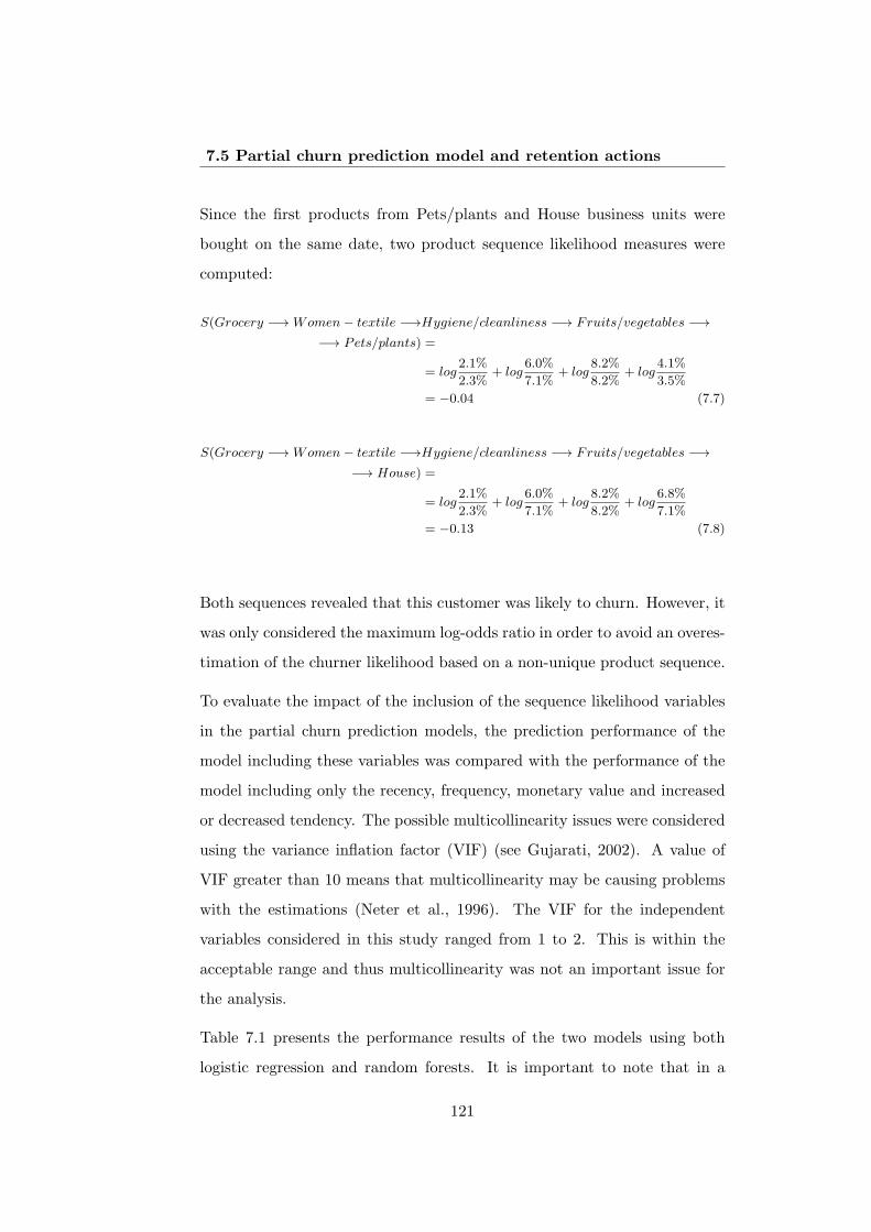
7.5 Partial churn prediction model and retention actions
Since the first products from Pets/plants and House business units were
bought on the same date, two product sequence likelihood measures were
computed:
S(Grocery −→ Women− textile −→Hygiene/cleanliness −→ Fruits/vegetables −→−→ Pets/plants) =
= log2.1%
2.3%+ log
6.0%
7.1%+ log
8.2%
8.2%+ log
4.1%
3.5%
= −0.04 (7.7)
S(Grocery −→ Women− textile −→Hygiene/cleanliness −→ Fruits/vegetables −→−→ House) =
= log2.1%
2.3%+ log
6.0%
7.1%+ log
8.2%
8.2%+ log
6.8%
7.1%
= −0.13 (7.8)
Both sequences revealed that this customer was likely to churn. However, it
was only considered the maximum log-odds ratio in order to avoid an overes-
timation of the churner likelihood based on a non-unique product sequence.
To evaluate the impact of the inclusion of the sequence likelihood variables
in the partial churn prediction models, the prediction performance of the
model including these variables was compared with the performance of the
model including only the recency, frequency, monetary value and increased
or decreased tendency. The possible multicollinearity issues were considered
using the variance inflation factor (VIF) (see Gujarati, 2002). A value of
VIF greater than 10 means that multicollinearity may be causing problems
with the estimations (Neter et al., 1996). The VIF for the independent
variables considered in this study ranged from 1 to 2. This is within the
acceptable range and thus multicollinearity was not an important issue for
the analysis.
Table 7.1 presents the performance results of the two models using both
logistic regression and random forests. It is important to note that in a
121
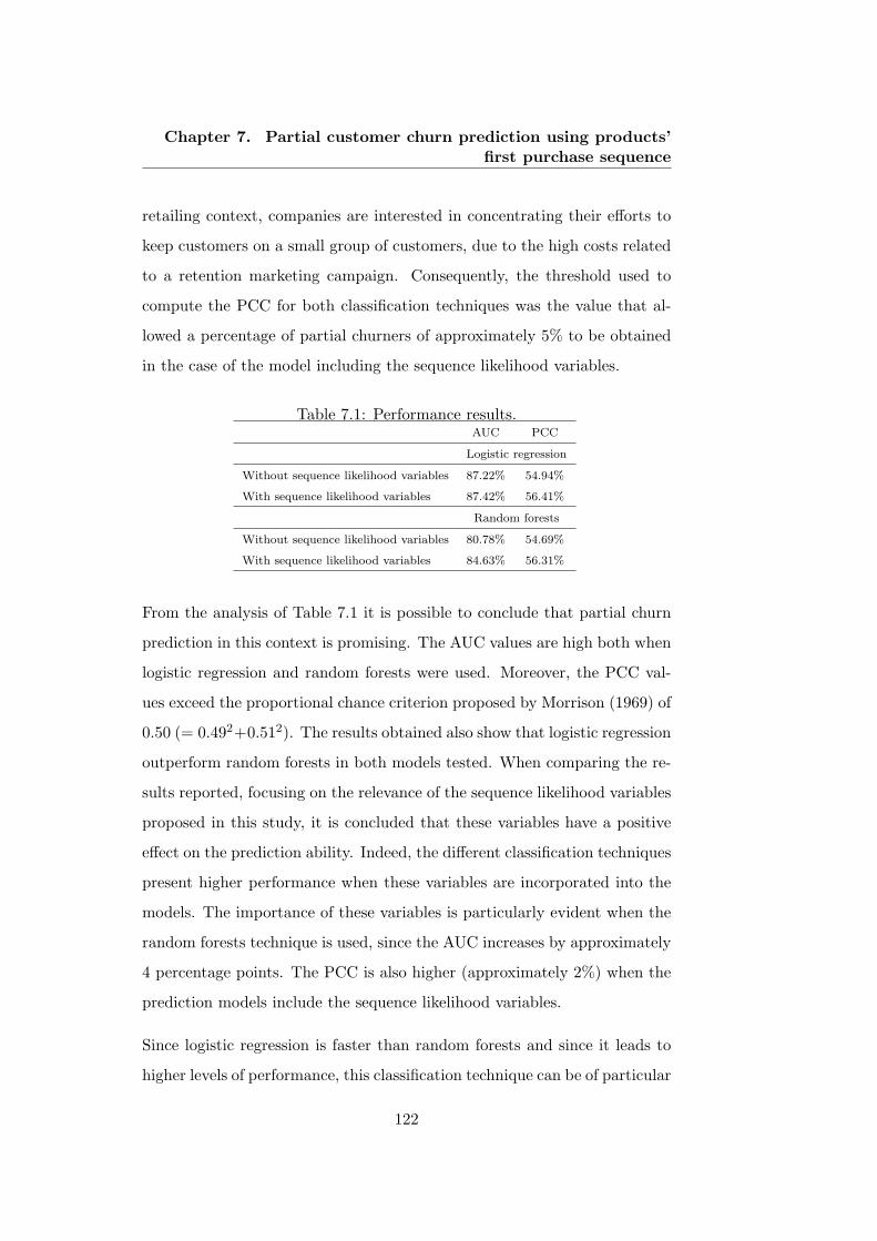
Chapter 7. Partial customer churn prediction using products’first purchase sequence
retailing context, companies are interested in concentrating their efforts to
keep customers on a small group of customers, due to the high costs related
to a retention marketing campaign. Consequently, the threshold used to
compute the PCC for both classification techniques was the value that al-
lowed a percentage of partial churners of approximately 5% to be obtained
in the case of the model including the sequence likelihood variables.
Table 7.1: Performance results.AUC PCC
Logistic regression
Without sequence likelihood variables 87.22% 54.94%
With sequence likelihood variables 87.42% 56.41%
Random forests
Without sequence likelihood variables 80.78% 54.69%
With sequence likelihood variables 84.63% 56.31%
From the analysis of Table 7.1 it is possible to conclude that partial churn
prediction in this context is promising. The AUC values are high both when
logistic regression and random forests were used. Moreover, the PCC val-
ues exceed the proportional chance criterion proposed by Morrison (1969) of
0.50 (= 0.492+0.512). The results obtained also show that logistic regression
outperform random forests in both models tested. When comparing the re-
sults reported, focusing on the relevance of the sequence likelihood variables
proposed in this study, it is concluded that these variables have a positive
effect on the prediction ability. Indeed, the different classification techniques
present higher performance when these variables are incorporated into the
models. The importance of these variables is particularly evident when the
random forests technique is used, since the AUC increases by approximately
4 percentage points. The PCC is also higher (approximately 2%) when the
prediction models include the sequence likelihood variables.
Since logistic regression is faster than random forests and since it leads to
higher levels of performance, this classification technique can be of particular
122
7.5 Partial churn prediction model and retention actions
interest for marketeers. However, it is important to note that the more
variables there are and the richer the dataset, the greater the tendency of
random forests to outperform logistic regression. In fact, even when there is
a large number of predictors, random forests do not suffer from overfitting
problems (see Breiman, 2001, for further discussion), which is not guaranteed
when using logistic regression.
The contribution of the models proposed for the company lies in the preven-
tion of wasting budget on mass marketing approaches. In fact, an accurate
churn prediction model enables the company to target the real churners, by
identifying those customers with the highest probability of churn.
Managing customer expectations to improve satisfaction is one of the best
customer retention strategies that the company can develop. Customers
have expectations concerning, for example, product quality, range of prod-
ucts, service responsiveness, price stability, promotional activity and staff
empathy. Therefore, it seems of utmost importance for the company to
clearly know the expectations of the potential churners, by means of an in-
dividual contact. This can support the design of a effective differentiated
service which may ensure the long term relationship of the customers with
the company.
Moreover, other retention strategies, not directly related to customer ex-
pectations, can be undertaken. For instance, to be sure to stay in touch
with the potential churners by placing phone calls or send emails, special of-
fers, customized advertising, follow-ups, and cards or notes with a personal
touch. The company can also consider to send good deals to the potential
churners identified by the models. These might be, for instance, discounts
on the purchases and an extra gift included with a purchase. Customers
usually answer to these actions positively, as they feel valued and important
for the company.
123
Chapter 7. Partial customer churn prediction using products’first purchase sequence
7.6 Conclusion
This study proposed a model to predict partial customer churn in the retail
sector. This model contributes to the literature by including a measure of
the similarity of the sequence of customers’ first purchases, in terms of prod-
uct business unit, with the sequence recorded for churners and non-churners.
This sequence likelihood was modeled using markov-for-discrimination. Both
logistic regression and random forests were used in this study.
The results reported highlighted the relevance of the model proposed, since
the performance of the model including the sequence likelihood variables
was higher than the performance of the model not including these variables.
This supremacy was measured in terms of the area under the receiver op-
erating characteristic curve and percentage of correctly classified instances.
Furthermore, the results reported suggested that the logistic regression tech-
nique outperforms the random forests technique.
By using the prediction model proposed in this chapter, companies can tar-
get possible future churners in retention marketing campaigns. For example,
the model can help companies to decide whether or not to send a promo-
tional voucher to a customer.
124
Chapter 8
Partial customer churnprediction using variablelength products’ firstpurchase sequences
8.1 Introduction
This chapter revisits the customer retention topic and develops another
churn prediction model. This study aims at exploring different forms of
including the sequences of the first products purchased. It is intended to
include in the prediction models variable length sequences. Moreover, the
sequences of the first products purchased are modeled in chronological order
as well as in reverse chronological order. The classification technique used
in this study is logistic regression.
The content of the remainder of this chapter is as follows. Section 8.2
introduces the motivation for the inclusion of variable length sequences of
the first products purchased in the churn prediction model. Section 8.3
introduces the methodology followed in this study, namely the predictors
proposed and the performance evaluation criteria used. Section 8.4 presents
125
Chapter 8. Partial customer churn prediction using variablelength products’ first purchase sequences
the application and discusses the results obtained. Section 8.5 presents the
main conclusions.
8.2 Variable length sequences
Similarly to what was done in Chapter 7, it is assumed that the sequences
of the first products purchased may reveal the state of trust of a customer
towards a company. Some authors claim that the beginning of the rela-
tionship between customers and companies is critical for the development
of a long term relationship (Lawson-Body and Limayem, 2004), while oth-
ers claim that the course of the relationship replaces the initial impressions
(Redondo and Fierro, 2005). Thus, this study analyzes both the churn pre-
diction power derived from the sequence of the first products’ business unit
purchased in chronological order and in reverse chronological order.
For each sequence of the first products purchased, according to the specific
purchase process, the period of definition of a first impression can be differ-
ent. Moreover, the relevant history of first products’ business unit purchases
can be distinct. Therefore, it is considered in both forward and backward
analysis sequences of variable length. Indeed, it is used the idea underly-
ing the variable memory concept, introduced by Rissanen (1983) in variable
length markov chains (VLMC) context, to incorporate in the model proposed
adjusted sequences of the first products purchased. Sequences of different
length are included in the models, based on the discrimination power of the
sequences considered.
8.3 Methodology
This study aims to predict partial churn by considering variable length se-
quences of the first products purchased, depending on whether a longer first
126
8.3 Methodology
sequence contributes to a more accurate model. Two distinct models were
run: one in which the sequences were included in chronological order (for-
ward model) and another in which the sequences were included in reverse
chronological order (backward model).
The relevance of the two models proposed was measured by comparing their
performance with performance of the standard RFM model. Since the meth-
odology proposed involved running several models, the logistic regression
was selected as the classification technique. It is fast and enables to obtain
robust results. The criterion used to infer partial attrition was the same
used in the previous chapter, as well as the data.
In the next sections the evaluation criteria used to compare models’ perfor-
mance and the innovative explanatory variables included in the models are
presented.
8.3.1 Evaluation criteria
The AUC was computed to measure the performance of the binary prediction
models. Moreover, lift was also used as evaluation metric. This measure
focuses on the segment of customers with the highest risk to the company,
i.e. customers with the highest probability to churn. The definition of lift
depends on the percentage of customers the company intends to achieve on
a retention campaign. Consider that a company is interested in the top p-
th percentile of most likely churners, based on predicted churn probabilities.
The top p-th percentile lift then equals the ratio of the proportion of churners
in the top p-th percentile of ordered posterior churn probabilities to the
churn rate in the total customer population. For example, a p-th percentile
lift of 3 means that the model under investigation identifies three times
more churners in the top p% than a random assignment would do. Since
the proportion of customers that a company is able and willing to target
127
Chapter 8. Partial customer churn prediction using variablelength products’ first purchase sequences
depends on the specific context, namely the available budget, this study
included the lift performance for different percentiles (1%, 5%, 10%).
The performance measures were again computed by splitting the dataset in
80% for training and 20% for test purposes. This subdivision was stratified,
such that the percentage of churners in both training and test data was
approximately identical to the values corresponding to the initial dataset.
8.3.2 Explanatory variables
This study explored the potential of past behavior variables to distinguish
churners from non-churners. In both churn models the recency, frequency
and monetary variables, already presented in Chapter 7 were included.
Moreover, it was included in the forward and in the backward models a
set of variables that indicated whether or not a specific sequence of prod-
ucts’ business unit was observed on the past transactional behavior of the
customer.
Both forward sequences and backward sequences were included in the dif-
ferent models by means of a set of dummy variables. In the forward model,
each forward sequence dummy variable represented a sequence of the first
products’ business unit purchased in chronological order, i.e. the first busi-
ness unit bought was at the bottom and the most recent was on top. In
the backward model, each backward sequence dummy variable represented
a sequence of the first products’ business unit purchased in reverse chrono-
logical order, i.e. the products’ business unit bought most recently was in
the bottom and the oldest one on top.
The selection of the dummy variables for the two models followed a similar
procedure. In the first stage, the dummy variables representing all sub-
sequences of length two, i.e. the first products’ business unit bought and
the second products’ business unit bought, in the case of the forward model,
128
8.4 Partial churn prediction model
and, the last products’ business unit bought and the second last products’
business unit bought, in the case of the backward model were computed.
Then, for those sequences of length two, which were observed for more than
500 customers, the corresponding sequences of length three were computed,
and so on. It was assumed that this first selection process based on the fre-
quency enabled to exclude from the posterior analysis sequences that would
not contribute to the discrimination between churners and non-churners. In
the second stage, all dummy variables resulting from the first selection were
used to conduct an in-depth logistic regression analysis. It means that it
was run a logistic model including each dummy variable corresponding to
the sequence of length two and the RFM variables. For those sequences that
resulted in an increase of the AUC, in relation to the AUC observed for the
RFM model, this study went deeper, i.e. it was run a logistic regression
with each dummy variable corresponding to the sequence of length three.
This procedure was progressively executed and stopped when the AUC did
not increase. In the third stage, having identified the dummy variables
which individually allowed to increase the prediction performance in terms
of AUC, it was conducted a multiple logistic regression which included all
these variables.
8.4 Partial churn prediction model
The analysis reported in this chapter was also based on the new customers
included in the Database 2, described in Chapter 4. The criteria used to
identify the new customers were the same introduced in Chapter 7.
By applying the forward churn prediction analysis proposed, in the first
stage, 6968 forward sequences were identified. These sequences were consid-
ered relevant in terms of frequency. As shown in Table 8.1, 380 sequences of
length two were analyzed, i.e. combinations of two out of 20 product business
129
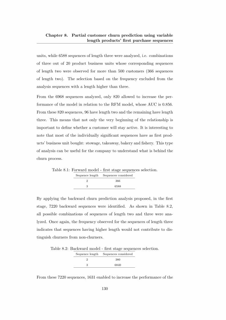
Chapter 8. Partial customer churn prediction using variablelength products’ first purchase sequences
units, while 6588 sequences of length three were analyzed, i.e. combinations
of three out of 20 product business units whose corresponding sequences
of length two were observed for more than 500 customers (366 sequences
of length two). The selection based on the frequency excluded from the
analysis sequences with a length higher than three.
From the 6968 sequences analyzed, only 820 allowed to increase the per-
formance of the model in relation to the RFM model, whose AUC is 0.856.
From these 820 sequences, 96 have length two and the remaining have length
three. This means that not only the very beginning of the relationship is
important to define whether a customer will stay active. It is interesting to
note that most of the individually significant sequences have as first prod-
ucts’ business unit bought: stowage, takeaway, bakery and fishery. This type
of analysis can be useful for the company to understand what is behind the
churn process.
Table 8.1: Forward model - first stage sequences selection.Sequence length Sequences considered
2 366
3 6588
By applying the backward churn prediction analysis proposed, in the first
stage, 7220 backward sequences were identified. As shown in Table 8.2,
all possible combinations of sequences of length two and three were ana-
lyzed. Once again, the frequency observed for the sequences of length three
indicates that sequences having higher length would not contribute to dis-
tinguish churners from non-churners.
Table 8.2: Backward model - first stage sequences selection.Sequence length Sequences considered
2 380
3 6840
From these 7220 sequences, 1631 enabled to increase the performance of the
130
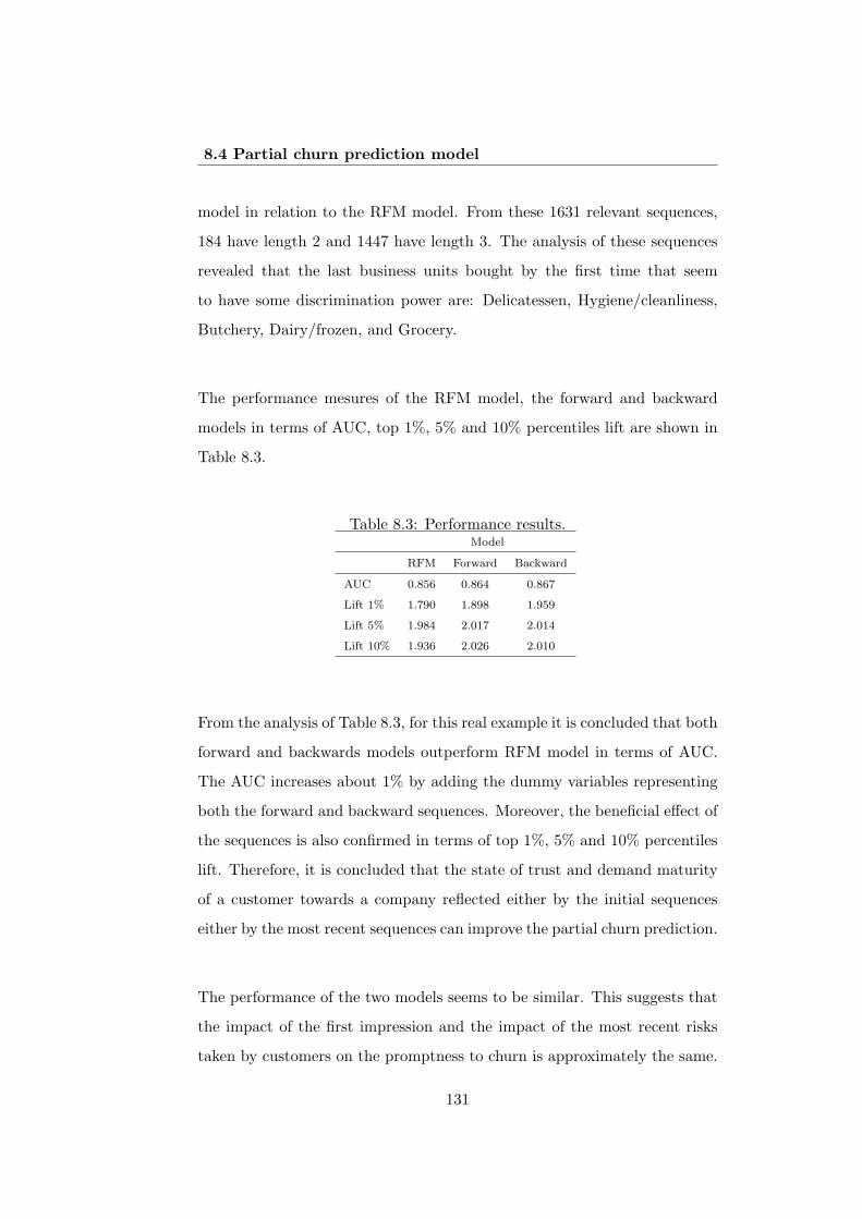
8.4 Partial churn prediction model
model in relation to the RFM model. From these 1631 relevant sequences,
184 have length 2 and 1447 have length 3. The analysis of these sequences
revealed that the last business units bought by the first time that seem
to have some discrimination power are: Delicatessen, Hygiene/cleanliness,
Butchery, Dairy/frozen, and Grocery.
The performance mesures of the RFM model, the forward and backward
models in terms of AUC, top 1%, 5% and 10% percentiles lift are shown in
Table 8.3.
Table 8.3: Performance results.Model
RFM Forward Backward
AUC 0.856 0.864 0.867
Lift 1% 1.790 1.898 1.959
Lift 5% 1.984 2.017 2.014
Lift 10% 1.936 2.026 2.010
From the analysis of Table 8.3, for this real example it is concluded that both
forward and backwards models outperform RFM model in terms of AUC.
The AUC increases about 1% by adding the dummy variables representing
both the forward and backward sequences. Moreover, the beneficial effect of
the sequences is also confirmed in terms of top 1%, 5% and 10% percentiles
lift. Therefore, it is concluded that the state of trust and demand maturity
of a customer towards a company reflected either by the initial sequences
either by the most recent sequences can improve the partial churn prediction.
The performance of the two models seems to be similar. This suggests that
the impact of the first impression and the impact of the most recent risks
taken by customers on the promptness to churn is approximately the same.
131
Chapter 8. Partial customer churn prediction using variablelength products’ first purchase sequences
8.5 Conclusion
In this study, it was proposed two predictive models for partial customer
churn in the retail sector. Both models included the sequence of the first
products’ business unit purchased as a proxy of the state of trust and de-
mand maturity of customers towards a company. Considering the impact
of the first impression on the current state of the relationship as well as the
impact of the most recent risks undertaken, it was modeled the first pur-
chase sequence in chronological order as well as in reverse order, respectively.
Both sequences of first products purchased were modeled by considering a
variable length, defined according to the models’ accuracy.
The results of the application revealed that both models proposed outper-
formed the standard RFM model, which highlighted the relevance of the
state of trust and demand maturity in the partial churn prediction. The
models’ performance was measured in terms of AUC and p-th percentile
lift.
132

Chapter 9
Conclusions
9.1 Introduction
This chapter presents a summary of the research conducted, as well as the
conclusions drawn. It also identifies the main contributions of the thesis to
the marketing modeling literature. Finally it presents some directions for
future research.
9.2 Summary and conclusions
From the analysis of the evolution of the retail sector, it is concluded that the
reinforcement of relationship marketing is of utmost importance in today’s
context of thriving competition. The development of methodologies to sup-
port customer relationship management in retailing can increase companies’
volume of sales.
Following this idea, this thesis started by introducing the main concepts
concerning marketing and customer relationship management. Currently,
marketing is focused on establishing, maintaining and enhancing relation-
ships with customers. Customer relationship management is a technological
133
Chapter 9. Conclusions
manifestation of relationship marketing and can be defined as the process of
handling customer relationships in practice. CRM integrates mainly three
components: operational, collaborative and analytical CRM. Four main re-
search directions concerning analytical CRM were identified: customer iden-
tification, customer attraction, customer development and customer reten-
tion. Moreover, by revising some research on CRM field, it was concluded
that the study of each one of these dimensions in the retail sector is still
incipient, enabling room for improvement.
Considering this research opportunity, this thesis is focused on analytical
customer relationship management. Thus, it was presented the knowledge
discovery in databases process, which consists of data selection, data prepro-
cessing, data transformation, data mining and interpretation or evaluation.
It was given emphasis to data mining, i.e. the process of extracting or detect-
ing hidden patterns or information in large databases. This doctoral thesis
described the main data mining tools: association, classification, clustering,
forecasting, regression, sequence discovery and visualization. From these
tools, clustering, classification and association are the ones more frequently
used to support customer relationship management. For customer identifica-
tion purposes, classification and clustering techniques are those mainly used.
For customers’ attraction, classification models are the most frequently used.
For retention purposes, association and classification are the most frequently
used. Concerning customers’ development, association models are the most
frequent. For each distinct data mining tool, this thesis presented the most
popular techniques and corresponding advantages and disadvantages. It was
concluded that there is no consensus regarding the most suitable techniques
to use. However, in many cases, processing speed is one of the criteria that
justifies the choice of a specific technique.
The main objective of the research was to develop a methodology to support
customer relationship management in the retail sector, such that the rela-
134
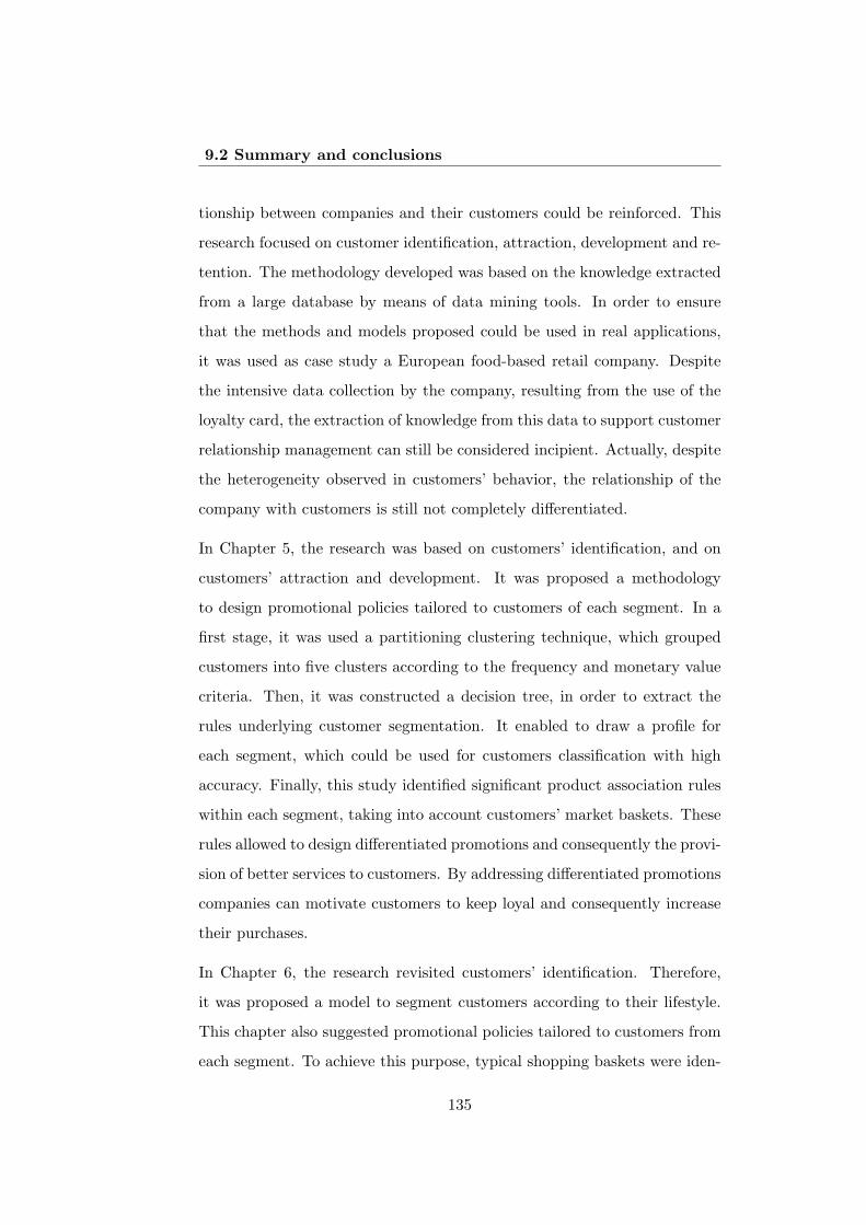
9.2 Summary and conclusions
tionship between companies and their customers could be reinforced. This
research focused on customer identification, attraction, development and re-
tention. The methodology developed was based on the knowledge extracted
from a large database by means of data mining tools. In order to ensure
that the methods and models proposed could be used in real applications,
it was used as case study a European food-based retail company. Despite
the intensive data collection by the company, resulting from the use of the
loyalty card, the extraction of knowledge from this data to support customer
relationship management can still be considered incipient. Actually, despite
the heterogeneity observed in customers’ behavior, the relationship of the
company with customers is still not completely differentiated.
In Chapter 5, the research was based on customers’ identification, and on
customers’ attraction and development. It was proposed a methodology
to design promotional policies tailored to customers of each segment. In a
first stage, it was used a partitioning clustering technique, which grouped
customers into five clusters according to the frequency and monetary value
criteria. Then, it was constructed a decision tree, in order to extract the
rules underlying customer segmentation. It enabled to draw a profile for
each segment, which could be used for customers classification with high
accuracy. Finally, this study identified significant product association rules
within each segment, taking into account customers’ market baskets. These
rules allowed to design differentiated promotions and consequently the provi-
sion of better services to customers. By addressing differentiated promotions
companies can motivate customers to keep loyal and consequently increase
their purchases.
In Chapter 6, the research revisited customers’ identification. Therefore,
it was proposed a model to segment customers according to their lifestyle.
This chapter also suggested promotional policies tailored to customers from
each segment. To achieve this purpose, typical shopping baskets were iden-
135
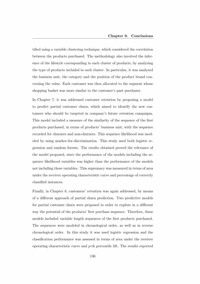
Chapter 9. Conclusions
tified using a variable clustering technique, which considered the correlation
between the products purchased. The methodology also involved the infer-
ence of the lifestyle corresponding to each cluster of products, by analyzing
the type of products included in each cluster. In particular, it was analyzed
the business unit, the category and the position of the product brand con-
cerning the value. Each customer was then allocated to the segment whose
shopping basket was more similar to the customer’s past purchases.
In Chapter 7, it was addressed customer retention by proposing a model
to predict partial customer churn, which aimed to identify the new cus-
tomers who should be targeted in company’s future retention campaigns.
This model included a measure of the similarity of the sequence of the first
products purchased, in terms of products’ business unit, with the sequence
recorded for churners and non-churners. This sequence likelihood was mod-
eled by using markov-for-discrimination. This study used both logistic re-
gression and random forests. The results obtained proved the relevance of
the model proposed, since the performance of the models including the se-
quence likelihood variables was higher than the performance of the models
not including these variables. This supremacy was measured in terms of area
under the receiver operating characteristic curve and percentage of correctly
classified instances.
Finally, in Chapter 8, customers’ retention was again addressed, by means
of a different approach of partial churn prediction. Two predictive models
for partial customer churn were proposed in order to explore in a different
way the potential of the products’ first purchase sequence. Therefore, these
models included variable length sequences of the first products purchased.
The sequences were modeled in chronological order, as well as in reverse
chronological order. In this study it was used logistic regression and the
classification performance was assessed in terms of area under the receiver
operating characteristic curve and p-th percentile lift. The results reported
136
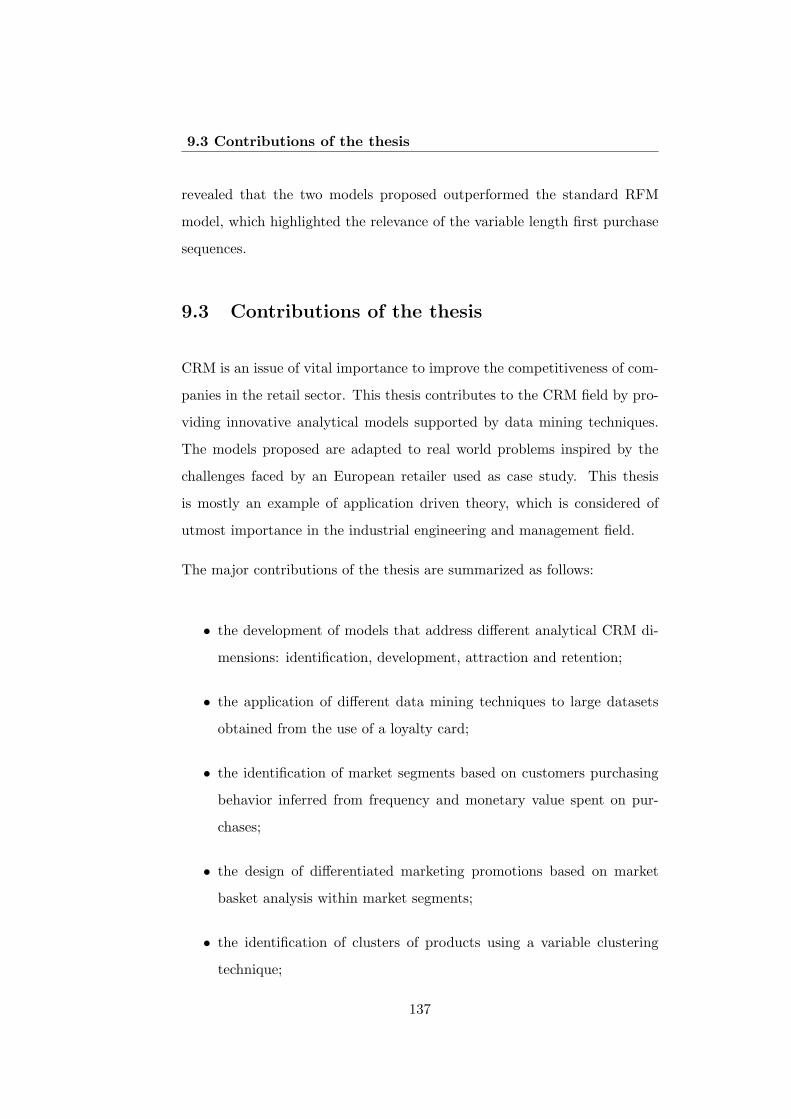
9.3 Contributions of the thesis
revealed that the two models proposed outperformed the standard RFM
model, which highlighted the relevance of the variable length first purchase
sequences.
9.3 Contributions of the thesis
CRM is an issue of vital importance to improve the competitiveness of com-
panies in the retail sector. This thesis contributes to the CRM field by pro-
viding innovative analytical models supported by data mining techniques.
The models proposed are adapted to real world problems inspired by the
challenges faced by an European retailer used as case study. This thesis
is mostly an example of application driven theory, which is considered of
utmost importance in the industrial engineering and management field.
The major contributions of the thesis are summarized as follows:
• the development of models that address different analytical CRM di-
mensions: identification, development, attraction and retention;
• the application of different data mining techniques to large datasets
obtained from the use of a loyalty card;
• the identification of market segments based on customers purchasing
behavior inferred from frequency and monetary value spent on pur-
chases;
• the design of differentiated marketing promotions based on market
basket analysis within market segments;
• the identification of clusters of products using a variable clustering
technique;
137
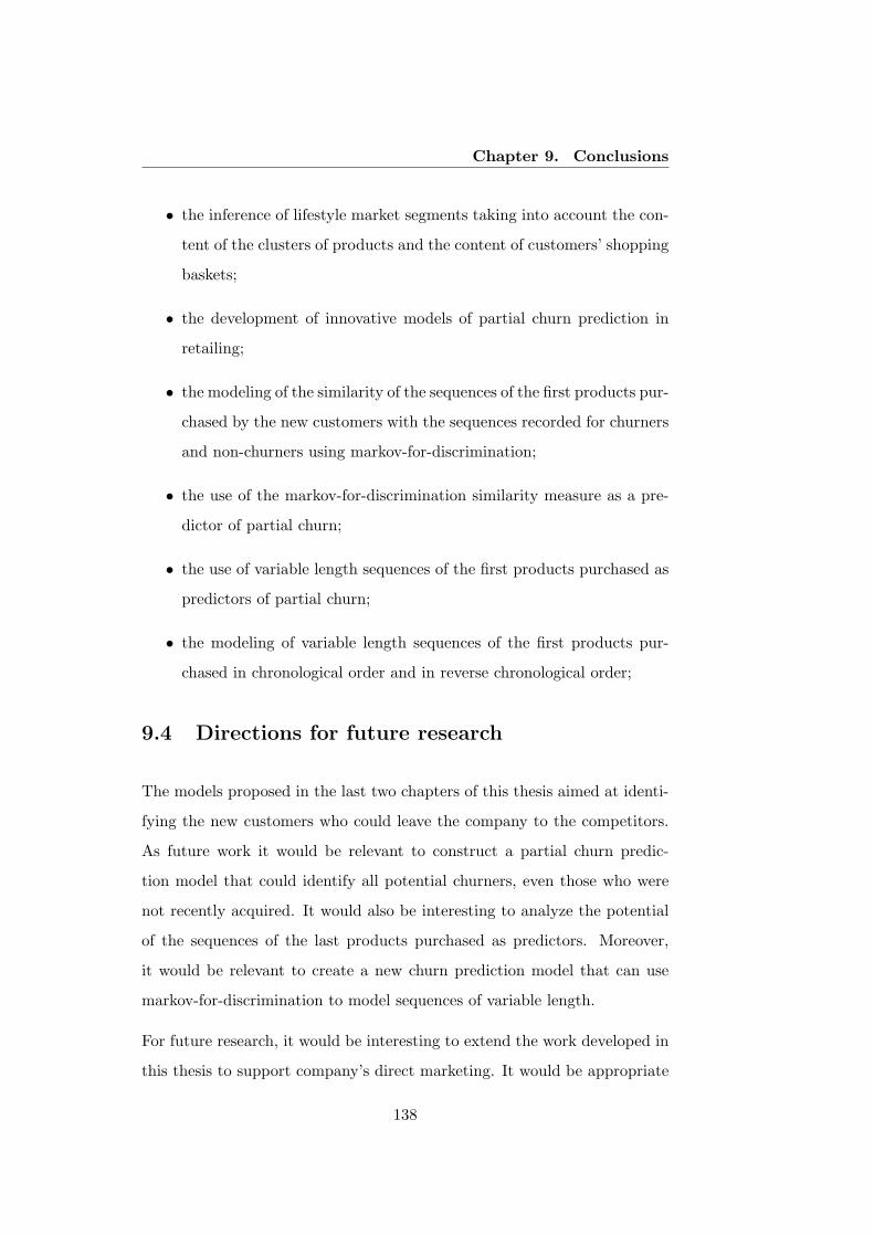
Chapter 9. Conclusions
• the inference of lifestyle market segments taking into account the con-
tent of the clusters of products and the content of customers’ shopping
baskets;
• the development of innovative models of partial churn prediction in
retailing;
• the modeling of the similarity of the sequences of the first products pur-
chased by the new customers with the sequences recorded for churners
and non-churners using markov-for-discrimination;
• the use of the markov-for-discrimination similarity measure as a pre-
dictor of partial churn;
• the use of variable length sequences of the first products purchased as
predictors of partial churn;
• the modeling of variable length sequences of the first products pur-
chased in chronological order and in reverse chronological order;
9.4 Directions for future research
The models proposed in the last two chapters of this thesis aimed at identi-
fying the new customers who could leave the company to the competitors.
As future work it would be relevant to construct a partial churn predic-
tion model that could identify all potential churners, even those who were
not recently acquired. It would also be interesting to analyze the potential
of the sequences of the last products purchased as predictors. Moreover,
it would be relevant to create a new churn prediction model that can use
markov-for-discrimination to model sequences of variable length.
For future research, it would be interesting to extend the work developed in
this thesis to support company’s direct marketing. It would be appropriate
138
9.4 Directions for future research
to develop a model to predict customers response to direct marketing cam-
paigns. The use of classification techniques based on bagging and boosting
methods would be interesting.
A relevant topic would also be the development of a model to monitor the
relationship between the customers and the company, taking into account
the response of customers to past direct marketing campaigns. This model
would enable the company to typify customers according to their response
to different kinds of marketing actions. Thus, the company would be able
to efficiently target its marketing actions.
As future work it would also be interesting to construct a model to assess
customers lifetime value, in order to rank company’s customers and conse-
quently adjust the target of company’s actions. It would also be relevant
to verify the impact of customers response to direct marketing actions on
customers lifetime value.
The methodologies proposed can be adjusted and applied to other business
contexts, in which customer relationship management is also crucial to guar-
antee companies’ competitiveness. Fields that could be studied in the future
cover for example banking, insurance and telecommunications.
139

Chapter 9. Conclusions
140

Appendix A
Appendix
141
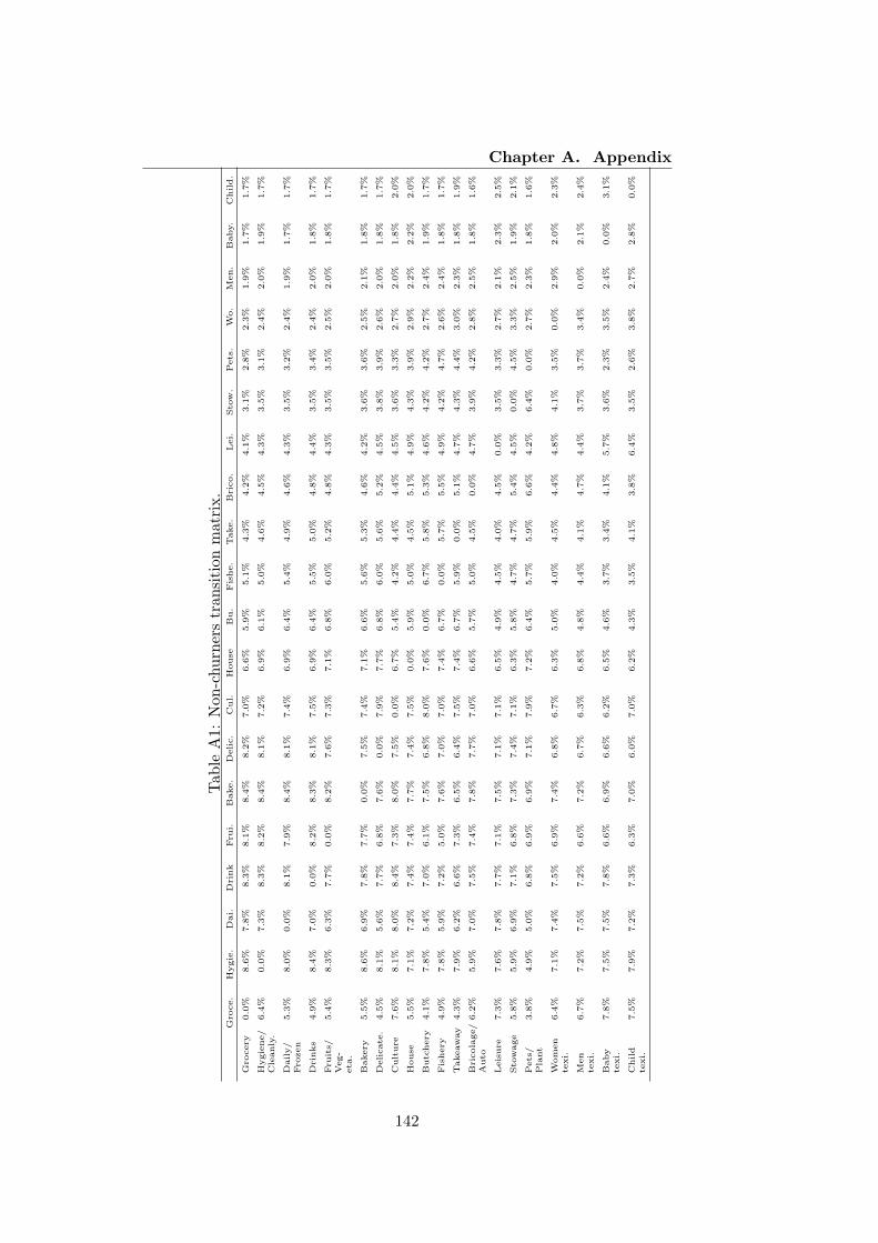
Chapter A. Appendix
Tab
leA1:Non-churnerstransitionmatrix.
Gro
ce.
Hygie.
Dai.
Drink
Fru
i.Bake.
Delic.
Cul.
House
Bu.
Fishe.
Take.
Brico.
Lei.
Sto
w.
Pets.
Wo.
Men.
Baby.
Child.
Gro
cery
0.0%
8.6%
7.8%
8.3%
8.1%
8.4%
8.2%
7.0%
6.6%
5.9%
5.1%
4.3%
4.2%
4.1%
3.1%
2.8%
2.3%
1.9%
1.7%
1.7%
Hygiene/
Cleanly.
6.4%
0.0%
7.3%
8.3%
8.2%
8.4%
8.1%
7.2%
6.9%
6.1%
5.0%
4.6%
4.5%
4.3%
3.5%
3.1%
2.4%
2.0%
1.9%
1.7%
Daily/
Fro
zen
5.3%
8.0%
0.0%
8.1%
7.9%
8.4%
8.1%
7.4%
6.9%
6.4%
5.4%
4.9%
4.6%
4.3%
3.5%
3.2%
2.4%
1.9%
1.7%
1.7%
Drinks
4.9%
8.4%
7.0%
0.0%
8.2%
8.3%
8.1%
7.5%
6.9%
6.4%
5.5%
5.0%
4.8%
4.4%
3.5%
3.4%
2.4%
2.0%
1.8%
1.7%
Fru
its/
Veg-
eta
.
5.4%
8.3%
6.3%
7.7%
0.0%
8.2%
7.6%
7.3%
7.1%
6.8%
6.0%
5.2%
4.8%
4.3%
3.5%
3.5%
2.5%
2.0%
1.8%
1.7%
Bakery
5.5%
8.6%
6.9%
7.8%
7.7%
0.0%
7.5%
7.4%
7.1%
6.6%
5.6%
5.3%
4.6%
4.2%
3.6%
3.6%
2.5%
2.1%
1.8%
1.7%
Delicate
.4.5%
8.1%
5.6%
7.7%
6.8%
7.6%
0.0%
7.9%
7.7%
6.8%
6.0%
5.6%
5.2%
4.5%
3.8%
3.9%
2.6%
2.0%
1.8%
1.7%
Culture
7.6%
8.1%
8.0%
8.4%
7.3%
8.0%
7.5%
0.0%
6.7%
5.4%
4.2%
4.4%
4.4%
4.5%
3.6%
3.3%
2.7%
2.0%
1.8%
2.0%
House
5.5%
7.1%
7.2%
7.4%
7.4%
7.7%
7.4%
7.5%
0.0%
5.9%
5.0%
4.5%
5.1%
4.9%
4.3%
3.9%
2.9%
2.2%
2.2%
2.0%
Butchery
4.1%
7.8%
5.4%
7.0%
6.1%
7.5%
6.8%
8.0%
7.6%
0.0%
6.7%
5.8%
5.3%
4.6%
4.2%
4.2%
2.7%
2.4%
1.9%
1.7%
Fishery
4.9%
7.8%
5.9%
7.2%
5.0%
7.6%
7.0%
7.0%
7.4%
6.7%
0.0%
5.7%
5.5%
4.9%
4.2%
4.7%
2.6%
2.4%
1.8%
1.7%
Takeaway
4.3%
7.9%
6.2%
6.6%
7.3%
6.5%
6.4%
7.5%
7.4%
6.7%
5.9%
0.0%
5.1%
4.7%
4.3%
4.4%
3.0%
2.3%
1.8%
1.9%
Bricolage/
Auto
6.2%
5.9%
7.0%
7.5%
7.4%
7.8%
7.7%
7.0%
6.6%
5.7%
5.0%
4.5%
0.0%
4.7%
3.9%
4.2%
2.8%
2.5%
1.8%
1.6%
Leisure
7.3%
7.6%
7.8%
7.7%
7.1%
7.5%
7.1%
7.1%
6.5%
4.9%
4.5%
4.0%
4.5%
0.0%
3.5%
3.3%
2.7%
2.1%
2.3%
2.5%
Sto
wage
5.8%
5.9%
6.9%
7.1%
6.8%
7.3%
7.4%
7.1%
6.3%
5.8%
4.7%
4.7%
5.4%
4.5%
0.0%
4.5%
3.3%
2.5%
1.9%
2.1%
Pets/
Plant
3.8%
4.9%
5.0%
6.8%
6.9%
6.9%
7.1%
7.9%
7.2%
6.4%
5.7%
5.9%
6.6%
4.2%
6.4%
0.0%
2.7%
2.3%
1.8%
1.6%
Women
texi.
6.4%
7.1%
7.4%
7.5%
6.9%
7.4%
6.8%
6.7%
6.3%
5.0%
4.0%
4.5%
4.4%
4.8%
4.1%
3.5%
0.0%
2.9%
2.0%
2.3%
Men
texi.
6.7%
7.2%
7.5%
7.2%
6.6%
7.2%
6.7%
6.3%
6.8%
4.8%
4.4%
4.1%
4.7%
4.4%
3.7%
3.7%
3.4%
0.0%
2.1%
2.4%
Baby
texi.
7.8%
7.5%
7.5%
7.8%
6.6%
6.9%
6.6%
6.2%
6.5%
4.6%
3.7%
3.4%
4.1%
5.7%
3.6%
2.3%
3.5%
2.4%
0.0%
3.1%
Child
texi.
7.5%
7.9%
7.2%
7.3%
6.3%
7.0%
6.0%
7.0%
6.2%
4.3%
3.5%
4.1%
3.8%
6.4%
3.5%
2.6%
3.8%
2.7%
2.8%
0.0%
142
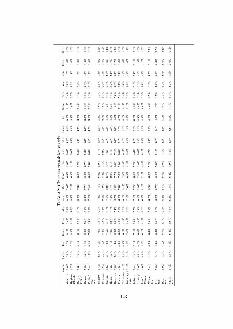
Tab
leA2:Churnerstransitionmatrix.
Gro
ce.
Hygie.
Dai.
Drink
Fru
i.Bake.
Delic.
Cul.
House
Bu.
Fishe.
Take.
Brico.
Lei.
Sto
w.
Pets.
Wo.
Men.
Baby.
Child.
Gro
cery
0.0%
8.7%
7.6%
8.1%
8.0%
8.7%
8.5%
7.0%
6.4%
6.3%
5.0%
4.7%
4.3%
3.3%
3.2%
3.4%
2.1%
1.7%
1.6%
1.6%
Hygiene/
Cleanly.
6.7%
0.0%
7.5%
8.2%
8.2%
8.7%
8.4%
7.2%
6.9%
6.1%
5.0%
4.8%
4.6%
3.4%
3.6%
3.7%
2.3%
1.8%
1.6%
1.6%
Daily/
Fro
zen
5.6%
8.2%
0.0%
8.1%
7.9%
8.6%
8.3%
7.3%
6.8%
6.7%
5.4%
5.1%
4.5%
3.3%
3.4%
3.8%
2.2%
1.7%
1.6%
1.6%
Drinks
5.0%
8.2%
6.6%
0.0%
7.8%
8.2%
8.2%
7.7%
6.9%
6.7%
5.3%
5.4%
4.9%
3.5%
3.8%
4.1%
2.4%
1.9%
1.6%
1.6%
Fru
its/
Veg-
eta
.
5.4%
8.1%
6.2%
7.8%
0.0%
8.4%
7.8%
7.4%
6.8%
7.0%
6.0%
5.2%
4.9%
3.5%
3.9%
4.1%
2.3%
1.9%
1.5%
1.6%
Bakery
5.4%
8.5%
6.9%
7.6%
7.5%
0.0%
7.8%
7.4%
6.9%
6.9%
5.7%
5.7%
5.0%
3.5%
4.0%
4.0%
2.3%
1.8%
1.6%
1.6%
Delicate
.4.6%
8.0%
5.5%
7.4%
7.0%
7.4%
0.0%
7.9%
7.3%
7.4%
6.2%
6.0%
5.5%
3.7%
4.2%
4.4%
2.5%
1.9%
1.6%
1.5%
Culture
6.6%
7.5%
7.4%
7.5%
7.1%
8.0%
7.6%
0.0%
6.7%
5.7%
4.6%
5.3%
5.0%
4.0%
4.3%
4.3%
2.8%
2.1%
1.6%
2.1%
House
5.3%
6.2%
6.5%
7.2%
6.9%
7.5%
7.2%
7.7%
0.0%
6.1%
5.1%
5.3%
5.3%
4.1%
5.3%
4.9%
3.2%
2.4%
1.7%
2.0%
Butchery
3.8%
7.4%
5.1%
6.9%
6.0%
7.1%
6.7%
8.0%
7.7%
0.0%
7.1%
6.2%
5.6%
4.1%
4.8%
5.2%
2.6%
2.3%
1.7%
1.7%
Fishery
4.5%
6.8%
5.1%
6.6%
4.5%
7.2%
6.5%
7.8%
7.8%
7.5%
0.0%
6.0%
6.1%
4.7%
5.1%
5.2%
2.7%
2.4%
1.8%
1.6%
Takeaway
4.1%
7.4%
5.4%
6.2%
6.9%
6.0%
6.2%
8.1%
7.5%
6.9%
6.2%
0.0%
5.7%
4.2%
5.1%
5.4%
3.1%
2.3%
1.6%
1.8%
Bricolage/
auto
5.2%
5.4%
5.9%
7.0%
6.9%
7.4%
7.1%
7.6%
6.9%
6.2%
5.4%
5.4%
0.0%
4.3%
5.2%
5.3%
2.7%
2.3%
1.6%
1.8%
Leisure
6.4%
6.4%
7.0%
7.1%
6.6%
7.5%
7.1%
7.2%
6.5%
5.2%
4.6%
4.3%
5.1%
0.0%
4.3%
4.4%
3.0%
2.4%
2.1%
2.8%
Sto
wage
5.0%
4.7%
5.8%
6.0%
6.4%
6.7%
6.8%
7.3%
7.0%
5.8%
5.6%
6.1%
5.9%
4.4%
0.0%
6.1%
3.6%
2.8%
1.9%
1.9%
Pets/
Plants
4.0%
4.8%
5.4%
6.1%
6.3%
6.5%
6.6%
8.1%
7.1%
6.4%
6.1%
6.1%
6.5%
4.2%
6.6%
0.0%
3.1%
2.6%
1.7%
1.9%
Women
texi.
5.4%
6.0%
6.7%
6.4%
6.6%
7.2%
6.7%
6.9%
6.6%
5.2%
4.7%
5.1%
5.0%
4.5%
4.6%
4.5%
0.0%
3.2%
2.1%
2.7%
Men
texi.
5.8%
6.4%
6.1%
6.3%
6.2%
6.8%
6.0%
6.7%
6.6%
5.3%
5.1%
4.6%
5.4%
4.3%
4.7%
4.7%
4.2%
0.0%
2.3%
2.5%
Baby
texi.
6.9%
7.0%
7.2%
6.7%
6.4%
6.6%
6.3%
6.5%
6.7%
5.0%
4.1%
4.3%
4.3%
5.5%
4.0%
3.0%
3.8%
2.7%
0.0%
3.1%
Child
texi.
6.4%
6.3%
6.5%
6.4%
6.0%
7.3%
6.3%
7.5%
6.4%
4.9%
4.4%
4.6%
3.8%
5.6%
4.1%
3.0%
4.7%
3.0%
2.6%
0.0%
143

Chapter A. Appendix
144
References
Aggarwal, C., Procopiuc, C., and Yu, P. (2002). Finding localized associa-
tions in market basket data. IEEE Transactions on Knowledge and Data
Engineering, 14(1):51–62.
Agrawal, R., Imielinski, T., and Swami, A. (1993). Mining association rules
between sets of items in large databases. In Proceedings of the 1993 ACM
SIGMOD international conference on Management of data, pages 207–
216, Washington, D.C., United States. ACM.
Agrawal, R. and Srikant, R. (1994). Fast algorithms for mining association
rules, volume 1215, pages 487–499. Morgan Kaufmann.
Ahmed, S. R. (2004). Applications of data mining in retail business. In In-
formation Technology: Coding and Computing, International Conference
on, volume 2, page 455, Los Alamitos, CA, USA. IEEE Computer Society.
Ahn, H., jae Kim, K., and Han, I. (2006). Hybrid genetic algorithms and
case-based reasoning systems for customer classification. Expert Systems,
23(3):127–144.
Aldenderfer, M. and Blashfield, R. (1984). Cluster Analysis. Sage Publica-
tions, Beverly Hills.
Alhaiou, T. (2011). A study on the relationship between E-CRM features
and e-loyalty: The case in UK. PhD thesis, Brunel Business School.
Anderson, J., Jolly, L., and Fairhurst, A. (2007). Customer relationship
management in retailing: A content analysis of retail trade journals. Jour-
nal of Retailing and Consumer Services, 14(6):394–399.
Au, W., Chan, K., and Yao, X. (2003). A novel evolutionary data mining
algorithm with applications to churn prediction. Evolutionary Computa-
tion, IEEE Transactions on, 7(6):532–545.
145
REFERENCES
Ayer, T., Chhatwal, J., Alagoz, O., Kahn, C. E., Woods, R. W., and Burn-
side, E. S. (2010). Comparison of logistic regression and artificial neural
network models in breast cancer risk estimation1. Radiographics, 30(1):13
–22.
Bae, S. M., Park, S. C., and Ha, S. H. (2003). Fuzzy web ad selector based
on web usage mining. IEEE Intelligent Systems, 18(6):62– 69.
Baesens, B., Verstraeten, G., Van den Poel, D., Egmont-Petersen, M.,
Van Kenhove, P., and Vanthienen, J. (2004). Bayesian network classifiers
for identifying the slope of the customer lifecycle of long-life customers.
European Journal of Operational Research, 156(2):508–523.
Baesens, B., Viaene, S., Van den Poel, D., Vanthienen, J., and Dedene, G.
(2002). Bayesian neural network learning for repeat purchase modelling in
direct marketing. European Journal of Operational Research, 138(1):191–
211.
Bejou, D., Ennew, C. T., and Palmer, A. (1998). Trust, ethics and relation-
ship satisfaction. International Journal of Bank Marketing, 16:170–175.
Berry, L. (1983). Relationship marketing. In Berry, L. T. and Shostak,
G. L., editors, Emerging Perspectives on Services Marketing, pages 25–
38. American Marketing Association.
Berry, M. J. A. and Linoff, G. S. (2000). Mastering Data Mining: The Art
and Science of Customer Relationship Management. Wiley, New York, 1
edition.
Berry, M. J. A. and Linoff, G. S. (2004). Data Mining Techniques: For Mar-
keting, Sales, and Customer Relationship Management. Wiley Computer
Publishing, 2 edition.
Berson, A., Smith, S., and Thearling, K. (1999). Building Data Mining
Applications for CRM. McGraw-Hill, New York.
Bikhchandani, S., Hirshleifer, D., and Welch, I. (1992). A theory of fads,
fashion, custom, and cultural change as informational cascades. The Jour-
nal of Political Economy, 100(5):992–1026.
Bikhchandani, S., Hirshleifer, D., and Welch, I. (1998). Learning from the
behavior of others: Conformity, fads, and informational cascades. Journal
of Economic Perspectives, 12(3):151–70.
146
REFERENCES
Blattberg, R., Buesing, T., Peacock, P., and Sen, S. (1978). Identifying deal
prone segment. Journal of Marketing Research (JMR), 15(3):369–377.
Bohanec, M. and Bratko, I. (1994). Trading accuracy for simplicity in deci-
sion trees. Mach. Learn., 15(3):223–250.
Boone, L. E. and Kurtz, D. L. (2008). Contemporary Business 2009 Update.
South-Western College Pub, USA, 12 edition.
Borak, J. and Strahler, A. (1999). Feature selection and land cover classifi-
cation of a MODIS-like data set for a semiarid environment. International
Journal of Remote Sensing, 20(5):919–938.
Bose, I. and Chen, X. (2009). Hybrid models using unsupervised clustering
for prediction of customer churn. Journal of Organizational Computing
and Electronic Commerce, 19(2):133.
Bose, R. (2002). Customer relationship management: key components for
IT success. Industrial Management & Data Systems, 102(2):89–97.
Brachman, R. J., Khabaza, T., Kloesgen, W., Piatetsky-Shapiro, G., and
Simoudis, E. (1996). Mining business databases. Commun. ACM,
39(11):42–48.
Breiman, L. (1996). Bagging predictors. Machine Learning, 24(2):123–140.
Breiman, L. (2001). Random forests. Machine Learning, 45(1):5–32.
Breiman, L., Friedman, J., Stone, C. J., and Olshen, R. (1984). Classification
and Regression Trees, volume 1. Chapman and Hall/CRC, New York.
Brijs, T., Swinnen, G., Vanhoof, K., and Wets, G. (2004). Building an as-
sociation rules framework to improve product assortment decisions. Data
Mining and Knowledge Discovery, 8(1):7–23.
Buckinx, W., Moons, E., Van den Poel, D., and Wets, G. (2004). Customer-
adapted coupon targeting using feature selection. Expert Systems with
Applications, 26(4):509–518.
Buckinx, W. and Van den Poel, D. (2005). Customer base analysis: partial
defection of behaviourally loyal clients in a non-contractual FMCG retail
setting. European Journal of Operational Research, 164(1):252–268.
147
REFERENCES
Bull, C. (2003). Strategic issues in customer relationship manage-
ment (CRM) implementation. Business Process Management Journal,
9(5):592–602.
Burez, J. and Van den Poel, D. (2009). Handling class imbalance in customer
churn prediction. Expert Systems with Applications, 36:4626–4636.
Buttle, F. (2003). Customer Relationship Management. Butterworth-
Heinemann, Oxford, 1 edition.
Cabena, P., Hadjnian, Stadler, Verhees, and Zanasi (1997). Discovering
Data Mining: From Concept to Implementation. Prentice Hall, New Jer-
sey.
Chang, S. E., Changchien, S. W., and Huang, R. (2006). Assessing users’
product-specific knowledge for personalization in electronic commerce.
Expert Systems with Applications, 30(4):682–693.
Chen, M., Chiu, A., and Chang, H. (2005a). Mining changes in customer
behavior in retail marketing. Expert Systems with Applications, 28(4):773–
781.
Chen, Y., Hsu, C., and Chou, S. (2003). Constructing a multi-valued and
multi-labeled decision tree. Expert Systems with Applications, 25(2):199–
209.
Chen, Y., Tang, K., Shen, R., and Hu, Y. (2005b). Market basket analysis
in a multiple store environment. Decision Support Systems, 40:339–354.
Cheung, K., Kwok, J. T., Law, M. H., and Tsui, K. (2003). Mining cus-
tomer product ratings for personalized marketing. Decis. Support Syst.,
35(2):231–243.
Chiu, C. (2002). A case-based customer classification approach for direct
marketing. Expert Systems with Applications, 22(2):163–168.
Cho, Y., Cho, Y., and Kim, S. (2005). Mining changes in customer buying
behavior for collaborative recommendations. Expert Systems with Appli-
cations, 28(2):359–369.
Coussement, K. and Van den Poel, D. (2008). Churn prediction in subscrip-
tion services: An application of support vector machines while comparing
two parameter-selection techniques. Expert Systems with Applications,
34(1):313–327.
148
REFERENCES
Coviello, N. E., Brodie, R. J., and Munro, H. J. (1997). Understanding
contemporary marketing: Development of a classification scheme. Journal
of Marketing Management, 13(6):501–522.
Crosby, L. and Johnson, S. (2001). Technology: Friend or foe to customer
relationships? Marketing Management, 10(4).
Crosby, L. A. (2002). Exploding some myths about customer relationship
management. Managing Service Quality, 12(5):271–277.
Curry, A. and Kkolou, E. (2004). Evaluating CRM to contribute to TQM
improvement a cross-case comparison. The TQM Magazine, 16(5):314–
324.
Davies, D. and Bouldin, D. (1979). Cluster separation measure. IEEE
transactions on pattern analysis and machine intelligence, 1(2):224–227.
DeLong, E. R., DeLong, D. M., and Clarke-Pearson, D. L. (1988). Compar-
ing the areas under two or more correlated receiver operating character-
istic curves: a nonparametric approach. Biometrics, 44(3):837–845.
Dempster, A., Laird, N., and Rubin, D. (1977). Maximum likelihood from
incomplete data via the EM algorithm. Journal of the Royal Statistical
Society. Series B (Methodological), 39(1):38, 1.
Dhar, R. and Novemsky, N. (2002). The effects of goal fulfillment on risk
preferences in sequential choice. Advances in Consumer Research, 29:6–7.
Dibb, S. and Simkin, L. (1997). A program for implementing market seg-
mentation. Journal of Business & Industrial Marketing, 12(1):51 – 65.
Dick, A. S. and Basu, K. (1994). Customer loyalty: Toward an integrated
conceptual framework. Journal of the Academy of Marketing Science,
22:99–113.
Drew, J. H., Mani, D. R., Betz, A. L., and Datta, P. (2001). Targeting
customers with statistical and Data-Mining techniques. Journal of Service
Research, 3(3):205 –219.
Dudoit, S., Fridlyand, J., and Speed, T. P. (2002). Comparison of discrimi-
nation methods for the classification of tumors using gene expression data.
Journal of the american statistical association, 97(457):77–87.
149
REFERENCES
Durbin, R., Eddy, S. R., Krogh, A., and Mitchison, G. (1998). Biological
Sequence Analysis: Probabilistic Models of Proteins and Nucleic Acids.
Cambridge University Press, Cambridge U.K.
Dwyer, F. R. (1989). Customer lifetime valuation to support marketing
decision making. Journal of Direct Marketing, 3(4):8–15.
Dych, J. (2001). The CRM Handbook: A Business Guide to Customer
Relationship Management. Addison-Wesley Professional, USA, 1 edition.
EFMI and CBL (2005). Consumenten trends 2005. Technical report, Eras-
mus Food Management Instituut en Centraal Bureau Levensmiddelenhan-
del, Rotterdam/Leidschendam.
Erickson, J. (2009). Database Technologies: Concepts, Methodologies, Tools,
and Applications. Information Science Reference - Imprint of: IGI Pub-
lishing, Hershey, PA.
Esposito, F., Malerba, D., and Semeraro, G. (1997). A comparative analysis
of methods for pruning decision trees. IEEE Transactions on Pattern
Analysis and Machine Intelligence, 19(5):476–491.
European Commission (2008). Think small first - a small business act for
europe.
Fahrmeir, L. (1985). Consistency and asymptotic normality of the maximum
likelihood estimator in generalized linear models. The Annals of Statistics,
13(1):342–368.
Famili, F., Shen, W.-M., Weber, R., and Simoudis, E. (1997). Data prepro-
cessing and intelligent data analysis. Intelligent Data Analysis, 1(1):3–23.
Fayyad, U., Piatetsky-Shapiro, G., and Smyth, P. (1996a). The KDD process
for extracting useful knowledge from volumes of data. Commun. ACM,
39(11):27–34.
Fayyad, U. M., Piatetsky-Shapiro, G., Smyth, P., and Uthurusamy, R.,
editors (1996b). Advances in Knowledge Discovery and Data Mining.
AAAI Press, Cambridge, MA.
Fjermestad, J., Romano, N. C., and Romano, N. (2006). Electronic customer
relationship management. M.E. Sharpe, New York.
150
REFERENCES
Fogel, D. B. and Fogel, L. J. (1995). Evolution and computational intel-
ligence. In IEEE International Conference on Neural Networks, 1995.
Proceedings, volume 4, pages 1938–1941 vol.4. IEEE.
Forgy, E. W. (1965). Cluster analysis of multivariate data: efficiency vs
interpretability of classifications. Biometrics, 21:768–769.
Frank, R. E., Massy, W. F., and Boyd, H. W. (1967). Correlates of gro-
cery product consumption rates. Journal of Marketing Research (JMR),
4(2):184–190.
Frawley, W. J., Piatetsky-Shapiro, G., and Matheus, C. J. (1992). Knowl-
edge discovery in databases: An overview. AI Magazine, 13(3):57.
Fred, A. L. and Jain, A. K. (2002). Data clustering using evidence accumu-
lation. In 16th International Conference on Pattern Recognition, 2002.
Proceedings, volume 4, pages 276–280. IEEE.
Friedl, M. and Brodley, C. (1997). Decision tree classification of land cover
from remotely sensed data. Remote Sensing of Environment, 61(3):399–
409.
Giraud-Carrier, C. and Povel, O. (2003). Characterising data mining soft-
ware. Intell. Data Anal., 7(3):181192.
Green, P. E. and Wind, Y. (1973). Multiattribute Decisions in Marketing.
Dryden Press.
Greenberg, P. (2001). CRM at the Speed of Light: Capturing and Keep-
ing Customers in Internet Real Time. Mcgraw-Hill/Osborne, USA, 1st
edition.
Greenberg, P. (2004). CRM at the speed of light: essential customer strate-
gies for the 21st century. McGraw-Hill/Osborne, USA.
Gronroos, C. (1983). Strategic management and marketing in the service
sector. Marketing Science Institute, Cambridge, MA.
Gronroos, C. (1990). Relationship approach to marketing in service contexts:
The marketing and organizational behavior interface. Journal of Business
Research, 20(1):3–11.
Grover, R. and Vriens, M. (2006). The Handbook of Marketing Research:
Uses, Misuses, and Future Advances. Sage Publications, California.
151
REFERENCES
Gujarati, D. (2002). Basic econometrics. McGraw-Hill/Irwin, New York.
Gummesson, E. (1987). The new marketingDeveloping long-term interactive
relationships. Long Range Planning, 20(4):10–20.
Gummesson, E. (2008). Relational approaches to marketing. Butterworth-
Heinemann, 3 edition.
Ha, S. H., Bae, S., and Park, S. (2006). Digital content recommender on the
internet. IEEE Intelligent Systems, 21(2):70–77.
Haley, R. I. (1968). Benefit segmentation: A decision-oriented research tool.
Journal of Marketing, 32(3):30–35.
Han, J. and Kamber, M. (2006). Data Mining: Concepts and Techniques.
Morgan Kaufmann, Amsterdam, 2nd edition.
Han, J., Pei, J., and Yin, Y. (2000). Mining frequent patterns without
candidate generation. In Proceedings of the 2000 ACM SIGMOD inter-
national conference on Management of data, pages 1–12, Dallas, Texas,
United States. ACM.
Han, S. H., Lu, S. X., and Leung, S. C. (2012). Segmentation of telecom
customers based on customer value by decision tree model. Expert Systems
with Applications, 39(4):3964–3973.
Hanley, J. A. and McNeil, B. J. (1982). The meaning and use of the area un-
der a receiver operating characteristic (ROC) curve. Radiology, 143(1):29–
36.
Harker, M. J. (1999). Relationship marketing defined? an examination
of current relationship marketing definitions. Marketing Intelligence &
Planning, 17(1):13–20.
He, Z., Xu, X., Deng, S., and Ma, R. (2005). Mining action rules from
scratch. Expert Systems with Applications, 29(3):691–699.
Helsen, K. and Green, P. E. (1991). A computational study of replicated
clustering with an application to market-segmentation. Decision Sciences,
22(5):1124–1141.
Hollander, S. C., Rassuli, K. M., Jones, D. G. B., and Dix, L. F. (2005).
Periodization in marketing history. Journal of Macromarketing, 25(1):32
–41.
152
REFERENCES
Hosmer, D. W. and Lemeshow, S. (2000). Applied logistic regression. Wiley-
Interscience Publication, New York, 2 edition.
Hromic, T., Ishman, S., and Silva, N. (2006). Benthic foraminiferal distribu-
tions in chilean fjords: 47S to 54S. Marine Micropaleontology, 59(2):115–
134.
Huang, J., Tzeng, G., and Ong, C. (2007). Marketing segmentation using
support vector clustering. Expert Systems with Applications, 32(2):313–
317.
Huang, Z. (1998). Extensions to the k-Means algorithm for clustering large
data sets with categorical values. Data Min. Knowl. Discov., 2(3):283304.
Hung, S., Yen, D. C., and Wang, H. (2006). Applying data mining to telecom
churn management. Expert Systems with Applications, 31(3):515–524.
Hutchison, D., Kanade, T., Kittler, J., Kleinberg, J. M., Mattern, F.,
Mitchell, J. C., Naor, M., Nierstrasz, O., Pandu Rangan, C., Steffen, B.,
Sudan, M., Terzopoulos, D., Tygar, D., Vardi, M. Y., Weikum, G., Ma,
Y., Cukic, B., and Singh, H. (2005a). A classification approach to multi-
biometric score fusion. In Kanade, T., Jain, A., and Ratha, N. K., editors,
Audio- and Video-Based Biometric Person Authentication, volume 3546,
pages 484–493. Springer Berlin Heidelberg, Berlin, Heidelberg.
Hutchison, D., Kanade, T., Kittler, J., Kleinberg, J. M., Mattern, F.,
Mitchell, J. C., Naor, M., Nierstrasz, O., Pandu Rangan, C., Steffen,
B., Sudan, M., Terzopoulos, D., Tygar, D., Vardi, M. Y., Weikum, G.,
Zhang, Q., and Couloigner, I. (2005b). A new and efficient K-Medoid
algorithm for spatial clustering. In Gervasi, O., Gavrilova, M. L., Kumar,
V., Lagan, A., Lee, H. P., Mun, Y., Taniar, D., and Tan, C. J. K., editors,
Computational Science and Its Applications ICCSA 2005, volume 3482,
pages 181–189. Springer Berlin Heidelberg, Berlin, Heidelberg.
Hwang, H., Jung, T., and Suh, E. (2004). An LTV model and customer seg-
mentation based on customer value: a case study on the wireless telecom-
munication industry. Expert Systems with Applications, 26(2):181–188.
Jiang, T. and Tuzhilin, A. (2006). Segmenting customers from population
to individuals: Does 1-to-1 keep your customers forever? IEEE Trans. on
Knowl. and Data Eng., 18(10):1297–1311.
153
REFERENCES
Jiao, J., Zhang, Y., and Helander, M. (2006). A kansei mining system for
affective design. Expert Systems with Applications, 30(4):658–673.
Kamakura, W., Ramaswami, S., and Srivastava, R. (1991). Applying latent
trait analysis in the evaluation of prospects for cross-selling of nancial
service. International Journal of Research in Marketing, 8(4):329–349.
Kaufman, L. and Rousseeuw, P. J. (1990). Finding Groups in Data: An
Introduction to Cluster Analysis. Wiley-Interscience, New York, 9th edi-
tion.
Kiang, M. Y., Hu, M. Y., and Fisher, D. M. (2006). An extended self-
organizing map network for market segmentation–a telecommunication
example. Decision Support Systems, 42(1):36–47.
Kim, S., Jung, T., Suh, E., and Hwang, H. (2006). Customer segmentation
and strategy development based on customer lifetime value: A case study.
Expert Systems with Applications, 31(1):101–107.
Kim, Y. and Street, W. (2004). An intelligent system for customer targeting:
a data mining approach. Decision Support Systems, 37(2):215–228.
Kohonen, T. (1982). Self-organized formation of topologically correct feature
maps. Biological Cybernetics, 43(1):59–69.
Kohonen, T., editor (1997). Self-organizing maps. Springer-Verlag New
York, Inc., New York.
Kotler, P. (1999). Marketing Management: Analysis, Planning, Implemen-
tation, and Control. Prentice Hall College Div, Upper Saddle River, NJ,
9th edition.
Kotler, P., Brown, L., Stewart, A., and Armstrong, G. (2003). Marketing.
Pearson Education Australia, 6th edition.
Kracklauer, A., Passenheim, O., and Seifert, D. (2001). Mutual customer
approach: how industry and trade are executing collaborative customer
relationship management. International Journal of Retail & Distribution
Management, 29(12):515–519.
Kracklauer, A. H., Mills, D. Q., and Seifert, D. (2004). Customer manage-
ment as the origin of collaborative customer relationship management. In
Collaborative customer relationship management: taking CRM to the next
level. Springer.
154
REFERENCES
Kubat, M., Hafez, A., Raghavan, V. V., Lekkala, J. R., and Chen, W. K.
(2003). Itemset trees for targeted association querying. IEEE Transac-
tions on Knowledge and Data Engineering, 15(6):1522– 1534.
Kumar, D. A. and Ravi, V. (2008). Predicting credit card customer churn
in banks using data mining. International Journal of Data Analysis Tech-
niques and Strategies, 1:4.
Kuo, R. J., Ho, L. M., and Hu, C. M. (2002). Cluster analysis in indus-
trial market segmentation through artificial neural network. Computers
& Industrial Engineering, 42(2-4):391–399.
Lan, Q., Zhang, D., and Wu, B. (2009). A new algorithm for frequent
itemsets mining based on apriori and FP-Tree. In WRI Global Congress
on Intelligent Systems, 2009. GCIS ’09, volume 2, pages 360–364. IEEE.
Lance, G. N. and Williams, W. T. (1967). A general theory of classifica-
tory sorting strategies: 1. hierarchical systems. The Computer Journal,
9(4):373–380.
Larivire, B. and Van den Poel, D. (2005). Predicting customer retention and
profitability by using random forests and regression forests techniques.
Expert Systems with Applications, 29(2):472–484.
Lawson-Body, A. and Limayem, M. (2004). The impact of customer rela-
tionship management on customer loyalty: The moderating role of web
site characteristics. Journal of ComputerMediated Communication, 9(4).
Lazer, W. (1964). Lifestyle concepts and marketing. In Toward scientific
marketing. American Marketing Association, Chicago.
Lejeune, M. A. (2001). Measuring the impact of data mining on churn
management. Internet Research, 11(5):375 – 387.
Lerman, I. C. (1991). Foundations of the likelihood linkage analysis (LLA)
classification method. Applied Stochastic Models and Data Analysis,
7(1):63–76.
Levitt, T. (1981). Marketing intangible products and product intangibles.
Harvard Business Review, 59:94–102.
Liao, S. and Chen, Y. (2004). Mining customer knowledge for electronic
catalog marketing. Expert Systems with Applications, 27(4):521–532.
155
REFERENCES
Ling, R. and Yen, D. C. (2001). Customer relationship management: An
analysis framework and implementation strategies. Journal of Computer
Information Systems, 41(3):82.
Liu, D. and Shih, Y. (2005). Integrating AHP and data mining for prod-
uct recommendation based on customer lifetime value. Information &
Management, 42(3):387–400.
Looney, C. G. (2002). Interactive clustering and merging with a new fuzzy
expected value. Pattern Recognition, 35(11):2413–2423.
MacQueen, J. B. (1967). Some methods for classification and analysis of mul-
tivariate observations. In Cam, L. M. L. and Neyman, J., editors, Proc. of
the fifth Berkeley Symposium on Mathematical Statistics and Probability,
volume 1, pages 281–297. University of California Press.
Maimon, O. Z. and Rokach, L. (2005). Decomposition methodology for
knowledge discovery and data mining: theory and applications. World
Scientific, Singapore.
Malonis, J. A., editor (1999). Encyclopedia of business, volume 2. Gale,
Detroit, Mich.; London.
Martin, C., Clark, M., Peck, H., and Payne, A. (1995). Relationship
Marketing for Competitive Advantage: Winning and Keeping Customers.
Butterworth-Heinemann, Oxford.
Mcculloch, W. and Pitts, W. (1943). A logical calculus of the ideas immanent
in nervous activity. Bulletin of Mathematical Biophysic, 5:133, 115.
McCulloch, W. S. and Pitts, W. (1990). A logical calculus of the ideas
immanent in nervous activity. Bulletin of Mathematical Biology, 52(1-
2):99–115.
Min, S. and Han, I. (2005). Detection of the customer time-variant pattern
for improving recommender systems. Expert Systems with Applications,
28(2):189–199.
Mingers, J. (1989). An empirical comparison of pruning methods for decision
tree induction. Machine Learning, 4(2):227–243.
Mitchell, A. (1983). The nine American lifestyles: Who we are and where
we’re going. Warner, New York.
156
REFERENCES
Mitra, S., Pal, S., and Mitra, P. (2002). Data mining in soft computing
framework: a survey. IEEE Transactions on Neural Networks, 13(1):3–
14.
Morik, K. and Kpcke, H. (2004). Analysing customer churn in insurance
data - a case study. In Boulicaut, J.-F., Esposito, F., Giannotti, F., and
Pedreschi, D., editors, Knowledge Discovery in Databases, volume 3202 of
Lecture Notes in Computer Science, pages 325–336, Italy. Springer.
Morrison, D. G. (1969). On the interpretation of discriminant analysis.
Journal of Marketing Research, 6(2):156–163.
Murthy, S. K. (1997). Automatic construction of decision trees from data: A
Multi-Disciplinary survey. Data mining and knowledge discovery, 2:345—
389.
Nairn, A. (2002). CRM: helpful or full of hype? The Journal of Database
Marketing, 9(4):376–382.
Negnevitsky, M. (2004). Artificial Intelligence: A Guide to Intelligent Sys-
tems. Addison Wesley, Boston, 2 edition.
Neter, J., Kutner, M., Wasserman, W., and Nachtsheim, C. (1996). Applied
Linear Statistical Models. McGraw-Hill/Irwin, New York, 4 edition.
Ngai, E. (2005). Customer relationship management research (1992-2002):
An academic literature review and classification. Marketing Intelligence
& Planning, 23(6):582–605.
Ngai, E., Xiu, L., and Chau, D. (2009). Application of data mining tech-
niques in customer relationship management: A literature review and
classification. Expert Systems with Applications, 36(2, Part 2):2592–2602.
Novemsky, N. and Dhar, R. (2005). Goal fulfillment and goal targets in
sequential choice. Journal of Consumer Research, 32(3):396–404.
Paruelo, J. and Tomasel, F. (1997). Prediction of functional characteristics
of ecosystems: a comparison of artificial neural networks and regression
models. Ecological Modelling, 98(2-3):173–186.
Parvatiyar, A. and Sheth, J. N. (2002). Customer relationship management:
emerging practice, process and discipline. Journal of Economic and Social
Research, 3:6—23.
157
REFERENCES
Patole, V. A., Pachghare, V. K., and Kulkarni, P. (2010). Self organiz-
ing maps to build intrusion detection system. International Journal of
Computer Applications, 1(7):1–4.
Payne, A. and Frow, P. (2005). A strategic framework for customer rela-
tionship management. Journal of Marketing, 69(4):167–176.
Peel, J. (2002). CRM: Redefining Customer Relationship Management. Dig-
ital Press, Woburn, MA, 1 edition.
Peppers, D. and Rogers, M. (2011). Managing Customer Relationships: A
Strategic Framework. Wiley, New Jersey, 2 edition.
Peterson, R. A. (1995). Relationship marketing and the consumer. Journal
of the Academy of Marketing Science, 23:278–281.
Piercy, N. and Morgan, N. (1993). Strategic and operational market segmen-
tation: a managerial analysis. Journal of Strategic Marketing, 1:123–140.
Prinzie, A. and Van den Poel, D. (2006). Incorporating sequential informa-
tion into traditional classification models by using an element/position-
sensitive SAM. Decision Support Systems, 42(2):508–526.
Prinzie, A. and Van den Poel, D. (2006). Investigating purchasing-sequence
patterns for financial services using markov, MTD and MTDg models.
European Journal of Operational Research, 170(3):710–734.
Prinzie, A. and Van den Poel, D. (2007). Predicting home-appliance acqui-
sition sequences: Markov/Markov for discrimination and survival analysis
for modeling sequential information in NPTB models. Decision Support
Systems, 44(1):28–45.
Prinzie, A. and Vandenpoel, D. (2005). Constrained optimization of data-
mining problems to improve model performance: A direct-marketing ap-
plication. Expert Systems with Applications, 29(3):630–640.
Quinlan, J. R. (1986). Induction of decision trees. Machine Learning,
1(1):81–106.
Quinlan, J. R. (1987). Simplifying decision trees. Int. J. Man-Mach. Stud.,
27(3):221–234.
Quinlan, J. R. (1992). C4.5: programs for machine learning. Morgan Kauf-
mann Publishers Inc.
158
REFERENCES
Quinlan, J. R. (1997). See5/C5.0. http://www.rulequest.com.
Rajaraman, A. and Ullman, J. D. (2011). Mining of Massive Datasets.
Cambridge University Press, New York.
Redondo, Y. P. and Fierro, J. J. C. (2005). Moderating effect of type of
product exchanged in long-term orientation of firm-supplier relationships:
an empirical study. Journal of Product & Brand Management, 14(7):424–
437.
Reichheld, F. F. and Sasser Jr., W. E. (1990). Zero defections: Quality
comes to services. Harvard Business Review, 68(5):105–111.
Reynolds, J. (2002). A Practical Guide to CRM: building more profitable
customer relationships. CMP Books, New York, 1 edition.
Rissanen, J. (1983). A universal data compression system. IEEE Transac-
tions on Information Theory, 29(5):656–664.
Robinson, J. (1938). The Economics of Imperfect Competition. Palgrave
Macmillan, London, 2nd edition.
Roel, R. (1988). Direct marketing’s 50 big ideas. Direct Marketing, 50:45–52.
Romano, N. C. and Fjermestad, J. (2003). Electronic commerce customer
relationship management: A research agenda. Information technology and
management, pages 233–258.
Rosset, S., Neumann, E., Eick, U., and Vatnik, N. (2003). Customer lifetime
value models for decision support. Data Mining Knowledge Discovery,
7(3):321–339.
Rosset, S., Neumann, E., Eick, U., Vatnik, N., and Idan, I. (2001). Evalua-
tion of prediction models for marketing campaigns. In Proceedings of the
seventh ACM SIGKDD international conference on Knowledge discovery
and data mining, KDD ’01, page 456461, New York, NY, USA. ACM.
Roya Rahimi (2007). Feasibility study of application and implementation
of customer relationship management (CRM) in hotel industry: case of
Hamgame Arya Group Hotels. PhD thesis, Lulea University of Technology,
Sweden.
Ryals, L. and Payne, A. (2001). Customer relationship management in
financial services: towards information-enabled relationship marketing.
Journal of Strategic Marketing, 9(1):3–27.
159
REFERENCES
Saren, M. J. and Tzokas, N. X. (1998). Some dangerous axioms of relation-
ship marketing. Journal of Strategic Marketing, 6(3):187–196.
SAS Institute Inc. (2008). SAS/STAT 9.2 User’s Guide. Cary, North Car-
olina.
Schmittlein, D. C. and Peterson, R. A. (1994). Customer base analysis: An
industrial purchase process application. Marketing Science, 13(1):41 –67.
Shavlik, J. and Dietterich, T. (1990). Readings in Machine Learning. Mor-
gan Kaufmann, San Francisco.
Shaw, M. (2001). Knowledge management and data mining for marketing.
Decision Support Systems, 31(1):127–137.
Sheth, J. N. (2002). The future of relationship marketing. Journal of Services
Marketing, 16(7):590–592.
Sheth, J. N., Gardner, D. M., and Garrett, D. E. (1988). Marketing Theory:
Evolution and Evaluation. Wiley, 1 edition.
Sheth, J. N. and Sisodia, R. S. (1999). Revisiting marketing’s lawlike gen-
eralizations. Journal of the Academy of Marketing Science, 27(1):71–87.
Smith, W. R. (1956). Product differentiation and market segmenattion as
alternative marketing strategies. Journal of marketing, 21(1):3–8.
Strandvik, T. and Liljander, V. (1994). Relationship strength in bank ser-
vices. Relationship Marketing: Theory, Methods and Applications, pages
356–359.
Swift, R. S. (2000). Accelerating Customer Relationships: Using CRM and
Relationship Technologies. Prentice Hall, USA, 1 edition.
Tan, P., Steinbach, M., and Kumar, V. (2006). Introduction to Data Mining.
Addison Wesley, Boston, 1 edition.
Teeuwsen, S. P., Erlich, I., and El-Sharkawi, M. A. (2004). Decision tree
based oscillatory stability assessment for large interconnected power sys-
tems. In Power Systems Conference and Exposition, 2004. IEEE PES,
pages 1089– 1094 vol.2. IEEE.
Thilagamani, S. and Shanthi, N. (2010). Literature survey on enhancing
cluster quality. International Journal on Computer Science and Engi-
neering, 2(6).
160
REFERENCES
Tibshirani, R., Walther, G., and Hastie, T. (2001). Estimating the number of
clusters in a data set via the gap statistic. Journal of the Royal Statistical
Society. Series B, Statistical methodology, 63:411–423.
Turban, E., Sharda, R., and Delen, D. (2010). Decision Support and Busi-
ness Intelligence Systems. Prentice Hall, 9 edition.
Twedt, D. W. (1964). How important to marketing strategy is the ”Heavy
user”? The Journal of Marketing, 28(1):71–72.
Van den Poel, D., Schamphelaere, J. D., and Wets, G. (2004). Direct and in-
direct effects of retail promotions on sales and profits in the do-it-yourself
market. Expert Systems with Applications, 27(1):53–62.
Vellido, A., Lisboa, P. J. G., and Vaughan, J. (1999). Neural networks
in business: a survey of applications (1992-1998). Expert Systems with
Applications, 17(1):51–70.
Verbeke, W., Martens, D., Mues, C., and Baesens, B. (2011). Building
comprehensible customer churn prediction models with advanced rule in-
duction techniques. Expert Systems with Applications, 38(3):2354–2364.
Vigneau, E. and Qannari, E. M. (2003). Clustering of variables around
latent components. Communications in Statistics - Simulation and Com-
putation, 32(4):1131.
Wei, C. and Chiu, I. (2002). Turning telecommunications call details to
churn prediction: a data mining approach. Expert Systems with Applica-
tions, 23(2):103–112.
Wiggerts, T. (1997). Using clustering algorithms in legacy systems remodu-
larization. In Reverse Engineering, 1997. Proceedings of the Fourth Work-
ing Conference on, pages 33 –43.
Witten, I. H., Frank, E., and Hall, M. A. (2001). Data Mining: Practical
Machine Learning Tools and Techniques. Morgan Kaufmann, USA, 1
edition.
Woo, J., Bae, S., and Park, S. (2005). Visualization method for customer tar-
geting using customer map. Expert Systems with Applications, 28(4):763–
772.
Wu, C. and Chen, H. (2000). Counting your customers: Compounding cus-
tomer’s in-store decisions, interpurchase time and repurchasing behavior.
European Journal of Operational Research, 127(1):109–119.
161
REFERENCES
Yau, C. and Holmes, C. (2011). Hierarchical bayesian nonparametric mix-
ture models for clustering with variable relevance determination. Bayesian
Analysis (Online), 6(2):329–352.
Yin, Y., Kaku, I., Tang, J., and Zhu, J. (2011). Data Mining: Con-
cepts, Methods and Applications in Management and Engineering Design.
Springer, London.
Zeithaml, V., Berry, L., and Parasuraman, A. (1996). The behavioral con-
sequences of service quality. The Journal of Marketing, 60(2).
Zhang, Y., Zhou, X., Witt, R. M., Sabatini, B. L., Adjeroh, D., and Wong,
S. T. (2007). Dendritic spine detection using curvilinear structure detector
and LDA classifier. NeuroImage, 36(2):346–360.
162