Design of an LQR Control Strategy for Implementation on a

Vehicular Active Suspension System

Ben Creed, Nalaka Kahawatte, Scott Varnhagen

MAE 272 – winter 2010 – Paper II

University of California, Davis

1. Introduction

This paper discusses the implementation of a Linear Quadratic Regulator (LQR) optimal controller for an

active suspension system on a standard mid size

sedan. A detailed analysis of the construction and

verification of the vehicle model is included. The

goal of the LQR controller is to improve passenger

ride comfort by minimizing the effect of external

disturbances felt by the passenger such as road

irregularities, cornering and braking. This is

accomplished by actively applying vertical forces in

the suspension. As a result, these systems can be used

to minimize vehicle body roll, vertical accelerations experienced by the passengers, and improve overall

vehicle handling.

Such systems are becoming increasingly common on

both passenger and commercial vehicles. For

example, the active suspension system developed by

Bose Corporation is utilized in many of the luxury

sedans in today‘s market.[1]

2. System Description

Figure 1.1: Full Car Model with suspension units [2]

The vehicle model includes a suspension unit at each

corner of the vehicle which consists of a spring,

damper and a force actuator as shown in Figure 1.1.

The constitutive behavior of these elements are non-

linear and the linearization process is discussed in

section 3.2.

Figure 1.2: Coordinate System for the rigid body[1]

The vehicle chassis is modeled as a rigid body with body fixed coordinates, U,V,W attached at the Center

of Gravity (CG) and aligned in its principal directions

as shown in Figure 1.2. The body has mass, m, and

moments of inertia Jr (roll) about the U-axis, Jp

(pitch) about the V-axis, and Jy (yaw) about the W-

axis. The CG is located a distance ‗a‘ from the front

axle, ‗b‘ from the rear axle, and ‗h‘ from the ground.

The half-width of the vehicle is w/2.

The suspension actuators are implemented simply as

controllable force inputs. The physical method of force actuation is not discussed in this paper. This

will allow more flexibility once the control system

has been designed for selecting the most appropriate

actuator. The force actuation can be accomplished

using a variety of components. Some examples

include electromechanical actuators, hydraulic

actuators, and pneumatic actuators. Each system has

its own distinct strengths such as response time and

power requirements.

2.1 Parameter Definition

2.1.1 Physical Parameters

Table 2.1: Physical Parameters Variable Parameter

𝛿 Steering Angle (rad)

𝑎 Distance from CG to Front Axle (m)

𝑏 Distance from CG to Rear Axle (m)

𝑏𝒔𝑭 Damper Coefficient – Front (N-s/m)

𝑏𝒔𝑹 Damper Coefficient – Rear (N-s/m)

𝐹𝑏𝑟𝑎𝑘𝑒 Total Braking Force (N)

𝐹𝑝𝑖𝑡𝑐 ℎ Pitching Force on CG (N)

𝐹𝑟𝑜𝑙𝑙 Rolling Force on CG (N)

𝐹𝐹𝑅 Controlled Actuator Output Front Right (N)

𝐹𝐹𝐿 Controlled Actuator Output Front Left (N)

𝐹𝑅𝑅 Controlled Actuator Output Rear Right (N)

𝐹𝑅𝐿 Controlled Actuator Output Rear Left (N)

ℎ Height of CG from Road (m)

𝐽𝒑 Pitch Moment of Inertia (kg/m2)

𝐽𝒓 Roll Moment of Inertia (kg/m2)

𝑘𝒕 Tire Stiffness (N/m)

𝑘𝒔 Spring Stiffness (N/m)

𝑚𝒔 Mass of Vehicle (kg)

𝑚𝒖𝒔 Unsprung Mass (kg)

𝑈 Forward Velocity (m/s)

𝑉𝐶𝐺(𝑡) Vertical Velocity of CG (m/s)

𝑉𝐹𝑅(𝑡) Velocity Input Front Right (m/s)

𝑉𝐹𝐿(𝑡) Velocity Input Front Left (m/s)

𝑉𝑅𝑅(𝑡) Velocity Input Rear Right (m/s)

𝑉𝑅𝐿(𝑡) Velocity Input Rear Left (m/s)

𝑤 Track Width (m)

2.1.2 State Variables Definition

Table 2.2: State Variable Definitions

Variable Parameter 𝐿𝑅 Roll Angular Momentum (N.m.s)

𝐿𝑃 Pitch Angular Momentum (N.m.s)

𝑝𝑢𝑠𝑅𝑅 Unsprung Momentum Rear Right (kg.m/s)

𝑝𝑢𝑠𝑅𝐿 Unsprung Momentum Rear Left (kg.m/s)

𝑝𝑢𝑠𝐹𝑅 Unsprung Momentum Front Right (kg.m/s)

𝑝𝑢𝑠𝐹𝐿 Unsprung Momentum Front Left (kg.m/s)

𝑝𝑉𝐶𝐺 Vertical Momentum of CG (kg.m.s)

𝑥𝑇𝑅𝑅 Tire Deflection Rear Right (m)

𝑥𝑇𝑅𝐿 Tire Deflection Rear Left (m)

𝑥𝑇𝐹𝑅 Tire Deflection Front Right (m)

𝑥𝑇𝐹𝐿 Tire Deflection Front left (m)

𝑥𝑆𝑅𝑅 Spring Deflection Rear Right (m)

𝑥𝑆𝑅𝐿 Spring Deflection Rear Left (m)

𝑥𝑆𝐹𝑅 Spring Deflection Front Right(m)

𝑥𝑆𝐹𝑅 Spring Deflection Front Left (m)

2.2 Inputs

The system has ten inputs, six of which are exogenous and the others controllable. These inputs

are:

Exogenous:

The road velocity inputs experienced at each wheel

Vehicle pitch force (due to

accelerating/braking/cornering the vehicle)

Vehicle roll input (due to cornering the

vehicle)

Controllable:

Actuator forces applied to the suspension

system at each corner of the vehicle

In this simulation, the road inputs, vehicle pitch, and

roll will be simulated based on three different driving

scenarios:

1. Driving over a ―speed bump‖ by generating

a vertical velocity profile input

2. Braking at 1 g by applying the appropriate

pitch moment to the vehicle center of

gravity

3. Cornering by applying the appropriate pitch

and roll moment to the vehicle center of

gravity

2.3. Outputs

The model used in this simulation is composed of 15

separate state variables, however not all of these

states are relevant to the control of an active

suspension system.

The ride quality can be quantified by examining the

vertical and angular accelerations of the vehicle

body, as well as the ability for the vehicle to remain

level regardless of operating conditions. [7]

The 15 states in this model each correspond to the

state of an energy storing element. The following states are observed using the C matrix:

The deflection of the suspension springs

The deflection of the tire springs

The vertical and angular velocities of the

vehicle‘s center of gravity

3. System Model

3.1.1. Modeling Methodology

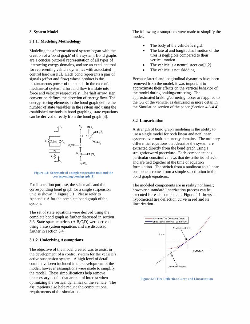
Modeling the aforementioned system began with the creation of a 'bond graph' of the system. Bond graphs

are a concise pictorial representation of all types of

interacting energy domains, and are an excellent tool

for representing vehicle dynamics with associated

control hardware[1]. Each bond represents a pair of

signals (effort and flow) whose product is the

instantaneous power of the bond. In the case of a

mechanical system, effort and flow translate into

force and velocity respectively. The 'half arrow' sign

convention defines the direction of energy flow. The

energy storing elements in the bond graph define the number of state variables in the system and using the

established methods in bond graphing, state equations

can be derived directly from the bond graph [4].

Figure 1.1: Schematic of a single suspension unit and the

corresponding bond graph [1]

For illustration purpose, the schematic and the

corresponding bond graph for a single suspension

unit is shown in Figure 3.1. Please refer to

Appendix A for the complete bond graph of the

system.

The set of state equations were derived using the

complete bond graph as further discussed in section

3.3. State-space matrices (A,B,C,D) were derived

using these system equations and are discussed

further in section 3.4.

3.1.2. Underlying Assumptions

The objective of the model created was to assist in

the development of a control system for the vehicle‘s

active suspension system. A high level of detail

could have been included in the development of the

model, however assumptions were made to simplify

the model. These simplifications help remove

unnecessary details that are not of interest when

optimizing the vertical dynamics of the vehicle. The assumptions also help reduce the computational

requirements of the simulation.

The following assumptions were made to simplify the

model:

The body of the vehicle is rigid.

The lateral and longitudinal motion of the

tires is negligible compared to their

vertical motion.

The vehicle is a neutral steer car[1,2]

The vehicle is not skidding

Because lateral and longitudinal dynamics have been

removed from the model, it was important to approximate their effects on the vertical behavior of

the model during braking/cornering. The

approximated braking/cornering forces are applied to

the CG of the vehicle, as discussed in more detail in

the Simulation section of the paper (Section 4.3-4.4).

3.2 Linearization

A strength of bond graph modeling is the ability to

use a single model for both linear and nonlinear

systems over multiple energy domains. The ordinary

differential equations that describe the system are

extracted directly from the bond graph using a

straightforward procedure. Each component has

particular constitutive laws that describe its behavior

and are tied together at the time of equation formulation. The switch from a nonlinear to a linear

component comes from a simple substitution in the

bond graph equations.

The modeled components are in reality nonlinear;

however a standard linearization process can be

executed for each component. Figure 4.1 shows a

hypothetical tire deflection curve in red and its linearization.

Figure 4.1: Tire Deflection Curve and Linearization

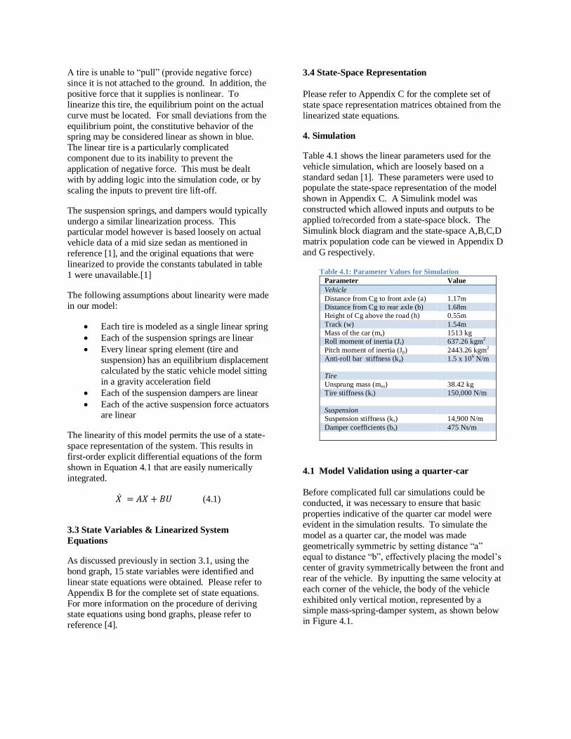
A tire is unable to ―pull‖ (provide negative force)

since it is not attached to the ground. In addition, the

positive force that it supplies is nonlinear. To

linearize this tire, the equilibrium point on the actual

curve must be located. For small deviations from the

equilibrium point, the constitutive behavior of the spring may be considered linear as shown in blue.

The linear tire is a particularly complicated

component due to its inability to prevent the

application of negative force. This must be dealt

with by adding logic into the simulation code, or by

scaling the inputs to prevent tire lift-off.

The suspension springs, and dampers would typically

undergo a similar linearization process. This particular model however is based loosely on actual

vehicle data of a mid size sedan as mentioned in

reference [1], and the original equations that were

linearized to provide the constants tabulated in table

1 were unavailable.[1]

The following assumptions about linearity were made

in our model:

Each tire is modeled as a single linear spring

Each of the suspension springs are linear

Every linear spring element (tire and

suspension) has an equilibrium displacement

calculated by the static vehicle model sitting

in a gravity acceleration field

Each of the suspension dampers are linear

Each of the active suspension force actuators are linear

The linearity of this model permits the use of a state-

space representation of the system. This results in

first-order explicit differential equations of the form

shown in Equation 4.1 that are easily numerically

integrated.

𝑋 = 𝐴𝑋 + 𝐵𝑈 (4.1)

3.3 State Variables & Linearized System

Equations

As discussed previously in section 3.1, using the

bond graph, 15 state variables were identified and

linear state equations were obtained. Please refer to

Appendix B for the complete set of state equations.

For more information on the procedure of deriving state equations using bond graphs, please refer to

reference [4].

3.4 State-Space Representation

Please refer to Appendix C for the complete set of

state space representation matrices obtained from the

linearized state equations.

4. Simulation

Table 4.1 shows the linear parameters used for the

vehicle simulation, which are loosely based on a

standard sedan [1]. These parameters were used to populate the state-space representation of the model

shown in Appendix C. A Simulink model was

constructed which allowed inputs and outputs to be

applied to/recorded from a state-space block. The

Simulink block diagram and the state-space A,B,C,D

matrix population code can be viewed in Appendix D

and G respectively.

Table 4.1: Parameter Values for Simulation

Parameter Value

Vehicle

Distance from Cg to front axle (a) 1.17m

Distance from Cg to rear axle (b) 1.68m

Height of Cg above the road (h) 0.55m

Track (w) 1.54m

Mass of the car (ms) 1513 kg

Roll moment of inertia (Jr) 637.26 kgm2

Pitch moment of inertia (Jp) 2443.26 kgm2

Anti-roll bar stiffness (ka) 1.5 x 106 N/m

Tire

Unsprung mass (mus) 38.42 kg

Tire stiffness (kt) 150,000 N/m

Suspension

Suspension stiffness (ks) 14,900 N/m

Damper coefficients (bs) 475 Ns/m

4.1 Model Validation using a quarter-car

Before complicated full car simulations could be

conducted, it was necessary to ensure that basic

properties indicative of the quarter car model were

evident in the simulation results. To simulate the

model as a quarter car, the model was made

geometrically symmetric by setting distance ―a‖

equal to distance ―b‖, effectively placing the model‘s

center of gravity symmetrically between the front and

rear of the vehicle. By inputting the same velocity at

each corner of the vehicle, the body of the vehicle

exhibited only vertical motion, represented by a simple mass-spring-damper system, as shown below

in Figure 4.1.

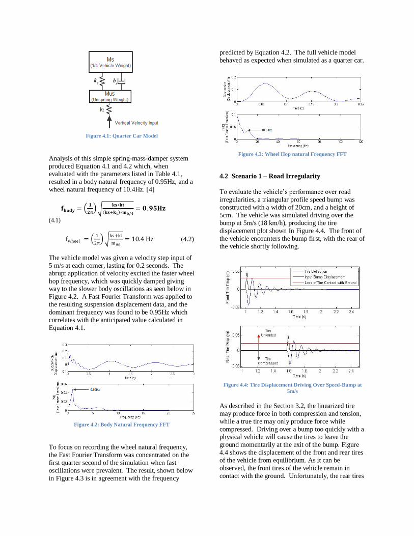
Figure 4.1: Quarter Car Model

Analysis of this simple spring-mass-damper system

produced Equation 4.1 and 4.2 which, when evaluated with the parameters listed in Table 4.1,

resulted in a body natural frequency of 0.95Hz, and a

wheel natural frequency of 10.4Hz. [4]

𝐟𝐛𝐨𝐝𝐲 = 𝟏

𝟐𝛑

𝐤𝐬∗𝐤𝐭

𝐤𝐬+𝐤𝐭 ∗𝐦𝐛/𝟒= 𝟎. 𝟗𝟓𝐇𝐳

(4.1)

fwheel = 1

2π

ks +kt

mus= 10.4 Hz (4.2)

The vehicle model was given a velocity step input of

5 m/s at each corner, lasting for 0.2 seconds. The

abrupt application of velocity excited the faster wheel

hop frequency, which was quickly damped giving way to the slower body oscillations as seen below in

Figure 4.2. A Fast Fourier Transform was applied to

the resulting suspension displacement data, and the

dominant frequency was found to be 0.95Hz which

correlates with the anticipated value calculated in

Equation 4.1.

Figure 4.2: Body Natural Frequency FFT

To focus on recording the wheel natural frequency,

the Fast Fourier Transform was concentrated on the

first quarter second of the simulation when fast

oscillations were prevalent. The result, shown below

in Figure 4.3 is in agreement with the frequency

predicted by Equation 4.2. The full vehicle model

behaved as expected when simulated as a quarter car.

Figure 4.3: Wheel Hop natural Frequency FFT

4.2 Scenario 1 – Road Irregularity

To evaluate the vehicle‘s performance over road

irregularities, a triangular profile speed bump was

constructed with a width of 20cm, and a height of

5cm. The vehicle was simulated driving over the

bump at 5m/s (18 km/h), producing the tire

displacement plot shown In Figure 4.4. The front of

the vehicle encounters the bump first, with the rear of

the vehicle shortly following.

Figure 4.4: Tire Displacement Driving Over Speed-Bump at

5m/s

As described in the Section 3.2, the linearized tire

may produce force in both compression and tension,

while a true tire may only produce force while

compressed. Driving over a bump too quickly with a physical vehicle will cause the tires to leave the

ground momentarily at the exit of the bump. Figure

4.4 shows the displacement of the front and rear tires

of the vehicle from equilibrium. As it can be

observed, the front tires of the vehicle remain in

contact with the ground. Unfortunately, the rear tires

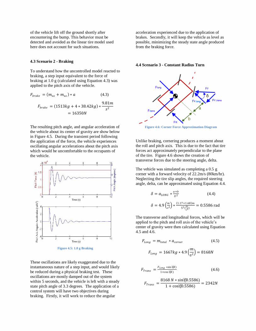
of the vehicle lift off the ground shortly after

encountering the bump. This behavior must be

detected and avoided as the linear tire model used

here does not account for such situations.

4.3 Scenario 2 - Braking

To understand how the uncontrolled model reacted to

braking, a step input equivalent to the force of

braking at 1.0 g (calculated using Equation 4.3) was

applied to the pitch axis of the vehicle.

𝐹𝑏𝑟𝑎𝑘𝑒 = 𝑚𝑢𝑠 + 𝑚𝑢𝑠 ∗ 𝑎 (4.3)

𝐹𝑏𝑟𝑎𝑘𝑒 = 1513𝑘𝑔 + 4 ∗ 38.42𝑘𝑔 ∗9.81𝑚

𝑠2

= 16350𝑁

The resulting pitch angle, and angular acceleration of

the vehicle about its center of gravity are show below

in Figure 4.5. During the transient period following

the application of the force, the vehicle experiences

oscillating angular accelerations about the pitch axis

which would be uncomfortable to the occupants of

the vehicle.

Figure 4.5: 1.0 g Braking

These oscillations are likely exaggerated due to the

instantaneous nature of a step input, and would likely

be reduced during a physical braking test. These

oscillations are mostly damped out of the system

within 5 seconds, and the vehicle is left with a steady

state pitch angle of 3.3 degrees. The application of a

control system will have two objectives during

braking. Firstly, it will work to reduce the angular

acceleration experienced due to the application of

brakes. Secondly, it will keep the vehicle as level as

possible, minimizing the steady state angle produced

from the braking force.

4.4 Scenario 3 - Constant Radius Turn

Figure 4.6: Corner Force Approximation Diagram

Unlike braking, cornering produces a moment about

the roll and pitch axis. This is due to the fact that tire

forces act approximately perpendicular to the plane

of the tire. Figure 4.6 shows the creation of

transverse forces due to the steering angle, delta.

The vehicle was simulated as completing a 0.5 g

corner with a forward velocity of 22.2m/s (80km/hr).

Neglecting the tire slip angles, the required steering

angle, delta, can be approximated using Equation 4.4.

𝛿 = 𝑎𝐿𝑂𝑁𝐺 ∗𝑎+𝑏

𝑈2 (4.4)

𝛿 = 4.9 𝑚

𝑠2 ∗

1.17+1.68 𝑚

52(𝑚

𝑠2)= 0.5586 rad

The transverse and longitudinal forces, which will be

applied to the pitch and roll axis of the vehicle‘s

center of gravity were then calculated using Equation

4.5 and 4.6.

𝐹𝐿𝑜𝑛𝑔 = 𝑚𝑡𝑜𝑡𝑎𝑙 ∗ 𝑎𝑐𝑜𝑟𝑛𝑒𝑟 (4.5)

𝐹𝐿𝑜𝑛𝑔 = 1667𝑘𝑔 ∗ 4.9 𝑚

𝑠2 = 8168𝑁

𝐹𝑇𝑟𝑎𝑛𝑠 =𝐹𝐿𝑜𝑛𝑔 ∗sin (𝛿)

1+cos (𝛿) (4.6)

𝐹𝑇𝑟𝑎𝑛𝑠 =8168 𝑁 ∗ sin(0.5586)

1 + cos(0.5586)= 2342𝑁

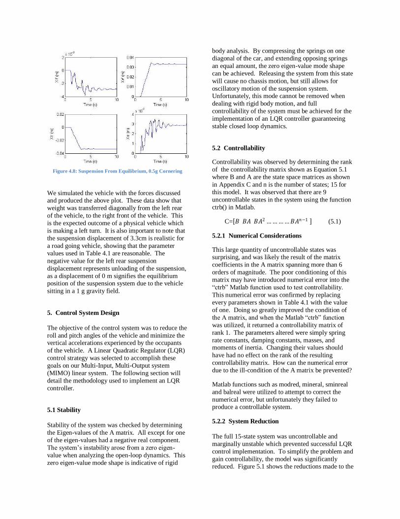
Figure 4.8: Suspension From Equilibrium, 0.5g Cornering

We simulated the vehicle with the forces discussed and produced the above plot. These data show that

weight was transferred diagonally from the left rear

of the vehicle, to the right front of the vehicle. This

is the expected outcome of a physical vehicle which

is making a left turn. It is also important to note that

the suspension displacement of 3.3cm is realistic for

a road going vehicle, showing that the parameter

values used in Table 4.1 are reasonable. The

negative value for the left rear suspension

displacement represents unloading of the suspension,

as a displacement of 0 m signifies the equilibrium position of the suspension system due to the vehicle

sitting in a 1 g gravity field.

5. Control System Design

The objective of the control system was to reduce the

roll and pitch angles of the vehicle and minimize the vertical accelerations experienced by the occupants

of the vehicle. A Linear Quadratic Regulator (LQR)

control strategy was selected to accomplish these

goals on our Multi-Input, Multi-Output system

(MIMO) linear system. The following section will

detail the methodology used to implement an LQR

controller.

5.1 Stability

Stability of the system was checked by determining

the Eigen-values of the A matrix. All except for one

of the eigen-values had a negative real component.

The system‘s instability arose from a zero eigen-

value when analyzing the open-loop dynamics. This

zero eigen-value mode shape is indicative of rigid

body analysis. By compressing the springs on one

diagonal of the car, and extending opposing springs

an equal amount, the zero eigen-value mode shape

can be achieved. Releasing the system from this state

will cause no chassis motion, but still allows for

oscillatory motion of the suspension system. Unfortunately, this mode cannot be removed when

dealing with rigid body motion, and full

controllability of the system must be achieved for the

implementation of an LQR controller guaranteeing

stable closed loop dynamics.

5.2 Controllability

Controllability was observed by determining the rank

of the controllability matrix shown as Equation 5.1

where B and A are the state space matrices as shown

in Appendix C and n is the number of states; 15 for

this model. It was observed that there are 9

uncontrollable states in the system using the function

ctrb() in Matlab.

C= 𝐵 𝐵𝐴 𝐵𝐴2 …………𝐵𝐴𝑛−1 (5.1)

5.2.1 Numerical Considerations

This large quantity of uncontrollable states was surprising, and was likely the result of the matrix

coefficients in the A matrix spanning more than 6

orders of magnitude. The poor conditioning of this

matrix may have introduced numerical error into the

―ctrb‖ Matlab function used to test controllability.

This numerical error was confirmed by replacing

every parameters shown in Table 4.1 with the value

of one. Doing so greatly improved the condition of

the A matrix, and when the Matlab ―ctrb‖ function

was utilized, it returned a controllability matrix of

rank 1. The parameters altered were simply spring

rate constants, damping constants, masses, and moments of inertia. Changing their values should

have had no effect on the rank of the resulting

controllability matrix. How can the numerical error

due to the ill-condition of the A matrix be prevented?

Matlab functions such as modred, mineral, sminreal

and balreal were utilized to attempt to correct the

numerical error, but unfortunately they failed to produce a controllable system.

5.2.2 System Reduction

The full 15-state system was uncontrollable and

marginally unstable which prevented successful LQR

control implementation. To simplify the problem and

gain controllability, the model was significantly reduced. Figure 5.1 shows the reductions made to the

system bond graph. These reductions are analogues

to removing the tires and un-sprung mass of the

vehicle. The vehicle‘s suspension was now modeled

as being attached directly to the road surface. The

simplified model reduced the number of states from

15 to only 7.

Figure 5.1: Simplified Bond Graph

Before the simplified model could be controlled, it

was necessary to investigate how it performed

compared to the original model. Figure 5.2 shows the original and simplified models‘ suspension

response to the bump input discussed previously in

Section 4.2. The abrupt application of the bump

excited high speed oscillations in the original model

due to the wheel hop natural frequency of the un-

sprung mass discussed in Section 4.1. The simplified

model removes the un-sprung mass as well as the tire

spring, and does not exhibit high speed oscillations.

The high speed oscillations are quickly damped out,

leaving only the slow speed body oscillations. Both

the original and simplified model exhibit similar slow

speed body oscillatory motion, but the removal of the high speed dynamics from the system makes the

simplified model unsuitable for controllers designed

for bump disturbances.

Figure 5.2: Original and Simplified Model Response to “Speed

Bump”

The simplified model is however suitable for

controllers designed against cornering and braking

disturbances. Figure 5.3 shows the two models‘

response to a step input equivalent to 1g of braking

force. The simplified model closely approximated

the original model‘s dynamics. Removing the tire springs effectively removed a spring in series, which

stiffened the simplified model slightly. It is no

surprise that the simplified model exhibited slightly

less steady state pitch when compared to the original

model. The simplified model is suitable for

controllers designed to encounter cornering and

braking disturbances.

Figure 5.3: Original and Simplified Model Response to a 1g

Braking Disturbance

5.2.3 Controllable Input “Trick”

Unfortunately, the reduced system had a

controllability matrix with rank 6 out of 7 total states.

The four force actuators situated at each corner of the

vehicle were not capable of fully controlling the

system. To attempt to gain controllability, the

exogenous inputs were included with the controllable

inputs in the formulation of the controllability matrix. The inclusion of these extra inputs produced a full

rank controllability matrix, and LQR control could be

designed.

It is important to note that the inclusion of inputs,

which the system will have no control over, into the

formulation of an LQR controller has broken the

theory guaranteeing stable closed loop dynamics.

The next section will detail precautions taken to minimize the risk of instability.

5.3 LQR Controller Design

The optimal state-feedback controller, Linear

Quadratic Regulator was considered the best solution

for the following reasons.

1. The system is modeled as Linear and it

is Time Invariant (LTI).

2. The desired state does not vary with

time and it is constant at equilibrium.

(Regulator problem. Not a tracking

problem.)

3. The need to minimize the actuator

force and thus actuator power consumption.

The use of a LQR controller allowed us to achieve all

our performance requirements as discussed in Section

5.3.1.

5.3.1 Design Goals

As discussed previously, the main goal of an active suspension system is to keep the vehicle as level as

possible while minimizing the vertical accelerations

caused due to road inputs. The passenger

acceleration has been used here as an indicator of ride

comfort. Therefore the effort was taken to keep the

vertical acceleration within 0.98 ms-2.

To quantify these abstract design goals commercial systems such as the Bose Suspension System [6] and

systems discussed in reference [8] and [9] were

compared. Suspension spring deflection limits were

dictated by the actual mechanical limits of a

suspension system in a mid-size sedan. The

parameters chosen represent the maximums that a

driver is expected to encounter in non-emergency

situations, and a driver is unlikely to physically

perceive angles less than one degree. The finalized

design goals are shown in Table 5.1.

Table 5.1 : Controller Design Goals

Parameter Value

Vehicle Pitch 1.0 deg. max.

Vehicle Roll 1.0 deg. max.

Sprung mass acceleration 0.98 ms-2 max.

Suspension Spring deflection 0.2 m

Settling Time within 0.25s

Rise Time Within 0.1s

5.3.2 State-Space Expansion

The control system design objectives discussed in

Section 5.3.1 focus on the pitch and roll angles of the

model. Unfortunately, the 7-state representation of

the model had pitch and roll angular velocity states.

To allow the controller to directly target the body

angles, instead of angular velocities, the state-space

representation of the model was expanded by two

states, pitch angle and roll angle. Equations 5.1 and

5.2 show the two additional state equations.

𝜔𝑝 = 𝜃𝑝 = 𝐿𝑝/𝐽𝑝 (5.1)

𝜔𝑟 = 𝜃𝑟 = 𝐿𝑟/𝐼𝑟 (5.2)

5.3.3 Quadratic Cost Function

The cost function used to generate the LQR gain

matrix is shown below in Equation 5.3.

𝐽 = 𝑥𝑇𝑅𝑥 + 𝑢𝑇𝛬𝑢 𝑑𝑡𝑇

𝑜 (5.3)

The state and input penalization matrices are shown

as Equations 5.4 and 5.5.

𝑅 =

11

11

11

1𝑃

𝑅

(5.4)

𝛬 =

1𝑒5

1𝑒51𝑒5

1𝑒51𝑒5

1𝑒51

11

1

(5.5)

All off diagonal terms in the state and input

penalization matrices were left as zero. These terms

represent penalization of combinations of different

states or inputs. The first six diagonal terms of the

input weighting matrix (R) penalize the use of the

exogenous inputs, of which the controller has no

physical control over. To minimize the use of such

inputs, they were penalized by five orders of

magnitude compared to the four force actuator inputs

which can actually be controlled. The effects of this

penalization are discussed in Section 6.1.2.

The 8th and 9th diagonal coefficients of the state

weighting matrix represent the penalization of pitch

angle and roll angle respectively. By changing the

weighting of these coefficients compared to the other

coefficients in the input and state weighting matrices,

the closed loop dynamics of the system may be

augmented.

Using the input and state weighting matrices, in

conjunction with the open loop A and B matrices of

the reduced system, a gain matrix, K, was generated

using Matlab‘s LQR command.

5.3.4 LQR Controller Implementation

The Simulink model used to implement the gain

matrix produced by the matlab LQR routine can be

found in Appendix E. Disturbances are fed into the

state-space block, which transforms them into outputs

based on the open loop system dynamics. The

outputs are then fed back into the gain matrix produced by the LQR Matlab routine. This gain

matrix transforms the outputs of the system into

desired inputs to control the system, which are fed

back into the state-space block.

Two control architecture scenarios were studied. The

first allowed for control over the four force actuators,

as well as the six exogenous inputs. In reality, the

controller would have no influence over the six exogenous inputs, and the second scenario severs this

connection.

6. Controlled Results

This sections studies the effects of removing the link

between the controller and the six exogenous inputs which it does not physically have control over. The

pitch and roll weighting coefficients were set to the

relatively large values of 1,000,000 so that the

controller would work to minimize the pitch and roll

angles of the car.

6.1 Scenario 1: Ten Controllable Inputs

The LQR controller was designed with a B matrix

allowing for control over all ten inputs (including the

6 exogenous inputs). This section studies the effects

of allowing the feedback control of all 10 inputs.

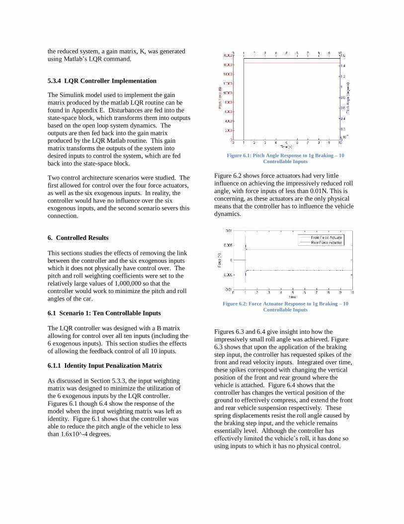
6.1.1 Identity Input Penalization Matrix

As discussed in Section 5.3.3, the input weighting matrix was designed to minimize the utilization of

the 6 exogenous inputs by the LQR controller.

Figures 6.1 though 6.4 show the response of the

model when the input weighting matrix was left as

identity. Figure 6.1 shows that the controller was

able to reduce the pitch angle of the vehicle to less

than 1.6x10^-4 degrees.

Figure 6.1: Pitch Angle Response to 1g Braking – 10

Controllable Inputs

Figure 6.2 shows force actuators had very little

influence on achieving the impressively reduced roll

angle, with force inputs of less than 0.01N. This is

concerning, as these actuators are the only physical

means that the controller has to influence the vehicle

dynamics.

Figure 6.2: Force Actuator Response to 1g Braking – 10

Controllable Inputs

Figures 6.3 and 6.4 give insight into how the

impressively small roll angle was achieved. Figure

6.3 shows that upon the application of the braking

step input, the controller has requested spikes of the

front and read velocity inputs. Integrated over time,

these spikes correspond with changing the vertical

position of the front and rear ground where the

vehicle is attached. Figure 6.4 shows that the controller has changes the vertical position of the

ground to effectively compress, and extend the front

and rear vehicle suspension respectively. These

spring displacements resist the roll angle caused by

the braking step input, and the vehicle remains

essentially level. Although the controller has

effectively limited the vehicle‘s roll, it has done so

using inputs to which it has no physical control.

Figure 6.3: Ground Velocity Input Response to 1g Braking –

10 Controllable Inputs

Figure 6.4: Suspension Displacement Response to 1g Braking –

10 Controllable Inputs

6.1.2 Weighted Input Penalization Matrix

This section utilizes the input weighting matrix

discussed in Section 5.3.3 which heavily penalizes

the use of the six exogenous inputs for controlling the

system. Figure 6.5 shows that with the updated

penalization matrix the controllers performance at

reducing the pitch angle of the vehicle has been

slightly reduced compared to the previous scenario.

Figure 6.5: Pitch Angle Response to 1g Braking – 10

Controllable Inputs

The maximum roll angle of 0.04 degrees is however

well within the design goals discussed in Section

5.3.1.

Figure 6.6 shows that the controller has began to

utilize the four force actuators to limit vehicle pitch

angle. Unfortunately, Figure 6.7 shows that the

controller has still relied heavily on manipulating the

ground velocity inputs in limiting vehicle pitch.

Figure 6.6: Force Actuator Input Response to 1g Braking – 10

Controllable Inputs

Figure 6.7: Suspension Displacement Response to 1g Braking –

10 Controllable Inputs

6.2 Scenario 2: 4 Controllable Inputs

This section discusses the ramifications of removing

the link between the controller, and the 6 exogenous

inputs. To accomplish this, the bond highlighted in

red in the Simulink model (shown in Appendix F) has

been removed. When this model is executed, Matlab

returns a warning, but successfully simulates the model.

6.2.1 Identity Input Penalization Matrix

With an identity input weighting matrix, the LQR

controller relies heavily on the 6 exogenous inputs

when designing the gain matrix used to control the

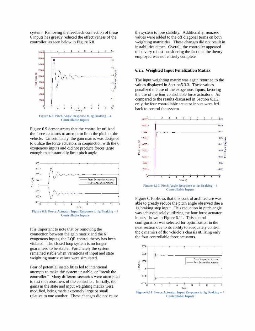
system. Removing the feedback connection of these

6 inputs has greatly reduced the effectiveness of the

controller, as seen below in Figure 6.8.

Figure 6.8: Pitch Angle Response to 1g Braking – 4

Controllable Inputs

Figure 6.9 demonstrates that the controller utilized

the force actuators to attempt to limit the pitch of the

vehicle. Unfortunately, the gain matrix was designed

to utilize the force actuators in conjunction with the 6

exogenous inputs and did not produce forces large enough to substantially limit pitch angle.

Figure 6.9: Force Actuator Input Response to 1g Braking – 4

Controllable Inputs

It is important to note that by removing the

connection between the gain matrix and the 6

exogenous inputs, the LQR control theory has been violated. The closed loop system is no longer

guaranteed to be stable. Fortunately the system

remained stable when variations of input and state

weighting matrix values were simulated.

Fear of potential instabilities led to intentional

attempts to make the system unstable, or ―break the

controller.‖ Many different scenarios were attempted

to test the robustness of the controller. Initially, the gains in the state and input weighting matrix were

modified, being made extremely large or small

relative to one another. These changes did not cause

the system to lose stability. Additionally, nonzero

values were added to the off diagonal terms on both

weighting matricides. These changes did not result in

instabilities either. Overall, the controller appeared

to be very robust considering the fact that the theory

employed was not entirely complete.

6.2.2 Weighted Input Penalization Matrix

The input weighting matrix was again returned to the

values displayed in Section5.3.3. These values

penalized the use of the exogenous inputs, favoring

the use of the four controllable force actuators. As compared to the results discussed in Section 6.1.2,

only the four controllable actuator inputs were fed

back to control the system.

Figure 6.10: Pitch Angle Response to 1g Braking – 4

Controllable Inputs

Figure 6.10 shows that this control architecture was

able to greatly reduce the pitch angle observed due a

1g braking step input. This reduction in pitch angle

was achieved solely utilizing the four force actuator

inputs, shown in Figure 6.11. This control

configuration was selected for optimization in the

next section due to its ability to adequately control

the dynamics of the vehicle‘s chassis utilizing only

the four controllable force actuators.

Figure 6.11: Force Actuator Input Response to 1g Braking – 4

Controllable Inputs

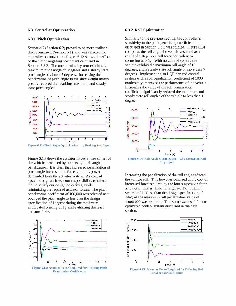
6.3 Controller Optimization

6.3.1 Pitch Optimization

Scenario 2 (Section 6.2) proved to be more realistic then Scenario 1 (Section 6.1), and was selected for

controller optimization. Figure 6.12 shows the effect

of the pitch weighting coefficient discussed in

Section 5.3.3. The uncontrolled system exhibited a

maximum pitch angle of 8degrees and a steady state

pitch angle of almost 5 degrees. Increasing the

penalization of pitch angle in the state weight matrix

greatly reduced the resulting maximum and steady

state pitch angles.

Figure 6.12: Pitch Angle Optimization – 1g Braking Step Input

Figure 6.13 shows the actuator forces at one corner of

the vehicle, produced by increasing pitch angle

penalization. It is clear that increased penalization of pitch angle increased the force, and thus power

demanded from the actuator system. As control

system designers it was our responsibility to select

―P‖ to satisfy our design objectives, while

minimizing the required actuator forces. The pitch

penalization coefficient of 100,000 was selected as it

bounded the pitch angle to less than the design

specification of 1degree during the maximum

anticipated braking of 1g while utilizing the least

actuator force.

Figure 6.13: Actuator Force Required for Differing Pitch

Penalization Coefficients

6.3.2 Roll Optimization

Similarly to the previous section, the controller‘s sensitivity to the pitch penalizing coefficient

discussed in Section 5.3.3 was studied. Figure 6.14

compares the roll angle the vehicle assumed as a

result of a step input roll force equivalent to

cornering at 0.5g. With no control system, the

vehicle exhibited a maximum roll angle of 12

degrees, and a steady state roll angle of more than 7

degrees. Implementing an LQR derived control

system with a roll penalization coefficient of 1000

moderately improved the performance of the vehicle.

Increasing the value of the roll penalization

coefficient significantly reduced the maximum and steady state roll angles of the vehicle to less than 1

degree.

Figure 6.14: Roll Angle Optimization – 0.5g Cornering Roll

Step Input

Increasing the penalization of the roll angle reduced

the vehicle roll. This however occurred at the cost of

increased force required by the four suspension force

actuators. This is shown in Figure 6.15. To limit

vehicle roll to less than the design specification of

1degree the maximum roll penalization value of

1,000,000 was required. This value was used for the

optimized control system discussed in the next section.

Figure 6.15: Actuator Force Required for Differing Roll

Penalization Coefficients

7. Optimum Controller

The optimum controller was selected with input and

state weighting matrices shown in Section 5.3.3. The

vehicle was simulated cornering at 0.5g, which

produced a rolling force of 8168N and a pitching force of 2342N as discussed in Section 4.4. Figures

7.1 and 7.2 show that the controller has limited

vehicle pitch and roll to well within the design

specifications discussed in Section 5.3.1.

Figure 7.1: Optimum Vehicle Pitch Force and Angle Response

Figure 7.2: Optimum Vehicle Roll Force and Angle Response

The required actuator forces from each corner of the

vehicle are shown below in Figure 7.3. As expected,

the right front and left rear actuators are required to

supply a larger amount of force due to the diagonal

weight transfer phenomenon discussed in Section 4.4.

Figure 7.3: Optimum Actuator Force Responses

Unfortunately, the limitation of the non-linear tire

model discussed in Section 3.2 may have been

exceeded. Figure 7.3 displays the left rear force

actuator exerting a tension force of 2000N. This

tension force can be no larger than the corner weight

of the vehicle, or else the physical tire may lift off of the ground. Based on the parameters discussed in

4.1, 41% of the 1513kg vehicle mass is statically

situated over the rear axle. This is equivalent to a

static mass of 310.6kg equating to 3047N of force

applied statically to the left rear corner of the vehicle

due to gravity. This means that the left rear force

actuator may request no more than 3047N of tensile

force from the static vehicle, or else the tire will lift

off the ground.

Unfortunately, the dynamic vehicle assumes a

different weight distribution then the static vehicle.

Further investigation is necessary to ensure that the

linear tire model is not operated in its unrealistic

region detailed in Figure 4.1. This analysis is

complicated by the removal of the tire model, and tire

deflection states when the model was simplified.

If it was determined that the tires were at risk of

being operating outside of their linearly acceptable

region, a more complicated control system may be

required. This system would need to sense the

approach of tire lifting, and change its control

algorithms to avoid such a phenomenon. Such a

control system was deemed outside the scope of this

project.

8. Conclusions

A linear vehicle dynamics model has been

constructed which focuses on the vertical motion of a

vehicle due to road irregularities. This model avoids

the use of complicated lateral/longitudinal vehicle dynamics, and instead approximated their application

to the CG of the vehicle.

The model has been validated in quarter car, and full

car simulations. The model successfully

approximated bump, brake, and cornering situations.

Future work will be to improve passenger ride

comfort by implementing an active suspension

control system. This improvement will be

accomplished through the utilization of force

actuators tied into each corner of the vehicle‘s

suspension system.

6. References

[1] Bose Corporation. The Bose Suspension

System (2004).

http://www.bose.com/pdf/technologies/bose

_suspension_system.pdf) [2] Shim, Taehyun, Magolis, Donald (2001).

―A bond graph model incorporating sensors,

actuators, and vehicle dynamics for

developing controllers for vehicle safety,‖

Journal of the Franklin Institute 338 (2001)

pp.21-34

[3] Milliken, Douglas L., Milliken, William F.

Race Car Vehicle Dynamics, SAE

International (2003).

[4] Karnopp, Dean(1976). ―Bond Graphs for

Vehicle Dynamics,‖ Vehicle System Dynamics, 5: 3, 171 — 184

[5] Karnopp, Dean C., Margolis, Donald L.

Rosenberg, Ronald C. System Dynamics –

Modeling and Simulation of Mechatronic

Systems. 4th ed. New York : John Wiley

(2006)

[6] Karnopp, Dean C., Margolis, Donald L.

Engineering Applications of Dynamics. New

York : John Wiley (2007)

[7] Sam, Y.M., Ghani, M.R.H.A, Ahmad, N.

(2000). ―LQR controller for active car

suspension‖ TENCON 2000 Proceedings

Volume 1. pp.441-444 [8] Hrovat, D., ―Applications of Optimal

Control to Advanced Automotive

Suspension Design,‖ J. of Dynamic

Systems, Measurement, and Control, Vol.

115, No.2(B), June 1993, pp.328-342.

[9] Zhang, B. Fan M, Miao F., ―Optimal

Control of Vehicle Active Suspension

Systems with Actuator Delay,‖ 2007 IEEE

International Conference on Control and

Automation, Guangzhou, CHINA - June

2007.

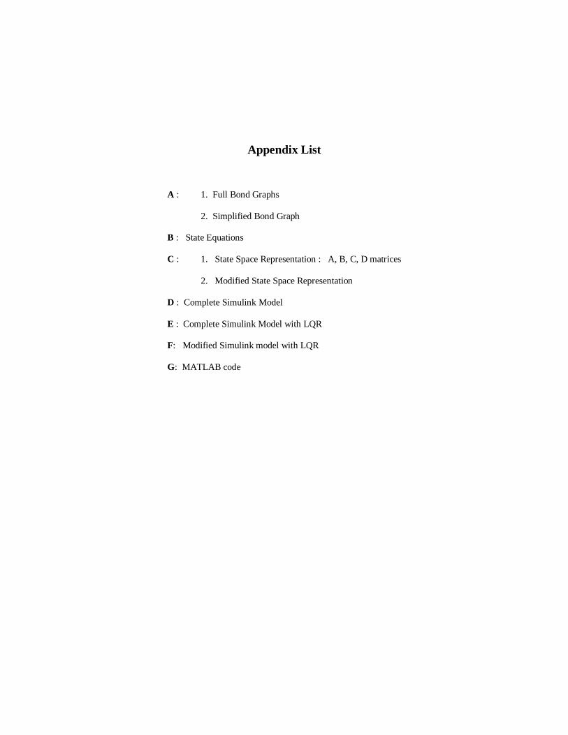
Appendix List

A : 1. Full Bond Graphs

2. Simplified Bond Graph

B : State Equations

C : 1. State Space Representation : A, B, C, D matrices

2. Modified State Space Representation

D : Complete Simulink Model

E : Complete Simulink Model with LQR

F: Modified Simulink model with LQR

G: MATLAB code

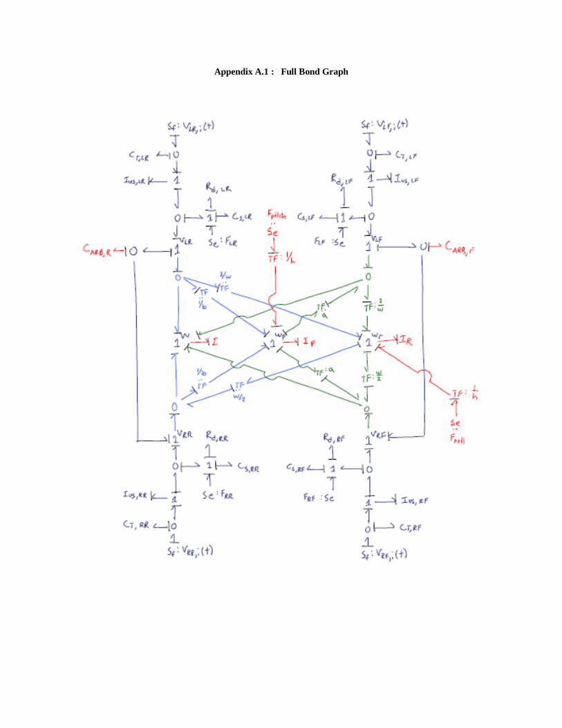
Appendix A.1 : Full Bond Graph

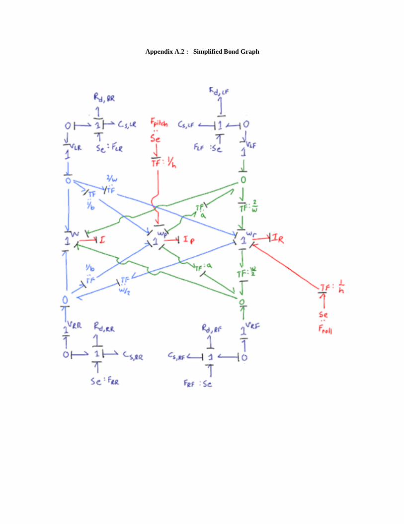
Appendix A.2 : Simplified Bond Graph

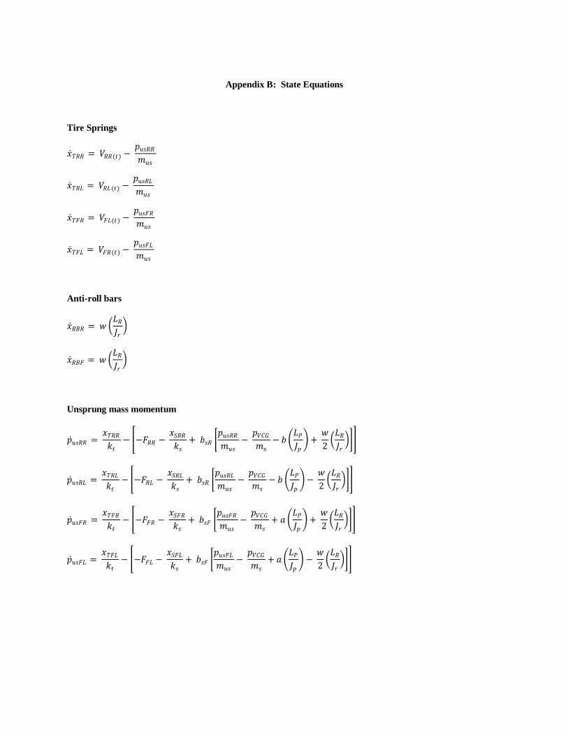
Appendix B: State Equations

Tire Springs

𝑥 𝑇𝑅𝑅 = 𝑉𝑅𝑅(𝑡) − 𝑝𝑢𝑠𝑅𝑅

𝑚𝑢𝑠

𝑥 𝑇𝑅𝐿 = 𝑉𝑅𝐿(𝑡) − 𝑝𝑢𝑠𝑅𝐿

𝑚𝑢𝑠

𝑥 𝑇𝐹𝑅 = 𝑉𝐹𝐿(𝑡) − 𝑝𝑢𝑠𝐹𝑅

𝑚𝑢𝑠

𝑥 𝑇𝐹𝐿 = 𝑉𝐹𝑅(𝑡) − 𝑝𝑢𝑠𝐹𝐿

𝑚𝑢𝑠

Anti-roll bars

𝑥 𝑅𝐵𝑅 = 𝑤 𝐿𝑅

𝐽𝑟

𝑥 𝑅𝐵𝐹 = 𝑤 𝐿𝑅

𝐽𝑟

Unsprung mass momentum

𝑝 𝑢𝑠𝑅𝑅 = 𝑥𝑇𝑅𝑅

𝑘𝑡

− −𝐹𝑅𝑅 − 𝑥𝑆𝑅𝑅

𝑘𝑠

+ 𝑏𝑠𝑅 𝑝𝑢𝑠𝑅𝑅

𝑚𝑢𝑠

− 𝑝𝑉𝐶𝐺

𝑚𝑠

− 𝑏 𝐿𝑃

𝐽𝑝 +

𝑤

2 𝐿𝑅

𝐽𝑟

𝑝 𝑢𝑠𝑅𝐿 = 𝑥𝑇𝑅𝐿

𝑘𝑡

− −𝐹𝑅𝐿 − 𝑥𝑆𝑅𝐿

𝑘𝑠

+ 𝑏𝑠𝑅 𝑝𝑢𝑠𝑅𝐿

𝑚𝑢𝑠

− 𝑝𝑉𝐶𝐺

𝑚𝑠

− 𝑏 𝐿𝑃

𝐽𝑝 −

𝑤

2 𝐿𝑅

𝐽𝑟

𝑝 𝑢𝑠𝐹𝑅 = 𝑥𝑇𝐹𝑅

𝑘𝑡

− −𝐹𝐹𝑅 − 𝑥𝑆𝐹𝑅

𝑘𝑠

+ 𝑏𝑠𝐹 𝑝𝑢𝑠𝐹𝑅

𝑚𝑢𝑠

− 𝑝𝑉𝐶𝐺

𝑚𝑠

+ 𝑎 𝐿𝑃

𝐽𝑝 +

𝑤

2 𝐿𝑅

𝐽𝑟

𝑝 𝑢𝑠𝐹𝐿 = 𝑥𝑇𝐹𝐿

𝑘𝑡

− −𝐹𝐹𝐿 − 𝑥𝑆𝐹𝐿

𝑘𝑠

+ 𝑏𝑠𝐹 𝑝𝑢𝑠𝐹𝐿

𝑚𝑢𝑠

− 𝑝𝑉𝐶𝐺

𝑚𝑠

+ 𝑎 𝐿𝑃

𝐽𝑝 −

𝑤

2 𝐿𝑅

𝐽𝑟

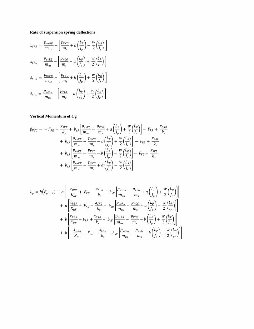
Rate of suspension spring deflections

𝑥 𝑆𝑅𝑅 = 𝑝𝑢𝑠𝑅𝑅

𝑚𝑢𝑠

− 𝑝𝑉𝐶𝐺

𝑚𝑠

+ 𝑏 𝐿𝑃

𝐽𝑝 −

𝑤

2 𝐿𝑅

𝐽𝑟

𝑥 𝑆𝑅𝐿 = 𝑝𝑢𝑠𝑅𝐿

𝑚𝑢𝑠

− 𝑝𝑉𝐶𝐺

𝑚𝑠

− 𝑎 𝐿𝑃

𝐽𝑝 +

𝑤

2 𝐿𝑅

𝐽𝑟

𝑥 𝑆𝐹𝑅 = 𝑝𝑢𝑠𝐹𝑅

𝑚𝑢𝑠

− 𝑝𝑉𝐶𝐺

𝑚𝑠

+ 𝑏 𝐿𝑃

𝐽𝑝 +

𝑤

2 𝐿𝑅

𝐽𝑟

𝑥 𝑆𝐹𝐿 = 𝑝𝑢𝑠𝐹𝐿

𝑚𝑢𝑠

− 𝑝𝑉𝐶𝐺

𝑚𝑠

− 𝑎 𝐿𝑃

𝐽𝑝 +

𝑤

2 𝐿𝑅

𝐽𝑟

Vertical Momentum of Cg

𝑝 𝑉𝐶𝐺 = − 𝐹𝐹𝑅 − 𝑥𝑆𝐹𝑅

𝑘𝑠

+ 𝑏𝑠𝐹 𝑝𝑢𝑠𝐹𝐿

𝑚𝑢𝑠

− 𝑝𝑉𝐶𝐺

𝑚𝑠

+ 𝑎 𝐿𝑃

𝐽𝑝 +

𝑤

2 𝐿𝑅

𝐽𝑟 − 𝐹𝑅𝑅 +

𝑥𝑆𝑅𝑅

𝑘𝑠

+ 𝑏𝑠𝐹 𝑝𝑢𝑠𝑅𝑅

𝑚𝑢𝑠

− 𝑝𝑉𝐶𝐺

𝑚𝑠

− 𝑏 𝐿𝑃

𝐽𝑝 +

𝑤

2 𝐿𝑅

𝐽𝑟 − 𝐹𝑅𝐿 +

𝑥𝑆𝑅𝐿

𝑘𝑠

+ 𝑏𝑠𝑅 𝑝𝑢𝑠𝑅𝐿

𝑚𝑢𝑠

− 𝑝𝑉𝐶𝐺

𝑚𝑠

− 𝑏 𝐿𝑃

𝐽𝑝 −

𝑤

2 𝐿𝑅

𝐽𝑟 − 𝐹𝐹𝐿 +

𝑥𝑆𝐹𝐿

𝑘𝑠

+ 𝑏𝑠𝑅 𝑝𝑢𝑠𝐹𝑅

𝑚𝑢𝑠

− 𝑝𝑉𝐶𝐺

𝑚𝑠

+ 𝑎 𝐿𝑃

𝐽𝑝 −

𝑤

2 𝐿𝑅

𝐽𝑟

𝐿 𝑝 = ℎ 𝐹𝑝𝑖𝑡𝑐 ℎ + 𝑎 −𝑥𝑅𝐵𝐹

𝐾𝑅𝐹

+ 𝐹𝐹𝑅 − 𝑥𝑆𝐹𝑅

𝑘𝑠

− 𝑏𝑠𝐹 𝑝𝑢𝑠𝐹𝑅

𝑚𝑢𝑠

− 𝑝𝑉𝐶𝐺

𝑚𝑠

+ 𝑎 𝐿𝑃

𝐽𝑝 +

𝑤

2 𝐿𝑅

𝐽𝑟

+ 𝑎 𝑥𝑅𝐵𝐹

𝐾𝑅𝐹

+ 𝐹𝐹𝐿 − 𝑥𝑆𝐹𝐿

𝑘𝑠

− 𝑏𝑠𝑅 𝑝𝑢𝑠𝐹𝐿

𝑚𝑢𝑠

− 𝑝𝑉𝐶𝐺

𝑚𝑠

+ 𝑎 𝐿𝑃

𝐽𝑝 −

𝑤

2 𝐿𝑅

𝐽𝑟

+ 𝑏 𝑥𝑅𝐵𝑅

𝐾𝑅𝑅

− 𝐹𝑅𝑅 +𝑥𝑆𝑅𝑅

𝑘𝑠

+ 𝑏𝑠𝐹 𝑝𝑢𝑠𝑅𝑅

𝑚𝑢𝑠

− 𝑝𝑉𝐶𝐺

𝑚𝑠

− 𝑏 𝐿𝑃

𝐽𝑝 +

𝑤

2 𝐿𝑅

𝐽𝑟

+ 𝑏 −𝑥𝑅𝐵𝑅

𝐾𝑅𝑅

− 𝐹𝑅𝐿 − 𝑥𝑆𝑅𝐿

𝑘𝑠

+ 𝑏𝑠𝑅 𝑝𝑢𝑠𝑅𝐿

𝑚𝑢𝑠

− 𝑝𝑉𝐶𝐺

𝑚𝑠

− 𝑏 𝐿𝑃

𝐽𝑝 −

𝑤

2 𝐿𝑅

𝐽𝑟

𝐿 𝑅 = ℎ 𝐹𝑟𝑜𝑙𝑙 − 𝑤

2 𝑥𝑅𝐵𝑅

𝐾𝑅𝐹

− 𝐹𝐹𝑅 + 𝑥𝑆𝐹𝑅

𝑘𝑠

+ 𝑏𝑠𝐹 𝑝57

𝑚𝑢𝑠

− 𝑝𝑉𝐶𝐺

𝑚𝑠

+ 𝑎 𝐿𝑃

𝐽𝑝 +

𝑤

2 𝐿𝑅

𝐽𝑟

− 𝑤

2 𝑥𝑅𝐵𝑅

𝐾𝑅𝐹

+ 𝐹𝐹𝐿 − 𝑥𝑆𝐹𝐿

𝑘𝑠

− 𝑏𝑠𝐹 𝑝32

𝑚𝑢𝑠

− 𝑝𝑉𝐶𝐺

𝑚𝑠

+ 𝑎 𝐿𝑃

𝐽𝑝 −

𝑤

2 𝐿𝑅

𝐽𝑟

−𝑤

2 𝑥𝑅𝐵𝐹

𝐾𝑅𝑅

− 𝐹𝑅𝑅 +𝑥𝑆𝑅𝑅

𝑘𝑠

+ 𝑏𝑠𝑅 𝑝𝑢𝑠𝑅𝑅

𝑚𝑢𝑠

− 𝑝𝑉𝐶𝐺

𝑚𝑠

− 𝑏 𝐿𝑃

𝐽𝑝 +

𝑤

2 𝐿𝑅

𝐽𝑟

− 𝑤

2 −

𝑥𝑅𝐵𝐹

𝐾𝑅𝑅

− 𝐹𝑅𝐿 − 𝑥𝑆𝑅𝐿

𝑘𝑠

+ 𝑏𝑠𝑅 𝑝𝑢𝑠𝑅𝐿

𝑚𝑢𝑠

− 𝑝𝑉𝐶𝐺

𝑚𝑠

− 𝑏 𝐿𝑃

𝐽𝑝 −

𝑤

2 𝐿𝑅

𝐽𝑟

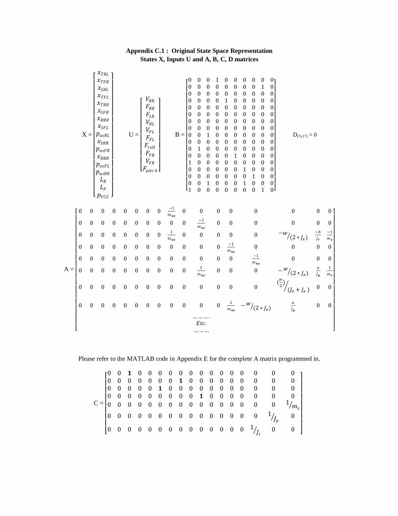
Appendix C.1 : Original State Space Representation

States X, Inputs U and A, B, C, D matrices

X =

𝑥𝑇𝑅𝐿

𝑥𝑇𝐹𝑅

𝑥𝑆𝑅𝐿

𝑥𝑇𝐹𝐿

𝑥𝑇𝑅𝑅

𝑥𝑆𝐹𝑅

𝑥𝑅𝐵𝑅

𝑥𝑆𝐹𝐿

𝑝𝑢𝑠𝑅𝐿

𝑥𝑆𝑅𝑅

𝑝𝑢𝑠𝐹𝑅

𝑥𝑅𝐵𝑅

𝑝𝑢𝑠𝐹𝐿

𝑝𝑢𝑠𝑅𝑅

𝐿𝑅

𝐿𝑃

𝑝𝑉𝐶𝐺

U =

𝑉𝑅𝑅

𝐹𝑅𝑅

𝐹𝐿𝑅

𝑉𝑅𝐿

𝑉𝐹𝐿

𝐹𝐹𝐿

𝐹𝑟𝑜𝑙𝑙

𝐹𝐹𝑅

𝑉𝐹𝑅

𝐹𝑝𝑖𝑡𝑐 ℎ

B =

0 0 0 1 0 0 0 0 0 00 0 0 0 0 0 0 0 1 00 0 0 0 0 0 0 0 0 00 0 0 0 1 0 0 0 0 00 0 0 0 0 0 0 0 0 00 0 0 0 0 0 0 0 0 00 0 0 0 0 0 0 0 0 00 0 0 0 0 0 0 0 0 00 0 1 0 0 0 0 0 0 00 0 0 0 0 0 0 0 0 00 1 0 0 0 0 0 0 0 00 0 0 0 0 1 0 0 0 01 0 0 0 0 0 0 0 0 00 0 0 0 0 0 1 0 0 00 0 0 0 0 0 0 1 0 00 0 1 0 0 0 1 0 0 01 0 0 0 0 0 0 0 1 0

D(7x17) = 0

A =

0 0 0 0 0 0 0 0

−1

𝑚𝒖𝒔0 0 0 0 0 0 0 0

0 0 0 0 0 0 0 0 0 0−1

𝑚𝒖𝒔0 0 0 0 0 0

0 0 0 0 0 0 0 01

𝑚𝒖𝒔0 0 0 0 0 −𝑤

(2 ∗ 𝐽𝒓) −𝑏

𝐽𝒓

−1

𝑚𝒔

0 0 0 0 0 0 0 0 0 0 0 0−1

𝑚𝒖𝒔0 0 0 0

0 0 0 0 0 0 0 0 0 0 0 0 0−1

𝑚𝒖𝒔0 0 0

0 0 0 0 0 0 0 0 0 01

𝑚𝒖𝒔0 0 0 −𝑤

(2 ∗ 𝐽𝒓) 𝑎

𝐽𝒑

1

𝑚𝒔

0 0 0 0 0 0 0 0 0 0 0 0 0 0(𝑤

2)

(𝐽𝒓 + 𝐽𝒓 ) 0 0

0 0 0 0 0 0 0 0 0 0 0 01

𝑚𝒖𝒔−𝑤

(2 ∗ 𝐽𝒓) 𝑎

𝐽𝒑0 0

……… .𝐸𝑡𝑐.

………

Please refer to the MATLAB code in Appendix E for the complete A matrix programmed in.

C =

0 0 𝟏 0 0 0 0 0 0 0 0 0 0 0 0 0 00 0 0 0 0 0 0 𝟏 0 0 0 0 0 0 0 0 00 0 0 0 0 𝟏 0 0 0 0 0 0 0 0 0 0 00 0 0 0 0 0 0 0 0 𝟏 0 0 0 0 0 0 0

0 0 0 0 0 0 0 0 0 0 0 0 0 0 0 0 1𝑚𝑠

0 0 0 0 0 0 0 0 0 0 0 0 0 0 0 1𝐽𝑝

0

0 0 0 0 0 0 0 0 0 0 0 0 0 0 1𝐽𝑟

0 0

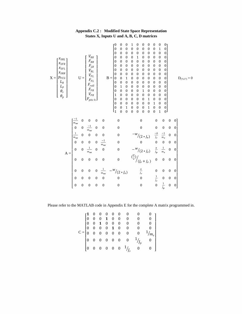
Appendix C.2 : Modified State Space Representation

States X, Inputs U and A, B, C, D matrices

X =

𝑥𝑆𝑅𝐿

𝑥𝑆𝐹𝑅

𝑥𝑆𝐹𝐿

𝑥𝑆𝑅𝑅

𝑝𝑉𝐶𝐺

𝐿𝑅

𝐿𝑃

𝜃𝑟

𝜃𝑝

U =

𝑉𝑅𝑅

𝐹𝑅𝑅

𝐹𝐿𝑅

𝑉𝑅𝐿

𝑉𝐹𝐿

𝐹𝐹𝐿

𝐹𝑟𝑜𝑙𝑙

𝐹𝐹𝑅

𝑉𝐹𝑅

𝐹𝑝𝑖𝑡𝑐 ℎ

B =

0 0 0 1 0 0 0 0 0 00 0 0 0 0 0 0 0 1 00 0 0 0 0 0 0 0 0 00 0 0 0 1 0 0 0 0 00 0 0 0 0 0 0 0 0 00 0 0 0 0 0 0 0 0 00 0 0 0 0 0 0 0 0 00 0 0 0 0 0 0 0 0 00 0 1 0 0 0 0 0 0 00 0 0 0 0 0 0 0 0 00 1 0 0 0 0 0 0 0 00 0 0 0 0 1 0 0 0 01 0 0 0 0 0 0 0 0 00 0 0 0 0 0 1 0 0 00 0 0 0 0 0 0 1 0 00 0 1 0 0 0 1 0 0 01 0 0 0 0 0 0 0 1 0

D(7x17) = 0

A =

−1

𝑚𝒖𝒔0 0 0 0 0 0 0 0 0 0

0 0−1

𝑚𝒖𝒔0 0 0 0 0 0 0 0

1

𝑚𝒖𝒔0 0 0 0 0 −𝑤

(2 ∗ 𝐽𝒓) −𝑏

𝐽𝒓

−1

𝑚𝒔0 0

0 0 0 0−1

𝑚𝒖𝒔0 0 0 0 0 0

0 01

𝑚𝒖𝒔0 0 0 −𝑤

(2 ∗ 𝐽𝒓) 𝑎

𝐽𝒑

1

𝑚𝒔0 0

0 0 0 0 0 0(𝑤

2)

(𝐽𝒓 + 𝐽𝒓 ) 0 0 0 0

0 0 0 01

𝑚𝒖𝒔−𝑤

(2 ∗ 𝐽𝒓) 𝑎

𝐽𝒓0 0 0 0

0 0 0 0 0 0 01

𝐽𝒓0 0 0

0 0 0 0 0 0 0 01

𝐽𝒑0 0

Please refer to the MATLAB code in Appendix E for the complete A matrix programmed in.

C =

𝟏 0 0 0 0 0 0 0 00 0 0 𝟏 0 0 0 0 00 0 𝟏 0 0 0 0 0 00 0 0 0 𝟏 0 0 0 0

0 0 0 0 0 0 0 0 1𝑚𝑠

0 0 0 0 0 0 0 1𝐽𝑝

0

0 0 0 0 0 0 1𝐽𝑟

0 0

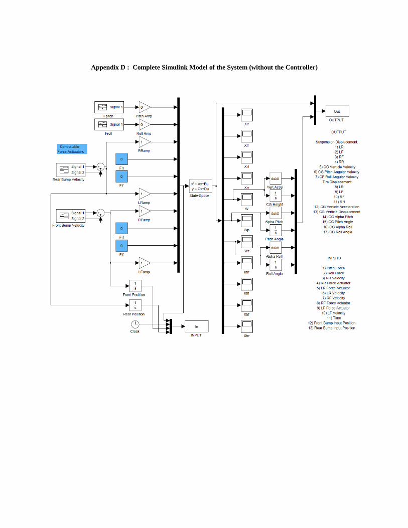
Appendix D : Complete Simulink Model of the System (without the Controller)

Appendix E : Complete Simulink Model with LQR Controller

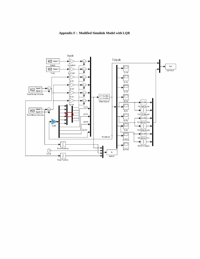
Appendix F : Modified Simulink Model with LQR

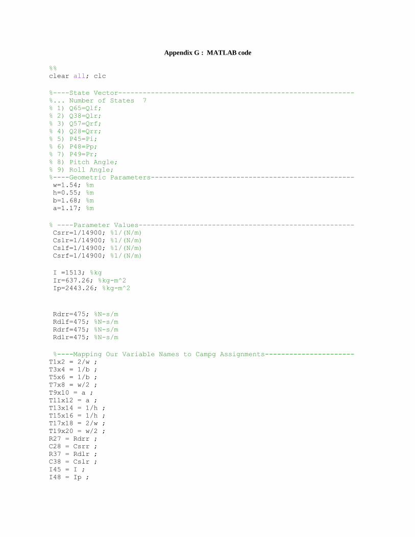
Appendix G : MATLAB code

%% clear all; clc

%----State Vector---------------------------------------------------------- %... Number of States 7 % 1) Q65=Qlf; % 2) Q38=Qlr; % 3) Q57=Qrf; % 4) Q28=Qrr; % 5) P45=Pi; % 6) P48=Pp; % 7) P49=Pr; % 8) Pitch Angle; % 9) Roll Angle; %----Geometric Parameters-------------------------------------------------- w=1.54; %m h=0.55; %m b=1.68; %m a=1.17; %m

% ----Parameter Values----------------------------------------------------- Csrr=1/14900; %1/(N/m) Cslr=1/14900; %1/(N/m) Cslf=1/14900; %1/(N/m) Csrf=1/14900; %1/(N/m)

I =1513; %kg Ir=637.26; %kg-m^2 Ip=2443.26; %kg-m^2

Rdrr=475; %N-s/m Rdlf=475; %N-s/m Rdrf=475; %N-s/m Rdlr=475; %N-s/m

%----Mapping Our Variable Names to Campg Assignments---------------------- T1x2 = 2/w ; T3x4 = 1/b ; T5x6 = 1/b ; T7x8 = w/2 ; T9x10 = a ; T11x12 = a ; T13x14 = 1/h ; T15x16 = 1/h ; T17x18 = 2/w ; T19x20 = w/2 ; R27 = Rdrr ; C28 = Csrr ; R37 = Rdlr ; C38 = Cslr ; I45 = I ; I48 = Ip ;

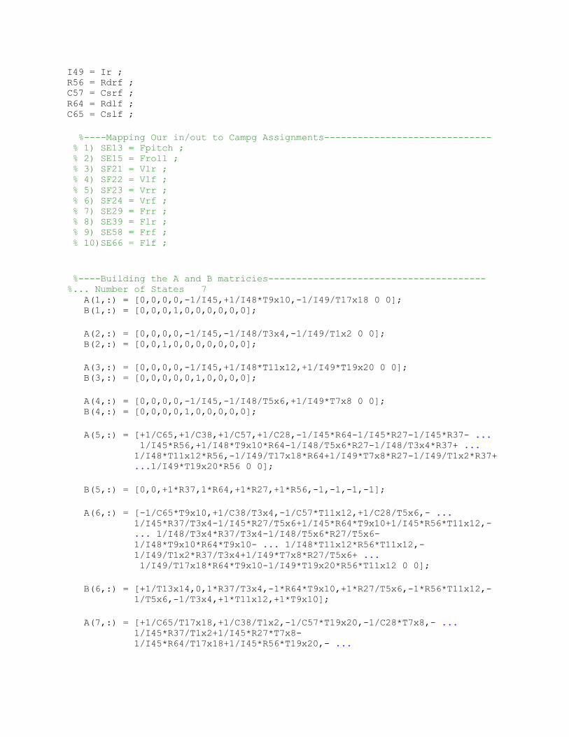
I49 = Ir ; R56 = Rdrf ; C57 = Csrf ; R64 = Rdlf ; C65 = Cslf ;

%----Mapping Our in/out to Campg Assignments------------------------------ % 1) SE13 = Fpitch ; % 2) SE15 = Froll ; % 3) SF21 = Vlr ; % 4) SF22 = Vlf ; % 5) SF23 = Vrr ; % 6) SF24 = Vrf ; % 7) SE29 = Frr ; % 8) SE39 = Flr ; % 9) SE58 = Frf ; % 10)SE66 = Flf ;

%----Building the A and B matricies--------------------------------------- %... Number of States 7 A(1,:) = [0,0,0,0,-1/I45,+1/I48*T9x10,-1/I49/T17x18 0 0]; B(1,:) = [0,0,0,1,0,0,0,0,0,0];

A(2,:) = [0,0,0,0,-1/I45,-1/I48/T3x4,-1/I49/T1x2 0 0]; B(2,:) = [0,0,1,0,0,0,0,0,0,0];

A(3,:) = [0,0,0,0,-1/I45,+1/I48*T11x12,+1/I49*T19x20 0 0]; B(3,:) = [0,0,0,0,0,1,0,0,0,0];

A(4,:) = [0,0,0,0,-1/I45,-1/I48/T5x6,+1/I49*T7x8 0 0]; B(4,:) = [0,0,0,0,1,0,0,0,0,0];

A(5,:) = [+1/C65,+1/C38,+1/C57,+1/C28,-1/I45*R64-1/I45*R27-1/I45*R37- ... 1/I45*R56,+1/I48*T9x10*R64-1/I48/T5x6*R27-1/I48/T3x4*R37+ ...

1/I48*T11x12*R56,-1/I49/T17x18*R64+1/I49*T7x8*R27-1/I49/T1x2*R37+

...1/I49*T19x20*R56 0 0];

B(5,:) = [0,0,+1*R37,1*R64,+1*R27,+1*R56,-1,-1,-1,-1];

A(6,:) = [-1/C65*T9x10,+1/C38/T3x4,-1/C57*T11x12,+1/C28/T5x6,- ...

1/I45*R37/T3x4-1/I45*R27/T5x6+1/I45*R64*T9x10+1/I45*R56*T11x12,-

... 1/I48/T3x4*R37/T3x4-1/I48/T5x6*R27/T5x6-

1/I48*T9x10*R64*T9x10- ... 1/I48*T11x12*R56*T11x12,-

1/I49/T1x2*R37/T3x4+1/I49*T7x8*R27/T5x6+ ... 1/I49/T17x18*R64*T9x10-1/I49*T19x20*R56*T11x12 0 0];

B(6,:) = [+1/T13x14,0,1*R37/T3x4,-1*R64*T9x10,+1*R27/T5x6,-1*R56*T11x12,-

1/T5x6,-1/T3x4,+1*T11x12,+1*T9x10];

A(7,:) = [+1/C65/T17x18,+1/C38/T1x2,-1/C57*T19x20,-1/C28*T7x8,- ...

1/I45*R37/T1x2+1/I45*R27*T7x8-

1/I45*R64/T17x18+1/I45*R56*T19x20,- ...

1/I48/T3x4*R37/T1x2+1/I48/T5x6*R27*T7x8+1/I48*T9x10*R64/T17x18-

... 1/I48*T11x12*R56*T19x20,-1/I49/T1x2*R37/T1x2-

1/I49*T7x8*R27*T7x8- ... 1/I49/T17x18*R64/T17x18-1/I49*T19x20*R56*T19x20 0 0];

B(7,:) = [0,+1/T15x16,1*R37/T1x2,+1*R64/T17x18,-1*R27*T7x8,-1*R56*T19x20,+ 1*T7x8,-1/T1x2,+1*T19x20,-1/T17x18];

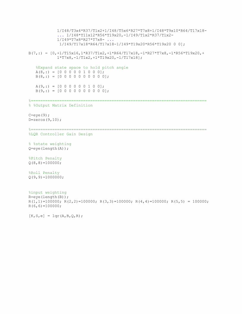
%Expand state space to hold pitch angle A(8,:) = [0 0 0 0 0 1 0 0 0]; B(8,:) = [0 0 0 0 0 0 0 0 0 0];

A(9,:) = [0 0 0 0 0 0 1 0 0]; B(9,:) = [0 0 0 0 0 0 0 0 0 0];

%========================================================================== % %Output Matrix Definition

C=eye(9); D=zeros(9,10);

%========================================================================== %LQR Controller Gain Design

% %state weighting Q=eye(length(A));

%Pitch Penalty Q(8,8)=100000;

%Roll Penalty Q(9,9)=1000000;

%input weighting R=eye(length(B)); R(1,1)=100000; R(2,2)=100000; R(3,3)=100000; R(4,4)=100000; R(5,5) = 100000;

R(6,6)=100000;

[K,S,e] = lqr(A,B,Q,R);