Embed Size (px)
Citation preview
VEHICLE SIZE CHOICE AND AUTOMOBILE EXTERNALITIES:
A DYNAMIC ANALYSIS
Clifford Winston Jia Yan
Brookings Institution Washington State University
Abstract. We study the effect of highway congestion on the “arms race” on American roads, which
has led to larger and more powerful vehicles that reduce safety and increase fuel consumption. We
estimate a dynamic vehicle size choice and replacement model and find that congestion delays
affect vehicle sizes. We then show that by addressing complementary externalities—congestion
and the externalities associated with larger vehicle sizes—congestion pricing could reduce the
vehicle fatality rate, generating $25 billion in annual benefits, and could improve vehicle fleet fuel
efficiency, generating roughly $10 billion in annual operating cost savings.
February 2018
1
1. Introduction
The internal combustion engine has been continuously refined since its introduction,
enabling motorists to trade off increasingly greater horsepower and fuel efficiency. Knittel (2011)
has shown that since the 1980s, motorists have revealed a strong preference for power as the
average horsepower of new passenger cars increased by 80 percent from 1980-2004, while fuel
economy increased by less than 6.5 percent, and average curb weight increased by 12 percent.
That preference has been underscored by the shift from passenger cars to light trucks and SUVs—
in 1980, 20 percent of new vehicles sold in the United States were light trucks and SUVs; in 2017,
that percentage climbed to 62 percent. The increasing power and weight of passenger vehicles is
all the more striking because it has occurred despite stricter emissions and fuel economy standards
that have created incentives for automobile companies to make lighter vehicles to reduce fuel
consumption and to get better fuel economy.1
Households’ preferences for larger more powerful vehicles have undoubtedly been
influenced by economic conditions, such as declining real gasoline prices during much of the
period. However, another potentially important factor that has been overlooked is the significant
growth of traffic congestion and delays on the nation’s highways. According to the Texas
Transportation Institute’s Urban Mobility Report, average annual traffic delays in U.S. urban areas
have increased from 18 hours in 1982 to 42 hours in 2014. As traffic congestion has increased and
1 Under the old fuel economy standards, which required each manufacturer to achieve a minimum
average MPG, manufacturers would have had to sell enough additional small vehicles to offset the
increased demand for larger vehicles. Under the new standards, which require each manufacturer
to achieve a minimum sales weighted average of the MPG targets for vehicles of each size that it
produces, manufacturers have to sell more smaller vehicles in a size class to offset the increased
demand for larger vehicles in that class.
2
trips have become more stressful, it is plausible that travelers have tried to increase their safety,
comfort, and privacy by driving larger and more powerful vehicles.2
Popular writers have illuminated motorists’ thought processes that led to the popularity of
SUVs: SUV buyers thought of big, heavy vehicles as safe; they found comfort in being surrounded
by so much rubber and steel (Gladwell (2004)). At the same time, the sheer size and menacing
appearance of SUVs inevitably made owners of other vehicles feel less safe. The result has been a
highway arms race (Bradsher (2002)).
White (2004) and Li (2012) reported empirical evidence that larger, heavier, and taller vehicles
provide better safety protection to occupants involved in a collision than smaller, lighter, and
shorter vehicles do, and that, all else constant, motorists are willing to pay a premium for vehicles
with those safety attributes, especially if much of their driving occurs in congested conditions
where they have a greater likelihood of being involved in an accident (Yeo, Jang, and Skabardonis
(2010)).3
2 Motorists place a greater value on the maneuverability of smaller vehicles on local streets and in
shopping areas than on urban highways. And although larger vehicles are less maneuverable than
smaller vehicles, which makes it more difficult for a driver of those vehicles to avoid a potential
accident, larger vehicles have a higher eye height, which gives a driver more sight distance and a
longer reaction time to avoid a potential accident. 3As pointed out by Ossiander, Koepsell, and McKnight (2014), the fatality risk of a vehicle is
determined by the crashworthiness of the vehicle (its ability to protect its own occupants), and the
crash aggressiveness of the vehicle (the hazard it imposes on the other vehicle in the crash). Before
1995, nearly all SUV models were built with a body-on-frame design, where the body was bolted
onto a strong ladder-type frame, as compared with a unibody design, where the body and frame
were designed and welded together as a single unit. Ossiander, Koepsell, and McKnight find that
the significant increase in SUVs since 1995 that are built with a unibody design has increased the
crashworthiness of SUVs and reduced their crash aggressiveness, although car occupants involved
in a two-vehicle crash are still more likely to be killed in a crash with an SUV than with another
car.
3
A valid causal relationship between highway congestion and vehicle size would indicate
that the major automobile externalities are positively related—that is, they are complementary
externalities—because larger vehicles: (1) consume more fuel than smaller vehicles and generally
produce greater emissions, and (2) increase the risk of a fatality to occupants of smaller vehicles
in a multi-vehicle crash (White (2004) and Anderson and Auffhammer (2014)), although in a
single-vehicle accident, larger vehicles may decrease the risk of a fatality to occupant. 4
Importantly, it is plausible that the marginal benefits of a tax on negative complementary
externalities are greater than the marginal benefits of a tax on negative non-complementary
externalities. Thus, a policy that reduces highway congestion, such as road pricing, could provide
significant additional social benefits, which have been overlooked in previous assessments, by also
reducing vehicle sizes and improving automobile safety and fuel economy.
The purpose of this paper is to conduct, to the best of our knowledge, the first disaggregate
analysis of the direct effect of highway congestion on vehicle size choice, controlling for other
important influences, including vehicle purchase price and operating costs, and to simulate the
effects of congestion pricing on vehicle fatalities and fuel economy.5 In theory, the gasoline tax,
4It could be argued that light trucks and SUVs increase highway congestion by requiring greater
road space. However, highway engineers measure both traffic volume and highway capacity in
terms of passenger car equivalents (PCEs) and they have not designated higher PCEs for light
trucks and SUVs as they have done for heavy trucks. In addition, significant improvements in
engine technology over time have enabled light trucks and SUVs to accelerate and decelerate much
faster, which reduces any particular disturbances that those vehicles may have on traffic flows.
The risk profiles of the type of drivers who self-select to purchase light trucks and SUVs may also
affect traffic flows and congestion if drivers of those vehicles are excessively risky or cautious.
But a definitive analysis of this issue requires complete information about drivers, their vehicles,
and their trips, which are formidable data requirements. Jacobsen (2013) and Makuch (2015) reach
conflicting conclusions about drivers’ riskiness by vehicle type; richer data is required to resolve
this issue.
5 Studies of the effect of residential density, which is likely to be correlated with greater highway
congestion, on vehicle use have obtained conflicting findings. Brownstone and Golob (2009)

4
which is currently used to simultaneously address all automobile externalities, has the greatest
impact on motorists who are committed to driving the most fuel inefficient vehicles (Langer,
Maheshri, and Winston (2017)); thus, it should discourage motorists from purchasing larger and
heavier light trucks and SUVs. But this effect has been blunted because: (1) Congress has
maintained the federal gasoline tax at its 1993 level of 18.4 cents per gallon, (2) real gasoline prices
have declined throughout much of the past few decades and are well below their highest levels
during the current decade, and (3) technological change has enabled larger vehicles to get better
fuel economy.
It is well known that congestion pricing could do a better job than the gasoline tax at reducing
peak-period congestion and guiding efficient investment in highway capacity (Lindsey (2012),
Winston (2013)), but its effect on reducing vehicle sizes and their concomitant externalities has
not been documented. We estimate that an efficient congestion charge would reduce the market
share of mid to full-size SUVs from about 31 percent to 23 percent and that it would reduce average
vehicle weight from 3860 pounds to 3730 pounds, which would result in: (1) a 10 percent decline
in the vehicle fatality rate that amounts to nearly $25 billion in annual nationwide benefits based
on conventional values of life, and (2) a 3 percent improvement in the average fuel efficiency of
the nation’s vehicle fleet which, holding VMT constant, reduces fuel consumption that amounts to
nearly $10 billion in annual operating cost savings.
Highway congestion and the economic factors and technological advance that have
contributed to households’ growing preference for power over fuel economy are unlikely to abate
found that greater residential density reduced fleet fuel efficiency through the choice of less fuel-
efficient vehicle types, while Brownstone and Fang (2014) found that an increase in residential
density had a negligible effect on car choice and utilization and slightly reduced truck choice and
utilization.
5
in the near future. At the same time, policymakers continue to resist widespread implementation
of congestion pricing. Thus, the potential ability of congestion pricing to simultaneously reduce
congestion and to efficiently encourage households to reduce their vehicle sizes, which would
generate additional benefits that would be widely shared among the public, should hopefully
improve its political appeal.
2. An Overview of the Sample
Our sample is based on data collected by GfK, a market research firm, on Seattle motorists
from 2004 to 2009. We chose Seattle for our geographic unit of analysis because it is a congested
metropolitan area with several bottlenecks created by bridges, and because NAVTEQ
(subsequently acquired by Nokia) could provide detailed real-time traffic data for its road network
during our period of analysis.
GfK provided a questionnaire to automobile commuters who are members of its survey panel
that asked them to indicate the roads that comprise the route that they use to get to work the
majority of the time. If another mode, such as a ferry was involved, only the auto portion of the
commute was included. Interstate freeways and state routes were identified by their number and
direction. Respondents also indicated: (1) the normal departure and arrival time of their commute,
(2) any regular stops that they make, (3) whether a High-Occupancy-Vehicle (HOV) lane is used
on the freeway portion of the commute, and (4) the vehicle that they normally use for the commute,
or for multi-vehicle households the two vehicles that they use if they are consistently alternated.
Any changes in the routes and departure and arrival times during the sample period were also noted.
We focus on the congestion delay that commuters experience on the freeway portion of their
commute because that delay is likely to be greater and more onerous than the delay on local roads

6
and arterials and thus more likely to influence their vehicle size choice. Such delay can be
measured accurately and addressed efficiently with public policies like congestion pricing without
disrupting a motorist’s journey, whereas congestion delay on local roads and arterials is more
difficult to measure accurately and is likely to be addressed less efficiently with a “toll ring” that
does not vary tolls in response to changes in traffic volumes throughout the day. Roughly 67% of
the commuting trips in our sample involved freeway travel. On average, 13% of freeway travel
time consisted of delays, and only 2% of non-freeway travel time consisted of delays, which
suggests that non-freeway travel delays are not important for our purposes. We later conduct a
robustness check by including only trips involving freeway travel in the estimation.
To obtain a respondent’s commuting information for each year, we used Traffic Message
Channel (TMC) codes for the Seattle Metropolitan Urban Area to identify the freeway segments
of the commute. We then used data from NAVTEQ to determine the average speeds and commute
times on those segments and summed them to obtain the average travel time for the entire freeway
portion of the commute.6 Congestion delays are therefore the difference between those average
travel times and commuters’ free flow travel times, which were based on the travel time of the
freeway portion of their commutes at 2am.
We show in figure 1 the distribution of the percentage of congestion delay in motorists’
commute time during our sample period. (The distribution changed very little from year to year.)
Some commuters experienced little delay but nearly half experienced non-trivial delays that
accounted for roughly 15% or more of the total time of the commute and about one-quarter
6 NAVTEQ reported their travel time data in “waves,” where travel times on a given segment were
based on a few years of data that were weighted toward the most recent year. For example, travel
time on a segment in 2006 was based on travel times from January 2004 to December 2006 that
were weighted toward 2006.
7
experienced sizable delays that accounted for roughly one-third or more of the total time of the
commute.7 Our base case specification of congestion delay attempted to capture the effect of those
delays on commuters’ vehicle size choice behavior, so we interacted a long commute dummy
variable, which indicates a commute that takes one hour or more, with an excessive delay dummy
variable, which indicates a level of congestion delay on the freeway portion of the commute that
accounts for 15% or more of the total time of the commute. We conducted a robustness check by
defining the excessive delay dummy variable to indicate congestion delay that accounts for 20%
or more of the total time of the commute.
In addition to obtaining information about the respondent’s automobile commute, the GfK
survey contained information on the respondents’ socioeconomic characteristics, including
household income, household size, age, gender, and education, and their zip code and housing
characteristics from which we determined the square footage of the house and the zip code’s Zillow
Home Value Index, median household income, school quality index, personal crime index, and
property crime index. The information on housing and residential location characteristics is
important for our identification strategy discussed later.
Final Sample
After eliminating respondents with missing information about their commute and location, we
obtained complete information from GfK for 271 respondents. We had to remove 41 of those
respondents from the sample because they had lived in the Seattle metropolitan area for only one
year while the dynamic choice model that we estimate requires an initial condition for each
7 Seattle motorists’ exposure to congestion is aligned with other urban motorists’ exposure to
congestion. We found that the estimates that we obtained using NAVTEQ’s data on the share of
driving time that Seattle commuters spend in congestion were comparable to estimates of that share
for drivers in other highly congested U.S. urban areas based on the Inrix Global Traffic Scorecard.

8
motorist and at least one subsequent holding and replacement choice. Thus our final sample
contained 230 respondents and 866 observations during 2004-2009. All of the respondents lived
in the Seattle Metropolitan Area and commuted to work by car as of 2009, although some did not
reside in Seattle for the entire 2004-2009 sample period. Roughly one-third of the respondents
switched vehicles in our sample, but we could not discern that, in general, those motorists switched
to larger (or smaller) vehicles. In addition, none of the respondents moved to a different residential
location.
The Seattle Metropolitan Area is adjacent to several bodies of water. The largest, Lake
Washington, separates downtown Seattle from some of its most populous suburbs. Many
commuters must travel over a body of water to get to their workplaces. The bridges that people
must cross when they drive into Seattle create many bottlenecks that significantly contribute to
congestion in the area. Figures 2a (North of Seattle Tacoma airport) and 2b (South of Seattle
Tacoma airport) indicate the residential locations of the commuters in our sample (blue dots) and
the major bottlenecks in the road network (black dots), as characterized by the Washington State
Department of Transportation.
The figures illustrate that the congestion and delays faced by Seattle commuters are the
outcome of their residential location choices (as well as their workplace choices), which expose
them or limit their exposure to bottlenecks. The considerable variation in delay that commuters in
our sample experience was shown in figure 1. Figures 2a and 2b also preview an important
identification issue that we address later—specifically, congestion may be correlated with
individuals’ unobserved characteristics that affect both their vehicle-size and residential location
choices.
9
Vehicle Size Choice Set and Vehicle Attributes
Consistent with the U.S. Department of Transportation, National Highway Transportation and
Safety Administration (NHTSA) classifications, we combined automakers’ vehicle classes and
sizes to define a product in our choice set, and we allowed motorists to select new vehicles and
used vehicles. The 13 vehicle size and class combinations in our choice set include:
1. Compact domestic;
2. Compact imported;
3. Compact pickup;
4. Full size SUV;
5. Full size domestic;
6. Full size imported;
7. Midsize SUV;
8. Midsize domestic;
9. Midsize imported;
10. Passenger van;
11. Standard pickup;
12. Sub-compact domestic; and
13. Sub-compact imported.
When motorists decide to replace their current vehicles, we assume they choose among
vehicle class and size combination from the most recent 10 model years. Thus, in a given year, a
motorist’s choice set consists of 130 alternatives.
We used data from Ward’s Automotive Yearbook, various editions, to construct vehicle
attributes, including purchase price, miles-per-gallon (mpg), body-weight, and horsepower, for
10
each choice alternative by averaging those attributes across vehicles for each combination of
vehicle class, size, and model year.8 We then measured the operating cost (in dollars per mile) for
those combinations as the ratio of the average gasoline price in Seattle to the average miles per
gallon on both highways and local roads. Finally, we obtained vehicle registration data from R.L.
Polk, Incorporated to construct the population shares in Seattle of each vehicle class and size
combination during the sample period.
We compare the population shares and the sample shares of the vehicle class and size
combinations in table 1. Generally, the population and sample shares suggest that the pronounced
shift to larger vehicles that occurred in the preceding decades has abated to some extent, perhaps
because the period of our analysis includes the Great Recession that began in 2007 and ended in
2009. In any case, midsize luxury vehicles and midsize SUVs comprise the largest vehicle shares
in the population and in our sample, although the share of midsize luxury vehicles is somewhat
larger in our sample than in the population. Most of the other population and sample shares of the
vehicle class and size combinations are aligned, with the exceptions that the population share of
compact pickups is larger than the sample share and the sample share of full size SUVs is larger
than the population share. The difference in some of the population and sample shares motivate
us to perform a robustness check of our findings by re-estimating our base case model by Weighted
Exogenous Sample Maximum Likelihood (WESML) to align the sample and population shares of
all the vehicle class and size combinations.
We summarize the motorists’ socioeconomic and demographic variables in our analysis in
table 2. It is interesting that the average household income of automobile commuters in our sample
8 We accounted for vehicle depreciation when we constructed the purchase prices for used vehicles.
We did not find that the variance of vehicle attributes varied greatly across the vehicle size classes
that we used.
11
is more than double the median city household income, which also includes public transit
commuters who tend to have lower incomes than automobile commuters. In addition, nearly two-
thirds of the motorists in our sample have a long commute that exceeds one hour. Based on U.S.
Census data, it could be argued that Seattle’s inflated housing market and its high cost of living
has caused younger people to get started on owning a home by buying one that is far from their
workplace and then commuting long distances to jobs that help them afford their mortgage
payments. We also stress that our sample consists only of people who are employed and who are
more likely than unemployed people to own a home in the outlying suburbs that is not close to
their workplace.
The vehicle attributes that we summarize in table 3 are consistent with the tradeoff that
motorists have made since the 1980s of driving vehicles with greater horsepower (and body weight)
while not improving fuel economy (Knittel (2011)).
3. A Dynamic Model of Vehicle Holdings and Replacement
Our sample enables us to identify motorists’ preferences for vehicle attributes, including
purchase price, operating cost, weight, horsepower, and vehicle size, when they face different
levels of congestion and in two decisionmaking environments: (1) the decision of whether to keep
or replace a vehicle, and (2) the decision of which vehicle to purchase when they decide to replace
a vehicle.
Dynamic models have been developed to analyze automobile purchase decisions because
automobiles are a durable good and because brand loyalty based on a motorist’s accumulated
experience with owning a particular vehicle make is likely to influence future purchase decisions
(Mannering and Winston (1985)). However, brand loyalty is unlikely to be an important
12
consideration in our analysis of vehicle size choice, which does not distinguish between
automakers, but it is still appropriate for us to develop a dynamic model to estimate vehicle holding
and replacement decisions because:
● Motorists do not change their vehicles frequently and when they do, they generally sell a
vehicle that they currently own in the used-vehicle market and incur transactions costs.
● As a vehicle that a motorist owns ages, its price depreciates and its maintenance costs
increase.
● Vehicle operating costs evolve over time with the fluctuation in gasoline prices and
motorists have expectations about those prices that may influence vehicle decisions.
● Technological advance in the automobile industry causes vehicle attributes to improve over
time.
Our disaggregated data set enables us to account for those considerations and to estimate a
dynamic model of vehicle size choice and replacement. We note that it would be very difficult to
formulate and estimate such a dynamic model using aggregated data.
Model Assumptions
Many studies of motorists’ preferences for vehicle attributes analyze the one-period utility
maximizing decision to purchase a new vehicle from the available makes and models on the market
(for example, Train and Winston (2007)). The major challenge to analyze vehicle choice behavior
in a dynamic context is the large-dimension of the state space. Schiraldi (2011) employs the
Inclusive Value Sufficiency (IVS) assumption, formalized by Gowrisankaran and Rysman (2012)
in a study of the demand for camcorders, to reduce the dimensionality in their multinomial logit
model of motorists’ vehicle choice. They formulate that model in the context of a dynamic optimal
stopping problem. Under the IVS assumption, all states that lead to the same inclusive value,
13
which measures a decisonmaker’s ex-ante present discounted value of purchasing the preferred
vehicle instead of holding on to the current vehicle, are equivalent. Thus, the decisionmaker tracks
only the inclusive value instead of the relevant vehicle attributes. Although the assumption
simplifies the analysis, it is purely mathematical and has little behavioral justification. This
drawback is particularly relevant here because we use disaggregated data and we therefore need
information about the state that each motorist faces when making replacement and purchase
decisions.
We develop a tractable dynamic choice model by making plausible assumptions, which have
clear behavioral interpretations, based on the relevant features of the automobile industry and the
available empirical evidence in the literature.
Assumption 1: Consumers do not predict the evolution of the automobile industry’s vehicle
offerings.
This assumption is plausible because most consumers do not frequently change their vehicles;
thus, they pay close attention to the vehicle market only periodically. 9 At the same time,
automakers do not significantly change vehicle designs frequently so vehicle attributes tend to be
stable for several years. In our model, we construct average attributes based on combining
individual vehicles into combinations of class, size, and year, which will be even more stable over
time than individual vehicles’ attributes. The implication of this assumption is that consumers
assume that the same attributes in their current choice set, which we have noted, will be available
in their future choice sets.
9 This assumption is also likely to be plausible for consumers who lease their vehicles. Mannering,
Winston, and Sharkey (2002) found that high-income households are attracted to leasing because
it facilitates vehicle upgrading. Nonetheless, such households also follow the vehicle market
periodically because they lease their vehicles for a number of years.
14
Assumption 2: Motorists make reasonable predictions of gasoline prices and base their vehicle
replacement decisions on those predictions.
Anderson, Kellogg, and Sallee (2013) provide support for this assumption with empirical
evidence that indicates that consumers predict future gasoline prices based on current gasoline
prices and that they make vehicle purchase decisions based on that prediction.
Assumption 3: Consumers track over time the increasing maintenance costs of the vehicles they
currently own and the depreciation of their prices.
Given the notable changes in and available information about maintenance costs and resale
prices over time, it is plausible that consumers take account of those factors in their vehicle holding
and replacement decisions.
Assumption 4: Congestion on urban roads persists and exhibits stable growth in normal
macroeconomic environments, but motorists do not form expectations about future congestion
growth that affect their vehicle holding and replacement decisions.
Seattle is a mature urban area and, as noted, many motorists have long commutes and are
subject to congestion, especially if their commute involves a bottleneck. Given our focus on
excessive delay and the fact that congestion does not decrease in the long run, it is plausible that
motorists take their exposure to congestion as given when they made their residential location and
vehicle decisions.
Model Formulation
We model motorists’ vehicle holding and replacement decisions as an optimal stopping
problem. We index a sequence of observations for each motorist by year Tt ,...,1,0 , with a
motorist owning a vehicle in the initial period 0t . Given the initial vehicle holding in 2004, the
motorist decides whether to hold or to replace the vehicle with another one in each subsequent
year starting in 2005. In this dynamic model, identification of the effects of purchase price,
15
operating costs, and congestion on vehicle size choice relies on variation in both vehicle holdings
and replacement decisions over time and across motorists, given the initial holdings.
We summarize in figure 3 the information requirements and holdings and replacement
decisions in the dynamic model. In the initial year of our analysis, a motorist owns a vehicle and
has complete information on the attributes of all the vehicles in the market. The motorist’s
preferences for vehicles face random shocks in every period that are realized at the beginning of a
period. At the same time, the motorist receives information on gasoline prices and formulates
expectations of future gasoline prices. Given the information set, the motorist makes a decision
of whether to keep the current vehicle or to replace it with another one subject to the preceding
four assumptions. The decision generates a utility gain to the motorist in that period and affects
the individual’s utility in future periods by determining the state—the vehicle that the individual
owns—at the beginning of the next period.
Transition of States
Given assumptions 1-4, the information set or the state space of a motorist i , who owns a
vehicle j at the beginning of a period t , is ittjtijt gaj ,,, , where jta is the age of the vehicle
the motorist owns; tg is the price of gasoline; and
tCkiktit is the set of random shocks
affecting the motorist’s preference for vehicles contained in the choice set tC . The transition of
the uncontrolled states ittjtijt ga ,, is denoted by ijtijt 1 .
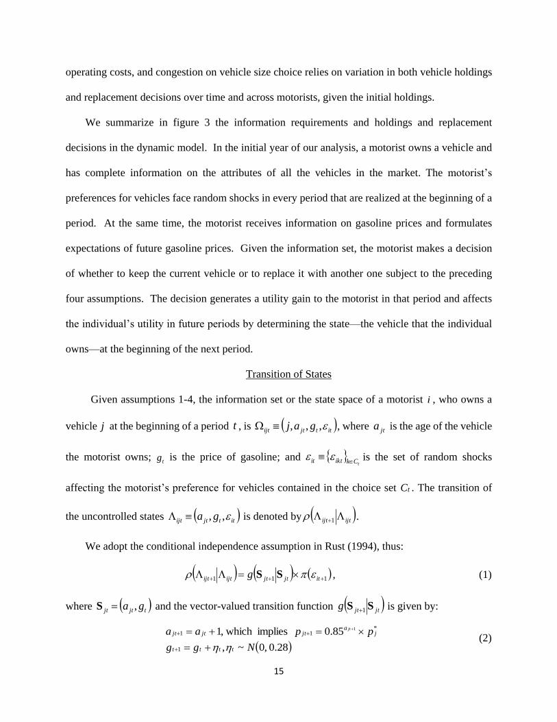
We adopt the conditional independence assumption in Rust (1994), thus:
111 itjtjtijtijt g SS , (1)
where tjtjt ga ,S and the vector-valued transition function jtjtg SS 1 is given by:
28.0 ,0~,
85.0 implies which ,1
1
*11
1
Ngg
ppaa
tttt
ja
jtjtjtjt
(2)

16
The first condition in equation (2) simply says that the age of the vehicle that the motorist owns is
increased by one in the next period; accordingly, the manufacturer’s price *
jp of vehicle j
depreciates with vehicle age at a rate of 15%, which is consistent with industry standards.10
Increases in vehicle age also capture the effects of other influences on vehicle size choice, such as
maintenance costs, which increase with vehicle age. The second condition indicates that the
evolution of the price of gasoline follows a normal random-walk process that is estimated from
data on average gasoline prices for U.S. cities from 1981 to 2014.11 Finally, we assume that the
distribution of the random shocks, 1it , is given by a multivariate extreme-value density.
One-period Utility and Accounting for Vehicle Price Endogeneity
The one-period indirect utility that motorist i obtains from keeping vehicle j in year t is
given by:
ijtitjijtijtitjjijtijt vu μVVBx , (3)
where jtx is a vector of vehicle attributes, including vehicle age, size, body-weight, purchase price,
and operating cost, which is determined by the price of gasoline and the vehicle’s fuel economy
(mpg); j captures omitted attributes of a vehicle in the spirit of Berry, Levinsohn, and Pakes
(BLP 1995) so we can avoid the bias caused by endogeneity of the vehicle’s purchase price.
Because we have disaggregated data on motorists’ vehicle choices over time and because we
focus on vehicle-size choice, we can use a fixed-effects specification to control for the omitted
10 https://www.carfax.com/guides/buying-used/what-to-consider/car-depreciation.
Heterogeneity in vehicle depreciation is less within a given vehicle size classification.
11 We conducted a Dickey-Fuller test and we could not reject the null hypothesis that gasoline
prices follow a random-walk process. Empirical evidence in Anderson, Kellogg, and Sallee (2013)
also indicates that consumers formulate their expectations of future gasoline prices based on a
random-walk process.
17
product attributes. Specifically, we specify j with dummy variables for the 13 vehicle class and
size combinations in our analysis, and we assume that the omitted attributes in a given class and
size combination for different model years are the same. This assumption is plausible because
vehicle manufacturers do not significantly change their vehicle designs frequently. In addition,
although new safety features may be introduced, they are introduced for a specific vehicle class or
classes so that all new vehicles in that class are equipped with those features during the same year
or possibly a year later. Compared with the random-effects BLP specification, which assumes that
j is correlated with the purchase price but uncorrelated with other observed attributes, the fixed-
effects specification that we use here has the advantage that it allows omitted vehicle attributes to
be correlated with observed vehicle attributes in a flexible way.
Finally, jV is a vector of four vehicle classification dummies (large vehicles, luxury vehicles,
SUVs, and new vehicles) and itμ a vector of normal random variables with zero mean—that is, it
forms a covariance matrix that we estimate. This specification mimics a nested-logit specification
in which different vehicle class and size combinations are grouped into four overlapped nests to
generate flexible substitution patterns among alternatives, thereby relaxing the restrictive IIA
assumption.
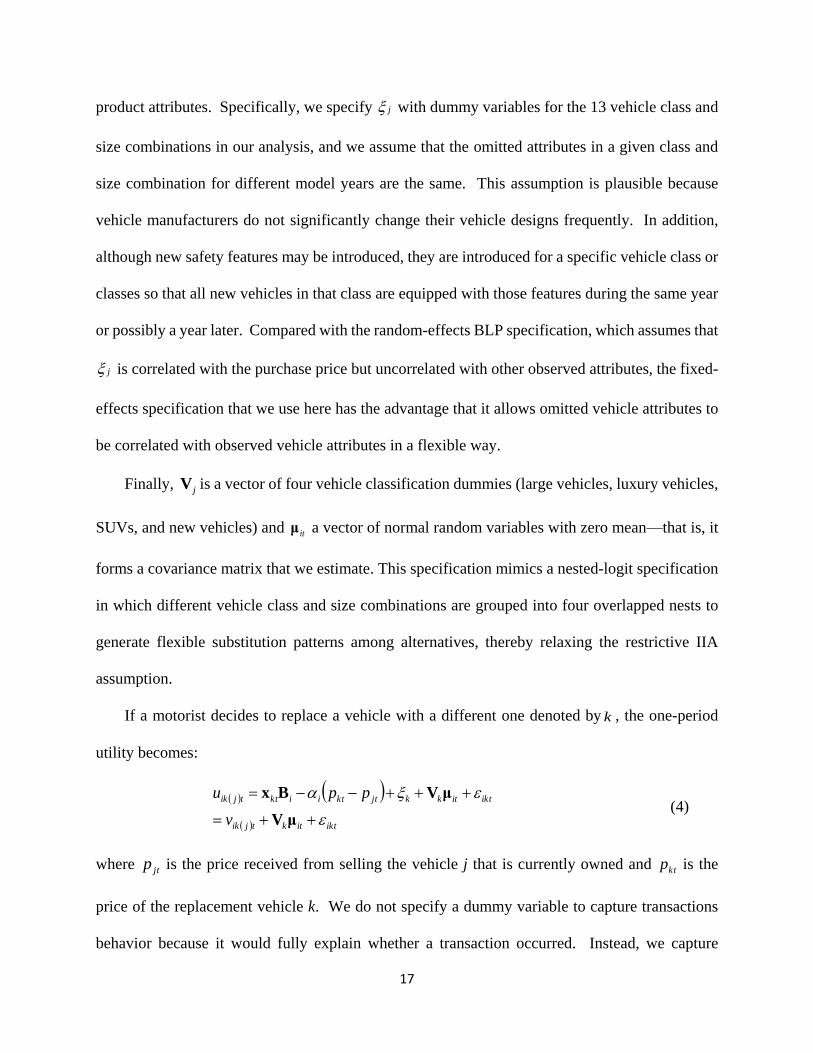
If a motorist decides to replace a vehicle with a different one denoted by k , the one-period
utility becomes:
iktitktjik
iktitkkjtktiikttjik
v
ppu
μV
μVBx (4)
where jtp is the price received from selling the vehicle j that is currently owned and ktp is the
price of the replacement vehicle k. We do not specify a dummy variable to capture transactions
behavior because it would fully explain whether a transaction occurred. Instead, we capture
18
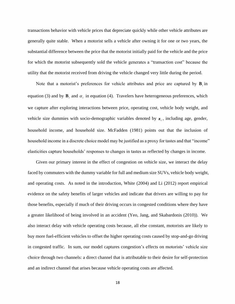
transactions behavior with vehicle prices that depreciate quickly while other vehicle attributes are
generally quite stable. When a motorist sells a vehicle after owning it for one or two years, the
substantial difference between the price that the motorist initially paid for the vehicle and the price
for which the motorist subsequently sold the vehicle generates a “transaction cost” because the
utility that the motorist received from driving the vehicle changed very little during the period.
Note that a motorist’s preferences for vehicle attributes and price are captured by iB in
equation (3) and by iB and i in equation (4). Travelers have heterogeneous preferences, which
we capture after exploring interactions between price, operating cost, vehicle body weight, and
vehicle size dummies with socio-demographic variables denoted by iz , including age, gender,
household income, and household size. McFadden (1981) points out that the inclusion of
household income in a discrete choice model may be justified as a proxy for tastes and that “income”
elasticities capture households’ responses to changes in tastes as reflected by changes in income.
Given our primary interest in the effect of congestion on vehicle size, we interact the delay
faced by commuters with the dummy variable for full and medium size SUVs, vehicle body weight,
and operating costs. As noted in the introduction, White (2004) and Li (2012) report empirical
evidence on the safety benefits of larger vehicles and indicate that drivers are willing to pay for
those benefits, especially if much of their driving occurs in congested conditions where they have
a greater likelihood of being involved in an accident (Yeo, Jang, and Skabardonis (2010)). We
also interact delay with vehicle operating costs because, all else constant, motorists are likely to
buy more fuel-efficient vehicles to offset the higher operating costs caused by stop-and-go driving
in congested traffic. In sum, our model captures congestion’s effects on motorists’ vehicle size
choice through two channels: a direct channel that is attributable to their desire for self-protection
and an indirect channel that arises because vehicle operating costs are affected.
19
Endogenous congestion
As suggested in figures 2a and 2b, motorists’ congestion delays are affected by their residential
location choices, which are affected by their preferences for both neighborhood and housing
attributes. At the same time, those preferences are likely to be correlated with their vehicle
preferences. To take some examples, a motorist who likes large vehicles may also like a spacious
house located in an expensive area; a motorist who likes a “trendy” vehicle may also like a cool
house in a “trendy” neighborhood; and a motorist who likes a luxury vehicle may also like a
stunning house in an exclusive neighborhood. In sum, motorists are likely to sort themselves into
different residential locations according to their preferences for housing and location attributes,
and because their preferences for vehicle attributes and for housing and location attributes are
correlated, motorists living in different locations have different vehicle preferences.
Our modeling approach attempts to identify the effect of congestion on motorists’ vehicle-size
choices through the variation in their choices under different commuting conditions, as reflected
in congestion delays. However, the estimated effect may reflect the heterogeneity in the vehicle
preferences of motorists who choose to live in different locations. Attempting to address this
problem by modeling residential location choice jointly with vehicle size choice is quite difficult
and, to the best of our knowledge, a dynamic disaggregate model of residential location choice
does not exist. A fundamental challenge is to accurately characterize the choice set over time,
including the non-chosen alternatives and their attributes, and even if that is possible, jointly
estimating both residential location choice and vehicle size choice in a dynamic framework is a
daunting task.12 Because we perform maximum likelihood estimation of a nonlinear model, there
12 Of course, there are many studies of the choice of residential location that use a zip-code as the
basic unit of analysis and even in a disaggregated analysis, zip-code demographic variables are
more likely to be controlled for than are individual demographic variables. Nonetheless, the

20
is no corresponding approach where we could use a plausible instrument for congestion, assuming
one exists in this context. Instead, we would have to develop a structural model of congestion and
derive the complete data likelihood, which is equivalent to jointly estimating vehicle size and
location choices.
Still another strategy to overcome the identification issue caused by endogenous congestion is
to treat iB as motorist fixed-effects, which are estimated in the dynamic choice model and capture
unobserved characteristics of motorists that lead to correlation of their vehicle and location
preferences. But the strategy of using motorist dummy variables faces the incidental parameter
problem (Lancaster (2000)), because the time series is short (2004-2009); iB cannot be estimated
precisely from at most six observations.
Thus our empirical strategy to achieve identification uses selection on observables, where we
specify as controls several variables that are well-known in the urban housing and location
literature (for example, McFadden (1978)) to affect location and housing choices to capture
unobserved preferences, including: (1) the size of the motorists’ houses measured by square feet,
and (2) several attributes of the location, measured at the zip code where the motorists live,
including the Zillow home value index, median household income, school quality index, personal
crime index, and property crime index.13 We pointed out that motorists sort themselves into
different residences according to their location and housing preferences, which are correlated with
challenge to estimate a joint dynamic model of vehicle size choice, replacement, and residential
location choice is formidable.
13 Our approach to reduce the potential bias caused by unobservables by controlling for several
observables is in the spirit of Altonji, Elder, and Taber (2005). However, we cannot use their
approach to test for a critical value where bias is unlikely because we estimate a nonlinear dynamic
model instead of a linear regression model.
21
their vehicle preferences. Our empirical strategy implicitly assumes that those observables
influence the sorting process so that motorists in locations with similar characteristics have similar
vehicle preferences holding congestion constant.
Let iw denote those control variables and
iβ denote the vector of coefficients of the SUVs,
vehicle body weight, and operating cost, which are a subset of the coefficients in iB . As before,
socioeconomic variables are denoted byiz , thus:
θδwγzβ iiii delay , (5)
and δw i in equation (5) captures the preference heterogeneity of motorists living in different
locations with different attributes and in different houses with different sizes, and θ captures the
net effect of delay on preferences for vehicle size, vehicle weight, and operating cost.
An important consideration that alleviates concern about the potential endogeneity of
congestion delay is that compared with vehicle size choice, location and housing decisions are
made over a much longer time horizon and households face greater constraints if they wish to
change those decisions. Given our panel data, motorists’ location and housing are likely to be pre-
determined, thereby enabling the time-invariant control variables in equation (5) to absorb the
effects of location choice on vehicle attributes. This is especially true because nearly 80 percent
of the motorists in our sample lived in Seattle for at least five years. When we estimated our model
on a sample that eliminated motorists who did not live in Seattle for at least five years, we found
that our main findings were not much affected, which also suggests that the sample households
have not significantly adjusted their vehicle preferences as they have become more familiar with
living in Seattle.
22
As noted, none of the motorists in our sample changed their locations during the period of
analysis, but one-third of the motorists changed their vehicle holdings.14 If households could
easily change locations to avoid congestion, then we would overestimate the effects of congestion
on vehicle size choice.
Motorists’ Forward-Looking Decision
Given the information set ijt and our characterization of the transition of states in equation
(2), motorists’ decide to keep or replace their current vehicle to maximize expected lifetime utility.
If a motorist keeps vehicle j instead of replacing it, the present value of the motorist’s maximal
utility in the planning horizon is given by:
jtitjtitijtitjtit jjEVujV SSS ,,,,,~
111 , (6)
where 1itEV denotes the expected value function and 1,0 is the discount factor.
To replace vehicle j with vehicle k, the motorist solves the following problem:
jtitktittjik
jkCk
itjtit jkEVuMaxjVt
SSS ,,,,,ˆ111
. (7)
Thus the individual keeps vehicle j in period t if and only if itjtititjtit jVjV ,,
~,,ˆ SS such that
the valuation-function satisfies the following Bellman equation:
itjtititjtititjtit jVjVMaxjV ,,ˆ,,,~
,, SSS . (8)
Because it contains a motorist’s private information, we integrate the preference shocks out of
equation (8) by defining motorist si' expected value of holding any vehicle type j in year t as:
14 The fact that our sample includes the Great Recession limits households’ mobility, but we also
include a number of years before the Recession.
23
ijtjtjtititjijt
itititjtitjtit
IjjWEv
djVjW
it
exp,,expln
,,,
11
SSμV
SS
(9)
jkCk
jtktititktjikijt
t
jkWEvI SSμV ,,expln 11 . (10)
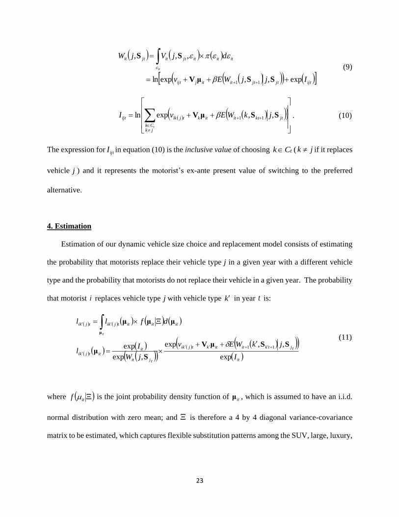
The expression for ijtI in equation (10) is the inclusive value of choosing tCk ( jk if it replaces
vehicle j ) and it represents the motorist’s ex-ante present value of switching to the preferred
alternative.
4. Estimation
Estimation of our dynamic vehicle size choice and replacement model consists of estimating
the probability that motorists replace their vehicle type j in a given year with a different vehicle
type and the probability that motorists do not replace their vehicle in a given year. The probability
that motorist i replaces vehicle type j with vehicle type k in year t is:
it
tjtkititktjki
tjit
itittjki
ititittjkitjki
I
jkWEv
jW
Il
dfll
it
exp
,,exp
,exp
exp 11 SSμV
Sμ
μμμ
μ
(11)
where itf is the joint probability density function of itμ , which is assumed to have an i.i.d.
normal distribution with zero mean; and is therefore a 4 by 4 diagonal variance-covariance
matrix to be estimated, which captures flexible substitution patterns among the SUV, large, luxury,
24
and new vehicle classifications. The probability that motorist i does not replace vehicle j in year t
is:
itit
tjit
itti df
jW
Il
it
μμS
μ
,exp
exp10 . (12)
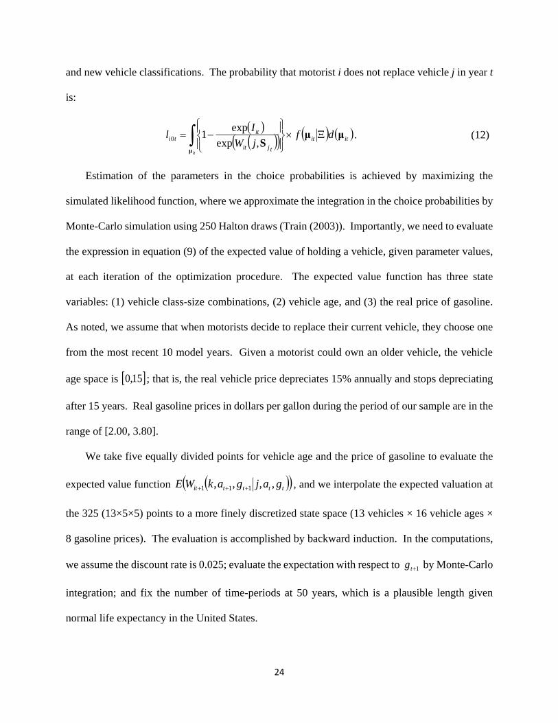
Estimation of the parameters in the choice probabilities is achieved by maximizing the
simulated likelihood function, where we approximate the integration in the choice probabilities by
Monte-Carlo simulation using 250 Halton draws (Train (2003)). Importantly, we need to evaluate
the expression in equation (9) of the expected value of holding a vehicle, given parameter values,
at each iteration of the optimization procedure. The expected value function has three state
variables: (1) vehicle class-size combinations, (2) vehicle age, and (3) the real price of gasoline.
As noted, we assume that when motorists decide to replace their current vehicle, they choose one
from the most recent 10 model years. Given a motorist could own an older vehicle, the vehicle
age space is 15,0 ; that is, the real vehicle price depreciates 15% annually and stops depreciating
after 15 years. Real gasoline prices in dollars per gallon during the period of our sample are in the
range of [2.00, 3.80].
We take five equally divided points for vehicle age and the price of gasoline to evaluate the
expected value function ttttit gajgakWE ,,,, 111 , and we interpolate the expected valuation at
the 325 (13×5×5) points to a more finely discretized state space (13 vehicles × 16 vehicle ages ×
8 gasoline prices). The evaluation is accomplished by backward induction. In the computations,
we assume the discount rate is 0.025; evaluate the expectation with respect to 1tg by Monte-Carlo
integration; and fix the number of time-periods at 50 years, which is a plausible length given
normal life expectancy in the United States.
25
We ensured that we achieved a global optimum of the simulated likelihood function by
varying the initial starting values of the parameters. Finally, we discuss the robustness of our
parameter estimates later, but we report here that our findings were not affected by our assumptions
about the discount rate and the number of time periods.15
5. Estimation Results
We estimated a basic specification for both the myopic and dynamic models, which included
the important interactions between congestion delays and vehicle characteristics, vehicle attributes,
observed and unobserved heterogeneity, and a full set of interactions with demographic variables
and housing and location characteristics. We then performed a series of robustness checks of our
findings on the effects of congestion delays on vehicle size choice and replacement.
Baseline Models
The estimated parameters of the myopic and dynamic choice models presented in table 4 are,
in general, statistically reliable and have plausible signs. Based on the greater value of its log-
likelihood, the dynamic model fits the data better than the myopic model does. The coefficients
of greatest interest capture the effect of interactions between congestion and vehicle characteristics
on vehicle size choice. We find that motorists are more likely to acquire a full or mid-size SUV,
a heavier vehicle, and a vehicle with lower operating costs as congestion delays increase, indicating
that congestion simultaneously affects—in a conflicting manner—motorists’ safety and fuel
15 We conducted sensitivity analyses of the dynamic baseline model by reducing the discount rate
by 50% and increasing the number of time periods to 75 years.
26
economy considerations.16 Motorists react more strongly—that is, they are more inclined to
purchase larger vehicles and to replace their vehicles more quickly—to congestion’s interactions
with vehicle characteristics in the dynamic model than in the myopic model because the reduction
in safety and fuel economy that is caused by congestion persists through time.
Similarly, an examination of the coefficients of the vehicle attributes indicates that motorists
place a greater value on reducing operating costs and less value on reducing the vehicle purchase
price in the dynamic model compared with their valuations of those attributes in the myopic model.
The purchase price represents motorists’ “set-up costs” while motorists incur operating costs in
every period. A static model cannot capture the different effects of those costs on motorists’
vehicle size and replacement decisions as accurately as a dynamic model can and thus it
overestimates the effect of the purchase price on those vehicle decisions. The effects of other
vehicle attributes, including horsepower (specified alone and divided by vehicle weight), a dummy
variable indicating a new or used vehicle, and a dummy variable indicating whether the age of the
vehicle exceeds five years, are similar for the dynamic and myopic models.
We capture observed heterogeneity in the specification by interacting household income per
capita with the vehicle purchase price, operating cost, and congestion delay. We also capture
preference heterogeneity that indicates that households with higher income per capita have a
greater preference for luxury vehicles than other households have and that larger households have
a greater preference for passenger vans than other households have. Those preferences are stronger
in the dynamic model than in the myopic model because household sizes and incomes often
16 We also estimated a model where we interacted congestion delays with a compact vehicle and
we found that motorists were less likely to acquire those vehicles as congestion increased, but the
estimated coefficient was statistically insignificant.
27
increase over time. Finally, we capture unobserved heterogeneity with random coefficients for the
large, luxury, SUV, and new vehicle dummy variables
Robustness Checks
We preformed several robustness checks to shed light on our identification strategy and to test
certain assumptions that we have made in the analysis. First, we focused on freeway delays and
we noted that non-freeway delays accounted for only a very small share of non-freeway travel time
in our sample of commutes. We tested whether the inclusion of commutes that do not involve
freeway travel affected our findings by estimating our baseline dynamic model with a sample that
included only commutes that involved freeway travel. In this subsample, freeway delays
accounted for 83% of total delays. As shown in the second column of table 5, our estimates of the
interactions involving delay are not affected much when we restrict our sample only to commutes
that involve freeway travel.
Second, we identified the effects of congestion delays on vehicle size and replacement choice
by including interactions between housing and residential location characteristics to control for
unobserved influences that may affect both location and vehicle size decisions and bias our
estimates of congestion’s effects. The third column of table 5 shows that removing those
interactions reduces the effects of congestion, especially through its interaction with operating cost;
thus, we avoided a potential downward bias in the parameter estimates of the congestion delay
interactions by including the housing and residential location characteristics.
Third, we discussed the assumptions that we used to measure congestion delays and we
pointed out that given the distribution of the percentage of delay in motorists’ commute time, we
could have set a higher threshold for excessive delay and still captured the effect of those delays
on motorists’ vehicle size choices. Thus, we re-estimated our dynamic choice model and we

28
assumed that the excessive delay dummy took on a value of 1 if congestion delay amounted to 20
percent, instead of 15 percent, or more of total commute time. The estimates in the fourth column
of table 5 indicate that the estimated effects of congestion on vehicle size are somewhat lower, but
not statistically significantly different from the estimated effects that we obtained under our initial
assumptions.
Finally, as an interpretative matter, it could be argued that we are capturing the effect of
commute distance instead of congestion on vehicle size choice. However, in our sample, the
correlation between commute distance and congestion, defined as the percentage of delay in total
commuting time, was only 0.28. Importantly, we show in table 6 that the estimates of the vehicle
size and operating cost interactions involving delay are not strongly affected when we also include
in the specification interactions between the commute distance and the vehicle size and operating
cost variables.
We provide additional perspective on our identification approach by splitting the sample to
limit households’ mobility and to reduce the endogeneity from commuters’ potential changes in
residential location. Table 7 presents estimation results for models where we split the sample
between commutes that are less than and greater than or equal to ten miles. We find that congestion
still affects vehicle size through its interactions with vehicle characteristics for the longer
commutes. However, we also find that congestion no longer affects vehicle size through its
interactions with SUVs and operating costs for the shorter commutes where, in all likelihood,
commuters’ considerations of the safety protection and fuel economy provided by vehicle size are
less important because the risk of an accident, which is partly determined by exposure in terms of
vehicle miles traveled (VMT), and total vehicle operating costs are lower.

29
In table 8, we present estimation results for models where we split the sample between
commuters from households with annual incomes less than and greater than or equal to $50,000.
Congestion affects the vehicle size choices of both groups of commuters, but the more affluent
commuters respond much more strongly to congestion’s interaction with SUVs and body weight,
perhaps because they have a higher value of life and place a greater premium on vehicle safety
characteristics. At the same time, they also respond more strongly to congestion’s interaction with
operating costs, in all likelihood to partially offset the higher operating costs they incur by driving
heavier and larger vehicles.
As noted, our analysis has proceeded under the assumption that our sample of Seattle
commuters is representative of the population of Seattle commuters. However, we pointed out in
table 1 that some of the shares of the 13 vehicle classifications in our sample were not closely
aligned with the shares in the population. We therefore tested whether this characteristic of our
sample had led to any bias by re-estimating our dynamic vehicle size choice model with a
WESMLE estimator that uses weights to align the sample shares of the 13 vehicle classifications
with the population shares (Manski and Lerman (1976)).17 The estimation results presented in
table 9 indicate that the WESMLE parameter estimates are generally similar to our baseline
parameter estimates, thus providing evidence that the extent of non-randomness in our sample has
not resulted in biased parameter estimates.
Some Circumstantial Evidence from Alternative Travel Settings
Because our analysis has been based on a modest sample size that has not been generated in
the context of a quasi-natural experiment, it is useful to consider some circumstantial evidence
from alternative travel settings that could identify a causal effect of congestion on vehicle size.
17 We used the registration data from R.L. Polk, Incorporated to construct the population shares.
30
One approach is to compare vehicle makes and models that use High-Occupancy-Toll (HOT) lanes,
where drivers can pay a toll to travel in less congested lanes, with vehicle makes and models that
use more congested untolled general purpose (GP) lanes. An important qualification of this
comparison is that it is likely that users of HOT lanes would have larger vehicles than users of GP
lanes because: (1) consistent with their higher value of travel time, users of HOT lanes have greater
income and can afford larger cars than users of GP lanes can afford, and (2) discounts may be
offered on HOT lanes to vehicles with 3 or more occupants, who can travel more comfortably in
larger vehicles. However, even with this potential bias and consistent with our findings that
congestion reduces vehicle sizes, Khoeini and Guensler (2013) ranked the top 20 vehicle makes
and models using the Atlanta I-85 HOT lanes and GP lanes and found that SUVs and light trucks
comprised 10 of those models using the GP lanes compared with 9 of those models using the HOT
lanes and that the rank of the SUVs and light trucks was somewhat higher on the GP lanes.
Given the absence of congestion pricing on an entire road or freeway in the United States,
international experience with such policies is also informative. Green, Heywood, and Navarro
(2016) found that the London congestion charge—currently an £11.50 daily charge for driving a
vehicle within the charging zone between 07:00 and 18:00, Monday to Friday—contributed to a
decline in fatal traffic accidents by causing commuters to change modes, which may have also
reduced vehicle sizes.
A cross-section analysis of travel on all transport modes in U.S. cities is also likely to indicate
that congestion has increased vehicle sizes. By increasing the full cost of automobile travel, road
congestion in the United States may have the same effect as the London congestion charge and
lead to a substitution away from large cars to non-car commuting modes, thereby reducing vehicle
sizes and contradicting our findings. However, public transit is a much less attractive modal
31
alternative in United States cities than it is in London because transit’s coverage of a city’s possible
origins and destinations is generally less extensive in U.S. cities than it is in London. Since the
1980s, highway congestion in the United States has been increasing while public transit’s share of
traffic has been decreasing, in large part because transit service, especially urban rail, cannot keep
up with the growing spread of jobs and housing into suburban areas (Winston (2013)). Importantly,
public transit has failed to attract long-distance auto commuters and to prevent extreme commute
times, greater than 90 minutes each way, from increasing significantly during this period, which
would spur motorists to get larger vehicles to increase their safety and comfort.
In future research, it would be useful to use GPS data on the location and time of motorists’
journeys and data on their vehicles to test the effect of congestion on vehicle size. Such GPS data
are currently being collected, for example, in China.
6. Policy Simulations
We have found credible and robust empirical evidence that congestion delays affect vehicle
size choice, thus we use our baseline dynamic model to simulate the economic effects of a policy—
namely, congestion pricing—to reduce the effects of congestion on traffic safety and fuel
consumption caused by the shift to larger vehicles. Congestion pricing affects motorists’ vehicle
size choices by setting a toll on highways that varies by time of day in accordance with traffic
volumes, thereby reducing traffic delays during peak travel periods because some motorists decide
to avoid the toll by traveling during off-peak times, using less congested routes, and so on. If
motorists continue to use the tolled road, their out-of-pocket and thus operating costs increase. At
the same time, their vehicle operating costs will decrease because there is less congestion on the
road. We capture the effects through the statistically significant coefficient of the interaction of

32
delay and vehicle operating costs. If vehicle operating costs were not affected by delays, then their
interaction would not affect vehicle size and replacement choice.
The estimation results of our dynamic choice model indicate that a reduction in congestion
delays reduces the likelihood that motorists will purchase SUVs and heavy vehicles, but increases
the likelihood that they will purchase less fuel-efficient vehicles. Because we measure congestion
delays by interacting a dummy variable for a long-distance commute with a dummy variable for
excessive delay, we operationalize the effect of congestion pricing by assuming the existence of a
toll that would eliminate excessive delay, which would change the excessive delay dummy
variable from one to zero.18 Note that given our definition of excessive delay—delay on the
freeway portion of the commute that accounts for 15% or more of the total time of the commute—
that we are not eliminating all delay. Using the estimation results of the baseline dynamic model,
we simulate that instituting such a congestion toll would reduce the market share of mid to full-
size SUVs from roughly 31% to 23% and would reduce average vehicle weight from 3860 pounds
to 3730 pounds.
Anderson and Auffhammer (2014) account for the selectivity of drivers into different vehicle
size classifications and find that reductions in both the market share of mid to large-size SUVs and
vehicle weight significantly reduces the fatality rate in vehicle collisions—specifically, their
estimates imply that the 8 percent decrease in the share of SUVs and the 130 pound decrease in
vehicle weight from reducing congestion would lead to nearly a 10 percent decrease in the
automobile fatality rate. Given some 315 automobile fatalities in the Seattle-Tacoma Metropolitan
18 For example, based on the results in Small, Winston, and Yan (2006), a $0.50 per mile charge
could reduce travel time 25 percent. Calfee and Winston (1998) find that such a charge could
reduce travel time even more.
33
Area in 2013, the changes in vehicle size result in 32 fewer automobile fatalities, which at a value
of life of $9.2 million, yield a gain of nearly $300 million in that year.19 Because Seattle is
representative of U.S. cities in terms of the risk it poses to drivers,20 it is reasonable for us to apply
our calculation to the roughly 25,000 auto fatalities in all U.S. metropolitan areas, which implies
that 2,500 lives could be saved for a total value to the nation of $23 billion in 2013.21 Note that
we are underestimating the benefits from improved vehicle safety because we are not including
the potential benefits of reduced non-fatal injuries. Our findings also have positive distributional
effects because less-affluent households tend to drive older and smaller vehicles, which are not
equipped with the latest safety technology that could improve those household members’ chances
of not being seriously injured or killed in an accident. In other words, economic inequality is
aligned with automobile safety inequality.
Anderson and Auffhammer (2014) point out that a weight-varying mileage tax would be the
first-best tax to internalize the external cost of vehicle weight on motorists’ safety. Weight-based
mileage taxes are used to charge heavy trucks with registered gross taxable weight greater than
55,000 pounds for their contribution to pavement and bridge wear, but automobiles are not charged
19 Our figure for the value of life is from the U.S. Department of Transportation Guidelines for
valuing the reduction of fatalities:
https://www.transportation.gov/sites/dot.gov/files/docs/VSL_Guidance_2014.pdf
20 By representative we mean Seattle is not an excessively risky or safe place to drive. Based on
data from Vital Statistics and the U.S. Department of Transportation, Seattle’s annual fatalities per
billion vehicle-miles-traveled (VMT) is 34.6, which is lower than the most risky U.S. urban areas
to drive (for example, New York City, Washington, D.C., and Philadelphia) that have fatality rates
per billion VMT that exceed 100 and it is above less risky U.S. urban areas (for example, Portland,
Spokane, and Wichita) that have fatality rates per billion VMT around 20.
21 Auto fatalities in all U.S. metropolitan areas, defined as having populations greater than 100,000,
are reported in Vital Statistics.
34
weight-based mileage taxes. In the absence of such taxes, congestion pricing represents an
attractive second-best alternative.
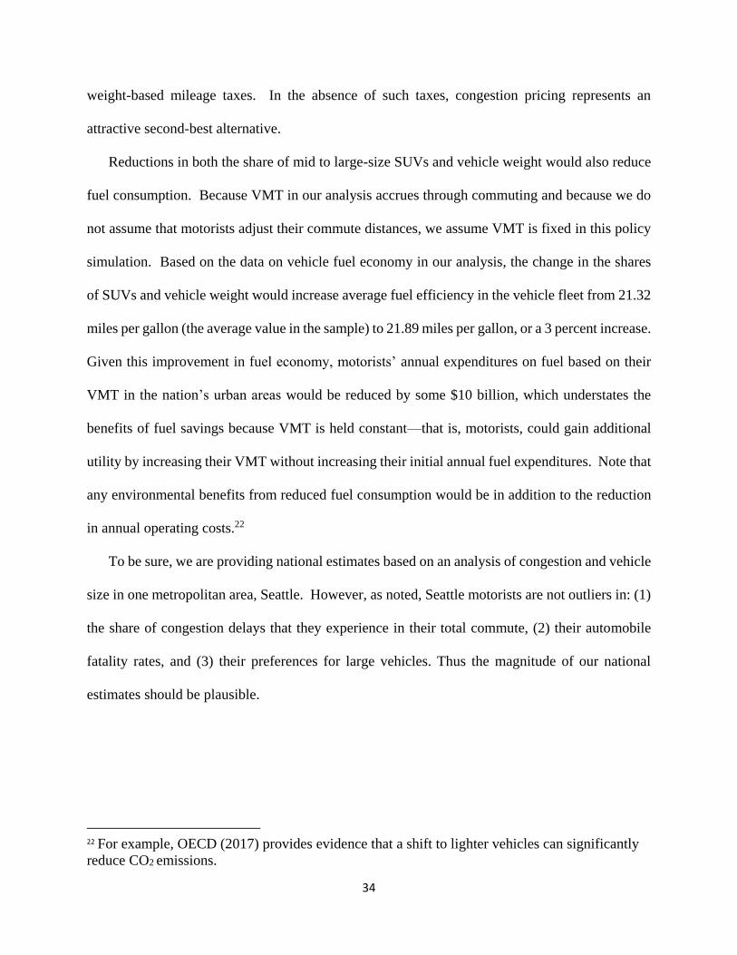
Reductions in both the share of mid to large-size SUVs and vehicle weight would also reduce
fuel consumption. Because VMT in our analysis accrues through commuting and because we do
not assume that motorists adjust their commute distances, we assume VMT is fixed in this policy
simulation. Based on the data on vehicle fuel economy in our analysis, the change in the shares
of SUVs and vehicle weight would increase average fuel efficiency in the vehicle fleet from 21.32
miles per gallon (the average value in the sample) to 21.89 miles per gallon, or a 3 percent increase.
Given this improvement in fuel economy, motorists’ annual expenditures on fuel based on their
VMT in the nation’s urban areas would be reduced by some $10 billion, which understates the
benefits of fuel savings because VMT is held constant—that is, motorists, could gain additional
utility by increasing their VMT without increasing their initial annual fuel expenditures. Note that
any environmental benefits from reduced fuel consumption would be in addition to the reduction
in annual operating costs.22
To be sure, we are providing national estimates based on an analysis of congestion and vehicle
size in one metropolitan area, Seattle. However, as noted, Seattle motorists are not outliers in: (1)
the share of congestion delays that they experience in their total commute, (2) their automobile
fatality rates, and (3) their preferences for large vehicles. Thus the magnitude of our national
estimates should be plausible.
22 For example, OECD (2017) provides evidence that a shift to lighter vehicles can significantly
reduce CO2 emissions.

35
7. Final Comments
Technological change has spurred an “arms race” on American roads, leading to larger and
more powerful vehicles that increase the negative safety and fuel consumption externalities from
automobile travel. Consumers’ preference for larger vehicles over smaller vehicles has persisted
despite the recent slowdown in total vehicle sales and the decline in real gasoline prices has
strengthened that preference. Further technological advance suggests that the arms race is likely
to continue for the foreseeable future. For example, SUVs are likely to improve their fuel economy
because of new technology that would enable their engines to shut down and restart when the
vehicle is idling. In addition, Mazda and Nissan, among other automakers, have made investments
that have resulted in efficiency improvements in internal combustion engine technologies.
Although electric vehicles are likely to eventually replace the internal combustion engine, their
expensive batteries and limited range and temperature driven performance constraints suggest that
considerable uncertainty exists as to when they will be able to do so.
We have analyzed highway congestion’s effect on the arms race by developing a dynamic
model of vehicle size choice and replacement and by analyzing how congestion pricing, which is
the efficient approach for addressing highway congestion externalities, could also address the
complementary negative externalities—reduced safety and greater fuel consumption—that arise
because of congestion’s positive effect on vehicle size. In the process, we have taken a plausible
approach to control for the endogenous choice of residential location and the omitted influences
that may affect both vehicle size and location decisions and potentially bias our parameter
estimates. Endogenous location decisions are also relevant for several other transportation
decisions, such as scheduling work trips (Small (1982)); we suggest future research should account
for those decisions to avoid potential bias.
36
Previous research has documented that congestion pricing can reduce the congestion
externality (Lindsey (2012)). Our findings extend that research by indicating that congestion
pricing could: (1) simultaneously decrease all of the major automobile externalities by reducing
vehicle sizes and congestion, (2) generate additional social benefits that have not been estimated
previously, and (3) become more politically attractive because, in contrast to conventional
criticisms that congestion pricing primarily benefits affluent motorists with a high value of travel
time, its benefits would be widely shared among all motorists and the public.
Importantly, our findings add support to VMT taxes that are currently being tested and under
serious consideration by several states on the west and east coasts because it would not be difficult
to allow those taxes to vary on different roads in accordance with traffic volumes (Langer,
Maheshri, and Winston (2017)). Looking to the future, implementing such taxes has taken on
additional importance because societies are preparing for the adoption of autonomous vehicles,
which are expected to reduce fatalities dramatically. But their effect on congestion and the
environment is less clear because of uncertainties over whether they will spur additional driving;
thus, an externality-based VMT tax would be socially desirable while contributing to more socially
optimal vehicle sizes.

37
References
Altonji, Joseph G., Todd E. Elder, and Christopher R. Taber. 2005. “Selection on Observed and
Unobserved Variables: Assessing the Effectiveness of Catholic Schools,” Journal of
Political Economy, volume 113, February, pp. 151-184.
Anderson, Michael L. and Max Auffhammer. 2014. “Pounds that Kill: The External Costs of
Vehicle Weight,” Review of Economic Studies, volume 81, April, pp. 535-571.
Anderson, Soren T., Ryan Kellogg, and James M. Sallee. 2013. “What Do Consumers Believe
About Future Gasoline Prices?,” Journal of Environmental Economics and Management,
volume 66, November, pp. 383-403.
Berry, Steven, James Levinsohn, and Ariel Pakes. 1995. “Automobile Prices in Market
Equilibrium,” Econometrica, volume 63, July, pp. 841-890.
Bradsher, Keith. 2002. High and Mighty: SUVs—The World’s Most Dangerous Vehicles And
How They Got That Way, PublicAffairs, New York.
Brownstone, David and Hao Fang. 2014. “A Vehicle Ownership and Utilization Choice Model
with Endogenous Residential Density,” Journal of Transport and Land Use, volume 7,
Number 2, pp. 135-151.
Brownstone, David and Thomas F. Golob. 2009. “The Impact of Residential Density on Vehicle
Usage and Energy Consumption,” Journal of Urban Economics, volume 65, January,
pp. 91-98.
Calfee, John and Clifford Winston. 1998. “The Value of Automobile Travel Time: Implications
for Congestion Policy,” Journal of Public Economics, volume 69, July, pp. 83-102.
Gladwell, Malcolm. 2004. “Big and Bad: How the SUV Ran Over Automobile Safety,” New
Yorker, January 12.
Gowrisankran, Gautam and Marc Rysman. 2012. “Dynamics of Consumer Demand for New
Durable Goods,” Journal of Political Economy, volume 120, December, pp. 1173-1219.
Green, Colin P., John S. Heywood, and Maria Navarro. 2016. “Traffic Accidents and the London
Congestion Charge,” Journal of Public Economics, volume 133, January, pp. 11-22.
Jacobsen, Mark R. 2013. “Fuel Economy and Safety: The Influences of Vehicle Class and Driver
Behavior,” American Economic Journal: Applied Economics, volume 5, July, pp. 1-26.
Khoeini, Sara and Randall Guensler. 2013. “Analysis of Fleet Composition and Vehicle Value
for the Atlanta I-85 HOT Lane,” presented at the 92nd Annual Meeting of the Transportation
Research Board, Washington, D.C.
38
Knittel, Christopher R. 2011. “Automobiles on Steroids: Product Attribute Trade-Offs and
Technological Progress in the Automobile Sector,” American Economic Review, volume
101, December, pp. 3368-3399.
Lancaster, Tony. 2000. “The Incidental Parameter Problem Since 1948,” Journal of
Econometrics, volume 95, April, pp. 391-413.
Langer, Ashley, Vikram Maheshri, and Clifford Winston. 2017. “From Gallons to Miles: A
Disaggregate Analysis of Automobile Travel and Externality Taxes,” Journal of Public
Economics, volume 152, August, pp. 34-46.
Li, Shanjun. 2012. “Traffic Safety and Vehicle Choice: Quantifying the Effects of the ‘Arms
Race’on American Roads,” Journal of Applied Econometrics, volume 27, January/February,
pp. 34-62.
Lindsey, Robin. 2012. “Road Pricing and Investment,” Economics of Transportation, volume
1, December, pp. 49-63.
Makuch, Kim. 2015. “The External Congestion Costs of Light Trucks,” unpublished University
of California, Irvine working paper.
Mannering, Fred and Clifford Winston. 1985. “A Dynamic Empirical Analysis of Household
Vehicle Ownership and Utilization,” Rand Journal of Economics, volume 16, Summer,
pp. 215-236.
Mannering, Fred, Clifford Winston, and William Starkey. 2002. “An Exploratory Analysis of
Automobile Leasing by US Households,” Journal of Urban Economics, volume 52, July,
pp. 154-176.
Manski, Charles F. and Steven R. Lerman. 1977. “The Estimation of Choice Probabilities from
Choice Based Samples,” Econometrica, volume 45, November, pp. 1977-1988.
McFadden, Daniel. 1981. “Econometric Models of Probabilistic Choice,” in C. Manski and
D. McFadden, editors, Structural Analysis of Discrete Data with Econometric Applications,
MIT Press, Cambridge, Massachusetts, pp. 198-272.
McFadden, Daniel. 1978. “Modelling the Choice of Residential Location,” in A. Karlqvist et al.,
editors, Spatial Interaction Theory and Residential Location, North Holland, Amsterdam,
pp. 75-96.
OECD. 2017. Lightening Up: How Less Heavy Vehicles Can Help Cut CO2 Emissions,
International Transport Forum, Paris, France.
Ossiander, Eric M., Thomas D. Koepsell, and Barbara McKnight. 2014. “Crash Fatality Risk and
Unibody Versus Body-On-Frame Structure in SUVs,” Accident Analysis and Prevention,
volume 70, September, pp. 267-272.

39
Rust, John. 1994. “Structural Estimation of Markov Decision Processes,” in James J. Heckman
and Edward E. Leamer, editors, Handbook of Econometrics, Volume 4, North Holland,
Elsevier Press, Amsterdam, pp. 3081-3143.
Schiraldi, Pasquale. 2011. “Automobile Replacement: A Dynamic Structural Approach,” RAND
Journal of Economics, volume 42, Summer, pp. 266-291.
Small, Kenneth A. 1982. “The Scheduling of Consumer Activities: Work Trips,” American
Economic Review, volume 72, June, pp. 467-479.
Small, Kenneth A., Clifford Winston, and Jia Yan. 2006. “Differentiated Road Pricing, Express
Lanes, and Carpools: Exploiting Heterogeneous Preferences in Policy Design,” Brookings-
Wharton Papers on Urban Affairs, pp. 53-96.
Train, Kenneth E. 2003. Discrete Choice Models with Simulation, Cambridge University Press,
Cambridge, United Kingdom.
Train, Kenneth and Clifford Winston. 2007. “Vehicle Choice Behavior and the Declining Market
Share of U.S. Automakers,” International Economic Review, volume 48, November, pp.
1469-1496.
White, Michelle J. 2004. “The ‘Arms Race’ on American Roads: The Effect of Sport Utility
Vehicles and Pickup Trucks on Traffic Safety,” Journal of Law and Economics, volume 47,
October, pp. 333-355.
Winston, Clifford. 2013. “On the Performance of the U.S. Transportation System: Caution
Ahead,” Journal of Economic Literature, volume 51, September, pp. 773-824.
Yeo, Hwasoo, Kitae Jang, and Alexander Skabardonis. 2010. “Impact of Traffic States on
Freeway Collision Frequency,” http://escholarship.org/uc/item/1v9383k9
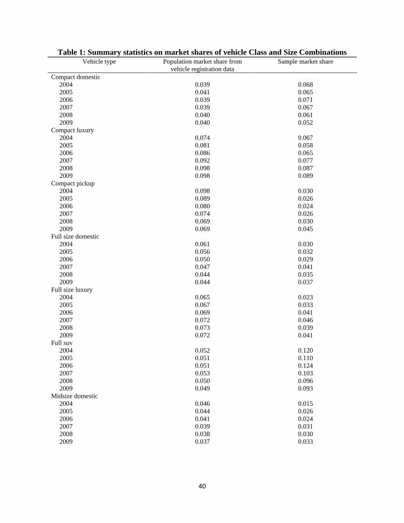
40
Table 1: Summary statistics on market shares of vehicle Class and Size Combinations Vehicle type Population market share from
vehicle registration data
Sample market share
Compact domestic
2004
2005
2006
2007
2008
2009
0.039
0.041
0.039
0.039
0.040
0.040
0.068
0.065
0.071
0.067
0.061
0.052
Compact luxury
2004
2005
2006
2007
2008
2009
0.074
0.081
0.086
0.092
0.098
0.098
0.067
0.058
0.065
0.077
0.087
0.089
Compact pickup
2004
2005
2006
2007
2008
2009
0.098
0.089
0.080
0.074
0.069
0.069
0.030
0.026
0.024
0.026
0.030
0.045
Full size domestic
2004
2005
2006
2007
2008
2009
0.061
0.056
0.050
0.047
0.044
0.044
0.030
0.032
0.029
0.041
0.035
0.037
Full size luxury
2004
2005
2006
2007
2008
2009
0.065
0.067
0.069
0.072
0.073
0.072
0.023
0.033
0.041
0.046
0.039
0.041
Full suv
2004
2005
2006
2007
2008
2009
0.052
0.051
0.051
0.053
0.050
0.049
0.120
0.110
0.124
0.103
0.096
0.093
Midsize domestic
2004
2005
2006
2007
2008
2009
0.046
0.044
0.041
0.039
0.038
0.037
0.015
0.026
0.024
0.031
0.030
0.033

41
Table 1 continued: Summary statistics on market shares of vehicle Class and Size
Combinations
Midsize luxury
2004
2005
2006
2007
2008
2009
0.138
0.144
0.155
0.160
0.165
0.165
0.241
0.240
0.229
0.217
0.222
0.219
Midsize suv
2004
2005
2006
2007
2008
2009
0.160
0.163
0.168
0.167
0.170
0.170
0.196
0.195
0.188
0.201
0.200
0.175
Passenger van
2004
2005
2006
2007
2008
2009
0.089
0.086
0.082
0.078
0.076
0.077
0.068
0.065
0.065
0.077
0.074
0.074
Standard pickup
2004
2005
2006
2007
2008
2009
0.088
0.091
0.095
0.097
0.095
0.095
0.061
0.052
0.047
0.041
0.048
0.048
Subcompact domestic
2004
2005
2006
2007
2008
2009
0.022
0.020
0.019
0.020
0.021
0.021
0.023
0.019
0.023
0.015
0.013
0.019
Subcompact luxury
2004
2005
2006
2007
2008
2009
0.034
0.034
0.035
0.035
0.037
0.036
0.060
0.078
0.071
0.057
0.065
0.074

42
Table 2 Summary Statistics of Motorists’ Socio-demographic Variables
Variables Means1
Annual household income (dollars) 108,108 (48,779)
Household size 3.03 (1.38)
House square footage (000’s) 1.89 (0.78)
Zillow home price index at the zip code level 2.89 (1.05)
Annual median city household income (dollars) 50,515 (11,554)
People crime index at the zip code level 3.02 (1.49)
Property crime index at the zip code level 3.62 (1.40)
School index at the zip code level 0.64 (0.22)
Percentage of motorists with long commute time (greater than 1 hour) 65%
Number of motorists 230
Number of observations 866 1Standard deviations in parentheses.
Table 3 Summary Statistics of Vehicle Attributes
Variables Means1
Manufacturer’s Suggested Retail Price (dollars) 35,552 (18,157)
Miles per gallon 21.32 (3.87)
Horse power 229 (54)
Body weight in pounds (pounds) 3,860 (849) 1Standard deviations in parentheses.

43
Table 4 Baseline Results 1
Variables Myopic
choice
Dynamic
choice
Price (100 thousands) /Household Income per Capita (100 thousands) -0.9472
(0.1031)
-0.7220
(0.1121)
Operating Cost (gas price ($) per gallon/mpg) /Household Income per Capita -0.0383
(0.0105)
-0.0601
(0.0215)
Horse Power 0.9802
(0.4873)
1.0630
(0.7916)
Horse power/Body Weight -1.1826
(0.2349)
-1.1484
(0.4429)
New Vehicle 0.6115
(0.1222)
0.4925
(0.1111)
Vehicle more than 5 years old -0.6163
(0.1130)
-0.6209
(0.1735)
Household Size × Passenger Van 0.7846
(0.1103)
1.1545
(0.3523)
Household Income per Capita × Luxury vehicle 0.6543
(0.3405)
0.7844
(0.3661)
Delay × Full or mid-size SUV 0.6875
(0.1988)
0.8182
(0.3012)
Delay × Body Weight 3.5638
(1.7290)
4.9771
(2.6111)
Delay × (Operating cost / Household income per capita) -0.1915
(0.0471)
-0.3633
(0.0691)
Std. Dev. of large vehicle dummy 2 0.1884
(0.1787)
0.1141
(0.1553)
Std. Dev. of luxury vehicle dummy 3 0.3618
(0.2448)
0.3166
(0.3288)
Std. Dev. of SUV dummy 0.2640
(0.1312)
0.3865
(0.1774)
Std. Dev. of new vehicle dummy 0.5444
(0.2630)
0.7231
(0.3340)
Alternative constants included YES YES
Interactions between Full or mid-size SUV/body weight / operating cost per
capita and demographic variables included 4
YES
YES
Interactions between Full or mid-size SUV/body weight/ operating cost per
capita and housing/residential location characteristics included 5
YES
YES
Log-likelihood value -3770.79 -3758.21
Number of commuters 230 230
Number of observations 866 866
Notes:
1. Vehicle holding in 2004 is treated as the initial condition in estimation.
2. Large vehicles include medium or full-size sedan, medium or full-size SUV, standard pickup and passenger van.
3. Luxury vehicles include imported luxury vehicles of all sizes. 4. Demographic variables include gender, young (age <= 35), household size and household income-per-capita.
5. Housing and residential location characteristics include house square footage, Zillow Home Value Index of the
zip code, median house income of the zip code, school index of the zip code, personal crime index of the zip code
and property crime index of the zip code.
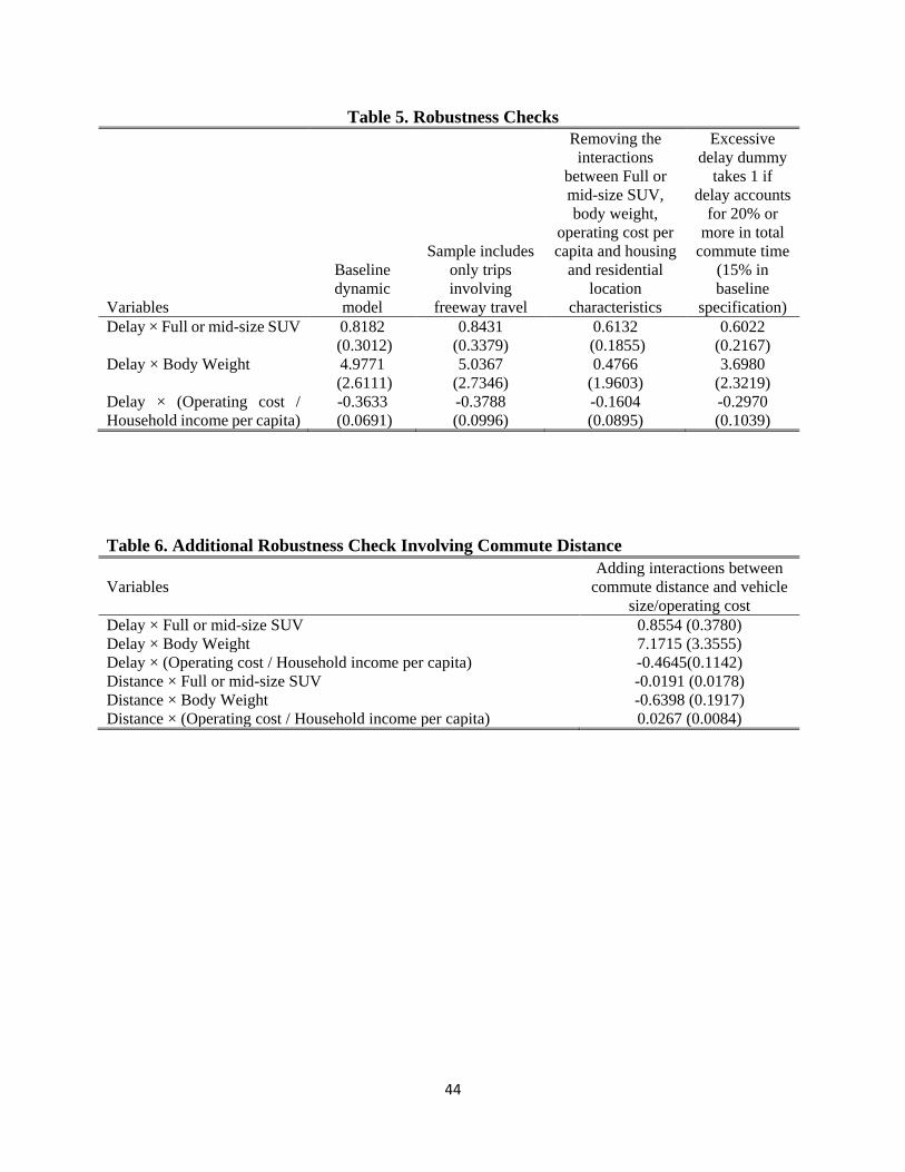
44
Table 5. Robustness Checks
Variables
Baseline
dynamic
model
Sample includes
only trips
involving
freeway travel
Removing the
interactions
between Full or
mid-size SUV,
body weight,
operating cost per
capita and housing
and residential
location
characteristics
Excessive
delay dummy
takes 1 if
delay accounts
for 20% or
more in total
commute time
(15% in
baseline
specification)
Delay × Full or mid-size SUV 0.8182
(0.3012)
0.8431
(0.3379)
0.6132
(0.1855)
0.6022
(0.2167)
Delay × Body Weight 4.9771
(2.6111)
5.0367
(2.7346)
0.4766
(1.9603)
3.6980
(2.3219)
Delay × (Operating cost /
Household income per capita)
-0.3633
(0.0691)
-0.3788
(0.0996)
-0.1604
(0.0895)
-0.2970
(0.1039)
Table 6. Additional Robustness Check Involving Commute Distance
Variables
Adding interactions between
commute distance and vehicle
size/operating cost
Delay × Full or mid-size SUV 0.8554 (0.3780)
Delay × Body Weight 7.1715 (3.3555)
Delay × (Operating cost / Household income per capita) -0.4645(0.1142)
Distance × Full or mid-size SUV -0.0191 (0.0178)
Distance × Body Weight -0.6398 (0.1917)
Distance × (Operating cost / Household income per capita) 0.0267 (0.0084)
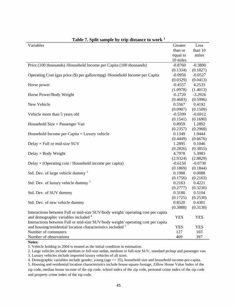
45
Table 7. Split sample by trip distance to work 1
Variables Greater
than or
equal to
10 miles
Less
than 10
miles
Price (100 thousands) /Household Income per Capita (100 thousands) -0.8760
(0.1334)
-0.3800
(0.1827)
Operating Cost (gas price ($) per gallon/mpg) /Household Income per Capita -0.0956
(0.0329)
-0.0527
(0.0413)
Horse power -0.4557
(1.0978)
4.2533
(1.4013)
Horse Power/Body Weight -0.2720
(0.4683)
-3.2926
(0.5996)
New Vehicle 0.5567
(0.0907)
0.4192
(0.1509)
Vehicle more than 5 years old -0.5599
(0.1541)
-0.6912
(0.1690)
Household Size × Passenger Van 0.8959
(0.2357)
1.2892
(0.2968)
Household Income per Capita × Luxury vehicle 0.1349
(0.4449)
1.9444
(0.6676)
Delay × Full or mid-size SUV 1.2895
(0.2826)
0.1046
(0.3855)
Delay × Body Weight 4.7978
(2.9324)
5.3983
(2.8829)
Delay × (Operating cost / Household income per capita) -0.6150
(0.1869)
-0.0730
(0.1844)
Std. Dev. of large vehicle dummy 2 0.1988
(0.1756)
0.0088
(0.2103)
Std. Dev. of luxury vehicle dummy 3 0.2163
(0.2777)
0.4221
(0.3230)
Std. Dev. of SUV dummy 0.3180
(0.1725)
0.5104
(0.2530)
Std. Dev. of new vehicle dummy 0.8520
(0.3888)
0.4301
(0.3130)
Interactions between Full or mid-size SUV/body weight/ operating cost per capita
and demographic variables included 4
YES
YES
Interactions between Full or mid-size SUV/body weight/ operating cost per capita
and housing/residential location characteristics included 5
YES
YES
Number of commuters 127 103
Number of observations 469 397
Notes:
1. Vehicle holding in 2004 is treated as the initial condition in estimation.
2. Large vehicles include medium or full-size sedan, medium or full-size SUV, standard pickup and passenger van.
3. Luxury vehicles include imported luxury vehicles of all sizes. 4. Demographic variables include gender, young (age <= 35), household size and household income-per-capita.
5. Housing and residential location characteristics include house square footage, Zillow Home Value Index of the
zip code, median house income of the zip code, school index of the zip code, personal crime index of the zip code
and property crime index of the zip code.
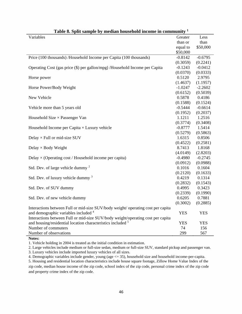
46
Table 8. Split sample by median household income in community 1
Variables Greater
than or
equal to
$50,000
Less
than
$50,000
Price (100 thousands) /Household Income per Capita (100 thousands) -0.8142
(0.3059)
-0.6795
(0.2241)
Operating Cost (gas price ($) per gallon/mpg) /Household Income per Capita -0.1243
(0.0370)
-0.0412
(0.0333)
Horse power 0.5120
(1.4637)
2.9795
(1.1957)
Horse Power/Body Weight -1.0247
(0.6152)
-2.2602
(0.5039)
New Vehicle 0.5878
(0.1588)
0.4186
(0.1524)
Vehicle more than 5 years old -0.5444
(0.1952)
-0.6614
(0.2037)
Household Size × Passenger Van 1.1211
(0.3774)
1.2516
(0.3408)
Household Income per Capita × Luxury vehicle -0.8777
(0.5279)
1.5414
(0.5863)
Delay × Full or mid-size SUV 1.6315
(0.4522)
0.8506
(0.2581)
Delay × Body Weight 8.7413
(4.0149)
1.8168
(2.8203)
Delay × (Operating cost / Household income per capita) -0.4980
(0.0912)
-0.2745
(0.0988)
Std. Dev. of large vehicle dummy 2 0.1016
(0.2120)
0.1604
(0.1633)
Std. Dev. of luxury vehicle dummy 3 0.4219
(0.2832)
0.1314
(0.1543)
Std. Dev. of SUV dummy 0.4995
(0.2339)
0.3423
(0.1990)
Std. Dev. of new vehicle dummy 0.6205
(0.3002)
0.7881
(0.2885)
Interactions between Full or mid-size SUV/body weight/ operating cost per capita
and demographic variables included 4
YES
YES
Interactions between Full or mid-size SUV/body weight/operating cost per capita
and housing/residential location characteristics included 5
YES
YES
Number of commuters 74 156
Number of observations 299 567
Notes:
1. Vehicle holding in 2004 is treated as the initial condition in estimation.
2. Large vehicles include medium or full-size sedan, medium or full-size SUV, standard pickup and passenger van.
3. Luxury vehicles include imported luxury vehicles of all sizes. 4. Demographic variables include gender, young (age <= 35), household size and household income-per-capita.
5. Housing and residential location characteristics include house square footage, Zillow Home Value Index of the
zip code, median house income of the zip code, school index of the zip code, personal crime index of the zip code
and property crime index of the zip code.
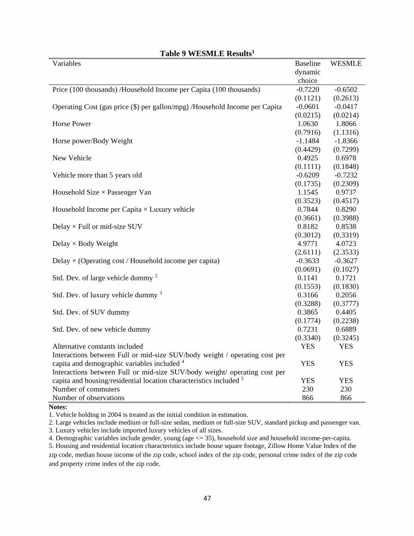
47
Table 9 WESMLE Results1
Variables Baseline
dynamic
choice
WESMLE
Price (100 thousands) /Household Income per Capita (100 thousands) -0.7220
(0.1121)
-0.6502
(0.2613)
Operating Cost (gas price ($) per gallon/mpg) /Household Income per Capita -0.0601
(0.0215)
-0.0417
(0.0214)
Horse Power 1.0630
(0.7916)
1.8066
(1.1316)
Horse power/Body Weight -1.1484
(0.4429)
-1.8366
(0.7299)
New Vehicle 0.4925
(0.1111)
0.6978
(0.1848)
Vehicle more than 5 years old -0.6209
(0.1735)
-0.7232
(0.2309)
Household Size × Passenger Van 1.1545
(0.3523)
0.9737
(0.4517)
Household Income per Capita × Luxury vehicle 0.7844
(0.3661)
0.8290
(0.3988)
Delay × Full or mid-size SUV 0.8182
(0.3012)
0.8538
(0.3319)
Delay × Body Weight 4.9771
(2.6111)
4.0723
(2.3533)
Delay × (Operating cost / Household income per capita) -0.3633
(0.0691)
-0.3627
(0.1027)
Std. Dev. of large vehicle dummy 2 0.1141
(0.1553)
0.1721
(0.1830)
Std. Dev. of luxury vehicle dummy 3 0.3166
(0.3288)
0.2056
(0.3777)
Std. Dev. of SUV dummy 0.3865
(0.1774)
0.4405
(0.2238)
Std. Dev. of new vehicle dummy 0.7231
(0.3340)
0.6889
(0.3245)
Alternative constants included YES YES
Interactions between Full or mid-size SUV/body weight / operating cost per
capita and demographic variables included 4
YES
YES
Interactions between Full or mid-size SUV/body weight/ operating cost per
capita and housing/residential location characteristics included 5
YES
YES
Number of commuters 230 230
Number of observations 866 866
Notes:
1. Vehicle holding in 2004 is treated as the initial condition in estimation.
2. Large vehicles include medium or full-size sedan, medium or full-size SUV, standard pickup and passenger van.
3. Luxury vehicles include imported luxury vehicles of all sizes. 4. Demographic variables include gender, young (age <= 35), household size and household income-per-capita.
5. Housing and residential location characteristics include house square footage, Zillow Home Value Index of the
zip code, median house income of the zip code, school index of the zip code, personal crime index of the zip code
and property crime index of the zip code.
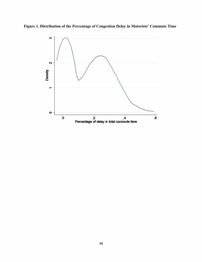
48
Figure 1. Distribution of the Percentage of Congestion Delay in Motorists’ Commute Time
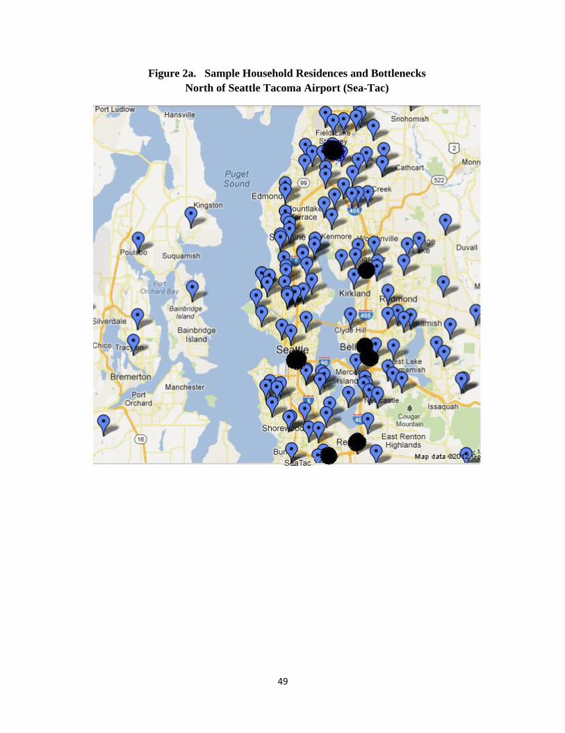
49
Figure 2a. Sample Household Residences and Bottlenecks
North of Seattle Tacoma Airport (Sea-Tac)
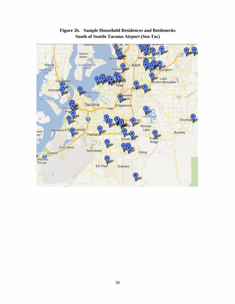
50
Figure 2b. Sample Household Residences and Bottlenecks
South of Seattle Tacoma Airport (Sea-Tac)

51
Figure 3. A Dynamic Model of a Decisionmaker’s Vehicle Holding and Replacement
Decisions
Figure 2: A dynamic model of an individual’s vehicle holding
t t+1
Owns a vehicle Has complete information
on the vehicle that is owned and on the vehicles available in the market
Preference shocks are realized
Receives information on the price of gasoline and formulates expectations of future gasoline prices
Decisionmaking: Hold the current vehicle
or replace it with another one
Stage 1 Stage 2 Stage 3
Utility realized
from driving the
vehicle


![arXiv:1706.07467v2 [stat.AP] 21 Nov 2019 · 2019-11-22 · socio-economical spatial process. ... negative externalities associated with the use of automobile (pollution, accidents,](https://img.pdfslide.us/doc/110x75/5f2fcfce47b3de03d16af255/arxiv170607467v2-statap-21-nov-2019-2019-11-22-socio-economical-spatial-process.jpg)