Embed Size (px)
Citation preview

Network Externalities and Market Dominance∗
Robert Akerlof† Richard Holden‡ Luis Rayo§
November 16, 2017
Abstract
We develop a simple framework in the spirit of Katz and Shapiro (1985)
and Becker (1991) to study pricing and competition in markets with network
externalities. We provide micro-foundations for a family of non-standard
“in/out” demand curves, with a positively-sloped intermediate region. We
also provide a simple theory of equilibrium selection that yields concise pre-
dictions regarding when firms will be “in” and when “out.” We use this
framework to provide a unified explanation for a variety of stylized facts
(some already accounted for, others not) including why: (i) it is difficult to
become “in”; (ii) the “in” position is fragile; (iii) “in” firms are not asleep in
the sense that they continuously raise quality and keep prices low; and (iv)
“in” firms acquire startups in order to entrench their position.
∗We are grateful to Gonzalo Cisternas, Luis Garicano, Bob Gibbons, Tom Hubbard, BobPindyck, and seminar participants at Kellogg, MIT, Melbourne, and UNSW for helpful discus-sions. Akerlof acknowledges support from the Institute for New Economic Thinking (INET).Holden acknowledges support from the Australian Research Council (ARC) Future FellowshipFT130101159. Rayo acknowledges support from the Marriner S. Eccles Institute for Economicsand Quantitative Analysis.†University of Warwick and CEPR, [email protected].‡UNSW Australia Business School, [email protected].§University of Utah and CEPR, [email protected].

1 Introduction
Recent decades have witnessed the rise of “superstar firms” that manage to take
over most of their markets (e.g. Autor et al. (2017)). Frequently, these firms pro-
duce goods that are both scalable (such as non-rival goods) and subject to network
effects whereby consumer demand is directly affected by peer consumption. For
example, Facebook, Microsoft, Google, and Uber all produce goods with essentially
zero marginal costs and whose consumers are arguably influenced by the overall
popularity of the product in question.1
Commonly, markets with scalable goods and network effects exhibit a series
of interrelated patterns:
First, winners serve a disproportionate share of their market, with a large size
gap between them and their closest rivals.
Secondly, it is difficult to become a winner and yet success is so fragile that
it can vanish overnight. The difficulties of becoming popular (going from being
“out” to being “in”) are illustrated by Microsoft’s search engine Bing, which de-
spite years of sizeable investments remains much smaller than the current super-
star Google. And the ease with which a successful firm can suddenly fail (going
from “in” to “out”) is illustrated by the web browser Netscape, which despite its
initial dominant status was overtaken quite suddenly by Microsoft’s Internet Ex-
plorer.
Finally, despite their seemingly dominant position, winners are not asleep.
This can be seen by the fact that winners tend to continuously raise quality (for
example, by purchasing new startups) while at the same time keeping their prices
low, sometimes even below average cost.
Our goal is to develop a tractable framework in the spirit of Katz and Shapiro
(1985) and Becker (1991) that provides a unified account for these patterns. In
addition, we use this framework to characterize the role and economic value of1 In 2002, Bill Gates summarized his ambitions as follows: “We look for opportunities with
network externalities — where there are advantages to the vast majority of consumers to sharea common standard. We look for businesses where we can garner large market shares, not just30-35%” (Rivkin and Van den Steen (2009)).
1

“influencers” (consumers capable of affecting a sizeable fraction of the popula-
tion), to discuss investment and firm acquisition decisions, and to argue that when
network externalities are strong, antitrust considerations differ significantly from
conventional approaches.
Katz and Shapiro (1985) and Becker (1991) first studied the role of network
externalities in models where peer consumption enters as a direct argument of a
consumer’s demand (in addition to price). They argue that network externalities
can generate demand curves with both downward- and upward-sloping regions,
depending on when the traditional price effect or the network effect dominates.
Such demand curves admit the possibility of multiple equilibria in terms of firm
size, and therefore the possibility of large industry winners.
What is somewhat less satisfying is these models is their treatment of equilib-
rium selection, which is for the most part absent, and their justification for a par-
ticular shape for the demand curve. In Katz and Shapiro’s model, the population
of consumers is assumed to be uniform; as a result, only through non-linearities
in the network externality can one obtain a non-standard demand curve. And in
Becker’s model, a non-standard demand with desirable properties is simply as-
sumed. In addition, while Becker argues persuasively that price is a somewhat
blunt instrument in affecting a move from the “small” equilibrium to the “large”
equilibrium, his argument in the other direction is less convincing.
Our model is closest to Becker’s, but with one ingredient left out, and one
added in. We dispense with his capacity constraint (i.e. goods in our model are
non-rivalrous), and we model the equilibrium selection or transition process ex-
plicitly. In addition, we provide a micro-foundation for a Becker-style demand
curve with alternating downward and upward sloping regions, which we call an
“in/out” demand curve. This micro-foundation shows that such non-standard
shape is quite easy to obtain, even when network externalities are linear, and in
fact should be expected to arise frequently in practice.
In our setting consumers may coordinate on a high or low level of demand.
This is somewhat analogous to a setting studied in Akerlof and Holden (2017) in
which investors can coordinate on a high or low level of investment in a project.
2
As in Akerlof and Holden (2017) we view the coordinating process as part of the
equilibrium and we consider how a firm might be able to coordinate consumers
on a high, rather than a low, level of demand.
The remainder of the paper is organized as follows. Section 3 presents the base-
line model with a single firm; Section 4 considers price competition among two
firms; Section 5 considers the special case of a piecewise linear “In/Out” demand
curve; and Section 6 concludes.
2 Monopoly Case
To begin, we will consider a setting with a single firm (a monopolist). We assume
that each period (t = 1, 2, ..., T ), the monopolist chooses a price pt. The marginal
cost of production is constant — and we normalize it to zero.
There is a set of consumers. Consumer i’s demand at time t, denoted qti ,
depends upon the price pt and upon aggregate consumption Qt; that is, qti =
Di(pt, Qt). We assume qti is decreasing in pt; and qti is increasing in Qt, reflecting
the presence of positive network externalities.
For any given pt, an equilibrium quantity Qt∗ satisfies:
Qt∗ =∑i
Di
(pt, Q
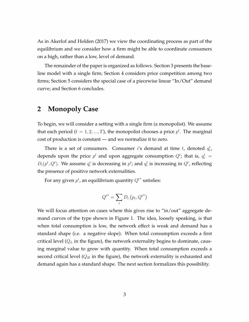
t∗)We will focus attention on cases where this gives rise to “in/out” aggregate de-
mand curves of the type shown in Figure 1. The idea, loosely speaking, is that
when total consumption is low, the network effect is weak and demand has a
standard shape (i.e. a negative slope). When total consumption exceeds a first
critical level (QL in the figure), the network externality begins to dominate, caus-
ing marginal value to grow with quantity. When total consumption exceeds a
second critical level (QH in the figure), the network externality is exhausted and
demand again has a standard shape. The next section formalizes this possibility.
3
“In/Out” Demand Curve“In/Out” Demand Curve
QH
QL
D
Q
pmax
pmin
p
Figure 1
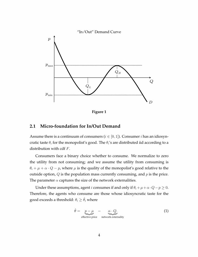
2.1 Micro-foundation for In/Out Demand
Assume there is a continuum of consumers (i ∈ [0, 1]). Consumer i has an idiosyn-
cratic taste θi for the monopolist’s good. The θi’s are distributed iid according to a
distribution with cdf F .
Consumers face a binary choice whether to consume. We normalize to zero
the utility from not consuming; and we assume the utility from consuming is
θi + µ + α · Q − p, where µ is the quality of the monopolist’s good relative to the
outside option, Q is the population mass currently consuming, and p is the price.
The parameter α captures the size of the network externalities.
Under these assumptions, agent i consumes if and only if θi+µ+α ·Q−p ≥ 0.
Therefore, the agents who consume are those whose idiosyncratic taste for the
good exceeds a threshold: θi ≥ θ̂, where
θ̂ = p− µ︸ ︷︷ ︸effective price
− α ·Q.︸ ︷︷ ︸network externality
(1)
4
The threshold is increasing in the good’s “effective price” (the price net of quality)
and it is decreasing in the size of the network externality.
Observe that aggregate demandQ is equal to the mass of consumers above the
threshold:
Q = 1− F (θ̂). (2)
Combining equations (1) and (2), we find that:
Q = 1− F (p− µ− α ·Q). (3)
Rearranging terms, we obtain a formula for (inverse) demand:
pd(Q) = F−1(1−Q) + α ·Q+ µ. (4)
Notice from equation (4) that µ, the good’s quality relative to the outside option,
shifts the demand curve vertically. An increase in the good’s quality shifts de-
mand vertically up while an increase in the outside option shifts demand verti-
cally down.
We can differentiate equation (4) to obtain an expression for the slope of de-
mand:dpd(Q)
dQ= α︸︷︷︸
network externality
− 1
f(F−1(1−Q)).︸ ︷︷ ︸
distribution of consumers’ tastes
(5)
The slope depends both upon the size of network externalities (term 1) and the
distribution of consumers’ tastes (term 2). Demand is downward-sloping in the
absence of network externalities; but demand may be positively sloped when net-
work externalities are present.
From here, it is easy to obtain an in/out demand curve. Suppose, for instance,
F is a normal distribution with mean 0 and variance σ2. The demand curve has
a maximum slope of α − 1f(0)
= α −√
2πσ2 (at Q = 12). The demand curve has
a minimum slope of α − 1f(±∞)
= −∞ (at Q = 0 and Q = 1). Demand has an
in/out shape, as in Figure 1, if the network externalities are sufficiently large (α >
5
(a) Demand curve solves: Q = 1− F (p− µ− αQ)
Q
Q (45̊ line)
1–F(p– μ –αQ)
Qmid(p)Qout(p) Qin(p)
Higher p
(b) “In/Out” Demand Curve
D
Q
pmax
pmin
p
Qout(p) Qmid(p) Qin(p)
p
Figure 2
6
√2πσ2).2
More generally, if F has support R and the pdf is single-peaked:
1. Demand is downward-sloping if α ≤ α̂.
2. Demand is “in/out” if α > α̂.
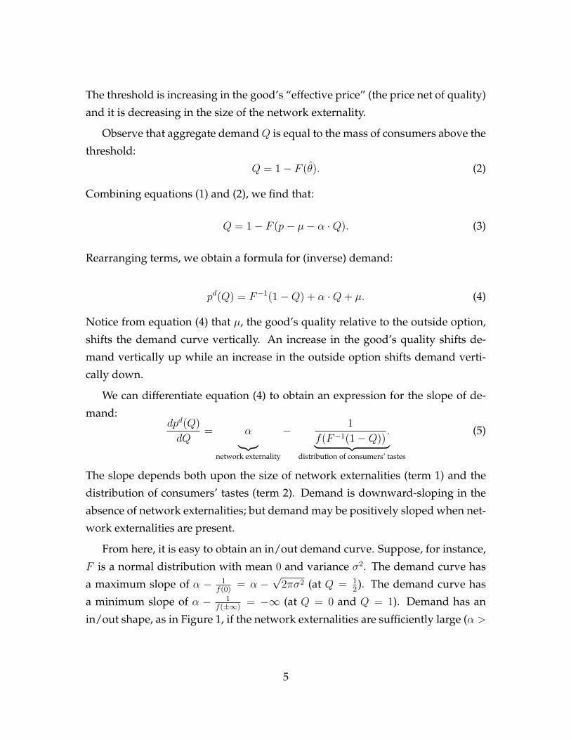
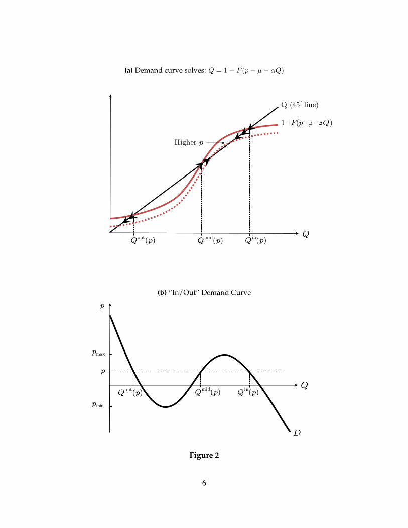
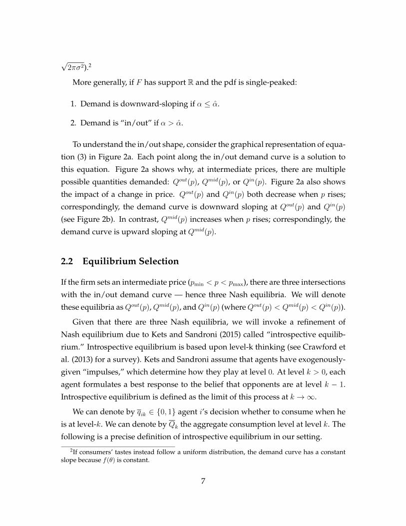
To understand the in/out shape, consider the graphical representation of equa-
tion (3) in Figure 2a. Each point along the in/out demand curve is a solution to
this equation. Figure 2a shows why, at intermediate prices, there are multiple
possible quantities demanded: Qout(p), Qmid(p), or Qin(p). Figure 2a also shows
the impact of a change in price. Qout(p) and Qin(p) both decrease when p rises;
correspondingly, the demand curve is downward sloping at Qout(p) and Qin(p)
(see Figure 2b). In contrast, Qmid(p) increases when p rises; correspondingly, the
demand curve is upward sloping at Qmid(p).
2.2 Equilibrium Selection
If the firm sets an intermediate price (pmin < p < pmax), there are three intersections
with the in/out demand curve — hence three Nash equilibria. We will denote
these equilibria asQout(p),Qmid(p), andQin(p) (whereQout(p) < Qmid(p) < Qin(p)).
Given that there are three Nash equilibria, we will invoke a refinement of
Nash equilibrium due to Kets and Sandroni (2015) called “introspective equilib-
rium.” Introspective equilibrium is based upon level-k thinking (see Crawford et
al. (2013) for a survey). Kets and Sandroni assume that agents have exogenously-
given “impulses,” which determine how they play at level 0. At level k > 0, each
agent formulates a best response to the belief that opponents are at level k − 1.
Introspective equilibrium is defined as the limit of this process at k →∞.
We can denote by qik ∈ {0, 1} agent i’s decision whether to consume when he
is at level-k. We can denote by Qk the aggregate consumption level at level k. The
following is a precise definition of introspective equilibrium in our setting.
2If consumers’ tastes instead follow a uniform distribution, the demand curve has a constantslope because f(θ) is constant.
7
Definition 1 (Introspective Equilibrium).
1. Fix p and take consumers’ level-0 choices, called “impulses,” as given: qi0. The
“aggregate impulse” is Q0.
2. Level k is obtained by assuming consumers best-respond to price p and the belief
that other consumers are at level k − 1: qik, Qk.
3. An introspective equilibrium is the limit as k →∞: q∗i , Q∗.
Introspective equilibrium is very general. It nests a wide range of refinement
concepts, corresponding to different assumptions about agents’ impulses. Risk
dominance, for instance, corresponds to the case where agents are uncertain about
each others’ impulses. We make what we think is a natural assumption in our
setting. We assume each agent’s impulse is to do what she did in the previous
period: qi0 = qt−1i . Therefore the aggregate impulse is Q0 = Qt−1. We take agents’
impulses in the first period as exogenous and denote them as q0i and Q0. Proposi-
tion 1 derives the introspective equilibrium as a function of the aggregate impulse
(Qt−1).
Proposition 1. The unique introspective equilibrium is:
Q∗(p,Qt−1
)=
Qin(p), if Qt−1 > Qmid(p).
Qmid(p), if Qt−1 = Qmid(p).
Qout(p), if Qt−1 < Qmid(p).
Proof of Proposition 1
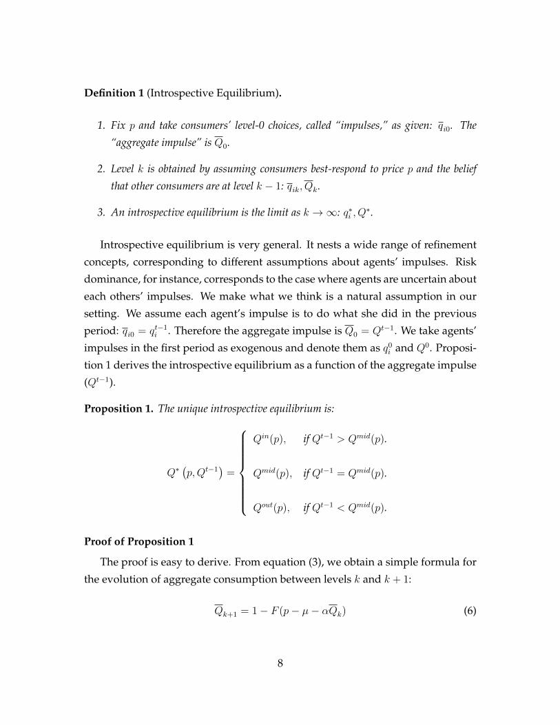
The proof is easy to derive. From equation (3), we obtain a simple formula for
the evolution of aggregate consumption between levels k and k + 1:
Qk+1 = 1− F (p− µ− αQk) (6)
8
Qk+1 = 1− F (p− µ− αQk)
Qk
Qk+1
1 – F(p – μ – α Qk)
Qt–1
Qk+1 = Qk
Qmid(p)Qout(p) Qin(p)Qt–1
Figure 3
Figure 3 corresponds to equation (6). It shows how, starting from an initial im-
pulse (Qt−1), the aggregate consumption level evolves.
Observe that, if there is a high initial impulse to consume (Qt−1 > Qmid(p)),
aggregate consumption increases between levels 0 and 1. Intuitively, the high level
of consumption at level 0 drives more agents to consume at level 1. Consumption
continues to increase between levels 2 and 3, 3 and 4, and so forth, reaching Qin(p)
in the limit. Hence, when Qt−1 > Qmid(p), the introspective equilibrium is Qin(p).
By a similar logic, aggregate consumption falls between successive levels when
Qt−1 < Qmid(p). When Qt−1 < Qmid(p), the introspective equilibrium is Qout(p).
Q.E.D.
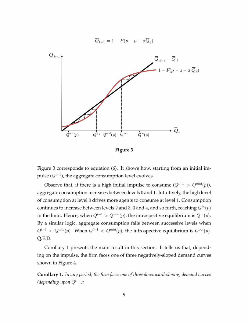
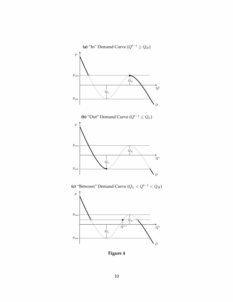
Corollary 1 presents the main result in this section. It tells us that, depend-
ing on the impulse, the firm faces one of three negatively-sloped demand curves
shown in Figure 4.
Corollary 1. In any period, the firm faces one of three downward-sloping demand curves
(depending upon Qt−1):
9
(a) “In” Demand Curve (Qt−1 ≥ QH )“In” Demand Curve (Q t–1 ≥ QH)
QH
QL
D
Q t
pmax
pmin
p
(b) “Out” Demand Curve (Qt−1 ≤ QL)“Out” Demand Curve (Q t–1 ≤ QL)
QH
QL
D
Q t
pmax
pmin
p
(c) “Between” Demand Curve (QL < Qt−1 < QH )“Between” Demand Curve: (QL < Q t–1 < QH)
QH
QL
D
Q t
pmax
pmin
p
Q t–1
Figure 4
10

1. “In” Demand Curve (Qt−1 ≥ QH).
2. “Out” Demand Curve (Qt−1 ≤ QL).
3. “Between” Demand Curve (QL < Qt−1 < QH).
If Qt−1 ≥ QH , the introspective equilibrium is always Qin(p). We will say that
the firm is “in” when Qt−1 ≥ QH . The firm, in this case, faces an “in” demand
curve (shown in Figure 4a).
If Qt−1 ≤ QL, the introspective equilibrium is always Qout(p). We will say that
the firm is “out” when Qt−1 ≤ QL. The firm, in this case, faces an “out” demand
curve (shown in Figure 4b).
If QL < Qt−1 < QH , we will say that the firm is “between.” The firm, in this
case, faces a “between” demand curve (shown in Figure 4c).
2.3 Optimal Pricing
We are now in a position to formally state the monopolist’s problem and describe
optimal pricing.
In each of the T periods, the monopolist chooses price to maximize the dis-
counted sum of future profits. The monopolist’s discount factor is δ. Period t
profits are πt = pt · Qt, and Qt = Q∗(pt, Qt−1) (where Q∗(pt, Qt−1) is defined as in
Proposition 1). We take Q0, the initial consumption level or impulse, as given.
First, suppose the firm is myopic (δ = 0), caring only about current profits.
There are three cases (see Lemma 1).
Lemma 1. Suppose the firm is myopic (δ = 0). Depending upon the shape of the demand
curve (which is a function of α, µ, and F ), there are three cases:
(i) It is optimal to go “in” in period t (choose pt such that Qt ≥ QH) regardless of the
value of Qt−1.
(ii) It is optimal to go “out” in period t (choose pt such that Qt ≤ QL) regardless of the
value of Qt−1.
11
(iii) It is optimal for “in” (“out”) firms to stay “in” (“out”). “Between” firms go “in”
(“out”) if Qt−1 is above (below) a cutoff (Qmyopic).
One implication of Lemma 1 is that firms that are initially “between” (QL <
Q0 < QH) never remain “between”: they either become “in” or “out.” The reason
is as follows. To remain between, the firm would need to choose a price p1 such
that Q1 = Q0. But, as Figure 4c shows, starting at such a price, a small decrease in
the price increases demand by a discontinuous amount. Thus, the hypothesized
price cannot be optimal.
Now, suppose the firm is not myopic (δ > 0). Proposition 2 compares the
optimal pricing with that of a myopic firm.
Proposition 2. Suppose the firm is not myopic. In cases (i) and (ii) in Lemma 1, the
firm acts as if it were myopic. In case (iii), “out” and “between” firms potentially act
non-myopically in period 1. Specifically, if Q0 exceeds a cutoff (Qnon-myopic < Qmyopic), the
firm prices below the myopic level in period 1; it goes “in” and stays “in” in subsequent
periods.
Intuitively, “out” and “between” firms have an incentive to price below the
myopic level in order to become “in” in subsequent periods. The benefit of being
“in” is that “in” firms face a better demand curve than “out” firms (see Figure 4).
In practice, some firms charge no money to their consumers. Notable exam-
ples are search engines (e.g. Google, Bing, Yahoo) and web browsers (e.g. Firefox,
Chrome, Safari, Internet Explorer). In these instances, firms profit by showing
advertisements to their users and/or by directing user traffic to other products.
Since, in the margin, these practices reduce consumer value, they can be inter-
preted as a positive price.
2.4 Influencers
Suppose an “influencer” is connected to a fraction φ of the consumers and has the
ability to shift those consumers’ impulses: from “don’t consume” to “consume”
or vice-versa. Let b ∈ {0, 1} denote the influencer’s choice whether to shift con-
sumers’ impulses to “consume” or “don’t consume.”
12
The influencer can play a pivotal role in determining whether the firm is “in”
or “out,” as the following corollary to Proposition 1 demonstrates.
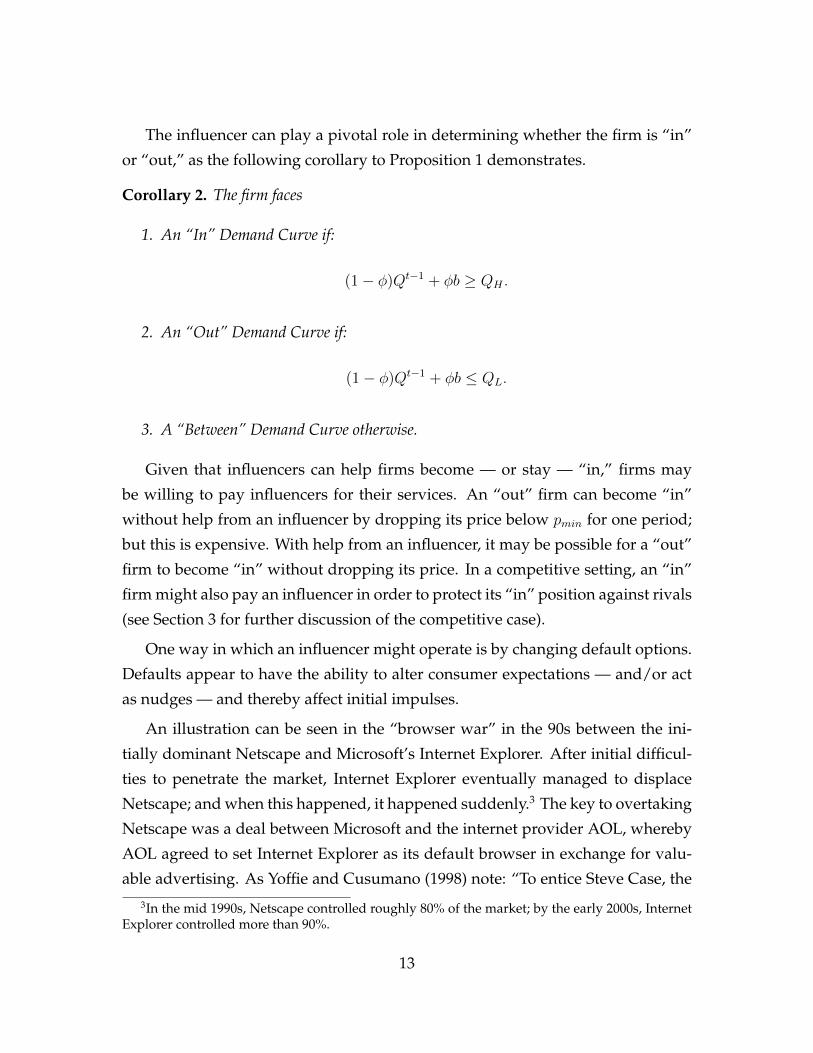
Corollary 2. The firm faces
1. An “In” Demand Curve if:
(1− φ)Qt−1 + φb ≥ QH .
2. An “Out” Demand Curve if:
(1− φ)Qt−1 + φb ≤ QL.
3. A “Between” Demand Curve otherwise.
Given that influencers can help firms become — or stay — “in,” firms may
be willing to pay influencers for their services. An “out” firm can become “in”
without help from an influencer by dropping its price below pmin for one period;
but this is expensive. With help from an influencer, it may be possible for a “out”
firm to become “in” without dropping its price. In a competitive setting, an “in”
firm might also pay an influencer in order to protect its “in” position against rivals
(see Section 3 for further discussion of the competitive case).
One way in which an influencer might operate is by changing default options.
Defaults appear to have the ability to alter consumer expectations — and/or act
as nudges — and thereby affect initial impulses.
An illustration can be seen in the “browser war” in the 90s between the ini-
tially dominant Netscape and Microsoft’s Internet Explorer. After initial difficul-
ties to penetrate the market, Internet Explorer eventually managed to displace
Netscape; and when this happened, it happened suddenly.3 The key to overtaking
Netscape was a deal between Microsoft and the internet provider AOL, whereby
AOL agreed to set Internet Explorer as its default browser in exchange for valu-
able advertising. As Yoffie and Cusumano (1998) note: “To entice Steve Case, the3In the mid 1990s, Netscape controlled roughly 80% of the market; by the early 2000s, Internet
Explorer controlled more than 90%.
13

CEO of AOL, to make Internet Explorer AOL’s preferred browser, Gates offered
to put an AOL icon on the Windows 95 desktop, perhaps the most expensive real
estate in the world. In exchange for promoting Internet Explorer as its default
browser, AOL would have almost equal importance with [AOL’s rival] MSN on
future versions of Windows.” To this day, the browser wars continue, with smart-
phones being the latest battlefront. Here again, defaults appear to play a major
role (e.g. Cain Miller (2012)).
Remark: Large Consumers
Suppose, in addition to small consumers, there is a large consumer who, when
he purchases the monopolist’s good, purchases a large quantity. Like an influ-
encer, a large consumer can help tip the monopolist from “out” to “in.” Conse-
quently, one would expect the monopolist to pay the large consumer a rent —
just as he would pay a rent to an influencer. This rent might take the form of a
discount relative to the price charged to small consumers.
3 Competition
It is a simple step to move from a monopoly setting to a competitive setting. Sup-
pose there are two firms (1 and 2) that engage in price competition. At stage 1,
firm 1 sets price p1. At stage 2, firm 2 sets price p2.
We continue to assume there is a continuum of consumers (i ∈ [0, 1]) with
tastes θi distributed F . Now, θi represents consumer i’s taste for good 1 relative to
good 2. Consumers make a binary choice whether to consume good 1 or good 2.
Hence, overall demand sums to 1: Q1 +Q2 = 1. The utility from consuming good
1 is θi + µ + α · Q1 − p1, where µ denotes the quality of good 1 relative to good 2.
The utility from consuming good 2 is α ·Q2 − p2.
Under these assumptions, demand for each good depends upon the price dif-
ferential: ∆ = p1 − p2. We will focus on cases where this gives rise to in/out
demand, as pictured in Figure 5. Observe that, whenever demand for good 1 is
14
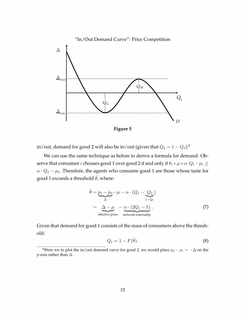
“In/Out Demand Curve”: Price Competition“In/Out” Demand Curve: Bertrand Competition
QH
QL
D
max
min
Q
1
Figure 5
in/out, demand for good 2 will also be in/out (given that Q2 = 1−Q1).4
We can use the same technique as before to derive a formula for demand. Ob-
serve that consumer i chooses good 1 over good 2 if and only if θi+µ+α·Q1−p1 ≥α · Q2 − p2. Therefore, the agents who consume good 1 are those whose taste for
good 1 exceeds a threshold θ̂, where:
θ̂ = p1 − p2︸ ︷︷ ︸∆
−µ− α · (Q1 − Q2︸︷︷︸1−Q1
)
= ∆− µ︸ ︷︷ ︸effective price
− α · (2Q1 − 1)︸ ︷︷ ︸network externality
. (7)
Given that demand for good 1 consists of the mass of consumers above the thresh-
old:
Q1 = 1− F (θ̂). (8)
4Were we to plot the in/out demand curve for good 2, we would place p2 − p1 = −∆ on they-axis rather than ∆.
15
Combining (7) and (8), we obtain an analog of equation (3):
Q1 = 1− F (∆− µ− α · (2Q1 − 1)). (9)
Rearranging terms yields an expression for the (inverse) demand for good 1:
∆d(Q1) = µ+ α · (2Q1 − 1) + F−1(1−Q1). (10)
Observe that a change in the quality of good 1 relative to good 2, µ, shifts de-
mand vertically. Differentiating equation (10), we obtain a formula for the slope
of demand:
d∆d(Q)1
dQ1
= 2α︸︷︷︸network externality
− 1
f(F−1(1−Q1)).︸ ︷︷ ︸
distribution of consumers’ tastes
(11)
As before, if F has support R and the pdf is single-peaked:
1. Demand is downward-sloping if α ≤ α̂.
2. Demand is “in/out” if α > α̂.
Remark: Product Compatibility
The existing literature on network externalities has highlighted product com-
patibility as an issue of interest: particularly, the incentives of firms to make their
products compatible (see, for instance, Katz and Shapiro (1994)).
It is easy to incorporate into our framework the idea that competing products
may be more or less compatible. Suppose the utility from consuming good 1 is
θi+µ+α·(Q1+γQ2)−p1 and the utility from consuming good 2 is α·(Q2+γQ1)−p2.
Parameter γ ∈ [0, 1] can be thought of as the compatibility of the goods; when the
goods are more compatible, the consumers of good 1 derive more utility from the
consumption of good 2 (and vice-versa). The baseline model corresponds to the
case of perfect incompatibility (γ = 0).
This addition to the model has the following effect on the threshold for con-
16

suming good 1:
θ̂ = ∆− µ− α(1− γ)︸ ︷︷ ︸“effective network parameter”
·(2Q1 − 1). (12)
The only change relative to the baseline model is that α(1− γ) appears in place of
α. Hence, greater product compatibility (higher γ) is equivalent, from the point of
view of the firms, to smaller network externalities (lower α).
3.1 Equilibrium Selection
When the price differential ∆ is in an intermediate range, there are multiple Nash
equilibria (Qout1 (∆), Qmid
1 (∆), andQin1 (∆)). To select between them, we will use the
same equilibrium refinement as in the single-firm case. This yields the following
analog of Proposition 1.
Proposition 3. In the unique introspective equilibrium:
Q∗1(∆, Qt−1
1
)=
Qin1 (∆), if Qt−1
1 > Qmid1 (∆).
Qmid1 (∆), if Qt−1
1 = Qmid1 (∆).
Qout1 (∆), if Qt−1
1 < Qmid1 (∆).
The following corollary to Proposition 3 is analogous to Corollary 1. It says that
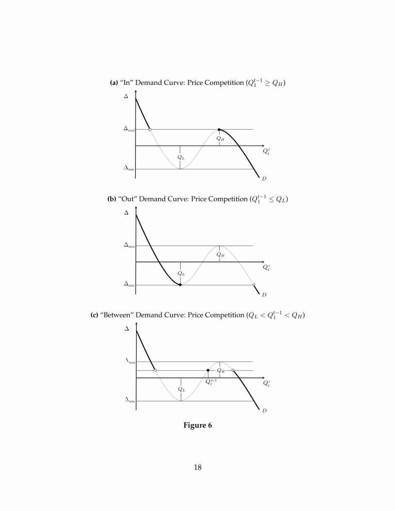
firm 1 faces one of the three negatively-sloped demand curves shown in Figure 6.
Corollary 3. In any period, firm 1 faces one of three downward-sloping demand curves
(depending upon Qt−11 ):
1. “In” Demand Curve (Qt−11 ≥ QH).
2. “Out” Demand Curve (Qt−11 ≤ QL).
3. “Between” Demand Curve (QL < Qt−11 < QH).
17
(a) “In” Demand Curve: Price Competition (Qt−11 ≥ QH )“In” Demand Curve: Bertrand Competition (Q
t–1 ≥ QH) 1
QH
QL
D
max
min
Q t 1
(b) “Out” Demand Curve: Price Competition (Qt−11 ≤ QL)“Out” Demand Curve: Bertrand Competition (Q
t–1 ≤ QL) 1
QH
QL
D
max
min
Q t 1
(c) “Between” Demand Curve: Price Competition (QL < Qt−11 < QH )“Between” Demand Curve: Bertrand Competition (QL < Q
t–1 < QH) 1
QH
QL
D
max
min
Q t 1
Q t–1 1
Figure 6
18
We will again refer to a firm as “in,” “out,” or “between” depending upon
whether it faces an “in,” “out,” or “between” demand curve. Because overall
demand is fixed (Q1 +Q2 = 1), either both firms are “between” or one is “in” and
the other is “out.”5
We will focus attention on the case where firm 1 starts “in” and firm 2 starts
“out.” This corresponds to many cases of interest, where competition is between
an established firm that has built up a network and a recent entrant.
3.2 Analysis
We are now in a position to formally state and analyze the pricing game played
by the firms.
At stage 1, firm 1 sets a price p1; at stage 2, firm 2 sets a price p2. The resulting
payoffs to the firms are π1 = p1·Qin1 (∆) and π2 = p2·(1−Qin
1 (∆)), where ∆ = p1−p2.
Observe that π1 and π2 depend upon the shape of the demand curve; the demand
curve, in turn, depends upon parameters α, µ, and F .
We can use backward induction to solve for the equilibrium of the game. Let
pBR2 (p1) denote firm 2’s best response to price p1 and let ∆(p1) = p1−pBR2 (p1). Firm
1 chooses p1 to maximize:
π1(p1) = p1 ·Qin1 (∆(p1)).
Firm 1 “remains in” if ∆(p1) ≤ pmax and “falls out” if ∆(p1) ≤ pmax. We will
refer to ∆(p1) ≤ pmax as the “remain-in constraint” or RIC. Demand for good 1
decreases discontinuously when firm 1 falls out. Hence, there is an incentive for
firm 1 to choose a price that satisfies RIC. Furthermore — and most importantly
— RIC will be a binding constraint in a region of the parameter space.
It is easy to show that, to remain in, firm 1 must set a price below a threshold
pRIC (the argument is given below as part of the proof of Proposition 4). Therefore,
5It might be possible for both firms to be “in” if overall demand were not fixed.
19

the following is an equivalent formulation of the remain-in constraint:
p1 ≤ pRIC(α, µ, F ). (RIC)
Proposition 4 characterizes how a change in the goods’ relative qualities (µ)
affects the equilibrium outcome in the region where RIC binds.
Proposition 4. When RIC binds, increases in the quality of good 1 relative to good 2, as
measured by µ:
1. Translate one-to-one into increases in good 1’s equilibrium price:
∂pRIC
∂µ= 1.
2. Have no effect on good 2’s equilibrium price.
3. Have no effect on equilibrium quantities (Q1 and Q2).
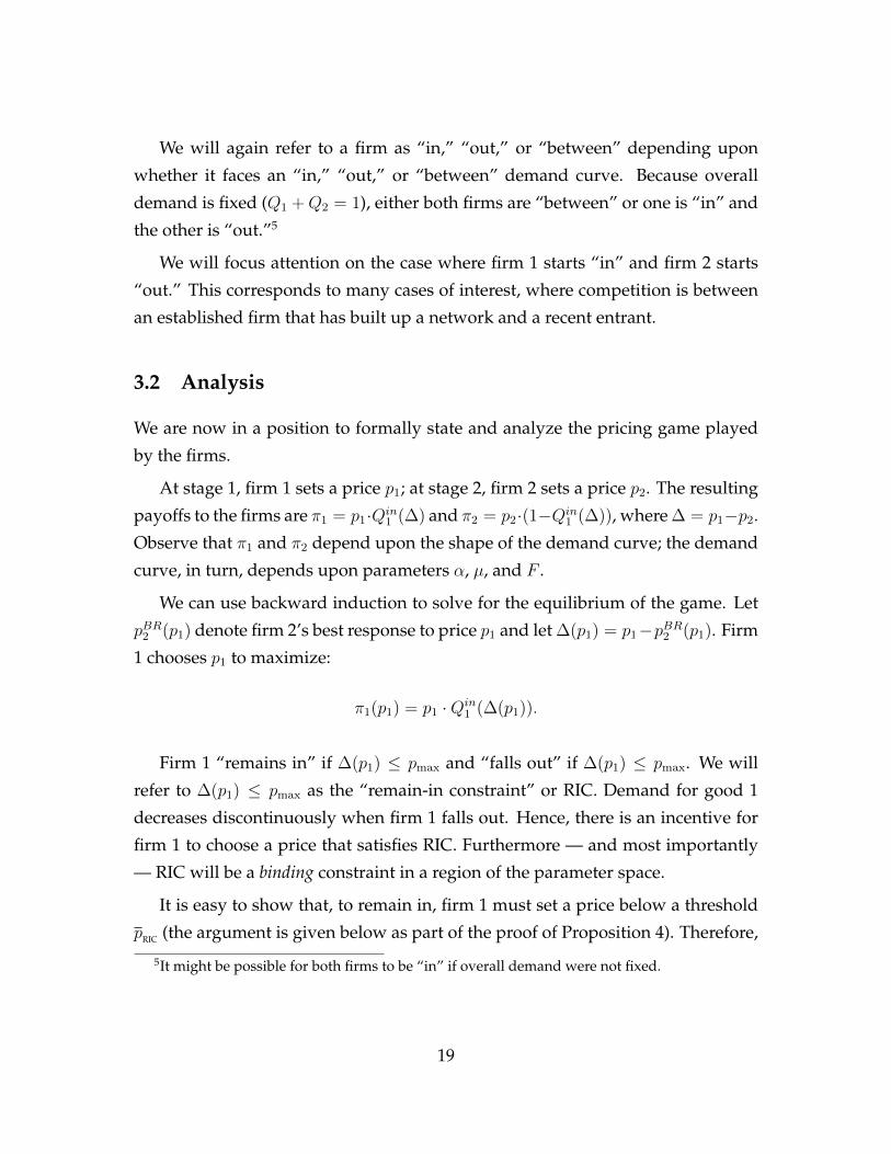
Proof of Proposition 4
Figure 7 shows the demand for good 2 for a particular value of p1. Firm 2’s
best response to p1 is either to choose:
1. The profit-maximizing price conditional on staying “out” (plocal in the fig-
ure).
2. The profit-maximizing price conditional on going “in.”
At least when firm 2 is on the margin between staying “out” or going “in,” pminwill be the profit-maximizing price conditional on going “in.”
The red region in Figure 7 represents the profits to firm 2 from choosing plocal;
the blue region represents the profits from choosing pmin. Observe that RIC is
satisfied when the red region is (weakly) larger than the blue region; RIC binds
when the regions are of equal size.
20
The Remain-In Constraint (RIC)
D’Q2
pmin
plocal
Higher p1
D
p2 (Q )d2
Lower μ
Q2
localQ2
min
Figure 7
An increase in p1 shifts firm 2’s demand curve vertically up, which increases
the size of the blue region relative to the red region.6 This explains why firm 1
must price below a threshold, pRIC, in order to meet RIC.
Suppose RIC is a binding constraint and suppose demand curve D in Figure 7
depicts the place where RIC exactly binds. Observe that the demand curve firm 2
faces depends upon the “effective price” of good 1: p1 − µ. Hence, if µ decreases
by an amount ∆µ, firm 1 must decrease p1 by ∆µ to stay on demand curve D.
This explains why, in the region where RIC binds, a change in µ changes p1 by
an equivalent amount. Furthermore, since firm 2 always faces the same demand
curve D in the region where RIC binds, it always charges the same price (plocal)
and sells the same quantity (Qlocal2 ). QED.
In practice, “in” firms may need to charge low — even zero — prices to sat-6The reason the blue region increases in size more than the red region when p1 increases is that
Qmin2 > Qlocal
2 .
21

isfy the RIC constraint. For example, despite their overwhelming market shares,
Google (in web search), Uber (in ride sharing), and Amazon Web Services (in
cloud computing) all keep their prices low — arguably to stunt the rise of their
nearest rivals.
3.3 Incentives for Innovation
The fact that when network externalities are large, the winning and losing firms
compete for the “in” position, as opposed to merely competing for a single marginal
consumer, has important implications for the firms’ incentives to innovate.
To illustrate, suppose the two firms have an opportunity to invest up front on
R&D activities that raise the intrinsic quality of their respective products. Let µidenote the intrinsic quality of firm’s i product, with µ = µ1 − µ2. Suppose quality
µi costs C (µi) to obtain, where C is twice differentiable and satisfies C ′, C ′′ > 0
and C ′ (0) = 0. Suppose µ1 and µ2 are observed by both firms before they engage
in price competition. (The exact timing of the choices of µ1 and µ2 is immaterial.)
Corollary 4 shows that, when the network externality is strong, the two firms
face radically different incentives to innovate:
Corollary 4. Consider the extended model with investments. Suppose firm 1 retains the
“in” position and suppose that, in the pricing stage, the remain-in constraint is binding
(that is, the network externality is large). Then:
1. Firm 1’s optimal investment µ∗1 satisfies
C ′ (µ∗1) = Q∗1,
where Q∗1 denotes the equilibrium sales of firm 1.
2. Firm 2 has zero incentive to innovate.
This result follows from the fact that when the remain-in constraint is binding,
we have dp1dµ
= 1. As a result, an increase in firm 1’s quality translates one-to-
one into an increase in its equilibrium price, and hence firm 1 invests in direct
22
proportion to the size of its own market (which, given its winning position, is
large). In contrast, an increase in firm 2’s quality translates one-to-one into an
reduction in its rival’s price; thus, this higher quality has zero impact on firm 2’s
revenues.
In practice, firms may also increase the quality of the products by means of
acquiring startups with valuable product innovations. Here too, competition for
the “in” position may lead to highly asymmetric outcomes. To illustrate, sup-
pose a third party (a “startup”) possesses an innovation and, prior to engaging in
price competition, firms 1 and 2 bid in a (second-price) auction to buy the startup.
Suppose the firm that acquires the startup adopts its innovation, and as a result
improves its quality by ∆µ.
In this setting, provided the hypothesis of Corollary 4 is met, firm 1’s maxi-
mum bid for the startup is 2∆µQ1; whereas firm 2’s maximum bid is 0.7 There-
fore, firm 1 acquires the startup and pays 0 for it, further cementing it dominant
position. In fact, in a multi-period version of this merger game in which a new
startup emerges in every period, the dominant firm outbids its rival for each new
startup; thus, its dominant position becomes more and more entrenched as time
goes by.
4 Piecewise Linear Demand
When consumers’ tastes follow a particular type of distribution (see Figure 8a),
the in/out demand curve is piecewise linear. Figure 8b depicts the in/out demand
curve for a monopolist firm corresponding to Figure 8a.
When demand is piecewise linear, we can solve explicitly for the outcome of
price competition. Furthermore, piecewise linear demand facilitates an analysis
of the effects of demand volatility.
7By winning, firm 1 not only increases its quality by ∆µ, it also prevents firm 2 from increasingits quality by ∆µ. Hence firm 1 is willing to bid 2∆µ per unit of expected sales (as opposed to ∆µ).
23

(a) Pdf that gives rise to piecewise linear demand.
a
b
a
b
(b) Corresponding demand curve for the monopoly case (demand is in/out if α > 1v1+v2
).
p
1
D
1-av22v1
-1+av22v1
+ α+ μ
Q
12
[-a + α(1+a(v1+v2)] + μ
12
[a + α(1-a(v1+v2)] + μ
+ μ
Figure 8
24
4.1 Demand Volatility
Suppose, as in Section 2, there is a monopolist and suppose there is just a single
pricing period (T = 1). Consumers’ tastes are distributed as in Figure 8a and the
network externalities are sufficiently large that demand is in/out (α > 1v1+v2
). In
contrast to Section 2, µ (the quality of the monopolist’s good relative to the outside
option) is a random variable: µ = µ̂+ ε, where:
ε =
σ, with probability r.
−σ, with probability r.
0 with probability 1− 2r.
The resulting demand curve, pd(Q), has a random component:
pd(Q) = p̂(Q) + ε.
We assume the monopolist is risk neutral.
How does demand volatility affect optimal pricing? Let p∗(σ) denote the opti-
mal price for a given level of volatility, σ. Let us focus attention on the case where
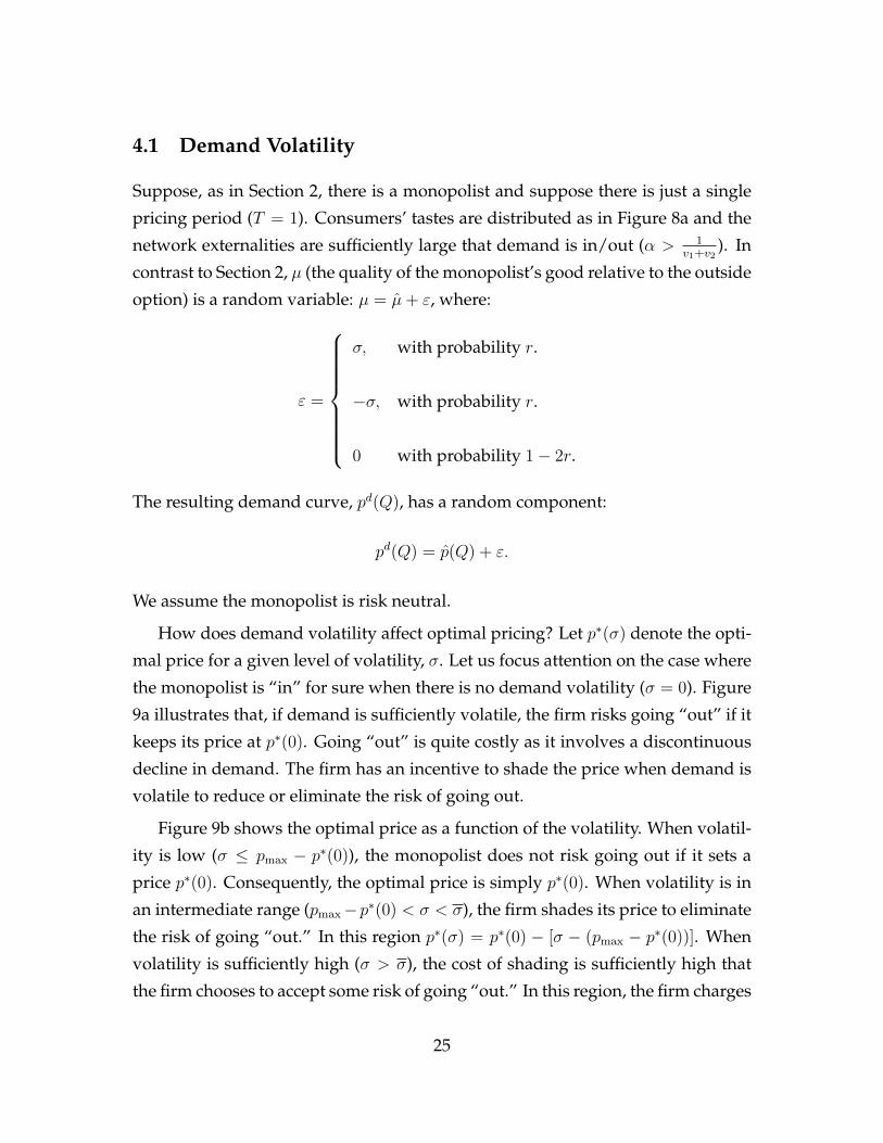
the monopolist is “in” for sure when there is no demand volatility (σ = 0). Figure
9a illustrates that, if demand is sufficiently volatile, the firm risks going “out” if it
keeps its price at p∗(0). Going “out” is quite costly as it involves a discontinuous
decline in demand. The firm has an incentive to shade the price when demand is
volatile to reduce or eliminate the risk of going out.
Figure 9b shows the optimal price as a function of the volatility. When volatil-
ity is low (σ ≤ pmax − p∗(0)), the monopolist does not risk going out if it sets a
price p∗(0). Consequently, the optimal price is simply p∗(0). When volatility is in
an intermediate range (pmax−p∗(0) < σ < σ), the firm shades its price to eliminate
the risk of going “out.” In this region p∗(σ) = p∗(0) − [σ − (pmax − p∗(0))]. When
volatility is sufficiently high (σ > σ), the cost of shading is sufficiently high that
the firm chooses to accept some risk of going “out.” In this region, the firm charges
25
(a) There is a risk the firm goes from “in” to “out” if σ > 0.
D
Q
p
p (0)*
D’
(b) Optimal pricing as a function of volatility (σ).
σ
p*(σ)
σpmax–p*(0)
p*(0)
p*(σ)
Figure 9
26
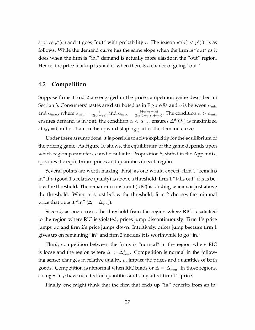
a price p∗(σ) and it goes “out” with probability r. The reason p∗(σ) < p∗(0) is as
follows. While the demand curve has the same slope when the firm is “out” as it
does when the firm is “in,” demand is actually more elastic in the “out” region.
Hence, the price markup is smaller when there is a chance of going “out.”
4.2 Competition
Suppose firms 1 and 2 are engaged in the price competition game described in
Section 3. Consumers’ tastes are distributed as in Figure 8a and α is between αmin
and αmax, where αmin = 12(v1+v2)
and αmax = 1+a(v1−v2)2v1(1+a(v1+v2))
. The condition α > αmin
ensures demand is in/out; the condition α < αmax ensures ∆d(Q1) is maximized
at Q1 = 0 rather than on the upward-sloping part of the demand curve.
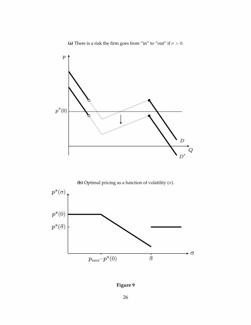
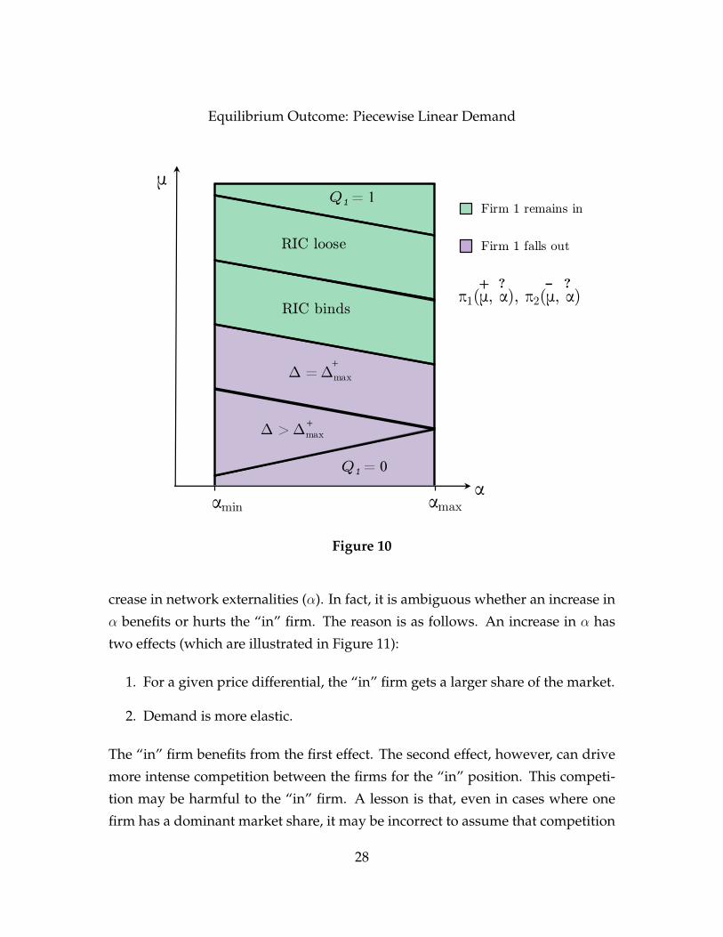
Under these assumptions, it is possible to solve explicitly for the equilibrium of
the pricing game. As Figure 10 shows, the equilibrium of the game depends upon
which region parameters µ and α fall into. Proposition 5, stated in the Appendix,
specifies the equilibrium prices and quantities in each region.
Several points are worth making. First, as one would expect, firm 1 “remains
in” if µ (good 1’s relative quality) is above a threshold; firm 1 “falls out” if µ is be-
low the threshold. The remain-in constraint (RIC) is binding when µ is just above
the threshold. When µ is just below the threshold, firm 2 chooses the minimal
price that puts it “in” (∆ = ∆+max).
Second, as one crosses the threshold from the region where RIC is satisfied
to the region where RIC is violated, prices jump discontinuously. Firm 1’s price
jumps up and firm 2’s price jumps down. Intuitively, prices jump because firm 1
gives up on remaining “in” and firm 2 decides it is worthwhile to go “in.”
Third, competition between the firms is “normal” in the region where RIC
is loose and the region where ∆ > ∆+max. Competition is normal in the follow-
ing sense: changes in relative quality, µ, impact the prices and quantities of both
goods. Competition is abnormal when RIC binds or ∆ = ∆+max. In those regions,
changes in µ have no effect on quantities and only affect firm 1’s price.
Finally, one might think that the firm that ends up “in” benefits from an in-
27
Equilibrium Outcome: Piecewise Linear Demand
μ
Q1 = 0
Δ >Δmax
α
+
Q1 = 1
RIC binds
RIC loose
Δ =Δmax
αmaxαmin
+
Firm 1 remains in
π1(μ, α), π2(μ, α)+ ? – ?
Firm 1 falls out
Figure 10
crease in network externalities (α). In fact, it is ambiguous whether an increase in
α benefits or hurts the “in” firm. The reason is as follows. An increase in α has
two effects (which are illustrated in Figure 11):
1. For a given price differential, the “in” firm gets a larger share of the market.
2. Demand is more elastic.
The “in” firm benefits from the first effect. The second effect, however, can drive
more intense competition between the firms for the “in” position. This competi-
tion may be harmful to the “in” firm. A lesson is that, even in cases where one
firm has a dominant market share, it may be incorrect to assume that competition
28
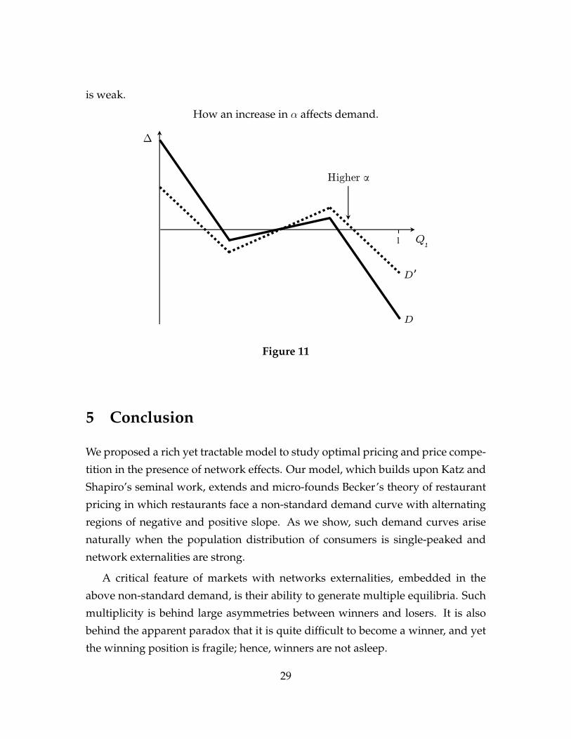
is weak.
How an increase in α affects demand.
Δ
1
D
D’
Q1
Higher α
Figure 11
5 Conclusion
We proposed a rich yet tractable model to study optimal pricing and price compe-
tition in the presence of network effects. Our model, which builds upon Katz and
Shapiro’s seminal work, extends and micro-founds Becker’s theory of restaurant
pricing in which restaurants face a non-standard demand curve with alternating
regions of negative and positive slope. As we show, such demand curves arise
naturally when the population distribution of consumers is single-peaked and
network externalities are strong.
A critical feature of markets with networks externalities, embedded in the
above non-standard demand, is their ability to generate multiple equilibria. Such
multiplicity is behind large asymmetries between winners and losers. It is also
behind the apparent paradox that it is quite difficult to become a winner, and yet
the winning position is fragile; hence, winners are not asleep.
29

Understanding markets with network externalities therefore requires under-
standing how consumers pick one equilibrium over another. To this end, we pro-
posed a simple theory of equilibrium selection (formally, introspective equilibrium)
that captures the notion that a firm’s popularity exhibits a form of inertia over
time, and is affected as well by salient consumers that are popular among their
peers. A firm’s default popularity, inherited from the previous period, then deter-
mines whether it currently faces its worst possible demand curve (the “out” de-
mand), its best possible curve (the “in” demand), or an intermediate version of the
two (the “between” demand). Each of these demand curves has a well-behaved
shape with a standard negative slope but with a discontinuity. This simple clas-
sification immediately sheds light on the firm’s optimal pricing, its equilibrium
transitions between the losing and the winning positions, and its incentives for
innovation.
Our model features a form of asymmetric competition in which a winning and
losing firm co-exist, with the losing firm keeping the winning firm in check. We
show that this check on the winning firm is a generalized form of “limit pricing,”
whereby a monopolist is disciplined by a potential entrant.8 In our case, rather
than deterring entry outright, the winning firm needs to deter the losing firm
from becoming popular. It does so by allowing the losing firm to enjoy rents from
a small but loyal consumer base, a form of consolation prize.
In subsequent work, we expect to propose a method for valuing firms in the
presence of network effects, with such effects opening the possibility of large prof-
its for popular firms, but also to inevitable risks of sudden failure.
8For classic references on limit pricing, see Gaskins (1971) and Milgrom and Roberts (1982).
30

6 Appendix
Proposition 5. The equilibrium of the pricing game depends upon which region parame-
ters µ and α fall into. There are six regions which can be ordered from a highest-µ region
to a lowest-µ region:
1. RIC is loose and Q∗1 = 1 (µ ≥ µ1):
p∗1 = µ+ α +−1 + av2
2v1
.
p∗2 = 0.
2. RIC is loose and Q∗1 < 1 (µ1 > µ ≥ µ2):
p∗1 =1
2µ− 3
2α +
3 + av2
4v1
.
p∗2 = −1
4µ− 5
4α +
5− av2
8v1
.
Q∗1 =v1
2(1− 2v1α)(1
2µ− 3
2α +
3 + av2
4v1
).
3. RIC binds (µ2 > µ ≥ µ3):
p∗1 = µ+ α(2a(v1 + v2)− 1) +a(3v2 − 2v1) + 1
2v1
− 2
v1
√av2[
1
2(1 + a(v2 − v1))− αv1(1− a(v1 + v2))].
p∗2 = α(a(v1 + v2)− 1) +a(v2 − 2v1) + 3
4v1
− 1
v1
√av2[
1
2(1 + a(v2 − v1))− αv1(1− a(v1 + v2))].
Q∗1 =1− a(v2 − v1)
2(1− 2v1α)− αv1(a(v1 + v2) + 1)
1− 2v1α
+1
1− 2v1α
√av2[
1
2(1 + a(v2 − v1))− αv1(1− a(v1 + v2))].
31
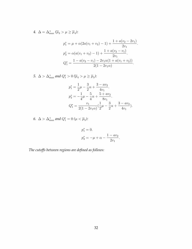
4. ∆ = ∆+max (µ3 > µ ≥ µ4):
p∗1 = µ+ α(2a(v1 + v2)− 1) +1 + a(v2 − 2v1)
2v1
.
p∗2 = α(a(v1 + v2)− 1) +1 + a(v2 − v1)
2v1
.
Q∗1 =1− a(v2 − v1)− 2v1α(1 + a(v1 + v2))
2(1− 2v1α).
5. ∆ > ∆+max and Q∗1 > 0 (µ4 > µ ≥ µ5):
p∗1 =1
2µ− 3
2α +
3− av2
4v1
.
p∗2 = −1
4µ− 5
4α +
5 + av2
8v1
.
Q∗1 =v1
2(1− 2v1α)(1
2µ− 3
2α +
3− av2
4v1
).
6. ∆ > ∆+max and Q∗1 = 0 (µ < µ5):
p∗1 = 0.
p∗2 = −µ+ α− 1− av2
2v1
.
The cutoffs between regions are defined as follows:
32
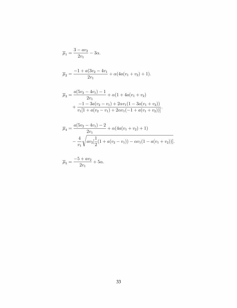
µ1 =3− av2
2v1
− 3α.
µ2 =−1 + a(3v2 − 4v1
2v1
+ α(4a(v1 + v2) + 1).
µ3 =a(5v2 − 4v1)− 1
2v1
+ α(1 + 4a(v1 + v2)
+−1− 3a(v2 − v1) + 2αv1(1− 3a(v1 + v2))
v1[1 + a(v2 − v1) + 2αv1(−1 + a(v1 + v2))].
µ4 =a(5v2 − 4v1)− 2
2v1
+ α(4a(v1 + v2) + 1)
− 4
v1
√av2[
1
2(1 + a(v2 − v1))− αv1(1− a(v1 + v2))].
µ5 =−5 + av2
2v1
+ 5α.
33

References
Akerlof, Robert and Richard Holden, “Capital Assembly,” CEPR Discussion Paper
No. 11763, 2017.
Autor, David, David Dorn, Lawrence F. Katz, Christina Patterson, and John Van
Reenen, “The Fall of the Labor Share and the Rise of Superstar Firms,” CEPR
Discussion Paper No. 12041, 2017.
Becker, Gary S., “A note on restaurant pricing and other examples of social influ-
ences on price,” Journal of Political Economy, 1991, 99 (5), 1109–1116.
Cain Miller, Claire, “Browser Wars Flare Again, on Little Screens,” The New York
Times, December 9, 2012.
Gaskins, Darius W., “Dynamic limit pricing: Optimal pricing under threat of
entry,” Journal of Economic Theory, 1971, 3, 306–322.
Katz, Michael L. and Carl Shapiro, “Network externalities, competition, and
compatibility,” The American Economic Review, 1985, 75 (3), 424–440.
and , “Systems competition and network effects,” The Journal of Economic
Perspectives, 1994, 8 (2), 93–115.
Milgrom, Paul and John Roberts, “Limit Pricing and Entry under Incomplete
Information: An Equilibrium Analysis,” Econometrica, 1982, 50 (2), 443–459.
Rivkin, Jan W. and Eric J. Van den Steen, “Microsoft’s Search,” Harvard Business
School Case 709-461, 2009.
Yoffie, David B. and Michael A. Cusumano, Competing on Internet time: lessons
from Netscape and its battle with Microsoft, Simon and Schuster, 1998.
34