Embed Size (px)
Citation preview

1
Vehicle Emissions and Life Cycle Analysis Models
of Gasoline and Electric Vehicles
Corey M. Walker and Aly M. Tawfik, Ph.D. (Corresponding Author),
Department of Civil and Geomatics Engineering, California State University, Fresno
2320 E. San Ramon Ave. M/S EE94, Fresno, CA 93740
([email protected] and [email protected])
ABSTRACT
In addition to air pollution emissions, the transportation sector in the US is responsible
for more than 25% of greenhouse gas emissions. Due to the negative impacts of these emissions,
primarily on health and the environment, literature of vehicle emissions models is rich. Yet,
attempts to synthesize and contrast models of this rich literature are scarce. Contrasting models
of gasoline and electric vehicle emissions could be particularly beneficial due to the significant
differences between these two technologies; specifically with respect to emissions. Accordingly,
this paper adopts a life cycle analysis approach to synthesize and explore the development and
structure of some of the most common emissions models. The paper starts with a brief discussion
of the emission models measurement techniques; then, explores and contrasts state-of-the-art
vehicle emissions models. Four groups of emissions models are included in this synthesis: 1)
Macro-scale models: MOVES2014 and EMFAC; 2) Meso-scale models: VT-Meso,
MOVES2014, and MEASURE; 3) Micro-scale models: VT-Micro and CMEM; and 4) Electric
lifecycle models: MOVES2014 and GREET. The paper highlights the effects of lifecycle
analyses of both gasoline and electric vehicles on estimates of vehicle greenhouse gas emissions
from each of these two technologies. The paper ends with a discussion of the shortcomings of
current vehicle emissions models, limitations of their usage and application, and suggestions for
future work.
1. INTRODUCTION
Over the last 60 years, the concern over greenhouse gas (GHG) emissions has increased.
According to the United States Environmental Protection Agency (EPA), in 2012 28% of GHG
emissions were produced by the transportation sector.1 Beginning with the work of Arie J.
Haagen-Smit in 1948, significant gains have been made in understanding the major sources of
these emissions.2 In 1963 the United States Congress passed the Clean Air Act, providing the
framework for the first emissions control. Over the next 23 years, the Clean Air Act was
amended and updated to account for developing research and technology. 3 This legislation
requires in part that vehicle emissions models be created and subsequently updated to aid in the
estimation and controlling of emissions. Large efforts have now been made to model how
vehicles produce these emissions for the ultimate purpose of making vehicles more efficient.
Vehicle emissions models can be split into four main categories: macro, micro, meso, and life
cycle. The following sections present the prominent models that are found in current literature
for each of these categories. This paper is organized as follows: Section 2 contains a brief
discussion of various vehicle emissions data acquisition techniques. Section 3 discusses the
various vehicle emissions models used for the macro, micro, and meso categories, specifically

2
focusing on the approaches used in vehicle emissions predictions as well as strengths and
weaknesses of each model. Section 4 expands this discussion into life-cycle analysis models,
noting the affects this type of analysis has on emissions. The paper then ends with some
concluding remarks and recommendations for future work.
2. VEHICLE EMISSIONS DATA ACQUISITION
2.1 LABORATORY DATA ACQUISITION
Nearly every emissions model is created based on a combination of laboratory and field
measurements. In laboratory tests, vehicle emissions for various makes and models of vehicles
are measured using a chassis dynamometer. This tool connects directly to the engine’s crankshaft
and provides resistance either through a magnetic field or a water chamber. Dynamometers can
be calibrated to offer a specific amount of resistance to simulate factors such as friction, wind,
and sloped surfaces. During the test, the engine is run under a specific load cycle - a
predetermined sequence of accelerations, cruises, and idle periods. While the test is running,
emissions produced by the engine are collected and analyzed.4, 5
Laboratory tests are done in a controlled environment and allow vehicles of different
makes and models to be subjected to the same loading situations. This in turn produces results
that are relatively easy to compare and correlate. However, laboratory tests suffer from a major
flaw. They often misrepresent short-term events such as rapid accelerations and unusual driver
behavior. To solve this problem, many models also use field measurements to supplement data
obtained in the lab.
2.2 FIELD DATA ACQUISITION
Field measurements are done using On-board Emissions Measurement Systems (OEMS).
These systems connect to the vehicle tailpipe and the On-Board Diagnostic System (OBD).6
Emissions are collected from the tailpipe and the instantaneous speed and acceleration are
recorded through the OBD. OBDs come in various sizes depending on the type of vehicle being
analyzed. These proportions range from the size of a large backpack to the size of a small car.
Other measurement methods include power-train tests and remote sensing techniques.3
3. EMISSIONS MODELS
As stated above, vehicle emissions models can be split into four main categories: macro-,
meso-, and micro-scale, as well as life cycle analysis. Each of the first three scales encompasses
a certain scope. Marco models examine regions of area in a transportation system. These models
are not concerned so much with individual emissions from vehicles, but with the target area as a
whole.7, 8 Micro models are the opposite and focus on emissions from vehicles on an
instantaneous basis based on the speed and acceleration of the vehicle.7-9 Most often, they are
used to predict the amount and nature of the emissions at specific points or intersections along
transportation links. Meso models are a mixture of these two and typically involve a specific link
or traffic analysis zone of the transportation system.7, 8 During the development of these models,
the type of data required depends on the model and on the eventual purpose of the analysis. In
Commented [CL1]: Figure
Commented [CL2]: Figure
Commented [CL3]: Figure
Commented [CL4]: Expand on these

3
this section, the design of macro models will be discussed and will be expanded in the following
subsections to address micro and meso models.
3.1 MACRO VEHICLE EMISSIONS MODELS
Macro vehicle emissions models have historically been the fastest and simplest way of
obtaining estimates of vehicle emissions. Macro models require far less data inputs than other
scales, and due to their relatively basic structure and straightforward way of calculating
emissions, they are able to quickly return estimates. Though there are a large number of models
that are currently used, this paper will focus on the two major models found in literature: the
MOVES and EMFAC models.
3.1.1 MOVES MODEL
Beginning in 1970, the United States EPA began developing a macro vehicle emissions
model to serve as a tool when evaluating whether states or agencies were conforming to
provisions of the Clean Air Act.10 The EPA currently uses two macro emissions models: the
MOBILE model and its replacement, the MOtor Vehicle Emissions Simulator (MOVES).
Because the MOVES model has replaced the MOBILE model, the design of the MOVES model
will be discussed here. The MOBILE model still serves as a base platform for many countries
seeking to establish their own macro emissions model, but the development of the MOBILE
model is not significantly different from the MOVES model. As noted above, macro models deal
with large geographic areas and so do not require instantaneous speed and acceleration data.
Instead the MOVES model operates on what the EPA calls “total activity”. To calculate this
parameter, the MOVES model first divides vehicle uses into categories, using terrain (e.g.
rolling, flat) and location characteristics (e.g. urban, rural). Next, the vehicles being analyzed are
sorted into each of these usage categories. Finally, the model calculates how long each of these
vehicles spends traveling while in their given category.7 Using this approach, vehicles that have
long commutes will have a greater total activity than those with short commutes. Also, vehicles
that travel in rough terrain will have greater total activity than those is mild terrain.
The total activity calculations are primarily based on data that the EPA has itself
collected over decades of testing vehicles and from other agencies such as the California Air
Resources Board and various automobile manufacturers. This data is subdivided into various
categories based on the make and model of the vehicle as well as the model year. Additional
attributes of the data include terrain location and operating time.11
Notice, however, that in the EPA’s definition of total activity that the terminology is “the
population” of a given vehicle/use type. This refers back to the fact that MOVES used to
primarily be a macro-scale model, utilizing a large number or population of vehicles. It involves
a direct relationship between total activity and total emissions. The more activity a vehicle
undergoes, the more emissions are produced. For counties and large areas, this is an ideal type of
analysis. It is too expensive in most cases to collect emissions data for every type of vehicle
traveling in a region. Instead, the percent distribution of vehicle types and terrain can be
determined through such things as existing databases or vehicle registration information. This
Commented [CL5]: Expand on MOBILE

4
information can then be used in the MOVES model which will link the information with
previously tested vehicles of the same make and model that travelled over similar terrain.
This process is best illustrated by an example input into the model. Suppose a user wants
to determine the emissions in a particular city having a population of 200,000. From the city’s
vehicle registration information, it is discovered that passenger car model years range from 1968
to 2015 and that vehicle makes range between 12 different manufacturers. The terrain of the city
is primarily asphalt paving having average speed limits between 20-45 mph. The user can simply
determine distributions for each of these areas and input the data into the MOVES model. For
instance, perhaps 10% of the cars are 1968-1975 models, 24% are 1976-1987 models, 39% are
1988-2000 models, and 27% are 2001-2015 models. Furthermore, suppose that the car
population is equally distributed between the different manufacturers and between the different
speed ranges. Each of these distributions is linked to past data for that particular make,
manufacturer, model year, speed, etc. Combining all this data, the total emissions are then
calculated.
3.1.2 EMFAC MODEL
Another macro-scale model currently in use is the California Environmental Protection
Agency, Air Resources Board’s (CARB) EMission FACtors Model (EMFAC). This model is
structured in many ways like the MOVES model. Drawing from a large database obtained from
Department of Motor Vehicle records, Smog Check reports, and other sources, the EMFAC
model uses this information to calculate emissions factors that are multiplied by the source
activity of a vehicle. The processes behind these calculations are identical to those used in the
development of the MOVES model. During the creation of the EMFAC model, data regarding
each vehicle process of concern was evaluated and a correlation was made. Using this
correlation, the emissions for a given vehicle can be predicted, just as in the MOVES model.12
The major differences between the MOVES and EMFAC models are in their structure
and scope. The MOVES model is intended for use as a comprehensive, single unit. The EMFAC
model, on the other hand, is a composition of several smaller modules. The modules currently
divide the model into three portions: light-duty vehicle analysis, heavy-duty vehicle analysis, and
transportation planning analysis. By splitting up these functions, the EMFAC model both
provides a more direct approach to analysis and also allows its developers to easily add new
modules in the future should the need arise.13
Macro models are best when dealing with large populations of vehicles. Nevertheless, an
interesting and powerful function of the MOVES and EMFAC models is that they can be used to
predict vehicle emissions on both the meso and micro-scales. The same process that is described
above can be used for intersection and street level analyses simply by using a different
distribution of vehicle makes, models, and roadway speeds.
3.2 MICRO VEHICLE EMISSIONS MODELS
The necessity of having a micro vehicle emissions model began in 1990 with the passage
of a set of amendments to the Clean Air Act. These amendments required in part that

5
organizations provide plans that detail the impacts of transportation projects and improvements
on air quality. Signalized intersections, highway on-ramps, and other small scale projects
suddenly required a means of estimating future emissions.
Two micro emissions models came into being to fill this need. These were the
Comprehensive Modal Emissions Model (CMEM), developed by the University of California,
Riverside, and the Virginia Tech Microscopic energy and emissions model (VT-Micro). Both of
these models accomplish the same relative purpose, but tackle the problem in slightly different
ways.
3.2.1 THE COMPREHENSIVE MODAL EMISSIONS MODEL (CMEM)
The CMEM model was developed by the University of California, Riverside to predict
emissions for light-duty vehicles (i.e. automobiles and small trucks) under various operating
conditions.14 It is one of the most widely used micro-scale models and was created by breaking
the vehicle operation and emissions cycles into six categories: engine power, engine speed, air-
to-fuel ratio, fuel use, engine-out emissions, and catalyst pass fraction.11 The calculation of
emissions from each of these categories is determined using variables such as the vehicle speed
and acceleration and the grade of the roadway. This information is potentially available from
sources such as the EPA database. The emissions calculations also use constants in the form of
calibrated parameters. These include such things as the engine friction factor and cold start
coefficients.15 These constants are preset to default values in the core model, but can easily be
adapted to fit the context and particular parameters of a given situation.
During the development of the CMEM model, over 300 vehicles were tested in the
laboratory on a second-by-second basis using three different drive cycles. Both engine-out
emissions (emissions originating directly from the engine) and tailpipe emissions were
measured.15 This data was used to create a power-based model, basing emissions off of the
predicted power usage of the vehicle. The CMEM model calculates emissions using the process
illustrated in the following figure.
3.2.2 THE VIRGINIA TECH MICROSCOPIC ENERGY AND EMISSIONS MODEL
(VT-MICRO)
The VT-Micro model was originally developed in the early 1990s using emissions data
from nine light duty vehicles. In 2002, this data set was expanded to include tests from 60
vehicles.11 Like the CMEM model, inputs to the VT-Micro model include the instantaneous
speed and acceleration of the vehicle. However, the VT-Micro model uses a non-linear
regression structure in place of a power-demand model. One of the major defects of the CMEM
model is that it returns the same emissions estimate for situations in which the amount of applied
power is the same. For example, a vehicle may use the same amount of power driving 60 mph in
flat terrain as it would driving at 20 mph on a steeply sloped road. The actual emissions produced
in these situations may be very different, but since the CMEM model uses power to calculate
emissions it returns the same emissions estimate for both cases. Using a regression analysis, the
VT-Micro model solves this problem by relating emissions estimates to the instantaneous speed
and acceleration of the vehicle, rather than to power.

6
Another problem with the CMEM model was that it estimated a constant amount of
emissions whenever a vehicle experienced negative acceleration. As has been shown in
numerous tests, the emissions curve is in fact variable during these decelerations. To address this
issue, developers of the VT-Micro model used two separate mathematical formulae to estimate
emissions – one for positive accelerations and another for negative accelerations. These formulae
have the same form and vary only in the regression coefficients used. 9
It is important to note that while the CMEM model takes into account the vehicle
operating condition, such as the power demand and condition of the engine, air/fuel ratios, and
enrichment and enleanment conditions, the VT-Micro model has no such analysis, relying
instead on empirical data that leads to generalizations and simplified processes. This is both a
benefit and a disadvantage of the VT-Micro model. The benefit is that the VT-Micro model is
much simpler in its structure and abnormal emissions behavior can easily be traced back to the
source. The disadvantage is that in situations where the vehicle is in disrepair (e.g. deteriorated
or malfunctioning engine), the VT-Micro model may underestimate the emissions produced.11
3.2.3 MOVES AND EMFAC MODELS
As noted earlier, both the MOVES and EMFAC models have the capability to be used in
micro emissions models. The approach used in each of these models is the same as that used in
the macro-scale analysis. The only difference is in the input parameters required. For instance,
when the MOVES model is used for macro-scale analysis, instantaneous data is ignored and
average speeds and distances are used instead. When used in micro-scale analysis, however, the
instantaneous speed and acceleration of a vehicle are necessary inputs. Nevertheless, the process
that each model goes through to estimate emissions on a micro-scale is exactly the same as that
discussed earlier in Section 3.1.
3.3 MESO VEHICLE EMISSIONS MODELS
Every model is originally designed to serve a specific purpose. For macro-scale
emissions models, the goal was to provide estimates for large geographical areas using easily
obtained data. Micro-scale models came about with the advent of traffic simulation programs and
the Clean Air Act Amendments of 1990. The need arose to model emissions accurately on a
small scale for a particular intersection, ramp, or roadway. In many cases, though, there is either
an inability to collect enough data for a microscopic analysis or a lack of time to collect and
evaluate this data. In these situations, macro models were used to model the emissions, but this
resulted in estimates heavily prone to error. The macro models simply did not have enough
parameters to accurately predict the emissions on a microscopic scale. Researchers began to
merge the macro and micro models together, forming models that were less data intensive then
micro models, but still maintained a high level of accuracy for small scale analysis. There are
currently three main meso models mentioned repeatedly throughout literature, the VT-Meso, the
MOVES model previously mentioned, and the MEASURE model.
3.3.1 THE VIRGINIA TECH MESO MODEL

7
The VT-Meso model uses an approach similar to the VT-Micro model, estimating
emissions using a non-linear regression model. However, instead of the basic input parameters
being instantaneous speed and acceleration, in the VT-Meso model the basic inputs are average
vehicle speed, number of stops made, and stopped delays for a given link or intersection. Using
these inputs, the model creates a synthetic drive cycle and determines the amounts of time a
vehicle would spend accelerating, decelerating, idling, and cruising. These values are then used
in a series of mathematical formulae that allow the user to predict the amount of fuel
consumption and emissions produced.16
3.3.2 THE MOVES 2014 MODEL
The MOVES 2014 model uses a different approach to estimate emissions on a meso-
scale. As discussed in previous sections, this model is also commonly used in macro-scale
analysis. Its approach to both scales is the same. In both macro and meso-scale analysis, the
MOVES model separates the vehicles operation into different operating modes based on a wide
variety of parameters including speed, acceleration, and road grade. Once this is done, the total
activity of the vehicle is calculated and then compared with historical data. Using this
comparison, estimates are made for the amounts of emissions produced. Additional input
parameters that are required for meso-scale analysis (in addition to those required for macro-
scale analysis) include vehicle miles travelled (VMT), road type, age of the vehicle, speed
distribution, meteorological data, and vehicle type. 11, 16 These extra parameters help the model
generate more accurate estimates for the vehicle’s emissions.
3.3.3 THE MEASURE MODEL
The Mobile Emission Assessment System for Urban and Regional Evaluation
(MEASURE) model uses an empirical statistical approach to estimating emissions. Originally
created for use with GIS systems, the MEASURE model uses vehicle registration data, travel-
demand forecasts of flows, speed and acceleration distribution tables, and socioeconomic data as
inputs. From these the model can predict congestion levels and the distribution of modal
activities. Finally, the model uses these values to create emissions estimates for each link or zone
being evaluated. In many ways, the approach of the MEASURE model is comparable to the
MOVES model. Both separate vehicle activities into various operating modes and then use
comparisons with past data to generate emissions estimates. The advantage of the MEASURE
model, however, is that it is less biased than other models. Because its approach is statistical, it
chooses the most probable values for emissions estimates, rather than averages or most
frequently occurring values.17
3.3.4 COMPARISON OF MESO MODELS
All three of these models have their own set of advantages and disadvantages. The VT-
Meso model requires very few inputs and is therefore a relatively simple model to use. In
addition, it was calibrated to return the same emissions estimates as the VT-Micro model for a
given vehicle. Because of this, there exist strong correlations between the VT models. A
significant disadvantage of the VT-Meso model, though, is that it assumes constant accelerations
and decelerations throughout the drive cycle (Figure 2). Careful efforts have been made to ensure

8
that despite the obvious differences between the actual and synthetic drive cycles, they are equal
in terms of fuel consumption and emissions produced. Nevertheless, because of the averaging
process involved in this model, it may under or overestimate emissions for erratic driving
behavior situations.
The EPA’s MOVES model’s strength lies in its extensive inventory and database
information. It has the ability to estimate emissions for dozens of vehicle modes (which are
determined – among other things – by speed, acceleration, and road grade), providing far more
flexibility than other models. In fact, its inventories of data are used by nearly every research
facility developing new emissions models in the United States. The MOVES model has an easy-
to-use interface and requires data that can be obtained from a traffic demand model of the area in
question. The problem with the MOVES model is that it uses a comparative process for
emissions – taking data from tests of similar vehicles and using that data in equations that model
vehicle operating processes.18 While this makes the model very efficient for most vehicle
scenarios, it also causes the model to have trouble in accurately predicting emissions for
situations in which there are significant amounts of time spent in acceleration and deceleration.
In these situations, the VT-Meso or MEASURE models would be better choices for emissions
estimation. Keep in mind, however, that the MEASURE model was specifically designed for use
with a GIS database.16 In order to take advantage of the MEASURE model’s statistical approach,
source data may have to be converted into an acceptable format.
4. LIFE CYCLE ANALYSIS
Life cycle analyses (LCAs) came into existence long before the creation of vehicle
emissions models. This type of analysis examines the entire life of the vehicle, beginning with
the extraction of the fuel source and continuing through the manufacture, use, and disposal of the
vehicle. Though life cycle analyses are used for a broad range of applications, for the purpose of
this paper we will limit our discussion to life cycle analysis as it applies to modeling vehicle
emissions for both gasoline and electric vehicles. In vehicle emissions modeling, the life cycle
analysis process covers five main areas: raw material acquisition/procurement, material
processing, vehicle assembly, vehicle service life or use of the vehicle, and the recycling/disposal
of the vehicle, as shown below (Figure 3). 19 These areas are examined briefly below.
4.1 OVERVIEW OF VEHICLE EMISSIONS LIFE CYCLE ANALYSIS
The raw material extraction phase of a LCA involves determining the amount of
emissions generated by the collection of fuels, metals, chemicals, and other resources as they
exist in their natural state in, on, or above the earth. After their extraction, these materials are
then transported to industrial facilities. Once the raw materials reach the industrial facilities, they
enter the materials production phase in which they are refined and processed for subsequent use
in the construction of the vehicle. Also included in this phase are the production of batteries,
engines, motors, and the generation of fuel or electricity. The next phase in LCAs is vehicle
production. This phase could perhaps be better labeled as vehicle assembly and testing as it
involves the actual construction of the vehicle using the materials produced in the previous
phase. Following this is the service life of the vehicle. This is itself a collection of other
subgroups including the maintenance, use, and storage of the vehicle. Many life cycle studies

9
end their analysis after this phase, choosing to ignore the disposal or recycling of the vehicle
components because of the variability of emissions involved in this last phase. This type of study
is a subset of LCAs and is commonly called a “Well-to-Wheels Analysis”. LCAs that do include
the final phases treat recycling as the removal of any parts or components that can be reused or
salvaged. Most of these recycled materials are reincorporated into the materials production phase
as shown in Figure 3. For all of the components that are either too expensive or impossible to
recycle, such as vehicle batteries, the only option left is to dispose of them. This constitutes the
final phase of LCAs and though often ignored, can greatly affect the long term sustainability of a
particular design or solution.
LCA models in literature are not consistent. As mentioned above, though a
comprehensive LCA model should include all five stages, most do not. For example, in addition
to “Well-to-Wheels Analyses”, researchers will also refer to a “Pump-to-Wheels Analysis”, also
called a “Tank-to-Wheels Analysis”. This also is not a true life cycle analysis and only examines
the service life phase. Beginning with the moment fuel is pumped into a vehicle, the emissions
are measured and recorded. It is this type of analysis that is currently used when modeling
gasoline vehicle emissions. All of the emissions models discussed so far have been “Tank-to-
Wheels” analyses and as has been shown the models differ both in their scope and in their
approach to modeling in-vehicle emissions for gasoline vehicles.
When constructing electric vehicle emissions models, the standard approach of using a
Tank-to-Wheels analysis is not as beneficial. Though Tank-to-Wheel studies are still used to
determine in-vehicle emissions, these analyses are mostly done as part of an LCA. The necessity
for using a LCA is that electric vehicles essentially produce no tailpipe emissions. The service
life of an electric car therefore produces only a very small effect on the overall emissions
produced by electric vehicle. The primary LCA model found in literature is the GREET model. It
is important to note that although some models such as MOVES and EMFAC can evaluate
emissions from electric or hybrid vehicles, they can only evaluate the service life phase. The
GREET model is therefore the only model addressed in this paper that performs a full LCA.
4.2 THE GREET MODEL
The foremost and most significant life cycle analysis model for both electric and gasoline
vehicles is the GREET Model, developed by the U.S. Department of Energy at the Argonne
National Laboratory. Much like the MOVES model discussed earlier, the GREET model
calculates emissions using factors determined based on the pathway being analyzed. In this case,
a pathway can be best defined by an example. Taking the six stages of a LCA, imagine that the
lithium for a battery was extracted by a mining process, was transported by truck to a refining
plant, and was then refined using electrolysis. Next, suppose that the refined lithium is used to
construct a lithium-ion battery that will be later installed in a vehicle. Once the installation is
complete, the finished vehicle is transported by air and then truck to a sales location where it is
sold. The vehicle is then used for many years until it is no longer functional. Each of these steps
of the LCA together make up a single pathway. If even just one phase of the LCA was changed,
such as transporting the raw material by freight train instead of truck, then it would result in a
completely different pathway.

10
As can be seen, there is a vast multitude of possible pathways that the GREET model
uses. The materials transportation phase alone can happen in many different ways, such as
through the use of trucks, rail cars, ocean liners, barges, air freight, or pipelines.20 In the GREET
model, each of these travel modes has a separate emissions factor associated with it. In the same
way, each manufacturing process has a separate emissions factor associated with it. This method
of analysis is repeated through all the different aspects of the vehicle pathway, with each phase
yielding a separate emissions factor. These emissions factors are then combined and used to
calculate the total emissions produced during the life of the vehicle.
It is important to draw a distinction at this point between the gasoline vehicle emissions
models discussed in Section 2 of this paper and the GREET model. Previously, the models used
input parameters in the form of such things as instantaneous data or total activity. For the
GREET model, input data is in the form of average vehicle speed, the type of load the vehicle is
transmitting, and the total vehicle miles travelled. 20 This approach is similar to a macro-scale
approach to emissions estimates. However, most macro-scale models like MOVES and EMFAC
take into account several additional parameters like terrain type or speed distribution. Because
GREET uses a more general approach, it tends to be less accurate when it comes to in-vehicle
emissions estimates. Nevertheless, this is not usually a problem for researchers since the GREET
model is most often used for analyzing electric vehicles. Since electric vehicles produce almost
no emissions during the service life phase, this inaccuracy is not usually a problem.
Another observation of the GREET model is that although claimed to be a
comprehensive LCA model, it does not predict emissions for the recycling or disposal phases.
The GREET model can only predict emissions for the first four phases of an LCA and could
therefore be better labeled as a “Well-to-Wheels Analysis” model rather than a comprehensive
LCA model.
4.2.1 GASOLINE VEHICLE EMISSIONS MODELING
The GREET model can also be used to calculate life cycle emissions estimates for
gasoline vehicles. Its approach for these vehicles is exactly the same as that used for electric
vehicles. Incorporated into the GREET model are petroleum collection and refining stages that
are further subdivided to take into account the production and use of diesel vehicles. The model
uses these stages to determine emissions factors and then uses the factors to estimate the overall
emissions produced during the life of the vehicle – just like it does for electric vehicles.
Perhaps the most important aspect of the GREET model is that it places a significant
amount of weight on where a particular material is collected and transported from. For instance,
the crude oil for petroleum fuel can be from Alaska, Canada, Mexico, etc. Each of these
locations produces a slightly different type of oil that requires its own unique set of
transportation and treatment processes. In addition, the transportation distance from the point of
collection to the point of refinement varies depending on the collection location. All of these
factors affect the emissions calculations for the raw material extraction and material production
stages of the life cycle analysis.
11
4.2.2 ELECTRIC VEHICLE EMISSIONS MODELING
For electric vehicles, the collection, transportation, and treatment of different fuel sources
is even more important. Electricity production is often classified using a specific type of grid.
These grids are classified based on what natural resources are used to produce the electricity.
These natural resources include coal, wind, hydro, nuclear, biomass, natural gas, and oil among
others. Each state has its own particular grid based on the facilities that supply it. The national
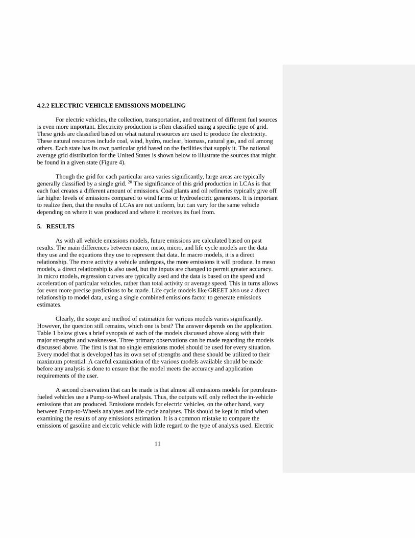
average grid distribution for the United States is shown below to illustrate the sources that might
be found in a given state (Figure 4).
Though the grid for each particular area varies significantly, large areas are typically
generally classified by a single grid. 20 The significance of this grid production in LCAs is that
each fuel creates a different amount of emissions. Coal plants and oil refineries typically give off
far higher levels of emissions compared to wind farms or hydroelectric generators. It is important
to realize then, that the results of LCAs are not uniform, but can vary for the same vehicle
depending on where it was produced and where it receives its fuel from.
5. RESULTS
As with all vehicle emissions models, future emissions are calculated based on past
results. The main differences between macro, meso, micro, and life cycle models are the data
they use and the equations they use to represent that data. In macro models, it is a direct
relationship. The more activity a vehicle undergoes, the more emissions it will produce. In meso
models, a direct relationship is also used, but the inputs are changed to permit greater accuracy.
In micro models, regression curves are typically used and the data is based on the speed and
acceleration of particular vehicles, rather than total activity or average speed. This in turns allows
for even more precise predictions to be made. Life cycle models like GREET also use a direct
relationship to model data, using a single combined emissions factor to generate emissions
estimates.
Clearly, the scope and method of estimation for various models varies significantly.
However, the question still remains, which one is best? The answer depends on the application.
Table 1 below gives a brief synopsis of each of the models discussed above along with their
major strengths and weaknesses. Three primary observations can be made regarding the models
discussed above. The first is that no single emissions model should be used for every situation.
Every model that is developed has its own set of strengths and these should be utilized to their
maximum potential. A careful examination of the various models available should be made
before any analysis is done to ensure that the model meets the accuracy and application
requirements of the user.
A second observation that can be made is that almost all emissions models for petroleum-
fueled vehicles use a Pump-to-Wheel analysis. Thus, the outputs will only reflect the in-vehicle
emissions that are produced. Emissions models for electric vehicles, on the other hand, vary
between Pump-to-Wheels analyses and life cycle analyses. This should be kept in mind when
examining the results of any emissions estimation. It is a common mistake to compare the
emissions of gasoline and electric vehicle with little regard to the type of analysis used. Electric

12
vehicles are often hailed by consumers and popular media as the perfect alternative to gasoline
powered vehicles. An uninformed user may tend to believe that electric vehicles produce almost
no in-vehicle emissions and compares this with normal, gasoline vehicles. In this comparison,
the user will find the electric car to be vastly superior. However, this type of analysis ignores a
major factor. The bulk of electric vehicle emissions are not produced during vehicle operation,
but rather during the production and assemblage of the vehicle, as well as the extraction and
processing of the vehicle’s fuel. If a user wants a true comparison between vehicle emissions, a
life cycle analysis must be done that takes into consideration all these factors. Though the results
may end up revealing that the electric car is still more efficient, the user will be surprised to find
that the improvement is not as drastic as it at first appeared. Also as mentioned previously, life
cycle analyses rarely take into account the disposal of materials. Especially in the case of electric
car batteries, the future consequences of large scale disposal are for the most part unknown.
Therefore, care must always be taken when comparing vehicle emissions. Whenever an
emissions analysis is done and the data set includes both gasoline and electric vehicles, it is
recommended that the GREET model be used for LCA or the MOVES and EMFAC models be
used for Pump-to-Wheels analysis so as to provide consistency between outputs.
A last observation is that as technologies continue to increase the performance and
functionality of vehicles, the need will arise to add another parameter to vehicle emissions
models. This parameter will need to take into account the technology used, much like the
EMFAC model has a “Technology Group” parameter. 12 This parameter will give reductions or
additions to the emissions based on the technology used. By the addition of this parameter,
developers will be able to rapidly adapt their models to incorporate new technologies.
6. CONCLUSIONS
This paper presented the most common technologies used to measure gasoline vehicle
emissions and how vehicle emission models rely on these measurements to model and estimate
vehicles emissions in real life conditions. The paper also presented a comparative synthesis
between the major gasoline and electric vehicle emission models, including: 1) Macro-scale
models: MOVES2014 and EMFAC; 2) Meso-scale models: VT-Meso, MOVES2014, and
MEASURE; 3) Micro-scale models: VT-Micro and CMEM; and 4) Electric and gasoline
lifecycle models: MOVES2014 and GREET. Furthermore, the paper highlighted common
misconceptions associated with comparing emission estimates resulting from models that are
based on different lifecycle stages, e.g. “well to wheel”, “tank- or pump- to-wheel”, or complete
lifecycle models.
The observations and summaries in this paper are meant to be used as a beneficial
introductory resource for researchers and users of vehicle emissions models. It is not
comprehensive and only introduces the main processes involved in the models described above.
This paper, however, presents an overview that would enable the reader to more easily
comprehend the differences between these models and determine the model that would be best
suited for a specific application. For a reader who is interested in learning about a specific model
in more detail, this paper provides reference to many other publications.

13
A possible extension of this work, which the authors are currently pursuing, involves the
simulation of a real-life network of intersections. This work would allow for a quantitative
comparison between the estimates of various models belonging to different network scales (i.e.
macro, meso, micro and LCA). This simulation takes into account both the scope and scale of the
model and could be used to test the relative speed and accuracy of the models when estimating
emissions.

14
7. WORKS CITED AND ADDITIONAL REFERENCES
1. Sources of Greenhouse Gas Emissions. U. S. Environmental Protection Agency, 2014.
2. The Southland's War on Smog: Fifty years of Progress Toward Clean Air. Southern
California Air Quality District, 2013.
3. On-Board Emissions Measurement System OBS-ONE Series. Horiba Automotive Test
Systems, 2012.
4. Standard Emissions. Horiba Automotive Test Systems, 2006.
5. Dynamometer Drive Schedule Quick View. U. S. Environmental Protection Agency,
2006.
6. Weiss, Martin, e. a., Analyzing on-road emissions of light-duty vehicles with Portable
Emission Measurement Systames (PEMS). JRC Scientific and Technical Reports, 2011.
7. Koupal, J. e. a., Draft Design and Implementation Plan for EPA's Multi-Scale Motor
Vehicle and Equipment Emission System (MOVES). U. S. Environmental Protection
Agency, 2002.
8. Frey, H. C.; Unal, Alper, Use of On-Board Tailpipe Emissions Measurements for
Development of Mobile Source Emission Factors.U. S. Environmental Protection
Agency, 2002.
9. Ahn, K., Dissertation on the development of the VT-Micro Model. TRB, 2002.
10. History of the Clean Air Act. U. S. Environmental Protection Agency, 2013.
11. Rakha, Hesham; Ahn, Kyoungho; Trani, Antonio, Comparison of MOBILE5A,
MOBILE6, VT-Micro, and CMEM Models for Estimating Hot-Stabilized Light-Duty
Gasoline Vehicle Emissions. Canadian Journal of Civil Engineering, 2003.
12. EMFAC2011 Technical Documentation. California Air Resources Board, 2011.
13. EMFAC2014 v0.3.6 User's Guide. California Air Resources Board, 2014.
14. Farnsworth, S., El Paso Comprehensive Modal Emissions Model (CMEM) Case Study.
Texas Transportation Institute, 2001.
15. Scora, G.; Barth, M., Comprehensive Modal Emissions Model (CMEM), Version 3.01 -
User's Guide. University of California, Riverside, Center for Environmental Research
and Technology, 2006.
16. Rakha, H.; Yue, H.; Dion, F., VT-Meso model framework for estimating hot-stabilized
light-duty vehicle fuel consuption and emission rates. Canadian Journal of Civil
Engineering, Vol. 38, 2011, p1274-1286.
17. Fomunung, I., e. a., Validation of the MEASURE Automodile Emissions Model: A
Statistical Analysis. Research and Innovative Technology Administration, Journal of
Transportation and Statistics, Vol. 3, 2001.
18. Motor Vehicle Emission Simulator - User Guide for MOVES2014. U. S. Environmental
Protection Agency, Assessment and Standards Division, 2014.
19. Life Cycle Thinking. World Steel Association, 2014.
20. GREET Life-Cycle Model. Argonne National Laboratory, Center for Transportation
Research, 2014.
21. Emissions from Hybrid and Plug-In Electric Vehicles. U. S. Department of Energy, 2014.

15
Figure 1: Simplified CMEM Model Process Flow Diagram 14
Figure 2: Synthetic drive cycle versus actual drive cycle for VT-Meso model (FWYF drive cycle)16
0
5
10
15
20
25
30
35
40
45
50
0 100 200 300 400 500
Spee
d (
mph)
Time (sec)
Synthetic Drive Cycle
Actual Drive Cycle

16
Figure 3: Life Cycle Analysis of Vehicles 19
Figure 4: National Average of Electric Grid Distribution of Fuel Sources for United States21
Electricity Sources
1
2
3
4
5
49.6% Coal
19.3% Nuclear
18.8% Gas
6.5% Hydro
3.0% Oil1.3% Biomass
0.6% Other Fossils
0.4% Wind
Others
Raw Material Acquisition/Procurement
Material
Processing
Vehicle
Assembly
Vehicle Service Life
Recycling
Disposal

17
Table 1: Summary of Vehicle Emissions Models
Emissions
Model Energy Source Scale
Significant Input
Parameters Strengths Weaknesses Best Use
MOVES
2014
Gasoline, Diesel, Compressed
Natural Gas
(CNG), Liquefied Petroleum Gas
(LPG), Ethanol (E-
85), Electric*
Macro,
Meso, Micro
Vehicle Miles Travelled,
Road Type, Age of Vehicle,
Speed Distribution, Meteorological Data, Vehicle
Type, Fuel Type
Uses extensive database from which it draws information;
Easy to use;
Can use as a framework for other location specific models, allowing users to specify
their own constants to be used when
calculating emissions factors; Includes emissions estimates for a wide
range of vehicle functions (e.g. hot soak,
tire wear, idling, etc.)
Poor for situations in which
there is highly variable
accelerations and decelerations; Do not include life cycle
analysis
Any "Pump-to-Wheels" analysis
EMFAC Gasoline, Diesel,
Electric* Macro
Fuel Type, Technology
Group, Model Year, Total
Activity, Population, Vehicle Miles Traveled, Trips
Generated per Day,
(See MOVES strengths above); Provides much more accurate emissions
estimates for California projects as
compared to the MOVES model
(See MOVES weaknesses above);
Model developed using data
specific to California
Any "Pump-to-Wheels" analysis in
California
VT-Meso Petroleum-Based Meso Average Vehicle Speed, Number of Stops made,
Stopped Delays
Requires very few input parameters;
Predicts HC, CO, and CO2 levels accurately;
Less data and time intensive than micro
emissions models
Is less accurate in situations
where there are large amounts of
speed variations or stop-and-go traffic
Projects in which a high level of accuracy is required, but the amount
of collected data is limited.
MEASURE Petroleum-Based Meso
Vehicle Registration Data, Travel-Demand Forecasts of
Flows, Speed and
Acceleration Distribution Tables, Socioeconomic Data
Works extremely well with GIS database
systems;
Can also be used to predict congestion levels and distributions of modal activities;
Statistical approach removes bias and can
result in more accurate emissions estimates
Statistical approach may cause
results to be vary slightly from
past data
Scenarios involving GIS databases
VT-Micro Petroleum-Based Micro Instantaneous Speed and
Acceleration of Vehicle
Accurately predicts emissions for highly variable speed and acceleration situations ;
Can be used with micro-simulation and
traffic signal optimization software
Cannot take into account vehicle operating conditions such as
deteriorated or malfuntioning
equipment
In conjunction with micro-simulation
software where the operating
conditions of the vehicles makes little differences and where a high level of
accuracy is required
CMEM Petroleum-Based Micro
Vehicle Speed and
Acceleration, Road Grade,
Engine Friction Factor, Cold Start Coefficients
Uses a physical, power-based approach
that takes into account different vehicle operating conditions;
Takes into account engine condition when
evaluating emissions
Predicts constant emissions for
deceleration events
In conjunction with micro-simulation
software where the operating conditions of the vehicles are a
concern and where a high level of
accuracy is required
GREET All Life-
Cycle
Fuel Source, Fuel Type, Fuel
Transportation Pathway, Fuel
Extraction and Vehicle Production Locations,
Vehicle Miles Travelled
Uses life cycle analysis to predict emissions;
Can evaluate a wide variety of vehicle
types and fuel pathways; Easy to use;
Best life cycle analysis currently available
for vehicle emissions analysis
Is less accurate in the prediction
of in-vehicle emissions;
Can only provide rough estimates of emissions related to
fuel extraction, transportation,
and refinement; Does not cover recycling or
disposal phases
Any "Well-to-Wheels" analysis
*Model estimates electric vehicle emissions using Pump-to-Wheels analysis only (See Section 4.2)