Understanding and Quantifying Motor Vehicle Emissions with VehicleSpecific Power and TILDAS Remote Sensing

by

José Luis Jiménez-Palacios

Double Mechanical Engineer Degree (1993)Universidad de Zaragoza (Spain)

Université de Technologie de Compiègne (France)

Submitted to the Department of Mechanical EngineeringIn Partial Fulfillment of the Requirements for the Degree of

Doctor of Philosophy in Mechanical Engineering

at the

Massachusetts Institute of Technology

February 1999

© 1999 Massachusetts Institute of TechnologyAll rights reserved

Signature of Author…………………………………………………………………………Department of Mechanical Engineering

December 5, 1998

Certified by…………………………………………………………………………………Gregory J. McRae

Bayer Professor of Chemical EngineeringThesis Supervisor

Accepted by………………………………………………………………………………...Ain A. Sonin

Mechanical Engineering Department Graduate Chair

Understanding and Quantifying Motor Vehicle Emissions with VehicleSpecific Power and TILDAS Remote Sensing

byJosé Luis Jiménez-Palacios

Submitted to the Department of Mechanical Engineeringon December 5, 1998 in partial fulfillment of the requirements

for the Degree of Doctor of Philosophy

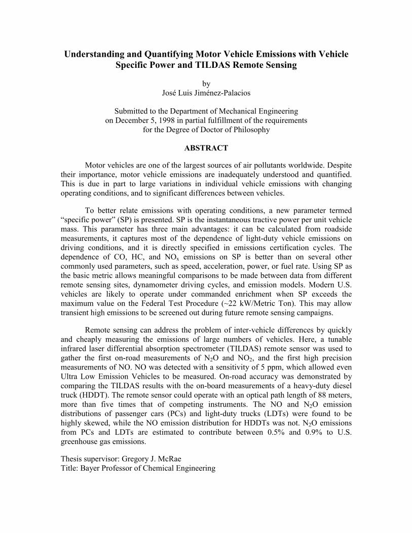
ABSTRACT

Motor vehicles are one of the largest sources of air pollutants worldwide. Despitetheir importance, motor vehicle emissions are inadequately understood and quantified.This is due in part to large variations in individual vehicle emissions with changingoperating conditions, and to significant differences between vehicles.

To better relate emissions with operating conditions, a new parameter termed“specific power” (SP) is presented. SP is the instantaneous tractive power per unit vehiclemass. This parameter has three main advantages: it can be calculated from roadsidemeasurements, it captures most of the dependence of light-duty vehicle emissions ondriving conditions, and it is directly specified in emissions certification cycles. Thedependence of CO, HC, and NOx emissions on SP is better than on several othercommonly used parameters, such as speed, acceleration, power, or fuel rate. Using SP asthe basic metric allows meaningful comparisons to be made between data from differentremote sensing sites, dynamometer driving cycles, and emission models. Modern U.S.vehicles are likely to operate under commanded enrichment when SP exceeds themaximum value on the Federal Test Procedure (~22 kW/Metric Ton). This may allowtransient high emissions to be screened out during future remote sensing campaigns.

Remote sensing can address the problem of inter-vehicle differences by quicklyand cheaply measuring the emissions of large numbers of vehicles. Here, a tunableinfrared laser differential absorption spectrometer (TILDAS) remote sensor was used togather the first on-road measurements of N2O and NO2, and the first high precisionmeasurements of NO. NO was detected with a sensitivity of 5 ppm, which allowed evenUltra Low Emission Vehicles to be measured. On-road accuracy was demonstrated bycomparing the TILDAS results with the on-board measurements of a heavy-duty dieseltruck (HDDT). The remote sensor could operate with an optical path length of 88 meters,more than five times that of competing instruments. The NO and N2O emissiondistributions of passenger cars (PCs) and light-duty trucks (LDTs) were found to behighly skewed, while the NO emission distribution for HDDTs was not. N2O emissionsfrom PCs and LDTs are estimated to contribute between 0.5% and 0.9% to U.S.greenhouse gas emissions.

Thesis supervisor: Gregory J. McRaeTitle: Bayer Professor of Chemical Engineering

AcknowledgmentsMy Ph.D. has been a multifaceted and enriching journey. I have profoundly changed, yet in

some ways I am still very much the same person who started this program. Five years of my life andlots of different people and experiences after, I am happy to see this journey finished. This is mychance to recognize those who contributed to make it possible.

First of all, I would like to thank my Ph.D. advisor, Greg McRae, for his support during mygraduate studies. He always had encouraging and positive things to say about my work, and was anendless source of suggestions. He also made me realize the importance of our field by circling theglobe 25 times while I was his grad student.

Next I would like to express my gratitude to Dave Nelson, Mark Zahniser, Barry McManus,and Chuck Kolb of Aerodyne Research, and to Michael Koplow of Emdot Corporation. Theyintroduced me to the TILDAS technique and were patient with my mistakes along the way. Workingwith them was one of the most rewarding experiences of these few years, and most importantly, wasalways fun.

I also want to thank my other thesis committee members, Bob Slott, John Heywood, andAhmed Ghoniem. Each one of them brought a very different perspective and working style whichmade for very enriching interactions. I also had many stimulating discussions about my thesis workwith Betty Pun, Ed Brown, Monika Mayer, Jochen Harnish, Frank Verdegem, Peter McClintock,Carlos Martinez, and Dave Kayes.

The many people of the McRae research group have provided a stimulating and fun workenvironment. I thank them for their companionship and all the fun moments spent together, and, lastbut not least, for their help with preparing my talks and especially my thesis defense. I will miss you! Ialso congratulate Liz Webb for managing the secretarial work with so much enthusiasm andefficiency.

I also spent one year of my Ph.D. working at the MIT Combustion Research Facility until itsclosure. I want to thank Janos Beer, Laszlo Barta, and the CRF research group for making that yearvery rich in learning and enjoyment.

César Dopazo of the University of Zaragoza helped me to come to MIT and generouslysupported me here for six months with his own group’s research funding, a gesture I have notforgotten and for which I want to express again my gratitude.

I also wish to acknowledge the South Coast Air Quality Management District for sponsoringa field measurement campaign; in-kind support from NASA and Hughes “Smog Dog;” help duringremote sensing campaigns from Steve Schmidt of Arthur D. Little, Nelson Sorbo of HughesEnvironmental Services, and Ed Brown, Foy King, and Bruce Harris of EPA; and financial supportfrom “La Caixa” Fellowship Program and from the EPA Office of Research and Development (grantnumber R824794-01-0).

I have been very lucky to have many friends in my years at MIT. To them I want to expressmy deepest gratitude for their humor, companionship, eagerness to follow when I suggested yetanother trip to explore the wild USA or another dance class, and also their support when research wasthin and my morale was low. You know who you are and I need not say more.

Finally I would like to thank my family. Their love (and illegal shipments of Spanish ham)has always been with me. I want to dedicate this thesis to them.

7 of 360

Table of Contents

Acknowledgments.............................................................................................................. 5

Table of Contents .............................................................................................................. 7

List of Figures .................................................................................................................. 13

List of Tables ................................................................................................................... 23

Nomenclature................................................................................................................... 25

Chapter 1. Introduction.................................................................................................. 291.1. Air Pollution ........................................................................................................... 291.2. The Contribution of Motor Vehicles to Air Pollution ............................................ 29

1.2.1. Capturing the Effect of Driving Conditions on Motor Vehicle Emissions 321.2.2. Quantifying Vehicle Emissions with High Precision Remote Sensing 331.2.3. Thesis Structure 341.2.4. Publications 35

Chapter 2. Background .................................................................................................. 372.1. Spectroscopic Basis of Remote Sensing................................................................. 37

2.1.1. Physical Basis for Remote Sensing: Beer’s Law 372.1.2. Molecular Absorption of Infrared Radiation 382.1.3. Absorption Lineshapes 402.1.4. Spectral Databases 412.1.5. Effect of Gas Temperature and Pressure on Molecular Absorption Lines 42

2.2. On-Road Remote Sensing....................................................................................... 432.2.1. Remote Sensing Setup 432.2.2. Principle of the Remote Sensing Measurement 432.2.3. Spectroscopic Techniques Used for On-Road Remote Sensing 442.2.4. Applications of Remote Sensing 48

2.3. Tunable Diode Lasers ............................................................................................. 502.3.1. Characteristics of Tunable Diode Lasers 502.3.2. Applications of TDLs to Atmospheric Measurements 51

Chapter 3. A New Definition of Specific Power and its Application to EmissionStudies .............................................................................................................................. 53

3.1. A New Definition of Specific Power ...................................................................... 543.1.1. Definition 543.1.2. Illustration of the Values of Specific Power for a Driving Cycle 573.1.3. Distribution of Specific Power in Driving Cycles and Remote Sensing Studies 593.1.4. Advantages of Specific Power for Emissions Studies 61

3.2. Analysis of Second-by-Second Emissions Data vs. Specific Power ...................... 663.2.1. Second-by-Second Emissions Data 663.2.2. Variations of the Emissions Results of Different Driving Cycles vs. SpecificPower 663.2.3. Specific Power vs. Speed and/or Acceleration 733.2.4. Use of Specific Power to Predict Commanded Enrichment Situations 75

8 of 360

3.2.5. Variation of the Emissions of Several Vehicles vs. Specific Power and OtherParameters 793.2.6. Effect of Payload Weight on Emissions 82

3.3. Applications of Specific Power for Remote Sensing............................................. 853.3.1. Transient High Emissions and Remote Sensing 853.3.2. Analogies Between Second-by-Second Driving Cycle Data and RemoteSensing Data 863.3.3. Criteria for Interpreting and Screening Remote Sensing EmissionMeasurements 873.3.4. Verification of Commanded Enrichment Screening Using Specific Power 883.3.5. False Failures Avoided by Specific Power Screening 893.3.6. Use of Specific Power to Compare Emissions Measured Under DifferentConditions 90

3.4. Applications of Specific Power for Emissions Modeling....................................... 983.4.1. Types of On-Road Vehicle Emissions Models 983.4.2. Use of Specific Power in Inventory Emissions Models 983.4.3. Use of Specific Power in Modal Emissions Modeling 100

3.5. Conclusions........................................................................................................... 102

Chapter 4. Analysis of Remote Sensing Measurements............................................. 1054.1. Introduction........................................................................................................... 1054.2. Fluid Mechanical Aspects of On-Road Remote Sensing...................................... 106

4.2.1. Automobile Wake Flow Patterns 1064.2.2. Geometry, Time-Scales, and Physical Effects for Automobile Remote Sensing 1084.2.3. Interference between the Exhaust of Two Vehicles 110

4.3. Variations in Plume Capture................................................................................. 1124.3.1. Parameters to Represent the Strength of Plume Capture 1124.3.2. Expected CO2 Column Density in Automobile Remote Sensing: FluidMechanical Model 1144.3.3. Expected CO2 Column Density in Automobile Remote Sensing: CylindricalExhaust Model 1154.3.4. Experimental Distribution of Plume Capture 1174.3.5. Variation of Plume Capture with Vehicle Speed, Acceleration, and SpecificPower for One Vehicle 1194.3.6. Variation of Plume Capture with Vehicle Speed, Acceleration, and SpecificPower for a Vehicle Fleet 1204.3.7. Plume Capture in the Heavy Duty Diesel Truck Measurements 122

4.4. Variations of the Precision of Remote Sensing Measurements ............................ 1244.5. Residence Time in the Exhaust System................................................................ 1294.6. Grams-per-mile vs. Grams per Gallon Emission Factors ..................................... 1344.7. The Need to Factor In Relative Fuel Economy .................................................... 1374.8. Conclusions of the Analysis of Remote Sensing Measurements.......................... 139

Chapter 5. The TILDAS Remote Sensor .................................................................... 1415.1. Introduction........................................................................................................... 1415.2. Optical layout of the instrument ........................................................................... 1425.3. Data Processing and Analysis Techniques ........................................................... 1445.4. Sensitivity and Accuracy of the TILDAS Remote Sensor.................................... 151

9 of 360

5.4.1. Estimation of the instrumental precision in the field 1515.4.2. Measurement of the NO Emissions from a Prototype Ultra Low EmissionsVehicle (ULEV) 1525.4.3. Accuracy of the NO Remote Sensor 153

5.5. Advantages of the TILDAS vs. NDIR Remote Sensing....................................... 1555.5.1. Frequency Resolution and Information Content 1555.5.2. Long Optical Path 156

5.6. Effects of Exhaust Temperature on TILDAS Remote Sensing Measurements.... 1595.6.1. Expected Gas Temperatures 1595.6.2. Effect of Temperature on the TILDAS Remote Sensing Measurements 160

5.7. Determination of Gas Temperature from TILDAS Remote Sensing Spectra ...... 1645.7.1. Motivation 1645.7.2. Previous Work on Gas Temperature Measurement using AbsorptionSpectroscopy 1645.7.3. Feasibility of Obtaining Temperature from TILDAS Remote Sensing Spectra 1665.7.4. Application of the Estimation Procedure to a Heavy-Duty Diesel Truck Plume 1675.7.5. Computational Strategy 169

5.8. Conclusions on TILDAS Remote Sensing ........................................................... 171

Chapter 6. Remote Sensing of NO Emissions from Automobiles and Light-DutyTrucks............................................................................................................................. 173

6.1. Introduction........................................................................................................... 1736.2. Experimental ......................................................................................................... 174

6.2.1. Experimental Site Description 1746.2.2. Likelihood of Vehicles in Cold Start Driving Through the Site 1746.2.3. Instrumentation 1766.2.4. Vehicle Speed and Acceleration Measurement 1786.2.5. License Plate Data Acquisition 1786.2.6. Decoding of Vehicle Information from the Vehicle Identification Numbers 1796.2.7. CO and HC Remote Sensing 181

6.3. Results of the Non-Emission Measurements ........................................................ 1826.3.1. Vehicle Statistics 1826.3.2. Distributions of Vehicle Age/Type and Emission Control Technologies 1836.3.3. Speed and Acceleration Distributions 1846.3.4. Specific Power Distribution 1856.3.5. Correlation Between Speed, Acceleration, and Specific Power in this Study 187

6.4. Results of NO Remote Sensing............................................................................. 1896.4.1. NO Emissions Distribution 1896.4.2. Why is the NO Emission Distribution so Skewed? 1926.4.3. Comparison to NOx Emission Factors and Ratios from Other Studies 1946.4.4. Correlation between Emissions and Vehicle Parameters 1956.4.5. Effect of Specific Power on NO Emissions: Individual Vehicles 1976.4.6. Effect of Specific Power on NO Emissions: Decile-Averaged Emissions 2016.4.7. Effect of Speed, and Acceleration on NO Emissions 2026.4.8. Correlation between NO Emissions and CO/HC Emissions 2056.4.9. Effect of Model Year on Emissions 2086.4.10. Comparison with the EMFAC model and Emission Standards 2106.4.11. Emission Contribution vs. Model Year 2136.4.12. NO Emissions Variability 213

10 of 360

6.4.13. High Emitters vs. Clean Vehicles 2146.4.14. NO Emissions and Vehicle Manufacturers: The Case of Honda 93-96 2186.4.15. Analysis of Failure Rates by Make for Arizona IM240 data 223

6.5. Conclusions of the NOx Remote Sensing Study................................................... 226

Chapter 7. Remote Sensing of NOx Emissions from Heavy-Duty Diesel Trucks .... 2297.1. Introduction........................................................................................................... 2297.2. Experimental ......................................................................................................... 231

7.2.1. Adaptation of the TILDAS technique for Application to Heavy-Duty DieselTrucks 2317.2.2. The EPA instrumented heavy-duty diesel truck 2337.2.3. Limitations Due to the Size of the Optical Equipment 234

7.3. Experimental Results ............................................................................................ 2367.3.1. Intercomparison of the NO/ CO2 Ratios from the EPA Truck and the TILDASRemote Sensor 2367.3.2. Measurement of the NO Emissions from Random Trucks on I-40 2377.3.3. Origin of the Shape of the Heavy-Duty Diesel Truck NOx EmissionDistribution 2407.3.4. Remote Sensing of the NO2/NO ratio 2427.3.5. Opacity Measurement 245

7.4. Estimation of the NOx Emission Factor for Heavy-Duty Diesel Trucks .............. 2487.4.1. Estimation of the NOx Emission Factor Based on the TILDAS Measurements 2487.4.2. Comparison to NOx Emission Factors from Other Studies 2487.4.3. Contributions to the NOx Inventory 250

7.5. Conclusions of this study...................................................................................... 251

Chapter 8. Remote Sensing of N2O Emissions from Automobiles and Light-DutyTrucks............................................................................................................................. 253

8.1. Introduction........................................................................................................... 2538.2. Evaluation of Remote Sensing for the Measurement of On-Road N2OEmissions ..................................................................................................................... 255

8.2.1. Cold start vs. Total N2O Emissions 2558.2.2. Variations on N2O Emissions for Different Driving Conditions 258

8.3. N2O Remote Sensing Results ............................................................................... 2618.3.1. Remote Sensing of N2O Emissions with TILDAS 2618.3.2. N2O Emissions Distribution 2618.3.3. Effect of Vehicle Type and Emission Control Technology on N2O Emissions 2658.3.4. Effect of Vehicle Model Year for TWC-equipped vehicles 2678.3.5. Fraction of Total Emissions Contributed by Every Model Year (TWC only) 2698.3.6. Characteristics of the N2O High Emitters 2718.3.7. Correlation of NO and N2O Emissions 2728.3.8. N2O to NO Ratio vs. Model Year 2738.3.9. Effect of Vehicle Specific Power on N2O Emissions 2748.3.10. Effect of Speed and Acceleration on N2O Emissions 2758.3.11. Correlation of N2O with CO and Hydrocarbon Emissions 2788.3.12. N2O Emission Variability 280

8.4. Further Analysis and Comparison to the Literature Studies................................. 2828.4.1. Interpretation of the N2O vs. NO Results 2828.4.2. Compilation of Literature Studies 284

11 of 360

8.4.3. Comparison of the Literature Studies 2888.4.4. Further Evidence of the Skewness of the N2O Distribution 288

8.5. N2O Emission Factors........................................................................................... 2928.5.1. N2O Emission Factor Estimation from TILDAS Remote Sensing Data 2928.5.2. Comparison to the Literature and IPCC / EPA N2O Emission Factors 2948.5.3. Mobile Source Contribution to the U.S. Greenhouse Gas Inventory 3018.5.4. Net Impact of Automotive Catalysts on the N2O Budget 303

8.6. Discussion............................................................................................................. 3058.6.1. Conclusions of the Experimental Results and the Analysis of the Literature 3058.6.2. N2O High Emitters 3068.6.3. Lowering Sulfur Gasoline for Reducing N2O Emissions 307

Chapter 9. Directions for Future Research ................................................................ 3099.1. Further Analysis of the Possibilities of Vehicle Specific Power .......................... 3099.2. Improved Quantification of Emissions from Mobile Sources .............................. 3119.3. N2O Emissions from Mobile Sources ................................................................... 3139.4. Quantification of Ammonia Emissions from Three-Way Catalyst EquippedVehicles........................................................................................................................ 3169.5. Further Development of the TILDAS Remote Sensor ......................................... 318

Chapter 10. Conclusions............................................................................................... 319

Appendix ........................................................................................................................ 329Appendix A. Units Used for Emission Factors............................................................ 329Appendix B. Scatter Plots of Second-by-Second Emissions vs. Specific Power fora Vehicle and 4 Driving Cycles ................................................................................... 332Appendix C. Determination of Improved Air Broadening Coefficients for someNO Absorption Lines................................................................................................... 336Appendix D. Correlation Between Emissions and Vehicle Parameters ...................... 337Appendix E. Correction of the N2O Automobile Measurement .................................. 338

E.1. Effect of Fringes on the N2O Emission Measurement 338E.2. Estimation of a Lower Bound of the Bias Size 339E.3. Average Correction of the Bias in the N2O Data Set 340

Appendix F. Characteristics of the Urban and Highway Test Cycles ......................... 343

References ............................................................................ Error! Bookmark not defined.

13 of 360

List of Figures

Chapter 1. Introduction.................................................................................................. 29Figure 1-1: California new passenger car emission standards....................................................... 30

Figure 1-2: Contribution of mobile sources to total U.S. emissions (U.S. EPA, 1997d)............... 30

Figure 1-3: Nonattainment areas for as of September 1997(from U.S. EPA, 1997c).................... 31

Chapter 2. Background .................................................................................................. 37Figure 2-1: Schematic of the transmission of a parallel beam through a gas ................................ 37

Figure 2-2: Schematic of 2 situations with more than one absorbing gas ..................................... 38

Figure 2-3: NO absorption bands around 1900 cm-1 showing individual absorption lines............ 39

Figure 2-4: Schematic of line shape and the fundamental spectroscopic parameters of a linetransition (the dotted line refers to a perturbed transition) (Rothman et al., 1998)......... 40

Figure 2-5: Spectral map showing the location of the absorption bands of the molecularspecies included in the 1996 HITRAN database (Rothman et al., 1998)........................ 41

Figure 2-6: Setup for on-road remote sensing of automobile emissions ....................................... 43

Figure 2-7: Schematic of the GM NDIR remote sensing instrument (Cadle et al., 1994)............. 45

Figure 2-8: NDIR bandpass filter and absorption bands of propane and water (Guenther et al.,1991) ............................................................................................................................... 46

Figure 2-9: Electron-Hole Combination Process Resulting in Laser Emission (Silfvast, 1996) ... 50

Chapter 3. A New Definition of Specific Power and its Application to EmissionStudies .............................................................................................................................. 53Figure 3-1: Values of the parameter (CD*A/m) for several passenger car classes and for light

duty trucks....................................................................................................................... 57

Figure 3-2: Speed vs. time trace for the US06 dynamometer test cycle........................................ 58

Figure 3-3: Values of the three components of the Specific Power vs. time during the US06cycle ................................................................................................................................ 58

Figure 3-4: Distributions of Specific Powers in 3 driving cycles and 2 remote sensing studies,and maximum rated Specific Powers of current production vehicles ............................. 59

Figure 3-5: Detail of the distributions of Specific Powers in 3 driving cycles and 2 remotesensing studies ................................................................................................................ 60

Figure 3-6: Distribution of Specific Powers in each bag of the FTP............................................. 60

Figure 3-7:Second-by-second engine-out (left) and tailpipe (right) CO, HC, and NOx

emissions vs. Specific Power for a 1994 Jeep Cherokee tested on the HL07 drivingcycle ................................................................................................................................ 67

Figure 3-8: Total carbon tailpipe emissions binned by Specific Power ranges for a 1994 JeepCherokee for 4 driving cycles ......................................................................................... 68

Figure 3-9: Engine-out CO emissions binned by Specific Power ranges for a 1994 JeepCherokee for 4 driving cycles ......................................................................................... 70

14 of 360

Figure 3-10: Tailpipe CO emissions binned by Specific Power ranges for a 1994 JeepCherokee for 4 driving cycles ......................................................................................... 71

Figure 3-11: Engine-out HC emissions binned by Specific Power ranges for a 1994 JeepCherokee for 4 driving cycles ......................................................................................... 71

Figure 3-12: Tailpipe HC emissions binned by Specific Power ranges for a 1994 JeepCherokee for 4 driving cycles ......................................................................................... 72

Figure 3-13: Engine-out NOx emissions binned by Specific Power ranges for a 1994 JeepCherokee for 4 driving cycles ......................................................................................... 72

Figure 3-14: Tailpipe NOx emissions binned by Specific Power ranges for a 1994 JeepCherokee for 4 driving cycles ......................................................................................... 73

Figure 3-15: Fuel flow into the engine as a function of acceleration and Specific Power for a1994 Jeep Cherokee tested on the FTP and HL07 driving cycles................................... 74

Figure 3-16: Second-by-second engine-out NOx emissions vs. acceleration and SpecificPower for a 1994 Jeep Cherokee tested on the FTP and HL07 driving cycles ............... 74

Figure 3-17: Contour plots of second-by-second engine-out NOx emissions for a 1993 JeepCherokee during the FTP cycle....................................................................................... 75

Figure 3-18: Percentage of the time at a given Specific Power level that the commandedenrichment strategy is used, for 6 vehicles tested on the HL07 cycle............................. 76

Figure 3-19: Percentage of the time at a given absolute power level that the commandedenrichment strategy is used, for 6 vehicles tested on the HL07 cycle............................. 77

Figure 3-20: Percentage of the time at a given percentage of the maximum engine power levelthat the commanded enrichment strategy is used, for 6 vehicles tested on the HL07cycle ................................................................................................................................ 77

Figure 3-21: Percentage of the seconds with commanded enrichment vs. relative accelerationand Specific Power.......................................................................................................... 78

Figure 3-22: Engine-out CO emissions binned by Specific Power ranges for 6 vehicles testedon the HL07 driving cycle .............................................................................................. 79

Figure 3-23: Engine-out CO emissions binned by absolute power ranges for 6 vehicles testedon the HL07 driving cycle .............................................................................................. 80

Figure 3-24: Engine-out CO emissions binned by fuel rate ranges for 6 vehicles tested on theHL07 driving cycle ......................................................................................................... 80

Figure 3-25: Engine-out CO emissions binned by fuel rate per unit vehicle weight ranges for6 vehicles tested on the HL07 driving cycle ................................................................... 81

Figure 3-26: Engine-out NOx emissions binned by Specific Power ranges for 6 vehicles testedon the HL07 driving cycle (left: vehicles w/o EGR; right: vehicles with EGR)............. 81

Figure 3-27: Engine-out NOx emissions binned by absolute power ranges for 6 vehicles testedon the HL07 driving cycle (left: vehicles w/o EGR; right: vehicles with EGR)............. 82

Figure 3-28: Engine-out and tailpipe CO emissions vs. Specific Power for a 1993 Ford 250with two different weights .............................................................................................. 83

Figure 3-29: Engine-out and tailpipe HC emissions vs. Specific Power for a 1993 Ford 250with two different weights .............................................................................................. 84

Figure 3-30: Engine-out and tailpipe NOx emissions vs. Specific Power for a 1993 Ford 250with two different weights .............................................................................................. 84

Figure 3-31: CO emission (measured by remote sensing) vs. Specific Power for a prototypeUltra Low Emissions Vehicle ......................................................................................... 89

15 of 360

Figure 3-32: CO emission (measured by remote sensing) vs. Specific Power for 540 remotesensing measurements..................................................................................................... 90

Figure 3-33: CO emissions vs. Specific Power for 2 remote sensing studies and engine-outand tailpipe second-by-second data for a vehicle on a driving cycle.............................. 91

Figure 3-34: NOx emissions vs. Specific Power for 2 remote sensing studies and engine-outand tailpipe second-by-second data for a vehicle on a driving cycle.............................. 92

Figure 3-35: HC emissions vs. Specific Power for 2 remote sensing studies and engine-outand tailpipe second-by-second data for a vehicle on a driving cycle.............................. 92

Figure 3-36: Schematic of the way to determine the emission distribution for new drivingconditions........................................................................................................................ 94

Figure 3-37: CO in the first measurement vs. the second measurement for the vehiclesmeasured twice in the Chicago data set (Popp et al., 1998a) .......................................... 95

Figure 3-38: Average CO in each 5% Specific Power bin for the first and the secondmeasurement for the vehicles measured twice in the Chicago data set (Popp et al.,1998a) ............................................................................................................................. 96

Figure 3-39: HC in each 5% Specific Power bin for the first and the second measurement forthe vehicles measured twice in the Chicago data set (Popp et al., 1998a) ...................... 96

Figure 3-40: NO in each 5% Specific Power bin for the first and the second measurement forthe vehicles measured twice in the Chicago data set (Popp et al., 1998a) ...................... 97

Figure 3-41: EMFAC speed correction factors vs. average cycle speed for the regulatedpollutants......................................................................................................................... 99

Chapter 4. Analysis of Remote Sensing Measurements............................................. 105Figure 4-1: Schematic representation of the flow patterns in the wake of an automobile

(Hucho, 1993) ............................................................................................................... 106

Figure 4-2: Flow patterns in the wake of 3 typical automobile rear-end shapes (Hucho, 1998) . 107

Figure 4-3: Computed speed vectors at a cross section normal to the vehicle velocity at ¼ carlengths behind the automobile (Johnson et al., 1996) ................................................... 107

Figure 4-4: Schematic of the important quantities for determination of flow time-scales .......... 109

Figure 4-5: Remote sensing spectra of NO showing the negative peaks due to interferencewith the exhaust of the previous vehicle ....................................................................... 111

Figure 4-6: Schematic of a remote sensing plume signal vs. time, with the definitions of theparameters used to describe plume capture................................................................... 113

Figure 4-7: Visualization of an axisymmetric jet showing the potential core and the jetbreakup and mixing region ........................................................................................... 114

Figure 4-8: Schematic diagram of the TDL laser beam traversing the exhaust jet...................... 115

Figure 4-9: Distribution of expected maximum CO2 column densities for the second-by-second data of a 1994 Jeep Cherokee tested on the FTP and HL07 driving cycles ...... 116

Figure 4-10: Variation of the expected maximum CO2 column densities vs. speed and specificpower for the second-by-second data of a 1994 Jeep Cherokee tested on the HL07driving cycle.................................................................................................................. 116

Figure 4-11: Scatter plot of the two plume capture parameters................................................... 117

Figure 4-12: Histogram of maximum CO2 column densities observed experimentally,compared to the results of the model in section 4.3.3 ................................................... 118

Figure 4-13: Histogram of integrated CO2 signal levels observed ............................................. 118

16 of 360

Figure 4-14: Effect of speed, acceleration, and specific power on the time-integrated CO2

signal for a single car measured repeatedly on the same location................................. 120

Figure 4-15: Effect of speed, acceleration, and specific power on the maximum CO2 signalfor a single car measured repeatedly on the same location ........................................... 120

Figure 4-16: Time-integrated CO2 signal vs. vehicle speed ........................................................ 121

Figure 4-17: Time-integrated CO2 signal vs. vehicle acceleration .............................................. 121

Figure 4-18: Time-integrated CO2 signal vs. vehicle specific power .......................................... 122

Figure 4-19: Time-integrated CO2 signal vs. specific power at a constant speed....................... 122

Figure 4-20: Histogram of maximum column densities observed on individual automobileand heavy-duty truck remote sensing measurements.................................................... 123

Figure 4-21: Effect of the noise in the NO and CO2 channels on the NO/CO2 ratiomeasurement ................................................................................................................. 125

Figure 4-22: Effect of Plume Overlap in the NO/CO2 Measurement Noise................................ 126

Figure 4-23: Average noise in the returned NO concentration (ppm) as a function of CO2

column density and NO emission level......................................................................... 126

Figure 4-24: Average noise in the returned NO concentration (% of NO concentration) as afunction of CO2 column density and NO emission level .............................................. 127

Figure 4-25: Location of the 1473 vehicles measured in California in the map of Figure 4-23.. 127

Figure 4-26: Distribution of residence times of the exhaust gases from the engine to thetailpipe, and of distance traveled during that period for a 1994 Jeep Cherokee duringthe FTP and HL07 driving cycles ................................................................................. 130

Figure 4-27: Distance traveled by a 1994 Jeep Cherokee while the exhaust gases move fromthe engine to the tailpipe vs. specific power (HL07 cycle) ........................................... 131

Figure 4-28: Distance traveled by a 1994 Jeep Cherokee while the exhaust gases move fromthe engine to the tailpipe vs. vehicle speed (FTP and HL07 cycles)............................. 132

Figure 4-29: Contour plot of the estimated distance traveled by a 1994 Jeep Cherokee whilethe exhaust travels from engine to tailpipe for (FTP and HL07 cycles) ....................... 132

Figure 4-30: Engine out emission rates of NOx (gpg and gpm) during the HL07 cycle for a1993 Toyota Corolla ..................................................................................................... 135

Figure 4-31: Distribution of engine out CO emissions during the HL07 driving cycle for a1993 Toyota Corolla ..................................................................................................... 136

Figure 4-32: Distribution of engine out NOx emissions during the HL07 driving cycle for a1993 Toyota Corolla ..................................................................................................... 136

Chapter 5. The TILDAS Remote Sensor .................................................................... 141Figure 5-1: Optical layout of the TILDAS dual laser instrument ................................................ 142

Figure 5-2: Sawtooth current input used to modulate the diode laser frequency......................... 145

Figure 5-3: Methane spectrum obtained with a TILDAS spectrometer....................................... 147

Figure 5-4: Two laser combined frequency scan......................................................................... 148

Figure 5-5: Column densities of NO, N2O and CO2 in the wake of a vehicle as a function oftime. .............................................................................................................................. 149

Figure 5-6: Regression analysis to determine NO and N2O emission indices............................. 150

Figure 5-7: NO emissions of the Ultra Low Emission Vehicle vs. time. .................................... 152

17 of 360

Figure 5-8: Comparison of the TILDAS and NDIR spectral views of the NO absorption linesaround 1900 cm-1........................................................................................................... 155

Figure 5-9: Setup of the TILDAS instrument with a very long pathlength ................................. 157

Figure 5-10: NO and CO2 vs. time in a measurement of the EPA instrumented truck acrossroad I-54........................................................................................................................ 158

Figure 5-11: NO vs.CO2 for each data point in time for a measurement of the EPAinstrumented truck across road I-54 .............................................................................. 158

Figure 5-12: Speed, engine-out temperature, and catalyst temperature for a 1994 JeepCherokee tested on the Federal Test Procedure ............................................................ 159

Figure 5-13: Exhaust temperature measured with a thermocouple at the tailpipe vs. vehiclespeed for a vehicle driven in the Boston area................................................................ 160

Figure 5-14: Effect of temperature on some CO2 and NO transitions ......................................... 161

Figure 5-15: NO and CO2 vs. time, and NO vs. CO2 for a remote sensing measurement .......... 161

Figure 5-16: Chi-square returned by the spectra fitting program vs. assumed temperature ........ 166

Figure 5-17: RMS error in the estimation of the gas temperature from NO spectra vs. NOcolumn density .............................................................................................................. 167

Figure 5-18: TILDAS estimate of temperature for the plume in Figure 5-15 and confidenceintervals for the noise based on Figure 5-17 ................................................................. 168

Figure 5-19: 95% confidence interval of the error in the estimation of temperature (K) fromremote sensing NO spectra, vs. NO emission level and plume capture........................ 168

Chapter 6. Remote Sensing of NO Emissions from Automobiles and Light-DutyTrucks............................................................................................................................. 173Figure 6-1: Location of the remote sensing site at El Segundo ................................................... 174

Figure 6-2: Characteristics of the Hughes Way remote sensing site at El Segundo.................... 175

Figure 6-3: Photograph of the experimental setup at El Segundo ............................................... 176

Figure 6-4: Field instrumentation arrangement ........................................................................... 177

Figure 6-5: Model year distributions of the remote sensing data and of the VMT estimates ofEMFAC......................................................................................................................... 183

Figure 6-6: Model year distribution of emission control technologies........................................ 184

Figure 6-7: Speed and acceleration distributions......................................................................... 185

Figure 6-8: Distribution of specific power of the vehicles in this study, compared to thedistribution of specific powers during the FTP, IM240, and US06 test cycles............. 187

Figure 6-9: Scatter plot and linear regression of vehicle specific power vs. vehicle speed........ 188

Figure 6-10: Scatter plot and linear regression of vehicle specific power vs. vehicleacceleration ................................................................................................................... 188

Figure 6-11: Experimental NO emissions distribution and the gamma distribution of the samemean and standard deviation......................................................................................... 190

Figure 6-12: Comparison of the frequency of NO emission readings from –50 to +50 ppm;and the convolution of a normal distribution of standard deviation 8 ppm with theexperimentally determined gamma distribution shown in Figure 6-11 ........................ 191

Figure 6-13: Decile plot of NO emissions in El Segundo. .......................................................... 192

18 of 360

Figure 6-14: Comparison of the distribution of engine out and tailpipe emissions during theFTP and HL07 cycles for a 1994 Jeep Cherokee with the remote sensing distributionmeasured in California .................................................................................................. 193

Figure 6-15: Comparison of the NOx emission factor for light-duty vehicles from this study tothose of several tunnel studies....................................................................................... 195

Figure 6-16: Scatter plot of NO emission vs. specific vehicle power.......................................... 197

Figure 6-17: Second-by-second engine-out NOx emission for a 1994 vehicle without EGRtested on 2 driving cycles.............................................................................................. 199

Figure 6-18: Second-by-second engine-out NOx emission for a vehicle with EGR tested on 2driving cycles ................................................................................................................ 199

Figure 6-19: Second-by-second tailpipe NOx emission for a 1994 vehicle tested on 2 drivingcycles............................................................................................................................. 200

Figure 6-20: Second-by-second tailpipe NOx emission for a 1994 vehicle with the lean-oncruise strategy in a driving cycle................................................................................... 200

Figure 6-21: NO remote sensing measurements for individual vehicles with superposedregions of most common emission values for 3 types of vehicles ................................ 201

Figure 6-22: Average NO emission vs. average vehicle specific power by population decile.... 202

Figure 6-23: Scatter plot and linear regression of NO emission vs. vehicle speed...................... 203

Figure 6-24: Average NO emission vs. average vehicle speed for every speed populationdecile ............................................................................................................................. 203

Figure 6-25: Scatter plot and linear regression of NO emission vs. vehicle acceleration. .......... 204

Figure 6-26: Average NO Emission and average vehicle acceleration for every accelerationpopulation decile. .......................................................................................................... 204

Figure 6-27: Scatter Plot and Linear Regression of NO Emission vs. CO Emission .................. 205

Figure 6-28: Average NO vs. CO emissions for vehicle population deciles ............................... 207

Figure 6-29: Scatter Plot and Regression of NO Emission vs. HC Emission.............................. 207

Figure 6-30: Average NO vs. HC emissions for vehicle population deciles ............................... 208

Figure 6-31: NO emission vs. vehicle age for the TILDAS remote sensing data........................ 209

Figure 6-32: Average NO (ppm) emissions versus vehicle model year ...................................... 209

Figure 6-33: Average NO (grams/mile) emissions versus vehicle model year ........................... 210

Figure 6-34: Average NO remote sensing emission vs. model year for passenger carscompared to the EMFAC model result and the emission standard of that model year . 211

Figure 6-35: Average NO remote sensing emission vs. model year for light-duty trucks,compared to the EMFAC model result and the emission standard of that model year . 212

Figure 6-36: Average NO, HC and CO emissions vs. model year .............................................. 212

Figure 6-37: Total NO, HC and CO emissions by model year .................................................... 213

Figure 6-38: NO emissions in the first and second passes vs. the average emissions forvehicles measured more than once................................................................................ 214

Figure 6-39: Contribution to the total emissions of CO, HC, and NO by different groups ofvehicles ......................................................................................................................... 215

Figure 6-40: Age distribution of several types of vehicles measured by remote sensing............ 217

Figure 6-41: NO emissions vs. model year for Honda and the rest of the manufacturers(passenger cars only)..................................................................................................... 218

19 of 360

Figure 6-42: Average engine displacement of passenger cars vs. model year for Honda andthe rest of the manufacturers ......................................................................................... 219

Figure 6-43: CO emissions vs. model year for Honda and the rest of the manufacturers(passenger cars only)..................................................................................................... 219

Figure 6-44: HC emissions vs. model year for Honda and the rest of the manufacturers(passenger cars only)..................................................................................................... 220

Figure 6-45: N2O emissions vs. model year for Honda and the rest of the manufacturers(passenger cars only)..................................................................................................... 220

Figure 6-46: Comparison of the average emissions for each pollutant for Honda vs. the rest ofthe manufacturers (passenger cars only) ....................................................................... 221

Figure 6-47: Comparison of the distribution of NO emissions between Honda and the rest ofthe manufacturers for model years 93-96...................................................................... 222

Figure 6-48: Arizona IM240 failure rates of 6 manufacturers relative to the fleet average for agiven model year........................................................................................................... 222

Figure 6-49: Failure rates by manufacturer in Arizona IM240 program for 1991 vehicles ........ 225

Chapter 7. Remote Sensing of NOx Emissions from Heavy-Duty Diesel Trucks .... 229Figure 7-1: Two heavy-duty truck tractors showing the location of the exhaust pipes ............... 231

Figure 7-2: Optical layout for the remote sensing of emissions from heavy-duty diesel trucks . 232

Figure 7-3: Setup of the continuous gas analyzers in the EPA instrumented trailer.................... 234

Figure 7-4: Layout of gas analyzers, calibration gas bottles, and load inside the EPAinstrumented trailer ....................................................................................................... 234

Figure 7-5: Comparison of the EPA and TILDAS NOx/CO2 measurement for themeasurements taken on June 16, 97.............................................................................. 236

Figure 7-6: Two video frames taken during an emission measurement on I-40.......................... 237

Figure 7-7: Comparison of the distribution of the NO/CO2 ratios in the emissions ofautomobiles and heavy-duty diesel trucks .................................................................... 239

Figure 7-8: Comparison of the distribution of the NO/CO2 ratios measured in this and anotherremote sensing study of heavy-duty trucks and the distribution of the second-by-second emissions from the EPA instrumented truck..................................................... 241

Figure 7-9: Simultaneous spectra of NO2 and NO from a 10-cm reference cell ......................... 242

Figure 7-10: Simultaneous NO2 and NO spectra recorded by remote sensing of the EPAinstrumented truck......................................................................................................... 243

Figure 7-11: Time domain and X-Y plot of a NO/ NO2 remote sensing measurement of theEPA truck...................................................................................................................... 243

Figure 7-12: Transmitted light vs. CO2 column density (i.e. plume capture) for ameasurement on the EPA instrumented truck ............................................................... 247

Figure 7-13: Comparison of the heavy-duty NOx emission factor obtained in this study andthose of other studies..................................................................................................... 249

Chapter 8. Remote Sensing of N2O Emissions from Automobiles and Light-DutyTrucks............................................................................................................................. 253Figure 8-1: N2O exhaust concentration vs. time during the FTP for 3 vehicles (from the data

of Barton and Simpson (Barton et al., 1994), .............................................................. 256

20 of 360

Figure 8-2: FTP-composite vs. FTP-bag 2 (hot stabilized) N2O Emission for 5 literaturestudies (log-scale) ......................................................................................................... 257

Figure 8-3: FTP-composite vs. FTP-bag 2 (hot stabilized) N2O Emission for 5 literaturestudies (linear scale)...................................................................................................... 257

Figure 8-4: HWFET cycle N2O emission vs. FTP composite emission for 4 literature studies .. 259

Figure 8-5: IM240 vs. FTP-composite N2O emissions for the study of Barton et al. (Barton etal., 1994) ....................................................................................................................... 260

Figure 8-6: Histogram of N2O emissions for the 1386 measurements taken at El Segundo ....... 262

Figure 8-7: Convolution of gamma and normal distributions vs. experimental N2Odistribution .................................................................................................................... 263

Figure 8-8: Theoretical gamma distribution of N2O emission and experimental distribution.... 264

Figure 8-9: Decile plot of the experimental N2O distribution and of the hypothesized gammadistribution .................................................................................................................... 265

Figure 8-10: Average N2O emission rate for each vehicle type / control technology group forthe remote sensing data (labels are the number of vehicles for each type), ................. 267

Figure 8-11: Average N2O emissions (ppm) vs. vehicle model year for vehicles subject topassenger car and light-duty truck standards (remote sensing data) ............................. 268

Figure 8-12: Average N2O emissions (mg/mi) vs. vehicle model year for vehicles subject topassenger car and light-duty truck standards (remote sensing data) ............................. 269

Figure 8-13: Total contribution of every model year to the fleet N2O emissions........................ 270

Figure 8-14: Comparison of the model year contribution to total emissions for NO and N2O ... 270

Figure 8-15: Fraction of high N2O emitters for every model year for TWC-equippedpassenger cars (left) and light-duty trucks (right) ......................................................... 272

Figure 8-16: Scatter Plot of NO Emission vs. N2O Emission...................................................... 272

Figure 8-17: Average N2O Emission for Vehicles of Different NO levels.................................. 273

Figure 8-18: Ratio of average N2O to average NO emission vs. model year (TWC-equippedvehicles only) ................................................................................................................ 274

Figure 8-19: Scatter Plot and Linear Regression of N2O Emission vs. Vehicle Specific Power. 275

Figure 8-20: Average N2O emission vs. average specific power for each specific powerpopulation decile. .......................................................................................................... 275

Figure 8-21: Scatter Plot and Linear Regression of N2O Emission vs. Vehicle Speed ............... 276

Figure 8-22: Average N2O emission and average vehicle speed for every speed populationdecile ............................................................................................................................. 277

Figure 8-23: Scatter plot and linear regression of N2O emission vs. vehicle acceleration .......... 277

Figure 8-24: Average N2O emission vs. average acceleration for every accelerationpopulation decile ........................................................................................................... 278

Figure 8-25: Scatter plot of N2O emission vs. CO emission. ...................................................... 279

Figure 8-26: Average N2O emission vs. average CO emission for each CO population decile .. 279

Figure 8-27: Scatter Plot of N2O Emission vs. HC Emission...................................................... 280

Figure 8-28: Plot of average N2O emission vs. average HC emission for each HC populationdecile ............................................................................................................................. 280

Figure 8-29: N2O emission on second pass versus N2O emission on first pass for vehiclesmeasured more than once.............................................................................................. 281

Figure 8-30: Mass-balance model of the formation of N2O in three-way catalyst ..................... 282

21 of 360

Figure 8-31: (Left): Experimental N2O/NO ratio vs. NO in the exhaust compared to the modelresults; (Right): detail of the same graph for low NO................................................... 283

Figure 8-32: Experimental N2O vs. NO trend compared to the model results ........................... 284

Figure 8-33: Comparison of the N2O emission rates for passenger cars equipped with agedthree-way catalysts........................................................................................................ 287

Figure 8-34: Distribution of the N2O emission rates reported in the literature and comparisonto a gamma distribution (aged-TWC cars only)............................................................ 290

Figure 8-35: Distribution of the N2O emission rates reported in the literature compared to theremote sensing distribution (aged-TWC cars only) ...................................................... 291

Figure 8-36:Effect of sulfur content of the fuel on N2O emissions from TWC-vehicles ............ 293

Figure 8-37: : Comparison of N2O emission levels for all vehicle and catalyst types (II) .......... 299

Figure 8-38: : Comparison of N2O emission factors all vehicle and catalyst types..................... 300

Figure 8-39: Comparison of the mobile source contribution to U.S. greenhouse gas emissionsfor different sets of emission factors ............................................................................. 302

Figure 8-40: Comparison of the contribution of the different vehicle / technology types tomobile source N2O in the U.S. using the remote sensing estimates (left) and theaverage of the literature (right) ..................................................................................... 302

Figure 8-41: Schematic budget of N2O emissions with and without automotive catalysts ......... 303

Appendix ........................................................................................................................ 329Figure B-1 (below): Second-by-second engine-out NOx, CO, and HC emissions vs. vehicle

specific power for a 1994 Jeep Cherokee tested twice in each of 4 driving cycles ...... 332

Figure B-2(below): Second-by-second tailpipe NOx, CO, and HC emissions vs. vehiclespecific power for a 1994 Jeep Cherokee tested twice in each of 4 driving cycles ...... 333

Figure E-1:CO2-N2O channel spectra from a car’s exhaust plume showing the baselinecurvature and the small negative N2O peak produced by the non-linear least squaresfitting............................................................................................................................. 338

Figure E-2: Average N2O vs. Average NO for the lowest 28 bins of 1% of the cars ranked byNO................................................................................................................................. 339

Figure E-3: N2O emissions reported in the literature for non-catalyst vehicles and IPCCestimates........................................................................................................................ 340

Figure E-4: N2O Emission for non-catalyst cars and estimate of the average bias on the N2Omeasurements................................................................................................................ 341

Figure F-1: Speed vs. time profile and main statistics of the FTP (urban) driving cycle ............ 343

Figure F-2: Speed vs. time profile and main statistics of the HFET (highway) driving cycle .. 343

23 of 360

List of Tables

Chapter 4. Analysis of Remote Sensing Measurements............................................. 105Table 4-1: Time scales relevant to remote sensing...................................................................... 109

Table 4-2: Statistics of the distributions of the parameters measuring plume capture ................ 117

Table 4-3: Statistics of the distributions of engine out CO and NOx emissions during theHL07 cycle for a 1993 Toyota Corolla ......................................................................... 135

Chapter 6. Remote Sensing of NO Emissions from Automobiles and Light-DutyTrucks............................................................................................................................. 173Table 6-1: Summary of the output parameters provided by the Radian VIN decoder for every

vehicle ........................................................................................................................... 180

Table 6-2: Vehicle statistics for the experimental campaign at El Segundo ............................... 182

Table 6-3: Summary of statistics of the speed and acceleration distributions ............................. 185

Table 6-4: Summary of statistics of the specific power distribution .......................................... 186

Table 6-5: Summary of Statistics of the NO Emissions Distribution .......................................... 189

Table 6-6: Statistically significant correlations (α=1%) between emissions and vehicleparameters ..................................................................................................................... 196

Table 6-7: Emission contribution of different categories of vehicles.......................................... 217

Table 6-8: Emissions difference and statistical significance (SS) for the different model yearsand pollutants ................................................................................................................ 221

Chapter 7. Remote Sensing of NOx Emissions from Heavy-Duty Diesel Trucks .... 229Table 7-1: Summary of statistics for the distributions of NO/CO2 ratios measured for heavy-

duty trucks and automobiles ......................................................................................... 238

Table 7-2: Percentage of NO emissions of the dirtiest 10% and cleanest 50% of the vehiclesfor the truck and automobile studies ............................................................................. 239

Table 7-3: Results of the NO2/NO measurements ....................................................................... 244

Table 7-4: TILDAS-derived emission factors for NO and NOx for heavy-duty diesel trucks..... 248

Table 7-5: Comparison of the heavy-duty NOx emission factor obtained in this study andthose of other studies..................................................................................................... 249

Table 7-6: Relative contributions of automobiles and heavy-duty trucks to the NOx inventorybased on the TILDAS emission factors ........................................................................ 250

Chapter 8. Remote Sensing of N2O Emissions from Automobiles and Light-DutyTrucks............................................................................................................................. 253Table 8-1: Summary of Statistics of the N2O Emissions Distribution......................................... 262

Table 8-2: Average Results of N2O Automobile Emission Measurements (mg / mi) ................ 285

Table 8-3: Literature studies used for the N2O emissions distribution of passenger cars withaged three-way catalysts ............................................................................................... 289

24 of 360

Table 8-4: Statistics of the N2O FTP literature tests of passenger cars with aged three-waycatalysts......................................................................................................................... 289

Table 8-5: Comparison of the high emitter statistics for the literature N2O and the TILDASN2O and NO distributions. ............................................................................................ 291

Table 8-6: Summary of the emission factors from previous studies and this study for eachvehicle and catalyst type ............................................................................................... 295

Appendix ........................................................................................................................ 329Table A-1: Moles of carbon per unit fuel for the most common transportation fuels ................. 330

Table C-1: Improved air broadening coefficients for the NO transitions used in this study ....... 336

Table D-1: Linear correlation coefficients between emission and vehicle variables. Grayedboxes indicates that the correlation is significant with α=1%. ..................................... 337

25 of 360

Nomenclature

A/C Air Conditioning

A/F Air-to-Fuel Ratio

ARB02 A dynamometer test cycle designed by the California Air Resources Board

CAA Clean Air Act

CAP Compliance Assurance Program

CARB California Air Resources Board

CH2O Formaldehyde

CO Carbon monoxide

CO2 Carbon Dioxide

DMV Department of Motor Vehicles

EGR Exhaust Gas Recirculation

EMFAC California’s emissions factor model

EPA U.S. Environmental Protection Agency

FIR Far Infrared

FTIR Fourier Transform Infrared Spectrometer

FTP Federal Test Procedure

FWHM Full Width at Half Maximum

GC Gas Chromatography

gpg Grams of pollutant emitted per gallon of fuel consumed

gpm Grams of pollutant emitted per mile traveled

GVW Gross Vehicle Weight

GVWR Gross Vehicle Weight Rating

HC Hydrocarbons

HDT Heavy-Duty Truck

HDDT Heavy-Duty Diesel Truck

HFET Highway Fuel Economy Test

HL07 Dynamometer driving cycle representing aggressive driving

HWFET See HFET

HWHM Half Width at Half Maximum

I/M Inspection and Maintenance Program

IM240 240-second driving cycle used in inspection and maintenance programs

IPCC Intergovernmental Panel on Climate Change

K Kelvin

kW Kilowatt

LDT Light-Duty Truck

LDV Light-Duty Vehicles

LEV Low-Emission Vehicle

MIR Mid Infrared

26 of 360

MMTCE Millions of Metric Tons of Carbon Equivalent

MOBILE EPA’s mobile source emissions model

NARSTO North American Research Strategy for Tropospheric Ozone

NDIR Non-Dispersive Infrared

NDUV Non-Dispersive Ultraviolet

NH3 Ammonia

NIR Near Infrared

NMHC Non-Methane Hydrocarbons

NMOG Non-Methane Organic Gases

N2O Nitrous oxide

NO Nitric oxide

NO2 Nitrogen dioxide

NOx Oxides of nitrogen (the sum of NO and NO2. N2O is not included).

OBD On-Board Diagnostics

OXY Oxidation Catalyst

PC Passenger Car

ppm Parts-per-million

ppmv Parts-per-million by volume

RS Remote Sensing

RSD Remote Sensing Device

SCAQMD South Coast Air Quality Management District

SCAQS South Coast Air Quality Study

SFTP Supplemental Federal Test Procedure

SI International system of units

SP Specific Power

SULEV Super Ultra Low Emission Vehicle

TCE Tons of Carbon Equivalent

TDL Tunable Diode Laser

TDLAS Tunable Diode Laser Absorption Spectroscopy

THC Total Hydrocarbons

Tier 0 A set of Federal emission standards for passenger cars and light-duty trucks

Tier 1 A set of Federal emission standards for passenger cars and light-duty trucks

Tier 2 A set of Federal emission standards for passenger cars and light-duty trucks

TILDAS Tunable Infrared Laser Differential Absorption Spectroscopy

TLEV Transitional Low-Emitting Vehicle

TWC Three-Way Catalyst

ULEV Ultra Low Emission Vehicle

US06 Regulatory driving cycle representing aggressive driving

UV Ultraviolet

VIN Vehicle Identification Number

VMT Vehicle-Miles Traveled

27 of 360

VOC Volatile Organic Compounds

VSP Vehicle Specific Power

WOT Wide Open Throttle

29 of 360

Chapter 1. Introduction

1.1. Air Pollution

Air pollution spans a wide range of spatial and temporal scales. Urban air quality

problems affect most large cities around the world (WHO/UNEP, 1992). Tropospheric

ozone in particular persists in the U.S. despite more than 30 years of regulation and

billions of dollars spent on emissions controls, although it is slowly improving as a result

of these efforts (U.S. EPA, 1998f). Air quality in many developing countries is

deteriorating (WHO/UNEP, 1992) because these countries generally lack the resources to

invest in emission controls.

Global air pollution problems have captured public attention, first because of

stratospheric ozone depletion, and more recently due to the debate about global warming.

In response to the latter concern, steps to stabilize and reduce the emissions of

greenhouse gases were agreed in the 1997 Kyoto protocol. If the predictions of

significant warming are confirmed, widespread changes in human activities will be

needed to fend off disastrous consequences.

1.2. The Contribution of Motor Vehicles to Air Pollution

Automobile-related air pollution did not attract much attention until about 1950.

Emissions from coal combustion and other uncontrolled industrial sources had been the

main sources of air pollution until then. The importance of automobiles was first

recognized in the Los Angeles area, where a new pollutant which irritated the eyes and

respiratory system was observed, mostly during the summer. Growing numbers of

gasoline-powered cars without any emission control system and the particular

meteorological conditions of the Los Angeles basin combined to produce a serious smog

problem that persists to this day. Automobile manufacturers first denied that cars were

the cause of the problem, but eventually the scientific evidence was too clear to be denied

(de Nevers, 1995).

The strategy chosen to deal with the problem was to impose limits on how much

pollution new cars could emit, the so-called “emission standards.” The first such

regulations were enacted in California in 1965 (Calvert et al., 1993). U.S. legislation

Chapter 1

30 of 360

followed in 1968. The early 1970s were marked by conflict between the U.S. EPA and

the automobile manufacturers because the emissions regulations were not achievable

using existing technology (de Nevers, 1995). The manufacturers did succeed in

developing the technology needed to meet these increasingly stricter regulations,

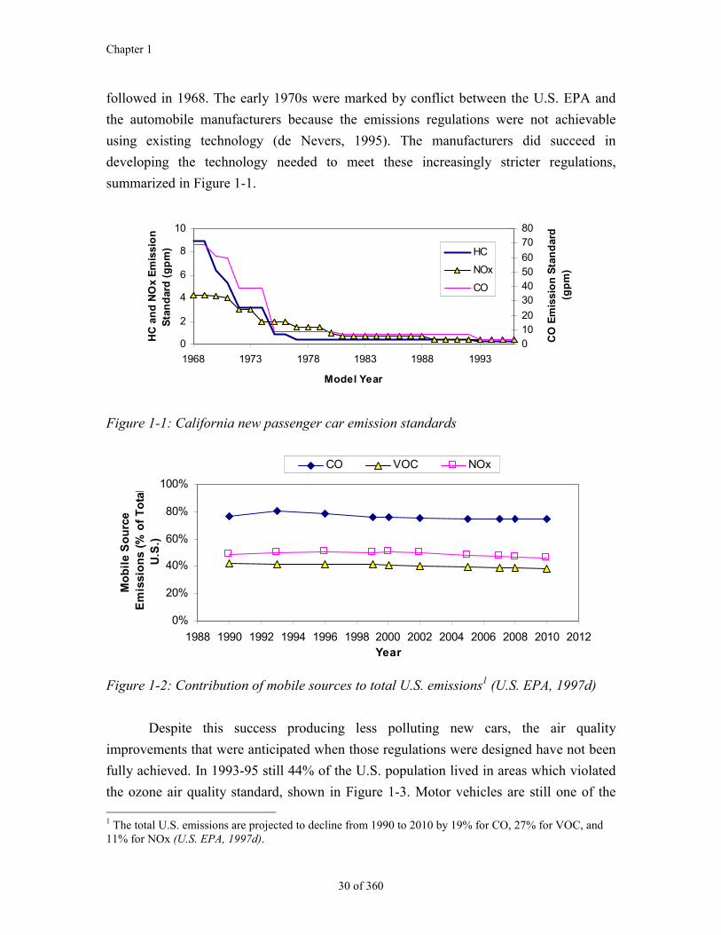
summarized in Figure 1-1.

0

2

4

6

8

10

1968 1973 1978 1983 1988 1993

Model Year

HC

an

d N

Ox

Em

issi

on

S

tan

dar

d (

gp

m)

01020

30405060

7080

CO

Em

issi

on

Sta

nd

ard

(g

pm

)

HC

NOx

CO

Figure 1-1: California new passenger car emission standards

0%

20%

40%

60%

80%

100%

1988 1990 1992 1994 1996 1998 2000 2002 2004 2006 2008 2010 2012Year

Mo

bil

e S

ou

rce

Em

issi

on

s (%

of

To

tal

U.S

.)

CO VOC NOx

Figure 1-2: Contribution of mobile sources to total U.S. emissions1 (U.S. EPA, 1997d)

Despite this success producing less polluting new cars, the air quality

improvements that were anticipated when those regulations were designed have not been

fully achieved. In 1993-95 still 44% of the U.S. population lived in areas which violated

the ozone air quality standard, shown in Figure 1-3. Motor vehicles are still one of the 1 The total U.S. emissions are projected to decline from 1990 to 2010 by 19% for CO, 27% for VOC, and11% for NOx (U.S. EPA, 1997d).

Introduction

31 of 360

largest sources of air pollutant emissions in the US, contributing 79% of the total CO,

42% of the VOC, 50% of the NOx, and 29% of the greenhouse gases in 1996 (U.S. EPA,

1996b; U.S. EPA, 1998c). This dominance is projected to continue in the future, as

illustrated by Figure 1-2.

Many U.S. States are finding it difficult to meet the current ozone and PM air

quality standards by the deadlines established in the Clean Air Act (U.S. EPA, 1997a).

For these reasons still stricter emission standards are being planned and implemented

(U.S. EPA, 1996a; U.S. EPA, 1997a; CARB, 1998c; U.S. EPA, 1998h), including a

“Super Ultra Low Emissions Vehicle” standard of 0.02 gpm NO (or a factor of 200

smaller than pre-control levels) in California (CARB, 1998c).

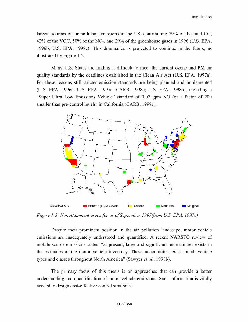
Figure 1-3: Nonattainment areas for as of September 1997(from U.S. EPA, 1997c)

Despite their prominent position in the air pollution landscape, motor vehicle

emissions are inadequately understood and quantified. A recent NARSTO review of

mobile source emissions states: “at present, large and significant uncertainties exists in

the estimates of the motor vehicle inventory. These uncertainties exist for all vehicle

types and classes throughout North America” (Sawyer et al., 1998b).

The primary focus of this thesis is on approaches that can provide a better

understanding and quantification of motor vehicle emissions. Such information is vitally

needed to design cost-effective control strategies.

Chapter 1

32 of 360

1.2.1. Capturing the Effect of Driving Conditions on Motor Vehicle Emissions

Many factors influence the emissions of a vehicle, including age, miles driven,

emission control technology, deterioration of the emission controls, tampering, ambient

temperature, and altitude. At present the emissions from the vehicle fleet are estimated by

models that attempt to account for many of those factors. Since these models are used by

air pollution control agencies in the design of new control strategies (U.S. EPA, 1993b;

CARB, 1998a), it is critical that the models reflect the true emissions as closely as

possible.

Unfortunately, significant problems exist. The SCAQS-1 Tunnel Study of 1987 in

the Los Angeles area “caused much consternation and head-scratching in the U.S. among

those involved in the development and use of mobile source emission factors”

(Halberstadt, 1990) by finding CO and HC emission rates that were higher than those

predicted by the models by factors of approximately 3 and 4, respectively (Pierson et al.,

1990). Subsequent studies have found that despite many improvements, emission models

still cannot consistently predict real-world emissions better than within about factor of 2,

although the size of the discrepancies has been reduced (Fujita et al., 1992; Kirchstetter et

al., 1996; Robinson et al., 1996; Singer and Harley, 1996; Dreher and Harley, 1998;

Gertler et al., 1998; Ipps and Popejoy, 1998).

Driving conditions strongly affect emissions but their effects are not well

quantified. As a result it is difficult to compare results based on different methods such as

instrumented vehicles, tunnel studies, remote sensing, dynamometer driving cycles, and

emissions modeling (or the results of different studies with the same method). A common

approach is to relate emissions to average speed (Carlson and Austin, 1997; CARB,

1998a). However, Webster and Shih (1996) showed that emissions could vary by an

order of magnitude for the same vehicle and average speed, due to small differences in

speed on a one-second time scale. Roadway grade is known to affect emissions (Cicero-

Fernandez and Long, 1995; Cicero-Fernandez and Long, 1996), but current inventory

models do not account for it (Beardsley, 1998; Long, 1998).

A large fraction of the emissions from light-duty vehicles and trucks comes from

a small fraction of the fleet with a malfunctioning control system (Stedman et al., 1994).

Inspection and Maintenance (I/M) programs are aimed at reducing these emissions.

Remote sensing can be used as a way to identify high emitters to be directed to inspection

and maintenance (I/M) facilities for testing, or to identify low emitters for exemption

Introduction

33 of 360

from I/M testing (“clean screening”). These actions can lead to more acceptable I/M

programs and more cost-effective improvements in air quality (Calvert et al., 1993;

Beaton et al., 1995). These applications, however, have been hampered by the variability

of vehicle emissions, such as the transient high emissions of properly operating vehicles.

These high emissions lead to false high emitter identification and have been one of the

main reasons why remote sensing has not been widely accepted for the detection of high

emitters (Lorang, 1998). A reliable method to screen out these occurrences is needed.

Chapter 3 of this thesis presents a new definition of specific power that captures

the dependence of emissions on driving conditions and is a good predictor of transient

high emissions. A very important property of this parameter is that it is measurable from

the roadside, and thus, it can be used by studies not having direct access to the vehicle

such as tunnel studies and remote sensing.

1.2.2. Quantifying Vehicle Emissions with High Precision Remote Sensing

Considerable effort has been expended to develop approaches to better quantify

motor vehicle emissions under actual operating conditions (Cadle et al., 1997; Cadle et

al., 1998). Tunnel studies (Pierson et al., 1990; Kirchstetter et al., 1996; Robinson et al.,

1996; Gertler et al., 1998) such as the SCAQS-1 mentioned above can be used to obtain

average fleet emission factors, while ambient air measurements in the vicinity of large

roadways (Fujita et al., 1992; Ipps et al., 1998) can assess the pollutant emission ratios

(CO/NOx and HC/NOx). However, neither of these methods can provide information

about vehicle-to-vehicle variations in emissions. Although it is possible to fit individual

vehicles with on-board instrumentation capable of pollutant monitoring, such

instrumentation is necessarily limited to a small number of test vehicles and cannot

measure the emissions of non-cooperative vehicles.

Remote sensing instruments using open path spectroscopy can measure the

emissions of thousands of vehicles per day. These measurements are made

simultaneously and immediately behind the moving vehicle and, thus, have the potential

to provide the best possible information on actual in-use vehicle emission profiles.

Remote sensing of CO and HC has been operational for a number of years.

Measurements of NO have lagged due to sensitivity problems. Current remote sensors

cannot reliably measure the emissions from very clean vehicles, nor can they quantify

other important species such as N2O or NH3.

Chapter 1

34 of 360

The range of current instruments is also very limited. Bishop and Stedman

(Bishop and Stedman, 1996c) report in a recent description of their NDIR-UV instrument

that “the system is designed to operate on a single lane road […] Multiple lane operation

has been reported but is not recommended.” A longer pathlength would allow greater

flexibility in the placement of the sensors. It would also diminish concerns of motorist

and operator safety which greatly limit site selection (Walsh and Gertler, 1997), of

vandalism of unmanned remote sensors, and of the suspected driving changes by drivers

aware of the presence of the remote sensor (Walsh et al., 1997).

Despite the more than 10 years since remote sensing was invented, some

important aspects of remote sensing measurements have not been quantified or

documented. Chapter 4 presents an analysis of a number of important issues which are

necessary for a proper interpretation of these measurements.

In Chapter 5 of this thesis, a high-precision, long-pathlength remote sensor is

presented. This instrument is based on Tunable Infrared Laser Differential Absorption

Spectroscopy (TILDAS), and has been developed to overcome some of the limitations of

existing remote sensors. It represents a major breakthrough with a sensitivity of 5 ppm of

the exhaust for NO, which allows the measurement of the emissions of even Ultra Low

Emission Vehicles. The measurement of minor species such as N2O, NO2, and NH3 is

also possible. A long path length capability has been demonstrated, which makes the

TILDAS technique particularly well suited for on and off-road vehicle emissions

measurements.

The TILDAS remote sensing instrument was used to answer some of the

outstanding questions about motor vehicle emissions. Chapters 6 and 8 contain the

analysis of the NO and N2O emissions of more than 1400 light duty vehicles and light

duty trucks. Chapter 7 presents the results of NO and NO2 remote sensing of heavy-duty

diesel trucks. A number of insights about the emission magnitudes, distributions,

correlations, and formation mechanisms have been obtained from an in-depth analysis of

these results.

1.2.3. Thesis Structure

This thesis is organized in the following manner:

Chapter 2 summarizes the relevant background.

Introduction

35 of 360

Chapter 3 introduces a new parameter, Specific Power, and shows its

usefulness for remote sensing and emissions modeling.

Chapter 4 analyzes some of the practical issues associated with remote

sensing measurements.

Chapter 5 presents the TILDAS technique and its application to remote

sensing.

Chapter 6 contains the analysis of a measurement campaign of NO emissions

from passenger cars and light-duty trucks.

Chapter 7 presents the analysis of the NO and NO2 emissions remotely sensed

from heavy-duty diesel trucks.

Chapter 8 is devoted to the analysis of the remote sensing measurements of

nitrous oxide (N2O) from cars and light-duty trucks.

Chapter 9 contains the directions for future research.

Chapter 10 presents the conclusions of this thesis.

1.2.4. Publications

Five conference papers have been presented on this work at the time of this

writing, and another one will be submitted to the 9th CRC workshop on vehicle

emissions. Part of chapter 5 has been published in Applied Physics B 62(4), 1998. Part of

chapter 6 has been accepted for publication in the Journal of Air and Waste Management

Association. Condensed versions of chapters 3 and 8 will be submitted to Environmental

Science and Technology. A version of chapter 7 will be submitted to the Journal of Air

and Waste Management Association.

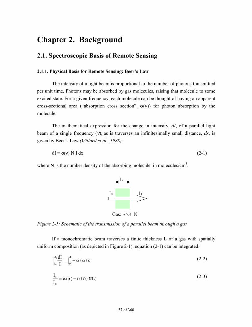
37 of 360

Chapter 2. Background

2.1. Spectroscopic Basis of Remote Sensing

2.1.1. Physical Basis for Remote Sensing: Beer’s Law

The intensity of a light beam is proportional to the number of photons transmitted

per unit time. Photons may be absorbed by gas molecules, raising that molecule to some

excited state. For a given frequency, each molecule can be thought of having an apparent

cross-sectional area (“absorption cross section”, σ(ν)) for photon absorption by the

molecule.

The mathematical expression for the change in intensity, dI, of a parallel light

beam of a single frequency (ν), as is traverses an infinitesimally small distance, dx, is

given by Beer’s Law (Willard et al., 1988):

dI = σ(ν) N I dx (2-1)

where N is the number density of the absorbing molecule, in molecules/cm3.

I0 I1

Gas: σ(ν), N

L

Figure 2-1: Schematic of the transmission of a parallel beam through a gas

If a monochromatic beam traverses a finite thickness L of a gas with spatially

uniform composition (as depicted in Figure 2-1), equation (2-1) can be integrated:

∫∫ −=L

0

I

Ió(õ)d

I

dI1

0

(2-2)

ó(õ)NL)(expI

I

0

1 −= (2-3)

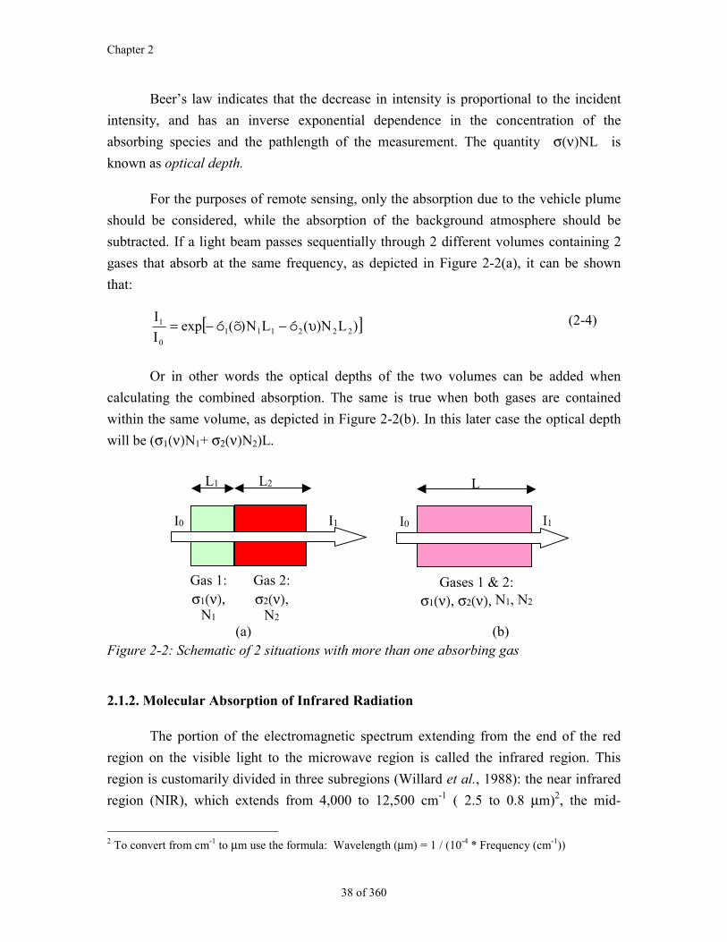
Chapter 2

38 of 360

Beer’s law indicates that the decrease in intensity is proportional to the incident

intensity, and has an inverse exponential dependence in the concentration of the

absorbing species and the pathlength of the measurement. The quantity σ(ν)NL is

known as optical depth.

For the purposes of remote sensing, only the absorption due to the vehicle plume

should be considered, while the absorption of the background atmosphere should be

subtracted. If a light beam passes sequentially through 2 different volumes containing 2

gases that absorb at the same frequency, as depicted in Figure 2-2(a), it can be shown

that:

[ ])L)N(óLN)(õóexpI

I222111

0

1 υ−−= (2-4)

Or in other words the optical depths of the two volumes can be added when

calculating the combined absorption. The same is true when both gases are contained

within the same volume, as depicted in Figure 2-2(b). In this later case the optical depth

will be (σ1(ν)N1+ σ2(ν)N2)L.

I0 I1

Gas 1:σ1(ν),

N1

L1

I0 I1

Gases 1 & 2:σ1(ν), σ2(ν), N1, N2

LL2

Gas 2:σ2(ν),

N2

I1

(a) (b)Figure 2-2: Schematic of 2 situations with more than one absorbing gas

2.1.2. Molecular Absorption of Infrared Radiation

The portion of the electromagnetic spectrum extending from the end of the red

region on the visible light to the microwave region is called the infrared region. This

region is customarily divided in three subregions (Willard et al., 1988): the near infrared

region (NIR), which extends from 4,000 to 12,500 cm-1 ( 2.5 to 0.8 µm)2, the mid-

2 To convert from cm-1 to µm use the formula: Wavelength (µm) = 1 / (10-4 * Frequency (cm-1))

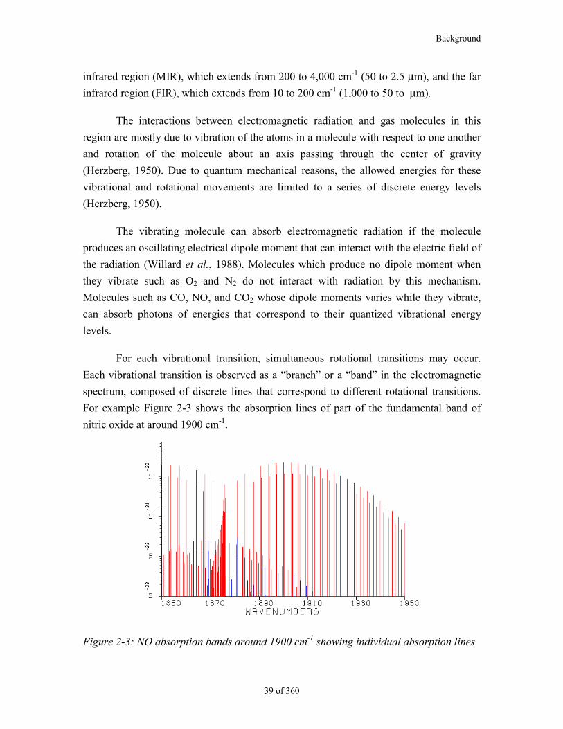
Background

39 of 360

infrared region (MIR), which extends from 200 to 4,000 cm-1 (50 to 2.5 µm), and the far

infrared region (FIR), which extends from 10 to 200 cm-1 (1,000 to 50 to µm).

The interactions between electromagnetic radiation and gas molecules in this

region are mostly due to vibration of the atoms in a molecule with respect to one another

and rotation of the molecule about an axis passing through the center of gravity

(Herzberg, 1950). Due to quantum mechanical reasons, the allowed energies for these

vibrational and rotational movements are limited to a series of discrete energy levels

(Herzberg, 1950).

The vibrating molecule can absorb electromagnetic radiation if the molecule

produces an oscillating electrical dipole moment that can interact with the electric field of

the radiation (Willard et al., 1988). Molecules which produce no dipole moment when

they vibrate such as O2 and N2 do not interact with radiation by this mechanism.

Molecules such as CO, NO, and CO2 whose dipole moments varies while they vibrate,

can absorb photons of energies that correspond to their quantized vibrational energy

levels.

For each vibrational transition, simultaneous rotational transitions may occur.

Each vibrational transition is observed as a “branch” or a “band” in the electromagnetic

spectrum, composed of discrete lines that correspond to different rotational transitions.

For example Figure 2-3 shows the absorption lines of part of the fundamental band of

nitric oxide at around 1900 cm-1.

Figure 2-3: NO absorption bands around 1900 cm-1 showing individual absorption lines

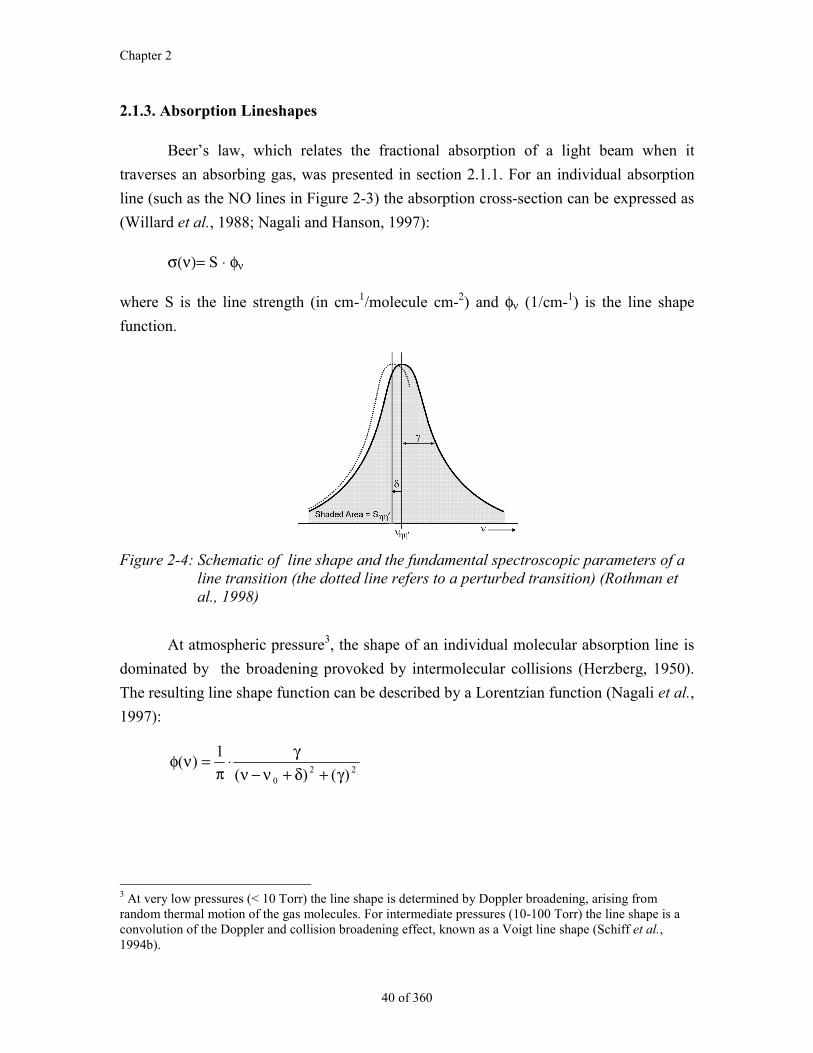
Chapter 2

40 of 360

2.1.3. Absorption Lineshapes

Beer’s law, which relates the fractional absorption of a light beam when it

traverses an absorbing gas, was presented in section 2.1.1. For an individual absorption

line (such as the NO lines in Figure 2-3) the absorption cross-section can be expressed as

(Willard et al., 1988; Nagali and Hanson, 1997):

σ(ν)= S ⋅ φν

where S is the line strength (in cm-1/molecule cm-2) and φν (1/cm-1) is the line shape

function.

Figure 2-4: Schematic of line shape and the fundamental spectroscopic parameters of aline transition (the dotted line refers to a perturbed transition) (Rothman etal., 1998)

At atmospheric pressure3, the shape of an individual molecular absorption line is

dominated by the broadening provoked by intermolecular collisions (Herzberg, 1950).

The resulting line shape function can be described by a Lorentzian function (Nagali et al.,

1997):

220 )()(

1)(

γ+δ+ν−νγ⋅

π=νφ

3 At very low pressures (< 10 Torr) the line shape is determined by Doppler broadening, arising fromrandom thermal motion of the gas molecules. For intermediate pressures (10-100 Torr) the line shape is aconvolution of the Doppler and collision broadening effect, known as a Voigt line shape (Schiff et al.,1994b).

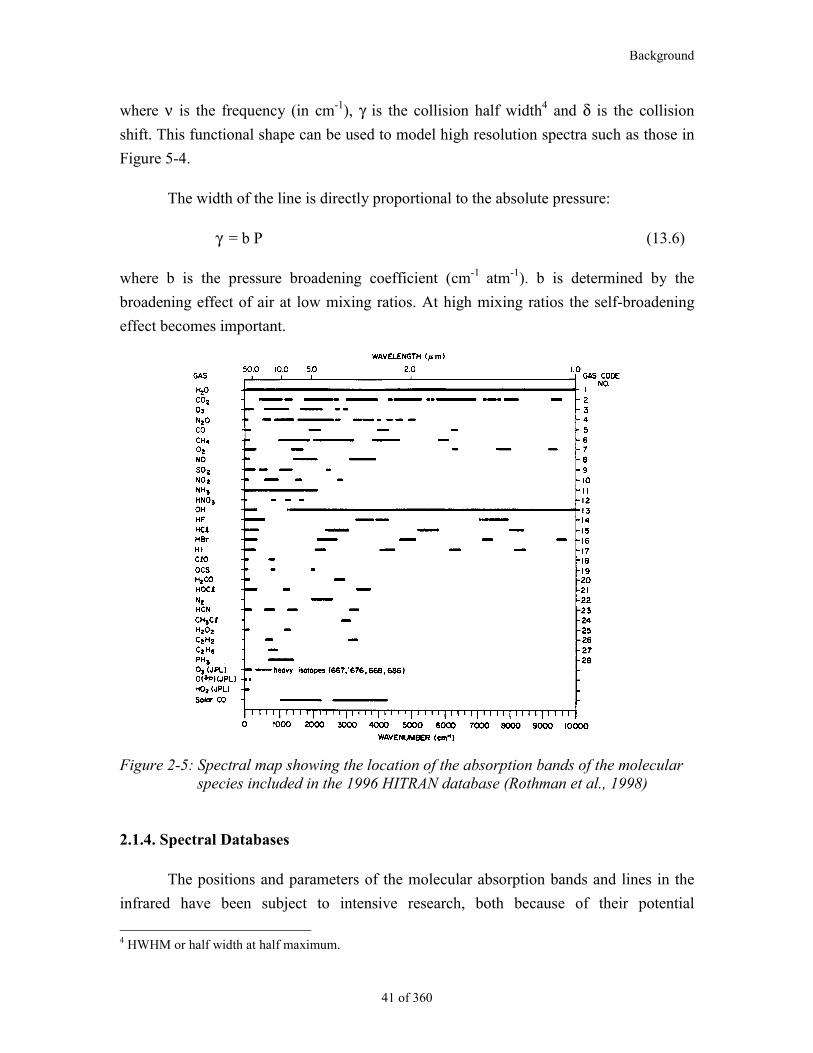
Background

41 of 360

where ν is the frequency (in cm-1), γ is the collision half width4 and δ is the collision

shift. This functional shape can be used to model high resolution spectra such as those in

Figure 5-4.

The width of the line is directly proportional to the absolute pressure:

γ = b P (13.6)

where b is the pressure broadening coefficient (cm-1 atm-1). b is determined by the

broadening effect of air at low mixing ratios. At high mixing ratios the self-broadening

effect becomes important.

Figure 2-5: Spectral map showing the location of the absorption bands of the molecularspecies included in the 1996 HITRAN database (Rothman et al., 1998)

2.1.4. Spectral Databases

The positions and parameters of the molecular absorption bands and lines in the

infrared have been subject to intensive research, both because of their potential

4 HWHM or half width at half maximum.

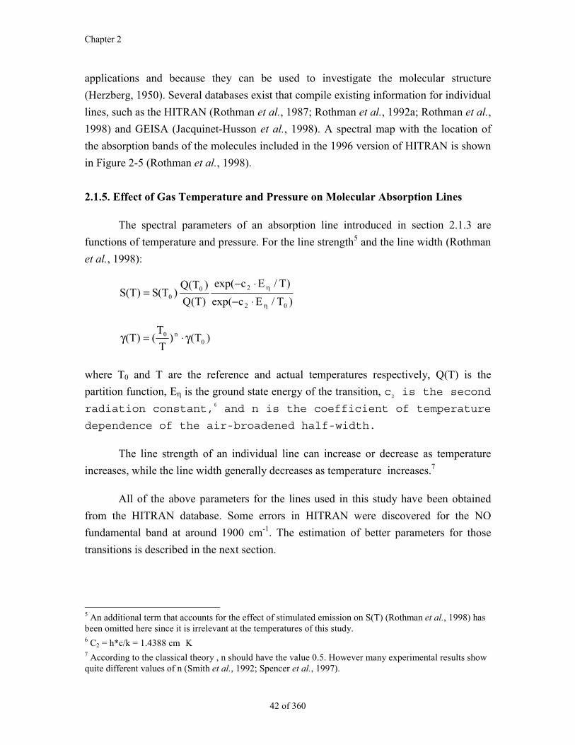
Chapter 2

42 of 360

applications and because they can be used to investigate the molecular structure

(Herzberg, 1950). Several databases exist that compile existing information for individual

lines, such as the HITRAN (Rothman et al., 1987; Rothman et al., 1992a; Rothman et al.,

1998) and GEISA (Jacquinet-Husson et al., 1998). A spectral map with the location of

the absorption bands of the molecules included in the 1996 version of HITRAN is shown

in Figure 2-5 (Rothman et al., 1998).

2.1.5. Effect of Gas Temperature and Pressure on Molecular Absorption Lines

The spectral parameters of an absorption line introduced in section 2.1.3 are

functions of temperature and pressure. For the line strength5 and the line width (Rothman

et al., 1998):

)T/Ecexp(

)T/Ecexp(

)T(Q

)T(Q)T(S)T(S

02

200

η

η

⋅−⋅−

=

)T()T

T()T( 0

n0 γ⋅=γ

where T0 and T are the reference and actual temperatures respectively, Q(T) is the

partition function, Eη is the ground state energy of the transition, c2 is the second

radiation constant,6 and n is the coefficient of temperature

dependence of the air-broadened half-width.

The line strength of an individual line can increase or decrease as temperature

increases, while the line width generally decreases as temperature increases.7

All of the above parameters for the lines used in this study have been obtained

from the HITRAN database. Some errors in HITRAN were discovered for the NO

fundamental band at around 1900 cm-1. The estimation of better parameters for those

transitions is described in the next section.

5 An additional term that accounts for the effect of stimulated emission on S(T) (Rothman et al., 1998) hasbeen omitted here since it is irrelevant at the temperatures of this study.6 C2 = h*c/k = 1.4388 cm K7 According to the classical theory , n should have the value 0.5. However many experimental results showquite different values of n (Smith et al., 1992; Spencer et al., 1997).

Background

43 of 360

2.2. On-Road Remote Sensing

2.2.1. Remote Sensing Setup

Cross-road remote sensing of vehicle emissions was pioneered by Don Stedman

and Gary Bishop of the University of Denver in 1987 (Bishop et al., 1989). The basic

idea is to use the fact that the different exhaust gases absorb light at different frequencies

to try to quantify them. The setup is illustrated in Figure 2-6. A light source(s) which

contains at least 2 different frequency regions is shined across the road to a detector.

When a vehicle goes by, its exhaust gases traverse the optical path of the laser light

causing some absorption which is detected and recorded. The analysis of the relative

absorption permits the quantification of a ratio of 2 gases, such as NO/CO2, which is the

primary result of the technique. From this ratio emission factors can be calculated as

detailed in Appendix A.

Retro-Reflector

Light Sourceand Detector

ExhaustPlume

VideoCamera

Data Acquisitionand Display

Light-PlumeOverlap

Figure 2-6: Setup for on-road remote sensing of automobile emissions

2.2.2. Principle of the Remote Sensing Measurement

The use of CO2 as a reference gas allows one to make quantitative measurements

of exhaust species without knowledge of the exhaust plume location or extent of dilution.

Exhaust water vapor could also be used in principle for this purpose, but its much larger

atmospheric background as compared to CO2 make it impractical.

Since all gases in the exhaust plume are transported together by turbulent

diffusion, the ratio of the measured column densities of NO and CO2 provides an

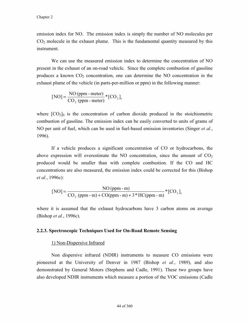
Chapter 2

44 of 360

emission index for NO. The emission index is simply the number of NO molecules per

CO2 molecule in the exhaust plume. This is the fundamental quantity measured by this

instrument.

We can use the measured emission index to determine the concentration of NO

present in the exhaust of an on-road vehicle. Since the complete combustion of gasoline

produces a known CO2 concentration, one can determine the NO concentration in the

exhaust plume of the vehicle (in parts-per-million or ppm) in the following manner:

s22

]CO[*meter)-(ppm CO

meter)-(ppm NO]NO[ =

where [CO2]S is the concentration of carbon dioxide produced in the stoichiometric

combustion of gasoline. The emission index can be easily converted to units of grams of

NO per unit of fuel, which can be used in fuel-based emission inventories (Singer et al.,

1996).

If a vehicle produces a significant concentration of CO or hydrocarbons, the

above expression will overestimate the NO concentration, since the amount of CO2

produced would be smaller than with complete combustion. If the CO and HC

concentrations are also measured, the emission index could be corrected for this (Bishop

et al., 1996c):

s22

]CO[*m)-HC(ppm*3m)-CO(ppmm)-(ppm CO

m)-(ppm NO]NO[

++=

where it is assumed that the exhaust hydrocarbons have 3 carbon atoms on average

(Bishop et al., 1996c).

2.2.3. Spectroscopic Techniques Used for On-Road Remote Sensing

1) Non-Dispersive Infrared

Non dispersive infrared (NDIR) instruments to measure CO emissions were

pioneered at the University of Denver in 1987 (Bishop et al., 1989), and also

demonstrated by General Motors (Stephens and Cadle, 1991). These two groups have

also developed NDIR instruments which measure a portion of the VOC emissions (Cadle

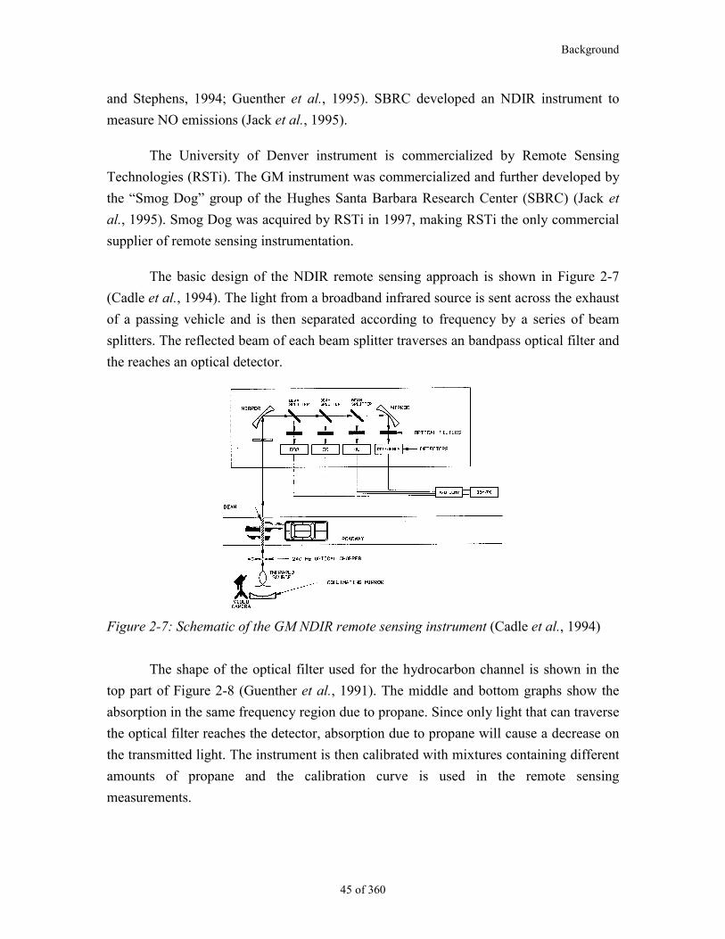
Background

45 of 360

and Stephens, 1994; Guenther et al., 1995). SBRC developed an NDIR instrument to

measure NO emissions (Jack et al., 1995).

The University of Denver instrument is commercialized by Remote Sensing

Technologies (RSTi). The GM instrument was commercialized and further developed by

the “Smog Dog” group of the Hughes Santa Barbara Research Center (SBRC) (Jack et

al., 1995). Smog Dog was acquired by RSTi in 1997, making RSTi the only commercial

supplier of remote sensing instrumentation.

The basic design of the NDIR remote sensing approach is shown in Figure 2-7

(Cadle et al., 1994). The light from a broadband infrared source is sent across the exhaust

of a passing vehicle and is then separated according to frequency by a series of beam

splitters. The reflected beam of each beam splitter traverses an bandpass optical filter and

the reaches an optical detector.

Figure 2-7: Schematic of the GM NDIR remote sensing instrument (Cadle et al., 1994)

The shape of the optical filter used for the hydrocarbon channel is shown in the

top part of Figure 2-8 (Guenther et al., 1991). The middle and bottom graphs show the

absorption in the same frequency region due to propane. Since only light that can traverse

the optical filter reaches the detector, absorption due to propane will cause a decrease on

the transmitted light. The instrument is then calibrated with mixtures containing different

amounts of propane and the calibration curve is used in the remote sensing

measurements.

Chapter 2

46 of 360

The main problem with this approach are interferences from other absorbing

gases. The filters used are very broad compared with individual absorption features (e.g.

more than 100 cm-1 in the one shown in Figure 2-8, compared with 0.25 cm-1 for a typical

absorption line at atmospheric pressure). Thus the likelihood of other species absorbing

in the same region as the filter is very large. For example the graph in the bottom of

Figure 2-8 shows absorption due to water vapor in the exhaust in the same region used

for hydrocarbon measurement. A possible solution is to try to measure the interfering

species at a different frequency and correct the measurement, e.g. the Hughes NO

instrument measures NO absorption in the infrared and corrects the measurement for

water vapor interferences (Jack et al., 1995).

Figure 2-8: NDIR bandpass filter and absorption bands of propane and water (Guentheret al., 1991)

2) Ultraviolet Absorption

UV absorption instruments have been developed to overcome the problem with

water vapor interference in the NDIR measurement of NO. The University of Denver

group developed an instrument based on this principle (Zhang et al., 1996a) for which it

claimed a precision (1σ) of about 300 ppm NO in the exhaust of the vehicle. Sjödin et al.

Background

47 of 360

(1996) attempted the development of a similar instrument based on UV DOAS which

claimed a similar precision.

Since most vehicles are thought to emit less than 300 ppm NO, a more sensitive

instrument was needed. The University of Denver group has developed a new ultraviolet-

based remote sensor with a standard deviation of about 20 ppm NO in the exhaust under

parking lot conditions (Popp et al., 1997). On-road data obtained with this instrument

have recently been presented (Popp et al., 1998a).

3) Near Infrared Tunable Diode Lasers

Schiff et al. (1994a) reported on the development of a near-infrared tunable diode

laser system for remote sensing.8 These researchers sensed the CO/CO2 ratios of a vehicle

running on a dynamometer, and also measured H2O and CH4 emissions. The detection

limits reported are on the range of 5-50 ppm-m (depending on the species).

Since a TILDAS column density detection limit of 0.1 ppm (10 Hz) for NO

translates into a sensitivity of about 3 ppm of the exhaust when measuring real cars, I

estimate that NIR TDLs could achieve sensitivities on the order of 150-1500 ppm of the

vehicle exhaust, which is comparable to what has been achieved using NDIR and UV

techniques.9,10 An attempt to extend this approach to NO emissions was impeded by the

lack of an adequate diode laser (Slott, 1997).

4) Gas-Filter Correlation

A gas-filter correlation (GFCR) instrument is in the early stages of development

(Sachse, 1998). The GFCR technique has been developed for satellite-based remote

sensing of atmospheric gases. This instrument will have the capability of measuring CO

and NO (using GFCR) and HCs (using the standard NDIR technique). The potential

sensitivity of the system is estimated at 10 ppm of the exhaust for CO and NO.

8 This instrument is described in more detail in a later publication (Schiff et al., 1996).9 This estimate assumes that the signal-to-noise ratio would be the same for the NIR TDL measurements asfor the TILDAS measurements. Some differences may exist owing to differences in laser diode poweroutput, detector response and noise, interferences, etc.10 Near infrared diode lasers at longer wavelengths have become available since the time of this study,allowing the use of stronger absorption transitions for some molecules (Allen, 1998). Thus the presentlyachievable sensitivities using this technique may be lower than these numbers.

Chapter 2

48 of 360

2.2.4. Applications of Remote Sensing

The ability to measure instantaneous on-road vehicle emissions by remote sensing

has many potential applications. Dozens of studies have been carried out to evaluate and

implement some of them. The most important applications proposed or accomplished to

date are:

High emitter detection for immediate pullover or direction to inspection and

maintenance programs (Bishop et al., 1993; Bishop et al., 1996c; Sjödin et al., 1996;

Sorbo et al., 1997)

Low emitter detection for exemption from inspection and maintenance programs

(Sjödin et al., 1996; Baker et al., 1997; Kishan et al., 1998; St. Denis, 1998; Wenzel

and Sawyer, 1998a)

Pre-screening of vehicles in inspection and maintenance facilities (Petherick, 1996;

Petherick, 1997).

Public information systems that display the emission status of cars as they drive by

(Bishop et al., 1996a).

Measurements at toll booths to charge higher tolls for gross polluters (Bishop et al.,

1996c).

Measurements of employees for employer-paid repairs (Bishop et al., 1996c).

Fleet Characterization (Zhang et al., 1993; Stedman et al., 1994; Zhang et al., 1994;

Zhang et al., 1995; Zhang et al., 1996a; Bishop et al., 1997; Stedman et al., 1997a;

Popp et al., 1998a)

Compilation of emissions inventories (Singer et al., 1996; Dreher et al., 1998).

Evaluation of inspection and maintenance programs or the impact or other emission

reduction programs such as reformulated fuels (Sjödin et al., 1997a; Stedman et al.,

1997b; Stedman et al., 1998)

Evaluation of the rates of deterioration and technological improvement of the

emission control systems (Slott, 1996).

Background

49 of 360

Detection of specific vehicle models with poor emission performance (Sjödin et al.,

1996; Wenzel and Ross, 1996; Wenzel and Ross, 1997; Wenzel et al., 1998b).

Comparing the emissions of vehicles with different technologies and/or fuels (Sjödin

et al., 1996; Riveros et al., 1998; Stedman et al., 1997a; Mercer and McArragher,

1997).

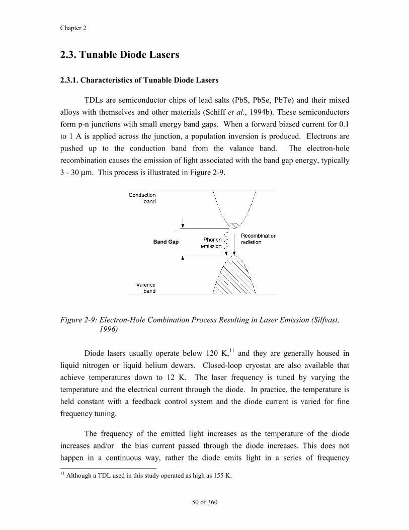
Chapter 2

50 of 360

2.3. Tunable Diode Lasers

2.3.1. Characteristics of Tunable Diode Lasers

TDLs are semiconductor chips of lead salts (PbS, PbSe, PbTe) and their mixed

alloys with themselves and other materials (Schiff et al., 1994b). These semiconductors

form p-n junctions with small energy band gaps. When a forward biased current for 0.1

to 1 A is applied across the junction, a population inversion is produced. Electrons are

pushed up to the conduction band from the valance band. The electron-hole

recombination causes the emission of light associated with the band gap energy, typically

3 - 30 µm. This process is illustrated in Figure 2-9.

Band Gap

Figure 2-9: Electron-Hole Combination Process Resulting in Laser Emission (Silfvast,1996)

Diode lasers usually operate below 120 K,11 and they are generally housed in

liquid nitrogen or liquid helium dewars. Closed-loop cryostat are also available that

achieve temperatures down to 12 K. The laser frequency is tuned by varying the

temperature and the electrical current through the diode. In practice, the temperature is

held constant with a feedback control system and the diode current is varied for fine

frequency tuning.

The frequency of the emitted light increases as the temperature of the diode

increases and/or the bias current passed through the diode increases. This does not

happen in a continuous way, rather the diode emits light in a series of frequency 11 Although a TDL used in this study operated as high as 155 K.

Background

51 of 360

“modes,” or frequency intervals where the diodes are continuously tunable. These modes

are separated by “mode breaks”, frequency intervals in which the diode does not emit any

light. One of the biggest drawbacks of tunable diode lasers is the instability of modes.

The frequency of the light emitted at a given temperature/current combination drifts with

time. If the laser is warmed up to room temperature mode structures may change

significantly, and some previously used absorption lines may no longer be within the

lasing region. The presence of mode breaks and mode instability makes selecting and

operating the tunable diode lasers a time consuming task.

2.3.2. Applications of TDLs to Atmospheric Measurements

Typical line widths of individual absorption lines at atmospheric pressure are on

the order of 0.05 cm-1. An adequate measurement of an individual line requires an

spectral resolution of about 0.005 cm-1 (10 points per line). Non-dispersive Infrared

(NDIR) and Fourier Transform Infrared (FTIR) spectrometers use broad band light

sources and are generally incapable of such resolution.

TDLs have line widths of the order of 0.001 cm-1 or smaller (Schiff et al., 1994b)

and are tunable in frequency. They can be used to scan over an individual absorption line,

the main requirement being that the molecule should have an infrared line spectrum

which is resolvable. This includes most molecules with up to 5 atoms and some larger

molecules (Werle, 1998).

The application of tunable diode lasers to atmospheric measurements is known as

TDL spectroscopy, Tunable Diode Laser Absorption Spectroscopy (TDLAS), and

Tunable Infrared Laser Differential Absorption Spectroscopy (TILDAS). The first and

third names are used indistinctly in this thesis.

Atmospheric trace gas measurements with tunable diode laser spectroscopy

generally use reduced pressure sampling to take advantage of the much narrower

absorption lines under these conditions. This technique is less frequently used in open

path remote sensing applications (Kolb et al., 1995) although the first applications of

TDLs to atmospheric measurements were open path measurements of ambient CO in

cities (Hinkley and Kelley, 1971; Ku et al., 1975).

The TILDAS technique has been used to measure SO2, NO2, HNO3, N2O, and

HBr in directly sampled automotive exhaust (Harris et al., 1987; Carduner et al., 1992;

Chapter 2

52 of 360

Jobson et al., 1994; Zahniser, 1998) and N2O in sampled aircraft engine exhaust (Wiesen

et al., 1996). A TILDAS system has been used in this thesis to perform open path

atmospheric pressure measurements of NO, NO2, N2O, CO, CO2, exhaust opacity, and

gas temperature in exhaust gases from on road vehicles. This system is described in

Chapter 5.

53 of 360

Chapter 3. A New Definition of Specific Powerand its Application to Emission Studies

In this chapter a new parameter termed “specific power” (SP) is presented. SP is

the ratio of instantaneous vehicle power to vehicle mass. This parameter is very useful in

the analysis of remote sensing data, chassis dynamometer data, and in emissions

modeling for three main reasons: it can be calculated from roadside measurements, it

captures most of the dependence of light-duty vehicle emissions on driving conditions,

and it is directly specified in emissions certification cycles.

In this chapter it is shown that the dependence of CO, HC, and NOx emissions on

SP is better than on several other commonly used parameters, such as speed, acceleration,

absolute power, or fuel rate. Modern U.S. vehicles are likely to operate under

commanded enrichment when SP exceeds the maximum value on the Federal Test

Procedure (~22 kW/Metric Ton). This may allow transient high emissions to be screened

out during future remote sensing campaigns. It is also shown that using SP as the basic

metric allows meaningful comparisons to be made between data from different remote

sensing sites, dynamometer driving cycles, and emission models.

This chapter is organized as follows: section 3.1 presents the definition of specific

power and introduces its advantages. Section 3.2 shows the usefulness of the parameter

by analyzing second-by-second emissions data acquired from several vehicles tested on

four different driving cycles. Sections 3.3 and 3.4 discuss the applications of this

parameter to remote sensing and emissions modeling. Finally, section 3.5 summarizes the

conclusions of this chapter.

Chapter 3

54 of 360

3.1. A New Definition of Specific Power

3.1.1. Definition

Vehicle Specific Power12 (SP) is defined here as the instantaneous power per unit

mass of the vehicle.13 The instantaneous power generated by the engine is used to

overcome the rolling resistance and aerodynamic drag,14 and to increase the kinetic and

potential energies of the vehicle. It equals the product of speed and an equivalent

acceleration, which includes the effects of roadway grade and rolling resistance, plus a

term for aerodynamic drag which is proportional to the cube of the instantaneous speed:

v)vv( m

AC

2

1)Cggrade g)1( a(v

m

v)vv(AC2

1vmgC)mghv )1( m

2

1(

dt

d

m

vF vF )PEKE(dt

d

Power Specific Vehicle

2w

DaRi

2wDaR

2i

cAerodynamirolling

⋅+⋅

ρ+⋅+⋅+ε+⋅⋅=

=⋅+ρ+⋅++⋅ε+⋅

=

=⋅+⋅++

=

where:

m : vehicle mass

v : vehicle speed

a : vehicle acceleration

εi : “Mass factor”, which is the equivalent traslational mass of the

rotating components (wheels, gears, shafts, etc.) of the powertrain.

The suffix i indicates that εi is gear-dependent.15

12 Not to be confused with “engine specific power,” defined as the maximum power output of areciprocating engine per unit piston area, which is a measure of how well an engine designer has used theavailable piston area (Heywood, 1988).13 This definition can be expanded to include the power dissipated by engine friction and power demand ofaccessories such as air conditioning. These have not been included in the present definition because theirestimation from roadside measurements is much more difficult and uncertain. Also, engine friction isgenerally small compared to the range of values of Specific Power.14 The sum of aerodynamic and rolling resistance is called “road-load power” (Heywood, 1988).15 The term m*v*a*εi is called the “acceleration resistance” (Bauer, 1996). Typical values of εi for amanual transmission are 0.25 in 1st gear, 0.15 in 2nd gear, 0.10 in 3rd gear, 0.075 in 4th gear (Emmelman and

A New Definition of Specific Power and its Application to Emission Studies

55 of 360

h : altitude of the vehicle

grade : vertical rise/slope length16

g : acceleration of gravity (9.8 m/s2)

CR : coefficient of rolling resistance (dimensionless)17, 18

CD : drag coefficient (dimensionless)

A: frontal area of the vehicle

ρa : ambient air density (1.207 kg/m3 at 20 °C = 68 °F)19

vw : headwind into the vehicle

The units of Specific Power are those of power per unit mass. The metric (SI)

fundamental unit is W/kg, which is the same as kW/Metric Ton.20 The later unit is more

physically meaningful for road vehicles and has been used throughout this chapter.

Equivalently the units of speed * acceleration can be used (e.g. m/s * m/s2 = m2/s3, which

is the same as W/kg or kW/Metric Ton). To convert from either of the SI units to mph2/s,

the SI number must be multiplied by 5.006.

Using typical values for all parameters we arrive to the following expression (in

metric units):

)m/sin a and m/sin vand (with v

v)vv( -10 3.02 )132.0 (%) grade 9.81 a(1.1 v

v)vv( 0005.0 207.1 2

1)0135.081.9grade 81.9a1.1(v

)/sm W/kgTon Metric(kW/ SP

2w

2w

4

2w

32

⋅

⋅

+⋅⋅++⋅+⋅⋅=

+⋅⋅⋅+⋅+⋅+⋅⋅=

===

Hucho, 1998). If the transmission is automatic, hysteresis effects may be important (Emmelman et al.,1998).16 Rigorously sin(atan(grade)) should be used instead of grade, but the error of this approximation is small(less than 1% relative error for grades below 14%).17 The value of Cr depends on the road surface and tire type and pressure, with a small dependence onvehicle speed. Typical values range from 0.0085 to 0.016 (Bauer, 1996). A value of 0.0135 has been usedhere for all vehicles.18 Rigorously cos(atan(grade)) should be used instead of grade, but the error of this approximation is small(less than 1% relative error for grades below 11%).19 The ideal gas law (Pv/T=P/(ρT) = constant) can be used to correct to other temperature and pressureconditions. The formula is ρ = ρ0*(P/P0)*(T0/T) = 1.207*(P/101.33)*(293.16/T), with ρ in kg/m3, P inkiloPascals (kPa), and T in Kelvin (K). This correction may be important, e.g. if the measurements areperformed at -10°C (-14°F) and 1 atmosphere the air density will be 10% higher than at 20°C.20 One kW/Metric Ton equals 6.08 ⋅10-4 hp/lb.

Chapter 3

56 of 360

And in units of mph2/s:

mph/s)in a andmph in vand (with v

v)vv( 10 1.35 )296.0 grade(%) 21.9 a(1.1 v

)/sphm( SP

w

2w

4-

2

⋅+⋅⋅++⋅+⋅⋅

=

Note that these expressions are based on average values of the rolling resistance

coefficient, the aerodynamic drag term coefficient (CD*A/m), and the value of air density

at 20°C (68°F). Better estimates of the actual values of these parameters should be used

whenever possible.

This new definition of Specific Power is a generalization of the “Positive Kinetic

Energy” proposed by Watson et al. (1983) and the “Specific Power” used by EPA and

others, defined as 2*speed*acceleration (U.S. EPA, 1993a; Webster et al., 1996; An and

Scora, 1997; Carlson et al., 1997). A recent study proposed a parameter termed “Relative

Engine Load”21 to characterize the power demand on a vehicle based on speed,

acceleration, and grade measurements (McClintock, 1998). This parameter is based on an

empirical approximation to the road-load power in IM240 tests and is numerically close

to the new definition of Specific Power proposed when average values are used for the

rolling resistance and aerodynamic coefficients.

The Specific Power of interest for remote sensing is that of the instant in which

the emissions which are leaving the tailpipe were generated in the engine. The distance

traveled by the vehicle while the exhaust gases travel from the engine to the end of the

tailpipe has been estimated (section 4.2.3) based on second-by-second driving-cycle data

to be between 0.1 and 25 meters for positive Specific Powers.22

The first three terms of the new Specific Power definition can be readily

calculated from measurements of vehicle speed and acceleration. The fourth term, the

load due to aerodynamic drag, depends on the factor (CD*A/m) which is different for

each specific vehicle model and payload.23 An estimate of the range of values of this

21 mph/s)in a andmph in (v v .0140 )065.0 grade(%) 21.82 (a v)/sphm( Load" Engine elativeR"

22 ⋅++⋅+⋅=22 During the remote sensing measurements shown in Figure 3-31, Figure 3-32, Chapter 6, and Chapter 8,speed and acceleration were measured between 11 and 1 meters before the location of the remote sensorbased on an approximate calculation of this effect.23 The value of that ratio for individual models could be obtained in principle from EPA certification data,because each manufacturer must supply information on the “road load power” requirements of the vehicle

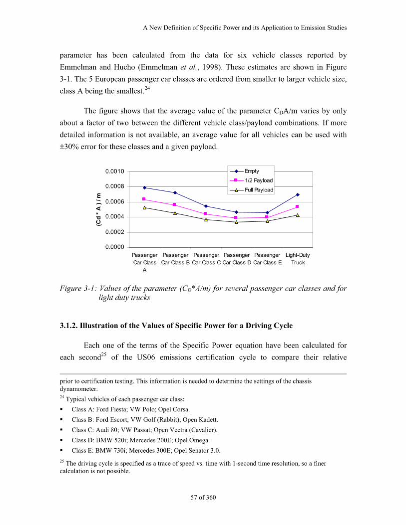
A New Definition of Specific Power and its Application to Emission Studies

57 of 360

parameter has been calculated from the data for six vehicle classes reported by

Emmelman and Hucho (Emmelman et al., 1998). These estimates are shown in Figure

3-1. The 5 European passenger car classes are ordered from smaller to larger vehicle size,

class A being the smallest.24

The figure shows that the average value of the parameter CDA/m varies by only

about a factor of two between the different vehicle class/payload combinations. If more

detailed information is not available, an average value for all vehicles can be used with

±30% error for these classes and a given payload.

0.0000

0.0002

0.0004

0.0006

0.0008

0.0010

PassengerCar Class

A

PassengerCar Class B

PassengerCar Class C

PassengerCar Class D

PassengerCar Class E

Light-DutyTruck

(Cd

* A

) /

m

Empty

1/2 Payload

Full Payload

Figure 3-1: Values of the parameter (CD*A/m) for several passenger car classes and forlight duty trucks

3.1.2. Illustration of the Values of Specific Power for a Driving Cycle

Each one of the terms of the Specific Power equation have been calculated for

each second25 of the US06 emissions certification cycle to compare their relative

prior to certification testing. This information is needed to determine the settings of the chassisdynamometer.24 Typical vehicles of each passenger car class:

Class A: Ford Fiesta; VW Polo; Opel Corsa.

Class B: Ford Escort; VW Golf (Rabbit); Open Kadett.

Class C: Audi 80; VW Passat; Open Vectra (Cavalier).

Class D: BMW 520i; Mercedes 200E; Opel Omega.

Class E: BMW 730i; Mercedes 300E; Opel Senator 3.0.

25 The driving cycle is specified as a trace of speed vs. time with 1-second time resolution, so a finercalculation is not possible.

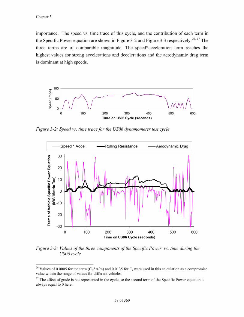
Chapter 3

58 of 360

importance. The speed vs. time trace of this cycle, and the contribution of each term in

the Specific Power equation are shown in Figure 3-2 and Figure 3-3 respectively.26, 27 The

three terms are of comparable magnitude. The speed*acceleration term reaches the

highest values for strong accelerations and decelerations and the aerodynamic drag term

is dominant at high speeds.

0

50

100

0 100 200 300 400 500 600

Time on US06 Cycle (seconds)

Sp

eed

(m

ph

)

Figure 3-2: Speed vs. time trace for the US06 dynamometer test cycle

-30

-20

-10

0

10

20

30

0 100 200 300 400 500 600Time on US06 Cycle (seconds)

Te

rms

of

Ve

hic

le S

pe

cif

ic P

ow

er

Eq

ua

tio

n

(kW

/ M

etr

ic T

on

)

Speed * Accel. Rolling Resistance Aerodynamic Drag

Figure 3-3: Values of the three components of the Specific Power vs. time during theUS06 cycle

26 Values of 0.0005 for the term (CD*A/m) and 0.0135 for Cr were used in this calculation as a compromisevalue within the range of values for different vehicles.27 The effect of grade is not represented in the cycle, so the second term of the Specific Power equation isalways equal to 0 here.

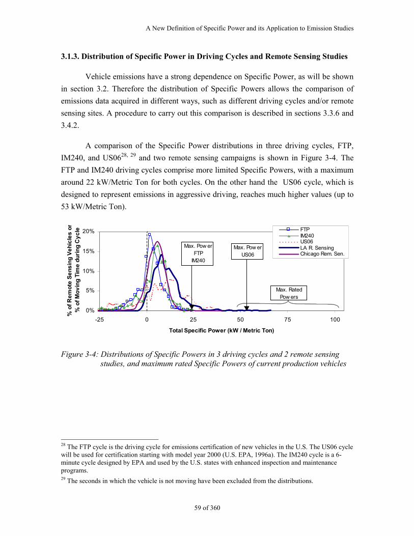
A New Definition of Specific Power and its Application to Emission Studies

59 of 360

3.1.3. Distribution of Specific Power in Driving Cycles and Remote Sensing Studies

Vehicle emissions have a strong dependence on Specific Power, as will be shown

in section 3.2. Therefore the distribution of Specific Powers allows the comparison of

emissions data acquired in different ways, such as different driving cycles and/or remote

sensing sites. A procedure to carry out this comparison is described in sections 3.3.6 and

3.4.2.

A comparison of the Specific Power distributions in three driving cycles, FTP,

IM240, and US0628, 29 and two remote sensing campaigns is shown in Figure 3-4. The

FTP and IM240 driving cycles comprise more limited Specific Powers, with a maximum

around 22 kW/Metric Ton for both cycles. On the other hand the US06 cycle, which is

designed to represent emissions in aggressive driving, reaches much higher values (up to

53 kW/Metric Ton).

0%

5%

10%

15%

20%

-25 0 25 50 75 100

Total Specific Power (kW / Metric Ton)

% o

f R

em

ote

Se

ns

ing

Ve

hic

les

or

% o

f M

ov

ing

Tim

e d

uri

ng

Cy

cle FTP

IM240US06LA R. SensingChicago Rem. Sen.

Max. Pow erFTP

IM240

Max. Rated Pow ers

Max. Pow erUS06

Figure 3-4: Distributions of Specific Powers in 3 driving cycles and 2 remote sensingstudies, and maximum rated Specific Powers of current production vehicles

28 The FTP cycle is the driving cycle for emissions certification of new vehicles in the U.S. The US06 cyclewill be used for certification starting with model year 2000 (U.S. EPA, 1996a). The IM240 cycle is a 6-minute cycle designed by EPA and used by the U.S. states with enhanced inspection and maintenanceprograms.29 The seconds in which the vehicle is not moving have been excluded from the distributions.

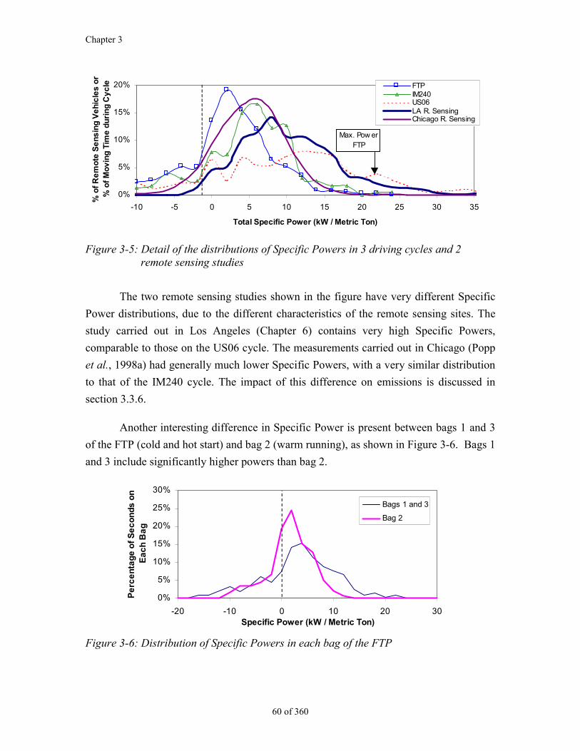
Chapter 3

60 of 360

0%

5%

10%

15%

20%

-10 -5 0 5 10 15 20 25 30 35

Total Specific Power (kW / Metric Ton)

% o

f R

em

ote

Se

ns

ing

Ve

hic

les

or

% o

f M

ov

ing

Tim

e d

uri

ng

Cy

cle FTP

IM240US06LA R. SensingChicago R. Sensing

Max. Pow erFTP

Figure 3-5: Detail of the distributions of Specific Powers in 3 driving cycles and 2remote sensing studies

The two remote sensing studies shown in the figure have very different Specific

Power distributions, due to the different characteristics of the remote sensing sites. The

study carried out in Los Angeles (Chapter 6) contains very high Specific Powers,

comparable to those on the US06 cycle. The measurements carried out in Chicago (Popp

et al., 1998a) had generally much lower Specific Powers, with a very similar distribution

to that of the IM240 cycle. The impact of this difference on emissions is discussed in

section 3.3.6.

Another interesting difference in Specific Power is present between bags 1 and 3

of the FTP (cold and hot start) and bag 2 (warm running), as shown in Figure 3-6. Bags 1

and 3 include significantly higher powers than bag 2.

0%

5%

10%

15%

20%

25%

30%

-20 -10 0 10 20 30Specific Power (kW / Metric Ton)

Pe

rce

nta

ge

of

Se

co

nd

s o

n

Ea

ch

Ba

g

Bags 1 and 3

Bag 2

Figure 3-6: Distribution of Specific Powers in each bag of the FTP

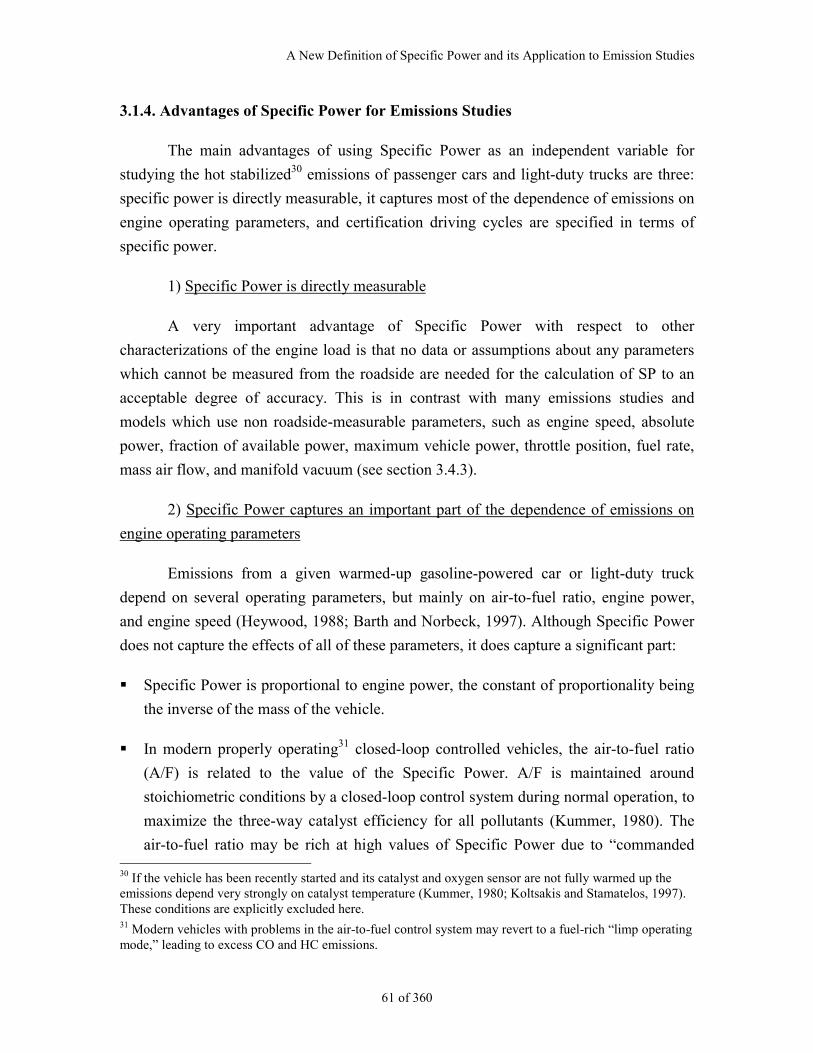
A New Definition of Specific Power and its Application to Emission Studies

61 of 360

3.1.4. Advantages of Specific Power for Emissions Studies

The main advantages of using Specific Power as an independent variable for

studying the hot stabilized30 emissions of passenger cars and light-duty trucks are three:

specific power is directly measurable, it captures most of the dependence of emissions on

engine operating parameters, and certification driving cycles are specified in terms of

specific power.

1) Specific Power is directly measurable

A very important advantage of Specific Power with respect to other

characterizations of the engine load is that no data or assumptions about any parameters

which cannot be measured from the roadside are needed for the calculation of SP to an

acceptable degree of accuracy. This is in contrast with many emissions studies and

models which use non roadside-measurable parameters, such as engine speed, absolute

power, fraction of available power, maximum vehicle power, throttle position, fuel rate,

mass air flow, and manifold vacuum (see section 3.4.3).

2) Specific Power captures an important part of the dependence of emissions on

engine operating parameters

Emissions from a given warmed-up gasoline-powered car or light-duty truck

depend on several operating parameters, but mainly on air-to-fuel ratio, engine power,

and engine speed (Heywood, 1988; Barth and Norbeck, 1997). Although Specific Power

does not capture the effects of all of these parameters, it does capture a significant part:

Specific Power is proportional to engine power, the constant of proportionality being

the inverse of the mass of the vehicle.

In modern properly operating31 closed-loop controlled vehicles, the air-to-fuel ratio

(A/F) is related to the value of the Specific Power. A/F is maintained around

stoichiometric conditions by a closed-loop control system during normal operation, to

maximize the three-way catalyst efficiency for all pollutants (Kummer, 1980). The

air-to-fuel ratio may be rich at high values of Specific Power due to “commanded 30 If the vehicle has been recently started and its catalyst and oxygen sensor are not fully warmed up theemissions depend very strongly on catalyst temperature (Kummer, 1980; Koltsakis and Stamatelos, 1997).These conditions are explicitly excluded here.31 Modern vehicles with problems in the air-to-fuel control system may revert to a fuel-rich “limp operatingmode,” leading to excess CO and HC emissions.

Chapter 3

62 of 360

enrichment“ events (see section 3.3) and lean for negative values due to “fuel cut-off”

events (Haskew et al., 1994; An et al., 1997).

The new definition of Specific Power given in section 3.1 includes the effects of

roadway grades, rolling resistance, and aerodynamic resistance that earlier definitions

of specific power omitted (U.S. EPA, 1993a; Webster et al., 1996; Carlson et al.,

1997). EPA recently estimated that about 45% of the vehicle-miles traveled in the

U.S. take place in grades larger than 1%32, 33 (U.S. EPA, 1993a), and driving on uphill

grades can increase emissions by a factor of two (Cicero-Fernandez et al., 1995;

Cicero-Fernandez et al., 1996). Despite these facts, neither the current EPA emissions

model, (MOBILE5), nor the version currently under development (MOBILE6), nor

California’s emission model (EMFAC) include the effect of roadway grade

(Beardsley, 1998; Long, 1998).

Effects with an influence on emissions that are not captured by the new definition

of Specific Power are:

Engine speed. Although some attempts to model the engine speed of a passing vehicle

have been pursued (Barth et al., 1998), there is no accurate way to estimate this

parameter due to the many different gear systems used. Fortunately the dependence of

emissions on engine speed at a given power is limited (Heywood, 1988; De Soete,

1989).

Engine friction losses. These losses could be modeled (Barth et al., 1997)34 but they

are generally small compared to the range of specific powers of interest.

Transmission losses. The efficiency of automatic transmissions can vary significantly.

Most of this variability is associated with torque converter slip. The definition of SP

given here ignores this loss and makes no distinction between automatic and manual

transmissions. The overall effect of the transmission slip on the SP is expected to be

32 Half on positive grade and half on negative grade. A grade of ±1% at 50 mph contributes ±2.2kW/Metric Ton to the Specific Power, or 1/10 of the maximum FTP SP value.33 Data from Germany indicate a similar prevalence of roadway grades (Emmelman et al., 1998).34 The model proposed by Barth et al. (Barth et al., 1997) is Pfriction = φ * K * N * V, where φ is the fuel toair ratio, k is the engine friction factor, N is the engine speed, and V is the engine displacement. Thus themodel of the friction losses depends on three non-measurable parameters (φ could be determined from theemission meausrements.

A New Definition of Specific Power and its Application to Emission Studies

63 of 360

small except when a vehicle is accelerating from low speed and slip is high (Koplow,

1998).

Power consumption of accessories such as air conditioning. Air conditioning in

particular can impose an important extra load on the engine, which translates into

an increase of emissions.35 The fraction of the fleet equipped with air conditioning

reaches more than 90% for model year 1996 (Koupal, 1998). For these reasons,

models of the load imposed by air conditioning as a function of environmental

conditions (temperature, humidity, solar load) are being developed (Koupal,

1998) and could be added to the calculation of Specific Power.36

Payload weight. The maximum payload of a passenger car or light-duty truck

varies from about 30% to 60% of the vehicle’s weight (Emmelman et al., 1998).

This means that two vehicles of the same model with the same Specific Power

could have such differences in absolute power depending on how many

passengers and load a given vehicle is carrying.37 An analysis of this effect is

presented in section 3.2.6.

It is possible in principle to determine the mass of a vehicle during remote sensing

with a “weight-in-motion” measurement system (U.S. DOT, 1997b). Then engine

power could be calculated by multiplying Specific Power by the measured mass.

However, it is not clear that knowing the absolute power instead of Specific Power

will provide better information for remote sensing and emissions models (see sections

3.2.5 and 3.2.6), so the cost of such a system may not be justified.38

35 For this reason the emissions under A/C use have recently been regulated. Starting with model year 2000,new cars and light-duty trucks will be tested on the SC03 cycle, which is designed to represent the effectsof air conditioning (U.S. EPA, 1996a).36 Prof. Stedman suggested a strategy to determine which vehicles had air conditioners on in the summer: asecond video camera which records whether the driver’s side window is up. On hot days this could be agood predictor of whether the air conditioner is on (Slott, 1997).37 In our remote sensing study (Chapter 6) we measured mostly commuter vehicles and observed that a verylarge fraction only had one or two occupants. A possible strategy to screening out part of the effects ofextra weight in remote sensing studies would be to use a second video camera and reject the measurementsdone on vehicles with high occupancy.38 The cost of a weight-in motion system for heavy-duty trucks was calculated to be about $20,000 per sitefor a state implementing 100 sites (U.S. DOT, 1997b). This cost will be certainly higher for a singleportable system adapted to passenger cars and light-duty trucks.

Chapter 3

64 of 360

Large increases in aerodynamic drag due to roof racks or for high drag vehicles such

as convertibles.39 These will only be important at high speeds due to the dependence

of the aerodynamic power dissipation term on the cube of the vehicle speed.40

Effects of cross-winds on the aerodynamic drag coefficient. CD generally

increases when the effective wind is not in the same direction of vehicle

travel (Barnard, 1996; SAE, 1996). This increase can reach 14% (20%) for

cars (vans) (Barnard, 1996).41

History effects over several seconds on the engine and the catalyst (An et

al., 1997; Nam and Ross, 1998). These appear because the engine-catalyst

system can have some “memory” of past events, e.g. extra fuel may be left

on the intake port from a recent commanded enrichment event, or the

oxygen storage in the catalyst may have changed due to recent rich or lean

operation.

3) Emissions certification test cycles specify Specific Power directly

A key fact that makes Specific Power very useful for emissions studies is that the

driving cycles that are used for emissions testing and certification of passenger cars and

light-duty trucks specify Specific Power vs. time directly. This due to the fact that all

chassis dynamometer driving cycles used for emissions certification testing in the US,

Europe, and Japan are defined as a speed vs. time trace (Bauer, 1996; U.S. EPA, 1996a).

Acceleration is implicitly specified as well, since it is just the derivative of the speed vs.

time curve. Since driving cycles do not include any simulation of roadway grade effects,

the equation in section 3.1 implies that Specific Power is defined at each second for a

given vehicle.42, 43

There is evidence that vehicle emission control strategies are optimized for the

test cycles. Principal evidence is the threshold for commanded enrichment incorporated 39 Typical drag coefficients for convertibles are on the range 0.5-0.7, as compared to 0.25-0.4 for normalcars (Bauer, 1996).40 Experimental values for CD (Emmelman et al., 1998) could be used in these cases.41 This increase reaches 60% for articulated heavy-duty trucks (Barnard, 1996).42 Chassis dynamometer cycles match the load encountered a vehicle on the road for a given speed andacceleration with simulated vehicle-specific loads for aerodynamic and rolling resistance and vehicleinertia (Haskew et al., 1994).43 However significant differences in Specific Power can exist within the acceptable tolerances of thedriving cycle, leading to significant differences in emissions (Webster et al., 1996).

A New Definition of Specific Power and its Application to Emission Studies

65 of 360

into the control strategies of vehicles, which starts to occur above the maximum Specific

Power of the FTP certification cycle for vehicles with very different maximum rated

Specific Powers (see sections 3.2.4 and 3.3.4). Another piece of evidence is the recent

settlement in which seven heavy duty diesel engine manufacturers agreed to a penalty

exceeding $1 billion for designing their emission control systems to pass the regulatory

test for NOx while not, according to the EPA, sufficiently reducing on highway emissions

(U.S. EPA, 1998b).

In conclusion: Specific Power is directly measurable and is a good predictor of

vehicle emissions. This predictive ability is demonstrated in section 3.2 by analyzing

second-by-second data taken on test vehicles during chassis dynamometer testing.

However, instantaneous vehicle emissions are not just a “state function” of Specific

Power. Rather instantaneous Specific Power should be used as the main variable

representing engine load in emission studies, although the history or statistics of Specific

Power, or other additional input variables may be needed to properly describe or model

all situations.

Chapter 3

66 of 360

3.2. Analysis of Second-by-Second Emissions Data vs. SpecificPower

3.2.1. Second-by-Second Emissions Data

Second-by-second emissions data from 68 vehicles of model years 1991-1996

recently tested on several driving cycles are publicly available (Liberty et al., 1997).44

These data include one second averages of vehicle speed, fuel economy, engine-out and

tailpipe CO, HC, and NOx emissions, catalyst and exhaust temperature, and engine speed.

Very high power demands are included because the tests were designed to help quantify

the emissions of current vehicles under aggressive driving conditions.

The analysis presented in the following sections is based on the use of these

second-by-second data.45, 46 The main objective of this analysis is to show that emissions

are closely related to Specific Power, and that this relationship is stronger than that of

other commonly used predictive parameters for vehicle emissions.

3.2.2. Variations of the Emissions Results of Different Driving Cycles vs. Specific

Power

The relationship between the second-by-second CO, HC, and NOx engine-out

(uncatalyzed), and tailpipe (catalyzed) emissions and Specific Power for a recent

production vehicle tested on a dynamometer driving cycle are shown in Figure 3-7.

Specific Power was calculated with the equation given in section 3.1 from the one

second average speed and a finite difference approximation of the acceleration.

Additional graphs showing these same emissions vs. SP for two repetitions of four

different driving cycles are included in Appendix B for reference.

44 These emissions data were acquired as part of an EPA-industry effort to design the new regulations tolimit emissions that occurred in driving modes not represented on the Federal Test Procedure driving cycle(FTP). These studies resulted in a redesign of the U.S. emission standards (U.S. EPA, 1996a), with twonew driving cycles being required to limit emissions under aggressive driving (US06 cycle, shown inFigure 3-2) and with air conditioner use.45 A value of 0.0135 for Cr and 0.0005 for (CD*A)/m has been used for all vehicles in this section.46 An important limitation of this data set is the imprecision calculation of acceleration. Acceleration hasbeen calculated as a centered finite difference derivative of speed. Using this procedure with 1 Hz data may“smooth out” significant changes in acceleration which happen on time scales shorter than 1 second.Driving cycle data acquired at 10 Hz instead of 1 Hz would be much more adequate for the purposes of thisstudy. Unfortunately, and although the data in from SFTP program analyzed here were indeed acquired at10 Hz (Haskew et al., 1994), only the 1 Hz averaged data are available (Haskew, 1998). Two automobilemanufacturers were contacted but were also unable to provide a data set of this kind taken at 10 Hz.

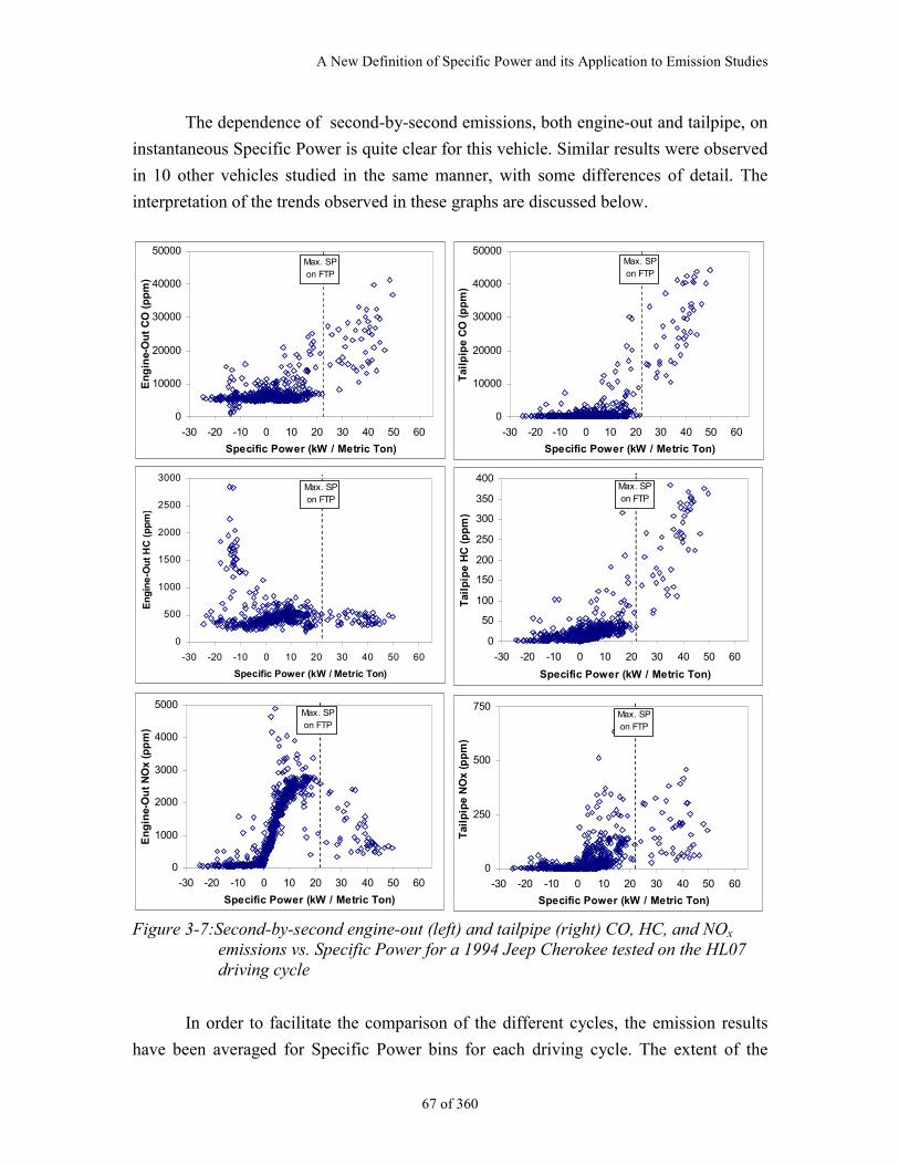
A New Definition of Specific Power and its Application to Emission Studies

67 of 360

The dependence of second-by-second emissions, both engine-out and tailpipe, on

instantaneous Specific Power is quite clear for this vehicle. Similar results were observed

in 10 other vehicles studied in the same manner, with some differences of detail. The

interpretation of the trends observed in these graphs are discussed below.

0

10000

20000

30000

40000

50000

-30 -20 -10 0 10 20 30 40 50 60

Specific Power (kW / Metric Ton)

En

gin

e-O

ut

CO

(p

pm

)

Max. SP on FTP

0

10000

20000

30000

40000

50000

-30 -20 -10 0 10 20 30 40 50 60

Specific Power (kW / Metric Ton)T

ailp

ipe

CO

(p

pm

)

Max. SP on FTP

0

500

1000

1500

2000

2500

3000

-30 -20 -10 0 10 20 30 40 50 60

Specific Power (kW / Metric Ton)

En

gin

e-O

ut

HC

(p

pm

)

Max. SP on FTP

0

50

100

150

200

250

300

350

400

-30 -20 -10 0 10 20 30 40 50 60

Specific Power (kW / Metric Ton)

Tai

lpip

e H

C (

pp

m)

Max. SP on FTP

0

1000

2000

3000

4000

5000

-30 -20 -10 0 10 20 30 40 50 60

Specific Power (kW / Metric Ton)

En

gin

e-O

ut

NO

x (p

pm

)

Max. SP on FTP

0

250

500

750

-30 -20 -10 0 10 20 30 40 50 60

Specific Power (kW / Metric Ton)

Tai

lpip

e N

Ox

(pp

m)

Max. SP on FTP

Figure 3-7:Second-by-second engine-out (left) and tailpipe (right) CO, HC, and NOx

emissions vs. Specific Power for a 1994 Jeep Cherokee tested on the HL07driving cycle

In order to facilitate the comparison of the different cycles, the emission results

have been averaged for Specific Power bins for each driving cycle. The extent of the

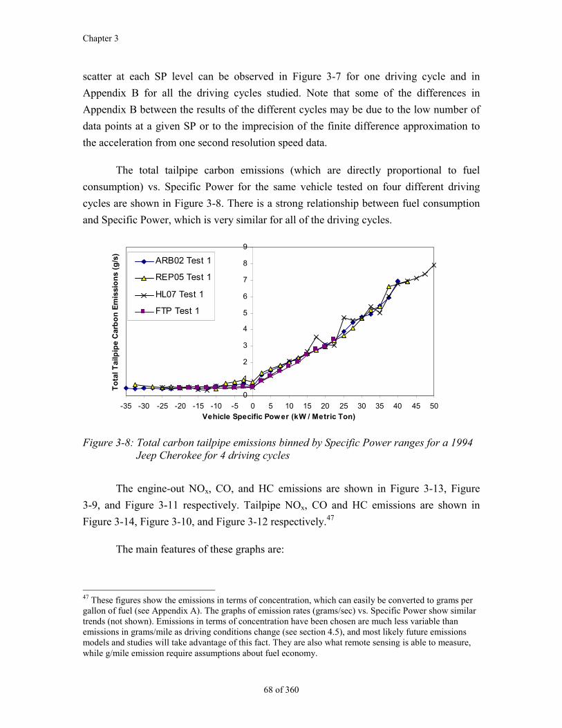
Chapter 3

68 of 360

scatter at each SP level can be observed in Figure 3-7 for one driving cycle and in

Appendix B for all the driving cycles studied. Note that some of the differences in

Appendix B between the results of the different cycles may be due to the low number of

data points at a given SP or to the imprecision of the finite difference approximation to

the acceleration from one second resolution speed data.

The total tailpipe carbon emissions (which are directly proportional to fuel

consumption) vs. Specific Power for the same vehicle tested on four different driving

cycles are shown in Figure 3-8. There is a strong relationship between fuel consumption

and Specific Power, which is very similar for all of the driving cycles.

0

1

2

3

4

5

6

7

8

9

-35 -30 -25 -20 -15 -10 -5 0 5 10 15 20 25 30 35 40 45 50

Vehicle Specific Power (kW / Metric Ton)

To

tal T

ailp

ipe

Car

bo

n E

mis

sio

ns

(g/s

)

ARB02 Test 1

REP05 Test 1

HL07 Test 1

FTP Test 1

Figure 3-8: Total carbon tailpipe emissions binned by Specific Power ranges for a 1994Jeep Cherokee for 4 driving cycles

The engine-out NOx, CO, and HC emissions are shown in Figure 3-13, Figure

3-9, and Figure 3-11 respectively. Tailpipe NOx, CO and HC emissions are shown in

Figure 3-14, Figure 3-10, and Figure 3-12 respectively.47

The main features of these graphs are:

47 These figures show the emissions in terms of concentration, which can easily be converted to grams pergallon of fuel (see Appendix A). The graphs of emission rates (grams/sec) vs. Specific Power show similartrends (not shown). Emissions in terms of concentration have been chosen are much less variable thanemissions in grams/mile as driving conditions change (see section 4.5), and most likely future emissionsmodels and studies will take advantage of this fact. They are also what remote sensing is able to measure,while g/mile emission require assumptions about fuel economy.

A New Definition of Specific Power and its Application to Emission Studies

69 of 360

Engine-out CO emissions stay at a value of about 0.6% for Specific Powers below the

maximum FTP SP (~22 kW/Metric Ton). This levels are typical of stoichiometric

combustion conditions (Heywood, 1988). Much larger CO emissions appear beyond

the maximum FTP Specific Powers most likely due to the use of commanded

enrichment.

Engine-out HC emissions stay almost constant at about 500 ppm in all the cases

presented here for all positive Specific Powers and driving cycles. These emissions

do not increase appreciably during commanded enrichment situations. On the other

hand, HC emissions increase for very negative SP in some cycles, during rapid or

prolonged decelerations.48

“Fuel cut-off” is a commonly used engine management strategy during decelerations

to reduce HC emissions. Consequently, the fuel left on the engine manifold forms

lean mixtures in the engine with poor combustion and high HC emissions (An et al.,

1997). “Manifold flash” happens when the throttle is suddenly closed and the liquid

fuel present on the intake port vaporizes due to the drop in manifold pressure

(Haskew et al., 1994).49

Engine-out NOx emissions are low for negative Specific Powers due to the lower

combustion temperatures, and increase rapidly with Specific Power up to about 2500

ppm.50 NOx concentrations decrease at Specific Powers larger than the maximum

values on the FTP, due to commanded enrichment.

Tailpipe emissions are also similarly clustered for the different driving cycles, with

somewhat larger differences for NOx emissions. Note that tailpipe HC emissions

increase appreciably under commanded enrichment, even though engine-out HC

48 An and Scora (An et al., 1997) found a threshold on the rate of change of specific power (defined as2*speed*acceleration) above which high HC emissions did not occur during rapid load reduction event in15 test vehicles. This threshold is –50 mph2/sec2, or –10 kW/Metric Ton/second in metric units. It may bedifficult to measure this parameter in remote sensing since it involves the derivative of the acceleration.These researchers also estimated that these emissions accounted for 25%-30% of the total HC on theMEC01 and US06 cycles.49 This discussion focuses on modern port fuel-injected vehicles. Earlier fuel delivery technologies such asthrottle-body fuel injection or carburetors would produce higher HC emissions since there is more room forfuel accumulation due to the longer distance from the fuel introduction point to the engine cylinders, whichleaves more room for fuel accumulation.50 This particular vehicle was not equipped with an Exhaust Gas Recirculation (EGR) system to reduceengine-out NOx emissions.

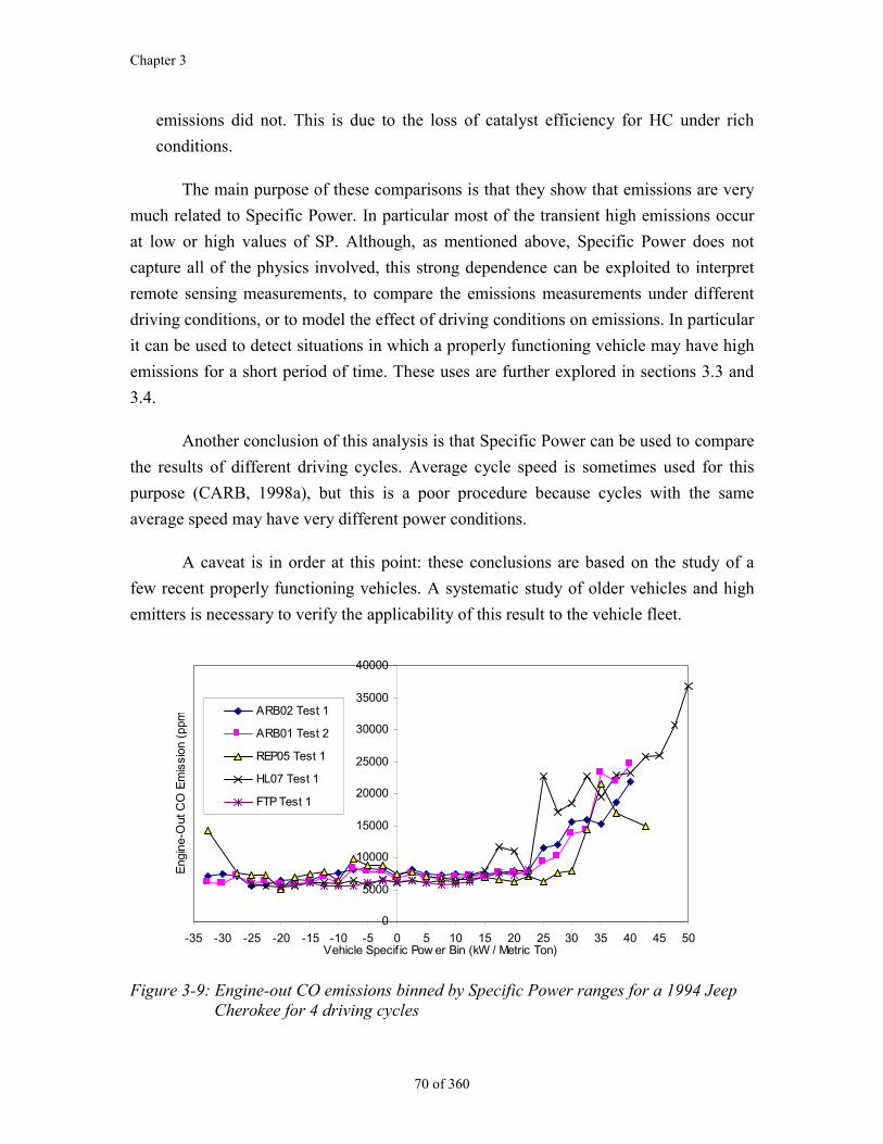
Chapter 3

70 of 360

emissions did not. This is due to the loss of catalyst efficiency for HC under rich

conditions.

The main purpose of these comparisons is that they show that emissions are very

much related to Specific Power. In particular most of the transient high emissions occur

at low or high values of SP. Although, as mentioned above, Specific Power does not

capture all of the physics involved, this strong dependence can be exploited to interpret

remote sensing measurements, to compare the emissions measurements under different

driving conditions, or to model the effect of driving conditions on emissions. In particular

it can be used to detect situations in which a properly functioning vehicle may have high

emissions for a short period of time. These uses are further explored in sections 3.3 and

3.4.

Another conclusion of this analysis is that Specific Power can be used to compare

the results of different driving cycles. Average cycle speed is sometimes used for this

purpose (CARB, 1998a), but this is a poor procedure because cycles with the same

average speed may have very different power conditions.

A caveat is in order at this point: these conclusions are based on the study of a

few recent properly functioning vehicles. A systematic study of older vehicles and high

emitters is necessary to verify the applicability of this result to the vehicle fleet.

0

5000

10000

15000

20000

25000

30000

35000

40000

-35 -30 -25 -20 -15 -10 -5 0 5 10 15 20 25 30 35 40 45 50Vehicle Specif ic Pow er Bin (kW / Metric Ton)

Eng

ine-

Out

CO

Em

issi

on (

ppm

ARB02 Test 1

ARB01 Test 2

REP05 Test 1

HL07 Test 1

FTP Test 1

Figure 3-9: Engine-out CO emissions binned by Specific Power ranges for a 1994 JeepCherokee for 4 driving cycles

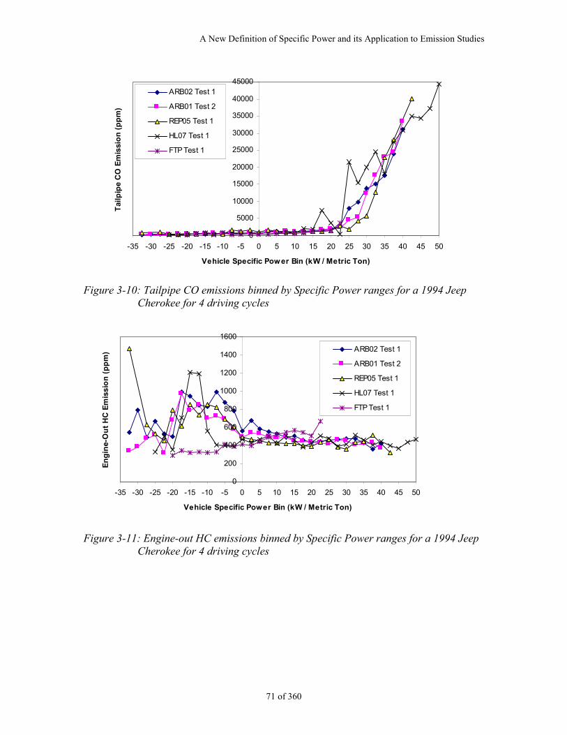
A New Definition of Specific Power and its Application to Emission Studies

71 of 360

0

5000

10000

15000

20000

25000

30000

35000

40000

45000

-35 -30 -25 -20 -15 -10 -5 0 5 10 15 20 25 30 35 40 45 50

Vehicle Specific Power Bin (kW / Metric Ton)

Tai

lpip

e C

O E

mis

sio

n (

pp

m)

ARB02 Test 1

ARB01 Test 2

REP05 Test 1

HL07 Test 1

FTP Test 1

Figure 3-10: Tailpipe CO emissions binned by Specific Power ranges for a 1994 JeepCherokee for 4 driving cycles

0

200

400

600

800

1000

1200

1400

1600

-35 -30 -25 -20 -15 -10 -5 0 5 10 15 20 25 30 35 40 45 50

Vehicle Specific Power Bin (kW / Metric Ton)

En

gin

e-O

ut

HC

Em

issi

on

(p

pm

) ARB02 Test 1

ARB01 Test 2

REP05 Test 1

HL07 Test 1

FTP Test 1

Figure 3-11: Engine-out HC emissions binned by Specific Power ranges for a 1994 JeepCherokee for 4 driving cycles

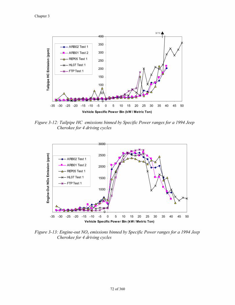
Chapter 3

72 of 360

0

50

100

150

200

250

300

350

400

-35 -30 -25 -20 -15 -10 -5 0 5 10 15 20 25 30 35 40 45 50

Vehicle Specific Power Bin (kW / Metric Ton)

Tai

lpip

e H

C E

mis

sio

n (

pp

m) ARB02 Test 1

ARB01 Test 2

REP05 Test 1

HL07 Test 1

FTP Test 1

1079

Figure 3-12: Tailpipe HC emissions binned by Specific Power ranges for a 1994 JeepCherokee for 4 driving cycles

0

500

1000

1500

2000

2500

3000

-35 -30 -25 -20 -15 -10 -5 0 5 10 15 20 25 30 35 40 45 50

Vehicle Specific Power Bin (kW / Metric Ton)

En

gin

e-O

ut

NO

x E

mis

sio

n (

pp

m)

ARB02 Test 1

ARB01 Test 2

REP05 Test 1

HL07 Test 1

FTP Test 1

Figure 3-13: Engine-out NOx emissions binned by Specific Power ranges for a 1994 JeepCherokee for 4 driving cycles

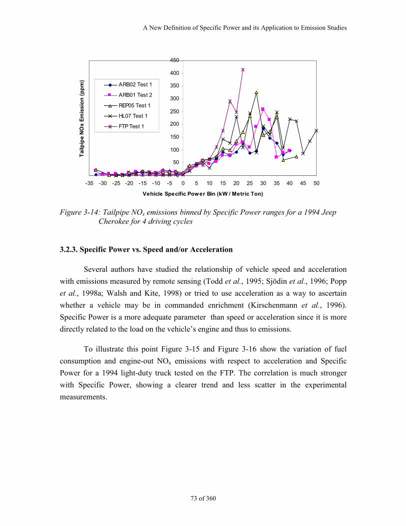
A New Definition of Specific Power and its Application to Emission Studies

73 of 360

0

50

100

150

200

250

300

350

400

450

-35 -30 -25 -20 -15 -10 -5 0 5 10 15 20 25 30 35 40 45 50

Vehicle Specific Power Bin (kW / Metric Ton)

Tai

lpip

e N

Ox

Em

issi

on

(p

pm

)ARB02 Test 1

ARB01 Test 2

REP05 Test 1

HL07 Test 1

FTP Test 1

Figure 3-14: Tailpipe NOx emissions binned by Specific Power ranges for a 1994 JeepCherokee for 4 driving cycles

3.2.3. Specific Power vs. Speed and/or Acceleration

Several authors have studied the relationship of vehicle speed and acceleration

with emissions measured by remote sensing (Todd et al., 1995; Sjödin et al., 1996; Popp

et al., 1998a; Walsh and Kite, 1998) or tried to use acceleration as a way to ascertain

whether a vehicle may be in commanded enrichment (Kirschenmann et al., 1996).

Specific Power is a more adequate parameter than speed or acceleration since it is more

directly related to the load on the vehicle’s engine and thus to emissions.

To illustrate this point Figure 3-15 and Figure 3-16 show the variation of fuel

consumption and engine-out NOx emissions with respect to acceleration and Specific

Power for a 1994 light-duty truck tested on the FTP. The correlation is much stronger

with Specific Power, showing a clearer trend and less scatter in the experimental

measurements.

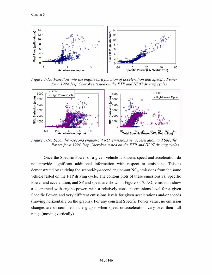
Chapter 3

74 of 360

0

2

4

6

8

10

12

14

-4 1 6Acceleration (mph/s)

Fu

el

Flo

w (

ga

llo

n/h

ou

r)

0

2

4

6

8

10

12

14

-20 0 20 40 60Specific Power (kW / Metric Ton)

Fu

el

Flo

w (

ga

llo

n/h

ou

r)

Figure 3-15: Fuel flow into the engine as a function of acceleration and Specific Powerfor a 1994 Jeep Cherokee tested on the FTP and HL07 driving cycles

0

1000

2000

3000

4000

5000

6000

-5.0 -2.5 0.0 2.5 5.0Acceleration (mph/s)

NO

x E

mis

sio

n (

pp

m)

FTPHigh Power Cycle

0

1000

2000

3000

4000

5000

6000

-10 0 10 20 30 40 50 60Total Specific Power (kW / Metric Ton)

NO

x E

mis

sio

n (

pp

m)

FTP

High Power Cycle

Figure 3-16: Second-by-second engine-out NOx emissions vs. acceleration and SpecificPower for a 1994 Jeep Cherokee tested on the FTP and HL07 driving cycles

Once the Specific Power of a given vehicle is known, speed and acceleration do

not provide significant additional information with respect to emissions. This is

demonstrated by studying the second-by-second engine-out NOx emissions from the same

vehicle tested on the FTP driving cycle. The contour plots of these emissions vs. Specific

Power and acceleration, and SP and speed are shown in Figure 3-17. NOx emissions show

a clear trend with engine power, with a relatively constant emissions level for a given

Specific Power, and very different emissions levels for given accelerations and/or speeds

(moving horizontally on the graphs). For any constant Specific Power value, no emission

changes are discernible in the graphs when speed or acceleration vary over their full

range (moving vertically).

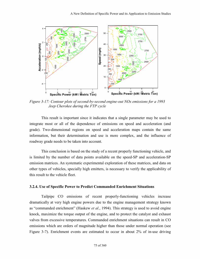
A New Definition of Specific Power and its Application to Emission Studies

75 of 360

-4

-2

0

2

4

Acc

eler

atio

n (

mp

h/s

)

20151050 Specific Power (kW / Metric Ton)

275

0

250

0

2500

225

0

225

0

200

0 2

000

150

0

150

0

100

0 1

000

500

250

250

2

50

100

50

40

30

20

10

0

Sp

eed

(m

ph

)

20151050 Specific Power (kW / Metric Ton)

2750

2750

2750

250

0

2500

2500

2500

2250

2250

2000

2000

1500

1500

1000

1000

500

500

250

250

Figure 3-17: Contour plots of second-by-second engine-out NOx emissions for a 1993Jeep Cherokee during the FTP cycle

This result is important since it indicates that a single parameter may be used to

integrate most or all of the dependence of emissions on speed and acceleration (and

grade). Two-dimensional regions on speed and acceleration maps contain the same

information, but their determination and use is more complex, and the influence of

roadway grade needs to be taken into account.

This conclusion is based on the study of a recent properly functioning vehicle, and

is limited by the number of data points available on the speed-SP and acceleration-SP

emission matrices. An systematic experimental exploration of these matrices, and data on

other types of vehicles, specially high emitters, is necessary to verify the applicability of

this result to the vehicle fleet.

3.2.4. Use of Specific Power to Predict Commanded Enrichment Situations

Tailpipe CO emissions of recent properly-functioning vehicles increase

dramatically at very high engine powers due to the engine management strategy known

as “commanded enrichment” (Haskew et al., 1994). This strategy is used to avoid engine

knock, maximize the torque output of the engine, and to protect the catalyst and exhaust

valves from excessive temperatures. Commanded enrichment situations can result in CO

emissions which are orders of magnitude higher than those under normal operation (see

Figure 3-7). Enrichment events are estimated to occur in about 2% of in-use driving

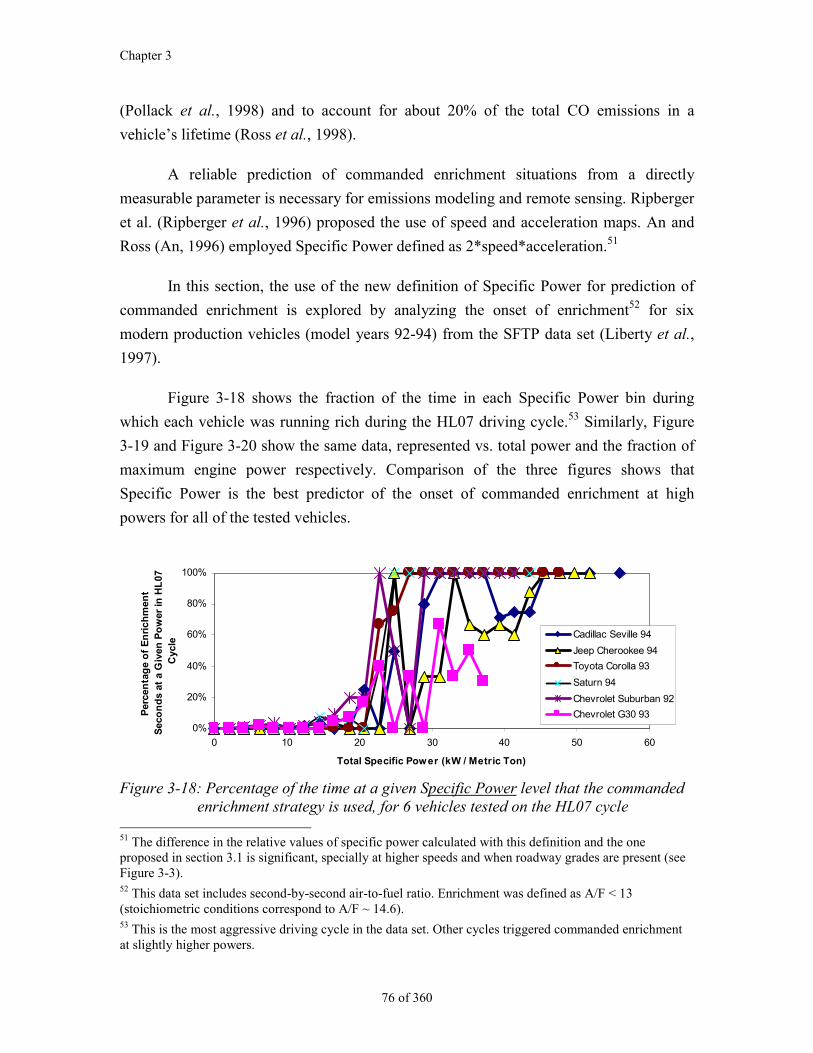
Chapter 3

76 of 360

(Pollack et al., 1998) and to account for about 20% of the total CO emissions in a

vehicle’s lifetime (Ross et al., 1998).

A reliable prediction of commanded enrichment situations from a directly

measurable parameter is necessary for emissions modeling and remote sensing. Ripberger

et al. (Ripberger et al., 1996) proposed the use of speed and acceleration maps. An and

Ross (An, 1996) employed Specific Power defined as 2*speed*acceleration.51

In this section, the use of the new definition of Specific Power for prediction of

commanded enrichment is explored by analyzing the onset of enrichment52 for six

modern production vehicles (model years 92-94) from the SFTP data set (Liberty et al.,

1997).

Figure 3-18 shows the fraction of the time in each Specific Power bin during

which each vehicle was running rich during the HL07 driving cycle.53 Similarly, Figure

3-19 and Figure 3-20 show the same data, represented vs. total power and the fraction of

maximum engine power respectively. Comparison of the three figures shows that

Specific Power is the best predictor of the onset of commanded enrichment at high

powers for all of the tested vehicles.

0%

20%

40%

60%

80%

100%

0 10 20 30 40 50 60

Total Specific Power (kW / Metric Ton)

Per

cen

tag

e o

f E

nri

chm

ent

Sec

on

ds

at a

Giv

en P

ow

er in

HL

07

Cyc

le

Cadillac Seville 94

Jeep Cherookee 94

Toyota Corolla 93

Saturn 94

Chevrolet Suburban 92

Chevrolet G30 93

Figure 3-18: Percentage of the time at a given Specific Power level that the commandedenrichment strategy is used, for 6 vehicles tested on the HL07 cycle

51 The difference in the relative values of specific power calculated with this definition and the oneproposed in section 3.1 is significant, specially at higher speeds and when roadway grades are present (seeFigure 3-3).52 This data set includes second-by-second air-to-fuel ratio. Enrichment was defined as A/F < 13(stoichiometric conditions correspond to A/F ~ 14.6).53 This is the most aggressive driving cycle in the data set. Other cycles triggered commanded enrichmentat slightly higher powers.

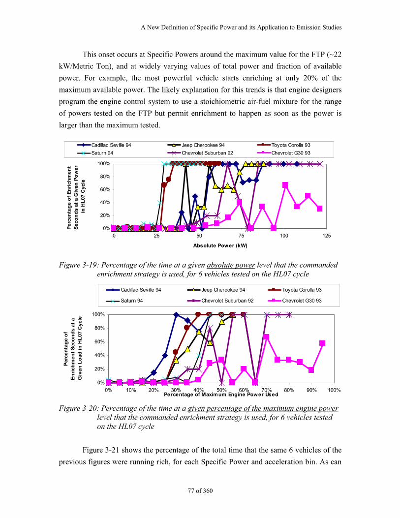
A New Definition of Specific Power and its Application to Emission Studies

77 of 360

This onset occurs at Specific Powers around the maximum value for the FTP (~22

kW/Metric Ton), and at widely varying values of total power and fraction of available

power. For example, the most powerful vehicle starts enriching at only 20% of the

maximum available power. The likely explanation for this trends is that engine designers

program the engine control system to use a stoichiometric air-fuel mixture for the range

of powers tested on the FTP but permit enrichment to happen as soon as the power is

larger than the maximum tested.

0%

20%

40%

60%

80%

100%

0 25 50 75 100 125

Absolute Power (kW)

Per

cen

tag

e o

f E

nri

chm

ent

Sec

on

ds

at a

Giv

en P

ow

er

in H

L07

Cyc

le

Cadillac Seville 94 Jeep Cherookee 94 Toyota Corolla 93

Saturn 94 Chevrolet Suburban 92 Chevrolet G30 93

Figure 3-19: Percentage of the time at a given absolute power level that the commandedenrichment strategy is used, for 6 vehicles tested on the HL07 cycle

0%

20%

40%

60%

80%

100%

0% 10% 20% 30% 40% 50% 60% 70% 80% 90% 100%Percentage of Maximum Engine Power Used

Per

cen

tag

e o

f E

nri

chm

ent

Sec

on

ds

at a

G

iven

Lo

ad in

HL

07 C

ycle

Cadillac Seville 94 Jeep Cherookee 94 Toyota Corolla 93

Saturn 94 Chevrolet Suburban 92 Chevrolet G30 93

Figure 3-20: Percentage of the time at a given percentage of the maximum engine powerlevel that the commanded enrichment strategy is used, for 6 vehicles testedon the HL07 cycle

Figure 3-21 shows the percentage of the total time that the same 6 vehicles of the

previous figures were running rich, for each Specific Power and acceleration bin. As can

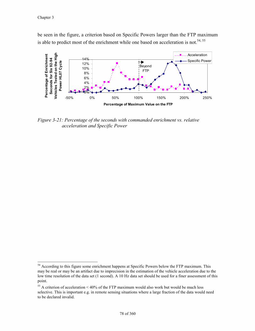
Chapter 3

78 of 360

be seen in the figure, a criterion based on Specific Powers larger than the FTP maximum

is able to predict most of the enrichment while one based on acceleration is not.54, 55

0%2%4%6%

8%10%12%14%

-50% 0% 50% 100% 150% 200% 250%

Percentage of Maximum Value on the FTP

Pe

rce

nta

ge

of

En

ric

hm

en

t S

ec

on

ds

fo

r S

ix 9

2-9

4

Ve

hic

les

Te

ste

d o

n t

he

Hig

h

Po

we

r H

L0

7 C

yc

le

Acceleration

Specific Power

BeyondFTP

Figure 3-21: Percentage of the seconds with commanded enrichment vs. relativeacceleration and Specific Power

54 According to this figure some enrichment happens at Specific Powers below the FTP maximum. Thismay be real or may be an artifact due to imprecision in the estimation of the vehicle acceleration due to thelow time resolution of the data set (1 second). A 10 Hz data set should be used for a finer assessment of thispoint.55 A criterion of acceleration < 40% of the FTP maximum would also work but would be much lessselective. This is important e.g. in remote sensing situations where a large fraction of the data would needto be declared invalid.

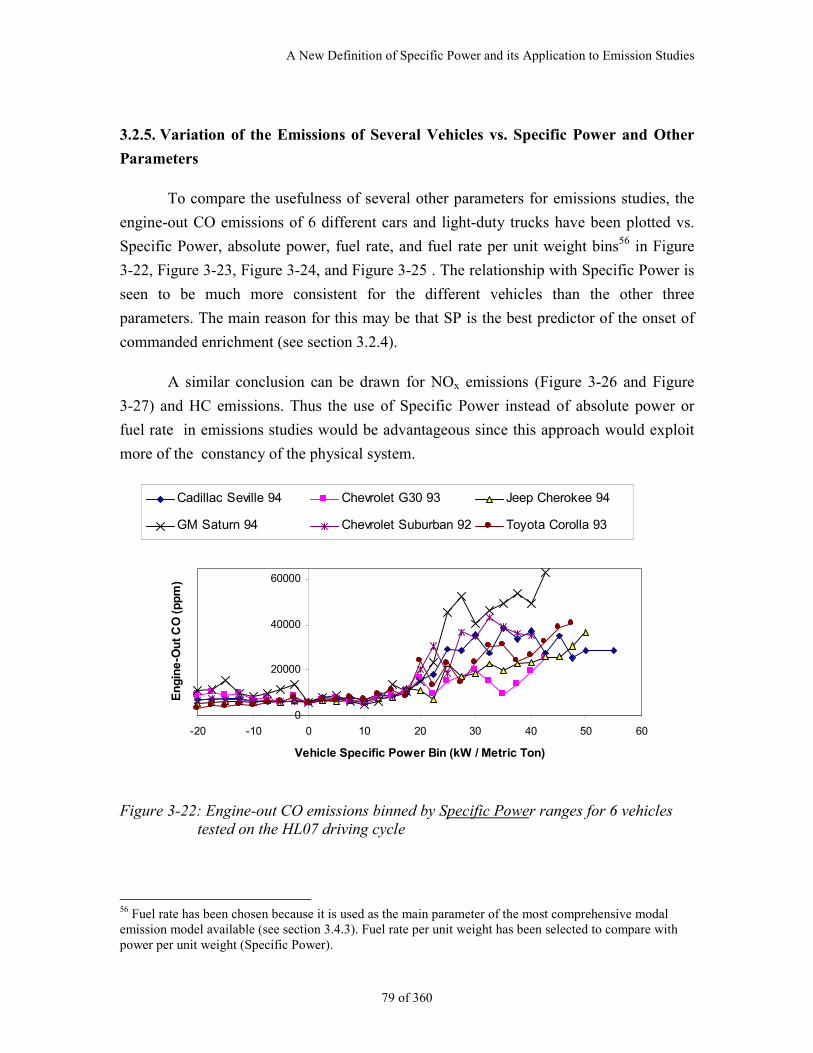
A New Definition of Specific Power and its Application to Emission Studies

79 of 360

3.2.5. Variation of the Emissions of Several Vehicles vs. Specific Power and Other

Parameters

To compare the usefulness of several other parameters for emissions studies, the

engine-out CO emissions of 6 different cars and light-duty trucks have been plotted vs.

Specific Power, absolute power, fuel rate, and fuel rate per unit weight bins56 in Figure

3-22, Figure 3-23, Figure 3-24, and Figure 3-25 . The relationship with Specific Power is

seen to be much more consistent for the different vehicles than the other three

parameters. The main reason for this may be that SP is the best predictor of the onset of

commanded enrichment (see section 3.2.4).

A similar conclusion can be drawn for NOx emissions (Figure 3-26 and Figure

3-27) and HC emissions. Thus the use of Specific Power instead of absolute power or

fuel rate in emissions studies would be advantageous since this approach would exploit

more of the constancy of the physical system.

0

20000

40000

60000

-20 -10 0 10 20 30 40 50 60

Vehicle Specific Power Bin (kW / Metric Ton)

En

gin

e-O

ut

CO

(p

pm

)

Cadillac Seville 94 Chevrolet G30 93 Jeep Cherokee 94

GM Saturn 94 Chevrolet Suburban 92 Toyota Corolla 93

Figure 3-22: Engine-out CO emissions binned by Specific Power ranges for 6 vehiclestested on the HL07 driving cycle

56 Fuel rate has been chosen because it is used as the main parameter of the most comprehensive modalemission model available (see section 3.4.3). Fuel rate per unit weight has been selected to compare withpower per unit weight (Specific Power).

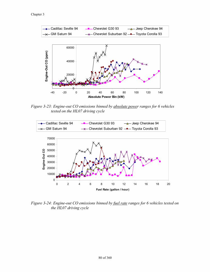
Chapter 3

80 of 360

0

20000

40000

60000

-40 -20 0 20 40 60 80 100 120 140

Absolute Power Bin (kW)

En

gin

e-O

ut

CO

(p

pm

)

Cadillac Seville 94 Chevrolet G30 93 Jeep Cherokee 94

GM Saturn 94 Chevrolet Suburban 92 Toyota Corolla 93

Figure 3-23: Engine-out CO emissions binned by absolute power ranges for 6 vehiclestested on the HL07 driving cycle

0

10000

20000

30000

40000

50000

60000

70000

0 2 4 6 8 10 12 14 16 18 20

Fuel Rate (gallon / hour)

En

gin

e-O

ut

CO

Cadillac Seville 94 Chevrolet G30 93 Jeep Cherokee 94

GM Saturn 94 Chevrolet Suburban 92 Toyota Corolla 93

Figure 3-24: Engine-out CO emissions binned by fuel rate ranges for 6 vehicles tested onthe HL07 driving cycle

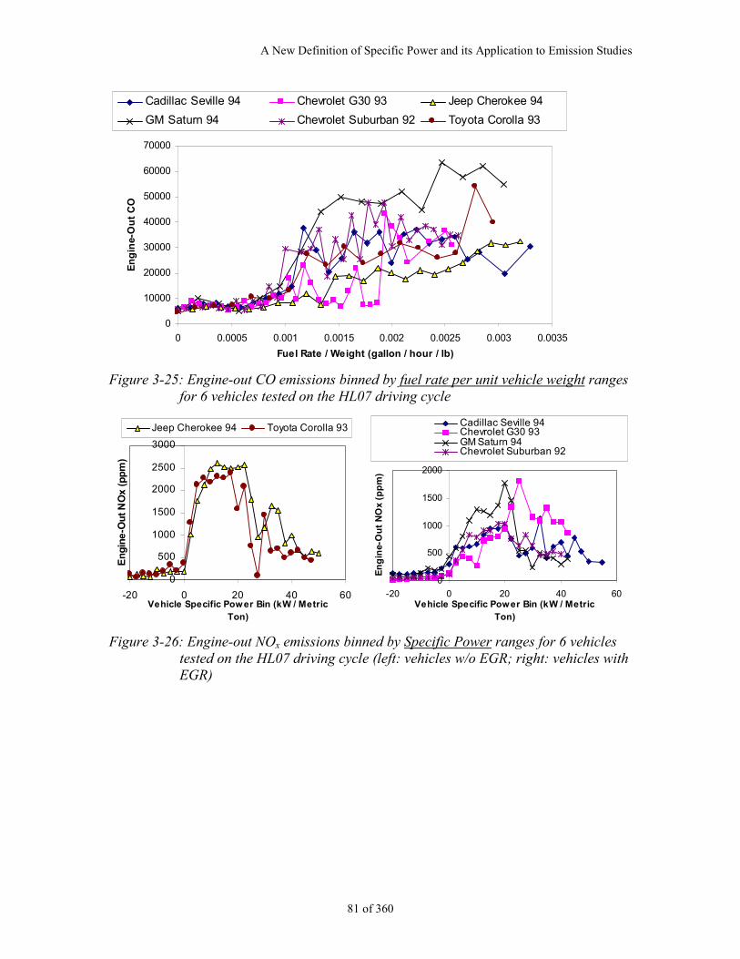
A New Definition of Specific Power and its Application to Emission Studies

81 of 360

0

10000

20000

30000

40000

50000

60000

70000

0 0.0005 0.001 0.0015 0.002 0.0025 0.003 0.0035

Fuel Rate / Weight (gallon / hour / lb)

En

gin

e-O

ut

CO

Cadillac Seville 94 Chevrolet G30 93 Jeep Cherokee 94

GM Saturn 94 Chevrolet Suburban 92 Toyota Corolla 93

Figure 3-25: Engine-out CO emissions binned by fuel rate per unit vehicle weight rangesfor 6 vehicles tested on the HL07 driving cycle

0

500

1000

1500

2000

2500

3000

-20 0 20 40 60Vehicle Specific Power Bin (kW / Metric

Ton)

En

gin

e-O

ut

NO

x (

pp

m)

Jeep Cherokee 94 Toyota Corolla 93

0

500

1000

1500

2000

-20 0 20 40 60Vehicle Specific Power Bin (kW / Metric

Ton)

En

gin

e-O

ut

NO

x (p

pm

)

Cadillac Seville 94Chevrolet G30 93GM Saturn 94Chevrolet Suburban 92

Figure 3-26: Engine-out NOx emissions binned by Specific Power ranges for 6 vehiclestested on the HL07 driving cycle (left: vehicles w/o EGR; right: vehicles withEGR)

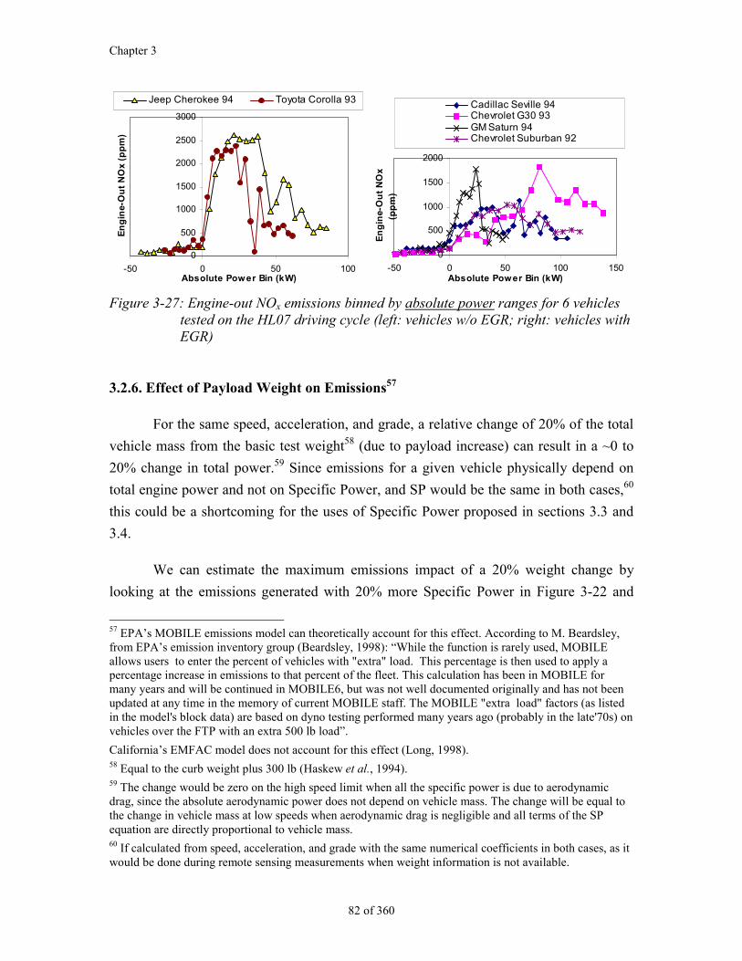
Chapter 3

82 of 360

0

500

1000

1500

2000

2500

3000

-50 0 50 100Absolute Power Bin (kW)

En

gin

e-O

ut

NO

x (p

pm

)

Jeep Cherokee 94 Toyota Corolla 93

0

500

1000

1500

2000

-50 0 50 100 150Absolute Power Bin (kW)

En

gin

e-O

ut

NO

x(p

pm

)

Cadillac Seville 94Chevrolet G30 93GM Saturn 94Chevrolet Suburban 92

Figure 3-27: Engine-out NOx emissions binned by absolute power ranges for 6 vehiclestested on the HL07 driving cycle (left: vehicles w/o EGR; right: vehicles withEGR)

3.2.6. Effect of Payload Weight on Emissions57

For the same speed, acceleration, and grade, a relative change of 20% of the total

vehicle mass from the basic test weight58 (due to payload increase) can result in a ~0 to

20% change in total power.59 Since emissions for a given vehicle physically depend on

total engine power and not on Specific Power, and SP would be the same in both cases,60

this could be a shortcoming for the uses of Specific Power proposed in sections 3.3 and

3.4.

We can estimate the maximum emissions impact of a 20% weight change by

looking at the emissions generated with 20% more Specific Power in Figure 3-22 and

57 EPA’s MOBILE emissions model can theoretically account for this effect. According to M. Beardsley,from EPA’s emission inventory group (Beardsley, 1998): “While the function is rarely used, MOBILEallows users to enter the percent of vehicles with "extra" load. This percentage is then used to apply apercentage increase in emissions to that percent of the fleet. This calculation has been in MOBILE formany years and will be continued in MOBILE6, but was not well documented originally and has not beenupdated at any time in the memory of current MOBILE staff. The MOBILE "extra load" factors (as listedin the model's block data) are based on dyno testing performed many years ago (probably in the late'70s) onvehicles over the FTP with an extra 500 lb load”.

California’s EMFAC model does not account for this effect (Long, 1998).58 Equal to the curb weight plus 300 lb (Haskew et al., 1994).59 The change would be zero on the high speed limit when all the specific power is due to aerodynamicdrag, since the absolute aerodynamic power does not depend on vehicle mass. The change will be equal tothe change in vehicle mass at low speeds when aerodynamic drag is negligible and all terms of the SPequation are directly proportional to vehicle mass.60 If calculated from speed, acceleration, and grade with the same numerical coefficients in both cases, as itwould be done during remote sensing measurements when weight information is not available.

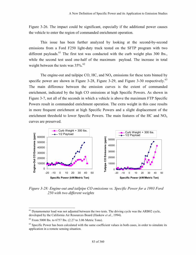
A New Definition of Specific Power and its Application to Emission Studies

83 of 360

Figure 3-26. The impact could be significant, especially if the additional power causes

the vehicle to enter the region of commanded enrichment operation.

This issue has been further analyzed by looking at the second-by-second

emissions from a Ford F250 light-duty truck tested on the SFTP program with two

different payloads.61 The first test was conducted with the curb weight plus 300 lbs.,

while the second test used one-half of the maximum payload. The increase in total

weight between the tests was 35%.62

The engine-out and tailpipe CO, HC, and NOx emissions for these tests binned by

specific power are shown in Figure 3-28, Figure 3-29, and Figure 3-30 respectively.63

The main difference between the emission curves is the extent of commanded

enrichment, indicated by the high CO emissions at high Specific Powers. As shown in

Figure 3-7, not all of the seconds in which a vehicle is above the maximum FTP Specific

Powers result in commanded enrichment operation. The extra weight in this case results

in more frequent enrichment at high Specific Powers and a slight displacement of the

enrichment threshold to lower Specific Powers. The main features of the HC and NOx

curves are preserved.

0

10000

20000

30000

40000

50000

60000

-20 -10 0 10 20 30 40 50

Specific Power (kW/Metric Ton)

En

gin

e-O

ut

CO

Em

iss

ion

s (

pp

m)

Curb Weight + 300 lbs.1/2 Payload

0

10000

20000

30000

40000

50000

-20 -10 0 10 20 30 40 50

Specific Power (kW/Metric Ton)

Ta

ilpip

e C

O E

mis

sio

ns

(p

pm

)

Curb Weight + 300 lbs.1/2 Payload

Figure 3-28: Engine-out and tailpipe CO emissions vs. Specific Power for a 1993 Ford250 with two different weights

61 Dynamometer load was not adjusted between the two tests. The driving cycle was the ARB02 cycle,developed by the California Air Resources Board (Haskew et al., 1994).62 From 5000 lbs. to 6757 lbs. (2.27 to 3.06 Metric Tons).63 Specific Power has been calculated with the same coefficient values in both cases, in order to simulate itsapplication in a remote sensing situation.

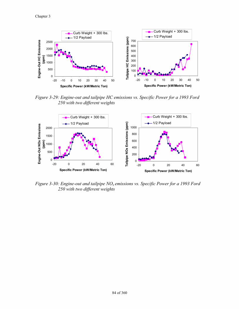
Chapter 3

84 of 360

0

500

1000

1500

2000

2500

-20 -10 0 10 20 30 40 50

Specific Power (kW/Metric Ton)

En

gin

e-O

ut

HC

Em

iss

ion

s(p

pm

)

Curb Weight + 300 lbs.1/2 Payload

0

100

200

300

400

500

600

700

-20 -10 0 10 20 30 40 50

Specific Power (kW/Metric Ton)

Ta

ilpip

e H

C E

mis

sio

ns

(p

pm

)

Curb Weight + 300 lbs.

1/2 Payload

Figure 3-29: Engine-out and tailpipe HC emissions vs. Specific Power for a 1993 Ford250 with two different weights

0

500

1000

1500

2000

-20 0 20 40 60

Specific Power (kW/Metric Ton)

En

gin

e-O

ut

NO

x E

mis

sio

ns

(pp

m)

Curb Weight + 300 lbs.

1/2 Payload

0

200

400

600

800

1000

-20 0 20 40 60

Specific Power (kW/Metric Ton)

Ta

ilpip

e N

Ox

Em

iss

ion

s (

pp

m)

Curb Weight + 300 lbs.

1/2 Payload

Figure 3-30: Engine-out and tailpipe NOx emissions vs. Specific Power for a 1993 Ford250 with two different weights

A New Definition of Specific Power and its Application to Emission Studies

85 of 360

3.3. Applications of Specific Power for Remote Sensing

3.3.1. Transient High Emissions and Remote Sensing

A potential application of remote sensing is as a “surveillance” component on

inspection and maintenance programs, either to detect high emitters and direct them to a

inspection and maintenance (I/M) programs, or to detect clean vehicles to exempt them

from I/M testing. The attempts to design and implement these programs in practice have

been hampered by the lack of a reliable method to screen out the occasional high

emissions of properly functioning vehicles, that would lead to “false failures.”64, 65 This is

the main reason why the U.S. EPA does not support the use of remote sensing to detect

high emitters (Lorang, 1998).

An adequate method to screen out these transient high emissions in remote

sensing measurements is needed. Some studies have tried to use speed and acceleration as

a way to screen out these conditions (Todd et al., 1995; Ripberger et al., 1996; Walsh et

al., 1998). However, the power needed from an engine to accelerate a vehicle is

influenced by the vehicle speed, the acceleration rate, and the roadway grade (see section

3.1). Thus, neither speed or acceleration, by itself, is a good measure of the load placed

on the engine. Two-dimensional regions on speed and acceleration can be used in

principle, but their determination and use is more complex, and a different map needs to

be used for each roadway grade. In the next sections the application of Specific Power to

this task is studied, based on the results of section 3.2.

Another remote sensing application is the evaluation of I/M programs (Zhang et al.,

1996b; Stedman et al., 1997b; Stedman et al., 1998). It could also benefit from a method to

screen out transient high emissions, since these are normally not encountered during I/M

testing.

Finally, a third use of remote sensing data is as in input in the calculation

emission inventories (Singer et al., 1996). In this case all of the data need to be taken into

64 “False failures” occur when a vehicle which would have emissions lower than the applicable standard onthe IM240 or FTP dynamometer tests is declared high emitter by a remote sensing surveillance program.“False passes” happen when a vehicle which would fail the dynamometer tests is declared a low emitter byremote sensing.65 Note that these transient high emissions captured by remote sensing are correct measurements of theactual emissions. They should be screened out because they are not indicative of a failure that could berepaired through an I/M program.

Chapter 3

86 of 360

account, since the transient high emissions are real and can account for a significant

fraction of the total emissions (An et al., 1997; Ross et al., 1998). A method to account

for the effect of the variation of driving conditions on the inventory is described in

section 3.4.2.

3.3.2. Analogies Between Second-by-Second Driving Cycle Data and Remote Sensing

Data

In the following sections some conclusions are made about remote sensing

measurements based on the results of second-by-second vehicle emission measurements

on driving cycles presented in section 3.2. This assumes that second-by-second data and

remote sensing measurements are analogous.

This analogy is clearly justified to the extent that dynamometer loads approximate

road loads, since individual remote sensing measurements sample the instantaneous

emissions with a time scale on the order of 0.5 seconds (see Figure 5-5).

For fleet averaged emissions, the rationale is the following: a second-by-second

dynamometer data set represents the emissions of a vehicle under a distribution of

operating conditions.66 If remote sensing measurements of the same vehicle were

performed, it is reasonable to assume that the range of emissions at each condition would

be similar. E.g. if the remote sensing emissions of the same vehicle were plotted vs.

Specific Power we would expect to have results such as those in Figure 3-7 for the

second-by-second emissions and similar to Figure 3-8 to Figure 3-14 for binned data.

Some preliminary evidence of this fact can be found by comparing the tailpipe CO

emission of Figure 3-7 with Figure 3-31, which show similar characteristics even though

they correspond to different vehicles..

Generalizing that idea, we can think of a given fleet67 measured by remote sensing

as a “composite vehicle,” which, given a sufficient number of measurements, will

produce stable curves of emissions vs. Specific Power such as those in Figure 3-8 to

Figure 3-14. These curves may then be used to predict emissions under different

conditions as described in section 3.3.6.

66 Again note that we are explicitly excluding cold-start operation. The discussion refers to hot stabilizedemissions only.67 Or subfleets such as 1990 light-duty trucks and TWC-equipped passenger cars.

A New Definition of Specific Power and its Application to Emission Studies

87 of 360

3.3.3. Criteria for Interpreting and Screening Remote Sensing Emission

Measurements

Variations in engine power demand are responsible for a significant part of the

variability encountered in remote sensing measurements. Specific Power can be used to

guide the interpretation and increase the usefulness of these measurements, by reducing

the occurrence of “false failures” and “false passes.”

Some rules for the interpretation of remote sensing measurements can be derived

from the analysis in section 3.2:

Vehicles with high CO emissions measured under Specific Powers beyond the FTP

maximum (~22 kW/Metric Ton) are suspect of commanded enrichment68 and should

be rejected. Those with high CO readings and Specific Powers below the FTP

maximum are likely to be real high emitters which are running with rich fuel-air

mixtures. A similar criterion was recently was recently proposed by McClintock

(1998). This criterion is a very effective way to screen out the high CO emissions

associated with commanded enrichment operation. It has the potential to greatly

reduce the associated erroneous high emitter identifications, as demonstrated in

section 3.3.5.

For example Walsh and Kite (Walsh et al., 1998) recently estimated that up to 65% of

the remotely sensed vehicles in their study with accelerations of 5-6 mph/sec were

high CO emitters, when it is likely that most of them were simply under commanded

enrichment.69

Specific Power could also be used to determine the threshold for commanded

enrichment for different vehicle models using large remote sensing data sets. This

information would be useful for representing the effect of enrichment on emission

models.

HC measurements associated with negative Specific Powers should be rejected as

well, since properly functioning vehicles may have high HC emission levels during

strong decelerations.70

68 See Figure 3-18 and Figure 3-21 in section 3.2.4.69 A vehicle with an acceleration of 5.5 mph/sec and a speed of 20 mph or larger will have an specificpower larger than the FTP maximum.70 See section 3.2.2.

Chapter 3

88 of 360

NOx measurements for negative Specific Powers should be rejected as well. Under

these conditions a vehicle with a broken catalyst may produce very low NOx

emissions71 due to low combustion temperatures. If load was not taken into account

such a vehicle would be considered a low-NOx emitter incorrectly .

Based on the limited data analyzed here, there is no reason to reject NOx

measurements at high Specific Powers or CO measurements at negative SPs.

Remote sensing measurements with high Specific Power (> 15 kW/Metric Ton), and

with both low CO (< 0.1%) and low NOx (< 100 ppm) are a very strong indication of

a properly functioning control system. The low CO emissions indicate that the

commanded enrichment strategy is not being used and that the vehicle is not running

rich for other reasons. Thus engine-out NOx emissions are necessarily high (see

Figure 3-7 and Figure 3-13). The low tailpipe concentrations of NOx and CO indicate

that the catalyst is being very effective for both pollutants. Vehicles with a remote

sensing measurement that fulfills this requirement could be exempted from I/M

testing for the current testing period without the need for a second measurement.72, 73

3.3.4. Verification of Commanded Enrichment Screening Using Specific Power

The criteria for commanded enrichment screening in remote sensing was verified

experimentally based on several remote sensing measurements of a vehicle which had

been recently verified to comply with the Ultra Low Emission Vehicle standards on the

FTP cycle.74 The CO emissions of this vehicle vs. Specific Power are shown in Figure

3-31. High CO emissions, indicating commanded enrichment, appear for Specific Power

values slightly above the maximum FTP values.75

This result indicates that the screening criterion is necessary: otherwise a remote

sensing program could classify this legally ultra-clean vehicle as a high CO emitter, if its

71 See section 3.2.2.72 Low HC emissions should also be required.73 This conclusion should be confirmed by analyzing a data set with remote sensing and IM240 data on thesame vehicles.74 This vehicle was made available to us during our measurement campaign at El Segundo, California (seeChapter 6) by an automobile manufacturer. The emission tests were performed by the California AirResources Board.75 NO emissions for this vehicle are shown in 5.4.2, and did not increase for the highest specific powers.HC emissions also stayed at very low levels for all powers (not shown).

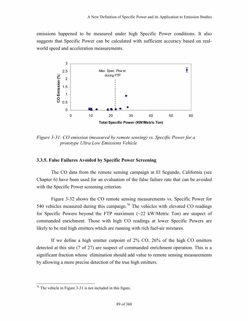
A New Definition of Specific Power and its Application to Emission Studies

89 of 360

emissions happened to be measured under high Specific Power conditions. It also

suggests that Specific Power can be calculated with sufficient accuracy based on real-

world speed and acceleration measurements.

0

0.5

1

1.5

2

2.5

3

0 10 20 30 40 50 60

Total Specific Power (KW/Metric Ton)

CO

Em

iss

ion

(%

)

Max. Spec. Pow erduring FTP

Figure 3-31: CO emission (measured by remote sensing) vs. Specific Power for aprototype Ultra Low Emissions Vehicle

3.3.5. False Failures Avoided by Specific Power Screening

The CO data from the remote sensing campaign at El Segundo, California (see

Chapter 6) have been used for an evaluation of the false failure rate that can be avoided

with the Specific Power screening criterion.

Figure 3-32 shows the CO remote sensing measurements vs. Specific Power for

540 vehicles measured during this campaign.76 The vehicles with elevated CO readings

for Specific Powers beyond the FTP maximum (~22 kW/Metric Ton) are suspect of

commanded enrichment. Those with high CO readings at lower Specific Powers are

likely to be real high emitters which are running with rich fuel-air mixtures.

If we define a high emitter cutpoint of 2% CO, 26% of the high CO emitters

detected at this site (7 of 27) are suspect of commanded enrichment operation. This is a

significant fraction whose elimination should add value to remote sensing measurements

by allowing a more precise detection of the true high emitters.

76 The vehicle in Figure 3-31 is not included in this figure.

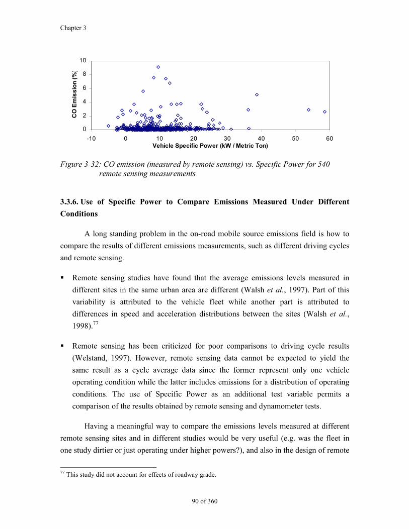
Chapter 3

90 of 360

0

2

4

6

8

10

-10 0 10 20 30 40 50 60Vehicle Specific Power (kW / Metric Ton)

CO

Em

iss

ion

(%

)

Figure 3-32: CO emission (measured by remote sensing) vs. Specific Power for 540remote sensing measurements

3.3.6. Use of Specific Power to Compare Emissions Measured Under Different

Conditions

A long standing problem in the on-road mobile source emissions field is how to

compare the results of different emissions measurements, such as different driving cycles

and remote sensing.

Remote sensing studies have found that the average emissions levels measured in

different sites in the same urban area are different (Walsh et al., 1997). Part of this

variability is attributed to the vehicle fleet while another part is attributed to

differences in speed and acceleration distributions between the sites (Walsh et al.,

1998).77

Remote sensing has been criticized for poor comparisons to driving cycle results

(Welstand, 1997). However, remote sensing data cannot be expected to yield the

same result as a cycle average data since the former represent only one vehicle

operating condition while the latter includes emissions for a distribution of operating

conditions. The use of Specific Power as an additional test variable permits a

comparison of the results obtained by remote sensing and dynamometer tests.

Having a meaningful way to compare the emissions levels measured at different

remote sensing sites and in different studies would be very useful (e.g. was the fleet in

one study dirtier or just operating under higher powers?), and also in the design of remote

77 This study did not account for effects of roadway grade.

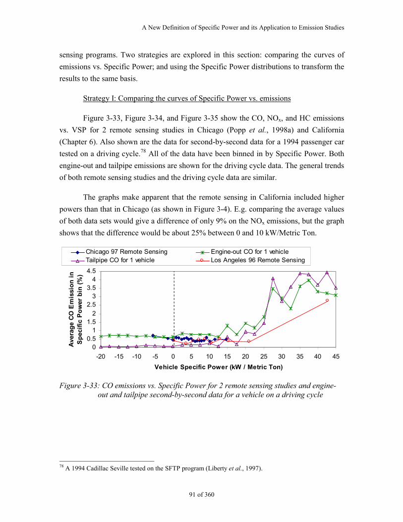
A New Definition of Specific Power and its Application to Emission Studies

91 of 360

sensing programs. Two strategies are explored in this section: comparing the curves of

emissions vs. Specific Power; and using the Specific Power distributions to transform the

results to the same basis.

Strategy I: Comparing the curves of Specific Power vs. emissions

Figure 3-33, Figure 3-34, and Figure 3-35 show the CO, NOx, and HC emissions

vs. VSP for 2 remote sensing studies in Chicago (Popp et al., 1998a) and California

(Chapter 6). Also shown are the data for second-by-second data for a 1994 passenger car

tested on a driving cycle.78 All of the data have been binned in by Specific Power. Both

engine-out and tailpipe emissions are shown for the driving cycle data. The general trends

of both remote sensing studies and the driving cycle data are similar.

The graphs make apparent that the remote sensing in California included higher

powers than that in Chicago (as shown in Figure 3-4). E.g. comparing the average values

of both data sets would give a difference of only 9% on the NOx emissions, but the graph

shows that the difference would be about 25% between 0 and 10 kW/Metric Ton.

00.5

11.5

2

2.53

3.54

4.5

-20 -15 -10 -5 0 5 10 15 20 25 30 35 40 45

Vehicle Specific Power (kW / Metric Ton)

Ave

rag

e C

O E

mis

sio

n i

n

Sp

ecif

ic P

ow

er b

in (

%)

Chicago 97 Remote Sensing Engine-out CO for 1 vehicleTailpipe CO for 1 vehicle Los Angeles 96 Remote Sensing

Figure 3-33: CO emissions vs. Specific Power for 2 remote sensing studies and engine-out and tailpipe second-by-second data for a vehicle on a driving cycle

78 A 1994 Cadillac Seville tested on the SFTP program (Liberty et al., 1997).

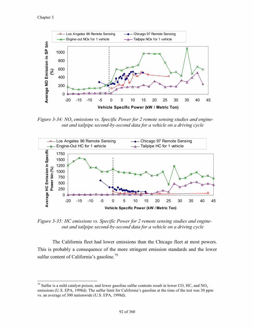
Chapter 3

92 of 360

0

200

400

600

800

1000

-20 -15 -10 -5 0 5 10 15 20 25 30 35 40 45

Vehicle Specific Power (kW / Metric Ton)

Ave

rag

e N

O E

mis

sio

n i

n S

P b

in

(%)

Los Angeles 96 Remote Sensing Chicago 97 Remote Sensing

Engine-out NOx for 1 vehicle Tailpipe NOx for 1 vehicle

Figure 3-34: NOx emissions vs. Specific Power for 2 remote sensing studies and engine-out and tailpipe second-by-second data for a vehicle on a driving cycle

0

250

500

750

1000

1250

1500

1750

-20 -15 -10 -5 0 5 10 15 20 25 30 35 40 45

Vehicle Specific Power (kW / Metric Ton)Av

era

ge

HC

Em

iss

ion

in S

pe

cif

icP

ow

er

bin

(%

)

Los Angeles 96 Remote Sensing Chicago 97 Remote SensingEngine-Out HC for 1 vehicle Tailpipe HC for 1 vehicle

Figure 3-35: HC emissions vs. Specific Power for 2 remote sensing studies and engine-out and tailpipe second-by-second data for a vehicle on a driving cycle

The California fleet had lower emissions than the Chicago fleet at most powers.

This is probably a consequence of the more stringent emission standards and the lower

sulfur content of California’s gasoline.79

79 Sulfur is a mild catalyst poison, and lower gasoline sulfur contents result in lower CO, HC, and NOx

emissions (U.S. EPA, 1998d). The sulfur limit for California’s gasoline at the time of the test was 30 ppmvs. an average of 300 nationwide (U.S. EPA, 1998d).

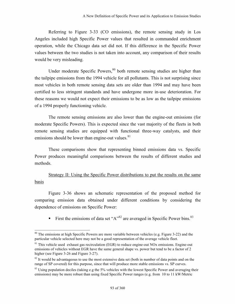
A New Definition of Specific Power and its Application to Emission Studies

93 of 360

Referring to Figure 3-33 (CO emissions), the remote sensing study in Los

Angeles included high Specific Power values that resulted in commanded enrichment

operation, while the Chicago data set did not. If this difference in the Specific Power

values between the two studies is not taken into account, any comparison of their results

would be very misleading.

Under moderate Specific Powers,80 both remote sensing studies are higher than

the tailpipe emissions from the 1994 vehicle for all pollutants. This is not surprising since

most vehicles in both remote sensing data sets are older than 1994 and may have been

certified to less stringent standards and have undergone more in-use deterioration. For

these reasons we would not expect their emissions to be as low as the tailpipe emissions

of a 1994 properly functioning vehicle.

The remote sensing emissions are also lower than the engine-out emissions (for

moderate Specific Powers). This is expected since the vast majority of the fleets in both

remote sensing studies are equipped with functional three-way catalysts, and their

emissions should be lower than engine-out values.81

These comparisons show that representing binned emissions data vs. Specific

Power produces meaningful comparisons between the results of different studies and

methods.

Strategy II: Using the Specific Power distributions to put the results on the same

basis

Figure 3-36 shows an schematic representation of the proposed method for

comparing emission data obtained under different conditions by considering the

dependence of emissions on Specific Power:

First the emissions of data set “A”82 are averaged in Specific Power bins.83

80 The emissions at high Specific Powers are more variable between vehicles (e.g. Figure 3-22) and theparticular vehicle selected here may not be a good representation of the average vehicle fleet.81 This vehicle used exhaust gas recirculation (EGR) to reduce engine-out NOx emissions. Engine-outemissions of vehicles without EGR have the same general shape vs. power but tend to be a factor of 2higher (see Figure 3-26 and Figure 3-27).82 It would be advantageous to use the most extensive data set (both in number of data points and on therange of SP covered) for this purpose, since that will produce more stable emissions vs. SP curves.83 Using population deciles (taking e.g the 5% vehicles with the lowest Specific Power and averaging theiremissions) may be more robust than using fixed Specific Power ranges (e.g. from 10 to 11 kW/Metric

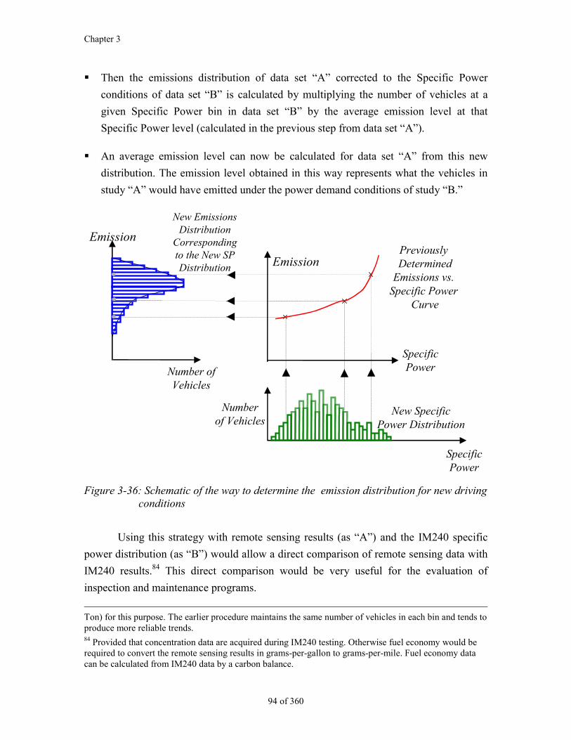
Chapter 3

94 of 360

Then the emissions distribution of data set “A” corrected to the Specific Power

conditions of data set “B” is calculated by multiplying the number of vehicles at a

given Specific Power bin in data set “B” by the average emission level at that

Specific Power level (calculated in the previous step from data set “A”).

An average emission level can now be calculated for data set “A” from this new

distribution. The emission level obtained in this way represents what the vehicles in

study “A” would have emitted under the power demand conditions of study “B.”

SpecificPower

New EmissionsDistribution

Correspondingto the New SPDistribution

Previously Determined

Emissions vs. Specific Power

Curve

Emission

New SpecificPower Distribution

SpecificPower

Numberof Vehicles

Number ofVehicles

Emission

Figure 3-36: Schematic of the way to determine the emission distribution for new drivingconditions

Using this strategy with remote sensing results (as “A”) and the IM240 specific

power distribution (as “B”) would allow a direct comparison of remote sensing data with

IM240 results.84 This direct comparison would be very useful for the evaluation of

inspection and maintenance programs.

Ton) for this purpose. The earlier procedure maintains the same number of vehicles in each bin and tends toproduce more reliable trends.84 Provided that concentration data are acquired during IM240 testing. Otherwise fuel economy would berequired to convert the remote sensing results in grams-per-gallon to grams-per-mile. Fuel economy datacan be calculated from IM240 data by a carbon balance.

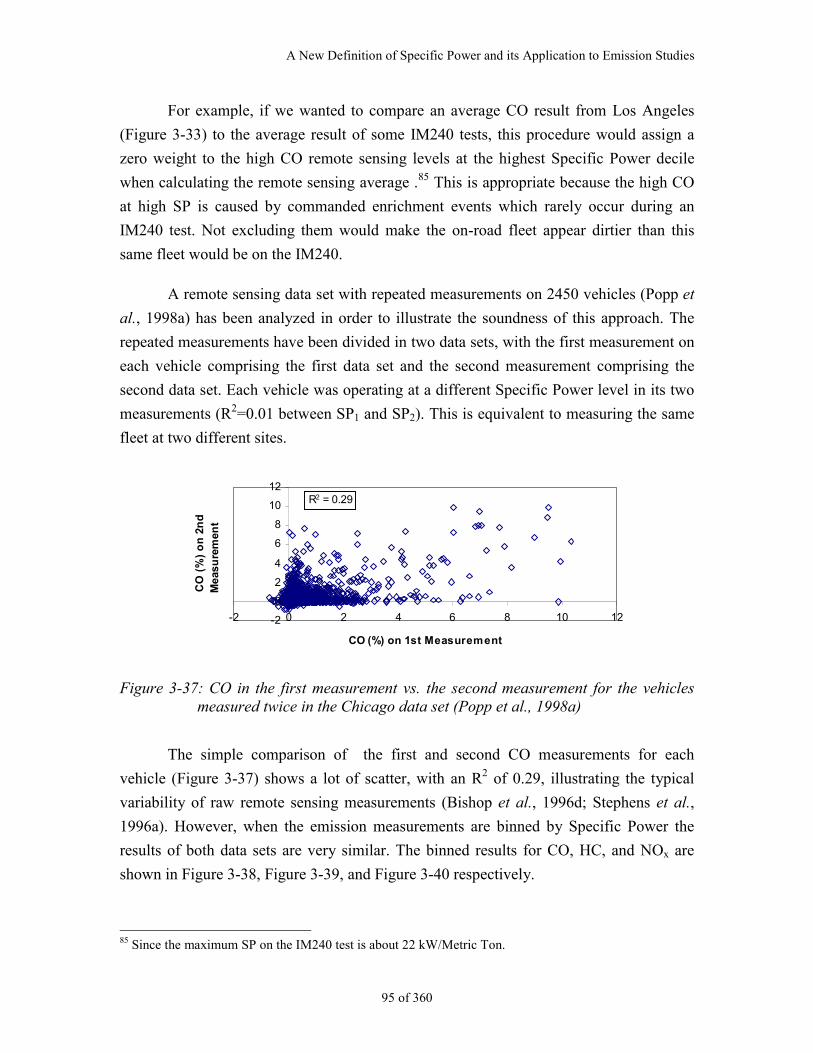
A New Definition of Specific Power and its Application to Emission Studies

95 of 360

For example, if we wanted to compare an average CO result from Los Angeles

(Figure 3-33) to the average result of some IM240 tests, this procedure would assign a

zero weight to the high CO remote sensing levels at the highest Specific Power decile

when calculating the remote sensing average .85 This is appropriate because the high CO

at high SP is caused by commanded enrichment events which rarely occur during an

IM240 test. Not excluding them would make the on-road fleet appear dirtier than this

same fleet would be on the IM240.

A remote sensing data set with repeated measurements on 2450 vehicles (Popp et

al., 1998a) has been analyzed in order to illustrate the soundness of this approach. The

repeated measurements have been divided in two data sets, with the first measurement on

each vehicle comprising the first data set and the second measurement comprising the

second data set. Each vehicle was operating at a different Specific Power level in its two

measurements (R2=0.01 between SP1 and SP2). This is equivalent to measuring the same

fleet at two different sites.

-2

0

2

4

6

8

10

12

-2 0 2 4 6 8 10 12

CO (%) on 1st Measurement

CO

(%

) o

n 2

nd

M

easu

rem

ent

R2 = 0.29

Figure 3-37: CO in the first measurement vs. the second measurement for the vehiclesmeasured twice in the Chicago data set (Popp et al., 1998a)

The simple comparison of the first and second CO measurements for each

vehicle (Figure 3-37) shows a lot of scatter, with an R2 of 0.29, illustrating the typical

variability of raw remote sensing measurements (Bishop et al., 1996d; Stephens et al.,

1996a). However, when the emission measurements are binned by Specific Power the

results of both data sets are very similar. The binned results for CO, HC, and NOx are

shown in Figure 3-38, Figure 3-39, and Figure 3-40 respectively.

85 Since the maximum SP on the IM240 test is about 22 kW/Metric Ton.

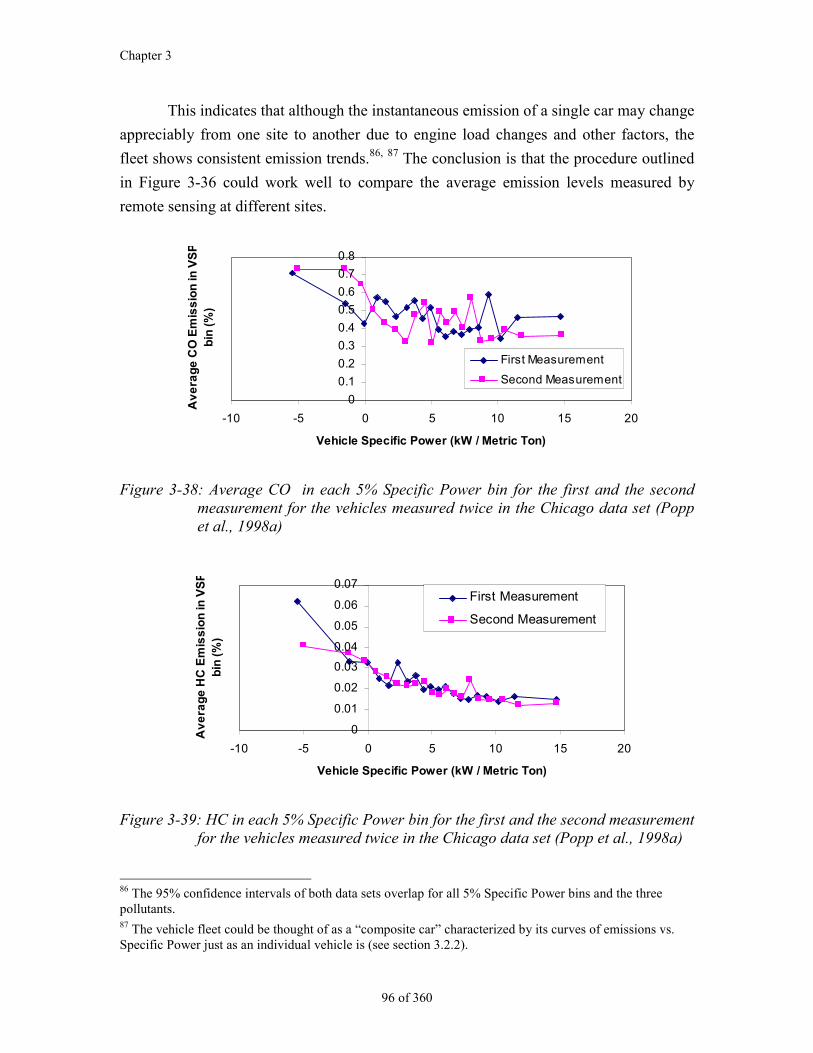
Chapter 3

96 of 360

This indicates that although the instantaneous emission of a single car may change

appreciably from one site to another due to engine load changes and other factors, the

fleet shows consistent emission trends.86, 87 The conclusion is that the procedure outlined

in Figure 3-36 could work well to compare the average emission levels measured by

remote sensing at different sites.

0

0.1

0.2

0.3

0.4

0.5

0.6

0.7

0.8

-10 -5 0 5 10 15 20

Vehicle Specific Power (kW / Metric Ton)

Av

era

ge

CO

Em

iss

ion

in V

SP

bin

(%

)

First Measurement

Second Measurement

Figure 3-38: Average CO in each 5% Specific Power bin for the first and the secondmeasurement for the vehicles measured twice in the Chicago data set (Poppet al., 1998a)

0

0.01

0.02

0.03

0.04

0.05

0.06

0.07

-10 -5 0 5 10 15 20

Vehicle Specific Power (kW / Metric Ton)

Av

era

ge

HC

Em

iss

ion

in V

SP

bin

(%

)

First Measurement

Second Measurement

Figure 3-39: HC in each 5% Specific Power bin for the first and the second measurementfor the vehicles measured twice in the Chicago data set (Popp et al., 1998a)

86 The 95% confidence intervals of both data sets overlap for all 5% Specific Power bins and the threepollutants.87 The vehicle fleet could be thought of as a “composite car” characterized by its curves of emissions vs.Specific Power just as an individual vehicle is (see section 3.2.2).

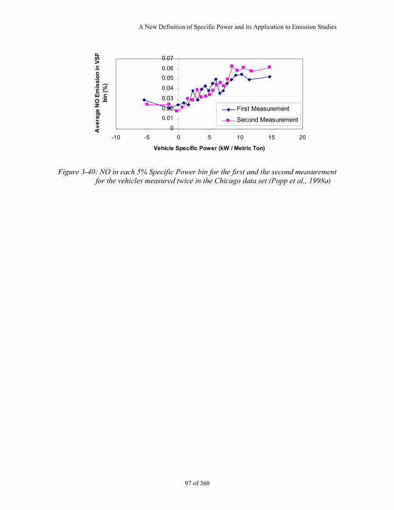
A New Definition of Specific Power and its Application to Emission Studies

97 of 360

0

0.01

0.02

0.03

0.04

0.05

0.06

0.07

-10 -5 0 5 10 15 20

Vehicle Specific Power (kW / Metric Ton)

Av

era

ge

NO

Em

iss

ion

in V

SP

bin

(%

)First Measurement

Second Measurement

Figure 3-40: NO in each 5% Specific Power bin for the first and the second measurementfor the vehicles measured twice in the Chicago data set (Popp et al., 1998a)

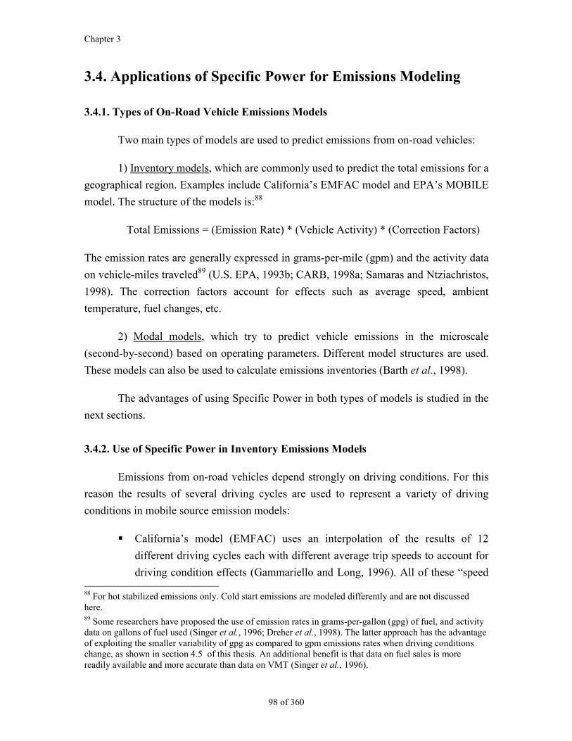
Chapter 3

98 of 360

3.4. Applications of Specific Power for Emissions Modeling

3.4.1. Types of On-Road Vehicle Emissions Models

Two main types of models are used to predict emissions from on-road vehicles:

1) Inventory models, which are commonly used to predict the total emissions for a

geographical region. Examples include California’s EMFAC model and EPA’s MOBILE

model. The structure of the models is:88

Total Emissions = (Emission Rate) * (Vehicle Activity) * (Correction Factors)

The emission rates are generally expressed in grams-per-mile (gpm) and the activity data

on vehicle-miles traveled89 (U.S. EPA, 1993b; CARB, 1998a; Samaras and Ntziachristos,

1998). The correction factors account for effects such as average speed, ambient

temperature, fuel changes, etc.

2) Modal models, which try to predict vehicle emissions in the microscale

(second-by-second) based on operating parameters. Different model structures are used.

These models can also be used to calculate emissions inventories (Barth et al., 1998).

The advantages of using Specific Power in both types of models is studied in the

next sections.

3.4.2. Use of Specific Power in Inventory Emissions Models

Emissions from on-road vehicles depend strongly on driving conditions. For this

reason the results of several driving cycles are used to represent a variety of driving

conditions in mobile source emission models:

California’s model (EMFAC) uses an interpolation of the results of 12

different driving cycles each with different average trip speeds to account for

driving condition effects (Gammariello and Long, 1996). All of these “speed 88 For hot stabilized emissions only. Cold start emissions are modeled differently and are not discussedhere.89 Some researchers have proposed the use of emission rates in grams-per-gallon (gpg) of fuel, and activitydata on gallons of fuel used (Singer et al., 1996; Dreher et al., 1998). The latter approach has the advantageof exploiting the smaller variability of gpg as compared to gpm emissions rates when driving conditionschange, as shown in section 4.5 of this thesis. An additional benefit is that data on fuel sales is morereadily available and more accurate than data on VMT (Singer et al., 1996).

A New Definition of Specific Power and its Application to Emission Studies

99 of 360

correction driving cycles” begin and end at idle, and the emissions of each

cycle are more indicative of trips of certain average speed90 than of emissions

associated with instantaneous speed. A regression analysis of the results from

the different cycles provides “speed correction factors,” which are then

applied to the basic vehicle emission rates to account for the variation of

driving conditions. The speed correction factors used by the EMFAC model

are shown in Figure 3-41 (CARB, 1998a).

0.0

0.5

1.0

1.5

2.0

2.5

3.0

3.5

0 10 20 30 40 50 60 70

Average Cycle Speed (mph)

Sp

ee

d C

orr

ec

tio

n F

ac

tor

CO

HC

NOx

Figure 3-41: EMFAC speed correction factors vs. average cycle speed for the regulatedpollutants

EPA’s model (MOBILE) uses the same approach (U.S. EPA, 1993b). The

version currently under development (MOBILE6) will make use of several

new “speed correction cycles.” These cycles are chosen based on matching the

joint distribution of speed and acceleration obtained from instrumented

vehicle and “chase car” data (Carlson et al., 1997).

Current European inventory emissions models also use the same approach as

EPA and CARB (Samaras et al., 1998).

Using average trip speed to represent different driving conditions has an

important limitation: trips with the same average speed may correspond to very different

Specific Power distributions and emissions. For example a trip in which half of the time

the vehicle is traveling at 60 mph and half is stopped would be assigned the same

emission rates than a trip at a constant 30 mph speed.

90 Defined as the distance traveled divided by the time spent in the driving cycle, including any stoppedtime.

Chapter 3

100 of 360

It is suggested here that a better way to model the dependence of emissions on

driving conditions would be to use correction factors based on distributions of Specific

Power. This would also permit a seamless integration of the effect of grade on emissions.

The suggested procedure for implementing this correction is as follows:

1) The dependence of emissions vs. Specific Power can be determined from

remote sensing and/or driving cycle data (e.g. Figure 3-14 and Figure 3-22 for

driving cycles; Figure 3-38 for remote sensing).

2) The distribution of Specific Powers in the geographical area and roadway type

of interest area can be obtained from instrumented vehicle and “chase car”

studies (Carlson et al., 1997).

3) Then the procedure outlined in Figure 3-36 can be used to relate the emissions

measured on a given driving cycle or remote sensing site to the emissions that

the fleet would produce with the measured distribution of Specific Powers.

3.4.3. Use of Specific Power in Modal Emissions Modeling

Modal emissions models attempt to predict the instantaneous vehicle emissions as

a function of operating parameters.

Many different input variables have been used in them. Some of these models

relate emissions directly to the joint distribution of speed and acceleration (Guensler et

al., 1997; West and McGill, 1997; Sturm et al., 1998). Other modal models use diverse

parameters non measurable from the roadside as surrogates for engine load. Examples

include:

Manifold vacuum and brake mean effective pressure (Koupal and German,

1995).

Mass air flow, estimated from the total power and gear switch points

(Ripberger et al., 1998).

Throttle position (Shih et al., 1997).

Fraction of available power being used (Guensler et al., 1997).

Fuel rate and the product of speed and acceleration (An et al., 1997).

A New Definition of Specific Power and its Application to Emission Studies

101 of 360

Speed and the product of speed and acceleration (Sturm et al., 1998).

Fuel Rate. The most comprehensive physics-based modal emission model

available, developed by the group at CE-CERT in U.C. Riverside, uses this

parameter as the basis for emissions modeling (Barth et al., 1997; Barth et al.,

1998; Nam et al., 1998).

Some very promising recent modal models are based on neural networks (Long et

al., 1997; Atkinson et al., 1998; Jesion et al., 1998). The network is given a time series of

a set of variables on a driving cycle and is then predicts what the emissions will be when

given a new set of input variables. The input variables used so far include vehicle speed,

engine speed, engine torque, and engine power demand.

Using Specific Powers instead of these diverse parameters cited above has two

main two advantages: Specific Power is directly measurable in real-world conditions, and

the dependence of emissions on SP is better than on the other measurable parameters (as

discussed in sections 3.2.4 and 3.2.4).

Neural network-based models could also benefit from the benefits of Specific

Power by using this parameter as an input variable. Models that use speed and

acceleration as inputs would be simplified by using only 1 parameter instead of 2.

Finally, those models that use non-measurable variables would benefit from switching to

a variable with a strong correlation with emissions but which is directly measurable in the

real world.

As mentioned above, it is not suggested here that instantaneous vehicle emissions

are only a “state” function of Specific Power. For example commanded enrichment may

or may not be used at the same Specific Power level (see Figure 3-7), and history effects

over several seconds may be important for the engine and the catalyst (An et al., 1997;

Nam et al., 1998). Rather the conclusion of this study is that instantaneous SP should be

used as the main variable representing engine load, although the history of SP or other

additional input variables may be needed to properly model all situations.

Chapter 3

102 of 360

3.5. Conclusions

The main results of the study in this chapter are:

Specific Power (SP), defined as the total tractive power per unit weight for a given

vehicle, can be calculated with good approximation from measurements of vehicle

speed, acceleration, and roadway grade and estimates of aerodynamic and rolling

resistance.

Emissions have a strong dependence on Specific Power. In particular Specific Power

is the best predictor of commanded enrichment in recent production vehicles, which

start to enrich at Specific Powers slightly above the maximum value of this parameter

on the FTP driving cycle.

Once Specific Power is known, speed and acceleration do not provide additional

information with respect to emissions.

Specific Power distributions or curves of emissions vs. Specific Power can be used to

relate the emissions produced on different driving cycles or at different remote

sensing sites.

The Specific Power that is relevant for remote sensing is that of the instant in which

the emissions which are leaving the tailpipe were generated in the engine. This means

that the speed and acceleration measurements should be done between 5 and 20

meters before the point where emissions are measured (for positive SPs).

Specific Power can be used to screen out remote sensing measurements under

conditions that lead to transient high emissions in properly functioning vehicles, since

these emissions may not be repairable through an inspection and maintenance

program. These include high CO and HC emissions due to commanded enrichment

and high HC emissions during strong or prolonged decelerations. Emissions

inventories should not screen out these high readings since they are correct

measurements of real phenomena that must be accounted for in an inventory.

Specific Power could be used to determine the threshold for commanded enrichment

for different vehicle models using large remote sensing data sets.

A New Definition of Specific Power and its Application to Emission Studies

103 of 360

Low NOx emissions in remote sensing situations when the vehicle is under very low

or negative Specific Power should also be screened out for I/M purposes. Under these

conditions a vehicle with a broken catalyst would have very low tailpipe NOx

emissions due to low NOx production in the engine.

Low NOx, CO, and HC in a remote sensing measurement under high Specific Power

is a strong indication that the emission control system of the vehicle is working

properly.

Emissions models can benefit from using Specific Power as the main parameter to

represent load since this parameter has a strong relationship with emissions and is

directly measurable in the real world.

- Inventory emissions models can benefit from the use of Specific Power-based

correction factors instead of speed-correction factors to represent the effect of

different driving conditions on warmed-up emissions.

- Modal emissions models can also be improved and/or simplified by using

Specific Power as the main load surrogate, in order to take advantage of the

good relationship between SP and emissions.

An additional benefit of the use of Specific Power in the different sub-fields would be

the use of a common parameter to represent load on emission studies performed with

different methods, such as dynamometers tests, remote sensing, and emissions

models. Such “common language” would allow a much easier and more detailed

comparison of the results of the different methods.

The main limitation of the new definition of Specific Power presented here is that it

cannot account for the emission impact of large increases in vehicle weight due to

payload, and of non-tractive power use such as for air conditioning operation. Some

strategies to deal with these problems are suggested. Further research is needed in

these areas.

105 of 360

Chapter 4. Analysis of Remote SensingMeasurements

4.1. Introduction

Remote sensing of on-road vehicle emissions was pioneered by Don Stedman and

Gary Bishop of the University of Denver in 1987 (Bishop et al., 1989). Since then several

other groups and companies have developed and used remote sensing instruments, and

remote sensing measurements have been made for millions of vehicles. However, some

basic aspects of the measurements have not been studied or documented.

This chapter presents analyses of a number of practical issues associated with

remote sensing measurements. These are of general applicability and are not restricted to

remote sensing with the TILDAS technique. Section 4.2 deals with the fluid mechanical

aspects of remote sensing measurements, including the interference between the exhaust

of two vehicles measured sequentially. Section 4.3 introduces the concept of plume

capture and some models and experimental data for its quantification. Section 4.4

analyzes the variation of remote sensing noise with plume capture and emission level.

Section 4.5 introduces the issues associated with the residence time of the exhaust gases

in the vehicle, and presents a model for its quantification. Section 4.6 shows the

advantage of using grams-per-gallon emission factors because of their lower variability

as compared to grams-per-mile emissions factors. The need to include the relative fuel

economy when using remote sensing data to compile emission inventories is

demonstrated in section 4.7. Finally section 4.8 summarizes the conclusions of this

chapter.

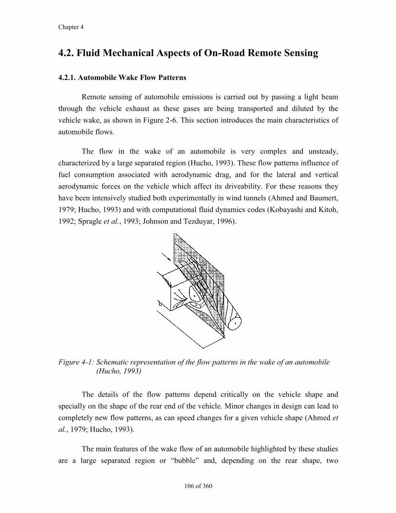
Chapter 4

106 of 360

4.2. Fluid Mechanical Aspects of On-Road Remote Sensing

4.2.1. Automobile Wake Flow Patterns

Remote sensing of automobile emissions is carried out by passing a light beam

through the vehicle exhaust as these gases are being transported and diluted by the

vehicle wake, as shown in Figure 2-6. This section introduces the main characteristics of

automobile flows.

The flow in the wake of an automobile is very complex and unsteady,

characterized by a large separated region (Hucho, 1993). These flow patterns influence of

fuel consumption associated with aerodynamic drag, and for the lateral and vertical

aerodynamic forces on the vehicle which affect its driveability. For these reasons they

have been intensively studied both experimentally in wind tunnels (Ahmed and Baumert,

1979; Hucho, 1993) and with computational fluid dynamics codes (Kobayashi and Kitoh,

1992; Spragle et al., 1993; Johnson and Tezduyar, 1996).

Figure 4-1: Schematic representation of the flow patterns in the wake of an automobile(Hucho, 1993)

The details of the flow patterns depend critically on the vehicle shape and

specially on the shape of the rear end of the vehicle. Minor changes in design can lead to

completely new flow patterns, as can speed changes for a given vehicle shape (Ahmed et

al., 1979; Hucho, 1993).

The main features of the wake flow of an automobile highlighted by these studies

are a large separated region or “bubble” and, depending on the rear shape, two

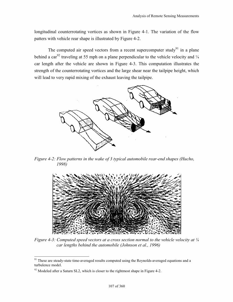
Analysis of Remote Sensing Measurements

107 of 360

longitudinal counterrotating vortices as shown in Figure 4-1. The variation of the flow

patters with vehicle rear shape is illustrated by Figure 4-2.

The computed air speed vectors from a recent supercomputer study91 in a plane

behind a car92 traveling at 55 mph on a plane perpendicular to the vehicle velocity and ¼

car length after the vehicle are shown in Figure 4-3. This computation illustrates the

strength of the counterrotating vortices and the large shear near the tailpipe height, which

will lead to very rapid mixing of the exhaust leaving the tailpipe.

Figure 4-2: Flow patterns in the wake of 3 typical automobile rear-end shapes (Hucho,1998)

Figure 4-3: Computed speed vectors at a cross section normal to the vehicle velocity at ¼car lengths behind the automobile (Johnson et al., 1996)

91 These are steady-state time-averaged results computed using the Reynolds-averaged equations and aturbulence model.92 Modeled after a Saturn SL2, which is closer to the rightmost shape in Figure 4-2.

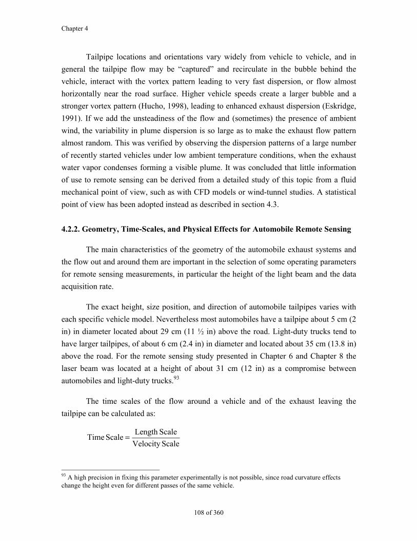
Chapter 4

108 of 360

Tailpipe locations and orientations vary widely from vehicle to vehicle, and in

general the tailpipe flow may be “captured” and recirculate in the bubble behind the

vehicle, interact with the vortex pattern leading to very fast dispersion, or flow almost

horizontally near the road surface. Higher vehicle speeds create a larger bubble and a

stronger vortex pattern (Hucho, 1998), leading to enhanced exhaust dispersion (Eskridge,

1991). If we add the unsteadiness of the flow and (sometimes) the presence of ambient

wind, the variability in plume dispersion is so large as to make the exhaust flow pattern

almost random. This was verified by observing the dispersion patterns of a large number

of recently started vehicles under low ambient temperature conditions, when the exhaust

water vapor condenses forming a visible plume. It was concluded that little information

of use to remote sensing can be derived from a detailed study of this topic from a fluid

mechanical point of view, such as with CFD models or wind-tunnel studies. A statistical

point of view has been adopted instead as described in section 4.3.

4.2.2. Geometry, Time-Scales, and Physical Effects for Automobile Remote Sensing

The main characteristics of the geometry of the automobile exhaust systems and

the flow out and around them are important in the selection of some operating parameters

for remote sensing measurements, in particular the height of the light beam and the data

acquisition rate.

The exact height, size position, and direction of automobile tailpipes varies with

each specific vehicle model. Nevertheless most automobiles have a tailpipe about 5 cm (2

in) in diameter located about 29 cm (11 ½ in) above the road. Light-duty trucks tend to

have larger tailpipes, of about 6 cm (2.4 in) in diameter and located about 35 cm (13.8 in)

above the road. For the remote sensing study presented in Chapter 6 and Chapter 8 the

laser beam was located at a height of about 31 cm (12 in) as a compromise between

automobiles and light-duty trucks.93

The time scales of the flow around a vehicle and of the exhaust leaving the

tailpipe can be calculated as:

Scale Velocity

Scale LengthScale Time =

93 A high precision in fixing this parameter experimentally is not possible, since road curvature effectschange the height even for different passes of the same vehicle.

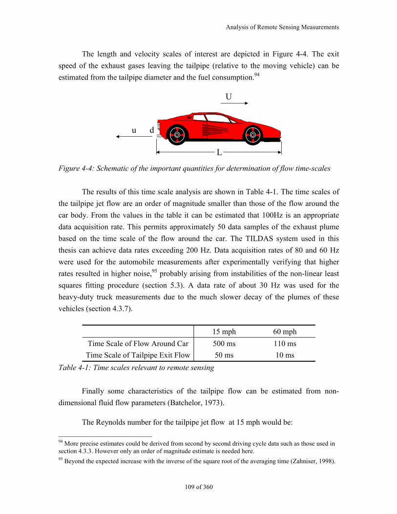
Analysis of Remote Sensing Measurements

109 of 360

The length and velocity scales of interest are depicted in Figure 4-4. The exit

speed of the exhaust gases leaving the tailpipe (relative to the moving vehicle) can be

estimated from the tailpipe diameter and the fuel consumption.94

U

u d

L

Figure 4-4: Schematic of the important quantities for determination of flow time-scales

The results of this time scale analysis are shown in Table 4-1. The time scales of

the tailpipe jet flow are an order of magnitude smaller than those of the flow around the

car body. From the values in the table it can be estimated that 100Hz is an appropriate

data acquisition rate. This permits approximately 50 data samples of the exhaust plume

based on the time scale of the flow around the car. The TILDAS system used in this

thesis can achieve data rates exceeding 200 Hz. Data acquisition rates of 80 and 60 Hz

were used for the automobile measurements after experimentally verifying that higher

rates resulted in higher noise,95 probably arising from instabilities of the non-linear least

squares fitting procedure (section 5.3). A data rate of about 30 Hz was used for the

heavy-duty truck measurements due to the much slower decay of the plumes of these

vehicles (section 4.3.7).

15 mph 60 mph

Time Scale of Flow Around Car 500 ms 110 ms

Time Scale of Tailpipe Exit Flow 50 ms 10 ms

Table 4-1: Time scales relevant to remote sensing

Finally some characteristics of the tailpipe flow can be estimated from non-

dimensional fluid flow parameters (Batchelor, 1973).

The Reynolds number for the tailpipe jet flow at 15 mph would be:

94 More precise estimates could be derived from second by second driving cycle data such as those used insection 4.3.3. However only an order of magnitude estimate is needed here.95 Beyond the expected increase with the inverse of the square root of the averaging time (Zahniser, 1998).

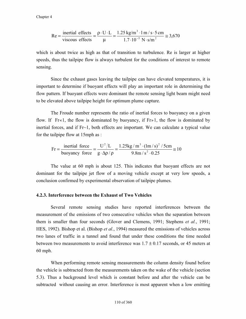
Chapter 4

110 of 360

670,3s/mN 107.1

cm 5s/m 1kg/m 25.1LU

effects viscous

ffectse inertialRe

25

3

≅⋅⋅

⋅⋅=

µ⋅⋅ρ==

−

which is about twice as high as that of transition to turbulence. Re is larger at higher

speeds, thus the tailpipe flow is always turbulent for the conditions of interest to remote

sensing.

Since the exhaust gases leaving the tailpipe can have elevated temperatures, it is

important to determine if buoyant effects will play an important role in determining the

flow pattern. If buoyant effects were dominant the remote sensing light beam might need

to be elevated above tailpipe height for optimum plume capture.

The Froude number represents the ratio of inertial forces to buoyancy on a given

flow. If Fr«1, the flow is dominated by buoyancy, if Fr»1, the flow is dominated by

inertial forces, and if Fr~1, both effects are important. We can calculate a typical value

for the tailpipe flow at 15mph as :

1025.0s/m8.9

cm5/)s/m1(m/kg25.1

/g

LU

force buoyancy

force linertiaFr

2

232

≅⋅

⋅=ρρ∆⋅

==

The value at 60 mph is about 125. This indicates that buoyant effects are not

dominant for the tailpipe jet flow of a moving vehicle except at very low speeds, a

conclusion confirmed by experimental observation of tailpipe plumes.

4.2.3. Interference between the Exhaust of Two Vehicles

Several remote sensing studies have reported interferences between the

measurement of the emissions of two consecutive vehicles when the separation between

them is smaller than four seconds (Glover and Clemens, 1991; Stephens et al., 1991;

HES, 1992). Bishop et al. (Bishop et al., 1994) measured the emissions of vehicles across

two lanes of traffic in a tunnel and found that under these conditions the time needed

between two measurements to avoid interference was 1.7 ± 0.17 seconds, or 45 meters at

60 mph.

When performing remote sensing measurements the column density found before

the vehicle is subtracted from the measurements taken on the wake of the vehicle (section

5.3). Thus a background level which is constant before and after the vehicle can be

subtracted without causing an error. Interference is most apparent when a low emitting

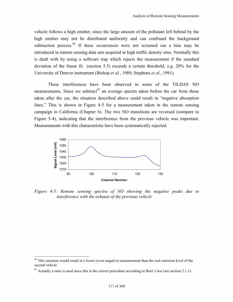
Analysis of Remote Sensing Measurements

111 of 360

vehicle follows a high emitter, since the large amount of the pollutant left behind by the

high emitter may not be distributed uniformly and can confound the background

subtraction process.96 If these occurrences were not screened out a bias may be

introduced in remote sensing data sets acquired at high traffic density sites. Normally this

is dealt with by using a software trap which rejects the measurement if the standard

deviation of the linear fit (section 5.3) exceeds a certain threshold, e.g. 20% for the

University of Denver instrument (Bishop et al., 1989; Stephens et al., 1991).

These interferences have been observed in some of the TILDAS NO

measurements. Since we subtract97 an average spectra taken before the car from those

taken after the car, the situation described above could result in “negative absorption

lines.” This is shown in Figure 4-5 for a measurement taken in the remote sensing

campaign in California (Chapter 6). The two NO transitions are reversed (compare to

Figure 5-4), indicating that the interference from the previous vehicle was important.

Measurements with this characteristic have been systematically rejected.

1010

1020

1030

1040

1050

1060

90 100 110 120 130

Channel Number

Sig

nal

Lev

el (

mV

)

Figure 4-5: Remote sensing spectra of NO showing the negative peaks due tointerference with the exhaust of the previous vehicle

96 This situation would result in a lower (even negative) measurement than the real emission level of thesecond vehicle.97 Actually a ratio is used since this is the correct procedure according to Beer’s law (see section 2.1.1).

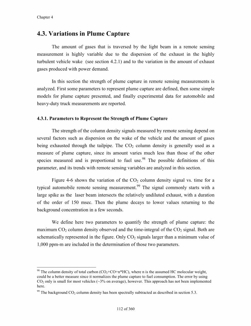
Chapter 4

112 of 360

4.3. Variations in Plume Capture

The amount of gases that is traversed by the light beam in a remote sensing

measurement is highly variable due to the dispersion of the exhaust in the highly

turbulent vehicle wake (see section 4.2.1) and to the variation in the amount of exhaust

gases produced with power demand.

In this section the strength of plume capture in remote sensing measurements is

analyzed. First some parameters to represent plume capture are defined, then some simple

models for plume capture presented, and finally experimental data for automobile and

heavy-duty truck measurements are reported.

4.3.1. Parameters to Represent the Strength of Plume Capture

The strength of the column density signals measured by remote sensing depend on

several factors such as dispersion on the wake of the vehicle and the amount of gases

being exhausted through the tailpipe. The CO2 column density is generally used as a

measure of plume capture, since its amount varies much less than those of the other

species measured and is proportional to fuel use.98 The possible definitions of this

parameter, and its trends with remote sensing variables are analyzed in this section.

Figure 4-6 shows the variation of the CO2 column density signal vs. time for a

typical automobile remote sensing measurement.99 The signal commonly starts with a

large spike as the laser beam intersects the relatively undiluted exhaust, with a duration

of the order of 150 msec. Then the plume decays to lower values returning to the

background concentration in a few seconds.

We define here two parameters to quantify the strength of plume capture: the

maximum CO2 column density observed and the time-integral of the CO2 signal. Both are

schematically represented in the figure. Only CO2 signals larger than a minimum value of

1,000 ppm-m are included in the determination of those two parameters.

98 The column density of total carbon (CO2+CO+n*HC), where n is the assumed HC molecular weight,could be a better measure since it normalizes the plume capture to fuel consumption. The error by usingCO2 only is small for most vehicles (~3% on average), however. This approach has not been implementedhere.99 The background CO2 column density has been spectrally subtracted as described in section 5.3.

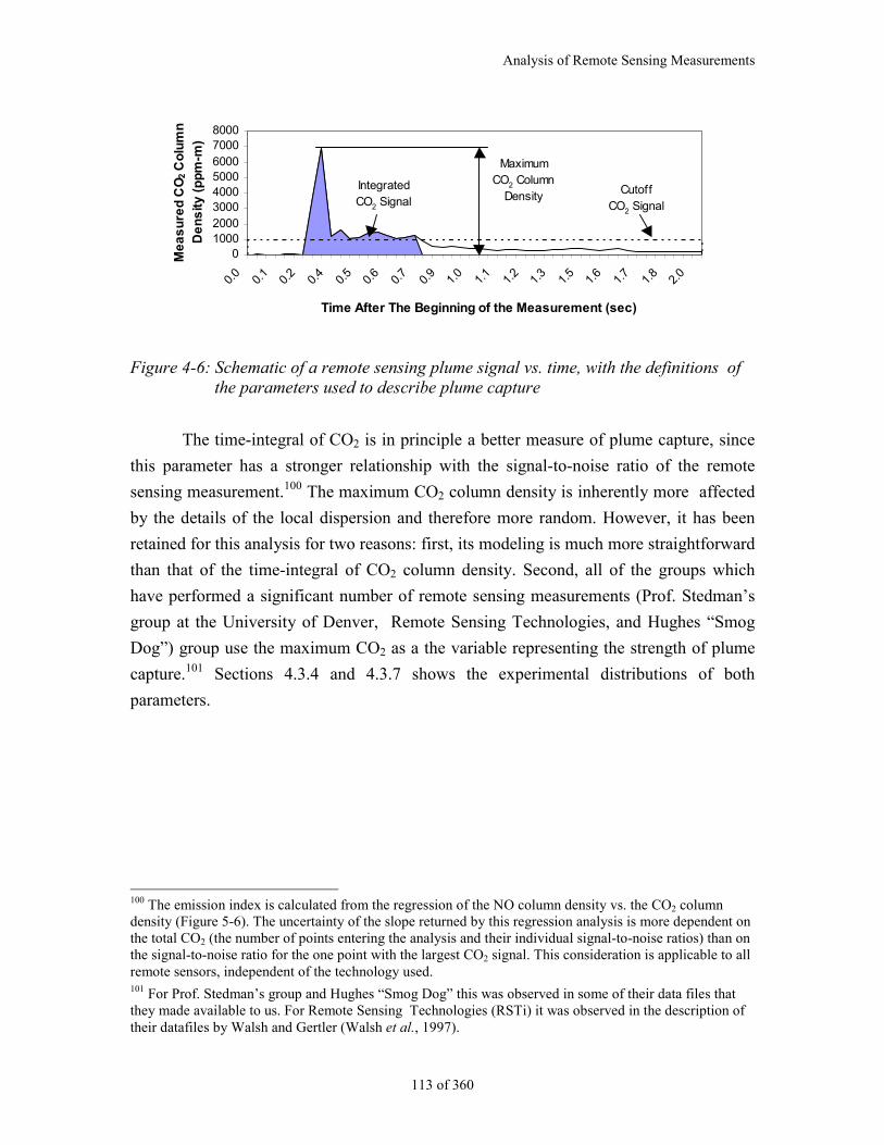
Analysis of Remote Sensing Measurements

113 of 360

010002000300040005000600070008000

0.0

0.1

0.2

0.4

0.5

0.6

0.7

0.9

1.0

1.1

1.2

1.3

1.5

1.6

1.7

1.8

2.0

Time After The Beginning of the Measurement (sec)

Me

as

ure

d C

O2

Co

lum

n

De

ns

ity

(p

pm

-m)

MaximumCO2 Column

DensityIntegratedCO2 Signal

CutoffCO2 Signal

Figure 4-6: Schematic of a remote sensing plume signal vs. time, with the definitions ofthe parameters used to describe plume capture

The time-integral of CO2 is in principle a better measure of plume capture, since

this parameter has a stronger relationship with the signal-to-noise ratio of the remote

sensing measurement.100 The maximum CO2 column density is inherently more affected

by the details of the local dispersion and therefore more random. However, it has been

retained for this analysis for two reasons: first, its modeling is much more straightforward

than that of the time-integral of CO2 column density. Second, all of the groups which

have performed a significant number of remote sensing measurements (Prof. Stedman’s

group at the University of Denver, Remote Sensing Technologies, and Hughes “Smog

Dog”) group use the maximum CO2 as a the variable representing the strength of plume

capture.101 Sections 4.3.4 and 4.3.7 shows the experimental distributions of both

parameters.

100 The emission index is calculated from the regression of the NO column density vs. the CO2 columndensity (Figure 5-6). The uncertainty of the slope returned by this regression analysis is more dependent onthe total CO2 (the number of points entering the analysis and their individual signal-to-noise ratios) than onthe signal-to-noise ratio for the one point with the largest CO2 signal. This consideration is applicable to allremote sensors, independent of the technology used.101 For Prof. Stedman’s group and Hughes “Smog Dog” this was observed in some of their data files thatthey made available to us. For Remote Sensing Technologies (RSTi) it was observed in the description oftheir datafiles by Walsh and Gertler (Walsh et al., 1997).

Chapter 4

114 of 360

4.3.2. Expected CO2 Column Density in Automobile Remote Sensing: Fluid

Mechanical Model

The flow of the gases exiting the tailpipe is an axial jet in a rather complicated

bluff-body wake, which normally features a recirculation zone attached to the vehicle

near the tailpipe (see section 4.2.1).

As a first approximation to estimate the signal levels that can be expected on

remote sensing an unperturbed axial jet can be assumed. A visualization of such a jet is

shown in Figure 4-7 (Kurima et al., 1994). A general characteristic of these jets is the

existence of a “potential core” which lasts a few nozzle diameters (Beer and Chigier,

1972) where the jet has not mixed with the surrounding fluid.

Figure 4-7: Visualization of an axisymmetric jet showing the potential core and the jetbreakup and mixing region

A remote sensing system such as the TILDAS instrument described in section 5.2

sends a light beam across the road to a retro-reflector which then returns the beam to an

optical detector. Under ideal conditions both the outgoing and the incoming light beams

would traverse the undiluted exhaust for a distance of 2 tailpipe diameters, as shown in

Figure 4-8. This is what we call the “direct hit” model.

The tailpipe diameter of a typical automobile is 2 inches or 5 cm and the exhaust

CO2 concentration is about 13.4% for stoichiometric combustion. This yields a “direct

hit” signal strength of 13,400 ppm-m. The signal strengths observed in the real world are

of this order. Signal strengths lower than 1,000 ppm-m CO2 are rejected as too low for

good signal-to-noise ratio.

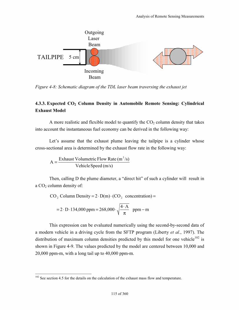
Analysis of Remote Sensing Measurements

115 of 360

��������������������������������������������������

����������������������������������

OutgoingLaser Beam

Incoming Beam

TAILPIPE 5 cm

����������������������������������������������������������������������������������������������������������������������������������������������������������������������������������������������������������������������������

�����������������������������������������������������������������������������������������������������������������������������������������������������������������������������������������������������������������������������������������������������������������������������������

Figure 4-8: Schematic diagram of the TDL laser beam traversing the exhaust jet

4.3.3. Expected CO2 Column Density in Automobile Remote Sensing: Cylindrical

Exhaust Model

A more realistic and flexible model to quantify the CO2 column density that takes

into account the instantaneous fuel economy can be derived in the following way:

Let’s assume that the exhaust plume leaving the tailpipe is a cylinder whose

cross-sectional area is determined by the exhaust flow rate in the following way:

(m/s) Speed Vehicle

/s)(m Rate Flow VolumetricExhaust A

3

=

Then, calling D the plume diameter, a “direct hit” of such a cylinder will result in

a CO2 column density of:

mppm A 4

268,000 ppm 134,000 D 2

ion)concentrat (CO D(m) 2 Density Column CO 22

−π⋅⋅=⋅⋅=

=⋅⋅=

This expression can be evaluated numerically using the second-by-second data of

a modern vehicle in a driving cycle from the SFTP program (Liberty et al., 1997). The

distribution of maximum column densities predicted by this model for one vehicle102 is

shown in Figure 4-9. The values predicted by the model are centered between 10,000 and

20,000 ppm-m, with a long tail up to 40,000 ppm-m.

102 See section 4.5 for the details on the calculation of the exhaust mass flow and temperature.

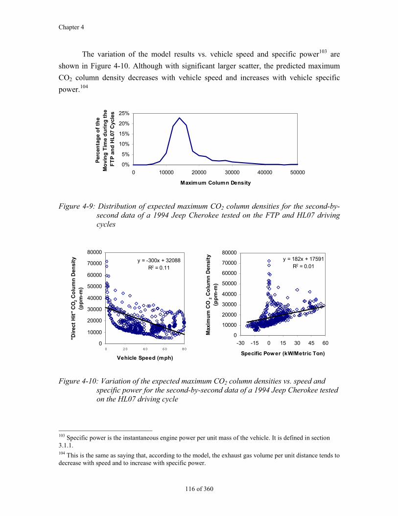
Chapter 4

116 of 360

The variation of the model results vs. vehicle speed and specific power103 are

shown in Figure 4-10. Although with significant larger scatter, the predicted maximum

CO2 column density decreases with vehicle speed and increases with vehicle specific

power.104

0%

5%

10%

15%

20%

25%

0 10000 20000 30000 40000 50000

Maximum Column Density

Per

cen

tag

e o

f th

e M

ovi

ng

Tim

e d

uri

ng

th

e F

TP

an

d H

L07

Cyc

les

Figure 4-9: Distribution of expected maximum CO2 column densities for the second-by-second data of a 1994 Jeep Cherokee tested on the FTP and HL07 drivingcycles

y = 182x + 17591R2 = 0.01

0

10000

20000

30000

40000

50000

60000

70000

80000

-30 -15 0 15 30 45 60

Specific Power (kW/Metric Ton)

Max

imu

m C

O2 C

olu

mn

Den

sity

(p

pm

-m)

y = -300x + 32088R2 = 0.11

0

10000

20000

30000

40000

50000

60000

70000

80000

0 20 40 60 80

Vehicle Speed (mph)

"Dir

ect

Hit

" C

O2 C

olu

mn

Den

sity

(p

pm

-m)

8

Figure 4-10: Variation of the expected maximum CO2 column densities vs. speed andspecific power for the second-by-second data of a 1994 Jeep Cherokee testedon the HL07 driving cycle

103 Specific power is the instantaneous engine power per unit mass of the vehicle. It is defined in section3.1.1.104 This is the same as saying that, according to the model, the exhaust gas volume per unit distance tends todecrease with speed and to increase with specific power.

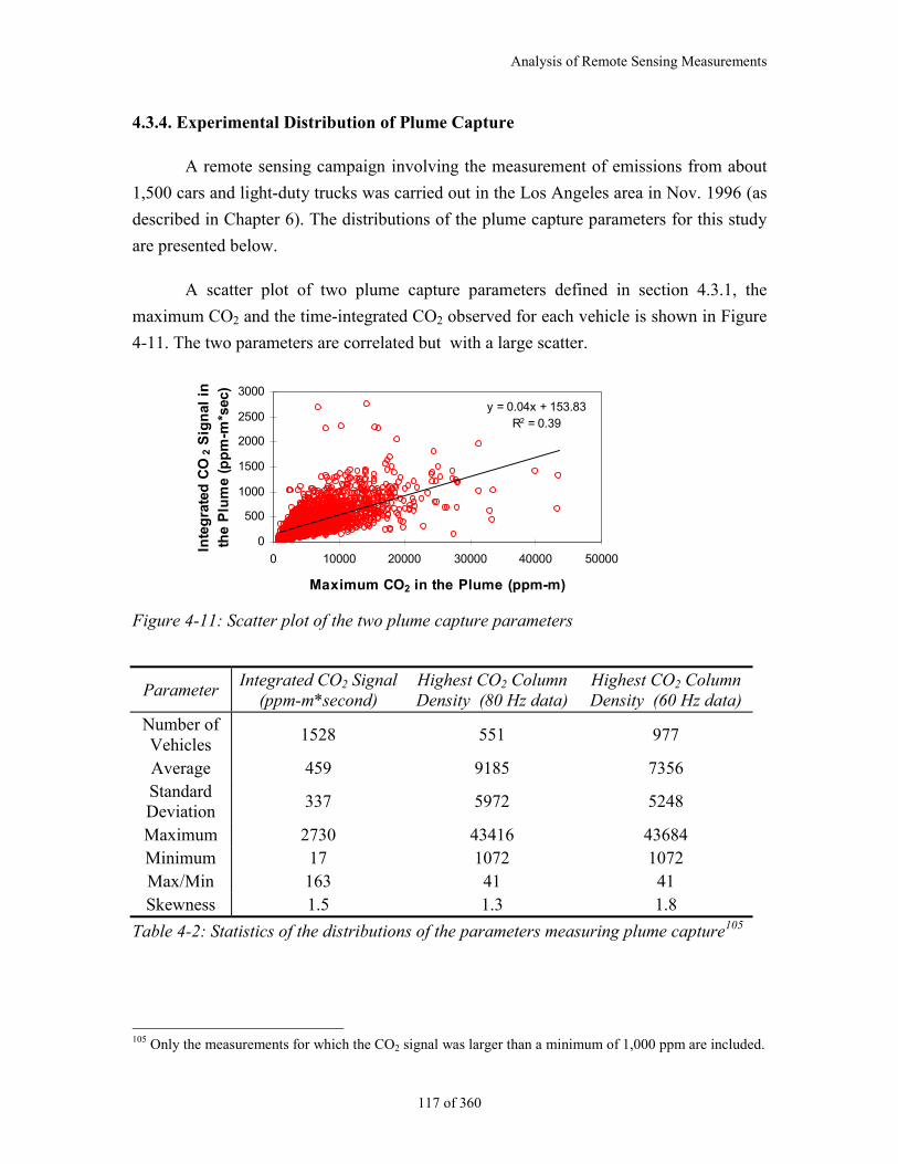
Analysis of Remote Sensing Measurements

117 of 360

4.3.4. Experimental Distribution of Plume Capture

A remote sensing campaign involving the measurement of emissions from about

1,500 cars and light-duty trucks was carried out in the Los Angeles area in Nov. 1996 (as

described in Chapter 6). The distributions of the plume capture parameters for this study

are presented below.

A scatter plot of two plume capture parameters defined in section 4.3.1, the

maximum CO2 and the time-integrated CO2 observed for each vehicle is shown in Figure

4-11. The two parameters are correlated but with a large scatter.

y = 0.04x + 153.83R2 = 0.39

0

500

1000

1500

2000

2500

3000

0 10000 20000 30000 40000 50000

Maximum CO2 in the Plume (ppm-m)

Inte

gra

ted

CO

2 S

ign

al i

n

the

Plu

me

(pp

m-m

*sec

)

Figure 4-11: Scatter plot of the two plume capture parameters

ParameterIntegrated CO2 Signal

(ppm-m*second)Highest CO2 ColumnDensity (80 Hz data)

Highest CO2 ColumnDensity (60 Hz data)

Number ofVehicles

1528 551 977

Average 459 9185 7356StandardDeviation

337 5972 5248

Maximum 2730 43416 43684Minimum 17 1072 1072Max/Min 163 41 41Skewness 1.5 1.3 1.8

Table 4-2: Statistics of the distributions of the parameters measuring plume capture105

105 Only the measurements for which the CO2 signal was larger than a minimum of 1,000 ppm are included.

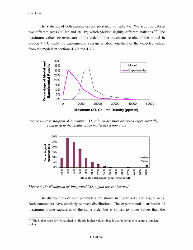
Chapter 4

118 of 360

The statistics of both parameters are presented in Table 4-2. We acquired data at

two different rates (60 Hz and 80 Hz) which yielded slightly different statistics.106 The

maximum values observed are of the order of the maximum results of the model in

section 4.3.3, while the experimental average is about one-half of the expected values

from the models in sections 4.3.2 and 4.3.3.

0%

5%

10%

15%

20%

25%

30%

35%

40%

0 10000 20000 30000 40000 50000

Maximum CO2 Column Density (ppm-m)

Pe

rce

nta

ge

of

Mo

de

l a

nd

E

xp

eri

me

nta

l R

es

ult

s Model

Experimental

Figure 4-12: Histogram of maximum CO2 column densities observed experimentally,compared to the results of the model in section 4.3.3

0%

5%

10%

15%

20%

25%

30%

< 20

0

200

400

600

800

1000

1200

1400

1600

1800

2000

2200

2400

2600

2800

Integrated CO2 Signal (ppm-m*second)

Per

cen

tag

e o

f M

easu

rem

ents

MaximumValue

Figure 4-13: Histogram of integrated CO2 signal levels observed

The distributions of both parameters are shown in Figure 4-12 and Figure 4-13.

Both parameters have similarly skewed distributions. The experimental distribution of

maximum plume capture is of the same order but is shifted to lower values than the

106 The higher rate (80 Hz) resulted in slightly higher values since it was better able to capture transientspikes.

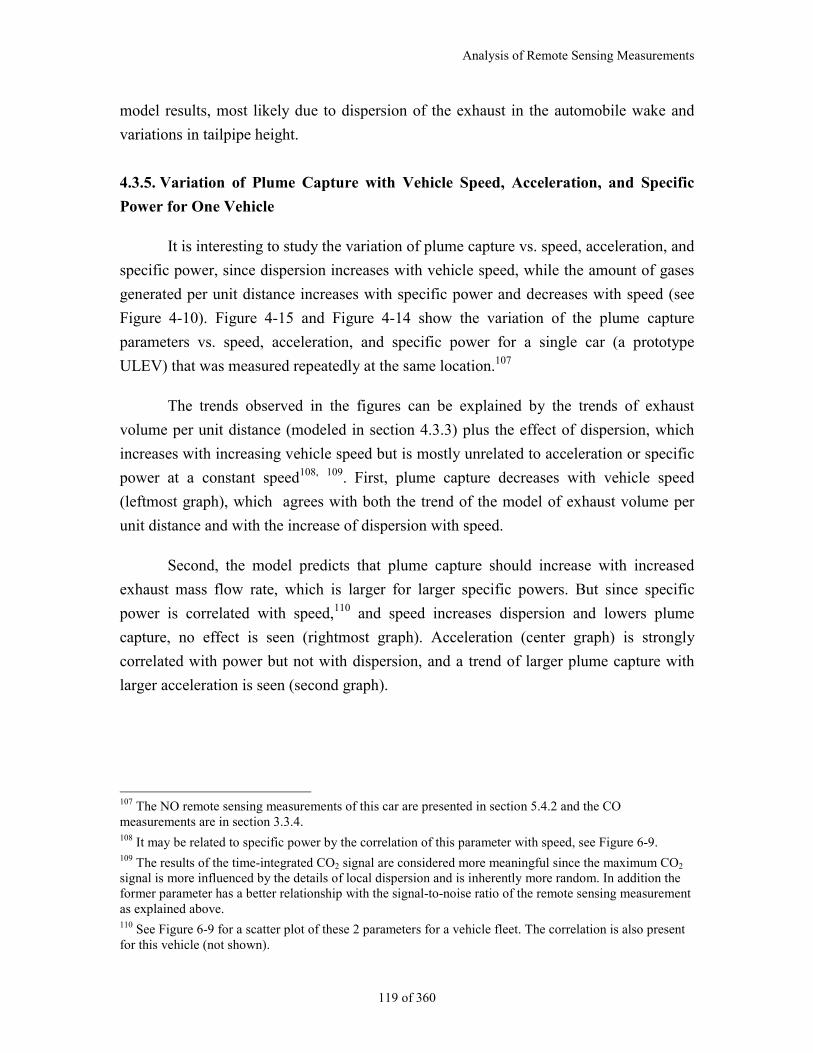
Analysis of Remote Sensing Measurements

119 of 360

model results, most likely due to dispersion of the exhaust in the automobile wake and

variations in tailpipe height.

4.3.5. Variation of Plume Capture with Vehicle Speed, Acceleration, and Specific

Power for One Vehicle

It is interesting to study the variation of plume capture vs. speed, acceleration, and

specific power, since dispersion increases with vehicle speed, while the amount of gases

generated per unit distance increases with specific power and decreases with speed (see

Figure 4-10). Figure 4-15 and Figure 4-14 show the variation of the plume capture

parameters vs. speed, acceleration, and specific power for a single car (a prototype

ULEV) that was measured repeatedly at the same location.107

The trends observed in the figures can be explained by the trends of exhaust

volume per unit distance (modeled in section 4.3.3) plus the effect of dispersion, which

increases with increasing vehicle speed but is mostly unrelated to acceleration or specific

power at a constant speed108, 109. First, plume capture decreases with vehicle speed

(leftmost graph), which agrees with both the trend of the model of exhaust volume per

unit distance and with the increase of dispersion with speed.

Second, the model predicts that plume capture should increase with increased

exhaust mass flow rate, which is larger for larger specific powers. But since specific

power is correlated with speed,110 and speed increases dispersion and lowers plume

capture, no effect is seen (rightmost graph). Acceleration (center graph) is strongly

correlated with power but not with dispersion, and a trend of larger plume capture with

larger acceleration is seen (second graph).

107 The NO remote sensing measurements of this car are presented in section 5.4.2 and the COmeasurements are in section 3.3.4.108 It may be related to specific power by the correlation of this parameter with speed, see Figure 6-9.109 The results of the time-integrated CO2 signal are considered more meaningful since the maximum CO2

signal is more influenced by the details of local dispersion and is inherently more random. In addition theformer parameter has a better relationship with the signal-to-noise ratio of the remote sensing measurementas explained above.110 See Figure 6-9 for a scatter plot of these 2 parameters for a vehicle fleet. The correlation is also presentfor this vehicle (not shown).

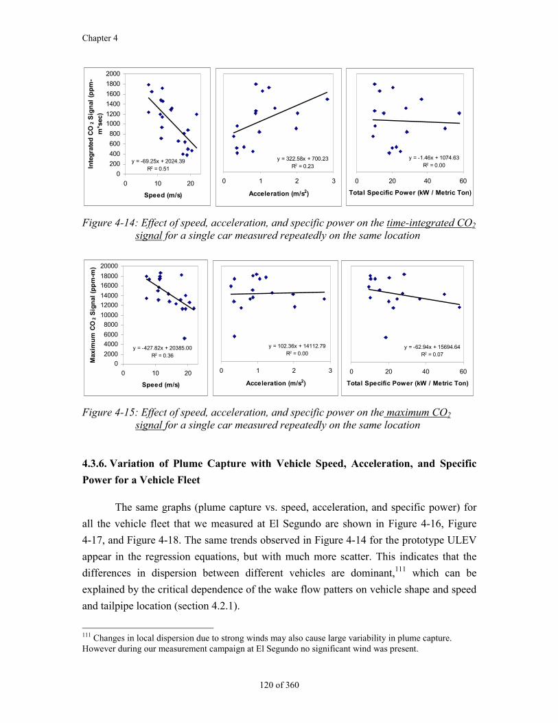
Chapter 4

120 of 360

y = -1.46x + 1074.63R2 = 0.00

0 20 40 60

Total Specific Power (kW / Metric Ton)

y = 322.58x + 700.23R2 = 0.23

0 1 2 3

Acceleration (m/s2)

y = -69.25x + 2024.39R2 = 0.51

0

200

400

600

800

1000

1200

1400

1600

1800

2000

0 10 20

Speed (m/s)

Inte

gra

ted

CO

2 S

ign

al (

pp

m-

m*s

ec)

Figure 4-14: Effect of speed, acceleration, and specific power on the time-integrated CO2

signal for a single car measured repeatedly on the same location

y = -427.82x + 20385.00R2 = 0.36

0

2000

4000

6000

8000

10000

12000

14000

16000

18000

20000

0 10 20

Speed (m/s)

Max

imu

m C

O2 S

ign

al (

pp

m-m

)

y = 102.36x + 14112.79R2 = 0.00

0 1 2 3

Acceleration (m/s2)

y = -62.94x + 15694.64R2 = 0.07

0 20 40 60

Total Specific Power (kW / Metric Ton)

Figure 4-15: Effect of speed, acceleration, and specific power on the maximum CO2

signal for a single car measured repeatedly on the same location

4.3.6. Variation of Plume Capture with Vehicle Speed, Acceleration, and Specific

Power for a Vehicle Fleet

The same graphs (plume capture vs. speed, acceleration, and specific power) for

all the vehicle fleet that we measured at El Segundo are shown in Figure 4-16, Figure

4-17, and Figure 4-18. The same trends observed in Figure 4-14 for the prototype ULEV

appear in the regression equations, but with much more scatter. This indicates that the

differences in dispersion between different vehicles are dominant,111 which can be

explained by the critical dependence of the wake flow patters on vehicle shape and speed

and tailpipe location (section 4.2.1).

111 Changes in local dispersion due to strong winds may also cause large variability in plume capture.However during our measurement campaign at El Segundo no significant wind was present.

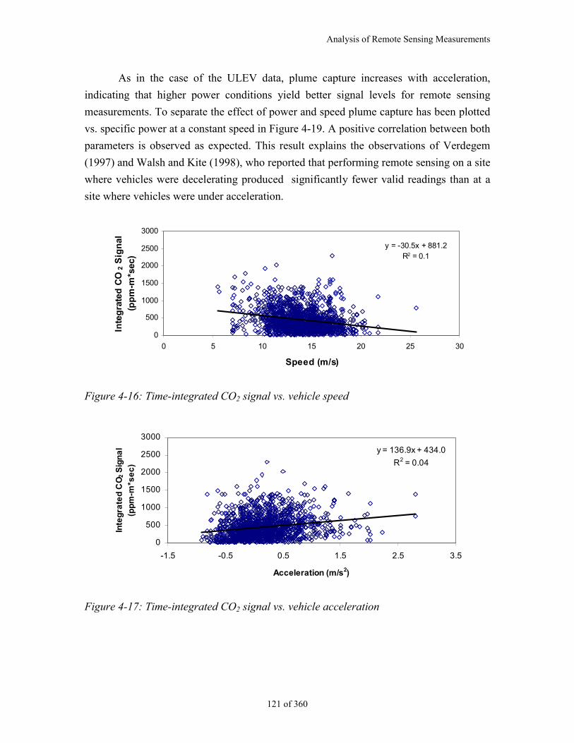
Analysis of Remote Sensing Measurements

121 of 360

As in the case of the ULEV data, plume capture increases with acceleration,

indicating that higher power conditions yield better signal levels for remote sensing

measurements. To separate the effect of power and speed plume capture has been plotted

vs. specific power at a constant speed in Figure 4-19. A positive correlation between both

parameters is observed as expected. This result explains the observations of Verdegem

(1997) and Walsh and Kite (1998), who reported that performing remote sensing on a site

where vehicles were decelerating produced significantly fewer valid readings than at a

site where vehicles were under acceleration.

y = -30.5x + 881.2R2 = 0.1

0

500

1000

1500

2000

2500

3000

0 5 10 15 20 25 30

Speed (m/s)

Inte

gra

ted

CO

2 S

ign

al

(pp

m-m

*sec

)

Figure 4-16: Time-integrated CO2 signal vs. vehicle speed

y = 136.9x + 434.0

R2 = 0.04

0

500

1000

1500

2000

2500

3000

-1.5 -0.5 0.5 1.5 2.5 3.5

Acceleration (m/s2)

Inte

gra

ted

CO

2 S

ign

al

(pp

m-m

*se

c)

Figure 4-17: Time-integrated CO2 signal vs. vehicle acceleration

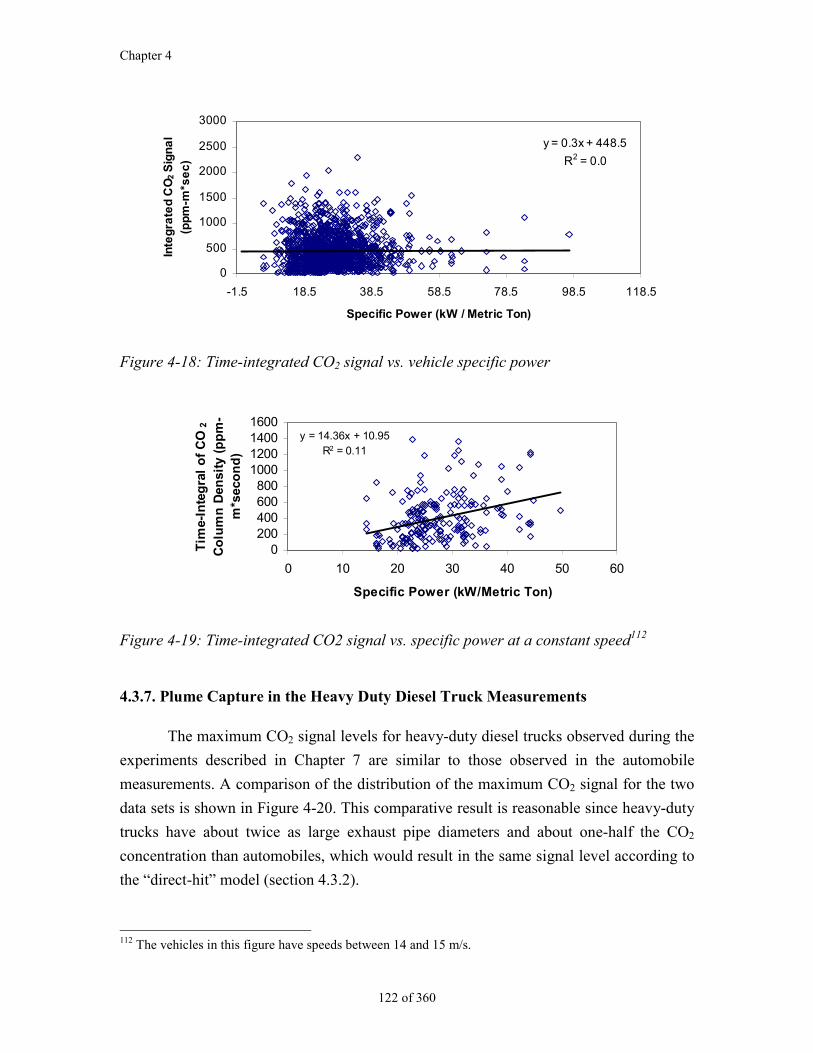
Chapter 4

122 of 360

y = 0.3x + 448.5

R2 = 0.0

0

500

1000

1500

2000

2500

3000

-1.5 18.5 38.5 58.5 78.5 98.5 118.5

Specific Power (kW / Metric Ton)

Inte

gra

ted

CO

2 S

ign

al

(pp

m-m

*se

c)

Figure 4-18: Time-integrated CO2 signal vs. vehicle specific power

y = 14.36x + 10.95R2 = 0.11

0200400600800

1000120014001600

0 10 20 30 40 50 60

Specific Power (kW/Metric Ton)

Tim

e-In

teg

ral

of

CO

2

Co

lum

n D

ensi

ty (

pp

m-

m*s

eco

nd

)

Figure 4-19: Time-integrated CO2 signal vs. specific power at a constant speed112

4.3.7. Plume Capture in the Heavy Duty Diesel Truck Measurements

The maximum CO2 signal levels for heavy-duty diesel trucks observed during the

experiments described in Chapter 7 are similar to those observed in the automobile

measurements. A comparison of the distribution of the maximum CO2 signal for the two

data sets is shown in Figure 4-20. This comparative result is reasonable since heavy-duty

trucks have about twice as large exhaust pipe diameters and about one-half the CO2

concentration than automobiles, which would result in the same signal level according to

the “direct-hit” model (section 4.3.2).

112 The vehicles in this figure have speeds between 14 and 15 m/s.

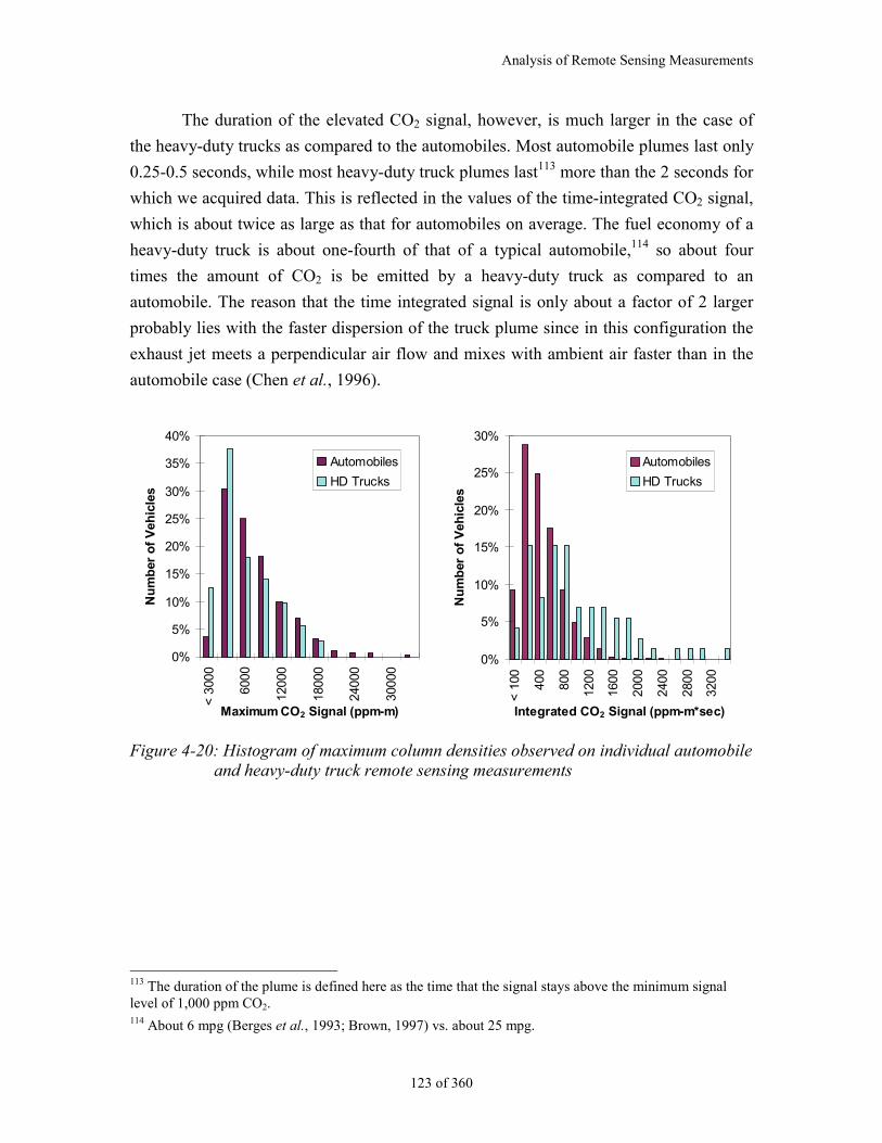
Analysis of Remote Sensing Measurements

123 of 360

The duration of the elevated CO2 signal, however, is much larger in the case of

the heavy-duty trucks as compared to the automobiles. Most automobile plumes last only

0.25-0.5 seconds, while most heavy-duty truck plumes last113 more than the 2 seconds for

which we acquired data. This is reflected in the values of the time-integrated CO2 signal,

which is about twice as large as that for automobiles on average. The fuel economy of a

heavy-duty truck is about one-fourth of that of a typical automobile,114 so about four

times the amount of CO2 is be emitted by a heavy-duty truck as compared to an

automobile. The reason that the time integrated signal is only about a factor of 2 larger

probably lies with the faster dispersion of the truck plume since in this configuration the

exhaust jet meets a perpendicular air flow and mixes with ambient air faster than in the

automobile case (Chen et al., 1996).

0%

5%

10%

15%

20%

25%

30%

35%

40%

< 3

000

6000

1200

0

1800

0

2400

0

3000

0

Maximum CO2 Signal (ppm-m)

Nu

mb

er o

f V

ehic

les

Automobiles

HD Trucks

0%

5%

10%

15%

20%

25%

30%

< 1

00 400

800

1200

1600

2000

2400

2800

3200

Integrated CO2 Signal (ppm-m*sec)

Nu

mb

er o

f V

ehic

les

Automobiles

HD Trucks

Figure 4-20: Histogram of maximum column densities observed on individual automobileand heavy-duty truck remote sensing measurements

113 The duration of the plume is defined here as the time that the signal stays above the minimum signallevel of 1,000 ppm CO2.114 About 6 mpg (Berges et al., 1993; Brown, 1997) vs. about 25 mpg.

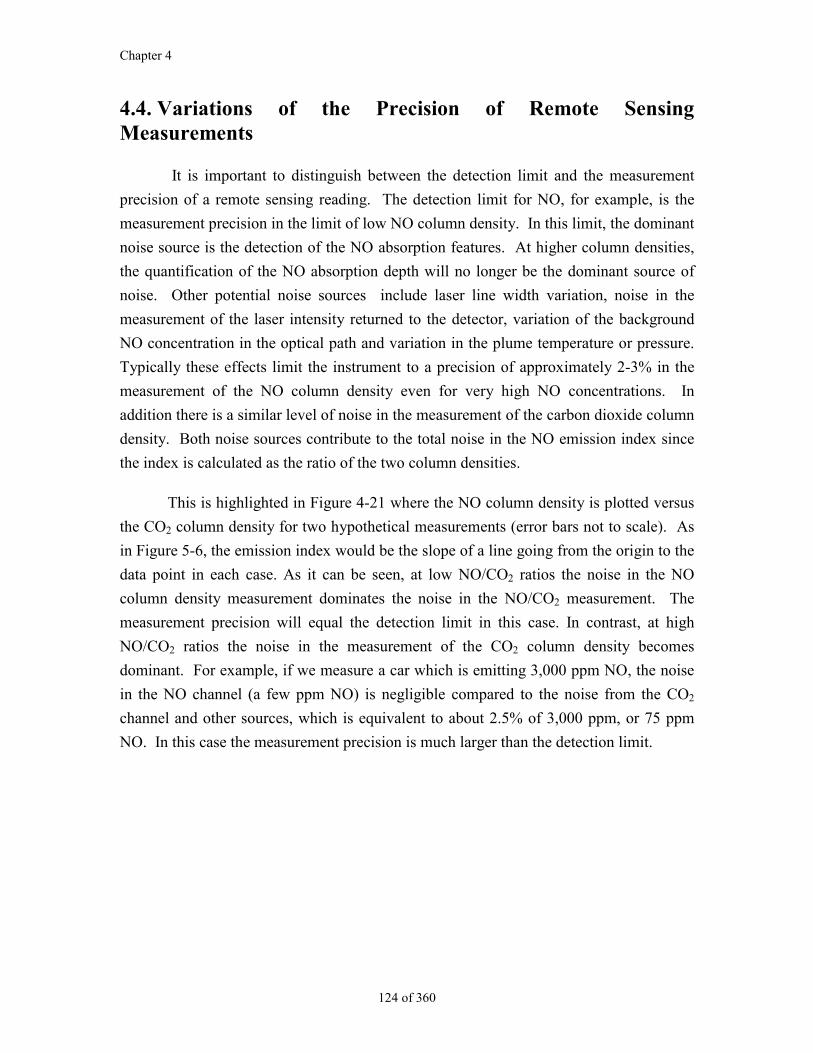
Chapter 4

124 of 360

4.4. Variations of the Precision of Remote SensingMeasurements

It is important to distinguish between the detection limit and the measurement

precision of a remote sensing reading. The detection limit for NO, for example, is the

measurement precision in the limit of low NO column density. In this limit, the dominant

noise source is the detection of the NO absorption features. At higher column densities,

the quantification of the NO absorption depth will no longer be the dominant source of

noise. Other potential noise sources include laser line width variation, noise in the

measurement of the laser intensity returned to the detector, variation of the background

NO concentration in the optical path and variation in the plume temperature or pressure.

Typically these effects limit the instrument to a precision of approximately 2-3% in the

measurement of the NO column density even for very high NO concentrations. In

addition there is a similar level of noise in the measurement of the carbon dioxide column

density. Both noise sources contribute to the total noise in the NO emission index since

the index is calculated as the ratio of the two column densities.

This is highlighted in Figure 4-21 where the NO column density is plotted versus

the CO2 column density for two hypothetical measurements (error bars not to scale). As

in Figure 5-6, the emission index would be the slope of a line going from the origin to the

data point in each case. As it can be seen, at low NO/CO2 ratios the noise in the NO

column density measurement dominates the noise in the NO/CO2 measurement. The

measurement precision will equal the detection limit in this case. In contrast, at high

NO/CO2 ratios the noise in the measurement of the CO2 column density becomes

dominant. For example, if we measure a car which is emitting 3,000 ppm NO, the noise

in the NO channel (a few ppm NO) is negligible compared to the noise from the CO2

channel and other sources, which is equivalent to about 2.5% of 3,000 ppm, or 75 ppm

NO. In this case the measurement precision is much larger than the detection limit.

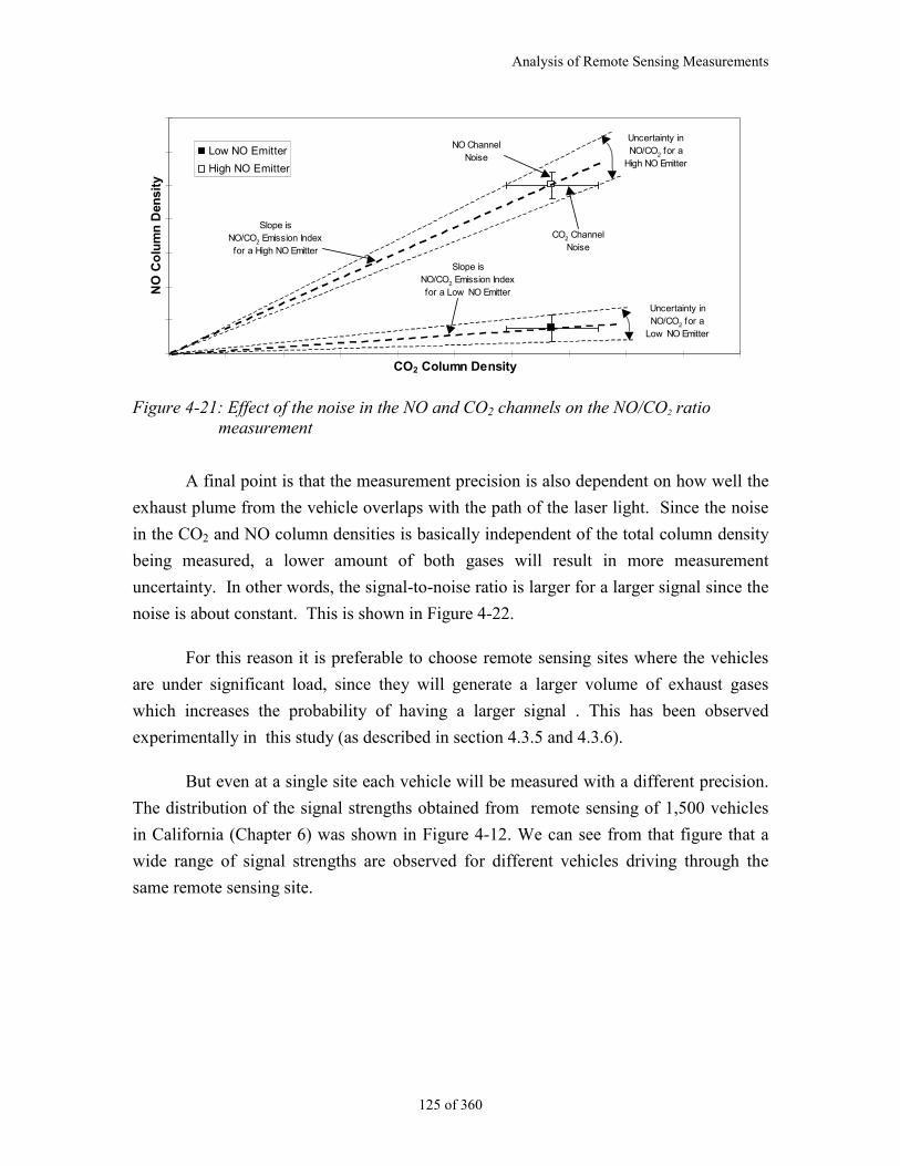
Analysis of Remote Sensing Measurements

125 of 360

CO2 Column Density

NO

Co

lum

n D

ensi

tyLow NO Emitter

High NO Emitter

Uncertainty in NO/CO2 for a

High NO Emitter

Uncertainty in NO/CO2 for a

Low NO Emitter

Slope isNO/CO2 Emission Indexfor a High NO Emitter

Slope isNO/CO2 Emission Indexfor a Low NO Emitter

CO2 Channel Noise

NO Channel Noise

Figure 4-21: Effect of the noise in the NO and CO2 channels on the NO/CO2 ratiomeasurement

A final point is that the measurement precision is also dependent on how well the

exhaust plume from the vehicle overlaps with the path of the laser light. Since the noise

in the CO2 and NO column densities is basically independent of the total column density

being measured, a lower amount of both gases will result in more measurement

uncertainty. In other words, the signal-to-noise ratio is larger for a larger signal since the

noise is about constant. This is shown in Figure 4-22.

For this reason it is preferable to choose remote sensing sites where the vehicles

are under significant load, since they will generate a larger volume of exhaust gases

which increases the probability of having a larger signal . This has been observed

experimentally in this study (as described in section 4.3.5 and 4.3.6).

But even at a single site each vehicle will be measured with a different precision.

The distribution of the signal strengths obtained from remote sensing of 1,500 vehicles

in California (Chapter 6) was shown in Figure 4-12. We can see from that figure that a

wide range of signal strengths are observed for different vehicles driving through the

same remote sensing site.

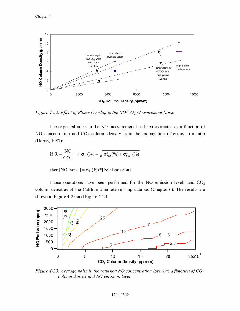
Chapter 4

126 of 360

0

2

4

6

8

10

12

0 3000 6000 9000 12000 15000

CO2 Column Density (ppm-m)

NO

Co

lum

n D

en

sity

(p

pm

-m)

Uncertainty in NO/CO2 w ithhigh plume

overlap

High plume overlap case

Low plume overlap caseUncertainty in

NO/CO2 w ithlow plumeoverlap

Figure 4-22: Effect of Plume Overlap in the NO/CO2 Measurement Noise

The expected noise in the NO measurement has been estimated as a function of

NO concentration and CO2 column density from the propagation of errors in a ratio

(Harris, 1987):

(%) (%) (%) CO

NOR if 2

CO2NOR

22

σ+σ=σ⇒=

]Emission NO[*(%)noise] [NOthen Rσ=

Those operations have been performed for the NO emission levels and CO2

column densities of the California remote sensing data set (Chapter 6). The results are

shown in Figure 4-23 and Figure 4-24.

3000

2500

2000

1500

1000

500

0

NO

Em

iss

ion

(p

pm

)

25x103 20151050

CO2 Column Density (ppm-m)

50

25

10

5

5

5

2.5

10

20

0

50

75

Figure 4-23: Average noise in the returned NO concentration (ppm) as a function of CO2

column density and NO emission level

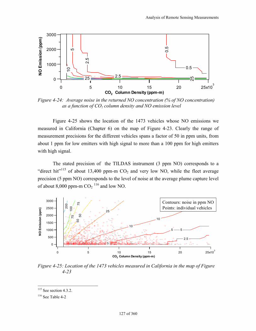
Analysis of Remote Sensing Measurements

127 of 360

3000

2000

1000

0

NO

Em

iss

ion

(p

pm

)

25x103 20151050

CO2 Column Density (ppm-m)

10

5

2.5

0.5

0.5

25

25 2.5

Figure 4-24: Average noise in the returned NO concentration (% of NO concentration)as a function of CO2 column density and NO emission level

Figure 4-25 shows the location of the 1473 vehicles whose NO emissions we

measured in California (Chapter 6) on the map of Figure 4-23. Clearly the range of

measurement precisions for the different vehicles spans a factor of 50 in ppm units, from

about 1 ppm for low emitters with high signal to more than a 100 ppm for high emitters

with high signal.

The stated precision of the TILDAS instrument (3 ppm NO) corresponds to a

“direct hit”115 of about 13,400 ppm-m CO2 and very low NO, while the fleet average

precision (5 ppm NO) corresponds to the level of noise at the average plume capture level

of about 8,000 ppm-m CO2 116 and low NO.

3000

2500

2000

1500

1000

500

0

NO

Em

iss

ion

(p

pm

)

25x103 20151050

CO2 Column Density (ppm-m)

10

0 7

5

50

25

10

5

5

5

2.5

10

20

0

50

75

Contours: noise in ppm NOPoints: individual vehicles

Figure 4-25: Location of the 1473 vehicles measured in California in the map of Figure4-23

115 See section 4.3.2.116 See Table 4-2

Chapter 4

128 of 360

The points illustrated in this section are applicable to all remote sensing

instruments independent of the particular spectroscopic technology being used.

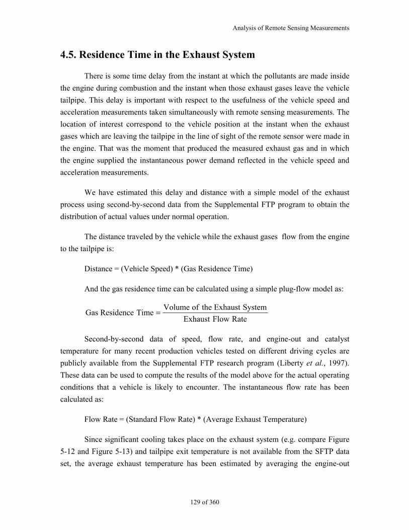
Analysis of Remote Sensing Measurements

129 of 360

4.5. Residence Time in the Exhaust System

There is some time delay from the instant at which the pollutants are made inside

the engine during combustion and the instant when those exhaust gases leave the vehicle

tailpipe. This delay is important with respect to the usefulness of the vehicle speed and

acceleration measurements taken simultaneously with remote sensing measurements. The

location of interest correspond to the vehicle position at the instant when the exhaust

gases which are leaving the tailpipe in the line of sight of the remote sensor were made in

the engine. That was the moment that produced the measured exhaust gas and in which

the engine supplied the instantaneous power demand reflected in the vehicle speed and

acceleration measurements.

We have estimated this delay and distance with a simple model of the exhaust

process using second-by-second data from the Supplemental FTP program to obtain the

distribution of actual values under normal operation.

The distance traveled by the vehicle while the exhaust gases flow from the engine

to the tailpipe is:

Distance = (Vehicle Speed) * (Gas Residence Time)

And the gas residence time can be calculated using a simple plug-flow model as:

Rate FlowExhaust

SystemExhaust theof Volume Time Residence Gas =

Second-by-second data of speed, flow rate, and engine-out and catalyst

temperature for many recent production vehicles tested on different driving cycles are

publicly available from the Supplemental FTP research program (Liberty et al., 1997).

These data can be used to compute the results of the model above for the actual operating

conditions that a vehicle is likely to encounter. The instantaneous flow rate has been

calculated as:

Flow Rate = (Standard Flow Rate) * (Average Exhaust Temperature)

Since significant cooling takes place on the exhaust system (e.g. compare Figure

5-12 and Figure 5-13) and tailpipe exit temperature is not available from the SFTP data

set, the average exhaust temperature has been estimated by averaging the engine-out

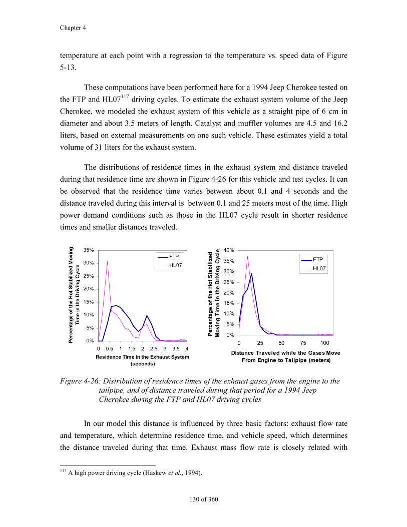
Chapter 4

130 of 360

temperature at each point with a regression to the temperature vs. speed data of Figure

5-13.

These computations have been performed here for a 1994 Jeep Cherokee tested on

the FTP and HL07117 driving cycles. To estimate the exhaust system volume of the Jeep

Cherokee, we modeled the exhaust system of this vehicle as a straight pipe of 6 cm in

diameter and about 3.5 meters of length. Catalyst and muffler volumes are 4.5 and 16.2

liters, based on external measurements on one such vehicle. These estimates yield a total

volume of 31 liters for the exhaust system.

The distributions of residence times in the exhaust system and distance traveled

during that residence time are shown in Figure 4-26 for this vehicle and test cycles. It can

be observed that the residence time varies between about 0.1 and 4 seconds and the

distance traveled during this interval is between 0.1 and 25 meters most of the time. High

power demand conditions such as those in the HL07 cycle result in shorter residence

times and smaller distances traveled.

0%

5%

10%

15%

20%

25%

30%

35%

0 0.5 1 1.5 2 2.5 3 3.5 4

Residence Time in the Exhaust System (seconds)

Pe

rce

nta

ge

of

the

Ho

t S

tab

ilize

d M

ov

ing

Tim

e in

th

e D

riv

ing

Cy

cle

FTP

HL07

0%

5%

10%

15%

20%

25%

30%

35%

40%

0 25 50 75 100

Distance Traveled while the Gases Move From Engine to Tailpipe (meters)

Per

cen

tag

e o

f th

e H

ot

Sta

bil

ized

M

ovi

ng

Tim

e in

th

e D

rivi

ng

Cyc

le

FTP

HL07

Figure 4-26: Distribution of residence times of the exhaust gases from the engine to thetailpipe, and of distance traveled during that period for a 1994 JeepCherokee during the FTP and HL07 driving cycles

In our model this distance is influenced by three basic factors: exhaust flow rate

and temperature, which determine residence time, and vehicle speed, which determines

the distance traveled during that time. Exhaust mass flow rate is closely related with

117 A high power driving cycle (Haskew et al., 1994).

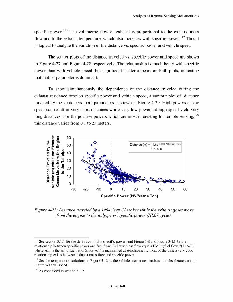
Analysis of Remote Sensing Measurements

131 of 360

specific power.118 The volumetric flow of exhaust is proportional to the exhaust mass

flow and to the exhaust temperature, which also increases with specific power.119 Thus it

is logical to analyze the variation of the distance vs. specific power and vehicle speed.

The scatter plots of the distance traveled vs. specific power and speed are shown

in Figure 4-27 and Figure 4-28 respectively. The relationship is much better with specific

power than with vehicle speed, but significant scatter appears on both plots, indicating

that neither parameter is dominant.

To show simultaneously the dependence of the distance traveled during the

exhaust residence time on specific power and vehicle speed, a contour plot of distance

traveled by the vehicle vs. both parameters is shown in Figure 4-29. High powers at low

speed can result in very short distances while very low powers at high speed yield very

long distances. For the positive powers which are most interesting for remote sensing,120

this distance varies from 0.1 to 25 meters.

Distance (m) = 14.6e-0.0346 * Specific Power

R2 = 0.30

0

10

20

30

40

50

60

-30 -20 -10 0 10 20 30 40 50 60

Specific Power (kW/Metric Ton)

Dis

tan

ce T

rave

led

by

the

Veh

icle

(m

) w

hil

e th

e E

xhau

st

Gas

es M

ove

fro

m t

he

En

gin

e to

th

e T

ailp

ipe

Figure 4-27: Distance traveled by a 1994 Jeep Cherokee while the exhaust gases movefrom the engine to the tailpipe vs. specific power (HL07 cycle)

118 See section 3.1.1 for the definition of this specific power, and Figure 3-8 and Figure 3-15 for therelationship between specific power and fuel flow. Exhaust mass flow equals EMF=(fuel flow)*(1+A/F)where A/F is the air to fuel ratio. Since A/F is maintained at stoichiometric most of the time a very goodrelationship exists between exhaust mass flow and specific power.119 See the temperature variations in Figure 5-12 as the vehicle accelerates, cruises, and decelerates, and inFigure 5-13 vs. speed.120 As concluded in section 3.2.2.

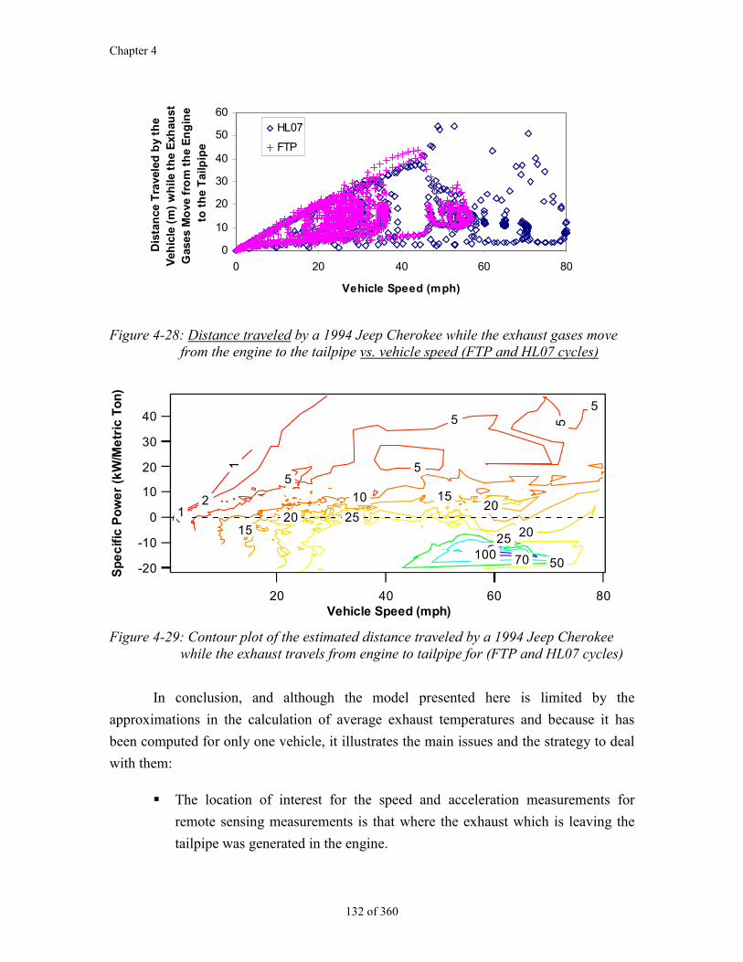
Chapter 4

132 of 360

0

10

20

30

40

50

60

0 20 40 60 80

Vehicle Speed (mph)

Dis

tan

ce T

rave

led

by

the

Veh

icle

(m

) w

hile

th

e E

xhau

st

Gas

es M

ove

fro

m t

he

En

gin

e to

th

e T

ailp

ipe

HL07

FTP

Figure 4-28: Distance traveled by a 1994 Jeep Cherokee while the exhaust gases movefrom the engine to the tailpipe vs. vehicle speed (FTP and HL07 cycles)

40

30

20

10

0

-10

-20

Sp

ec

ific

Po

we

r (k

W/M

etr

ic T

on

)

80604020 Vehicle Speed (mph)

100 70 50

25

25 20

20 20

15

15 10

5

5

5 5

5

2 1

1

Figure 4-29: Contour plot of the estimated distance traveled by a 1994 Jeep Cherokeewhile the exhaust travels from engine to tailpipe for (FTP and HL07 cycles)

In conclusion, and although the model presented here is limited by the

approximations in the calculation of average exhaust temperatures and because it has

been computed for only one vehicle, it illustrates the main issues and the strategy to deal

with them:

The location of interest for the speed and acceleration measurements for

remote sensing measurements is that where the exhaust which is leaving the

tailpipe was generated in the engine.

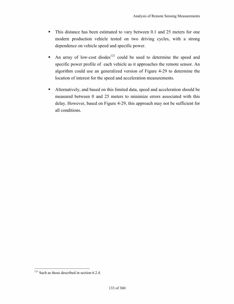
Analysis of Remote Sensing Measurements

133 of 360

This distance has been estimated to vary between 0.1 and 25 meters for one

modern production vehicle tested on two driving cycles, with a strong

dependence on vehicle speed and specific power.

An array of low-cost diodes121 could be used to determine the speed and

specific power profile of each vehicle as it approaches the remote sensor. An

algorithm could use an generalized version of Figure 4-29 to determine the

location of interest for the speed and acceleration measurements.

Alternatively, and based on this limited data, speed and acceleration should be

measured between 0 and 25 meters to minimize errors associated with this

delay. However, based on Figure 4-29, this approach may not be sufficient for

all conditions.

121 Such as those described in section 6.2.4.

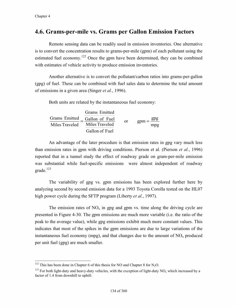
Chapter 4

134 of 360

4.6. Grams-per-mile vs. Grams per Gallon Emission Factors

Remote sensing data can be readily used in emission inventories. One alternative

is to convert the concentration results to grams-per-mile (gpm) of each pollutant using the

estimated fuel economy.122 Once the gpm have been determined, they can be combined

with estimates of vehicle activity to produce emission inventories.

Another alternative is to convert the pollutant/carbon ratios into grams-per-gallon

(gpg) of fuel. These can be combined with fuel sales data to determine the total amount

of emissions in a given area (Singer et al., 1996).

Both units are related by the instantaneous fuel economy:

mpg

gpggpmor

Fuel ofGallon

Traveled MilesFuel of Gallon

Emitted Grams

Traveled Miles

Emitted Grams ==

An advantage of the later procedure is that emission rates in gpg vary much less

than emission rates in gpm with driving conditions. Pierson et al. (Pierson et al., 1996)

reported that in a tunnel study the effect of roadway grade on gram-per-mile emission

was substantial while fuel-specific emissions were almost independent of roadway

grade.123

The variability of gpg vs. gpm emissions has been explored further here by

analyzing second by second emission data for a 1993 Toyota Corolla tested on the HL07

high power cycle during the SFTP program (Liberty et al., 1997).

The emission rates of NOx in gpg and gpm vs. time along the driving cycle are

presented in Figure 4-30. The gpm emissions are much more variable (i.e. the ratio of the

peak to the average value), while gpg emissions exhibit much more constant values. This

indicates that most of the spikes in the gpm emissions are due to large variations of the

instantaneous fuel economy (mpg), and that changes due to the amount of NOx produced

per unit fuel (gpg) are much smaller.

122 This has been done in Chapter 6 of this thesis for NO and Chapter 8 for N2O.123 For both light-duty and heavy-duty vehicles, with the exception of light-duty NOx which increased by afactor of 1.4 from downhill to uphill.

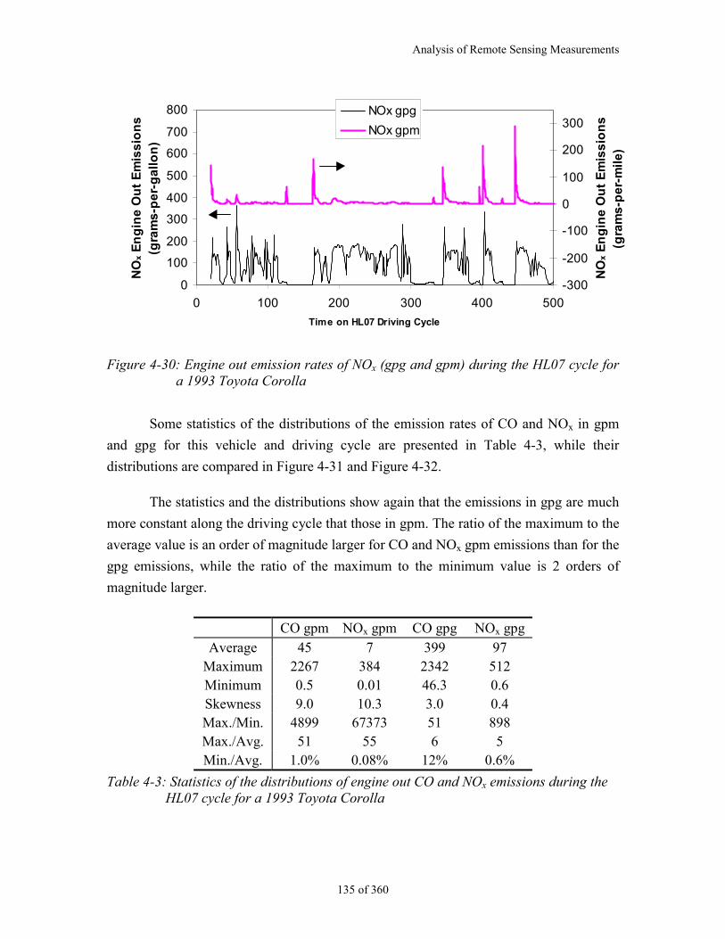
Analysis of Remote Sensing Measurements

135 of 360

0

100

200

300

400

500

600

700

800

0 100 200 300 400 500

Time on HL07 Driving Cycle

NO

x E

ng

ine

Ou

t E

mis

sio

ns

(g

ram

s-p

er-

ga

llo

n)

-300

-200

-100

0

100

200

300

NO

x E

ng

ine

Ou

t E

mis

sio

ns

(g

ram

s-p

er-

mil

e)

NOx gpg

NOx gpm

Figure 4-30: Engine out emission rates of NOx (gpg and gpm) during the HL07 cycle fora 1993 Toyota Corolla

Some statistics of the distributions of the emission rates of CO and NOx in gpm

and gpg for this vehicle and driving cycle are presented in Table 4-3, while their

distributions are compared in Figure 4-31 and Figure 4-32.

The statistics and the distributions show again that the emissions in gpg are much

more constant along the driving cycle that those in gpm. The ratio of the maximum to the

average value is an order of magnitude larger for CO and NOx gpm emissions than for the

gpg emissions, while the ratio of the maximum to the minimum value is 2 orders of

magnitude larger.

CO gpm NOx gpm CO gpg NOx gpg

Average 45 7 399 97Maximum 2267 384 2342 512Minimum 0.5 0.01 46.3 0.6Skewness 9.0 10.3 3.0 0.4Max./Min. 4899 67373 51 898Max./Avg. 51 55 6 5Min./Avg. 1.0% 0.08% 12% 0.6%

Table 4-3: Statistics of the distributions of engine out CO and NOx emissions during theHL07 cycle for a 1993 Toyota Corolla

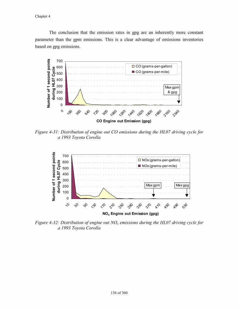
Chapter 4

136 of 360

The conclusion that the emission rates in gpg are an inherently more constant

parameter than the gpm emissions. This is a clear advantage of emissions inventories

based on gpg emissions.

0

100

200

300

400

500

600

700

018

036

054

072

090

010

8012

6014

4016

2018

0019

8021

6023

40

CO Engine out Emission (gpg)

Nu

mb

er o

f 1

seco

nd

po

ints

d

uri

ng

HL

07 C

ycle

CO (grams-per-gallon)

CO (grams-per-mile)

Max gpm & gpg

Figure 4-31: Distribution of engine out CO emissions during the HL07 driving cycle fora 1993 Toyota Corolla

0

100

200

300

400

500

600

700

10 50 90 130

170

210

250

290

330

370

410

450

490

530

NOx Engine out Emission (gpg)

Nu

mb

er o

f 1

seco

nd

po

ints

d

uri

ng

HL

07 C

ycle NOx (grams-per-gallon)

NOx (grams-per-mile)

Max gpm Max gpg

Figure 4-32: Distribution of engine out NOx emissions during the HL07 driving cycle fora 1993 Toyota Corolla

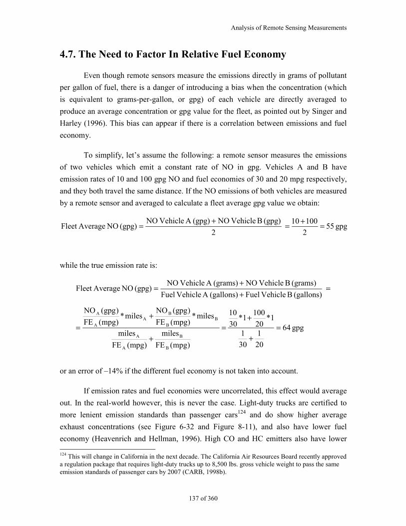
Analysis of Remote Sensing Measurements

137 of 360

4.7. The Need to Factor In Relative Fuel Economy

Even though remote sensors measure the emissions directly in grams of pollutant

per gallon of fuel, there is a danger of introducing a bias when the concentration (which

is equivalent to grams-per-gallon, or gpg) of each vehicle are directly averaged to

produce an average concentration or gpg value for the fleet, as pointed out by Singer and

Harley (1996). This bias can appear if there is a correlation between emissions and fuel

economy.

To simplify, let’s assume the following: a remote sensor measures the emissions

of two vehicles which emit a constant rate of NO in gpg. Vehicles A and B have

emission rates of 10 and 100 gpg NO and fuel economies of 30 and 20 mpg respectively,

and they both travel the same distance. If the NO emissions of both vehicles are measured

by a remote sensor and averaged to calculate a fleet average gpg value we obtain:

gpg 552

10010

2

(gpg) B Vehicle NO (gpg)A Vehicle NO(gpg) NO AverageFleet =+=

+=

while the true emission rate is:

gpg 64

20

1

30

1

1*20

1001*

30

10

)mpg(FE

miles

)mpg(FE

miles

miles*)mpg(FE

)gpg(NOmiles*

)mpg(FE

)gpg(NO

(gallons) B Vehicle Fuel (gallons)A Vehicle Fuel

(grams) B Vehicle NO (grams)A Vehicle NO(gpg) NO AverageFleet

B

B

A

A

BB

BA

A

A

=+

+=

+

+=

=++

=

or an error of –14% if the different fuel economy is not taken into account.

If emission rates and fuel economies were uncorrelated, this effect would average

out. In the real-world however, this is never the case. Light-duty trucks are certified to

more lenient emission standards than passenger cars124 and do show higher average

exhaust concentrations (see Figure 6-32 and Figure 8-11), and also have lower fuel

economy (Heavenrich and Hellman, 1996). High CO and HC emitters also have lower 124 This will change in California in the next decade. The California Air Resources Board recently approveda regulation package that requires light-duty trucks up to 8,500 lbs. gross vehicle weight to pass the sameemission standards of passenger cars by 2007 (CARB, 1998b).

Chapter 4

138 of 360

fuel economy since part of the energy of the fuel is escaping with these incomplete

combustion products. Also older vehicles have higher average pollutant concentrations

(see Figure 6-32) and lower average fuel economy (Heavenrich et al., 1996).

Thus the fuel economy is still necessary to determine emission factors and

calculate emission inventories. When this effect is taken into account for the calculation

of emission factors from the remote sensing data set obtained with the TILDAS remote

sensor in California (Chapter 6 and Chapter 8) the average NO emission increases by

2.5%, with respect to averaging the concentration results. This is a small effect in this

case because the fuel economies of the model years with strongest presence are not very

different, but could be larger for other data sets acquired in other locations.

Analysis of Remote Sensing Measurements

139 of 360

4.8. Conclusions of the Analysis of Remote SensingMeasurements

The main conclusions of this chapter are:

Detailed fluid mechanical studies (e.g. by CFD or in a wind tunnel) of the

dispersion of the exhaust gases in the wake of a vehicle would not yield useful

information for remote sensing. This is due to the fact that flow pattern of the

exhaust gases leaving an on-road vehicle is highly turbulent and unsteady, and

highly dependent on the vehicle shape and speed.

We define plume capture as the column density of CO2 observed in an

individual remote sensing measurement. We propose a simple model for this

parameter based on second-by-second driving cycle data. Plume capture levels

observed experimentally are lower than the results of the model due to larger

exhaust dispersion. Plume capture in the experiments decreases with vehicle

speed and increases with specific power at constant speed, in agreement with

the model results.

Plume capture in the heavy-duty diesel truck measurements was about twice

as large than on the automobile measurements, which can be explained by

four times more CO2 flow and twice as strong dispersion.

The noise in the remote sensing measurements depends both on plume capture

and on the level of the pollutant measured. High plume captures and low

pollutant concentrations yield the best precision while low plume captures and

high pollutant concentrations result in lower absolute precision. These effects

should be taken into account when using remote sensing measurements for the

detection of low and/or high emitters.

The location of interest for the speed and acceleration measurements for

remote sensing measurements is the vehicle position where the measured

exhaust leaving the tailpipe was generated in the engine. This distance has

been estimated to vary between 0.1 and 25 meters for one vehicle, with a

strong dependence on vehicle speed and specific power. It is suggested that an

array of low-cost diodes be used to determine the speed and specific power

profile of each vehicle as it approaches the remote sensor.

Chapter 4

140 of 360

Grams-per-gallon emission factors are one to two orders of magnitude more

constant that grams-per-mile emission factors for a modern production

vehicle. It is suggested that gpg emission factors should be used in emission

inventories and models.

The relative fuel economy of the different vehicles should be taken into

account when compiling fleet emission factors from remote sensing

measurements.

141 of 360

Chapter 5. The TILDAS Remote Sensor

5.1. Introduction

Current remote sensors are limited in sensitivity and range. The use of tunable

infrared laser differential absorption spectroscopy (TILDAS)125 in remote sensing can

help overcome those limitations. In this study a TILDAS instrument has been adapted for

use as a remote sensor of vehicle emissions. Tunable diode lasers have very high spectral

resolution, allowing the monitoring of individual absorption lines. This results in very

high sensitivity and chemical specificity. The high sensitivity of the technique was

demonstrated by measuring the emissions of an Ultra Low Emission Vehicle (ULEV).

This technique has the unique ability to remotely sense minor species of interest in

automotive exhaust such as NO2, NH3, N2O, formaldehyde, and other small

hydrocarbons. A very long path length is achievable with this technique due to the

coherent nature of laser radiation, which allows much more flexible deployment. This

TILDAS remote sensor was used to measure the NOx and N2O emissions of passenger

cars and light-duty trucks (as described in Chapter 6 and Chapter 8), and of heavy-duty

diesel trucks (Chapter 7).

This chapter is organized as follows: section 5.2 presents the optical design of the

instrument. The data analysis and processing techniques are reviewed in section 5.3. The

accuracy and sensitivity demonstrated with this instrument in real-world measurements

are reviewed in section 5.4. Section 5.5 summarizes the advantages of the TILDAS

technology over the commonly used NDIR technology for on-road remote sensing. The

effects of elevated exhaust temperatures on TILDAS remote sensing measurements and

the strategies to deal with these effects are reviewed in section 5.6. The determination of

gas temperature from TILDAS remote sensing spectra is demonstrated in section 5.7.

Finally, section 5.8 presents the conclusions of this chapter.

125 Also known as Tunable Diode Laser (TDL) spectroscopy and Tunable Diode Laser AbsorptionSpectroscopy (TDLAS).

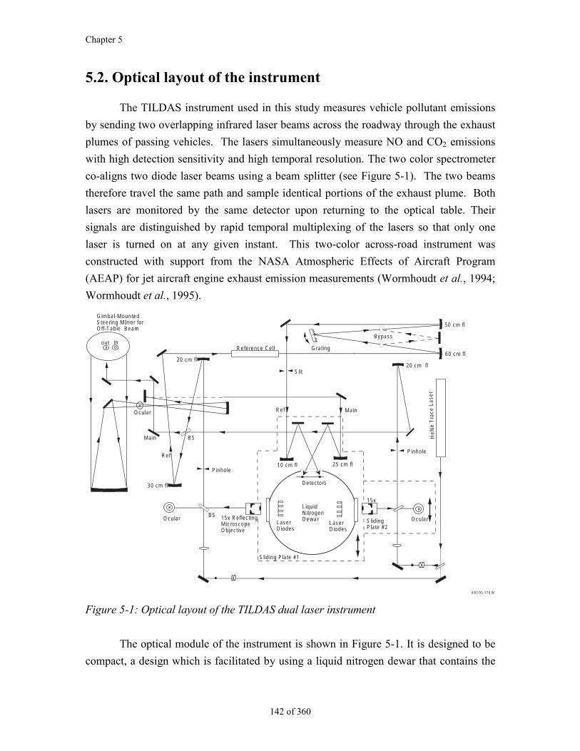
Chapter 5

142 of 360

5.2. Optical layout of the instrument

The TILDAS instrument used in this study measures vehicle pollutant emissions

by sending two overlapping infrared laser beams across the roadway through the exhaust

plumes of passing vehicles. The lasers simultaneously measure NO and CO2 emissions

with high detection sensitivity and high temporal resolution. The two color spectrometer

co-aligns two diode laser beams using a beam splitter (see Figure 5-1). The two beams

therefore travel the same path and sample identical portions of the exhaust plume. Both

lasers are monitored by the same detector upon returning to the optical table. Their

signals are distinguished by rapid temporal multiplexing of the lasers so that only one

laser is turned on at any given instant. This two-color across-road instrument was

constructed with support from the NASA Atmospheric Effects of Aircraft Program

(AEAP) for jet aircraft engine exhaust emission measurements (Wormhoudt et al., 1994;

Wormhoudt et al., 1995).

xout in

Gimbal-Mounted Steering MIrror for Off-Table Beam

x

Ocular

Pinhole

Reference Cell

20 cm fl

Bypass

Grating60 cm fl

Ref Main

HeN

e T

race

Las

er

Slit

30 cm fl

Ref

Main BS

BSLaserDiodes

LaserDiodes

LiquidNitrogenDewar

Pinhole

Detectors

xOcular

15x

Sliding Plate #2

15x

20 cm fl

x

10 cm fl 25 cm fl

ARI-95-17/JW

Ocular15x ReflectingMicroscopeObjective

Sliding Plate #1

50 cm fl

Figure 5-1: Optical layout of the TILDAS dual laser instrument

The optical module of the instrument is shown in Figure 5-1. It is designed to be

compact, a design which is facilitated by using a liquid nitrogen dewar that contains the

The TILDAS Remote Sensor

143 of 360

two laser diodes and the two detector diodes. This dewar offers an excellent alternative to

systems with separate detector dewars and helium refrigerator cold heads, especially for

field applications.

Infrared light from each of the laser diodes in the dewar is collected by a

reflective microscope objective (15x) and focused onto a 200 micron pinhole, which

defines the input aperture. This pinhole is used only during alignment, so it is mounted

on a removable, kinematically indexed base. The microscope objective is mounted on an

X-Y-Z translator to allow accurate focusing into the fixed aperture. Past the input

apertures, the two infrared beams are collimated and combined on the main beam splitter.

One leg of the beam splitter (the “reference leg”) is directed through a gas calibration cell

and onto a detector. Light passing through this cell has strong absorption features that are

used to identify and lock the spectral line positions. The reference leg also passes through

a grating monochromator before being focused onto the detector. The monochromator is

useful for identifying the wavelength of the diode during setup of the instrument.

The “signal leg” is directed to a pair of flat mirrors and onto a large gimbal-

mounted steering mirror which directs the beam off the table and across the roadway to a

corner cube retroreflector. The return beam is collected by the large steering mirror and a

curved mirror of similar diameter, passed through several more flat mirrors and finally

focused onto the signal beam detector. An ocular can be dropped into the path of the

return beam allowing one to observe and optimize the aiming of the outgoing signal

beam. While viewing through this ocular the operator can simultaneously adjust the

gimbal-mounted steering mirror to place the image of the corner cube over the ocular’s

cross hairs. Under many conditions, scattered light from the HeNe “trace laser” (see

below) can be seen on the corner cube’s gold surface showing the precise location of the

optical beam at the corner cube.

A parallel visible optical system is employed for alignment and setup. A red

HeNe "trace" laser beam passes through a dichroic beamsplitter and is coaligned with the

infrared beam. Coalignment is guaranteed by focusing the beam through the input

aperture. The trace beam is an indispensable aid for alignment of the optical system. In

addition, the trace beam is used to accurately calibrate the monochromator, via higher

order diffraction. The fourth port of the dichroic beamsplitter can be used to visibly

observe the laser diode. An eyepiece mounted at the position conjugate to the pinhole

forms an effective microscope for viewing the laser diode.

Chapter 5

144 of 360

5.3. Data Processing and Analysis Techniques

Our data acquisition method is an advanced form of sweep integration which is

carried out by a software package developed at Aerodyne Research. This software uses

commercially available data acquisition boards to control and monitor the diode lasers.

The software sweeps the laser frequency over the full infrared transition or group of

transitions, then integrates the area under the transitions using nonlinear least squares

fitting to the known spectral line shapes and positions. We do not generally use

frequency modulation (FM) techniques because we prefer the clear connection between

the direct absorption spectrum and the species’ concentration. This data acquisition

approach is highly flexible and can be used for many different applications.

There are several advantages to this sweep integration approach. First, absolute

species concentrations are returned from the nonlinear least squares fits so that external

calibration is not required. The species concentrations are tied to the absolute

spectroscopic data found in the HITRAN data base (Rothman et al., 1998). Second, the

line shape functions are known from theory and can be precisely calculated, as described

in section 2.1.3. Finally, this detailed understanding of the expected line shapes and

positions allows one to easily monitor complex and overlapping spectral features. We call

this “fingerprint fitting.” This is important because monitoring several transitions for one

species can enhance sensitivity and is sometimes necessary - especially for larger

molecules.126 In addition, fingerprint fitting allows one to monitor multiple species

simultaneously, since we can use overlapping lines, and it even allows one to fit unknown

lines which overlap the desired spectrum as a method of removing background absorption

from unknown species. This feature is particularly useful in the present application to the

analysis of overlapping N2O and CO2 lines at atmospheric pressure.

The details of the data acquisition process can be divided into several tasks which

we will discuss separately:

The software creates a waveform which is used to modulate the frequency of

the laser or lasers.

The output of the infrared detectors are recorded as a function of time and this

data is stored in the computer’s extended memory.

126 E.g. the overlapping CO2 and N2O transitions in Figure 5-4, and the 24 overlapping NO2 transitions inFigure 7-10.

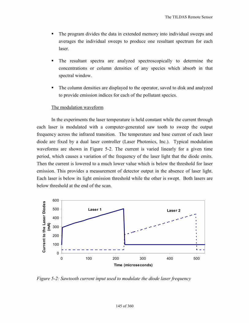
The TILDAS Remote Sensor

145 of 360

The program divides the data in extended memory into individual sweeps and

averages the individual sweeps to produce one resultant spectrum for each

laser.

The resultant spectra are analyzed spectroscopically to determine the

concentrations or column densities of any species which absorb in that

spectral window.

The column densities are displayed to the operator, saved to disk and analyzed

to provide emission indices for each of the pollutant species.

The modulation waveform

In the experiments the laser temperature is held constant while the current through

each laser is modulated with a computer-generated saw tooth to sweep the output

frequency across the infrared transition. The temperature and base current of each laser

diode are fixed by a dual laser controller (Laser Photonics, Inc.). Typical modulation

waveforms are shown in Figure 5-2. The current is varied linearly for a given time

period, which causes a variation of the frequency of the laser light that the diode emits.

Then the current is lowered to a much lower value which is below the threshold for laser

emission. This provides a measurement of detector output in the absence of laser light.

Each laser is below its light emission threshold while the other is swept. Both lasers are

below threshold at the end of the scan.

0

100

200

300

400

500

600

0 100 200 300 400 500

Time (microseconds)

Cu

rre

nt

to t

he

La

se

r D

iod

es

(m

A)

Laser 1 Laser 2

Figure 5-2: Sawtooth current input used to modulate the diode laser frequency

Chapter 5

146 of 360

The digital waveform is converted to an analog voltage at a rate of 300 kHz using

a 12 bit digital to analog converter (Scientific Solutions, Lab Maser AD). Typically 150

points are used to represent the waveforms so that each frequency sweep is 500 µs in

duration.

The infrared detector output

The detector output voltage is sampled by an analog-to digital converter using the

same data acquisition board. The individual spectra are automatically transferred to the

computer’s extended memory using direct memory access.

The averaged spectra

The spectra are coaveraged using assembly language averaging routines in order

to maintain a 100% duty cycle. For automotive exhaust measurements, the averaging

time is typically set to about 10 ms in order to be able to resolve temporal structure in the

exhaust plume (as determined in section 4.2.2). The measurement cycle is triggered by a

vehicle blocking the optical path. Usually, the laser beam height is chosen to be about 29

cm which is a typical tailpipe height. In fact, the measurement process actually begins

before the vehicle blocks the laser beams since the instrument acquires background

spectra continuously while waiting for the next vehicle. The exhaust plume spectra are

each divided by the most recent background spectrum in order to eliminate the effects of

background absorption and to improve sensitivity. This is especially important for

carbon dioxide whose background column density in a 20 meter path (~7,000 ppm-

meters) is nearly as large as the initial column density observed in the exhaust plume with

optimal overlap of laser and plume (~13,000 ppm-meters).

A pair of background corrected spectra are shown in Figure 5-4. We obtained

these spectra during field experiments in the Los Angeles area (see Chapter 6). These

spectra were obtained during the 12.5 ms time slice corresponding to maximum

absorption for a plume with an NO concentration of 1400 ppm and an N2O concentration

of 240 ppm. The scan time for each laser was 250 µs, therefore, the laser scans were

essentially simultaneous. Twenty-five scans of each laser were co-averaged to give a

column density for each species every 12.5 ms. Nitric oxide was measured by recording

the change in absorption of individual rotational-vibrational lines at a frequency around

1903 cm-1 (5.25 µm). The diode laser was scanned over a spectral region of 1cm-1 by

varying the laser current in order to obtain a baseline on either side of a pair of spectral

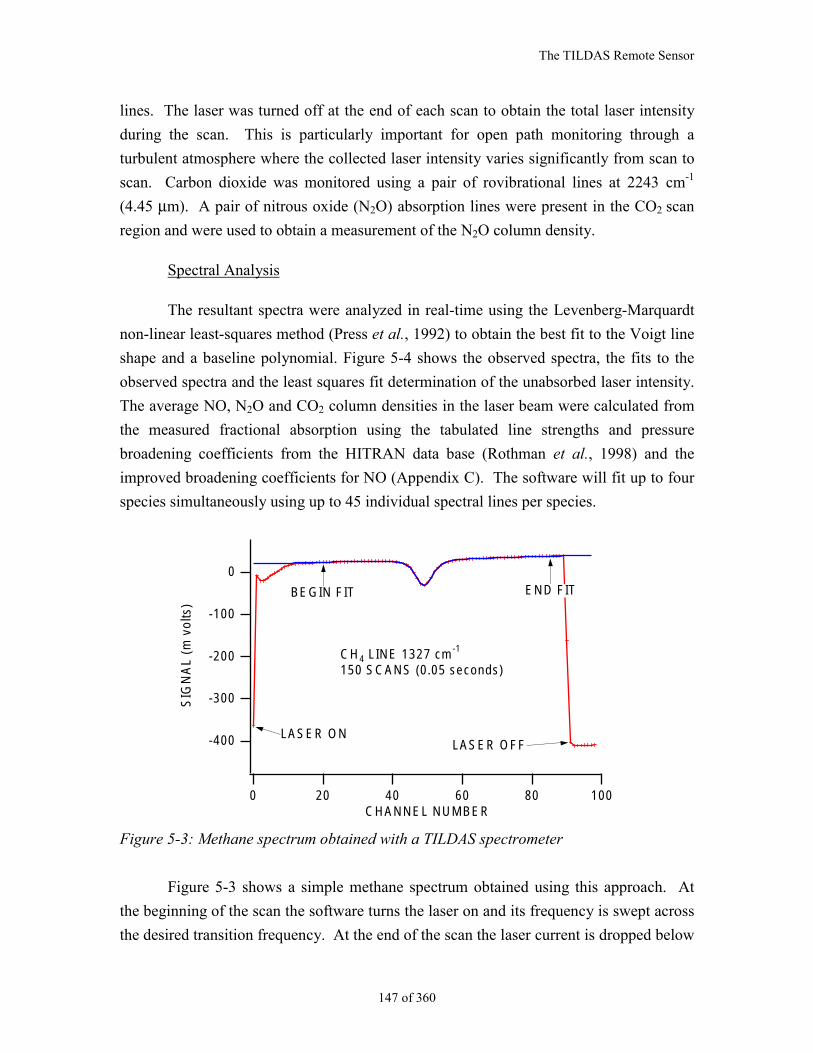
The TILDAS Remote Sensor

147 of 360

lines. The laser was turned off at the end of each scan to obtain the total laser intensity

during the scan. This is particularly important for open path monitoring through a

turbulent atmosphere where the collected laser intensity varies significantly from scan to

scan. Carbon dioxide was monitored using a pair of rovibrational lines at 2243 cm-1

(4.45 µm). A pair of nitrous oxide (N2O) absorption lines were present in the CO2 scan

region and were used to obtain a measurement of the N2O column density.

Spectral Analysis

The resultant spectra were analyzed in real-time using the Levenberg-Marquardt

non-linear least-squares method (Press et al., 1992) to obtain the best fit to the Voigt line

shape and a baseline polynomial. Figure 5-4 shows the observed spectra, the fits to the

observed spectra and the least squares fit determination of the unabsorbed laser intensity.

The average NO, N2O and CO2 column densities in the laser beam were calculated from

the measured fractional absorption using the tabulated line strengths and pressure

broadening coefficients from the HITRAN data base (Rothman et al., 1998) and the

improved broadening coefficients for NO (Appendix C). The software will fit up to four

species simultaneously using up to 45 individual spectral lines per species.

-400

-300

-200

-100

0

SIG

NA

L (m

vol

ts)

100806040200CHANNEL NUMBER

LASER OFFLASER ON

BEGIN FIT END FIT

CH4 LINE 1327 cm-1

150 SCANS (0.05 seconds)

Figure 5-3: Methane spectrum obtained with a TILDAS spectrometer

Figure 5-3 shows a simple methane spectrum obtained using this approach. At

the beginning of the scan the software turns the laser on and its frequency is swept across

the desired transition frequency. At the end of the scan the laser current is dropped below

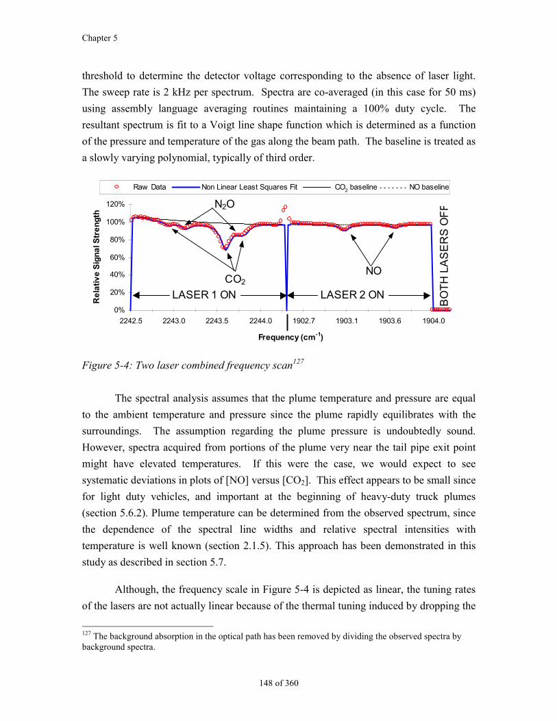
Chapter 5

148 of 360

threshold to determine the detector voltage corresponding to the absence of laser light.

The sweep rate is 2 kHz per spectrum. Spectra are co-averaged (in this case for 50 ms)

using assembly language averaging routines maintaining a 100% duty cycle. The

resultant spectrum is fit to a Voigt line shape function which is determined as a function

of the pressure and temperature of the gas along the beam path. The baseline is treated as

a slowly varying polynomial, typically of third order.

0%

20%

40%

60%

80%

100%

120%

2242.5 2243.0 2243.5 2244.0 1902.7 1903.1 1903.6 1904.0

Frequency (cm-1)

Re

lati

ve

Sig

na

l Str

en

gth

Raw Data Non Linear Least Squares Fit NO baseline

LASER 1 ON LASER 2 ON

CO2NO

N2O

BO

TH

LA

SE

RS

OF

F

CO2 baseline

Figure 5-4: Two laser combined frequency scan127

The spectral analysis assumes that the plume temperature and pressure are equal

to the ambient temperature and pressure since the plume rapidly equilibrates with the

surroundings. The assumption regarding the plume pressure is undoubtedly sound.

However, spectra acquired from portions of the plume very near the tail pipe exit point

might have elevated temperatures. If this were the case, we would expect to see

systematic deviations in plots of [NO] versus [CO2]. This effect appears to be small since

for light duty vehicles, and important at the beginning of heavy-duty truck plumes

(section 5.6.2). Plume temperature can be determined from the observed spectrum, since

the dependence of the spectral line widths and relative spectral intensities with

temperature is well known (section 2.1.5). This approach has been demonstrated in this

study as described in section 5.7.

Although, the frequency scale in Figure 5-4 is depicted as linear, the tuning rates

of the lasers are not actually linear because of the thermal tuning induced by dropping the

127 The background absorption in the optical path has been removed by dividing the observed spectra bybackground spectra.

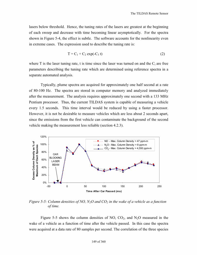
The TILDAS Remote Sensor

149 of 360

lasers below threshold. Hence, the tuning rates of the lasers are greatest at the beginning

of each sweep and decrease with time becoming linear asymptotically. For the spectra

shown in Figure 5-4, the effect is subtle. The software accounts for the nonlinearity even

in extreme cases. The expression used to describe the tuning rate is:

T = C1 + C2 exp(-C3 t) (2)

where T is the laser tuning rate, t is time since the laser was turned on and the Ci are free

parameters describing the tuning rate which are determined using reference spectra in a

separate automated analysis.

Typically, plume spectra are acquired for approximately one half second at a rate

of 80-100 Hz. The spectra are stored in computer memory and analyzed immediately

after the measurement. The analysis requires approximately one second with a 133 MHz

Pentium processor. Thus, the current TILDAS system is capable of measuring a vehicle

every 1.5 seconds. This time interval would be reduced by using a faster processor.

However, it is not be desirable to measure vehicles which are less about 2 seconds apart,

since the emissions from the first vehicle can contaminate the background of the second

vehicle making the measurement less reliable (section 4.2.3).

0%

20%

40%

60%

80%

100%

120%

-50 0 50 100 150 200 250

Time After Car Passed (ms)

Exc

ess

Co

lum

n D

ensi

ty a

s %

of

Max

imu

m o

f E

ach

Sp

ecie

s

NO - Max. Column Density = 47 ppm-m

CAR BLOCKING

LASER BEAM

N2O - Max. Column Density = 8 ppm-mCO2 - Max. Column Density = 4,550 ppm-m

Figure 5-5: Column densities of NO, N2O and CO2 in the wake of a vehicle as a functionof time.

Figure 5-5 shows the column densities of NO, CO2, and N2O measured in the

wake of a vehicle as a function of time after the vehicle passed. In this case the spectra

were acquired at a data rate of 80 samples per second. The correlation of the three species

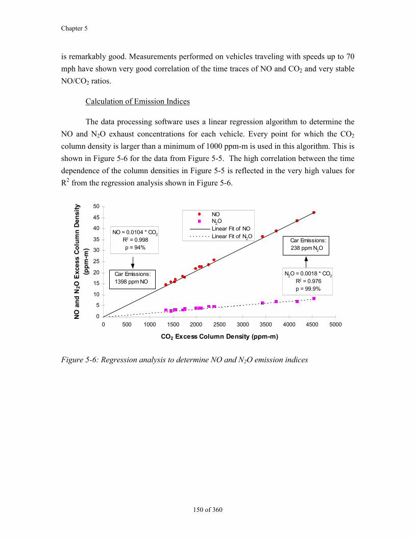
Chapter 5

150 of 360

is remarkably good. Measurements performed on vehicles traveling with speeds up to 70

mph have shown very good correlation of the time traces of NO and CO2 and very stable

NO/CO2 ratios.

Calculation of Emission Indices

The data processing software uses a linear regression algorithm to determine the

NO and N2O exhaust concentrations for each vehicle. Every point for which the CO2

column density is larger than a minimum of 1000 ppm-m is used in this algorithm. This is

shown in Figure 5-6 for the data from Figure 5-5. The high correlation between the time

dependence of the column densities in Figure 5-5 is reflected in the very high values for

R2 from the regression analysis shown in Figure 5-6.

NO = 0.0104 * CO2

R2 = 0.998p = 94%

N2O = 0.0018 * CO2

R2 = 0.976p = 99.9%

0

5

10

15

20

25

30

35

40

45

50

0 500 1000 1500 2000 2500 3000 3500 4000 4500 5000

CO2 Excess Column Density (ppm-m)

NO

an

d N

2O E

xces

s C

olu

mn

Den

sity

(p

pm

-m)

NO

Linear Fit of NO

Car Emissions: 1398 ppm NO

Car Emissions:238 ppm N2O

Linear Fit of N2O

N2O

Figure 5-6: Regression analysis to determine NO and N2O emission indices

The TILDAS Remote Sensor

151 of 360

5.4. Sensitivity and Accuracy of the TILDAS Remote Sensor

5.4.1. Estimation of the instrumental precision in the field

The TILDAS instrument detection limit for NO has been estimated from the noise

levels observed during open path field tests performed in the absence of a vehicle. Each

measurement was performed for 100 ms to simulate the plume duration of actual on-road

exhaust measurements. The observed NO column densities were converted to exhaust

mixing ratios using a value of the CO2 column density (13,000 ppm-meters) which

corresponds to ideal overlap of laser beam and exhaust plume. These tests returned an

NO column density near zero with a standard deviation equivalent to an exhaust mixing

ratio of ~3 ppm. We therefore report the ideal 3σ detection limit as ~9 ppm NO.

Experimental confirmation of this detection limit has been obtained by repeated

measurements on an ultra low emission vehicle (ULEV) as is described below. The

result for N2O was 2 ppm, or ~6 ppm for the ideal 3σ detection limit.

This level of sensitivity is the best that has been demonstrated for any NO remote

sensor, with an improvement in the detection limit by a factor of approximately 100 over

the two widely employed commercial techniques (Jack et al., 1995; Zhang et al., 1996a),

and by a factor of 4 to 7 over the most precise UV instrument (Jack et al., 1995; Zhang et

al., 1996a; Popp et al., 1997).

This high sensitivity enables the TILDAS technique to measure the NO emissions

from even the cleanest vehicles on the road. For example, average signal-to-noise ratios

(SNR) of the NO measurement for an ultra-low emissions vehicle (ULEV)128 would be

about 28, when generally a SNR of 3 is the minimum for a good measurement. A vehicle

complying with the most stringent regulation ever proposed for light-duty vehicle NOx,

California’s proposed Super Ultra Low Emission Vehicle regulation (SULEV, as defined

in CARB, 1998c), would still be marginally measurable with TILDAS (SNR of 3).129

128 ULEV is a California emission standard. A fuel economy of 30 mpg has been assumed.129 Assuming a fuel economy of 30 mpg.

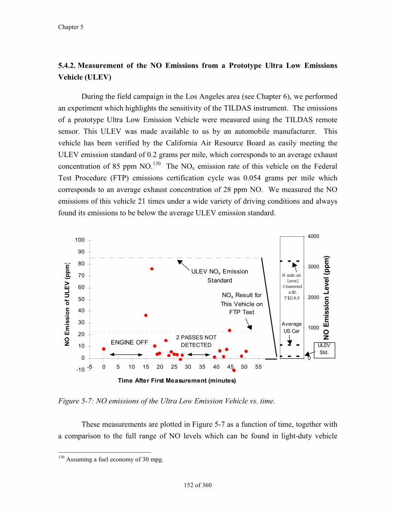
Chapter 5

152 of 360

5.4.2. Measurement of the NO Emissions from a Prototype Ultra Low Emissions

Vehicle (ULEV)

During the field campaign in the Los Angeles area (see Chapter 6), we performed

an experiment which highlights the sensitivity of the TILDAS instrument. The emissions

of a prototype Ultra Low Emission Vehicle were measured using the TILDAS remote

sensor. This ULEV was made available to us by an automobile manufacturer. This

vehicle has been verified by the California Air Resource Board as easily meeting the

ULEV emission standard of 0.2 grams per mile, which corresponds to an average exhaust

concentration of 85 ppm NO.130 The NOx emission rate of this vehicle on the Federal

Test Procedure (FTP) emissions certification cycle was 0.054 grams per mile which

corresponds to an average exhaust concentration of 28 ppm NO. We measured the NO

emissions of this vehicle 21 times under a wide variety of driving conditions and always

found its emissions to be below the average ULEV emission standard.

-10

0

10

20

30

40

50

60

70

80

90

100

-5 0 5 10 15 20 25 30 35 40 45 50 55

Time After First Measurement (minutes)

NO

Em

issi

on

of

UL

EV

(p

pm

)

ENGINE OFF

ULEV NOx Emission

Standard

NOx Result for

This Vehicle on FTP Test

2 PASSES NOT DETECTED

0

1000

2000

3000

4000

NO

Em

issi

on

Lev

el (

pp

m)

M axim um Level

Observed with

TILDAS

Average US Car

ULEVStd.

Figure 5-7: NO emissions of the Ultra Low Emission Vehicle vs. time.

These measurements are plotted in Figure 5-7 as a function of time, together with

a comparison to the full range of NO levels which can be found in light-duty vehicle

130 Assuming a fuel economy of 30 mpg.

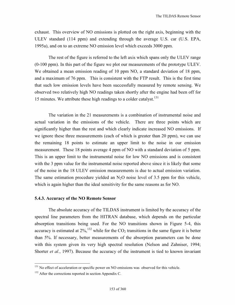
The TILDAS Remote Sensor

153 of 360

exhaust. This overview of NO emissions is plotted on the right axis, beginning with the

ULEV standard (114 ppm) and extending through the average U.S. car (U.S. EPA,

1995a), and on to an extreme NO emission level which exceeds 3000 ppm.

The rest of the figure is referred to the left axis which spans only the ULEV range

(0-100 ppm). In this part of the figure we plot our measurements of the prototype ULEV.

We obtained a mean emission reading of 10 ppm NO, a standard deviation of 18 ppm,

and a maximum of 76 ppm. This is consistent with the FTP result. This is the first time

that such low emission levels have been successfully measured by remote sensing. We

observed two relatively high NO readings taken shortly after the engine had been off for

15 minutes. We attribute these high readings to a colder catalyst.131

The variation in the 21 measurements is a combination of instrumental noise and

actual variation in the emissions of the vehicle. There are three points which are

significantly higher than the rest and which clearly indicate increased NO emissions. If

we ignore these three measurements (each of which is greater than 20 ppm), we can use

the remaining 18 points to estimate an upper limit to the noise in our emission

measurement. These 18 points average 4 ppm of NO with a standard deviation of 5 ppm.

This is an upper limit to the instrumental noise for low NO emissions and is consistent

with the 3 ppm value for the instrumental noise reported above since it is likely that some

of the noise in the 18 ULEV emission measurements is due to actual emission variation.

The same estimation procedure yielded an N2O noise level of 3.5 ppm for this vehicle,

which is again higher than the ideal sensitivity for the same reasons as for NO.

5.4.3. Accuracy of the NO Remote Sensor

The absolute accuracy of the TILDAS instrument is limited by the accuracy of the

spectral line parameters from the HITRAN database, which depends on the particular

absorption transitions being used. For the NO transitions shown in Figure 5-4, this

accuracy is estimated at 2%,132 while for the CO2 transitions in the same figure it is better

than 5%. If necessary, better measurements of the absorption parameters can be done

with this system given its very high spectral resolution (Nelson and Zahniser, 1994;

Shorter et al., 1997). Because the accuracy of the instrument is tied to known invariant

131 No effect of acceleration or specific power on NO emissions was observed for this vehicle.132 After the corrections reported in section Appendix C.

Chapter 5

154 of 360

physical properties, it does not need periodic calibrations. This is a significant advantage

for field measurements using the TILDAS technique.

This accuracy was verified by comparing the TILDAS NOx/CO2 measurements

with those of the on-board instrumentation of the EPA heavy-duty diesel truck, as shown

in Figure 7-5. The average of the TILDAS measurements was 99% ± 4.7%, which

indicates that the TILDAS instrument is accurate within the experimental uncertainty.

The precision of these measurements is not as good as the one reported in sections

5.4.1 and 5.4.2 for two main reasons:

Variation of the emission ratios of the EPA instrumented truck within the same

measurement.

The fact that remote sensing precision is lower for any technique when measuring

high pollutant concentrations, as explained in section 4.4.

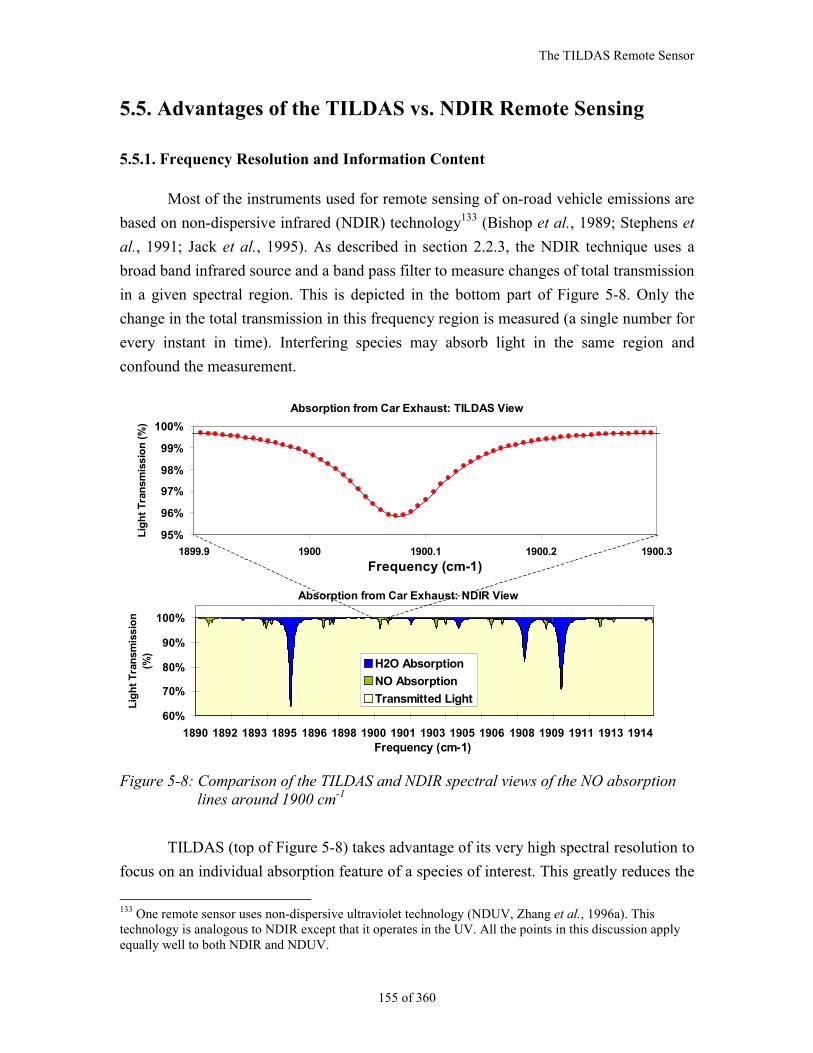
The TILDAS Remote Sensor

155 of 360

5.5. Advantages of the TILDAS vs. NDIR Remote Sensing

5.5.1. Frequency Resolution and Information Content

Most of the instruments used for remote sensing of on-road vehicle emissions are

based on non-dispersive infrared (NDIR) technology133 (Bishop et al., 1989; Stephens et

al., 1991; Jack et al., 1995). As described in section 2.2.3, the NDIR technique uses a

broad band infrared source and a band pass filter to measure changes of total transmission

in a given spectral region. This is depicted in the bottom part of Figure 5-8. Only the

change in the total transmission in this frequency region is measured (a single number for

every instant in time). Interfering species may absorb light in the same region and

confound the measurement.

Absorption from Car Exhaust: NDIR View

60%

70%

80%

90%

100%

1890 1892 1893 1895 1896 1898 1900 1901 1903 1905 1906 1908 1909 1911 1913 1914Frequency (cm-1)

Lig

ht

Tra

nsm

issi

on

(%

)

H2O Absorption

NO Absorption

Transmitted Light

Absorption from Car Exhaust: TILDAS View

95%

96%

97%

98%

99%

100%

1899.9 1900 1900.1 1900.2 1900.3

Frequency (cm-1)

Lig

ht

Tra

nsm

issi

on

(%

)

Figure 5-8: Comparison of the TILDAS and NDIR spectral views of the NO absorptionlines around 1900 cm-1

TILDAS (top of Figure 5-8) takes advantage of its very high spectral resolution to

focus on an individual absorption feature of a species of interest. This greatly reduces the

133 One remote sensor uses non-dispersive ultraviolet technology (NDUV, Zhang et al., 1996a). Thistechnology is analogous to NDIR except that it operates in the UV. All the points in this discussion applyequally well to both NDIR and NDUV.

Chapter 5

156 of 360

possibility of interference from other chemical species. An additional advantage is that

TILDAS provides much more information in each measurement than NDIR does: dozens

of transmission vs. frequency data points versus only one total transmission for the whole

filtered spectral region. For both of these reasons TILDAS is able to achieve greater

precision than NDIR is (5 ppm vs. 300 ppm for NO, respectively).

A new NO remote sensor based on ultraviolet (UV) spectroscopy (Popp et al.,

1997) achieved much higher precision134 than its NDUV predecessor (Zhang et al.,

1996a) by using a technique conceptually similar to TILDAS. In this instrument the UV

beam is diffracted in a grating and sent to an array of detectors so a curve of transmission

vs. frequency is obtained. This approach shares part of the two main advantages of

TILDAS: the effect of interferences can be greatly reduced and the amount of

information in each measurement is increased.

5.5.2. Long Optical Path

A long pathlength is of interest for remote sensing since it would allow greater

flexibility in the placement of the sensors (e.g. across multilane highways). Some studies

also suggest that drivers change their behavior while driving in front of a remote sensor.

Walsh and Gertler (Walsh et al., 1997) found that for those light-duty vehicles with one

high and one low remote sensing measurement, the first measurement was the high one

on 60% of the cases. They suggest that motorists may have been aware of the remote

sensing device after the first pass and may have altered their driving in response. A

longer pathlength could avoid this problem since the instrument would be less visible. It

would also diminish associated concerns of motorist and operator safety which greatly

limit site selection (Walsh et al., 1997), and vandalism of unmanned remote sensors.

NDIR-based instruments are very limited in this respect due to the angular

dispersion of their non-laser light, and because the absorption due to background CO2

decreases the signal-to-noise ratio of their CO2 measurement (HES, 1992). The longest

pathlengths reported with this type of instruments are 40 to 50 ft (12m) (HES, 1992;

Stedman et al., 1994). Bishop and Stedman (Bishop et al., 1996c) report in a recent

description of their NDIR-UV instrument that “the system is designed to operate on a

single lane road. […] Multiple lane operation has been reported but is not

recommended.”

134 About 20 ppm NO vs. 300 ppm NO.

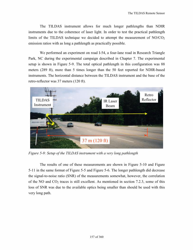
The TILDAS Remote Sensor

157 of 360

The TILDAS instrument allows for much longer pathlengths than NDIR

instruments due to the coherence of laser light. In order to test the practical pathlength

limits of the TILDAS technique we decided to attempt the measurement of NO/CO2

emission ratios with as long a pathlength as practically possible.

We performed an experiment on road I-54, a four-lane road in Research Triangle

Park, NC during the experimental campaign described in Chapter 7. The experimental

setup is shown in Figure 5-9. The total optical pathlength in this configuration was 88

meters (289 ft), more than 5 times longer than the 50 feet reported for NDIR-based

instruments. The horizontal distance between the TILDAS instrument and the base of the

retro-reflector was 37 meters (120 ft).

RetroReflectorTILDAS

InstrumentIR Laser

Beam

37 m (120 ft)

Figure 5-9: Setup of the TILDAS instrument with a very long pathlength

The results of one of these measurements are shown in Figure 5-10 and Figure

5-11 in the same format of Figure 5-5 and Figure 5-6. The longer pathlength did decrease

the signal-to-noise ratio (SNR) of the measurements somewhat, however, the correlation

of the NO and CO2 traces is still excellent. As mentioned in section 7.2.3, some of this

loss of SNR was due to the available optics being smaller than should be used with this

very long path.

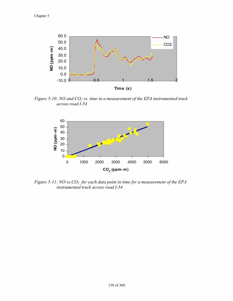
Chapter 5

158 of 360

-10.0

0.0

10.0

20.0

30.0

40.0

50.0

60.0

0 0.5 1 1.5 2

Time (s)

NO

(p

pm-m

)

NO

CO2

Figure 5-10: NO and CO2 vs. time in a measurement of the EPA instrumented truckacross road I-54

0

10

20

30

40

50

60

0 1000 2000 3000 4000 5000 6000

CO2 (ppm-m)

NO

(p

pm

-m)

Figure 5-11: NO vs.CO2 for each data point in time for a measurement of the EPAinstrumented truck across road I-54

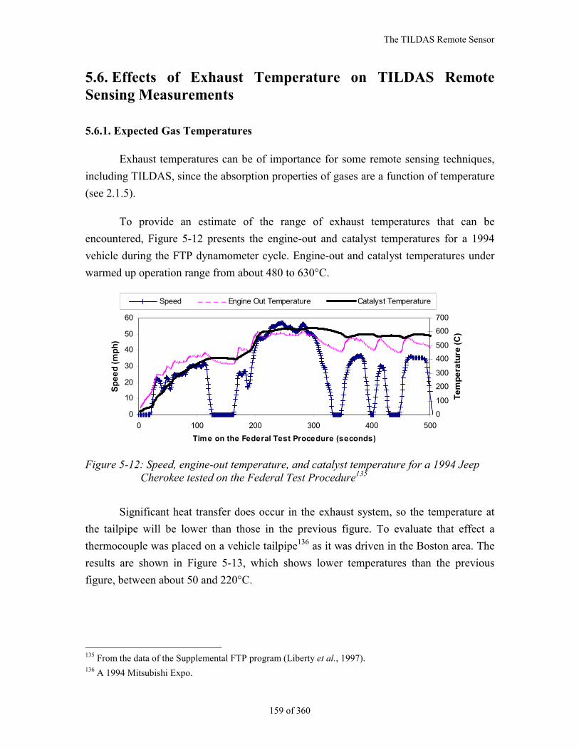
The TILDAS Remote Sensor

159 of 360

5.6. Effects of Exhaust Temperature on TILDAS RemoteSensing Measurements

5.6.1. Expected Gas Temperatures

Exhaust temperatures can be of importance for some remote sensing techniques,

including TILDAS, since the absorption properties of gases are a function of temperature

(see 2.1.5).

To provide an estimate of the range of exhaust temperatures that can be

encountered, Figure 5-12 presents the engine-out and catalyst temperatures for a 1994

vehicle during the FTP dynamometer cycle. Engine-out and catalyst temperatures under

warmed up operation range from about 480 to 630°C.

0

10

20

30

40

50

60

0 100 200 300 400 500

Time on the Federal Test Procedure (seconds)

Sp

ee

d (

mp

h)

0

100

200

300

400

500

600

700

Te

mp

era

ture

(C

)

Speed Engine Out Temperature Catalyst Temperature

Figure 5-12: Speed, engine-out temperature, and catalyst temperature for a 1994 JeepCherokee tested on the Federal Test Procedure135

Significant heat transfer does occur in the exhaust system, so the temperature at

the tailpipe will be lower than those in the previous figure. To evaluate that effect a

thermocouple was placed on a vehicle tailpipe136 as it was driven in the Boston area. The

results are shown in Figure 5-13, which shows lower temperatures than the previous

figure, between about 50 and 220°C.

135 From the data of the Supplemental FTP program (Liberty et al., 1997).136 A 1994 Mitsubishi Expo.

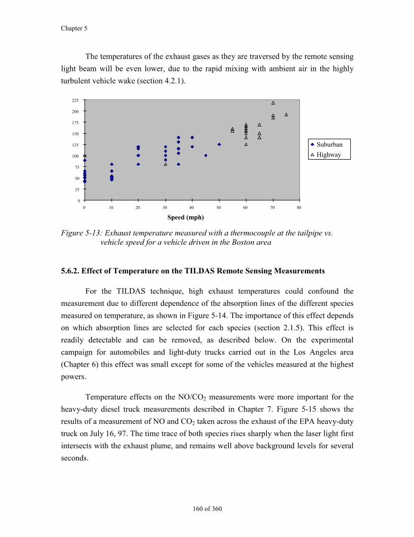
Chapter 5

160 of 360

The temperatures of the exhaust gases as they are traversed by the remote sensing

light beam will be even lower, due to the rapid mixing with ambient air in the highly

turbulent vehicle wake (section 4.2.1).

0

25

50

75

100

125

150

175

200

225

0 10 20 30 40 50 60 70 80

Speed (mph)

Suburban

Highway

Figure 5-13: Exhaust temperature measured with a thermocouple at the tailpipe vs.vehicle speed for a vehicle driven in the Boston area

5.6.2. Effect of Temperature on the TILDAS Remote Sensing Measurements

For the TILDAS technique, high exhaust temperatures could confound the

measurement due to different dependence of the absorption lines of the different species

measured on temperature, as shown in Figure 5-14. The importance of this effect depends

on which absorption lines are selected for each species (section 2.1.5). This effect is

readily detectable and can be removed, as described below. On the experimental

campaign for automobiles and light-duty trucks carried out in the Los Angeles area

(Chapter 6) this effect was small except for some of the vehicles measured at the highest

powers.

Temperature effects on the NO/CO2 measurements were more important for the

heavy-duty diesel truck measurements described in Chapter 7. Figure 5-15 shows the

results of a measurement of NO and CO2 taken across the exhaust of the EPA heavy-duty

truck on July 16, 97. The time trace of both species rises sharply when the laser light first

intersects with the exhaust plume, and remains well above background levels for several

seconds.

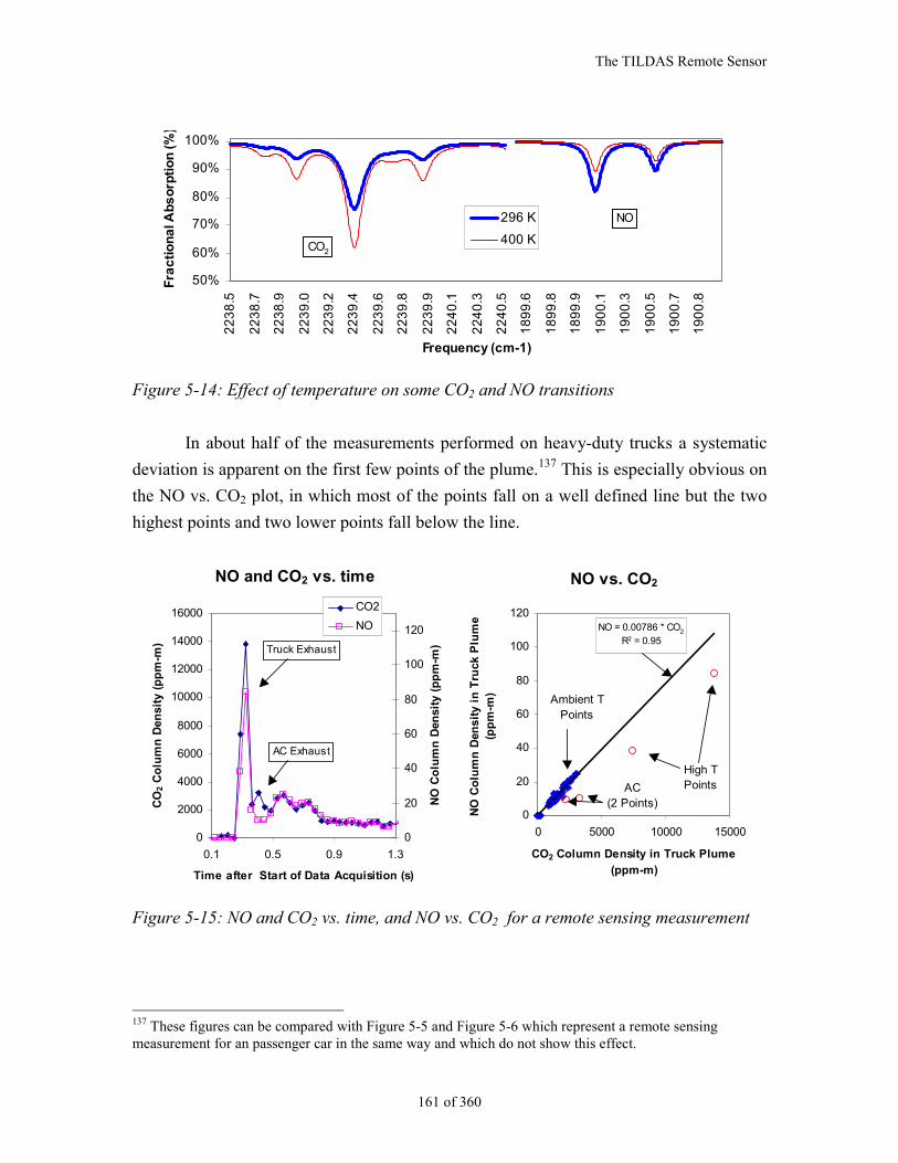
The TILDAS Remote Sensor

161 of 360

50%

60%

70%

80%

90%

100%

22

38

.5

22

38

.7

22

38

.9

22

39

.0

22

39

.2

22

39

.4

22

39

.6

22

39

.8

22

39

.9

22

40

.1

22

40

.3

22

40

.5

18

99

.6

18

99

.8

18

99

.9

19

00

.1

19

00

.3

19

00

.5

19

00

.7

19

00

.8

Frequency (cm-1)

Fra

cti

on

al A

bs

orp

tio

n (

%)

296 K

400 KCO2

NO

Figure 5-14: Effect of temperature on some CO2 and NO transitions

In about half of the measurements performed on heavy-duty trucks a systematic

deviation is apparent on the first few points of the plume.137 This is especially obvious on

the NO vs. CO2 plot, in which most of the points fall on a well defined line but the two

highest points and two lower points fall below the line.

NO and CO2 vs. time

0

2000

4000

6000

8000

10000

12000

14000

16000

0.1 0.5 0.9 1.3

Time after Start of Data Acquisition (s)

CO

2 C

olu

mn

Den

sity

(p

pm

-m)

0

20

40

60

80

100

120

NO

Co

lum

n D

ensi

ty (

pp

m-m

)

CO2

NO

AC Exhaust

Truck Exhaust

NO vs. CO2

NO = 0.00786 * CO2

R2 = 0.95

0

20

40

60

80

100

120

0 5000 10000 15000

CO2 Column Density in Truck Plume

(ppm-m)

NO

Co

lum

n D

ensi

ty i

n T

ruck

Plu

me

(pp

m-m

)

High TPoints

Ambient TPoints

AC(2 Points)

Figure 5-15: NO and CO2 vs. time, and NO vs. CO2 for a remote sensing measurement

137 These figures can be compared with Figure 5-5 and Figure 5-6 which represent a remote sensingmeasurement for an passenger car in the same way and which do not show this effect.

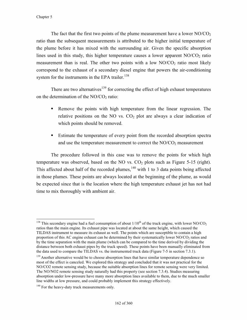
Chapter 5

162 of 360

The fact that the first two points of the plume measurement have a lower NO/CO2

ratio than the subsequent measurements is attributed to the higher initial temperature of

the plume before it has mixed with the surrounding air. Given the specific absorption

lines used in this study, this higher temperature causes a lower apparent NO/CO2 ratio

measurement than is real. The other two points with a low NO/CO2 ratio most likely

correspond to the exhaust of a secondary diesel engine that powers the air-conditioning

system for the instruments in the EPA trailer.138

There are two alternatives139 for correcting the effect of high exhaust temperatures

on the determination of the NO/CO2 ratio:

Remove the points with high temperature from the linear regression. The

relative positions on the NO vs. CO2 plot are always a clear indication of

which points should be removed.

Estimate the temperature of every point from the recorded absorption spectra

and use the temperature measurement to correct the NO/CO2 measurement

The procedure followed in this case was to remove the points for which high

temperature was observed, based on the NO vs. CO2 plots such as Figure 5-15 (right).

This affected about half of the recorded plumes,140 with 1 to 3 data points being affected

in those plumes. These points are always located at the beginning of the plume, as would

be expected since that is the location where the high temperature exhaust jet has not had

time to mix thoroughly with ambient air.

138 This secondary engine had a fuel consumption of about 1/10th of the truck engine, with lower NO/CO2

ratios than the main engine. Its exhaust pipe was located at about the same height, which caused theTILDAS instrument to measure its exhaust as well. The points which are susceptible to contain a highproportion of this AC engine exhaust can be determined by their systematically lower NO/CO2 ratios andby the time separation with the main plume (which can be compared to the time derived by dividing thedistance between both exhaust pipes by the truck speed). These points have been manually eliminated fromthe data used to compare the TILDAS vs. the instrumented truck data (Figure 7-5 in section 7.3.1).139 Another alternative would be to choose absorption lines that have similar temperature dependence somost of the effect is canceled. We explored this strategy and concluded that it was not practical for theNO/CO2 remote sensing study, because the suitable absorption lines for remote sensing were very limited.The NO/NO2 remote sensing study naturally had this property (see section 7.3.4). Studies measuringabsorption under low-pressure have many more absorption lines available to them, due to the much smallerline widths at low pressure, and could probably implement this strategy effectively.140 For the heavy-duty truck measurements only.

The TILDAS Remote Sensor

163 of 360

The estimation of gas temperature from its effect on the shape of absorption

spectra has also been successfully achieved for some of the experimental data obtained in

this study. The details of the temperature estimation procedure are given in section 5.7.

Chapter 5

164 of 360

5.7. Determination of Gas Temperature from TILDAS RemoteSensing Spectra

5.7.1. Motivation

It was shown in section 5.6.2 that the effect of high exhaust temperatures can be

important for the NO/CO2 remote sensing measurement, specially for heavy-duty diesel

trucks. This problem can be reliably detected by looking at deviations in the linear

regression fit (Figure 5-15) and those points can be eliminated. That approach has been

implemented in for the data presented here.

However, a more direct approach would be to determine the gas temperature141

from the recorded spectra, since both line strength and line width are known functions of

temperature. Once gas temperature is known, the data points with elevated temperatures

can be screened out automatically. Alternatively, the temperature measurement can be

used to correct for the temperature effect and the data points can be included in the

regression analysis for determining the NO/CO2 ratio for a given vehicle (Figure 5-15-

right).

5.7.2. Previous Work on Gas Temperature Measurement using Absorption

Spectroscopy

The application of laser techniques to the measurement of temperature and other

scalars has been pioneered by researchers in combustion and supersonic flow diagnostics,

due to these fields’ need for precise, fast, and non-intrusive measurements. Eckbreth

(Eckbreth, 1981) reviews the early efforts of temperature measurement using non-

absorption laser techniques such as Raman scattering, Rayleigh scattering, and laser-

induced fluorescence (LIF).

Temperature measurements in combustion systems using the diode-laser

absorption technique have been pioneered by the Hanson research group at Stanford

University (Chang et al., 1991; Arroyo and Hanson, 1993; Philippe and Hanson, 1993;

Arroyo et al., 1994; Baer et al., 1994; Baer et al., 1996; Nagali et al., 1997; Mihalcea et

141 In this section we use “exhaust temperature” to refer to the temperature of the undiluted exhaust gases asthey leave the vehicle’s tailpipe. “Gas temperature” refers to the temperature of the exhaust as it is beingdiluted with ambient air after leaving the tailpipe.

The TILDAS Remote Sensor

165 of 360

al., 1998), and also pursued by other groups (Allen and Kessler, 1996; Mohamed et al.,

1996). This efforts are summarized in the recent review by Allen (Allen, 1998).

Three basic approaches have been used in those studies in which temperature is

determined:

from the ratio of the integrated absorption of 2 absorption lines (Chang et al., 1991;

Arroyo et al., 1993; Arroyo et al., 1994; Baer et al., 1994; Allen et al., 1996; Baer et

al., 1996; Mihalcea et al., 1998)

from the ratio of peak absorption of 2 absorption lines (Baer et al., 1996; Nagali et

al., 1997)

from a non-linear least-squares fit to the frequency vs. absorption data (Philippe et al.,

1993; Mohamed et al., 1996)

Sensitivities of up to 2 degrees K at ambient temperatures have been reported

with the first technique (Baer et al., 1994). In general the achievable sensitivity will be

different for each combination of diode laser power, detector characteristics, absorption

lines used, measured temperatures, averaging time, and species column density observed.

However, this result indicates that measuring temperature from remote sensing spectra is

feasible in principle.

A variant of the first two approaches was tried in this study but was found to not

give adequate performance. I believe this is due to the uncertainty in the baseline laser

intensity for the pressure broadened absorption lines used in this study. Nagali and

Hanson reported a similar problem which they solved by using an additional laser diode

to determine the baseline intensity (Nagali et al., 1997).

A variant of the third approach was determined to be the most feasible option for

this study for 2 reasons:

Using the full frequency vs. absorption data makes use of the most information

content of the three approaches.

An additional laser channel may allow the use of the peak-absorption ratio technique

of Nagali and Hanson (Nagali et al., 1997). However, such a channel is not available

in the instrument used in this study, and any future channels will be preferentially

devoted to the measurement of additional species rather than exhaust temperature.

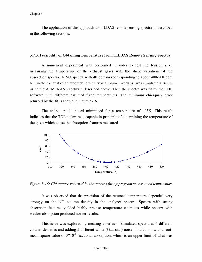
Chapter 5

166 of 360

The application of this approach to TILDAS remote sensing spectra is described

in the following sections.

5.7.3. Feasibility of Obtaining Temperature from TILDAS Remote Sensing Spectra

A numerical experiment was performed in order to test the feasibility of

measuring the temperature of the exhaust gases with the shape variations of the

absorption spectra. A NO spectra with 40 ppm-m (corresponding to about 400-800 ppm

NO in the exhaust of an automobile with typical plume overlaps) was simulated at 400K

using the ATMTRANS software described above. Then the spectra was fit by the TDL

software with different assumed fixed temperatures. The minimum chi-square error

returned by the fit is shown in Figure 5-16.

The chi-square is indeed minimized for a temperature of 403K. This result

indicates that the TDL software is capable in principle of determining the temperature of

the gases which cause the absorption features measured.

0

20

40

60

80

100

300 320 340 360 380 400 420 440 460 480 500

Temperature (K)

Ch

i2

Figure 5-16: Chi-square returned by the spectra fitting program vs. assumed temperature

It was observed that the precision of the returned temperature depended very

strongly on the NO column density in the analyzed spectra. Spectra with strong

absorption features yielded highly precise temperature estimates while spectra with

weaker absorption produced noisier results.

This issue was explored by creating a series of simulated spectra at 6 different

column densities and adding 5 different white (Gaussian) noise simulations with a root-

mean-square value of 3*10-4 fractional absorption, which is an upper limit of what was

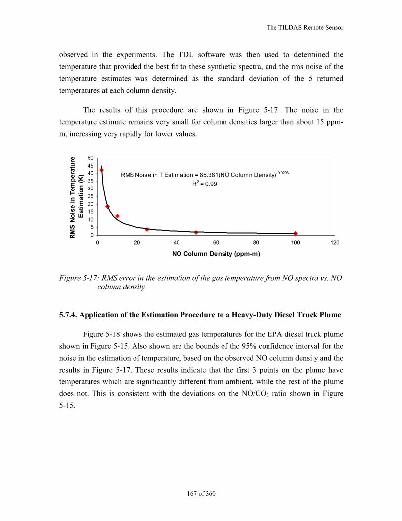
The TILDAS Remote Sensor

167 of 360

observed in the experiments. The TDL software was then used to determined the

temperature that provided the best fit to these synthetic spectra, and the rms noise of the

temperature estimates was determined as the standard deviation of the 5 returned

temperatures at each column density.

The results of this procedure are shown in Figure 5-17. The noise in the

temperature estimate remains very small for column densities larger than about 15 ppm-

m, increasing very rapidly for lower values.

RMS Noise in T Estimation = 85.381(NO Column Density)-0.9298

R2 = 0.99

0

510

1520

25

3035

4045

50

0 20 40 60 80 100 120

NO Column Density (ppm-m)

RM

S N

ois

e in

Tem

per

atu

re

Est

imat

ion

(K

)

Figure 5-17: RMS error in the estimation of the gas temperature from NO spectra vs. NOcolumn density

5.7.4. Application of the Estimation Procedure to a Heavy-Duty Diesel Truck Plume

Figure 5-18 shows the estimated gas temperatures for the EPA diesel truck plume

shown in Figure 5-15. Also shown are the bounds of the 95% confidence interval for the

noise in the estimation of temperature, based on the observed NO column density and the

results in Figure 5-17. These results indicate that the first 3 points on the plume have

temperatures which are significantly different from ambient, while the rest of the plume

does not. This is consistent with the deviations on the NO/CO2 ratio shown in Figure

5-15.

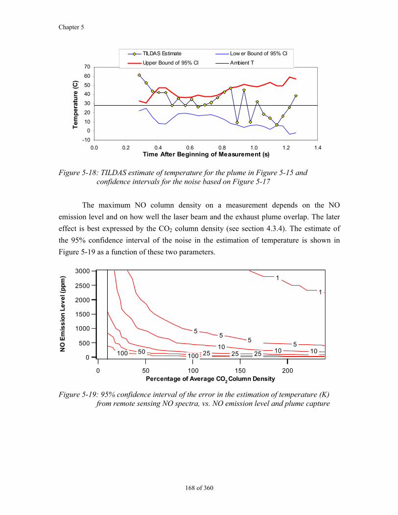
Chapter 5

168 of 360

-10

0

10

20

30

40

50

60

70

0.0 0.2 0.4 0.6 0.8 1.0 1.2 1.4Time After Beginning of Measurement (s)

Tem

per

atu

re (

C)

TILDAS Estimate Low er Bound of 95% CI

Upper Bound of 95% CI Ambient T

Figure 5-18: TILDAS estimate of temperature for the plume in Figure 5-15 andconfidence intervals for the noise based on Figure 5-17

The maximum NO column density on a measurement depends on the NO

emission level and on how well the laser beam and the exhaust plume overlap. The later

effect is best expressed by the CO2 column density (see section 4.3.4). The estimate of

the 95% confidence interval of the noise in the estimation of temperature is shown in

Figure 5-19 as a function of these two parameters.

3000

2500

2000

1500

1000

500

0

NO

Em

iss

ion

Le

ve

l (p

pm

)

200150100500 Percentage of Average CO2 Column Density

100 50 25 25 10 10 10

5 5

5

5

1

1

100 25 100

Figure 5-19: 95% confidence interval of the error in the estimation of temperature (K)from remote sensing NO spectra, vs. NO emission level and plume capture

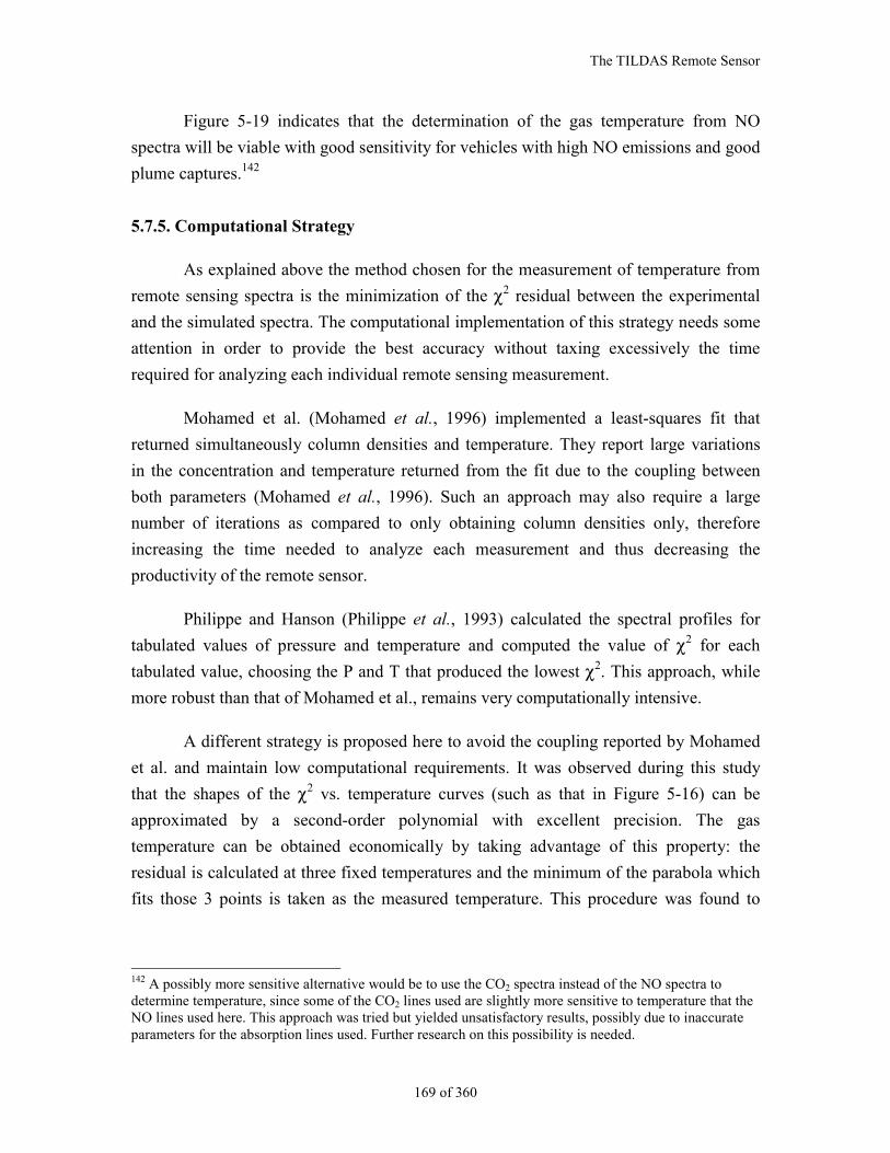
The TILDAS Remote Sensor

169 of 360

Figure 5-19 indicates that the determination of the gas temperature from NO

spectra will be viable with good sensitivity for vehicles with high NO emissions and good

plume captures.142

5.7.5. Computational Strategy

As explained above the method chosen for the measurement of temperature from

remote sensing spectra is the minimization of the χ2 residual between the experimental

and the simulated spectra. The computational implementation of this strategy needs some

attention in order to provide the best accuracy without taxing excessively the time

required for analyzing each individual remote sensing measurement.

Mohamed et al. (Mohamed et al., 1996) implemented a least-squares fit that

returned simultaneously column densities and temperature. They report large variations

in the concentration and temperature returned from the fit due to the coupling between

both parameters (Mohamed et al., 1996). Such an approach may also require a large

number of iterations as compared to only obtaining column densities only, therefore

increasing the time needed to analyze each measurement and thus decreasing the

productivity of the remote sensor.

Philippe and Hanson (Philippe et al., 1993) calculated the spectral profiles for

tabulated values of pressure and temperature and computed the value of χ2 for each

tabulated value, choosing the P and T that produced the lowest χ2. This approach, while

more robust than that of Mohamed et al., remains very computationally intensive.

A different strategy is proposed here to avoid the coupling reported by Mohamed

et al. and maintain low computational requirements. It was observed during this study

that the shapes of the χ2 vs. temperature curves (such as that in Figure 5-16) can be

approximated by a second-order polynomial with excellent precision. The gas

temperature can be obtained economically by taking advantage of this property: the

residual is calculated at three fixed temperatures and the minimum of the parabola which

fits those 3 points is taken as the measured temperature. This procedure was found to

142 A possibly more sensitive alternative would be to use the CO2 spectra instead of the NO spectra todetermine temperature, since some of the CO2 lines used are slightly more sensitive to temperature that theNO lines used here. This approach was tried but yielded unsatisfactory results, possibly due to inaccurateparameters for the absorption lines used. Further research on this possibility is needed.

Chapter 5

170 of 360

consistently return temperatures within a few K of the true minimum, and only requires

running the fitting program 4 times.

The TILDAS Remote Sensor

171 of 360

5.8. Conclusions on TILDAS Remote Sensing

A TILDAS instrument has been modified for use as a remote sensor of vehicle

emissions. The current instrument operates two diode lasers in two different frequency

regions. The sensitivity of the instrument is 3 ppm NO and 2 ppm N2O under ideal

conditions. This has been demonstrated by measurements on an Ultra Low Emission

vehicle.

The main advantages of the TILDAS technique for its application to remote

sensing of vehicle emissions are:

The high sensitivity of the technique, which allows the measurement of the emissions

from even the cleanest vehicles.

The unique ability of this technique to remotely sense minor species of interest in

automotive exhaust such as NO2, NH3, N2O, and formaldehyde.

The absence of interferences from other gases or particulates in the vehicle exhaust or

in ambient air, or from infrared emission from the vehicle or the exhaust, due to the

its very high spectral resolution and fast time response.

The higher information content of the technique with respect to NDIR or NDUV

make it more robust against anoumalous effects such as interferences from the

exhaust of previous vehicles, vibrations, etc.

The absolute nature of this technique, which makes repeated calibrations unnecessary.

Other techniques require frequent field calibration to resist inherent drifts.

The longer path length achievable with this technique with only minor degradation of

sensitivity, due to the coherent nature of laser radiation. Measurements of NO/CO2

ratios over a total pathlength of 88 meters (289 ft) have been demonstrated, as

described in section 7.3.

This fact eliminates the need for constricting the traffic, alleviates safety concerns,

and provides much more freedom in choosing remote sensing sites. The authors of the

Texas Remote Sensing Feasibility study (Walsh et al., 1997) conclude that finding

adequate sites was very difficult in some urban areas.

Chapter 5

172 of 360

The Texas study also found that for repeated measurements in the same location, the

first reading was higher 60% of the time, which they attribute to changes on driving

behavior after noticing the presence of the remote sensor. The longer paths achievable

with TILDAS would allow the instrument to be hidden from motorists, eliminating

this potential source of measurement bias.

Exhaust gases may have elevated temperatures as they leave the tailpipe, and quickly

cool down as they mix with ambient air. Little effect was observed in the automobile

measurements, while significant effects appeared in the heavy-duty diesel truck

measurements. A numerical optimization scheme was successfully developed to

allow the estimation of the gas temperatures from the remote sensing spectra.

173 of 360

Chapter 6. Remote Sensing of NO Emissions fromAutomobiles and Light-Duty Trucks

6.1. Introduction

NOx143

emissions from passenger cars and light-duty trucks are very important

due to their contribution to photochemical smog formation and other environmental

problems (NRC, 1991; Sawyer et al., 1998a). NOx is formed during combustion in the

engine cylinder. Larger amounts are formed with higher combustion temperatures and

lean mixtures (excess air), while rich mixtures inhibit NOx formation (Heywood, 1988).

Three-way catalysts reduce NOx to molecular nitrogen with an efficiency of about 90%,

but are only effective with stoichiometric or fuel-rich gases, and above a minimum

operating temperature (Kummer, 1980; Koltsakis et al., 1997).

A high-precision, highly specific TILDAS remote sensor was developed in this

study as described in Chapter 5. This chapter presents the results of a NO remote sensing

campaign performed using the TILDAS instrument in El Segundo, California, from

November 13 through November 22, 1996. During this period the TILDAS instrument

was used to obtain NO emission measurements for 1473 passing vehicles. N2O emission

data were obtained coincident with the NO emission data. The N2O emission results are

reported in Chapter 8.

This chapter is organized as follows: section 6.2 introduces the details of the

experimental campaign. Section 6.3 shows the results of the non-emission measurements.

Section 6.4 contains the analyses of the NO remote sensing results. Finally, section 6.5

presents the conclusions of this study.

143 NOx is the sum of NO and NO2. More than 98% of the NOx emitted from spark-ignition (gasoline)engines is in the form of NO.

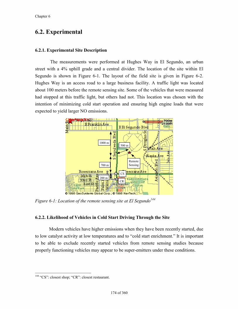
Chapter 6

174 of 360

6.2. Experimental

6.2.1. Experimental Site Description

The measurements were performed at Hughes Way in El Segundo, an urban

street with a 4% uphill grade and a central divider. The location of the site within El

Segundo is shown in Figure 6-1. The layout of the field site is given in Figure 6-2.

Hughes Way is an access road to a large business facility. A traffic light was located

about 100 meters before the remote sensing site. Some of the vehicles that were measured

had stopped at this traffic light, but others had not. This location was chosen with the

intention of minimizing cold start operation and ensuring high engine loads that were

expected to yield larger NO emissions.

RemoteSensing700 m

1000 m500 m

CR

CS200 m

Figure 6-1: Location of the remote sensing site at El Segundo144

6.2.2. Likelihood of Vehicles in Cold Start Driving Through the Site

Modern vehicles have higher emissions when they have been recently started, due

to low catalyst activity at low temperatures and to “cold start enrichment.” It is important

to be able to exclude recently started vehicles from remote sensing studies because

properly functioning vehicles may appear to be super-emitters under these conditions.

144 “CS”: closest shop; “CR”: closest restaurant.

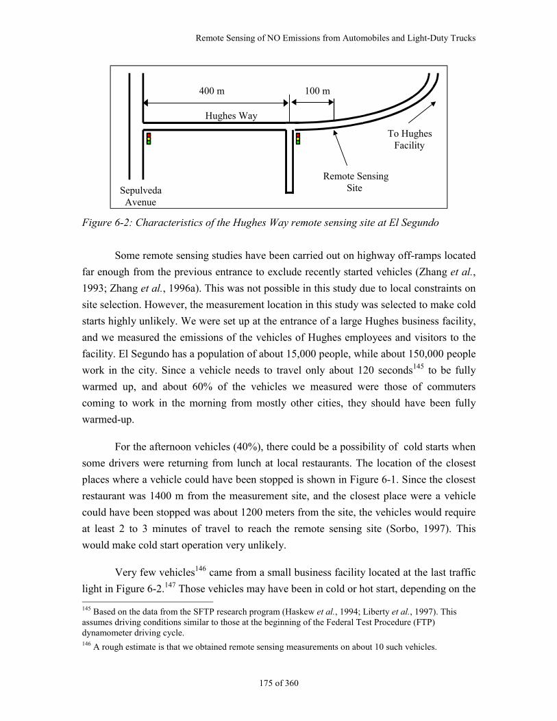
Remote Sensing of NO Emissions from Automobiles and Light-Duty Trucks

175 of 360

SepulvedaAvenue

Hughes Way

Remote SensingSite

400 m 100 m

To HughesFacility

Figure 6-2: Characteristics of the Hughes Way remote sensing site at El Segundo

Some remote sensing studies have been carried out on highway off-ramps located

far enough from the previous entrance to exclude recently started vehicles (Zhang et al.,

1993; Zhang et al., 1996a). This was not possible in this study due to local constraints on

site selection. However, the measurement location in this study was selected to make cold

starts highly unlikely. We were set up at the entrance of a large Hughes business facility,

and we measured the emissions of the vehicles of Hughes employees and visitors to the

facility. El Segundo has a population of about 15,000 people, while about 150,000 people

work in the city. Since a vehicle needs to travel only about 120 seconds145 to be fully

warmed up, and about 60% of the vehicles we measured were those of commuters

coming to work in the morning from mostly other cities, they should have been fully

warmed-up.

For the afternoon vehicles (40%), there could be a possibility of cold starts when

some drivers were returning from lunch at local restaurants. The location of the closest

places where a vehicle could have been stopped is shown in Figure 6-1. Since the closest

restaurant was 1400 m from the measurement site, and the closest place were a vehicle

could have been stopped was about 1200 meters from the site, the vehicles would require

at least 2 to 3 minutes of travel to reach the remote sensing site (Sorbo, 1997). This

would make cold start operation very unlikely.

Very few vehicles146 came from a small business facility located at the last traffic

light in Figure 6-2.147 Those vehicles may have been in cold or hot start, depending on the 145 Based on the data from the SFTP research program (Haskew et al., 1994; Liberty et al., 1997). Thisassumes driving conditions similar to those at the beginning of the Federal Test Procedure (FTP)dynamometer driving cycle.146 A rough estimate is that we obtained remote sensing measurements on about 10 such vehicles.

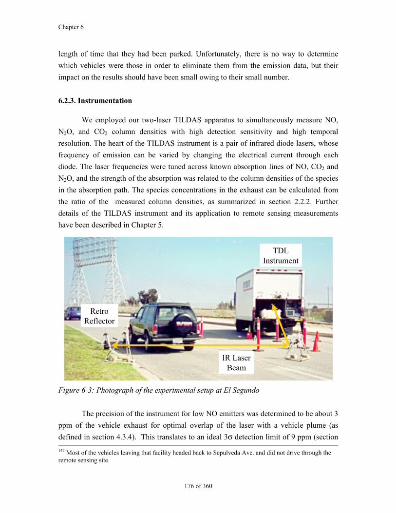
Chapter 6

176 of 360

length of time that they had been parked. Unfortunately, there is no way to determine

which vehicles were those in order to eliminate them from the emission data, but their

impact on the results should have been small owing to their small number.

6.2.3. Instrumentation

We employed our two-laser TILDAS apparatus to simultaneously measure NO,

N2O, and CO2 column densities with high detection sensitivity and high temporal

resolution. The heart of the TILDAS instrument is a pair of infrared diode lasers, whose

frequency of emission can be varied by changing the electrical current through each

diode. The laser frequencies were tuned across known absorption lines of NO, CO2 and

N2O, and the strength of the absorption was related to the column densities of the species

in the absorption path. The species concentrations in the exhaust can be calculated from

the ratio of the measured column densities, as summarized in section 2.2.2. Further

details of the TILDAS instrument and its application to remote sensing measurements

have been described in Chapter 5.

RetroReflector

TDLInstrument

IR LaserBeam

Figure 6-3: Photograph of the experimental setup at El Segundo

The precision of the instrument for low NO emitters was determined to be about 3

ppm of the vehicle exhaust for optimal overlap of the laser with a vehicle plume (as

defined in section 4.3.4). This translates to an ideal 3σ detection limit of 9 ppm (section 147 Most of the vehicles leaving that facility headed back to Sepulveda Ave. and did not drive through theremote sensing site.

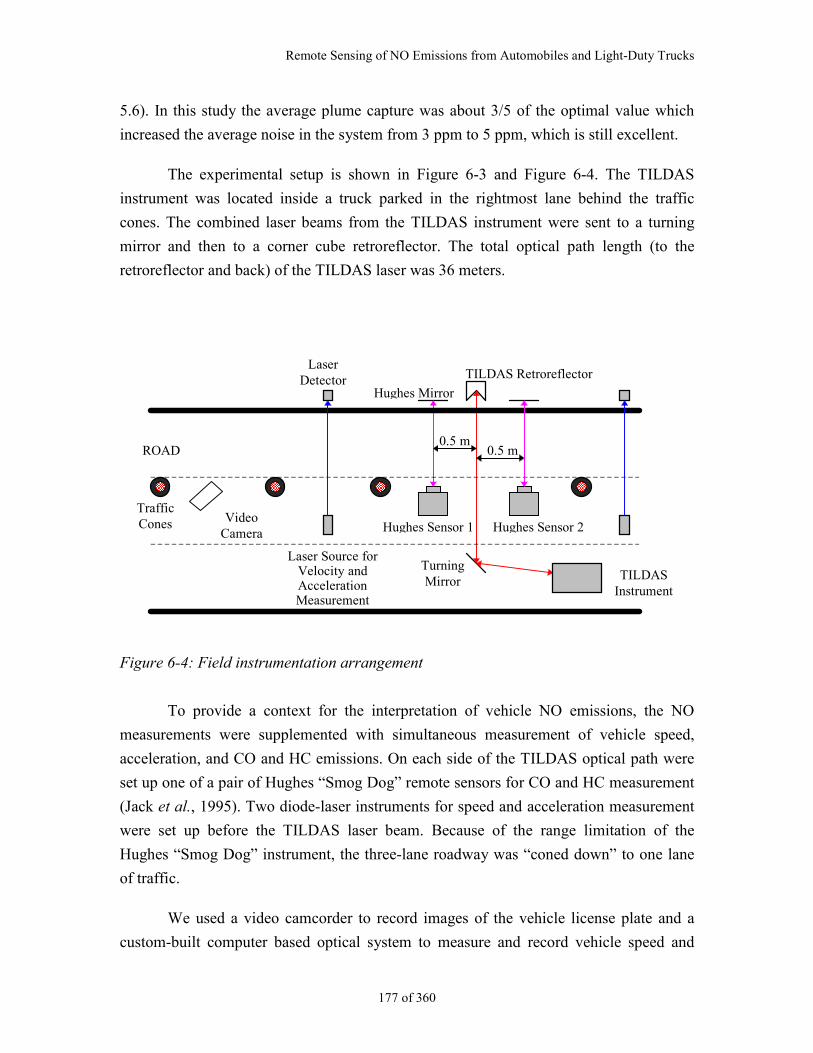
Remote Sensing of NO Emissions from Automobiles and Light-Duty Trucks

177 of 360

5.6). In this study the average plume capture was about 3/5 of the optimal value which

increased the average noise in the system from 3 ppm to 5 ppm, which is still excellent.

The experimental setup is shown in Figure 6-3 and Figure 6-4. The TILDAS

instrument was located inside a truck parked in the rightmost lane behind the traffic

cones. The combined laser beams from the TILDAS instrument were sent to a turning

mirror and then to a corner cube retroreflector. The total optical path length (to the

retroreflector and back) of the TILDAS laser was 36 meters.

Hughes Mirror

TILDAS Retroreflector

Hughes Sensor 1

TILDASInstrument

Hughes Sensor 2

0.5 m0.5 mROAD

TrafficCones

TurningMirror

VideoCamera

Laser Source forVelocity andAccelerationMeasurement

LaserDetector

������������

����������

��������������

������������

Figure 6-4: Field instrumentation arrangement

To provide a context for the interpretation of vehicle NO emissions, the NO

measurements were supplemented with simultaneous measurement of vehicle speed,

acceleration, and CO and HC emissions. On each side of the TILDAS optical path were

set up one of a pair of Hughes “Smog Dog” remote sensors for CO and HC measurement

(Jack et al., 1995). Two diode-laser instruments for speed and acceleration measurement

were set up before the TILDAS laser beam. Because of the range limitation of the

Hughes “Smog Dog” instrument, the three-lane roadway was “coned down” to one lane

of traffic.

We used a video camcorder to record images of the vehicle license plate and a

custom-built computer based optical system to measure and record vehicle speed and

Chapter 6

178 of 360

acceleration data. Vehicle make, model year and identification number (VIN) were

retrieved from the California Department of Motor Vehicles (DMV) from the recorded

license plate data.

6.2.4. Vehicle Speed and Acceleration Measurement

A low-cost, laser diode-based instrument was developed by EMDOT Corporation

to provide an accurate means of measuring vehicle speed and acceleration that would be

compatible with the remote sensing field environment. This instrument timed with

microsecond accuracy the interruption of two light beams directed perpendicularly across

the vehicle path from two roadside sources onto two photo detectors on the opposite side

of the road. The two stations were separated by about 10 meters. The two station setup

provided the necessary information needed to calculate the speed and a constant rate of

acceleration for the vehicle between the two stations.

The precision of the speed and acceleration data are estimated148 to be 0.033 m/s

(0.07 mph) and 0.05 m/s2 (0.11 mph/s), respectively. This represents a fractional accuracy

of 0.2% of the range of velocities and of 1.3% of the range of accelerations observed in

this study.

The average speed of the vehicles with valid NO emission measurements was

13.9 m/s ± 2.6 m/s (31.1 ± 5.8 mph). The average acceleration was 0.59 m/s2 ± 0.49 m/s2

(1.32 ± 1.10 mph/s). This includes the effect of roadway grade since the forces due to

acceleration and grade are indistinguishable. Two-thirds of the average acceleration was

due to the 4% road grade, which contributes 0.4 m/s2.

6.2.5. License Plate Data Acquisition

The last component of the remote sensing data acquisition system was the license

plate imaging equipment. In order to obtain vehicle information such as model year,

make, vehicle identification number (VIN), etc. from a source such as the California

Department of Motor Vehicles (DMV), it was necessary to obtain a readable image of

each vehicle’s license plate as it passed through the emissions measurement station. In

addition, each license plate image required a time stamp that was synchronized with the

TILDAS instrument clock. This was necessary so that the corresponding license plate 148 The precision of these measurements was estimated from the calculated length of those vehicles thatwere measured more than once.

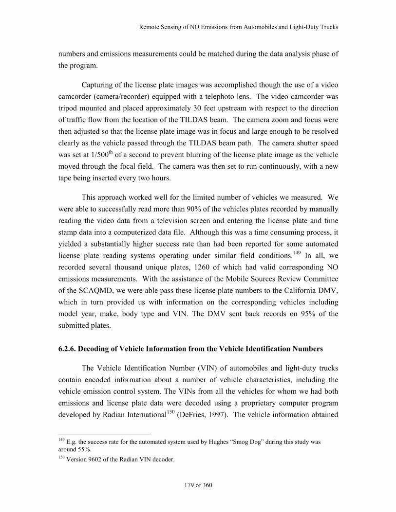
Remote Sensing of NO Emissions from Automobiles and Light-Duty Trucks

179 of 360

numbers and emissions measurements could be matched during the data analysis phase of

the program.

Capturing of the license plate images was accomplished though the use of a video

camcorder (camera/recorder) equipped with a telephoto lens. The video camcorder was

tripod mounted and placed approximately 30 feet upstream with respect to the direction

of traffic flow from the location of the TILDAS beam. The camera zoom and focus were

then adjusted so that the license plate image was in focus and large enough to be resolved

clearly as the vehicle passed through the TILDAS beam path. The camera shutter speed

was set at 1/500th of a second to prevent blurring of the license plate image as the vehicle

moved through the focal field. The camera was then set to run continuously, with a new

tape being inserted every two hours.

This approach worked well for the limited number of vehicles we measured. We

were able to successfully read more than 90% of the vehicles plates recorded by manually

reading the video data from a television screen and entering the license plate and time

stamp data into a computerized data file. Although this was a time consuming process, it

yielded a substantially higher success rate than had been reported for some automated

license plate reading systems operating under similar field conditions.149 In all, we

recorded several thousand unique plates, 1260 of which had valid corresponding NO

emissions measurements. With the assistance of the Mobile Sources Review Committee

of the SCAQMD, we were able pass these license plate numbers to the California DMV,

which in turn provided us with information on the corresponding vehicles including

model year, make, body type and VIN. The DMV sent back records on 95% of the

submitted plates.

6.2.6. Decoding of Vehicle Information from the Vehicle Identification Numbers

The Vehicle Identification Number (VIN) of automobiles and light-duty trucks

contain encoded information about a number of vehicle characteristics, including the

vehicle emission control system. The VINs from all the vehicles for whom we had both

emissions and license plate data were decoded using a proprietary computer program

developed by Radian International150 (DeFries, 1997). The vehicle information obtained

149 E.g. the success rate for the automated system used by Hughes “Smog Dog” during this study wasaround 55%.150 Version 9602 of the Radian VIN decoder.

Chapter 6

180 of 360

by decoding the VINs is summarized in Table 6-1. About 10% of the VINs supplied by

the California DMV contained errors and could not be decoded.

FIELD Meaning

YEAR Model YearMAKE Vehicle MakeSERIES Vehicle ModelBODY Body StyleDISP Engine DisplacementUN Units for Displacement (cubic inches/liters)

CYL Cylinder ConfigurationASP Aspiration (Normal/Turbocharged/Supercharged)IND Fuel Induction (Carburetted/Fuel Injected/Diesel/CNG/LPG)AIR Air Injection ReactorEVP Evaporative Emissions ControlsOXY Oxidation (Two-way) CatalystTWC Three Way CatalystEGR Exhaust Gas RecirculationCLL Closed Loop Combustion ControlPCV Positive Crankcase VentilationTAC Thermostatic Air Cleaner

MANUFACTURERCNTRY Country of ManufactureTYPE Vehicle Type (CAR/MPV/TRK/Other)

GVWR Gross Vehicle Weight Rating (pounds)

Table 6-1: Summary of the output parameters provided by the Radian VIN decoder forevery vehicle

Some of this information was already available to us from the DMV records

(model year, make, manufacturer, and some information on body type), but most of it

was not.

The TYPE field permitted to distinguish between vehicles subject to the

passenger car and the light duty truck emission standards (DeFries, 1997; Good, 1998).

Only vehicles classified as “CAR” were subject to the passenger car standards, while

vehicles classified as “TRK,” “MPV” (multi-purpose vehicle), “VAN,” and “BUS” were

subject to the light-duty truck standards. Vehicles classified as “INC” (incomplete) could

be subject to either standards.

Remote Sensing of NO Emissions from Automobiles and Light-Duty Trucks

181 of 360

6.2.7. CO and HC Remote Sensing

As mentioned above, during our two days of measurements at El Segundo a pair

of non-dispersive infrared (NDIR) “Smog Dog” remote sensors from Hughes SBRC

(Jack et al., 1995) were used to measure CO and HC emissions simultaneously with our

NO emission measurement. The two Hughes instruments were located 0.5 meters before

and after the TILDAS laser path, as indicated in Figure 6-4.

The detection limits for this system were 200 ppm for CO and 30 ppm for HC

(Jack et al., 1995). These systems also included and NO emission channel by a non-

dispersive infrared method with a stated detection limit of 500 ppm of the exhaust (Jack

et al., 1995). NO data were acquired but Hughes did not authorize us to present the

results.

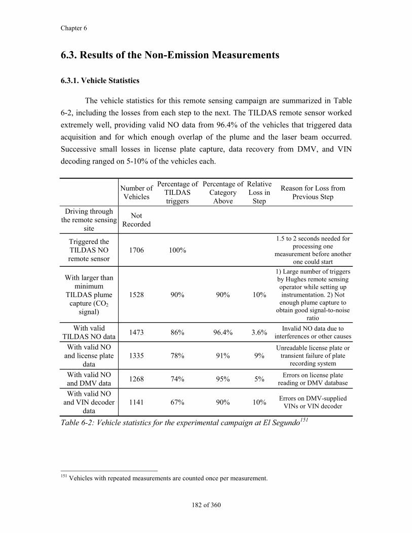
Chapter 6

182 of 360

6.3. Results of the Non-Emission Measurements

6.3.1. Vehicle Statistics

The vehicle statistics for this remote sensing campaign are summarized in Table

6-2, including the losses from each step to the next. The TILDAS remote sensor worked

extremely well, providing valid NO data from 96.4% of the vehicles that triggered data

acquisition and for which enough overlap of the plume and the laser beam occurred.

Successive small losses in license plate capture, data recovery from DMV, and VIN

decoding ranged on 5-10% of the vehicles each.

Number ofVehicles

Percentage ofTILDAStriggers

Percentage ofCategoryAbove

RelativeLoss in

Step

Reason for Loss fromPrevious Step

Driving throughthe remote sensing

site

NotRecorded

Triggered theTILDAS NOremote sensor

1706 100%

1.5 to 2 seconds needed forprocessing one

measurement before anotherone could start

With larger thanminimum

TILDAS plumecapture (CO2

signal)

1528 90% 90% 10%

1) Large number of triggersby Hughes remote sensingoperator while setting upinstrumentation. 2) Not

enough plume capture toobtain good signal-to-noise

ratio

With validTILDAS NO data

1473 86% 96.4% 3.6%Invalid NO data due to

interferences or other causes

With valid NOand license plate

data1335 78% 91% 9%

Unreadable license plate ortransient failure of plate

recording system

With valid NOand DMV data

1268 74% 95% 5%Errors on license plate

reading or DMV database

With valid NOand VIN decoder

data1141 67% 90% 10%

Errors on DMV-suppliedVINs or VIN decoder

Table 6-2: Vehicle statistics for the experimental campaign at El Segundo151

151 Vehicles with repeated measurements are counted once per measurement.

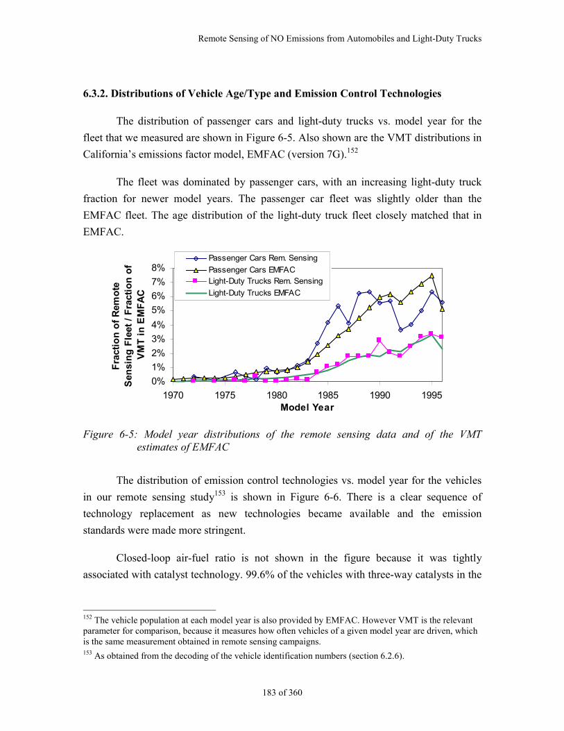
Remote Sensing of NO Emissions from Automobiles and Light-Duty Trucks

183 of 360

6.3.2. Distributions of Vehicle Age/Type and Emission Control Technologies

The distribution of passenger cars and light-duty trucks vs. model year for the

fleet that we measured are shown in Figure 6-5. Also shown are the VMT distributions in

California’s emissions factor model, EMFAC (version 7G).152

The fleet was dominated by passenger cars, with an increasing light-duty truck

fraction for newer model years. The passenger car fleet was slightly older than the

EMFAC fleet. The age distribution of the light-duty truck fleet closely matched that in

EMFAC.

0%

1%

2%

3%

4%

5%

6%

7%

8%

1970 1975 1980 1985 1990 1995Model Year

Fra

ctio

n o

f R

emo

te

Sen

sin

g F

leet

/ F

ract

ion

of

VM

T i

n E

MF

AC

Passenger Cars Rem. Sensing

Passenger Cars EMFACLight-Duty Trucks Rem. Sensing

Light-Duty Trucks EMFAC

Figure 6-5: Model year distributions of the remote sensing data and of the VMTestimates of EMFAC

The distribution of emission control technologies vs. model year for the vehicles

in our remote sensing study153 is shown in Figure 6-6. There is a clear sequence of

technology replacement as new technologies became available and the emission

standards were made more stringent.

Closed-loop air-fuel ratio is not shown in the figure because it was tightly

associated with catalyst technology. 99.6% of the vehicles with three-way catalysts in the

152 The vehicle population at each model year is also provided by EMFAC. However VMT is the relevantparameter for comparison, because it measures how often vehicles of a given model year are driven, whichis the same measurement obtained in remote sensing campaigns.153 As obtained from the decoding of the vehicle identification numbers (section 6.2.6).

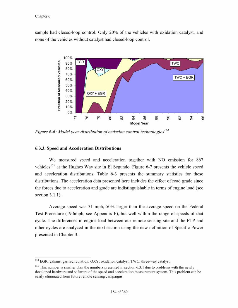
Chapter 6

184 of 360

sample had closed-loop control. Only 20% of the vehicles with oxidation catalyst, and

none of the vehicles without catalyst had closed-loop control.

0%

10%

20%

30%

40%

50%

60%

70%

80%

90%

100%

71

76

78

80

82

84

86

88

90

92

94

96

Model Year

Fra

cti

on

of

Me

as

ure

d V

eh

icle

s EGR

OXY + EGR

TWC + EGR

TWC

OXY

Figure 6-6: Model year distribution of emission control technologies154

6.3.3. Speed and Acceleration Distributions

We measured speed and acceleration together with NO emission for 867

vehicles155 at the Hughes Way site in El Segundo. Figure 6-7 presents the vehicle speed

and acceleration distributions. Table 6-3 presents the summary statistics for these

distributions. The acceleration data presented here includes the effect of road grade since

the forces due to acceleration and grade are indistinguishable in terms of engine load (see

section 3.1.1).

Average speed was 31 mph, 50% larger than the average speed on the Federal

Test Procedure (19.6mph, see Appendix F), but well within the range of speeds of that

cycle. The differences in engine load between our remote sensing site and the FTP and

other cycles are analyzed in the next section using the new definition of Specific Power

presented in Chapter 3.

154 EGR: exhaust gas recirculation; OXY: oxidation catalyst; TWC: three-way catalyst.155 This number is smaller than the numbers presented in section 6.3.1 due to problems with the newlydeveloped hardware and software of the speed and acceleration measurement system. This problem can beeasily eliminated from future remote sensing campaigns.

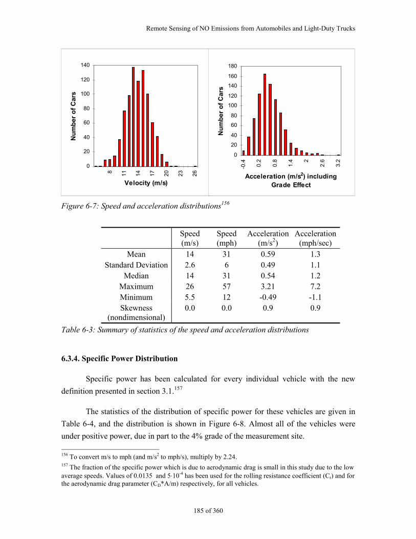
Remote Sensing of NO Emissions from Automobiles and Light-Duty Trucks

185 of 360

0

20

40

60

80

100

120

140

8 11

14

17

20

23

26

Velocity (m/s)

Nu

mb

er o

f C

ars

0

20

40

60

80

100

120

140

160

180

-0.4 0.2

0.8

1.4 2

2.6

3.2

Acceleration (m/s2) including Grade Effect

Nu

mb

er o

f C

ars

Figure 6-7: Speed and acceleration distributions156

Speed(m/s)

Speed(mph)

Acceleration(m/s2)

Acceleration(mph/sec)

Mean 14 31 0.59 1.3Standard Deviation 2.6 6 0.49 1.1

Median 14 31 0.54 1.2Maximum 26 57 3.21 7.2Minimum 5.5 12 -0.49 -1.1Skewness

(nondimensional)0.0 0.0 0.9 0.9

Table 6-3: Summary of statistics of the speed and acceleration distributions

6.3.4. Specific Power Distribution

Specific power has been calculated for every individual vehicle with the new

definition presented in section 3.1.157

The statistics of the distribution of specific power for these vehicles are given in

Table 6-4, and the distribution is shown in Figure 6-8. Almost all of the vehicles were

under positive power, due in part to the 4% grade of the measurement site.

156 To convert m/s to mph (and m/s2 to mph/s), multiply by 2.24.157 The fraction of the specific power which is due to aerodynamic drag is small in this study due to the lowaverage speeds. Values of 0.0135 and 5⋅10-4 has been used for the rolling resistance coefficient (Cr) and forthe aerodynamic drag parameter (CD*A/m) respectively, for all vehicles.

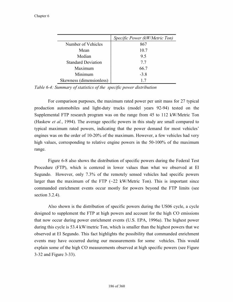
Chapter 6

186 of 360

Specific Power (kW/Metric Ton)

Number of Vehicles 867Mean 10.7

Median 9.5Standard Deviation 7.7

Maximum 66.7Minimum -3.8

Skewness (dimensionless) 1.7

Table 6-4: Summary of statistics of the specific power distribution

For comparison purposes, the maximum rated power per unit mass for 27 typical

production automobiles and light-duty trucks (model years 92-94) tested on the

Supplemental FTP research program was on the range from 45 to 112 kW/Metric Ton

(Haskew et al., 1994). The average specific powers in this study are small compared to

typical maximum rated powers, indicating that the power demand for most vehicles’

engines was on the order of 10-20% of the maximum. However, a few vehicles had very

high values, corresponding to relative engine powers in the 50-100% of the maximum

range.

Figure 6-8 also shows the distribution of specific powers during the Federal Test

Procedure (FTP), which is centered in lower values than what we observed at El

Segundo. However, only 7.3% of the remotely sensed vehicles had specific powers

larger than the maximum of the FTP (~22 kW/Metric Ton). This is important since

commanded enrichment events occur mostly for powers beyond the FTP limits (see

section 3.2.4).

Also shown is the distribution of specific powers during the US06 cycle, a cycle

designed to supplement the FTP at high powers and account for the high CO emissions

that now occur during power enrichment events (U.S. EPA, 1996a). The highest power

during this cycle is 53.4 kW/metric Ton, which is smaller than the highest powers that we

observed at El Segundo. This fact highlights the possibility that commanded enrichment

events may have occurred during our measurements for some vehicles. This would

explain some of the high CO measurements observed at high specific powers (see Figure

3-32 and Figure 3-33).

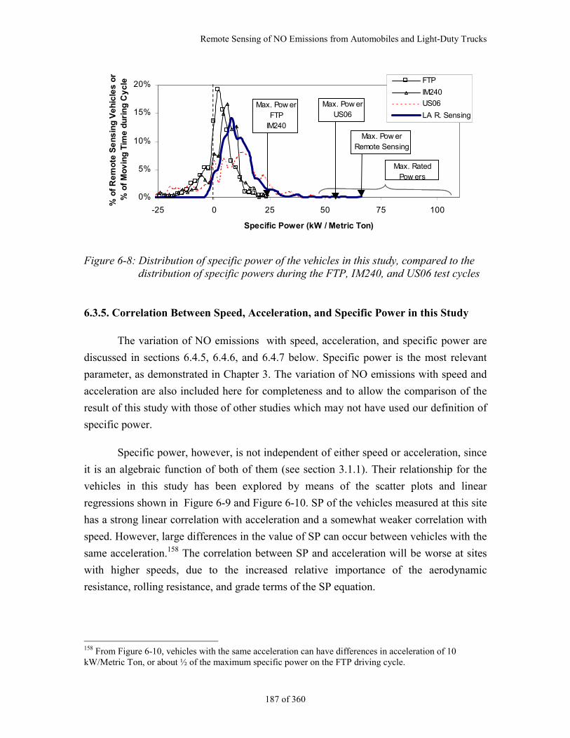
Remote Sensing of NO Emissions from Automobiles and Light-Duty Trucks

187 of 360

0%

5%

10%

15%

20%

-25 0 25 50 75 100

Specific Power (kW / Metric Ton)

% o

f R

em

ote

Se

ns

ing

Ve

hic

les

or

% o

f M

ov

ing

Tim

e d

uri

ng

Cy

cle FTP

IM240

US06

LA R. SensingMax. Pow er

FTPIM240

Max. Rated Pow ers

Max. Pow erRemote Sensing

Max. Pow erUS06

Figure 6-8: Distribution of specific power of the vehicles in this study, compared to thedistribution of specific powers during the FTP, IM240, and US06 test cycles

6.3.5. Correlation Between Speed, Acceleration, and Specific Power in this Study

The variation of NO emissions with speed, acceleration, and specific power are

discussed in sections 6.4.5, 6.4.6, and 6.4.7 below. Specific power is the most relevant

parameter, as demonstrated in Chapter 3. The variation of NO emissions with speed and

acceleration are also included here for completeness and to allow the comparison of the

result of this study with those of other studies which may not have used our definition of

specific power.

Specific power, however, is not independent of either speed or acceleration, since

it is an algebraic function of both of them (see section 3.1.1). Their relationship for the

vehicles in this study has been explored by means of the scatter plots and linear

regressions shown in Figure 6-9 and Figure 6-10. SP of the vehicles measured at this site

has a strong linear correlation with acceleration and a somewhat weaker correlation with

speed. However, large differences in the value of SP can occur between vehicles with the

same acceleration.158 The correlation between SP and acceleration will be worse at sites

with higher speeds, due to the increased relative importance of the aerodynamic

resistance, rolling resistance, and grade terms of the SP equation.

158 From Figure 6-10, vehicles with the same acceleration can have differences in acceleration of 10kW/Metric Ton, or about ½ of the maximum specific power on the FTP driving cycle.

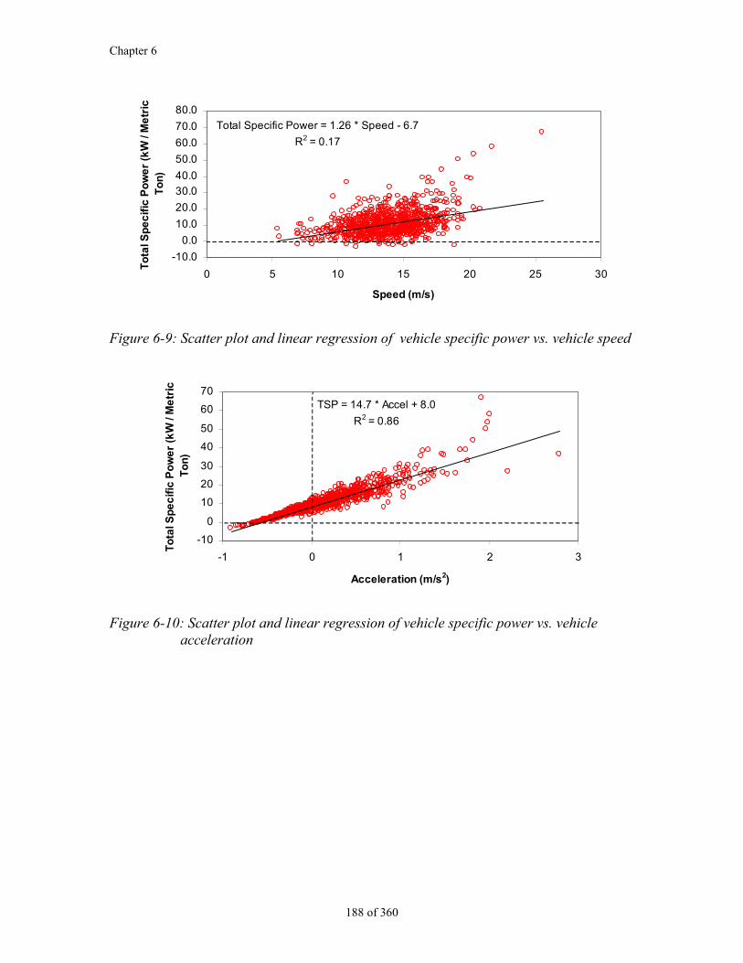
Chapter 6

188 of 360

Total Specific Power = 1.26 * Speed - 6.7

R2 = 0.17

-10.0

0.0

10.0

20.0

30.0

40.0

50.0

60.0

70.0

80.0

0 5 10 15 20 25 30

Speed (m/s)

To

tal S

pe

cif

ic P

ow

er

(kW

/ M

etr

ic

To

n)

Figure 6-9: Scatter plot and linear regression of vehicle specific power vs. vehicle speed

TSP = 14.7 * Accel + 8.0

R2 = 0.86

-10

0

10

20

30

40

50

60

70

-1 0 1 2 3

Acceleration (m/s2)

To

tal S

pe

cif

ic P

ow

er

(kW

/ M

etr

ic

To

n)

Figure 6-10: Scatter plot and linear regression of vehicle specific power vs. vehicleacceleration

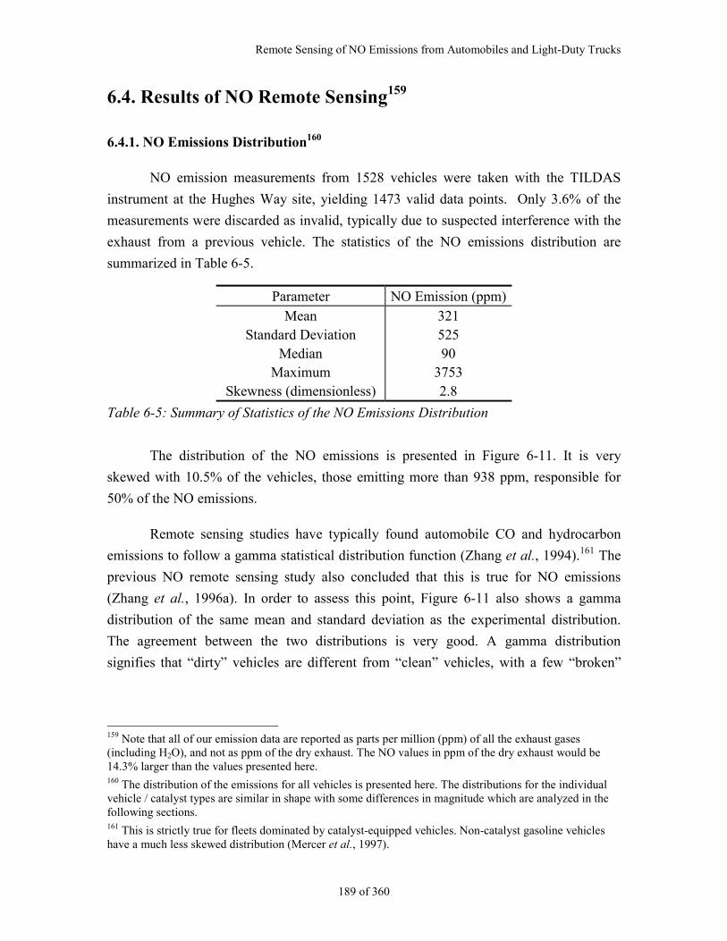
Remote Sensing of NO Emissions from Automobiles and Light-Duty Trucks

189 of 360

6.4. Results of NO Remote Sensing159

6.4.1. NO Emissions Distribution160

NO emission measurements from 1528 vehicles were taken with the TILDAS

instrument at the Hughes Way site, yielding 1473 valid data points. Only 3.6% of the

measurements were discarded as invalid, typically due to suspected interference with the

exhaust from a previous vehicle. The statistics of the NO emissions distribution are

summarized in Table 6-5.

Parameter NO Emission (ppm)

Mean 321Standard Deviation 525

Median 90Maximum 3753

Skewness (dimensionless) 2.8

Table 6-5: Summary of Statistics of the NO Emissions Distribution

The distribution of the NO emissions is presented in Figure 6-11. It is very

skewed with 10.5% of the vehicles, those emitting more than 938 ppm, responsible for

50% of the NO emissions.

Remote sensing studies have typically found automobile CO and hydrocarbon

emissions to follow a gamma statistical distribution function (Zhang et al., 1994).161 The

previous NO remote sensing study also concluded that this is true for NO emissions

(Zhang et al., 1996a). In order to assess this point, Figure 6-11 also shows a gamma

distribution of the same mean and standard deviation as the experimental distribution.

The agreement between the two distributions is very good. A gamma distribution

signifies that “dirty” vehicles are different from “clean” vehicles, with a few “broken”

159 Note that all of our emission data are reported as parts per million (ppm) of all the exhaust gases(including H2O), and not as ppm of the dry exhaust. The NO values in ppm of the dry exhaust would be14.3% larger than the values presented here.160 The distribution of the emissions for all vehicles is presented here. The distributions for the individualvehicle / catalyst types are similar in shape with some differences in magnitude which are analyzed in thefollowing sections.161 This is strictly true for fleets dominated by catalyst-equipped vehicles. Non-catalyst gasoline vehicleshave a much less skewed distribution (Mercer et al., 1997).

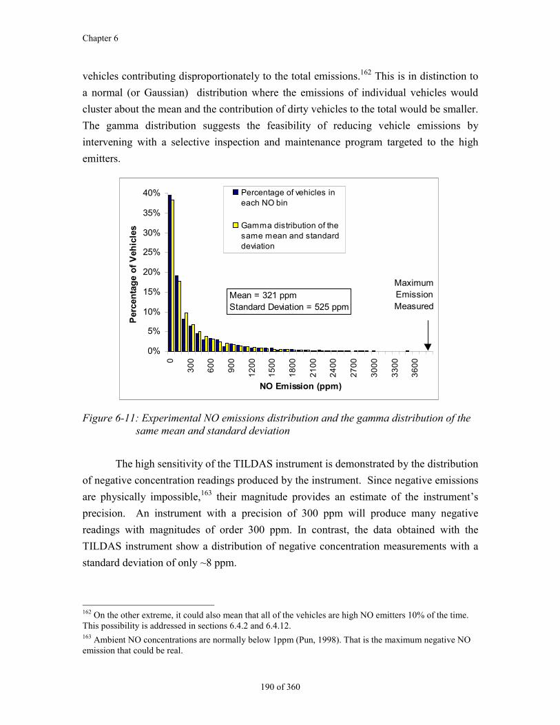
Chapter 6

190 of 360

vehicles contributing disproportionately to the total emissions.162 This is in distinction to

a normal (or Gaussian) distribution where the emissions of individual vehicles would

cluster about the mean and the contribution of dirty vehicles to the total would be smaller.

The gamma distribution suggests the feasibility of reducing vehicle emissions by

intervening with a selective inspection and maintenance program targeted to the high

emitters.

0%

5%

10%

15%

20%

25%

30%

35%

40%

0

30

0

60

0

90

0

12

00

15

00

18

00

21

00

24

00

27

00

30

00

33

00

36

00

NO Emission (ppm)

Per

cen

tag

e o

f V

ehic

les

Percentage of vehicles ineach NO bin

Gamma distribution of thesame mean and standarddeviation

Mean = 321 ppmStandard Deviation = 525 ppm

Maximum Emission Measured

Figure 6-11: Experimental NO emissions distribution and the gamma distribution of thesame mean and standard deviation

The high sensitivity of the TILDAS instrument is demonstrated by the distribution

of negative concentration readings produced by the instrument. Since negative emissions

are physically impossible,163 their magnitude provides an estimate of the instrument’s

precision. An instrument with a precision of 300 ppm will produce many negative

readings with magnitudes of order 300 ppm. In contrast, the data obtained with the

TILDAS instrument show a distribution of negative concentration measurements with a

standard deviation of only ~8 ppm.

162 On the other extreme, it could also mean that all of the vehicles are high NO emitters 10% of the time.This possibility is addressed in sections 6.4.2 and 6.4.12.163 Ambient NO concentrations are normally below 1ppm (Pun, 1998). That is the maximum negative NOemission that could be real.

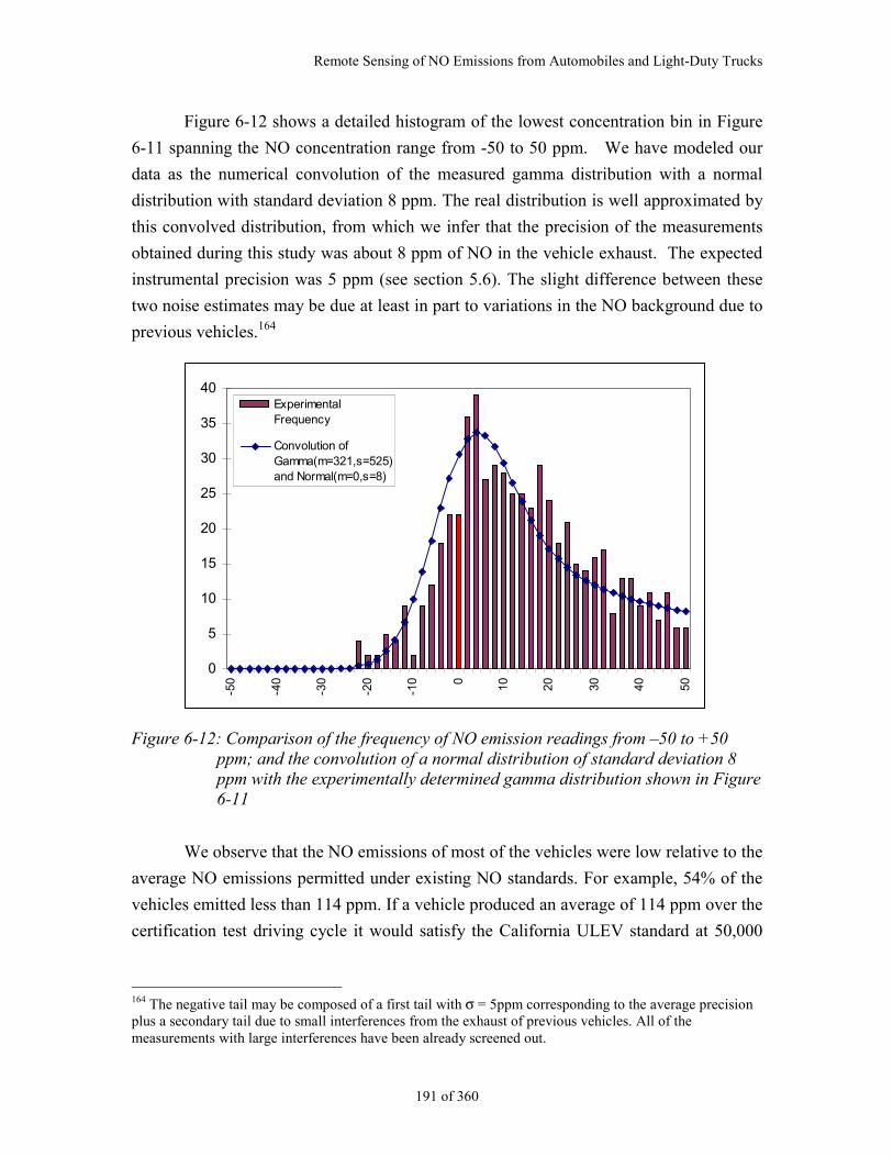
Remote Sensing of NO Emissions from Automobiles and Light-Duty Trucks

191 of 360

Figure 6-12 shows a detailed histogram of the lowest concentration bin in Figure

6-11 spanning the NO concentration range from -50 to 50 ppm. We have modeled our

data as the numerical convolution of the measured gamma distribution with a normal

distribution with standard deviation 8 ppm. The real distribution is well approximated by

this convolved distribution, from which we infer that the precision of the measurements

obtained during this study was about 8 ppm of NO in the vehicle exhaust. The expected

instrumental precision was 5 ppm (see section 5.6). The slight difference between these

two noise estimates may be due at least in part to variations in the NO background due to

previous vehicles.164

0

5

10

15

20

25

30

35

40

-50

-40

-30

-20

-10 0 10 20 30 40 50

ExperimentalFrequency

Convolution ofGamma(m=321,s=525)and Normal(m=0,s=8)

Figure 6-12: Comparison of the frequency of NO emission readings from –50 to +50ppm; and the convolution of a normal distribution of standard deviation 8ppm with the experimentally determined gamma distribution shown in Figure6-11

We observe that the NO emissions of most of the vehicles were low relative to the

average NO emissions permitted under existing NO standards. For example, 54% of the

vehicles emitted less than 114 ppm. If a vehicle produced an average of 114 ppm over the

certification test driving cycle it would satisfy the California ULEV standard at 50,000

164 The negative tail may be composed of a first tail with σ = 5ppm corresponding to the average precisionplus a secondary tail due to small interferences from the exhaust of previous vehicles. All of themeasurements with large interferences have been already screened out.

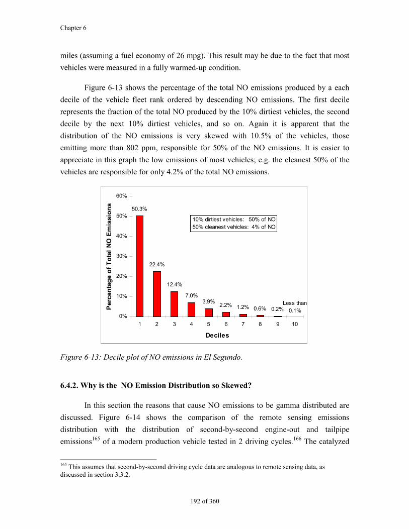
Chapter 6

192 of 360

miles (assuming a fuel economy of 26 mpg). This result may be due to the fact that most

vehicles were measured in a fully warmed-up condition.

Figure 6-13 shows the percentage of the total NO emissions produced by a each

decile of the vehicle fleet rank ordered by descending NO emissions. The first decile

represents the fraction of the total NO produced by the 10% dirtiest vehicles, the second

decile by the next 10% dirtiest vehicles, and so on. Again it is apparent that the

distribution of the NO emissions is very skewed with 10.5% of the vehicles, those

emitting more than 802 ppm, responsible for 50% of the NO emissions. It is easier to

appreciate in this graph the low emissions of most vehicles; e.g. the cleanest 50% of the

vehicles are responsible for only 4.2% of the total NO emissions.

50.3%

22.4%

12.4%

7.0%3.9%

2.2% 1.2% 0.6% 0.2%Less than

0.1%0%

10%

20%

30%

40%

50%

60%

1 2 3 4 5 6 7 8 9 10

Deciles

Per

cen

tag

e o

f T

ota

l N

O E

mis

sio

ns

10% dirtiest vehicles: 50% of NO50% cleanest vehicles: 4% of NO

Figure 6-13: Decile plot of NO emissions in El Segundo.

6.4.2. Why is the NO Emission Distribution so Skewed?

In this section the reasons that cause NO emissions to be gamma distributed are

discussed. Figure 6-14 shows the comparison of the remote sensing emissions

distribution with the distribution of second-by-second engine-out and tailpipe

emissions165 of a modern production vehicle tested in 2 driving cycles.166 The catalyzed

165 This assumes that second-by-second driving cycle data are analogous to remote sensing data, asdiscussed in section 3.3.2.

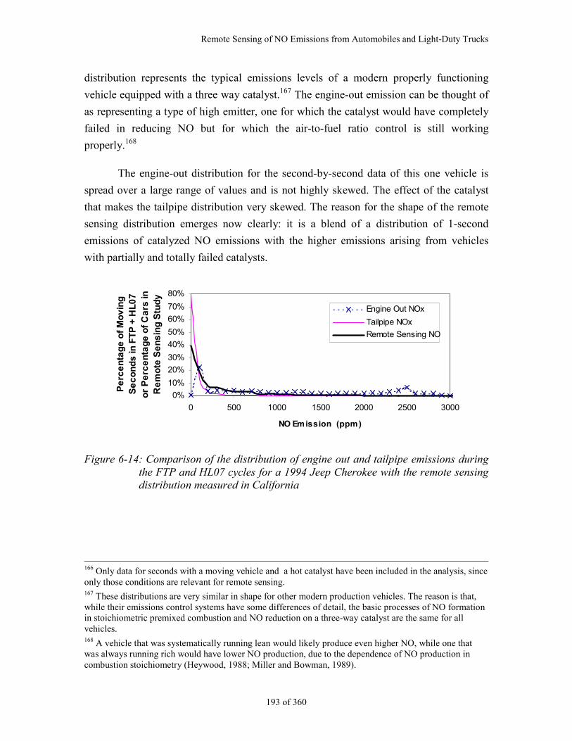
Remote Sensing of NO Emissions from Automobiles and Light-Duty Trucks

193 of 360

distribution represents the typical emissions levels of a modern properly functioning

vehicle equipped with a three way catalyst.167 The engine-out emission can be thought of

as representing a type of high emitter, one for which the catalyst would have completely

failed in reducing NO but for which the air-to-fuel ratio control is still working

properly.168

The engine-out distribution for the second-by-second data of this one vehicle is

spread over a large range of values and is not highly skewed. The effect of the catalyst

that makes the tailpipe distribution very skewed. The reason for the shape of the remote

sensing distribution emerges now clearly: it is a blend of a distribution of 1-second

emissions of catalyzed NO emissions with the higher emissions arising from vehicles

with partially and totally failed catalysts.

0%

10%

20%

30%

40%

50%

60%

70%

80%

0 500 1000 1500 2000 2500 3000

NO Emission (ppm)

Pe

rce

nta

ge

of

Mo

vin

g

Se

co

nd

s in

FT

P +

HL

07

or

Pe

rce

nta

ge

of

Ca

rs in

R

em

ote

Se

ns

ing

Stu

dy

Engine Out NOx

Tailpipe NOx

Remote Sensing NO

Figure 6-14: Comparison of the distribution of engine out and tailpipe emissions duringthe FTP and HL07 cycles for a 1994 Jeep Cherokee with the remote sensingdistribution measured in California

166 Only data for seconds with a moving vehicle and a hot catalyst have been included in the analysis, sinceonly those conditions are relevant for remote sensing.167 These distributions are very similar in shape for other modern production vehicles. The reason is that,while their emissions control systems have some differences of detail, the basic processes of NO formationin stoichiometric premixed combustion and NO reduction on a three-way catalyst are the same for allvehicles.168 A vehicle that was systematically running lean would likely produce even higher NO, while one thatwas always running rich would have lower NO production, due to the dependence of NO production incombustion stoichiometry (Heywood, 1988; Miller and Bowman, 1989).

Chapter 6

194 of 360

6.4.3. Comparison to NOx Emission Factors and Ratios from Other Studies

The emission factor for this study has been estimated at 8.1 ± 0.13 grams of NO

per kg of gasoline169, 170, 171 based on the results presented in section 6.4.1.

This NO emission factor is compared in Figure 6-15 to the NOx emission factors

determined in 10 recent U.S. tunnel studies as reported by Sawyer (Sawyer et al., 1998b).

The remote sensing emission factor of this study is within the range of factors reported

from the tunnel studies. Interestingly the 3 tunnel studies performed in California

produced almost identical emission factors of about 10 grams NOx/kg fuel.

This study produced an emission factor equal to about 80% of the tunnel

values.172 The reasons for this discrepancy are not clear. Different power demand

conditions are not likely to explain it since the specific powers measured on the remote

sensing study were quite high, partially due to the 4% roadway grade at the site (see

Figure 6-8).

A possibility would be better than average maintenance for the commuter fleet. A

recent remote sensing study in Texas found that workday commuter fleets were newer

and had lower emissions than weekend fleets (Walsh et al., 1997). Our remote sensing

fleet was actually slightly older than the average California fleet (see Figure 6-5), but was

composed of almost 100% commuter vehicles due to the site location. Our result would

then indicate that the commuter fleet is better maintained than the average fleet. Further

research on this topic is needed.

169 This emission index has been calculated taking into account the correction due to the effect of differentfuel economies for different vehicle types and model years, as described in section 4.7. This results in a2.5% increase of the emission factor for this study over simply averaging the concentration results of theindividual vehicles.170 See Appendix A for the conversion procedure from ppm to grams/kg fuel.171 Only NO was measured by the remote sensor. The maximum amount of NO2 in gasoline engine exhaustwas found to be smaller than 1% under stoichiometric conditions and smaller than 2% under anyequivalence ratio (Hilliard and Wheeler, 1979). The NO2 fraction has been neglected in the calculation ofthis emission index. However the mass of the emission is conventionally computed with the molecularweight of NO2.172 The grade of the 1994 tunnel study was +4.2%, while the two 1995 studies were performed inapproximately level tunnels. The grade in this remote sensing study was +4%.

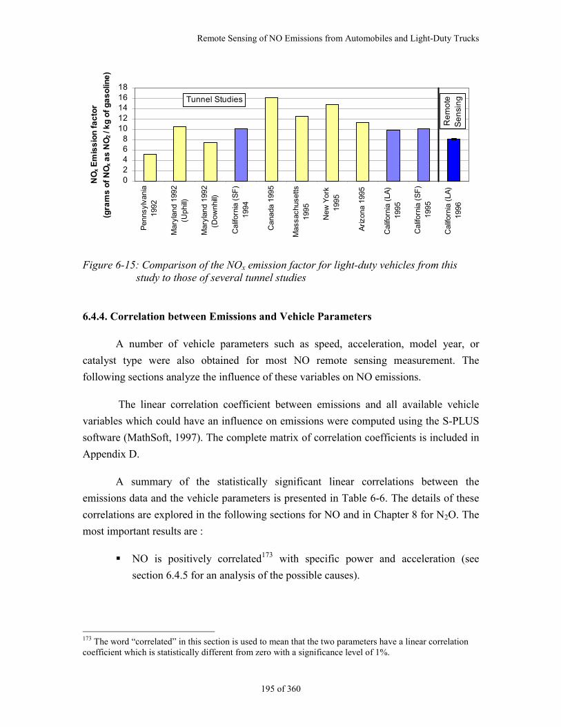
Remote Sensing of NO Emissions from Automobiles and Light-Duty Trucks

195 of 360

02468

1012141618

Pen

nsyl

vani

a19

92

Mar

ylan

d 19

92(U

phill)

Mar

ylan

d 19

92(D

ownh

ill)

Cal

iforn

ia (

SF

)19

94

Can

ada

1995

Mas

sach

uset

ts19

95

New

Yor

k19

95

Ariz

ona

1995

Cal

iforn

ia (

LA)

1995

Cal

iforn

ia (

SF

)19

95

Cal

iforn

ia (

LA)

1996

NO

x E

mis

sio

n f

ac

tor

(gra

ms

of

NO

x a

s N

O2

/ kg

of

ga

so

line

)Tunnel Studies

Re

mo

teS

en

sin

g

Figure 6-15: Comparison of the NOx emission factor for light-duty vehicles from thisstudy to those of several tunnel studies

6.4.4. Correlation between Emissions and Vehicle Parameters

A number of vehicle parameters such as speed, acceleration, model year, or

catalyst type were also obtained for most NO remote sensing measurement. The

following sections analyze the influence of these variables on NO emissions.

The linear correlation coefficient between emissions and all available vehicle

variables which could have an influence on emissions were computed using the S-PLUS

software (MathSoft, 1997). The complete matrix of correlation coefficients is included in

Appendix D.

A summary of the statistically significant linear correlations between the

emissions data and the vehicle parameters is presented in Table 6-6. The details of these

correlations are explored in the following sections for NO and in Chapter 8 for N2O. The

most important results are :

NO is positively correlated173 with specific power and acceleration (see

section 6.4.5 for an analysis of the possible causes).

173 The word “correlated” in this section is used to mean that the two parameters have a linear correlationcoefficient which is statistically different from zero with a significance level of 1%.

Chapter 6

196 of 360

NO is negatively correlated with the presence of a three-way catalyst and

positively with an oxidation catalyst. This can be expected since only three-

way catalysts are designed to reduce NOx emissions.

HC is negatively correlated with specific power (see Figure 3-35). This can be

explained by the increased HC emissions under sudden or prolonged

decelerations (see discussion in section 3.2.2).

CO and N2O are positively correlated with acceleration but not with specific

power. This is an artifact of the calculation procedure: both emissions increase

with specific power but in a non-linear fashion (see Figure 3-33 for CO and

Figure 8-20 for N2O) and acceleration can be thought of as a “blurred”

specific power (see Figure 6-10) which “diffuses” some of the non-linearities

of the physical response.

NO, CO, and HC are negatively correlated with vehicle model year (i.e.

positively correlated with vehicle age (section 6.4.9). This has been previously

reported in the literature (Zhang et al., 1993; Zhang et al., 1996a; Stedman et

al., 1997a), and is explained by less stringent emission standards and

increased deterioration for older vehicles.

NO N2O CO HC Speed Acc. SP MY Disp TWC OXY EGR CAR LDT USA

NO ↑ ↑ ↑ ↓ ↓ ↑ ↓ ↓N2O ↓ ↑CO ↑ ↑ ↑ ↓HC ↑ ↓ ↓

Table 6-6: Statistically significant correlations (α=1%)174 between emissions and vehicleparameters175

NO and N2O are positively correlated due to the formation process of N2O in

the catalyst (see the experimental results in section 8.3.7 and a model of this

process in section 8.4.1).

174 As determined by the test on p. 636 of Press et al. (Press et al., 1992), which does not require theassumption of a particular statistical distribution. The level of significance was α=1%. Note that this is thecoefficient of linear correlation and may not capture non-linear relationships between the variables.175 Key to the labels: Acc: acceleration; SP: specific power; MY: model year; Disp: engine displacement;TWC: vehicle equipped with three way catalyst; OXY: oxidation catalyst; EGR: exhaust gas recirculation;CAR: passenger car; LDT: light-duty truck; USA: manufactured in the USA.

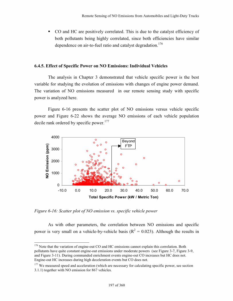
Remote Sensing of NO Emissions from Automobiles and Light-Duty Trucks

197 of 360

CO and HC are positively correlated. This is due to the catalyst efficiency of

both pollutants being highly correlated, since both efficiencies have similar

dependence on air-to-fuel ratio and catalyst degradation.176

6.4.5. Effect of Specific Power on NO Emissions: Individual Vehicles

The analysis in Chapter 3 demonstrated that vehicle specific power is the best

variable for studying the evolution of emissions with changes of engine power demand.

The variation of NO emissions measured in our remote sensing study with specific

power is analyzed here.

Figure 6-16 presents the scatter plot of NO emissions versus vehicle specific

power and Figure 6-22 shows the average NO emissions of each vehicle population

decile rank ordered by specific power.177

0

1000

2000

3000

4000

-10.0 0.0 10.0 20.0 30.0 40.0 50.0 60.0 70.0

Total Specific Power (kW / Metric Ton)

NO

Em

issi

on

(p

pm

)

Beyond FTP

Figure 6-16: Scatter plot of NO emission vs. specific vehicle power

As with other parameters, the correlation between NO emissions and specific

power is very small on a vehicle-by-vehicle basis (R2 = 0.023). Although the results in

176 Note that the variation of engine-out CO and HC emissions cannot explain this correlation. Bothpollutants have quite constant engine-out emissions under moderate powers (see Figure 3-7, Figure 3-9,and Figure 3-11). During commanded enrichment events engine-out CO increases but HC does not.Engine-out HC increases during high deceleration events but CO does not.177 We measured speed and acceleration (which are necessary for calculating specific power, see section3.1.1) together with NO emission for 867 vehicles.

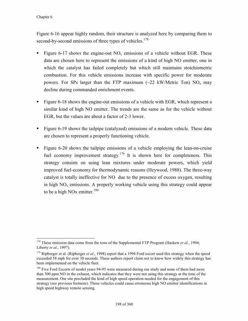
Chapter 6

198 of 360

Figure 6-16 appear highly random, their structure is analyzed here by comparing them to

second-by-second emissions of three types of vehicles.178

Figure 6-17 shows the engine-out NOx emissions of a vehicle without EGR. These

data are chosen here to represent the emissions of a kind of high NO emitter, one in

which the catalyst has failed completely but which still maintains stoichiometric

combustion. For this vehicle emissions increase with specific power for moderate

powers. For SPs larger than the FTP maximum (~22 kW/Metric Ton) NOx may

decline during commanded enrichment events.

Figure 6-18 shows the engine-out emissions of a vehicle with EGR, which represent a

similar kind of high NO emitter. The trends are the same as for the vehicle without

EGR, but the values are about a factor of 2-3 lower.

Figure 6-19 shows the tailpipe (catalyzed) emissions of a modern vehicle. These data

are chosen to represent a properly functioning vehicle.

Figure 6-20 shows the tailpipe emissions of a vehicle employing the lean-on-cruise

fuel economy improvement strategy.179 It is shown here for completeness. This

strategy consists on using lean mixtures under moderate powers, which yield

improved fuel-economy for thermodynamic reasons (Heywood, 1988). The three-way

catalyst is totally ineffective for NO due to the presence of excess oxygen, resulting

in high NOx emissions. A properly working vehicle using this strategy could appear

to be a high NOx emitter.180

178 These emission data come from the tests of the Supplemental FTP Program (Haskew et al., 1994;Liberty et al., 1997).179 Ripberger et al. (Ripberger et al., 1998) report that a 1994 Ford escort used this strategy when the speedexceeded 58 mph for over 30 seconds. These authors report claim not to know how widely this strategy hasbeen implemented on the vehicle fleet.180 Five Ford Escorts of model years 94-95 were measured during our study and none of them had morethan 300 ppm NO in the exhaust, which indicates that they were not using this strategy at the time of themeasurement. Our site precluded the kind of high speed operation needed for the engagement of thisstrategy (see previous footnote). These vehicles could cause erroneous high NO emitter identifications inhigh speed highway remote sensing.

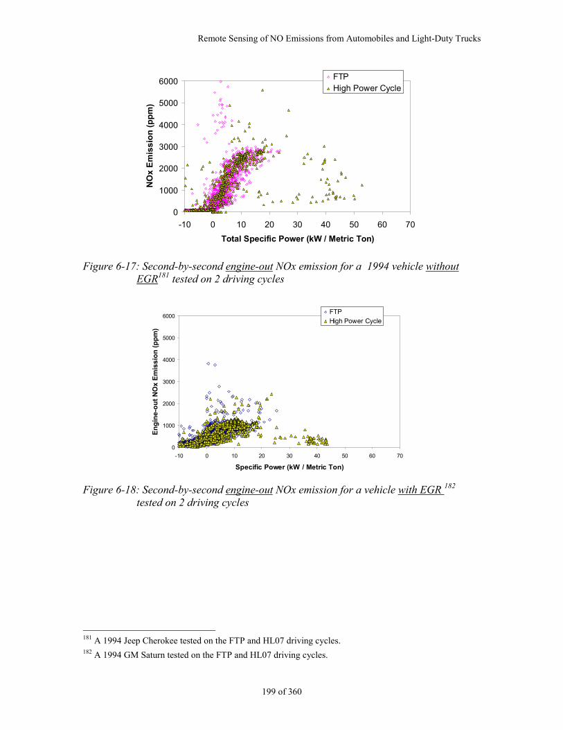
Remote Sensing of NO Emissions from Automobiles and Light-Duty Trucks

199 of 360

0

1000

2000

3000

4000

5000

6000

-10 0 10 20 30 40 50 60 70

Total Specific Power (kW / Metric Ton)

NO

x E

mis

sio

n (

pp

m)

FTPHigh Power Cycle

Figure 6-17: Second-by-second engine-out NOx emission for a 1994 vehicle withoutEGR181 tested on 2 driving cycles

0

1000

2000

3000

4000

5000

6000

-10 0 10 20 30 40 50 60 70

Specific Power (kW / Metric Ton)

En

gin

e-o

ut

NO

x E

mis

sio

n (

pp

m)

FTP

High Power Cycle

Figure 6-18: Second-by-second engine-out NOx emission for a vehicle with EGR 182

tested on 2 driving cycles

181 A 1994 Jeep Cherokee tested on the FTP and HL07 driving cycles.182 A 1994 GM Saturn tested on the FTP and HL07 driving cycles.

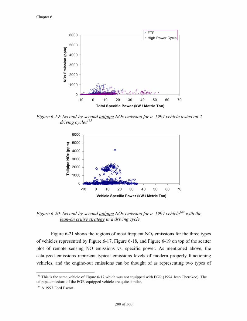
Chapter 6

200 of 360

0

1000

2000

3000

4000

5000

6000

-10 0 10 20 30 40 50 60 70

Total Specific Power (kW / Metric Ton)

NO

x E

mis

sio

n (

pp

m)

FTP

High Power Cycle

Figure 6-19: Second-by-second tailpipe NOx emission for a 1994 vehicle tested on 2driving cycles183

0

1000

2000

3000

4000

5000

6000

-10 0 10 20 30 40 50 60 70

Vehicle Specific Power (kW / Metric Ton)

Ta

ilp

ipe

NO

x (

pp

m)

Figure 6-20: Second-by-second tailpipe NOx emission for a 1994 vehicle184 with thelean-on cruise strategy in a driving cycle

Figure 6-21 shows the regions of most frequent NOx emissions for the three types

of vehicles represented by Figure 6-17, Figure 6-18, and Figure 6-19 on top of the scatter

plot of remote sensing NO emissions vs. specific power. As mentioned above, the

catalyzed emissions represent typical emissions levels of modern properly functioning

vehicles, and the engine-out emissions can be thought of as representing two types of

183 This is the same vehicle of Figure 6-17 which was not equipped with EGR (1994 Jeep Cherokee). Thetailpipe emissions of the EGR-equipped vehicle are quite similar.184 A 1993 Ford Escort.

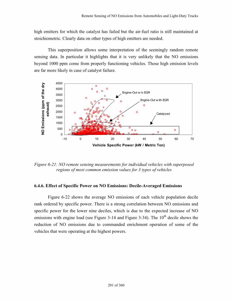
Remote Sensing of NO Emissions from Automobiles and Light-Duty Trucks

201 of 360

high emitters for which the catalyst has failed but the air-fuel ratio is still maintained at

stoichiometric. Clearly data on other types of high emitters are needed.

This superposition allows some interpretation of the seemingly random remote

sensing data. In particular it highlights that it is very unlikely that the NO emissions

beyond 1000 ppm come from properly functioning vehicles. Those high emission levels

are far more likely in case of catalyst failure.

0

500

1000

1500

2000

2500

3000

3500

4000

4500

-10 0 10 20 30 40 50 60 70

Vehicle Specific Power (kW / Metric Ton)

NO

Em

issi

on

s (p

pm

of

the

dry

exh

aust

)

Engine-Out w /o EGR

Catalyzed

Engine-Out w ith EGR

Figure 6-21: NO remote sensing measurements for individual vehicles with superposedregions of most common emission values for 3 types of vehicles

6.4.6. Effect of Specific Power on NO Emissions: Decile-Averaged Emissions

Figure 6-22 shows the average NO emissions of each vehicle population decile

rank ordered by specific power. There is a strong correlation between NO emissions and

specific power for the lower nine deciles, which is due to the expected increase of NO

emissions with engine load (see Figure 3-14 and Figure 3-34). The 10th decile shows the

reduction of NO emissions due to commanded enrichment operation of some of the

vehicles that were operating at the highest powers.

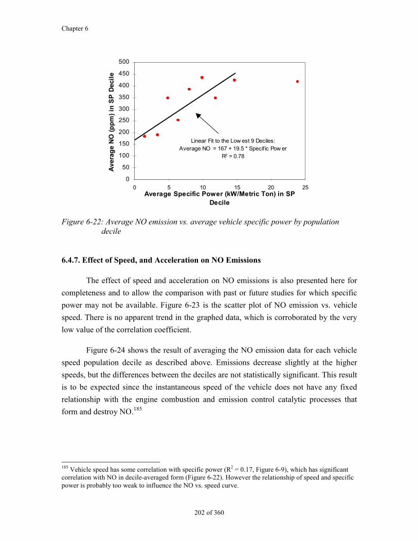
Chapter 6

202 of 360

0

50

100

150

200

250

300

350

400

450

500

0 5 10 15 20 25Average Specific Power (kW/Metric Ton) in SP

Decile

Ave

rag

e N

O (

pp

m)

in S

P D

ecil

e

Linear Fit to the Low est 9 Deciles:Average NO = 167 + 19.5 * Specif ic Pow er

R2 = 0.78

Figure 6-22: Average NO emission vs. average vehicle specific power by populationdecile

6.4.7. Effect of Speed, and Acceleration on NO Emissions

The effect of speed and acceleration on NO emissions is also presented here for

completeness and to allow the comparison with past or future studies for which specific

power may not be available. Figure 6-23 is the scatter plot of NO emission vs. vehicle

speed. There is no apparent trend in the graphed data, which is corroborated by the very

low value of the correlation coefficient.

Figure 6-24 shows the result of averaging the NO emission data for each vehicle

speed population decile as described above. Emissions decrease slightly at the higher

speeds, but the differences between the deciles are not statistically significant. This result

is to be expected since the instantaneous speed of the vehicle does not have any fixed

relationship with the engine combustion and emission control catalytic processes that

form and destroy NO.185

185 Vehicle speed has some correlation with specific power (R2 = 0.17, Figure 6-9), which has significantcorrelation with NO in decile-averaged form (Figure 6-22). However the relationship of speed and specificpower is probably too weak to influence the NO vs. speed curve.

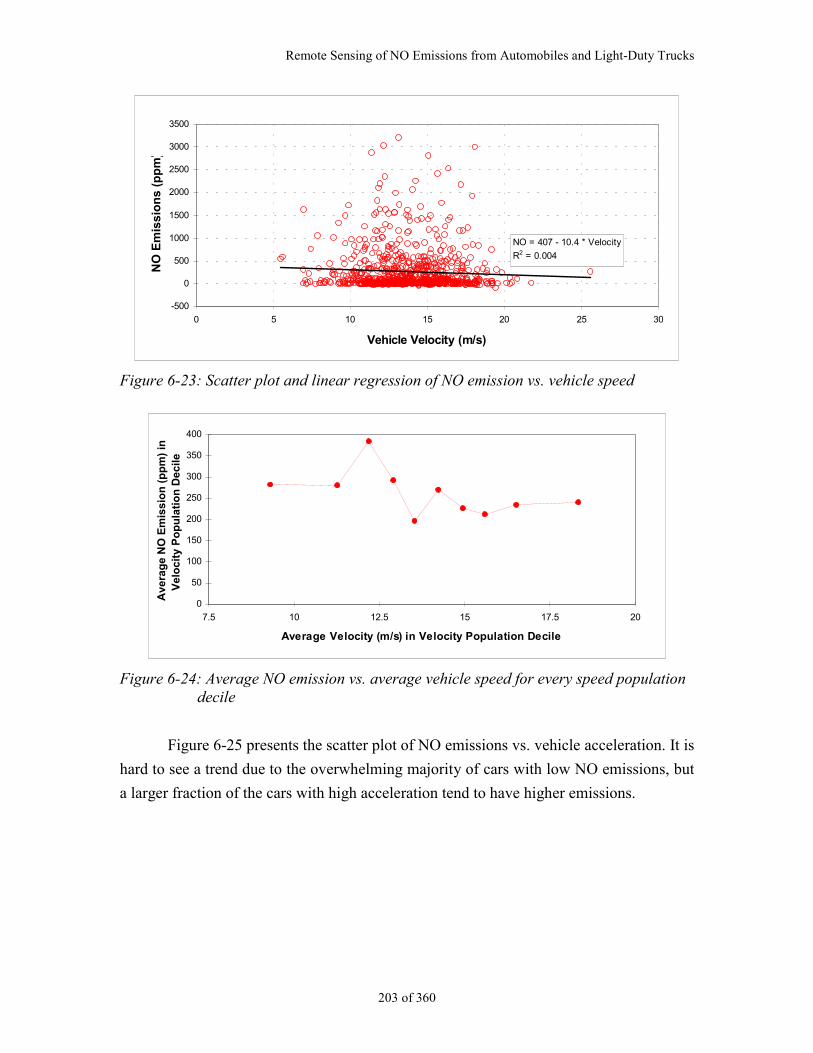
Remote Sensing of NO Emissions from Automobiles and Light-Duty Trucks

203 of 360

NO = 407 - 10.4 * Velocity

R2 = 0.004

-500

0

500

1000

1500

2000

2500

3000

3500

0 5 10 15 20 25 30

Vehicle Velocity (m/s)

NO

Em

issi

on

s (p

pm

)

Figure 6-23: Scatter plot and linear regression of NO emission vs. vehicle speed

0

50

100

150

200

250

300

350

400

7.5 10 12.5 15 17.5 20

Average Velocity (m/s) in Velocity Population Decile

Ave

rag

e N

O E

mis

sio

n (

pp

m)

in

Vel

oci

ty P

op

ula

tio

n D

ecile

Figure 6-24: Average NO emission vs. average vehicle speed for every speed populationdecile

Figure 6-25 presents the scatter plot of NO emissions vs. vehicle acceleration. It is

hard to see a trend due to the overwhelming majority of cars with low NO emissions, but

a larger fraction of the cars with high acceleration tend to have higher emissions.

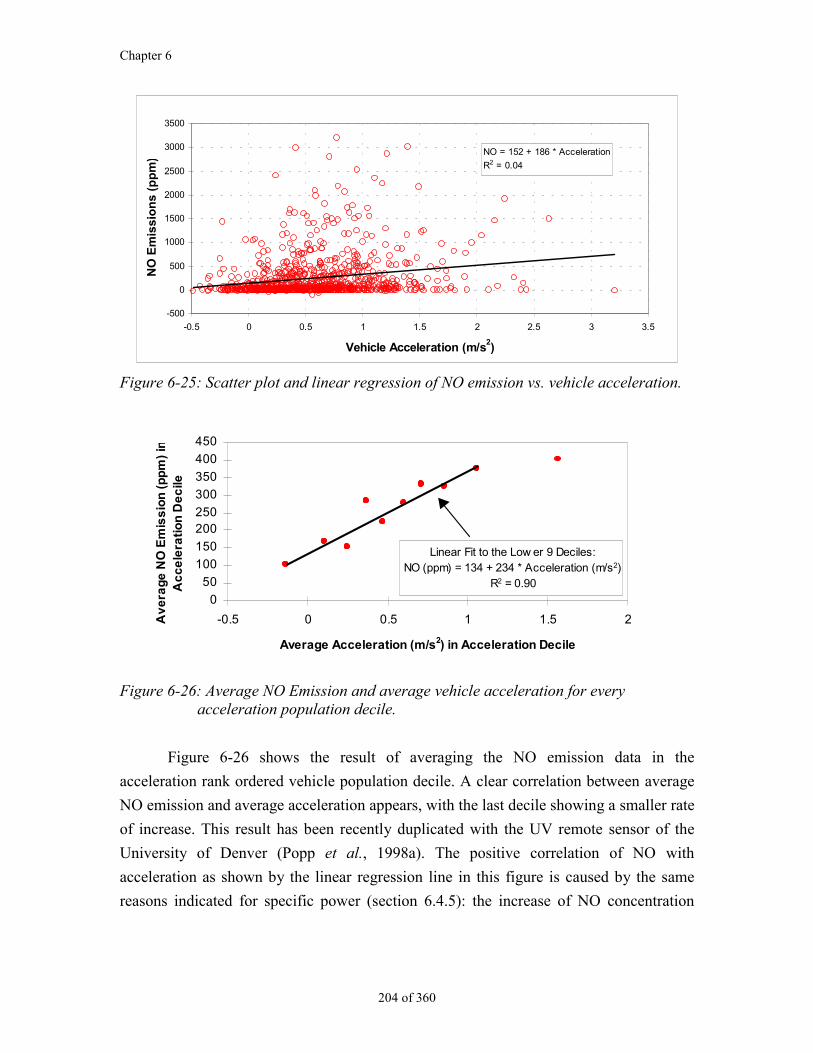
Chapter 6

204 of 360

NO = 152 + 186 * Acceleration

R2 = 0.04

-500

0

500

1000

1500

2000

2500

3000

3500

-0.5 0 0.5 1 1.5 2 2.5 3 3.5

Vehicle Acceleration (m/s2)

NO

Em

issi

on

s (p

pm

)

Figure 6-25: Scatter plot and linear regression of NO emission vs. vehicle acceleration.

Linear Fit to the Low er 9 Deciles:NO (ppm) = 134 + 234 * Acceleration (m/s2)

R2 = 0.90

0

50

100

150

200250

300

350

400

450

-0.5 0 0.5 1 1.5 2

Average Acceleration (m/s2) in Acceleration Decile

Av

era

ge

NO

Em

iss

ion

(p

pm

) in

Ac

ce

lera

tio

n D

ec

ile

Figure 6-26: Average NO Emission and average vehicle acceleration for everyacceleration population decile.

Figure 6-26 shows the result of averaging the NO emission data in the

acceleration rank ordered vehicle population decile. A clear correlation between average

NO emission and average acceleration appears, with the last decile showing a smaller rate

of increase. This result has been recently duplicated with the UV remote sensor of the

University of Denver (Popp et al., 1998a). The positive correlation of NO with

acceleration as shown by the linear regression line in this figure is caused by the same

reasons indicated for specific power (section 6.4.5): the increase of NO concentration

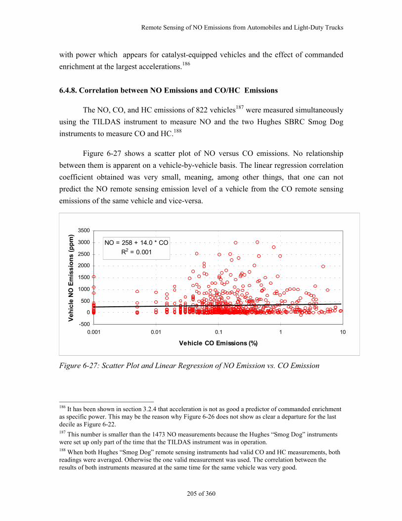
Remote Sensing of NO Emissions from Automobiles and Light-Duty Trucks

205 of 360

with power which appears for catalyst-equipped vehicles and the effect of commanded

enrichment at the largest accelerations.186

6.4.8. Correlation between NO Emissions and CO/HC Emissions

The NO, CO, and HC emissions of 822 vehicles187 were measured simultaneously

using the TILDAS instrument to measure NO and the two Hughes SBRC Smog Dog

instruments to measure CO and HC.188

Figure 6-27 shows a scatter plot of NO versus CO emissions. No relationship

between them is apparent on a vehicle-by-vehicle basis. The linear regression correlation

coefficient obtained was very small, meaning, among other things, that one can not

predict the NO remote sensing emission level of a vehicle from the CO remote sensing

emissions of the same vehicle and vice-versa.

NO = 258 + 14.0 * CO

R2 = 0.001

-500

0

500

1000

1500

2000

2500

3000

3500

0.001 0.01 0.1 1 10

Vehicle CO Emissions (%)

Veh

icle

NO

Em

issi

on

s (p

pm

)

Figure 6-27: Scatter Plot and Linear Regression of NO Emission vs. CO Emission

186 It has been shown in section 3.2.4 that acceleration is not as good a predictor of commanded enrichmentas specific power. This may be the reason why Figure 6-26 does not show as clear a departure for the lastdecile as Figure 6-22.187 This number is smaller than the 1473 NO measurements because the Hughes “Smog Dog” instrumentswere set up only part of the time that the TILDAS instrument was in operation.188 When both Hughes “Smog Dog” remote sensing instruments had valid CO and HC measurements, bothreadings were averaged. Otherwise the one valid measurement was used. The correlation between theresults of both instruments measured at the same time for the same vehicle was very good.

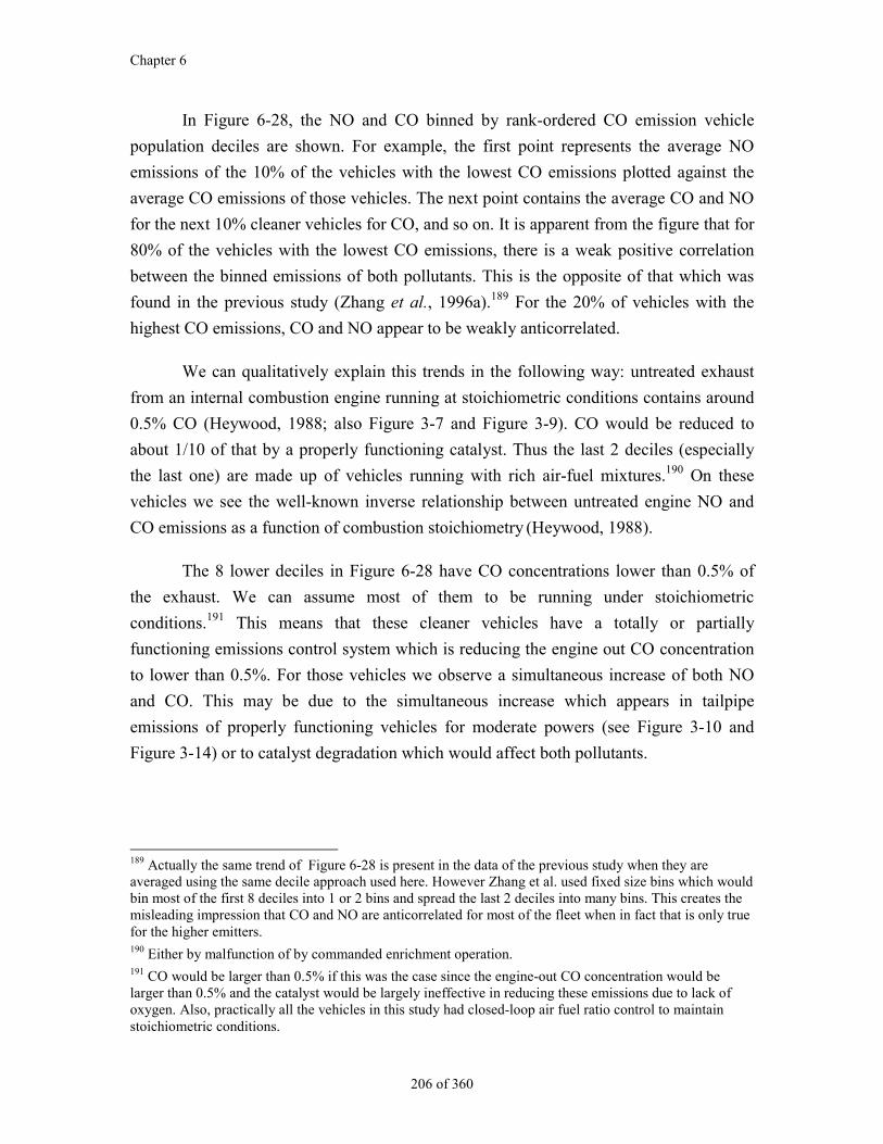
Chapter 6

206 of 360

In Figure 6-28, the NO and CO binned by rank-ordered CO emission vehicle

population deciles are shown. For example, the first point represents the average NO

emissions of the 10% of the vehicles with the lowest CO emissions plotted against the

average CO emissions of those vehicles. The next point contains the average CO and NO

for the next 10% cleaner vehicles for CO, and so on. It is apparent from the figure that for

80% of the vehicles with the lowest CO emissions, there is a weak positive correlation

between the binned emissions of both pollutants. This is the opposite of that which was

found in the previous study (Zhang et al., 1996a).189 For the 20% of vehicles with the

highest CO emissions, CO and NO appear to be weakly anticorrelated.

We can qualitatively explain this trends in the following way: untreated exhaust

from an internal combustion engine running at stoichiometric conditions contains around

0.5% CO (Heywood, 1988; also Figure 3-7 and Figure 3-9). CO would be reduced to

about 1/10 of that by a properly functioning catalyst. Thus the last 2 deciles (especially

the last one) are made up of vehicles running with rich air-fuel mixtures.190 On these

vehicles we see the well-known inverse relationship between untreated engine NO and

CO emissions as a function of combustion stoichiometry (Heywood, 1988).

The 8 lower deciles in Figure 6-28 have CO concentrations lower than 0.5% of

the exhaust. We can assume most of them to be running under stoichiometric

conditions.191 This means that these cleaner vehicles have a totally or partially

functioning emissions control system which is reducing the engine out CO concentration

to lower than 0.5%. For those vehicles we observe a simultaneous increase of both NO

and CO. This may be due to the simultaneous increase which appears in tailpipe

emissions of properly functioning vehicles for moderate powers (see Figure 3-10 and

Figure 3-14) or to catalyst degradation which would affect both pollutants.

189 Actually the same trend of Figure 6-28 is present in the data of the previous study when they areaveraged using the same decile approach used here. However Zhang et al. used fixed size bins which wouldbin most of the first 8 deciles into 1 or 2 bins and spread the last 2 deciles into many bins. This creates themisleading impression that CO and NO are anticorrelated for most of the fleet when in fact that is only truefor the higher emitters.190 Either by malfunction of by commanded enrichment operation.191 CO would be larger than 0.5% if this was the case since the engine-out CO concentration would belarger than 0.5% and the catalyst would be largely ineffective in reducing these emissions due to lack ofoxygen. Also, practically all the vehicles in this study had closed-loop air fuel ratio control to maintainstoichiometric conditions.

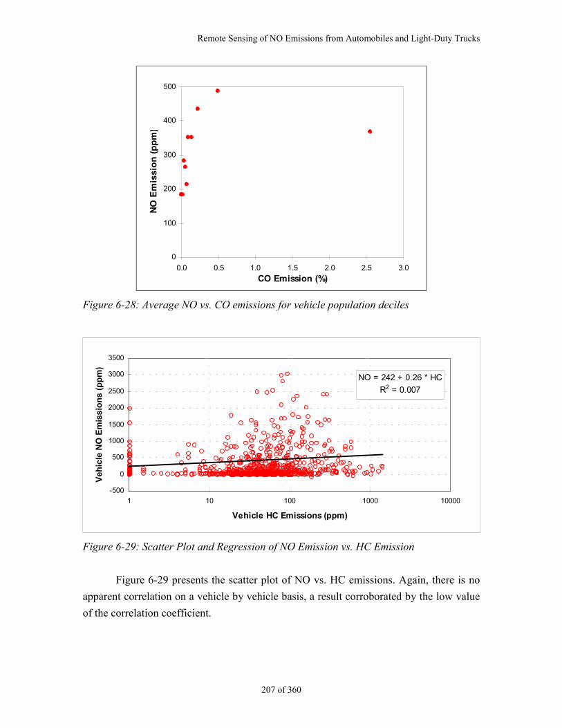
Remote Sensing of NO Emissions from Automobiles and Light-Duty Trucks

207 of 360

0

100

200

300

400

500

0.0 0.5 1.0 1.5 2.0 2.5 3.0

CO Emission (%)

NO

Em

issi

on

(p

pm

)

Figure 6-28: Average NO vs. CO emissions for vehicle population deciles

NO = 242 + 0.26 * HC

R2 = 0.007

-500

0

500

1000

1500

2000

2500

3000

3500

1 10 100 1000 10000

Vehicle HC Emissions (ppm)

Veh

icle

NO

Em

issi

on

s (p

pm

)

Figure 6-29: Scatter Plot and Regression of NO Emission vs. HC Emission

Figure 6-29 presents the scatter plot of NO vs. HC emissions. Again, there is no

apparent correlation on a vehicle by vehicle basis, a result corroborated by the low value

of the correlation coefficient.

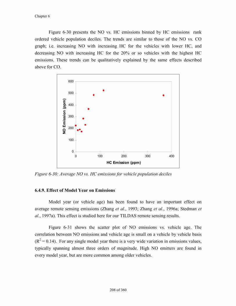
Chapter 6

208 of 360

Figure 6-30 presents the NO vs. HC emissions binned by HC emissions rank

ordered vehicle population deciles. The trends are similar to those of the NO vs. CO

graph; i.e. increasing NO with increasing HC for the vehicles with lower HC, and

decreasing NO with increasing HC for the 20% or so vehicles with the highest HC

emissions. These trends can be qualitatively explained by the same effects described

above for CO.

0

100

200

300

400

500

600

0 100 200 300 400

HC Emission (ppm)

NO

Em

issi

on

(p

pm

)

Figure 6-30: Average NO vs. HC emissions for vehicle population deciles

6.4.9. Effect of Model Year on Emissions

Model year (or vehicle age) has been found to have an important effect on

average remote sensing emissions (Zhang et al., 1993; Zhang et al., 1996a; Stedman et

al., 1997a). This effect is studied here for our TILDAS remote sensing results.

Figure 6-31 shows the scatter plot of NO emissions vs. vehicle age. The

correlation between NO emissions and vehicle age is small on a vehicle by vehicle basis

(R2 = 0.14). For any single model year there is a very wide variation in emissions values,

typically spanning almost three orders of magnitude. High NO emitters are found in

every model year, but are more common among older vehicles.

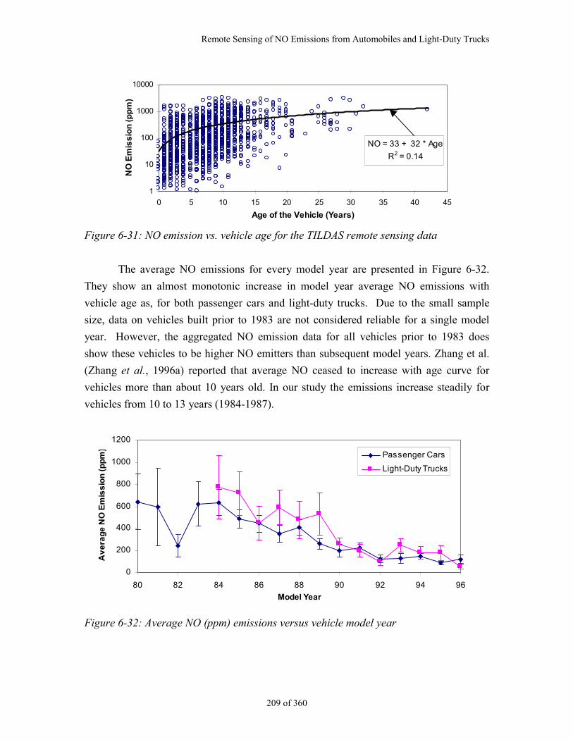
Remote Sensing of NO Emissions from Automobiles and Light-Duty Trucks

209 of 360

NO = 33 + 32 * Age

R2 = 0.14

1

10

100

1000

10000

0 5 10 15 20 25 30 35 40 45

Age of the Vehicle (Years)

NO

Em

iss

ion

(p

pm

)

Figure 6-31: NO emission vs. vehicle age for the TILDAS remote sensing data

The average NO emissions for every model year are presented in Figure 6-32.

They show an almost monotonic increase in model year average NO emissions with

vehicle age as, for both passenger cars and light-duty trucks. Due to the small sample

size, data on vehicles built prior to 1983 are not considered reliable for a single model

year. However, the aggregated NO emission data for all vehicles prior to 1983 does

show these vehicles to be higher NO emitters than subsequent model years. Zhang et al.

(Zhang et al., 1996a) reported that average NO ceased to increase with age curve for

vehicles more than about 10 years old. In our study the emissions increase steadily for

vehicles from 10 to 13 years (1984-1987).

0

200

400

600

800

1000

1200

80 82 84 86 88 90 92 94 96

Model Year

Av

era

ge

NO

Em

iss

ion

(p

pm

)

Passenger Cars

Light-Duty Trucks

Figure 6-32: Average NO (ppm) emissions versus vehicle model year

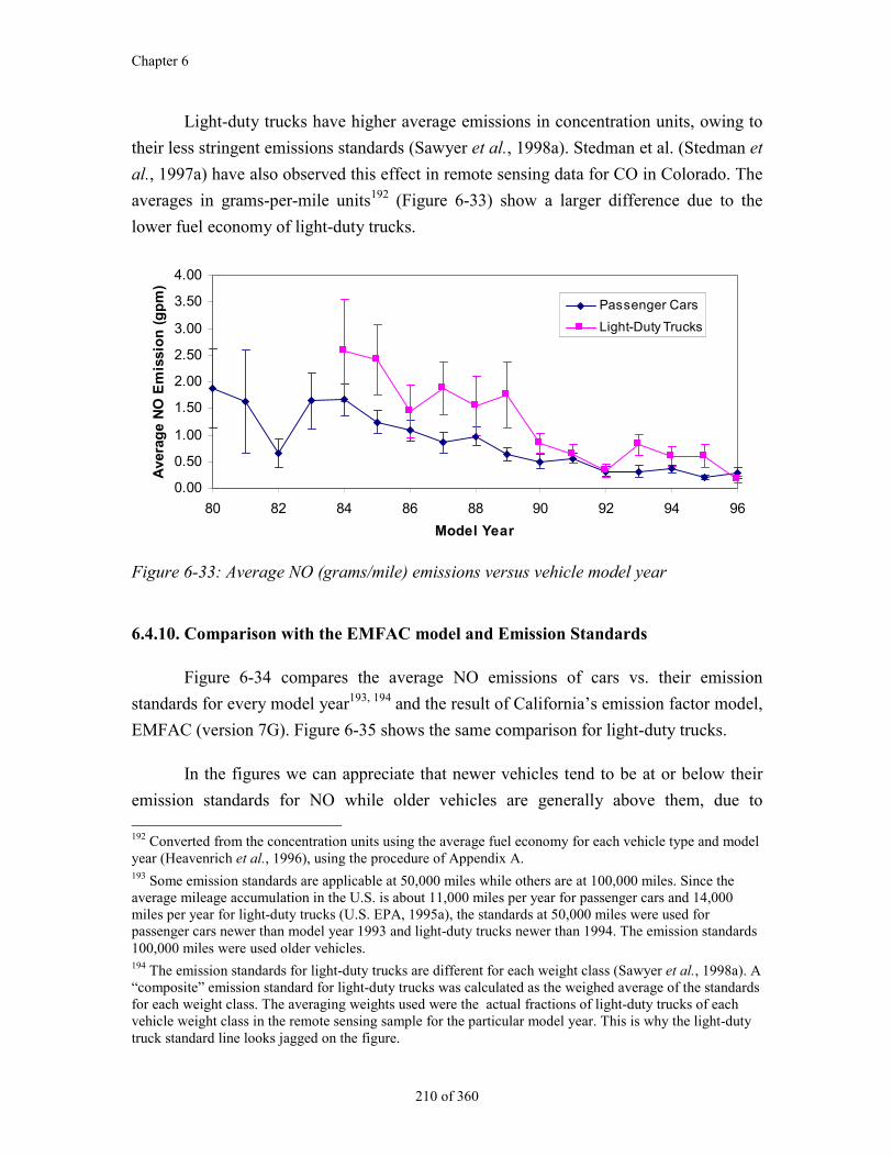
Chapter 6

210 of 360

Light-duty trucks have higher average emissions in concentration units, owing to

their less stringent emissions standards (Sawyer et al., 1998a). Stedman et al. (Stedman et

al., 1997a) have also observed this effect in remote sensing data for CO in Colorado. The

averages in grams-per-mile units192 (Figure 6-33) show a larger difference due to the

lower fuel economy of light-duty trucks.

0.00

0.50

1.00

1.50

2.00

2.50

3.00

3.50

4.00

80 82 84 86 88 90 92 94 96

Model Year

Ave

rag

e N

O E

mis

sio

n (

gp

m)

Passenger Cars

Light-Duty Trucks

Figure 6-33: Average NO (grams/mile) emissions versus vehicle model year

6.4.10. Comparison with the EMFAC model and Emission Standards

Figure 6-34 compares the average NO emissions of cars vs. their emission

standards for every model year193, 194 and the result of California’s emission factor model,

EMFAC (version 7G). Figure 6-35 shows the same comparison for light-duty trucks.

In the figures we can appreciate that newer vehicles tend to be at or below their

emission standards for NO while older vehicles are generally above them, due to 192 Converted from the concentration units using the average fuel economy for each vehicle type and modelyear (Heavenrich et al., 1996), using the procedure of Appendix A.193 Some emission standards are applicable at 50,000 miles while others are at 100,000 miles. Since theaverage mileage accumulation in the U.S. is about 11,000 miles per year for passenger cars and 14,000miles per year for light-duty trucks (U.S. EPA, 1995a), the standards at 50,000 miles were used forpassenger cars newer than model year 1993 and light-duty trucks newer than 1994. The emission standards100,000 miles were used older vehicles.194 The emission standards for light-duty trucks are different for each weight class (Sawyer et al., 1998a). A“composite” emission standard for light-duty trucks was calculated as the weighed average of the standardsfor each weight class. The averaging weights used were the actual fractions of light-duty trucks of eachvehicle weight class in the remote sensing sample for the particular model year. This is why the light-dutytruck standard line looks jagged on the figure.

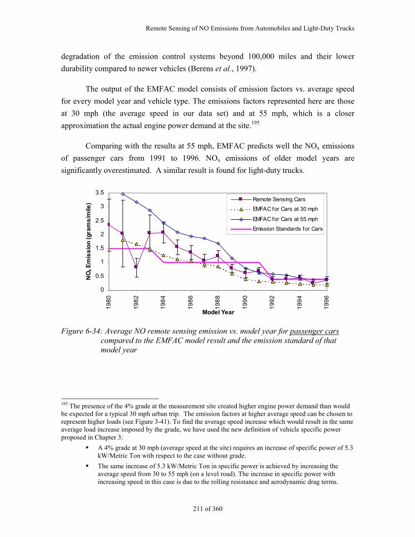
Remote Sensing of NO Emissions from Automobiles and Light-Duty Trucks

211 of 360

degradation of the emission control systems beyond 100,000 miles and their lower

durability compared to newer vehicles (Berens et al., 1997).

The output of the EMFAC model consists of emission factors vs. average speed

for every model year and vehicle type. The emissions factors represented here are those

at 30 mph (the average speed in our data set) and at 55 mph, which is a closer

approximation the actual engine power demand at the site.195

Comparing with the results at 55 mph, EMFAC predicts well the NOx emissions

of passenger cars from 1991 to 1996. NOx emissions of older model years are

significantly overestimated. A similar result is found for light-duty trucks.

0

0.5

1

1.5

2

2.5

3

3.5

19

80

19

82

19

84

19

86

19

88

19

90

19

92

19

94

19

96

Model Year

NO

x E

mis

sio

n (

gra

ms

/mile

)

Remote Sensing Cars

EMFAC for Cars at 30 mph

EMFAC for Cars at 55 mph

Emission Standards for Cars

Figure 6-34: Average NO remote sensing emission vs. model year for passenger carscompared to the EMFAC model result and the emission standard of thatmodel year

195 The presence of the 4% grade at the measurement site created higher engine power demand than wouldbe expected for a typical 30 mph urban trip. The emission factors at higher average speed can be chosen torepresent higher loads (see Figure 3-41). To find the average speed increase which would result in the sameaverage load increase imposed by the grade, we have used the new definition of vehicle specific powerproposed in Chapter 3:

A 4% grade at 30 mph (average speed at the site) requires an increase of specific power of 5.3kW/Metric Ton with respect to the case without grade.

The same increase of 5.3 kW/Metric Ton in specific power is achieved by increasing theaverage speed from 30 to 55 mph (on a level road). The increase in specific power withincreasing speed in this case is due to the rolling resistance and aerodynamic drag terms.

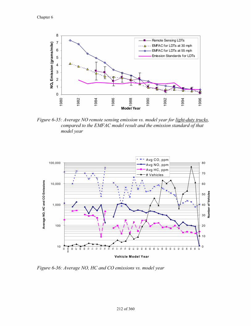
Chapter 6

212 of 360

0

1

2

3

4

5

6

7

8

19

80

19

82

19

84

19

86

19

88

19

90

19

92

19

94

19

96

Model Year

NO

x E

mis

sio

n (

gra

ms

/mile

) Remote Sensing LDTs

EMFAC for LDTs at 30 mph

EMFAC for LDTs at 55 mph

Emission Standards for LDTs

Figure 6-35: Average NO remote sensing emission vs. model year for light-duty trucks,compared to the EMFAC model result and the emission standard of thatmodel year

10

100

1,000

10,000

100,000

55

56

-65

66

67

68

69

70

71

72

73

74

75

76

77

78

79

80

81

82

83

84

85

86

87

88

89

90

91

92

93

94

95

96

97

Vehicle Model Year

Ave

rag

e N

O, H

C a

nd

CO

Em

issi

on

s

0

10

20

30

40

50

60

70

80

Nu

mb

er o

f V

ehic

les

Avg CO, ppm

Avg NO, ppm

Avg HC, ppm

# Vehicles

Figure 6-36: Average NO, HC and CO emissions vs. model year

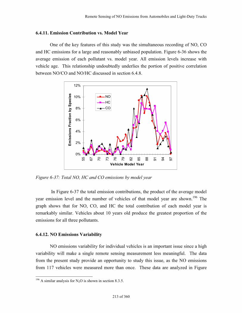
Remote Sensing of NO Emissions from Automobiles and Light-Duty Trucks

213 of 360

6.4.11. Emission Contribution vs. Model Year

One of the key features of this study was the simultaneous recording of NO, CO

and HC emissions for a large and reasonably unbiased population. Figure 6-36 shows the

average emission of each pollutant vs. model year. All emission levels increase with

vehicle age. This relationship undoubtedly underlies the portion of positive correlation

between NO/CO and NO/HC discussed in section 6.4.8.

0%

2%

4%

6%

8%

10%

12%55 67 70 73 76 79 82 85 88 91 94 97

Vehicle Model Year

Em

issi

on

s F

ract

ion

by

Sp

ecie

s

NO

HC

CO

Figure 6-37: Total NO, HC and CO emissions by model year

In Figure 6-37 the total emission contributions, the product of the average model

year emission level and the number of vehicles of that model year are shown.196 The

graph shows that for NO, CO, and HC the total contribution of each model year is

remarkably similar. Vehicles about 10 years old produce the greatest proportion of the

emissions for all three pollutants.

6.4.12. NO Emissions Variability

NO emissions variability for individual vehicles is an important issue since a high

variability will make a single remote sensing measurement less meaningful. The data

from the present study provide an opportunity to study this issue, as the NO emissions

from 117 vehicles were measured more than once. These data are analyzed in Figure

196 A similar analysis for N2O is shown in section 8.3.5.

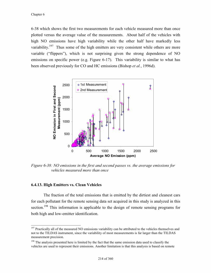
Chapter 6

214 of 360

6-38 which shows the first two measurements for each vehicle measured more than once

plotted versus the average value of the measurements. About half of the vehicles with

high NO emissions have high variability while the other half have markedly less

variability.197 Thus some of the high emitters are very consistent while others are more

variable (“flippers”), which is not surprising given the strong dependence of NO

emissions on specific power (e.g. Figure 6-17). This variability is similar to what has

been observed previously for CO and HC emissions (Bishop et al., 1996d).

0

500

1000

1500

2000

2500

0 500 1000 1500 2000 2500

Average NO Emission (ppm)

NO

Em

issi

on

in

Fir

st a

nd

Sec

on

dM

easu

rem

ent

(pp

m)

1st Measurement

2nd Measurement

Figure 6-38: NO emissions in the first and second passes vs. the average emissions forvehicles measured more than once

6.4.13. High Emitters vs. Clean Vehicles

The fraction of the total emissions that is emitted by the dirtiest and cleanest cars

for each pollutant for the remote sensing data set acquired in this study is analyzed in this

section.198 This information is applicable to the design of remote sensing programs for

both high and low-emitter identification.

197 Practically all of the measured NO emissions variability can be attributed to the vehicles themselves andnot to the TILDAS instrument, since the variability of most measurements is far larger than the TILDASmeasurement precision.198 The analysis presented here is limited by the fact that the same emission data used to classify thevehicles are used to represent their emissions. Another limitation is that this analysis is based on remote

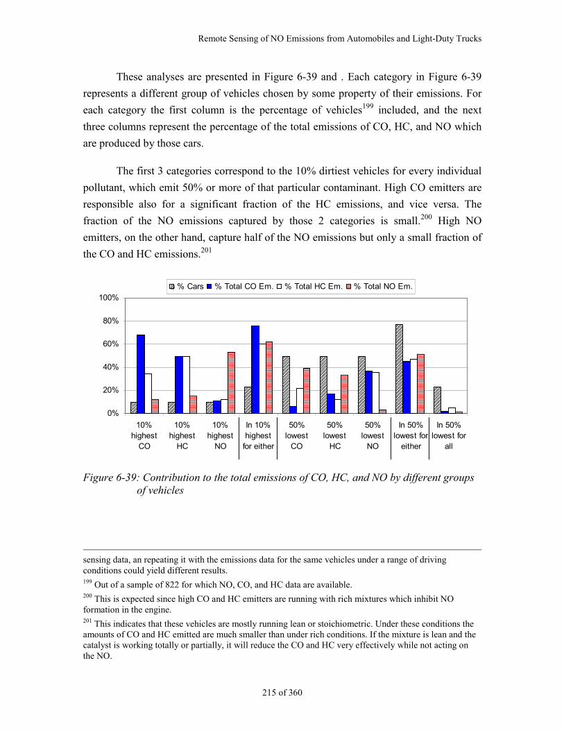
Remote Sensing of NO Emissions from Automobiles and Light-Duty Trucks

215 of 360

These analyses are presented in Figure 6-39 and . Each category in Figure 6-39

represents a different group of vehicles chosen by some property of their emissions. For

each category the first column is the percentage of vehicles199 included, and the next

three columns represent the percentage of the total emissions of CO, HC, and NO which

are produced by those cars.

The first 3 categories correspond to the 10% dirtiest vehicles for every individual

pollutant, which emit 50% or more of that particular contaminant. High CO emitters are

responsible also for a significant fraction of the HC emissions, and vice versa. The

fraction of the NO emissions captured by those 2 categories is small.200 High NO

emitters, on the other hand, capture half of the NO emissions but only a small fraction of

the CO and HC emissions.201

������������

����������������

����������

������������������������

��������������������������������������������������������

�����������������������������������

�������������������������������������������������

��������������������������������������������������������������������������������

��������������������

������������������

���������������������

�����������������������������������

������������������������������������������������

������������������������������������������������

�������������������������

������������

�������������������������������������������������������� �����0%

20%

40%

60%

80%

100%

10%highest

CO

10%highest

HC

10%highest

NO

In 10%highest

for either

50%lowest

CO

50%lowest

HC

50%lowest

NO

In 50%lowest for

either

In 50%lowest for

all

���% Cars % Total CO Em. % Total HC Em.

�������% Total NO Em.

Figure 6-39: Contribution to the total emissions of CO, HC, and NO by different groupsof vehicles

sensing data, an repeating it with the emissions data for the same vehicles under a range of drivingconditions could yield different results.199 Out of a sample of 822 for which NO, CO, and HC data are available.200 This is expected since high CO and HC emitters are running with rich mixtures which inhibit NOformation in the engine.201 This indicates that these vehicles are mostly running lean or stoichiometric. Under these conditions theamounts of CO and HC emitted are much smaller than under rich conditions. If the mixture is lean and thecatalyst is working totally or partially, it will reduce the CO and HC very effectively while not acting onthe NO.

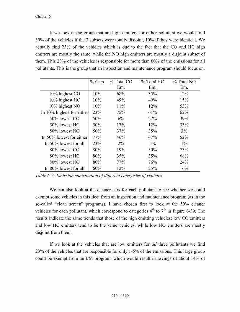
Chapter 6

216 of 360

If we look at the group that are high emitters for either pollutant we would find

30% of the vehicles if the 3 subsets were totally disjoint, 10% if they were identical. We

actually find 23% of the vehicles which is due to the fact that the CO and HC high

emitters are mostly the same, while the NO high emitters are mostly a disjoint subset of

them. This 23% of the vehicles is responsible for more than 60% of the emissions for all

pollutants. This is the group that an inspection and maintenance program should focus on.

% Cars % Total COEm.

% Total HCEm.

% Total NOEm.

10% highest CO 10% 68% 35% 12%10% highest HC 10% 49% 49% 15%10% highest NO 10% 11% 12% 53%

In 10% highest for either 23% 75% 61% 62%50% lowest CO 50% 6% 22% 39%50% lowest HC 50% 17% 12% 33%50% lowest NO 50% 37% 35% 3%

In 50% lowest for either 77% 46% 47% 52%In 50% lowest for all 23% 2% 5% 1%

80% lowest CO 80% 19% 50% 73%80% lowest HC 80% 35% 35% 68%80% lowest NO 80% 77% 76% 24%

In 80% lowest for all 60% 12% 25% 16%

Table 6-7: Emission contribution of different categories of vehicles

We can also look at the cleaner cars for each pollutant to see whether we could

exempt some vehicles in this fleet from an inspection and maintenance program (as in the

so-called “clean screen” programs). I have chosen first to look at the 50% cleaner

vehicles for each pollutant, which correspond to categories 4th to 7th in Figure 6-39. The

results indicate the same trends that those of the high emitting vehicles: low CO emitters

and low HC emitters tend to be the same vehicles, while low NO emitters are mostly

disjoint from them.

If we look at the vehicles that are low emitters for all three pollutants we find

23% of the vehicles that are responsible for only 1-5% of the emissions. This large group

could be exempt from an I/M program, which would result in savings of about 14% of

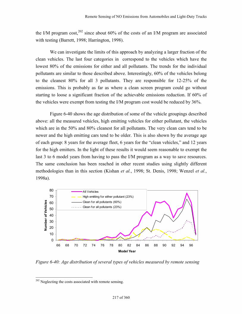
Remote Sensing of NO Emissions from Automobiles and Light-Duty Trucks

217 of 360

the I/M program cost,202 since about 60% of the costs of an I/M program are associated

with testing (Barrett, 1998; Harrington, 1998).

We can investigate the limits of this approach by analyzing a larger fraction of the

clean vehicles. The last four categories in correspond to the vehicles which have the

lowest 80% of the emissions for either and all pollutants. The trends for the individual

pollutants are similar to those described above. Interestingly, 60% of the vehicles belong

to the cleanest 80% for all 3 pollutants. They are responsible for 12-25% of the

emissions. This is probably as far as where a clean screen program could go without

starting to loose a significant fraction of the achievable emissions reduction. If 60% of

the vehicles were exempt from testing the I/M program cost would be reduced by 36%.

Figure 6-40 shows the age distribution of some of the vehicle groupings described

above: all the measured vehicles, high emitting vehicles for either pollutant, the vehicles

which are in the 50% and 80% cleanest for all pollutants. The very clean cars tend to be

newer and the high emitting cars tend to be older. This is also shown by the average age

of each group: 8 years for the average fleet, 6 years for the “clean vehicles,” and 12 years

for the high emitters. In the light of these results it would seem reasonable to exempt the

last 3 to 6 model years from having to pass the I/M program as a way to save resources.

The same conclusion has been reached in other recent studies using slightly different

methodologies than in this section (Kishan et al., 1998; St. Denis, 1998; Wenzel et al.,

1998a).

0

10

20

30

40

50

60

70

80

66 68 70 72 74 76 78 80 82 84 86 88 90 92 94 96

Model Year

Nu

mb

er

of

Ve

hic

les

All Vehicles

High emitting for either pollutant (23%)

Clean for all pollutants (60%)

Clean for all pollutants (23%)

Figure 6-40: Age distribution of several types of vehicles measured by remote sensing

202 Neglecting the costs associated with remote sensing.

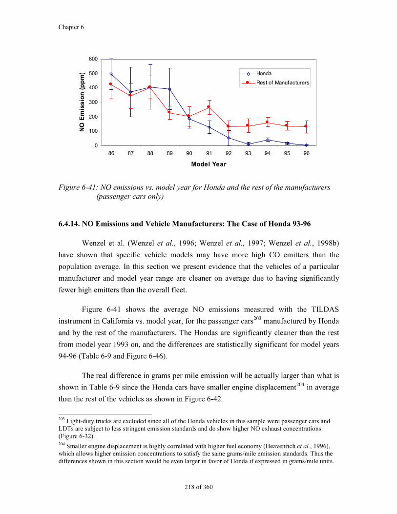
Chapter 6

218 of 360

0

100

200

300

400

500

600

86 87 88 89 90 91 92 93 94 95 96

Model Year

NO

Em

issi

on

(p

pm

) Honda

Rest of Manufacturers

Figure 6-41: NO emissions vs. model year for Honda and the rest of the manufacturers(passenger cars only)

6.4.14. NO Emissions and Vehicle Manufacturers: The Case of Honda 93-96

Wenzel et al. (Wenzel et al., 1996; Wenzel et al., 1997; Wenzel et al., 1998b)

have shown that specific vehicle models may have more high CO emitters than the

population average. In this section we present evidence that the vehicles of a particular

manufacturer and model year range are cleaner on average due to having significantly

fewer high emitters than the overall fleet.

Figure 6-41 shows the average NO emissions measured with the TILDAS

instrument in California vs. model year, for the passenger cars203 manufactured by Honda

and by the rest of the manufacturers. The Hondas are significantly cleaner than the rest

from model year 1993 on, and the differences are statistically significant for model years

94-96 (Table 6-9 and Figure 6-46).

The real difference in grams per mile emission will be actually larger than what is

shown in Table 6-9 since the Honda cars have smaller engine displacement204 in average

than the rest of the vehicles as shown in Figure 6-42.

203 Light-duty trucks are excluded since all of the Honda vehicles in this sample were passenger cars andLDTs are subject to less stringent emission standards and do show higher NO exhaust concentrations(Figure 6-32).204 Smaller engine displacement is highly correlated with higher fuel economy (Heavenrich et al., 1996),which allows higher emission concentrations to satisfy the same grams/mile emission standards. Thus thedifferences shown in this section would be even larger in favor of Honda if expressed in grams/mile units.

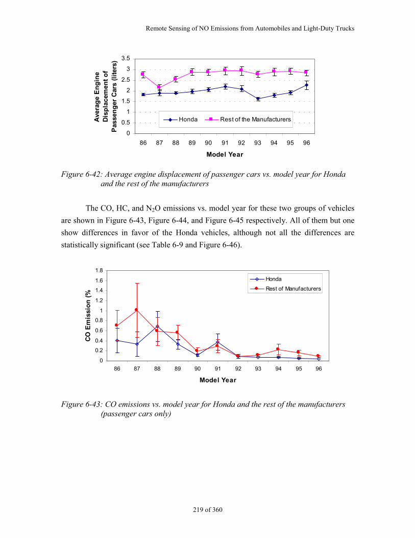
Remote Sensing of NO Emissions from Automobiles and Light-Duty Trucks

219 of 360

0

0.5

1

1.5

2

2.5

3

3.5

86 87 88 89 90 91 92 93 94 95 96

Model Year

Ave

rag

e E

ng

ine

Dis

pla

cem

ent

of

Pas

sen

ger

Car

s (l

iter

s)Honda Rest of the Manufacturers

Figure 6-42: Average engine displacement of passenger cars vs. model year for Hondaand the rest of the manufacturers

The CO, HC, and N2O emissions vs. model year for these two groups of vehicles

are shown in Figure 6-43, Figure 6-44, and Figure 6-45 respectively. All of them but one

show differences in favor of the Honda vehicles, although not all the differences are

statistically significant (see Table 6-9 and Figure 6-46).

0

0.2

0.4

0.6

0.8

1

1.2

1.4

1.6

1.8

86 87 88 89 90 91 92 93 94 95 96

Model Year

CO

Em

issi

on

(%

)

Honda

Rest of Manufacturers

Figure 6-43: CO emissions vs. model year for Honda and the rest of the manufacturers(passenger cars only)

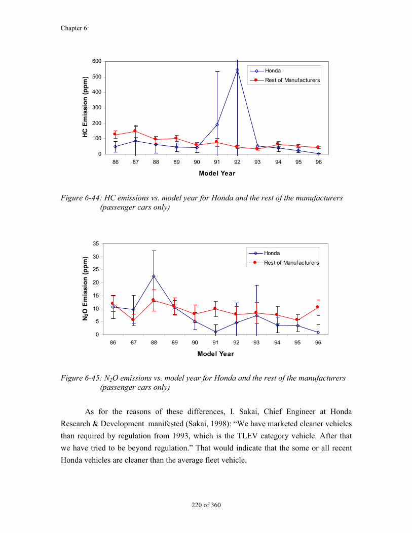
Chapter 6

220 of 360

0

100

200

300

400

500

600

86 87 88 89 90 91 92 93 94 95 96

Model Year

HC

Em

issi

on

(p

pm

)

Honda

Rest of Manufacturers

Figure 6-44: HC emissions vs. model year for Honda and the rest of the manufacturers(passenger cars only)

0

5

10

15

20

25

30

35

86 87 88 89 90 91 92 93 94 95 96

Model Year

N2O

Em

issi

on

(p

pm

)

Honda

Rest of Manufacturers

Figure 6-45: N2O emissions vs. model year for Honda and the rest of the manufacturers(passenger cars only)

As for the reasons of these differences, I. Sakai, Chief Engineer at Honda

Research & Development manifested (Sakai, 1998): “We have marketed cleaner vehicles

than required by regulation from 1993, which is the TLEV category vehicle. After that

we have tried to be beyond regulation.” That would indicate that the some or all recent

Honda vehicles are cleaner than the average fleet vehicle.

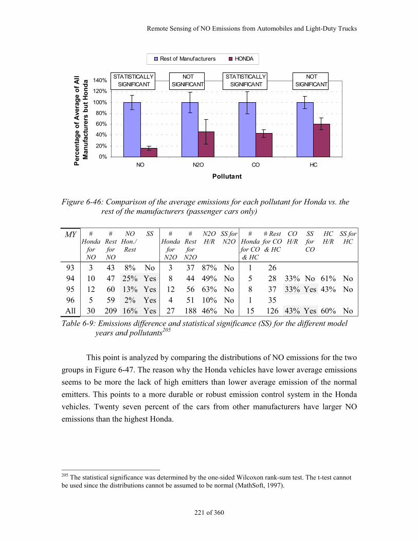
Remote Sensing of NO Emissions from Automobiles and Light-Duty Trucks

221 of 360

0%

20%

40%

60%

80%

100%

120%

140%

NO N2O CO HC

Pollutant

Per

cen

tag

e o

f A

vera

ge

of

All

M

anu

fact

ure

rs b

ut

Ho

nd

a

Rest of Manufacturers HONDA

STATISTICALLYSIGNIFICANT

STATISTICALLYSIGNIFICANT

NOTSIGNIFICANT

NOTSIGNIFICANT

Figure 6-46: Comparison of the average emissions for each pollutant for Honda vs. therest of the manufacturers (passenger cars only)

MY #Honda

forNO

#RestforNO

NOHon./Rest

SS #Honda

forN2O

#Restfor

N2O

N2OH/R

SS forN2O

#Hondafor CO& HC

# Restfor CO& HC

COH/R

SSforCO

HCH/R

SS forHC

93 3 43 8% No 3 37 87% No 1 2694 10 47 25% Yes 8 44 49% No 5 28 33% No 61% No95 12 60 13% Yes 12 56 63% No 8 37 33% Yes 43% No96 5 59 2% Yes 4 51 10% No 1 35All 30 209 16% Yes 27 188 46% No 15 126 43% Yes 60% No

Table 6-9: Emissions difference and statistical significance (SS) for the different modelyears and pollutants205

This point is analyzed by comparing the distributions of NO emissions for the two

groups in Figure 6-47. The reason why the Honda vehicles have lower average emissions

seems to be more the lack of high emitters than lower average emission of the normal

emitters. This points to a more durable or robust emission control system in the Honda

vehicles. Twenty seven percent of the cars from other manufacturers have larger NO

emissions than the highest Honda.

205 The statistical significance was determined by the one-sided Wilcoxon rank-sum test. The t-test cannotbe used since the distributions cannot be assumed to be normal (MathSoft, 1997).

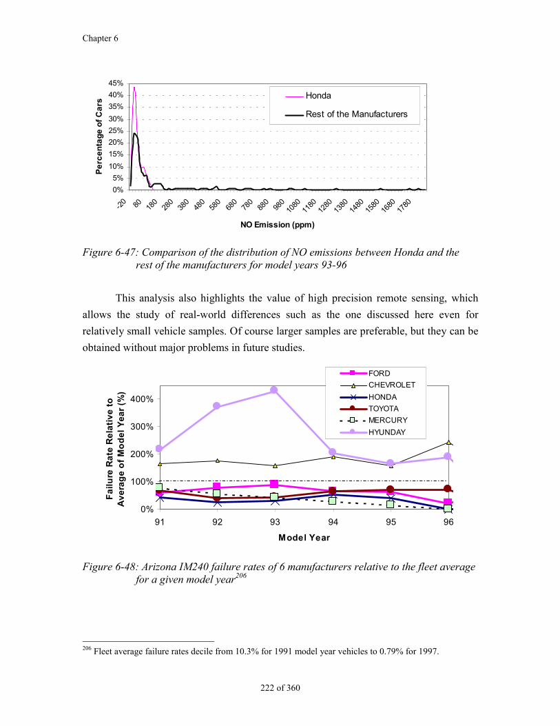
Chapter 6

222 of 360

0%

5%

10%

15%

20%

25%

30%

35%

40%

45%

-20 80 18

028

038

048

058

068

078

088

098

010

8011

8012

8013

8014

8015

8016

8017

80

NO Emission (ppm)

Pe

rce

nta

ge

of

Ca

rsHonda

Rest of the Manufacturers

Figure 6-47: Comparison of the distribution of NO emissions between Honda and therest of the manufacturers for model years 93-96

This analysis also highlights the value of high precision remote sensing, which

allows the study of real-world differences such as the one discussed here even for

relatively small vehicle samples. Of course larger samples are preferable, but they can be

obtained without major problems in future studies.

0%

100%

200%

300%

400%

91 92 93 94 95 96

Model Year

Fa

ilu

re R

ate

Re

lati

ve

to

A

ve

rag

e o

f M

od

el

Ye

ar

(%)

FORD

CHEVROLET

HONDA

TOYOTA

MERCURY

HYUNDAY

Figure 6-48: Arizona IM240 failure rates of 6 manufacturers relative to the fleet averagefor a given model year206

206 Fleet average failure rates decile from 10.3% for 1991 model year vehicles to 0.79% for 1997.

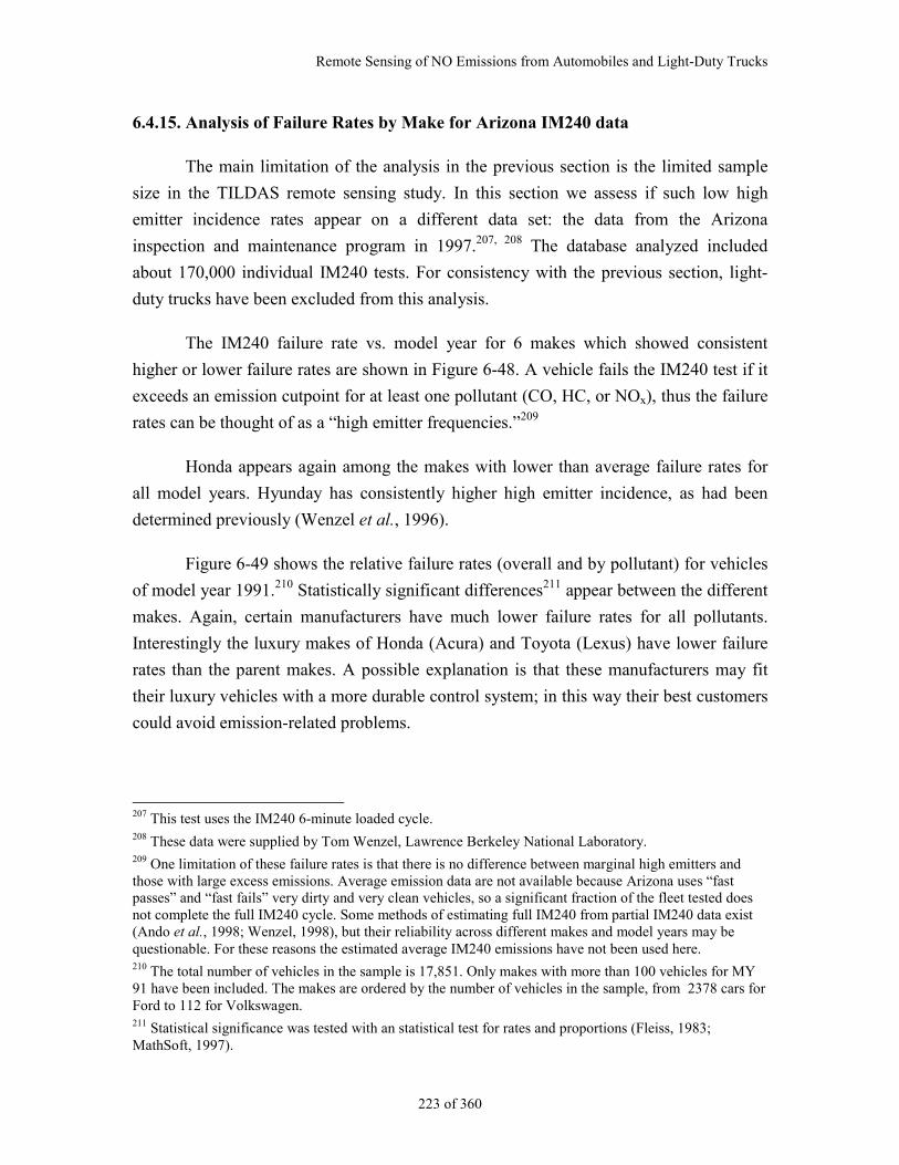
Remote Sensing of NO Emissions from Automobiles and Light-Duty Trucks

223 of 360

6.4.15. Analysis of Failure Rates by Make for Arizona IM240 data

The main limitation of the analysis in the previous section is the limited sample

size in the TILDAS remote sensing study. In this section we assess if such low high

emitter incidence rates appear on a different data set: the data from the Arizona

inspection and maintenance program in 1997.207, 208 The database analyzed included

about 170,000 individual IM240 tests. For consistency with the previous section, light-

duty trucks have been excluded from this analysis.

The IM240 failure rate vs. model year for 6 makes which showed consistent

higher or lower failure rates are shown in Figure 6-48. A vehicle fails the IM240 test if it

exceeds an emission cutpoint for at least one pollutant (CO, HC, or NOx), thus the failure

rates can be thought of as a “high emitter frequencies.”209

Honda appears again among the makes with lower than average failure rates for

all model years. Hyunday has consistently higher high emitter incidence, as had been

determined previously (Wenzel et al., 1996).

Figure 6-49 shows the relative failure rates (overall and by pollutant) for vehicles

of model year 1991.210 Statistically significant differences211 appear between the different

makes. Again, certain manufacturers have much lower failure rates for all pollutants.

Interestingly the luxury makes of Honda (Acura) and Toyota (Lexus) have lower failure

rates than the parent makes. A possible explanation is that these manufacturers may fit

their luxury vehicles with a more durable control system; in this way their best customers

could avoid emission-related problems.

207 This test uses the IM240 6-minute loaded cycle.208 These data were supplied by Tom Wenzel, Lawrence Berkeley National Laboratory.209 One limitation of these failure rates is that there is no difference between marginal high emitters andthose with large excess emissions. Average emission data are not available because Arizona uses “fastpasses” and “fast fails” very dirty and very clean vehicles, so a significant fraction of the fleet tested doesnot complete the full IM240 cycle. Some methods of estimating full IM240 from partial IM240 data exist(Ando et al., 1998; Wenzel, 1998), but their reliability across different makes and model years may bequestionable. For these reasons the estimated average IM240 emissions have not been used here.210 The total number of vehicles in the sample is 17,851. Only makes with more than 100 vehicles for MY91 have been included. The makes are ordered by the number of vehicles in the sample, from 2378 cars forFord to 112 for Volkswagen.211 Statistical significance was tested with an statistical test for rates and proportions (Fleiss, 1983;MathSoft, 1997).

Chapter 6

224 of 360

Another interesting feature of the IM240 data set is the fact that different makes

have significantly different failure rates for the different pollutants. For example,

Chrysler, Dodge, and Plymouth vehicles, the three of which are owned by Chrysler

Corporation, have significantly higher failure rates for NOx in 1991. Based on EPA

certification data, several Chrysler models of this model year did not use exhaust gas

recirculation (EGR) to reduce engine-out NOx emissions,212, 213 relying solely on the

three-way catalyst for NOx reduction. Such vehicles will likely fail for NO first when the

catalyst starts is deteriorated since their engine-out NOx emissions are about twice as high

as those of vehicles with EGR. Another manufacturer with high failure rates is Chevrolet

which is high for CO, indicating a tendency to run rich upon failure.

212 EGR can reduce engine-out NOx emissions levels by about a factor of 2-3 (see Figure 3-26).213 The Arizona data set did not include vehicle model, which precluded the verification of whether thefailing Chrysler models for NO were predominantly those without EGR.

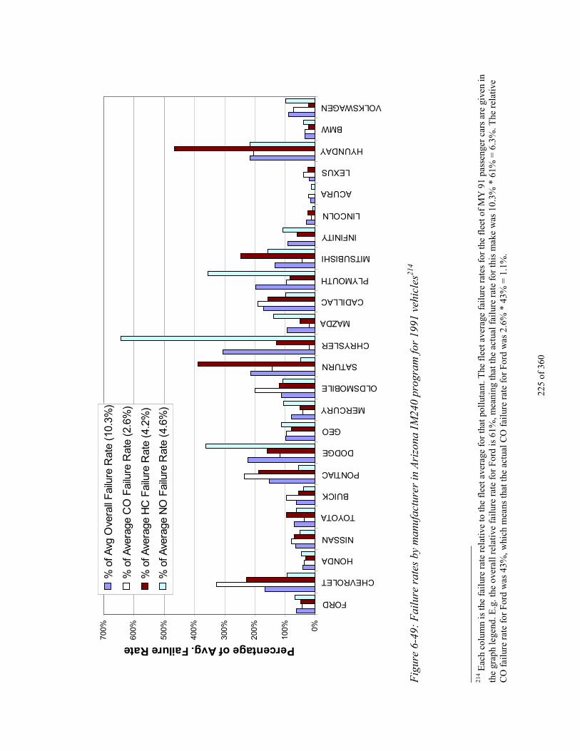
225

of 3

60

0%

100%

200%

300%

400%

500%

600%

700%

FORD

CHEVROLET

HONDA

NISSAN

TOYOTA

BUICK

PONTIAC

DODGE

GEO

MERCURY

OLDSMOBILE

SATURN

CHRYSLER

MAZDA

CADILLAC

PLYMOUTH

MITSUBISHI

INFINITY

LINCOLN

ACURA

LEXUS

HYUNDAY

BMW

VOLKSWAGEN

Percentage of Avg. Failure Rate%

of A

vg O

vera

ll F

ailu

re R

ate

(10.

3%)

% o

f Ave

rage

CO

Fai

lure

Rat

e (2

.6%

)

% o

f Ave

rage

HC

Fai

lure

Rat

e (4

.2%

)

% o

f Ave

rage

NO

Fai

lure

Rat

e (4

.6%

)

Fig

ure

6-49

: F

ailu

re r

ates

by

man

ufac

ture

r in

Ari

zona

IM

240

prog

ram

for

1991

veh

icle

s214

214 E

ach

colu

mn

is th

e fa

ilur

e ra

te r

elat

ive

to th

e fl

eet a

vera

ge f

or th

at p

ollu

tant

. The

fle

et a

vera

ge f

ailu

re r

ates

for

the

flee

t of

MY

91

pass

enge

r ca

rs a

re g

iven

inth

e gr

aph

lege

nd. E

.g. t

he o

vera

ll r

elat

ive

fail

ure

rate

for

For

d is

61%

, mea

ning

that

the

actu

al f

ailu

re r

ate

for

this

mak

e w

as 1

0.3%

* 6

1% =

6.3

%. T

he r

elat

ive

CO

fai

lure

rat

e fo

r F

ord

was

43%

, whi

ch m

eans

that

the

actu

al C

O f

ailu

re r

ate

for

For

d w

as 2

.6%

* 4

3% =

1.1

%.

Chapter 6

226 of 360

6.5. Conclusions of the NOx Remote Sensing Study

This study yielded a number of significant new findings with respect to the NO

emissions of on-road vehicles and the utility of remote sensing emissions measurements:

The TILDAS instrument consistently and accurately measured the NO emissions of

on-road vehicles. The NO emissions of low emitters were measured with precision of

approximately 5 ppm.

The measured vehicle fleet NO emissions closely fit a gamma distribution with the 10

percent of the fleet having the highest emissions contributing about 50 percent of the

total fleet emissions.

The NO emission factor in this study is about 80% of those measured in 3 recent

tunnel studies in California. The reason for this lower emission is not clear.

Newer vehicles have lower average NO emissions than older ones but high NO

emitters are found in every vehicle age cohort.

The light-duty trucks in this study are higher NO emitters than passenger cars. About

½ of the difference is due to their lower fuel economy while the other ½ reflects

higher NO exhaust concentrations, possibly due to more lenient emission standards.

The EMFAC emission model accurately predicts the NO emissions of recent model

years in our study and overpredicts those of older vehicles.

Analysis of the NO data with respect to the other simultaneously recorded data for the

subject vehicles shows that on a vehicle-by-vehicle basis NO emissions correlate only

weakly with vehicle specific power, speed, acceleration, CO emissions or HC

emissions.

High NO emitting vehicles cannot be identified by remote sensing of CO or HC

emissions and vice versa.

When these same data are aggregated into rank ordered population deciles, positive

correlations between decile averaged NO emissions and the decile averaged values of

vehicle specific power, CO, and HC for most of the vehicles appear.

Remote Sensing of NO Emissions from Automobiles and Light-Duty Trucks

227 of 360

When we compared the remotely sensed NO emissions measurements for 117

vehicles measured more than once, most of them were consistently low emitters.

About half of the high NO emitters were found to be consistently high while the other

half had significant variability.

The 10% highest emitters for each of CO, HC, and NO in this study constitute a

group of 23% of the vehicles with in excess of 60% of the emissions of each

pollutant.

Vehicles manufactured by Honda showed statistically significant lower NO emissions

than the rest of the fleet for model years 93-96. This was mostly due to the lack of

high emitters on the Honda fleet. Significant differences in high emitter incidence

among makes also appear in Arizona IM240 data.

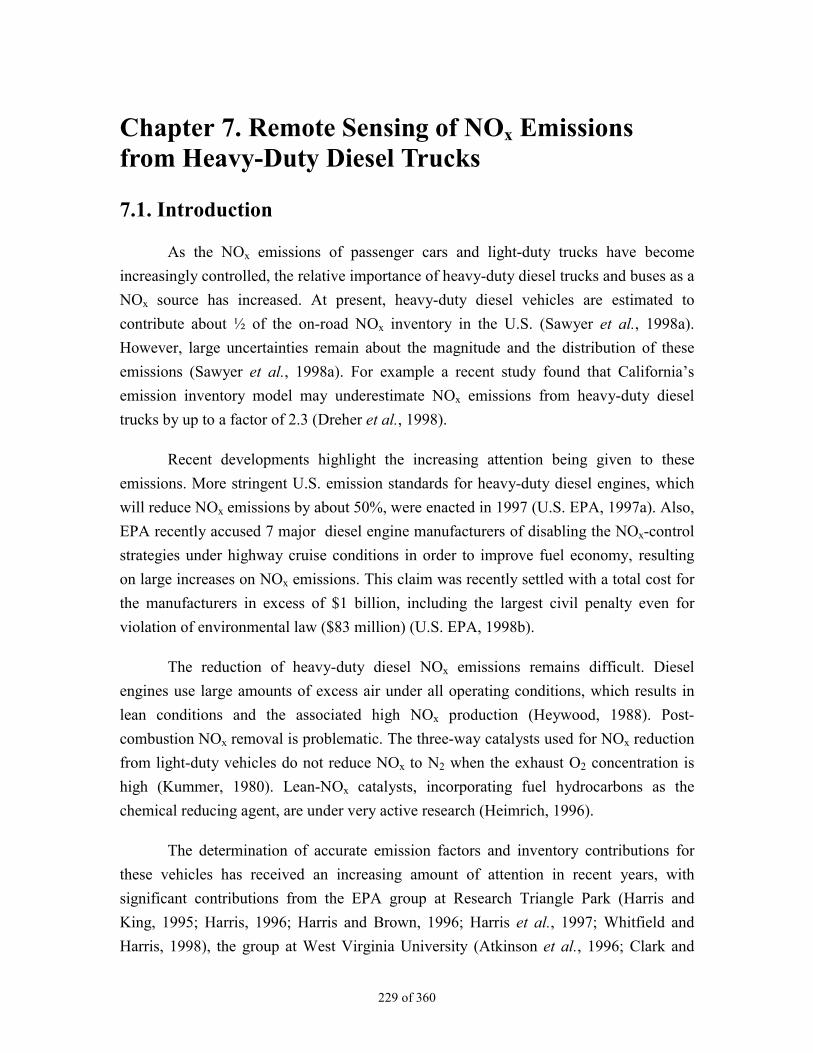
229 of 360

Chapter 7. Remote Sensing of NOx Emissionsfrom Heavy-Duty Diesel Trucks

7.1. Introduction

As the NOx emissions of passenger cars and light-duty trucks have become

increasingly controlled, the relative importance of heavy-duty diesel trucks and buses as a

NOx source has increased. At present, heavy-duty diesel vehicles are estimated to

contribute about ½ of the on-road NOx inventory in the U.S. (Sawyer et al., 1998a).

However, large uncertainties remain about the magnitude and the distribution of these

emissions (Sawyer et al., 1998a). For example a recent study found that California’s

emission inventory model may underestimate NOx emissions from heavy-duty diesel

trucks by up to a factor of 2.3 (Dreher et al., 1998).

Recent developments highlight the increasing attention being given to these

emissions. More stringent U.S. emission standards for heavy-duty diesel engines, which

will reduce NOx emissions by about 50%, were enacted in 1997 (U.S. EPA, 1997a). Also,

EPA recently accused 7 major diesel engine manufacturers of disabling the NOx-control

strategies under highway cruise conditions in order to improve fuel economy, resulting

on large increases on NOx emissions. This claim was recently settled with a total cost for

the manufacturers in excess of $1 billion, including the largest civil penalty even for

violation of environmental law ($83 million) (U.S. EPA, 1998b).

The reduction of heavy-duty diesel NOx emissions remains difficult. Diesel

engines use large amounts of excess air under all operating conditions, which results in

lean conditions and the associated high NOx production (Heywood, 1988). Post-

combustion NOx removal is problematic. The three-way catalysts used for NOx reduction

from light-duty vehicles do not reduce NOx to N2 when the exhaust O2 concentration is

high (Kummer, 1980). Lean-NOx catalysts, incorporating fuel hydrocarbons as the

chemical reducing agent, are under very active research (Heimrich, 1996).

The determination of accurate emission factors and inventory contributions for

these vehicles has received an increasing amount of attention in recent years, with

significant contributions from the EPA group at Research Triangle Park (Harris and

King, 1995; Harris, 1996; Harris and Brown, 1996; Harris et al., 1997; Whitfield and

Harris, 1998), the group at West Virginia University (Atkinson et al., 1996; Clark and

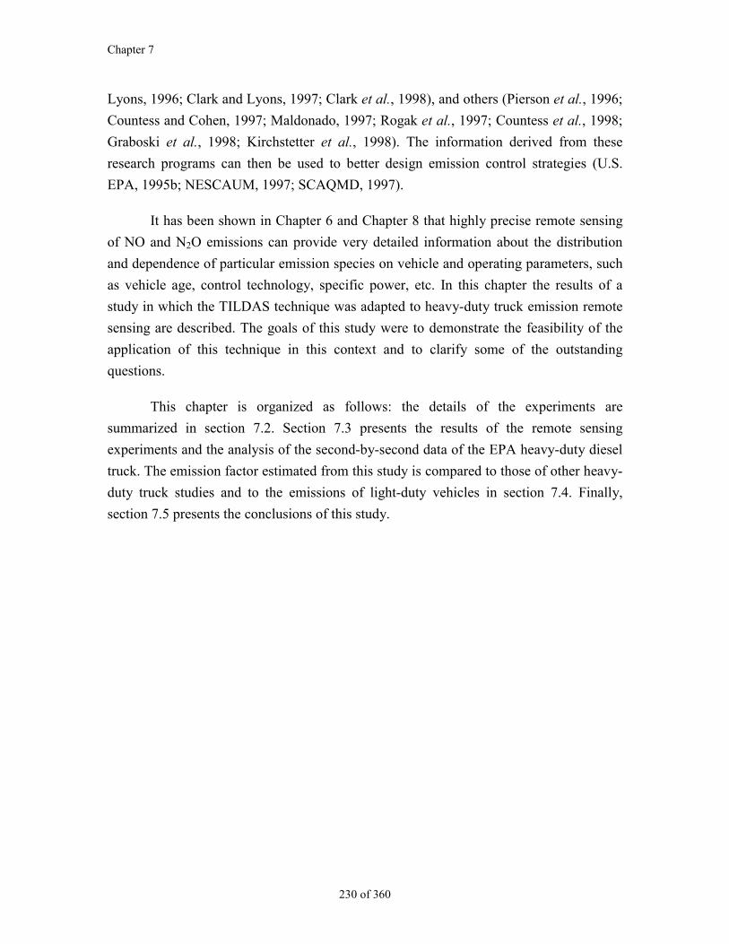
Chapter 7

230 of 360

Lyons, 1996; Clark and Lyons, 1997; Clark et al., 1998), and others (Pierson et al., 1996;

Countess and Cohen, 1997; Maldonado, 1997; Rogak et al., 1997; Countess et al., 1998;

Graboski et al., 1998; Kirchstetter et al., 1998). The information derived from these

research programs can then be used to better design emission control strategies (U.S.

EPA, 1995b; NESCAUM, 1997; SCAQMD, 1997).

It has been shown in Chapter 6 and Chapter 8 that highly precise remote sensing

of NO and N2O emissions can provide very detailed information about the distribution

and dependence of particular emission species on vehicle and operating parameters, such

as vehicle age, control technology, specific power, etc. In this chapter the results of a

study in which the TILDAS technique was adapted to heavy-duty truck emission remote

sensing are described. The goals of this study were to demonstrate the feasibility of the

application of this technique in this context and to clarify some of the outstanding

questions.

This chapter is organized as follows: the details of the experiments are

summarized in section 7.2. Section 7.3 presents the results of the remote sensing

experiments and the analysis of the second-by-second data of the EPA heavy-duty diesel

truck. The emission factor estimated from this study is compared to those of other heavy-

duty truck studies and to the emissions of light-duty vehicles in section 7.4. Finally,

section 7.5 presents the conclusions of this study.

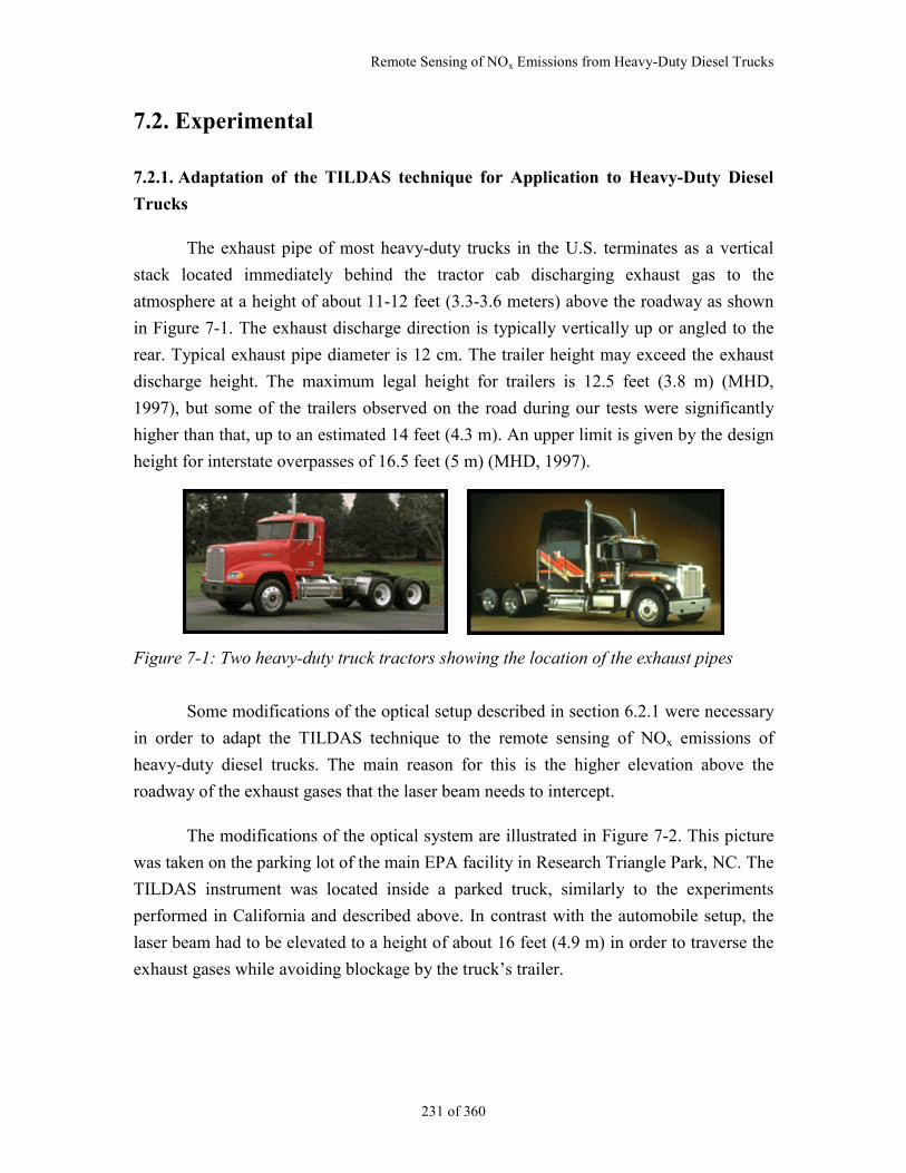
Remote Sensing of NOx Emissions from Heavy-Duty Diesel Trucks

231 of 360

7.2. Experimental

7.2.1. Adaptation of the TILDAS technique for Application to Heavy-Duty Diesel

Trucks

The exhaust pipe of most heavy-duty trucks in the U.S. terminates as a vertical

stack located immediately behind the tractor cab discharging exhaust gas to the

atmosphere at a height of about 11-12 feet (3.3-3.6 meters) above the roadway as shown

in Figure 7-1. The exhaust discharge direction is typically vertically up or angled to the

rear. Typical exhaust pipe diameter is 12 cm. The trailer height may exceed the exhaust

discharge height. The maximum legal height for trailers is 12.5 feet (3.8 m) (MHD,

1997), but some of the trailers observed on the road during our tests were significantly

higher than that, up to an estimated 14 feet (4.3 m). An upper limit is given by the design

height for interstate overpasses of 16.5 feet (5 m) (MHD, 1997).

Figure 7-1: Two heavy-duty truck tractors showing the location of the exhaust pipes

Some modifications of the optical setup described in section 6.2.1 were necessary

in order to adapt the TILDAS technique to the remote sensing of NOx emissions of

heavy-duty diesel trucks. The main reason for this is the higher elevation above the

roadway of the exhaust gases that the laser beam needs to intercept.

The modifications of the optical system are illustrated in Figure 7-2. This picture

was taken on the parking lot of the main EPA facility in Research Triangle Park, NC. The

TILDAS instrument was located inside a parked truck, similarly to the experiments

performed in California and described above. In contrast with the automobile setup, the

laser beam had to be elevated to a height of about 16 feet (4.9 m) in order to traverse the

exhaust gases while avoiding blockage by the truck’s trailer.

Chapter 7

232 of 360

RetroReflector

TILDASInstrument

EPA’sInstrumented

Truck2nd TurningMirror

1st TurningMirror

Figure 7-2: Optical layout for the remote sensing of emissions from heavy-duty dieseltrucks

To accomplish that objective the laser beam was first sent to a tripod-mounted

turning mirror located about 4 feet (1.2 m) above the ground. This mirror directed the

beam to a second tripod-mounted mirror which was fixed to the top of the instrument

truck. The center of this mirror was located at a height of about 14 feet (4.3 m). From

there the laser beam path passed over the road to the retroreflector, which was mounted

also at 14 feet on a large tripod and stabilized with the help of 9 guide wires. The laser

beam then returned to the optical table following the same path. The total optical

pathlength of the laser beam in this configuration was about 165 feet (50m).

The alignment of the system was performed with the help of the visible HeNe

laser as described for the automotive experiments. The telescope objective available in

the laser optical table was used to position the outgoing beam in the retroreflector.

The triggering of the data acquisition function also needed a modification from

the automobile study configuration. In this case, the laser beam is not interrupted by the

vehicle and thus the detector signal does not provide an indication for the start of the data

acquisition. The solution chosen was to use manual triggering the data acquisition

function from the system’s computer keyboard when the truck was about to pass under

the laser path.215

215 A more sophisticated approach could be used in future studies to provide automatic triggering operation.A visible HeNe laser could be sent across the road to a second retro-reflector and its signal monitored by anadditional detector. This beam would be set at a height above all automobiles and light-duty trucks but

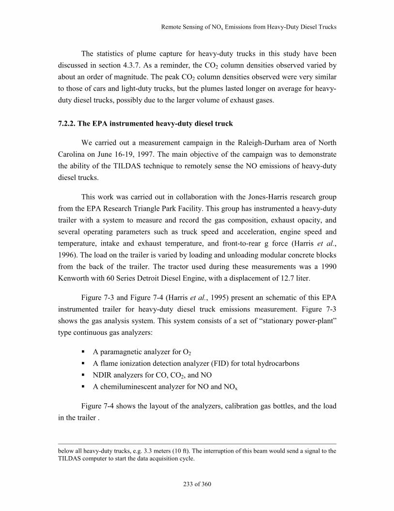
Remote Sensing of NOx Emissions from Heavy-Duty Diesel Trucks

233 of 360

The statistics of plume capture for heavy-duty trucks in this study have been

discussed in section 4.3.7. As a reminder, the CO2 column densities observed varied by

about an order of magnitude. The peak CO2 column densities observed were very similar

to those of cars and light-duty trucks, but the plumes lasted longer on average for heavy-

duty diesel trucks, possibly due to the larger volume of exhaust gases.

7.2.2. The EPA instrumented heavy-duty diesel truck

We carried out a measurement campaign in the Raleigh-Durham area of North

Carolina on June 16-19, 1997. The main objective of the campaign was to demonstrate

the ability of the TILDAS technique to remotely sense the NO emissions of heavy-duty

diesel trucks.

This work was carried out in collaboration with the Jones-Harris research group

from the EPA Research Triangle Park Facility. This group has instrumented a heavy-duty

trailer with a system to measure and record the gas composition, exhaust opacity, and

several operating parameters such as truck speed and acceleration, engine speed and

temperature, intake and exhaust temperature, and front-to-rear g force (Harris et al.,

1996). The load on the trailer is varied by loading and unloading modular concrete blocks

from the back of the trailer. The tractor used during these measurements was a 1990

Kenworth with 60 Series Detroit Diesel Engine, with a displacement of 12.7 liter.

Figure 7-3 and Figure 7-4 (Harris et al., 1995) present an schematic of this EPA

instrumented trailer for heavy-duty diesel truck emissions measurement. Figure 7-3

shows the gas analysis system. This system consists of a set of “stationary power-plant”

type continuous gas analyzers:

A paramagnetic analyzer for O2

A flame ionization detection analyzer (FID) for total hydrocarbons

NDIR analyzers for CO, CO2, and NO

A chemiluminescent analyzer for NO and NOx

Figure 7-4 shows the layout of the analyzers, calibration gas bottles, and the load

in the trailer .

below all heavy-duty trucks, e.g. 3.3 meters (10 ft). The interruption of this beam would send a signal to theTILDAS computer to start the data acquisition cycle.

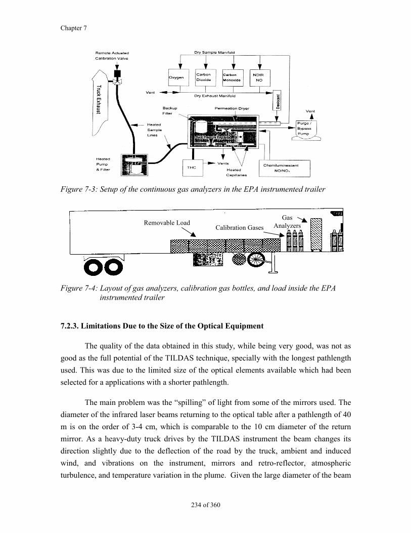
Chapter 7

234 of 360

Figure 7-3: Setup of the continuous gas analyzers in the EPA instrumented trailer

Removable LoadCalibration Gases

GasAnalyzers

Figure 7-4: Layout of gas analyzers, calibration gas bottles, and load inside the EPAinstrumented trailer

7.2.3. Limitations Due to the Size of the Optical Equipment

The quality of the data obtained in this study, while being very good, was not as

good as the full potential of the TILDAS technique, specially with the longest pathlength

used. This was due to the limited size of the optical elements available which had been

selected for a applications with a shorter pathlength.

The main problem was the “spilling” of light from some of the mirrors used. The

diameter of the infrared laser beams returning to the optical table after a pathlength of 40

m is on the order of 3-4 cm, which is comparable to the 10 cm diameter of the return

mirror. As a heavy-duty truck drives by the TILDAS instrument the beam changes its

direction slightly due to the deflection of the road by the truck, ambient and induced

wind, and vibrations on the instrument, mirrors and retro-reflector, atmospheric

turbulence, and temperature variation in the plume. Given the large diameter of the beam

Remote Sensing of NOx Emissions from Heavy-Duty Diesel Trucks

235 of 360

relative to the return mirror, some of the returning light did not hit the mirror and was

lost. This caused loss of some signal intensity, and also caused a large amplification in

optical fringes in some of the passes. This problem can be eliminated from future studies

by using larger optics for the key elements.

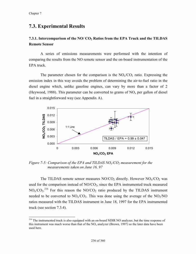
Chapter 7

236 of 360

7.3. Experimental Results

7.3.1. Intercomparison of the NO/ CO2 Ratios from the EPA Truck and the TILDAS

Remote Sensor

A series of emissions measurements were performed with the intention of

comparing the results from the NO remote sensor and the on-board instrumentation of the

EPA truck.

The parameter chosen for the comparison is the NOx/CO2 ratio. Expressing the

emission index in this way avoids the problem of determining the air-to-fuel ratio in the

diesel engine which, unlike gasoline engines, can vary by more than a factor of 2

(Heywood, 1988). This parameter can be converted to grams of NOx per gallon of diesel

fuel in a straightforward way (see Appendix A).

0.000

0.003

0.006

0.009

0.012

0.015

0 0.003 0.006 0.009 0.012 0.015

NOx/CO2 EPA

NO

x/C

O2

TIL

DA

S

1:1 Line

TILDAS / EPA = 0.99 ± 0.047

Figure 7-5: Comparison of the EPA and TILDAS NOx/CO2 measurement for themeasurements taken on June 16, 97

The TILDAS remote sensor measures NO/CO2 directly. However NOx/CO2 was

used for the comparison instead of NO/CO2, since the EPA instrumented truck measured

NOx/CO2.216 For this reason the NO/CO2 ratio produced by the TILDAS instrument

needed to be converted to NOx/CO2. This was done using the average of the NO2/NO

ratios measured with the TILDAS instrument in June 18, 1997 for the EPA instrumented

truck (see section 7.3.4).

216 The instrumented truck is also equipped with an on-board NDIR NO analyzer, but the time response ofthis instrument was much worse than that of the NOx analyzer (Brown, 1997) so the later data have beenused here.

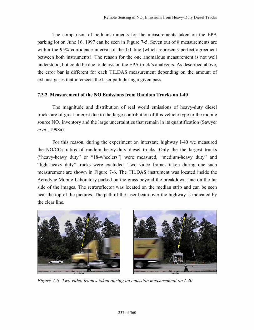
Remote Sensing of NOx Emissions from Heavy-Duty Diesel Trucks

237 of 360

The comparison of both instruments for the measurements taken on the EPA

parking lot on June 16, 1997 can be seen in Figure 7-5. Seven out of 8 measurements are

within the 95% confidence interval of the 1:1 line (which represents perfect agreement

between both instruments). The reason for the one anomalous measurement is not well

understood, but could be due to delays on the EPA truck’s analyzers. As described above,

the error bar is different for each TILDAS measurement depending on the amount of

exhaust gases that intersects the laser path during a given pass.

7.3.2. Measurement of the NO Emissions from Random Trucks on I-40

The magnitude and distribution of real world emissions of heavy-duty diesel

trucks are of great interest due to the large contribution of this vehicle type to the mobile

source NOx inventory and the large uncertainties that remain in its quantification (Sawyer

et al., 1998a).

For this reason, during the experiment on interstate highway I-40 we measured

the NO/CO2 ratios of random heavy-duty diesel trucks. Only the the largest trucks

(“heavy-heavy duty” or “18-wheelers”) were measured, “medium-heavy duty” and

“light-heavy duty” trucks were excluded. Two video frames taken during one such

measurement are shown in Figure 7-6. The TILDAS instrument was located inside the

Aerodyne Mobile Laboratory parked on the grass beyond the breakdown lane on the far

side of the images. The retroreflector was located on the median strip and can be seen

near the top of the pictures. The path of the laser beam over the highway is indicated by

the clear line.

Figure 7-6: Two video frames taken during an emission measurement on I-40

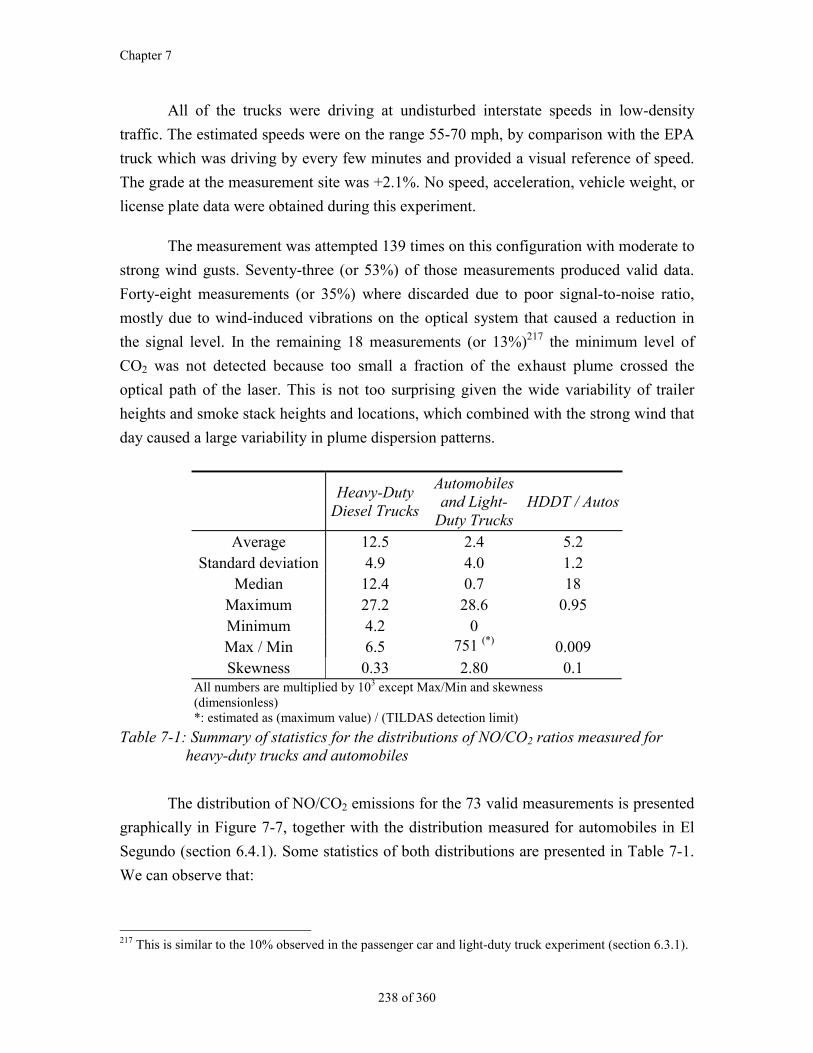
Chapter 7

238 of 360

All of the trucks were driving at undisturbed interstate speeds in low-density

traffic. The estimated speeds were on the range 55-70 mph, by comparison with the EPA

truck which was driving by every few minutes and provided a visual reference of speed.

The grade at the measurement site was +2.1%. No speed, acceleration, vehicle weight, or

license plate data were obtained during this experiment.

The measurement was attempted 139 times on this configuration with moderate to

strong wind gusts. Seventy-three (or 53%) of those measurements produced valid data.

Forty-eight measurements (or 35%) where discarded due to poor signal-to-noise ratio,

mostly due to wind-induced vibrations on the optical system that caused a reduction in

the signal level. In the remaining 18 measurements (or 13%)217 the minimum level of

CO2 was not detected because too small a fraction of the exhaust plume crossed the

optical path of the laser. This is not too surprising given the wide variability of trailer

heights and smoke stack heights and locations, which combined with the strong wind that

day caused a large variability in plume dispersion patterns.

Heavy-DutyDiesel Trucks

Automobilesand Light-

Duty TrucksHDDT / Autos

Average 12.5 2.4 5.2Standard deviation 4.9 4.0 1.2

Median 12.4 0.7 18Maximum 27.2 28.6 0.95Minimum 4.2 0Max / Min 6.5 751 (*) 0.009Skewness 0.33 2.80 0.1

All numbers are multiplied by 103 except Max/Min and skewness(dimensionless)*: estimated as (maximum value) / (TILDAS detection limit)

Table 7-1: Summary of statistics for the distributions of NO/CO2 ratios measured forheavy-duty trucks and automobiles

The distribution of NO/CO2 emissions for the 73 valid measurements is presented

graphically in Figure 7-7, together with the distribution measured for automobiles in El

Segundo (section 6.4.1). Some statistics of both distributions are presented in Table 7-1.

We can observe that:

217 This is similar to the 10% observed in the passenger car and light-duty truck experiment (section 6.3.1).

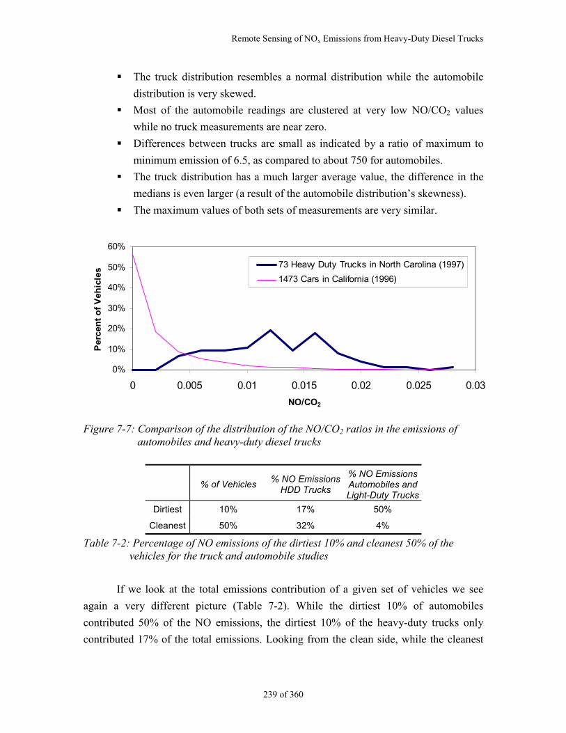
Remote Sensing of NOx Emissions from Heavy-Duty Diesel Trucks

239 of 360

The truck distribution resembles a normal distribution while the automobile

distribution is very skewed.

Most of the automobile readings are clustered at very low NO/CO2 values

while no truck measurements are near zero.

Differences between trucks are small as indicated by a ratio of maximum to

minimum emission of 6.5, as compared to about 750 for automobiles.

The truck distribution has a much larger average value, the difference in the

medians is even larger (a result of the automobile distribution’s skewness).

The maximum values of both sets of measurements are very similar.

0%

10%

20%

30%

40%

50%

60%

0 0.005 0.01 0.015 0.02 0.025 0.03

NO/CO2

Per

cen

t o

f V

ehic

les

73 Heavy Duty Trucks in North Carolina (1997)

1473 Cars in California (1996)

Figure 7-7: Comparison of the distribution of the NO/CO2 ratios in the emissions ofautomobiles and heavy-duty diesel trucks

% of Vehicles% NO Emissions

HDD Trucks

% NO EmissionsAutomobiles andLight-Duty Trucks

Dirtiest 10% 17% 50%

Cleanest 50% 32% 4%

Table 7-2: Percentage of NO emissions of the dirtiest 10% and cleanest 50% of thevehicles for the truck and automobile studies

If we look at the total emissions contribution of a given set of vehicles we see

again a very different picture (Table 7-2). While the dirtiest 10% of automobiles

contributed 50% of the NO emissions, the dirtiest 10% of the heavy-duty trucks only

contributed 17% of the total emissions. Looking from the clean side, while the cleanest

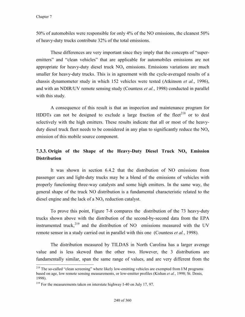
Chapter 7

240 of 360

50% of automobiles were responsible for only 4% of the NO emissions, the cleanest 50%

of heavy-duty trucks contribute 32% of the total emissions.

These differences are very important since they imply that the concepts of “super-

emitters” and “clean vehicles” that are applicable for automobiles emissions are not

appropriate for heavy-duty diesel truck NOx emissions. Emissions variations are much

smaller for heavy-duty trucks. This is in agreement with the cycle-averaged results of a

chassis dynamometer study in which 152 vehicles were tested (Atkinson et al., 1996),

and with an NDIR/UV remote sensing study (Countess et al., 1998) conducted in parallel

with this study.

A consequence of this result is that an inspection and maintenance program for

HDDTs can not be designed to exclude a large fraction of the fleet218 or to deal

selectively with the high emitters. These results indicate that all or most of the heavy-

duty diesel truck fleet needs to be considered in any plan to significantly reduce the NOx

emission of this mobile source component.

7.3.3. Origin of the Shape of the Heavy-Duty Diesel Truck NOx Emission

Distribution

It was shown in section 6.4.2 that the distribution of NO emissions from

passenger cars and light-duty trucks may be a blend of the emissions of vehicles with

properly functioning three-way catalysts and some high emitters. In the same way, the

general shape of the truck NO distribution is a fundamental characteristic related to the

diesel engine and the lack of a NOx reduction catalyst.

To prove this point, Figure 7-8 compares the distribution of the 73 heavy-duty

trucks shown above with the distribution of the second-by-second data from the EPA

instrumented truck,219 and the distribution of NO emissions measured with the UV

remote sensor in a study carried out in parallel with this one (Countess et al., 1998).

The distribution measured by TILDAS in North Carolina has a larger average

value and is less skewed than the other two. However, the 3 distributions are

fundamentally similar, span the same range of values, and are very different from the 218 The so-called “clean screening” where likely low-emitting vehicles are exempted from I/M programsbased on age, low remote sensing measurements, or low-emitter profiles (Kishan et al., 1998; St. Denis,1998).219 For the measurements taken on interstate highway I-40 on July 17, 97.

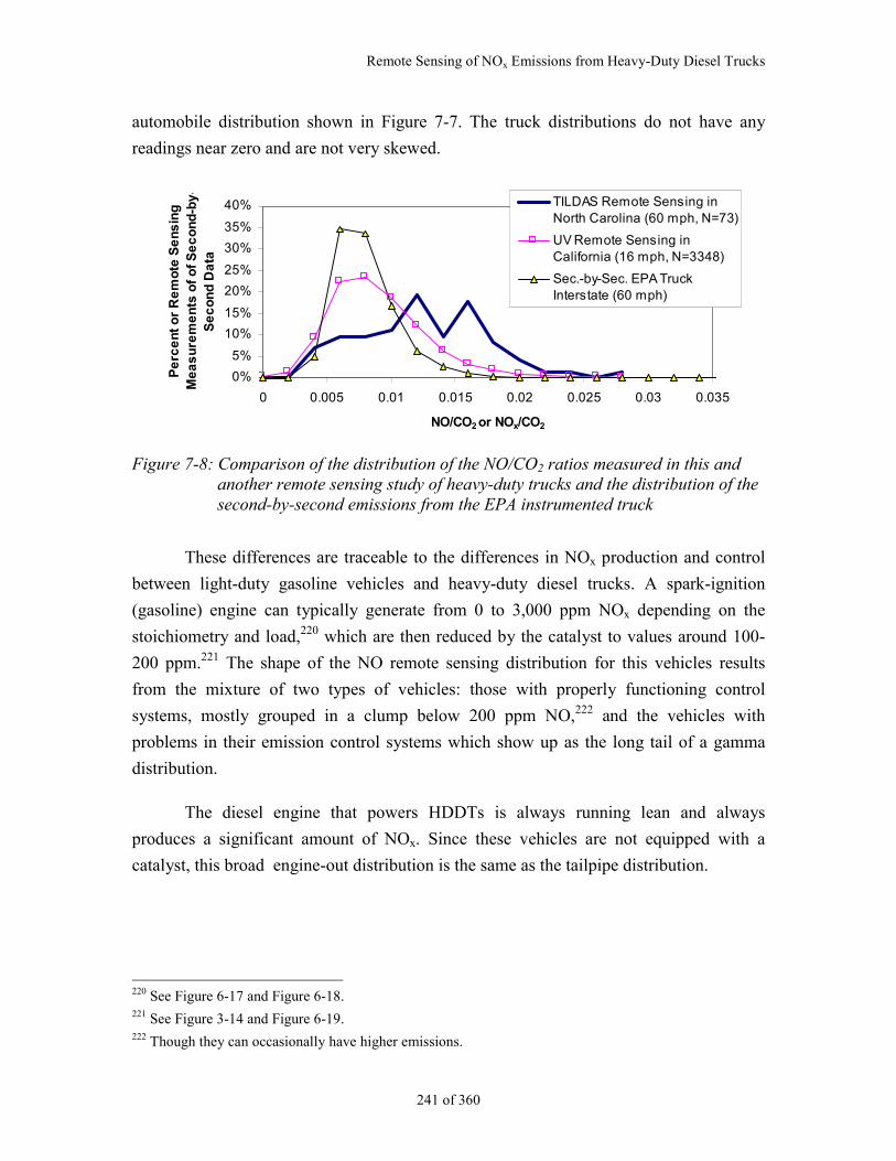
Remote Sensing of NOx Emissions from Heavy-Duty Diesel Trucks

241 of 360

automobile distribution shown in Figure 7-7. The truck distributions do not have any

readings near zero and are not very skewed.

0%

5%

10%

15%

20%

25%

30%

35%

40%

0 0.005 0.01 0.015 0.02 0.025 0.03 0.035

NO/CO2 or NOx/CO2

Pe

rce

nt

or

Re

mo

te S

en

sin

g

Me

as

ure

me

nts

of

of

Se

co

nd

-by

-S

ec

on

d D

ata

TILDAS Remote Sensing inNorth Carolina (60 mph, N=73)

UV Remote Sensing inCalifornia (16 mph, N=3348)

Sec.-by-Sec. EPA TruckInterstate (60 mph)

Figure 7-8: Comparison of the distribution of the NO/CO2 ratios measured in this andanother remote sensing study of heavy-duty trucks and the distribution of thesecond-by-second emissions from the EPA instrumented truck

These differences are traceable to the differences in NOx production and control

between light-duty gasoline vehicles and heavy-duty diesel trucks. A spark-ignition

(gasoline) engine can typically generate from 0 to 3,000 ppm NOx depending on the

stoichiometry and load,220 which are then reduced by the catalyst to values around 100-

200 ppm.221 The shape of the NO remote sensing distribution for this vehicles results

from the mixture of two types of vehicles: those with properly functioning control

systems, mostly grouped in a clump below 200 ppm NO,222 and the vehicles with

problems in their emission control systems which show up as the long tail of a gamma

distribution.

The diesel engine that powers HDDTs is always running lean and always

produces a significant amount of NOx. Since these vehicles are not equipped with a

catalyst, this broad engine-out distribution is the same as the tailpipe distribution.

220 See Figure 6-17 and Figure 6-18.221 See Figure 3-14 and Figure 6-19.222 Though they can occasionally have higher emissions.

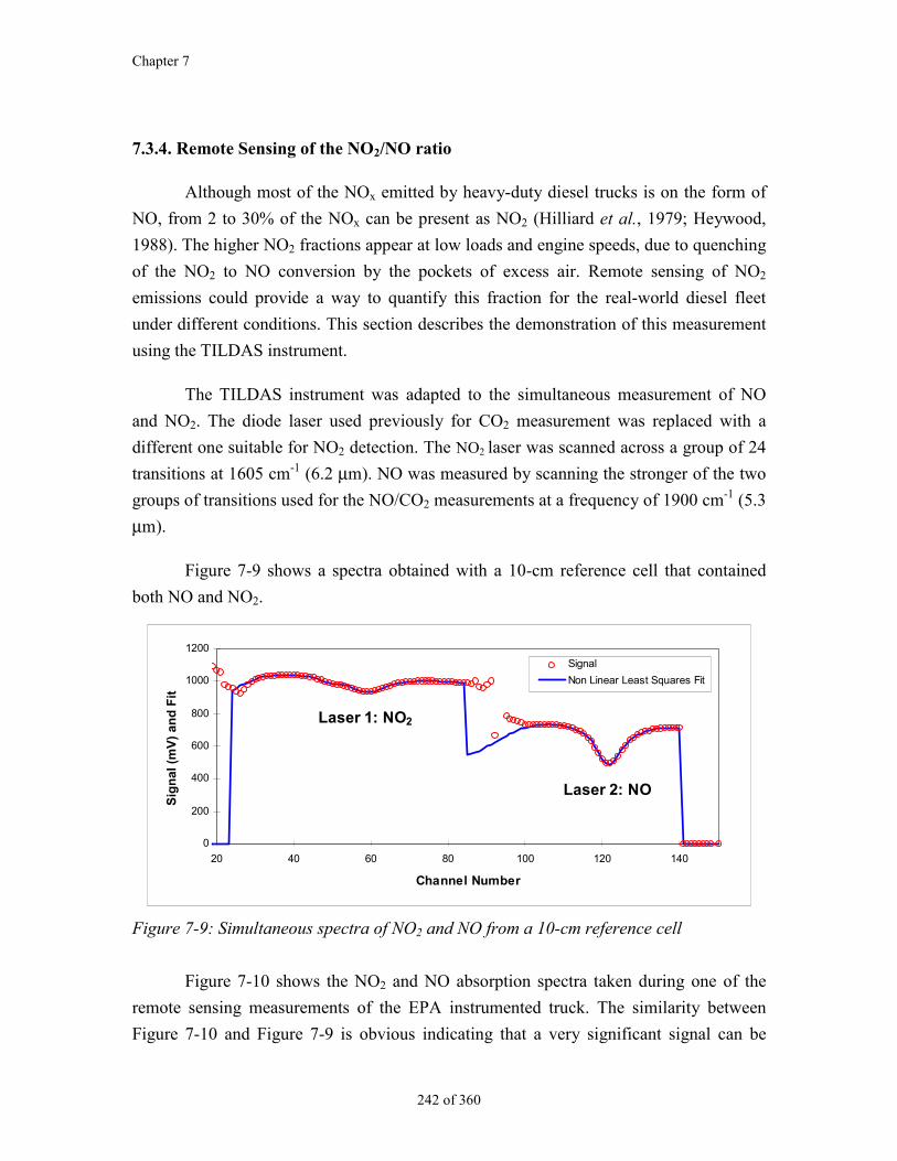
Chapter 7

242 of 360

7.3.4. Remote Sensing of the NO2/NO ratio

Although most of the NOx emitted by heavy-duty diesel trucks is on the form of

NO, from 2 to 30% of the NOx can be present as NO2 (Hilliard et al., 1979; Heywood,

1988). The higher NO2 fractions appear at low loads and engine speeds, due to quenching

of the NO2 to NO conversion by the pockets of excess air. Remote sensing of NO2

emissions could provide a way to quantify this fraction for the real-world diesel fleet

under different conditions. This section describes the demonstration of this measurement

using the TILDAS instrument.

The TILDAS instrument was adapted to the simultaneous measurement of NO

and NO2. The diode laser used previously for CO2 measurement was replaced with a

different one suitable for NO2 detection. The NO2 laser was scanned across a group of 24

transitions at 1605 cm-1 (6.2 µm). NO was measured by scanning the stronger of the two

groups of transitions used for the NO/CO2 measurements at a frequency of 1900 cm-1 (5.3

µm).

Figure 7-9 shows a spectra obtained with a 10-cm reference cell that contained

both NO and NO2.

0

200

400

600

800

1000

1200

20 40 60 80 100 120 140

Channel Number

Sig

nal

(m

V)

and

Fit

Signal

Non Linear Least Squares Fit

Laser 1: NO2

Laser 2: NO

Figure 7-9: Simultaneous spectra of NO2 and NO from a 10-cm reference cell

Figure 7-10 shows the NO2 and NO absorption spectra taken during one of the

remote sensing measurements of the EPA instrumented truck. The similarity between

Figure 7-10 and Figure 7-9 is obvious indicating that a very significant signal can be

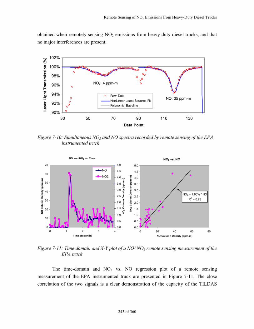
Remote Sensing of NOx Emissions from Heavy-Duty Diesel Trucks

243 of 360

obtained when remotely sensing NO2 emissions from heavy-duty diesel trucks, and that

no major interferences are present.

90%

92%

94%

96%

98%

100%

102%

30 50 70 90 110 130

Data Point

Las

er L

igh

t T

ran

smis

sio

n (

%)

Raw Data

NonLinear Least Squares Fit

Polynomial Baseline

NO2: 4 ppm-m

NO: 35 ppm-m

Figure 7-10: Simultaneous NO2 and NO spectra recorded by remote sensing of the EPAinstrumented truck

NO and NO2 vs. Time

0

10

20

30

40

50

60

70

0 1 2 3 4

Time (seconds)

NO

Co

lum

n D

ensi

ty (

pp

m-m

)

0.0

0.5

1.0

1.5

2.0

2.5

3.0

3.5

4.0

4.5

5.0

NO

2 C

olu

mn

Den

sity

(p

pm

-m)

NO

NO2

NO2 vs. NO

NO2 = 7.96% * NO

R2 = 0.78

0.0

0.5

1.0

1.5

2.0

2.5

3.0

3.5

4.0

4.5

5.0

0 20 40 60 80

NO Column Density (ppm-m)

NO

2 C

olu

mn

Den

sity

(p

pm

-m)

Figure 7-11: Time domain and X-Y plot of a NO/ NO2 remote sensing measurement of theEPA truck

The time-domain and NO2 vs. NO regression plot of a remote sensing

measurement of the EPA instrumented truck are presented in Figure 7-11. The close

correlation of the two signals is a clear demonstration of the capacity of the TILDAS

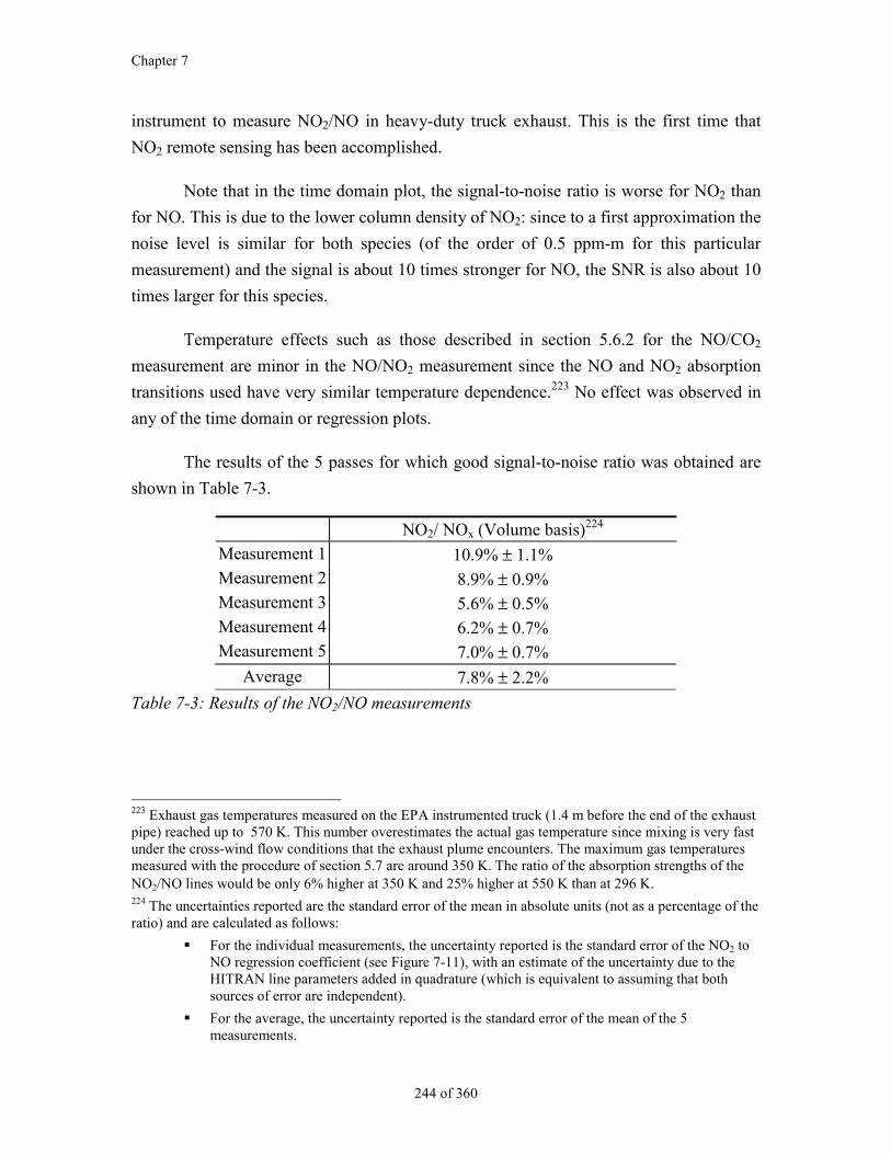
Chapter 7

244 of 360

instrument to measure NO2/NO in heavy-duty truck exhaust. This is the first time that

NO2 remote sensing has been accomplished.

Note that in the time domain plot, the signal-to-noise ratio is worse for NO2 than

for NO. This is due to the lower column density of NO2: since to a first approximation the

noise level is similar for both species (of the order of 0.5 ppm-m for this particular

measurement) and the signal is about 10 times stronger for NO, the SNR is also about 10

times larger for this species.

Temperature effects such as those described in section 5.6.2 for the NO/CO2

measurement are minor in the NO/NO2 measurement since the NO and NO2 absorption

transitions used have very similar temperature dependence.223 No effect was observed in

any of the time domain or regression plots.

The results of the 5 passes for which good signal-to-noise ratio was obtained are

shown in Table 7-3.

NO2/ NOx (Volume basis)224

Measurement 1 10.9% ± 1.1%Measurement 2 8.9% ± 0.9%Measurement 3 5.6% ± 0.5%Measurement 4 6.2% ± 0.7%Measurement 5 7.0% ± 0.7%

Average 7.8% ± 2.2%

Table 7-3: Results of the NO2/NO measurements

223 Exhaust gas temperatures measured on the EPA instrumented truck (1.4 m before the end of the exhaustpipe) reached up to 570 K. This number overestimates the actual gas temperature since mixing is very fastunder the cross-wind flow conditions that the exhaust plume encounters. The maximum gas temperaturesmeasured with the procedure of section 5.7 are around 350 K. The ratio of the absorption strengths of theNO2/NO lines would be only 6% higher at 350 K and 25% higher at 550 K than at 296 K.224 The uncertainties reported are the standard error of the mean in absolute units (not as a percentage of theratio) and are calculated as follows:

For the individual measurements, the uncertainty reported is the standard error of the NO2 toNO regression coefficient (see Figure 7-11), with an estimate of the uncertainty due to theHITRAN line parameters added in quadrature (which is equivalent to assuming that bothsources of error are independent).

For the average, the uncertainty reported is the standard error of the mean of the 5measurements.

Remote Sensing of NOx Emissions from Heavy-Duty Diesel Trucks

245 of 360

The measured NO2/NOx ratios range from 5.6% to 10.9% by volume. The average

ratio for the 5 measurements was 7.8% ± 2.2%. No comparison can be made with the on-

board instrumentation of the EPA truck in this case since the on-board system is not

designed or built for NO2 quantification (Brown, 1997).225

These results are within the ranges of those reported in the literature. Hilliard and

Wheeler (Hilliard 1979) reported that 2% to 30% (on a volume basis) of the total NOx

emitted from a diesel engine could be in the form of NO2. They found that this ratio was

higher under light load and low engine speed conditions and lower at high load and high

engine speeds.

Harris et al. (Harris et al., 1987) measured NO2 concentration in the range of 0.4

to 33 ppmv of the exhaust with a low-pressure sampling TILDAS system, but did not

report NO2/NOx ratios. They do report higher NO2 concentrations at low loads, in

agreement with the results of Hilliard and Wheeler.

Clark et al. (Clark et al., 1998) recently reported the results of a study in which

diesel engines were operated in steady state conditions on a chassis dynamometer yielded

ratios in the 2.2%-18% range. The authors also reported some results from testing diesel

buses on an engine dynamometer on the Central Business District cycle. Ratios of up to

4% were measured from current engines under those conditions. The trends with speed

and load were consistent with those of Hilliard.

The 5-11% range that we measured with the TILDAS instrument while the EPA

instrumented truck was run at about 20 mph under mild accelerations are consistent with

these literature studies.

7.3.5. Opacity Measurement

Particulate air pollution has attracted a great deal of interest in recent years due to

the recently discovered health effects associated with high environmental concentrations

225 Although the system is equipped with two chemiluminescent NO/NOx instruments, they aremanufactured by different companies and have fundamentally different sample delivery systems. Whileone of the instrument is used as an NO analyzer (Thermo Electron) and the other one as an NOx analyzer(Horiba), the response of the two instruments is very different. The NOx instrument peaks and troughs aremuch sharper than the NO instrument, possibly because of some flow capillary irregularities in the NOinstrument (Brown, 1997). This invalidates the subtraction method of NO2 quantification. An attempt tonumerically convolve the response of the faster instrument with the response function of the slowerinstrument proved unsuccessful in producing a credible NO2 vs. time signal.

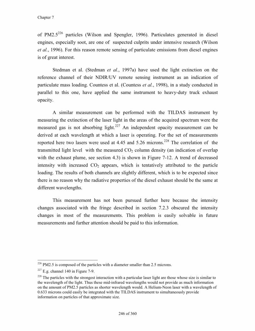
Chapter 7

246 of 360

of PM2.5226 particles (Wilson and Spengler, 1996). Particulates generated in diesel

engines, especially soot, are one of suspected culprits under intensive research (Wilson

et al., 1996). For this reason remote sensing of particulate emissions from diesel engines

is of great interest.

Stedman et al. (Stedman et al., 1997a) have used the light extinction on the

reference channel of their NDIR/UV remote sensing instrument as an indication of

particulate mass loading. Countess et al. (Countess et al., 1998), in a study conducted in

parallel to this one, have applied the same instrument to heavy-duty truck exhaust

opacity.

A similar measurement can be performed with the TILDAS instrument by

measuring the extinction of the laser light in the areas of the acquired spectrum were the

measured gas is not absorbing light.227 An independent opacity measurement can be

derived at each wavelength at which a laser is operating. For the set of measurements

reported here two lasers were used at 4.45 and 5.26 microns.228 The correlation of the

transmitted light level with the measured CO2 column density (an indication of overlap

with the exhaust plume, see section 4.3) is shown in Figure 7-12. A trend of decreased

intensity with increased CO2 appears, which is tentatively attributed to the particle

loading. The results of both channels are slightly different, which is to be expected since

there is no reason why the radiative properties of the diesel exhaust should be the same at

different wavelengths.

This measurement has not been pursued further here because the intensity

changes associated with the fringe described in section 7.2.3 obscured the intensity

changes in most of the measurements. This problem is easily solvable in future

measurements and further attention should be paid to this information.

226 PM2.5 is composed of the particles with a diameter smaller than 2.5 microns.227 E.g. channel 140 in Figure 7-9.228 The particles with the strongest interaction with a particular laser light are those whose size is similar tothe wavelength of the light. Thus these mid-infrared wavelengths would not provide as much informationon the amount of PM2.5 particles as shorter wavelength would. A Helium-Neon laser with a wavelength of0.633 microns could easily be integrated with the TILDAS instrument to simultaneously provideinformation on particles of that approximate size.

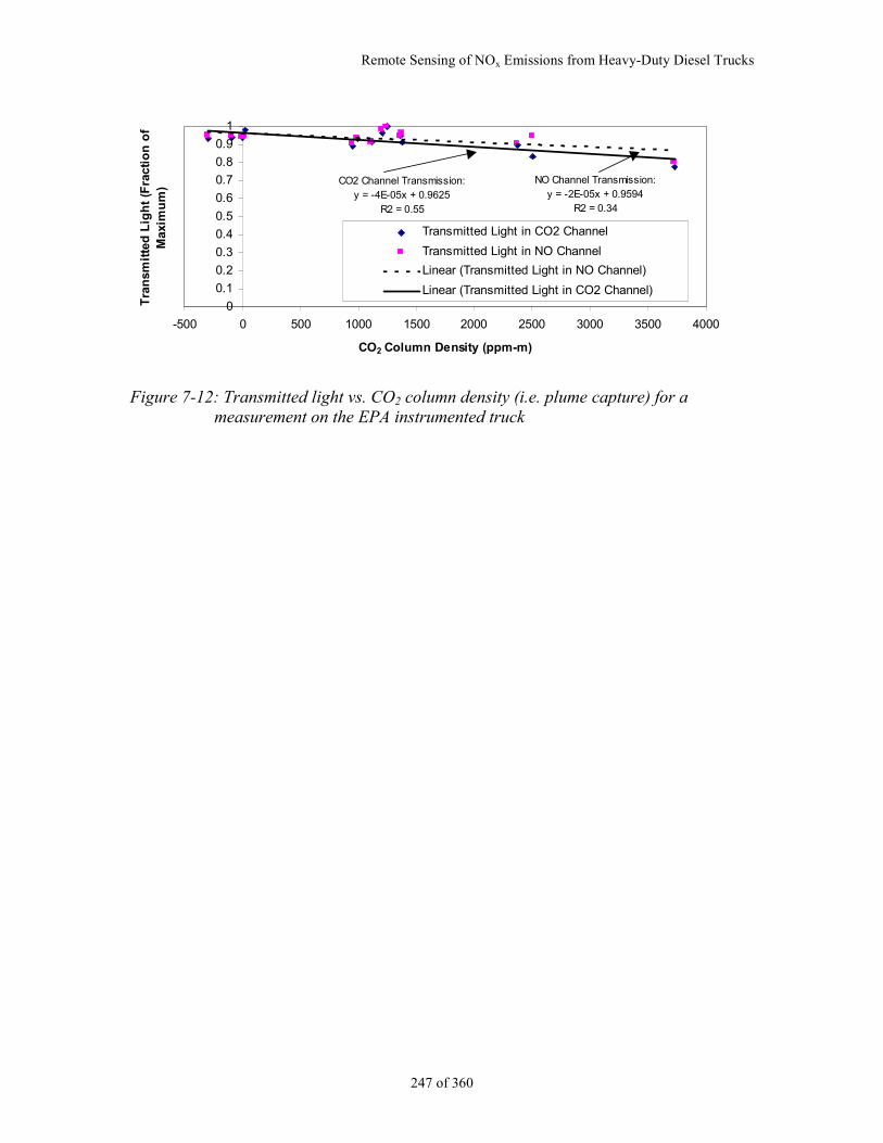
Remote Sensing of NOx Emissions from Heavy-Duty Diesel Trucks

247 of 360

NO Channel Transmission:y = -2E-05x + 0.9594

R2 = 0.34

CO2 Channel Transmission:y = -4E-05x + 0.9625

R2 = 0.55

0

0.1

0.2

0.3

0.4

0.5

0.6

0.7

0.8

0.9

1

-500 0 500 1000 1500 2000 2500 3000 3500 4000

CO2 Column Density (ppm-m)

Tra

nsm

itte

d L

igh

t (F

ract

ion

of

Max

imu

m)

Transmitted Light in CO2 Channel

Transmitted Light in NO Channel

Linear (Transmitted Light in NO Channel)

Linear (Transmitted Light in CO2 Channel)

Figure 7-12: Transmitted light vs. CO2 column density (i.e. plume capture) for ameasurement on the EPA instrumented truck

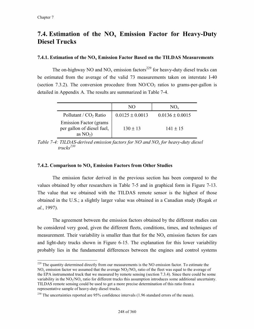
Chapter 7

248 of 360

7.4. Estimation of the NOx Emission Factor for Heavy-DutyDiesel Trucks

7.4.1. Estimation of the NOx Emission Factor Based on the TILDAS Measurements

The on-highway NO and NOx emission factors229 for heavy-duty diesel trucks can

be estimated from the average of the valid 73 measurements taken on interstate I-40

(section 7.3.2). The conversion procedure from NO/CO2 ratios to grams-per-gallon is

detailed in Appendix A. The results are summarized in Table 7-4.

NO NOx

Pollutant / CO2 Ratio 0.0125 ± 0.0013 0.0136 ± 0.0015

Emission Factor (gramsper gallon of diesel fuel,

as NO2)130 ± 13 141 ± 15

Table 7-4: TILDAS-derived emission factors for NO and NOx for heavy-duty dieseltrucks230

7.4.2. Comparison to NOx Emission Factors from Other Studies

The emission factor derived in the previous section has been compared to the

values obtained by other researchers in Table 7-5 and in graphical form in Figure 7-13.

The value that we obtained with the TILDAS remote sensor is the highest of those

obtained in the U.S.; a slightly larger value was obtained in a Canadian study (Rogak et

al., 1997).

The agreement between the emission factors obtained by the different studies can

be considered very good, given the different fleets, conditions, times, and techniques of

measurement. Their variability is smaller than that for the NOx emission factors for cars

and light-duty trucks shown in Figure 6-15. The explanation for this lower variability

probably lies in the fundamental differences between the engines and control systems

229 The quantity determined directly from our measurements is the NO emission factor. To estimate theNOx emission factor we assumed that the average NO2/NOx ratio of the fleet was equal to the average ofthe EPA instrumented truck that we measured by remote sensing (section 7.3.4). Since there could be somevariability in the NO2/NOx ratio for different trucks this assumption introduces some additional uncertainty.TILDAS remote sensing could be used to get a more precise determination of this ratio from arepresentative sample of heavy-duty diesel trucks.230 The uncertainties reported are 95% confidence intervals (1.96 standard errors of the mean).

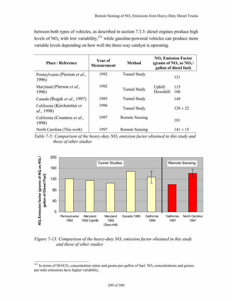
Remote Sensing of NOx Emissions from Heavy-Duty Diesel Trucks

249 of 360

between both types of vehicles, as described in section 7.3.3: diesel engines produce high

levels of NOx with low variability,231 while gasoline-powered vehicles can produce more

variable levels depending on how well the three-way catalyst is operating.

Place / ReferenceYear of

MeasurementMethod

NOx Emission Factor(grams of NOx as NO2 /

gallon of diesel fuel)

Pennsylvania (Pierson et al.,1996)

1992 Tunnel Study121

Maryland (Pierson et al.,1996)

1992Tunnel Study

Uphill: 115Downhill: 106

Canada (Rogak et al., 1997) 1995 Tunnel Study 149

California (Kirchstetter etal., 1998)

1996Tunnel Study 128 ± 22

California (Countess et al.,1998)

1997 Remote Sensing101

North Carolina (This work) 1997 Remote Sensing 141 ± 15

Table 7-5: Comparison of the heavy-duty NOx emission factor obtained in this study andthose of other studies

0

40

80

120

160

200

Pennsylvania1992

Maryland1992 (Uphill)

Maryland1992

(Dow nhill)

Canada 1995 California1996

California1997

North Carolina1997

NO

x E

mis

sio

n f

ac

tor

(gra

ms

of

NO

x a

s N

O2

/

ga

llon

of

Die

se

l Fu

el)

Tunnel Studies Remote Sensing

Figure 7-13: Comparison of the heavy-duty NOx emission factor obtained in this studyand those of other studies

231 In terms of NO/CO2 concentration ratios and grams-per-gallon of fuel. NOx concentrations and grams-per-mile emissions have higher variability.

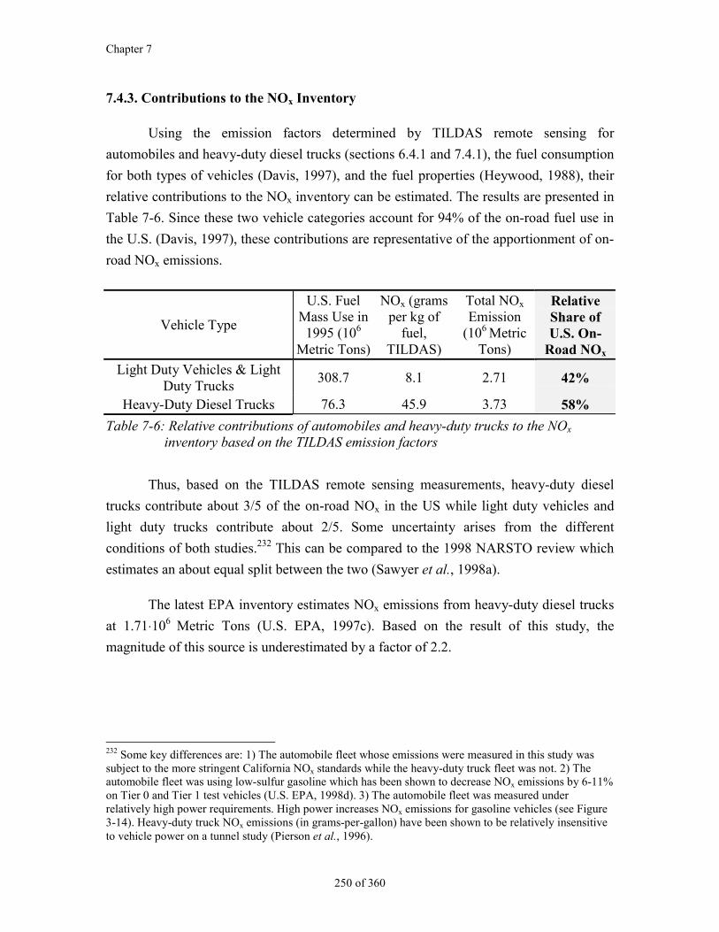
Chapter 7

250 of 360

7.4.3. Contributions to the NOx Inventory

Using the emission factors determined by TILDAS remote sensing for

automobiles and heavy-duty diesel trucks (sections 6.4.1 and 7.4.1), the fuel consumption

for both types of vehicles (Davis, 1997), and the fuel properties (Heywood, 1988), their

relative contributions to the NOx inventory can be estimated. The results are presented in

Table 7-6. Since these two vehicle categories account for 94% of the on-road fuel use in

the U.S. (Davis, 1997), these contributions are representative of the apportionment of on-

road NOx emissions.

Vehicle Type

U.S. FuelMass Use in

1995 (106

Metric Tons)

NOx (gramsper kg of

fuel,TILDAS)

Total NOx

Emission(106 Metric

Tons)

RelativeShare ofU.S. On-

Road NOx

Light Duty Vehicles & LightDuty Trucks

308.7 8.1 2.71 42%

Heavy-Duty Diesel Trucks 76.3 45.9 3.73 58%

Table 7-6: Relative contributions of automobiles and heavy-duty trucks to the NOx

inventory based on the TILDAS emission factors

Thus, based on the TILDAS remote sensing measurements, heavy-duty diesel

trucks contribute about 3/5 of the on-road NOx in the US while light duty vehicles and

light duty trucks contribute about 2/5. Some uncertainty arises from the different

conditions of both studies.232 This can be compared to the 1998 NARSTO review which

estimates an about equal split between the two (Sawyer et al., 1998a).

The latest EPA inventory estimates NOx emissions from heavy-duty diesel trucks

at 1.71⋅106 Metric Tons (U.S. EPA, 1997c). Based on the result of this study, the

magnitude of this source is underestimated by a factor of 2.2.

232 Some key differences are: 1) The automobile fleet whose emissions were measured in this study wassubject to the more stringent California NOx standards while the heavy-duty truck fleet was not. 2) Theautomobile fleet was using low-sulfur gasoline which has been shown to decrease NOx emissions by 6-11%on Tier 0 and Tier 1 test vehicles (U.S. EPA, 1998d). 3) The automobile fleet was measured underrelatively high power requirements. High power increases NOx emissions for gasoline vehicles (see Figure3-14). Heavy-duty truck NOx emissions (in grams-per-gallon) have been shown to be relatively insensitiveto vehicle power on a tunnel study (Pierson et al., 1996).

Remote Sensing of NOx Emissions from Heavy-Duty Diesel Trucks

251 of 360

7.5. Conclusions of this study

This study yielded a number of significant new findings with respect to remote

sensing of heavy-duty diesel truck (HDDT) emissions and their NOx emission factors.

The NOx emissions of HDDTs can be measured by TILDAS remote sensing under

real world conditions with very good accuracy and precision. Very good agreement

between the measurements of the EPA instrumented truck and the TILDAS

instrument was achieved.

Based on the results of this study the magnitude of HDDT NOx emissions is

underestimated by a factor of 2.2 in the U.S. The share of HDDTs on mobile source

NOx is larger than that of automobiles and light-duty trucks. The estimated

contribution of HDDTs to the NOx inventory supports the need for lower HDDT

emission standards now being implemented (U.S. EPA, 1997a). As much effort needs

to be done to reduce HDDT NOx emissions as has been done for light-duty vehicle

NOx, if further meaningful improvements in mobile source NOx-related air quality

problems are to be achieved.

The HDDT NOx emission factors are remarkably constant across several tunnel and

remote sensing studies. Thus the inventory contribution of HDDT NOx can be

reliably estimated from these emission factors.

The concept of “super-emitter” is not applicable to HDDTs for NOx, since the

differences between the lowest and the highest emitters are just a factor of 6.5,

compared to a factor of 750 for automobiles. Some consequences of this fact are:

− The potential of significant reductions on emissions through targeting an

inspection and maintenance program on the high emitters (or savings by

clean-screening low emitters) is small for HDDTs.

− Conversely, approaches that deal with the whole fleet such as emission

standards and reformulated diesel fuel have the largest potential.

The successful remote sensing of heavy-duty truck NOx opens the possibility of

exploring many interesting questions of the kind posed for automobile emissions on

Chapter 6 and previous studies. For example:

Chapter 7

252 of 360

− The fleet average emission factor for HDDTs can be determined under

real-world conditions under a variety of circumstances such as

geographical location, altitude, ambient temperature, roadway grade, etc.

These could be combined with the vehicle activity or fuel sales data to

produce a more accurate NOx emission inventory.

− The variation of HDDTs emissions vs. power can be studied. The concept

of specific power, defined in Chapter 3, is also applicable to HDDTs.

However, due to the very large variations in vehicle weight for these

vehicles, HDDT remote sensing studies should also obtain this

information.233

− The variation of emissions with vehicle age, manufacturer, engine family,

state or country of vehicle registration, vehicle operating company, etc.,

can be studied. This information can be used in the design of more

effective emission control strategies.

− By monitoring for a period of several years, the rates of deterioration as

well as the effects of emission reduction programs (such as diesel fuel

reformulation, low-NOx diesel engines, inspection and maintenance, etc.)

can be determined. This information can be invaluable for the design of

the next generation of emission control strategies.

233 This can be achieved by installing the remote sensing equipment at the exit of a weight station (Countesset al., 1998) or near a weight-in-motion system (U.S. DOT, 1997b).

253 of 360

Chapter 8. Remote Sensing of N2O Emissions fromAutomobiles and Light-Duty Trucks

8.1. Introduction

N2O emissions from motor vehicles are important due to their contribution to the increase

of the greenhouse effect and to stratospheric ozone depletion (Bouwman et al., 1995).

Concentrations of atmospheric N2O have been increasing at a rate of about 0.25% per

year, which has been attributed to human activities, although the relative contributions from the

different anthropogenic sources are still very uncertain (IPCC, 1995). Even though the rate of

increase of the N2O concentration in the atmosphere is three orders of magnitude lower than that

of CO2, the global warming potential of N2O is about 320 times larger than that of CO2 (IPCC,

1995), so the contributions of both gases to the increase of the greenhouse effect are of the same

order of magnitude. It has been estimated that to stabilize N2O concentrations at today's levels

would require reducing current rates of anthropogenic emission by more than 50% (IPCC,

1996a).

N2O is also involved in stratospheric ozone depletion. Since it is very inert in the

troposphere, N2O is slowly transported into the stratosphere where it is photolyzed and yields

NOx, which converts ozone into molecular oxygen. Approximately half of the ozone removal in

the stratosphere has been attributed to reactions of nitrogen oxides (Bowman, 1992).

Small amounts of N2O are formed in spark-ignition engines. Larger amounts of N2O may

be formed in automotive catalysts during NO reduction at relatively low temperatures. Catalyst

aging shifts the N2O production to higher catalyst temperatures, which occur more often during

typical driving. This causes an increase in N2O emissions.

Large uncertainties in the size of this N2O source remain. The 1998 EPA Draft

Greenhouse Gas Inventory (U.S. EPA, 1998c) estimated that this source could account for about

4% of the U.S. net greenhouse emissions. This was reported in the front page of the New York

Times (Wald, 1998) and caused significant controversy. The U.S. EPA Office of Mobile Sources

reacted by performing some additional N2O measurements and concluded that the source is

much smaller than the 1998 draft inventory suggested, although still highly uncertain (Michaels,

1998).

Chapter 8

254 of 360

This chapter presents the results of an N2O remote sensing campaign and a new

exhaustive compilation of the literature studies, in order to address some of the outstanding

questions about N2O emissions. The usefulness of remote sensing for estimation of N2O

emissions factors of on-road motor vehicles is evaluated first (section 8.2). The analysis of the

results of the remote sensing study performed in 1996 in California are presented later (sections

8.3 and 8.4). Section 8.5 presents the N2O emission factors determined in this study and a

comparison to those in the literature. The implications of the results and the analysis in this

chapter are summarized in section 8.6.

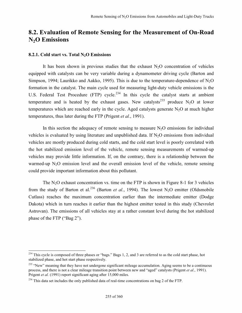
Remote Sensing of N2O Emissions from Automobiles and Light-Duty Trucks

255 of 360

8.2. Evaluation of Remote Sensing for the Measurement of On-RoadN2O Emissions

8.2.1. Cold start vs. Total N2O Emissions

It has been shown in previous studies that the exhaust N2O concentration of vehicles

equipped with catalysts can be very variable during a dynamometer driving cycle (Barton and

Simpson, 1994; Laurikko and Aakko, 1995). This is due to the temperature-dependence of N2O

formation in the catalyst. The main cycle used for measuring light-duty vehicle emissions is the

U.S. Federal Test Procedure (FTP) cycle.234 In this cycle the catalyst starts at ambient

temperature and is heated by the exhaust gases. New catalysts235 produce N2O at lower

temperatures which are reached early in the cycle. Aged catalysts generate N2O at much higher

temperatures, thus later during the FTP (Prigent et al., 1991).

In this section the adequacy of remote sensing to measure N2O emissions for individual

vehicles is evaluated by using literature and unpublished data. If N2O emissions from individual

vehicles are mostly produced during cold starts, and the cold start level is poorly correlated with

the hot stabilized emission level of the vehicle, remote sensing measurements of warmed-up

vehicles may provide little information. If, on the contrary, there is a relationship between the

warmed-up N2O emission level and the overall emission level of the vehicle, remote sensing

could provide important information about this pollutant.

The N2O exhaust concentration vs. time on the FTP is shown in Figure 8-1 for 3 vehicles

from the study of Barton et al.236 (Barton et al., 1994). The lowest N2O emitter (Oldsmobile

Cutlass) reaches the maximum concentration earlier than the intermediate emitter (Dodge

Dakota) which in turn reaches it earlier than the highest emitter tested in this study (Chevrolet

Astrovan). The emissions of all vehicles stay at a rather constant level during the hot stabilized

phase of the FTP (“Bag 2”).

234 This cycle is composed of three phases or “bags.” Bags 1, 2, and 3 are referred to as the cold start phase, hotstabilized phase, and hot start phase respectively.235 “New” meaning that they have not undergone significant mileage accumulation. Aging seems to be a continuousprocess, and there is not a clear mileage transition point between new and “aged” catalysts (Prigent et al., 1991).Prigent et al. (1991) report significant aging after 15,000 miles.236 This data set includes the only published data of real-time concentrations on bag 2 of the FTP.

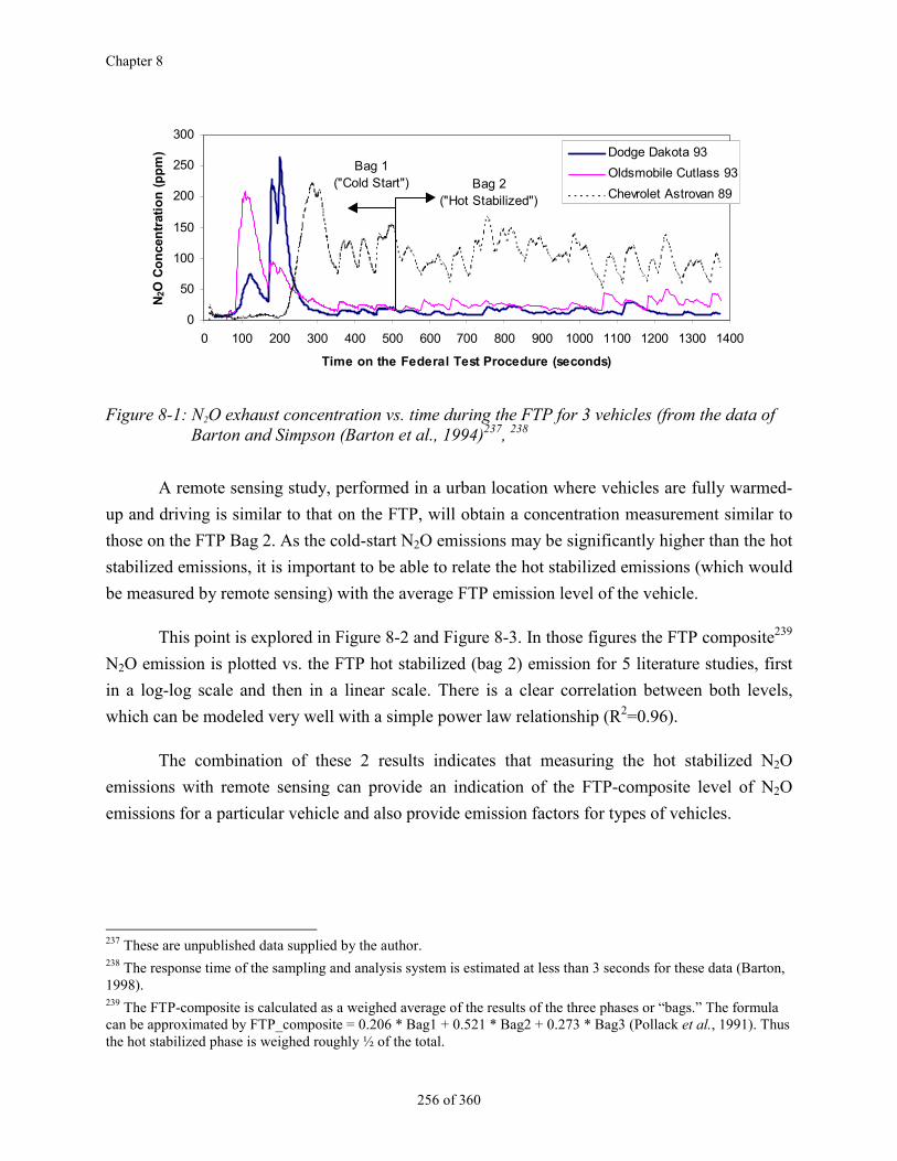
Chapter 8

256 of 360

0

50

100

150

200

250

300

0 100 200 300 400 500 600 700 800 900 1000 1100 1200 1300 1400

Time on the Federal Test Procedure (seconds)

N2O

Co

nce

ntr

atio

n (

pp

m) Dodge Dakota 93

Oldsmobile Cutlass 93

Chevrolet Astrovan 89

Bag 1("Cold Start") Bag 2

("Hot Stabilized")

Figure 8-1: N2O exhaust concentration vs. time during the FTP for 3 vehicles (from the data ofBarton and Simpson (Barton et al., 1994)237, 238

A remote sensing study, performed in a urban location where vehicles are fully warmed-

up and driving is similar to that on the FTP, will obtain a concentration measurement similar to

those on the FTP Bag 2. As the cold-start N2O emissions may be significantly higher than the hot

stabilized emissions, it is important to be able to relate the hot stabilized emissions (which would

be measured by remote sensing) with the average FTP emission level of the vehicle.

This point is explored in Figure 8-2 and Figure 8-3. In those figures the FTP composite239

N2O emission is plotted vs. the FTP hot stabilized (bag 2) emission for 5 literature studies, first

in a log-log scale and then in a linear scale. There is a clear correlation between both levels,

which can be modeled very well with a simple power law relationship (R2=0.96).

The combination of these 2 results indicates that measuring the hot stabilized N2O

emissions with remote sensing can provide an indication of the FTP-composite level of N2O

emissions for a particular vehicle and also provide emission factors for types of vehicles.

237 These are unpublished data supplied by the author.238 The response time of the sampling and analysis system is estimated at less than 3 seconds for these data (Barton,1998).239 The FTP-composite is calculated as a weighed average of the results of the three phases or “bags.” The formulacan be approximated by FTP_composite = 0.206 * Bag1 + 0.521 * Bag2 + 0.273 * Bag3 (Pollack et al., 1991). Thusthe hot stabilized phase is weighed roughly ½ of the total.

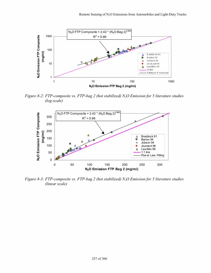
Remote Sensing of N2O Emissions from Automobiles and Light-Duty Trucks

257 of 360

1

10

100

1000

1 10 100 1000

N2O Emission FTP Bag 2 (mg/mi)

N2O

Em

iss

ion

FT

P C

om

po

sit

e

(mg

/mi)

B raddock 81

B arton 94

Jobson 94

Joum ard 96Laurikko 98

1:1 line

Fitting to P ower Law

N2O FTP Composite = 2.42 * (N2O Bag 2)0.863

R2 = 0.96

Figure 8-2: FTP-composite vs. FTP-bag 2 (hot stabilized) N2O Emission for 5 literature studies(log-scale)

0

50

100

150

200

250

300

0 50 100 150 200 250 300

N2O Emission FTP Bag 2 (mg/mi)

N2O

Em

issi

on

FT

P C

om

po

site

(mg

/mi)

Braddock 81Barton 94Jobson 94Joumard 96Laurikko 981:1 linePow er Law Fitting

N2O FTP Composite = 2.42 * (N2O Bag 2)0.863

R2 = 0.96

Figure 8-3: FTP-composite vs. FTP-bag 2 (hot stabilized) N2O Emission for 5 literature studies(linear scale)

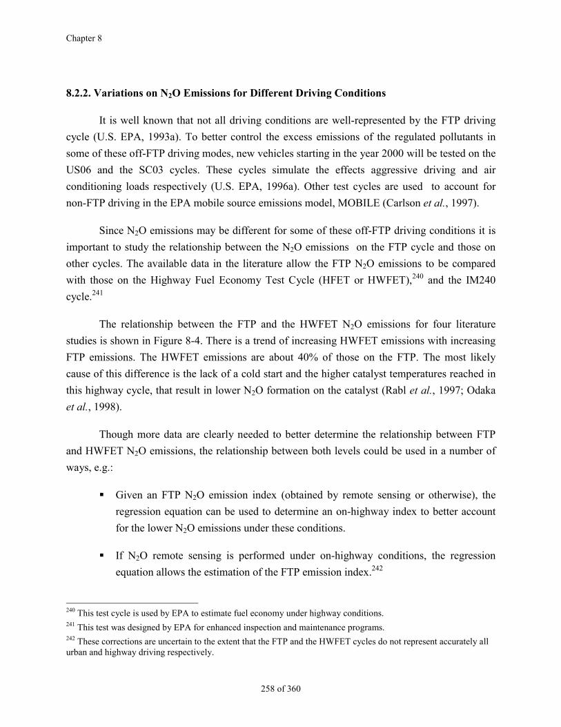
Chapter 8

258 of 360

8.2.2. Variations on N2O Emissions for Different Driving Conditions

It is well known that not all driving conditions are well-represented by the FTP driving

cycle (U.S. EPA, 1993a). To better control the excess emissions of the regulated pollutants in

some of these off-FTP driving modes, new vehicles starting in the year 2000 will be tested on the

US06 and the SC03 cycles. These cycles simulate the effects aggressive driving and air

conditioning loads respectively (U.S. EPA, 1996a). Other test cycles are used to account for

non-FTP driving in the EPA mobile source emissions model, MOBILE (Carlson et al., 1997).

Since N2O emissions may be different for some of these off-FTP driving conditions it is

important to study the relationship between the N2O emissions on the FTP cycle and those on

other cycles. The available data in the literature allow the FTP N2O emissions to be compared

with those on the Highway Fuel Economy Test Cycle (HFET or HWFET),240 and the IM240

cycle.241

The relationship between the FTP and the HWFET N2O emissions for four literature

studies is shown in Figure 8-4. There is a trend of increasing HWFET emissions with increasing

FTP emissions. The HWFET emissions are about 40% of those on the FTP. The most likely

cause of this difference is the lack of a cold start and the higher catalyst temperatures reached in

this highway cycle, that result in lower N2O formation on the catalyst (Rabl et al., 1997; Odaka

et al., 1998).

Though more data are clearly needed to better determine the relationship between FTP

and HWFET N2O emissions, the relationship between both levels could be used in a number of

ways, e.g.:

Given an FTP N2O emission index (obtained by remote sensing or otherwise), the

regression equation can be used to determine an on-highway index to better account

for the lower N2O emissions under these conditions.

If N2O remote sensing is performed under on-highway conditions, the regression

equation allows the estimation of the FTP emission index.242

240 This test cycle is used by EPA to estimate fuel economy under highway conditions.241 This test was designed by EPA for enhanced inspection and maintenance programs.242 These corrections are uncertain to the extent that the FTP and the HWFET cycles do not represent accurately allurban and highway driving respectively.

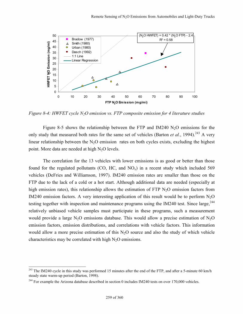
Remote Sensing of N2O Emissions from Automobiles and Light-Duty Trucks

259 of 360

0

5

10

15

20

25

30

35

40

45

50

0 10 20 30 40 50 60 70 80 90 100

FTP N2O Emission (mg/mi)

HW

FE

T N

2O

Em

issi

on

(m

g/m

i)

Bradow (1977)Smith (1980)Urban (1980)Dasch (1992)1:1 LineLinear Regression

(N2O HWFET) = 0.42 * (N2O FTP) - 2.4R2 = 0.58

Figure 8-4: HWFET cycle N2O emission vs. FTP composite emission for 4 literature studies

Figure 8-5 shows the relationship between the FTP and IM240 N2O emissions for the

only study that measured both rates for the same set of vehicles (Barton et al., 1994).243 A very

linear relationship between the N2O emission rates on both cycles exists, excluding the highest

point. More data are needed at high N2O levels.

The correlation for the 13 vehicles with lower emissions is as good or better than those

found for the regulated pollutants (CO, HC, and NOx) in a recent study which included 569

vehicles (DeFries and Williamson, 1997). IM240 emission rates are smaller than those on the

FTP due to the lack of a cold or a hot start. Although additional data are needed (especially at

high emission rates), this relationship allows the estimation of FTP N2O emission factors from

IM240 emission factors. A very interesting application of this result would be to perform N2O

testing together with inspection and maintenance programs using the IM240 test. Since large,244

relatively unbiased vehicle samples must participate in these programs, such a measurement

would provide a large N2O emissions database. This would allow a precise estimation of N2O

emission factors, emission distributions, and correlations with vehicle factors. This information

would allow a more precise estimation of this N2O source and also the study of which vehicle

characteristics may be correlated with high N2O emissions.

243 The IM240 cycle in this study was performed 15 minutes after the end of the FTP, and after a 5-minute 60 km/hsteady state warm-up period (Barton, 1998).244 For example the Arizona database described in section 0 includes IM240 tests on over 170,000 vehicles.

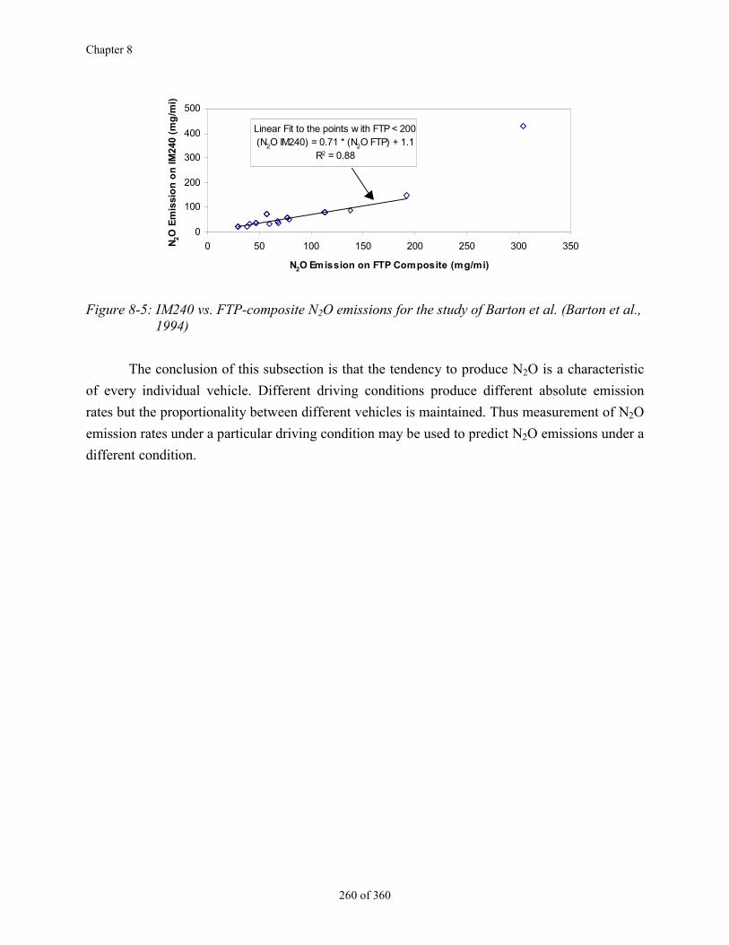
Chapter 8

260 of 360

Linear Fit to the points w ith FTP < 200(N2O IM240) = 0.71 * (N2O FTP) + 1.1

R2 = 0.88

0

100

200

300

400

500

0 50 100 150 200 250 300 350

N2O Emission on FTP Composite (mg/mi)

N2O

Em

issi

on

on

IM24

0 (m

g/m

i)

Figure 8-5: IM240 vs. FTP-composite N2O emissions for the study of Barton et al. (Barton et al.,1994)

The conclusion of this subsection is that the tendency to produce N2O is a characteristic

of every individual vehicle. Different driving conditions produce different absolute emission

rates but the proportionality between different vehicles is maintained. Thus measurement of N2O

emission rates under a particular driving condition may be used to predict N2O emissions under a

different condition.

Remote Sensing of N2O Emissions from Automobiles and Light-Duty Trucks

261 of 360

8.3. N2O Remote Sensing Results

8.3.1. Remote Sensing of N2O Emissions with TILDAS

The N2O emissions of automobiles and light-duty trucks were measured during our

experimental campaign in California in Nov. 1996 using the TILDAS technique. The details of

the experiments are presented in section 6.2. This technique had been used previously to monitor

N2O levels on directly sampled automotive exhaust (Jobson et al., 1994) and on directly sampled

aircraft gas turbine exhaust (Wiesen et al., 1996).

As explained in section 5.3, we were able to obtain N2O column densities with the same

laser used for determination of CO2 column densities by choosing a spectral region with strong,

non-overlapping N2O and CO2 transitions. The combined laser scan, time trace and N2O to CO2

regression are shown in Figure 5-4, Figure 5-5, and Figure 5-6 respectively. A small systematic

negative bias245 due to a beamsplitter fringe was detected and corrected for, as detailed on

Appendix E. We obtained a total of 1361 valid N2O emissions measurements in this way. The

analysis of these results is presented in the following sections.

8.3.2. N2O Emissions Distribution246

The statistics of the distribution of the N2O emissions are presented in Table 8-1. The

mean N2O emission value of the data set is 12.6 ± 3.95 ppm.247

A histogram of the distribution of the N2O emissions is presented in Figure 8-6. The

remote sensing N2O distribution is very skewed, with most of the readings at low emission

values and a long tail. The maximum reading is 245 ppm, which is well within the range of

concentrations reported in the literature, for example Prigent at al. (Prigent et al., 1994) report a 245 All of the analysis presented below has been performed after adding a constant value of +6.7 ppm to everyindividual data point, as estimated in Appendix E. The estimated uncertainty of the correction has not been added tothe data in this section since only the relative uncertainties are important here. It has been added to the comparisonof the emissions factors derived in this study with those of the literature (section 8.5.2) since in this case we arecomparing results of this study (which are subject to the uncertainty of the bias) with those of other studies (whichare not).246 The distribution of the emissions for all vehicles is presented here. The distributions for the individual vehicle /catalyst types are similar in shape with some differences in magnitude which are analyzed in the following sections.247 The uncertainty of the mean was calculated by adding in quadrature the standard error of the mean of ± 0.65 ppmand the estimate of the uncertainty on the magnitude of the systematic negative bias described in Appendix E (± 3.9ppm).

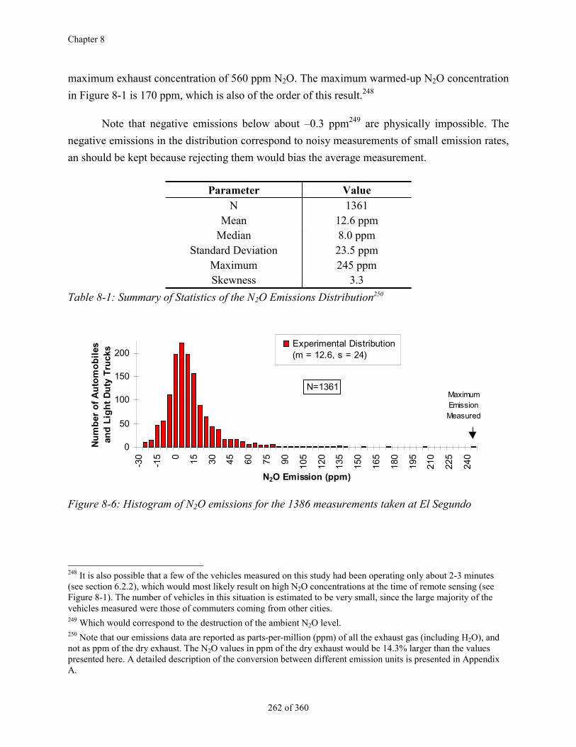
Chapter 8

262 of 360

maximum exhaust concentration of 560 ppm N2O. The maximum warmed-up N2O concentration

in Figure 8-1 is 170 ppm, which is also of the order of this result.248

Note that negative emissions below about –0.3 ppm249 are physically impossible. The

negative emissions in the distribution correspond to noisy measurements of small emission rates,

an should be kept because rejecting them would bias the average measurement.

Parameter ValueN 1361

Mean 12.6 ppmMedian 8.0 ppm

Standard Deviation 23.5 ppmMaximum 245 ppmSkewness 3.3

Table 8-1: Summary of Statistics of the N2O Emissions Distribution250

0

50

100

150

200

-30

-15 0 15 30 45 60 75 90 105

120

135

150

165

180

195

210

225

240

N2O Emission (ppm)

Nu

mb

er o

f A

uto

mo

bil

es

and

Lig

ht

Du

ty T

ruck

s Experimental Distribution(m = 12.6, s = 24)

MaximumEmissionMeasured

N=1361

Figure 8-6: Histogram of N2O emissions for the 1386 measurements taken at El Segundo

248 It is also possible that a few of the vehicles measured on this study had been operating only about 2-3 minutes(see section 6.2.2), which would most likely result on high N2O concentrations at the time of remote sensing (seeFigure 8-1). The number of vehicles in this situation is estimated to be very small, since the large majority of thevehicles measured were those of commuters coming from other cities.249 Which would correspond to the destruction of the ambient N2O level.250 Note that our emissions data are reported as parts-per-million (ppm) of all the exhaust gas (including H2O), andnot as ppm of the dry exhaust. The N2O values in ppm of the dry exhaust would be 14.3% larger than the valuespresented here. A detailed description of the conversion between different emission units is presented in AppendixA.

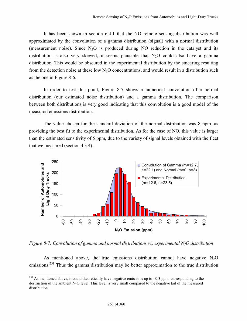
Remote Sensing of N2O Emissions from Automobiles and Light-Duty Trucks

263 of 360

It has been shown in section 6.4.1 that the NO remote sensing distribution was well

approximated by the convolution of a gamma distribution (signal) with a normal distribution

(measurement noise). Since N2O is produced during NO reduction in the catalyst and its

distribution is also very skewed, it seems plausible that N2O could also have a gamma

distribution. This would be obscured in the experimental distribution by the smearing resulting

from the detection noise at these low N2O concentrations, and would result in a distribution such

as the one in Figure 8-6.

In order to test this point, Figure 8-7 shows a numerical convolution of a normal

distribution (our estimated noise distribution) and a gamma distribution. The comparison

between both distributions is very good indicating that this convolution is a good model of the

measured emissions distribution.

The value chosen for the standard deviation of the normal distribution was 8 ppm, as

providing the best fit to the experimental distribution. As for the case of NO, this value is larger

than the estimated sensitivity of 5 ppm, due to the variety of signal levels obtained with the fleet

that we measured (section 4.3.4).

0

50

100

150

200

250

-60

-50

-40

-30

-20

-10 0 10 20 30 40 50 60 70 80 90 100

N2O Emission (ppm)

Nu

mb

er o

f A

uto

mo

bil

es a

nd

L

igh

t D

uty

Tru

cks

Convolution of Gamma (m=12.7,s=22.1) and Normal (m=0, s=8)

Experimental Distribution(m=12.6, s=23.5)

Figure 8-7: Convolution of gamma and normal distributions vs. experimental N2O distribution

As mentioned above, the true emissions distribution cannot have negative N2O

emissions.251 Thus the gamma distribution may be better approximation to the true distribution

251 As mentioned above, it could theoretically have negative emissions up to –0.3 ppm, corresponding to thedestruction of the ambient N2O level. This level is very small compared to the negative tail of the measureddistribution.

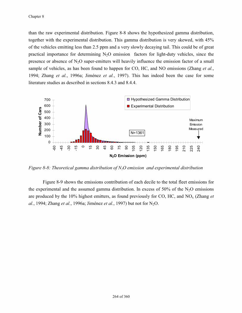
Chapter 8

264 of 360

than the raw experimental distribution. Figure 8-8 shows the hypothesized gamma distribution,

together with the experimental distribution. This gamma distribution is very skewed, with 45%

of the vehicles emitting less than 2.5 ppm and a very slowly decaying tail. This could be of great

practical importance for determining N2O emission factors for light-duty vehicles, since the

presence or absence of N2O super-emitters will heavily influence the emission factor of a small

sample of vehicles, as has been found to happen for CO, HC, and NO emissions (Zhang et al.,

1994; Zhang et al., 1996a; Jiménez et al., 1997). This has indeed been the case for some

literature studies as described in sections 8.4.3 and 8.4.4.

0

100

200

300

400

500

600

700

-60

-45

-30

-15 0

15

30

45

60

75

90

10

5

12

0

13

5

15

0

16

5

18

0

19

5

21

0

22

5

24

0

N2O Emission (ppm)

Nu

mb

er o

f C

ars

Hypothesized Gamma Distribution

Experimental Distribution

MaximumEmissionMeasured

N=1361

Figure 8-8: Theoretical gamma distribution of N2O emission and experimental distribution

Figure 8-9 shows the emissions contribution of each decile to the total fleet emissions for

the experimental and the assumed gamma distribution. In excess of 50% of the N2O emissions

are produced by the 10% highest emitters, as found previously for CO, HC, and NOx (Zhang et

al., 1994; Zhang et al., 1996a; Jiménez et al., 1997) but not for N2O.

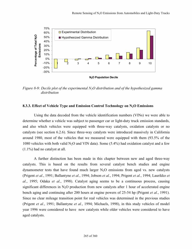
Remote Sensing of N2O Emissions from Automobiles and Light-Duty Trucks

265 of 360

-30%

-20%

-10%

0%

10%

20%

30%

40%

50%

60%

70%

1 2 3 4 5 6 7 8 9 10

N2O Population Decile

Pe

rce

nta

ge

of

To

tal N

2O

Em

iss

ion

s

Experimental Distribution

Hypothesized Gamma Distribution

Figure 8-9: Decile plot of the experimental N2O distribution and of the hypothesized gammadistribution

8.3.3. Effect of Vehicle Type and Emission Control Technology on N2O Emissions

Using the data decoded from the vehicle identification numbers (VINs) we were able to

determine whether a vehicle was subject to passenger car or light-duty truck emission standards,

and also which vehicles were equipped with three-way catalysts, oxidation catalysts or no

catalysts (see section 6.2.6). Since three-way catalysts were introduced massively in California

around 1980, most of the vehicles that we measured were equipped with them (93.5% of the

1080 vehicles with both valid N2O and VIN data). Some (5.4%) had oxidation catalyst and a few

(1.1%) had no catalyst at all.

A further distinction has been made in this chapter between new and aged three-way

catalysts. This is based on the results from several catalyst bench studies and engine

dynamometer tests that have found much larger N2O emissions from aged vs. new catalysts

(Prigent et al., 1991; Ballantyne et al., 1994; Jobson et al., 1994; Prigent et al., 1994; Laurikko et

al., 1995; Odaka et al., 1998). Catalyst aging seems to be a continuous process, causing

significant differences in N2O production from new catalysts after 1 hour of accelerated engine

bench aging and continuing after 200 hours at engine powers of 25-54 hp (Prigent et al., 1991).

Since no clear mileage transition point for real vehicles was determined in the previous studies

(Prigent et al., 1991; Ballantyne et al., 1994; Michaels, 1998), in this study vehicles of model

year 1996 were considered to have new catalysts while older vehicles were considered to have

aged catalysts.

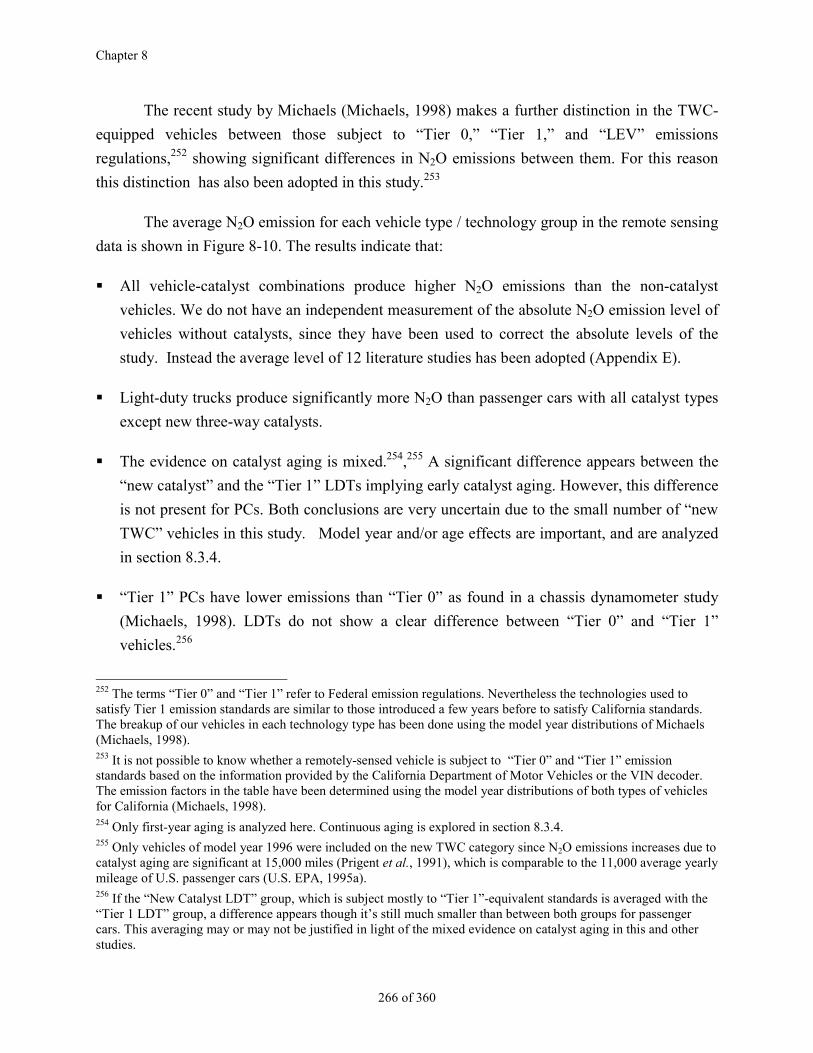
Chapter 8

266 of 360

The recent study by Michaels (Michaels, 1998) makes a further distinction in the TWC-

equipped vehicles between those subject to “Tier 0,” “Tier 1,” and “LEV” emissions

regulations,252 showing significant differences in N2O emissions between them. For this reason

this distinction has also been adopted in this study.253

The average N2O emission for each vehicle type / technology group in the remote sensing

data is shown in Figure 8-10. The results indicate that:

All vehicle-catalyst combinations produce higher N2O emissions than the non-catalyst

vehicles. We do not have an independent measurement of the absolute N2O emission level of

vehicles without catalysts, since they have been used to correct the absolute levels of the

study. Instead the average level of 12 literature studies has been adopted (Appendix E).

Light-duty trucks produce significantly more N2O than passenger cars with all catalyst types

except new three-way catalysts.

The evidence on catalyst aging is mixed.254,255 A significant difference appears between the

“new catalyst” and the “Tier 1” LDTs implying early catalyst aging. However, this difference

is not present for PCs. Both conclusions are very uncertain due to the small number of “new

TWC” vehicles in this study. Model year and/or age effects are important, and are analyzed

in section 8.3.4.

“Tier 1” PCs have lower emissions than “Tier 0” as found in a chassis dynamometer study

(Michaels, 1998). LDTs do not show a clear difference between “Tier 0” and “Tier 1”

vehicles.256

252 The terms “Tier 0” and “Tier 1” refer to Federal emission regulations. Nevertheless the technologies used tosatisfy Tier 1 emission standards are similar to those introduced a few years before to satisfy California standards.The breakup of our vehicles in each technology type has been done using the model year distributions of Michaels(Michaels, 1998).253 It is not possible to know whether a remotely-sensed vehicle is subject to “Tier 0” and “Tier 1” emissionstandards based on the information provided by the California Department of Motor Vehicles or the VIN decoder.The emission factors in the table have been determined using the model year distributions of both types of vehiclesfor California (Michaels, 1998).254 Only first-year aging is analyzed here. Continuous aging is explored in section 8.3.4.255 Only vehicles of model year 1996 were included on the new TWC category since N2O emissions increases due tocatalyst aging are significant at 15,000 miles (Prigent et al., 1991), which is comparable to the 11,000 average yearlymileage of U.S. passenger cars (U.S. EPA, 1995a).256 If the “New Catalyst LDT” group, which is subject mostly to “Tier 1”-equivalent standards is averaged with the“Tier 1 LDT” group, a difference appears though it’s still much smaller than between both groups for passengercars. This averaging may or may not be justified in light of the mixed evidence on catalyst aging in this and otherstudies.

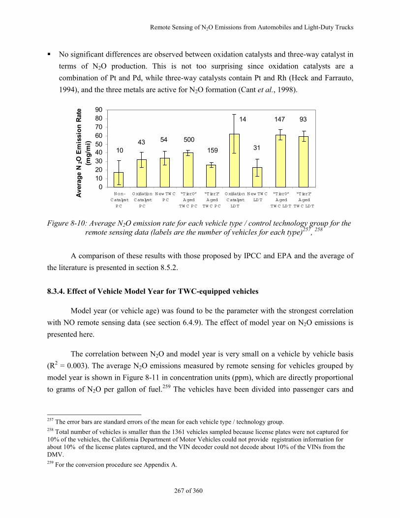
Remote Sensing of N2O Emissions from Automobiles and Light-Duty Trucks

267 of 360

No significant differences are observed between oxidation catalysts and three-way catalyst in

terms of N2O production. This is not too surprising since oxidation catalysts are a

combination of Pt and Pd, while three-way catalysts contain Pt and Rh (Heck and Farrauto,

1994), and the three metals are active for N2O formation (Cant et al., 1998).

0102030405060708090

Non-

Catalyst

PC

Oxidation

Catalyst

PC

New TW C

PC

“Tier 0”

Aged

TW C PC

“Tier 1”

Aged

TW C PC

Oxidation

Catalyst

LD T

New TW C

LD T

“Tier 0”

Aged

TW C LD T

“Tier 1”

Aged

TW C LD T

Ave

rag

e N

2O E

mis

sio

n R

ate

(mg

/mi)

1043

14

54 500

159

147 93

31

Figure 8-10: Average N2O emission rate for each vehicle type / control technology group for theremote sensing data (labels are the number of vehicles for each type)257, 258

A comparison of these results with those proposed by IPCC and EPA and the average of

the literature is presented in section 8.5.2.

8.3.4. Effect of Vehicle Model Year for TWC-equipped vehicles

Model year (or vehicle age) was found to be the parameter with the strongest correlation

with NO remote sensing data (see section 6.4.9). The effect of model year on N2O emissions is

presented here.

The correlation between N2O and model year is very small on a vehicle by vehicle basis

(R2 = 0.003). The average N2O emissions measured by remote sensing for vehicles grouped by

model year is shown in Figure 8-11 in concentration units (ppm), which are directly proportional

to grams of N2O per gallon of fuel.259 The vehicles have been divided into passenger cars and

257 The error bars are standard errors of the mean for each vehicle type / technology group.258 Total number of vehicles is smaller than the 1361 vehicles sampled because license plates were not captured for10% of the vehicles, the California Department of Motor Vehicles could not provide registration information forabout 10% of the license plates captured, and the VIN decoder could not decode about 10% of the VINs from theDMV.259 For the conversion procedure see Appendix A.

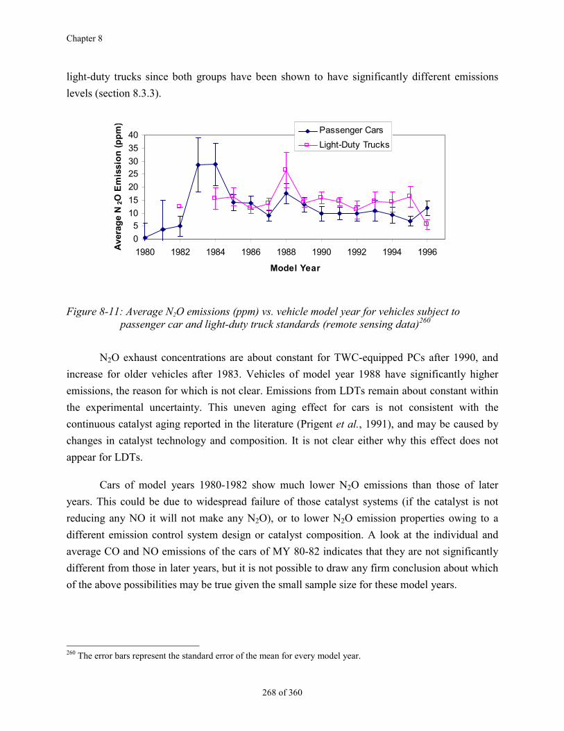
Chapter 8

268 of 360

light-duty trucks since both groups have been shown to have significantly different emissions

levels (section 8.3.3).

0

5

10

15

20

25

30

35

40

1980 1982 1984 1986 1988 1990 1992 1994 1996

Model Year

Ave

rag

e N

2O E

mis

sio

n (

pp

m)

Passenger Cars

Light-Duty Trucks

Figure 8-11: Average N2O emissions (ppm) vs. vehicle model year for vehicles subject topassenger car and light-duty truck standards (remote sensing data)260

N2O exhaust concentrations are about constant for TWC-equipped PCs after 1990, and

increase for older vehicles after 1983. Vehicles of model year 1988 have significantly higher

emissions, the reason for which is not clear. Emissions from LDTs remain about constant within

the experimental uncertainty. This uneven aging effect for cars is not consistent with the

continuous catalyst aging reported in the literature (Prigent et al., 1991), and may be caused by

changes in catalyst technology and composition. It is not clear either why this effect does not

appear for LDTs.

Cars of model years 1980-1982 show much lower N2O emissions than those of later

years. This could be due to widespread failure of those catalyst systems (if the catalyst is not

reducing any NO it will not make any N2O), or to lower N2O emission properties owing to a

different emission control system design or catalyst composition. A look at the individual and

average CO and NO emissions of the cars of MY 80-82 indicates that they are not significantly

different from those in later years, but it is not possible to draw any firm conclusion about which

of the above possibilities may be true given the small sample size for these model years.

260 The error bars represent the standard error of the mean for every model year.

Remote Sensing of N2O Emissions from Automobiles and Light-Duty Trucks

269 of 360

0

20

40

60

80

100

120

140

1980 1982 1984 1986 1988 1990 1992 1994 1996

Model Year

Ave

rag

e N

2O E

mis

sio

n (

mg

/mi)

Passenger Cars

Light-Duty Trucks

Figure 8-12: Average N2O emissions (mg/mi) vs. vehicle model year for vehicles subject topassenger car and light-duty truck standards (remote sensing data)

Figure 8-12 shows the same results in emission rate units, mg/mi. The difference between

PCs and LDTs is significantly larger than in grams-per-gallon units for most model years. This

result indicates that about half of the difference in the N2O emission rates between both types of

vehicles is due to the difference in fuel economies, and that light-duty trucks also tend to

generate more N2O per unit fuel consumed.261

8.3.5. Fraction of Total Emissions Contributed by Every Model Year (TWC only)

The fraction of the total N2O emissions for every model year has been calculated by

adding the emissions of each vehicle observed at every model year and dividing by the sum of

the total emissions. The results of this procedure are shown in Figure 8-13.

All model years from 1984 on contribute very similar fractions of about 7% of the total

N2O. This results from the slight increase in emissions compensating the decrease in the vehicle

population. Passenger cars are the dominant contributor for older model years and light-duty

trucks become equal or larger from 1990 on, due to the increase in the number of trucks as a

fraction of the fleet.

261 The possible reasons for the higher N2O emission per unit fuel for LDTs are unclear. Some possibilities includeincreased catalyst aging due to more aggressive driving, slightly lower average catalyst temperatures due todifferences in exhaust system design and mass flows, or differences in catalyst loading and/or composition withrespect to passenger cars.

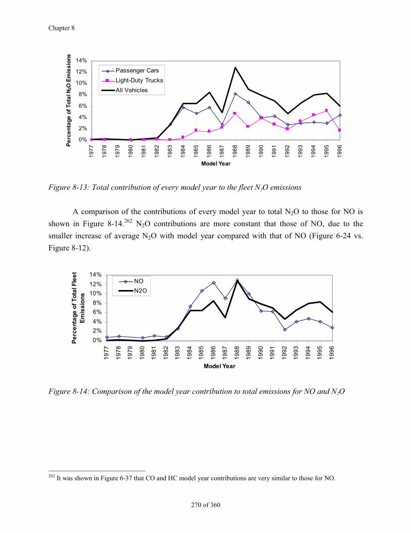
Chapter 8

270 of 360

0%

2%

4%

6%

8%

10%

12%

14%

19

77

19

78

19

79

19

80

19

81

19

82

19

83

19

84

19

85

19

86

19

87

19

88

19

89

19

90

19

91

19

92

19

93

19

94

19

95

19

96

Model Year

Pe

rce

nta

ge

of

To

tal N

2O E

mis

sio

ns

Passenger Cars

Light-Duty Trucks

All Vehicles

Figure 8-13: Total contribution of every model year to the fleet N2O emissions

A comparison of the contributions of every model year to total N2O to those for NO is

shown in Figure 8-14.262 N2O contributions are more constant that those of NO, due to the

smaller increase of average N2O with model year compared with that of NO (Figure 6-24 vs.

Figure 8-12).

0%

2%

4%

6%

8%

10%

12%

14%

19

77

19

78

19

79

19

80

19

81

19

82

19

83

19

84

19

85

19

86

19

87

19

88

19

89

19

90

19

91

19

92

19

93

19

94

19

95

19

96

Model Year

Pe

rce

nta

ge

of

To

tal F

lee

t E

mis

sio

ns

NO

N2O

Figure 8-14: Comparison of the model year contribution to total emissions for NO and N2O

262 It was shown in Figure 6-37 that CO and HC model year contributions are very similar to those for NO.

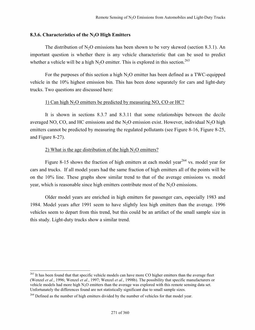
Remote Sensing of N2O Emissions from Automobiles and Light-Duty Trucks

271 of 360

8.3.6. Characteristics of the N2O High Emitters

The distribution of N2O emissions has been shown to be very skewed (section 8.3.1). An

important question is whether there is any vehicle characteristic that can be used to predict

whether a vehicle will be a high N2O emitter. This is explored in this section.263

For the purposes of this section a high N2O emitter has been defined as a TWC-equipped

vehicle in the 10% highest emission bin. This has been done separately for cars and light-duty

trucks. Two questions are discussed here:

1) Can high N2O emitters be predicted by measuring NO, CO or HC?

It is shown in sections 8.3.7 and 8.3.11 that some relationships between the decile

averaged NO, CO, and HC emissions and the N2O emission exist. However, individual N2O high

emitters cannot be predicted by measuring the regulated pollutants (see Figure 8-16, Figure 8-25,

and Figure 8-27).

2) What is the age distribution of the high N2O emitters?

Figure 8-15 shows the fraction of high emitters at each model year264 vs. model year for

cars and trucks. If all model years had the same fraction of high emitters all of the points will be

on the 10% line. These graphs show similar trend to that of the average emissions vs. model

year, which is reasonable since high emitters contribute most of the N2O emissions.

Older model years are enriched in high emitters for passenger cars, especially 1983 and

1984. Model years after 1991 seem to have slightly less high emitters than the average. 1996

vehicles seem to depart from this trend, but this could be an artifact of the small sample size in

this study. Light-duty trucks show a similar trend.

263 It has been found that that specific vehicle models can have more CO higher emitters than the average fleet(Wenzel et al., 1996; Wenzel et al., 1997; Wenzel et al., 1998b). The possibility that specific manufacturers orvehicle models had more high N2O emitters than the average was explored with this remote sensing data set.Unfortunately the differences found are not statistically significant due to small sample sizes.264 Defined as the number of high emitters divided by the number of vehicles for that model year.

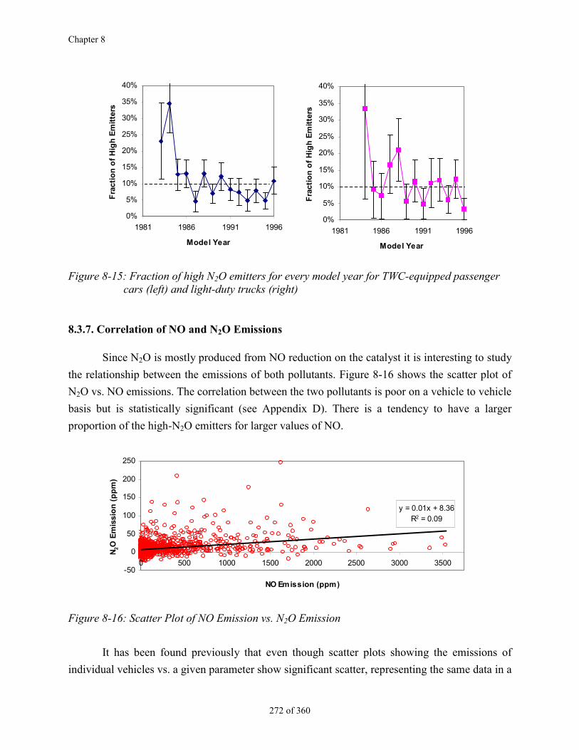
Chapter 8

272 of 360

0%

5%

10%

15%

20%

25%

30%

35%

40%

1981 1986 1991 1996

Model Year

Fra

ctio

n o

f H

igh

Em

itte

rs

0%

5%

10%

15%

20%

25%

30%

35%

40%

1981 1986 1991 1996

Model Year

Fra

ctio

n o

f H

igh

Em

itte

rs

Figure 8-15: Fraction of high N2O emitters for every model year for TWC-equipped passengercars (left) and light-duty trucks (right)

8.3.7. Correlation of NO and N2O Emissions

Since N2O is mostly produced from NO reduction on the catalyst it is interesting to study

the relationship between the emissions of both pollutants. Figure 8-16 shows the scatter plot of

N2O vs. NO emissions. The correlation between the two pollutants is poor on a vehicle to vehicle

basis but is statistically significant (see Appendix D). There is a tendency to have a larger

proportion of the high-N2O emitters for larger values of NO.

y = 0.01x + 8.36R2 = 0.09

-50

0

50

100

150

200

250

0 500 1000 1500 2000 2500 3000 3500

NO Emission (ppm)

N2O

Em

issi

on

(p

pm

)

Figure 8-16: Scatter Plot of NO Emission vs. N2O Emission

It has been found previously that even though scatter plots showing the emissions of

individual vehicles vs. a given parameter show significant scatter, representing the same data in a

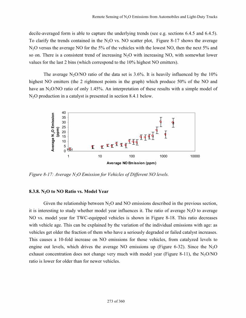
Remote Sensing of N2O Emissions from Automobiles and Light-Duty Trucks

273 of 360

decile-averaged form is able to capture the underlying trends (see e.g. sections 6.4.5 and 6.4.5).

To clarify the trends contained in the N2O vs. NO scatter plot, Figure 8-17 shows the average

N2O versus the average NO for the 5% of the vehicles with the lowest NO, then the next 5% and

so on. There is a consistent trend of increasing N2O with increasing NO, with somewhat lower

values for the last 2 bins (which correspond to the 10% highest NO emitters).

The average N2O/NO ratio of the data set is 3.6%. It is heavily influenced by the 10%

highest NO emitters (the 2 rightmost points in the graph) which produce 50% of the NO and

have an N2O/NO ratio of only 1.45%. An interpretation of these results with a simple model of

N2O production in a catalyst is presented in section 8.4.1 below.

05

10152025303540

1 10 100 1000 10000

Average NO Emission (ppm)

Ave

rag

e N

2O E

mis

sio

n

(pp

m)

Figure 8-17: Average N2O Emission for Vehicles of Different NO levels.

8.3.8. N2O to NO Ratio vs. Model Year

Given the relationship between N2O and NO emissions described in the previous section,

it is interesting to study whether model year influences it. The ratio of average N2O to average

NO vs. model year for TWC-equipped vehicles is shown in Figure 8-18. This ratio decreases

with vehicle age. This can be explained by the variation of the individual emissions with age: as

vehicles get older the fraction of them who have a seriously degraded or failed catalyst increases.

This causes a 10-fold increase on NO emissions for those vehicles, from catalyzed levels to

engine out levels, which drives the average NO emissions up (Figure 6-32). Since the N2O

exhaust concentration does not change very much with model year (Figure 8-11), the N2O/NO

ratio is lower for older than for newer vehicles.

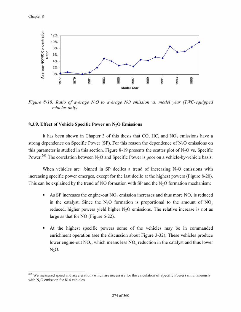
Chapter 8

274 of 360

0%

2%

4%

6%

8%

10%

12%

19

77

19

79

19

81

19

83

19

85

19

87

19

89

19

91

19

93

19

95

Model Year

Av

era

ge

N2O

/NO

Co

nc

en

tra

tio

n

Ra

tio

Figure 8-18: Ratio of average N2O to average NO emission vs. model year (TWC-equippedvehicles only)

8.3.9. Effect of Vehicle Specific Power on N2O Emissions

It has been shown in Chapter 3 of this thesis that CO, HC, and NOx emissions have a

strong dependence on Specific Power (SP). For this reason the dependence of N2O emissions on

this parameter is studied in this section. Figure 8-19 presents the scatter plot of N2O vs. Specific

Power.265 The correlation between N2O and Specific Power is poor on a vehicle-by-vehicle basis.

When vehicles are binned in SP deciles a trend of increasing N2O emissions with

increasing specific power emerges, except for the last decile at the highest powers (Figure 8-20).

This can be explained by the trend of NO formation with SP and the N2O formation mechanism:

As SP increases the engine-out NOx emission increases and thus more NOx is reduced

in the catalyst. Since the N2O formation is proportional to the amount of NOx

reduced, higher powers yield higher N2O emissions. The relative increase is not as

large as that for NO (Figure 6-22).

At the highest specific powers some of the vehicles may be in commanded

enrichment operation (see the discussion about Figure 3-32). These vehicles produce

lower engine-out NOx, which means less NOx reduction in the catalyst and thus lower

N2O.

265 We measured speed and acceleration (which are necessary for the calculation of Specific Power) simultaneouslywith N2O emission for 814 vehicles.

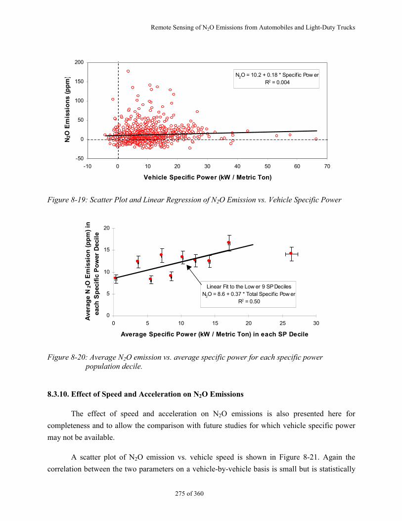
Remote Sensing of N2O Emissions from Automobiles and Light-Duty Trucks

275 of 360

N2O = 10.2 + 0.18 * Specif ic Pow erR2 = 0.004

-50

0

50

100

150

200

-10 0 10 20 30 40 50 60 70

Vehicle Specific Power (kW / Metric Ton)

N2O

Em

issi

on

s (p

pm

)

Figure 8-19: Scatter Plot and Linear Regression of N2O Emission vs. Vehicle Specific Power

Linear Fit to the Low er 9 SP DecilesN2O = 8.6 + 0.37 * Total Specif ic Pow er

R2 = 0.50

0

5

10

15

20

0 5 10 15 20 25 30

Average Specific Power (kW / Metric Ton) in each SP Decile

Ave

rag

e N

2O

Em

issi

on

(p

pm

) in

each

Sp

ecif

ic P

ow

er D

ecil

e

Figure 8-20: Average N2O emission vs. average specific power for each specific powerpopulation decile.

8.3.10. Effect of Speed and Acceleration on N2O Emissions

The effect of speed and acceleration on N2O emissions is also presented here for

completeness and to allow the comparison with future studies for which vehicle specific power

may not be available.

A scatter plot of N2O emission vs. vehicle speed is shown in Figure 8-21. Again the

correlation between the two parameters on a vehicle-by-vehicle basis is small but is statistically

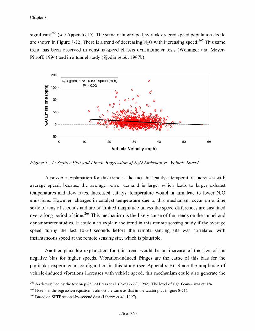
Chapter 8

276 of 360

significant266 (see Appendix D). The same data grouped by rank ordered speed population decile

are shown in Figure 8-22. There is a trend of decreasing N2O with increasing speed.267 This same

trend has been observed in constant-speed chassis dynamometer tests (Wehinger and Meyer-

Pitroff, 1994) and in a tunnel study (Sjödin et al., 1997b).

N2O (ppm) = 28 - 0.50 * Speed (mph)R2 = 0.02

-50

0

50

100

150

200

0 10 20 30 40 50 60

Vehicle Velocity (mph)

N2O

Em

issi

on

s (p

pm

)

Figure 8-21: Scatter Plot and Linear Regression of N2O Emission vs. Vehicle Speed

A possible explanation for this trend is the fact that catalyst temperature increases with

average speed, because the average power demand is larger which leads to larger exhaust

temperatures and flow rates. Increased catalyst temperature would in turn lead to lower N2O

emissions. However, changes in catalyst temperature due to this mechanism occur on a time

scale of tens of seconds and are of limited magnitude unless the speed differences are sustained

over a long period of time.268 This mechanism is the likely cause of the trends on the tunnel and

dynamometer studies. It could also explain the trend in this remote sensing study if the average

speed during the last 10-20 seconds before the remote sensing site was correlated with

instantaneous speed at the remote sensing site, which is plausible.

Another plausible explanation for this trend would be an increase of the size of the

negative bias for higher speeds. Vibration-induced fringes are the cause of this bias for the

particular experimental configuration in this study (see Appendix E). Since the amplitude of

vehicle-induced vibrations increases with vehicle speed, this mechanism could also generate the 266 As determined by the test on p.636 of Press et al. (Press et al., 1992). The level of significance was α=1%.267 Note that the regression equation is almost the same as that in the scatter plot (Figure 8-21).268 Based on SFTP second-by-second data (Liberty et al., 1997).

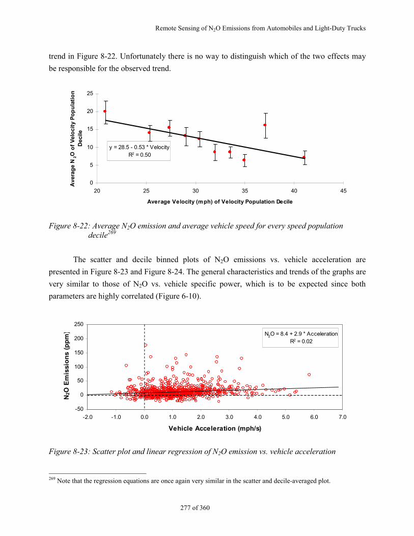
Remote Sensing of N2O Emissions from Automobiles and Light-Duty Trucks

277 of 360

trend in Figure 8-22. Unfortunately there is no way to distinguish which of the two effects may

be responsible for the observed trend.

y = 28.5 - 0.53 * VelocityR2 = 0.50

0

5

10

15

20

25

20 25 30 35 40 45

Average Velocity (mph) of Velocity Population Decile

Ave

rag

e N

2O

of

Vel

oci

ty P

op

ula

tio

n

Dec

ile

Figure 8-22: Average N2O emission and average vehicle speed for every speed populationdecile269

The scatter and decile binned plots of N2O emissions vs. vehicle acceleration are

presented in Figure 8-23 and Figure 8-24. The general characteristics and trends of the graphs are

very similar to those of N2O vs. vehicle specific power, which is to be expected since both

parameters are highly correlated (Figure 6-10).

N2O = 8.4 + 2.9 * AccelerationR2 = 0.02

-50

0

50

100

150

200

250

-2.0 -1.0 0.0 1.0 2.0 3.0 4.0 5.0 6.0 7.0

Vehicle Acceleration (mph/s)

N2O

Em

issi

on

s (p

pm

)

Figure 8-23: Scatter plot and linear regression of N2O emission vs. vehicle acceleration

269 Note that the regression equations are once again very similar in the scatter and decile-averaged plot.

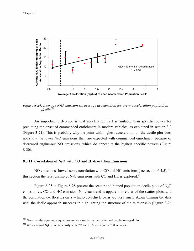
Chapter 8

278 of 360

N2O = 10.6 + 3.1 * AccelerationR2 = 0.59

0

5

10

15

20

25

-0.5 0 0.5 1 1.5 2 2.5 3 3.5 4

Average Acceleration (mph/s) of each Acceleration Population Decile

Ave

rag

e N

2O

Em

issi

on

(p

pm

) o

f ea

ch

Acc

eler

atio

n P

op

ula

tio

n D

ecile

Figure 8-24: Average N2O emission vs. average acceleration for every acceleration populationdecile270

An important difference is that acceleration is less suitable than specific power for

predicting the onset of commanded enrichment in modern vehicles, as explained in section 3.2

(Figure 3-21). This is probably why the point with highest acceleration on the decile plot does

not show the lower N2O emissions that are expected with commanded enrichment because of

decreased engine-out NO emissions, which do appear at the highest specific powers (Figure

8-20).

8.3.11. Correlation of N2O with CO and Hydrocarbon Emissions

NO emissions showed some correlation with CO and HC emissions (see section 6.4.5). In

this section the relationship of N2O emissions with CO and HC is explored.271

Figure 8-25 to Figure 8-28 present the scatter and binned population decile plots of N2O

emission vs. CO and HC emission. No clear trend is apparent in either of the scatter plots, and

the correlation coefficients on a vehicle-by-vehicle basis are very small. Again binning the data

with the decile approach succeeds in highlighting the structure of the relationship (Figure 8-26

270 Note that the regression equations are very similar in the scatter and decile-averaged plot.271 We measured N2O simultaneously with CO and HC emission for 780 vehicles.

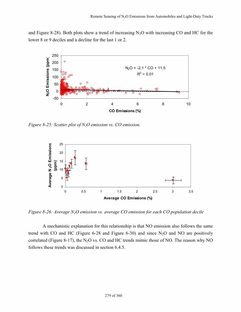
Remote Sensing of N2O Emissions from Automobiles and Light-Duty Trucks

279 of 360

and Figure 8-28). Both plots show a trend of increasing N2O with increasing CO and HC for the

lower 8 or 9 deciles and a decline for the last 1 or 2.

N2O = -2.1 * CO + 11.5

R2 = 0.01

-50

0

50

100

150

200

250

0 2 4 6 8 10

CO Emissions (%)

N2O

Em

issi

on

s (p

pm

)

Figure 8-25: Scatter plot of N2O emission vs. CO emission.

0

5

10

15

20

25

0 0.5 1 1.5 2 2.5 3 3.5

Average CO Emissions (%)

Ave

rag

e N

2O

Em

issi

on

s(p

pm

)

Figure 8-26: Average N2O emission vs. average CO emission for each CO population decile

A mechanistic explanation for this relationship is that NO emission also follows the same

trend with CO and HC (Figure 6-28 and Figure 6-30) and since N2O and NO are positively

correlated (Figure 8-17), the N2O vs. CO and HC trends mimic those of NO. The reason why NO

follows these trends was discussed in section 6.4.5.

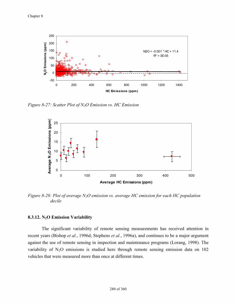
Chapter 8

280 of 360

N2O = -0.001 * HC + 11.4R2 = 3E-05

-50

0

50

100

150

200

250

0 200 400 600 800 1000 1200 1400

HC Emissions (ppm)

N2O

Em

issi

on

s (p

pm

)

Figure 8-27: Scatter Plot of N2O Emission vs. HC Emission

0

5

10

15

20

25

0 100 200 300 400 500

Average HC Emissions (ppm)

Ave

rag

e N

2O E

mis

sio

ns

(pp

m)

Figure 8-28: Plot of average N2O emission vs. average HC emission for each HC populationdecile

8.3.12. N2O Emission Variability

The significant variability of remote sensing measurements has received attention in

recent years (Bishop et al., 1996d; Stephens et al., 1996a), and continues to be a major argument

against the use of remote sensing in inspection and maintenance programs (Lorang, 1998). The

variability of N2O emissions is studied here through remote sensing emission data on 102

vehicles that were measured more than once at different times.

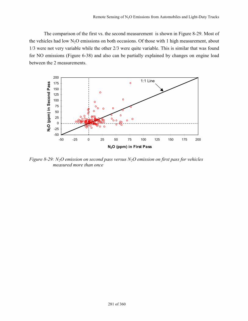
Remote Sensing of N2O Emissions from Automobiles and Light-Duty Trucks

281 of 360

The comparison of the first vs. the second measurement is shown in Figure 8-29. Most of

the vehicles had low N2O emissions on both occasions. Of those with 1 high measurement, about

1/3 were not very variable while the other 2/3 were quite variable. This is similar that was found

for NO emissions (Figure 6-38) and also can be partially explained by changes on engine load

between the 2 measurements.

-50

-25

0

25

50

75

100

125

150

175

200

-50 -25 0 25 50 75 100 125 150 175 200

N2O (ppm) in First Pass

N2O

(p

pm

) in

Sec

on

d P

ass 1:1 Line

Figure 8-29: N2O emission on second pass versus N2O emission on first pass for vehiclesmeasured more than once

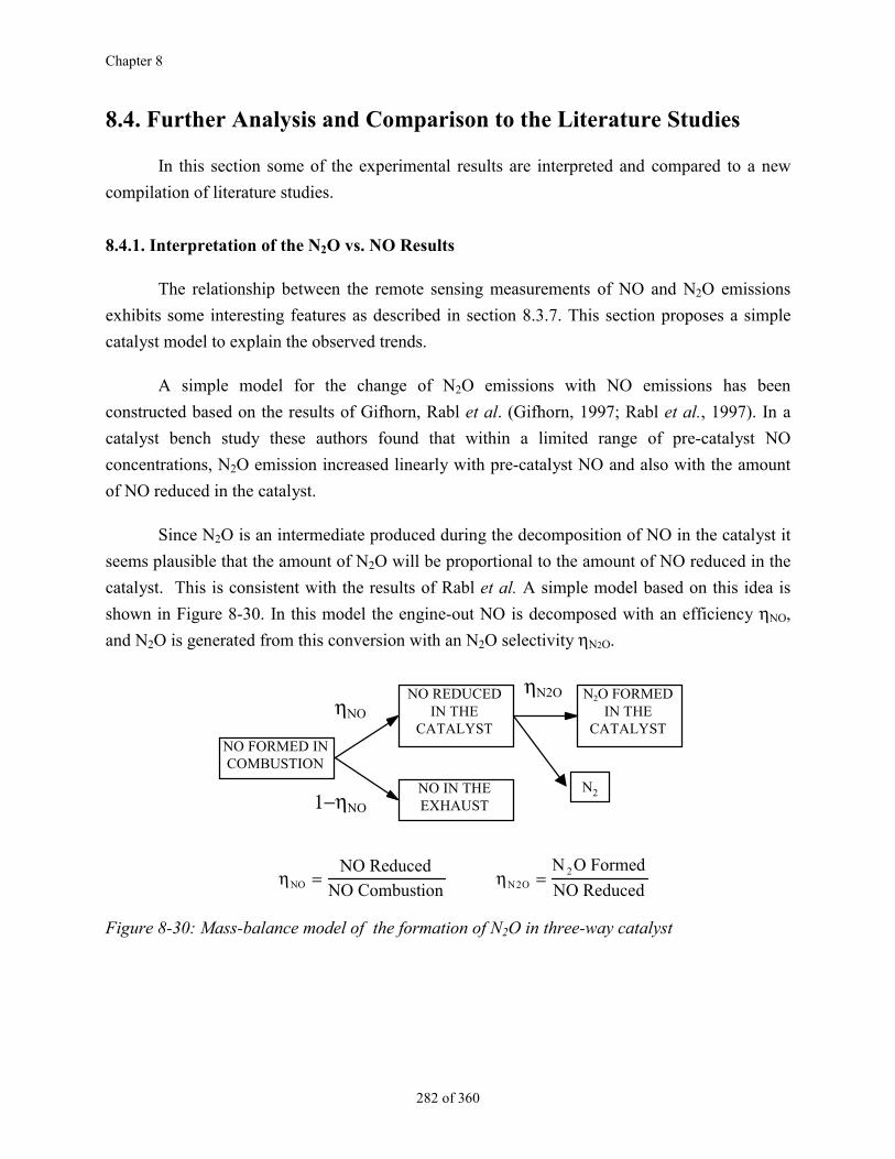
Chapter 8

282 of 360

8.4. Further Analysis and Comparison to the Literature Studies

In this section some of the experimental results are interpreted and compared to a new

compilation of literature studies.

8.4.1. Interpretation of the N2O vs. NO Results

The relationship between the remote sensing measurements of NO and N2O emissions

exhibits some interesting features as described in section 8.3.7. This section proposes a simple

catalyst model to explain the observed trends.

A simple model for the change of N2O emissions with NO emissions has been

constructed based on the results of Gifhorn, Rabl et al. (Gifhorn, 1997; Rabl et al., 1997). In a

catalyst bench study these authors found that within a limited range of pre-catalyst NO

concentrations, N2O emission increased linearly with pre-catalyst NO and also with the amount

of NO reduced in the catalyst.

Since N2O is an intermediate produced during the decomposition of NO in the catalyst it

seems plausible that the amount of N2O will be proportional to the amount of NO reduced in the

catalyst. This is consistent with the results of Rabl et al. A simple model based on this idea is

shown in Figure 8-30. In this model the engine-out NO is decomposed with an efficiency ηNO,

and N2O is generated from this conversion with an N2O selectivity ηN2O.

NO IN THEEXHAUST

NO REDUCEDIN THE

CATALYSTNO FORMED INCOMBUSTION

N2O FORMEDIN THE

CATALYSTηNO

1−ηNO

ηN2O

η ηNO N O

NO Reduced

NO Combust

N O Formed

NO Reduced= =

ion 2

2

N2

Figure 8-30: Mass-balance model of the formation of N2O in three-way catalyst

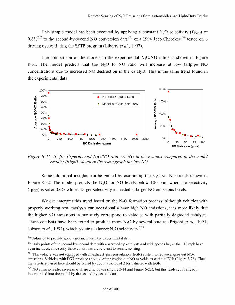
Remote Sensing of N2O Emissions from Automobiles and Light-Duty Trucks

283 of 360

This simple model has been executed by applying a constant N2O selectivity (ηN2O) of

0.6%272 to the second-by-second NO conversion data273 of a 1994 Jeep Cherokee274 tested on 8

driving cycles during the SFTP program (Liberty et al., 1997).

The comparison of the models to the experimental N2O/NO ratios is shown in Figure

8-31. The model predicts that the N2O to NO ratio will increase at low tailpipe NO

concentrations due to increased NO destruction in the catalyst. This is the same trend found in

the experimental data.

0%

25%

50%

75%

100%

125%

150%

175%

200%

0 250 500 750 1000 1250 1500 1750 2000 2250

NO Emission (ppm)

Av

era

ge

N2O

/NO

Ra

tio Remote Sensing Data

Model with S(N2O)=0.6%

0%

50%

100%

150%

200%

0 25 50 75 100NO Emission (ppm)

Ave

rag

e N

2O/N

O R

atio

Figure 8-31: (Left): Experimental N2O/NO ratio vs. NO in the exhaust compared to the modelresults; (Right): detail of the same graph for low NO

Some additional insights can be gained by examining the N2O vs. NO trends shown in

Figure 8-32. The model predicts the N2O for NO levels below 100 ppm when the selectivity

(ηN2O) is set at 0.6% while a larger selectivity is needed at larger NO emissions levels.

We can interpret this trend based on the N2O formation process: although vehicles with

properly working new catalysts can occasionally have high NO emissions, it is more likely that

the higher NO emissions in our study correspond to vehicles with partially degraded catalysts.

These catalysts have been found to produce more N2O by several studies (Prigent et al., 1991;

Jobson et al., 1994), which requires a larger N2O selectivity.275

272 Adjusted to provide good agreement with the experimental data.273 Only points of the second-by-second data with a warmed-up catalysts and with speeds larger than 10 mph havebeen included, since only those conditions are relevant to remote sensing.274 This vehicle was not equipped with an exhaust gas recirculation (EGR) system to reduce engine-out NOxemissions. Vehicles with EGR produce about ½ of the engine-out NO as vehicles without EGR (Figure 3-26). Thusthe selectivity used here should be scaled by about a factor of 2 for vehicles with EGR.275 NO emissions also increase with specific power (Figure 3-14 and Figure 6-22), but this tendency is alreadyincorporated into the model by the second-by-second data.

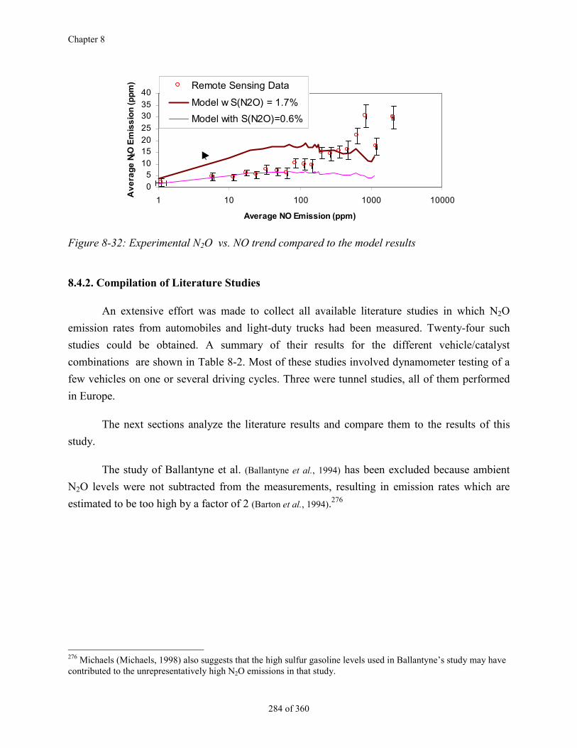
Chapter 8

284 of 360

0

510

1520

25

3035

40

1 10 100 1000 10000

Average NO Emission (ppm)

Av

era

ge

N2O

Em

iss

ion

(p

pm

) Remote Sensing Data

Model w S(N2O) = 1.7%

Model with S(N2O)=0.6%

Figure 8-32: Experimental N2O vs. NO trend compared to the model results

8.4.2. Compilation of Literature Studies

An extensive effort was made to collect all available literature studies in which N2O

emission rates from automobiles and light-duty trucks had been measured. Twenty-four such

studies could be obtained. A summary of their results for the different vehicle/catalyst

combinations are shown in Table 8-2. Most of these studies involved dynamometer testing of a

few vehicles on one or several driving cycles. Three were tunnel studies, all of them performed

in Europe.

The next sections analyze the literature results and compare them to the results of this

study.

The study of Ballantyne et al. (Ballantyne et al., 1994) has been excluded because ambient

N2O levels were not subtracted from the measurements, resulting in emission rates which are

estimated to be too high by a factor of 2 (Barton et al., 1994).276

276 Michaels (Michaels, 1998) also suggests that the high sulfur gasoline levels used in Ballantyne’s study may havecontributed to the unrepresentatively high N2O emissions in that study.

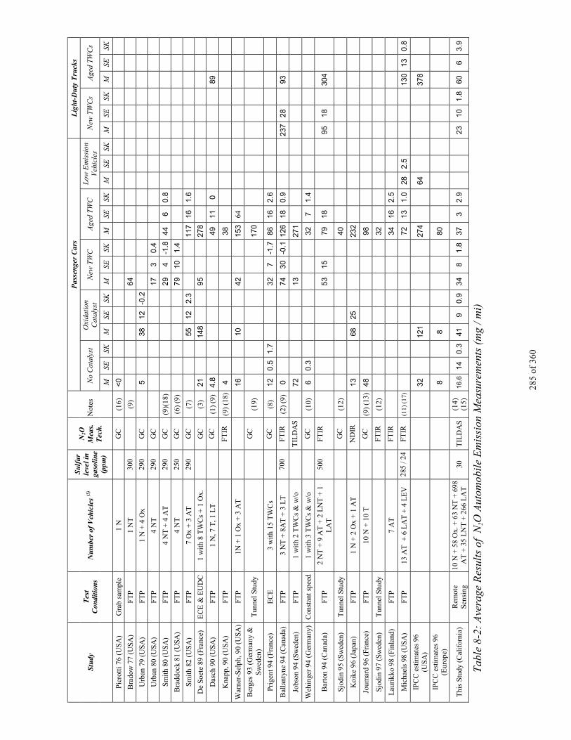
285

of 3

60

Pas

seng

er C

ars

Lig

ht-D

uty

Tru

cks

No

Cat

alys

tO

xida

tion

Cat

alys

tN

ew T

WC

Age

d TW

CL

ow E

mis

sion

Veh

icle

sN

ew T

WC

sA

ged

TWC

sS

tudy

Tes

tC

ondi

tion

sN

umbe

r of

Veh

icle

s (5

)

Su

lfu

rle

vel i

nga

soli

ne

(ppm

)

N2O

Mea

s.T

ech

.N

otes

MSE

SKM

SESK

MSE

SKM

SESK

MSE

SKM

SESK

MSE

SK

Pie

rott

i 76

(US

A)

Gra

b sa

mpl

e1

NG

C(1

6)<

0

Bra

dow

77

(US

A)

FT

P1

NT

300

(9)

64

Urb

an 7

9 (U

SA

)F

TP

1 N

+ 4

Ox

290

GC

538

12-0

.2

Urb

an 8

0 (U

SA

)F

TP

4 N

T29

0G

C17

30.

4

Sm

ith

80 (

US

A)

FT

P4

NT

+ 4

AT

290

GC

(9)(

18)

294

-1.8

446

0.8

Bra

ddoc

k 81

(U

SA

)F

TP

4 N

T25

0G

C(6

) (9

)79

101.

4

Sm

ith

82 (

US

A)

FT

P7

Ox

+ 3

AT

290

GC

(7)

5512

2.3

117

161.

6

De

Soe

te 8

9 (F

ranc

e)E

CE

& E

UD

C1

wit

h 8

TW

Cs

+ 1

Ox.

GC

(3)

2114

895

278

Das

ch 9

0 (U

SA

)F

TP

1 N

, 7 T

, 1 L

TG

C(1

) (9

)4.

849

110

89

Kna

pp, 9

0 (U

SA

)F

TP

FT

IR(9

) (1

8)4

38

War

ner-

Sel

ph, 9

0 (U

SA

)F

TP

1N +

1 O

x +

3 A

T16

1042

153

64

Ber

ges

93 (

Ger

man

y &

Sw

eden

)T

unne

l Stu

dyG

C(1

9)17

0

Pri

gent

94

(Fra

nce)

EC

E3

wit

h 15

TW

Cs

GC

(8)

120.

51.

732

7-1

.786

162.

6

Bal

lant

yne

94 (

Can

ada)

FT

P3

NT

+ 8

AT

+ 3

LT

700

FT

IR(2

) (9

)0

7430

-0.1

126

180.

923

728

93

Jobs

on 9

4 (S

wed

en)

FT

P1

wit

h 2

TW

Cs

& w

/oT

ILD

AS

7213

271

Weh

inge

r 94

(G

erm

any)

Con

stan

t spe

ed1

wit

h 3

TW

Cs

& w

/oG

C(1

0)6

0.3

327

1.4

Bar

ton

94 (

Can

ada)

FT

P2

NT

+ 9

AT

+ 2

LN

T +

1L

AT

500

FT

IR53

1579

1895

1830

4

Sjo

din

95 (

Sw

eden

)T

unne

l Stu

dyG

C(1

2)40

Koi

ke 9

6 (J

apan

)F

TP

1 N

+ 2

Ox

+ 1

AT

ND

IR13

6825

232

Joum

ard

96 (

Fran

ce)

FT

P10

N +

10

TG

C(9

) (1

3)48

98

Sjo

din

97 (

Sw

eden

)T

unne

l Stu

dyF

TIR

(12)

32

Lau

rikk

o 98

(Fi

nlan

d)F

TP

7 A

TF

TIR

3416

2.5

Mic

hael

s 98

(U

SA

)F

TP

13 A

T +

6 L

AT

+ 4

LE

V28

5 / 2

4F

TIR

(11)

(17

)72

131.

028

2.5

130

130.

8

IPC

C e

stim

ates

96

(US

A)

3212

127

464

378

IPC

C e

stim

ates

96

(Eur

ope)

88

80

Thi

s S

tudy

(C

alif

orni

a)R

emot

eS

ensi

ng10

N +

58

Ox.

+ 6

3 N

T +

698

AT

+ 3

5 L

NT

+ 2

66 L

AT

30T

ILD

AS

(14)

(15)

16.6

140.

341

90.

934

81.

837

32.

923

101.

860

63.

9

Tab

le 8

-2:

Ave

rage

Res

ults

of

N2O

Aut

omob

ile

Em

issi

on M

easu

rem

ents

(m

g / m

i)

286 of 360

Notes for Table 8-2

Key: M: mean; SE: Standard Error of the Mean; SK: Skewness

(1): No distinction was made between new and aged catalysts in Dasch’ study, and the mileage of the testedvehicles was not provided. Dasch averaged his results with those of previous studies, but only themeasurements performed during his study have been included here.(2): The N2O detection limit is not reported. I estimate it at about 360 ppb based on the reported results.The ambient N2O level was not subtracted from the measurements. For this reason this study has not beenincluded in the average of the literature.(3): Only the data for which the subtraction of the ambient N2O concentration from the bag samples wasperformed systematically have been included (table XXIX of this report, line 2).(5): N: non-catalyst; Ox: Oxidation Catalyst; T: three-way catalyst; NT: New Three-Way Catalyst; AT:Aged Three-Way Catalyst; L: Low Emission Vehicle; LT: light-duty truck with three-way catalyst(6): The vehicles were new with conditioning “by on road mileage accumulation.” The conditioningmileage is not reported. These vehicles have been included in the “new three-way catalyst” category(7): This study tested the vehicles “as received” and after a tune-up. Only the “as received” data are usedhere since they are more representative of real-world emissions(8): Catalysts aged 50, 100, and 150 hours have been combined into the “aged catalyst” group in this table.(9): These studies included data on driving cycles other than the FTP, which are not presented in this table.Some of these results have been presented in section 8.2.(10): Results are reported in ppm. The conversion to mg/mi assumed a fuel economy of 10L/100km(Berges 1993). All three catalysts with 16,000-95,000 miles have been grouped under “aged catalysts” here(11): Averages of all data for both air conditioning modes. Results with standard sulfur content presentedhere for all vehicles except Low Emission Vehicles; low-S fuel results presented for the later(12): These results correspond to a mixed vehicle fleet of about 45% TWC passenger cars, 45% non-catalyst cars, and 10% heavy-duty vehicles(13): No mileage reported for the TWC vehicles; all have been included in the “aged catalyst” category(14): No independent measurement for the non-catalyst vehicles since this value was used to correct theaverage systematic bias of the data set (Appendix E).(15): Total number of vehicles is smaller than the 1361 vehicles sampled because license plates were notcaptured for 10% of the vehicles, the California Department of Motor Vehicles could not provideregistration information for about 10% of the license plates captured, and the VIN decoder could notdecode about 10% of the VINs from the DMV.(16): The results of this study are reported in more detail in Dasch (1992) than in the original paper.(17): This study makes a further distinction between the three way catalyst-equipped vehicles subject to“Tier 0” and “Tier 1” US emission standards. This distinction has been used in the calculation of emissionfactors in section 8.5.1 but is not presented on this table.(18): This publication did not provide data for all the FTP tests included on their averages. The author wascontacted and was not able to provide those data either.(19): This study tested 4 vehicles new and after three 5,000-miles accumulation periods. The results of thenew vehicles have been included on the “new” catalyst category and those at the end of the 3rd

accumulation period on the “aged” catalyst category. The results of the intermediate accumulation periodshave not been used here.(20): This study estimated the emission rate from the N2O/CO2 ratio by extrapolating the emission to globalconditions by using global gasoline consumption, and then dividing by a global estimate of vehicle-milestraveled. This procedure may have introduced significant errors in the result.

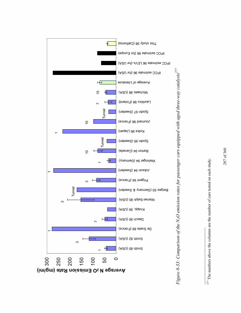
287

of 3

60

0

50

10

0

15

0

20

0

25

0

30

0

Smith 80 (USA)

Smith 82 (USA)

De Soete 89 (France)

Dasch 90 (USA)

Knapp, 90 (USA)

Warner-Selph 90 (USA)

Berges 93 (Germany & Sweden)

Prigent 94 (France)

Jobson 94 (Sweden)

Wehinger 94 (Germany)

Barton 94 (Canada)

Sjodin 95 (Sweden)

Koike 96 (Japan)

Joumard 96 (France)

Sjodin 97 (Sweden)

Laurikko 98 (Finland)

Michaels 98 (USA)

Average of Literature

IPCC estimate 96 (for USA)

IPCC estimate 96 LEVs (for USA)

IPCC estimate 96 (for Europe)

This study 98 (California)

Average N 2O Emission Rate (mg/mi)

17

1

3Tu

nnel

3

1

310

Tunn

el

10

1

1

Tunn

el

715

Fig

ure

8-33

: C

ompa

riso

n of

the

N2O

em

issi

on r

ates

for

pass

enge

r ca

rs e

quip

ped

wit

h ag

ed th

ree-

way

cat

alys

ts27

7

277 T

he n

umbe

rs a

bove

the

colu

mns

are

the

num

ber

of c

ars

test

ed o

n ea

ch s

tudy

.

Chapter 8

288 of 360

8.4.3. Comparison of the Literature Studies

A comparison of the emission rates for three-way catalyst equipped passenger

cars in the literature is shown in Figure 8-33. The range of emission rates reported in the

different studies span an order of magnitude, without a clear trend with time, location of

the study, or analysis technique.278

This large variability can be explained, however by the skewness of the N2O

emissions distribution, this is, the fact that the N2O distribution is composed of a few

super-emitters and a large majority of low-emitters (section 8.3.2). Given that most of the

studies only tested a few vehicles, the presence or absence of high emitters in the sample

can result in high or low emission rates. In particular, the three studies with the highest

emission rates only involved 1 vehicle.

The study by De Soete (De Soete, 1989), was basically adopted as the 1996 IPCC

emission factor for the U.S. (IPCC, 1996b; Michaels, 1998), which explains why this

factor was so high: it is based on the measurements on a single vehicle and several non-

production catalysts with high emitting characteristics. All of the studies in which larger

samples were used yielded significantly lower results.

Just the opposite happened in the study of Dasch at General Motors Research

Labs (Dasch, 1992). This researcher tested several vehicles with (possibly) new

catalysts279 (thus lower N2O emitters). Dasch also rejected two high emitters as outliers

with an statistical criterion which was not appropriate for highly skewed distributions.

This issue is further explored in the next section by analyzing the emissions

distribution of the literature studies.

8.4.4. Further Evidence of the Skewness of the N2O Distribution

The remote sensing study reported here has found evidence of the skewness of the

N2O emission distribution. In order to further verify this point, the distribution of N2O

278 A large positive bias in the measurement of N2O from combustion sources was found for studies usinggas chromatography due to a sampling artifact (Muzio et al., 1989). However this problem was found to beinsignificant when the SO2 concentration in the combustion gases was lower than 500 ppm (Muzio et al.,1989), which is about two orders of magnitude larger than in diluted gasoline-powered vehicle exhaust.279 The mileage of the vehicles tested in not reported in Dasch’ study.

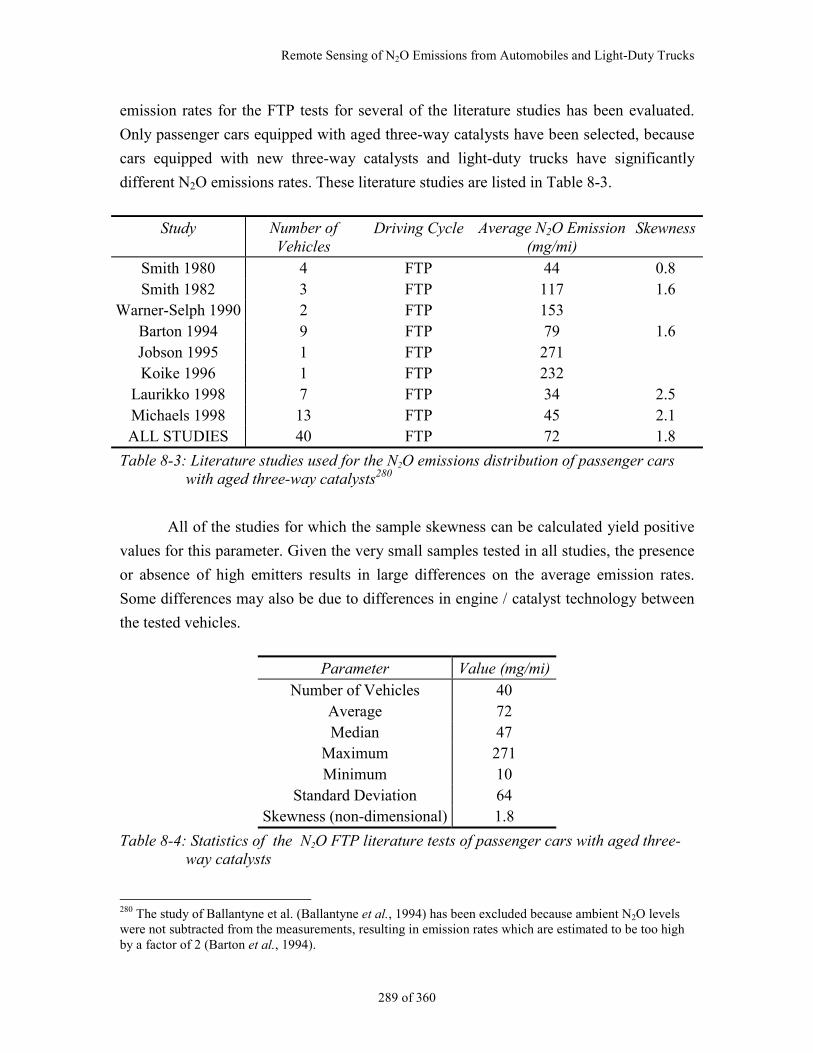
Remote Sensing of N2O Emissions from Automobiles and Light-Duty Trucks

289 of 360

emission rates for the FTP tests for several of the literature studies has been evaluated.

Only passenger cars equipped with aged three-way catalysts have been selected, because

cars equipped with new three-way catalysts and light-duty trucks have significantly

different N2O emissions rates. These literature studies are listed in Table 8-3.

Study Number ofVehicles

Driving Cycle Average N2O Emission(mg/mi)

Skewness

Smith 1980 4 FTP 44 0.8Smith 1982 3 FTP 117 1.6

Warner-Selph 1990 2 FTP 153Barton 1994 9 FTP 79 1.6Jobson 1995 1 FTP 271Koike 1996 1 FTP 232

Laurikko 1998 7 FTP 34 2.5Michaels 1998 13 FTP 45 2.1ALL STUDIES 40 FTP 72 1.8

Table 8-3: Literature studies used for the N2O emissions distribution of passenger carswith aged three-way catalysts280

All of the studies for which the sample skewness can be calculated yield positive

values for this parameter. Given the very small samples tested in all studies, the presence

or absence of high emitters results in large differences on the average emission rates.

Some differences may also be due to differences in engine / catalyst technology between

the tested vehicles.

Parameter Value (mg/mi)Number of Vehicles 40

Average 72Median 47

Maximum 271Minimum 10

Standard Deviation 64Skewness (non-dimensional) 1.8

Table 8-4: Statistics of the N2O FTP literature tests of passenger cars with aged three-way catalysts

280 The study of Ballantyne et al. (Ballantyne et al., 1994) has been excluded because ambient N2O levelswere not subtracted from the measurements, resulting in emission rates which are estimated to be too highby a factor of 2 (Barton et al., 1994).

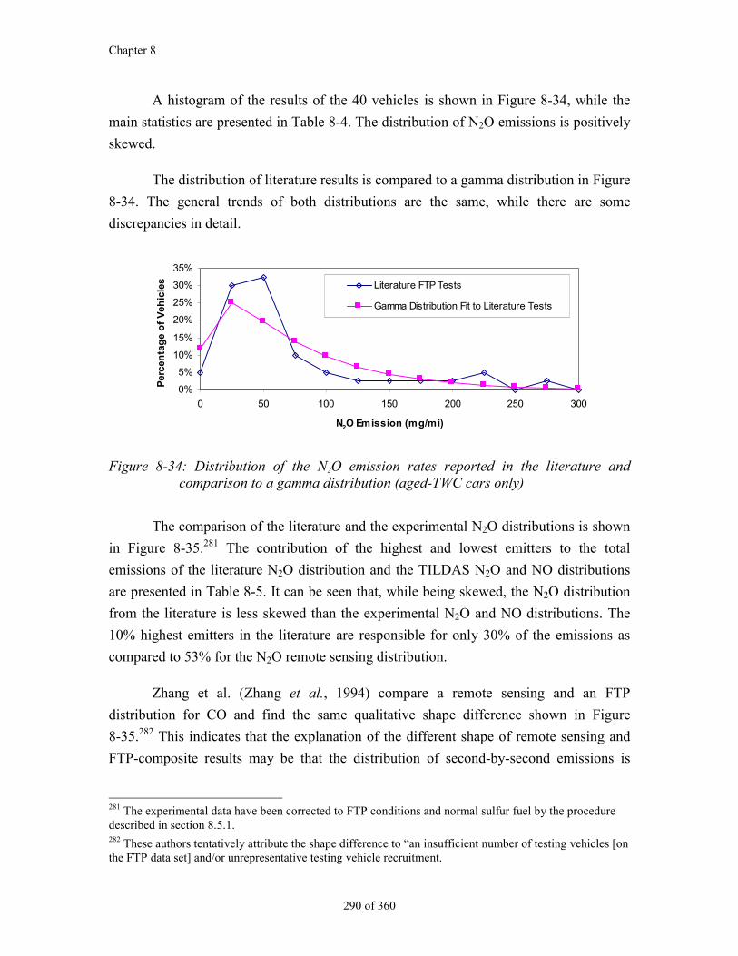
Chapter 8

290 of 360

A histogram of the results of the 40 vehicles is shown in Figure 8-34, while the

main statistics are presented in Table 8-4. The distribution of N2O emissions is positively

skewed.

The distribution of literature results is compared to a gamma distribution in Figure

8-34. The general trends of both distributions are the same, while there are some

discrepancies in detail.

0%

5%

10%

15%

20%

25%

30%

35%

0 50 100 150 200 250 300

N2O Emission (mg/mi)

Per

cen

tag

e o

f V

ehic

les Literature FTP Tests

Gamma Distribution Fit to Literature Tests

Figure 8-34: Distribution of the N2O emission rates reported in the literature andcomparison to a gamma distribution (aged-TWC cars only)

The comparison of the literature and the experimental N2O distributions is shown

in Figure 8-35.281 The contribution of the highest and lowest emitters to the total

emissions of the literature N2O distribution and the TILDAS N2O and NO distributions

are presented in Table 8-5. It can be seen that, while being skewed, the N2O distribution

from the literature is less skewed than the experimental N2O and NO distributions. The

10% highest emitters in the literature are responsible for only 30% of the emissions as

compared to 53% for the N2O remote sensing distribution.

Zhang et al. (Zhang et al., 1994) compare a remote sensing and an FTP

distribution for CO and find the same qualitative shape difference shown in Figure

8-35.282 This indicates that the explanation of the different shape of remote sensing and

FTP-composite results may be that the distribution of second-by-second emissions is

281 The experimental data have been corrected to FTP conditions and normal sulfur fuel by the proceduredescribed in section 8.5.1.282 These authors tentatively attribute the shape difference to “an insufficient number of testing vehicles [onthe FTP data set] and/or unrepresentative testing vehicle recruitment.

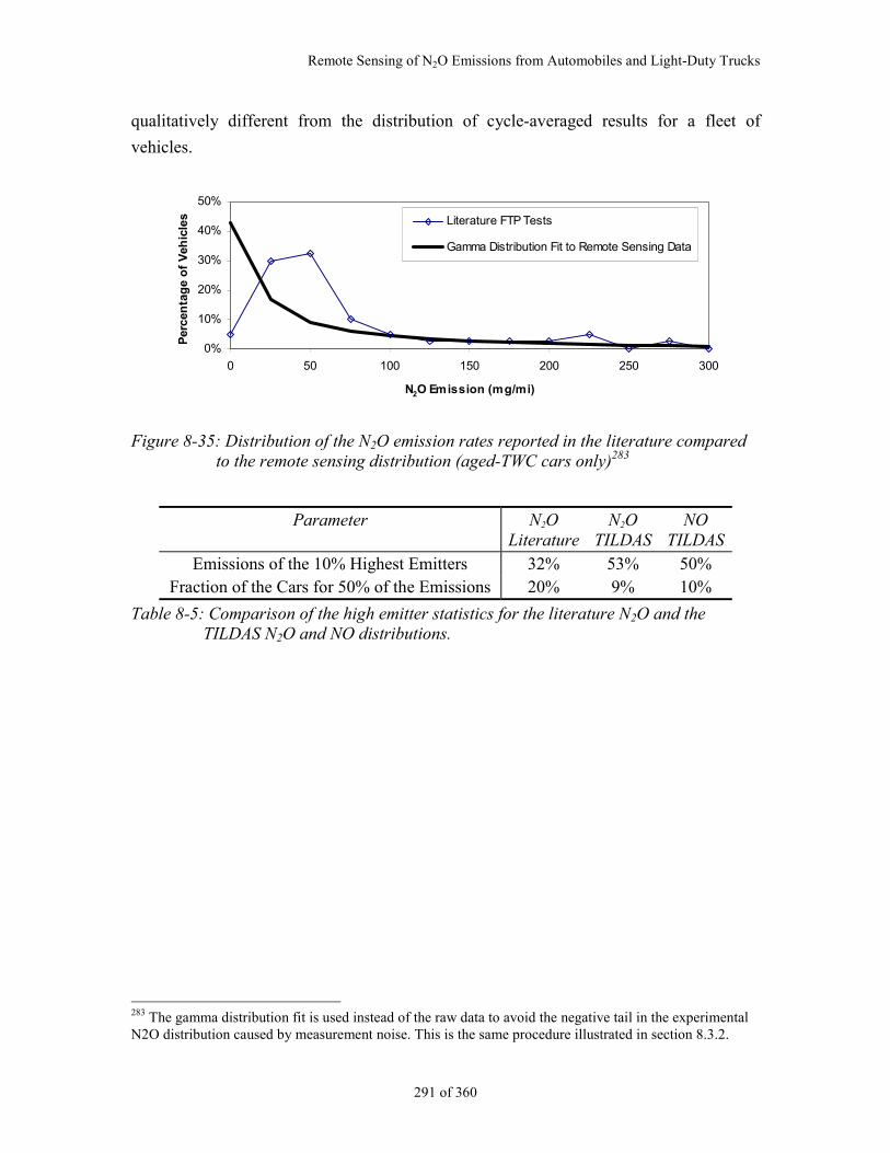
Remote Sensing of N2O Emissions from Automobiles and Light-Duty Trucks

291 of 360

qualitatively different from the distribution of cycle-averaged results for a fleet of

vehicles.

0%

10%

20%

30%

40%

50%

0 50 100 150 200 250 300

N2O Emission (mg/mi)

Per

cen

tag

e o

f V

ehic

les Literature FTP Tests

Gamma Distribution Fit to Remote Sensing Data

Figure 8-35: Distribution of the N2O emission rates reported in the literature comparedto the remote sensing distribution (aged-TWC cars only)283

Parameter N2OLiterature

N2OTILDAS

NOTILDAS

Emissions of the 10% Highest Emitters 32% 53% 50%Fraction of the Cars for 50% of the Emissions 20% 9% 10%

Table 8-5: Comparison of the high emitter statistics for the literature N2O and theTILDAS N2O and NO distributions.

283 The gamma distribution fit is used instead of the raw data to avoid the negative tail in the experimentalN2O distribution caused by measurement noise. This is the same procedure illustrated in section 8.3.2.

Chapter 8

292 of 360

8.5. N2O Emission Factors

8.5.1. N2O Emission Factor Estimation from TILDAS Remote Sensing Data

The estimation of real-world N2O emission factors from passenger cars and light-

duty trucks is of great interest due to the large uncertainties that remain about their value

(Michaels, 1998). We have shown that remote sensing can produce emission factors for

NOx for light-duty vehicles and heavy-duty diesel trucks which are close to those

determined in several tunnel studies (see Figure 6-15 and Figure 7-13). Also we have

shown in section 8.2 that remote sensing is well suited for estimating emission factors for

N2O emissions. This section details the calculation procedure and the results based on the

N2O remote sensing data collected in California.

The emission factors for this study were determined separately for each catalyst

vehicle type and technology. The remote sensing emission factor for each technology

group has been estimated in the following way:

The average N2O emission (ppm) of every model year passenger cars and light-duty

trucks has been calculated separately from the experimental data.

The average N2O emission rate (mg/mi) has been calculated using the fuel economy

of each vehicle type and model year.

The emission factor for passenger cars, light-duty trucks, and all vehicles has been

computed as the average of the emission rates of every model year and vehicle type,

weighed by the number of vehicles in each year and type.

This procedure results in an estimate of the N2O emission factors that each type of

vehicle was actually emitting at our remote sensing site. In order to make the remote

sensing results comparable with the literature results and IPCC / EPA estimates which

have mostly used the FTP cycle and high sulfur gasoline, some factors need to be

corrected for:

First we have to account for the fact that although we measured warm-running

emissions at our remote sensing site, the vehicles were not exactly on average at the

same conditions as during the FTP Bag 2. Vehicle emissions have been shown to be

closely related to vehicle specific power in Chapter 3. Average specific power in our

study was larger than the average specific power in Bag 2 of the FTP. The emission

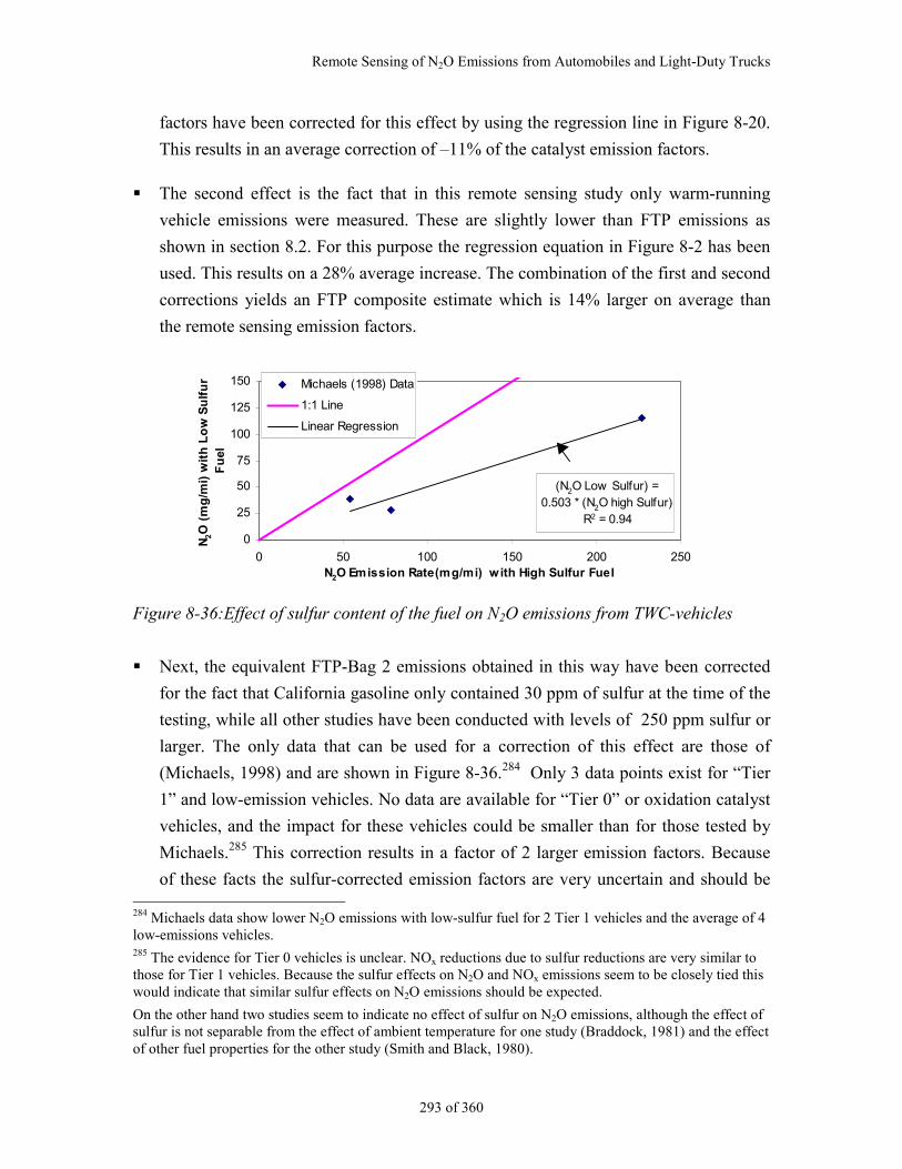
Remote Sensing of N2O Emissions from Automobiles and Light-Duty Trucks

293 of 360

factors have been corrected for this effect by using the regression line in Figure 8-20.

This results in an average correction of –11% of the catalyst emission factors.

The second effect is the fact that in this remote sensing study only warm-running

vehicle emissions were measured. These are slightly lower than FTP emissions as

shown in section 8.2. For this purpose the regression equation in Figure 8-2 has been

used. This results on a 28% average increase. The combination of the first and second

corrections yields an FTP composite estimate which is 14% larger on average than

the remote sensing emission factors.

(N2O Low Sulfur) = 0.503 * (N2O high Sulfur)

R2 = 0.94

0

25

50

75

100

125

150

0 50 100 150 200 250N2O Emission Rate(mg/mi) with High Sulfur Fuel

N2O

(m

g/m

i) w

ith

Lo

w S

ulf

ur

Fu

el

Michaels (1998) Data

1:1 Line

Linear Regression

Figure 8-36:Effect of sulfur content of the fuel on N2O emissions from TWC-vehicles

Next, the equivalent FTP-Bag 2 emissions obtained in this way have been corrected

for the fact that California gasoline only contained 30 ppm of sulfur at the time of the

testing, while all other studies have been conducted with levels of 250 ppm sulfur or

larger. The only data that can be used for a correction of this effect are those of

(Michaels, 1998) and are shown in Figure 8-36.284 Only 3 data points exist for “Tier

1” and low-emission vehicles. No data are available for “Tier 0” or oxidation catalyst

vehicles, and the impact for these vehicles could be smaller than for those tested by

Michaels.285 This correction results in a factor of 2 larger emission factors. Because

of these facts the sulfur-corrected emission factors are very uncertain and should be 284 Michaels data show lower N2O emissions with low-sulfur fuel for 2 Tier 1 vehicles and the average of 4low-emissions vehicles.285 The evidence for Tier 0 vehicles is unclear. NOx reductions due to sulfur reductions are very similar tothose for Tier 1 vehicles. Because the sulfur effects on N2O and NOx emissions seem to be closely tied thiswould indicate that similar sulfur effects on N2O emissions should be expected.

On the other hand two studies seem to indicate no effect of sulfur on N2O emissions, although the effect ofsulfur is not separable from the effect of ambient temperature for one study (Braddock, 1981) and the effectof other fuel properties for the other study (Smith and Black, 1980).

Chapter 8

294 of 360

taken as tentative, while the factors without the sulfur correction can be taken as

lower limits.

Previous inventories account for all U.S. vehicle-miles-traveled (VMT) with

N2O emission factors derived on the FTP. This ignores the fact that a

significant part of the VMT is accumulated on highways, where N2O

emissions tend to be lower due to higher catalyst temperatures. Highway

emission factors have been estimated here by applying the regression equation

of the HWFET to the FTP driving cycle emissions (Figure 8-4)286 to the

emission factors determined in this study.

8.5.2. Comparison to the Literature and IPCC / EPA N2O Emission Factors

The results of this study are compared to the latest IPCC and EPA estimates

(IPCC, 1996b; U.S. EPA, 1997b; Michaels, 1998) and to the averages of the literature

values in Table 8-6. The averages of the literature values have been calculated from the

results from 23 literature studies in which N2O emission rates of on-road vehicles were

measured are reported in Table 8-2. Most of the studies involved a testing one or few

vehicles in a chassis dynamometer, and 3 were tunnel studies.

286 Differences in Specific Power distributions between the two cycles may not be as important as for otherpollutants, since N2O emissions are not highly sensitive to Specific Power (Figure 8-20).

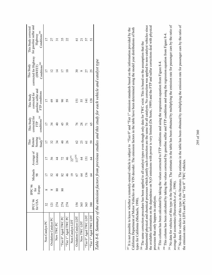
295

of 3

60

IPC

C 9

6fo

r U

SA

IPP

C 9

6fo

rE

urop

e

Mic

hael

s98

Ave

rage

of

Lit

erat

ure

Thi

sR

emot

eS

ensi

ng

Stu

dy28

7

Thi

s S

tudy

corr

ecte

d fo

rF

TP

cond

itio

ns28

8

Thi

s S

tudy

corr

ecte

d fo

rga

soli

ne s

ulfu

r an

dF

TP

con

diti

ons

Thi

s S

tudy

corr

rect

ed f

or H

ighw

ay(H

WF

ET

)

Con

diti

ons28

9

Thi

s S

tudy

cor

rect

edfo

r ga

soli

ne s

ulfu

r an

dH

ighw

ay

Con

diti

ons29

0

Non

-Cat

alys

t PC

328

1717

1717

1717

17

Oxi

dati

on C

atal

yst P

C12

18

5256

3234

6912

27

New

TW

C P

C27

480

4644

3440

8014

31

“Tie

r 0”

Age

d T

WC

PC

274

8082

7240

4590

1735

“Tie

r 1”

Age

d T

WC

PC

274

4646

2630

5910

22

Non

-Cat

alys

t LD

T19

2229

1

Oxi

dati

on C

atal

yst L

DT

156

6711

7292

6276

151

3061

New

TW

C L

DT

365

6464

2328

559

21

“Tie

r 0”

Age

d T

WC

LD

T36

513

615

161

7114

127

57

“Tie

r 1”

Age

d T

WC

LD

T38

064

6459

6512

825

51

Tab

le 8

-6:

Sum

mar

y of

the

emis

sion

fact

ors

from

pre

viou

s st

udie

s an

d th

is s

tudy

for

each

veh

icle

and

cat

alys

t typ

e

287 I

t is

not p

ossi

ble

to k

now

whe

ther

a r

emot

ely-

sens

ed v

ehic

le is

sub

ject

to “

Tie

r 0”

and

“T

ier

1” e

mis

sion

sta

ndar

ds b

ased

on

the

info

rmat

ion

prov

ided

by

the

Cal

ifor

nia

Dep

artm

ent o

f M

otor

Veh

icle

s or

the

VIN

dec

oder

. The

em

issi

on f

acto

rs in

the

tabl

e ha

ve b

een

dete

rmin

ed u

sing

the

mod

el y

ear

dist

ribu

tion

s of

bot

hty

pes

for

Cal

ifor

nia

(Mic

hael

s, 1

998)

.28

8 The

sam

e co

rrec

tion

pro

cedu

re h

as b

een

appl

ied

to a

ll c

atal

yst t

ypes

eve

n th

ough

onl

y da

ta f

or T

WC

exi

st. T

his

is b

ased

on

the

assu

mpt

ion

that

the

fund

amen

tal p

hysi

cal a

nd c

hem

ical

pro

cess

es w

hich

just

ify

each

cor

rect

ion

are

the

sam

e fo

r al

l cat

alys

ts. N

o co

rrec

tion

was

app

lied

to n

on-c

atal

yst v

ehic

les

sinc

eth

e av

aila

ble

info

rmat

ion

on th

e de

pend

ence

on

N2O

em

issi

ons

wit

h po

wer

is v

ery

lim

ited

(D

e S

oete

, 198

9) a

nd th

e F

TP

and

sul

fur

corr

ecti

ons

deal

wit

h ph

ysic

alpr

oces

ses

that

onl

y ha

ppen

in c

atal

ysts

.28

9 Thi

s co

lum

n ha

s be

en c

alcu

late

d by

taki

ng th

e va

lues

cor

rect

ed to

FT

P c

ondi

tion

s an

d us

ing

the

regr

essi

on e

quat

ion

from

Fig

ure

8-4.

290 T

his

colu

mn

has

been

cal

cula

ted

by ta

king

the

valu

es c

orre

cted

by

gaso

line

sul

fur

and

FT

P c

ondi

tion

s an

d us

ing

the

regr

essi

on e

quat

ion

from

Fig

ure

8-4.

291 N

o da

ta f

or v

ehic

les

of th

is ty

pe in

the

lite

ratu

re. T

he e

stim

ate

in th

e ta

ble

has

been

obt

aine

d by

mul

tipl

ying

the

emis

sion

rat

e fo

r pa

ssen

ger

cars

by

the

rati

o of

aver

age

fuel

eco

nom

ies

(Hea

venr

ich

et a

l., 1

996)

.29

2 No

data

for

veh

icle

s of

this

type

in th

e li

tera

ture

. The

est

imat

e in

the

tabl

e ha

s be

en o

btai

ned

by m

ulti

plyi

ng th

e em

issi

on r

ate

for

pass

enge

r ca

rs b

y th

e ra

tio

ofth

e em

issi

on r

ates

for

LD

Ts

and

PC

s fo

r “T

ier

0” T

WC

veh

icle

s.

Chapter 8

296 of 360

These comparisons are also shown in Figure 8-37 and Figure 8-38. The main

conclusions of the comparison between the average literature values and the results of

this study (Figure 8-38) are:293

The results of this remote sensing study are lower than the average of the literature

values for all the vehicle/catalyst combinations. Once corrected to FTP conditions and

normal sulfur gasoline, the results of this study are slightly higher for all the

passenger car types. These differences are not highly significant, given the

uncertainties in this study294 and in the correction for the gasoline sulfur content.

For light-duty trucks the uncorrected results are about ½ of the literature values for

new catalysts and “Tier 0” TWC vehicles, and about the same for “Tier 1” TWC

vehicles.

The light-duty truck results corrected to FTP conditions and normal gasoline sulfur

levels are very close to the average of the literature for new catalysts and “Tier 0”

TWC vehicles.

The corrected remote sensing result is twice as large for “Tier 1” TWC LDTs than for

the literature.295 This is important since this vehicle type accounted for 10% of the

vehicle-miles traveled (VMT) in the U.S. in 1996 (U.S. EPA, 1998i) and will be

increasing as all new light-duty trucks are subject to this or stricter standards.

LDTs equipped with oxidation catalysts have the largest emission rate of the remote

sensing study.296 This result is highly uncertain due to the small number of vehicles in

this category (14). No N2O measurements on vehicles of this type have been reported

in the literature, so a comparison is not possible. Again a larger vehicle sample would

be needed to get a more precise estimate. This point is not too important because this

vehicle type accumulated only 5% of the VMT (U.S. DOT, 1997a), and this share 293 Non-catalyst emission factors are discussed in Appendix E.294 Due to the uncertainty in the correction of the negative bias (Appendix E).295 This difference would be about slightly less if the “new catalyst” LDTs (which are subject to Tier 1 orstricter standards) 295 and “Tier 1” TWC vehicle categories were combined. This may or may not be fair,since the lower emissions of the “new catalyst” category could be due to lack of catalyst aging. A largersample than the one in this study would be needed to ascertain this point.296 This emission rate is similar to that of the LDTs equipped with aged TWCs. The emission rate ofpassenger cars equipped with oxidation catalyst is also similar to the levels from TWC-equipped cars,which indicates that this result is plausible.

Remote Sensing of N2O Emissions from Automobiles and Light-Duty Trucks

297 of 360

will be declining with time as oxidation catalysts are no longer used by themselves in

automotive applications (Michaels 1998).

Estimated highway emission rates are only 42% of the FTP emission rates. This fact

has an important impact on the estimates of the total U.S. N2O mobile source

emissions.

The conclusions of the comparison between the IPCC 96 / EPA 98 estimates, the

average literature values, and the results of this study (Figure 8-38) are:

The average literature values for catalyst vehicles are within ±15% of the newest

EPA emission factors proposed by Michaels (Michaels, 1998).297 The raw remote

sensing results are generally lower than EPA’s new factors and the sulfur-corrected

numbers are higher.

The IPCC 96 / Draft EPA 98 N2O emission factors (IPCC, 1996b; U.S. EPA, 1998c)

that originated from the report of Weaver and Chan (Weaver and Chan, 1996) are a

factor of 3-5 higher than the average literature values and the corrected results of this

study, and about a factor of 7 higher than the uncorrected remote sensing results. The

main reason for this discrepancy (as pointed out by Michaels (Michaels, 1998)) is that

the emission factors of Weaver and Chan are based mostly on the results of De Soete

(De Soete, 1989),298 which are much higher than the average literature results. De

Soete tested only 1 vehicle with several three-way catalysts. The vehicle-catalysts

combinations tested had high emissions, but not higher than the higher emitters tested

by other researchers. The key point is that the N2O emissions distribution is very

skewed (see sections 8.3.2, 8.4.4, and 8.4.3) and De Soete happened to test a set of

mostly high emitting vehicle-catalyst combinations.

The European emission factors in the IPCC 96 guidelines (IPCC, 1996b) for aged-

TWC passenger cars are very close to the average of the literature and the results of

this study.

297 The “Tier 1” emission factors are the same as those of Michaels since his study is the only one that hasmeasured N2O emission rates from this type of vehicles.298 Actually Weaver and Chan took their numbers from a table on Ballantyne et al. (Ballantyne et al.,1994), which cited De Soete’s data (Michaels, 1998). Ballantyne’s own data were too high by a factor of 2because ambient N2O levels had not been substracted (Barton et al., 1994) from the analysis and maybe thehigh sulfur in the test gasoline (Michaels, 1998). This fact probably made the very high emission factorsfrom De Soete appear “within the range” of plausible values.

Chapter 8

298 of 360

The European emission factor for oxidation catalysts is a factor of 5-10 too low. This

discrepancy may not be important since oxidation catalysts are not very common in

Europe.

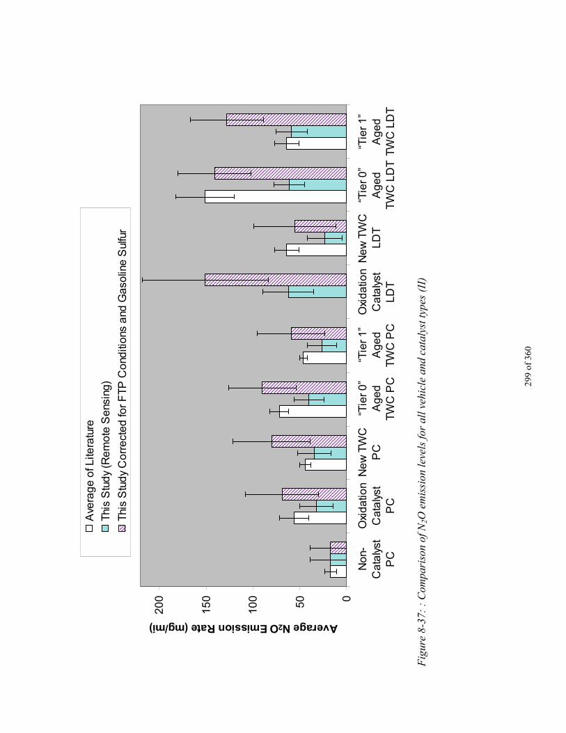
299

of 3

60����������������������

������������������������������������������������������������������������������

��������������������������������������������������������������������������������������

������������������������������������������������������������������������������������������������������

���������������������������������������������������������������������������������������������������������

���������������������������������������������������������������������������������������������������������������������������������������������������������������������������������������������������������������������������������������������������������

���������������������������������������������������������������������������������������������

���������������������������������������������������������������������������������������������������������������������������������������������������������������������������������������������������������������������������������

���������������������������������������������������������������������������������������������������������������������������������������������������������������������������������������������������������������������

0

50

10

0

15

0

20

0

No

n-C

ata

lyst

PC

Oxi

da

tion

Ca

taly

stP

C

Ne

w T

WC

PC

“Tie

r 0

”A

ge

dT

WC

PC

“Tie

r 1

”A

ge

dT

WC

PC

Oxi

da

tion

Ca

taly

stL

DT

Ne

w T

WC

LD

T“T

ier

0”

Ag

ed

TW

C L

DT

“Tie

r 1

”A

ge

dT

WC

LD

T

Average N2O Emission Rate (mg/mi)A

vera

ge

of L

itera

ture

Thi

s S

tud

y (R

em

ote

Se

nsin

g)

��������������

Thi

s S

tud

y C

orr

ect

ed

for

FT

P C

ond

itio

ns a

nd G

aso

line

Sul

fur

Fig

ure

8-37

: :

Com

pari

son

of N

2O e

mis

sion

leve

ls fo

r al

l veh

icle

and

cat

alys

t typ

es (

II)

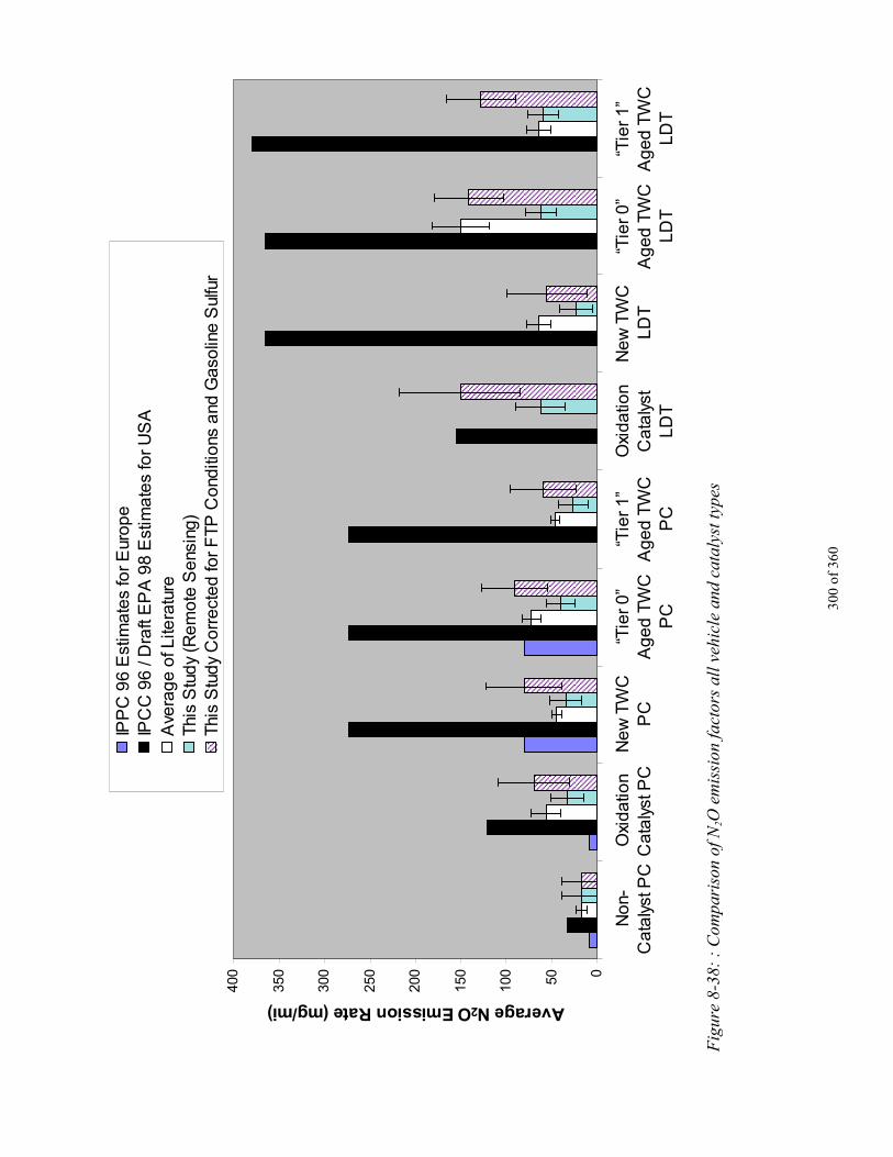
300

of 3

60

������������������

��������������������������������������������������

����������������������������������������������������������

������������������������������������������������������������������

������������������������������������������

��������������������������������������������������������������������������������������������������

������������������������������������������

��������������������������������������������������������������������������������������������������

������������������������������������������������������������������������������������������

050100

150

200

250

300

350

400

No

n-C

ata

lyst

PC

Oxi

da

tion

Ca

taly

st P

CN

ew

TW

CP

C“T

ier

0”

Ag

ed

TW

CP

C

“Tie

r 1

”A

ge

d T

WC

PC

Oxi

da

tion

Ca

taly

stL

DT

Ne

w T

WC

LD

T“T

ier

0”

Ag

ed

TW

CL

DT

“Tie

r 1

”A

ge

d T

WC

LD

T

Average N2O Emission Rate (mg/mi)IP

PC

96

Est

ima

tes

for

Eur

op

eIP

CC

96

/ D

raft

EP

A 9

8 E

stim

ate

s fo

r U

SA

Ave

rag

e o

f Lite

ratu

reT

his

Stu

dy

(Re

mo

te S

ens

ing

)

������Thi

s S

tud

y C

orr

ect

ed

for

FT

P C

ond

itio

ns a

nd G

aso

line

Sul

fur

Fig

ure

8-38

: :

Com

pari

son

of N

2O e

mis

sion

fact

ors

all v

ehic

le a

nd c

atal

yst t

ypes

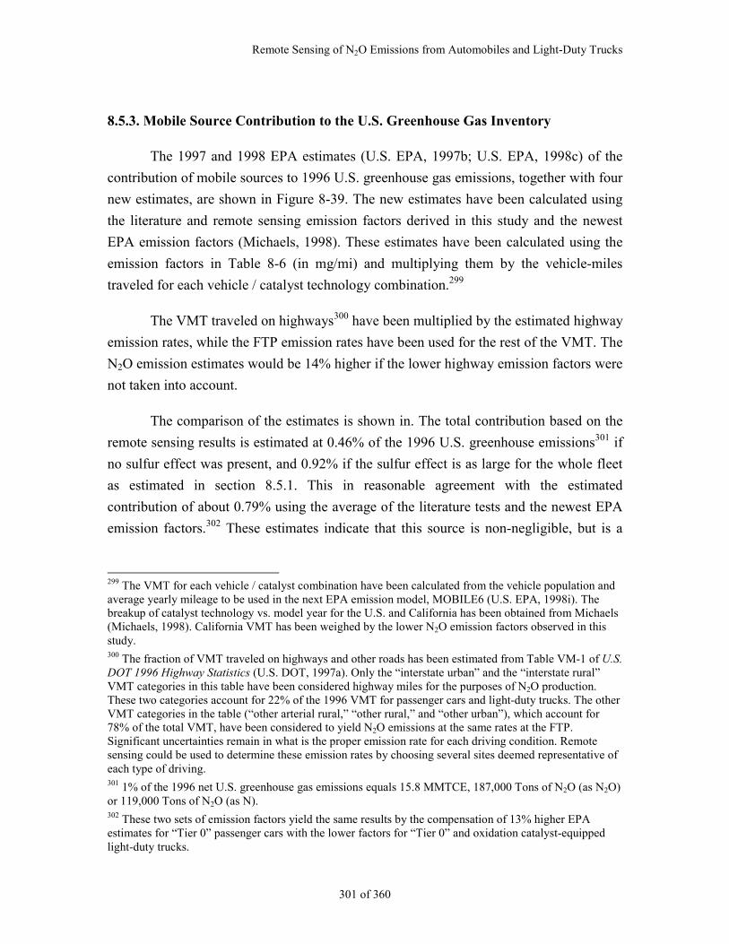
Remote Sensing of N2O Emissions from Automobiles and Light-Duty Trucks

301 of 360

8.5.3. Mobile Source Contribution to the U.S. Greenhouse Gas Inventory

The 1997 and 1998 EPA estimates (U.S. EPA, 1997b; U.S. EPA, 1998c) of the

contribution of mobile sources to 1996 U.S. greenhouse gas emissions, together with four

new estimates, are shown in Figure 8-39. The new estimates have been calculated using

the literature and remote sensing emission factors derived in this study and the newest

EPA emission factors (Michaels, 1998). These estimates have been calculated using the

emission factors in Table 8-6 (in mg/mi) and multiplying them by the vehicle-miles

traveled for each vehicle / catalyst technology combination.299

The VMT traveled on highways300 have been multiplied by the estimated highway

emission rates, while the FTP emission rates have been used for the rest of the VMT. The

N2O emission estimates would be 14% higher if the lower highway emission factors were

not taken into account.

The comparison of the estimates is shown in. The total contribution based on the

remote sensing results is estimated at 0.46% of the 1996 U.S. greenhouse emissions301 if

no sulfur effect was present, and 0.92% if the sulfur effect is as large for the whole fleet

as estimated in section 8.5.1. This in reasonable agreement with the estimated

contribution of about 0.79% using the average of the literature tests and the newest EPA

emission factors.302 These estimates indicate that this source is non-negligible, but is a

299 The VMT for each vehicle / catalyst combination have been calculated from the vehicle population andaverage yearly mileage to be used in the next EPA emission model, MOBILE6 (U.S. EPA, 1998i). Thebreakup of catalyst technology vs. model year for the U.S. and California has been obtained from Michaels(Michaels, 1998). California VMT has been weighed by the lower N2O emission factors observed in thisstudy.300 The fraction of VMT traveled on highways and other roads has been estimated from Table VM-1 of U.S.DOT 1996 Highway Statistics (U.S. DOT, 1997a). Only the “interstate urban” and the “interstate rural”VMT categories in this table have been considered highway miles for the purposes of N2O production.These two categories account for 22% of the 1996 VMT for passenger cars and light-duty trucks. The otherVMT categories in the table (“other arterial rural,” “other rural,” and “other urban”), which account for78% of the total VMT, have been considered to yield N2O emissions at the same rates at the FTP.Significant uncertainties remain in what is the proper emission rate for each driving condition. Remotesensing could be used to determine these emission rates by choosing several sites deemed representative ofeach type of driving.301 1% of the 1996 net U.S. greenhouse gas emissions equals 15.8 MMTCE, 187,000 Tons of N2O (as N2O)or 119,000 Tons of N2O (as N).302 These two sets of emission factors yield the same results by the compensation of 13% higher EPAestimates for “Tier 0” passenger cars with the lower factors for “Tier 0” and oxidation catalyst-equippedlight-duty trucks.

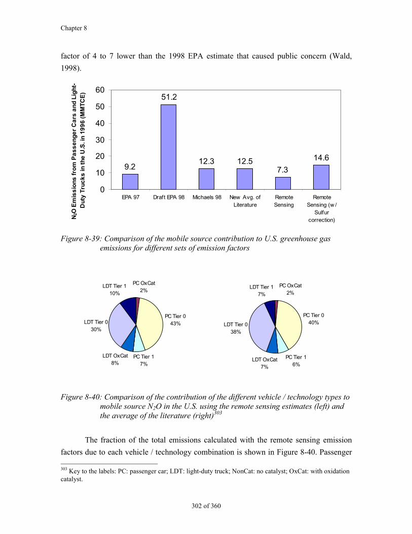
Chapter 8

302 of 360

factor of 4 to 7 lower than the 1998 EPA estimate that caused public concern (Wald,

1998).

9.212.3 12.5

7.3

14.6

51.2

0

10

20

30

40

50

60

EPA 97 Draft EPA 98 Michaels 98 New Avg. ofLiterature

RemoteSensing

RemoteSensing (w /

Sulfurcorrection)N

2O E

mis

sio

ns

fro

m P

as

se

ng

er

Ca

rs a

nd

Lig

ht-

Du

ty T

ruc

ks

in t

he

U.S

. in

19

96

(M

MT

CE

)

Figure 8-39: Comparison of the mobile source contribution to U.S. greenhouse gasemissions for different sets of emission factors

PC Tier 043%

PC Tier 17%

LDT Tier 030%

LDT Tier 110%

PC OxCat2%

LDT OxCat8%

PC Tier 040%

PC Tier 16%

LDT Tier 038%

LDT Tier 17%

LDT OxCat7%

PC OxCat2%

Figure 8-40: Comparison of the contribution of the different vehicle / technology types tomobile source N2O in the U.S. using the remote sensing estimates (left) andthe average of the literature (right)303

The fraction of the total emissions calculated with the remote sensing emission

factors due to each vehicle / technology combination is shown in Figure 8-40. Passenger 303 Key to the labels: PC: passenger car; LDT: light-duty truck; NonCat: no catalyst; OxCat: with oxidationcatalyst.

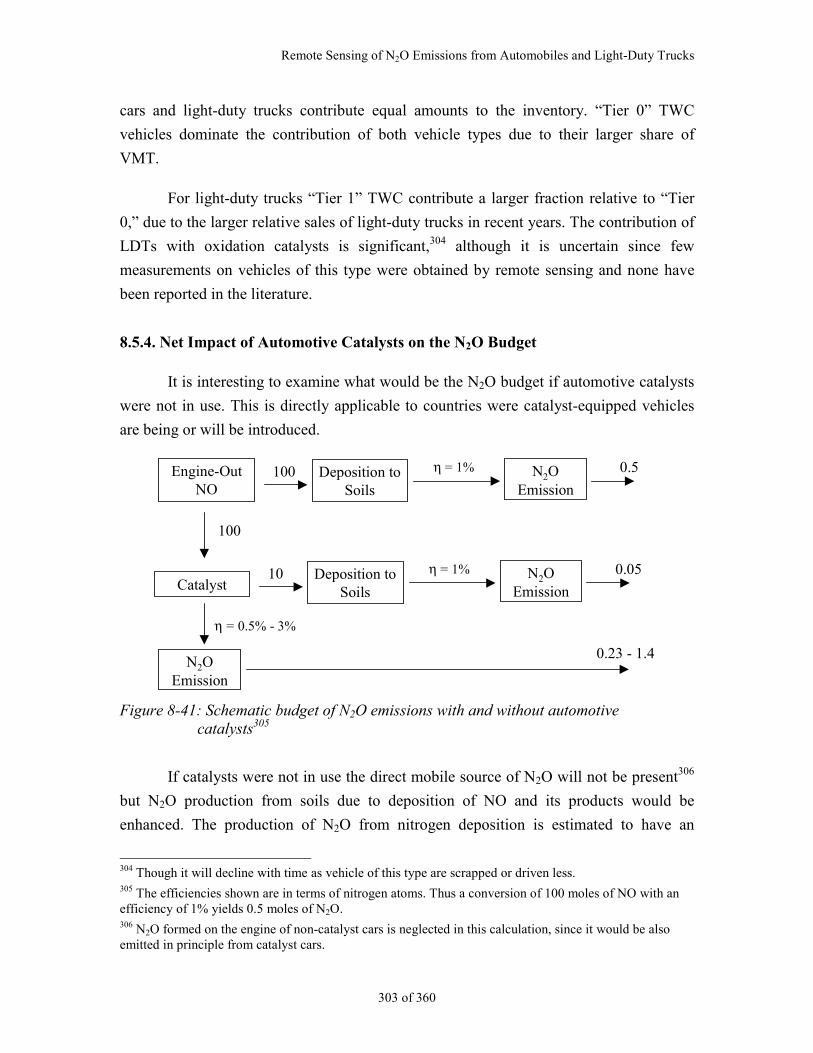
Remote Sensing of N2O Emissions from Automobiles and Light-Duty Trucks

303 of 360

cars and light-duty trucks contribute equal amounts to the inventory. “Tier 0” TWC

vehicles dominate the contribution of both vehicle types due to their larger share of

VMT.

For light-duty trucks “Tier 1” TWC contribute a larger fraction relative to “Tier

0,” due to the larger relative sales of light-duty trucks in recent years. The contribution of

LDTs with oxidation catalysts is significant,304 although it is uncertain since few

measurements on vehicles of this type were obtained by remote sensing and none have

been reported in the literature.

8.5.4. Net Impact of Automotive Catalysts on the N2O Budget

It is interesting to examine what would be the N2O budget if automotive catalysts

were not in use. This is directly applicable to countries were catalyst-equipped vehicles

are being or will be introduced.

Engine-OutNO

Deposition toSoils

N2OEmission

100 η = 1% 0.5

CatalystDeposition to

SoilsN2O

Emission10 η = 1% 0.05

η = 0.5% - 3%

100

N2OEmission

0.23 - 1.4

Figure 8-41: Schematic budget of N2O emissions with and without automotivecatalysts305

If catalysts were not in use the direct mobile source of N2O will not be present306

but N2O production from soils due to deposition of NO and its products would be

enhanced. The production of N2O from nitrogen deposition is estimated to have an

304 Though it will decline with time as vehicle of this type are scrapped or driven less.305 The efficiencies shown are in terms of nitrogen atoms. Thus a conversion of 100 moles of NO with anefficiency of 1% yields 0.5 moles of N2O.306 N2O formed on the engine of non-catalyst cars is neglected in this calculation, since it would be alsoemitted in principle from catalyst cars.

Chapter 8

304 of 360

efficiency of about 1% (Bouwman et al., 1995), though this estimate is highly uncertain.

The use of automotive catalysts increases direct N2O emissions. From the results in

section 8.4.1 we can estimate an N2O selectivity in the catalyst of 0.5%-3%. Comparing

both situations in Figure 8-41 we find that a significant part of the increased N2O

formation in the catalyst may be offset by decreased N2O formation in soils, thus

lowering the overall impact of introducing three-way catalysts.

Remote Sensing of N2O Emissions from Automobiles and Light-Duty Trucks

305 of 360

8.6. Discussion

8.6.1. Conclusions of the Experimental Results and the Analysis of the Literature

The main conclusions of this study with respect to N2O emissions from catalyst-

equipped vehicles are:

The N2O emissions of vehicles on several driving cycles are correlated, which

indicates that the tendency to emit more or less N2O is a characteristic of each

vehicle. Based on the limited data available, remote sensing is a useful technique for

measuring the N2O emission levels of catalyst-equipped vehicles.

The TILDAS technique is able to remotely measure N2O emissions with an average

fleet detection limit of ~8 ppm of the exhaust.

Measuring N2O emissions in inspection and maintenance programs using IM240

could provide very detailed information about N2O emissions which can be used to

better estimate the strength of this source and to investigate the causes of high N2O

emissions.

Both the remote sensing and the literature distributions of N2O emissions from

catalyst vehicles are highly skewed. This is the main reason for the conflicting N2O

emission factors for mobile sources.

High N2O emitters are not the necessarily the same as NO, CO or HC emitters. All

model years have a significant high emitter fraction.

N2O Emission rates were found to be more constant with vehicle age than those for

NO, CO or HC. The contribution of each model year from 1983 to 1996 to total

emissions is similar at about 7%.

Light-duty trucks were found to have higher emissions than passenger cars. About 1/2

of this difference can be explained by the fuel economy difference and the other 1/2 is

due to increased N2O generation for light-duty trucks per unit mass of fuel.

N2O emissions show some correlation with NO emissions. The results of this study

are consistent with N2O formation being proportional to the amount of NO reduced in

Chapter 8

306 of 360

the catalyst. The constant of proportionality is larger for higher NO emitters, which

can be explained by catalyst aging.

N2O emissions increase with vehicle specific power, but not as much as NO

emissions.

N2O emissions from remote sensing are about a factor of 7 lower than the 1996 IPCC

estimates and a factor of 1.6 lower than the average of the literature values and the

newest EPA estimates. This difference is tentatively attributed to the lower-sulfur

content of California’s gasoline, although insufficient data exist to confirm this point.

The contribution of gasoline on-road motor vehicles to U.S. greenhouse gas

emissions is estimated at 0.46%-0.92% based on the literature and on this study. This

is a factor of 4 to 7 lower than the 1998 Draft EPA estimate and brackets the newest

EPA estimate.

Sulfur reduction in gasoline may be an effective way to reduce N2O emissions from

catalyst-equipped vehicles. Further research on this topic is needed.

8.6.2. N2O High Emitters

High N2O emitters are different from CO, HC, or NOx high emitters. Remote

sensing could be used to detect vehicles with excess N2O emissions. Little is known

about the vehicle characteristics that lead to high N2O emissions, besides catalyst aging.

Catalyst replacement would probably reduce N2O emissions from high emitters but at a

significant cost. Further study of high emitter characteristics and repair strategies is

needed before the feasibility of this approach to reduce N2O emissions can be evaluated.

Repair strategies that would result in simultaneous reductions of other regulated

or unregulated pollutants would be easiest to implement in the U.S., because they will

provide an incentive to the states to implement them. Actions that are geared exclusively

towards the N2O emissions will be more difficult to implement.

The determination of vehicle or catalyst characteristics that result on high N2O

emissions may allow the avoidance of such characteristics on future vehicles. Remote

sensing or IM240 data with very large vehicle samples307 could provide the real-world

data needed for such a study. 307 It is estimated that at least 20,000 vehicles would be necessary to start to see stable statistics.

Remote Sensing of N2O Emissions from Automobiles and Light-Duty Trucks

307 of 360

8.6.3. Lowering Sulfur Gasoline for Reducing N2O Emissions

Based on the very limited data acquired recently by EPA (Michaels, 1998) and the

comparison between remote sensing and literature results, decreasing fuel sulfur may be a

viable strategy to reduce N2O emissions.

Fuel sulfur reduction programs are already in place in the U.S., Europe, and Japan

as a way to increase catalyst efficiency for CO, HC, and especially NOx (U.S. EPA,

1998d; Walsh, 1998b). California and Japan have already adopted a 30 ppm sulfur limit

and Europe has adopted a reduction in steps, reaching 150 ppm in 2000 and 50 ppm in

2005 (Walsh, 1998b). Canada recently announced a phased program to reach 30 ppm in

2005 (Environment Canada, 1998). Further reductions are being debated, with a coalition

of automobile manufacturers supporting a worldwide target of 30 ppm sulfur and the oil

industry resisting such efforts (ES&T, 1998). EPA recently concluded that a program

limiting sulfur content of gasoline is necessary for the reduction of the regulated

pollutants and has yet to decide on the form and limits of such a program (U.S. EPA,

1998d).

Gasoline sulfur reduction may be an important method way to reduce N2O mobile

source emissions. If a low-sulfur gasoline program was implemented nationwide, a

reduction of about ½ of the N2O emissions from catalyst-equipped vehicles could be

achieved, based the very limited data currently available.308 This could mean a reduction

of the order of 0.5 % of the U.S. greenhouse gas emissions.309 This is a very sizeable

reduction that will significantly help for the implementation of the Kyoto protocol.

The total estimated cost would be about US$5.4 billion,310 or $868 per ton of

carbon equivalent (TCE) if all the cost is attributed to the N2O reduction. This is

relatively expensive in comparison with the $100 to $200 per TCE of the most expensive

solutions estimated to be needed for compliance with the Kyoto protocol in the U.S.

(Ellerman and Decaux, 1998). Consequently, a sulfur reduction program may be too

expensive if the only objective was to reduce N2O emissions. N2O reduction, however, is

308 The reduction will come immediately if the sensitivity of N2O to fuel sulfur of “Tier 0” and oxidationcatalyst vehicles is the same than for the “Tier 1” and LEVs tested by Michaels (Michaels, 1998). If N2Ofrom “Tier 0” vehicles is in fact insensitive to sulfur reductions the N2O reduction will come as “Tier 0”vehicles are replaced by “Tier 1” and low-emission vehicles by fleet turnover.309 In terms of global warming potential (MMTCE).310 Assuming a cost of 5 cents per gallon of gasoline for sulfur removal (Cackette, 1998; U.S. EPA, 1998d)and a gasoline consumption by light-duty vehicles and light-duty trucks of 308.7⋅106 kg (Davis, 1997).

Chapter 8

308 of 360

an additional benefit that should be considered when analyzing gasoline sulfur reduction

programs for CO, HC, and NOx reduction purposes. Currently EPA is considering

whether to implement national, year-round sulfur limits, or local, seasonal limits (U.S.

EPA, 1998d). A permanent, national program will provide the most N2O benefit.

309 of 360

Chapter 9. Directions for Future Research

The findings reported in this thesis suggested many new interesting research

questions about vehicle emissions. This chapter summarizes some of the key future

research directions and some possible approaches for addressing them based on what was

learnt during this project.

9.1. Further Analysis of the Possibilities of Vehicle SpecificPower

The analyses presented in Chapter 3 demonstrate the usefulness of the new

definition of vehicle specific power for remote sensing and emission studies. Having a

single, readily measurable parameter that captures most of the dependence of vehicle

emissions on driving conditions opens up several important applications.

A New Structure for Emissions Models

Current inventory emission models such as MOBILE and EMFAC are based on

emission factors expressed in grams of pollutant per mile (gpm) traveled and estimates of

the vehicle-miles traveled. Speed correction factors are used to account for the effect of

driving conditions on emissions.

In this thesis it has been shown that the dependence of fuel consumption and

emissions in driving conditions is better captured by specific power (SP), and that

second-by-second emissions of light-duty vehicles are one to two orders of magnitude

more constant when expressed in grams of pollutant per gallon of fuel (gpg). These are

compelling reasons to base emissions models on SP and gpg.

Evaluation of Inspection and Maintenance Programs

A possible application of remote sensing is the evaluation of I/M programs

(Zhang et al., 1996b; Sjödin et al., 1997a; Stedman et al., 1998; U.S. EPA, 1998e). EPA

recently stated that it would approve this use “if RSD-measured fleet average emissions

can be correlated back to the IM240” (U.S. EPA, 1998e). Establishing the dependence of

Chapter 9

310 of 360

emissions on SP and weighing them by the SP distribution in the IM240 test could be

used for this purpose (see section 3.3.6 for a detailed description of this approach).

Reevaluation of High Emitter Detection in Remote Sensing

This study showed that SP can be used to screen out most of the occurrence of

commanded enrichment and enleanment operation, eliminating those sources of false

high emitter detection. This reopens the possibility of using remote sensing for this

important application, which should be evaluated taking into account economic

considerations.

Acquisition and Analysis of Second-by-Second Data from High Emitters

This thesis has shown that powerful insights can be gained from the analysis of

second-by-second operational and emissions data of vehicles operated in chassis

dynamometers. A data set of this kind with as many types of high emitters as possible

would allow the study of numerous questions, including the dependence of their

emissions on SP for these vehicles and the evaluation of the probability of detection with

remote sensing.

Directions for Future Research

311 of 360

9.2. Improved Quantification of Emissions from MobileSources

Large uncertainties remain in the estimates of the mobile source emissions

inventory. A number of research programs that could reduce these uncertainties are:

Detailed Study of the Emissions of Heavy-Duty Diesel Trucks

The successful remote sensing of heavy-duty diesel truck (HDDT) NOx opens the

possibility of exploring many interesting questions of the kind posed for automobile

emissions in Chapter 6 and Chapter 8. In particular, the variation of HDDTs emissions

vs. power can be studied. The concept of specific power, defined in Chapter 3, is also

applicable to HDDTs. However, due to the very large variations in vehicle weight for

these vehicles, HDDT remote sensing studies should also obtain this information.311

Long-Term Monitoring of Heavy-Duty Truck Emissions by Remote Sensing

By remotely sensing the emissions of heavy-duty trucks for a period of several

years, the rates of deterioration as well as the effects of emission reduction programs such

as diesel fuel reformulation, low-NOx diesel engines, or inspection and maintenance

programs can be determined. This information could then be used for the design of more

effective emission control strategies.

Measurement of heavy-duty truck emissions by low-pressure sampling

Low-pressure sampling could be an alternative to remote sensing for the

measurement of emissions from heavy-duty diesel trucks. A probe could be located at the

bottom of a highway bridge and a sample continuously drawn into a low pressure

multipass cell of a TILDAS instrument. This approach would yield sensitivities about

1,000 times larger than the remote sensing approach (Nelson et al., 1996) and would

permit the quantification of many more species besides NO and NO2.

Measurement of Emissions from Off-Road Mobile Sources

“Off-road mobile sources” refers to ships, trains, airplanes, and farm and

construction equipment. As on-road mobile source emissions have become increasingly

controlled, the estimates of the share of the less controlled off-road mobile sources in

311 From weight stations or weight-in-motion systems.

Chapter 9

312 of 360

total emissions has been increasing. These sources are not as well quantified as those of

on-road mobile sources.

An NDIR-UV remote sensor has been recently applied to the measurement of

aircraft emissions (Popp et al., 1998b), but the measurement was constrained by the

pathlength limitations of the technique. This same remote sensor will be used to measure

train locomotive emissions in the near future (Popp, 1998).

The TILDAS technology is ideally suited for remote sensing measurements of

off-road mobile sources such as airplanes and ships due to its larger range and excellent

sensitivity. Some potential applications would be the measurement of the emissions from

airplanes across airport runways and of ships in large harbors.

Directions for Future Research

313 of 360

9.3. N2O Emissions from Mobile Sources

Better Quantification of N2O Emissions from Mobile Sources

N2O emissions from catalyst-equipped vehicles were estimated to account for

0.5% to 0.9% of U.S. greenhouse emissions based on the results of this study. However,

very large uncertainties remain, and additional research its needed in this topic. A number

of approaches could provide better information about the magnitude of N2O emissions:

Cold start emissions could be quantified with remote sensing by measuring

the emissions from cars which have been parked for significant time at several

distances from the parking lot. Two possibilities would be an airport and a

stadium. This experiment would provide a profile of average N2O vs. distance

(or time) in cold start that may allow a more precise estimation of cold start

emission factors.

Remote sensing and/or IM240 can provide good estimates of real world

emission factors. Both systems would provide large, unbiased samples. They

would also allow the study of which vehicle/catalyst characteristics are

correlated with high N2O emission.

Repeating the same test (e.g. remote sensing or IM240 tests) under the same

conditions each year or few years would provide a robust estimate of the

evolution of these emissions. A program like this one for CO, HC, and NO is

now in its second year with remote sensing.

Ambient N2O/CO2 in a urban area where other N2O and CO2 sources are well-

characterized can be used to obtain a driving-mode integrated N2O/CO2

emission factor. Such an approach has been used for estimating CH4

emissions (Shorter et al., 1996).

N2O emissions are highest during starts. Some emissions models such as

EMFAC account for cold and hot start excess emissions separately.

Integrating that approach with cold start emission estimates for the U.S. would

probably improve the inventory estimate.

Chapter 9

314 of 360

The current N2O estimates are based on grams-per-mile and vehicles-mile

traveled. Estimates based on grams-per-gallon and fuel should be used as an

alternative check on the inventory.

Reduction of N2O Emissions Through the Reduction of Gasoline Sulfur

The above estimate indicates that N2O emissions from catalyst-equipped vehicles

are not negligible with regard to the limitations that may be needed to comply with the

1997 Kyoto protocol, and that the possibilities for its reduction should be investigated.

It was recently observed that lower gasoline sulfur content results in reduced N2O

emissions (Michaels, 1998). Sulfur levels are being reduced worldwide (Walsh, 1998b).

EPA has yet not decided whether to implement sulfur limits in some areas and

seasonally, or nationally and permanently (U.S. EPA, 1998d). This issue is highly

controversial, with the oil companies advocating the less stringent programs and the

automobile manufacturers the most stringent (ES&T, 1998).

This effect needs to be better quantified better in order to evaluate the potential

reductions that could be achieved by lower gasoline sulfur. Current data are limited to

two Tier 1 vehicles and three low emission vehicles (Michaels, 1998). No data on Tier 0

vehicles, which comprise most of the fleet, exist. Dynamometer cycle testing of a larger

sample (including Tier 0 vehicles) with both high and low sulfur gasoline could provide

the data needed. Alternatively carrying out remote sensing measurements (or

measurements during IM240 testing) before and after the gasoline sulfur level is changed

on a given area would provide robust real-world estimates of the effect of sulfur on N2O.

Studies of this kind have provided insights on the effect of reformulated gasoline on CO,

HC, and NOx emissions (Bishop and Stedman, 1990).

Investigation of the Causes of High N2O Emissions

This study has shown that the N2O emissions distribution is highly skewed, and

that the concept of “super-emitter” is applicable to N2O. For example the ratio of the

maximum N2O emission from a car to the average level of all cars was 47, compared to

only 12 for NO.

A N2O remote sensing campaign with a large number of vehicles or the

integration of N2O emission measurements in IM240 programs would allow the study of

whether specific manufacturers or vehicle models tend to have much higher N2O

Directions for Future Research

315 of 360

emissions than the rest. A similar analysis for regulated pollutants using remote sensing

and IM240 data has been able to pinpoint specific models with emission control system

problems (Wenzel et al., 1996; Wenzel et al., 1997).

It would also be of great interest to identify and borrow the few highest emitters

and study what vehicle characteristics may be causing such high N2O emission. This

information may then be used for achieving lower N2O emissions from new vehicles, and

also for repairing high N2O emitters, if repairs were determined to be a cost-effective

alternative or if they could be done simultaneously with repairs for other pollutants.

Chapter 9

316 of 360

9.4. Quantification of Ammonia Emissions from Three-WayCatalyst Equipped Vehicles

Ammonia (NH3) is very important for fine particulate matter and acid deposition.

While NH3 is present in the exhaust of internal combustion engines, both gasoline and

diesel, three-way catalysts increase NH3 emissions from gasoline vehicles. Conflicting

emission factors are reported in the literature for three-way catalyst equipped vehicles.

Emission rates up to 268 mg/mi have been reported when cars were forced to run with

rich air-fuel mixtures (Cadle and Mulawa, 1980). Moeckli et al. (Moeckli et al., 1996)

report a range from 5 to 24 mg/mi based on a tunnel study in Switzerland. Two recent

studies have reported significant amounts of NH3 in the vehicle exhaust. Baum (Baum,

1997) measured concentrations of up to 628 ppm in the exhaust of TWC-equipped cars,

and reported that NH3 was larger when the engine was running under lean conditions, in

contradiction to Cadle and Mulawa’s findings. Fraser and Cass (Fraser and Cass, 1998)

reported an average emission rate of 116 mg/mi for three-way catalyst cars, based on a

tunnel study in the Los Angeles area.

Some catalyst studies suggest that the chemistries of N2O and NH3 in the catalyst

are tightly linked (Cant et al., 1998; Odaka et al., 1998), and that NH3 is formed in the

catalyst from NO at relatively low temperatures (Cant et al., 1998), lower than those of

maximum N2O production. If this is indeed the main process producing NH3 from TWC-

equipped cars, NH3 emissions from light-duty vehicles will be largest for vehicles under

cold-start conditions.

Quantification and Understanding of NH3 Emissions from Motor Vehicles

Many questions remain about the magnitude and the mechanism of formation of

NH3 emissions from TWC-equipped vehicles: What is the NH3 emission factor for each

type of vehicles? What is the nature of the NH3 emissions distributions? Are there NH3

high emitters? What are the NH3 emissions in cold start vs. hot stabilized conditions?

What is the correlation of NH3 emissions with vehicle characteristics (passenger cars vs.

light-duty trucks, emission control technology, model year, manufacturer, etc.)? With

vehicle operating conditions (speed, acceleration, specific power)? With other emissions

(CO, HC, NO, N2O)? This information would help understand the importance of the

problem, the processes by which NH3 is emitted from vehicles, and give clues as to ways

or reducing NH3 emissions from current and future vehicles.

Directions for Future Research

317 of 360

The same approaches outlined in the previous section for N2O can also be used

for NH3. Dynamometer testing, especially with collection of second-by-second data,

and/or TILDAS remote sensing312 could provide answers to some of these questions by

quantifying and characterizing NH3 emissions in the same way described in Chapters 6

and 8 of this thesis for NO and N2O, respectively.

Synergy with Research of N2O Emissions from TWC vehicles

Both NH3 and N2O are mostly incomplete byproducts of NO reduction in three-

way-catalysts. Both species should be measured simultaneously (by remote sensing or

during dynamometer testing) in order to shed light on the catalyst processes which may

result in elevated emissions.

312 We estimate that the TILDAS technique can perform NH3 remote sensing with good sensitivity.Ammonia has many individual strong infrared absorption features in the 875-1125 cm-1 region, with littleinterference from background air species or other species in car exhaust. A preliminary test performed atAerodyne Research in May 1998 indicated that the measurement is possible with the existing instrumentand that the sensitivity could be of the same order of that achieved for NO, depending on the laser diodeused.

Chapter 9

318 of 360

9.5. Further Development of the TILDAS Remote Sensor

Design of an Commercial TILDAS-only Remote Sensor

The TILDAS instrument used in this thesis is a one-of-a-kind laboratory type

instrument. It has shown impressive remote sensing capabilities and has produced results

suggesting that such measuring capability has great value. Simplifying the operation and

reducing the cost of the instrument are necessary tasks. Such a system would need to be

equipped with at least four diode lasers, to be able to measure CO, an HC surrogate, NO,

and CO2 simultaneously.

Comparison of TILDAS to other remote sensing technologies

The performance of the TILDAS remote sensor should be compared to that of the

other existing remote sensing technologies. Puffs from gas cylinders mounted on moving

cars, and remote sensing of emissions from low-emitting and high emitting vehicles

should be used for this purpose.

Design of a TILDAS Addendum to NDIR/UV Instruments

Another possibility is to design a TILDAS module that can be incorporated into

existing NDIR/UV instruments to provide measurements that those instruments cannot

acquire, such as N2O, NH3, C2H2, C2H4, CH4 or CH2O. Such a design would reduce the

cost and the operational requirements of the TILDAS instrument.

319 of 360

Chapter 10. Conclusions

Air pollutant emissions from motor vehicles are a large contributor to many

important environmental problems, including local and regional air quality and the

increased greenhouse effect. The first regulations controlling emissions from motor

vehicles were established 33 years ago (1965) in California and since then have spread to

most countries and become increasingly stringent. The emission reductions achieved

through the successive control strategies, however, have been smaller than anticipated.

That fact, combined with the continuous increase in the use of motor vehicles, means that

on-road motor vehicles are, and will continue to be in the foreseeable future, a major

source of air pollutants around the world and that further control is needed.

Despite their importance, real-world motor vehicle emissions are still

unsatisfactorily quantified and understood, owing to the many factors that influence the

emissions of each individual vehicle, and to the difficulty of characterizing hundreds of

millions of them. This thesis presents several significant contributions that address these

basic problems in the following ways:

First, a new, directly measurable parameter (specific power) was defined and shown

to capture most of the dependence of light-duty vehicle emissions on driving

conditions. The use of this parameter could simplify emission studies and establish a

common language between the different emission research and modeling approaches.

Second, a new, TILDAS-based remote sensor was developed and tested which can

provide high quality real-world emission measurements on large vehicle samples,

including the emissions of the cleanest vehicles. Very high precision and long

pathlenth were demonstrated.

Third, this new remote sensor was used to answer some of the outstanding questions

about mobile source emissions by conducting 2 experimental field campaigns where

the emissions of about 1,500 random cars and light-duty trucks, a instrumented

heavy-duty diesel truck, and 73 random heavy-duty diesel trucks were measured.

These experiments provided the first high precision remote sensing data of NOx

emissions from passenger cars, light-duty trucks, and heavy-duty diesel trucks, plus

Chapter 10

320 of 360

the first remote sensing ever of N2O and NO2 emissions. An in-depth analysis of

these data was carried out.

The detailed conclusions of this work are summarized below:

A new parameter for emission studies

Vehicle specific power (SP) is defined as the mechanical power used for the

vehicle’s motion. This parameter has a number of important advantages for remote

sensing and emission studies for three reasons:

SP is a better predictor of emissions that any other roadside measurable

parameter. In particular SP is a very good predictor of commanded enrichment

situations.

SP can be calculated with good approximation from measurements of vehicle

speed and acceleration.

Dynamometer driving cycles used for emission certification of new vehicles

directly specify the value of SP (and not the total power or fraction of

available power) at each second in the cycle. Evidence is presented that

automobile designers make use of this fact.

These properties make SP an very useful parameter for emission studies. The

applications of this parameter include:

Specific power can be used to make meaningful comparisons between the

results of different dynamometer driving cycles, experimental emission

studies, remote sensing studies, and emission models. This would be a great

improvement over the status quo in which the differences in power demand

obscure the comparisons.

Specific Power is highly valuable for the interpretation of remote sensing

measurements. It allows more precise identification of high emitters by

screening out remote sensing measurements under conditions that lead to

transient high emissions in properly functioning vehicles, since these

emissions may not be repairable through an inspection and maintenance

program. Low-emitter identification can be improved as well.

Conclusions

321 of 360

Emissions models can benefit from using Specific Power as the main

parameter to represent load since this parameter has a strong relationship with

emissions and is directly measurable in the real world. Inventory models such

as MOBILE and EMFAC would be improved by using SP correction factors

to replace the speed correction factors that they now use to account for

differences in driving conditions.

An in-depth analysis of remote sensing measurements

Remote sensing of on-road vehicle emissions was pioneered by Don Stedman and

Gary Bishop of the University of Denver in 1987. Together with several other groups and

companies, they have made remote sensing measurements on millions of vehicles.

However, some basic aspects of the measurements have not been studied or documented

until now. Several important topics have been addressed here:

The signal levels observed in remote sensing measurements (“plume capture”)

are highly variable due to changes in the amount of exhaust gases emitted

with power, and especially due to differences in plume dispersion.

Experimentally plume capture decreases with vehicle speed and increases

with power demand at a constant speed.

Plume capture in the heavy-duty diesel truck measurements was about twice

as large than on the automobile measurements, which can be explained by 4

times more CO2 flow and twice as strong dispersion.

The noise in the remote sensing measurements depends both on plume capture

and on the level of the pollutant measured. High plume captures and low

pollutant concentrations yield the best precision while low plume captures and

high pollutant concentrations result in lower absolute precision. These effects

should be taken into account when using remote sensing measurements for the

detection of low and/or high emitters.

The location of interest for the speed and acceleration measurements taken in

conjunction with remote sensing measurements is where the exhaust which is

leaving the tailpipe was generated in the engine. This distance has been

estimated to vary between 0.1 and 25 meters for one vehicle. Smaller

distances correspond to low speed and high specific power, and large

distances to high speed and low specific power. The consequence is that a

Chapter 10

322 of 360

fixed location speed and acceleration measurement may not be sufficient for

the determination of the appropriate specific power. It is suggested that an

array of low-cost diodes is used to determine the speed and specific power

profile of each vehicle as it approaches the remote sensor.

Second-by-second driving cycle emissions for a modern car are one to two

orders of magnitude less variable when expressed in units of grams of

pollutant per unit of fuel consumed than in grams per unit distance traveled. It

is suggested that gpg emission factors should be used in emission inventories

and models for this reason.

The development and demonstration of a laser-based remote sensor

Current remote sensors are limited in sensitivity and range. The use of tunable

diode laser spectroscopy (known as TDL spectroscopy, TLDAS or TILDAS) in remote

sensing can help overcome those limitations.

In this study a TILDAS instrument has been modified for use as a remote sensor

of vehicle emissions. It operates two diode lasers in two different frequency regions. The

average sensitivity of the instrument is estimated at 5 ppm fo the exhaust for NO and 4

ppm for N2O under real-world conditions. This sensitivity has been demonstrated by

measuring the emissions of an Ultra Low Emission Vehicle (ULEV). The TILDAS

measurements compared very well with the simultaneous measurements of the on-board

system of an instrumented heavy duty truck.

The main advantages of the TILDAS technique for its application to remote

sensing of vehicle emissions are:

The high sensitivity of the technique, which allows the measurement of the emissions

from even the cleanest vehicles.

The unique ability of this technique to remotely sense minor species of interest in

automotive exhaust such as NO2, NH3, N2O, formaldehyde, and other small

hydrocarbons.

The absence of interferences from other gases or particulates in the vehicle exhaust or

in ambient air, or from infrared emission from the vehicle or the exhaust, due to the

its very high spectral resolution and fast time response.

Conclusions

323 of 360

The higher information content of the technique with respect to NDIR or NDUV

make it more robust against anoumalous effects such as interferences from the

exhaust of previous vehicles, vibrations, etc.

The absolute nature of this technique, which makes repeated calibrations unnecessary.

Other techniques require frequent field calibration to resist inherent drifts.

The longer path length achievable with this technique with only minor degradation of

sensitivity, due to the coherent nature of laser radiation. Measurements of NO/CO2

ratios over a total pathlength of 88 meters (289 ft) have been demonstrated. This is

more than 7 times longer than those reported for NDIR-based instruments.

This fact eliminates the need for constricting the traffic, alleviates safety concerns,

and provides much more freedom in choosing remote sensing sites. The authors of the

Texas Remote Sensing Feasibility study (Walsh et al., 1997) conclude that finding

adequate sites was very difficult in some urban areas.

The Texas study also found that for repeated measurements in the same location, the

first reading was higher 60% of the time, which they attribute to changes on driving

behavior after noticing the presence of the remote sensor. The longer paths achievable

with TILDAS would allow the instrument to be hidden from motorists, eliminating

this potential source of measurement bias.

Exhaust gases may have elevated temperatures as they leave the tailpipe, and

quickly cool down as they mix with ambient air. These elevated temperatures may be

detectable by the TILDAS instrument, depending on the absorption lines being used.

Little effect was observed in the automobile measurements, while significant effects

appeared in the heavy-duty diesel truck NO/CO2 measurements. A numerical

optimization scheme was successfully developed to allow the estimation of the gas

temperatures from the remote sensing spectra.

Chapter 10

324 of 360

The first high precision remote sensing measurements of NO emissions from a large real-

world fleet

Remote sensing of on-road NO emissions has lagged with respect to CO and HC

emissions due to instrumentation problems. This study reported the first remote sensing

measurements of NO emissions with a high precision instrument from a large fleet of cars

and light-duty trucks. This study yielded a number of significant new findings with

respect to the NO emissions of on-road vehicles and the utility of remote sensing

emissions measurements:

The TILDAS instrument consistently and accurately measured the NO emissions of

on-road vehicles. The NO emissions of low emitters were measured with an average

precision of about 5 ppm.

The measured vehicle fleet NO emissions closely fit a gamma distribution with the 10

percent of the fleet having the highest emissions contributing about 50 percent of the

total fleet emissions.

The NO emission factor in this study is about 80% of those measured in 3 recent

tunnel studies in California. The reason for this lower emission is not clear.

Newer vehicles have lower average NO emissions than older ones but high NO

emitters are found in every vehicle age cohort.

The light-duty trucks in this study are higher NO emitters than passenger cars. About

½ of the difference is due to their lower fuel economy while the other ½ reflects

higher NO exhaust concentrations, possibly due to more lenient emission standards.

The EMFAC emission model accurately predicts the NO emissions of recent model

years in our study and overestimates those of older vehicles.

Analysis of the NO data with respect to the other simultaneously recorded data for the

subject vehicles shows that on a vehicle-by-vehicle basis NO emissions correlate only

weakly with vehicle specific power, speed, acceleration, CO emissions or HC

emissions. High NO emitting vehicles cannot be identified by remote sensing of CO

or HC emissions and vice versa. When these same data are aggregated into rank

ordered population deciles, positive correlations between decile averaged NO

Conclusions

325 of 360

emissions and the decile averaged values of vehicle specific power, CO, and HC for

most of the vehicles appear.

When we compared the remotely sensed NO emissions measurements for 117

vehicles measured more than once, most of them were consistently low emitters.

About half of the high NO emitters were found to be consistently high while the other

half had significant variability.

The 10% highest emitters for each of CO, HC, and NO in this study constitute a

group of 23% of the vehicles responsible for more than of 60% of the emissions of

each pollutant.

Vehicles manufactured by Honda showed statistically significant lower NO emissions

than the rest of the fleet for model years 93-96. This was mostly due to the lack of

high emitters in the Honda fleet. Significant differences in high emitter incidence

among makes also appear in a large database of inspection and maintenance data

from Arizona. An important implication is that emissions could be significantly

reduced by providing the manufacturers with incentives for the design of emission

control systems with lower failure rates.

Remote sensing of NO and NO2 emissions from heavy-duty diesel trucks

Heavy-duty trucks are a large contributor to the on-road NOx inventory. In this

study the TILDAS instrument was used to remotely sense the NO and NO2 emissions of

heavy-duty diesel trucks (HDDTs). These experiments yielded a number of significant

new findings with respect to remote sensing of heavy-duty diesel truck (HDDT)

emissions and their NOx emission factors:

The NOx emissions of HDDTs can be measured by TILDAS remote sensing under

real world conditions with very good accuracy and precision. Very good agreement

between the measurements of the EPA instrumented truck and the TILDAS

instrument was achieved.

Based on the results of this study the magnitude of HDDT NOx emissions is

underestimated by a factor of 2.2 in the U.S. The share of HDDTs on mobile source

NOx is larger than that of automobiles and light-duty trucks, with an estimated share

of 58% of the on-road NOx inventory. These results imply that as much effort needs

to be done to reduce HDDT NOx emissions as has been done for light-duty vehicle

Chapter 10

326 of 360

NOx, if further meaningful improvements in mobile source NOx-related air quality

problems are to be achieved.

The HDDT NOx emission factors are remarkably constant across several tunnel and

remote sensing studies. Thus the inventory contribution of HDDT NOx may be

reliably estimated from these emission factors.

The HDDT NOx emission distribution, unlike the distribution for light-duty vehicles,

is not highly skewed. The nature of the distributions of NOx emissions from light-

duty gasoline and heavy-duty diesel vehicles is shown to be directly related to the

nature of the engine and emission control system.

The concept of “super-emitter” is not applicable to HDDTs for NOx, since the

differences between the lowest and the highest emitters are just a factor of 6.5,

compared to a factor of 750 for automobiles. A consequence of this fact is that the

potential of significant reductions on emissions through targeting an inspection and

maintenance program on the high emitters (or savings by clean-screening low

emitters) is small for HDDTs. Conversely, approaches that deal with the whole fleet

such as emission standards and reformulated diesel fuel have the largest potential.

The first remote sensing measurements of N2O emissions from passenger cars and light-

duty trucks

The catalytic converter used to reduce the emissions of CO, HC, and NOx in cars

and light-duty trucks increases the emissions of nitrous oxide (N2O), which is an

important greenhouse gas and also causes stratospheric ozone depletion. The total amount

of N2O emitted to the atmosphere due to this source is highly uncertain. This study

reports the first on-road remote sensing measurements of N2O and a thorough

compilation of the literature studies that measured N2O emissions from vehicles. A

number of significant new findings include:

The N2O emissions of different vehicles on several driving cycles are highly

correlated, which indicates that the tendency to emit more or less N2O is a

characteristic of each vehicle. Measuring N2O emissions in inspection and

maintenance programs using IM240 could provide very detailed information about

N2O emissions.

Conclusions

327 of 360

Based on the limited data available, remote sensing is appropriate for measuring N2O

emissions from catalyst-equipped vehicles. The TILDAS technique is able to

remotely sense the N2O emissions of low-emitters with a fleet average sensitivity of

about 8 ppm of the exhaust.

Both the remote sensing and the literature distributions of N2O emissions from

catalyst vehicles are highly skewed, and the concept of “high emitter” is applicable to

N2O emissions. The presence or absence of high emitters in the small vehicle samples

tested in most previous studies is the main reason for the conflicting N2O emission

factors for mobile sources.

High N2O emitters not the necessarily the same as NO, CO or HC emitters. All model

years have a significant high emitter fraction.

N2O Emission rates were found to be more constant with vehicle age than those for

NO, CO or HC. The contribution of each model year from 1983 to 1996 to total

emissions is similar at about 7%.

Light-duty trucks were found to have higher emissions than passenger cars. About ½

of this difference can be explained by the fuel economy difference and the other ½ is

due to increased N2O generation for light-duty trucks.

N2O emissions show some correlation with NO emissions. The results of this study

are consistent with N2O formation being proportional to the amount of NO reduced in

the catalyst. The constant of proportionality is larger for higher NO emitters, which

can be explained by catalyst aging.

N2O emissions increase with vehicle specific power, but not as much as NO

emissions.

N2O emissions from remote sensing are about a factor of 7 lower than the 1996 IPCC

estimates and a factor of 1.6 lower than the average of the literature values and the

newest EPA estimates. The former estimate is too high due to a poor use of the

literature sources. The difference with the later estimates is tentatively attributed to

the lower-sulfur content of California’s gasoline, though insufficient data exist to

confirm this point.

Chapter 10

328 of 360

When a correction for the sulfur content of gasoline is used, the corrected remote

sensing and literature average N2O emission factors are about a factor of 3-5 lower

than the IPCC 96 estimates and slightly higher than the latest EPA estimates.

The contribution of passenger cars and light-duty trucks to net 1996 U.S. greenhouse

gas emissions is estimated at 0.46 %-0.92% based on the literature and on this study.

This is a factor of 4 to 7 lower than the 1998 Draft EPA estimate and very similar to

the newest EPA estimate.

Sulfur reduction in gasoline may be an effective way to reduce N2O emissions from

catalyst-equipped vehicles.

329 of 360

Chapter 11. Appendix

Appendix A. Units Used for Emission Factors

Four units which are commonly used to express motor vehicle emission factors

are. This section presents their definition and the conversions between them.

1. the mixing ratio of a given species on the exhaust gases, expressed as percent or

parts-per-million (ppm). This is the same as the molar fraction or volume fraction of

that species. Two variations exists, the so called “wet basis” and “dry basis.”

On the “wet basis,” (used in this thesis) the mixing ratio is calculated as the

molar fraction of the given species with respect to all the molecules in the

exhaust, including water.

On the “dry basis,” the mixing ratio is calculated as the molar fraction of the

species with respect to the exhaust excluding all water. This is done for

historical reasons because most sampling gas analyzers (such as NDIR

analyzers for CO2 and CO, or chemiluminescent analyzers for NOx) need to

operate with a dry feed gas, to avoid internal condensation.

To convert between the two unit systems one only has to know the mixing ratio of

water in the exhaust. For stoichiometric combustion of gasoline this mixing ratio is

12.5%, and the conversion between dry and wet basis is:

ion]Concentrat Wet[143.1

O][H-1

ion]ConcentratPollutant [Wet ion]ConcentratPollutant Dry[

2

∗=

==

2. The species/CO2 ratio. This is advantageous for example when dealing with diesel

engines, which have variable amounts of excess air which cannot be determined by

remote sensing. It is also the primary variable determined from remote sensors by

ratioing the measured column densities of each species. In order to be comparable

with other emission indices, the CO2 used in this ratio should be based on complete

combustion of the fuel. The following equation is used to correct for any incomplete

combustion products:

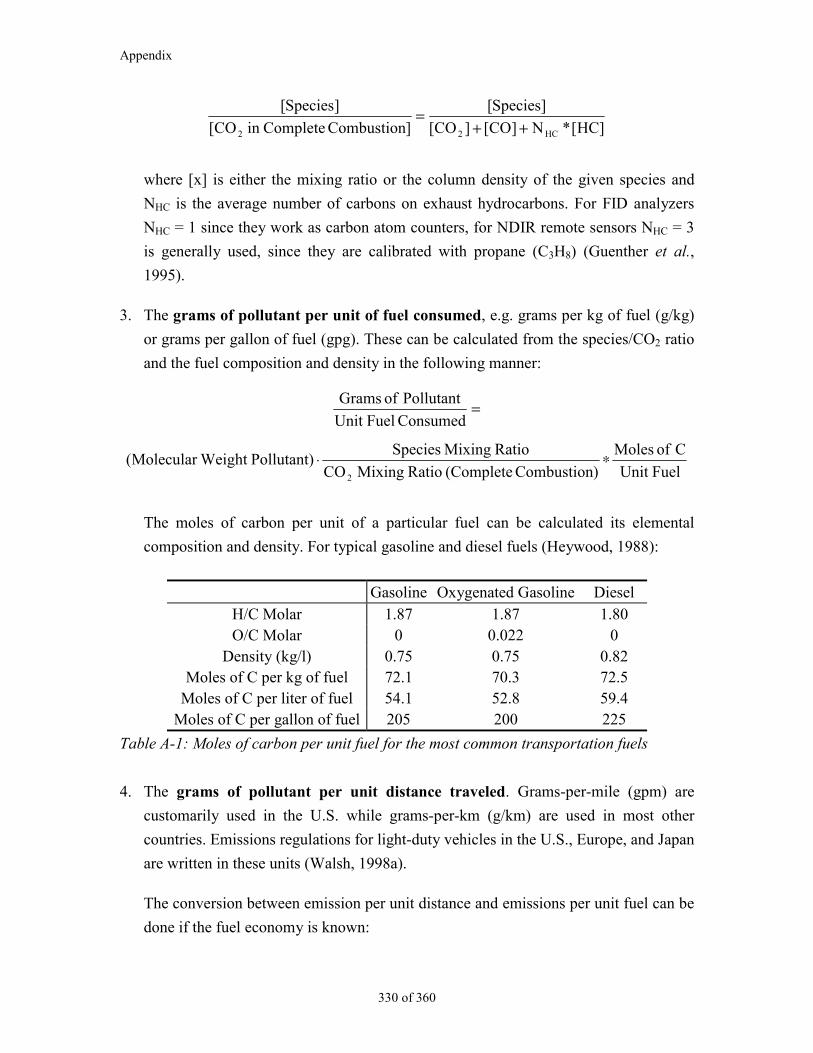
Appendix

330 of 360

]HC[*N]CO[]CO[

]Species[

]Combustion Completein CO[

]Species[

HC22 ++=

where [x] is either the mixing ratio or the column density of the given species and

NHC is the average number of carbons on exhaust hydrocarbons. For FID analyzers

NHC = 1 since they work as carbon atom counters, for NDIR remote sensors NHC = 3

is generally used, since they are calibrated with propane (C3H8) (Guenther et al.,

1995).

3. The grams of pollutant per unit of fuel consumed, e.g. grams per kg of fuel (g/kg)

or grams per gallon of fuel (gpg). These can be calculated from the species/CO2 ratio

and the fuel composition and density in the following manner:

FuelUnit

C of Moles

)Combustion (Complete Ratio Mixing CO

Ratio Mixing Species Pollutant) Weight Molecular(

Consumed FuelUnit

Pollutant of Grams

2

∗⋅

=

The moles of carbon per unit of a particular fuel can be calculated its elemental

composition and density. For typical gasoline and diesel fuels (Heywood, 1988):

Gasoline Oxygenated Gasoline Diesel

H/C Molar 1.87 1.87 1.80O/C Molar 0 0.022 0

Density (kg/l) 0.75 0.75 0.82Moles of C per kg of fuel 72.1 70.3 72.5

Moles of C per liter of fuel 54.1 52.8 59.4Moles of C per gallon of fuel 205 200 225

Table A-1: Moles of carbon per unit fuel for the most common transportation fuels

4. The grams of pollutant per unit distance traveled. Grams-per-mile (gpm) are

customarily used in the U.S. while grams-per-km (g/km) are used in most other

countries. Emissions regulations for light-duty vehicles in the U.S., Europe, and Japan

are written in these units (Walsh, 1998a).

The conversion between emission per unit distance and emissions per unit fuel can be

done if the fuel economy is known:

Appendix

331 of 360

DistanceFuel

Fuel Emission /Distance Emission / =

Or with the usual U.S. units:

mpg

gpggpm

consumed GallonsTraveled Miles

consumed Gallons/ pollutant of gramsTraveled Mile/ pollutant of grams

=⇒

=

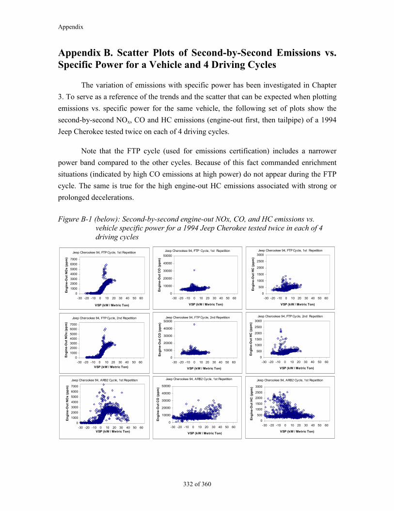
Appendix

332 of 360

Appendix B. Scatter Plots of Second-by-Second Emissions vs.Specific Power for a Vehicle and 4 Driving Cycles

The variation of emissions with specific power has been investigated in Chapter

3. To serve as a reference of the trends and the scatter that can be expected when plotting

emissions vs. specific power for the same vehicle, the following set of plots show the

second-by-second NOx, CO and HC emissions (engine-out first, then tailpipe) of a 1994

Jeep Cherokee tested twice on each of 4 driving cycles.

Note that the FTP cycle (used for emissions certification) includes a narrower

power band compared to the other cycles. Because of this fact commanded enrichment

situations (indicated by high CO emissions at high power) do not appear during the FTP

cycle. The same is true for the high engine-out HC emissions associated with strong or

prolonged decelerations.

Figure B-1 (below): Second-by-second engine-out NOx, CO, and HC emissions vs.vehicle specific power for a 1994 Jeep Cherokee tested twice in each of 4driving cycles

Jeep Cherookee 94, FTP Cycle, 1st Repetition

0

1000

2000

3000

4000

5000

6000

7000

-30 -20 -10 0 10 20 30 40 50 60

VSP (kW / Metric Ton)

En

gin

e-O

ut

NO

x (

pp

m)

Jeep Cherookee 94, FTP Cycle, 1st Repetition

0

10000

20000

30000

40000

50000

-30 -20 -10 0 10 20 30 40 50 60

VSP (kW / Metric Ton)

En

gin

e-O

ut

CO

(p

pm

)

Jeep Cherookee 94, FTP Cycle, 1st Repetition

0

500

1000

1500

2000

2500

3000

-30 -20 -10 0 10 20 30 40 50 60

VSP (kW / Metric Ton)

En

gin

e-O

ut

HC

(p

pm

)

Jeep Cherookee 94, FTP Cycle, 2nd Repetition

0

1000

2000

3000

4000

5000

6000

7000

-30 -20 -10 0 10 20 30 40 50 60

VSP (kW / Metric Ton)

En

gin

e-O

ut

NO

x (

pp

m)

Jeep Cherookee 94, FTP Cycle, 2nd Repetition

0

10000

20000

30000

40000

50000

-30 -20 -10 0 10 20 30 40 50 60

VSP (kW / Metric Ton)

En

gin

e-O

ut

CO

(p

pm

)

Jeep Cherookee 94, FTP Cycle, 2nd Repetition

0

500

1000

1500

2000

2500

3000

-30 -20 -10 0 10 20 30 40 50 60

VSP (kW / Metric Ton)

En

gin

e-O

ut

HC

(p

pm

)

Jeep Cherookee 94, ARB2 Cycle, 1st Repetition

0

1000

2000

3000

4000

5000

6000

7000

-30 -20 -10 0 10 20 30 40 50 60VSP (kW / Metric Ton)

En

gin

e-O

ut

NO

x (

pp

m)

Jeep Cherookee 94, ARB2 Cycle, 1st Repetition

0

10000

20000

30000

40000

50000

-30 -20 -10 0 10 20 30 40 50 60

VSP (kW / Metric Ton)

En

gin

e-O

ut

CO

(p

pm

)

Jeep Cherookee 94, ARB2 Cycle, 1st Repetition

0

500

1000

1500

2000

2500

3000

-30 -20 -10 0 10 20 30 40 50 60

VSP (kW / Metric Ton)

En

gin

e-O

ut

HC

(p

pm

)

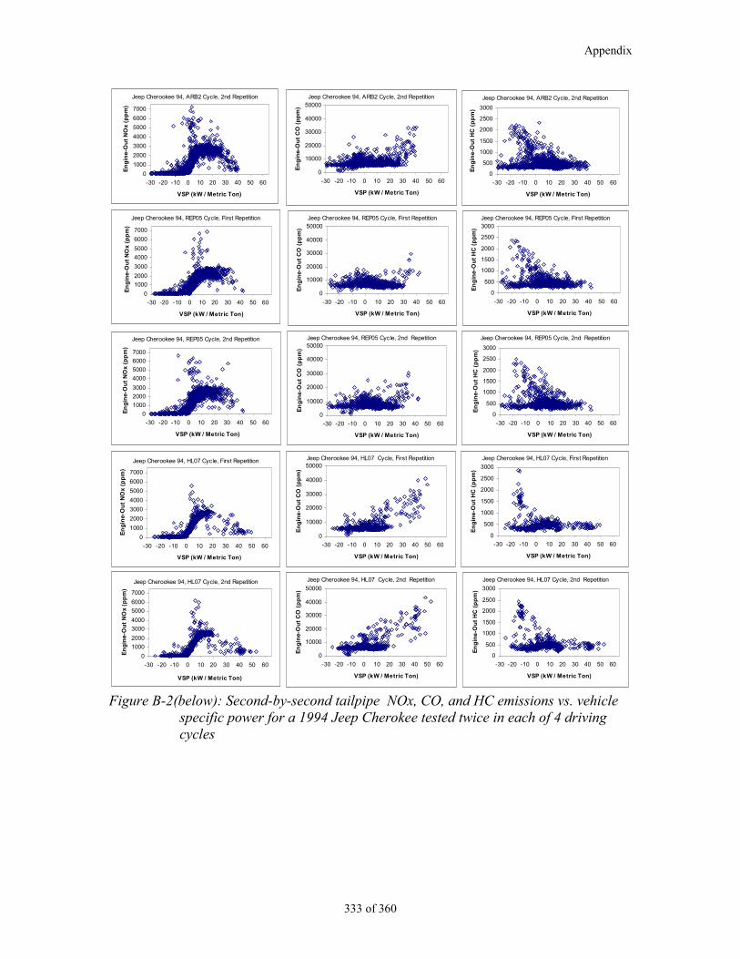
Appendix

333 of 360

Jeep Cherookee 94, ARB2 Cycle, 2nd Repetition

0

1000

2000

3000

4000

5000

6000

7000

-30 -20 -10 0 10 20 30 40 50 60

VSP (kW / Metric Ton)

En

gin

e-O

ut

NO

x (

pp

m)

Jeep Cherookee 94, ARB2 Cycle, 2nd Repetition

0

10000

20000

30000

40000

50000

-30 -20 -10 0 10 20 30 40 50 60

VSP (kW / Metric Ton)

En

gin

e-O

ut

CO

(p

pm

)

Jeep Cherookee 94, ARB2 Cycle, 2nd Repetition

0

500

1000

1500

2000

2500

3000

-30 -20 -10 0 10 20 30 40 50 60

VSP (kW / Metric Ton)

En

gin

e-O

ut

HC

(p

pm

)

Jeep Cherookee 94, REP05 Cycle, First Repetition

0

1000

2000

3000

4000

5000

6000

7000

-30 -20 -10 0 10 20 30 40 50 60

VSP (kW / Metric Ton)

En

gin

e-O

ut

NO

x (p

pm

)

Jeep Cherookee 94, REP05 Cycle, First Repetition

0

10000

20000

30000

40000

50000

-30 -20 -10 0 10 20 30 40 50 60

VSP (kW / Metric Ton)

En

gin

e-O

ut

CO

(p

pm

)

Jeep Cherookee 94, REP05 Cycle, First Repetition

0

500

1000

1500

2000

2500

3000

-30 -20 -10 0 10 20 30 40 50 60

VSP (kW / Metric Ton)

En

gin

e-O

ut

HC

(p

pm

)

Jeep Cherookee 94, REP05 Cycle, 2nd Repetition

0

1000

2000

3000

4000

5000

6000

7000

-30 -20 -10 0 10 20 30 40 50 60

VSP (kW / Metric Ton)

En

gin

e-O

ut

NO

x (

pp

m)

Jeep Cherookee 94, REP05 Cycle, 2nd Repetition

0

10000

20000

30000

40000

50000

-30 -20 -10 0 10 20 30 40 50 60

VSP (kW / Metric Ton)

En

gin

e-O

ut

CO

(p

pm

)

Jeep Cherookee 94, REP05 Cycle, 2nd Repetition

0

500

1000

1500

2000

2500

3000

-30 -20 -10 0 10 20 30 40 50 60

VSP (kW / Metric Ton)

En

gin

e-O

ut

HC

(p

pm

)

Jeep Cherookee 94, HL07 Cycle, First Repetition

0

1000

2000

3000

4000

5000

6000

7000

-30 -20 -10 0 10 20 30 40 50 60

VSP (kW / Metric Ton)

En

gin

e-O

ut

NO

x (p

pm

)

Jeep Cherookee 94, HL07 Cycle, First Repetition

0

10000

20000

30000

40000

50000

-30 -20 -10 0 10 20 30 40 50 60

VSP (kW / Metric Ton)

En

gin

e-O

ut

CO

(p

pm

)

Jeep Cherookee 94, HL07 Cycle, First Repetition

0

500

1000

1500

2000

2500

3000

-30 -20 -10 0 10 20 30 40 50 60

VSP (kW / Metric Ton)

En

gin

e-O

ut

HC

(p

pm

)

Jeep Cherookee 94, HL07 Cycle, 2nd Repetition

0

1000

2000

3000

4000

5000

6000

7000

-30 -20 -10 0 10 20 30 40 50 60

VSP (kW / Metric Ton)

En

gin

e-O

ut

NO

x (

pp

m)

Jeep Cherookee 94, HL07 Cycle, 2nd Repetition

0

10000

20000

30000

40000

50000

-30 -20 -10 0 10 20 30 40 50 60

VSP (kW / Metric Ton)

En

gin

e-O

ut

CO

(p

pm

)

Jeep Cherookee 94, HL07 Cycle, 2nd Repetition

0

500

1000

1500

2000

2500

3000

-30 -20 -10 0 10 20 30 40 50 60

VSP (kW / Metric Ton)

En

gin

e-O

ut

HC

(p

pm

)

Figure B-2(below): Second-by-second tailpipe NOx, CO, and HC emissions vs. vehiclespecific power for a 1994 Jeep Cherokee tested twice in each of 4 drivingcycles

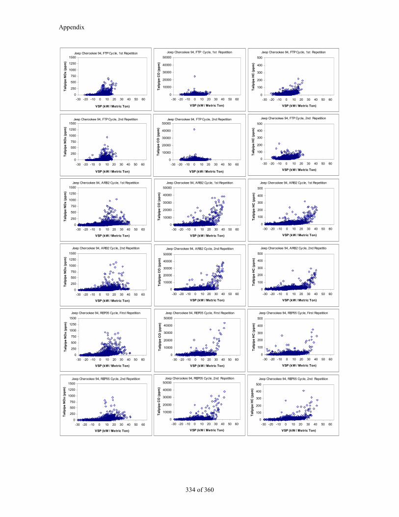
Appendix

334 of 360

Jeep Cherookee 94, FTP Cycle, 1st Repetition

0

250

500

750

1000

1250

1500

-30 -20 -10 0 10 20 30 40 50 60

VSP (kW / Metric Ton)

Tai

lpip

e N

Ox

(pp

m)

Jeep Cherookee 94, FTP Cycle, 1st Repetition

0

10000

20000

30000

40000

50000

-30 -20 -10 0 10 20 30 40 50 60

VSP (kW / Metric Ton)

Tai

lpip

e C

O (

pp

m)

Jeep Cherookee 94, FTP Cycle, 1st Repetition

0

100

200

300

400

500

-30 -20 -10 0 10 20 30 40 50 60

VSP (kW / Metric Ton)

Tai

lpip

e H

C (

pp

m)

Jeep Cherookee 94, FTP Cycle, 2nd Repetition

0

250

500

750

1000

1250

1500

-30 -20 -10 0 10 20 30 40 50 60

VSP (kW / Metric Ton)

Tai

lpip

e N

Ox

(pp

m)

Jeep Cherookee 94, FTP Cycle, 2nd Repetition

0

10000

20000

30000

40000

50000

-30 -20 -10 0 10 20 30 40 50 60

VSP (kW / Metric Ton)

Tai

lpip

e C

O (

pp

m)

Jeep Cherookee 94, FTP Cycle, 2nd Repetition

0

100

200

300

400

500

-30 -20 -10 0 10 20 30 40 50 60

VSP (kW / Metric Ton)

Tai

lpip

e H

C (

pp

m)

Jeep Cherookee 94, ARB2 Cycle, 1st Repetition

0

250

500

750

1000

1250

1500

-30 -20 -10 0 10 20 30 40 50 60

VSP (kW / Metric Ton)

Tai

lpip

e N

Ox

(pp

m)

Jeep Cherookee 94, ARB2 Cycle, 1st Repetition

0

10000

20000

30000

40000

50000

-30 -20 -10 0 10 20 30 40 50 60

VSP (kW / Metric Ton)

Tai

lpip

e C

O (

pp

m)

Jeep Cherookee 94, ARB2 Cycle, 1st Repetition

0

100

200

300

400

500

-30 -20 -10 0 10 20 30 40 50 60

VSP (kW / Metric Ton)

Tai

lpip

e H

C (

pp

m)

Jeep Cherookee 94, ARB2 Cycle, 2nd Repetition

0

250

500

750

1000

1250

1500

-30 -20 -10 0 10 20 30 40 50 60

VSP (kW / Metric Ton)

Tai

lpip

e N

Ox

(pp

m)

Jeep Cherookee 94, ARB2 Cycle, 2nd Repetition

0

10000

20000

30000

40000

50000

-30 -20 -10 0 10 20 30 40 50 60

VSP (kW / Metric Ton)

Tai

lpip

e C

O (

pp

m)

Jeep Cherookee 94, ARB2 Cycle, 2nd Repetitio

0

100

200

300

400

500

-30 -20 -10 0 10 20 30 40 50 60

VSP (kW / Metric Ton)

Tai

lpip

e H

C (

pp

m)

Jeep Cherookee 94, REP05 Cycle, First Repetition

0

250

500

750

1000

1250

1500

-30 -20 -10 0 10 20 30 40 50 60

VSP (kW / Metric Ton)

Tai

lpip

e N

Ox

(pp

m)

Jeep Cherookee 94, REP05 Cycle, First Repetition

0

10000

20000

30000

40000

50000

-30 -20 -10 0 10 20 30 40 50 60

VSP (kW / Metric Ton)

Tai

lpip

e C

O (

pp

m)

Jeep Cherookee 94, REP05 Cycle, First Repetition

0

100

200

300

400

500

-30 -20 -10 0 10 20 30 40 50 60

VSP (kW / Metric Ton)

Tai

lpip

e H

C (

pp

m)

Jeep Cherookee 94, REP05 Cycle, 2nd Repetition

0

250

500

750

1000

1250

1500

-30 -20 -10 0 10 20 30 40 50 60

VSP (kW / Metric Ton)

Tai

lpip

e N

Ox

(pp

m)

Jeep Cherookee 94, REP05 Cycle, 2nd Repetition

0

10000

20000

30000

40000

50000

-30 -20 -10 0 10 20 30 40 50 60

VSP (kW / Metric Ton)

Tai

lpip

e C

O (

pp

m)

Jeep Cherookee 94, REP05 Cycle, 2nd Repetition

0

100

200

300

400

500

-30 -20 -10 0 10 20 30 40 50 60

VSP (kW / Metric Ton)

Tai

lpip

e H

C (

pp

m)

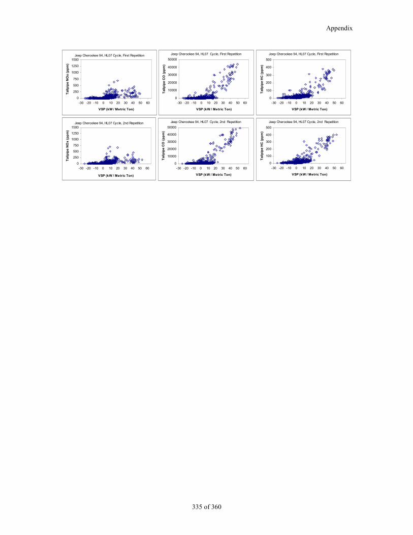
Appendix

335 of 360

Jeep Cherookee 94, HL07 Cycle, First Repetition

0

250

500

750

1000

1250

1500

-30 -20 -10 0 10 20 30 40 50 60

VSP (kW / Metric Ton)

Tai

lpip

e N

Ox

(pp

m)

Jeep Cherookee 94, HL07 Cycle, First Repetition

0

10000

20000

30000

40000

50000

-30 -20 -10 0 10 20 30 40 50 60

VSP (kW / Metric Ton)

Tai

lpip

e C

O (

pp

m)

Jeep Cherookee 94, HL07 Cycle, First Repetition

0

100

200

300

400

500

-30 -20 -10 0 10 20 30 40 50 60

VSP (kW / Metric Ton)

Tai

lpip

e H

C (

pp

m)

Jeep Cherookee 94, HL07 Cycle, 2nd Repetition

0

250

500

750

1000

1250

1500

-30 -20 -10 0 10 20 30 40 50 60

VSP (kW / Metric Ton)

Tai

lpip

e N

Ox

(pp

m)

Jeep Cherookee 94, HL07 Cycle, 2nd Repetition

0

10000

20000

30000

40000

50000

-30 -20 -10 0 10 20 30 40 50 60

VSP (kW / Metric Ton)

Tai

lpip

e C

O (

pp

m)

Jeep Cherookee 94, HL07 Cycle, 2nd Repetition

0

100

200

300

400

500

-30 -20 -10 0 10 20 30 40 50 60

VSP (kW / Metric Ton)

Tai

lpip

e H

C (

pp

m)

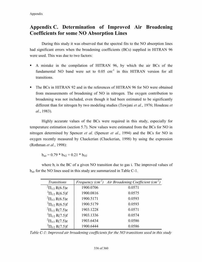
Appendix

336 of 360

Appendix C. Determination of Improved Air BroadeningCoefficients for some NO Absorption Lines

During this study it was observed that the spectral fits to the NO absorption lines

had significant errors when the broadening coefficients (BCs) supplied in HITRAN 96

were used. This was due to two factors:

A mistake in the compilation of HITRAN 96, by which the air BCs of the

fundamental NO band were set to 0.05 cm-1 in this HITRAN version for all

transitions.

The BCs in HITRAN 92 and in the references of HITRAN 96 for NO were obtained

from measurements of broadening of NO in nitrogen. The oxygen contribution to

broadening was not included, even though it had been estimated to be significantly

different than for nitrogen by two modeling studies (Tewjani et al., 1976; Houdeau et

al., 1983).

Highly accurate values of the BCs were required in this study, especially for

temperature estimation (section 5.7). New values were estimated from the BCs for NO in

nitrogen determined by Spencer et al. (Spencer et al., 1994) and the BCs for NO in

oxygen recently measured by Chackerian (Chackerian, 1998) by using the expression

(Rothman et al., 1998):

bair = 0.79 * bN2 + 0.21 * bO2

where bi is the BC of a given NO transition due to gas i. The improved values of

bair for the NO lines used in this study are summarized in Table C-1.

Transitions Frequency (cm-1) Air Broadening Coefficient (cm-1)2Π1/2 R(6.5)e 1900.0706 0.05712Π1/2 R(6.5)f 1900.0816 0.05752Π3/2 R(6.5)e 1900.5171 0.05932Π3/2 R(6.5)f 1900.5179 0.05932Π1/2 R(7.5)e 1903.1228 0.05712Π1/2 R(7.5)f 1903.1336 0.05742Π3/2 R(7.5)e 1903.6434 0.05862Π3/2 R(7.5)f 1900.6444 0.0586

Table C-1: Improved air broadening coefficients for the NO transitions used in this study

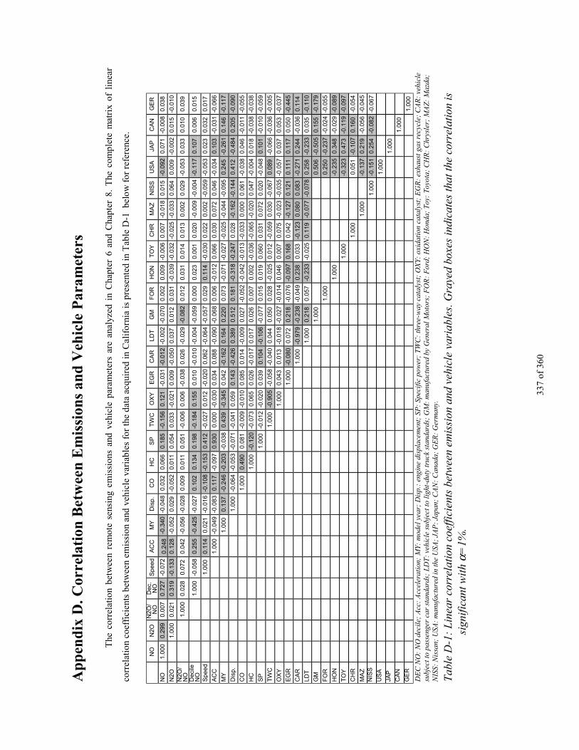
337

of 3

60

Ap

pen

dix

D. C

orre

lati

on B

etw

een

Em

issi

ons

and

Veh

icle

Par

amet

ers

The

cor

rela

tion

bet

wee

n re

mot

e se

nsin

g em

issi

ons

and

vehi

cle

para

met

ers

are

anal

yzed

in

Cha

pter

6 a

nd C

hapt

er 8

. T

he c

ompl

ete

mat

rix

of l

inea

r

corr

elat

ion

coef

fici

ents

bet

wee

n em

issi

on a

nd v

ehic

le v

aria

bles

for

the

data

acq

uire

d in

Cal

ifor

nia

is p

rese

nted

in T

able

D-1

bel

ow f

or r

efer

ence

.

NO

N2O

N2O

/N

OD

ec.

NO

Speed

AC

CM

YD

isp.

CO

HC

SP

TW

CO

XY

EG

RC

AR

LD

TG

MF

OR

HO

NT

OY

CH

RM

AZ

NIS

SU

SA

JAP

CA

NG

ER

NO

1.0

00

0.2

99

0.0

07

0.7

27

-0.0

72

0.2

48

-0.3

40

-0.0

48

0.0

32

0.0

66

0.1

85

-0.1

56

0.1

21

-0.0

31

-0.0

12

-0.0

02

-0.0

70

0.0

02

0.0

09

-0.0

06

0.0

07

-0.0

18

0.0

15

-0.0

92

0.0

71

-0.0

08

0.0

38

N2O

1.0

00

0.0

21

0.3

19

-0.1

33

0.1

28

-0.0

52

0.0

29

-0.0

52

0.0

11

0.0

54

0.0

33

-0.0

21

0.0

09

-0.0

50

0.0

37

0.0

12

0.0

31

-0.0

39

-0.0

32

-0.0

25

-0.0

33

0.0

64

0.0

09

-0.0

02

0.0

15

-0.0

10

N2O

/N

O1.0

00

0.0

28

0.0

72

0.0

42

-0.0

56

-0.0

28

0.0

09

0.0

11

0.0

51

-0.0

06

0.0

06

-0.0

38

0.0

26

-0.0

29

-0.0

82

0.0

12

0.0

31

0.0

14

0.0

13

0.0

02

0.0

29

-0.0

53

0.0

33

0.0

10

0.0

39

Deci

leN

O1.0

00

-0.0

58

0.2

55

-0.4

25

-0.0

27

0.1

02

0.1

34

0.1

98

-0.1

84

0.1

55

0.0

10

-0.0

10

-0.0

04

-0.0

59

0.0

00

0.0

23

0.0

01

0.0

20

-0.0

09

-0.0

04

-0.1

17

0.1

07

0.0

06

0.0

15

Speed

1.0

00

0.1

14

0.0

21

-0.0

16

-0.1

08

-0.1

53

0.4

12

-0.0

27

0.0

12

-0.0

20

0.0

62

-0.0

64

-0.0

57

0.0

29

0.1

14

-0.0

30

0.0

22

0.0

02

-0.0

59

-0.0

53

0.0

23

0.0

32

0.0

17

AC

C1.0

00

-0.0

49

-0.0

83

0.1

17

-0.0

97

0.9

30

0.0

00

-0.0

30

0.0

34

0.0

88

-0.0

90

-0.0

68

0.0

06

-0.0

12

0.0

66

0.0

30

0.0

72

0.0

46

-0.0

34

0.1

03

-0.0

31

-0.0

66

MY

1.0

00

0.1

37

-0.2

46

-0.2

03

-0.0

38

0.4

39

-0.3

45

0.0

42

-0.1

62

0.1

64

0.2

20

0.0

73

-0.0

71

-0.0

27

-0.0

25

-0.0

44

-0.0

95

0.2

45

-0.2

61

0.1

46

-0.1

17

Dis

p.

1.0

00

-0.0

64

-0.0

53

-0.0

71

-0.0

41

0.0

59

0.1

43

-0.4

26

0.3

89

0.5

12

0.1

81

-0.3

18

-0.2

47

0.0

28

-0.1

62

-0.1

44

0.4

12

-0.4

84

0.2

05

-0.0

90

CO

1.0

00

0.4

90

0.0

81

-0.0

09

-0.0

10

0.0

85

0.0

14

-0.0

09

0.0

27

-0.0

52

-0.0

42

-0.0

13

-0.0

33

0.0

00

0.0

61

-0.0

38

0.0

46

-0.0

11

-0.0

55

HC

1.0

00

-0.1

20

-0.0

73

0.0

65

0.0

26

-0.0

17

0.0

17

0.0

26

0.0

07

0.0

02

-0.0

36

-0.0

65

-0.0

20

0.0

47

-0.0

04

0.0

18

-0.0

38

-0.0

38

SP

1.0

00

-0.0

12

-0.0

20

0.0

39

0.1

04

-0.1

06

-0.0

77

0.0

15

0.0

19

0.0

60

0.0

31

0.0

72

0.0

20

-0.0

48

0.1

01

-0.0

10

-0.0

59

TW

C1.0

00

-0.9

05

-0.0

58

-0.0

40

0.0

44

0.0

50

0.0

28

-0.0

25

0.0

12

-0.0

59

0.0

30

-0.0

67

0.0

89

-0.0

66

-0.0

36

-0.0

05

OX

Y1.0

00

0.0

43

0.0

13

-0.0

18

-0.0

27

-0.0

14

0.0

46

0.0

07

0.0

75

-0.0

23

-0.0

35

-0.0

57

0.0

37

0.0

53

-0.0

37

EG

R1.0

00

-0.0

80

0.0

72

0.2

18

-0.0

76

-0.0

97

0.1

68

0.0

42

-0.1

27

0.1

21

0.1

11

0.1

17

0.0

50

-0.4

45

CA

R1.0

00

-0.9

79

-0.2

38

-0.0

49

0.2

38

0.0

33

-0.1

23

0.0

80

0.0

83

-0.2

71

0.2

44

-0.0

36

0.1

14

LD

T1.0

00

0.2

18

0.0

57

-0.2

33

-0.0

25

0.1

19

-0.0

77

-0.0

78

0.2

58

-0.2

33

0.0

35

-0.1

10

GM

1.0

00

0.5

06

-0.5

05

0.1

55

-0.1

79

FO

R1.0

00

0.2

50

-0.2

37

-0.0

24

-0.0

55

HO

N1.0

00

-0.2

35

0.3

48

-0.0

29

-0.0

89

TO

Y1.0

00

-0.3

23

0.4

73

-0.1

19

-0.0

97

CH

R1.0

00

0.0

51

-0.1

07

0.1

60

-0.0

54

MA

Z1.0

00

-0.1

37

0.2

19

-0.0

56

-0.0

45

NIS

S1.0

00

-0.1

51

0.2

54

-0.0

82

-0.0

67

US

A1.0

00

JAP

1.0

00

CA

N1.0

00

GE

R1.0

00

DE

C N

O:

NO

dec

ile;

Acc

: A

ccel

erat

ion;

MY:

mod

el y

ear;

Dis

p.:

engi

ne d

ispl

acem

ent;

SP

: Sp

ecif

ic p

ower

; T

WC

: th

ree-

way

cat

alys

t; O

XY:

oxi

dati

on c

atal

yst;

EG

R:

exha

ust g

as r

ecyc

le;

CA

R:

vehi

cle

subj

ect t

o pa

ssen

ger

car

stan

dard

s; L

DT

: ve

hicl

e su

bjec

t to

ligh

t-du

ty tr

uck

stan

dard

s; G

M:

man

ufac

ture

d by

Gen

eral

Mot

ors;

FO

R:

For

d; H

ON

: H

onda

; T

oy:

Toyo

ta;

CH

R:

Chr

ysle

r; M

AZ

: M

azda

;N

ISS:

Nis

san;

USA

: m

anuf

actu

red

in th

e U

SA;

JAP

: Ja

pan;

CA

N:

Can

ada;

GE

R:

Ger

man

y.

Tab

le D

-1:

Lin

ear

corr

elat

ion

coef

fici

ents

bet

wee

n em

issi

on a

nd v

ehic

le v

aria

bles

. Gra

yed

boxe

s in

dica

tes

that

the

corr

elat

ion

issi

gnif

ican

t wit

h α=

1%.

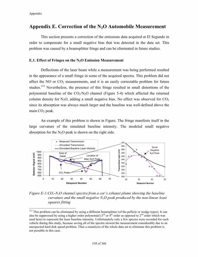
Appendix

338 of 360

Appendix E. Correction of the N2O Automobile Measurement

This section presents a correction of the emissions data acquired at El Segundo in

order to compensate for a small negative bias that was detected in the data set. This

problem was caused by a beamsplitter fringe and can be eliminated in future studies.

E.1. Effect of Fringes on the N2O Emission Measurement

Deflections of the laser beam while a measurement was being performed resulted

in the appearance of a small fringe in some of the acquired spectra. This problem did not

affect the NO or CO2 measurements, and it is an easily correctable problem for future

studies.313 Nevertheless, the presence of this fringe resulted in small distortions of the

polynomial baseline of the CO2/N2O channel (Figure 5-4) which affected the returned

column density for N2O, adding a small negative bias. No effect was observed for CO2

since its absorption was always much larger and the baseline was well-defined above the

main CO2 peak.

An example of this problem is shown in Figure. The fringe manifests itself in the

large curvature of the simulated baseline intensity. The modeled small negative

absorption for the N2O peak is shown on the right side.

600650700750800850900950

1000

0 10 20 30 40 50 60 70

Datapoint Number

Det

ecto

r S

ign

al (

mV

)

Measured Transmission

Simulated Transmission

Simulated Baseline Laser Intensity

Area ofDetail

CO2 Peaks

Location of

Main N2O Peak

820

825

830

835

840

845

850

855

860

865

870

20 25 30 35

Datapoint Number

Tra

nsm

itte

d L

igh

t (m

V)

SmallNegative

N2O Peak

Figure E-1:CO2-N2O channel spectra from a car’s exhaust plume showing the baselinecurvature and the small negative N2O peak produced by the non-linear leastsquares fitting

313 This problem can be eliminated by using a different beamsplitter (of the pellicle or wedge types). It canalso be suppressed by using a higher order polynomial (3rd or 4th order as opposed to 2nd order which wasused here) to represent the laser baseline intensity. Unfortunately only a few spectra were recorded for eachvehicle during this study, because saving all of the spectra slowed the measurement considerably due to anunexpected hard disk speed problem. Thus a reanalysis of the whole data set to eliminate this problem isnot possible in this case.

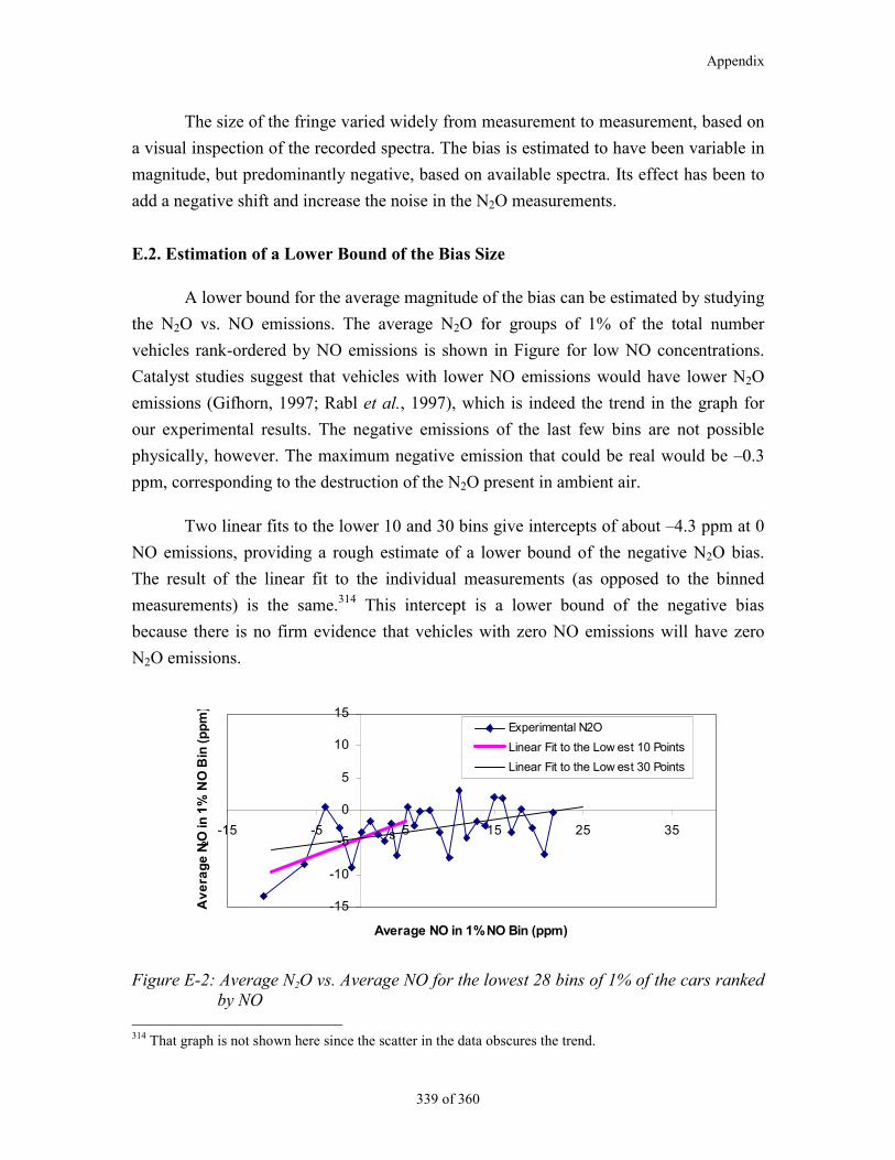
Appendix

339 of 360

The size of the fringe varied widely from measurement to measurement, based on

a visual inspection of the recorded spectra. The bias is estimated to have been variable in

magnitude, but predominantly negative, based on available spectra. Its effect has been to

add a negative shift and increase the noise in the N2O measurements.

E.2. Estimation of a Lower Bound of the Bias Size

A lower bound for the average magnitude of the bias can be estimated by studying

the N2O vs. NO emissions. The average N2O for groups of 1% of the total number

vehicles rank-ordered by NO emissions is shown in Figure for low NO concentrations.

Catalyst studies suggest that vehicles with lower NO emissions would have lower N2O

emissions (Gifhorn, 1997; Rabl et al., 1997), which is indeed the trend in the graph for

our experimental results. The negative emissions of the last few bins are not possible

physically, however. The maximum negative emission that could be real would be –0.3

ppm, corresponding to the destruction of the N2O present in ambient air.

Two linear fits to the lower 10 and 30 bins give intercepts of about –4.3 ppm at 0

NO emissions, providing a rough estimate of a lower bound of the negative N2O bias.

The result of the linear fit to the individual measurements (as opposed to the binned

measurements) is the same.314 This intercept is a lower bound of the negative bias

because there is no firm evidence that vehicles with zero NO emissions will have zero

N2O emissions.

-15

-10

-5

0

5

10

15

-15 -5 5 15 25 35

Average NO in 1% NO Bin (ppm)

Av

era

ge

N2O

in 1

% N

O B

in (

pp

m)

Experimental N2O

Linear Fit to the Low est 10 Points

Linear Fit to the Low est 30 Points

s

Figure E-2: Average N2O vs. Average NO for the lowest 28 bins of 1% of the cars rankedby NO

314 That graph is not shown here since the scatter in the data obscures the trend.

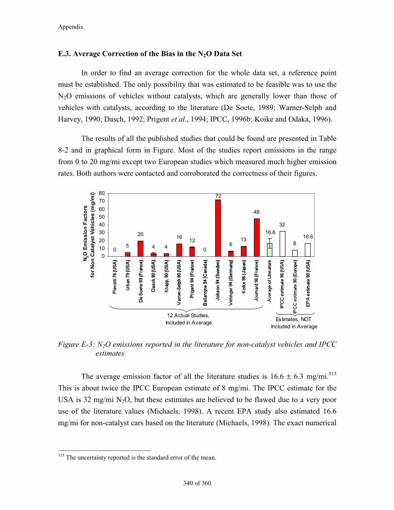
Appendix

340 of 360

E.3. Average Correction of the Bias in the N2O Data Set

In order to find an average correction for the whole data set, a reference point

must be established. The only possibility that was estimated to be feasible was to use the

N2O emissions of vehicles without catalysts, which are generally lower than those of

vehicles with catalysts, according to the literature (De Soete, 1989; Warner-Selph and

Harvey, 1990; Dasch, 1992; Prigent et al., 1994; IPCC, 1996b; Koike and Odaka, 1996).

The results of all the published studies that could be found are presented in Table

8-2 and in graphical form in Figure. Most of the studies report emissions in the range

from 0 to 20 mg/mi except two European studies which measured much higher emission

rates. Both authors were contacted and corroborated the correctness of their figures.

05

20

4 4

1612

06

13

48

32

816.6

72

16.6

0

10

20

30

40

50

60

70

80

N2O

Em

issi

on

Fac

tors

fo

r N

on

Cat

alys

t V

ehic

les

(mg

/mi)

12 Actual Studies, Included in Average

Estimates, NOT Included in Average

Figure E-3: N2O emissions reported in the literature for non-catalyst vehicles and IPCCestimates

The average emission factor of all the literature studies is 16.6 ± 6.3 mg/mi.315

This is about twice the IPCC European estimate of 8 mg/mi. The IPCC estimate for the

USA is 32 mg/mi N2O, but these estimates are believed to be flawed due to a very poor

use of the literature values (Michaels, 1998). A recent EPA study also estimated 16.6

mg/mi for non-catalyst cars based on the literature (Michaels, 1998). The exact numerical

315 The uncertainty reported is the standard error of the mean.

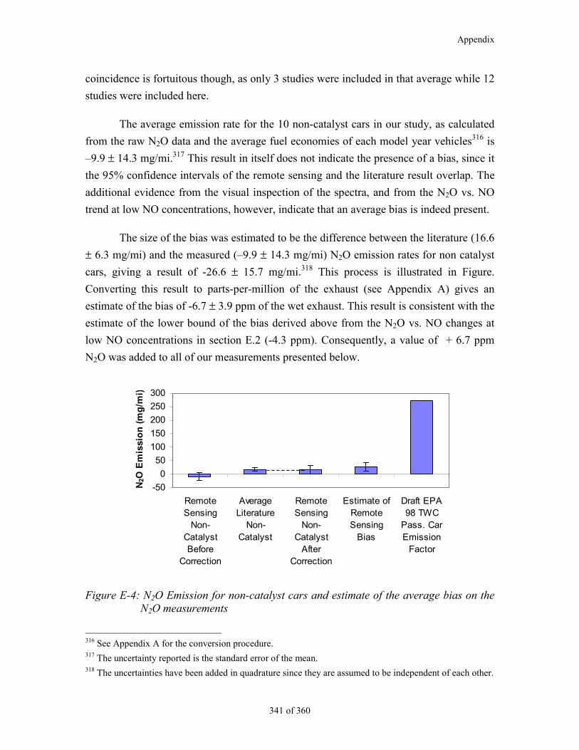
Appendix

341 of 360

coincidence is fortuitous though, as only 3 studies were included in that average while 12

studies were included here.

The average emission rate for the 10 non-catalyst cars in our study, as calculated

from the raw N2O data and the average fuel economies of each model year vehicles316 is

–9.9 ± 14.3 mg/mi.317 This result in itself does not indicate the presence of a bias, since it

the 95% confidence intervals of the remote sensing and the literature result overlap. The

additional evidence from the visual inspection of the spectra, and from the N2O vs. NO

trend at low NO concentrations, however, indicate that an average bias is indeed present.

The size of the bias was estimated to be the difference between the literature (16.6

± 6.3 mg/mi) and the measured (–9.9 ± 14.3 mg/mi) N2O emission rates for non catalyst

cars, giving a result of -26.6 ± 15.7 mg/mi.318 This process is illustrated in Figure.

Converting this result to parts-per-million of the exhaust (see Appendix A) gives an

estimate of the bias of -6.7 ± 3.9 ppm of the wet exhaust. This result is consistent with the

estimate of the lower bound of the bias derived above from the N2O vs. NO changes at

low NO concentrations in section E.2 (-4.3 ppm). Consequently, a value of + 6.7 ppm

N2O was added to all of our measurements presented below.

-50

0

50

100

150

200

250

300

RemoteSensing

Non-CatalystBefore

Correction

AverageLiterature

Non-Catalyst

RemoteSensing

Non-Catalyst

AfterCorrection

Estimate ofRemoteSensing

Bias

Draft EPA98 TWC

Pass. CarEmission

Factor

N2O

Em

issi

on

(m

g/m

i)

Figure E-4: N2O Emission for non-catalyst cars and estimate of the average bias on theN2O measurements

316 See Appendix A for the conversion procedure.317 The uncertainty reported is the standard error of the mean.318 The uncertainties have been added in quadrature since they are assumed to be independent of each other.

Appendix

342 of 360

An independent check on the bias correction procedure was provided by the N2O

measurements on the prototype ultra-low emissions vehicle (ULEV) described in section

5.4.2, which are not included in the previous analysis. The average of the 16 N2O

readings corresponding to NO values within ±10 ppm yielded an average of 2.2 ± 1.12

ppm N2O (after bias correction). This is very similar to the average level of the vehicles

in our data set which had similarly low NO emissions (2.4 ppm).

The correction deduced here is significant319, and some uncertainty remains on the

absolute values of our N2O remote sensing results. It was implemented due the unique

nature of this data set, and after realizing that all the trends of N2O emissions described in

the following sections (with emission control technology, vehicle age, type of vehicle,

speed, acceleration, and NO emissions) were very similar to those described in the

literature. It is impossible that all those trends will be matched by chance, and this

indicates that while there was a systematic negative bias in this particular measurement,

the measured values do bear a relationship with the N2O emission level of the vehicle.

319 Even though the correction is significant when compared with the average value of the data set, it issmall compared to the range of emission values that were observed and to the some of the emission factorsproposed for vehicles with three-way catalysts, as shown in Figure.

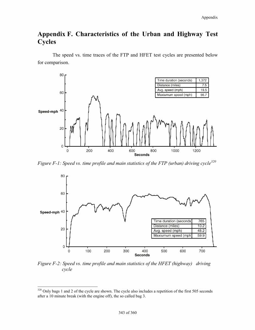
Appendix

343 of 360

Appendix F. Characteristics of the Urban and Highway TestCycles

The speed vs. time traces of the FTP and HFET test cycles are presented below

for comparison.

Figure F-1: Speed vs. time profile and main statistics of the FTP (urban) driving cycle320

Figure F-2: Speed vs. time profile and main statistics of the HFET (highway) drivingcycle

320 Only bags 1 and 2 of the cycle are shown. The cycle also includes a repetition of the first 505 secondsafter a 10 minute break (with the engine off), the so called bag 3.

344 of 360

Ahmed, S. R. and W. Baumert (1979). The Structure of Wake Flow Behind Road Vehicles. Aerodynamicsof Transportation. New York, NY, ASME.

Allen, M. G. (1998). “Diode Laser Absorption Sensors for Gas-Dynamic and Combustion Flows.”Measurement Science and Technology 9: 545-562.

Allen, M. G. and W. J. Kessler (1996). “Simultaneous Water Vapor Concentration and TemperatureMeasurements Using 1.31-µm Diode Lasers.” AIAA Journal 34(3): 483-488.

An, F., Ross, M. (1996). “A Simple Physical Model for High Power Enrichment Emissions.” Journal of theAir and Waste Management Association 46: 216-223.

An, F. and G. Scora (1997). "Characterization and Modeling of Vehicular Unburned HydrocarbonEmissions." Seventh CRC On-Road Vehicle Emissions Workshop, San Diego, California.

Ando, A. W., W. Harrington and V. McConell (1998). “Estimating Full IM240 Emissions from PartialTests Results: Evidence from Arizona.” Resources for the Future, Discussion Paper 98-24, Washington,DC.

Arroyo, M. P. and R. K. Hanson (1993). “Absorption Measurements of Water-Vapor Concentration,Temperature, and Line-Shape Parameters Using a Tunable InGaAsP Diode Laser.” Applied Optics 32(30):6104-6116.

Arroyo, M. P., S. Langlois and R. K. Hanson (1994). “Diode-Laser Absorption Technique forSimultaneous Measurements of Multiple Gasdynamic Parameters in High-Speed Flows Containing WaterVapor.” Applied Optics 33(15): 3296-3307.

Atkinson, C. C.M., N.N., T. W. Long and E. L. Hanzevack (1998). "Neural Network-Based VehicleEmissions Modeling for Inventory Applications-An Update on Virtual Sensing." Eighth CRC On-RoadVehicle Emissions Workshop, San Diego, California.

Atkinson, C. M., N. N. Clark and D. W. Lyons (1996). "An Estimation of the Comparative Contribution ofHeavy-Duty Diesel Buses and Trucks to Mobile Source Emissions." Sixth CRC On-Road VehicleEmissions Workshop, San Diego, California.

Baer, D. S., R. K. Hanson, M. E. Newfield and N. K. J. M. Gopaul (1994). “Multiplexed Diode-LaserSensor System for Simultaneous H2O, O2, and Temperature Measurements.” Optical Letters 19(22): 1900-1902.

Baer, D. S., V. Nagali, F. E.R. and R. K. Hanson (1996). “Scanned- and Fixed-Wavelength AbsorptionDiagnostics for Combustion Measurements Using Multiplexed Diode Lasers.” AIAA Journal 34(3): 489-493.

Baker, R., J. McFarland, S. Kishan, R. Klausmeier, D. Grubbe and F. Cox (1997). "Use of Remote SensingDevices to Identify Clean Vehicles for Exemption from I/M Testing." Seventh CRC On-Road VehicleEmissions Workshop, San Diego, California.

Ballantyne, V. F., P. Howes and L. Stephanson (1994). “Nitrous Oxide Emissions from Light DutyVehicles.” Society of Automotive Engineers Paper 940304.

Barnard, R. H. (1996). Road Vehicle Aerodynamic Design: An Introduction. Addison Wesley LongmanLtd., Harlow, England.

Barrett, R. (1998). "Colorado's I/M Program." 1998 Summer Symposium of the EPA Center on AirborneOrganics, Dedham, MA.

Barth, M. and J. Norbeck (1997). "NCHRP Project 25-11: The Development of a Comprehensive ModalEmissions Model." Seventh CRC On-Road Vehicle Emissions Workshop, San Diego, California.

Barth, M., J. Norbeck and M. Ross (1998). "Recent Progress on NCHRP Project 25-11: The Developmentof a Comprehensive Modal Emissions Model." Eighth CRC On-Road Vehicle Emissions Workshop, SanDiego, California.

Barton, P. (1998). Environment Canada. Personal Communication.

References

345 of 360

Barton, P. and J. Simpson (1994). “The Effects of Aged Catalysts and Cold Ambient Temperatures onNitrous Oxide Emissions. (Unpublished).” Technology Development Directorate, Environment Canada,MSED #94-21, Ottawa, Canada.

Batchelor, G. (1973). Introduction to Fluid Dynamics. Cambridge University Press, .

Bauer, H. (1996). Bosch Automotive Handbook, 4th Ed. Robert Bentley Publishers, Cambridge,Massachusetts.

Baum, M. M. (1997). "Characterizing and Analyzing Components of Vehicle Exhaust Emissions by UVSpectroscopy." World Car Conference, Riverside, CA.

Beardsley, M. (1998). Emission Inventory Group, U.S. EPA. Personal Communication.

Beaton, S. P., G. A. Bishop and D. H. Stedman (1992). “Emission characteristics of Mexico City vehicles.”Journal of the Air & Waste Management Association 42: 1424-9.

Beaton, S. P., G. A. Bishop, Y. Zhang, L. L. Ashbaugh, D. R. Lawson and D. H. Stedman (1995). “On-Road Vehicle Emissions: Regulations, Costs, and Benefits.” Science 268: 991.

Beer, J. M. and N. A. Chigier (1972). Combustion Aerodynamics. Applied Science Publishers Ltd.,London.

Berens, D., H. H. Haskew and R. Orteca (1997). "FTP Emissions from 1991-93 MY in Use Vehicles."Seventh CRC On-Road Vehicle Emissions Workshop, San Diego, California.

Berges, M. G., R. M. Hofmann, D. Scharfe and P. J. Crutzen (1993). “Nitrous Oxide Emissions from MotorVehicles in Tunnels and Their Global Extrapolation.” Journal of Geophysical Research 98(D10): 18527-18531.

Bishop, G. A., B. R. Hutton and D. H. Stedman (1996a). "Design and Operation of a Public InformationSystem for Voluntary Emissions Reduction Using RSD Technology and Its Operational Test." Sixth CRCWorkshop on Vehicle Emissions, San Diego, California.

Bishop, G. A., S. E. McLaren and D. H. Stedman, Pierson, W.R.,Zweidinger, R.B., Ray, W.D. (1996b).“Method Comparisons of Vehicle Emissions Measurements in the Fort McHenry and Tuscarora MountainTunnels.” Atmospheric Environment 30 no12: 2307-16.

Bishop, G. A., J. R. Starkey and A. Ihlenfeldt (1989). “IR long-path photometry: a remote sensing tool forautomobile emissions.” Analytical Chemistry 61: 671A.

Bishop, G. A. and D. H. Stedman (1990). “On-road carbon monoxide emission measurement comparisonsfor the 1988-1989 Colorado oxy-fuels program.” Environmental Science & Technology 24: 843-7.

Bishop, G. A. and D. H. Stedman (1996c). “Measuring the Emissions of Passing Cars.” Accounts ofChemical Research 29(10): 489.

Bishop, G. A., D. H. Stedman and L. Ashbaugh (1996d). “Motor Vehicle Emissions Variability.” J. AirWaste Manage. Assoc. 46: 667-675.

Bishop, G. A., D. H. Stedman and J. de la Garza Castro (1997). “On-road remote sensing of vehicleemissions in Mexico.” Environmental Science & Technology 31: 3505-.

Bishop, G. A., D. H. Stedman and T. Jessop (1992). “Infrared emission and remote sensing.” Journal of theAir & Waste Management Association 42: 695-7.

Bishop, G. A., D. H. Stedman and J. E. Peterson (1993). “A cost-effectiveness study of carbon monoxideemissions reduction utilizing remote sensing.” Air & Waste 43: 978-88.

Bishop, G. A., Y. Zhang and S. E. McLaren, Guenther, P.L., Beaton, S.P., Peterson, J.E., Stedman, D.H.,Pierson, W.R., Knapp, K.T., Zweidinger, R.B., Duncan, J.W., McArver, A.Q., Groblicki, P.J., Day, J.F.(1994). “Enhancements of Remote Sensing for Vehicle Emissions in Tunnels.” Journal of the Air andWaste Management Association 44(2): 169-175.

References

346 of 360

Bouwman, A. F., K. W. Van der Hoek and J. G. J. Olivier (1995). “Uncertainties in the Global SourceDistribution of Nitrous Oxide.” Journal of Geophysical Research 100(D2): 2785-2800.

Bowman, C. T. (1992). "Control of Combustion-Generated Nitrogen Oxide Emissions: Technology Drivenby Regulation." 24th Symposium (International) on Combustion, The Combustion Institute, Pittsburgh.

Braddock, J. N. (1981). “Impact of Low Ambient Temperature on 3-Way Catalyst Car Emissions.” Societyof Automotive Engineers Paper 810280.

Brown, J. E. (1997). Acurex, Inc. Personal Communication.

Cackette, T. (1998). "The Cost of Emission Controls. Motor Vehicles and Fuels: Two Case Studies." 1998Summer Symposium of the EPA Center on Airborne Organics, Dedham, Massachusetts.

Cadle, S. H., R. A. Gorse and T. C. Belian (1997). “Real-world vehicle emissions: a summary of the SixthCoordinating Research Council On-Road Vehicle Emissions Workshop. (San Diego, Calif., Mar. 18-20,1996).” Journal of the Air & Waste Management Association (1995) 47: 426-38.

Cadle, S. H., R. A. Gorse and T. C. Belian (1998). “Real-world vehicle emissions: a summary of theSeventh Coordinating Research Council On-Road Vehicle Emissions Workshop. (San Diego, Calif., Apr.9-11, 1997).” Journal of the Air & Waste Management Association (1995) 48: 174-85.

Cadle, S. H. and P. A. Mulawa (1980). “Low Molecular Weight Aliphatic Amines in Exhaust fromCatalyst-Equipped Cars.” Environmental Science and Technology 14(6): 718-723.

Cadle, S. H. and R. D. Stephens (1994). “Remote sensing of vehicle exhaust emissions.” EnvironmentalScience & Technology 28: 258A-.

Calvert, J. G., J. B. Heywood, R. F. Sawyer and J. H. Seinfeld (1993). “Achieving Acceptable Air Quality:Some Reflections on Controlling Vehicle Emissions.” Science 261: 37-45.

Cant, N. W., D. E. Angove and D. C. Chambers (1998). “Nitrous Oxide Formation During the Reaction ofSimulated Exhaust Streams over Rhodium, Platinum, and Palladium Catalysts.” Applied Catalysis B:Environmental 17: 63-73.

CARB (1996a). “California exhaust Emission Standards and Test Procedures for 1988 and SubsequentModel Passenger Cars, Light-Duty Trucks, and Medium-Duty Vehicles.” Mobile Source Division,California Air Resources Board, Sacramento, California.

CARB (1996b). “Low-Emission Vehicle and Zero-Emission Vehicle Program Review.” Mobile SourceDivision, California Air Resources Board, Sacramento, California.

CARB (1997a). “Draft Preliminary Staff Report: Proposed Amendments to California's Low-EmissionVehicle Regulations "LEV II".” Mobile Source Division, California Air Resources Board, El Monte,California.

CARB (1997b). "Proposed Amendments to Exhaust, Evaporative, and ORVR Emission Standards." LEV IIWorkshop, El Monte, California, Mobile Source Division, California Air Resources Board.

CARB (1998a). “EMFACX Workshop Reports.” Mobile Source Division, California Air ResourcesBoard, Sacramento, California.

CARB (1998b). “News Release: Air Board Continues California's World Leadership in Auto EmissionStandards.” California Air Resources Board, Sacramento, California.

CARB (1998c). “Proposed California Exhaust Emission Standards and Test Procedures for 2001 andSubsequent Model Passenger Cars, Light-Duty Trucks, and Medium Duty Vehicles.” California AirResources Board, El Monte, California.

Carduner, K. R., A. D. Colvin and R. Y. Leong, Schueltze, D., Mackay, G.I., Karecki, D.R., Schiff, H.I.(1992). “Application of Tunable Diode Laser Spectroscopy to the Real-Time Analysis of Engine OilEconomy.” Environmental Science and Technology 26(5): 930-934.

Carlson, T. R. and T. C. Austin (1997). “Development of Speed Correction Cycles.” Sierra Research, Inc.,SR97-04-01, Sacramento, California.

References

347 of 360

Cass, G. (1998). California Institute of Technology. Personal Communication.

Chackerian, C. (1998). NASA Ames Research Center. Personal Communication.

Chang, A. Y., M. D. Dirosa, D. F. Davidson and R. K. Hanson (1991). “Rapid Tuning CW LaserTechnique for Measurements of Gas Velocity, Temperature, Pressure, Density, and Mass Flux Using NO.”Applied Optics 30(21): 3011-3022.

Chen, G., T. J. Prochnau and D. L. Hofeldt (1996). “Feasibility of Remote Sensing of Particulate Emissionsfrom Heady-Duty Vehicles.” Society of Automotive Engineering Paper 960250.

Cicero-Fernandez, P. and J. R. Long (1995). "Grades and Other Loads Effects on On-Road Emissions: AnOn-Board Analyzer Study." Fifth CRC On-Road Vehicle Emissions Workshop, San Diego, California.

Cicero-Fernandez, P. and J. R. Long (1996). "Assessment of Commuting Under Grade Loads and RampMetering: Preliminary On-Road Emissions Findings." World Car Conference '96, University of Californiaat Riverside.

Clark, N. N. and D. W. Lyons (1996). "Driving Routes (or Icon Tests) for Heavy-Duty Truck EmissionsMeasurement." Sixth CRC On-Road Vehicle Emissions Workshop, San Diego, California.

Clark, N. N. and D. W. Lyons (1997). "Emissions from CNG and Diesel Refuse Haulers Using Six EngineTypes in New York City." Seventh CRC On-Road Vehicle Emissions Workshop, San Diego, California.

Clark, N. N., R. D. Nine and J. J. Daley, Atkinson, C.M., Peerenboom, W.H., Suski, V.A. (1998). "Heavy-Duty Truck Emissions: Vehicle Activity, Driving Routes, and NO2/NO Ratios." Eighth CRC On-Road

Vehicle Emissions Workshop, San Diego, California.

Clifford, M. J., R. Clarke and S. B. Riffat. (1997). “Local Aspects of Vehicular Air Pollution.” AtmosphericEnvironment 31(2): 271-276.

Cohen, J. P. and A. M. Noda (1995). “Auto/Oil Air Quality Improvement Research Program: Descriptionof Phase II Working Data Set.” Systems Applications International, SYSAPP-95/048, San Rafael,California.

Countess, R. and L. Cohen (1997). "Evaluation of Utilizing Remote Sensing to Monitor Tailpipe Emissionsfrom Heavy-Duty Vehicles." Seventh CRC On-Road Vehicle Emissions Workshop, San Diego, California.

Countess, R., L. Cohen and S. J. Countess, Bishop, G.A., Stedman, D.H. (1998). "Remote Sensing ofHeavy-Duty Diesel Truck Exhaust." Eighth CRC On-Road Vehicle Emissions Workshop, San Diego,California.

Dasch, J. M. (1992). “Nitrous oxide emissions from vehicles.” Journal of the Air & Waste ManagementAssociation 42(1): 63-67.

Davis, S. C. (1997). “Transportation Energy Data Book: Edition 17.” Oak Ridge National Laboratory,ORNL-6919, .

de Nevers, N. (1995). Air Pollution Control Engineering. McGraw-Hill, Inc., New York.

De Soete, G. (1989). “Updated Evaluation of Nitrous Oxide Emissions from Industrial Fossil FuelCombustion. Draft final report for the European Atomic Energy Community.” Institut Francais du Petrole,IFP 37-559, Rueil-Malmaison, France.

DeFries, T. (1997). Radian International LLC. Personal Communication.

DeFries, T. H. and H. J. Williamson (1997). “Methodology for Estimating California Fleet FTPEmissions.” Radian International, RCN 800916.01, Austin, Texas.

DiDomenico, J., J. Johnson and J. Webster, Rendahl, C.S. (1997). "Preliminary Results from Cold StartSensor Testing." Seventh CRC On-Road Vehicle Emissions Workshop, San Diego, California.

Dreher, D. B. and R. A. Harley (1998). “A Fuel-Based Inventory for Heavy-Duty Diesel Truck Emissions.”Journal of the Air and Waste Management Association 48: 352-358.

References

348 of 360

Eckbreth, A. C. (1981). "Recent Advances in Laser Diagnostics for Temperature and Species Concentrationin Combustion." Eighteenth Symposium (International) on Combustion, The Combustion Institute.

Ellerman, A. D. and A. Decaux (1998). “Analysis of Post-Kyoto CO2 Emissions Trading Using Marginal

Abatement Curves.” MIT Joint Program on the Science and Policy of Global Change, 40, .

Emmelman, H. J. and W. H. Hucho (1998). Performance of Cars and Light Trucks. Aerodynamics of RoadVehicles, 4th Ed. W. H. Hucho. Warrendale, Pennsylvania, Society of Automotive Engineers, Inc.

Environment Canada (1998). “News Release: Low Sulfur Gasoline Will Improve Health of Canadians.” ,Ottawa, Canada.

ES&T (1998). “Automakers Call for Low-Sulfur Fuel Sales.” Environmental Science and Technology32(15): 352A.

Eskridge, R. E., Petersen, W.B., Rao, S.T. (1991). “Turbulent Diffusion Behind Vehicles: Effect of TrafficSpeed on Pollutant Concentrations.” Journal of the Air and Waste Management Association 41: 312-317.

Flagan, R. C. and J. H. Seinfeld (1988). Fundamentals of Air Pollution Engineering. Prentice-Hall,Englewood Cliffs, N.J.

Fleiss, J. L. (1983). Statistical Methods for Rates and Proportions. John Wiley & Sons, Inc., New York,NY.

Fraser, M. P. and G. R. Cass (1998). “Detection of Excess Ammonia Emissions from In-Use Vehicles andthe Implications for Fine Particle Control.” Environmental Science and Technology 32: 1053-57.

Fujita, E. M., B. E. Croes and C. L. Bennett (1992). “Comparison of emission inventory and ambientconcentration ratios of CO, NMOG, and NOx in California's South Coast Air Basin.” Journal of the Air &Waste Management Association 42: 264-76.

Fujita, E. M., Z. Lu and L. H. Sheetz, Sagebiel, J.C., Zielinska, B. (1996). "Determination of MobileSource Emission Source Fraction using Ambient Field Measurements." Sixth CRC On-Road VehicleEmissions Workshop, San Diego, CA.

Fujita, E. M., J. G. Watson and J. C. Chow, Lu, Z. (1994). “Validation of the Chemical Mass BalanceReceptor Model Applied to Hydrocarbon Source Apportionment in the Southern California Air QualityStudy.” Environmental Science and Technology 28: 1633-1649.

Gammariello, R. and J. Long (1996). "Development of Unified Correction Cycles." Sixth CRC On-RoadVehicle Emissions Workshop, San Diego, California.

Gautam, M., D. Gupta and S. Popuri, Lyons, D.W. (1997). "Speciation and Reactivities of Diesel ExhaustEmissions." Seventh CRC On-Road Vehicle Emissions Workshop, San Diego, California.

Gertler, A., J. Sagebiel and W. Dippel (1997). "Results of the High Exhaust Emitters Project: SiteCharacterization, Selection, Feasibility Study." Seventh CRC On-Road Vehicle Emissions Workshop, SanDiego, California.

Gertler, A. W., J. C. Sagebiel and W. A. Dippel, Gillies, J.A., Gofa, F., O'Connor, C.M. (1998)."Comparison of the 1995 and 1996 Emissions at the Los Angeles Sepulveda Tunnel Including the Impactof California Phase 2 RFG." Eighth CRC On-Road Vehicle Emissions Workshop, San Diego, CA.

Gifhorn, A. (1997). “Einfluss der Abgas-zusammensetzug auf die N2O-Konvertierung an einem

Dreiwegekatalysator mit Pd/Rh-Beschichtung.” Fortschritt-Berichte VDI 12(337).

Gifhorn, A., H.-P. Rabl and R. Meyer-Pitroff (1997). "The Production of N2O over Three-Way Catalysts."

World Car Conference '97, Riverside, California.

Glover, E. L. and W. B. Clemens (1991). “Identifying Excess Emitters with Remote Sensing Devices: APreliminary Analysis.” Society of Automotive Engineers Paper 911672.

Good, D. (1998). US EPA Office of Mobile Sources. Personal Communication.

References

349 of 360

Graboski, M. S., J. Yanowitz and R. L. McCormick (1998). "In-Use Emissions from Heavy-Duty VehiclesOperating in the Colorado Northern Front Range Area." Eighth CRC On-Road Vehicle EmissionsWorkshop, San Diego, California.

Guensler, R., W. Bachman and S. Washington, Rodgers, M.O., Meyer, M.D. (1997). "Motor VehicleActivity and Emissions Algorithms in the Georgia Tech GIS-Based Modal Emissions Model." SeventhCRC On-Road Vehicle Emissions Workshop, San Diego, California.

Guenther, P. L., D. H. Stedman and G. A. Bishop, Hannigan, J.W., Bean, J.H., Quine, R.W. (1991).“Remote Sensing of Automobile Exhaust.” University of Denver, Department of Chemistry, Denver,Colorado.

Guenther, P. L., D. H. Stedman and G. A. Bishop (1995). “A hydrocarbon detector for the remote sensingof vehicle exhaust emissions.” Review of Scientific Instruments 66: 3024-9.

Halberstadt, M. L. (1990). “Mobile Source Emission Factors and Models.” Journal of the Air and WasteManagement Association 40: 1615.

Hamilton, B. (1998). “FAQ: Automotive Gasoline.” http://www.jmas.co.jp/faqs/autos/gasoline-faq.

Harnisch, J. (1998). MIT Joint Program on the Science and Policy of Global Change. PersonalCommunication.

Harrington, W. (1998). "The Economics of the Arizona Enhanced I/M Program." 1998 SummerSymposium of the EPA Center on Airborne Organics, Dedham, MA.

Harris, D. B. (1996). "State of the Art in VOC/NOx Measurements." 1996 Summer Symposium of the EPACenter on Airborne Organics, Boston, MA.

Harris, D. B. and J. E. Brown (1996). "On-Road Emissions Measurements for Emission FactorDevelopment." Sixth CRC On-Road Vehicle Emissions Workshop, San Diego, CA.

Harris, D. B., F. King and J. E. Brown, Nine, R.D., Clark, N.N., Kopasko, J.P. (1997). "Comparison of On-Road and Chassis Dynamometer Emissions Results." Seventh CRC On-Road Vehicle EmissionsWorkshop, San Diego, California.

Harris, D. B. and F. G. King (1995). "Development of On-Road Emission Factors for Heavy-Duty DieselVehicles Using a Continuous Sampling System." AWMA-EPA Conference: The Emission Inventory,Program and Progress, Research Triangle Park, NC.

Harris, D. C. (1987). Quantitative Chemical Analysis. W.H. Freeman and Company, New York, NY.

Harris, G. W., G. I. Mackay and T. Iguchi, Schiff, H.I., Schuetzle, D. (1987). “Measurement of NO2 and

HNO3 in Diesel Exhaust Gas by Tunable Diode Laser Absorption Spectroscopy.” Environmental Science

and Technology 21(3): 299-304.

Harris, J. N., A. G. Rusell and J. B. Milford (1988). “Air Quality Implications of Methanol FuelUtilization.” Society of Automotive Engineers Paper 881198.

Haskew, H. (1998). General Motors PowerTrain Group. Personal Communication.

Haskew, H., K. Cullen and T. F. Liberty, Langhorst, W.K. (1994). "The Execution of a CooperativeGovernment-Industry Exhaust Emission Test Program (SAE Paper # 94C016)." 1994 ConvergenceInternational Congress on Transportation Electronics, Dearborn, Michigan.

Hayhurst, A. N. and A. D. Lawrence (1992). “Emissions of Nitrous Oxide from Combustion Systems.”Progress in Energy and Combustion Science 18: 529-552.

Heavenrich, R. M. and K. H. Hellman (1996). “Light-Duty Automotive Technology and Fuel EconomyTrends Through 1996.” U.S. Environmental Protection Agency, EPA/AA/TDSG/96-01, Ann Arbor,Michigan.

Heck, R. (1998). Engelhard Corporation. Personal Communication.

References

350 of 360

Heck, R. M. and R. J. Farrauto (1994). Catalytic Air Pollution Control: Commercial Technology. VanNostrand Reinhold, New York, New York.

Heimrich, M. J. (1996). “Diesel NOx Catalytic Converter Development: A Review.” Journal ofEngineering for Gas Turbines and Power 118: 668-672.

Herzberg, G. (1945). Infrared and Raman Spectra of Polyatomic Molecules. D. Van Nostrand Company,Inc., New York, NY.

Herzberg, G. (1950). Molecular Spectra and Molecular Structure: I. Spectra of Diatomic Molecules. D. VanNostrand Company, Inc., New York, NY.

HES (1992). “Feasibility Study for the Use of Remote Sensors to Detect High Emitting Vehicles.” HughesEnvironmental Systems, Inc.,, Manhattan Beach, California.

Heywood, J. B. (1988). Internal Combustion Engine Fundamentals. McGraw-Hill, New York.

Hilliard, J. C. and R. W. Wheeler (1979). “Nitrogen Dioxide in Engine Exhaust.” Society of AutomotiveEngineers Paper 790691 SAE Transactions Vol. 88.

Hinkley, E. D. and P. L. Kelley (1971). “Detection of Air Pollutants with Tunable Diode Lasers.” Science171: 635-639.

Houdeau, J. P., C. Boulet and J. Bonamy, Khayar, A., Guelachvili (1983). “Air-Broadened NO Linewidthsin a Temperature Range of Atmospheric Interest.” Journal of Chemical Physics 79: 1634-1640.

Hucho, W.-H. (1987). Wind Tunnels for Automobile Aerodynamics. Aerodynamics of Road Vehicles. W.-H. Hucho. London, England, Butterworth & Co.

Hucho, W. H. (1998). Aerodynamics of Road Vehicles, 4th Ed. Society of Automotive Engineers, Inc,Warrendale, Pennsylvania.

Hucho, W.-H. S., Gino (1993). “Aerodynamics of Road Vehicles.” Annual Review of Fluid Mechanics 25:485-536.

IPCC (1995). Climate Change 1994: Radiative Forcing of Climate Change and an Evaluation of the IPCCIS92 Emission Scenarios. Cambridge University Press, New York, NY.

IPCC (1996a). Climate Change 1995: Impacts, Adaptations, and Mitigation of Climate Change. CambridgeUniversity Press, New York, NY.

IPCC (1996b). Revised 1996 IPCC Guidelines for National Greenhouse Gas Inventories: ReferenceManual. International Energy Agency: http://www.iea.org/ipcc.htm, New York, NY.

Ipps, D. T. and D. Popejoy (1998). "An Updated Verification of the On-Road Vehicle Emission Inventoryfor the Los Angeles Basin Using Ambient Air Quality Data." Eighth CRC On-Road Vehicle EmissionsWorkshop, San Diego, California.

Jack, M. D., T. P. Bahan and M. N. Gray, Hanson, J.L., Heidt, T.L., Huerta, F.A., Nelson, D.R., Paneral,A.J., Peterson, J., Sullivan, M., Polchin, G.C., Rubin, L.H., Tacelli, C.B., Trautfield, W.C., Wageneck,R.O., Walter, G.A., Wills, J.D., Alves, J.F., Berger, B.A., Brown, J., Shelton, J.A., (1995). “Remote andOn-Board Instrumentation for Automotive Emissions Monitoring.” Society of Automotive Engineers Paper951943.

Jacquinet-Husson, N. E., J. Arié, A. Ballard and L. R. B. Barbe, B.Bonnet, C.Camy-Peyret, J.P.Champion,A.Chédin, A.Chursin, C.Clerbaux, G.Duxbury, J.M.Flaud, N.Fourrié, A.Fayt, G.Graner, R.Gamache,A.Goldman, Vl.Golovko, G.Guelachvili, M.Hartmann, J.C.Hilico, G.Lefèvre, S.N.Mikhaïlenko,O.V.Naumenko, V.Nemtchinov, D.A (1998). “The 1997 Spectroscopic GEISA Databank.” Journal ofQuantitative Spectroscopy and Radiative Transfer: Accepted for Publication.

Jesion, G., C. A. Gierzack and G. V. Puskorius, Feldkamp, L.A., Butler, J.W. (1998). "Estimation of ModalFeedgas Vehicle Emissions Using Dynamic Neural Networks." Eighth CRC On-Road Vehicle EmissionsWorkshop, San Diego, California.

References

351 of 360

Jiménez, J. L., D. D. Nelson and M. S. Zahniser, McManus, J.B., Kolb, C. E., Koplow, M. D., andSchmidt, S.E. (1997). "Remote Sensing Measurements of On-Road Vehicle Nitric Oxide Emissions and ofan Important Greenhouse Gas: Nitrous Oxide." Seventh CRC On-Road Vehicle Emissions Workshop, SanDiego, CA.

Jiménez, J. L., D. D. Nelson and M. S. Zahniser, Koplow, M.D., Schmidt, S.E (1998). “Characterization ofOn-Road Vehicle NO Emissions by a TILDAS Remote Sensing Instrument.” Accepted for Publication,Journal of the Air and Waste Management Association.

Jobson, E., G. Smedler and P. Maimberg, Bernier, H., Hjortsberg, O. (1994). “Nitrous Oxide FormationOver Three-Way Catalyst.” Society of Automotive Engineers Paper 940926.

Johns, J. W. C. (1987). “Absolute Intensity and Pressure Broadening Measurements of CO2 in the 4.3 µm-

Region.” Journal of Molecular Spectroscopy 125: 442-464.

Johns, J. W. C. (1989). “Absolute Intensities in CO2: The 4.3- and 2.7-µm Regions Revisited.” Journal of

Molecular Spectroscopy 134: 433-439.

Johnson, A. A. and T. E. Tezduyar (1996). “Parallel Computation of Incompressible Flows with ComplexGeometries.” Supercomputer Institute, University of Minnesota, UMSI 96/4, Minneapolis, Minnesota.

Joumard, R., R. Vidon and L. Paturel, De Soete, G. (1996). “Changes in Pollutant Emissions fromPassenger Cars Under Cold Start Conditions.” Society of Automotive Engineers Paper 961133.

Kirchstetter, T. W., A. H. Miguel, R. A. Harley and S. V. Hering, Kendall, G.R. (1998). "On--RoadComparison of Exhaust Emissions from Gasoline and Diesel Engines." Eighth CRC On-Road VehicleEmissions Workshop, San Diego, California.

Kirchstetter, T. W., B. C. Singer and R. A. Harley (1996). “Impact of oxygenated gasoline use onCalifornia light-duty vehicle emissions.” Environmental Science & Technology 30: 661-70.

Kirschenmann, C. J., D. R. Nelson, J. Peterson and N. Sorbo (1996). "Influence of Real-World VehicleOperating Modes on Remote Sensing Measurements." Sixth CRC On-Road Vehicle Emissions Workshop,San Diego, California.

Kishan, S., M. Weatherby and C. Palacios (1998). "Clean Screening Methodologies." 14th Annual MobileSources/Clean Air Conference 98, Breckenridge, Colorado.

Knapp, K. (1990). "Continuous FTIR Measurements of Mobile Source Emissions." European Workshop onthe Emissions of N2O, Lisbon, Portugal.

Knepper, J. C., V. R. Burns and W. R. Leppard, Koehl, W.J., Gorse, R.A., Rapp, L.A., Benson, J.D.,Hochhauser, A.M., Reuter, R.M. (1993). “Fuel Effects in Auto/Oil High Emitting Vehicles.” Society ofAutomotive Engineers Paper 930137.

Kobayashi, T. and K. Kitoh (1992). “A Review of CFD Methods and Their Application to AutomobileAerodynamics.” Society of Automotive Engineers Paper 920338.

Koike, N. and M. Odaka (1996). “Methane and Nitrous Oxide (N2O) Emission Characteristics from

Automobiles.” Society of Automotive Engineers Paper 960061.

Kolb, C. E., J. C. Wormhoudt and M. S. Zahniser (1995). Recent Advances in SpectroscopicInstrumentation for Measuring Stable Gases in the Natural Environment. Biogenic Trace Gases: MeasuringEmissions from Soil and Water. H. Matson. P.A., R.C.

Koltsakis, G. C. and A. M. Stamatelos (1997). “Catalytic Automotive Exhaust Aftertreatment.” Progress inEnergy and Combustion Science 23: 1-39.

Koplow, M. (1998). EMDOT Corporation. Personal Communication.

Koupal, J. (1998). “Air Conditioning Effects in MOBILE6.” U.S. EPA, M6.ACE.001, Ann Arbor,Michigan.

References

352 of 360

Koupal, J. and J. German (1995). "Simulation of Vehicle Emissions Using the Modal Emission ModelVEMISS." Fifth CRC On-Road Vehicle Emissions Workshop, San Diego, California.

Ku, R. T., E. D. Hinkley and J. O. Sample (1975). “Long-Path Monitoring of Atmospheric CarbonMonoxide with a Tunable Diode Laser System.” Applied Optics 14: 854.

Kummer, J. T. (1980). “Catalysts for Automotive Pollution Control.” Progress in Energy and CombustionScience 6: 177-199.

Kurima, J., M. Miyamot, N. Kasagi and M. Hirata (1994). “Effect of periodic disturbance on behavior ofring vortices in axisymmetric jet.” Transactions of the JSME 60(574): 2007-2013.

Laurikko, J. (1998). “On Exhaust Emissions from Petrol Fueled Passenger Cars at Low AmbientTemperature.” VTT, Technical Research Centre of Finland, VTT Publications 348, Espoo, Finland.

Laurikko, J. and P. Aakko (1995). “The Effect of Ambient Temperature on the Emissions of SomeNitrogen Compounds: A Comparative Study on Low-, Medium- and High Mileage Three-Way CatalystVehicles.” Society of Automotive Engineers Paper 950933.

Leppard, W. R., V. R. Burns and L. J. Painter, Reuter, R.M., Koehl, W.J., Hochhauser, A.M., Rapp, L.A.,Rutherford, J.A., Benson, J.D., Knepper, J.C., Rippon, B.H. (1995). “Effects of Gasoline Properties (T50,T90, and Sulfur) on Exhaust Hydrocarbon Emissions of Current and Future Vehicles: Speciation Analysis -The Auto/Oil Air Quality Improvement Research Program.” Society of Automotive Engineers Paper952505.

Leppard, W. R., R. A. Gorse, L. A. Rapp, J. C. Knepper, V. R. Burns and W. J. Koehl (1992). “Effects ofGasoline Composition on Vehicle Engine-Out and Tailpipe Hydrocarbon Emissions - The Auto/Oil AirQuality Improvement Research Program.” Society of Automotive Engineers Paper 920329.

Liberty, T. L., A. Constantino and J. German (1997). "Availability of the Supplemental FTP Program CD-ROM." Seventh CRC On-Road Vehicle Emissions Workshop, San Diego, CA.

Long, J. R. (1998). California Air Resources Board. Personal Communication.

Long, T. W., E. L. Hanzevack, C. M. Atkinson and N. N. Clark (1997). "Virtual Sensing: A NeuralNetwork-Based Vehicle Emissions Prediction and Modeling System for Inventory Applications." SeventhCRC On-Road Vehicle Emissions Workshop, San Diego, California.

Lorang, P. (1998). Office of Mobile Sources, U.S. EPA. Personal Communication.

Maldonado, H. (1997). "California Air Resources Board's Heavy-Duty Vehicle Research Projects." SeventhCRC On-Road Vehicle Emissions Workshop, San Diego, California.

Masters, G. M. (1991). Introduction to Environmental Engineering and Science. Prentice-Hall, Inc.,Englewood Cliffs, N.J.

MathSoft, I. (1997). S-PLUS 4 Guide to Statistics. MathSoft, Inc., Seattle, Washington.

McClintock, P. M. (1998). “The Colorado Enhanced I/M Program 0.5% Sample Annual Report.” Preparedby Applied Analysis for the Colorado Department of Public Health and Environment, .

McLaren, R., A. W. Gertler and D. N. Wittorff, Belzer, W., Dann, T., Singleton, D.L. (1996). “Real-WorldMeasurements of Exhaust and Evaporative Emissions by Chemical Mass Balance Modeling.”Environmental Science and Technology 30: 3001-3009.

McManus, J. B. (1996). Aerodyne Research, Inc. Personal Communication.

Mercer, A. and S. McArragher (1997). "Remote Sensing Measurements of On-Road Emissions in FiveEuropean Cities." Seventh CRC On-Road Vehicle Emissions Workshop, San Diego, California.

MHD (1997). Massachusetts Highway Dept. Personal Communication.

Michaels, H. (1998). “Emissions of Nitrous Oxide from Highway Mobile Sources: Comments on the DraftInventory of U.S. Greenhouse Emissions and Sinks 1990-96 (March 1996).” U.S. EnvironmentalProtection Agency, EPA420-R-98-009, Ann Arbor, Michigan.

References

353 of 360

Michaels, H., C. Fulper and B. Kolowich (1998). "Nitrous Oxide Emission Factors for Mobile Sources."AWMA Emission Inventory Conference, New Orleans, LA.

Mihalcea, R. M., D. S. Baer and R. K. Hanson (1998). "Advanced Diode Laser Absorption Sensor for In-Situ Combustion Measurements of CO2, H2O, and Gas Temperature." 27th Symposium (International) on

Combustion, Boulder, Colorado.

Miller, J. A. and C. T. Bowman (1989). “Mechanism and Modeling of Nitrogen Chemistry inCombustion.” Progress in Energy and Combustion Science 15: 287-338.

Moeckli, M. A., M. Fierz and M. W. Sigrist (1996). “Emission Factors for Ethene and Ammonia from aTunnel Study with a Photoacustic Trace Gas Detection System.” Environmental Science and Technology30: 2864-2867.

Mohamed, A., B. Rosier, D. Henry and Y. Louvet (1996). “Tunable Diode Laser Measurements on NitricOxide in a Hypersonic Wind Tunnel.” AIAA Journal 34(3): 494-499.

Muzio, L. J., M. E. Teague, J. C. Kramlich and J. A. Cole, McCarthy, J.M., Lyon, R.K. (1989). “Errors inGrab Sample Measurements of N2O from Combustion Sources.” Journal of the Air Pollution Control

Association 39: 287.

Nagali, V. and R. K. Hanson (1997). “Design of a Diode-Laser Sensor to Monitor Water Vapor in High-Pressure Combustion Gases.” Applied Optics 36(36): 9519-9527.

Nam, E. K. and M. Ross (1998). "A Fuel Rate Based Catalyst Pass Fraction Model for Predicting TailpipeNOx Emissions from a Composite Car." Eighth CRC On-Road Vehicle Emissions Workshop, San Diego,California.

Nelson, D. D. and M. S. Zahniser (1994). “Air-Broadened Linewidth Measurements in the v2 VibrationalBand of the Hydroperoxyl Radical.” Journal of molecular spectroscopy 166(2): 273.

Nelson, D. D., M. S. Zahniser and J. B. McManus, Shorter, J., Kolb, C.E., Jiménez, J.L., McRae, G.J., andKoplow, M.D. (1996). "Infrared Laser Remote Sensing to Monitor On-Road Emissions from MotorVehicles." AWMA Optical Sensing for Environmental and Process Monitoring Symposium.

Nelson, D. D., M. S. Zahniser and J. B. McManus, Kolb, C.E. and Jiménez, J.L. (1998). “A Tunable DiodeLaser System For The Remote Sensing Of On-Road Vehicle Emissions.” Accepted for publication, AppliedPhysics B.

NESCAUM (1997). “Heavy-Duty Engine Emissions in the Northeast.” , Boston, Massachusetts.

NRC (1991). Rethinking the Ozone Problem in Urban and Regional Air Pollution. National AcademyPress, Washington, DC.

Odaka, M., N. Koike and H. Suzuki (1998). “Deterioration Effect of Three-Way Catalyst on Nitrous OxideEmission.” Society of Automotive Engineers Paper 980676.

Petherick, D. (1996). "Ontario's Indoor, Controlled-Mode Remote Sensing Concept - An Effective I/MPrescreening Method." Sixth CRC On-Road Vehicle Emissions Workshop, San Diego, California.

Petherick, D. (1997). "Ontario's Vehicle Emissions Pilot Project - A Detailed Look at the Final Results forCleanscreen and IM240." Seventh CRC On-Road Vehicle Emissions Workshop, San Diego, California.

Philippe, L. C. and R. K. Hanson (1993). “Laser-Diode Wavelegth-Modulation Spectroscopy forSimultaneous Measurement of Temperature, Pressure, and Velocity in Shock Heated Oxygen Flows.”Applied Optics 32(30): 6090-6103.

Pierotti, D. and R. A. Rasmussen (1976). “Combustion as a Source of Nitrous Oxide in the Atmosphere.”Geophysical Research Letters 3: 265.

Pierson, W. R., A. W. Gertler and R. L. Bradow (1990). “Comparison of the SCAQS tunnel study withother on-road vehicle emission data.” Journal of the Air & Waste Management Association 40: 1495-504.

References

354 of 360

Pierson, W. R., A. W. Gertler and N. F. Robinson, Sagebiel, J.C., Zielinska, B., Bishop, G.A., Stedman,D.H., Zweidinger, R.B., Ray, W.D. (1996). “Real-world automotive emissions--summary of studies in theFort McHenry and Tuscarora Mountain tunnels.” Atmospheric Environment 30 no12: 2233-56.

Pollack, A. K., J. P. Cohen and A. M. Noda (1991). “Auto/Oil Air Quality Improvement ResearchProgram: Description of Phase I Working Data Set.” Systems Applications International, SYSAPP-91/100,San Rafael, California.

Pollack, A. K., A. M. Dunker and J. K. Fleber, Heiken, J.G., Cohen, J.P., Shepard, S.B., Schleyer, C.H.,Yarwood, G. (1998). “Revision of Light-Duty Vehicle Emission Inventories Using Real WorldMeasurements-Auto Oil Program, Phase II.” Journal of the Air and Waste Management Association 48(4):291-305.

Popp, P. J. (1998). University of Denver. Personal Communication.

Popp, P. J., G. A. Bishop and D. H. Stedman (1997). "Development of a High-Speed UltravioletSpectrophotometer Capable of Real-Time NO and Aromatic Hydrocarbon Detection in Vehicle Exhaust."7th CRC On-Road Vehicle Emissions Workshop, San Diego, CA.

Popp, P. J., G. A. Bishop and D. H. Stedman (1998a). “On-Road Remote Sensing of Automobile Emissionsin the Chicago Area: Year 1.” Department of Chemistry and Biochemistry, University of Denver, Reportto the Coordinating Research Council CRC E-23-4, Denver, Colorado.

Popp, P. J., G. A. Bishop and D. H. Stedman (1998b). "Remote Sensing of Emissions from CommercialAircraft." Eighth CRC On-Road Vehicle Emissions Workshop, San Diego, CA.

Press, W. H., S. A. Teukolsky, W. T. Vetterling and B. P. Flannery (1992). Numerical Recipes in C.Cambridge University Press, New York, NY.

Prigent, M., F. Castagna and R. Doziere (1994). "Status on Nitrous Oxide Emissions of Three-WayCatalyst Equipped Vehicles." 6th International Workshop on Nitrous Oxide Emissions, Turku, Finland.

Prigent, M. and G. De Soete (1989). “Nitrous Oxide N2O in Engines Exhaust Gases-A First Appraisal of

Catalyst Impact.” Society of Automotive Engineers Paper 890492.

Prigent, M., G. De Soete and R. Doziere (1991). The Effect of Aging on Nitrous Oxide N2O Formation by

Automotive Three-Way Catalysts. Catalysis and Automotive Pollution Control. A. Crucq. Amsterdam, TheNetherlands, Elsevier Science Publishers B.V.

Pun, B. K.-L. (1998). Treatement of Uncertainties in Atmospheric Chemical Systems: A CombinedModeling and Experimental Approach. Department of Chemical Engineering. Cambridge, Massachusetts,MIT.

Rabl, H.-P., A. Gifhorn and R. Meyer-Pitroff (1997). "The Formation of Nitrous Oxide (N2O) over Three-

Way Catalysts." 4th International Conference on Technologies and Combustion for a Clean Environment,Lisbon, Portugal.

Ripberger, C. T., R. C. Shores and C. O. Mann (1996). "Effects of Grade and Acceleration on On-RoadEmissions of Instrumented Vehicles." Sixth CRC On-Road Vehicle Emissions Workshop, San Diego,California.

Ripberger, C. T., R. C. Shores and M. O. Rodgers (1998). "Dependence of Nitrogen Oxide Emissions onVehicle Load: Results from the GTRP Instrumented Vehicle Program." Eighth CRC On-Road VehicleEmissions Workshop, San Diego, California.

Riveros, H. G., A. Alba and P. Ovalle, Silva, B., Sandoval, E. (1998). “Carbon Monoxide Trend,Metereology, and Three-Way Catalysts in Mexico City.” Journal of the Air and Waste ManagementAssociation 48(5).

Robinson, N. F., W. R. Pierson and A. W. Gertler (1996). “Comparison of MOBILE4.1 and MOBILE5predictions with measurements of vehicle emission factors in Fort McHenry and Tuscarora Mountaintunnels.” Atmospheric Environment 30(12): 2257-67.

References

355 of 360

Rogak, S. N., U. Pott and T. Dann, Wang, D. (1997). “Gaseous Emissions from Vehicles in a TrafficTunnel in Vancouver, British Columbia.” Journal of the Air and Waste Management Association 48: 604-615.

Ross, M., R. Goodwin and R. Watkins, Wenzel, T., Wang, M.Q. (1998). “Real-World Emissions fromConventional Passenger Cars.” Journal of the Air and Waste Management Association 48: 502-515.

Rothman, L. S., R. R. Gamache and A. Goldman (1987). “The HITRAN database: 1986 edition.” AppliedOptics 26: 4058-97.

Rothman, L. S., R. R. Gamache and R. H. Tipping, Rinsland, C. P., Smith, M. A. H. (1992a). “TheHITRAN molecular database: editions of 1991 and 1992.” Journal of quantitative spectroscopy & radiativetransfer 48(5-6): 469.

Rothman, L. S., R. L. Hawkins and R. B. Wattson, Gamache, R.R. (1992b). “Energy Levels, Intensities,and Linewidths of Atmospheric Carbon Dioxide Bands.” Journal of Quantitative Spectroscopy andRadiative Transfer 48(5/6): 537-566.

Rothman, L. S., C. P. Rinsland and S. T. M. A. Goldman, D.P. Edwards, J.-M. Flaud, A. Perrin, C. Camy-Peyret, V. Dana, J.-Y. Mandin, J. Schroeder, A. McCann, R.R. Gamache, R.B. Wattson, K. Yoshino, K.V.Chance, K.W. Jucks, L.R. Brown, V. Nemtchinov, and P. Varanasi (1998). “The HITRAN MolecularSpectroscopic Database and HAWKS (HITRAN Atmospheric Workstation): 1996 Edition.” Unpublished;http://www.hitran.com.

Sachse, G. (1998). "Application of a New Gas Correlation Sensor to Remote Vehicular ExhaustMeasurements." Eighth CRC On-Road Vehicle Emissions Workshop, San Diego, CA.

SAE (1996). “Road Load Measurement Using Onboard Anemometry and Coastdown Techniques.” Societyof Automotive Engineers Surface Vehicle Recommended Practice J2263.

Sagebiel, J. C., B. Zielinska and W. R. Pierson, Gertler, A.W. (1996). “Real-World Emissions andCalculated Reactivities of Organic Species from Motor Vehicles.” Atmospheric Environment 30(12): 2287-2296.

SAI (1996). “Auto/Oil Air Quality Improvement Research Program. Phases I and II Test Data: PublicRelease on Compact Disc.” Systems Applications International, San Rafael, California.

Sakai, I. (1998). Chief Engineer, Honda Engineering Research Department Zero. Personal Communication.

Samaras, Z. and L. Ntziachristos (1998). "Hot Emission Factors for Passenger Cars and Light-DutyTrucks." Eighth CRC On-Road Vehicle Emissions Workshop, San Diego, California.

Sawyer, R. F., R. A. Harley and S. H. Cadle, Norbeck, J.M., Slott, R. Bravo, H.A. (1998a). “MobileSources Critical Review: 1998 NARSTO Assessment.” Submitted to Atmospheric Environment.

Sawyer, R. F., R. A. Harley and S. H. Cadle, Norbeck, J.M., Slott, R. Bravo, H.A. (1998b). “MobileSources Critical Review: 1998 NARSTO Assessment. 25 March 1998 Draft.” .

SCAQMD (1994). “Current and Future Average Annual Day Emissions in the South Coast Air Basin.”South Coast Air Quality Management District,, Diamond Bar, CA.

SCAQMD (1997). “Draft 1997 Air Quality Management Plan.” South Coast Air Quality ManagementDistrict,, Diamond Bar, CA.

Schiff, H. I., J. Bechara and S. D. Nadler, and Mackay, G.I. (1994a). "A Near Infrared Diode Laser Systemfor Remote Measurement of Automobile Exhaust Gas Concentrations and Temperature." Fourth CRC-APRAC On-Road Vehicle Emissions Workshop, San Diego, CA.

Schiff, H. I., G. I. Mackay and J. Bechara (1994b). The Use of Tunable Diode Laser AbsorptionSpectroscopy for Atmospheric Measurements. Air Monitoring by Spectroscopic Techniques (ChemicalAnalysis : A Series of Monographs on Analytical Chemistry and Its Applications). M. W. Sigrist. NewYork, NY, John Wiley & Sons.

References

356 of 360

Schiff, H. I., G. I. Mackay and S. D. Nadler (1996). “Some Applications of NIR Tunable Diodes forRemote Sensing.” Infrared Physics and Technology 37: 39-43.

Seinfeld, J. H. and S. N. Pandis (1998). Atmospheric Chemistry and Physics: from Air Pollution to ClimateChange. John Wiley & Sons, New York.

Shih, R., S. Fable and R. F. Sawyer (1997). "Effects of Driving Behavior on Automotive Emissions."Seventh CRC On-Road Vehicle Emissions Workshop, San Diego, California.

Shorter, J. H., M. J.B. and C. E. Kolb, Allwine, E.J., Lamb, B.K., Mosher, B.W., Harriss, R.C., Partchatka,U., Fisher, H., Harris, G.W., Crutzen, P.J., Karbach, H.J. (1996). “Methane Emission Measurements inUrban Areas in Eastern Germany.” Journal of Atmospheric Chemistry 24: 121-140.

Shorter, J. H., D. D. Nelson and M. S. Zahniser (1997). “Air-broadened linewidth measurements in the nu2vibrational band of HOCl.” Journal of the Chemical Society. Faraday transactions 93(16): 2933.

Silfvast, W. T. (1996). Laser Fundamentals. Cambridge University Press, London, UK.

Singer, B. C. and R. A. Harley (1996). “A fuel-based motor vehicle emission inventory.” Journal of the Air& Waste Management Association (1995) 46: 581-93.

Singer, B. C., R. A. Harley and D. Littlejohn, Ho, J., Vo, T. (1998). "Scaling of Infrared HydrocarbonMeasurements for Quantitative Assessment of Motor Vehicle Exhaust Emissions." Eighth CRC On-RoadVehicle Emissions Workshop, San Diego, California.

Sjödin, Å., K. Andreasson and M. Wallin (1997a). "Multi-Year Repeat Remote Sensing Measurements ofOn-Road Emissions from Cars Subject to an Annual Centralised I/M-Program Involving an Idle EmissionTest." Seventh CRC On-Road Vehicle Emissions Workshop, San Diego, California.

Sjödin, Å., D. A. Cooper and K. I. Andréasson (1995). “Estimations of Real-world N2O Emissions from

Road Vehicles by Means of Measurements in a Traffic Tunnel.” Journal of the Air and Waste ManagementAssociation 45: 186-190.

Sjödin, Å., J. Mellqvist and M. Wallin, Lenner, M. (1996). "Recent Developments and Applications ofRemote Sensing in Sweden - A European On-Road Fleet Example." Sixth CRC On-Road VehicleEmissions Workshop, San Diego, California.

Sjödin, Å., K. Persson and K. I. Andréasson, Arlander, B., Galle, Bo. (1997b). "On-Road Emission FactorsDerived from Measurements in a Traffic Tunnel." 4th International Symposium on Transport and AirPollution, Avignon, France.

Sjögren, M., H. Li and U. Rannug, Westerholm, R. (1996). “Multivariate Analysis of Exhaust Emissionsfrom Heavy-Duty Diesel Fuels.” Environmental Science and Technology 30: 38-49.

Slott, R. (1996). "Vehicle Exhaust Emission Control Strategies Evaluated by On-Road Remote Sensingwith Controlled Driving Mode." Sixth CRC Oo-Road Vehicle Emissions Workshop, San Diego, California.

Slott, R. (1997). MIT Energy Laboratory. Personal Communication.

Smith, L. R. and F. M. Black (1980). “Characterization of Exhaust Emissions from Passenger CarsEquipped with Three-Way Catalyst Control Systems.” Society of Automotive Engineers Papers: # 800822.

Smith, L. R. and P. M. Carey (1982). “Characterization of Exhaust Emissions from High Mileage CatalystEquipped Automobiles.” Society of Automotive Engineers Paper 820783.

Smith, M. A. H., C. P. Rinsland and V. M. Devi, Rothman, L.S., Rao, K.N. (1992). Intensities andCollision-Broadening Parameters from Infrared Spectra: an Update. Spectroscopy of the Earth'sAtmosphere and Interstellar Medium. K. N. Rao, Weber, A., Academic Press.

Sorbo, N. W. (1997). Hughes Environmental Systems. Personal Communication.

Sorbo, N. W., C. A. Gomez and M. D. Jack, Peterson, J.C., Terorde, M.J., Smith, G.A. (1997). "Selectionand Repair of Vehicles Emitting High Levels of NOx Identified by an Enhanced Remote Sensing System."Seventh CRC On-Road Vehicle Emissions Workshop, San Diego, California.

References

357 of 360

Spencer, M. N., C. Chackerian and L. P. Giver (1994). “The Nitric Oxide Fundamental Band: Frequencyand Shape Parameters for Rovibrational Lines.” Journal of Molecular Spectroscopy 165: 506-524.

Spencer, M. N., C. Chackerian and L. P. Giver (1997). “Temperature Dependence of Nitrogen Broadeningof the NO Fundamental Vibrational Band.” Journal of Molecular Spectroscopy 181: 307-315.

Spragle, G. S., W. A. Smith and Y. Yadin (1993). "Application of an Unstructured Flow Solver to Planes,Trains, and Automobiles." AIAA 31st Aerospace Sciences Meeting & Exhibit, Reno, Nevada.

St. Denis, M. J. (1998). "Relative Effectiveness of Remote Sensing, Low Emitter Profiling, and ModelYear Exemption for I&M Clean Screening." 14th Annual Mobile Sources/Clean Air Conference 98,Breckenridge, Colorado.

Stahelin, J., C. Keller and W. Stahel, Schlapfer, K., Wunderli, S. (1998). “Emission Factors from RoadTraffic from a Tunnel Study (Gubrist Tunnel, Switzerland). Part III: Results of Organic Compounds, SO2,and Speciation of Organic Exhaust Emissions.” Atmospheric Environment 32(6): 999-1009.

Stedman, D. H., G. Bishop and P. Aldrete (1997a). "On-Road CO, HC, NO, and Opacity Measurements."Seventh CRC On-Road Vehicle Emissions Workshop, San Diego, California.

Stedman, D. H., G. A. Bishop and P. Aldrete (1997b). “On-road evaluation of an automobile emission testprogram.” Environmental Science & Technology 31: 927-31.

Stedman, D. H., G. A. Bishop and S. P. Beaton, Peterson, J.E., Guenther, P.L., McVey, I.F., Zhang, Y.(1994). “On-Road Remote Sensing of CO and HC in California.” Chemistry Department, University ofDenver, Denver, Colorado.

Stedman, D. H., G. A. Bishop and R. S. Slott (1998). “Repair avoidance and evaluating inspection andmaintenance programs.” Environmental Science & Technology 32 no10: 1544-5.

Stephens, R. D. and S. H. Cadle (1991). “Remote Sensing Measurements of Carbon Monoxide Emissionsfrom On-Road Vehicles.” Journal of the Air and Waste Management Association 41(1): 39-46.

Stephens, R. D., S. H. Cadle and T. Z. Qian (1996a). “Analysis of remote sensing errors of omission andcommission under FTP conditions.” Journal of the Air & Waste Management Association (1995) 46: 510-16.

Stephens, R. D., P. A. Mulawa and M. T. Giles, Kennedy, K.G., Groblicki, P.J., Cadle, Steven H., Knapp,K.T. (1996b). “An Experimental Evaluation of Remote Sensing-Based Hydrocarbon Measurements: AComparison to FID Measurements.” Journal of the Air and Waste Management Association 46(2): 148-158.

Sturm, P. J., S. Hausberger and M. Keller, de Haan, P., Schweizer, T. (1998). "Use of InstantaneousEmission Data for Estimating Emissions from Passenger Cars - Overview of European Activities -." EighthCRC On-Road Vehicle Emissions Workshop, San Diego, California.

Tewjani, G. D. T., B. M. Golden and E. S. Yeung (1976). “Pressure-Broadened Linewidths of NitricOxide.” Journal of Chemical Physics 12: 5110-5114.

Todd, M., M. Barth and J. Norbeck (1995). "The Variation of Remote Sensing Emission Measurementswith Respect to Vehicle Speed and Acceleration." Fifth CRC On-Road Vehicle Emissions Workshop, SanDiego, California.

U.S. DOT (1997a). “1996 Highway Statistics.” Federal Highway Administration, U.S. Department ofTransportation, Washington, D.C.

U.S. DOT (1997b). “State's Successful Practices Weight-in-Motion Handbook.” Federal HighwayAdministration, U.S. Department of Transportation, Washington, D.C.

U.S. EPA (1992). “Mobile Sources Emission Standards Summary.” U.S. Environmental ProtectionAgency, Washington, D.C.

U.S. EPA (1993a). “Federal Test Procedure Review Project: Preliminary Technical Report.” U.S.Environmental Protection Agency, EPA 420-R-93-007, .

References

358 of 360

U.S. EPA (1993b). “MOBILE 5.0a User's Guide.” U.S. Environmental Protection Agency, Washington,D.C.

U.S. EPA (1995a). “Annual Emissions and Fuel Consumption for an "Average" Passenger Cars.” U.S.Environmental Protection Agency, http://www.epa.gov/oms, Ann Arbor, Michigan.

U.S. EPA (1995b). “EPA, California Air Resources Board, and Manufacturers of Heavy-Duty EnginesSign "Statement of Principles".” , EPA420-F-95-010a, Ann Arbor, Michigan.

U.S. EPA (1996a). 40 CFR Part 86. Final Regulations for Revisions to the Federal Test Procedure forEmissions from Motor Vehicles. Federal Register, .

U.S. EPA (1996b). “National Air Pollutant Emission Trends (1990-1995).” , EPA-454/R-96-007, ResearchTriangle Park, NC.

U.S. EPA (1997a). “40 CFR Parts 9 and 86. Control of Emissions of Air Pollution From Highway Heavy-Duty Engines; Final Rule.” Federal Register, .

U.S. EPA (1997b). “Greenhouse Gas Inventory (Chapter 3 of the 1997 U.S. Climate Action Report,submitted by the U.S.A. Under the United Nations Framework Convention on Climate Change.” U.S.Environmental Protection Agency, .

U.S. EPA (1997c). “National Air Pollutant Emission Trends (1990-1996).” , EPA-454/R-97-011, ResearchTriangle Park, NC.

U.S. EPA (1997d). “National Air Pollutant Emission Trends, 1900-1996.” US EPA, EPA-454/R-97-011,Research Triangle Park, NC.

U.S. EPA (1998a). “40 CFR Part 86. Notice of Proposed Rulemaking: Control of Air Pollution From NewMotor Vehicles; Compliance Programs for New Light-Duty Vehicles and Light-Duty Trucks.” U.S.Environmental Protection Agency, RIN #2060-AH06, .

U.S. EPA (1998b). “DOJ, EPA Announce One Billion Dollar Settlement with Diesel Engine Industry forClean Air Violations.” U.S. EPA Headquarters Press Release (22 October 1998).

U.S. EPA (1998c). “Draft Inventory of U.S. Greenhouse Gas Emissions and Sinks 1990-96.” U.S.Environmental Protection Agency, .

U.S. EPA (1998d). “EPA Staff Paper on Gasoline Sulfur Issues.” , EPA420-R-98-005, Ann Arbor,Michigan.

U.S. EPA (1998e). “Inspection and Maintenance (I/M) Program Effectiveness Methodologies.” , EPA420-S-98-015, .

U.S. EPA (1998f). “National Air Quality and Emission Trends Report, 1996.” , EPA-454/R-97-013,Research Triangle Park, NC.

U.S. EPA (1998g). “NVFEL Nitrous Oxide Testing.” U.S. Environmental Protection Agency,http://transaq.ce.gatech.edu/epatac/index.htm, Ann Arbor, Michigan.

U.S. EPA (1998h). “Tier 2 Report to Congress.” , EPA-420-R-98-008, .

U.S. EPA (1998i). “Update of Fleet Characterization Data for Use in MOBILE6 - Final Report.” , EPA420-P-98-016, Ann Arbor, Michigan.

Urban, C. M. and R. J. Garbe (1979). “Regulated and Unregulated Exhaust Emissions from MalfunctioningVehicles 790696.” Society of Automotive Engineers Papers.

Urban, C. M. and R. J. Garbe (1980). “Exhaust Emissions from Malfunctioning Three-Way CatalystEquipped Automobiles.” Society of Automotive Engineers Papers 800511.

Verdegem, F. (1997). Flemish Technological Research Institute (VITO). Personal Communication.

Wald, M. L. (1998). “E.P.A. Says Catalytic Converter Is Growing Cause of Global Warming.” The NewYork Times (May 29, 1998).

References

359 of 360

Walsh, M. P. (1998a). "Global Trends in Motor Vehicle Pollution Control: A 1998 Update." SixthInternational Symposium on Highway & Urban Pollution, Ispra/Baveno, Italy.

Walsh, M. P. (1998b). "Vehicles, Fuels, and Climate Change: Recent Developments in Europe." U.S. EPAMobile Sources Technical Review Subcommittee Meeting, Ann Arbor, Michigan.

Walsh, P. A. and A. W. Gertler (1997). “Texas 1996 Remote Sensing Feasibility Study.” Desert ResearchInstitute, Reno, Nevada.

Walsh, P. A. and C. Kite (1998). "The Influence of Speed and Acceleration on RSD Measurements."Eighth CRC On-Road Vehicle Emissions Workshop, San Diego, California.

Warner-Selph, M. A. and C. A. Harvey (1990). “Assessment of Unregulated Emissions from GasolineOxygenated Blends.” Society of Automotive Engineers Paper 902131.

Watson, H. C., E. E. Milkins and M. O. Preston, Chittleborough, C., Alimoradian, B. (1983). “PredictingFuel Consumption and Emissions - Transferring Chassis Dynamometer Results to Real DrivingConditions.” SAE paper 830435.

Weaver, C. S. and L.-M. Chan (1996). “Draft Final Report on Mobile Source Emission Factors for GlobalWarming Gases.” Engine, Fuel, and Emissions Engineering Incorporated, Sacramento, California.

Webster, W. J. and C. Shih (1996). "A Statistically Derived Metric to Monitor Time-Speed Variability inPractical Emissions Testing." Sixth CRC On-Road Vehicle Emissions Workshop, San Diego, California.

Wehinger, C. and R. Meyer-Pitroff (1994). “Schadstoffemissionen von Ottomotoren mit GeregeltemDreiwegekatalysator.” Staub - Reinhaltung der Luft 54: 9-15.

Welstand, J. S. (1997). "Remote Sensing Readings Compared to Cyclic Mass Emissions Measurements - ALiterature Review." Seventh CRC On-Road Vehicle Emissions Workshop, San Diego, California.

Wenzel, T. (1998). Lawrence Berkeley National Laboratory. Personal Communication.

Wenzel, T. and M. Ross (1996). "Relationship between Vehicle Attributes and Malfunction of EmissionsControl Systems." Sixth CRC On-Road Vehicle Emissions Workshop, San Diego, California.

Wenzel, T. and M. Ross (1997). "I/M Failure Rates by Vehicle Model." Seventh CRC On-Road VehicleEmissions Workshop, San Diego, California.

Wenzel, T. and R. Sawyer (1998a). “Analysis of a Remote Sensing Clean Screen Program in Arizona.”Lawrence Berkeley National Laboratory, LBNL-41918, Berkeley, California.

Wenzel, T., R. F. Sawyer and M. Ross (1998b). "Further Analysis of I/M Failure Rates by Vehicle Model."Eighth CRC On-Road Vehicle Emissions Workshop, San Diego, California.

Werle, P. (1998). “A Review of Recent Advances in semiconductor Laser Based Gas Monitors.”Spectrochimica Acta Part A 54: 197-236.

West, B. H. and R. N. McGill (1997). "Emissions and Fuel Consumption Predictions from Data-BasedModal Models." Seventh CRC On-Road Vehicle Emissions Workshop, San Diego, California.

Whitfield, J. K. and D. B. Harris (1998). "Comparison of Heavy-Duty Diesel Emissions from Engine andChassis Dynamometers and On-Road Testing." Eighth CRC On-Road Vehicle Emissions Workshop, SanDiego, CA.

WHO/UNEP (1992). Urban Air Pollution in Megacities of the World. Blackwell Publishers, Oxford, UK.

Wiesen, P., J. Kleffmann and R. Kurtenbach, Becker, K. H. (1996). “Emission of nitrous oxide andmethane from aero engines: monitoring by tunable diode laser spectroscopy.” Infrared physics &technology 37(1).

Willard, H. H., L. L. Merritt and J. A. Dean, Settle, F.A. (1988). Instrumental Methods of Analysis.Wadsworth, Inc., Belmont, California.

Wilson, R. and J. Spengler (1996). Particles in Our Air: Concentrations and Health Effects. HarvardUniversity Press, .

References

360 of 360

Wormhoudt, J., M. S. Zahniser and D. D. Nelson, McManus, J.B., Miake-Lye, R.C., Kolb, C.E. (1994).Infrared Tunable Diode Laser Diagnostics for Aircraft Exhaust Emission Characterization. LaserApplications in Combustion and Combustion Diagnostics II, SPIE Proc. V.2122: 49-59.

Wormhoudt, J., M. S. Zahniser and D. D. Nelson, McManus, J.B., Miake-Lye, R.C., Kolb, C.E. (1995).Infrared Tunable Diode Laser Measurements of Nitrogen Oxide Species in An Aircraft Engine Exhaust.Optical Techniques in Fluid, Thermal, and Combustion Flows, SPIE Proc. V2546: 552-61.

Zahniser, M. S. (1998). Aerodyne Research. Personal Communication.

Zahniser, M. S. and C. E. Kolb (1994). "Tunable Infrared Laser Techniques to Quantify Real Time VehicleEmissions." Fourth CRC-APRAC On-Road Vehicle Emissions Workshop, San Diego, CA.

Zhang, Y., G. A. Bishop and D. H. Stedman (1994). “Automobile Emissions are Statistically Gamma-Distributed.” J. Air Waste Manage. Assoc 28: 1370-74.

Zhang, Y., D. H. Stedman and G. A. Bishop (1993). “On-road hydrocarbon remote sensing in the Denverarea.” Environmental Science & Technology 27 no9: 1885-91.

Zhang, Y., D. H. Stedman and G. A. Bishop (1995). “Worldwide on-road vehicle exhaust emissions studyby remote sensing.” Environmental Science & Technology 29: 2286.

Zhang, Y., D. H. Stedman and G. A. Bishop, Beaton, S.P., Guenther, P.L., and McVey, I.F. (1996a).“Enhancement of Remote Sensing for Mobile Source Nitric Oxide.” J. Air Waste Manage. Assoc 46: 25-29.

Zhang, Y., D. H. Stedman and G. A. Bishop (1996b). “On-road evaluation of inspection/maintenanceeffectiveness.” Environmental Science & Technology 30: 1445-50.