Vehicle Dynamics With Independent 4WS

5/12/2018 Vehicle Dynamics With Independent 4WS - slidepdf.com

http://slidepdf.com/reader/full/vehicle-dynamics-with-independent-4ws 1/20

Vehicle dynamics of a car with independent four

wheel steering

J P Wideberg

School of Engineering, Transportation Engineering, University of Seville, Camino de los Descubrimientos

s/n, 41092 Sevilla, Spain,

Abstract: Current advances in the application of control systems to vehicle dynamics have begun to make it

practicable to accomplish improvement to the vehicle's lateral and vertical dynamics. Examples are ESP

(individual wheel braking) to preventing its loss of stability, and active suspension to increase ride comfort. .

In this article the equations of motions for a vehicle with totally independent four wheel steering is presented.

A procedure is proposed where the control system detects the forces of a wheel is about to saturate and acts

accordingly to prevent this. The dynamic system is designed to give vehicles substantially enhanced active

safety and dynamic handling control.

Keywords: vehicle dynamics, four wheel steering, simulation, steer by wire, handling

NOTATION

fl front left

fr Front right

rl Rear left

rr Rear right

b Distance from the centre of gravity to the front axle (m)

c Distance from the centre of gravity to the rear axle (m)

L Distance between axles (m)

m Total mass of the vehicle (kg)



mr Mass (weight) on rear axle (kg)

mf Mass (weight) on front axle (kg)

vx Velocity in forward direction (m/s)

vy Velocity in lateral direction (m/s)

Ω Yaw speed (rad/s)

β Float angle (rad)

φ Body roll angle (rad)

ϕ Pitch angle (rad)

E Young’s modulus (MPa)

ijα Slip angle of tire; i=f (front) or r (rear), j=l (left) or r (right) (rad)

f C

α Cornering stiffness, front tire (kN/rad)

r C

α Cornering stiffness, rear tire (kN/rad)

I i Moment of inertia, i=x,y,z (mm4)

Fc Centrifugal force (N)

Fijk Reaction force at tire (N), i=x,y,z; j=f, r; k=l, r

ay Lateral acceleration (m/s2)

vcrit Critical speed (m/s)

Wstat weight transfer due to static equilibrium (N)

W brake weight transfer between axles when braking or accelerating (N)

Wroll lateral weight transfer from one side of the car to the other (N)

Wsusi The lateral weight transfer due to unsprung masses (N)

Wusi The lateral weight transfer due to body roll (N)

Whsusi Lateral weight transfer due to the roll center height (N)



DOF Degree of freedom

FEA Finite element analysis

MBS Multi body system

SBW Steer By Wire

SUV Sport Utility Vehicle



1 Background

Four Wheel Steering System and Steer by Wire

All early control and steering system was manoeuvred manually. For instance, the car brake

mechanism was directly connected using a steel wire. The same system was used for an

early road vehicles; a mechanical connection was provided between a steering wheel and a

front wheel via steering column and a set of gears.

The manual system required force that had to be applied by the muscle power and new

systems were developed, where the steering of an airplane or the front wheel of a vehicle

was operated through hydraulic or electric driving mechanisms.

Since then, remarkable progresses have been made in aviation and the latest airplanes

transmits a control stick movement to a computer in terms of electric signals and the

computer, in turn, sends an electric command to a driving mechanism. This system is called

Fly-by-Wire (FBW) system. The system used in the FBW system is a control bus (ECU).

Recently, the FBW system of the aviation industry has been transferred the automobile

industries and has resulted in a Steer-by-Wire (SBW) system.

The SBW system can operate a control system in order to keep the same turning state

regardless of the disturbances. In conventional steering systems, disturbances such as

vehicle speed variations, road surface conditions, air resistance and others result in the

change in the vehicle turning speed with approximately the same wheel angle. By using

“steer-by-wire” technology the question of a suitable interface to the human arises. As the



driver must not necessarily feel the forces exerted on the tires, new information about the

vehicle dynamics can and must be transmitted. For instance the experienced driver feels a

force relative to the rolling of the vehicle, and is warned that a dangerous situation is

eminent. By introducing a sophisticated SBW system it is necessary of the controller to

interfere. One of the principal questions is however; is it worth installing i.e. does the

additional cost of installation cover the benefits obtained? Active suspension systems and

active four-wheel steering does not seem to be feasible except for luxury cars, nevertheless

this was the case for ABS or ESP not too long ago and now these systems are virtually

standard in all new automobiles.

Four wheel steering

In 1832 Joseph Gibbs and William Chaplin [4] filed a Patent in England for a four wheel

steering system. Unfortunately it did not work well due to the fact that the system did not

have a common point of rotation and thus introducing a large amount of slip. Since than a

great amount of patents and papers has been published regarding this subject. Noteworthy

are the work of Nalecz [5], Ackermann [1] and Abe [2].

Four wheel steering provides added stability at higher speeds by steering the rear wheels in

the same direction as the front wheels. This reduces the vehicle yaw required to accomplish

a manoeuvre like for instance: lane change or elusive manoeuvres and even under adverse

road conditions, thus stabilizing vehicle response. This, in turn, reduces the yaw velocity

gain and increases yaw damping of the vehicle. The result is increased stability, reduced

sway, and reduced driver corrective steering to external disturbances such as wind gusts,

vehicles passing, and irregular road surfaces.



2 Introduction

A model will be presented that is intended for the engineer who wants to simulate the

essential handling behaviour of an automobile without using MBS and without the

particulars associated with component-level details (linkage geometry, etc.). Equations are

going to be derived for the case of a four wheel vehicle with steering on both axles. All

steering angles assumed to be independent. For example on one axle the left and the right

angle are not the same nor are they related through the Ackermann angle. The point of this

is to take advantage of the four wheel steering using steer-by-wire. As each wheel can have

its individual steering actuator. The advantage is that if there is no mechanical connection

between two wheels on one axle then the relation between the left-hand and right-hand

angle can depend on the forward speed (Speed sensitive behaviour), it can be controlled by

sophisticated control algorithms and it can be used as an integral part of the active security

system of the car. It can also be used as driving assistance, to improve driving stability and

for autonomous driving. Perhaps the most popular system to improve stability is the

Electronic Stability Program (ESP) by Bosch. The principal goal of the ESP control system

is to keep the vehicle as close as possible to the trajectory intended by the driver. Selective

breaking of single wheels is used to achieve this. By using SBW a similar stabilizing effect

can be achieved by changing the steer angle of a single wheel. This should be done at the

wheel that is closest to be fully saturated, i.e. when the tire is about to skid.

3 Three Dimensional Vehicle model

In this paper the equations are expressed as scalar equations. It is desirable to express these

without introducing the heading angle therefore “vehicle fix coordinates” are used,



otherwise an extra integration would be needed when solving (to keep track of heading

angle). The road is considered to be flat hence the motion will be planar.

The governing dynamics equations can then be expressed as:

m(dV

x

dt −V

yΩ) = F

xfl cos(δ

fl )+ F

xfr cos(δ

fr )− F

yfl sin(δ

fl )− F

yfr sin(δ

fr )+

+ F xrl

cos(δ rl )+ F

xrr cos(δ

rr )+ F

yrl sin(δ

rl )+ F

yrr cos(δ

rr )

(1.1)

m(

dV y

dt +

V xΩ)=

F xfl sin(δ

fl )+

F xfr sin(δ

fr )+

F yfl cos(δ

fl )+

F yfr cos(δ

fr )+

+ F yrl

cos(δ rl )+ F

yrr cos(δ

rr )− F

xrl sin(δ

rl )− F

xrr sin(δ

rr )

(1.2)

d Ω

dt I

z = F

xfl sin(δ

fl )b+ F

xfl cos(δ

fl )t

f + F

xfr sin(δ

fr )b− F

xfr cos(δ

fr )t

f +

+ F yfl

cos(δ fl )b− F

yfl sin(δ

fl )t

f + F

yfr cos(δ

frr )b+ F

yfr sin(δ

fr )t

f −

− F yrl

cos(δ rl )c − F

yrr cos(δ

rr )c + F

xrl sin(δ

rl )c+ F

xrr sin(δ

rl )c+

+

F yrl sin(δ

rl )t r +

F xrr cos(δ

rl )t r −

F yrr sin(δ

rr )t r −

F xrr cos(δ

rr )t r

(1.3)

I x

d 2ϕ

dt 2= [−( K

ϕ ϕ +C

ϕ ϕ

.

+ F yh+m

2 ghϕ + t

r F

zrl + t

f F zfl

)+ t r F

zrr + t

f F zfr

] (1.4)

I y

d 2φ

dt 2= [−( K

φ φ +C

φ φ .

+m2 ghφ +m

2a xh+ cF

zrr + cF

zrl )+ bF

zfr + bF

zfl ] (1.5)

d=

dt

ψ Ω (1.6)

x ydX =V cos - V sindt

ψ ψ ⋅ ⋅

(1.7)

y x

dY=V cos + V sin

dtψ ψ ⋅ ⋅ (1.8)



where equations (1.1) to (1.5) are the governing equations of the vehicle dynamics. The

standard simplification of small angles is not considered because a closed solution is not

necessary and the equations are easy to solve numerically. The three following equations

(1.6)-(1.8) are needed to find out the global heading angle ψ and the global coordinates X

and Y.

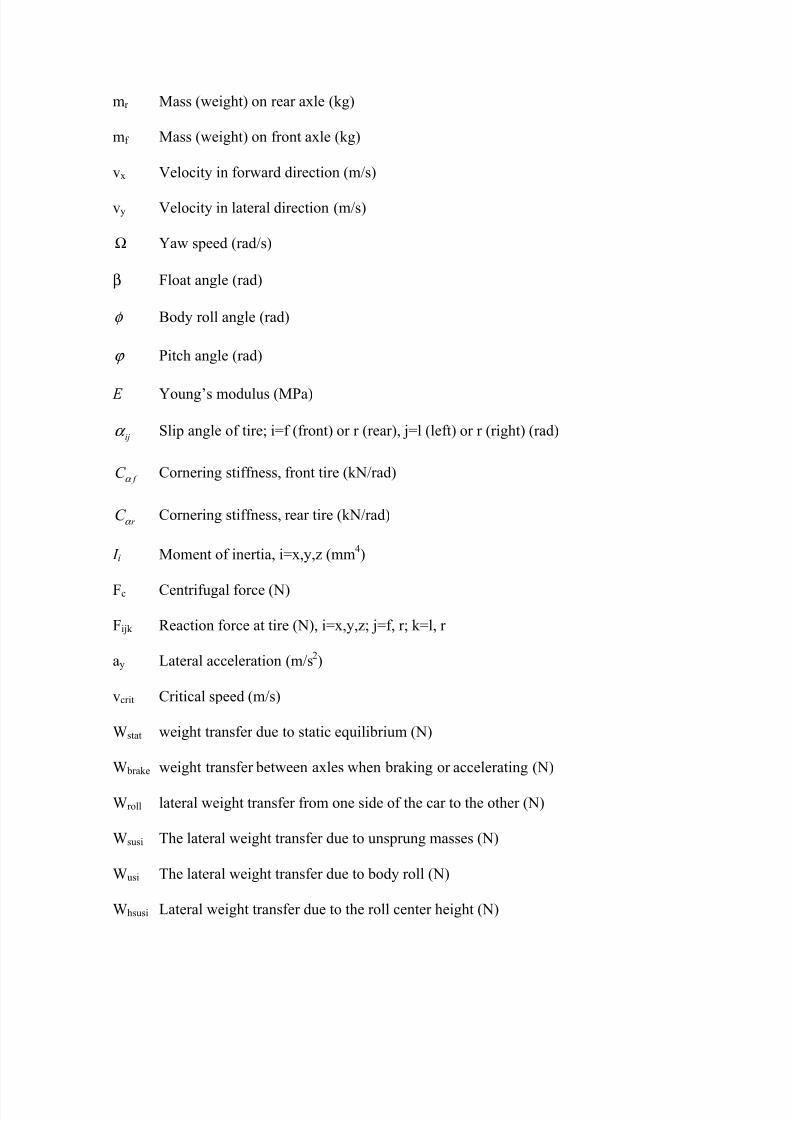
3.1 Slip angles

Thetiremodelpresentedneedstheslipangleα asinput.Theslipanglesaredefinedas

follows:

y

fl fl

x

y

rl rl

x

V +btan( - )=

V

V -ctan( - )=

V

f

r

t

t

δ α

δ α

⋅ Ω

+ ⋅ Ω

⋅ Ω

+ ⋅ Ω

(1.9)

y

fr fr

x

y

rr rr

x

V +btan( - )=

V

V -c

tan( - )= V

f

r

t

t

δ α

δ α

⋅ Ω

− ⋅ Ω

⋅ Ω

− ⋅ Ω

(1.10)

3.2 Vertical Loads

The normal reaction under each tire can be calculated using the Equation(1.11). It is

divided in three parts: Wstat which is a pure static equilibrium, W brake which is the amount of

weight transfer from one axle to another when braking or accelerating and Wroll which is the

lateral weight transfer from one side of the car to the other.

zi stat brake roll F W W W = + + (1.11)



2

2

2

2

zfl brake rollf

zfr brake rollf

zrl brake rollr

zrr brake rollr

mgc F W W

L

mgc F W W

L

mgb F W W L

mgc F W W

L

= + +

= + −

= + +

= + −

(1.12)

where

W brake

=

m susp

a xh

2 L+

musf a xhusf

2 L+

musr a xhusr

2 L(1.13)

and

rolli susi usi hsusiW W W W = + + (1.14)

i stands for either r or f and where Wsusi, Wusi and Whsusi are defined below.:

The lateral weight transfer due to unsprung masses is calculated as:

W usf = m

usf V y+V

xΩ( )

husf

2t f

W usr = m

usr V y+V

xΩ( )

husr

2t r

(1.15)

The lateral weight transfer due to body roll can be expressed as:

W susf

= m susp

V y+V

xΩ( )h1cosφ

K f

2t f

K ∑

W susr

= m susp

V y+V

xΩ( )h1cosφ

K r

2t r

K ∑

(1.16)

Lateral weight transfer due to the roll center height is expressed as:

W hsusf

= m susp

V y+V

xΩ( )

ch f

2 Lt f

W hsusr

= m susp

V y+V

xΩ( )

bhr

2 Lt r

(1.17)



3.3 Tire model

The elastic deformation of a tire is extremely complex due to the non-linearity and

theoretical computation requires numerical solution with for instance FEA. There are

several nonlinear tire models available, e.g. the CALSPAN tire model, the brush model or

the UMTRI model. However, industry and academia have reached apparent consensus in

recent years on the use of “magic formula”, developed by Pacejka et.al, [¡Error! No se

encuentra el origen de la referencia.] which summarizes experimental and theoretical data.

It allows one to compute forces at a higher precision than the common linearized

assumption, but without integrating equations. The tire model allows determination of all

six of the forces and moments generated by the tire: longitudinal force, lateral force,

vertical force, rolling resistance, overturning moment and self-aligning torque. Therefore,

forces can be computed in real-time. A pneumatic tire usually have a peak at about 4 to 6

degrees of slip where the cornering force decreases as slip increases on either side of the

peak. Past this peak, the vehicle will experience “dynamic understeer”, where turning the

wheel more makes the cornering conditions worse.

( )( )( )( ) sin arctan arctan y x C Bx E Bx Bx= − − (1.18)

( ) ( )v

h

Y X y x S

x X S

= +

= + (1.19)

The factor B is called the stiffness factor and it controls the slope of the curve at the origin.

The parameter C is called the shape factor and limits the range of the arguments in the sinus

function The parameter D is the maximum value the force or moment apart from the small



effect due to the S v term. The product BCD gives the slope and corresponds to the initial

cornering stiffness. S v and S h are the horizontal and vertical shift, respectively. They are

introduced to allow for non-zero forces and moments at zero slip. (See Wong [¡Error! No se

encuentra el origen de la referencia.] for details).

4 Control law

Many control laws can be implemented in order to minimize for instance the body roll or to

prevent over/under steer. There is a wealth of such control laws published in recent years

notable are the works of Abe [2] and Horiuchi [6]. The latter defines the control law as:

r r k k

δ δ δ

Ω= + Ω (1.20)

where

2 2( )

2

f

r

t y f r

r

r y

K k

K

mV bK cK k

K V

δ = −

+ −

=

(1.21)

This law is easy implemented in the model used. The equations presented in this article are

not in a closed form nor are they linearlized. That is not necessary because of the tools used

to resolve the equations. The model is done using MATLAB™/ SIMULINK™. Figure 2

shows the SIMULINK interface with all the equations represented. This chart is difficult to

assimilate therefore in Figure 3 a simplified chart is presented. It is a schematic and

simplified picture to show more clearly how the different parts are related.

An alternative algorithm is also evaluated. It is based upon the control scheme by Horiuchi

[6] but also monitors the forces on each wheel and if it is about to saturate then that



individual wheel changes the steering angle a certain amount so that the tires do not

saturate.

To do this a variable is introduces defined as:

zij

3

zij

F

2F1+

mg

zij B

µ =

⎛ ⎞ ⎜ ⎟

(1.22)

which is compared to the normal force of each tire, if the absolute value of this variable is

greater or equal to the normal force then no action is taken. On the contrary if the absolute

value of this variable is less than the normal force then the steering angle is changed

according to the equation (1.24) below. The steering angle, for the tire ij, is then changed

back to the original after two revolutions of the tire.

( ) ( 1) zij yij ij ij B F t t δ δ ≥ ⇒ = − (1.23)

3( ) ( 1)

5 zij yij ij ij

B F t t δ δ < ⇒ = − (1.24)

i=front or rear, j=left or right.

The novelty of this approach is that a single wheel can be steered independently of the rest

of the tires. For instance, if the vehicle travels in a curve to the right and accelerates at the

same time then weight will be transferred to the rear left. The lateral force, in an extreme

situation, may be close to saturating and thus staring to skid. Modifying that tire in such

away that the slip angle decreases would be a way to prevent the vehicle to skid and

consequently preventing it to become uncontrollable.

5 Results and Conclusion



The system varies the steer angle on the wheel with the highest loading between 0 and 1

degrees if the tire forces is about to saturate which depends on the road situation. If there is

a risk of skidding, the steer angle on one individual wheel is decreased by an appropriate

degree. It provides in the order of 10 to 25 percent more lateral stability than a conventional

system with 4WS. This significantly enhances active safety, since better lateral stability

equals superior road adhesion and better cornering stability.

An example simulation is made and the results are presented in Figure 4 to Figure 7. In

Figure 4 it can clearly be seen that the lateral acceleration decreases each time the control

systems modifies the steering angle. This can be on any single tire or on several it depend if

the condition (Equation (1.23) or (1.24) ) is satisfied or not. The effect is more notable in

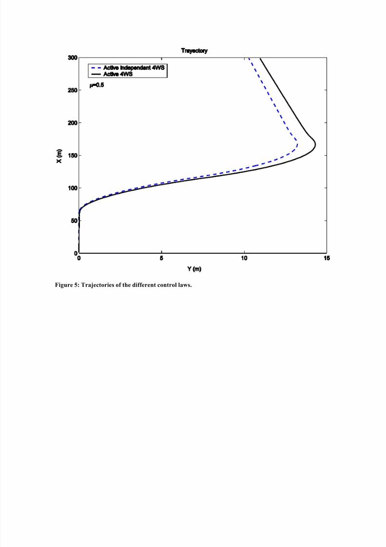
the lateral velocity which is noticeably diminished (Figure 6). This effect is also depicted in

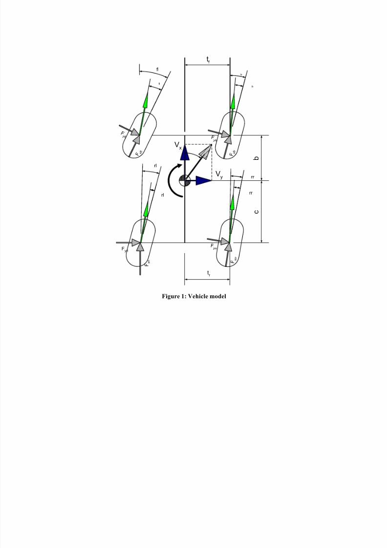
Figure 5. It is very interesting to plot the yaw rate versus the float angle (see β in Figure 1 )of the vehicle such as in Figure 7. Here it can be clearly seen that both the yaw velocity and

the float angle has improved. Particularly the float angle, which leads to more exact

handling and the ability to stay on track.



References

1. Ackermann, J. (1994) ‘Robust Decoupling, Ideal Steering Dynamics and Yaw

Stabilization of 4WS Cars’, Automatica, Vol.30, No.11.2. Abe, M. (1995) ‘Direct Yaw Moment Control for Improving Limit Performance of

Vehicle Handling - Comparison and Cooperation with 4WS’ 14th IAVSD

Symposium. 3. Sakai S., Sado H, and Hori Y., “Motion Control in an Electric Vehicle with 4

Independently Driven In-Wheel Motors” IEEE Trans. on Mechatronics, Vol. 4, No.1, pp.9-16, 1999.

4. Gibbs, J. and Chaplin, W. (1832) GB-patent 6241 from March 8th

.5. Nalecz, A.G. and Bindemann, A.C. (1989) ‘Handling Properties of Four Wheel

Steering Vehicles’ SAE Special Publications, No. 890080.6. Horiuchi, S. and Okada, K. (1999) ‘Improvement of a vehicle handling by nonlinear

integrated control of four wheel steering and four wheel torque’, JSAE Review Vol.20, pp. 459-464.



fr

rl rr

tf

tr

b

c

fl

fl

fr

F x f l

F y f l F

y f r

Fx

f r

Fyrl

F y r r

F x r l

Fx

r r

Vx

Vy rr

rl

Figure 1: Vehicle model



Figure 2: Simulink flowchart representing the 4WS dynamics simulation

Slipangles

Verticalloads

Steeringinput

Magic formulatire model

Vehicle model

dynamics

equations

Feedback to control system

Controlsystem

Output Figure 3: Data flow of the vehicle dynamics algorithm



Figure 4: Lateral acceleration vs. time



Figure 5: Trajectories of the different control laws.



Figure 6: Lateral velocity vs. time



Figure 7: Yaw velocity vs. slip angle β

Documents

Vehicle Dynamics With Independent 4WS