Embed Size (px)
Citation preview

International Journal of Theoretical Physics, Vol. 38, No. 7, 1999
Variance of the Quantum Coordinates of an Event
M. Toller1
Received November 18, 1998
We study the variances of the coordinates of an event considered as quantumobservables in a PoincareÂ-covariant theory. The starting point is their description interms of a covariant positive-operat or-valued measure on Minkowski space ±time.Besides the usual uncertainty relations, we find stronger inequalities involvingthe mass and the center-of-mass angular momentum of the object that definesthe event. We suggest that these inequalities may help to clarify some of thearguments which have been given in favor of a gravitational quantum limit tothe accuracy of time and space measurements.
1. INTRODUCTION
The word ª eventº is often used to indicate a point of the space±time
manifold. From the operational point of view this point has to be defined in
terms of some properties of a material object and the word ª eventº assumesa meaning which is not purely geometric, but is more similar to the meaning
it has in ordinary language, namely ª something that happensº in the physical
world. A typical event is the collision of two particles. Since the collision
of two small particles has a small probability, one may consider, more pre-
cisely, in the rest system of the center of mass (CM) the point which coincideswith the CM when the distance between the two particles reaches its minimum
value. This definition of an event makes sense in a classical (nonquantum)
theory in the absence of strong gravitational fields, which would complicate
the space±time geometry. In the example given above we have considered
a ª baricentric event,º which lies on the world line of the CM of the object
that defines it. There are also nonbaricentric events: for instance, a collisionof the first two particles in a system of three particles.
1 Department of Physics of the University and INFN I-38050 Trento, Italy; e-mail address:[email protected].
2015
0020-7748/99/0700-201 5$16.00/0 q 1999 Plenum Publishing Corporation

2016 Toller
If we take into account the quantum properties of the object that defines
an event, we have some difficult problems. The space±time coordinates x a
( a 5 0, 1, 2, 3) of the event with respect to a classical reference frame haveto be considered as quantum observables. The corresponding operators X a
have been defined and discussed by Jaekel and Reynaud (1996, 1997, 1998,
1999) in the framework of a conformally covariant quantum theory. A detailed
treatment of events in the framework of a PoincareÂ-covariant quantum theory
is given by Toller (1999) and the present article is a continuation of this
research, indicated by (I) in the following. Since, as shown by Pauli (1958)and Wightman (1962), the Hermitian operators X a cannot be self-adjoint, a
complete description of the coordinate observables has to be given in terms
of a positive-operator-valued measure (POVM) (Davies, 1976; Holevo, 1982;
Werner, 1986; Busch et al., 1991, 1995) defined on the Minkowski space±time
} and covariant with respect to the PoincareÂgroup. An explicit formula for
the most general PoincareÂ-covariant POVM is given in (I); it permits thecalculation of the operators X a . This treatment generalizes the analogous
treatment of the time observable discussed, for instance, by Busch et al.(1994), Giannitrapani (1997), and Muga et al. (1998).
Note that different measurement procedures are described by different
POVMs and there is in principle no reason to concentrate attention on oneof them. On the other hand, one cannot assume that every covariant POVM
describes a (possibly idealized) measurement procedure. The POVM formal-
ism is based on very general principles of relativity and quantum theory, but
other requirements may be relevant, for instance, superselection rules or
discrete symmetries such as time reversal. As a consequence, some care is
needed in the physical interpretation of our results.If the CM angular momentum does not vanish, the uncertainty relations
do not permit the definition an exactly baricentric event in a quantum theory,
but one can define an important class of POVMs, called quasibaricentric,
which describe events which happen as near as possible to the worldline of
the CM. From a POVM of this kind, assuming its covariance under dilatations,
one obtains exactly the operators X a defined and justified with good argumentsby Jaekel and Reynaud in the papers cited above. In Section 3 we characterize
the quasibaricentric POVMs by means of another physically relevant
condition.
If the state of the system is described by a normalized vector c P *,
the POVM t defines the probability that the event is detected in a set I ,}. Actually, one can write this probability in the form
( c , t (I ) c ) 5 # I
r ( c , x) d 4x (1)
where the density r ( c , x) is an integrable function. We have also shown in

Variance of the Quantum Coordinates of an Event 2017
(I) that the operators t (I ) have to vanish on the states with a singular four-
momentum spectrum, namely the vacuum and the one-particle states. There-
fore we consider a Hilbert space * that contains only states with a continuousmass spectrum, for instance, scattering states with two or more incoming
or outgoing particles. In the following we assume that t is normalized,
namely that
t (}) 5 1, # }
r ( c , x) d 4x 5 1, c P * (2)
This means that the event has to be found somewhere in space±time.The average value of a coordinate is given by
^ x a & 5 # x a r ( c , x) d 4x 5 ( c , X a c ) (3)
This equation defines the Hermitian coordinate operators X a , which in general
do not commute. Note, however, that the averages
^ (x a )2 & 5 # (x a )2 r ( c , x) d 4x (4)
in general cannot be written in the form
^ (x a )2 & 5 ( c , (X a )2 c ) 5 |X a c |2 (5)
and that the operators X a do not determine the POVM t univocally. There
are translation-covariant POVMs that satisfy Eq. (5), but this is not possible
if the PoincareÂcovariance is required. A general discussion of this problem(in a different context) is given by Werner (1986). It is important to remember
that the integrals (3) and (4) do not converge for all the choices of the vector
c and that the unbounded operators X a , like many other quantum observables,
are not defined on the whole Hilbert space *.
The purpose of the present article is to treat the quantities ^ (x a )2 & by
means of the formalism developed in (I). We can always choose a referenceframe in which ^ x a & 5 0 and in this frame ^ (x a )2 & is just the variance ( D x a )2.
It is also possible to choose the reference frame in such a way that the
positive-definite matrix ^ x a x b & is diagonal. In Section 2 we show that the
indeterminacy relations
D x a D k a $1
2, c 5 " 5 1 (6)
where k is the four-momentum of the system that defines the event, are valid
in general, even if the proof is more complicated than the usual one.
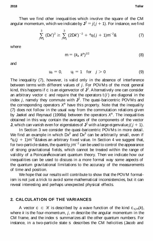
2018 Toller
Then we find other inequalities which involve the square of the CM
angular momentum, which we indicate by J2 5 j( j 1 1). For instance, we find
o3
r 5 1
( D xr)2 $ o3
r 5 1
(2 D kr) 2 2 1 ^ u j( j 1 1) m 2 2 & (7)
where
m 5 (k a k a )1/2 (8)
and
u 0 5 0, u j 5 1 for j . 0 (9)
The inequality (7), however, is valid only in the absence of interference
between terms with different values of j. For POVMs of the most general
kind, this happens if c is an eigenvector of J2. Alternatively one can consider
an arbitrary vector c and require that the operators t (I ) are diagonal in the
index j, namely they commute with J2. The quasi-baricentric POVMs and
the corresponding operators X a have this property. Note that the inequality(7) does not follow in the usual way from the commutation relations given
by Jaekel and Reynaud (1998a) between the operators X a . The inequalities
obtained in this way contain the averages of the components of the vector
J, which can vanish even for eigenstates of J2 with a large eigenvalue j( j 1 1).
In Section 3 we consider the quasi-baricentric POVMs in more detail.
We find an example in which D x0 and D x3 can be arbitrarily small, even if^ u j (j 1 1) m 2 2 & takes an arbitrary fixed value. In Section 4 we suggest that,
for two-particle states, the quantity j m 2 2 can be used to control the appearance
of strong gravitational fields, which cannot be treated within the range of
validity of a PoincareÂ-covariant quantum theory. Then we indicate how our
inequalities can be used to discuss in a more formal way some aspects of
the quantum gravitational limitations to the accuracy of the measurementsof time and position.
We hope that our results will contribute to show that the POVM formal-
ism is not just a trick to avoid some mathematical inconsistencies, but it can
reveal interesting and perhaps unexpected physical effects.
2. CALCULATION OF THE VARIANCES
A vector c P * is described by a wave function of the kind c s jm(k),
where k is the four-momentum, j, m describe the angular momentum in the
CM frame, and the index s summarizes all the other quantum numbers. For
instance, in a two-particle state s describes the CM helicities (Jacob and

Variance of the Quantum Coordinates of an Event 2019
Wick, 1959). Since c has a continuous four-momentum spectrum, its norm
can be written in the form
| c |2 5 # Vos jm
) c s jm (k) ) 2 d 4k (10)
where V is the open future cone. Note that j and the mass m label the
equivalence classes of irreducible unitary representations of the PoincareÂ
group, which act on the wave functions c s jm(k) in the way described byWigner (1939).
We showed in (I) that the probability density is given by
r ( c , x) 5 # Goln
) C g ln(x) ) 2 d v ( g ) (11)
where
C g ln(x) 5 (2 p ) 2 2 # V
exp( 2 ix a k a ) ojm
DMclnjm (ak) f g jm(k) d 4k (12)
We have introduced the new function
f g jm(k) 5 os
F jg s ( m ) c s jm(k) (13)
The quantities F jg s ( m ) are complex functions of m which characterize the
particular POVM. The quantities DMcjmj8m8(a) are the matrix elements of the
irreducible unitary representations of SL(2, C ) described by Naimark (1964),Gel’ fand et al. (1966), and RuÈ hl (1970). The possible values of the indices are
M 5 0, 61
2, 6 1, . . . , c2 , 1
j 5 ) M ) , ) M ) 1 1, . . . , m 5 2 j, 2 j 1 1, . . . , j (14)
If M Þ 0, c must be imaginary. The representations DMc and D 2 M , 2 c are
unitarily equivalent. According to our conventions, D01 is the trivial one-dimensional representation with only one matrix element given by
D010000(a) 5 1 (15)
The variable g P G stands for a discrete index n and the parameters M, cwhich label the irreducible unitary representations of SL(2, C ); v is a positive
measure on the space G . For the Wigner boost we use
ak 5 (2 m ( m 1 k0)) 2 1/2 ( m 1 k0 1 ks s s) P SL(2, C ) (16)
where s s are the Pauli matrices. Here and in the following the indices a , b

2020 Toller
take the values 0, 1, 2, 3 and the indices r, s, t, u, v take the values 1, 2, 3. The
summation convention is applied to both kinds of indices. The normalization
condition (2) gives rise to the constraint
# G
F jg s ( m ) F j
g s 8( m ) d v ( g ) 5 d s s 8 (17)
and to the equation
# G # Vojm
) f g jm(k) ) 2 d 4k d v ( g ) 5 | c |2 (18)
In order to compute the averages (3) and (4), we note that we have, in
the sense of distribution theory,
x a C g ln(x) 5 2 i(2 p ) 2 2 # V
exp( 2 ix a k a )
3 ojm
-- k a (DMc
lnjm(ak) f g jm (k)) d 4k (19)
In this way we obtain, if c is chosen in such a way that the integral is
meaningful and convergent,
^ (x a )2 & 5 # G # Vojm
) [Y a f ] g jm(k) ) 2 d 4k d v ( g ) (20)
where the operators Y a are defined by
[Y a f ] g jm(k) 5 oj8m8
SMca jmj8m8 (k) f g j8m8(k) 2 i
-- k a f g jm(k) (21)
and we have introduced the Hermitian matrices
SMca jmj8m8(k) 5 2 i o
lnDMc
jmln(a 2 1k )
-- k a DMc
lnj8m8(ak) (22)
These matrices, as we showed in (I), are given by
SMc0jmj8m8(k) 5
1
m 2 kr N rMcjmj8m8 (23)
SMcrjmj8m8(k) 5 2
1
mN rMc
jmj8m8
21
m 2( m 1 k0)krksN sMc
jmj8m8 11
m ( m 1 k0)d jj8 e
rstksM tjmm8 (24)
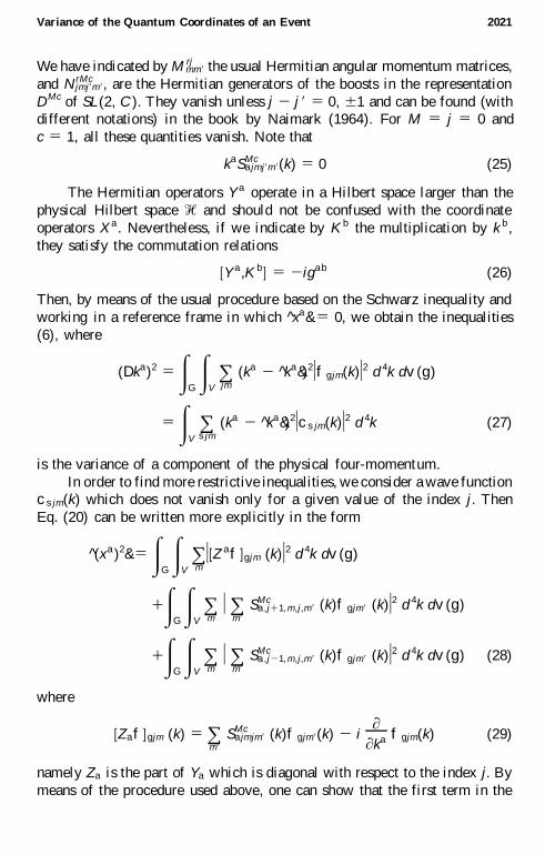
Variance of the Quantum Coordinates of an Event 2021
We have indicated by M rjmm8 the usual Hermitian angular momentum matrices,
and N rMcjmj8m8, are the Hermitian generators of the boosts in the representation
DMc of SL(2, C ). They vanish unless j 2 j 8 5 0, 6 1 and can be found (withdifferent notations) in the book by Naimark (1964). For M 5 j 5 0 and
c 5 1, all these quantities vanish. Note that
k a SMca jmj8m8(k) 5 0 (25)
The Hermitian operators Y a operate in a Hilbert space larger than the
physical Hilbert space * and should not be confused with the coordinate
operators X a . Nevertheless, if we indicate by K b the multiplication by k b ,
they satisfy the commutation relations
[Y a ,K b ] 5 2 ig a b (26)
Then, by means of the usual procedure based on the Schwarz inequality and
working in a reference frame in which ^ x a & 5 0, we obtain the inequalities
(6), where
( D k a )2 5 # G # Vojm
(k a 2 ^ k a & )2 ) f g jm(k) ) 2 d 4k d v ( g )
5 # Vos jm
(k a 2 ^ k a & )2 ) c s jm(k) ) 2 d 4k (27)
is the variance of a component of the physical four-momentum.
In order to find more restrictive inequalities, we consider a wave functionc s jm(k) which does not vanish only for a given value of the index j. Then
Eq. (20) can be written more explicitly in the form
^ (x a )2 & 5 # G # Vom
) [Z a f ] g jm (k) ) 2 d 4k d v ( g )
1 # G # Vom
) om8
SMca , j 1 1,m, j,m8 (k) f g jm8 (k) ) 2 d 4k d v ( g )
1 # G # Vom
) om8
SMca , j 2 1,m, j,m8 (k) f g jm8 (k) ) 2 d 4k d v ( g ) (28)
where
[Z a f ] g jm (k) 5 om8
SMca jmjm8 (k) f g jm8(k) 2 i
-- k a f g jm(k) (29)
namely Z a is the part of Y a which is diagonal with respect to the index j. By
means of the procedure used above, one can show that the first term in the

2022 Toller
right-hand side has the lower bound (2 D k a ) 2 2 and the other two terms, which
do not contain derivatives, improve this lower bound.
From the results given by Naimark (1964) we obtain, in agreement withthe Wigner±Eckart theorem, the following useful formulas:
N rMcjmjm8 5
2 iMc
j( j 1 1)M rj
mm8 (30)
om9
N rMcj,m, j 1 1,m9 N sMc
j 1 1,m9, j,m8
5 QMcj 1 1 1 ( j 1 1)2 d rs d mm8 2 o
m9M rj
mm9Msjm9m8 2 i( j 1 1) e rstM tj
mm8 2 (31)
om9
N rMcj,m, j 2 1,m9 N sMc
j 2 1,m9, j,m8
5 QMcj 1 j2 d rs d mm8 2 o
m9M rj
mm9Msjm9m8 1 ij e rstM tj
mm8 2 (32)
where
QMcj 5
( j2 2 M 2)( j2 2 c2)
j2(2j 1 1)(2j 2 1), j $ 1 (33)
From these formulas we obtain
om9
SMc0, j,m, j 1 1,m9 SMc
0, j 1 1,m9, j,m8 5 m 2 4 QMcj 1 1 A j
mm8(k) (34)
om9
SMcr, j,m, j 1 1,m9 SMc
r, j 1 1,m9, j,m8 (35)
5 m 2 2QMcj 1 1 ( j 1 1)(2j 1 3) d mm8 1 m 2 4QMc
j 1 1Ajmm8(k)
where
Ajmm8(k) 5 krkr( j 1 1)2 d mm8 2 krks o
m9M rj
mm9Msjm9m8 (36)
is a positive-definite matrix.
Then, in a reference frame in which ^ x a & 5 0, by means of the inequality
QMcj 1 1 $ u j (2j 1 3) 2 1, ) M ) # j (37)
we obtain the inequalitiy (7). We have to remember that it has been proven
under the assumption that c is an eigenvector of J2. Its general validity can
be excluded: we have just to consider a nonbaricentric POVM which describes
a collision of the first two particles in a system of three particles. Then,
Variance of the Quantum Coordinates of an Event 2023
if the third particle is sufficiently distant, the total center-of-mass angular
momentum j can be made as large as we want without increasing the CM
energy m and without affecting the variance of the coordinates of the consid-ered event.
3. QUASI-BARICENTRIC EVENTS
In order to minimize the second term in Eq. (28), we have to require
that the equality sign holds in Eq. (37), namely that
F jn Mc s ( m ) Þ 0 only if
M 5 j, c 5 1 for j 5 0 and c 5 0 for j . 0. (38)
Under the same conditions, the third term in Eq. (28) vanishes. This is
the definition of quasi-baricentric POVM introduced in (I) with a different
motivation. We may say that the quasi-baricentric POVMs minimize the
variances of the coordinates when c is an eigenvector of J2.If the condition (38) is valid, the index j is uniquely fixed by the index
g 5 { n , M, c} and no interference term can appear. Then we expect that the
inequality (7) derived in the preceding section is valid for a quasi-baricentric
measure without any limitation of the wave function c . In order to study this
inequality in more detail, we rewrite the formulas given in the preceding
section in a simpler form; in particular, we replace the integration over thevariable g 5 { n , M, c} by a sum over the indices n and M 5 j. In this way
we obtain
r ( c , x) 5 on jln
) C n jln(x) ) 2 (39)
C n jln(x) 5 (2 p ) 2 2 # V
exp( 2 ix a k a ) om
D jclnjm(ak) f n jm(k) d 4k (40)
f n jm(k) 5 os
F jn s ( m ) c s jm(k) (41)
where the quantities
F jn s ( m ) 5 F j
n jc s ( m ) (42)
have the normalization property
on
F jn s ( m ) F j
n s 8 ( m ) 5 d s s 8 (43)
In all these formulas, the parameter c takes the values given in Eq. (38).

2024 Toller
Equation (20) can be written in the form
^ (x a )2 & 5 |Z a f |2 1 # Von jm Z o
m8S jc
a , j 1 1,m, j,m8 (k) f n jm8(k) Z2
d 4k (44)
where
|Z a f |2 5 # Von jm
) [Z a f ] n jm (k) ) 2 d 4k (45)
For a quasi-baricentric measure the operators Z a defined by Eq. (29) takethe form
Z0 5 2 i-
- k0 (46)
Zr 5 m 2 1( m 1 k0) 2 1 e rstksM tj 2 i-
- kr (47)
where M tj are the angular momentum matrices which act on the index m of
f n jm(k). These operators satisfy the commutation relations
[Z a , K b ] 5 2 i d ba (48)
[Z0, Zr] 5 i m 2 3 e rstksM tj (49)
[Zr , Zs] 5 i m 2 3(k0 e rsu 2 ( m 1 k0) 2 1 e rsvkvku)M uj (50)
These relations permit us, in the usual way, to obtain inequalities for the
quantities i Z a f |. In particular, using also Eq. (35), one can derive the inequal-
ity (7).
It is interesting to consider the case in which
F jn s ( m ) 5 d n s , f n jm(k) 5 c n jm(k) (51)
Then the operators Z a operate in the physical Hilbert space * and they are
just the coordinate operators X a . From Eq. (44) we see that Eq. (5) cannotbe true, but there are additional contributions to the variance.
In order to obtain a better understanding of Eq. (44), we examine a
simple model. We consider a quasi-baricentric POVM which satisfies Eq.
(51); we assume that the index s 5 n can take only one value and we drop
it in the following formulas. Then we consider a particular sequence ofvectors c (j) given by
c (j)j8m(k) 5 d j8j d mj f(q)j 2 3/8 (52)

Variance of the Quantum Coordinates of an Event 2025
where
q0 5 j 2 1/2 k0, q1 5 k1, q2 5 k2, q3 5 j 2 1/4k3 (53)
and we compute the limit of the variances for j ® ` . In this limit the CM
angular momentum becomes very large and is directed along the x3 axis; the
variances of k0 and k3 tend to infinity in a different way and the componentskr(k0) 2 1 of the CM velocity become very small. By means of a change of
variables, we see that the normalization condition of the vectors c (j) is given by
| c (j)|2 5 # ) f(q) ) 2 d 4q 5 1 (54)
and that we have the finite limit
limj ® `
^ ( j 1 1) m 2 2 & 5 # ) f(q) ) 2(q0) 2 2 d 4q 5 A (55)
By means of the formulas given in the preceding section and of the
known form of the angular momentum matrices matrices Mrj, we obtain after
some calculations
limj ® `
^ (x0)2 & 5 limj ® `
^ (x3)2 & 5 0 (56)
limj ® `
^ (x1)2 & 5 # ) 12
q2 (q0) 2 2 f(q) 2 i-
- q1 f(q) ) 2 d 4q 11
2A (57)
limj ® `
^ (x2)2 & 5 # ) 21
2q1(q0) 2 2 f(q) 2 i
-- q2 f(q) ) 2 d 4q 1
1
2A (58)
We see that if we fix the quantity ^ ( j 1 1) m 2 2 & , the quantities D x0 and D x3
can be arbitrarily small. The integrals in the last two formulas cannot be
neglected with respect to A, as follows from the commutation relations (50).
We can show that they can be made of the order of A by computing them
for a special choice of f(q), namely
f(q) 5 (2 p ) 2 1/2 (q0) 2 1 exp { 2 (2q0) 2 2[(q1)2 1 (q2)2]} g(q0, q3) (59)
The result is
limj ® `
^ (x1)2 & 5 limj ® `
^ (x2)2 & 5 A (60)
4. PERIPHERAL COLLISIONS
Many arguments indicate that the quantum gravitational effects give rise
to some limitations to the precision of time and position measurements; a
2026 Toller
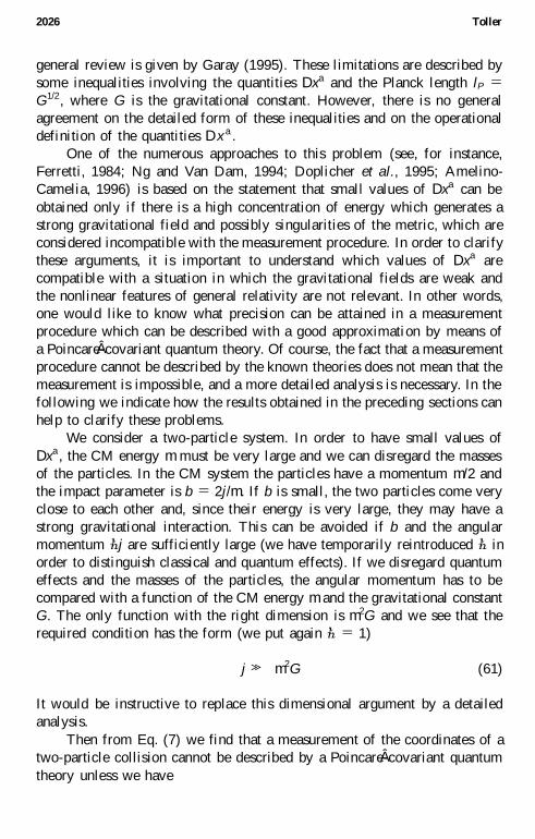
general review is given by Garay (1995). These limitations are described by
some inequalities involving the quantities D x a and the Planck length lP 5G1/2, where G is the gravitational constant. However, there is no general
agreement on the detailed form of these inequalities and on the operational
definition of the quantities D x a .
One of the numerous approaches to this problem (see, for instance,
Ferretti, 1984; Ng and Van Dam, 1994; Doplicher et al., 1995; Amelino-
Camelia, 1996) is based on the statement that small values of D x a can be
obtained only if there is a high concentration of energy which generates a
strong gravitational field and possibly singularities of the metric, which are
considered incompatible with the measurement procedure. In order to clarify
these arguments, it is important to understand which values of D x a are
compatible with a situation in which the gravitational fields are weak and
the nonlinear features of general relativity are not relevant. In other words,
one would like to know what precision can be attained in a measurement
procedure which can be described with a good approximation by means of
a PoincareÂ-covariant quantum theory. Of course, the fact that a measurement
procedure cannot be described by the known theories does not mean that the
measurement is impossible, and a more detailed analysis is necessary. In the
following we indicate how the results obtained in the preceding sections can
help to clarify these problems.
We consider a two-particle system. In order to have small values of
D x a , the CM energy m must be very large and we can disregard the masses
of the particles. In the CM system the particles have a momentum m /2 and
the impact parameter is b 5 2j/ m . If b is small, the two particles come very
close to each other and, since their energy is very large, they may have a
strong gravitational interaction. This can be avoided if b and the angular
momentum " j are sufficiently large (we have temporarily reintroduced " in
order to distinguish classical and quantum effects). If we disregard quantum
effects and the masses of the particles, the angular momentum has to be
compared with a function of the CM energy m and the gravitational constant
G. The only function with the right dimension is m 2G and we see that the
required condition has the form (we put again " 5 1)
j À m 2G (61)
It would be instructive to replace this dimensional argument by a detailed
analysis.
Then from Eq. (7) we find that a measurement of the coordinates of a
two-particle collision cannot be described by a PoincareÂ-covariant quantum
theory unless we have

Variance of the Quantum Coordinates of an Event 2027
o3
r 5 1
( D x r )2 À G 5 l 2P (62)
We have already remarked that this does not mean that a more precise
measurement is impossible.
It also follows from the results of Section 3 that the condition (61) does
not imply any restriction on the quantities D x0 and, for instance, D x3. In this
case, too, we have to be careful, because it is not sure that the POVMs
that permit arbitrarily small values of D x0 and D x3 correspond to physicalmeasurement procedures. In other words, we could have disregarded some
relevant physical condition. Moreover, the space±time uncertainty relations
can also be introduced by means of arguments which are not based on the
unwanted appearance of strong gravitational fields (see, for instance, Mead,
1964; Jaekel and Reynaud, 1994).
We shall discuss these problems in more detail elsewhere. Here our aimis just to suggest that the inequality (7) may play a role in the discussion of
the space±time uncertainty relations due to quantum gravity.
REFERENCES
Amelino-Camel ia, G. (1996). Modern Physics Letters A, 11, 1411.
Busch, P., Lahti, P. J., and Mittelstaedt, P. (1991). The Quantum Theory of Measurement ,
Springer-Verlag, Berlin.
Busch, P., Grabowski, M., and Lahti, P. J. (1994). Physics Letters A, 191 , 357.
Busch, P., Grabowski, M., and Lahti, P. J. (1995). Operational Quantum Physics, Springer
Verlag, New York.
Davies, E. B. (1976). Quantum Theory of Open Systems, Academic Press, London.
Doplicher, S., Fredenhagen, K., and Roberts, J. E. (1995). Communications of Mathematical
Physics, 172 , 187.
Ferretti, B. (1984). Lettere al Nuovo Cimento, 40, 169.
Garay, L. J. (1995). International Journal of Modern Physics A, 10, 145.
Gel’ fand, I. M., Graev, M. I., and Vilenkin, N. Ya. (1966). Generalized Functions, Vol. 5,
Academic Press, New York.
Giannitrapani, R. (1997). International Journal of Theoretical Physics, 36, 1575.
Holevo, A. S. (1982). Probabilistic and Statistical Aspect of Quantum Theory, North-Hol-
land, Amsterdam.
Jacob, M., and Wick, G. C. (1959). Annals of Physics, 7, 404.
Jaekel, M. T., and Reynaud, S. (1994). Physics Letters A, 185 , 143.
Jaekel, M. T., and Reynaud, S. (1996). Physics Letters A, 220 , 10.
Jaekel, M. T., and Reynaud, S. (1997). Europhysics Letters 38, 1.
Jaekel, M. T., and Reynaud, S. (1998). Foundations of Physics, 28, 439.
Jaekel, M. T., and Reynaud, S. (1999). European Physical Journal D5, 9.
Mead, C. A. (1964). Physical Review, 135B , 849.
Muga, J. G., Leavens, C. R., and Palao J. P. (1998). Physical Review A, 58, 9336.
Naimark, M. A. (1964). Linear Representations of the Lorentz Group . Pergamon Press, London.

2028 Toller
Ng, Y. J., and Van Dam, H. (1994). Modern Physics Letters A, 9, 335.
Pauli, W. (1958). Die allgemeinen Prinzipien der Wellenmechanik , Handbuch der Physik, Vol.
V/1, S. FluÈ gge, ed. Springer-Verlag, Berlin, p. 60.
RuÈ hl, W. (1970). The Lorentz Group and Harmonic Analysis, Benjamin, New York.
Toller, M. (1999). Physical Review A, 59, 960.
Werner, R. (1986). Journal of Mathematical Physics, 27, 793.
Wightman, A. S. (1962). Reviews of Modern Physics, 34, 845.
Wigner, E. P. (1939). Annals of Mathematics , 40, 149.


![Interpolation via Barycentric Coordinates · • Moving least squares coordinates [Manson and Schaefer, 2010] • Cubic mean value coordinates [Li and Hu, 2013] • Poisson coordinates](https://img.pdfslide.us/doc/110x75/6062738927364e51e610e629/interpolation-via-barycentric-coordinates-a-moving-least-squares-coordinates-manson.jpg)


![arXiv:0704.0796v4 [quant-ph] 16 Jul 2007The associated variance is then a measure of quantum fluctuations associated with the environment state, and is the source of quantum “noise”](https://img.pdfslide.us/doc/110x75/60063a61139161124e0ad481/arxiv07040796v4-quant-ph-16-jul-2007-the-associated-variance-is-then-a-measure.jpg)