Variance Forecast Performance Measures:

An Economic Approach ∗

Natalia Sizova†

Duke University

First Version: February 6, 2008

Current Version: November 2, 2008‡

Abstract

This paper introduces an economically motivated performance measure for variance forecasts

based on variance trading. The performance measure is constructed within a microeconomic

framework that mimics the decision-making process of a variance trader who uses volatility

forecasts to predict future profitability of a trade. The new performance measure can serve as

a useful complement to more traditional statistical criteria, by focusing on the economic value

contained in variance forecasts.

1 Introduction

Statistical forecast performance measures such as mean-squared error (MSE), mean-absolute error

(MAE), median-absolute error, and similar statistics are sometimes found to be unsatisfactory from

an economic point of view. For instance, Leith and Tanner (1991) found that MSE and MAE are un-

correlated with profit-losses derived from forecasting of interest rates. Figlewski and Thomas(1983)

found inconsistencies between statistical measures and profits for evaluation of money supply fore-

casts. West, Edison, and Cho (1993), and also Eun and Resnick (1984) give further evidence that

the MSE-criterion is not the best measure of forecast performance.

Statistical criteria also exhibit certain features, such as symmetry, that do not pertain to the

forecasts reported by forecasting agencies. For example, Patton and Timmermann (2007) found∗I would like to thank my advisor Tim Bollerslev, and committee members, George Tauchen, Bjørn Eraker, and

Shakeeb Khan, for their useful suggestions. I also thank participants of the Duke Econometrics and Finance Lunch

Group and participants of the UNC Kenan-Flagler Brown Bag Seminars for their helpful comments. All remaining

errors are my own.†Department of Economics, Duke University Box 90097, Durham, NC 27708. Phone: (713)775-5365. email:

natalia.sizova@duke.edu.‡Preliminary Version. Comments are Welcome!

1

that the economy growth forecasts reported by the Federal Reserve Board are downward biased,

i.e. the FRB employs an asymmetric criterion.

As alternative to the statistical criteria, forecast performance can be measured by utility-based

loss-functions, which naturally follow from applications of forecasts and are consistent with internal

preferences of forecasters. For example, the loss-function based on utility of the portfolio manager

who uses variance forecasts for mean-variance optimization is suitable to measure the accuracy

of variance-covariance matrices; see Kirby, Flemming, and Ostdiek(2001, 2003), West, Edison,

and Cho (1993). Another utility-based approach is designed to measure the accuracy of forecasts

for asset prices. It is based on profits that are derived from trading these assets; see Leith and

Tanner(1991), Guo (2006), Johannes, Stroud and Polson (2003), and Johannes, Korteweg, and

Polson (2008). Under this type of “profit” loss-function, the success of a forecast depends not only

on the forecast and the actual value, but also on a third variable – market price. From no-arbitrage

considerations a market price represents a forecast itself. Therefore, “profit” loss-functions favor

forecasts that can outperform this “aggregate” forecast, i.e. that can correctly identify mispricing

in the market. However, statistical measures of forecast performance do not account for this third

variable. They consider the forecast and actual value in isolation from other external factors.

We extend the latter type of utility-based performance measure to the case of univariate volatil-

ity forecasting. We develop a performance measure that tracks the mispricing of the variance in

the market. To define the market price for the variance, we need to find securities that enable

betting on volatility, e.g. call and put options. Future volatility plays so important a role in option

trading defining the price and volumes of option markets, that the phrase “to buy and sell volatil-

ity” has become a standard way to refer to buying and selling options. The information about

variance that is entering option prices can be synthesized to create a pure tool to bet on volatility

– variance swap. It can be expected that sensible forecast methods should benefit variance swap

trading strategies. Thus, a loss-function based on the utility of a variance swap trader who employs

a particular forecast can be a valid measure of forecast comparison.

In this study we compare two broad groups of forecasts of variance that we will refer to

as model-based and reduced-form respectively. The first group includes generally sophisticated

methods that form “ efficient” variance forecasts based on fully specified models for returns, e.g.

ARCH and SV models as reviewed by Andersen, Bollerslev, Christoffersen and Diebold (2005)

and Tauchen(2004). Forecasts in the second group are based on linear regressions for observable

variance proxies, such as HAR models by Corsi(2004) and ARFIMA models by Andersen, Boller-

slev, Diebold and Labys(2003). Despite their simplicity, the forecasts in the latter group perform

very often on par and sometimes better than the best forecasts in the first group; see Andersen,

Bollerslev, and Meddahi (2004), Sizova(2008). Our goal is to determine if the same finding holds

for utility-based performance measures.

We show that the forecasts from both groups provide economic value for risk-averse traders. In

2

terms of compensations, the advantage from using a forecast is worth a fee up to 5% - 10% of the

contract price relative to the maximum utility from the strategies that do not rely on forecasts.

We demonstrate that to be able to compete with reduced-form forecasts, a model-based forecast

has to employ high-frequency data and exhibit a sufficiently rich structure. Such a forecast and a

simple linear reduced-form forecast are close in performance, the first being marginally better for

low-uncertainty periods and the latter being slightly better for high-uncertainty periods. In terms

of compensations, less risk-averse traders are willing to pay no more than 1 % of the contract price

to switch from a model-based forecast to a reduced-form forecast, and more risk-averse traders are

willing to pay no more than 0.5% of the contract price to make the opposite switch.

The paper is organized as follows. Section 2 defines the variance swap. In Section 3, we

propose a model of a variance swap trader. In Section 4, we define loss functions based on variance

swap trading. In Section 5, we introduce the forecasts to be compared and describe estimation

methodologies. In Section 6, we compare those forecasts for the observed data on S&P 500 futures

and VIX data. Section 7 replicates the comparison using simulated data, and section 8 summarizes

the main findings.

2 Variance Swap as a Benchmark for Forecasts

The loss function to be introduced in this paper compares the ability of variance forecasts to predict

that the variance will be larger or lower than the level implied by derivative prices. For example,

this level can be set by prices of variance swaps, the derivatives that summarize the variance

information contained in options. Variance swap is a forward contract that allows to hedge against

future volatility. It has two “legs”. One “leg” of the swap will pay the realized variance over a

specified period [t, t + H], say RV t+Ht . The other “leg” of the swap will pay a fixed amount, the

strike price Pt. All the cash flows are exchanged on the maturity of the contract at t + H. At this

time the buyer of the swap receives the difference Ct+H = RV t+Ht − Pt. Therefore, if initially the

buyer was exposed to the volatility in the underlying security, then after buying such a contract he

reduces his exposure. His losses are bounded by the price Pt, since RV t+Ht is positive.

The value for the realized variance is defined in the following way. Suppose that the log-price

of the underlying security st (e.g. stock index) is observed at discrete times t, t+h, t+2h, ..., t+H.

Then, the realized variance over the period [t, t + H] is defined as the sum of squared returns:

RV t+Ht =

H/h∑

j=1

(st+jh − st+jh−h)2 . (1)

The realized variance, as defined above, is a proxy for the integrated variance that is a measure

of the return variability; see Andersen and Bollerslev(1998), and Barndorff-Nielsen and Shephard

(2002). Therefore, the realized variance (RV) itself is a valid measure of the financial volatility, and

3

the variance swaps are pure tools to bet on the volatility. For instance, if one expects variance to

soar, he may buy a variance swap to profit from this expectation. 1

In the variance swap contract there are two participating counterparts: variance seller and

variance buyer. In the following, we will assume that variance buyer is a large investor with a

diversified portfolio who for a given price Pt has a fixed demand K for variance swaps. In contrast,

variance seller is a trader who does not hold a diversified portfolio. In the next section we build

a model for a variance swap seller who facing the order of size K evaluates the chances that

the realized variance will be sufficiently lower than the price Pt, thus giving him a premium for

undertaking the risk.

3 Model of a Variance Seller

The variance seller caters to large clients who are willing to hedge their investment portfolios against

rough movements of the stock market by buying inelastically K variance swap contracts with a

maturity H. Therefore, the seller shorts variance and his profit-losses are equal to K(Pt(H) −RV t+H

t ), where Pt(H) is the price of the contract. For providing a sell-side for this transaction,

the trader certainly requires a premium, since he takes on the risk of unbounded losses. The seller

can refrain from trading if he thinks that the offered premium is not high enough to compensate

for the risk associated with the trade.

The minimum price that is required by the trader depends on his own forecast of the future

variance. Overestimation of the future variance results in lost trading opportunities, and underesti-

mation results in losses. Therefore, a more accurate forecast enables a more accurate decision rule

for wether trade or not to trade. Consequently, for each forecast there is a corresponding utility of

a trader who uses this forecast to form his trading strategy.

In this section, we build a model of a variance seller with a given utility over his cash flows.

Based on this model, a loss-function will be defined. The model will be presented in the following

steps. First, we will define the trader’s cash flows. Second, we will find the optimal trading rule for

an arbitrary utility. Third, we will specify the family of utility functions. Finally, we will specify

the exogenous market price of the variance swap.

Let us start by defining the trader’s cash flows. If the trader agrees to sell the variance at the

price Pt(H), then after H periods, he will receive the difference between this price and the realized

variance K(Pt(H) − RV t+Ht ). If he refuses to participate in this contract, he will be idle for this

period and his cash flows from variance swap selling on the date t + H will be zero. Therefore, his1Variance betting is not the only reason for trading variance swaps. Besides speculation, they can be used to hedge

against strong downward movements in the market. This hedge is possible due to the robust correlation between

directional and volatility risks; see Bollerslev, Zhou, and Tauchen(2008), and Drechsler and Yaron(2008) for a general

equilibrium explanation of this phenomenon.

4

action space is an indicator of an undertaken trade It ∈ 0, 1. The corresponding cash flows at

time t + H are equal to

Ct+H =[Pt(H)−RV t+H

t

]KIt. (2)

Cash flows of the trader are positive for low realized variance and negative for high realized variance.

This variability induces a risk of large losses. Therefore, in general a trader will require a risk

premium to trade, i.e. the trader will sell the contract only if the price Pt(H) is high enough to

remunerate the trader for the risk. We can give analytical content to this statement if we specify

the utility of the trader over his cash-flows.

Suppose, the trader is myopic and his objective function is given by the risk-adjustment operator

Vt(Ct+H). For a given objective, the optimal decision of the trader to trade or not to trade is defined

through the optimization:

I∗t = arg maxIt∈0,1

Vt(Ct+H)

s.t. Ct+H =[Pt(H)−RV t+H

t

]KIt.

(3)

We assume the strict monotonicity of the operator Vt(.). If Vt(.) is strictly increasing, then there

exists a reservation value Pt(H) such that the trader trades if and only if Pt(H) > Pt(H), i.e.

I∗t = I(Pt(H) > Pt(H)), (4)

and this value can be found from the rationality constraint:

Vt(0) = Vt(K[Rt(H)−RV t+Ht ]). (5)

Hence, in this model, a trader will not swap the variance if and only if his internal valuation of the

variance is higher than the one implied by the market’s Pt. This can happen for the following three

reasons. First, his risk-aversion can be higher than the current risk aversion of the market partici-

pants on average (the “aggregate investor”). Second, the inelastic transaction size K(notional) can

be higher than typically traded on the market, making the trader more cautious about undertaking

the risk. Third, he may employ a forecasting method that gives him an advantage in comparison

to the forecasting methods used by the market participants, which allows him to avoid unprofitable

trades.

3.1 Utility Specification

Prior to specifying the class of utilities, we will define the properties that are required from this class

given the objectives of this paper. First, our focus is only on the prediction of the realized variance

level. Because most of the literature deals with the prediction of RV, we believe considering only

5

the RV forecasts is the most relevant first step. 2 Considering that our focus in on the prediction

of the realized variance level, the current study is only concerned only with utilities that are linear

in cash-flows.

Second, as will be shown in the results section, only a sufficiently risk-averse trader enjoys an

advantage from employing statistical forecasts. For risk-neutral traders, uninterrupted trading (It =

1, ∀t) will appear to be optimal. Therefore, the chosen utility class should exhibit risk-aversion.

Third, given the above constraints we will consider a general class of utilities to demonstrate that

our results are preserved under various specifications of the trader’s risk-aversion.

For example, the quadratic utility 3 that incorporates a negative attitude towards uncertainty

may be suitable for our purposes. The corresponding objective function depends on two conditional

moments:

Vt(Ct+H) = Et (Ct+H)− α

2Vart (Ct+H) , (6)

with the quadratic utility itself to be ex-post evaluated in the following way:

uq(Ct+H) = Ct+H − α

2(Ct+H −Et (Ct+H))2 . (7)

Later on we will assume that conditional expectations are not observed. Therefore, we will modify

the above ex-post utility by substituting in an arbitrary estimate of the future cash-flows Et(Ct+H):

uq(Ct+H) = Ct+H − α

2(Ct+H − Et(Ct+H))2 (8)

Furthermore, to focus only on prediction of the RV level, the above utility will be modified to

substitute the quadratic term by an estimate Vart(Ct+H) = Et

(Ct+H − Et(Ct+H)

)2, that is known

in advance:

u(Ct+H) = Ct+H − α

2Vart(Ct+H). (9)

Note that if Et

(Ct+H − Et(Ct+H)

)2is equal to Et

(Ct+H − Et(Ct+H)

)2, then Euq(Ct+H) =

Eu(Ct+H), i.e. comparisons based on (8) and (9) are equivalent on average. Therefore, to fo-

cus only on predictions for the levels of RV we may consider only the latter specification for the

utility. To check that our results are not severely affected by this simplification, we will also present

the results for the classic quadratic utility in (8).

The quadratic utility is, of course, not the only preferences that yields risk-aversion. We also

experiment with a class of utilities of the following form:

u(Ct+H) = Ct+H − α

2

(Et

∣∣∣Ct+H − Et(Ct+H)∣∣∣m)n

. (10)

2A natural extension could be forecasts for logarithms of RV or for realized volatilities√

RV t+Ht , that are also

evaluated in the econometric literature. However, generalization to arbitrary functions of RV is not undertaken in

this paper.3Huang and Litzenberger(1988)

6

Under linearity of the operator Et(.), the latter part is equal to

α

2

(Et

∣∣∣Ct+H − Et(Ct+H)∣∣∣m)n

=

=α

2ItK

m+n(Et

∣∣∣RVt+H − Et(RVt+H)∣∣∣m)n

≡ ItKπt,(11)

where πt from now on will be referred to as the trader’s premium. The utility in (10) is strictly

increasing in cash flows and concave in K if Ct+H = K(Pt(H)−RV t+Ht ) for α > 0 and m + n > 1.

Under these conditions, the relative risk-aversion of the trader is increasing in the notional K and

the preference parameter α. Therefore, a higher notional size requires a more discrete and precise

decision rule on when to trade, that is there is a higher need for accurate forecasting for higher K.

We are now in a position to define precisely the reservation value of a trader from the rationality

constraint (5). For the quadratic utility (6) the corresponding reservation value is equal to

Pt(H) = EtRV t+Ht +

αK

2VartRV t+H

t . (12)

In general, we may define the reservation value by

Pt(H) = EtRV t+Ht + πt. (13)

Thus, the reservation value is composed of the variance forecast and the premium, demanded by

the trader.

In what follows we will use the parameterization of utilities that expresses the risk-aversion of

the trader in volatility premium units. A volatility premium is a measure of the risk premium on

the variance evident in option and variance swap prices. It is measured in annualized percentage

units, e.g. for RV over the next month calculated using returns in percentage units and Pt(22) in

analogous units, the average market volatility premium is equal to:

Market Volatility Premium =1T

T∑

t=1

[√12Pt(22)−

√12RV t+22

t

].

The estimated value for the volatility premium is reported to be around 3%−3.3%, see Eraker(2007).

We will employ similar units for measuring the “trader’s” volatility premium, which is a measure

of the difference between the reservation value Pt and the expected realized variance:

Trader’s Volatility Premium =1T

T∑

t=1

[√12Pt(22)−

√12EtRV t+22

t

],

Substituting for the reservation value from equation (13) and assuming that the premium πt is much

smaller than the forecast EtRV t+22t , we approximate the trader’s volatility premium by

√3

T

∑Tt=1 πt.

Therefore volatility premium demanded by the trader is approximately proportional to the average

premium πt. Note, that from (10) πt is strictly increasing in α. Therefore, for each specification

of the premium (choice m and n) trader’s volatility premium is strictly increasing in α, and, thus,

there is a one-to-one correspondence between trader’s risk-aversion and trader’s volatility premium.

7

3.2 Variance Swap Price

The final element in the model is the price for the variance swap Pt. Suppose that the trader

cannot bargain about the price of the contract, as the buyer has an outside option of hedging with

options. Therefore, due to “no-arbitrage” considerations, the price of the variance swap is equal

to Pt(H) = EQt RV t+H

t , where the expectation is taken under a risk-neutral measure.(For example,

see Carr and Wu(2008).)

This value can be synthesized from the call and put option prices for different strikes of any

traded security. If it were possible to observe the call and put option prices for a continuum of

strikes, then this would be the exact fair-value of the variance swap. In practice, this fair value can

be approximated from the prices of only those options that are available for trading.

In our empirical exercise we will make use of widely-used series that are available for EQt RV t+H

t

of the S&P 500 index for the maturity of one month, i.e. H = 22 days. These data are reported

by CBOE as VIX-series. Specifically, EQt RV t+22

t ≈ 30/365(V IXCBOE,t/100)2. For notational

simplicity, denote Pt(22) = V IX2t , assuming that all the necessary conversions were taken into

account.

The market consistently offers a premium for variance swap sellers with the ratio E(V IX2t−RV t+22

t )

ERV t+22t

to be around 0.2− 0.3, or in volatility percentage units E(√

12V IX2t )−

√12RV t+22

t ) ≈ 3.0%, see

e.g. Carr and Wu (2008), Todorov(2007), Bollerslev and Zhou(2006). As was mentioned, the trader

will trade if his premium is lower than the one implied by the market price of the variance swap.

4 Variance Forecast Loss-Function

Before presenting the loss-function that is motivated by the model of the variance trader, we will

summarize this model. The trader observes the market price of the swap Pt(H) and sells a contract

with a notional K and duration H if and only if Pt(H) > Pt(H), where the reservation value is

given by Pt(H) = EtRV t+Ht + πt. Thus, his expected utility at time t is equal to:

Vt = K(Pt(H)−EtRV t+H

t − πt

)I

(Pt(H)−EtRV t+H

t > πt

). (14)

Assume that the trader observes his premium πt, but does not observe the expectation EtRV t+Ht .

Consequently, he estimates it by a forecast RVt+H

t to form his reservation value Pt = RVt+H

t + πt.

Therefore, his expected utility equals:

Vt = K(Pt(H)− EtRV t+H

t − πt

)I

(Pt(H)− RV

t+H

t > πt

). (15)

Thus the quality of the forecasts affects the trader’s utility through the trading decision I∗t =

I(Pt(H)−RVt+H

t > πt), but not through the expected outcome of the trade [Pt(H)−EtRV t+Ht −πt].

The comparison of two forecasting systems that yield predictors RVt+H

1,t and RVt+H

2,t can be

carried out by comparing the expected utilities (15) from strategies based on these predictors. For

8

both strategies, we assume the same premiums π1,t = π2,t = πt, e.g. in the case of quadratic

utility (9) this implies the equality of the following predictors: Var1,tRV t+Ht = Var2,tRV t+H

t . This

mirrors the literature on return predictability. In this literature, for two forecasts to be compared

based on Sharpe ratios ERe/σ(Re), the forecasts for the return ERe are taken from the models

being compared, but the forecast of the variance σ(Re) is the same for all models (See Guo(2006).)

This distinction allows studying the forecasts of the levels separately from the forecasts of higher

moments. In our case, this ensures that the difference in the performance is all due to the accuracy

of the forecasts and not to the difference in risk aversion between traders caused by different

evaluations of πt.

Simple representation for the loss-function can be given, if we denote πmt to be the expected

variance premium in the market:

πmt ≡ Pt(H)− EtRV t+H

t .

Then the trader’s expected utility follows from (15):

Vt = K(πmt − πt)I(πm

t − πt > εt), (16)

where εt is the expected error in the forecast RVt+H

t = EtRV t+Ht +εt. Therefore, the corresponding

loss-function is equal to:

L = −E[(πmt − πt)I(πm

t − πt > εt)]. (17)

Equivalently, the same loss function can be derived in terms of the ex-post market variance premium

πm∗t = V IX2

t −RV t+Ht and ex-post forecast error ε∗t = RV

t+H

t −RV t+Ht . The ex-post error includes

εt plus the unpredictable part EtRV t+Ht −RV t+H

t . We may rewrite the loss-function in (17) as

L = −E[(πm∗t − πt)I(πm∗

t − πt > ε∗t )], (18)

and define its in-sample analog by the following sample mean:

L = − 1T

T∑

t=1

(πm∗t − πt)I(πm∗

t − πt > ε∗t ). (19)

The loss-function is equal to the average of the difference in the market and trader’s variance

premiums in the periods where this difference is larger than the forecast error.

4.1 Properties of Loss-Function

For the derived loss-function (17), its one-period “ realization” equals

Lt = −(πmt − πt)I(πm

t − πt > εt). (20)

9

The loss-function defined above exhibits certain properties that are usually found in economic loss-

functions. First, it is asymmetric and favors biased forecasts. Second, similar to the median AE

and in contrast to MSE and MAE, it is robust to outliers. Finally, contrary to MSE , MAE and

Median AE, it depends not only on the unconditional distribution of the forecasting error, but also

on its conditional distribution given the current level of uncertainty.

Focusing on the latter property, note that during the periods when the difference between

market and trader’s premiums is large, small errors εt do not force the forecaster into wrong action.

That is, for πmt − πt À 0 and πm

t − πt ¿ 0 it holds that I(πmt − πt > εt) = I(πm

t − πt > 0) if εt is

small. Therefore, the loss from an error εt depends on the difference in the premiums. Denote the

difference in the premiums by ∆πt. Then,

L = −E [∆πtI(∆πt > εt)] , (21)

or integrating over the forecasting error εt

L = −E[∆πtFεt|∆πt

(∆πt)]

(22)

where ∆πt = πmt − πt, and Fεt|∆πt

(.) is the CDF of the expected forecast error given the difference

in premiums. For the case of constant πt,the loss-function simplifies to:

L = −E[(πm

t − π)Fεt|πmt

(πmt − π)

]. (23)

For the case of πt that is proportional to the market variance premium, i.e. πmt = κ0πt, the

loss-function takes the form:

L = −(1− κ−10 )E

[πm

t Fεt|πmt

(πm

t

1− κ−10

)]. (24)

In the examples above, the performance of a forecast depends on the distribution of the error

εt conditionally on πmt rather than its unconditional distribution. We may expect that πm

t is a

function of uncertainty in the market. Many studies have found that different volatility measures

co-move, e.g. jumps and continuous part of variance, long-run and short-run variances, volatility

and default probabilities. Therefore, we may conclude that the performance of forecasts depends

on how errors are distributed in the periods of high and low volatilities.

5 Data and Forecasts

To implement the forecast evaluation using (19) as a loss-function, we collect data of three types:

a series of the realized variance forecasts RVt+H

t , a series of the actual realized variance RV t+Ht ,

and a series of market prices Pt for which we use V IX2t . Since the latter corresponds to monthly

contracts on volatility of the S&P 500 index, we take the forecast horizon to be equal to H = 22

trading days and calculate the realized variances for S&P 500 returns.

10

Out of these series, V IX2t is the the simplest to construct. Daily closing quotes for VIX are

reported by CBOE/CFE exchanges. 4 The data run from 2 January, 1990, until today and are

updated by CBOE daily.

The second by simplicity of construction is the realized variance RV t+22t . To construct this

series we use the intra-day 5-minute futures return data provided by TickWrite. This frequency is

chosen based on signature plots of the realized variances, showing that the data constructed using

higher frequencies may be excessively contaminated by microstructure noise. The time stamps at

which the index value was recorded start at 8:35 a.m. and finish at 15:15 p.m. Eastern Time,

yielding 80 intra-day returns per day, and one overnight return calculated from the 15:15 p.m.

quote of the previous day to the 8:35 a.m. quote of the current day. Therefore, the daily realized

variance for the day t + 1 is equal to

RV t+1t = (st+1,open − st,close)2 +

1/80∑

j=1

(st+1,j/80 − st+1,(j−1)/80

)2. (25)

and the corresponding multi-period realized variance is a sum of daily RV:

RV t+Ht =

H∑

i=1

RV t+it+i−1 (26)

We choose the span starting January, 1992, and ending October, 2007. This range includes the

high-volatility periods in 1998-1999, in the beginning of the 2000s and during the last period of

high volatility in August, 2007.4We convert the data from CBOE back to monthly units, i.e. we undo the normalization carried out by CBOE:

V IX2t = 30 V IX2

CBOE,t/365.

11

1992 1994 1996 1998 2000 2002 2004 2006 20080

50

100

150

200200

1992 1994 1996 1998 2000 2002 2004 2006 20080

50

100

150

200200

1992 1994 1996 1998 2000 2002 2004 2006 2008−20−10

01020

%, A

nnua

lized

Monthly RV series

VIX2 series

Volatility Premium

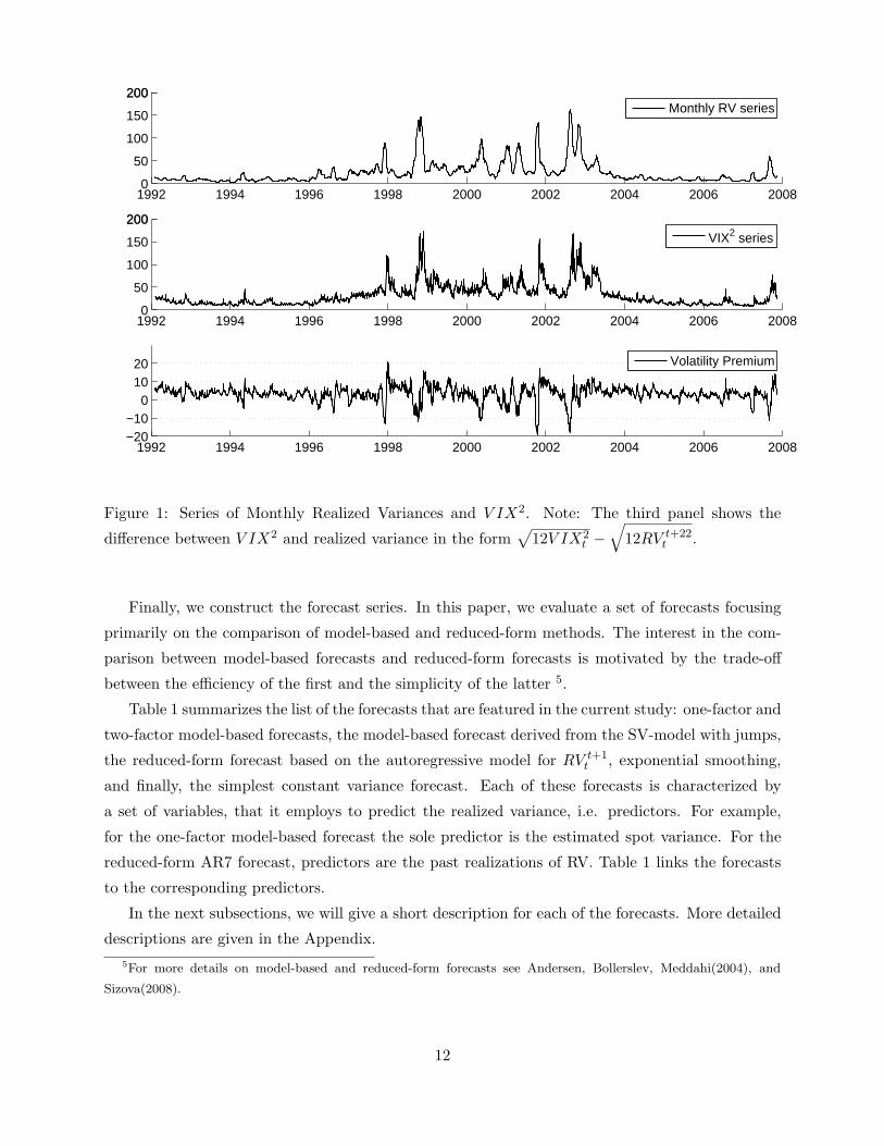
Figure 1: Series of Monthly Realized Variances and V IX2. Note: The third panel shows the

difference between V IX2 and realized variance in the form√

12V IX2t −

√12RV t+22

t .

Finally, we construct the forecast series. In this paper, we evaluate a set of forecasts focusing

primarily on the comparison of model-based and reduced-form methods. The interest in the com-

parison between model-based forecasts and reduced-form forecasts is motivated by the trade-off

between the efficiency of the first and the simplicity of the latter 5.

Table 1 summarizes the list of the forecasts that are featured in the current study: one-factor and

two-factor model-based forecasts, the model-based forecast derived from the SV-model with jumps,

the reduced-form forecast based on the autoregressive model for RV t+1t , exponential smoothing,

and finally, the simplest constant variance forecast. Each of these forecasts is characterized by

a set of variables, that it employs to predict the realized variance, i.e. predictors. For example,

for the one-factor model-based forecast the sole predictor is the estimated spot variance. For the

reduced-form AR7 forecast, predictors are the past realizations of RV. Table 1 links the forecasts

to the corresponding predictors.

In the next subsections, we will give a short description for each of the forecasts. More detailed

descriptions are given in the Appendix.5For more details on model-based and reduced-form forecasts see Andersen, Bollerslev, Meddahi(2004), and

Sizova(2008).

12

Forecasts Predictors

Model-Based SV-J Spot variance σ2t

Model-Based 2F Factors x1,t,and x2,t: σ2t = x1,t + x2,t

Model-Based 1F Spot variance σ2t

Reduced-Form AR7 RV t−i+1t−i , i = 1, 7

Exponential Smoothing RV t−i+1t−i , i ≥ 1

Random Walk RV tt−H

Table 1: Forecasts and Corresponding Predictors

5.1 Model-Based Forecasts: SV-CJ, Two-Factor and One-factor

The SV-CJ forecast is based on the model by Eraker, Johannes, and Polson (2003):

[dst

dσ2t

]=

[µ

κ(θ − σ2t )

]dt +

[σtdW s

t

σvσtdW vt

]+

[ξst

ξvt

]dJt, (27)

where dW vt and dW s

t are increments of standard Brownian motions with the correlation ρdt, Jt is

a Poisson process with the intensity λ, ξst and ξv

t are jump sizes: ξvt is exponential with the mean

1/µv, and ξst is conditionally normal with the mean µj + ρjξ

vt and the variance σ2

j . For each day

t, we estimate the model on daily close-to-close data up to t and construct the forecast of RV t+22t .

We repeat this procedure for the period of August, 2000, to October, 2007. That gives us 1780

out-of-sample monthly forecasts.

This approach is based on the daily data and disregards the intra-day information. Although

this may be seen as a drawback if the intra-day data contain extra information, this may be seen

as an advantage of the method if the intra-day data is contaminated with microstructure noise.

Moreover, taking this model to higher-frequency data may require a more elaborate dynamics, e.g.

short-term or seasonal components, see Andersen and Bollerslev (1997).

Another feature of this approach is that it separates the fast-reverting part of the variance

into the Poisson component. The rest of the variance is the slow-reverting Gaussian process σ2t .

Alternatively, the same separation of the slow-moving and fast-moving components can be achieved

by a two-factor model.

As a more elaborate alternative to SV-CJ, we will consider a two-factor model-based forecast

that employs intra-day data. To form this forecast, we assume a general two-factor ESV-model (see

Meddahi(2003)), estimate the parameters by matching the correlation structure of the variance, and

use the Kalman-filter to extract states. This procedure is not as efficient as MLE. Nevertheless, if the

model is indeed two-factor, then, regardless of the exact form of the model, this procedure delivers

the consistent estimate of EtRV t+Ht . Therefore, it is robust to certain kinds of misspecification.

13

Another alternative is a one-factor model-based forecast. It is constructed in the same way as

the two-factor model-based forecast. However, in this case, we do not disentangle fast and slow

moving components in the variance. A more detailed description of the model-based methods is

given in the Appendix.

5.2 Reduced-Form Forecasts: Autoregressive, Exponential Smoothing, and Ran-

dom Walk

From the class of reduced-form forecasts, we selected the autoregressive, exponential smoothing,

and the random walk forecasts. The autoregressive model is the projection of RV on its own past

values:

RVt+1|t = β(1)0 +

I∑

i=1

β(1)i RV t+1−i

t−i . (28)

The above model is the simplest in the class of linear models for RV. A more elaborate example is the

ARFIMA model by Andersen, Bollerslev, Diebold and Labys (2003). We chose the autoregressive

model because of its computational simplicity. Iterating the above equation, we obtain the form of

the H-period forecast:

RVt+H|t = β0 +I∑

i=1

βiRV t+1−it−i . (29)

Several prior studies have shown that the part of the realized variance coming from large jumps

in prices has a weak predictive power with respect to future variances. This finding motivated the

HAR-SV-J and the HAR-SV-CJ models by Andersen, Bollerslev, and Diebold (2007) and Andersen,

Bollerslev, Huang (2008), respectively. Here, we again choose the simplest way to improve the

forecasting power by using bi-power variations (BV) on the right-hand side of (29) instead of RV:

RVt+H|t = β0 +I∑

i=1

βiBV t+1−it−i , (30)

BV t+1t =

1/h∑

j=2

π

2|st+jh − st+jh−h| |st+jh−h − st+jh−2h|

Intuitively, BV strips off jump-components from RV that have a weak correlation with the future

dynamics of the variance. Therefore, using BV as a predictor may improve the forecasting power

of this AR model.

Exponential smoothing is a reduced-form filter for RV, that is given in the iterative form:

RVt+1|t = αRVt|t−1 + (1− α)RV tt−1,

RVt+H|t = H(αRVt|t−1 + (1− α)RV t

t−1

).

(31)

The simplest forecast out of the reduced-form forecasts is the random-walk that assumes that

“variance will not change”:

RVt+H|t = RV tt−H . (32)

14

We will compare two methods for estimation of (30) and (31), namely OLS and WLS. For instance,

for an AR-7 forecast given by (30) with I = 7, OLS estimates will minimize the sum of squared

residuals:

minβ

∑t

(RV t+Ht − β0 −

7∑

i=1

βiBV t−i+1t−i )2,

and WLS will minimize the following sum:

minβ

∑t

(RV t+Ht − β0 −

∑7i=1 βiBV t−i+1

t−i )2

wt, (33)

where the weights take the form wt = exp(γ0 +∑7

i=1 γiBV t−i+1t−i ). The exponent in the definition

of wt prevents it from turning negative. The coefficients γ0, γi are obtained through a two-step

procedure.

Note that for the SV-CJ model we use MLE. However, for the two-factor and one-factor model-

based forecasts we perform a regression in the final step (see the Appendix). Therefore, these two

forecasts will also require a choice between OLS and WLS.

6 Results

In this section we apply the economic loss-function defined in this paper towards comparison of the

following forecasts: SV-CJ, two-factor model-based, one-factor model-based, reduced-form AR-7,

exponential smoothing, and random walk. Formally, we may classify two-factor, one-factor and SV-

CJ forecasts as model-based since they approximate the conditional expectation using the model for

prices. All the other forecasts can be classified as reduced-form forecasts. We focus our attention

on the comparison of these two groups. As we vary the premium specification, we may potentially

see different rankings of these forecasts. As a conclusion, we want to determine if the difference

in the performances between these two groups is economically and statistically significant under

certain premium specifications. We also want to investigate if the ranking based on the utility-based

loss-function is drastically different from the ranking based on statistical loss-functions.

6.1 Statistical Loss-Functions

We start by assessing the statistical performance of the forecasts. To mimic the swap contract, we

consider the forecast horizon of one month. The estimation period includes the data from January,

1992. The out-of-sample performance of the forecasts is evaluated on data from August, 2000, to

October, 2007. Table 2 reports the mean-squared error, bias, mean absolute error and median

absolute error. All four are routinely used in the forecasting literature.

The lowest MSE corresponds to the SV-CJ forecast. It yields an average squared error of 50.79%,

down from 53.46% for the two-factor and down from 53.65% for the AR-7 forecasts. All the other

forecasts perform considerably less successfully. Exponential smoothing yields the smallest bias.

15

Forecasts MSE(normalized) BIAS BIAS(normalized) MAE Median AE

OLS: Model-Based 2F 53.46 % -0.46 0.027 % 11.72 6.21

OLS: Model-Based 1F 80.20 % -2.10 0.549 % 16.16 12.08

OLS: Reduced-Form AR7 53.65 % -1.30 0.211 % 11.59 6.72

OLS: Exponential Smoothing 70.28 % 0.01 0.000 % 12.06 4.46

WLS: Model-Based 2F 58.19 % 0.83 0.087 % 11.73 4.61

WLS: Model-Based 1F 84.51 % -2.25 0.633 % 12.89 6.68

WLS: Reduced-Form AR7 57.09 % -0.08 0.001 % 10.96 4.56

WLS: Exponential Smoothing 76.06 % -0.01 0.000 % 11.85 4.22

Random Walk 78.47 % 0.15 0.003 % 13.49 4.82

SV-CJ 50.79 % -1.14 0.162 % 11.55 6.84

Table 2: Statistical comparison of forecasts by the normalized MSE =∑T

t=1(RVt−RV t)2∑Tt=1(RVt−RV t)2

, bias =∑T

t=1(RV t − RV t)/T , and the normalized bias = [∑T

t=1(RV t−RV t)/T ]2

[∑T

t=1(RVt−RV t)2/T ], where RV t is the sample

average of the realized variances, and RV t is the forecast. MAE is the sample average of the

absolute errors |RV t −RV t|.

Both MAE and Median AE, measures that put less weight on large errors compared to MSE,

favor reduced-form forecasts: AR-7 and exponential smoothing respectively. Comparing this rank-

ing to the one based on MSE, we conclude that the first rank of the SV-CJ forecast by MSE may

be explained by several large errors admitted by reduced-form forecasts.

Overall, based on statistical loss functions, the performances of the reduced-form and model-

based forecasts are quite close. The model-based forecasts lead in MSE, and the reduced-form

forecasts lead in MAE and MedAE measures. In the next subsection, we ask if the results from the

statistical comparison carry over to economic loss-functions.

6.2 Economic Loss-Functions for Constant Trader’s Risk Premium

The simplest benchmark case is the one with a constant premium πt = π(α) that increases with the

risk-aversion parameter α. For simplicity and without loss of generalization, we may parameterize

the trader’s premium to be πt = α. For each choice of α and a forecasting system, we form trading

activity of the variance swap seller and calculate the corresponding utility. Figure 2 shows sample

average utilities corresponding to several forecasting systems. Axis X in Figure 2 corresponds to

the risk-aversion of the trader measured in volatility premium units, i.e. it is approximately the

sample average of√

3πt . The risk-aversion of the trader in its classical form grows from the left to

the right. Utilities are normalized by the average price of the contract, thus they can be interpreted

in a compensation manner. For example, consider a trader who demands a volatility premium of

16

1% on average, i.e. the mean of√

12Pt −√

12EtRVt+H

t is equal to 1. If he trades always (i.e.

It = 1, ∀t), then his average utility is around 20.0%. If he never trades (i.e. It = 0, ∀t), then his

average utility is zero. Therefore, he will be willing to pay up to 20 % of the contract price to be

able to participate in the trade.

There are five lines in the figure that are utilities derived from employing a two-factor model-

based forecast, one-factor model-based forecast, SV-CJ model-based forecast, AR-7 reduced-form

forecast, and the strategy of “trading always”, i.e. always agreeing to trade. All the forecasts are

calculated using weighted least-squares, as their OLS versions perform uniformly weaker.

Figure 2 can be divided into three regions. In the first region the seller would prefer to trade

always, because the utility from this strategy exceeds the maximum utility from strategies based on

forecasting. That is, in this region forecast errors prevent sellers from carrying out profitable trades,

rather than alerting them against future high uncertainty in the market. This region lies below the

risk-aversion with the volatility premium of 2%, implying that a nearly risk-neutral trader derives

no advantage from using statistical forecasts.

The second region, above 10%, is the region where the market volatility premium is not high

enough to encourage betting on volatility. In this region, traders can be better off by declining to

be on the sell side of the variance swap trade. In this region, forecast errors push forecasters into

risky trading when they would be better off by refraining from participation altogether.

Finally, the most interesting region, that lies between 2% and 10% is the region where the

variance seller profits from forecasting. In this region, the reduced-form forecast (solid dark line)

uniformly dominates all the other forecasts. The forerunner is the two-factor model-based forecast,

which employs high-frequency data. Other forecasts also result in positive gains. The point at

which the trader is willing to pay the highest fees for forecasts is at around 3.5 % of the trader’s

volatility premium. At this point, the trader is indifferent between always participating in trading

and never participating, and the compensation for the access to statistical forecasts reaches 7%

(AR-7 forecast).

It follows from Figure 2 that out of three depicted model-based forecasts the one that is based

on high-frequency data and incorporates two components in the variance is the most successful.

SV-CJ also includes a pair of volatility components (the Gaussian part and the Poisson part) but is

based on daily data. One-factor forecast performs the worst despite using the high-frequency data,

which is in accordance with prior research on the performance of one-factor models for long-term

forecasting, see Sizova(2008).

17

0 1 2 3 4 5 6 7 8 9 10 11−5

0

5

10

15

20

25

Trader’s Risk Aversion (volatility premium units)

Util

ity (

% o

f con

trac

t pric

e)

Model−Based Forecast: 2−FactorModel−Based Forecast: 1−FactorModel−Based Forecast: SV−CJReduced−Form Forecast: AR−7Always Trade

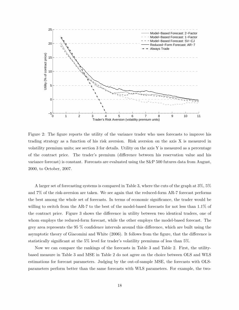
Figure 2: The figure reports the utility of the variance trader who uses forecasts to improve his

trading strategy as a function of his risk aversion. Risk aversion on the axis X is measured in

volatility premium units; see section 3 for details. Utility on the axis Y is measured as a percentage

of the contract price. The trader’s premium (difference between his reservation value and his

variance forecast) is constant. Forecasts are evaluated using the S&P 500 futures data from August,

2000, to October, 2007.

A larger set of forecasting systems is compared in Table 3, where the cuts of the graph at 3%, 5%

and 7% of the risk-aversion are taken. We see again that the reduced-form AR-7 forecast performs

the best among the whole set of forecasts. In terms of economic significance, the trader would be

willing to switch from the AR-7 to the best of the model-based forecasts for not less than 1.1% of

the contract price. Figure 3 shows the difference in utility between two identical traders, one of

whom employs the reduced-form forecast, while the other employs the model-based forecast. The

grey area represents the 95 % confidence intervals around this difference, which are built using the

asymptotic theory of Giacomini and White (2006). It follows from the figure, that the difference is

statistically significant at the 5% level for trader’s volatility premiums of less than 5%.

Now we can compare the rankings of the forecasts in Table 3 and Table 2. First, the utility-

based measure in Table 3 and MSE in Table 2 do not agree on the choice between OLS and WLS

estimations for forecast parameters. Judging by the out-of-sample MSE, the forecasts with OLS-

parameters perform better than the same forecasts with WLS parameters. For example, the two-

18

Forecasts 3% 5% 7%

OLS: Model-Based 2F 5.381 % 1.369 % 0.846 %

OLS: Model-Based 1F 5.538 % -0.280 % -3.702 %

OLS: Reduced-Form AR7 7.089 % 2.466 % 1.764 %

OLS: Exponential Smoothing 5.665 % 0.870 % 0.059 %

WLS: Model-Based 2F 6.136 % 2.416 % 1.719 %

WLS: Model-Based 1F 6.684 % 1.313 % -0.981 %

WLS: Reduced-Form AR7 7.714 % 3.551 % 2.882 %

WLS: Exponential Smoothing 6.857 % 1.648 % 0.432 %

Random Walk 2.967 % -1.745 % -1.411 %

SV-CJ 5.633 % 1.517 % 1.440 %

Always trade 4.045 % -14.178 % -34.261 %

Table 3: Table reports utility of the variance trader for different levels of risk-aversion in volatility

premium units (see section 3). The utilities are expressed as percentages from the contract price.

Rows correspond to different forecasts that are used to form optimal trading strategies.

factor model-based forecast yields the MSE of 58.19% and 53.46% for WLS and OLS estimators,

respectively. This result is expected, as OLS parameters are found through the minimizing of

squared residuals in-sample, what translated into the minimizing of squared residuals out-of-sample.

However, for the utility-based loss function, WLS-versions of forecasts perform better for all levels of

risk aversion. For example, at trader’s volatility premiums of 7% the trader is willing to pay around

0.9% of the contract price to switch from using the OLS-type two-factor model-based forecast to

the WLS-type forecast.

Utility-based and MSE rankings disagree on the performance of the SV-CJ model. This forecast

is the most efficient based on MSE, but loses to the reduced-form forecast based on the utility-based

performance measure. Overall, median absolute error seems to give the ranking that is the closest

0 2 4 6 8 10−1

0

1

2

3

4

Trader’s Risk Aversion (volatility premium units)

∆ U

=

Util

ity(A

R−

7)

− U

tility

(2−

Fa

cto

r)

Figure 3: The difference between average

utilities for the reduced-form AR-7 and the

model-based two-factor forecasts. Grey

area denotes the 95 % confidence interval.

19

m 1 2 3 1 2 3

x1t < 0 x1t > 0

β0 2.68(0.33)

5.91(0.68)

9.77(0.65)

2.46(0.12)

6.20(0.23)

10.52(0.35)

β1 10.03(5.52)

15.81(8.46)

17.27(17.18)

1.03(0.24)

0.69(0.37)

−0.16(0.83)

β2 40.34(24.94)

63.67(42.51)

51.83(106.88)

−0.25(0.11)

−0.02(0.15)

0.36(0.35)

β3 57.15(32.35)

92.00(59.44)

65.74(154.20)

0.03(0.01)

3e−3

(0.01)−0.03(0.04)

Table 4: The table reports the estimates of coefficients in the formula (34). The model was estimated

in-sample for the years of 1992-2007 using non-linear least squares. Newey-West standard errors

are shown in parenthesis.

to the one based on the trader’s utility. The property that possibly links these two measures is the

robustness to outliers.

Note that the utility-based loss-function from this section is still quite close to the statistical

measures, since it assumes that the risk of the transaction is not changing over time. The next step

is to consider more natural specifications for the trader’s premium, where the premium is related

to the current uncertainty about the future variance.

6.3 Economic Loss-Function for Variable Risk Premiums

To define the premium in this section, we construct a proxy for the conditional moments of realized

variance Et|RV t+Ht −EtRV t+H

t |m using the two-factor model-based forecast for EtRV t+Ht and then

fitting an exponential model of the form:

Et|RV t+Ht − EtRV t+H

t |m = eβ0+β1x1,t+β2x21,t+β3x3

1,t , (34)

where x1t is the estimated slow-reverting component of volatility from the two-factor model. ( See

the Appendix.) Table 6.3 reports resulting the coefficients.

Although there are many possible ways to specify this proxy, e.g. casting it within the reduced-

form forecast framework, the two-factor model-based offers certain simplifications. Within this

framework, all the conditional moments are the functions of only two states, x1t and x2t. The

choice was motivated mostly by simplicity of including higher orders of the regressor x1,t into

the formula. Note, that x2,t is not included, as the slopes on this component were found to be

insignificant. The exponent in (34) ensures that the trader’s premium is positive.

Subsequently, we varied the two parameters m ∈ 1, 2, 3 and n ≥ 1m to collect a set of premiums

πt = αKm+n−1[Et

∣∣∣RV t+Ht −RVt+H|t

∣∣∣m]n

. We start with the quadratic-utility case for m = 2 and

20

n = 1, and report the results for other premium specifications in the Appendix.

Figure 4 shows average utilities that result from trading strategies based on different forecasting

systems. As in the case of the constant premium, the X axis in Figure 4 corresponds to the risk-

aversion of the trader measured in volatility premium units, i.e. it is approximately the sample

average of√

3πt . Risk-aversion increases from the left to the right. Unlike the constant premium

case, the risk-aversion depends not only on the preferences of the trader, but also on the size of the

contract K: πt = πt(α, K). This variance premium is strictly increasing in α and the notional K.

Therefore the utility patterns across different values on the X axis have a dual interpretation: on

the one hand they can be interpreted as utilities of traders with different absolute risk-aversions,

on the other hand they can be interpreted as utilities of the same trader for different contract sizes,

that are exogenously given by the hedging demands of a buyer.

Similar to the case of a constant trading premium, the graph can be divided into three areas.

The first one is the area where traders should prefer to trade regardless of their forecasts. This

area lies below the 0.9% level of the trader’s volatility premium. The second area, above 12% of

the volatility premium, is the area where they should always hedge their position. The area where

forecasts bring substantial profits to the trader lies between these two marks.

The utility from using statistical forecasts increased for all levels of risk-aversion and all the

forecasts, with the exception of the one-factor model-based forecast. Now the maximum value from

forecasting is reached at trader’s volatility premium of 2.4 % and is above 10 % of the contract

price (for AR-7 forecast). The weakest of the presented forecasts – the one-factor forecast – is still

informative for the trader yielding positive profits for risk aversions of less than 4%. Interestingly,

for the premium that changes with uncertainty in the market, the two-factor model-based forecast

has a clear advantage in comparison to the SV-CJ, which employs only daily data, and to the

simpler one-factor model.

From Figure 4 it follows that for the quadratic utility case, the two-factor model-based and

reduced-form forecasts perform equally well. In terms of their comparative performance, the

reduced-form forecast is slightly better for less risk-averse traders or alternatively, for smaller sizes

of contracts, and the model-based forecast is slightly better in the opposite case of high risk-aversion

and larger contract sizes. The threshold lies at around 4% of the volatility premium.

21

0 1 2 3 4 5 6 7 8 9 10 11−5

0

5

10

15

20

25

Trader’s Risk Aversion (volatility premium units)

Util

ity (

% o

f con

trac

t pric

e)

Model−Based Forecast: 2−FactorModel−Based Forecast: 1−FactorModel−Based Forecast: SV−CJReduced−Form Forecast: AR−7Always Trade

Figure 4: The figure reports the utility of the variance trader who uses forecasts to improve his

trading strategy as a function of his risk aversion. Risk aversion on the axis X is measured in

volatility premium units; see section 3 for details. Utility on the axis Y is measured as a percentage

of the contract price. The trader’s premium (difference between his reservation value and his

variance forecast) is proportional to the conditional variance VartRV t+22t . Forecasts are evaluated

using the S&P 500 futures data from August, 2000, to October, 2007.

Table 5 reports the results for the whole set of forecasts at certain values of risk-aversion. Among

the reduced-form forecasts, exponential smoothing performs the best for all three columns. It is

the best among all the forecasts for lower risk-aversion, and yields less than 0.25% of the contract

price to the two-factor model-based forecast for higher risk-aversions.

Therefore, we found that for the risk-premium πt that is proportional to the current uncertainty

in the market, the comparison between reduced-form forecasts and model-based forecasts depends

on the risk-aversion of the trader. In particular, for smaller risk-aversions, AR-7 and exponential

smoothing dominate the two-factor model-based forecast, but for larger risk-aversions they yield

respectively up to 0.2% and 0.5% of the contract price. This outcome is different from the case of

the constant πt, under which the reduced-form forecast was uniformly better than the two-factor

model-based forecast.

Figure 5 explains the difference between the cases of the constant πt and the variable πt. The

figure reports the averages of the trade indicator It, cash flows Ct, and utilities ut within seven

22

Forecasts 3% 5% 7%

OLS: Model-Based 2F 4.090 % 2.524 % 0.730 %

OLS: Model-Based 1F -4.923 % -3.329 % -1.705 %

OLS: Reduced-Form AR7 2.407 % 1.207 % -0.037 %

OLS: Exponential Smoothing 3.561 % 1.483 % 0.471 %

WLS: Model-Based 2F 6.899 % 4.149 % 2.243%

WLS: Model-Based 1F 2.141 % 0.403 % -0.160 %

WLS: Reduced-Form AR7 7.158 % 3.757 % 1.874 %

WLS: Exponential Smoothing 7.178% 3.973 % 1.959 %

Random Walk 3.157 % 2.033 % 2.193 %

SV-CJ 4.234 % 1.915 % 1.156 %

Always trade -9.122 % -39.655 % -32.723 %

Table 5: Table reports utility of the variance trader for different levels of risk-aversion in volatility

premium units (see section 3). The utilities are expressed as percentages from the contract price.

Rows correspond to different forecasts that are used to form optimal trading strategies.

equally-sized periods between August, 2000, and October, 2007. During this period, the first

four years 2000-2003 are characterized by high volatility. (See Figure 5.) The following years of

2004-2006 were relatively stable.

The first two panels of Figure 5 show how often the trader participated in selling swaps during

each year. Note that under quadratic utility, the probability to trade in low-uncertainty times is

higher than the same probability in times of high uncertainty. Thus, the variable premium down

weights periods with high volatility and puts more weight on low volatility periods. Intuitively,

traders will avoid trading in the turbulent years, and will participate in trade during the less volatile

years even though the market may offer them moderate expected profits.

The second and the third pairs of panels in Figure 5 report two alternative measures of the

success for the forecasts: average cash-flows and utilities. Note that the reduced-form forecast is

better for the periods with high uncertainty and slightly worse in the periods with low uncertainty.

Thus, for the variable premium the advantage from using the reduced-form forecast disappears

as the importance of the first part of the sample diminishes. The higher the risk aversion of the

trader, the less chance that the trader will trade in the high-uncertainty times. Hence, eventually

the model-based forecast will become slightly better, as the only period that will matter for the

forecaster will be the years of 2004 - 2006.

23

2001 2002 2003 2004 2005 2006 2007 20080

0.2

0.4

0.6

0.8

1Number of Trades: Constant Risk Premium

2001 2002 2003 2004 2005 2006 2007 20080

0.2

0.4

0.6

0.8

1Number of Trades: Quadratic Utility

2001 2002 2003 2004 2005 2006 2007 20080

5

10

15

Average Cash−Flows: Constant Risk Premium

2001 2002 2003 2004 2005 2006 2007 20080

5

10

15

Average Cash−Flows: Quadratic Utility

2001 2002 2003 2004 2005 2006 2007 2008−10

0

10

20

30

40Average Utility: Constant Risk Premium

2001 2002 2003 2004 2005 2006 2007 2008−10

0

10

20

30

40Average Utility: Quadratic Utility

Model−Based Reduced−Form

Figure 5: Performance of Forecasts across Years

Note: Panels in the first row report trading intensities 1T

∑Tt=1 It. Panels in the second row report average cash flows

1T

∑Tt=1 Ct. Panels in the third row report average utilities 1

T

∑Tt=1 ut normalized by the contract price. Graphs show the

averages across 7 periods starting August 2000 and ending in October 2007. Gray plots are for trading intensities, cash flows

and utilities of the trader who employs the two-factor model-based forecast. Black plots are for the AR-7 reduced-form

forecast.

Several robustness checks are presented in the Appendix. First, we show that the results of this

section hold for the “classic” quadratic preferences as given by (8). Second, we report the forecast

comparison for other choices of the premium parameters.

To summarize our results for the quadratic utility, the performances of the reduced-form fore-

casts and model-based forecasts for variable trader’s premium are very close. The reduced-form

forecast is still better for moderate risk aversions. The dependence of the winning forecast on

the risk aversion suggests that none of the forecasts can successfully model the difference in the

dynamics between low volatility and high volatility periods.

24

7 Simulation Study

In this section we reproduce the results of the forecast comparison on simulations with the SV-CJ

dynamics by Eraker, Johannes, and Polson (2003). The SV-CJ model was used to form one of

the model-based forecasts in the previous section. Under this model the process for log-prices st is

described by the next system of equations:[

dst

dσ2t

]=

[µ

κ(θ − σ2t )

]dt +

[σtdW s

t

σvσtdW vt

]+

[ξst

ξvt

]dJt. (35)

The parameters for simulations were estimated on the daily S&P 500 futures returns over the sample

of 1992 - 2007, and take the following values: mean return µ = 0.032, volatility mean-reversion

k = 0.0216, mean variance θ = 0.730, variance parameter of volatility σ2v = 0.0178, jump intensity

λ = 0.012, and the leverage effect ρ = −0.725. Also, jumps in the variance ξvt are distributed

exponentially with the parameter µv = 2.09, and jumps in returns ξst are conditionally normal

N(µj + ρjξvt , σ2

j ), where µj = −0.995, ρj = −1.52, and the variance of jumps σ2j is equal to 2.66.

The data was simulated using the Euler discretization scheme at one second frequencies. From

one-second log-prices we constructed 5-minute returns. As in the observed data, each trading day

in these simulations lasts for 6.5 hours, plus one overnight return. For simplicity, the distribution

of the overnight returns is the same as for 5-minute day-time returns. Simulations include 5 data

sets each of a length of 4000 days, that is approximately equal to 5 times 16 years. Additionally, we

simulated 60000-day series to estimate the reduced-form model for the realized variance: vector-

autoregression for RV and BV. Table 8 in the Appendix reports the estimates of the reduced-form

model.

To form the model-based forecast from (35) we take the parameters of the model as given and

use particle filtering to extract the monthly RV forecasts. To form close-to-close V IX2-series, we

estimated the following HAR-model on observed data that links V IX2 to past realized variance

over different horizons:

V IX2t = β0 +

5∑

i=1

βiRV t−i+1t−i + βmonRV t

t−20 +3∑

i=1

βqrti RV

t−60(i−1)t−60i (36)

The resulting R2 of the above regression is 82.6%. In simulations, V IX2 was constructed using

formula (36) with the estimates reported in Table 9 in the Appendix.

Similar to the observed data, we asses the performance of the model-based forecast and the

reduced-form forecast, first using statistical measures, and then the new utility-based measure.

The statistical performance of the forecasts is reported in Table 6. The utilities derived from

application of the same forecasts are shown in Figure 6. By statistical performance, the model-

based forecast is slightly leading, giving the minimum of MSE (45.02%), MAE (7.26) and Median

AE (5.42). The model-based forecast under no misspecification is the most efficient by construction,

25

but the difference from the reduced-form forecast is minimal. The reduced-form forecast yields the

MSE of 46.13 %, MAE of 7.44 and Median AE of 5.66.

Table 6: Statistical Performance of Variance Forecasts for Simulated Data: True Model

MSE MAE Median AE

Reduced-Form 46.13% 7.44 5.66

Model-Based 45.02% 7.26 5.42

Note: Table reports MSE =∑T

t=1(RVt−RV t)2

∑Tt=1(RVt−RV t)2

, Mean AE = 1T

∑Tt=1 |RVt − RV t|, and Median AE statistics for the reduced

form forecast based on VAR, and the forecast based on the model (35). The data consists of five simulations from the same

model (35) of the length 4000 days each.

Figure 6 shows the utilities for different risk-aversions of the variance trader derived from using

the model-based and the reduced-form forecasts. These two graphs visibly coincide both in Panel

A, for the constant risk premium, and in Panel B, for the quadratic utility.

26

0 1 2 3 4 5 6 7 8 9 10 11−5

0

5

10

15

20

25A. Constant Premium

Risk Aversion (volatility premium units, %)

Util

ity (

% o

f con

trac

t pric

e)

Model−Based SVCJReduced−FormAlways trade

0 1 2 3 4 5 6 7 8 9 10 11−5

0

5

10

15

20

25B. Quadratic Utility

Risk Aversion (volatility premium units, %)

Util

ity (

% o

f con

trac

t pric

e)

Model−Based SVCJReduced−FormAlways trade

Figure 6: Utility-Based Comparison of Variance Forecasts for Simulated Data : True Model

Note: The figure reports the utility of the variance trader who uses forecasts to improve his trading strategy as a function of

his risk aversion. Risk aversion on the X axis is measured in volatility premium units. (See section 3 for details.) Utility on

the Y axis is measured as a percentage of the contract price. In Panel A, the trader’s premium (the difference between his

reservation value and his variance forecast) is constant; in Panel B, the premium is proportional to the conditional variance

VartIV t+Tt that is calculated using the true model (35). The data for this figure was simulated from the SV-CJ model (35)

and consists of 5 data sets of the length 4000 days.

To summarize, if prices follow the SV-CJ dynamics and are observed at 5-minute intervals, then

the reduced-form forecast performs very close to the most efficient model-based forecast in terms

of MSE and other statistical measures. The same holds for the utility-based loss-function; for each

level of the trader’s risk aversion, utilities derived from using the reduced-form forecast almost

coincide with the utilities derived from the efficient forecast based on the true model. Therefore,

the reduced-form forecast,which does not make any assumptions about the underlying process for

returns and is ultimately simple to construct, practically attains the maximum efficiency among all

the possible forecasts.

27

7.1 Simulated with Misspecification

To see why the model-based approach may eventually fail in comparison to the reduced-form one,

we expand the original model by adding a new component to the variance v2,t that has a higher

mean-reversion than the original variance. Thus, the new model includes three components – two

Gaussian ones and one that is a Poisson jump:

dst

dv1,t

dv2,t

=

µ

κ(θ − v1,t)

κ2(θ − v2,t)

dt +

√v1,t + v2,tdW s

t

σv√

v1,tdW vt

σv,2√

v2,tdW vt

+

ξst

ξvt

0

dJt, (37)

where κ2 = 1.5. We specify the other parameters as in the original model, and pick the volatility-

of-volatility parameters in such a way that σ2v/κ = σ2

v,2/κ2. Finally, the return data are adjusted

by a scalar to ensure that the average market volatility premium is equal to 3.23%, as in the data

for the S&P 500 and VIX.

To construct the model-based and the reduced-form forecast, we use 60000 days of simulated

data to estimate the parameters of the SV-CJ model and vector auto-regression (VAR) for RV and

BV. Second, we generate five data sets of the length 4000 days, and form 3878 forecasts based on

the SV-CJ model that employs 5-minute returns, reduced-form forecasts, VIX series and actual

monthly RV series.

The results of the statistical performance of the forecasts are presented in Table 7. This table

demonstrates that inclusion of the additional fast-reverting component in the variance, that is not

a jump, “confuses” the model-based forecast, so it performs much worse in comparison to the

case with no misspecification (70.27% MSE vs. 45.02% MSE) and also in comparison with the

reduced-form forecast (54.75% MSE). The same is true for the mean and median absolute errors.

Table 7: Statistical Performance of Variance Forecasts For Simulated Data: Misspecified Model

MSE MAE Median AE

Reduced-Form 54.75% 3.91 3.06

Model-Based 70.27% 5.04 4.66

Note: Table reports MSE =∑T

t=1(RVt−RV t)2

∑Tt=1(RVt−RV t)2

, Mean AE = 1T

∑Tt=1 |RVt − RV t|, and Median AE statistics for the reduced

form forecast based on VAR for RV and BV, and the forecast based on the model (35). The data consists of five data sets

simulated from the model (37) of 4000 days each.

Figure 7 shows the results of the utility-based comparison. In contrast to the case when we

constructed the forecast based on the true model, in Figure 7 we see that now there is a difference

in performance between the reduced-form and the model-based forecasts; for lower risk-aversions

28

the reduced-form forecast is about 2.5 % better than the model-based forecast. This difference

vanishes as the risk-aversion increases.

0 1 2 3 4 5 6 7 8 9 10 11−5

0

5

10

15

20

25A. Constant Premium

Risk Aversion (volatility premium units, %)

Util

ity (

% o

f con

trac

t pric

e)

Model−Based SVCJReduced−FormAlways trade

0 1 2 3 4 5 6 7 8 9 10 11−5

0

5

10

15

20

25B. Quadratic Utility

Risk Aversion (volatility premium units, %)

Util

ity (

% o

f con

trac

t pric

e)

Model−Based SVCJReduced−FormAlways trade

Figure 7: Utility-Based Comparison for Simulated Data : Misspecified Model

Note: The figure reports the utility of the variance trader who uses forecasts to improve his trading strategy as a function of

his risk aversion. Risk aversion on the X axis is measured in volatility premium units. (See section 3 for details.) Utility on

the Y axis is measured as a percentage of the contract price. In Panel A, the trader’s premium (the difference between his

reservation value and his variance forecast) is constant; in Panel B, the premium is proportional to the conditional variance

VartIV t+Tt that is calculated using the true model (37). The data consists of five data sets simulated from the model (37) of

the length 4000 days. Model-based forecast is calculated using the SV-CJ model (35).

Note also that the utility patterns in Panels A and B are very similar and qualitatively the same.

The reason for this similarity is that the data simulated from (37) does not exhibit clear periods of

large and low volatility. The next logical step would be to consider the model with regime-switching,

that could give this property, e.g. as in the paper by Poon, Hyung and Granger(2006).

Summarizing this section, we can conclude that for a correctly specified model,the reduced-form

forecast performed very close to the model-based forecast that is the most efficient by construction.

Furthermore, in the case of misspecification, it outperformed the model-based forecast both for

statistical and utility-based measures.

29

8 Conclusion

We proposed a new variance forecast loss-function based on variance trading. In contrast to con-

ventional forecast performance measures, the suggested loss-function evaluates the performance of

a forecast versus information that is already included in the market prices.

We showed that the performance measure that is relevant for designing trading strategies is

state-dependant. In particular, it puts less weight on the forecast errors during periods of turmoil.

For this new loss function, we examined the out-of-sample performances of reduced-form and

model-based forecasts for variances of the S&P 500. We demonstrated that a simple reduced-form

forecast is not outperformed by more sophisticated techniques, such as model-based forecasts. This

paper demonstrates this fact for utility-based loss-functions.

Regarding the differences between statistical and utility-based measures, we found that for

utility-based measures, the performance of the reduced-form forecast vs. the model-based approach

may be improved even further by using non-linear techniques that may be more successful in

capturing the difference in variance dynamics during periods of high and low uncertainty.

References

[1] Andersen, T.G. and T. Bollerslev (1997), “Intraday Periodicity and Volatility Per-

sistence in Financial Markets”, Journal of Empirical Finance, 4, 115-158.

[2] Andersen, T.G. and T. Bollerslev (1998), “Answering the Skeptics: Yes, Standard

Volatility Models do Provide Accurate Forecasts”, International Economic Review,

39/4, 885-905.

[3] Andersen, T.G., T. Bollerslev, P.F. Christoffersen and F.X. Diebold (2005), “Volatil-

ity Forecasting”, Working Paper, NBER .

[4] Andersen, T., Bollerslev, T., Diebold, F.X. and Labys, P. (2003), “Modeling and

Forecasting Realized Volatility”, Econometrica, 71, 529-626.

[5] Andersen, T.G., T. Bollerslev, and F.X. Diebold (2007)

[6] Andersen, T.G., T. Bollerslev, and N. Meddahi (2004), “Analytical Evaluation of

Volatility Forecasts”, International Economic Review, 45, 1079 - 1107.

[7] Andersen, T.G., T. Bollerslev, and X.Huang(2008)

[8] Barndorff-Nilsen, O.E. and N. Shephard (2002), “Econometrics Analysis of Realized

Volatility and Its Use in Estimating Stochastic Volatility Models”, Journal of Royal

Statistical Society, 109, 33 - 65.

30

[9] Bollerslev, T. and H. Zhou (2006), “Volatility puzzles: a simple framework for gaug-

ing return-volatility regressions,” Journal of Econometrics, 131,123150.

[10] Bollerslev, T., H. Zhou, and G. Tauchen(2008), “Expected Stock Returns and Vari-

ance Risk Premia,” Review of Financial Studies, forthcoming

[11] Carr, P. and L. Wu, “Variance Risk Premia”, Review of Financial Studies, forthcom-

ing.

[12] Corsi, F.(2004), “A Simple Long Memory Model of Realized Volatility”, Manuscript.

[13] Drechsler I. and A. Yaron, ”What’s Vol Got To Do With It,”Manuscript, the Whar-

ton School, University of Pennsylvania.

[14] Eraker, B. (2008), “The Volatility Premium,” Manuscript, Duke University.

[15] Eraker, B., M.Johannes, and N.Polson (2003), “The Impact of Jumps in Volatility

and Returns ”, The Journal of Finance, 8, 1269 - 1300.

[16] Eun, Ch.S. and B.G. Resnick(1984), “Estimating the Correlation Structure of Inter-

national Share Prices”, The Journal of Finance, 39/5, 1311-1324.

[17] Figlewski, S. and U. Thomas (1983), “Optimal Aggregation of Money Supply Fore-

casts: Accuracy, Profitability, and Market Efficiency”, Journal of Finance, 38, 695-

710.

[18] Giacomini, R. and H. White(2006),“Test of Conditional Predictive Ability”, Econo-

metrica, 74/6, 1545 - 1578.

[19] Guo H. (2006), “On the Out-of-Sample Predictability of Stock Market Returns”,

Journal of Business, 79, 645 - 670.

[20] Huang, C.F. and R.H. Litzenberger (1988), “Foundations for financial economics”,

New York.

[21] Johannes, M., A. Korteweg, and N. Polson (2008), “Sequential learning, predic-

tive regressions, and optimal portfolio returns”, Manuscript, University of Chicago,

Graduate School of Business.

[22] Johannes, M., N. Polson, and J. Stroud (2003), “Sequential optimal portfolio perfor-

mance: Market and volatility timing”, Manuscript, University of Chicago, Graduate

School of Business.

31

[23] Kirby, Ch., J. Flemming,and B. Ostdiek (2003), “The economic value of volatility

timing using “realized” volatility”,Journal of Financial Economics 67, 473-509.

[24] Kirby, Ch., J. Flemming,and B. Ostdiek (2001), “The economic value of volatility

timing”, Journal of Finance 56, 329-352.

[25] Leitch G. and J.E. Tanner (1991),“Economic Forecast Evaluation:Profits Versus the

Conventional Error Measures”, The American Economic Review, 81/3, 580.

[26] Meddahi, N.(2003), “ARMA Representation of Integrated and Realized Variances”,

Econometrics Journal, 6, 334 - 355.

[27] Patton A., and A. Timmermann (2007), “Testing Forecast Optimality under Un-

known Loss”, Journal of the American Statistical Association, 102(480), 1172-1184.

[28] Poon, S.H., N. Hyung, and C.W. Granger (2006), “The Source of Long Memory in

Financial Market Volatility”, in Rapach D.E. and M.E. Wohar ed. “Forecasting in the

Presence of Structural Breaks and Model Uncertainty”, Elsevier Series, forthcoming

[29] Sizova, N.(2008), “Integrated Variance Forecasting: Model-Based vs. Reduced-

Form”, Job Market Paper, Duke University.

[30] Tauchen, G.(2004), “Recent Developments in Stochastic Volatilility: Statistical Mod-

elling and General Equilibrium Analysis”, Manuscript, Duke University.

[31] Todorov, V.(2007a), “Estimation of Continuous-Time Stochastic Volatility Models

with Jumps using High-Frequency Data”, Manuscript, Duke University.

[32] Todorov, V.(2007b), “Variance Premium Variance Dynamics”, Manuscript, Duke

University.

[33] West, K.D., Edison, H.G., and D. Cho (1993), “A utility-based comparison of some

models of exchange rate volatility”, Journal of International Economics, 35, 23-45.

A SV-CJ Model-Based Forecast

The SV-CJ forecast is based on the following model:

[dst

dσ2t

]=

[µ

κ(θ − σ2t )

]dt +

[σtdW s

t

σvσtdW vt

]+

[ξst

ξvt

]dJt,

32

where dW vt and dW s

t are increments of standard Brownian motions with the correlation ρdt, Jt is

a Poisson process with the intensity λ, ξst and ξv

t are jump sizes: ξvt is exponential with a mean

1/µv, and ξst is conditionally normal with a mean µj + ρjξ

vt and the variance σ2

j .

For each day t, we estimate the system above on daily close-to-close data using the MCMC

method described in Eraker, Johannes, Polson (2003) and data up to the day t. In this method

we generate draws of parameters, jumps and variances from their conditional distributions given

the observed data. Then, at each draw we also generate the realized variance of the future return

RV t+22t . The average across draws gives us the expectation of the future realized variance given

the observed daily returns up to day t. Figure 8 reports the estimated parameter values as they

evolve with time.

2001 2002 2003 2004 2005 2006 2007 20080.02

0.04

µ

2001 2002 2003 2004 2005 2006 2007 20080.015

0.020.025

0.030.035

κ

2001 2002 2003 2004 2005 2006 2007 20080.6

0.8

1

θ

2001 2002 2003 2004 2005 2006 2007 20080.015

0.02

0.025

σv2

2001 2002 2003 2004 2005 2006 2007 2008

0.01

0.02

λ

2001 2002 2003 2004 2005 2006 2007 2008

−1

−0.5

µ

j

2001 2002 2003 2004 2005 2006 2007 2008−2

−1.8

−1.6

ρj

2001 2002 2003 2004 2005 2006 2007 20082.62.8

33.2

σj2

2001 2002 2003 2004 2005 2006 2007 20081.6

1.7

1.8

µv

2001 2002 2003 2004 2005 2006 2007 2008

−0.7

−0.6

ρ

Figure 8: Estimated Parameter Values for the SV-CJ model

33

B One/Two-Factor Model-Based Forecasts

N.Meddahi (2001) demonstrated that each SV-model for log-prices st with square-integrable vari-

ances σ2t = σ2

t (xt) can be represented by an ESV-model:

dst = µtdt + σ(xt)dW st

σ2(xt) = a0 +p∑

i=1

aixit (38)

dxit = −kixitdt + φi(xit)dWit, i = 1, p

E(xitxjt) = I(i = j)

where xt = x1t, ..., xpt are referred to as factors. The above definition implies that the spot vari-

ance σ2(xt) can be represented by a sum of unconditionally uncorrelated autoregressive processes.

After small corrections for usually negligible drifts in intra-day returns, the forecast of the future

realized variance can be obtained for ESV-models in the following form:

EtRV t+Ht ≈ a0H +

p∑

i=1

1− e−kiH

kixi,t (39)

Factors xt are not observable but can be estimated. The same holds for parameters a0 and ki,

i ∈ 1, p. It appears that we can form the forecast (39) using methods that do not rely on the

specification of volatility-in-volatility terms φi(), and the correlation between returns and variances,

i.e. corr(dWit, dW st ). The suggested method is not as efficient as MLE, but it is to some extent

robust to misspecification. The only parameter that is crucial to define is the number of factors p

and we will fix it to be p = 1 for the one-factor forecast, and p = 2 for the two-factor forecast.

The outline of the techniques we will use to estimate the model (38) and form the forecast is as

follows. First, we will use GMM based on the correlation structure of the bi-power variations BV

similar to Todorov (2007) and then use the Kalman filter to filter the states xt. Bi-power variation

is defined as

BV t+1t =

1/h∑

j=2

π

2|st+jh − st+jh−h| |st+jh−h − st+jh−2h| .

For estimation, we matched the covariances of the integrated variance IV t+1t ≡ ∫ t+1

t σ2sds that

can be derived based on the model (38):

cov[IV t+1t , IV t+l+1

t+l ] =p∑

i=1

a2i

[1− eki

ki

]2

e−ki(l−1), ∀l ∈ 1, 40 (40)

using BV instead of IV; see Todorov (2007). As a weighting matrix in GMM we used the Newey-

West variance-covariance matrix of sample moments with T 1/4 lags where T is a number of days

in the sample.

34

Kalman-filter for extraction of states is based on the joint dynamics of IV and states:

IV t+∆t = a0∆ + Γ′xt + εIV

t+∆, (41)

xt+∆ = Axt + εxt+∆, (42)

where

Γ′ =[

1−e−k1∆

k1

1−e−k2∆

k2

], (43)

A = diag[

e−k1∆ e−k2∆], (44)

Ω ≡ Var

[εIVt

εxt

]=

[ ∑pi=1

2a2i

ki(∆− 1−e−ki∆

ki)− Γ′P0|0Γ a2

i ki

(1−e−ki∆

ki

)2

a2i ki

(1−e−ki∆

ki

)2 (I −AA′)P0|0

], (45)

P0|0 = diag[

a21 a2

2

]. (46)

To extract states we followed standard steps as described by Hamilton(1994), starting with zero

initial values for the states x0 = diag[0 0] and corresponding size of the error E(x0 − x0)2 = P0|0.

Since instead of IV, its discrete sample proxy BV is used, there is a trade-off in the choice

of the parameter ∆ in the Kalman filtering. On one hand, equating ∆ to the interval between

observations (∆ = h) is minimizing the errors in xt for observable IV. On the other hand, with

too little observations to define BV, it becomes too noisy to be a good proxy for IV. Therefore, we

choose ∆ based on performance comparison of filters for simulations of SR-SV model (φi(x) =√

xi).

Using these simulations, we found that ∆ of a half of a day is optimal for sampling frequencies of

h = 5 minutes.

The forecast that is based on the formula (39) with plugged-in estimates for parameters and

states will constitute the two-factor model-based forecast:

RVt+H

t = a0T +2∑

i=1

1− e−kiH

ki

xit, (47)

and the predictor:

RVt+H

t = a0T +1− e−kH

k(σ2

t − a0), (48)

where σ2t = a0 + x1,t + x2,t will constitute the one-factor forecast. 6

Prediction of Jumps.

In the SV model given by 38, we assumed that the dynamics of returns is continuous. This

contradicts to the strong evidence presented in the literature that prices include both continuous6Since we will estimate the slope and the intercept in this formula from a regression of RV t+H

t on σ2t , we do not

need to estimate the parameter k separately.

35

and jump components; see e.g.. In this case, the forecast of realized variance will include two parts:

the forecast of the continuous part that is still equal to

a0H +p∑

i=1

1− e−kiH

kixi,t,

and the forecast of the jump part. There is an evidence in the literature that jump part of prices is

unpredictable; see e.g. Andersen, Bollerslev, and Diebold(2005). In this case, the best prediction

of the jump part is a constant. Several papers also find that the intensity of jumps is positively

related to the current level of the continuous part of variance; see e.g..

In this study we assume that the model yields the best forecast of RV t+Ht as a linear combi-

nation of the states x1,t and x2,t, and we find the intercept and the slopes by regressing in-sample

RV t+Ht on the last estimated spot states x1t and x2t . This assumption includes both the case of

unpredictable jumps and the case of the intensity of jumps that is proportional to the current level

of variance.

Correction for Overnight Changes.

The five-minute S&P 500 data include one “large” interval per day, which is the overnight

return. Ideally, for model-based forecasting overnight return ought to be modeled separately, as

several studies showed that the properties of overnight returns are different from those of returns

during trading hours; see e.g. Lockwood and Linn(1990). On practice, all we need in this study

is to estimate the states x1,t and x2,t at the end of the regular trading day. Therefore, we can

substitute the problem of estimating the model through the night by the problem of estimating the

dynamics of xt through the night. This is all that is needed for Kalman filter. We assume, that the

model preserves a p-factor structure over the night with the similar dynamics for two continuous

states and introduce a new parameter – the duration of the night ∆night. That is, the overnight

dynamics of states is:

xt+∆night= Anightxt + εx night

t+∆night, (49)

where

Anight = diag[

e−k1∆night e−k2∆night

], (50)

Ωx night ≡ Varεx nightt = (I −AnightAnight′)P0|0. (51)

To estimate the night duration we add an extra covariance of the integrated variance in the GMM

estimation, that measures the persistence in variance during regular trading hours:

cov[IVt+1/2t , IV t+1

t+1/2] =p∑

i=1

a2i

[1− eki/2

ki

]2

eki , (52)

36

and modify other moments to take into account overnight changes:

cov[IV t+1t , IV

t+l(1+∆night)+1

t+l(1+∆night)] =

p∑

i=1

a2i

[1− eki

ki

]2

e−ki(l(1+∆night)−1), (53)

where l = 1, 40.

In Kalman filter, we update the states Xt overnight in the following way:

xt+∆night= Anightxt, (54)

E(xt+∆night− xt+∆night

)2 = AnightE(xt − xt)2Anight′ + Ωx night. (55)

To form the two-factor model-based forecast at time t, we find slopes and the intercept from

regressing RV τ+Hτ on the estimated vector of states xτ using the available data τ ≤ t−H.

C Utility-Based Comparison: Robustness Checks

In the section on variable trader’s premium, we demonstrated that the performances of the reduced-

form forecasts and the two-factor model-based forecast are close, with the reduced-form forecast to

be slightly better for moderate risk-aversions of the trader.

To check the robustness of this result, we will, first, investigate if the result is affected by the

simplification we admitted while defining the ex-post utility (9). Figure 9 reproduces the utility-

based comparison for the quadratic utility in the “classic” form given by (8). For this utility, the

trader evaluates his happiness ex-post using a quadratic function of the cash-flow. As could be

expected the utility pattern looks more volatile, as we increased the error in estimation of loss-

functions by using the squared deviation (RV t+Ht − EtRV t+H

t )2 instead of its smoother estimate

VartRV t+Ht . Also, since we introduced a new uncertainty in the decision making of the trader, i.e.

the uncertainty about the higher moments of RV, the additional errors adversely affect utilities.

Still in its highest point, the economic value of the statistical forecasts reaches 7%, 6% and 2% of the

contract price for the AR-7 reduced-form, two-factor model-based and SVCJ forecasts respectively.

Based on Figure 9 we may conclude that though economic value of statistical forecasts moved down,

the ranking between them stayed the same: the reduced-form and two-factor model- based forecasts

are leaders of the ranking with the reduced-form forecast being better for volatility premiums lower

than 4%.

37

0 1 2 3 4 5 6 7 8 9 10 11−5

0

5

10

15

20

25

Trader’s risk aversion (volatility premium units)

Util

ity (

% o

f con

trac

t pric

e)

Model−Based Forecast: 2−FactorModel−Based Forecast: 1−FactorModel−Based Forecast: SV−CJReduced−Form Forecast: AR−7Always Trade

Figure 9: The figure reports the utility of the variance trader who uses forecasts to improve his

trading strategy as a function of his risk aversion. Risk aversion on the axis X is measured in

volatility premium units; see section 3 for details. Utility on the axis Y is measured as a percentage

of the contract price. Forecasts are evaluated using S&P 500 futures data from August 2000 to

October 2007. The utility of the trader takes the form (7).

The second robustness check concerns the form of the trader’s premium. In the quadratic

utility the premium is proportional to the conditional variance. However, trader may be less or

more sensitive to uncertainty in the market, by making his premium to be proportional to the

standard deviation or higher moments of future variance. We check the robustness of our results

with respect to different specifications of the premium. Figure 10 plots the difference between AR-7

reduced-form and two-factor model-based forecasts as a function of the trader’s risk aversion for

different choices of m and n. We see the same pattern across all the graphs: reduced-form forecast

is better for lower risk-aversions and the two-factor model-based forecast better for higher risk

aversions. The difference is within 0.5 % of the contract price for the region where trader is better

off by using model-based forecasts and eventually vanishes for large risk aversions.

38

0 5 10−4

−2

0

2

4m = 1 & n = 1

0 5 10−4

−2

0

2

4m = 1 & n = 2

0 5 10−4

−2

0

2

4m = 1 & n = 3

0 5 10−4

−2

0

2

4m = 2 & n = 0.5

∆ U

= U

tility

(AR

−7)

− U

tility

(2−

Fac

tor)

0 5 10−4

−2

0

2

4m = 2 & n = 1

0 5 10−4

−2

0

2

4m = 2 & n = 1.5

0 5 10−4

−2

0

2

4m = 3 & n = 1/3

0 5 10−4

−2

0

2

4m = 3 & n = 2/3

Risk Aversion0 5 10

−4

−2

0

2

4m = 3 & n = 1

Figure 10: Difference in utilities between model-based and reduced-form forecasts for various spec-

ifications of the trader’s risk premium with 95 % confidence intervals

D Reduced-Form Models for Simulations

The reduced-form forecast for the simulation study is based on the following VAR for the realized

variance and bi-power variation:

RVt+1|t = βrv0 +

6∑

i=1

βrvi BV t−i+1

t−i ,

BVt+1|t = βbv0 +

6∑

i=1

βbvi BV t−i+1

t−i .

The parameters estimated from 60000 days of 5-minute simulated observations are presented in

Table 8.

39

RV t+1t BV t+1

t

const 0.116 0.043

BV tt−1 0.428 0.450

BV t−1t−2 0.252 0.242

BV t−2t−3 0.128 0.124

BV t−3t−4 0.068 0.065

BV t−4t−5 0.034 0.045

BV t−5t−6 0.041 0.031

R2 27.7% 84.9%

Table 8: Parameters of the Reduced-Form Model for RV and BV.

E HAR-Model for VIX

Table 9: HAR-Model for VIX

β1 β2 β3 β4 β5

2.11(0.33)

1.36(0.29)

1.05(0.31)

1.00(0.26)

0.52(0.24)

βmon βqrt1 βqrt

2 βqrt3 β0

0.33(0.03)

0.099(0.011)

0.050(0.005)

0.042(0.004)

6.21(0.22)

Note: Table reports parameters for the following regression:

V IX2t = β0 +

5∑

i=1

βiRV t−i+1t−i + βmonRV t

t−20 +3∑

i=1

βqrti RV

t−60(i−1)t−60i

Parameters are estimated by OLS using the data on daily VIX and RV (constructed from 5-minute returns) from January,

1992, to October, 2007. Robust standard errors are reported in parenthesis.

40