Variable selection and forecasting via automated methods

HAL Id: halshs-00917797https://halshs.archives-ouvertes.fr/halshs-00917797v2

Submitted on 29 Dec 2017

HAL is a multi-disciplinary open accessarchive for the deposit and dissemination of sci-entific research documents, whether they are pub-lished or not. The documents may come fromteaching and research institutions in France orabroad, or from public or private research centers.

L’archive ouverte pluridisciplinaire HAL, estdestinée au dépôt et à la diffusion de documentsscientifiques de niveau recherche, publiés ou non,émanant des établissements d’enseignement et derecherche français ou étrangers, des laboratoirespublics ou privés.

Variable selection and forecasting via automatedmethods for linear models: LASSO/adaLASSO and

AutometricsCamila Epprecht, Dominique Guegan, Álvaro Veiga, Joel Correa da Rosa

To cite this version:Camila Epprecht, Dominique Guegan, Álvaro Veiga, Joel Correa da Rosa. Variable selection andforecasting via automated methods for linear models: LASSO/adaLASSO and Autometrics. 2017.�halshs-00917797v2�

https://halshs.archives-ouvertes.fr/halshs-00917797v2

https://hal.archives-ouvertes.fr

Documents de Travail du Centre d’Economie de la Sorbonne

Variable selection and forecasting via automated methods

for linear models: LASSO/adaLASSO and Autometrics

Camila EPPRECHT, Dominique GUEGAN, Álvaro VEIGA,

Joel CORREA DA ROSA

2013.80R

Version révisée

Maison des Sciences Économiques, 106-112 boulevard de L'Hôpital, 75647 Paris Cedex 13 http://centredeconomiesorbonne.univ-paris1.fr/

ISSN : 1955-611X

Variable selection and forecasting via automated methods for linear models: LASSO/adaLASSO and Autometrics

Camila Epprecht

Pontifical Catholic University of Rio de Janeiro, Rio de Janeiro, Brasil Université Paris I Panthéon-Sorbonne, Paris, France

Dominique Guégan

Université Paris I Panthéon-Sorbonne, LabEx ReFi and IPAG, Paris, France

Álvaro Veiga Pontifical Catholic University of Rio de Janeiro, Rio de Janeiro, Brasil

Joel Correa da Rosa

Icahn School of Medicine at Mount Sinai - Department of Population Health Science & Policy, New York, United States of America

Abstract In this paper we compare two approaches of model selection methods for linear

regression models: classical approach - Autometrics (automatic general-to-specific

selection) – and statistical learning - LASSO ( ℓ𝓁! -norm regularization) and

adaLASSO (adaptive LASSO). In a simulation experiment, considering a simple

setup with orthogonal candidate variables and independent data, we compare the

performance of the methods concerning predictive power (out-of-sample forecast),

selection of the correct model (variable selection) and parameter estimation. The case

where the number of candidate variables exceeds the number of observation is

considered as well. Finally, in an application using genomic data from a high-

throughput experiment we compare the predictive power of the methods to predict

epidermal thickness in psoriatic patients.

Key Words: model selection, general-to-specific, adaptive LASSO, sparse models,

Monte Carlo simulation, genetic data.

1. Introduction

The importance of automatic specification of statistical models has been growing

exponentially with the progress and dissemination of data modeling. One important

instance of this problem is the specification of multiple regression models. Presently,

there are several statistical packages proposing different methodologies for selecting

Documents de travail du Centre d'Economie de la Sorbonne - 2013.80R (Version révisée)

2

the explanatory variables from a set of candidates and estimating regression

coefficients.

In this paper, we compare two of these methodologies among the most

representatives of the two main approaches - traditional (Classical Approach) and

shrinkage (Statistical Learning) - for this problem.

The Classical Approach uses mostly OLS, hypothesis testing and information

criteria to compare different models. However, the total number of models to evaluate

increases exponentially as the number of candidate variables increases. Moreover, the

traditional OLS fails if the number of candidate variables is larger than the number of

observations.

There are two main strategies to overcome combinatory problem of choosing

the right set variables: specific-to-general and the general-to-specific. Some examples

of specific-to-general methods are stepwise regression, forward selection and, the

more recent, RETINA (Perez-Amaral et al., 2003) and QuickNet (White, 2006). In the

general-to-specific (GETS) category the most important methods are based on a

model selection strategy developed by the LSE school (‘LSE' approach), revised in

PcGets (Hendry and Krolzig, 1999, and Krolzig and Hendry, 2001), and more

recently in Autometrics (Doornik, 2009), which will examined in this paper.

A competing approach – we will refer to it as ‘shrinkage approach’ - is mostly

based on mathematical programming techniques and their conveniences. Those

methods handle high dimensional data betting on sparsity, shrinking coefficients of

irrelevant variables to zero during the estimation process. One of the first and most

popular proposals of this type is the Least Absolute Shrinkage and Selection Operator

(LASSO), introduced by Tibshirani (1996). A partial list of generalizations and

adaptations of LASSO method to a variety of problems proposed in recent years can

be found in Tibshirani (2011). Among these, the adaptive LASSO (adaLASSO),

proposed by Zou (2006), has received particular attention.

Although the extensive recent literature in this field, no work has been done

comparing Autometrics, which is a development of PcGets, with LASSO, or

adaLASSO. These methods, based on two different approaches, have been broadly

applied in the linear regression framework, for which their statistical properties have

been already theoretically proven, as discussed in next section. Therefore, the aim of

this paper is to compare selection and forecasting performances of these methods for

linear regression models. In a simulation experiment we compare the predictive power


3

(forecast out-of-sample) and the performance in the selection of the correct model and

estimation (in-sample). The case where the number of candidate variables exceeds the

number of observations is considered as well. In order to analyze different situations

the model selection methodologies were compared varying the sample size, the

number of relevant variables and the number of candidate variables. Finally, we apply

the methods to predict psoriasis in a genetic study.

The paper is organized as follows. Model selection techniques are presented in

Section 2. Section 3 presents the Monte Carlo experiment and simulation results.

Section 4 is devoted to the application to epidermal thickness forecasting in psoriatic

patients and results. Finally, Section 5 concludes.

2. The model selection techniques

2.1. Autometrics

The main pillar of this approach is the concept of GETS modeling: starting from a

general dynamic statistical model which captures the main characteristics of the

underlying data set, standard testing procedures are used to reduce its complexity by

eliminating statistically insignificant variables, checking the validity of the reductions

at every stage to ensure the congruence1 of the selected model.

Hendry and Krolzig (1999), and Krolzig and Hendry (2001) proposed an

algorithm for automatic model selection, called PcGets. Using Monte Carlo

simulation they studied the probabilities of PcGets recovering the data generating

process (DGP), and they achieved good results. Campos et al. (2003) established the

consistency of PcGets procedure.

Doornik (2009) introduced a third-generation algorithm, called Autometrics,

based on the same principles. The new algorithm can also be applied in the general

case of more variables than observations. Autometrics uses a tree-path search to detect

and eliminate statistically insignificant variables. Such algorithm does not become

stuck in a single-path, where a relevant variable is inadvertently eliminated, retaining

other variables as proxies (e.g., as in stepwise regression). 1 A congruent model should satisfy: (1) homoscedastic, independent errors; (2) strongly exogenous conditioning variables for the parameters of interest; (3) constant, invariant parameters of interest; (4) theory-consistent, identifiable structures; (5) data admissible formulations on accurate observations. For more details see Hendry and Nielsen (2007).


4

2.1.1. Methodology

Autometrics has five basic stages: The first stage concerns the formulation of a linear

model called the General Unrestricted Model (GUM); the second determines the

estimation and testing of the GUM; the third is a pre-search process; the fourth is the

tree-path search procedure; and the fifth is the selection of the final model.

The algorithm is described in detail in Doornik (2009). The main idea is to

begin modeling with a linear model containing all candidate variables (GUM). The

GUM is estimated by ordinary least squares and subjected to diagnostic tests. If there

is statistically insignificant coefficient estimates, simpler models are estimated using a

tree-path reduction search, and validated by diagnostic tests. If several terminal

models are found, Autometrics tests them again their union. Rejected models are

removed, and the union of the ‘surviving’ terminal models becomes a new GUM for

another tree-path search iteration; then this entire search process continues and the

terminal models are again tested against there union. If more than one model survives

the encompassing tests, final choice is made by a pre-selected information criterion.

In the case where the number of candidate variables exceeds the number of

observations, Autometrics applies the cross-block algorithm proposed in Hendry and

Krolzig (2004), as described in the Appendix.

Autometrics is partially a black box. However, it allows the user to choose a

number of settings to define modeling strategy, as the “target size” and the “tie-

breaker”. These will be briefly discussed in Section 3.

2.2. LASSO and adaLASSO

Shrinkage methods have become popular in the estimation of large dimensions

models. Among these methods, the Least Absolute Shrinkage and Selection Operator

(LASSO), proposed by Tibshirani (1996), has received particular attention because of

the ability to shrink some parameters to zero, excluding irrelevant regressors. In other

words, LASSO is a popular technique for simultaneous estimation and variable

selection for linear models.

LASSO is able to handle more variables than observations and produces sparse

models (Zhao and Yu, 2006, Meinshausen and Yu, 2009), which are easy to interpret.

Moreover, the entire regularization path of the LASSO can be computed efficiently,


5

as shown in Efron et al. (2004), or more recently in Friedman et al. (2010).

Despite all these nice characteristics, Zhao and Yu (2006) noted that the LASSO

estimator can only be consistent if the design matrix2 satisfies a rather strong

condition denoted “Irrepresentable Condition”, which can be easily violated in the

presence of highly correlated variables. Moreover, Zou (2006) noted that the oracle

property in the sense of Fan and Li (2001)3 does not hold for LASSO. To amend these

deficiencies, Zou (2006) proposes the adaptive LASSO (adaLASSO).

2.2.1. The LASSO and adaLASSO estimators

The LASSO technique is inspired in ridge regression, which is a standard technique

for shrinking coefficients. However, contrarily to the latter, LASSO can set some

coefficients to zero, resulting in an easily interpretable model.

Consider model estimation and variable selection in a linear regression

framework. Suppose that y = (𝑦!,… ,𝑦!)! is the response vector, and

x! = (𝑥!!,… , 𝑥!")!, with 𝑗 = 1,… ,𝑝, are the predictor variables, possibly containing

lags of y.

The LASSO estimator, introduced by Tibshirani (1996), is given by

𝛽!"##$ = 𝑎𝑟𝑔min!

y− x!𝛽!

!

!!!

!

+ 𝜆 𝛽!

!

!!!

, (1)

where . denotes the standard ℓ𝓁! -norm, and 𝜆 is a nonnegative regularization

parameter. The second term in (1) is the so-called “ℓ𝓁! penalty”, which is crucial for

the success of the LASSO. The LASSO continuously shrinks the coefficients towards

0 as 𝜆 increases, and some coefficients are shrunk to exact 0 if 𝜆 is sufficiently large.

Zou (2006) showed the LASSO estimator does not enjoy the oracle property,

and proposed a simple and effective solution, the adaptive LASSO, or adaLASSO.

While in LASSO the coefficients are equally penalized in the ℓ𝓁! penalty in the

adaLASSO each coefficient is assign with different weights. Zou (2006) showed that

2 Design matrix: matrix of values of explanatory variables. 3 Oracle property: the method both identifies the correct subset model and the estimates of non-zero parameters have the same asymptotic distribution as the ordinary least squares (OLS) estimator in a regression including only the relevant variables.


6

if the weights are data-dependent and cleverly chosen, then the adaLASSO can have

the oracle property.

The adaLASSO estimator is given by

𝛽!"!#$%%& = argmin!

y− x!𝛽!

!

!!!

!

+ 𝜆 𝑤! 𝛽!

!

!!!

, (2)

where 𝑤! = 1/ 𝛽!∗!, γ > 0, and 𝛽!∗ is an initial parameter estimate. As the sample

size grows, the weights diverge (to infinity) for zero coefficients, whereas, for the

non-zero coefficients, the weights converge to a finite constant. Zou (2006) suggests

using the ordinary least squares (OLS) estimate of parameters as the initial parameter

estimate 𝛽!∗. However, such estimator is not available when the number of candidate

variables is larger than the number of observations. In this case, ridge regression can

be used as an initial estimator. Recently, others estimators have been used as pre-

estimators for adaLASSO. In their study, Medeiros and Mendes (2016) used elastic

net procedure, proposed by Zou and Hastie (2005), as pre-estimator, showing good

results for adaLASSO performance. Although we also tested OLS (when available),

ridge and LASSO as pre-estimator, elastic net delivered the most robust results in our

simulation exercise as well.

A critical point in LASSO and adaLASSO literature is the selection of the

regularization parameter 𝜆 and the weighting parameter γ. Traditionally, one employs

cross-validation maximizing some predictive measure. However, using information

criteria, such as Bayesian Information Criterion (BIC), has shown good results. Zou et

al. (2007), Wang et al. (2007) and Zhang et al. (2010) studied such method. Wang et

al. (2007) compared LASSO with tuning parameters selected by cross-validation and

BIC, and showed that the LASSO with BIC selector performs better in the

identification of the correct model. Furthermore, using BIC as selection criteria for the

LASSO and adaLASSO performs remarkably well in Monte Carlo simulations

presented in the Section 3.

2.3. Theoretical comparison

To compare the two approaches present in this paper, we focus on estimator bias and

the average mean squared error (MSE). If the methodologies correctly select the true


7

model, some results are expected concerning parameters estimates:

1. The MSE and bias of Autometrics estimators should be close to zero, as

Autometrics model is the ordinary least squares (OLS) estimation for the selected

final model.

2. LASSO and adaLASSO estimates should be smaller, in absolute values, than the

population parameters, as they are shrinkage methods.

3. Bias of LASSO estimators tends to be larger in absolute value than the bias of

adaLASSO estimators, which are expect to be close to the ones produced by OLS.

The weighting strategy of adaLASSO makes the penalty term small for the

relevant variables.

Therefore, in theory, when the true model is included, Autometrics is expected

to be slightly superior to adaLASSO and a lot to LASSO, due to its oracle property.

The differences between methods will appear in their variable selection performances.

3. Simulation experiment

We aim to analyze and compare variable selection and forecasting performance of

Autometrics, LASSO and adaLASSO methods in different scenarios based on the

same linear model, varying three parameters: numbers of observations, relevant

variables and candidate variables. The scenarios and comparison statistics follow

Medeiros and Mendes (2016).

The procedure used to solve LASSO is the glmnet package for Matlab, also

used for ridge regression and elastic net. The glmnet procedure implements a

coordinate descent algorithm. For more details, see Friedman et al. (2010). For

Autometrics we used the procedure in OxMetrics package.

Regarding variable selection performance, our goal is to compare ‘size’ and

‘power’ of model selection process, namely the probability of inclusion in the final

model of variables that do not (do) enter the DGP, i.e. retention frequency of

irrelevant variables, and retention frequency of relevant variables.

We also analyze and compare the parameters estimates for each methodology.

Finally, we compare the forecasting accuracy of models selected by each technique


8

and by the Oracle model, which is the ordinary least squares (OLS) estimator in a

regression including only the relevant variables.

To illustrate our purpose we chose to use a simple statistical model with

orthogonal regressors and independent data, for which the compared methods have

already proved to work well and their asymptotic properties have already been proven,

as mentioned in Section 2. The data generating process (DGP) used is a Gaussian

linear regression model, where the strongly exogenous variables are Gaussian white-

noise processes:

𝑦! = 𝛽!𝑥!,!

!

!!!

+ 𝜀! , 𝜀!~N 0,0.01 ,

𝒙! = 𝝊! , 𝝊!~N! 0, 𝐼! for 𝑖 = 1,… ,𝑁,

(3)

where 𝜷 is a vector of ones of size 𝑞 and 𝒙! is a vector of 𝑞 relevant variables.

The GUM is a linear regression model, which includes the intercept, the q

relevant variables of the DGP (3), and p-q irrelevant variables, which are also

Gaussian white-noise processes. The GUM, given by (4), has p candidate variables

and the constant,

𝑦! = 𝜋! + 𝜋!!𝑥!!,!

!

!!!!

+ 𝜋!!𝑥!!,!

!!!

!!!!

+ 𝑢! , 𝑢!~N 0,𝜎! , (4)

where 𝑘! is the index of relevant variables and 𝑘! is the index of irrelevant variables.

We simulate N = 50, 100, 300, 500 observations of DGP (4) for different

combinations of number of candidate (p) and relevant (q) variables. We consider p =

100, 300 and q = 5, 10, 15, 20. In other words, 32 different scenarios were evaluated

in a Monte Carlo experiment with 1000 replications, combining parameters N, p and q.

Models are estimated by Autometrics, LASSO and adaLASSO methods. The

tuning parameters of LASSO and adaLASSO, 𝜆 and γ, are selected by BIC, and

elastic net is used as pre-estimator for adaLASSO. As to Autometrics, we compared

two model strategies: Liberal and Conservative, i.e., “target size”, which means “the

proportion of irrelevant variables that survives the simplification process” (Doornik,

2009) was set to 5% (Liberal) and 1% (Conservative). For the final selection, BIC is

used as “tie-breaker”, and the rest of Autometrics’s settings are defined by default.


9

3.1. Simulation results

Results of the simulated scenarios are presented in Tables 1 to 6. For a descriptive

statistics of the parameters estimates, Table 1 shows the average bias and the average

mean squared error (MSE) for Autometrics (Liberal), Autometrics (Conservative),

LASSO and adaLASSO estimators over the simulations and across candidate

variables, i.e.,

Bias =1

MC ∗ 𝑝 𝛽!,! − 𝛽!,!

!"

!!!

!

!!!

(5)

MSE =1

MC ∗ 𝑝 𝛽!,! − 𝛽!,!!

!"

!!!

!

!!!

, (6)

where

𝛽!,! =1, if 1 ≤ 𝑖 ≤ 𝑞0, if 𝑞 + 1 ≤ 𝑖 ≤ 𝑝 ,∀𝑗 = 1…MC, (7)

is the vector of size p of “true” values of the parameters of the model; p and q are the

numbers of candidate and relevant variables, respectively; and MC is the number of

Monte Carlo replications. In this experiment MC=1000.

Table 1 presents very low variance (MSE) and bias in most of scenarios. This is

explained by the large number of zero estimates as the table shows an average value

across coefficients (relevant and irrelevant). Empirical results are in agreement with

the theory in results 1 to 3 of Section 2.3, as well as the bias (absolute values) and

MSE decrease with the sample size (N). The bias of LASSO and adaLASSO are

negative because the two shrinkage methods underestimate the 𝛽 ’s that, in the

simulation experiment, are positives. The bias (absolute values) and MSE of LASSO

and adaLASSO estimators increase with q. When 𝑝 > 𝑁, the average bias (absolute

values) and variance of estimators increase, especially for LASSO and adaLASSO.

However, the estimates are very precise in large samples, for all methods.


10

TABLE 1. PARAMETER ESTIMATES: DESCRIPTIVE STATISTICS

Average bias and the average mean squared error (MSE), for each model selection technique, over all Monte Carlo simulations and parameter estimates, for each different sample size. p is the number of candidate variables and q is the number of relevant variables.

N=50

N=100

N=300

N=500

q\p 100 300

100 300

100 300

100 300

average BIAS x 10-3 - Autometrics (Liberal) 5 0.052 0.001

-0.025 -0.022

0.027 0.006

-0.008 0.006

10 0.007 -0.008

-0.007 -0.011

-0.010 -0.006

-0.007 -0.002 15 0.025 0.014

0.005 0.018

-0.005 -0.006

-0.002 0.001

20 -1.365 -5.758

0.042 -0.018

-0.005 0.005

0.020 0.004

average MSE x 10-3 - Autometrics (Liberal) 5 0.205 0.055

0.061 0.076

0.011 0.017

0.007 0.006

10 0.256 0.063

0.062 0.083

0.013 0.017

0.008 0.006 15 0.322 0.072

0.073 0.088

0.015 0.018

0.009 0.006

20 3.052 10.892

0.086 0.093

0.016 0.018

0.009 0.007

average BIAS x 10-3 - Autometrics (Conservative) 5 0.020 0.003

-0.013 -0.001

0.013 0.003

-0.003 0.004

10 0.000 -0.008

0.014 -0.002

0.002 -0.008

-0.011 -0.005 15 0.009 0.008

0.006 0.006

-0.010 -0.004

0.001 0.002

20 -4.973 -3.047

0.014 -0.009

0.005 -0.002

0.018 0.000

average MSE x 10-3 - Autometrics (Conservative) 5 0.036 0.038

0.016 0.020

0.005 0.003

0.003 0.002

10 0.059 0.055

0.020 0.015

0.007 0.004

0.004 0.003 15 0.089 0.074

0.028 0.019

0.009 0.005

0.005 0.003

20 9.769 6.800

0.036 0.026

0.010 0.006

0.006 0.003

average BIAS x 10-3 - LASSO 5 -1.561 -0.716

-1.141 -0.476

-0.648 -0.263

-0.516 -0.204

10 -4.337 -7.186

-2.199 -0.984

-1.231 -0.509

-0.971 -0.387 15 -16.571 -30.851

-3.961 -1.763

-2.813 -0.958

-2.720 -0.910

20 -66.433 -47.215

-6.150 -3.191

-4.547 -1.536

-4.420 -1.476

average MSE x 10-3 - LASSO 5 0.079 0.048

0.035 0.017

0.011 0.005

0.007 0.003

10 0.372 5.353

0.070 0.039

0.020 0.009

0.012 0.005 15 8.476 34.590

0.147 0.088

0.061 0.021

0.054 0.018

20 66.917 58.235

0.276 0.290

0.117 0.040

0.105 0.035

average BIAS x 10-3 - adaLASSO 5 -0.614 -0.423

-0.315 -0.194

-0.302 -0.103

-0.302 -0.099

10 -2.546 -5.428

-0.947 -0.472

-0.777 -0.257

-0.647 -0.200 15 -12.710 -24.434

-2.749 -0.914

-2.654 -0.883

-2.573 -0.816

20 -58.327 -38.909

-4.289 -1.606

-4.329 -1.455

-4.245 -1.361

average MSE x 10-3 - adaLASSO 5 0.138 0.295

0.008 0.004

0.004 0.001

0.003 0.001

10 1.303 5.558

0.025 0.012

0.011 0.003

0.007 0.002 15 9.914 29.961

0.089 0.030

0.058 0.019

0.051 0.016

20 64.345 51.362

0.166 0.130

0.112 0.038

0.101 0.032


11

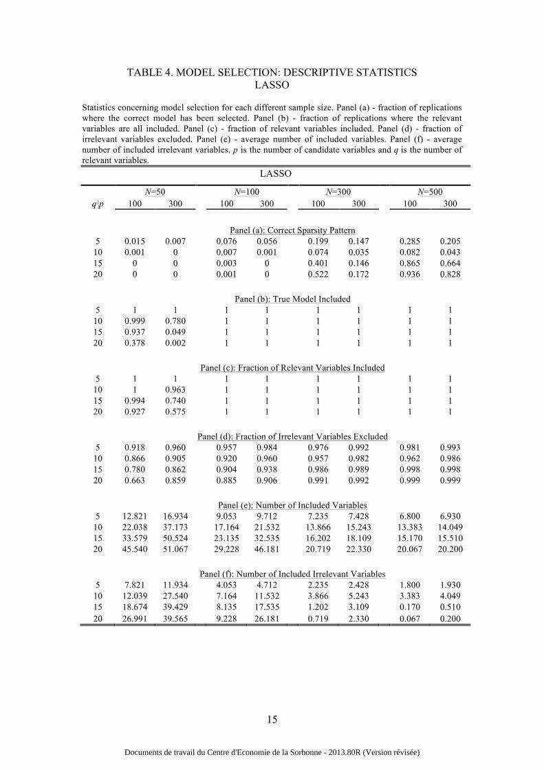
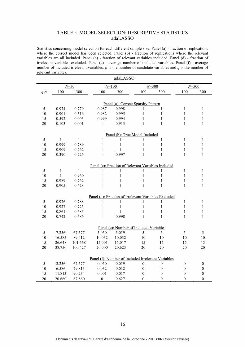
Tables 2 to 5 present variable selection results for each model selection

technique. Several related statistics are reported: Panel (a) presents the fraction of

replications where the correct model has been selected, i.e., all relevant variables

included and all irrelevant regressors excluded from the final model; Panel (b) shows

the fraction of replications where the relevant variables are all included; Panel (c)

presents the fraction of relevant variables included; Panel (d) shows the fraction of

irrelevant variables excluded; Panel (e) presents the average number of included

variables; Panel (f) shows the average number of included irrelevant variables. The

following comments point out the main results in Tables 2 to 5:

1. adaLASSO presents the best performance in finding the correct sparsity pattern in

most of the simulated scenarios. When N=300 and N=500, adaLASSO selects the

correct model every time.

2. When 𝑝 > 𝑁, LASSO and adaLASSO performance decreases dramatically as q

increases. In some extreme cases, adaLASSO includes more variables than

observations.

3. Autometrics (Conservative) shows better performance than Autometrics (Liberal).

As expected by definition of “target size”, the former includes less irrelevant

variables than the latter.

4. Autometrics (Conservative) shows best variable selection performance when

N=50.

5. Performance of all methodologies improves with the sample size (N) and gets

worse as the number of candidate variables (p) increases.

6. In most scenarios, performance of model selection methodologies gets worse as

the number of relevant variables (q) increases, especially when 𝑝 > 𝑁. However,

when 𝑝 < 𝑁, LASSO and adaLASSO show an improvement in their performance

for q=15 and q=20, explained by a feature of glmnet algorithm4.

Figure 1 shows the plot for Panel (a), (b), (c) and (c) of Tables 2 to 5: correct

4 The glmnet algorithm estimates different models for a decreasing sequence of λ’s. Values of λ are data driven and the maximum λ is the minimum value for which all coefficients estimates are zero. Different models are estimated for the entire sequence of λ and we use the BIC for the final model selection. The glmnet algorithm has also stopping criteria that can reduce the number of estimated models. When q=15 and q=20 the algorithm do not estimate models for the entire sequence of λ preventing the selection of over fitted models that minimize the BIC. For more details see glmnet vignette by Hastie, T. and Qian, J. (http://www.stanford.edu/~hastie/glmnet/glmnet_alpha.html).


12

sparsity pattern, true model included, fraction of relevant variables included and

fraction of irrelevant variables excluded. It is clear the superiority of adaLASSO to

others model selection methods, except the case of N=50, where the best method is

Autometrics (Conservative).

Finally, in order to compare predictive performance of the model selection

methods, Table 6 reports the root mean squared error for out-of-sample forecasts

(RMSFE) for Autometrics (Liberal and Conservative), LASSO, adaLASSO and

Oracle models. We consider a total of 100 out-of-sample observations. Main results of

Table 6 are summarized in the following comments:

1. As expected, all methodologies improve their performance as the sample size

increases, and the number of relevant (q) and candidate (p) variables decreases.

2. When 𝑝 < 𝑁 and q is small, adaLASSO and Autometrics (Conservative) present

similar performance to the Oracle model.

3. For q=15 or q=20, Autometrics (Conservative) presents lower RMSFE than

adaLASSO, especially when 𝑝 > 𝑁.


13

TABLE 2. MODEL SELECTION: DESCRIPTIVE STATISTICS Autometrics (Liberal)

Statistics concerning model selection for each different sample size. Panel (a) - fraction of replications where the correct model has been selected. Panel (b) - fraction of replications where the relevant variables are all included. Panel (c) - fraction of relevant variables included. Panel (d) - fraction of irrelevant variables excluded. Panel (e) - average number of included variables. Panel (f) - average number of included irrelevant variables. p is the number of candidate variables and q is the number of relevant variables.

Autometrics (Liberal)

N=50 N=100 N=300 N=500 q\p 100 300 100 300 100 300 100 300

Panel (a): Correct Sparsity Pattern

5 0.011 0 0.018 0 0.006 0 0.008 0 10 0.008 0 0.030 0 0.010 0 0.006 0 15 0.006 0 0.033 0 0.004 0 0.007 0 20 0.009 0 0.032 0 0.012 0 0.013 0

Panel (b): True Model Included

5 1 1 1 1 1 1 1 1 10 1 1 1 1 1 1 1 1 15 1 1 1 1 1 1 1 1 20 0.980 0.776 1 1 1 1 1 1

Panel (c): Fraction of Relevant Variables Included

5 1 1 1 1 1 1 1 1 10 1 1 1 1 1 1 1 1 15 1 1 1 1 1 1 1 1 20 0.994 0.922 1 1 1 1 1 1

Panel (d): Fraction of Irrelevant Variables Excluded

5 0.820 0.883 0.910 0.769 0.950 0.912 0.948 0.958 10 0.810 0.898 0.922 0.771 0.950 0.917 0.946 0.959 15 0.812 0.914 0.923 0.780 0.946 0.918 0.946 0.958 20 0.825 0.925 0.918 0.791 0.947 0.923 0.946 0.958

Panel (e): Number of Included Variables

5 22.056 39.532 13.544 73.173 9.728 31.041 9.979 17.337 10 27.103 39.577 17.026 76.438 14.542 34.139 14.870 21.981 15 30.990 39.526 21.575 77.559 19.551 38.326 19.602 26.905 20 33.882 39.419 26.595 78.381 24.227 41.518 24.306 31.846

Panel (f): Number of Included Irrelevant Variables

5 17.056 34.532 8.544 68.173 4.728 26.041 4.979 12.337 10 17.103 29.577 7.026 66.438 4.542 24.139 4.870 11.981 15 15.990 24.526 6.575 62.559 4.551 23.326 4.602 11.905 20 14.005 20.973 6.595 58.381 4.227 21.518 4.306 11.846


14

TABLE 3. MODEL SELECTION: DESCRIPTIVE STATISTICS Autometrics (Conservative)


Autometrics (Conservative)

N=50 N=100 N=300 N=500 q\p 100 300 100 300 100 300 100 300


5 0.425 0.091 0.447 0.115 0.357 0.201 0.341 0.075 10 0.398 0.054 0.523 0.206 0.391 0.209 0.365 0.085 15 0.369 0.029 0.513 0.182 0.378 0.163 0.384 0.068 20 0.368 0.023 0.529 0.144 0.430 0.147 0.413 0.073


5 1 1 1 1 1 1 1 1 10 1 1 1 1 1 1 1 1 15 1 1 1 1 1 1 1 1 20 0.911 0.839 1 1 1 1 1 1


5 1 1 1 1 1 1 1 1 10 1 1 1 1 1 1 1 1 15 1 1 1 1 1 1 1 1 20 0.966 0.946 1 1 1 1 1 1


5 0.986 0.966 0.987 0.976 0.988 0.991 0.988 0.989 10 0.984 0.959 0.990 0.988 0.988 0.991 0.988 0.989 15 0.983 0.953 0.990 0.987 0.987 0.989 0.988 0.989 20 0.982 0.955 0.990 0.985 0.988 0.989 0.988 0.989


5 6.355 14.977 6.213 12.158 6.169 7.797 6.144 8.293 10 11.401 21.911 10.883 13.476 11.088 12.753 11.037 13.125 15 16.452 28.299 15.878 18.707 16.083 18.190 16.056 18.148 20 20.767 31.550 20.816 24.338 20.937 23.148 20.978 23.142


5 1.355 9.977 1.213 7.158 1.169 2.797 1.144 3.293 10 1.401 11.911 0.883 3.476 1.088 2.753 1.037 3.125 15 1.452 13.299 0.878 3.707 1.083 3.190 1.056 3.148 20 1.452 12.628 0.816 4.338 0.937 3.148 0.978 3.142


15

TABLE 4. MODEL SELECTION: DESCRIPTIVE STATISTICS LASSO


LASSO

N=50 N=100 N=300 N=500 q\p 100 300 100 300 100 300 100 300


5 0.015 0.007 0.076 0.056 0.199 0.147 0.285 0.205 10 0.001 0 0.007 0.001 0.074 0.035 0.082 0.043 15 0 0 0.003 0 0.401 0.146 0.865 0.664 20 0 0 0.001 0 0.522 0.172 0.936 0.828


5 1 1 1 1 1 1 1 1 10 0.999 0.780 1 1 1 1 1 1 15 0.937 0.049 1 1 1 1 1 1 20 0.378 0.002 1 1 1 1 1 1


5 1 1 1 1 1 1 1 1 10 1 0.963 1 1 1 1 1 1 15 0.994 0.740 1 1 1 1 1 1 20 0.927 0.575 1 1 1 1 1 1


5 0.918 0.960 0.957 0.984 0.976 0.992 0.981 0.993 10 0.866 0.905 0.920 0.960 0.957 0.982 0.962 0.986 15 0.780 0.862 0.904 0.938 0.986 0.989 0.998 0.998 20 0.663 0.859 0.885 0.906 0.991 0.992 0.999 0.999


5 12.821 16.934 9.053 9.712 7.235 7.428 6.800 6.930 10 22.038 37.173 17.164 21.532 13.866 15.243 13.383 14.049 15 33.579 50.524 23.135 32.535 16.202 18.109 15.170 15.510 20 45.540 51.067 29.228 46.181 20.719 22.330 20.067 20.200


5 7.821 11.934 4.053 4.712 2.235 2.428 1.800 1.930 10 12.039 27.540 7.164 11.532 3.866 5.243 3.383 4.049 15 18.674 39.429 8.135 17.535 1.202 3.109 0.170 0.510 20 26.991 39.565 9.228 26.181 0.719 2.330 0.067 0.200


16

TABLE 5. MODEL SELECTION: DESCRIPTIVE STATISTICS adaLASSO


adaLASSO

N=50 N=100 N=300 N=500 q\p 100 300 100 300 100 300 100 300


5 0.974 0.779 0.987 0.998 1 1 1 1 10 0.901 0.316 0.982 0.995 1 1 1 1 15 0.592 0.003 0.999 0.994 1 1 1 1 20 0.103 0.001 1 0.913 1 1 1 1


5 1 1 1 1 1 1 1 1 10 0.999 0.789 1 1 1 1 1 1 15 0.909 0.262 1 1 1 1 1 1 20 0.390 0.226 1 0.997 1 1 1 1


5 1 1 1 1 1 1 1 1 10 1 0.960 1 1 1 1 1 1 15 0.989 0.762 1 1 1 1 1 1 20 0.905 0.628 1 1 1 1 1 1


5 0.976 0.788 1 1 1 1 1 1 10 0.927 0.725 1 1 1 1 1 1 15 0.861 0.683 1 1 1 1 1 1 20 0.742 0.686 1 0.998 1 1 1 1


5 7.256 67.577 5.050 5.019 5 5 5 5 10 16.585 89.412 10.032 10.032 10 10 10 10 15 26.648 101.668 15.001 15.017 15 15 15 15 20 38.750 100.427 20.000 20.623 20 20 20 20


5 2.256 62.577 0.050 0.019 0 0 0 0 10 6.586 79.813 0.032 0.032 0 0 0 0 15 11.813 90.234 0.001 0.017 0 0 0 0 20 20.660 87.860 0 0.627 0 0 0 0


17

FIGURE 1. MODEL SELECTION: COMPARISON

Panel (a), (b), (c) and (d) for Autometrics-Lib (red), Autometrics-Cons (yellow), LASSO (green) and adaLASSO (blue). p is the number of candidate variables, q is the number of relevant regressors and N is the sample size.


18

TABLE 6. FORECASTING: RMSFE

Root mean squared forecast error (RMSFE), for each model selection technique, for each different sample size. p is the number of candidate variables and q is the number of relevant variables.

N=50 N=100 N=300 N=500 q\p 100 300 100 300 100 300 100 300

RMSFE - Autometrics (Liberal) 5 0.172 0.163 0.126 0.181 0.105 0.123 0.103 0.108

10 0.186 0.170 0.127 0.186 0.106 0.122 0.104 0.108 15 0.203 0.177 0.130 0.190 0.107 0.123 0.104 0.109 20 0.285 1.002 0.136 0.195 0.107 0.123 0.105 0.110

RMSFE - Autometrics (Conservative) 5 0.116 0.145 0.108 0.126 0.102 0.105 0.101 0.103

10 0.125 0.165 0.110 0.119 0.103 0.106 0.102 0.103 15 0.137 0.178 0.113 0.125 0.104 0.107 0.102 0.104 20 0.427 0.737 0.116 0.132 0.105 0.108 0.103 0.105

RMSFE - LASSO 5 0.133 0.155 0.116 0.123 0.105 0.107 0.103 0.104

10 0.202 0.875 0.130 0.147 0.110 0.113 0.105 0.107 15 0.628 3.164 0.157 0.190 0.127 0.127 0.124 0.124 20 2.330 4.173 0.193 0.280 0.147 0.148 0.143 0.143

RMSFE – adaLASSO 5 0.123 0.216 0.104 0.106 0.102 0.102 0.101 0.101

10 0.219 0.927 0.112 0.117 0.105 0.105 0.103 0.103 15 0.609 2.892 0.137 0.137 0.125 0.125 0.122 0.122 20 2.219 3.858 0.161 0.175 0.145 0.146 0.141 0.140

RMSFE - Oracle 5 0.105 0.105 0.103 0.103 0.101 0.101 0.100 0.100

10 0.112 0.112 0.105 0.105 0.102 0.102 0.101 0.101 15 0.120 0.120 0.108 0.108 0.102 0.102 0.101 0.102 20 0.129 0.130 0.112 0.112 0.103 0.103 0.102 0.102


19

4. Application: Epidermal thickness in psoriatic patients

Psoriasis is a common chronic inflammatory skin disease, which the cause is not

entirely understood. Clinically, thickened epidermis is a major factor to measure

psoriasis severity.

With recent evolution of high-throughput technologies devoted to medical and

translational sciences, genomics databases are increasingly available, and the

development of high-dimensional statistical models becomes essential. In this

scenario, variable selection is a significant step, and some methodologies have already

been applied to genomics. Tian et al. (2012), Tian and Suárez-Fariñas (2013) and

Correa da Rosa et al. (2017) show applications of regularization algorithms for genes

selection in Psoriasis’ genomic data.

A set of histological measurements of epidermal thickness in a cohort of 609

psoriatic patients reported in Suárez-Fariñas et al. (2012)5 and a subcohort of 65

patients in Kim et al. (2015) were analysed and showed evidence of association

between gene expression levels and thick and thin plaque psoriasis phenotypes.

Despite the fact that the authors have identified psoriasis pathways with difference

between these two phenotypes, the quantitative epidermal thickness phenotype was

not used as an outcome. Additionally, enrichment analysis was only carried out for

psoriasis pathways.

In this section, we propose fill these gaps with the application of the two

described approaches. The epidermal thickness and microarray gene expressions from

54675 genes measured in a set of 70 patients analysed in Suárez-Fariñas et al. (2012)

will be used as dependent and regressors respectively. Due to the fact that Autometrics

does not support a General Unrestricted Model (GUM) with such a large number of

candidate variables, we used only a restricted set of 870 gene expressions6 as

regressors. The GUM is a linear model written in eq. (8).

5 We want to thank Mayte Suárez-Fariñas from the Icahn School of Medicine, Mount Sinai, New York, USA, for providing the data and all the help with the genetic language. 6 An initial set of 54675 candidate variables (microarray gene expressions at probesets) was reduced to a set of 870 genes by using moderated t-test statistics in linear mixed-effects models as implemented in limma package available in R/Bioconductor software.

𝑦! = 𝛽!𝑥!,!

!

!!!

+ 𝜀! , 𝑖 = 1,… ,𝑁

𝜀!~IN 0,𝜎! ,

(8)


20

where 𝑝 is 870 candidate variables.

We used 80% of the data for specification and estimation in-sample (56

patients) and the final 20% for out-of-sample forecasting (14 patients). We evaluated

1000 permutations on the data observations, creating 1000 different in-sample and

out-of-sample sets. The results presented next are the average statistics of the 1000

fitted models.

4.1. Results

We considered GUM in eq. (8) for specification and estimation by Autometrics,

LASSO and adaLASSO methods, and evaluate one-step ahead out-of-sample forecast.

Out-of-sample forecasting is evaluated in terms of two measures: root mean

squared forecast error (RMSFE) and an out-of-sample R2 statistics, defined as:

𝑅!!" = 1−𝑦! − 𝑦! !

𝑦! − 𝑦 !!∈!

, (9)

where Ο is the out-of-sample observations set and 𝑦 is the historical mean of the in-

sample set. Contrarily to usual R2, the out-of-sample R2 may be negative. If 𝑅!!" is

positive, then the selected model has lower average mean squared prediction error

than the historical average.

Table 7 presents results concerning estimation (in-sample) and forecasting (out-

of-sample) for model selection methods. With respect to variable selection and

estimation, Table 7 reports the average number of parameters and the average in-

sample R2, for selected final models. Concerning one-step ahead out-of-sample

forecasting, Table 7 presents the average root mean squared forecast error (RMSFE),

and average out-of-sample R2, defined in eq. (9). The following comments point out

the main results:

1. The out-of-sample forecasting performance of LASSO and adaLASSO models is

far superior to Autometrics (Liberal and Conservative) models.

2. The LASSO model presents the best predictive performance, i.e., the lowest

RMSFE and largest 𝑅!!".


21

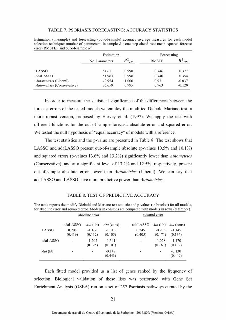
TABLE 7. PSORIASIS FORECASTING: ACCURACY STATISTICS

Estimation (in-sample) and forecasting (out-of-sample) accuracy average measures for each model selection technique: number of parameters; in-sample R2; one-step ahead root mean squared forecast error (RMSFE), and out-of-sample R2.

In order to measure the statistical significance of the differences between the

forecast errors of the tested models we employ the modified Diebold-Mariano test, a

more robust version, proposed by Harvey et al. (1997). We apply the test with

different functions for the out-of-sample forecast: absolute error and squared error.

We tested the null hypothesis of "equal accuracy" of models with a reference.

The test statistics and the p-value are presented in Table 8. The test shows that

LASSO and adaLASSO present out-of-sample absolute (p-values 10.5% and 10.1%)

and squared errors (p-values 13.6% and 13.2%) significantly lower than Autometrics

(Conservative), and at a significant level of 13.2% and 12.5%, respectively, present

out-of-sample absolute error lower than Autometrics (Liberal). We can say that

adaLASSO and LASSO have more predictive power than Autometrics.

TABLE 8. TEST OF PREDICTIVE ACCURACY

The table reports the modify Diebold and Mariano test statistic and p-values (in bracket) for all models, for absolute error and squared error. Models in columns are compared with models in rows (reference).

absolute error squared error

adaLASSO Aut (lib) Aut (cons)

adaLASSO Aut (lib) Aut (cons)

LASSO 0.208 -1.166 -1.316

0.245 -0.986 -1.145 (0.419) (0.132) (0.105) (0.405) (0.171) (0.136) adaLASSO - -1.202 -1.341

- -1.028 -1.170

(0.125) (0.101) (0.161) (0.132)

Aut (lib) - - -0.147 - - -0.130 (0.443) (0.449)

Each fitted model provided us a list of genes ranked by the frequency of

selection. Biological validation of these lists was performed with Gene Set

Enrichment Analysis (GSEA) run on a set of 257 Psoriasis pathways curated by the

Estimation Forecasting No. Parameters 𝑅!!" RMSFE 𝑅!!"

LASSO 54.611 0.998 0.746 0.377 adaLASSO 51.963 0.998 0.740 0.354 Autometrics (Liberal) 42.954 1.000 0.931 -0.037 Autometrics (Conservative) 36.659 0.995 0.963 -0.120


22

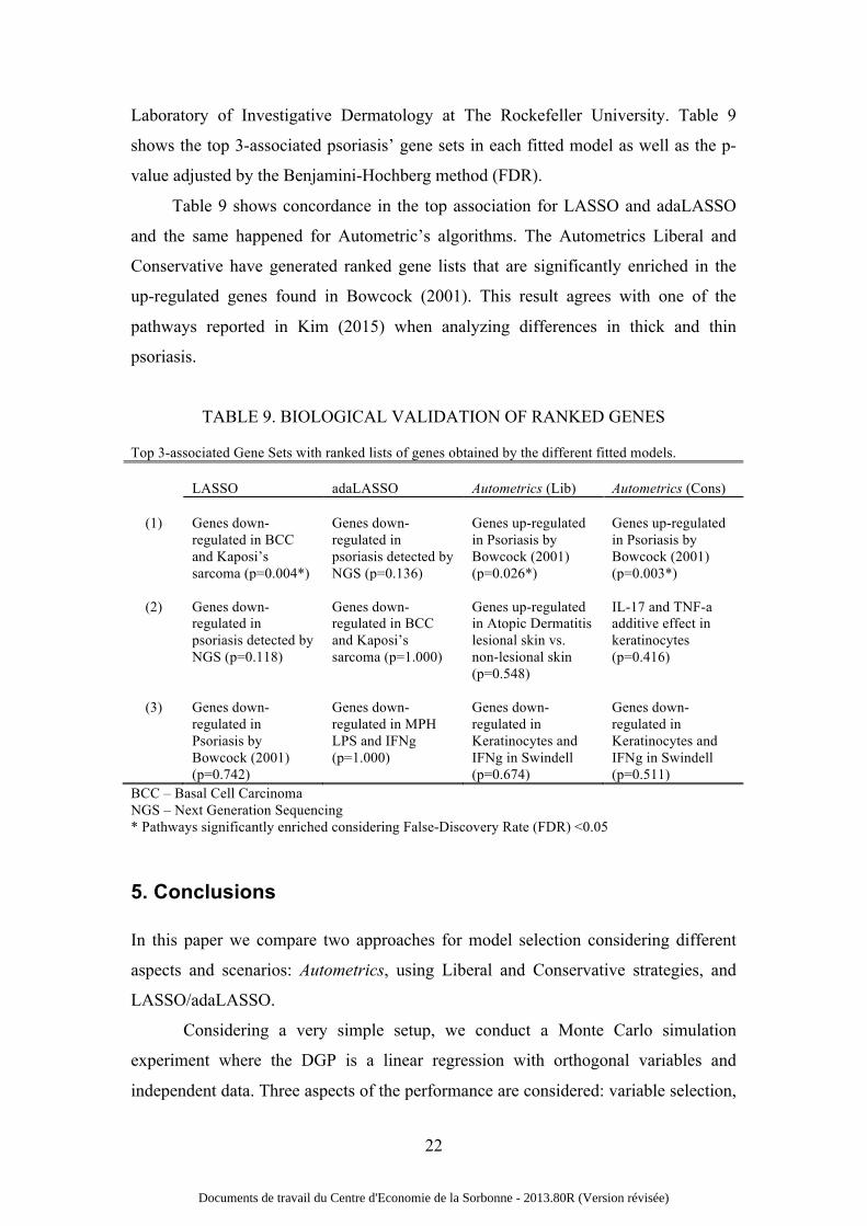
Laboratory of Investigative Dermatology at The Rockefeller University. Table 9

shows the top 3-associated psoriasis’ gene sets in each fitted model as well as the p-

value adjusted by the Benjamini-Hochberg method (FDR).

Table 9 shows concordance in the top association for LASSO and adaLASSO

and the same happened for Autometric’s algorithms. The Autometrics Liberal and

Conservative have generated ranked gene lists that are significantly enriched in the

up-regulated genes found in Bowcock (2001). This result agrees with one of the

pathways reported in Kim (2015) when analyzing differences in thick and thin

psoriasis.

TABLE 9. BIOLOGICAL VALIDATION OF RANKED GENES

Top 3-associated Gene Sets with ranked lists of genes obtained by the different fitted models. LASSO adaLASSO Autometrics (Lib) Autometrics (Cons)

(1) Genes down-regulated in BCC and Kaposi’s sarcoma (p=0.004*)

Genes down-regulated in psoriasis detected by NGS (p=0.136)

Genes up-regulated in Psoriasis by Bowcock (2001) (p=0.026*)

Genes up-regulated in Psoriasis by Bowcock (2001) (p=0.003*)

(2)

Genes down-regulated in psoriasis detected by NGS (p=0.118)

Genes down-regulated in BCC and Kaposi’s sarcoma (p=1.000)

Genes up-regulated in Atopic Dermatitis lesional skin vs. non-lesional skin (p=0.548)

IL-17 and TNF-a additive effect in keratinocytes (p=0.416)

(3)

Genes down-regulated in Psoriasis by Bowcock (2001) (p=0.742)

Genes down-regulated in MPH LPS and IFNg (p=1.000)

Genes down-regulated in Keratinocytes and IFNg in Swindell (p=0.674)

Genes down-regulated in Keratinocytes and IFNg in Swindell (p=0.511)

BCC – Basal Cell Carcinoma NGS – Next Generation Sequencing * Pathways significantly enriched considering False-Discovery Rate (FDR) <0.05

5. Conclusions

In this paper we compare two approaches for model selection considering different

aspects and scenarios: Autometrics, using Liberal and Conservative strategies, and

LASSO/adaLASSO.

Considering a very simple setup, we conduct a Monte Carlo simulation

experiment where the DGP is a linear regression with orthogonal variables and

independent data. Three aspects of the performance are considered: variable selection,


23

parameter estimation and predictive power, considering different sample sizes (N),

different number of relevant variables (q) and candidate variables (p). Simulation

results show that, as expected, all methods improve their performance as sample size

increases and the number of relevant and candidate variables decreases. Regarding

parameter estimation, Autometrics presents the lowest absolute average bias and

variance, as expected by the definition of OLS estimation when the correct model is

selected. LASSO and adaLASSO present similar results when N increases, however,

for small sample sizes, adaLASSO presents lower parameters average absolute bias

and variance.

Regarding variable selection, adaLASSO presents superior performance in most

of the simulated scenarios, except for N=50, where Autometrics (Conservative)

presents better results, especially if the number of relevant variables increases. When

N=300 and N=500, adaLASSO always selects the correct model whereas Autometrics

(Conservative) tends to include some irrelevant variables.

Concerning out-of-sample forecasting, for large values of q, even when

adaLASSO finds the correct sparsity pattern, Autometrics (Conservative) presents

better predictive performance. This is explained by the bias generated by the

penalization term in adaLASSO that has stronger effect in RMSFE as q increases. For

small values of q and 𝑝 < 𝑁, adaLASSO and Autometrics (Conservative) have similar

performance to the Oracle model.

A general conclusion is that, for a linear regression with orthogonal variables,

the adaLASSO has superior performance in model selection than LASSO and

Autometrics for almost every case (N=100, N=300 and N=500). However, for small

samples (N=50 in our experiment), it is preferable to use Autometrics (Conservative).

In the application to psoriasis forecasting, Autometrics cannot handle all the

genomic expressions as candidate variables in a feasible time. For that reason, the

initial set of 54675 variables was reduced to a set of 870 genes. Results showed that

LASSO and adaLASSO are much superior in predictive power than Autometrics.


24

Appendix

Cross-block algorithm proposed in Hendry and Krolzig (2004) in the case where the

number of candidate variables exceeds the number of observations in Autometrics:

1. dividing the set of variables into subsets (blocks), each of which contains less

than half of the observations,

2. applying Autometrics model selection to each combination of the blocks (GUMs).

The algorithm yields a terminal model for each GUM,

3. taking the union of the terminal models derived from each GUM, forming a new

single union model.

4. If the number of variables in this model is less than the number of observations,

model selection proceeds from this new union model (new unique GUM),

otherwise, restarts the cross-block algorithm with the new set of variables.

References

Bowcock AM, Shannon W, Du F, Duncan J, Cao K, Aftergut K, et al. (2001). Insights into psoriasis and other inflammatory diseases from large-scale gene expression studies. Human Molecular Genetics, 10(17), 1793–1805. Campos, J., D. F. Hendry, and H. M. Krolzig (2003). Consistent Model Selection by an Automatic Gets Approach. Oxford Bulletin of Economics and Statistics, 65, supplement, 803-819. Correa da Rosa J, Kim J, Tian S, Tomalin LE, Krueger JG, Suárez-Fariñas M. (2017). Shrinking the Psoriasis Assessment Gap: Early Gene-Expression Profiling Accurately Predicts Response to Long-Term Treatment. The Journal of Investigative Dermatology, 137(2), 305-312. Doornik, J. A. (2009). Autometrics. In J. L. Castle and N. Shephard (Eds.), The Methodology and Practice of Econometrics, pp. 88–122. Oxford University Press, Oxford. Efron, B., Hastie, T., Johnstone, I. and Tibshirani, R. (2004). Least angle regression, The Annals of Statistics, 32(2), 407-499. Fan, J. and Li, R. (2001). Variable selection via nonconcave penalized likelihood and its oracle properties. Journal of the American Statistical Association, 96, 1348–1360. Friedman, J. H., Hastie, T., Tibshirani, R. (2010). Regularized Paths for Generalized Linear Models via Coordinate Descent. Journal of Statistical Software, 33(1).


25

Harvey, D., Leybourne, S. and Newbold, P. (1997). Testing de equality of prediction mean squared errors. International Journal of Forcasting, 13, 281-291. Hendry, D. F., and Krolzig, H-M. (1999). Improving on ‘Data Mining Reconsidered’ by K. D. Hoover and S. J. Perez. Econometrics Journal, 2, 202-219. Hendry, D. F., and Krolzig, H.-M. (2004). Resolving three ‘intractable’ problems using a Gets approach. Unpublished paper, Economics Department, University of Oxford. Hendry, D.F. and B. Nielsen (2007), Econometric Modeling: A Likelihood Approach. Princeton University Press. Kim J, Nadella P, Kim DJ, Brodmerkel C, Correa da Rosa J, Krueger JG, Suárez-Fariñas M. (2015). Histological Stratification of Thick and Thin Plaque Psoriasis Explores Molecular Phenotypes with Clinical Implications. PLoS ONE, 10(7): e0132454. Krolzig, H-M. and Hendry, D.F. (2001). Computer automation of general-to-specific model selection procedures. Journal of Economic Dynamics and Control, 25, 831- 866. Medeiros, M. C. and Mendes, E. F. (2016). ℓ𝓁1-Regularization of High-dimensional Time-Series Models with Non-Gaussian and Heteroskedastic Innovations. Journal of Econometrics, 191, 255-271. Meinshausen, N. and Yu, B. (2009). Lasso-type recovery of sparse representations for high dimensional data. The Annals of Statistics, 37, 246–270. Perez-Amaral, T., Gallo, G. M. and White, H. (2003). A flexible tool for model building: the relevant transformation of the inputs network approach (RETINA). Oxford Bulletin of Economics and Statistics, Vol. 65, 821-838. Suárez-Fariñas, M., Li, K., Fuentes-Duculan, J., Hayden, K., Brodmerkel, C., Krueger, J. G. (2012). Expanding the psoriasis disease profile: interrogation of the skin and serum of patients with moderate-to-severe psoriasis. The Journal of Investigative Dermatology, 132(11), 2552-64. Tian, S., Krueger, J. G., Li, K., Jabbari, A., Brodmerkel, C., et al. (2012). Meta- Analysis Derived (MAD) Transcriptome of Psoriasis Defines the “Core” Pathogenesis of Disease. PLoS ONE 7(9): e44274. Tian, S., Suárez-Fariñas, M. (2013). Multi-TGDR: a regularization method for multi-class classification in microarray experiments. PLoS ONE 8(11): e78302. Tibshirani, R. (1996). Regression shrinkage and selection via the Lasso. Journal of the Royal Statistical Society. Series B (Methodological) 58(1), 267–288. Tibshirani, R. (2011). Regression shrinkage and selection via the lasso: a retrospective. JRSSB retrospective read paper, vol. 73, part 3, 273-282.


26

Wang, H., Li, G. and Tsai, C. (2007). Regression coefficient and autoregressive order shrinkage and selection via the lasso. Journal of the Royal Statistical Society: Series B (Statistical Methodology), 69(1), 63–78. White, H. (2006). Approximate nonlinear forecasting methods. In G. Elliott, C. W. J. Granger, and A. Timmermann (Eds.), Handbook of Economic Forecasting, Volume 1, pp. 459–512. Elsevier, Amsterdam. Zhang, Y., Li, R. and Tsai, C.-L. (2010). Regularization parameter selections via generalized information criterion. Journal of the American Statistical Association, 105, 312–323. Zhao, P. and Yu, B. (2006). On model consistency of lasso. Journal of Machine Learning Research, 7, 2541–2563. Zou, H. (2006). The adaptive lasso and its oracle properties. Journal of the American Statistical Association, 101, 1418–1429. Zou, H. and Hastie, T. (2005). Regularization and variable selection via the elastic net. Journal of Royal Statistical Society, Series B 67, 301–320. Zou, H., Hastie, T. and Tibshirani, R. (2007). On the degrees of freedom of the lasso. Annals of Statistics, 35, 2173–2192.
