Detecting and Forecasting Economic Regimes

in Automated Exchanges

Wolfgang Ketter⋆, John Collins†, Maria Gini†, Alok Gupta‡, and Paul Schrater†

⋆Dept. of Decision and Information Sciences, Rotterdam Sch. of Mgmt., Erasmus University†Dept. of Computer Science and Engineering, University of Minnesota

‡Dept. of Information and Decision Sciences, Carlson Sch. of Mgmt., University of Minnesota

wketter@rsm.nl, {jcollins,gini,schrater}@cs.umn.edu, agupta@csom.umn.edu

Abstract

We present basic building blocks of an agent that can use observable market conditions to characterizethe microeconomic conditions of the market and predict future market trends. The agent can use thisinformation to make both tactical decisions such as pricing and strategic decisions such as product mixand production planning. We develop methods that can learn dominant market conditions, such as over-supply or scarcity, from historical data using computational methods to construct price density functions.We discuss how this knowledge can be used, together with real-time observable information, to identifythe current dominant market condition and to forecast market changes over a planning horizon. Wevalidate our methods by presenting experimental results in a case study, the Trading Agent Competitionfor Supply Chain Management.

1 Introduction

Business organizations seeking advantage are increasingly looking to automated decision support systems.These systems have become increasingly sophisticated in recent years. Advanced decision support systemsare evolving into software agents that can act rationally on behalf of their users in a variety of applicationareas. Examples include procurement [27, 7], scheduling and resource management [12, 5], and personalinformation management [2, 21].

In this paper, we show how machine learning techniques can be used to support rational decision makingin a sales environment. We are particularly interested in environments that are constrained by capacity andmaterials availability. We demonstrate our approach in the context of an autonomous agent that is designedto compete in the Trading Agent Competition for Supply Chain Management (TAC SCM) [4].

Our method characterizes market conditions by distinguishable statistical patterns. We call these patternseconomic regimes. We show how such patterns can be learned from historical data and identified fromobservable data. We outline how to identify regimes and forecast regime transitions. This prediction, inturn, can be used to allocate resources to current and future sales in a way that maximizes resource value.While this type of prediction about the economic environment is commonly used at the macro economiclevel [24], such predictions are rarely done for a micro economic environment.

In addition to the supply-chain trading example, there are a number of other domains that could benefitfrom our approach. Examples include agents for automated trading in financial markets, such as the Penn-Lehman Automated Trading Project [13], auction-based contracting environments, such as MAGNET [6],and other auctions, such as auctions for IBM PCs [20] or PDA’s on eBay [9].

After a review of relevant literature, we describe in a general way the information needed to makestrategic and tactical sales decisions. We follow with a discussion of the concept of “economic regimes” andtheir representation using learned probability density functions. We then describe how this method is usedin an automated trading agent. For reader’s convenience, we present a summary of our notation in theAppendix.

1

2 Literature review

Predicting prices is an important part of the decision process of agents or human decision makers. Kephartet al. [14] explored several dynamic pricing algorithms for information goods, where shopbots look for thebest price, and pricebots adapt their prices to attract business. Wellman [32] analyzed and developed metricsfor price prediction algorithms in the TAC Classic game, similar to what we have done for TAC SCM.

Massey and Wu [22] show in their analysis that the ability of decision makers to correctly identify theonset of a new regime can mean the difference between success and failure. Furthermore they found strongevidence that individuals pay inordinate attention to the signal (price in our case), and neglect diagnosticity(regime probabilities) and transition probability (Markov matrix), the aspects of the system that generatesthe signal. Individuals who do not pay enough attention to regime identification and prediction have thetendency to over- or underreact to market conditions.

Ghose et al. [10] the authors empirically analyze the degree to which used products cannibalize newproduct sales for books on Amazon.com. In their study they show that product prices go through differentregimes over time. Marketing research methods have been developed to understand the conditions for growthin performance and the role that marketing actions can play to improve sales. For instance, in [26], an analysisis presented on how in mature economic markets strategic windows of change alternate with long periods ofstability.

Much work has focused on models for rational decision-making in autonomous agents. Ng and Russel [23]show that an agent’s decisions can be viewed as a set of linear constraints on the space of possible utility(reward) functions. However, the simple reward structure they used in their experiments will not scale towhat is needed to predict prices in more complex situations such as TAC SCM.

Chajewska, Koller, and Ormoneit [3] describe a method for predicting the future decisions of an agentbased on its past decisions. They learn the agent’s utility function by observing its behavior. Their approachis based on the assumption that the agent is a rational decision maker. According to decision theory, rationaldecision making amounts to maximization of the expected utility [31]. In TAC SCM, we cannot apply thesetechniques because the behaviors of individual agents are not directly observable.

Sales strategies used in previous TAC SCM competitions have attempted to model the probability ofreceiving an order for a given offer price, either by estimating the probability by linear interpolation fromthe minimum and maximum daily prices [25], or by estimating the relationship between offer price and orderprobability with a linear cumulative density function (CDF) [1], or by using a reverse CDF and factors suchas quantity and due date [15]. The Jackaroo team [33] applied a game theoretic approach to set offer prices,using a variation of the Cournot game for modeling the product market. The SouthamptonSCM [11] teamused fuzzy reasoning to set offer prices. Similar techniques have been used outside TAC SCM to predict offerprices in first price sealed bid reverse auctions for IBM PCs [20] or PDA’s on eBay [9].

In [17] the authors demonstrate a method for predicting future customer demand in the TAC SCM gameenvironment, and use the predicted future demand to inform agent behavior. Their approach is specific to theTAC SCM situation, since it depends on knowing the formula by which customer demand is computed. Notethat customer demand is only one of the factors for characterizing the multi-dimensional regime parameterspace.

All these methods fail to take into account market conditions that are not directly observable. They areessentially regression models, and do not represent qualitative differences in market conditions. Our method,in contrast, is able to detect and forecast a broader range of market conditions. Regression based approaches(including non-parametric variations) assume that the functional form of the relationship between dependentand independent variables has the same structure. An approach like ours that models variability and doesnot assume a functional relationship provides more flexibility and detects changes in relationship betweenprices and sales over time.

An analysis [16] of the TAC SCM 2004 competition shows that supply and demand (expressed as regimesin our method) are key factors in determining market prices, and that agents which were able to detect andexploit these conditions had an advantage.

2

3 Tactical and strategic decisions

We are primarily interested in competitive market environments that are constrained by resources and/orproduction capacity. In such an environment, a manager who wants to maximize the value of availableresources should be concerned about both strategic and tactical decisions. The basic strategic decision isto allocate available resources (financial, capacity, inventory, etc.) over some time horizon in a way that isexpected to return the maximum yield in the market. For example, in a market that has a strong seasonalvariation, one might want to build up an inventory of finished goods during the off season, when demand islow and prices are weak, in order to prepare for an expected period of strong demand and good prices. Forthe purpose of this paper, tactical decisions are concerned with setting prices to maximize profits, withinthe parameters set by the strategic decisions. So, for instance, if the forecast sales volume for the currentweek is 100,000 units, we would want to find the highest sales price that would move that volume.

Regime Identification Regime Prediction

Tactical

Decision Process Decision Process

Strategic

Figure 1: Process chart – Regime identification is a tool for tactical decision making and regime predictionis a tool for strategic decision making.

We believe that our technique of modeling the economic regimes in a market can be used to informboth the strategic and tactical decision processes. In Figure 1 we show a schematic way how to presentthis process. In our formulation, a regime is essentially a distribution of prices over sales volume. We usethis regime definition to characterize the market. By modeling an approximation of the probability of salegiven an asking price and combining with demand numbers, this leads directly to (nearly) optimal pricingdecisions.

In order to use our technique to inform the strategic decision process, we need to be able to forecastregime shifts in the market. If our forecast shows an upcoming period of low demand and weak prices, wemay want to sell more aggressively in the short term, and we may want to limit procurement and productionto prevent driving an oversupply into the market. On the other hand, if our forecast shows an upcomingperiod of high demand and strong prices, we may want to increase procurement and production, and raiseshort-term prices, in order to be well-positioned for the future.

4 Economic regimes

Market conditions change over time, and this should affect the strategy used by an agent in procurement,production planning, and product pricing. Economic theory suggests that economic environments exhibit 3dominant market patterns: scarcity, balanced, and oversupply. We define a scarcity condition if there is morecustomer demand than product supply in the market, a balanced condition if demand is approximately equalto supply, and an oversupply condition if there is less customer demand than product supply in the market.When there is scarcity, prices are higher, so the agent should price more aggressively. In balanced situations,prices are lower and have more spread, so the agent has a range of options for maximizing expected profit.In oversupply situations prices are lower. The agent should primarily control costs, and therefore either dopricing based on costs, or wait for better market conditions.

3

Figure 2 shows typical curves for the probability of receiving an order for a given offer price. The slopeof the curve and its position changes over time. According to economic theory, high prices and a steep slopecorrespond to a situation of scarcity, where price elasticity is small, while a less steep slope corresponds toa balanced market where the range of prices is larger.

We believe that even though the market is constantly changing, there are some underlying dominantpatterns which characterize the aforementioned market conditions. We define a specific mode a market canbe in as a regime. A way of solving the decision problem an agent is faced with is to characterize thoseregimes and to apply specific decision making methods to each regime. This requires an agent to havemethods for figuring out what is the current regime and for predicting which future regimes will be in itsplanning horizon.

Scarcity:

1

Price

Prob

abili

ty o

f O

rder

Balanced:

1

Prob

abili

ty o

f O

rder

Priceoversupply:

1

Price

Prob

abili

ty o

f O

rder

0 0.2 0.4 0.6 0.8 1 1.20

0.1

0.2

0.3

0.4

0.5

0.6

0.7

0.8

0.9

1O

rder

Pro

babi

lity

Normalized Price

1−2021−4041−6061−8081−100101−120121−140141−160161−180181−200201−220

Figure 2: The reverse cumulative density function represents probability of order. Typical order proba-bility curves during scarcity (left top), balanced (left middle) and oversupply (left bottom) regimes andexperimental order probability curves (right).The curves shown on the right are from TAC SCM data and are measured at different days from the startof the game.

4.1 Analysis of historical data to characterize market regimes

The first phase in our approach is to identify and characterize market regimes by analyzing data from pastsales. The assumption we make is that enough historical data are available for the analysis and that historical

4

data are sufficiently representative of possible market conditions. Information observable in real-time in themarket is then used to identify the current regime and to forecast regime transitions.

Since product prices are likely to have different ranges for different products, we normalize them. Wecall np the normalized price and define it as follows:

np =ProductPrice

NominalProductCost(1)

=ProductPrice

AssemblyCost +∑numParts

j=1 NominalPartCostj(2)

where NominalPartCostj is the nominal cost of the j-th part, numParts is the number of parts needed tomake the product, and AssemblyCost is the cost of manufacturing the product. An advantage of usingnormalized prices is that we can easily compare price patterns across different products.

Historical data are used to estimate the price density, p(np), and to characterize regimes. We startby estimating the price density function by fitting a Gaussian mixture model (GMM) [30] to historicalnormalized price, np, data. We use a GMM since it is able to approximate arbitrary density functions.Another advantage is that the GMM is a semi-parametric approach which allows for fast computing anduses less memory than other approaches.

In this paper, we present results using a GMM with fixed means, µi, and fixed variances, σi, since wewant one set of Gaussians to work for all games off-line and online. We use the Expectation-Maximization(EM) Algorithm [8] to determine the prior probability, P (ci), of the Gaussians components of the GMM.The means, µi, are uniformly distributed and the variances, σ2

i , tile the space. Specifically variances werechosen so that adjacent Gaussians are two standard deviations apart.

The density of the normalized price can be written as:

p(np) =

N∑

i=1

p(np|ci) P (ci) (3)

where p(np|ci) is the i-th Gaussian from the GMM, i.e.,

p(np|ci) = p(np|µi, σi) =1

σi

√2π

e

[

−(np−µi)2

2×σ2i

]

(4)

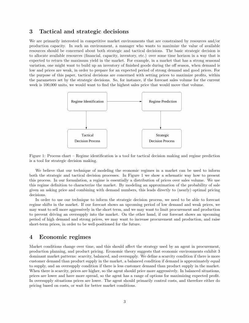
where µi is the mean and σi is the standard deviation of the i-th Gaussian from the GMM. An example ofa GMM is shown in Figure 3. While the choice of N , the number of Gaussians’, in a GMM is arbitrary,the choice should reflect a balance between accuracy and computational overhead. By accuracy we meanpredicted accuracy, which is not the same as fit accuracy. Creating a model with a very good fit to theobserved data does not usually translate well into predictions. If the model has too many degrees of freedomthe likelihood of overfitting the data is great. We chose N = 16 and N = 25 to show the effect of modelflexibility on results for several prediction measures and illustrate their tradeoffs.

Using Bayes’ rule we determine the posterior probability:

P (ci|np) =p(np|ci) P (ci)

∑N

i=1 p(np|ci) P (ci)∀i = 1, · · · , N (5)

We then define the posterior probabilities of all Gaussians’ given a normalized price, np, as the followingN-dimensional vector:

~η(np) = [P (c1|np), P (c2|np), . . . , P (cN |np)]. (6)

For each normalized price npj we compute the vector of the posterior normalized price probabilities, ~η(npj),which is ~η evaluated at each observed normalized price npj .

The intuitive idea of a regime as recurrent economic condition is captured by discovering price distri-butions that recur across days. We define regimes by clustering price distributions across days using thek-means algorithm with a similarity measure on both probability vectors ~η(npj) and normalized prices np.

5

0 0.2 0.4 0.6 0.8 1 1.20

5

x 104

Pro

duct

Qua

ntity

Normalized Price (np)0 0.2 0.4 0.6 0.8 1 1.2

0

2

p(np

)

0 0.2 0.4 0.6 0.8 1 1.20

2

Product Quantityp(np)

Figure 3: The price density density function, p(np), (right y-axis) estimated by the Gaussian mixture modelwith 16 components fits well the historical normalized price data (left y-axis represents product quantity)for a sample market. Data are from 18 games from semi-finals and finals of TAC SCM 2005.

The clusters found by this method correspond to frequently occurring price distributions with support oncontiguous range of np.1

The center of each cluster (ignoring the last component which contains the rescaled price information) isa probability vector that corresponds to regime r = Rk for k = 1, · · · , M , where M is the number of regimes.Collecting these vectors into a matrix yields the conditional probability matrix P(c|r). The matrix has N

rows, one for each component of the GMM, and M columns, one for each regime.In Figure 4 we distinguish five regimes, which we can call extreme oversupply (R1), oversupply (R2),

balanced (R3), scarcity (R4), and extreme scarcity (R5). We decided to use five regimes instead of the threebasic regimes which are suggested by economic theory because in this way we are able to isolate outlierregimes, such as extreme oversupply and extreme scarcity, in a market. Regimes R1 and R2 represent asituation where there is a glut in the market, i.e. an oversupply situation, which depresses prices. RegimesR3 represents a balanced market situation, where most of the demand is satisfied. In regime R3 the agenthas a range of options of price vs sales volume. Regimes R4 and R5 represent a situation where there isscarcity of products in the market, which increases prices. In this case the agent should price as close aspossible to the estimated maximum price a customer is willing to pay.

For the TAC SCM domain, the number of regimes was selected a priori, after examining the data andlooking at economic analyses of market situations. In our experiments we found out that the number ofregimes chosen does not significantly affect the results regarding price trend predictions. The computationof the GMM and k-means clustering were tried with different initial conditions, but consistently convergedto the same results.

We marginalize the product of the density of the normalized price, np, given the i-th Gaussian of theGMM, p(np|ci), and the conditional probability clustering matrix, P (ci|Rk), over all Gaussians ci. We obtain

1We have found that sometimes data points corresponding to specific regimes are close in probability space, but not in

price space. Specifically it can happen that one regime dominates the extreme low and the extreme high price range, with

different regimes in between. This regime is more difficult to interpret in terms of market concepts like oversupply or scarcity.

To circumvent this problem we perform clustering in an augmented space formed by appending a rescaled version of np to the

probability vector. Specifically, the mean of np is subtracted and np is scaled so that its standard deviation matches the largest

standard deviation of the probability vectors.

6

0 0.25 0.5 0.75 1 1.250

0.1

0.2

0.3

0.4

0.5

0.6

0.7

0.8

0.9

1

Normalized Price

Reg

ime

Pro

babi

lity

P(R

k|np)

EOOBSES

Figure 4: An example of learned regime probabilities , P (Rk|np), over normalized price np, for a samplemarket in TAC SCM after training.

the density of the normalized price np dependent on the regime Rk:

p(np|Rk) =

N∑

i=1

p(np|ci) P (ci|Rk). (7)

The probability of regime Rk dependent on the normalized price np can be computed using Bayes rule as:

P (Rk|np) =p(np|Rk) P (Rk)

∑M

k=1 p(np|Rk) P (Rk)∀k = 1, · · · , M. (8)

where M is the number of regimes. The prior probabilities, P (Rk), of the different regimes are determinedby a counting process over past data. Figure 4 depicts the regime probabilities for a sample market in TACSCM. Each regime is clearly dominant over a range of normalized prices.

The intuition behind regimes is that prices communicate information about future expectations of themarket. However, absolute prices do not mean much because the same price point can be achieved in astatic mode (i.e., when prices don’t change), when prices are increasing, or when prices are decreasing.In the construction of a regime the variation in prices (the nature, variance, and the neighborhood) areconsidered thereby providing a better assessment of market conditions.

We model regime prediction as a Markov process. The last step is the computation of the Markovtransition matrix to be used by the agent for regime prediction. We construct the Markov transition matrix,Tpredict(rt+1|rt) by a counting process over past data. This matrix represents the posterior probability oftransitioning at time step t + 1 to regime rt+1 given the current regime rt at time step t.

4.2 Identification of current regime

Previous sales data are used to learn the characterization of different market regimes. In real-time an agentcan then use this regime information to identify the dominant regime. This can be done by calculating (orestimating) the normalized prices for the current time step, t.

Since complete current price information might not be available, we indicate the estimated normalizedprice at time t by npt. Depending on the application domain, the price estimate can be accurate, or can bean approximation.

7

The agent selects the regime which has the highest probability, i.e.

argmax1≤k≤M

~P (Rk|npt).

4.3 Regime prediction

The prediction of regime probabilities is based on two distinct operations:

1. a correction (recursive Bayesian update) of the posterior probabilities for the regimes based on thehistory of measurements of the estimated median normalized prices obtained since the time of the lastregime change until the current time step.

2. prediction of the posterior distribution of regimes n time steps into the future, done recursively.

If the data for the current time-step is unavailable then we need to include after the correction operationa one time-step prediction to the current time before we do a prediction of future regime. The agent can usethis forecast of regime transitions to drive its strategic decision process.

5 A case study: TAC SCM

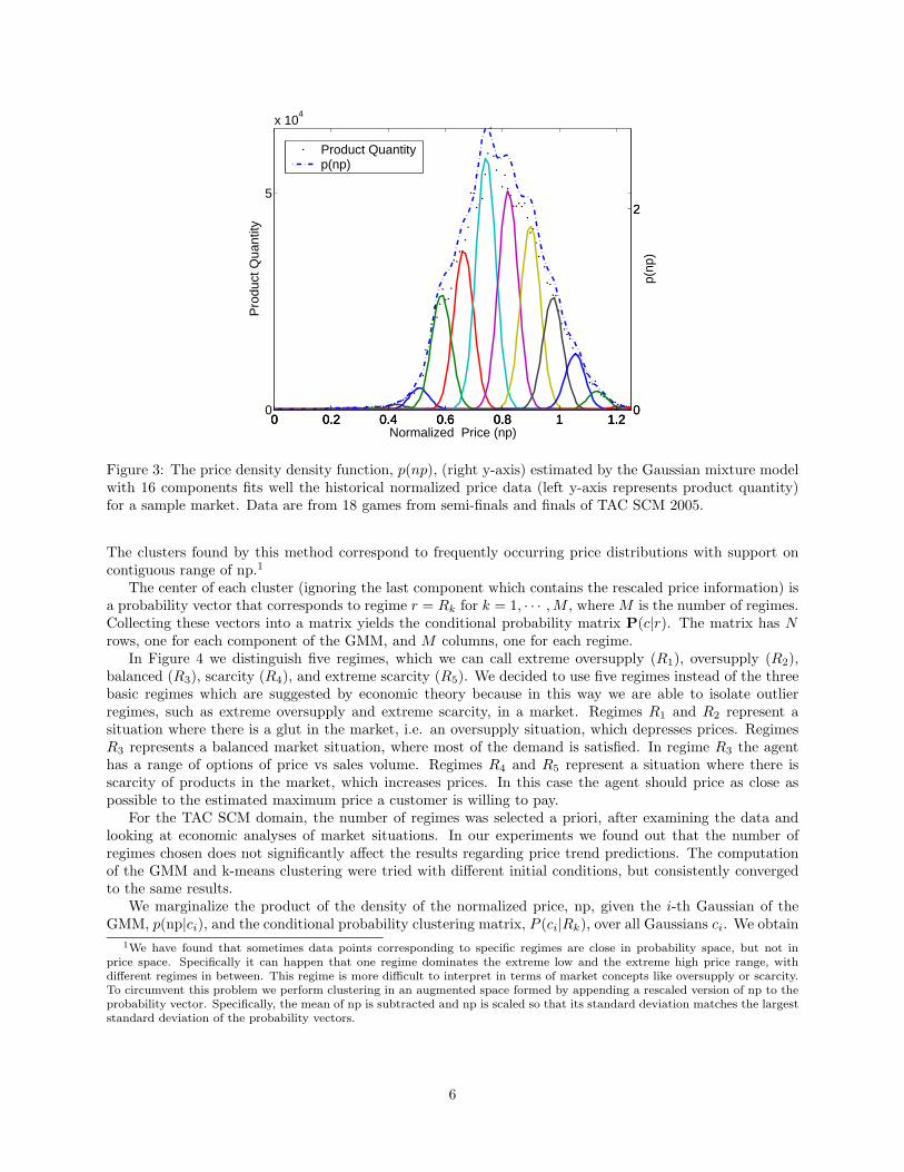
The Trading Agent Competition for Supply Chain Management [4] (TAC SCM) is a market simulation inwhich six autonomous agents compete to maximize profits in a computer-assembly scenario. The simulationtakes place over 220 virtual days, each lasting fifteen seconds of real time. Agents earn money by sellingcomputers they assemble out of parts they purchase from suppliers. Each agent has a limited-capacityassembly facility, and must pay for warehousing its inventory. In addition, each agent has a bank accountwith an initial balance of zero. The agent with the highest bank balance at the end of the game wins.

Offers

RFQs

Orders

Shipments

MinneTAC

TACTex

PSUTac

RedAgent

DeepMaize

Mertacor

RFQs

Offers

Orders

Shipments

Pintel

IMD

Basus

Macrostar

Mec

Queenmax

Watergate

Mintor

Suppliers Agents Customers

Figure 5: Schematic overview of a typical TAC SCM game scenario.

To obtain parts, an agent must send a request for quotes (RFQ) to an appropriate supplier. Each RFQspecifies a component type, a quantity, and a due date. The next day, the agent will receive a responseto each request. Suppliers respond by evaluating each RFQ to determine how many components they candeliver on the requested due date, considering the outstanding orders they have committed to and at what

8

price. If the supplier can produce the desired quantity on time, it responds with an offer that contains theprice of the supplies. If not, the supplier responds with two offers: (1) an earliest complete offer with arevised due date and a price. This revised due date is the first day in which the supplier believes it will beable to provide the entire quantity requested; and (2) a partial offer with a revised quantity and a price withthe requested due date. The agent can accept either of these alternative offers, or reject both. Suppliersmay deliver late, due to uncertainty in their production capacities. Suppliers discount part prices accordingto the ratio of supply to demand.

Every day each agent receives a set of RFQs from potential customers. Each customer RFQ specifiesthe type of computers requested, along with quantity, due date, reserve price, and penalty for late delivery.Each agent may choose to bid on some or all of the day’s RFQs. Customers accept the lowest bid that is ator below the reserve price, and notify the winning agent. The agent must ship customer orders on time, orpay the penalty for each day an order is late. If a product is not shipped within five days of the due datethe order is canceled, the agent receives no payment, and no further penalties accrue.

An agent can produce 16 different types of computers, that are categorized into three different marketsegments (low, medium, and high). Demand in each market segment varies randomly during the game.Other variables, such as storage costs and interest rates also vary between games.

The other agents playing in the same game affect significantly the market, since they all compete for thesame parts and customers. This complicates the operational and strategic decisions an agent has to makeevery day during the game, which include how many parts to buy, when to get the parts delivered, how toschedule its factory production, what types of computers to build, when to sell them, and at what price.

5.1 Experimental setup

For our experiments, we used data from a set of 24 games (18 for training2 and 6 for testing3) played duringthe semi-finals and finals of TAC SCM 2005. The mix of players changed from game to game, the totalnumber of players was 12 in the semi-finals and 6 in the finals.

Since supply and demand in TAC SCM change in each of the market segments (low, medium, and high)independently of the other segments, our method is applied to each individual market segment.

Each type of computer has a nominal cost, which is the sum of the nominal cost of each of the partsneeded to build it. In TAC SCM the cost of the facility is sunk, and there is no per-unit assembly cost. Wenormalize the prices across the different computer types in each market segment.

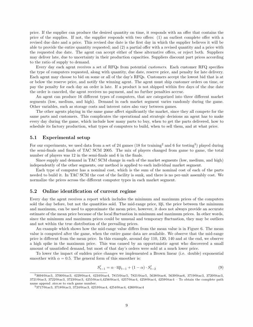
5.2 Online identification of current regime

Every day the agent receives a report which includes the minimum and maximum prices of the computerssold the day before, but not the quantities sold. The mid-range price, np, the price between the minimumand maximum, can be used to approximate the mean price, however, it does not always provide an accurateestimate of the mean price because of the local fluctuation in minimum and maximum prices. In other words,since the minimum and maximum prices could be unusual and temporary fluctuation, they may be outliersand not within the true distribution of the prevailing prices.

An example which shows how the mid-range value differs from the mean value is in Figure 6. The meanvalue is computed after the game, when the entire game data are available. We observe that the mid-rangeprice is different from the mean price. In this example, around day 110, 120, 140 and at the end, we observea high spike in the maximum price. This was caused by an opportunistic agent who discovered a smallamount of unsatisfied demand, but most of that day’s orders were sold at a much lower price.

To lower the impact of sudden price changes we implemented a Brown linear (i.e. double) exponentialsmoother with α = 0.5. The general form of this smoother is:

S′t−1 = α · npt−1 + (1 − α) · S′

t−2 (9)

23694@tac3, 3700@tac3, 4229@tac4, 4234@tac4, 7815@tac5, 7821@tac5, 5638@tac6, 5639@tac6, 3719@tac3, 3720@tac3,

3721@tac3, 3722@tac3, 3723@tac3, 4255@tac4,4256@tac4, 4257@tac4, 4258@tac4, 4259@tac4 – To obtain the complete path

name append .sics.se to each game number.33717@tac3, 3718@tac3, 3724@tac3, 4253@tac4, 4254@tac4, 4260@tac4

9

S′′t−1 = α · S′

t−1 + (1 − α) · S′′t−2 (10)

npt−1 = 2 · S′t−1 − S′′

t−1 (11)

Since we only have the minimum and maximum prices from the previous day available and not the realmean, we decided to model npt−1 as follows:

npt−1 =npmin

t−1 + npmaxt−1

2(12)

This results in a better approximation of the real mean price than smoothing only the mid-range price fromthe previous day. Figure 6 shows that the smoothed mid-range price, np, is closer to the mean price.

0 20 40 60 80 100 120 140 160 180 200 2200

0.2

0.4

0.6

0.8

1

1.2

Time in Days

Nor

mal

ized

Pric

e

Maximum PriceMean PriceMid−Range PriceSmoothed PriceMinimum Price

Figure 6: Minimum, maximum, mean, mid-range, and smoothed mid-range daily normalized prices of com-puters sold, as reported during the game every day for the medium market segment in the 3721@tac3, oneof the final games. The mean price is computed after the game using the game data, which include completeinformation on all the transactions.

During the game, the agent estimates on day t the current regime by calculating the smoothed mid-range normalized price npt−1 for the previous day (recall that the agent every day receives the prices for the

previous day) and by selecting the regime which has the highest probability, i.e. argmax1≤k≤M~P (Rk|npt−1).

The smoothed mid-range price can be used to identify the corresponding regime online, as shown inFigure 7 (right). The data are from game 3721@tac3, which was not in the training set of games used todevelop the regime definitions. The top left, middle left, and bottom left parts of Figure 7 show respectivelythe probability of receiving an order in an extreme scarcity, balanced and in an extreme over-supply situationfor different prices. Scarcity typically occurs early in the game and at other times when supply is low. Theseprobabilities are computed from past game data for each regime.

Figure 8 shows the relative probabilities of each regime over the course of a game. The graph showsthat different regimes are dominant at different points in the game, and that there are brief intervals duringwhich two regimes are almost equally likely. An agent could use this information to decide which strategy,or mixture of strategies, to follow.

A measure of the confidence in the regime identification is the entropy of the set S of probabilities of theregimes given the normalized mid-range price from the daily price reports npday, where

S = {P (R1|npday), · · · , P (RM |npday)} (13)

10

Extreme Scarcity:

0 0.2 0.4 0.6 0.8 1 1.20

0.1

0.2

0.3

0.4

0.5

0.6

0.7

0.8

0.9

1

Normalized Price (np)

Ord

er P

roba

bilit

y

Balanced:

0 0.2 0.4 0.6 0.8 1 1.20

0.1

0.2

0.3

0.4

0.5

0.6

0.7

0.8

0.9

1

Normalized Price (np)

Ord

er P

roba

bilit

y

Extreme Oversupply:

0 0.2 0.4 0.6 0.8 1 1.20

0.1

0.2

0.3

0.4

0.5

0.6

0.7

0.8

0.9

1

Normalized Price (np)

Ord

er P

roba

bilit

y

0 20 40 60 80 100 120 140 160 180 200 220

EO

O

B

S

ES

Time in Days

Reg

imes

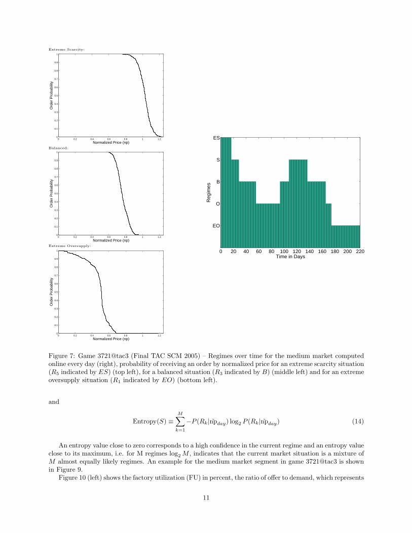
Figure 7: Game 3721@tac3 (Final TAC SCM 2005) – Regimes over time for the medium market computedonline every day (right), probability of receiving an order by normalized price for an extreme scarcity situation(R5 indicated by ES) (top left), for a balanced situation (R3 indicated by B) (middle left) and for an extremeoversupply situation (R1 indicated by EO) (bottom left).

and

Entropy(S) ≡M∑

k=1

−P (Rk|npday) log2 P (Rk|npday) (14)

An entropy value close to zero corresponds to a high confidence in the current regime and an entropy valueclose to its maximum, i.e. for M regimes log2 M , indicates that the current market situation is a mixture ofM almost equally likely regimes. An example for the medium market segment in game 3721@tac3 is shownin Figure 9.

Figure 10 (left) shows the factory utilization (FU) in percent, the ratio of offer to demand, which represents

11

0 20 40 60 80 100 120 140 160 180 200 2200

0.2

0.4

0.6

0.8

1

Time in Days

P(R

|np)

EOOBSES

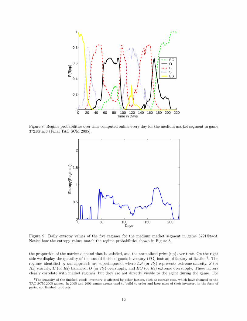
Figure 8: Regime probabilities over time computed online every day for the medium market segment in game3721@tac3 (Final TAC SCM 2005).

0 50 100 150 2000

0.5

1

1.5

2

Days

Ent

ropy

(Reg

imes

)

Figure 9: Daily entropy values of the five regimes for the medium market segment in game 3721@tac3.Notice how the entropy values match the regime probabilities shown in Figure 8.

the proportion of the market demand that is satisfied, and the normalized price (np) over time. On the rightside we display the quantity of the unsold finished goods inventory (FG) instead of factory utilization4. Theregimes identified by our approach are superimposed, where ES (or R5) represents extreme scarcity, S (orR4) scarcity, B (or R3) balanced, O (or R2) oversupply, and EO (or R1) extreme oversupply. These factorsclearly correlate with market regimes, but they are not directly visible to the agent during the game. For

4The quantity of the finished goods inventory is affected by other factors, such as storage cost, which have changed in the

TAC SCM 2005 games. In 2005 and 2006 games agents tend to build to order and keep most of their inventory in the form of

parts, not finished products.

12

0 50 100 150 2000

50

100F

acto

ry U

tiliz

atio

n (F

U)

in %

Day0 50 100 150 200

0

1

Nor

mal

ized

Pric

e (n

p)

0 50 100 150 2000

1

FUnpOffer/Demand

ES S S B B B O O EO

Regime Change

0 50 100 150 2000

1000

2000

Fin

ishe

d G

oods

Inve

ntor

y (F

G)

Day0 50 100 150 200

0

0.5

1

Nor

mal

ized

Pric

e (n

p)

0 50 100 150 2000

0.5

1

FGnpOffer/Demand

ES S S B B B O O EO

Regime

Change

Figure 10: Game 3721@tac3 (Final TAC SCM 2005) – Relationships between regimes and normalized pricesin the medium market. On the left axis, we show in the left figure the daily factory utilization and in theright figure the available finished goods inventory of all agents. In both figures we display on the left axis aswell the ratio of offer to demand (which ranges from 0 to 5.38), which is scaled to fit between the minimumand maximum values of the left axis. On the right axis we show the normalized prices. The dominantregimes are labeled along the bottom.

example, the figure shows that when the offer to demand ratio is high (i.e. oversupply) prices are low andvice versa. We can observe that the ratio of offer to demand changes significantly during the game. Forinstance, on day 111 the ratio of offer to demand is 1.95 and prices are high. On day 208 the ratio of offerto demand is much higher, 5.38, and prices are lower. We can also observe that prices tend to lag changesin ratio of offer to demand.

5.3 Predicting regime transitions

For TAC SCM, we model the prediction of future regimes as a Markov process. We construct a Markovtransition matrix, Tpredict(rt+1|rt) off-line by a counting process over past games. This matrix representsthe posterior probability of transitioning in day t + 1 to regime rt+1 given the current regime in day t, rt.

The prediction of regime probabilities is based on two distinct operations:

1. a correction (recursive Bayesian update) of the posterior probabilities for the regimes based on thehistory of measurements of the smoothed mid-range normalized price np obtained since the time ofthe last regime change, t0, until the previous day, t− 1. We use ~P (rt−1|{npt0

, . . . , npt−1}), to indicatea vector of the posterior probabilities of all the regimes on day t − 1.

2. a prediction of regime posterior probabilities for the current day, t. The prediction of the posteriordistribution of regimes n days into the future, ~P (rt+n|{npt0

, . . . , npt−1}), is done recursively as follows:

~P (rt+n|{npt0, . . . , npt−1})

=∑

rt+n

· · ·∑

rt−1

{

~P (rt−1|{npt0, . . . , npt−1}) ·

n∏

j=0

Tpredict(rt+j |rt+j−1)

}

(15)

Examples of regime predictions for game 3721@tac3 for the medium market segment are shown in Fig-ure 11 and Figure 12. The figures show the real regimes measured after the game from the game data andthe predictions made by our method during the game. As it can be seen in the figures, the match betweenpredictions and real data is very good.

Figure 11 shows a predicted change from from an oversupply situation to a balanced situation. Thismeans that the agent should sell less today and build up more inventory for future days when prices will be

13

80 85 90 95 100

EO

O

B

S

ESO

ff−lin

e

80 85 90 95 100

EO

O

B

S

ES

Time in Days

Pre

dict

ion

Figure 11: Regime predictions for game3721@tac3 starting on day 80 for 20 days into thefuture for the medium market segment. Data areshown as computed after the game using the com-plete set of data, and as predicted by our methodduring the game.

110 115 120 125 130 135 140

EO

O

B

S

ES

Off−

line

110 115 120 125 130 135 140

EO

O

B

S

ES

Time in Days

Pre

dict

ion

Figure 12: Regime predictions for game3721@tac3 starting on day 110 for 30 days intothe future for the medium market segment.

higher. On the other hand we see in Figure 12 a predicted change from the scarcity to the balanced regime.In this case the agent should try to sell more aggressively the current day, since prices will be decreasing inthe next days.

6 Performance of regime identification and prediction

Our method is useful to the extent that it characterizes and predicts real qualities of the market. Thereare many hidden variables in a competitive market, such as the inventory positions and procurement ar-rangements of the competitors. Our method uses observable historical and current data to guide tacticaland strategic decision processes. In this section we evaluate the practical value of regime identification andprediction.

6.1 Relationship between identified regime and market variables

We expect identified regimes to qualitatively represent the status of the important hidden market factors.A correlation analysis of market parameters of the training set is shown in Figure 13. The p-values forthe correlation analysis are all less than 0.01. Regime EO (extreme oversupply) correlates positively withquantity of finished goods inventory, negatively with percent of factory utilization, positively with the ratio ofoffer to demand, and negatively with normalized price. On the other hand, in Regime ES (extreme scarcity)we observe a negative correlation with the amount of unsold finished goods inventory, with the percent offactory utilization, and the ratio of offer to demand, and positively with normalized price.

An advantage of using 5 regimes instead of 3 regimes is that we gain two degrees of freedom for betterdecision making, by isolating the outliers in the market. For example, regime EO (extreme oversupply) isdifferent from Regime O (oversupply) since it presents a potential price war situation. Another differencebetween regime EO and regime O is that regime EO is universally unprofitable and that regime O ismarginally profitable for most agents. Regimes B and S are universally profitable and in regime ES someagents have left the market. The major difference between the scarcity regime, S, and the extreme scarcityregime, ES, is that in regime S the factory runs at full capacity, caused by excess demand, and in regimeES we observe a scarcity of parts, with the result that production capacity is underutilized.

Another way to evaluate the quality of regime identification is given by an interpretation of the k-meansclustering algorithm. Essentially, it finds points along the path that connects the regime centers in the

14

EO Over−supply Balanced Scarcity ES−1

−0.8

−0.6

−0.4

−0.2

0

0.2

0.4

0.6

0.8

1

Cor

rela

tion

Coe

ffici

ents

Regime

Finished GoodsFactory UtilizationRatio Offer/DemandNormalized Price

Figure 13: Training set (18 games) – Correlation coefficients between regimes and quantity of finished goodsinventory, factory utilization, the ratio of offer to demand, and normalized price (np) in the medium marketsegment. All values are significant at the p = 0.01 level.

regime probability space. In Figure 14 we represent the results of the k-means clustering algorithm, or thelearned regime probabilities. For ease of visualization we use only 3 regimes to explain the learned behavior;the 5 regime case produces similar results, but they are harder to visualize. We can see that the learnedregime probabilities in the posterior probability space connect the regimes in the “expected” way. In otherwords, we do not see points directly between scarcity and oversupply; instead, the path leads from scarcitythrough balance to oversupply.

[0 0 1]S

[1 0 0]O

[0 1 0]B

P(R|np)

Figure 14: An example of learned regime probabilities, P (Rk|np), for the medium market segment in TACSCM after training.

Since the behavior of an agent should depend not just on the current regime but also on expected futureregimes, the agent needs to predict future regimes. We would expect a dynamic regime prediction algorithmto move along this path of learned regime probabilities.

15

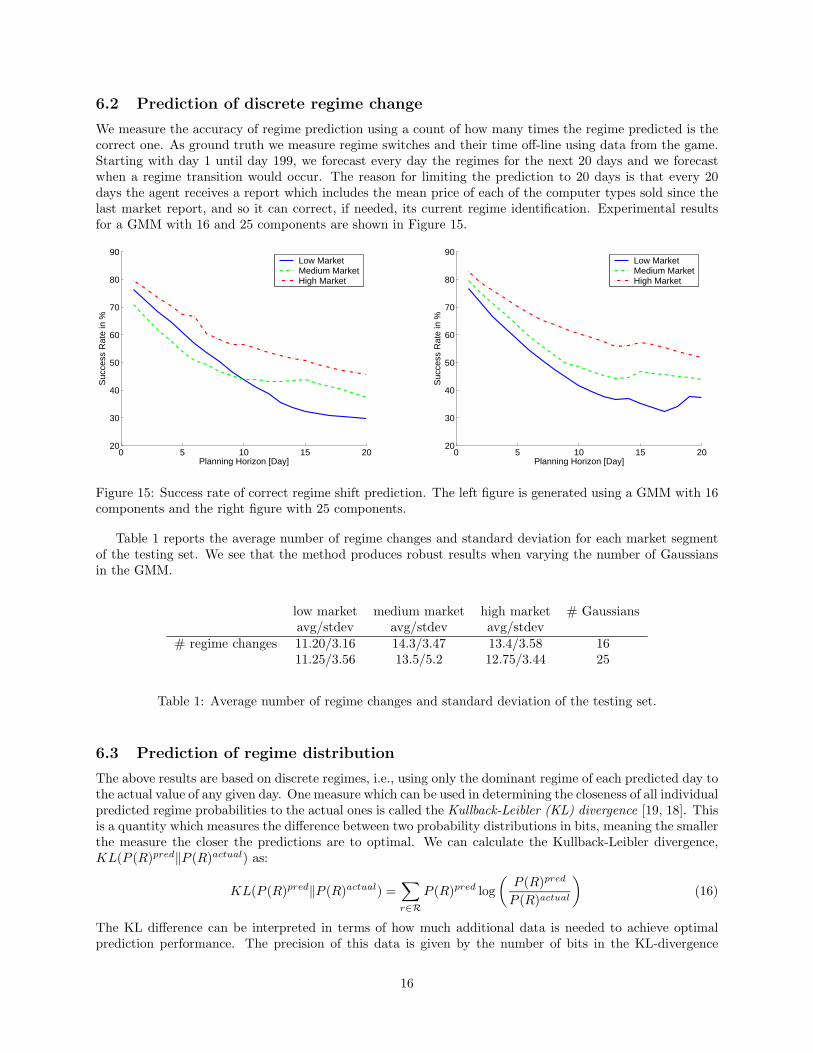
6.2 Prediction of discrete regime change

We measure the accuracy of regime prediction using a count of how many times the regime predicted is thecorrect one. As ground truth we measure regime switches and their time off-line using data from the game.Starting with day 1 until day 199, we forecast every day the regimes for the next 20 days and we forecastwhen a regime transition would occur. The reason for limiting the prediction to 20 days is that every 20days the agent receives a report which includes the mean price of each of the computer types sold since thelast market report, and so it can correct, if needed, its current regime identification. Experimental resultsfor a GMM with 16 and 25 components are shown in Figure 15.

0 5 10 15 2020

30

40

50

60

70

80

90

Planning Horizon [Day]

Suc

cess

Rat

e in

%

Low MarketMedium MarketHigh Market

0 5 10 15 2020

30

40

50

60

70

80

90

Planning Horizon [Day]

Suc

cess

Rat

e in

%

Low MarketMedium MarketHigh Market

Figure 15: Success rate of correct regime shift prediction. The left figure is generated using a GMM with 16components and the right figure with 25 components.

Table 1 reports the average number of regime changes and standard deviation for each market segmentof the testing set. We see that the method produces robust results when varying the number of Gaussiansin the GMM.

low market medium market high market # Gaussiansavg/stdev avg/stdev avg/stdev

# regime changes 11.20/3.16 14.3/3.47 13.4/3.58 1611.25/3.56 13.5/5.2 12.75/3.44 25

Table 1: Average number of regime changes and standard deviation of the testing set.

6.3 Prediction of regime distribution

The above results are based on discrete regimes, i.e., using only the dominant regime of each predicted day tothe actual value of any given day. One measure which can be used in determining the closeness of all individualpredicted regime probabilities to the actual ones is called the Kullback-Leibler (KL) divergence [19, 18]. Thisis a quantity which measures the difference between two probability distributions in bits, meaning the smallerthe measure the closer the predictions are to optimal. We can calculate the Kullback-Leibler divergence,KL(P (R)pred‖P (R)actual) as:

KL(P (R)pred‖P (R)actual) =∑

r∈R

P (R)pred log

(

P (R)pred

P (R)actual

)

(16)

The KL difference can be interpreted in terms of how much additional data is needed to achieve optimalprediction performance. The precision of this data is given by the number of bits in the KL-divergence

16

measure. For example a 1 bit difference would require an additional binary piece of information [28], like:“Were yesterday’s bids all satisfied?” If the difference between the two distributions is 0 than the predictionsare optimal in sense that all the probabilistic information about pricing behavior is accurate (e.g. thepredicted and actual distributions match).

0 5 10 15 200

0.5

1

1.5

2

2.5

3

3.5

Planning Horizon [Day]

KL−

Div

erge

nce

KLPredReal

KLExpSPredReal

0 5 10 15 200

0.5

1

1.5

2

2.5

3

3.5

Planning Horizon [Day]

KL−

Div

erge

nce

KLPredReal

KLExpSPredReal

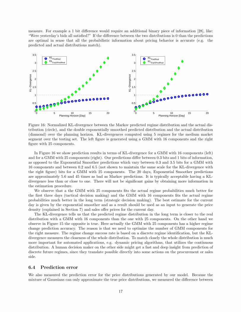
Figure 16: Normalized KL-divergence between the Markov predicted regime distribution and the actual dis-tribution (circle), and the double exponentially smoothed predicted distribution and the actual distribution(diamond) over the planning horizon. KL-divergences computed using 5 regimes for the medium marketsegment over the testing set. The left figure is generated using a GMM with 16 components and the rightfigure with 25 components.

In Figure 16 we show prediction results in terms of KL-divergence for a GMM with 16 components (left)and for a GMM with 25 components (right). Our predictions differ between 0.3 bits and 1 bits of information,as opposed to the Exponential Smoother predictions which vary between 0.3 and 3.5 bits for a GMM with16 components and between 0.2 and 6.5 (not shown to maintain the same scale for the KL-divergence withthe right figure) bits for a GMM with 25 components. The 20 days, Exponential Smoother predictionsare approximately 5.6 and 45 times as bad as Markov predictions. It is typically acceptable having a KL-divergence less than or close to one. There will not be significant gains by obtaining more information inthe estimation procedure.

We observe that a the GMM with 25 components fits the actual regime probabilities much better forthe first three days (tactical decision making) and the GMM with 16 components fits the actual regimeprobabilities much better in the long term (strategic decision making). The best estimate for the currentday is given by the exponential smoother and as a result should be used as an input to generate the pricedensity (explained in Section 7) and sales offer prices for the current day.

The KL-divergence tells us that the predicted regime distribution in the long term is closer to the realdistribution with a GMM with 16 components than the one with 25 components. On the other hand weobserve in Figure 15 the opposite is true. Here actually the GMM with 25 components has a higher regimechange prediction accuracy. The reason is that we need to optimize the number of GMM components forthe right measure. The regime change success rate is based on a discrete regime identification, but the KL-divergence measures the closeness of the whole distribution. To match closely the whole distribution is muchmore important for automated applications, e.g. dynamic pricing algorithms, that utilizes the continuousdistribution. A human decision maker on the other side might get a fast and deep insight from prediction ofdiscrete future regimes, since they translate possible directly into some actions on the procurement or salesside.

6.4 Prediction error

We also measured the prediction error for the price distributions generated by our model. Because themixture of Gaussians can only approximate the true price distributions, we measured the difference between

17

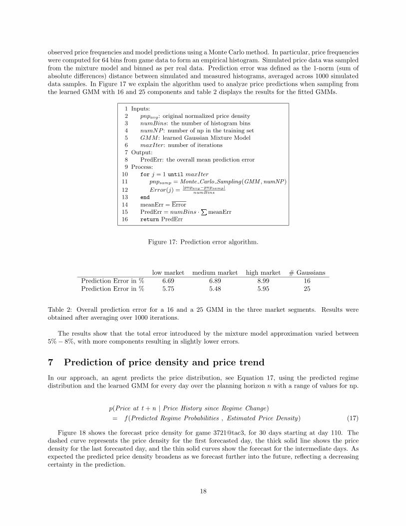
observed price frequencies and model predictions using a Monte Carlo method. In particular, price frequencieswere computed for 64 bins from game data to form an empirical histogram. Simulated price data was sampledfrom the mixture model and binned as per real data. Prediction error was defined as the 1-norm (sum ofabsolute differences) distance between simulated and measured histograms, averaged across 1000 simulateddata samples. In Figure 17 we explain the algorithm used to analyze price predictions when sampling fromthe learned GMM with 16 and 25 components and table 2 displays the results for the fitted GMMs.

1 Inputs:2 pnpavg: original normalized price density3 numBins: the number of histogram bins4 numNP : number of np in the training set5 GMM : learned Gaussian Mixture Model6 maxIter: number of iterations7 Output:8 PredErr: the overall mean prediction error9 Process:

10 for j = 1 until maxIter

11 pnpsamp = Monte Carlo Sampling(GMM , numNP)

12 Error(j) =|pnpavg−pnpsamp|

numBins

13 end

14 meanErr = Error15 PredErr = numBins ·

PmeanErr

16 return PredErr

Figure 17: Prediction error algorithm.

low market medium market high market # GaussiansPrediction Error in % 6.69 6.89 8.99 16Prediction Error in % 5.75 5.48 5.95 25

Table 2: Overall prediction error for a 16 and a 25 GMM in the three market segments. Results wereobtained after averaging over 1000 iterations.

The results show that the total error introduced by the mixture model approximation varied between5% − 8%, with more components resulting in slightly lower errors.

7 Prediction of price density and price trend

In our approach, an agent predicts the price distribution, see Equation 17, using the predicted regimedistribution and the learned GMM for every day over the planning horizon n with a range of values for np.

p(Price at t + n | Price History since Regime Change)

= f(Predicted Regime Probabilities , Estimated Price Density) (17)

Figure 18 shows the forecast price density for game 3721@tac3, for 30 days starting at day 110. Thedashed curve represents the price density for the first forecasted day, the thick solid line shows the pricedensity for the last forecasted day, and the thin solid curves show the forecast for the intermediate days. Asexpected the predicted price density broadens as we forecast further into the future, reflecting a decreasingcertainty in the prediction.

18

0 0.2 0.4 0.6 0.8 1 1.20

0.01

0.02

0.03

0.04

0.05

0.06

Normalized Price (np)

Pro

babi

lity

Den

sity

of n

pDay one forecast distribution

Figure 18: Predicted price density using theMarkov model for game 3721@tac3 from day 110until day 140 in the medium market segment. Thered dashed curve is the price density estimate forthe current day, the black solid curve is the pricedensity estimate for the last day in the planninghorizon, and the green solid curves are the esti-mates for the intermediate days.

115 120 125 130 135 140

−0.14

−0.12

−0.1

−0.08

−0.06

−0.04

−0.02

0

0.02

Day

Pric

e T

rend

5%10%50%Real Mean

Figure 19: Predicted price trend for game3721@tac3 from day 110 until day 140 in themedium market segment. The solid curve is thereal mean price and the dashed and dotted curvesare predicted price trends based on the 5%, 10%and 50% percentile on the predicted price density.

We can also compare the actual price trends with our predictions. Figure 19 shows the real mean pricetrend along with forecast price trends based on the different predictors, e.g. the 5%, 10% and the 50%percentiles. All the curves in the figure represent a relative price trend – to better compare the differentpredictors which each other graphically, we subtracted from each forecasted value the first predicted value,so that they all start at zero.

8 Conclusions and future work

We have presented an approach for identifying and predicting market conditions in markets for durablegoods. We have demonstrated the effectiveness of our approach using games played in the semi-finals andfinals from TAC SCM 2005. An advantage of the proposed method is that it works in any market for durablegoods, since the computational process is completely data driven and that no classification of the marketstructure (monopoly vs competitive, etc) is needed.

8.1 Contributions

Our approach recognizes that different market situations have qualitative differences that can be used toguide the strategic and tactical behavior of an agent. Unlike regression-based methods that try to predictprices directly from demand and other observable factors, our approach recognizes that prices are alsoinfluenced by non-observable factors, such as the inventory positions of other agents. Our approach alsolearns the dynamics and durations of price regimes, and when to expect a shift in the dominant regime.This is important information that is difficult to represent with regression-based methods. For example,regression in an expanding market (where prices increase) will extrapolate increasing prices using the slopeof recent price data. On the other hand, the regime approach can learn that expansion (or scarcity) regimesare typically limited in duration and predictably followed by other regimes. When prices are increasing, itis more important to know if prices will fall by the end of the planning horizon, which can be invaluableinformation for a decision maker. Our method can enable an agent to anticipate and prepare for regimechanges, for example by building up inventory in anticipation of better prices in the future or by selling inanticipation of an upcoming oversupply situation.

19

8.2 Future directions

Our approach maintains the uncertainty in price prediction by maintaining a price distribution, which allowsan agent to avoid over-committing to risky decisions. We intend to apply our method in other domains wherepredicting price distributions appears fruitful, including data from Amazon.com, eBay.com, and financialapplications like stock tracking and forecasting.

We have implemented the regime identification and prediction method in a TAC SCM agent and inte-grated it into the overall decision making process. We are currently using regime predictions for strategicdecision making in the sales component of our agent. We have begun to design an algorithm that use regimepredictions for tactical decision making as well. Ultimately, we plan to combine probability information sup-plied by the algorithm with information about possible consequences of actions to optimize decision making.In particular, we would like to use the whole regime-based predicted price density to optimize tactical salespricing by maximizing expected utility [31].

In addition, we plan to apply we plan to apply reinforcement learning [29] to map economic regimesto internal operational regimes and operational regimes to actions, such as procurement and productionscheduling. Under operational regimes we understand a state which includes which actions to take nextwhile knowing the current regime and receiving the regime forecast.

9 Appendix: Summary of notation

Symbol Definition

np Normalized pricenp Mid-range normalized pricenpmin Smoothed minimum normalized pricenpmax Smoothed maximum normalized pricenp Smoothed mid-range normalized priceα Smoothing coefficientp(np) Density of the normalized priceGMM Gaussian Mixture ModelN Number of Gaussians of the GMMp(np|ci) Density of the normalized price, np, given i-th Gaussian of the

GMMµi Mean of i-th Gaussian of the GMMσi Standard deviation of i-th Gaussian of the GMM

P (ci) Prior probability of i-th Gaussian of the GMMP (ci|np) Posterior probability of the i-th Gaussian of the GMM given a

normalized price np~η(np) N-dimensional vector with posterior probabilities, P (ci|np), of

the GMMM Number of regimesRk k-th Regime, k = 1, · · · , M

P(c|r) Conditional probability matrix (N rows and M columns) re-sulting from k-means clustering

p(np|Rk) Density of the normalized price np given a regime Rk

P (Rk|np) Probability of regime Rk given a normalized price npt Current timet0 Time of last regime changeTpredict(rt+1|rt) Markov transition matrix

References

[1] Michael Benisch, Amy Greenwald, Ioanna Grypari, Roger Lederman, Victor Naroditskiy, and MichaelTschantz. Botticelli: A supply chain management agent designed to optimize under uncertainty. ACM

20

Trans. on Comp. Logic, 4(3):29–37, 2004.

[2] P. Berry, K. Conley, M. Gervasio, B. Peintner, T. Uribe, and N. Yorke-Smith. Deploying a personalizedtime management agent. In Proc. of the Fifth Int’l Conf. on Autonomous Agents and Multi-AgentSystems, Hakodate, Japan, May 2006.

[3] Urszula Chajewska, Daphne Koller, and Dirk Ormoneit. Learning an agent’s utility function by ob-serving behavior. In Proc. of the 18th Int’l Conf. on Machine Learning, pages 35–42, Lafayette, June2001.

[4] John Collins, Raghu Arunachalam, Norman Sadeh, Joakim Ericsson, Niclas Finne, and Sverker Janson.The Supply Chain Management Game for the 2005 Trading Agent Competition. Technical ReportCMU-ISRI-04-139, Carnegie Mellon University, Pittsburgh, PA, December 2004.

[5] John Collins, Corey Bilot, Maria Gini, and Bamshad Mobasher. Decision processes in agent-basedautomated contracting. IEEE Internet Computing, 5(2):61–72, March 2001.

[6] John Collins, Wolfgang Ketter, and Maria Gini. A multi-agent negotiation testbed for contracting taskswith temporal and precedence constraints. Int’l Journal of Electronic Commerce, 7(1):35–57, 2002.

[7] CombineNet. Sourcing solutions. http://www.combinenet.com/sourcing solutions/, 2006.

[8] A. P. Dempster, N. M. Laird, and D. B. Rubin. Maximum likelihood from incomplete data via the EMalgorithm. J. of the Royal Stat. Soc., Series B, 39(1):1–38, 1977.

[9] Rayid Ghani. Price prediction and insurance for online auctions. In Int’l Conf. on Knowledge Discoveryin Data Mining, pages 411–418, Chicago, Illinois, August 2005.

[10] Anindya Ghose, Michael D. Smith, and Rahul Telang. Internet exchanges for used books: An empiricalanalysis of product cannibalization and welfare impact. Information Systems Research, 17(1):3–19,2006.

[11] Minghua He, Alex Rogers, Esther David, and Nicholas R. Jennings. Designing and evaluating anadaptive trading agent for supply chain management applications. In IJCAI 2005 Workshop on TradingAgent Design and Analysis, pages 35–42, Edinburgh, Scotland, August 2005.

[12] I2. Next-generation planning. http://i2.com/solution library/ng planning.cfm, 2006.

[13] Michael Kearns and Luis Ortiz. The Penn-Lehman Automated Trading Project. IEEE IntelligentSystems, pages 22–31, 2003.

[14] Jeffrey O. Kephart, James E. Hanson, and Amy R. Greenwald. Dynamic pricing by software agents.Computer Networks, 32(6):731–752, 2000.

[15] Wolfgang Ketter, Elena Kryzhnyaya, Steven Damer, Colin McMillen, Amrudin Agovic, John Collins,and Maria Gini. MinneTAC sales strategies for supply chain TAC. In Int’l Conf. on Autonomous Agentsand Multi-Agent Systems, pages 1372–1373, New York, July 2004.

[16] Christopher Kiekintveld, Yevgeniy Vorobeychik, and Michael P. Wellman. An Analysis of the 2004Supply Chain Management Trading Agent Competition. In IJCAI 2005 Workshop on Trading AgentDesign and Analysis, pages 61–70, Edinburgh, Scotland, August 2005.

[17] Christopher Kiekintveld, Michael P. Wellman, Satinder Singh, Joshua Estelle, Yevgeniy Vorobeychik,Vishal Soni, and Matthew Rudary. Distributed feedback control for decision making on supply chains.In Int’l Conf. on Automated Planning and Scheduling, pages 384–392, Whistler, BC, Canada, June2004.

[18] Solomon Kullback. Information Theory and Statistics. Dover Publications, New York, 1959.

21

[19] Solomon Kullback and Richard A. Leibler. On information and sufficiency. Annals of MathematicalStatistics, 22:79–86, 1951.

[20] Richard Lawrence. A machine learning approach to optimal bid pricing. In 8th INFORMS ComputingSociety Conf. on Optimization and Computation in the Network Era, pages 1–22, Arizona, January2003.

[21] Bill Mark and Raymond C. Perrault. Calo: Cognitive assistant that learns and organizes.http://www.ai.sri.com/project/CALO, 2006.

[22] Cade Massey and George Wu. Detecting regime shifts: The causes of under- and overestimation.Management Science, 51(6):932–947, 2005.

[23] Andrew Ng and Stuart Russell. Algorithms for inverse reinforcement learning. In Proc. of the 17th Int’lConf. on Machine Learning, pages 663–670, Palo Alto, June 2000.

[24] Denise R. Osborn and Marianne Sensier. The prediction of business cycle phases: financial variablesand international linkages. National Institute Econ. Rev., 182(1):96–105, 2002.

[25] David Pardoe and Peter Stone. Bidding for Customer Orders in TAC SCM: A Learning Approach. InWorkshop on Trading Agent Design and Analysis at AAMAS, pages 52–58, New York, July 2004.

[26] Koen Pauwels and Dominique Hanssens. Windows of Change in Mature Markets. In European MarketingAcademy Conf., Braga, Portugal, May 2002.

[27] Tuomas Sandholm. Expressive commerce and its application to sourcing. In Proc. of the Twenty-FirstNational Conference on Artificial Intelligence, pages 1736–1743, Boston, MA, July 2006. AAAI.

[28] Claude E. Shannon. A mathematical theory of communication. Bell System Technical Journal,27(3):379–423 and 623–656, July and October 1948.

[29] Richard S. Sutton and Andrew G. Barto. Reinforcement Learning - An Introduction. The MIT Press,Cambridge, 1998.

[30] D. Titterington, A. Smith, and U. Makov. Statistical Analysis of Finite Mixture Distributions. Wiley,New York, 1985.

[31] John von Neumann and Oskar Morgenstern. Theory of Games and Economic Behavior. PrincetonUniversity Press, 2nd edition, Princeton, N.J., 1947.

[32] Michael P. Wellman, Daniel M. Reeves, Kevin M. Lochner, and Yevgeniy Vorobeychik. Price predictionin a trading agent competition. Journal of Artificial Intelligence Research, 2003.

[33] Dongmo Zhang, Kanghua Zhao, Chia-Ming Liang, Gonelur Begum Huq, and Tze-Haw Huang. Strategictrading agents via market modeling. SIGecom Exchanges, 4(3):46–55, 2004.

22