VAR Forecasting

8/13/2019 VAR Forecasting

http://slidepdf.com/reader/full/var-forecasting 1/27

3. VAR: FORECASTING AND IMPULSE RESPONSE

FUNCTIONS

1



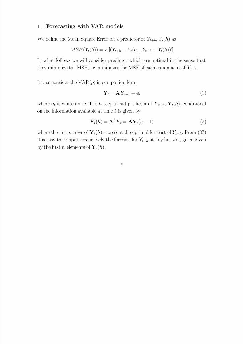
1 Forecasting with VAR models

We define the Mean Square Error for a predictor of Y t+h, Y t(h) as

MSE (Y t(h)) = E [(Y t+h − Y t(h))(Y t+h − Y t(h))]

In what follows we will consider predictor which are optimal in the sense that

they minimize the MSE, i.e. minimizes the MSE of each component of Y t+h.

Let us consider the VAR( p) in companion formYt = AYt−1 + et (1)

where et is white noise. The h-step ahead predictor of Yt+h, Yt(h), conditional

on the information available at time t is given by

Yt(h) = AhYt = AYt(h

−1) (2)

where the first n rows of Yt(h) represent the optimal forecast of Y t+h. From (37)

it is easy to compute recursively the forecast for Y t+h at any horizon, given given

by the first n elements of Yt(h).

2



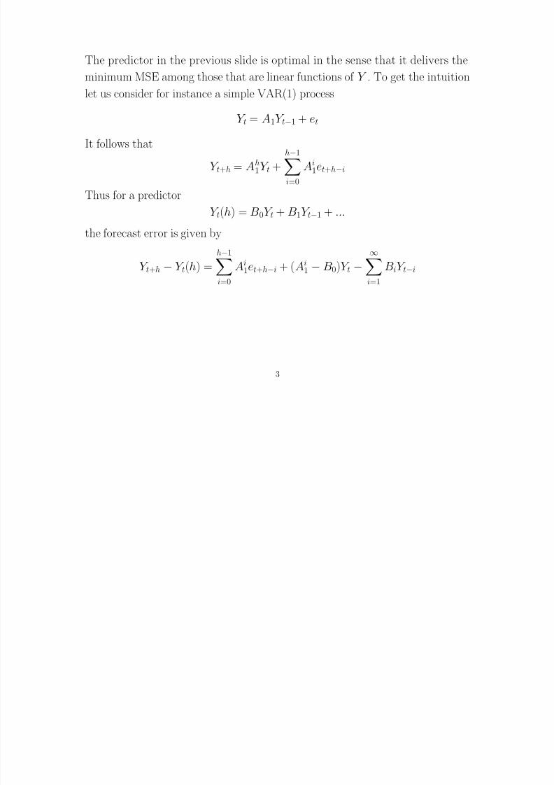
The predictor in the previous slide is optimal in the sense that it delivers the

minimum MSE among those that are linear functions of Y . To get the intuition

let us consider for instance a simple VAR(1) process

Y t = A1Y t−1 + et

It follows that

Y t+h = Ah1Y t +

h−1

i=0Ai

1et+h−i

Thus for a predictorY t(h) = B0Y t + B1Y t−1 + ...

the forecast error is given by

Y t+h − Y t(h) =h−1

i=0Ai

1et+h−i + (Ai1 − B0)Y t −

∞

i=1BiY t−i

3



The MSE is given by

MSE (Y t(h)) = E h−1

i=0A1et+h−i

h−1i=0

A1et+h−i

+

E

Ah − B0

Y t −

∞i=1

BiY t−i

(Ah − B0)Y t −

∞i=1

BiY t−i

Clearly the MSE is minimal for B0 = Ah1 and Bi = 0.

4



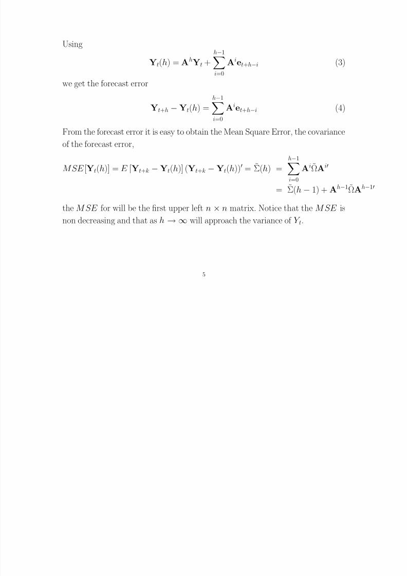
Using

Yt(h) = AhYt +h−1

i=0

Aiet+h

−i (3)

we get the forecast error

Yt+h − Yt(h) =h−1i=0

Aiet+h−i (4)

From the forecast error it is easy to obtain the Mean Square Error, the covariance

of the forecast error,

MSE [Yt(h)] = E [Yt+k − Yt(h)] (Yt+k − Yt(h)) = Σ(h) =h−1i=0

AiΩAi

= Σ(h− 1) + Ah−1ΩAh−1

the M SE for will be the first upper left n × n matrix. Notice that the M SE isnon decreasing and that as h →∞ will approach the variance of Y t.

5



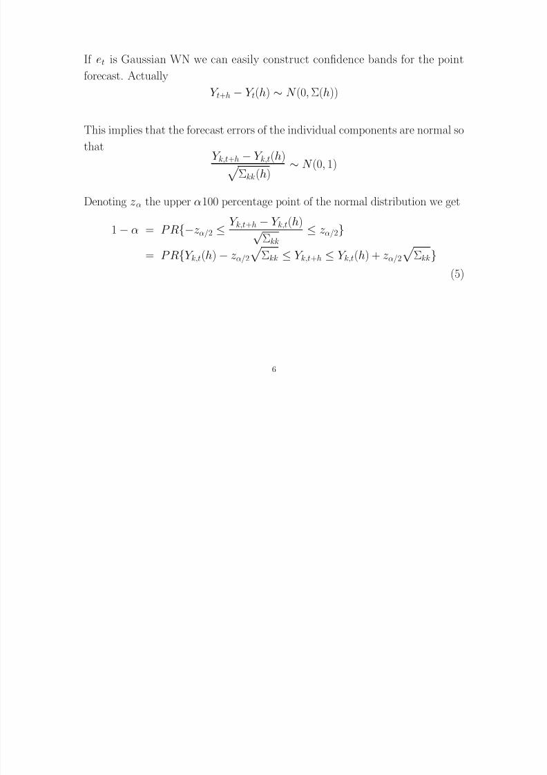
If et is Gaussian WN we can easily construct confidence bands for the point

forecast. Actually

Y t+h − Y t(h) ∼ N (0, Σ(h))

This implies that the forecast errors of the individual components are normal so

thatY k,t+h − Y k,t(h)

Σkk(h)∼ N (0, 1)

Denoting z α the upper α100 percentage point of the normal distribution we get

1 − α = P R−z α/2 ≤ Y k,t+h − Y k,t(h)√

Σkk

≤ z α/2

= P RY k,t(h)− z α/2

Σkk ≤ Y k,t+h ≤ Y k,t(h) + z α/2

Σkk

(5)

6



Hence a (1 − α)100% interval forecast, h periods ahead, for the kth component

of Y t is

[Y k,t(h) − z α/2

Σkk, Y k,t(h) + z α/2

Σkk] (6)In case et is not Gaussian we can still construct confidence bands for point forecast

using the methods described for impulse response functions.

7



• What is the difference between in-sample and out-of-sample forecasting?

• How do we perform out-of-sample forecast? Suppose we have data for a sampleof length T . We proceed as follows:

1. We use the first T 0 observation to estimate the VAR and we forecast h periods

ahead.

2. We update the sample with one observation (the length of the sample is now

T 0 + 1) and we perform the h periods ahead forecast.

3. We repeat step 2 for all the forecasting sample period up to the last date in

the sample with one observation (the length of the sample is now T 0 +1) and

we perform the h periods ahead forecast.

8



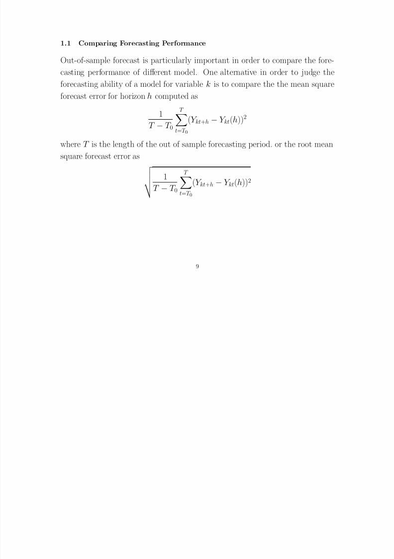
1.1 Comparing Forecasting Performance

Out-of-sample forecast is particularly important in order to compare the fore-

casting performance of different model. One alternative in order to judge the

forecasting ability of a model for variable k is to compare the the mean square

forecast error for horizon h computed as

1

T − T 0

T

t=T 0

(Y kt+h − Y kt(h))2

where T is the length of the out of sample forecasting period. or the root mean

square forecast error as

1

T − T 0

T t=T 0

(Y kt+h − Y kt(h))2

9



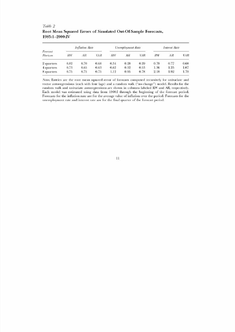
1.2 Application: Stock and Watson Monetary VAR

•SW consider a trivariate VAR(4) model including inflation unemployment and

the short term interest rate.

• The sample spans from 1960:I-2000:IV. The authors use data from 1960:I to

1984:IV to estimate the VAR and then use the sample 1985:I-2000:IV to compute

the root mean square forecast error of the forecast.

• In addition, the authors estimate compute the RMSE for a univariate AR(4)

forecast and a naive random walk (no change) forecast.

10



11



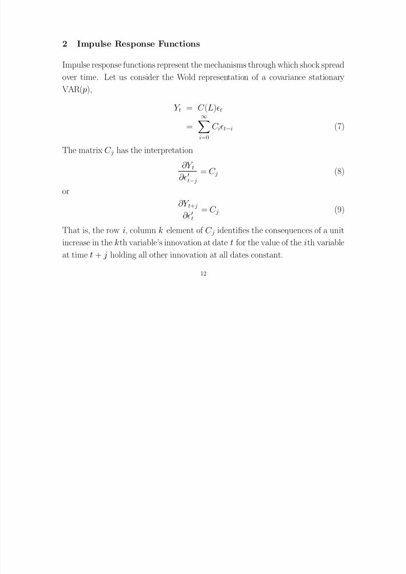
2 Impulse Response Functions

Impulse response functions represent the mechanisms through which shock spread

over time. Let us consider the Wold representation of a covariance stationary

VAR( p),

Y t = C (L)t

=∞

i=0C it−i (7)

The matrix C j has the interpretation

∂Y t∂t− j

= C j (8)

or

∂Y t+ j

∂t = C j (9)

That is, the row i, column k element of C j identifies the consequences of a unit

increase in the kth variable’s innovation at date t for the value of the ith variable

at time t + j holding all other innovation at all dates constant.

12



Example 1 Let us assume that the estimated matrix of VAR coefficients is

A = 0.8 0.1

−0.2 0.5 (10)

with eigenvalues 0.8562 and 0.4438. We generate impulse response functions of

the Wold representation

C j = A j

13



Figure 3: Impulse response functions

14



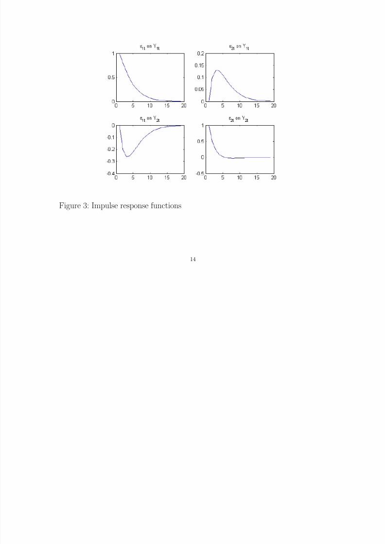
Example 2 Let us now assume that the second variable does not Granger cause

the first one so that

A =

0.8 0−0.2 0.5

(11)

with eigenvalues 0.8 and 0.5. Impulse response functions are plotted in the next

figure

15



Figure 4: Impulse response functions when the second variable does not Granger

cause the first one.

16



2.1 Error Bands for Impulse Response Functions

To make inference about the effects of the shocks we need to quantify the uncer-

tainty around the point estimate, we need the confidence bands for the impulseresponse functions. We will see three different methods to construct confidence

bands

1. Asymptotic bands

2. Montecarlo bands

3. Boostrap bands

17



2.2 Error Bands for Impulse Response Functions: Asymptotic

Hamilton (1994) shows that

(T )(vec( C s) − vec(C s))

L→N

0, Gs(Ω ⊗ Q−1)G

s

where

Gs =s

i=1

C i−1 ⊗ (0n1C s−i C s−i−1 . . . C s−i− p+1)

is of dimension n2

× np. Standard errors for an estimated impulse responsecoefficient are given by the square root of the associated diagonal element of

Gs,T (ΩT ⊗ Q−1T )G

s,T

where

QT = (1/T )T

t=1

X tX t and X t = [Y t−1,...,Y t

−1]

.

18



2.3 Error Bands for Impulse Response Functions: Montecarlo

Montecarlo method proceeds as follows.

1. Draw πl from N (π, Ω ⊗ Q−1).

2. compute C (L)l.

3. Repeat 1-2 M (with M big, i.e.1000) times.

4. For all the elements C i,j,h, i , j = 1,...,n,h = 1, 2,... of the impulse response

functions collect the αth and 1 − αth percentile across the draws as aconfidence interval for C i,j,h.

19



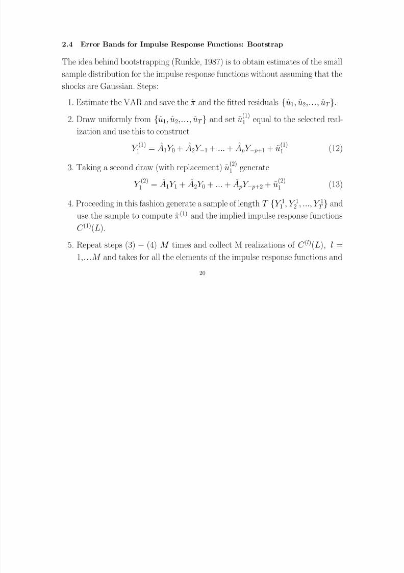
2.4 Error Bands for Impulse Response Functions: Bootstrap

The idea behind bootstrapping (Runkle, 1987) is to obtain estimates of the small

sample distribution for the impulse response functions without assuming that theshocks are Gaussian. Steps:

1. Estimate the VAR and save the π and the fitted residuals u1, u2,..., uT .

2. Draw uniformly from u1, u2,..., uT and set u(1)1 equal to the selected real-

ization and use this to construct

Y (1)1 = A1Y 0 + A2Y −1 + ... + A pY − p+1 + u(1)1 (12)

3. Taking a second draw (with replacement) u(2)1 generate

Y (2)1 = A1Y 1 + A2Y 0 + ... + A pY − p+2 + u

(2)1 (13)

4. Proceeding in this fashion generate a sample of length T

Y 11 , Y 12 , ..., Y 1T

and

use the sample to compute π(1) and the implied impulse response functionsC (1)(L).

5. Repeat steps (3) − (4) M times and collect M realizations of C (l)(L), l =

1,...M and takes for all the elements of the impulse response functions and

20



for all the horizons the αth and 1 − αth percentile to construct confidence

bands.

21



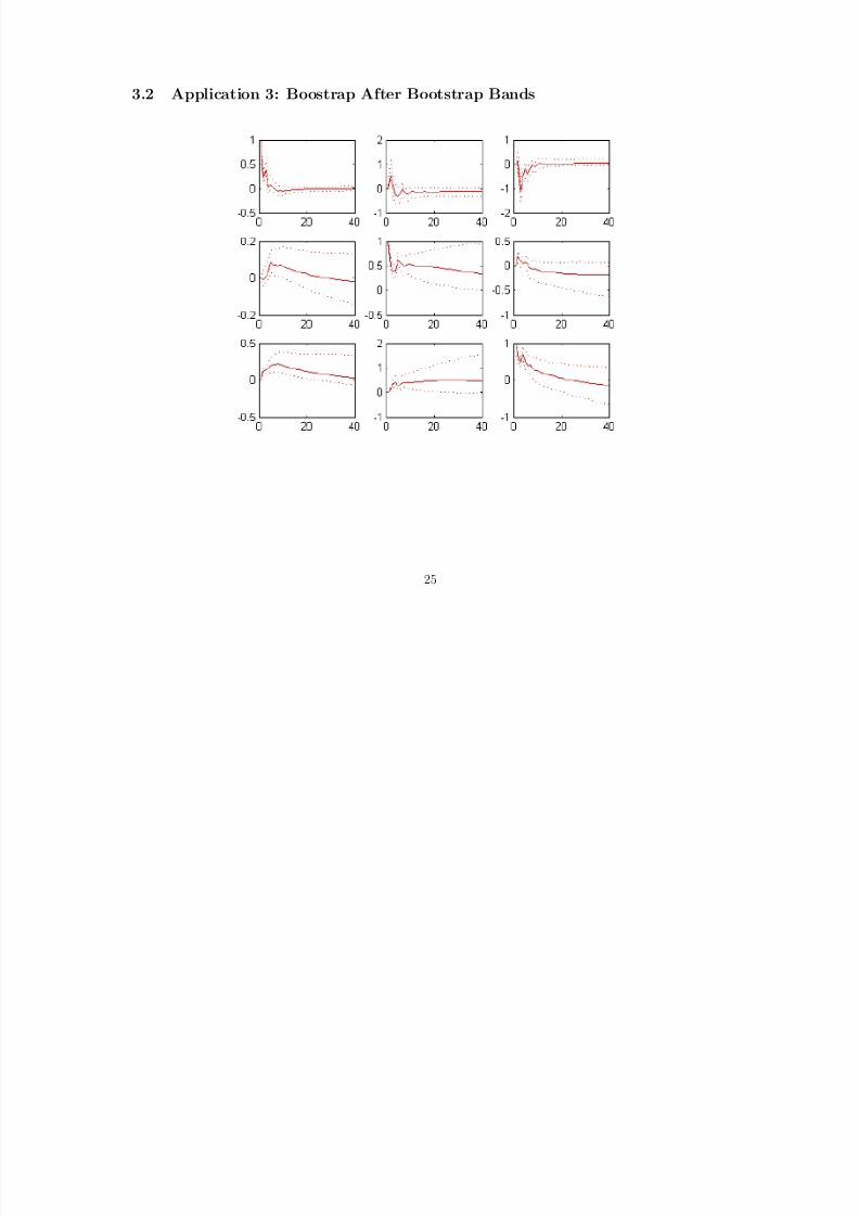
2.5 Error Bands for Impulse Response Functions: Bootstrap after Bootstrap

The bootstrap after bootstrap method (Kilian 1998) is a way to generate bias

corrected confidence bands and it works as follows.

1. Estimate the VAR using OLS.

2. Generate 1000 draws for impulse response functions using bootstrap.

3. Correct the OLS estimator for the bias and get the bias corrected estimatorˆβ ∗ =

ˆβ −Bias where Bias =

¯β

−ˆβ where

¯β

is the average of the parameterover the bootstrap replications.

4. Use β ∗ to generate 2000 new bootstrap correcting each OLS estimate for the

previously estimated bias.

22



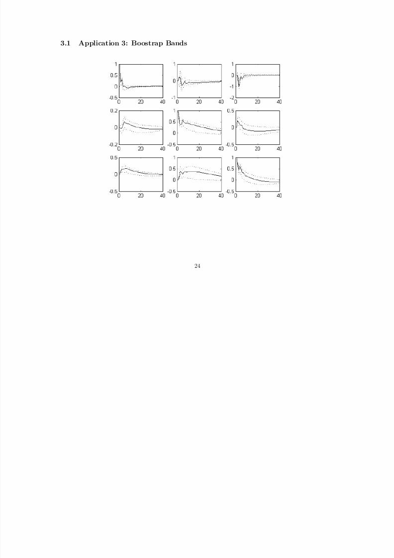
3 Application 3: A Monetary VAR

We estimate the standard monetary VAR which includes real output growth,

the inflation rate and the federal funds rate. These three variables are the core

variables for monetary policy analysis in VAR models. Data are taken from the

St.Louis Fed FREDII database.

23



3.1 Application 3: Boostrap Bands

24



3.2 Application 3: Boostrap After Bootstrap Bands

25



4 Cumulated impulse response functons

Suppose Y t is a vector of trending variables (i.e. log prices and output) so we

consider the first difference to reach stationarity. So the model is

∆Y t = (1 − L)Y t = C (L)εt

We know hoe to estimate, interpret, and conduct inference on C (L). But suppose

we are interested in the response of the levels of Y t rather than their first differences

(the level of and prices rather than their growth rates). How can we find these

responses? We transform the model

Y t = Y t−1 + C (L)εt

The effect of εt on Y t is C 0. Now substituting forward we obtain

Y t+1 = Y t−1 + C (L)εt + C (L)εt+1

= Y t−1 + C 0εt+1 + (C 0 + C 1)εt + ...(14)

and for two periods ahead

Y t+2 = Y t−1 + C (L)εt + C (L)εt+1 + C (L)εt+2

26



= Y t−1 + C 0εt+2 + (C 0 + C 1)εt+1 + (C 0 + C 1 + C 2)εt+1...

(15)

so the effect of εt on Y t+1 are (C 0 + C 1) and on Y t+2 is (C 0 + C 1 + C 2). In general

the effects of εt on Y t+ j are

C j = C 0 + C 1 + ... + C j

defined as cumulated impulse response functions.

27

Documents

VAR Forecasting