Big Data techniques for Solar Power Forecasting

By

Rui Miguel da Cunha Nunes

Dissertation of Master in Data analytics and Decision Support Systems

Supervised by

Ricardo Jorge Gomes de Sousa Bento BessaJoão Manuel Portela da Gama

2017

Biographical Note

Rui Miguel da Cunha Nunes was born in June 30th 1981 in Viseu, Portugal. Followinghis high school graduation in electronics, he proceeded with his education at Aveiro’sUniversity, completing his degree in Applied Mathematics and Computing in July 2005.After graduation, he decided to apply the acquired knowledge in the corporative world.All his experience is related to software developing in all of their stages. These experi-ences vary in the technologies as well in the business. In 2014 he decided to enrol in theMaster in Data Analytics and Decision Support Systems, to proceed with his academiccourse trying to conjugate both his work experience as well his undergraduate academiccourse.

i

Acknowledgements

First and foremost I thank my supervisors for all their help and incentive. Ricardo Bessafor proposed this theme that inspired me from the start. Professor João Gama for all thesupport that he provided. Special thanks to Laura Cavalcante that shared her knowledgein the LASSO-VAR problem.

I would like to thank my family for all the patient and all the missing hours away fromhome and some bad humor from the lake of sleep. Thank my boys Miguel e Pedro, forunderstanding all the missed hours that I was not with you and all joyful moments that Iwas not there to see.

ii

Abstract

With the growth of social awareness for environmental issues, came a new and importantproblem to the discussion, related to renewable energies. Although this kind of energyproduction is already in an advanced state of development there are some issues that stillneed to be studied and perfected on the real production environment. The Photovoltaicproduction is gain some importance but the prediction of this kind of energy still needa boost in their performance. The SMART Grid projects brought this issues to anotherlevel where the importance of these predictions needs to be as accurate as possible, butthey brought another problem, how to accurate this prediction with all data that this kindof problems is associated with. There are some accurate models for a single locationprediction but we involving multiple locations in one problem we need to have somecomputational power. Big Data techniques such the Convex optimization are a field thatis important to explore since these techniques applied with the parallel computer pro-gramming paradigm can bring that computational power, and more accurate models canbe trained faster.Keywords:Big Data, Convex Optimization, VAR, SMART Grids.

Resumo

Com o crescimento da consciência social para questões ambientais, surgiu um novo eimportante problema para a discussão, relacionada às energias renováveis. Embora estetipo de produção de energia já esteja em um estado avançado de desenvolvimento, exis-tem algumas questões que ainda precisam ser estudadas e aperfeiçoadas no ambiente deprodução real. A produção fotovoltaica ganha alguma importância, mas a previsão destetipo de energia ainda precisa de um impulso no desempenho. Os projetos SMART Gridtrouxeram esses problemas para outro nível, onde a importância dessas previsões precisaser o mais preciso possível, mas eles trouxeram outro problema, como precisão dessaprevisão com todos os dados associados a esse tipo de problemas. Existem alguns mode-los precisos para uma previsão de localização única, mas envolvendo múltiplos locais emum único problema, precisamos ter algum poder computacional. As técnicas Big Data,tais como a Otimização Convexa, são um campo que é importante explorar, uma vez queessas técnicas aplicadas com o paradigma paralelo de programação de computadores po-dem trazer esse poder computacional e modelos mais precisos podem ser treinados maisrapidamente.Palavras-chave: Big Data, optimização convexa, VAR, SMART Grids.

Abbreviations

OLS Ordinary Least SquaresLASSO Least Absolute Shrinkage and SelectionML Machine LearningNWP Numerical Weather PredictionMOS Model Output StatisticsNN Neural NetworksANN Artificial Neural NetworksAR AutoregressiveARMA Autoregressive and Moving AverageEB Energy BoxDTC Distribution Transformer ControllerVAR Vector AutoregressiveANN-GA Artificial Neural Networks trained with genetic algorithmsk-NN k-nearest neighborsSVM Support Vector MachinesESO Expected Separable OverapproximationIEA PVPS Photovoltaic Power Systems ProgrammeECMWF European Centre for Medium-Range Weather ForecastsHMM Hidden Markov modelPV PhotovoltaicNARX Nonlinear Autoregressive with eXogenous inputs

ii

Nomenclature

WN(σ) White Noise with mean zero and variance σ`p p-Norm equivalent to ‖.‖ppt+k|t, j Prediction on k − ahead step on site jdoyk Day of the year of element khk Time of the day of element k

iii

Contents

Nota Biográfica i

Acknowledgements ii

Abbreviations ii

Nomenclature iii

1 Introduction 11.1 Motivation . . . . . . . . . . . . . . . . . . . . . . . . . . . . . . . . . . 21.2 Problem Definition . . . . . . . . . . . . . . . . . . . . . . . . . . . . . 31.3 Organization . . . . . . . . . . . . . . . . . . . . . . . . . . . . . . . . . 4

2 State of the art 52.1 Solar Power predictions . . . . . . . . . . . . . . . . . . . . . . . . . . . 5

2.1.1 Clear Sky models . . . . . . . . . . . . . . . . . . . . . . . . . . 52.1.2 Physical . . . . . . . . . . . . . . . . . . . . . . . . . . . . . . . 62.1.3 Statistical . . . . . . . . . . . . . . . . . . . . . . . . . . . . . . 72.1.4 Hybrid . . . . . . . . . . . . . . . . . . . . . . . . . . . . . . . 82.1.5 Spatio-temporal . . . . . . . . . . . . . . . . . . . . . . . . . . . 9

2.2 VAR . . . . . . . . . . . . . . . . . . . . . . . . . . . . . . . . . . . . . 102.3 `p Regularization . . . . . . . . . . . . . . . . . . . . . . . . . . . . . . 10

2.3.1 LASSO . . . . . . . . . . . . . . . . . . . . . . . . . . . . . . . 112.4 Convex Optimization . . . . . . . . . . . . . . . . . . . . . . . . . . . . 122.5 Convex Optimization Algorithms . . . . . . . . . . . . . . . . . . . . . . 132.6 Summary . . . . . . . . . . . . . . . . . . . . . . . . . . . . . . . . . . 20

3 Contributions to LASSO-VAR Model Fitting 223.1 Algorithms . . . . . . . . . . . . . . . . . . . . . . . . . . . . . . . . . 23

3.1.1 Shotgun . . . . . . . . . . . . . . . . . . . . . . . . . . . . . . . 243.1.2 GRock . . . . . . . . . . . . . . . . . . . . . . . . . . . . . . . 26

3.2 Summary . . . . . . . . . . . . . . . . . . . . . . . . . . . . . . . . . . 28

iv

4 Case Study 294.1 Data . . . . . . . . . . . . . . . . . . . . . . . . . . . . . . . . . . . . . 294.2 Sub-problem . . . . . . . . . . . . . . . . . . . . . . . . . . . . . . . . 31

4.2.1 RMSE . . . . . . . . . . . . . . . . . . . . . . . . . . . . . . . . 314.2.2 Forecast . . . . . . . . . . . . . . . . . . . . . . . . . . . . . . . 36

4.3 VAR . . . . . . . . . . . . . . . . . . . . . . . . . . . . . . . . . . . . . 414.3.1 RMSE . . . . . . . . . . . . . . . . . . . . . . . . . . . . . . . . 414.3.2 Forecast . . . . . . . . . . . . . . . . . . . . . . . . . . . . . . . 48

5 Conclusions and Future work 545.1 Conclusions . . . . . . . . . . . . . . . . . . . . . . . . . . . . . . . . . 545.2 Future Work . . . . . . . . . . . . . . . . . . . . . . . . . . . . . . . . . 60

5.2.1 Shotgun . . . . . . . . . . . . . . . . . . . . . . . . . . . . . . . 605.2.2 GRock . . . . . . . . . . . . . . . . . . . . . . . . . . . . . . . 605.2.3 General . . . . . . . . . . . . . . . . . . . . . . . . . . . . . . . 60

A RMSE Values 61

B RMSE 67

C Forecast 75

Bibliography 81

v

List of Figures

1.1 GHI . . . . . . . . . . . . . . . . . . . . . . . . . . . . . . . . . . . . . 21.2 Problem illustration . . . . . . . . . . . . . . . . . . . . . . . . . . . . . 3

2.1 LASSO vs. Ridge Regression on R2 . . . . . . . . . . . . . . . . . . . . 122.2 Coordinate Descent . . . . . . . . . . . . . . . . . . . . . . . . . . . . . 14

4.1 Monthly Production . . . . . . . . . . . . . . . . . . . . . . . . . . . . . 304.2 Monthly Production . . . . . . . . . . . . . . . . . . . . . . . . . . . . . 304.3 Shotgun (sub-problem) parallel models RMSE for t + 1 . . . . . . . . . . 324.4 Shotgun (sub-problem) parallel models RMSE for t + 6 . . . . . . . . . . 334.5 GRock (sub-problem) parallel models RMSE for t + 1 . . . . . . . . . . 344.6 GRock (sub-problem) parallel models RMSE for t + 6 . . . . . . . . . . 354.7 EB17 Shotgun (sub-problem) parallel models’step t +1 forecast for 2012-06 364.8 EB17 Shotgun (sub-problem) parallel models’step t +6 forecast for 2012-06 374.9 EB18 Shotgun (sub-problem) parallel models’step t+1 forecast for period

2012-06-28/012-07-02 . . . . . . . . . . . . . . . . . . . . . . . . . . . 374.10 EB18 Shotgun (sub-problem) parallel models’step t+6 forecast for period

2012-06-28/012-07-02 . . . . . . . . . . . . . . . . . . . . . . . . . . . 384.11 EB51 GRock (sub-problem) parallel models’step t + 1 forecast for 2012-02 394.12 EB51 GRock (sub-problem) parallel models’step t + 6 forecast for 2012-02 394.13 EB51 GRock (sub-problem) parallel models’step t + 1 forecast for period

2012-02-02/012-02-04 . . . . . . . . . . . . . . . . . . . . . . . . . . . 404.14 EB51 GRock (sub-problem) parallel models’step t + 6 forecast for period

2012-02-02/012-02-04 . . . . . . . . . . . . . . . . . . . . . . . . . . . 404.15 Shotgun (VAR) parallel models RMSE for t + 1 . . . . . . . . . . . . . . 414.16 Shotgun (VAR) sequential models RMSE for t + 1 . . . . . . . . . . . . . 424.17 Shotgun (VAR) parallel models RMSE for t + 6 . . . . . . . . . . . . . . 434.18 Shotgun (VAR) sequential models RMSE for t + 6 . . . . . . . . . . . . . 444.19 Problem illustration . . . . . . . . . . . . . . . . . . . . . . . . . . . . . 454.20 Problem illustration . . . . . . . . . . . . . . . . . . . . . . . . . . . . . 464.21 Problem illustration . . . . . . . . . . . . . . . . . . . . . . . . . . . . . 474.22 Problem illustration . . . . . . . . . . . . . . . . . . . . . . . . . . . . . 484.23 EB51 Shotgun (VAR) parallel models’step t + 1 forecast for 2012-06 . . . 49

vi

4.24 EB51 Shotgun (VAR) parallel models’step t + 6 forecast for 2012-06 . . . 504.25 EB51 Shotgun (VAR) parallel models’step t + 1 forecast for period 2012-

06-28/012-07-02 . . . . . . . . . . . . . . . . . . . . . . . . . . . . . . 504.26 EB51 Shotgun (VAR) parallel models’step t + 6 forecast for period 2012-

06-28/012-07-02 . . . . . . . . . . . . . . . . . . . . . . . . . . . . . . 514.27 EB41 GRock (VAR) parallel models’step t + 1 forecast for 2012-02 . . . 514.28 EB41 GRock (VAR) parallel models’step t + 6 forecast for 2012-02 . . . 524.29 EB51 GRock (sub-problem) parallel models’step t + 1 forecast for period

2012-02-02/012-02-04 . . . . . . . . . . . . . . . . . . . . . . . . . . . 524.30 EB51 GRock (sub-problem) parallel models’step t + 6 forecast for period

2012-02-02/012-02-04 . . . . . . . . . . . . . . . . . . . . . . . . . . . 53

5.1 Shotgun (Sub-problems) parallel RMSE for step t + 6. Models λ = 0, λ =

1 and λ = 10 . . . . . . . . . . . . . . . . . . . . . . . . . . . . . . . . 565.2 Shotgun (sub-problem) sequential RMSE for step t+6. Models λ = 0, λ =

1 and λ = 5 . . . . . . . . . . . . . . . . . . . . . . . . . . . . . . . . . 575.3 Shotgun (VAR) parallel RMSE for step t+6. Models λ = 0, λ = 1 and λ = 5 585.4 Shotgun (VAR) sequential RMSE for step t + 6. Models λ = 0, λ =

10 and λ = 25 . . . . . . . . . . . . . . . . . . . . . . . . . . . . . . . . 59

B.1 Shotgun (sub-problem) sequential models RMSE for t + 1 . . . . . . . . 67B.2 Shotgun (sub-problem) Sequential models RMSE for t + 6 . . . . . . . . 68B.3 GRock (sub-problem) parallel models RMSE for t + 1 . . . . . . . . . . 69B.4 GRock (sub-problem) parallel models RMSE for t + 6 . . . . . . . . . . 70B.5 Shotgun (sub-problem) sequential RMSE for step t+1. Models λ = 0, λ =

1 and λ = 5 . . . . . . . . . . . . . . . . . . . . . . . . . . . . . . . . . 71B.6 Shotgun (VAR) sequential RMSE for step t + 1. Models λ = 0, λ =

10 and λ = 25 . . . . . . . . . . . . . . . . . . . . . . . . . . . . . . . . 72B.7 Shotgun (Sub-problems) parallel RMSE for step t + 1. Models λ = 0, λ =

1 and λ = 5 . . . . . . . . . . . . . . . . . . . . . . . . . . . . . . . . . 73B.8 Shotgun (VAR) parallel RMSE for step t+1. Models λ = 0, λ = 1 and λ = 5 74

C.1 EB17 Shotgun (sub-problem) parallel models’step t +1 forecast for 2012-06 75C.2 EB18 GRock (sub-problem) Sequential models’step t + 1 forecast for pe-

riod 2012-02-02/2012-02-04 . . . . . . . . . . . . . . . . . . . . . . . . 76C.3 EB18 GRock (sub-problem) Sequential models’step t + 6 forecast for pe-

riod 2012-02-02/2012-02-04 . . . . . . . . . . . . . . . . . . . . . . . . 76C.4 EB18 GRock (VAR) Parallel models’step t + 1 forecast for 2012-09 . . . 77C.5 EB18 GRock (VAR) Parallel models’step t + 6 forecast for 2012-09 . . . 77C.6 EB18 GRock (VAR) Sequential models’step t + 1 forecast for 2012-09 . . 78C.7 EB18 GRock (VAR) Sequential models’step t + 6 forecast for 2012-09 . . 78C.8 EB1 Shotgun (VAR) Parallel models’step t + 1 forecast for 2013-01 . . . 79

vii

C.9 EB1 Shotgun (VAR) Parallel models’step t + 6 forecast for 2013-01 . . . 79C.10 EB1 Shotgun (VAR) Sequential models’step t + 1 forecast for 2013-01 . . 80C.11 EB1 Shotgun (VAR) Sequential models’step t + 6 forecast for 2013-01 . . 80

viii

List of Tables

2.1 Algorithms in Literature . . . . . . . . . . . . . . . . . . . . . . . . . . 21

5.1 GRock Models’RMSE for step t + 1 . . . . . . . . . . . . . . . . . . . . 555.2 Shotgun Models’RMSE for step t + 1 . . . . . . . . . . . . . . . . . . . 55

A.1 RMSE for Shotgun (sub-problem) parallel models for step t + 1 . . . . . 61A.2 RMSE for Shotgun (sub-problem) parallel models for step t + 1- Cont. . . 62A.3 RMSE for Shotgun (sub-problem) sequential models for step t + 1 . . . . 63A.4 RMSE for Shotgun (sub-problem) sequential models for step t + 1 - Cont 64A.5 RMSE for Shotgun (VAR) parallel models for step t + 1 . . . . . . . . . . 64A.6 RMSE for Shotgun (VAR) parallel models for step t + 1 - cont . . . . . . 65A.7 RMSE for Shotgun (VAR) sequential models for step t + 1 . . . . . . . . 65A.8 RMSE for Shotgun (VAR) sequential models for step t + 1 - Cont . . . . 66

ix

Chapter 1

Introduction

With the growing environmental concern, renewable energy sources had gain importanceand left out the marginal presence in the energy production. Wind energy has the higherusage, but solar power had gained a new importance and even there are some bene-fits by governmental promotion. Under DL 363/2007, consumers could become micro-producers by selling part of the energy produced by his photovoltaic system. In anotherscale of production, as the price of photovoltaic system prices decreases the number andpower production installation increases according to with IEA PVPS at the end of 2014 atleast 38.7 GW have been installed bring the total power installed all over the world to 177GW. They claim also that 19 countries have now photovoltaic installations to cover 1%of their annual electricity demand, Portugal is among this countries. Technology that al-lows an affordable solar power production has been under research, Singh (2013) presenta review of this research, in that work the author state that the solar energy role in globalenergy production is increasing.

In Singh (2013) claims that photovoltaic manufacturing costs did not reach yet thepoint where this technology can replace the conventional production, dependent on fossilfuels. A particular cost is the storage of this kind of energy that is very expensive. Thistype of installations benefits from its inclusion on a Grid, like a smart grid. A smart grid isan improvement of the Classical electrical grid, this grid provides a better understandingof production and demand of electricity. In case of solar power, this grid brings theadvantage of distribution if this kind of energy with higher effectiveness.

Solar power production is slightly different from the traditional forms (and non-renewable)of energy productions. In this form of energy production, we have to take in account it’svariability, along the day from sun rise to sun set, the amount of energy produced is dif-ferent, and the appearance of clouds affects also the production. Besides variable thiskind of production is also uncertain, by uncertain, we mean that the forecast in advancedsteps in this production is not perfect.

As we can see in figure 1.1, south Europe has a good solar exposure given the ability tosolar power production. Portugal has an overall good exposure, especially in the south. Itwill interest to study the possibility of taking advantage of this natural resource in order to

1

Figure 1.1: Global Horizontal Irradiation

relieve our energy dependence and a long term project maybe could step to be a providerof electricity to Europe grid.

In terms of the predictions of this kind of energy production, there are some interestingstudies and approaches to lead to better models. These studies go from the usage ofML algorithms such in Ercan Izgi (2012), where the authors Artificial Neural Networks(ANNs) into the predictions at a small scale. In cloud imagery, Chow et al. (2011) studiedthe usage of ground-based total sky imager to forecast cloud. Golestaneha et al. (2015)studied the PV generation uncertainty and its dependency to time and space.

This approaches and several others will be addressed in the following chapters. Themain idea that it is interesting is that the major works on PV energy forecast are based ina single location, but with the growth of the SMART Grids there was the need to addressthis problem with another angle where we look into all locations of that SMART Grid andmake predictions for all using Data from all locations such as in Bessa et al. (2015)

1.1 MotivationThe growth of Solar production brings new concern and importance to forecast of thisproduction. Since the storage of this kind of energy is expensive, a smart use of thisenergy must be applied, the accuracy and reliability of forecast has a huge importance inorder to provide a better plan both in distribution of this energy, and in case of domesticuse, a better plan in house consumption.

This forecast beyond his accuracy and reliability has to be fast, distributors can’t wait alarge time period in order to plan his next steps. When in a Grid forecasts can take advan-

2

tage of all grid information to improve it’s accuracy, in photovoltaic power all historicalinformation of all production sites can be used with better results than when analysinga single site. But when using more information we get a new problem, in this case acomputational problem, were the execution time will grow as the information to studygrow.

Convex optimization techniques applied to this data will bring a new approach in thisproblems, with improvement of execution time, when this techniques are applied in aparallel computing, this way we are able to perform more tasks simultaneously.

1.2 Problem DefinitionIn this work, we will deal with solar power predictions in a very-short term . Since aamount of information necessary in several cases is huge, we will addressed this with BigData techniques special focus on Convex optimization to solve this kind of problems.

We are interested in producing forecasts for the next 6 steps ahead, considering theVAR framework. In order to estimate the coefficients of that framework we will consid-ering LASSO estimator. To solve this minimization problem we will take advantage of itsconvexity and apply some coordinate descendent method in a parallel computing.

Figure 1.2: Problem illustration

In figure 1.2 are represented 4 sites with different sunny conditions. What we intendto perform is the forecast solar power in each one of this sites considering everyone ofthis sites, pt+k|t, j. By doing so we can inflict and predict the effect of clouds of site 4 in theremaining sites, and the effect of the clouds in sites 2 and 3, somehow forecast the overalleffect of all weather conditions in to all sites.

3

1.3 OrganizationThis dissertation is structured in 3 major chapters. In chapter 2 is described a literaturereview in the several knowledge areas that this work involves. In the first section of thischapter it is presented the literature review on the Solar Power predictions in the multipleknowledge, such as Spatio-Temporal, statistical, etc. On the second section of that chapteris presented the VAR problem. In the third section is presented the `p regularizationfocusing in the LASSO problem, this problem is a `1 regularization. In the fourth and fifthsections are presented the general Convex Optimization problem and the some algorithmsthat can be applied in those kind of problems.

After this literature review it is presented the contributions that this work present,these contributions are described on chapter 3. These contributions were made on theLASSO-VAR problem and the adaptation on the algorithms to this specific problem. Inthis work the focus was on the Shotgun an GRock algorithms.

In chapter 4 are presented the case study were those contributions were applied. Thischapter is split in 3 sections. In the first section is described the used that to train andtest the models. Second and third sections described some of the results of those models.These sections are unfolded into the analysis of the RMSE and the forecast obtained bythe models.

In the last chapter are described some conclusion about the models and problem ap-proaches of this work. In the end of that chapter will be presented some future work toadvance with the study of the problem.

Since the problem described on section 1.2 involves a huge amount of Data this workaims to contribute in the Convex optimization algorithms that can be applied into thatproblem. The problem can be defined into a LASSO-VAR problem. The algorithmsstudied were focused in the parallelization property of those algorithms. This propertybrings some improvements into the obtained models and in same cases the runtime on themodel training.

4

Chapter 2

State of the art

Due to the nature of this work, it will be presented a state of the art in two fields ofresearch. We saw on the problem definition how they connect. Basically we will seesome methods applied to Solar Power forecasting and Convex Optimization.

Considering the problem that will be studied, it will be given a major attention toConvex optimization coordinated methods.

2.1 Solar Power predictionsMonteiro et al. (2009) presented a split solar power forecasting in three different timehorizons: very short-term (up to 6 hours ahead), short-term (up to 3 days ahead) andMedium term (up to 7 days ahead). Each one of this horizons has it’s own set of tech-niques and methods to answer theirs specificity. The Medium term due to his increase ontime it’s error rate also increase.

Besides time horizons solar forecast can also be categorized by its nature. Diagneet al. (2012) presented 3 different categories (i) Physical, (ii) Statistical and (iii) Hybrid.

For short-term there are several studies with a different approach. Monteiro et al.(2009) presented a study that intended to evaluate combined forecasting and proposedthree different approaches to the problem, (a) top-down , (b) bottom-up and (c) regression,methods. The most recent studies try to combine Statistical/Machine Learning with NWP.A two step approach was proposed by Bacher et al. (2009). The method presented startby applying the clear sky model, this step will remove the diurnal component of the solargeneration. Then apply an autoregressive model with exogenous input (ARX) to pastobservations with NWP.

2.1.1 Clear Sky modelsClear Sky models are based on the cloudless situation, there are physical properties of thesky also beside the clouds that affect the clearness of the sky but there aren’t visible to our

5

eyes. These models are applied in several methods either physical or statistical. Inmanet al. (2013) present several methods that can be applied in different models. Clear Skymodels are applied in order to obtain an estimate of a clearness index. A clear-sky modelmust be properly calibrated to provide an accurate measure of the clearness index. In theirfoundations, these models are the "normalizers" of the solar information, from satellite todescriptive information as weather or historical information.

In solar forecasting there are two indexes that we can use, clear sky index kt andclearness index Kt they are similar, the difference between them is the ratio it self. Clearsky index measures the ratio between the radiation with the clear sky radiation at theground. And the clearness index measures the ratio between the measured ratio with theextraterrestrial irradiance.

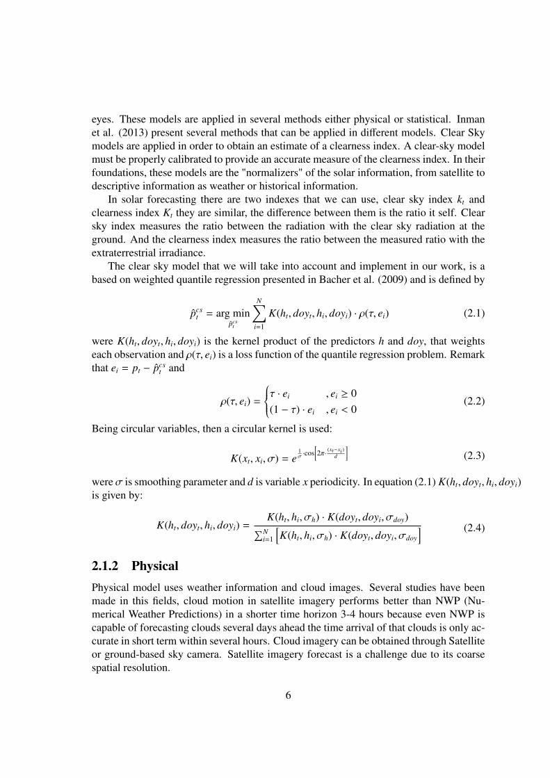
The clear sky model that we will take into account and implement in our work, is abased on weighted quantile regression presented in Bacher et al. (2009) and is defined by

pcst = arg min

pcst

N∑i=1

K(ht, doyt, hi, doyi) · ρ(τ, ei) (2.1)

were K(ht, doyt, hi, doyi) is the kernel product of the predictors h and doy, that weightseach observation and ρ(τ, ei) is a loss function of the quantile regression problem. Remarkthat ei = pt − pcs

t and

ρ(τ, ei) =

τ · ei , ei ≥ 0(1 − τ) · ei , ei < 0

(2.2)

Being circular variables, then a circular kernel is used:

K(xt, xi, σ) = e1σ ·cos

[2π· (xt−xi)

d

](2.3)

wereσ is smoothing parameter and d is variable x periodicity. In equation (2.1) K(ht, doyt, hi, doyi)is given by:

K(ht, doyt, hi, doyi) =K(ht, hi, σh) · K(doyt, doyi, σdoy)∑N

i=1

[K(ht, hi, σh) · K(doyt, doyi, σdoy

] (2.4)

2.1.2 PhysicalPhysical model uses weather information and cloud images. Several studies have beenmade in this fields, cloud motion in satellite imagery performs better than NWP (Nu-merical Weather Predictions) in a shorter time horizon 3-4 hours because even NWP iscapable of forecasting clouds several days ahead the time arrival of that clouds is only ac-curate in short term within several hours. Cloud imagery can be obtained through Satelliteor ground-based sky camera. Satellite imagery forecast is a challenge due to its coarsespatial resolution.

6

Cloud imagery forecast, these images are obtained through satellite or ground-based,are based on Motion vectors to detect and track the motion of the clouds in images. Chowet al. (2011) shown that the use of ground-based total sky imager in forecast cloud up to 10minutes ahead with some limitations, there is the fact that capturing deterministically, ata fine spatial scale, low clouds and large clouds variability is near impossible with NWPand satellites. Besides this, there was also a problem with shadows and obscuration.Jayadevan et al. (2012) produced a similar study recurring to a sun-tracking camera,with higher resolution, compared with an all-sky image, near the sun and the resolutionis independent of time of the day and season. This described an intermittency forecastmethod up to 10 minutes, this study showed that under ideal situation it can provideaccurate forecast 10 minutes ahead within 1 minute.

In physical models, we can also find NWP models, that uses weather information tobuild the model. The basis of this models are the forecast of the atmosphere state, througha set of differential equations that we can see in Lorenz and Heinemann (2012), that de-scribe the physical laws of weather. This kind of models can be categorized in to Globalor Mesoscale Models. Diagne et al. (2013) refer that Global NWP are in operation at15 weather services. Some examples of global NWP are GFS from USA and ECMWF(European Centre for Medium-Range Weather Forecasts). Even with the increasing in theresolution in the last few years, global NWP has a low resolution and it’s impossible toobtain a detailed mapping for a small-scale. In order to perform forecast on this scale, wemight apply a Mesoscale model also referred in the literature as a regional model. As thename of the model indicates, this kind of models covers a region, a part of the Earth, eventhough allow a higher spatial resolution. NWP output can be refined through Postpro-cessing methods, this method could be applied to reduce forecast errors, introduce localeffects, etc. There are several approaches in Postprocessing, the mainstream approachis MOS. Diagne et al. (2013) refer also Kalman filter, Temporal interpolation, Spatialaveraging and Physical post processing approaches.

2.1.3 StatisticalThis type of models are based on historical data, and we can classify as statistical andlearning methods. In learning methods, we find ML algorithms, genetic algorithms, NN,etc. The major studies in this kind of models are focus on the analysis of univariate TimeSeries and more recently ML algorithms. They focus only on the historical informationof each Site.

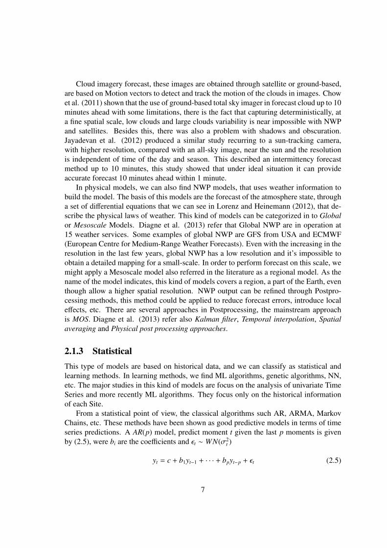
From a statistical point of view, the classical algorithms such AR, ARMA, MarkovChains, etc. These methods have been shown as good predictive models in terms of timeseries predictions. A AR(p) model, predict moment t given the last p moments is givenby (2.5), were bi are the coefficients and εt ∼ WN(σ2

t )

yt = c + b1yt−1 + · · · + bpyt−p + εt (2.5)

7

ARMA is a combination of two models (AR(p) and MA(q)), ARMA(p, q), is a modelwith p autoregressive terms and q moving-average terms, are given by (2.6), were bi arethe AR coefficients, θ j are the MA coefficients and εk ∼ WN(σ2

k)

yt = c + εt +

p∑i=1

biyt−i +

q∑j=1

θiεt− j (2.6)

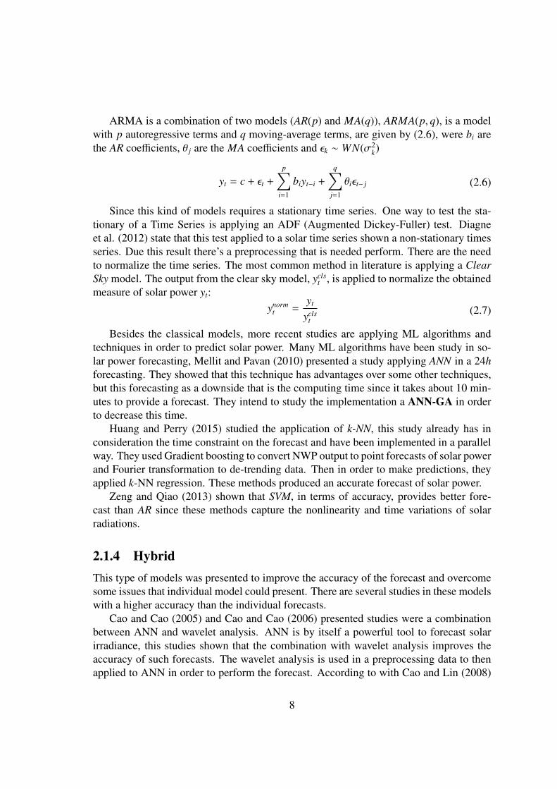
Since this kind of models requires a stationary time series. One way to test the sta-tionary of a Time Series is applying an ADF (Augmented Dickey-Fuller) test. Diagneet al. (2012) state that this test applied to a solar time series shown a non-stationary timesseries. Due this result there’s a preprocessing that is needed perform. There are the needto normalize the time series. The most common method in literature is applying a ClearSky model. The output from the clear sky model, ycls

t , is applied to normalize the obtainedmeasure of solar power yt:

ynormt =

yt

yclst

(2.7)

Besides the classical models, more recent studies are applying ML algorithms andtechniques in order to predict solar power. Many ML algorithms have been study in so-lar power forecasting, Mellit and Pavan (2010) presented a study applying ANN in a 24hforecasting. They showed that this technique has advantages over some other techniques,but this forecasting as a downside that is the computing time since it takes about 10 min-utes to provide a forecast. They intend to study the implementation a ANN-GA in orderto decrease this time.

Huang and Perry (2015) studied the application of k-NN, this study already has inconsideration the time constraint on the forecast and have been implemented in a parallelway. They used Gradient boosting to convert NWP output to point forecasts of solar powerand Fourier transformation to de-trending data. Then in order to make predictions, theyapplied k-NN regression. These methods produced an accurate forecast of solar power.

Zeng and Qiao (2013) shown that SVM, in terms of accuracy, provides better fore-cast than AR since these methods capture the nonlinearity and time variations of solarradiations.

2.1.4 HybridThis type of models was presented to improve the accuracy of the forecast and overcomesome issues that individual model could present. There are several studies in these modelswith a higher accuracy than the individual forecasts.

Cao and Cao (2005) and Cao and Cao (2006) presented studies were a combinationbetween ANN and wavelet analysis. ANN is by itself a powerful tool to forecast solarirradiance, this studies shown that the combination with wavelet analysis improves theaccuracy of such forecasts. The wavelet analysis is used in a preprocessing data to thenapplied to ANN in order to perform the forecast. According to with Cao and Lin (2008)

8

although ANN, in terms of accuracy, performs better than traditional prediction models,ANN-based models are yet reasonable in a forecast precision that researchers and engi-neers are looking for. So in order to address this, they presented a new study to improvethis forecasts. They study the appliance of a dynamic characteristic of a recurrent neuralnetwork (RNN) instead of an ANN, with the ability to catch nonlinearity that wavelet neu-ral network(WNN). They even present a new concept Diagonal recurrent wavelet neuralnetwork (DRWNN) to deal with the fine forecast.

In the same line of study (combining ML algorithms with statistical methods) Ji andChee (2011) presented a Study were its combined ARMA model with time delay neuralnetwork (TDNN). By themselves ARMA a TDNN are very powerful, simulations per-formed in their study show that this hybrid model gives "excellent" results.

In another filing of study Marquez et al. (2013) presented a study that combines aphysical model with a stochastic learning. In this work, the authors use satellite imagesanalysis as input to ANN model. This analysis included velocimetry and cloud index.According to with the authors, this was the first attempt to join stochastic learning withimage processing in order to solar irradiation forecast.

2.1.5 Spatio-temporalAlthough Lorenz et al. (2009) presented a study in physical approach provide by ECMWF,they show that forecast accuracy for an ensemble of a distributed system is higher than theforecast for a single system. This implies that the knowledge of site environment brings abetter forecast performance.

The spatial-temporal models are a "recent" field of study, that take advantage of siteenvironment and from their historical information. This field of study is from statisticalmodels. In this field of study instead of analysing only one site, we are looking to itsneighbours also. Lonij et al. (2012) produced a study where they compare a method usinga Network of residential PV system with an NWP and ground-based camera methods.They have shown that by using a network of PV systems, the physical forecasting methodswere outperformed for a 15-min interval.

Meteorological phenomena have a high geographical auto-correlation, and so the waythat PV systems are formed (centralized or distributed) have an affect over the variabilityand uncertainty. Tabone and Callaway (2015), presented a study where they applied aHMM(hidden Markov model) to predict this characteristics. They intended to deal withthe reserve requirements. They discover that under certain conditions the variability dis-tribution approaches to a Gaussian distribution. They presented the model as a planningtool for additional reserve capacity and\or to balance in a spatial area (large and small)the variability characteristic.

Golestaneha et al. (2015) studied the strong dependency of PV generation uncer-tainty to time and space. To address this situation they had analysed and captured spatio-temporal dependencies in PV generation. They claim that in an operational environmentthat is more sensitive in structure dependence, when space-time correlation is unknown,

9

using probabilistic forecast may provide a suboptimal solution. They verified also thateven when historical data is unavailable in order to find structure dependency of PV gen-erations, an alternative approach might be modelling covariance matrix recursively.

Bessa et al. (2015) applied a VAR framework in order to include the neighbours infor-mation in the forecast. This work applied two different fit methods to VAR framework andused the clear sky model presented by Bacher et al. (2009), based on weighted quantileregression. They showed that NARX (Non-linear Autoregressive with eXogenous inputs)model outperform persistent methods in 15-min and beyond forecasts. They confirmedthat using information of neighbouring improves the forecast accuracy.

Vaz et al. (2016) presented a model for PV prediction with a NN architecture, usinga NARX model, using not only the site meteorological data but also their neighbouringdata. The NARX model presented to be also verify effective in multi-step predictions.

2.2 VARThe vector autoregression (VAR) model were introduced by Sims (1980) and are a exten-sion of Autoregressive (AR) models, to model multivariate time series. The VAR modelhas some descriptive power as well a good forecasting. It often provides a better forecastresult than the AR model. The flexibility of VAR happens because of the conditionalityon potential future paths of the same variable in the model.

An n-variable vector autoregression of order p VAR(p), is a system of n linear equa-tions, on witch every equation describes the dynamics between one variable as a linearfunction of the p previous lags of n variables of the system. A p − th order VAR is:

yt = c + B1yt−1 + B2yt−2 + · · · + Bpyt−p + et (2.8)

or in a matrix notation we have:

Y = BZ + U (2.9)

We can estimate B by applying a classical approach with the OLS. We can also es-timate using the LASSO approach that will lead to a sparser solution and in the samesituation a better result to this estimation.

2.3 `p RegularizationIn Machine Learning and statistics there are some regularization methods, in order toprevent over-fitting of the model to data. In machine learning the most common regular-izations are `1 and `2. Then instead the ML algorithm minimize the lost function f (X),this is regularized by adding is a penalty. This means that the problem is now the mini-mization of new penalized function with `p regularization, f (X) + λ ‖.‖p where λ ≥ 0.

10

`1 regularization are often preferred methods, his main advantage is a sparse modelthat is produced thus performs feature selection within the learning algorithm. There is adrawback in this regularization, `1 is not differentiable, and this might require changes tothe learning algorithms.

2.3.1 LASSOLASSO is an `1 regularization to a linear regression. This method was presented byTibshirani (1994).

In a usual regression situation, where data is in the form :(Xi, yi

), i = 1, ...,N where

Xi =(xi1, ..., xip

)Tare the predictor variables and yi are the responses OLS estimates by

minimizing the residual squared error. There are some techniques to improve this esti-mate, the standard was Subset Selection and Ridge Regression, but both of this techniqueshas some positive aspects and some issues. Subset Selection give a very interpretablemodel but is a very variable technique due to its descriptive nature the feature is retainedor dropped from the model, so with small changes in the data we might select very differ-ent models and so reduce its prediction accuracy. The Ridge Regression is a more stabletechnique because is a continuous process that shrinks coefficients, but this does not setany coefficient to 0 and the models are not so easily interpretable.

Tibshirani (1994) presented a new technique LASSO ( Least Absolute Shrinkage andSelection Operator), this technique combines the best features from Subset Selection andRidge Regression.

Let’s assume that the observations are independent or yi’s are conditionally inde-pendent given xi j’s. Let’s assume also that xi j are standardized so that

∑i

xi j

N = 0 and∑i

x2i j

N = 1. Then LASSO estimate is given by equation (2.10)

(α, β

)= arg min

N∑i=1

yi − α −∑

j

β jxi j

2

s.t. ‖β‖1 ≤ t

(2.10)

were β = (β1, ..., βp)T is the LASSO estimate. To control the shrinkage that is appliedto the estimates its used the parameter t ≥ 0 . For all t, the solution for α is α = y. Withoutlosing generality we can assume that y = 0 and hence omit α, so β is estimate by:

β = arg minN∑

i=1

yi −∑

j

β jxi j

2

s.t. ‖β‖1 ≤ t

(2.11)

The criterion∑N

i=1

(yi −

∑j β jxi j

)2is equal to the following quadratic function:(

β − β0)T

XT X(β − β0

)(2.12)

11

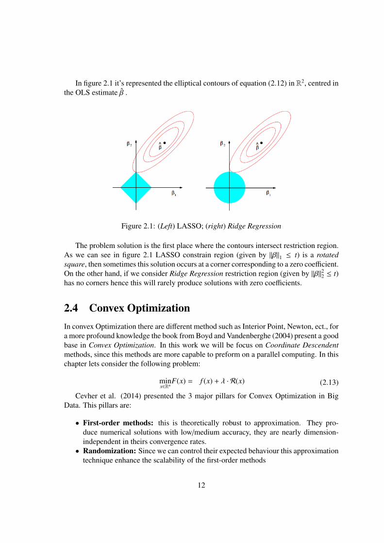
In figure 2.1 it’s represented the elliptical contours of equation (2.12) in R2, centred inthe OLS estimate β .

Figure 2.1: (Left) LASSO; (right) Ridge Regression

The problem solution is the first place where the contours intersect restriction region.As we can see in figure 2.1 LASSO constrain region (given by ‖β‖1 ≤ t) is a rotatedsquare, then sometimes this solution occurs at a corner corresponding to a zero coefficient.On the other hand, if we consider Ridge Regression restriction region (given by ‖β‖22 ≤ t)has no corners hence this will rarely produce solutions with zero coefficients.

2.4 Convex OptimizationIn convex Optimization there are different method such as Interior Point, Newton, ect., fora more profound knowledge the book from Boyd and Vandenberghe (2004) present a goodbase in Convex Optimization. In this work we will be focus on Coordinate Descendentmethods, since this methods are more capable to preform on a parallel computing. In thischapter lets consider the following problem:

minx∈Rn

F(x) = f (x) + λ · R(x) (2.13)

Cevher et al. (2014) presented the 3 major pillars for Convex Optimization in BigData. This pillars are:

• First-order methods: this is theoretically robust to approximation. They pro-duce numerical solutions with low/medium accuracy, they are nearly dimension-independent in theirs convergence rates.

• Randomization: Since we can control their expected behaviour this approximationtechnique enhance the scalability of the first-order methods

12

• Parallel and distributed computation: First-order methods have a flexible frame-work that allows distributing optimization task through parallel computations.

Let’s analyse each one of this pillars. Considering a special case of equation (2.13),where the objective function is a differentiable convex function f F(x) = f (x), the firstorder method applied to this case is the gradient method. This method iteratively updatesx as:

xk+1 = xk − αk∇ f (xk) (2.14)

where k is the counter and αk is the step-size that ensures convergence.When we consider the Composite objective like equation (2.13), where F is com-

posed by a differentiable convex function f and a non-smooth convex function R, thenon-smooth part of the problem could reduce efficiency. The Proximal-gradient methodstake advantage of the composite structure of the problem they retain the convergence rateof the gradient method for the smooth part of the problem. It appears that this is a nat-ural extension of the gradient methods when equation (2.14) is seen as an optimizationproblem:

xk+1 = arg miny∈Rn

{f (xk) + ∇ f (xk)T

(y − xk

) 12αk

∥∥∥y − xk∥∥∥2

2

}(2.15)

Considering now the problem as an all, we can define the proximal by simply include thenon-smooth part of the problem:

xk+1 = arg miny∈Rn

{f (xk) + ∇ f (xk)T

(y − xk

) 12αk

∥∥∥y − xk∥∥∥2

2+ g(y)

}(2.16)

So the update rule of the proximal-gradient method is given by equation (2.16) or in areduced form:

xk+1 = proxαkg

(xk − αk∇ f (xk)

)(2.17)

In theory, the first-order methods are good methods for very large-scale problems,but in practice, the exact numerical computations iterations demanded by them can makethese simple methods infeasible, as the dimensions of problems grow. Hence these meth-ods as very robust using approximations of their optimization primitives Schmidt et al.(2011),

2.5 Convex Optimization AlgorithmsCoordinate Descent method, are based on the concept that the minimization of a mul-tivariate function G(X) can be achieved by solving univariate (or a simplest problem)optimization problem in a loop. Figure 2.2 represent this idea.

13

Figure 2.2: Coordinate Descent

In this section, we will study some algorithms that try to deal with the problem givenby (2.13) in a parallel manner. In the end of the chapter will be presented a summary ofthe algorithms in table 2.1. For each one of this algorithms, we will consider the baseproblem given by (2.13) and present some restrictions and conditions to the algorithm.The base algorithm is RCDM, that present the first study of random select the coordinateto update.

Random Coordinate Descent Method (RCDM)

In Nesterov (2010) was presented RCDM, for problems where the regularization functionis zero, R(x) = 0. He define the optimal coordinate step as

Ti(x)de f .= x −

1Li

Ui∇i f (x)# (2.18)

It was also define a random counter Rα, that generate integer value i ∈ 1, · · · , n with aprobability:

p(i)α = Lαi

n∑j=1

Lαj

−1

(2.19)

So any operation k = Rα means that k is an integer value from 1, · · · , n is chosen with aprobability define in equation (2.19). A Special case is when α = 0 then R0 generates auniform distribution. Knowing step-size and the probability of choice we can define themethod:

Algorithm 1 Random Coordinate Descent Method1: choose x0 ∈ R

n and α ∈ R2: f or k ≥ 03: choose ik = Rα4: update xk+1 = Tik(xk)

14

Shotgun

In Bradley et al. (2011) was presented the algorithm Shotgun, this algorithm was basedon Stochastic Coordinate Descent (SCD) from Shalev-Shwartz and Tewari (2009). Thisstudy was for `1 regularization function, R(x) = ‖x‖1. The main idea in this algorithmis applying the coordinate update not only for one but P coordinates uniformly selected,where P is the number of processors in the machine. The algorithm 2 we can see eachone of the steps where δx j indicates the update that is perform in coordinate j

Algorithm 2 Shotgun1: choose P ≥ 1, the number of parallel updates2: choose x0 ∈ R

2d+

3: while not converge do (In parallel on P processors)4: choose j ∈ {1, · · · , 2d} uniformly at random5: set δx j ← max

{−x j,

−(∇F(x)) j

β

}6: update x j ← x j + δx j

7: end while

This algorithm was applied to LASSO and its performance was measure against othersLASSO solvers. Shotgun performs well and the converging rate is faster then others,particularly in Large sparse datasets were most algorithms fail.

GRock

Let’s consider that R(x) is separable and R(x) =∑n

i=1 r(xi). Let’s consider also that f (X) =

L(Ax, b) and for simplicity L is convex and A has columns with unit `2-norm. Let β > 0such that:

L(A(x + d), b) ≤ L(Ax, b) + gT d +β

2d2

where g = AT∇L(Ax, b), qe can define to each coordinate i it’s potential:

di = arg mindλ · r(xi + d) + gid +

β

2d2 (2.20)

where gi is the ith entry of g. We can express equation (2.20) in it’s closed form di =

prox λβ r

(xi −

1βgi

)− xi. This algorithm considers the division of coordinates into N blocks,

and for each j block:

m j = max{|d| : d is an element of d j

}(2.21)

GRock updates the best coordinate of the best P blocks. Let s j such that m j = ds j , thismeans that s j achieves it’s maximum.

This algorithm is not parallel in terms of computing, but the paper gives the way ofparallelization of the algorithm steps 3 and 4 can be made in parallel and then step 5 couldbe executed through MPI and finally step 6 can be preformed in parallel also.

15

Algorithm 3 GRock1: Initialize x = 0 ∈ Rn

2: while not converge do3: d j ← (2.20), for each block j4: m j, s j ← (2.21), for each block j5: P ← the indices of P blocks with largest m j

6: xs j ← xs j + ds j , for each j ∈ P7: end while

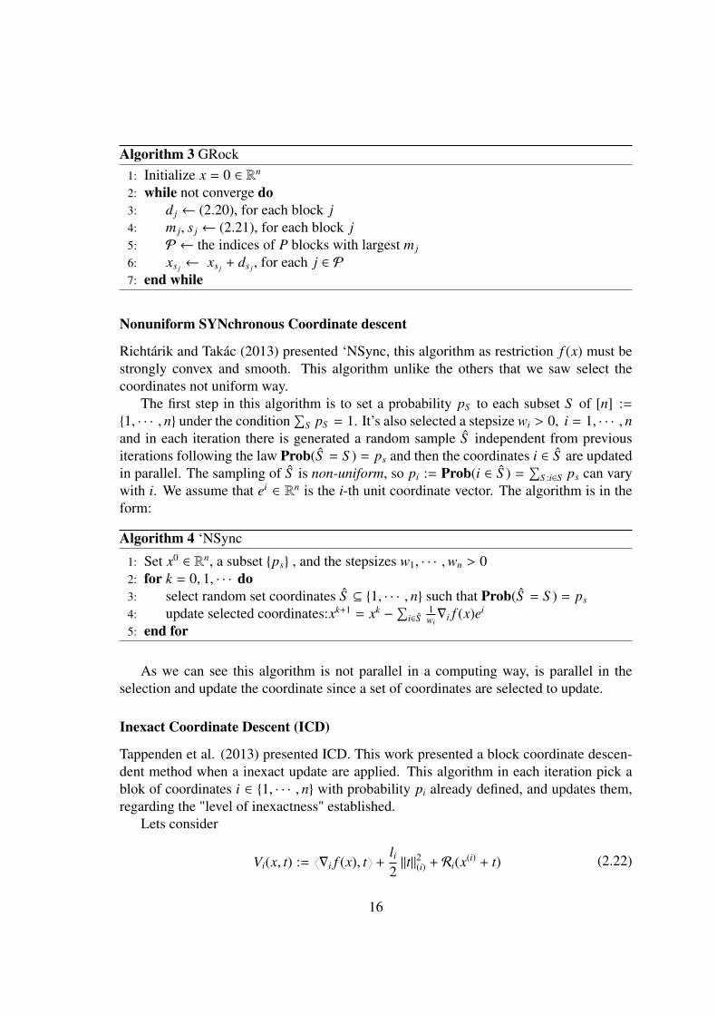
Nonuniform SYNchronous Coordinate descent

Richtárik and Takác (2013) presented ‘NSync, this algorithm as restriction f (x) must bestrongly convex and smooth. This algorithm unlike the others that we saw select thecoordinates not uniform way.

The first step in this algorithm is to set a probability pS to each subset S of [n] :={1, · · · , n} under the condition

∑S pS = 1. It’s also selected a stepsize wi > 0, i = 1, · · · , n

and in each iteration there is generated a random sample S independent from previousiterations following the law Prob(S = S ) = ps and then the coordinates i ∈ S are updatedin parallel. The sampling of S is non-uniform, so pi := Prob(i ∈ S ) =

∑S :i∈S ps can vary

with i. We assume that ei ∈ Rn is the i-th unit coordinate vector. The algorithm is in theform:

Algorithm 4 ‘NSync

1: Set x0 ∈ Rn, a subset {ps} , and the stepsizes w1, · · · ,wn > 02: for k = 0, 1, · · · do3: select random set coordinates S ⊆ {1, · · · , n} such that Prob(S = S ) = ps

4: update selected coordinates:xk+1 = xk −∑

i∈S1wi∇i f (x)ei

5: end for

As we can see this algorithm is not parallel in a computing way, is parallel in theselection and update the coordinate since a set of coordinates are selected to update.

Inexact Coordinate Descent (ICD)

Tappenden et al. (2013) presented ICD. This work presented a block coordinate descen-dent method when a inexact update are applied. This algorithm in each iteration pick ablok of coordinates i ∈ {1, · · · , n} with probability pi already defined, and updates them,regarding the "level of inexactness" established.

Lets consider

Vi(x, t) := ∇i f (x), t +li

2‖t‖2(i) + Ri(x(i) + t) (2.22)

16

This algorithm best applies to situations where is easier to approximately minimizet → Vi(x, t) than either to approximately minimize t → F(x+Uit) and/or exactly minimizet → Vi(x, t).

In some cases calculate exact update is impossible, or is computational complex andinfeasible in terms of time of execution. The propose of this algorithm was to allow inex-actness in update step, in this way allowing a higher range of problems were CoordinateDescendent could be applied.

Semi-Stochastic Coordinate Descent (S2CD)

Konecný et al. (2014) presented this algorithm. In this work, the authors consider thestrongly convexity of F and considered that is the average of multiple strongly convexfunctions. The algorithm is split into two different steps that are in a loop. First, theystarted with a deterministic calculation of the gradient followed by a stochastic step, thisstep is the point of divergence from other algorithms in the literature. In this step, the al-gorithm selects a function fi and a coordinate j at random using nonuniform distributionsand update a single coordinate. This is not a parallel algorithm since it only updates asingle coordinate by iteration. The algorithm itself is represented as follows:

Algorithm 5 S2CDSet m (max # of stochastic steps per epoch),h > 0 (stepsize parameter); x0 ∈ R

n (startingpoint)for k = 0, 1, · · · do

compute and store ∇ f (xk) = 1n

∑i ∇ fi(x)

initialize inner loop: yk,0 ← xk

Let tk = T ∈ {1, · · · , n} with probability (1−µh)m−T

β

for t = 0 to tk − 1 doPick coordinate j ∈ {1, · · · , n}Pick function index i from the set

{i : Li j > 0

}with probability qi j

Update the jth coordinate:yk,t+1 ← yk,t − hp−1

j

(∇ j f (xk) + 1

nqi j

(∇ j fi(yk,t) − ∇ j fi(xk)

))e j

end forReset the starting point: xk+1 ← yk,tk

end for

Accelerated Parallel Proximal Coordinate Descent Method (APPROX)

This algorithm was presented by Fercoq and Richtárik (2013) and the proposed methodis simultaneously Accelerated, Parallel and Proximal. This method was proposed forminimizing a sum of convex functions, where each one of them depends on a small set

17

of coordinates. This method is more capable to obtain a high-accuracy solution in non-strongly convex problems since it’s accelerate, can take advantage of parallel computingdue to its parallel nature, has a faster convergence rate since longer stepsizes are proposedand there is no need to perform full-dimensional vector operations. The stepsize proposedin this work is based on ESO, this framework was presented in Qu and Richtárik (2014b),in this work a new model of ESO was presented.

Algorithm 6 APPROX

1: Choose x0 ∈ RN and set z0 = x0 and θ0 = τ

n2: for k ≥ 0 do3: yk = (1 − θk) xk + θkzk

4: Generate a random set of blocks S k ∼ S5: Zk+1 = zk

6: for i ∈ S k do7: Z(i)

k+1 = arg minz∈RNi

{∇i f (yk), z − y(i)

k + nθkvi2τ

∥∥∥z − z(i)k

∥∥∥2

(i)+ ψi(z)

}8: end for9: xk+1 = yk + n

τθk (zk+1 − zk)

10: θk+1 =

√θ4

k +4θ2k−θ

2k

211: end for

ALPHA

Qu and Richtárik (2014a) proposed this method based on arbitrary sampling, that is aconcept not yet studied in the previous literature. Basically, this method at each iterationselects a subset of coordinates at random, following an arbitrary distribution. This methodis extraordinarily flexible since the authors proposed a general randomized Coordinatedescendent method, that could be implemented in a serial or parallel way, with or withoutarbitrary sampling. They focused on non-strongly convex function study, and they referthat further studies must be performed in order to set a unified algorithm and complexityanalysis for strongly and non-strongly convex functions.

18

Algorithm 7 ALPHA

1: Parameters: proper sampling S with probability vector p = (p1, · · · , pn),v ∈ Rn++,

sequence {θk}k≥0

2: Initialization: choose x0 ∈ domψ and set z0 = x0

3: for k ≥ 0 do4: yk = (1 − θk) xk + θkzk

5: Generate a random set of blocks S k ∼ S6: Zk+1 ← zk

7: for i ∈ S k do8: Zi

k+1 = arg minz∈RNi

{∇i f (yk), z + θkvi

2pi

∥∥∥z − zik

∥∥∥2

i+ ψi(z)

}9: end for

10: xk+1 = yk + θk p−1 · (zk+1 − zk)11: end for

Hydra2

Hydra2 was presented by Fercoq et al. (2014), this algorithm is an specialization of AP-PROX method with a distributed setting or an accelerate version of Hydra algorithmproposed by Richtárik and Takác (2012). This algorithm conceptually was based on acomputer network, and within each one of this computers, we take advantage in parallelcomputing recurring to each one of its cores. They also proposed a new stepsize parame-ters in order that Dii satisfy ESO assumption. In their experiments, they showed that thenew easily computable stepsize achieves a comparable convergence speed with respect toothers. As we can see in the algorithm he can easily set this as a parallel algorithm bysimple consider that ou computer network only has 1 machine. They also showed thateven though the cost per iteration, in runtime, is higher in Hydra2, than in Hydra, Hydra2

converges faster than Hydra. The algorithm is represented as follows:

19

Algorithm 8 Hydra2

1: Set {Pl}cl=1, 1 ≤ τs,{Dii}

dii=1,z0 ∈ R

d

2: Set θ0 = τs and u0 = 0

3: for k ≥ 0 do4: zk+1 ← zk, uk+1 ← uk

5: for each computer l ∈ {1, · · · , c}in parallel do6: pick a random set of coordinates S l ⊆ Pl,

∣∣∣S l

∣∣∣ = τ

7: for each i ∈ S lin parallel do8: ti

k = arg mint

f′

i (θ2kuk + zk)t + sθkDii

2τ t2 + Ri(zik + t)

9: zk+1 ← zik + ti

k, uik ← ui

k −

(1θ2

k− s

τθk

)tik

10: end for11: end for12: θk+1 = 1

2

(√θ4

k + 4θ2k − θ

2k

)13: end for

Output:θ2kuk+1 + zk+1

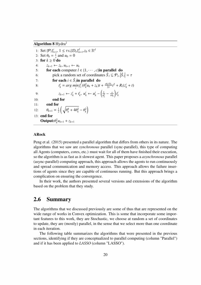
ARock

Peng et al. (2015) presented a parallel algorithm that differs from others in its nature. Thealgorithms that we saw are synchronous parallel (sync-parallel), this type of computingall Agents (computers, cores, etc.) must wait for all of them have finished their execution,so the algorithm is as fast as it slowest agent. This paper proposes a asynchronous parallel(async-parallel) computing approach, this approach allows the agents to run continuouslyand spread communication and memory access. This approach allows the failure inser-tions of agents since they are capable of continuous running. But this approach brings acomplication on ensuring the convergence.

In their work, the authors presented several versions and extensions of the algorithmbased on the problem that they study.

2.6 SummaryThe algorithms that we discussed previously are some of thus that are represented on thewide range of works in Convex optimization. This is some that incorporate some impor-tant features to this work, they are Stochastic, we choose at random a set of coordinatesto update, they are (mostly) parallel, in the sense that we select more than one coordinatein each iteration.

The following table summarizes the algorithms that were presented in the previoussections, identifying if they are conceptualized to parallel computing (column "Parallel")and if it has been applied to LASSO (column "LASSO").

20

Name Paper Parallel LASSORCDM Nesterov (2010)Shotgun Bradley et al. (2011) X XGRock Peng et al. (2013) X X‘NSync Richtárik and Takác (2013)

APPROX Fercoq and Richtárik (2013) X XICD Tappenden et al. (2013)

S2CD Konecný et al. (2014)APLHA Qu and Richtárik (2014a)Hydra2 Fercoq et al. (2014) X XARock Peng et al. (2015) X X

Table 2.1: Algorithms in Literature

21

Chapter 3

Contributions to LASSO-VAR ModelFitting

This work intends to give an LASSO approach to the estimation of the coefficient matrix,B, of the VAR problem (2.9). This approach is commonly addressed as the LASSO-VAR,This problem can be described as the following expression:

minB

12‖Y − BZ‖2F + λ ‖B‖1 (3.1)

To find an estimation B for the coefficient matrix B we will apply the algorithmsShotGun and GRock described in the former chapters. Both algorithms will be appliedwith the traditional sequential programming techniques and by using parallel computerprogramming techniques when these are possible.

Besides aforementioned changes, it terms of the LASSO-VAR problem it was alsotaken into consideration some assumptions. Considering a VARk(p) problem, then a pth-order can be expressed as:

Yt = 3 +

p∑l=1

BlYt−l + ut (3.2)

where Yt, 3, ut ∈ Rk each Bl represents a coefficient matrix k×k. We can translate equation

(3.2) to a matrix notation asY = 31

′

+ BZ + U (3.3)

Where 1 denotes the vectors of ones, with dimension T × 1, and 3 the intercept vectorWe intend to estimate B applying LASSO strategy, so by extending Tibshirani (1994) weget the following objective function:

12

∥∥∥Y − 31′

− BZ∥∥∥2

F+ λ ‖B‖1 (3.4)

In order to simplifying computation we might consider the centred form, so equation

22

(3.4) becomes12‖Y − BZ‖2F + λ ‖B‖1 (3.5)

where Y = Y − Y and Z = Z − ZSo with all of this in consideration we can establish that the 3 Intercept term can be

expressed by the following equation:

3 = Y + BZ (3.6)

We already know that LASSO is given by F(B) = G(B) + λR(B), where R(B) is notdifferentiable we must consider sub-gradient of F(B), so:

∇F(B) = ∇G(B) + ψ(R(B)) (3.7)

where

ψ(R(B)) ∈

{sgn(R(B))} ,R(B) , 0[−1, 1] ,R(B) = 0

(3.8)

3.1 AlgorithmsAs presented in Bradley et al. (2011) and Peng et al. (2013), the algorithms were studiedto a vector lasso estimation. In the article they solved lasso estimation x for the problem:

minx

12‖y − Ax‖22 + λ ‖x‖1 (3.9)

Our problem is the estimation of the matrix B, so we need to tweak a little the algo-rithms to be able to apply them to the Lasso-VAR problem.

There were no majors changes to the algorithms, these changes were in the selectioncriteria as well to the gradients. Both algorithms stands under the assumptions of ConvexOptimization algorithms for problems:

min F(B) = G(B) + λR(B) (3.10)

were G is differentiable and R is separable. So as we can see in equation (3.1) we candescribe G(B) = 1

2 ‖Y − BZ‖2F and R(B) = ‖B‖1, then both algorithms will use the gradientof G(B) that is ∇G(B) = −(Y − BZ)ZT . Taking all this in consideration both algorithmswill aplly a Soft-Threshold to the update, we will consider the generic equation for thissoft-threshold as:

ST λ,ρ(x) = sign(x)max{|x| − λρ, 0} (3.11)

23

Besides the programming paradigm, we will also see this as a single problem aswell as sub-problems. This means that we will apply both algorithms and programmingparadigms to the problem (3.1) as well to each sub-problem to each location, solving allthe 44 sub-problems of estimation B by estimate each line as a single problem.

3.1.1 ShotgunThis algorithm is described in algorithm 2, as discussed above this algorithm will bechanged as explained in the following sub-sections.

But before we address the algorithm changes lets take a look at the step-size conditionfor this algorithm. As is mentioned in Bradley et al. (2011), the convergence is directlyrelated to the step-size update. This step-size assures the algorithm convergence, butthis is a throwback since that for a better convergence implies a higher runtime of thealgorithm, this means that for a better solution the model training time is higher. Forthis work, we used the step-size proposed in Nicholson et al. (2014). In this article, theauthors proposed a step-size given by :

ρ =1λmax

(3.12)

Where λmax is the higher eigenvalue of ZZT . This operation as also a considerableruntime and therefore increase the model training.

Sub-Problems

To this approach we need to consider the algorithm 2. The main difference in this ap-proach is a new cycle in order to run it for all sub-problems an in the computation of thegradient. To the sub-problem approach the gradient is given by:

∇ f (b) = −ZT (y − Zb) (3.13)

Where y represents the current sub-problem i, y = Y(i) and b represents the line fromB that we intend to estimate in each sub-problem. So the algorithm that was applied is:

24

Algorithm 9 Shotgun Sub-problems1: choose P ≥ 1, the number of parallel updates2: Set B = 0k×kp , ε and λ3: for each j ∈ {1, · · · , k} do4: b← B[ j, ] = 01×kp

5: y← Y[ j, ]6: while threshold>ε do7: bold ← b8: Choose P positions uniformly at random r ∈ {1, · · · , k},9: Compute g j,r := ∇ f (bold)r

10: Update br ← ST λρ(boldr − ρgr)

11: update threshold12: end while13: end for14: compute (3.6) to estimate 3

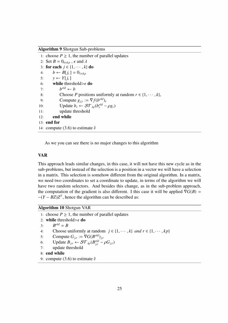
As we you can see there is no major changes to this algorithm

VAR

This approach leads similar changes, in this case, it will not have this new cycle as in thesub-problems, but instead of the selection is a position in a vector we will have a selectionin a matrix. This selection is somehow different from the original algorithm. In a matrix,we need two coordinates to set a coordinate to update, in terms of the algorithm we willhave two random selectors. And besides this change, as in the sub-problem approach,the computation of the gradient is also different. I this case it will be applied ∇G(B) =

−(Y − BZ)ZT , hence the algorithm can be described as:

Algorithm 10 Shotgun VAR1: choose P ≥ 1, the number of parallel updates2: while threshold>ε do3: Bold = B4: Choose uniformly at random j ∈ {1, · · · , k} and r ∈ {1, · · · , kp}5: Compute G j,r := ∇G(Bold) j,r

6: Update B j,r ← ST λρ(Boldj,r − ρG j,r)

7: update threshold8: end while9: compute (3.6) to estimate 3

25

3.1.2 GRockAs presented in Peng et al. (2013), this algorithm stands under the condition that matrixZ has a 2−norm column value, this will be the main condition to determinate the updatedmerit as described in the algorithm 3 (the original algorithm presented on Peng et al.(2013)). In this algorithm, only the P coordinates with higher merit will be chosen to beupdated. Equations (2.20) and (2.21) described the merit as well the update selection oforiginal algorithm. In this work, this assumptions remain valid, but the merit calculationwill be slightly different. The merit will use the 2−norm assumption and use this 2−normcolumn values to determinate the merit of each update.

The process to determinate the updated merit will be described next, first, let’s con-sider

Z2−norm =

[ ∥∥∥Z[1]

∥∥∥2

2

∥∥∥Z[2]

∥∥∥2

2

∥∥∥Z[3]

∥∥∥2

2· · ·

∥∥∥Z[kp]

∥∥∥2

2

](3.14)

the vector that represents the 2− norm column of Z. After this vector is calculated wecan consider the β to being:

β = B −∇G(B)Z2−norm

(3.15)

After the β value is determinate we can apply a soft-threshold to it, being this given byequation (3.16)

βthreshold = sign(β)max{|β| −

λ

Z2−norm, 0

}(3.16)

Then we consider d matrix as:

d = βthreshold − β (3.17)

This d matrix is the matrix used to determinate the P updates with higher merit, there-fore select to update.

With all this in consideration, we can now take a look at the changes of the algorithm,the aforementioned process to merit calculation is the major adaptation to the algorithm.

Sub-Problems

Since we are looking at each problem separately, the obvious change, just like in Shotgunalgorithm, is the additional cycle to run each one of the locations. The merit calculationwas already described. So the applied algorithm can be described as:

26

Algorithm 11 GRock Sub-problems1: choose P ≥ 1, the number of parallel updates2: Set B = 0k×kp , ε and λ3: compute Z2−norm, as described in (3.14)4: for each j ∈ {1, · · · , k} do5: b← B[ j, ] = 01×kp

6: y← Y[ j, ]7: while threshold>ε do8: bold ← b9: compute β, as described in (3.15)

10: compute d, as described in (3.17)11: Select P coordinates with higher update merit.12: update b j ← b j + d j13: update threshold14: end while15: end for16: compute (3.6) to estimate 3

VAR

For this approach, there is no major besides of the merit calculation. After it is onlythe position of those in the matrix that is calculated to be updated. So the algorithm isquite similar to the previous minus the obvious cycle to run each sub-problem. Hence thealgorithm is:

Algorithm 12 GRock Sub-problems1: choose P ≥ 1, the number of parallel updates2: Set B = 0k×kp , ε and λ3: compute Z2−norm, as described in (3.14)4: while threshold>ε do5: compute β, as described in (3.15)6: compute d, as described in (3.17)7: Select P coordinates with higher update merit.8: update B j,r ← B j,r + d j,r

9: update threshold10: end while11: compute (3.6) to estimate 3

27

3.2 SummaryLet’s recap, just a few concepts that we saw till now. In this work, we will consider 2 majorapproaches to the problem, consider the problem as a whole and apply LASSO-VAR toestimate the coefficient matrix B. And another approach that is splitting the problem toeach one of the location, meaning that it will estimate for each location is the respectivecoefficient line.

Besides the approaches to the problem, we will also consider two different approachesin terms of computer programming paradigms. In terms of computer programming, it willconsider the traditional sequential paradigm and also the parallel paradigm. In terms ofalgorithms that were presented the only change that is made is the P value, that in thesequential paradigm it will be 1, meaning that at each iteration only 1 update will beperformed.

28

Chapter 4

Case Study

This chapter aims to present and analyse some results from the trained models. This re-sults will be compared to the results obtained in Trindade (2014). In that work, the authorapplied an OLS estimator for B. In this chapter, it will be presented the forecast mod-els’error so that we can make a comparison in terms of their error and will be presented,as well, some forecasts for these models.

This chapter will be divided into two major sections according to the problem ap-proach, Sub-problem and VAR, to the algorithms. In each of this section, the aforemen-tioned process of error and forecast presentation will be applied.

But first, let’s take a look at the used data for training and to test all models.

4.1 DataThis section aims to explain the used data to train and test the models of prediction, forthe problem (3.1). The PV production is highly seasonal, the PV production is higher inthe summer than it is in winter. Besides this seasonality of the seasons, this productionis also dependent on the period of the day. On figure 4.1 we can see the difference inmonthly production between winter month and summer month and in the figure 4.2 wecan see the difference in daily production between winter day and summer day. We cansee in 4.1 the behaviour of PV production in different months and seasons, in 4.1a wehave PV production in a Winter time and on 4.1b we have the production on Summer. In4.2 is represented a daily production on this months. As we can observe there are periodswhere there is no production, and that this is also affected by the season as expected sincethe solar exposition is larger at summer than at the winter.

29

(a) February of 2011 (b) June of 2012

Figure 4.1: Monthly Production

(a) February 1st, 2011 (b) June 30th 2012

Figure 4.2: Monthly Production

The used data to train and test all models are referent to 44 one − hour time stepsEB. Those EB’s are part of 60 different one − hour time step and represents a 1500km2

SMART Grid. Each one of those EB’s is represented by 1082 observations made betweenFebruary 1st, 2011 and March 6th, 2013. In a PV production, there is a time frame wherethere is no production made, this time frame is between 20 p.m. and 6 a.m. Due to thislack of production and since the models considers pt and pt−1 as an input variable, thetime frame for predictions are restricted depending on the time step. For example forone − hour − ahead it is only possible to forecast for the period 9 a.m. to 19 p.m., andfor 6 − hour − ahead forecast the time frame for that forecasting is 14.pm to 19 p.m. Therecord values were normalised using the Clear Sky Model that was explained on section2.1. The Clear Sky Model is given by:

pnormt =

pt

pcst

(4.1)

On Trindade (2014) it was applied two different persistent models, those models in-stead of consider the prediction the record values they consider the forecast result fromatwo− step process, This means that it take pnorm

t or pnormt−24+k as the normalised forecast val-

ues. Consider the models persistent(τ) being pnormt+k = pnorm

t and the model persistent(τ24)as being pnorm

t+k = pnormt−24+k. Then the forecast value is given by:

30

pt+k = pnormt+k pcs

t+k (4.2)

In this Work the clear sky parameters that was identified in Trindade (2014) τ = 0.85and for 3 we consider 3 = 0.01.

In the same work, the author presents the normalised methods to evaluate the models.The Root Mean Square is given by equation (4.3).

nRMS Ek =

1N

√∑Nt=1(pt+k − pt+k)2

max(pt+k)(4.3)

To understand the model bias it is necessary the normalization of the bias as in equa-tion (4.4).

nBias =

1N

∑Nt=1(pt+k − pt+k)2

max(pt+k)(4.4)

As already described, in this work we intend to estimate B of the Lasso-VAR problemof equation (3.1). This issue will be addressed by two different programming paradigms,the traditional sequential method and in a parallel paradigm. First, lets take a look at thealgorithms and the adaptations made in this work.

4.2 Sub-problemIn this sections, we will analyse the models obtained from the sub-problem approach tothe problem. It will be presented for both algorithms.

4.2.1 RMSEFigures 4.3 and B.1 represent the RMSE for step t + 1 for the parallel and sequential ap-proach respectively. As we can see, the sequential technique does not bring any advantageand in terms of forecast error the Shotgun models are very similar to the OLS model, butthe runtime for these models train is very expensive, so there is no gain in consideringthese models. In the other hand, the Shotgun parallel models are quite a bit better andthe error of those models is lower than the OLS model error, even in the outlier stationsthe error is considerably lower than the OLS model. All models present similar errors buttaking an overall look at those errors, model λ = 0 is lower error rate on ≈ 43% stations.

The greater gain in these Shotgun models is not for step t + 1 but for the next steps. Ifwe look at figure 4.4 we can see that the OLS model presents a significantly higher errorthan the Shotgun models. In these cases, even the sequential approach performs better

31

Figure 4.3: Shotgun (sub-problem) parallel models RMSE for t + 1

than the OLS model, even though they are worst than the parallel methods as we can seein the figure B.2 and the runtime is higher, so there is no gain in considering these models.

32

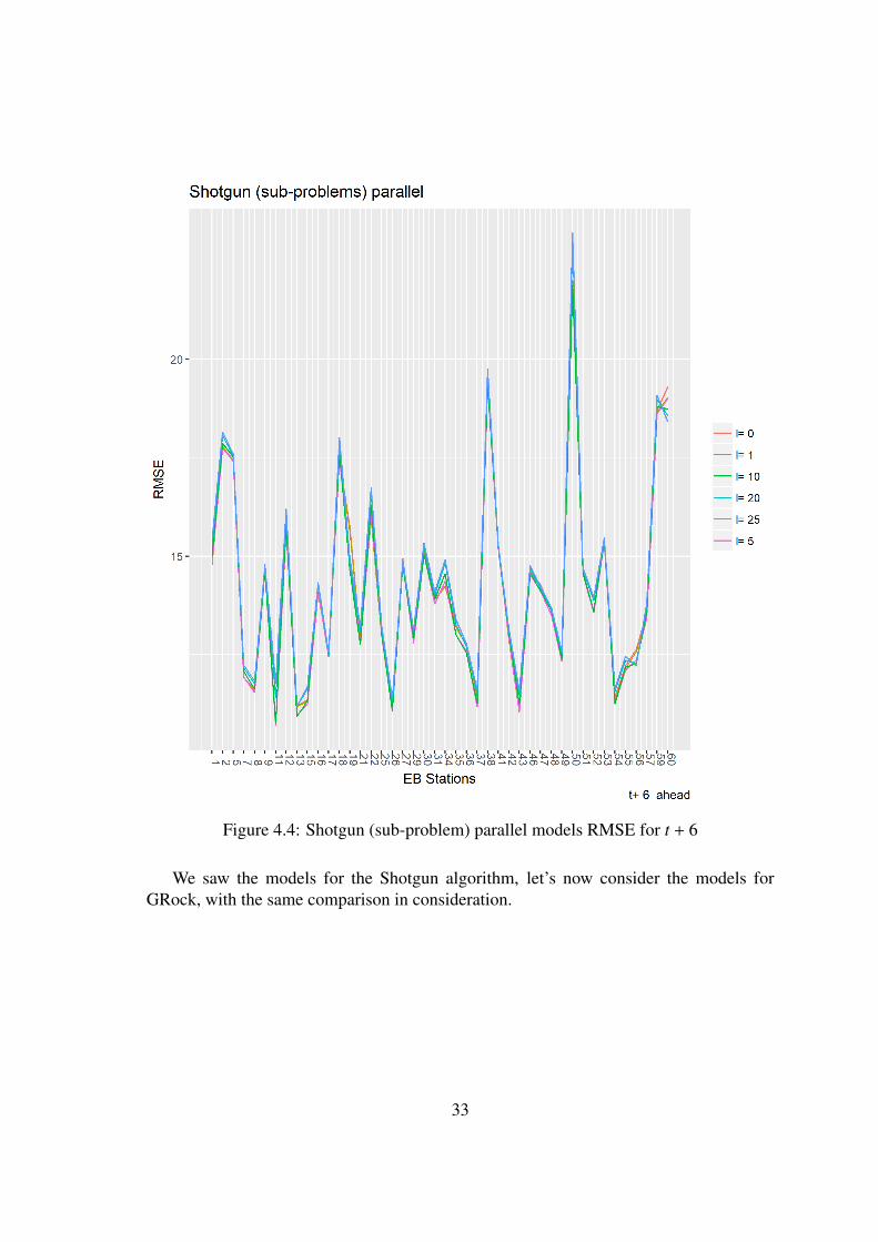
Figure 4.4: Shotgun (sub-problem) parallel models RMSE for t + 6

We saw the models for the Shotgun algorithm, let’s now consider the models forGRock, with the same comparison in consideration.

33

We can see on figure 4.5 that the GRock model error is quite similar to the errorobtained by the OLS model. In figure B.3 it is presented the performance obtained by thesequential methods and as we can see the performance of these models is quite worst, sothe sequential method models are not one to consider.

Figure 4.5: GRock (sub-problem) parallel models RMSE for t + 1

34

Figure 4.6: GRock (sub-problem) parallel models RMSE for t + 6

Unlike the Shotgun models, the GRock Models has no greater gain in the further steps,in figure 4.6 we can see that there are some stations where the error is lower by the GRockmodels and in the others the OLS is quite similar to the GRock models, but the differenceis not significant. The same happens on the sequential methods that we can see on figureB.4. These results are quite better than the parallel methods, yet the difference is notenough to consider them.

35

4.2.2 ForecastIn this section we will take a look at the model’s forecast, taking in consideration thesame principal consideration of comparison with the OLS model. We will see some sea-sons’forecast (Spring, Summer, Autumn, and winter) to see the models’adaptation thedifferent clouds formation as well as the time frame available for the forecast.

Figure 4.7: EB17 Shotgun (sub-problem) parallel models’step t + 1 forecast for 2012-06

As we can see on figure 4.7, the OLS model over-forecast in the major cases, meaningthat the forecasts of this models usually is higher than the observed leading to an expec-tation that after will not correspond. Shotgun models are under-forecast those values,meaning that usually, these models are forecasting below the observed values.

As we can see on figure 4.8 the Shotgun models are better fit to the observed values,when compared with the OLS model. We can see that these models are more similar tothe observed values than the OLS model. Considering figure 4.2b we can see that June30th 2012 as a cloudy day and the PV production ha some kind of "interruption", so letsconsider the period 2012-06-28 until 2012-07-02. As we can see on figure 4.9 the shotgunmodels are quite fit to the observed values, on June 30th the models does not fit as in theremain days, particularly between 12:00-15:00, at 15:00 the model and the observed arequite similar but after 15:00 the models starts do deviate again.

For step t + 6 these fit between shotgun models and observed values is also verified,yet for the cloudy day June 30th this fit is not verified as it was somehow in step t + 1.

If we consider now the GRock models, we can see on figure 4.11 that these models

36

Figure 4.8: EB17 Shotgun (sub-problem) parallel models’step t + 6 forecast for 2012-06

Figure 4.9: EB18 Shotgun (sub-problem) parallel models’step t + 1 forecast for period2012-06-28/2012-07-02

are quite similar to the OLS models when considering step t + 1, but when consideringstep t + 6 start to deviate from it as we can see on figure 4.12.

37

Figure 4.10: EB18 Shotgun (sub-problem) parallel models’step t + 6 forecast for period2012-06-28/012-07-02

If we zoom in into the first 3 days (2012-02-02 until 2012-02-04) then we can seethe that the GRock performs a little bit better than the OLS model. If we look at figure4.13 we see that the models are very similar. A positive point of these models is that thetrajectories of the forecast are very similar to the trajectories of the observed values, thisfeature is quite interesting. In figure 4.14 we can see that the GRock models are verydeviated from the real value as well from the OLS model.

38

Figure 4.11: EB51 GRock (sub-problem) parallel models’step t + 1 forecast for 2012-02

Figure 4.12: EB51 GRock (sub-problem) parallel models’step t + 6 forecast for 2012-02

39

Figure 4.13: EB51 GRock (sub-problem) parallel models’step t + 1 forecast for period2012-02-02/012-02-04

Figure 4.14: EB51 GRock (sub-problem) parallel models’step t + 6 forecast for period2012-02-01/012-02-03

40

4.3 VARLet’s now take a look at the problem approach, where the problem is considered as awhole.

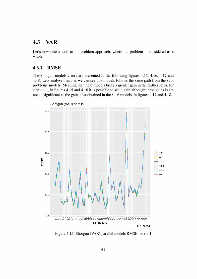
4.3.1 RMSEThe Shotgun models’errors are presented in the following figures 4.15, 4.16, 4.17 and4.18. Lets analyse them, as we can see this models follows the same path from the sub-problems’models. Meaning that these models bring a greater gain in the further steps, forstep t + 1, in figures 4.15 and 4.16 it is possible to see a gain although these gains is arenot so significant as the gains that obtained in the t + 6 models, in figures 4.17 and 4.18.

Figure 4.15: Shotgun (VAR) parallel models RMSE for t + 1

41

Figure 4.16: Shotgun (VAR) sequential models RMSE for t + 1

42

Figure 4.17: Shotgun (VAR) parallel models RMSE for t + 6

43

Figure 4.18: Shotgun (VAR) sequential models RMSE for t + 6

If we compare the models for step t + 6 figures 4.17 and 4.18 we observe a differencethat was not observed in the sub-problem approach, the sequential method performs alittle better than the parallel method, this particular case will be discussed in sections 5.1and 5.2.

The Shotgun models’performances were discussed, lets now take a look to the GRockmodels. Figures 4.19, 4.20, 4.21 and 4.22 shows the error obtained by the GRock models.The figures 4.19 and 4.20 are representative of the models for t + 1 step and we can seethese models does not present any gain, preforming way worst than the OLS model, andthe scenario is worst as the forecast step goes further as we can see in figures 4.21 and

44

4.22 that represent the error of forecast step t + 6.

Figure 4.19: GRock parallel models RMSE for t + 1

45

Figure 4.20: GRock sequential models RMSE for t + 1

46

Figure 4.21: GRock parallel models RMSE for t + 6

47

Figure 4.22: GRock sequential models RMSE for t + 6

4.3.2 ForecastIn this section, we will see some examples of the forecast to the train models of Shotgunand GRock train with parallel programming techniques. In figure 4.23 we can see thatfor step t + 1 the Shotgun models presents a forecast quite similar in value as well as intrajectory of the observed values. In figure 4.24 we can see that for step t+6, these modelsmaintain the similarity in terms of trajectory, but the in terms of the value starts to deviatea little. Even so the forecast values these models are quite better than the ones from the

48

OLS model.

The previous observations made for shotgun models for the sub-problem approach isalso observed for the VAR approach, meaning that these models fit better than the OLSmodel. figures 4.25 shows the fit of the models in the period 2012-06-28 until 2012-07-03for step t + 1 and figure 4.26 for the same period but for step t + 6. We can see that in bothcases the Shotgun models are quite good.

Figure 4.23: EB51 Shotgun (VAR) parallel models’step t + 1 forecast for 2012-06

Let’s now look at GRock models for the VAR approach using Parallel techniques.

49

Figure 4.24: EB51 Shotgun (VAR) parallel models’step t + 6 forecast for 2012-06

Figure 4.25: EB51 Shotgun (VAR) parallel models’step t + 1 forecast for period 2012-06-28/012-07-02

50

Figure 4.26: EB51 Shotgun (VAR) parallel models’step t + 6 forecast for period 2012-06-28/012-07-02

Figure 4.27: EB41 GRock (VAR) parallel models’step t + 1 forecast for 2012-02

51

Figure 4.28: EB41 GRock (VAR) parallel models’step t + 6 forecast for 2012-02

Figure 4.29: EB51 GRock (sub-problem) parallel models’step t + 1 forecast for period2012-02-02/012-02-04

52

Figure 4.30: EB51 GRock (sub-problem) parallel models’step t + 6 forecast for period2012-02-02/012-02-04

As we can see on figures 4.27,4.28,4.29 and 4.30, These models are different from theOLS model, when focus in the step t + 1, but when we look to a further step such as t + 6we can see that these models performances is way worst.

53

Chapter 5

Conclusions and Future work

In this chapter, we will look for a global overview of the models and their results. Insection 5.2 it will present some future works that we consider as the most relevant tointroduce these models into a real environment, from the computation performance aswell to the algorithm adaptation.

5.1 ConclusionsIn terms of models, we could see that the Shotgun models performed way better in all ofthe scenarios.

GRock models in the problem approach as sub-problems also brought some gains.The GRock runtime to train the models is way lower than the Shotgun, which could beconsidered an alternative to the OLS model since he a slightly better model than the OLS.Even in the further steps forecast the GRock performs better than the OLS model.

When we board the shotgun models we need to take into consideration some situationsthat we observe in the train of these models. It is undeniable the performance of thesemodels, they bring lots of gain in terms of performance principally in the further steps,that is a better way and even a more secure way to forecast the PV production within6 − hours ahead. This in the OLS model was not visible, and the forecast for 6 − hoursahead came with a higher error. As observed the performance of the models is quitesimilar, but if we took in consideration tables 5.1 and 5.2 we can verify which modelsperformed better in each situation. In those tables are represented the weight of eachmodel, i.e. those tables represent the number (and respective percentage) of the minimumRMSE by λ in this way we can see which model performs better for the forecast of stept + 1.

As we can see on table 5.1 the better model for all the approaches fo the GRock is themodel λ = 25. For the shotgun models, this is not so obvious we must consider a differentmodel for each approach. We can see that for step t + 1 forecast model λ = 0 is the best

54

Table 5.1: GRock Models’RMSE for step t + 1

λ=0 λ=1 λ=5 λ=10 λ=20 λ=25# % # % # % # % # % # %

Sub-ProblemsSequential 1 2,3 2 4,6 41 93,2Parallel 4 9,1 41 90,9

VARSequential 44 100Parallel 44 100

model when the model trains in a sequential computer programming paradigm for thesub-problem approach and for the parallel computer programming paradigm for the VARapproach. For the remain approaches (parallel computer programming paradigm for thesubproblem approach and sequential computer programming paradigm for the VAR) themodel that has the best performance is the model λ = 10.

Table 5.2: Shotgun Models’RMSE for step t + 1

λ=0 λ=1 λ=5 λ=10 λ=20 λ=25# % # % # % # % # % # %

Sub-ProblemsSequential 15 34,1 14 31,8 9 20,5 4 9,1 1 2,3 1 2,3Parallel 2 4,6 6 13,6 6 13,6 23 52,3 5 11,4 2 4,6

VARSequential 4 9,1 4 9,1 3 6,8 22 50,0 1 2,3 10 22,7Parallel 19 43,2 12 27,3 7 15,9 3 6,8 2 4,6 1 2,3

The values from table 5.2 are a resume from the obtained RMSE values that can beconsulted on appendix A for a deeper analysis on the obtained RMSE for Shotgun modelsin the forecast to step t + 1.

To a clear vision of the aforementioned we can take a look into the RMSE graphs forsteps t + 1 and t + 6 for the top 3 models for each approach to Shotgun. If we take a lookin figures 5.1, 5.2, 5.3, 5.4, B.5, B.6, B.7 and B.8 we can see the error behaviour for stepst + 1 and t + 6 forecasts and selected the model that better performs in both situations

55

Figure 5.1: Shotgun (Sub-problems) parallel RMSE for step t + 6. Models λ = 0, λ =

1 and λ = 10

We can see on figure 5.1 model λ = 10 is the best model for step t+6, this model is alsothe better model for step t+1, as we can see on figure B.7, this should be the selected modelfor the sub-problem approach trained with parallel computer programming paradigm.

56

Figure 5.2: Shotgun (sub-problem) sequential RMSE for step t + 6. Models λ = 0, λ =

1 and λ = 5

We can see on figure 5.2 model λ = 0 is the best model for step t+6, this model is alsothe better model for step t+1, as we can see on figure B.5, this should be the selected modelfor the sub-problem approach trained with sequential computer programming paradigm.

57

Figure 5.3: Shotgun (VAR) parallel RMSE for step t + 6. Models λ = 0, λ = 1 and λ = 5

If we look for 5.3 we can see that the model λ = 1 outperforms the remain models forthe VAR approach when trained with the parallel computer programming paradigm. Evenfor step t + 1 the better model is λ = 0, as all the models RMSE are very close to eachother for steps t + 1, as we can see in figure B.8 it will be interesting consider the modelλ = 1 to be the better one, since it will bring a greater gain in a further step forecasts.

58

Figure 5.4: Shotgun (VAR) sequential RMSE for step t+6. Models λ = 0, λ = 10 and λ =

25

The same principle can be applied to models for VAR approach when trained with se-quential computer programming paradigm, in this case, we can consider the better modelas to be model λ = 25. We can see in B.6 that the RMSE values are very similar and infigure 5.4 we can see that the model that has the better performance is λ = 25.

Although the shotgun models presented a better performance, this algorithm strugglesto converge. When train the model this algorithm could not converge, the stop condi-tion was the Max Iterations condition, what reveals a runtime way too expensive, thehigher Max Iterations the better was the performance of the models. This fact leads to the

59

difference that we could observe in figures 4.17 and 4.18 beside the train model of the se-quential technique has a higher Max Iterations than value used in the Parallel technique,in the parallel technique the Max Iterations value ≈ 1

3 from the value in the sequentialtechnique and the result in the parallel techniques was also very good and similar to thesequential technique.

Even with this expensive train runtime, these models should be taken into considera-tion to the forecast of the PV in a SMART Grid since the performance of these modelsare considerably better from the ones obtained using the OLS model.

5.2 Future WorkThis work leads to a further learn into the LASSO-VAR problem, where the PV produc-tion forecast is more accurate and it can be performed for the entire SMART Grid.

In terms of future work we can approach this in two different angles, according to thealgorithm

5.2.1 ShotgunFor this algorithm, the future work is the study and perfect the convergence of algorithm,trying a faster convergence of the algorithm. Another subject that can be addressed isthe study of the update step-size effect on the model and its performance. This algorithmaccording to the Bradley et al. (2011) is very dependent of this step-size.

5.2.2 GRockThis algorithm as it was presented in Peng et al. (2013) shows a better performancethan the OLS model. These models converge quite fast. The future work related to thisalgorithms are related to his adaptation to the VAR problem, that as saw the performanceof these models were very poor. If this algorithm could perform at the level of the Shotgunmodels, with this convergence rate, this algorithm will be a real contestant in the forecastPV production within a SMART Grid.

5.2.3 GeneralThe general future work, besides those aforementioned, is the study of some of the otheralgorithms, and perfect the parallel approach. The results that were obtained, these tech-niques are relevant and deserves to be considered and further studied. Another approachcan be the study of other algorithms that are presented in the section 2.5 of chapter 2 thatwere not considered in this work. Some of those algorithms brought some new approachesto the coordinate selections among other features.

60

Appendix A

RMSE Values

In this appendix we can see the RMSE values for the models Shotgun for the sequentialand parallel. These models are for both problem approach (Sub-problems and VAR).

Table A.1: RMSE for Shotgun (sub-problem) parallel models for step t + 1

λ=0 λ=1 λ=5 λ=10 λ=20 λ=25EB1 10.012604 10.001901 9.961691 9.905607 9.954736 10.187185EB2 11.856840 11.697287 11.493662 11.542477 11.468698 11.594358EB5 13.237737 13.319459 13.311989 13.292354 13.403681 13.477888EB7 8.287733 8.343336 8.327494 8.282804 8.322033 8.352220EB8 8.176895 8.111272 8.054746 7.960440 7.978208 7.988929EB9 8.537172 8.532351 8.541390 8.541626 8.567859 8.787593EB11 8.448360 8.369820 8.344315 8.301051 8.444208 8.550338EB12 12.054719 12.021554 11.992241 11.993677 12.040306 12.117337EB13 9.115038 9.065447 9.008761 8.962394 9.083433 8.984940EB15 7.917593 7.894373 7.903507 7.862390 7.918938 8.003697EB16 9.741968 9.689950 9.709809 9.712051 9.800741 9.831745EB17 7.168527 7.139815 7.196529 7.107344 7.110423 7.130272EB18 11.585297 11.526667 11.509256 11.527897 11.537014 11.551405EB19 8.370002 8.411302 8.418606 8.471749 8.665525 8.940570EB21 7.999457 7.978554 7.974965 7.968671 8.086817 8.117622

61

Table A.2: RMSE for Shotgun (sub-problem) parallel models for step t + 1- Cont.

λ= 0 λ= 1 λ= 5 λ= 10 λ= 20 λ= 25EB22 11.362083 11.303149 11.368330 11.403417 11.502820 11.581592EB25 8.934655 8.960372 8.839132 8.740756 8.763349 8.747383EB26 9.117829 9.073920 9.026726 8.942623 9.132385 9.116956EB27 8.541019 8.532000 8.510854 8.494571 8.494279 8.509081EB29 9.386635 9.408061 9.312703 9.345482 9.351901 9.491343EB30 8.819528 8.804019 8.770637 8.746348 8.781866 8.858063EB31 8.607854 8.622991 8.548083 8.472371 8.477261 8.500738EB34 10.825654 10.806290 10.749485 10.786860 10.853040 10.914581EB35 8.953047 8.930773 8.928984 8.894063 8.970871 9.036797EB36 7.805876 7.794643 7.772637 7.762326 7.971297 7.857420EB37 8.276581 8.259640 8.301438 8.270397 8.397655 8.481372EB38 13.607221 13.505489 13.326335 13.294958 13.293013 13.216999EB41 10.056249 10.027225 10.018162 9.965688 9.955859 9.967938EB42 10.469613 10.428965 10.421173 10.371709 10.444458 10.469130EB43 8.502856 8.428791 8.396254 8.308236 8.372871 8.415767EB46 9.034764 9.029133 8.956635 8.912183 8.985829 8.969996EB47 10.966339 10.973485 10.935756 10.953522 11.080135 11.126813EB48 8.943622 8.976341 8.905118 8.826114 8.824188 8.863662EB49 7.750659 7.738478 7.683253 7.642383 7.673060 7.710376EB50 17.134981 17.063227 17.107324 17.106509 17.680316 18.461746EB51 9.074949 9.060283 9.006212 8.947864 8.974466 9.004241EB52 10.209596 10.203685 10.194681 10.173920 10.202197 10.246520EB53 9.509021 9.509725 9.427399 9.376721 9.366019 9.521764EB54 9.463582 9.454234 9.437897 9.449006 9.646629 9.750169EB55 8.816317 8.842996 8.778258 8.721913 8.776061 8.812682EB56 10.444871 10.420157 10.491699 10.524862 11.021146 10.704504EB57 9.734555 9.727283 9.596719 9.587324 9.624886 9.894218EB59 12.998403 13.054870 12.926903 12.918775 12.975630 12.940753EB60 17.985449 17.944283 17.797992 17.858418 17.703980 17.688658

62

Table A.3: RMSE for Shotgun (sub-problem) sequential models for step t + 1

λ=0 λ=1 λ=5 λ=10 λ=20 λ=25EB1 11.209796 11.126143 11.438507 11.402958 11.533977 11.722914EB2 14.188032 14.186172 14.159321 14.194267 14.259599 14.217296EB5 14.545750 14.525662 14.509212 14.485631 14.632107 14.587994EB7 9.777716 9.722734 9.739983 9.874549 9.880582 10.044757EB8 9.477842 9.505685 9.574551 9.532564 9.677647 9.672402EB9 9.439770 9.605614 9.623762 9.479490 9.641332 9.768020EB11 9.571469 9.497264 9.742453 9.888666 9.784760 9.858355EB12 12.938299 12.909846 13.078662 13.344381 13.379781 13.357155EB13 10.040396 10.044234 9.996581 10.076302 10.424335 10.245873EB15 9.157335 9.122967 9.173295 9.207520 9.239352 9.392018EB16 11.155310 11.274065 11.132725 11.188993 11.528043 11.445249EB17 8.925687 8.950253 8.923940 8.921268 8.971884 9.020993EB18 14.068169 13.942978 14.051687 13.974361 14.121080 14.184823EB19 8.995577 9.117527 9.259732 9.265670 9.346293 9.918819EB21 8.605507 8.775161 8.635598 8.661860 8.948407 9.100026EB22 13.105897 13.283118 13.258681 13.305895 13.431611 13.797413EB25 10.399565 10.385154 10.382268 10.490270 10.465437 10.628269EB26 10.610074 10.629937 10.586941 10.620855 10.814326 10.920255EB27 9.458662 9.406884 9.402302 9.406905 9.440280 9.512757EB29 10.782565 10.751947 10.795546 10.838303 11.061018 11.016545EB30 9.631920 9.678021 9.983171 9.789557 9.927088 9.924309EB31 9.237423 9.325305 9.407457 9.385973 9.409450 9.471127EB34 11.925439 11.939356 12.087304 12.229619 12.216747 12.372616EB35 9.583744 9.511819 9.535535 9.653072 9.982534 10.046288EB36 8.554162 8.622089 8.539236 8.756847 8.759366 8.726709EB37 9.164184 9.024016 9.145765 9.373711 9.492376 9.430650EB38 16.873326 16.710429 16.797467 16.704690 16.606570 16.673399EB41 10.669048 10.659155 10.747342 10.685175 10.667945 10.688922EB42 12.350260 12.387874 12.404078 12.410345 12.514839 12.629717EB43 9.769172 9.785982 9.806652 9.886820 9.960225 9.983347EB46 10.400042 10.401158 10.352586 10.399345 10.437833 10.561319EB47 12.027143 11.948754 11.988415 12.061073 12.191662 12.179869EB48 10.365404 10.399178 10.304222 10.301324 10.455377 10.496277EB49 8.903079 9.054338 8.915210 8.927074 9.115909 9.022421EB50 21.003708 20.943762 21.147959 21.232847 21.422952 21.432801EB51 10.232475 10.199870 10.331493 10.286389 10.401396 10.455010

63

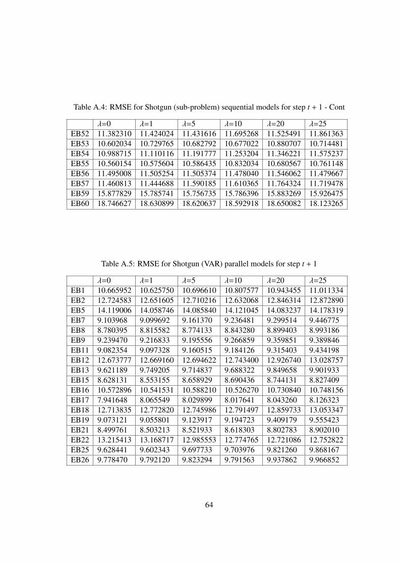
Table A.4: RMSE for Shotgun (sub-problem) sequential models for step t + 1 - Cont

λ=0 λ=1 λ=5 λ=10 λ=20 λ=25EB52 11.382310 11.424024 11.431616 11.695268 11.525491 11.861363EB53 10.602034 10.729765 10.682792 10.677022 10.880707 10.714481EB54 10.988715 11.110116 11.191777 11.253204 11.346221 11.575237EB55 10.560154 10.575604 10.586435 10.832034 10.680567 10.761148EB56 11.495008 11.505254 11.505374 11.478040 11.546062 11.479667EB57 11.460813 11.444688 11.590185 11.610365 11.764324 11.719478EB59 15.877829 15.785741 15.756735 15.786396 15.883269 15.926475EB60 18.746627 18.630899 18.620637 18.592918 18.650082 18.123265

Table A.5: RMSE for Shotgun (VAR) parallel models for step t + 1

λ=0 λ=1 λ=5 λ=10 λ=20 λ=25EB1 10.665952 10.625750 10.696610 10.807577 10.943455 11.011334EB2 12.724583 12.651605 12.710216 12.632068 12.846314 12.872890EB5 14.119006 14.058746 14.085840 14.121045 14.083237 14.178319EB7 9.103968 9.099692 9.161370 9.236481 9.299514 9.446775EB8 8.780395 8.815582 8.774133 8.843280 8.899403 8.993186EB9 9.239470 9.216833 9.195556 9.266859 9.359851 9.389846EB11 9.082354 9.097328 9.160515 9.184126 9.315403 9.434198EB12 12.673777 12.669160 12.694622 12.743400 12.926740 13.028757EB13 9.621189 9.749205 9.714837 9.688322 9.849658 9.901933EB15 8.628131 8.553155 8.658929 8.690436 8.744131 8.827409EB16 10.572896 10.541531 10.588210 10.526270 10.730840 10.748156EB17 7.941648 8.065549 8.029899 8.017641 8.043260 8.126323EB18 12.713835 12.772820 12.745986 12.791497 12.859733 13.053347EB19 9.073121 9.055801 9.123917 9.194723 9.409179 9.555423EB21 8.499761 8.503213 8.521933 8.618303 8.802783 8.902010EB22 13.215413 13.168717 12.985553 12.774765 12.721086 12.752822EB25 9.628441 9.602343 9.697733 9.703976 9.821260 9.868167EB26 9.778470 9.792120 9.823294 9.791563 9.937862 9.966852

64

Table A.6: RMSE for Shotgun (VAR) parallel models for step t + 1 - cont

λ=0 λ=1 λ=5 λ=10 λ=20 λ=25EB27 8.959297 8.923850 8.993795 8.984736 9.037680 9.083018EB29 10.100934 10.182273 10.129151 10.207267 10.245340 10.343201EB30 9.429308 9.465960 9.506073 9.582071 9.720019 9.698616EB31 8.991319 9.054918 8.987366 9.077259 9.104568 9.159902EB34 11.463263 11.524909 11.628098 11.597604 11.738466 11.847535EB35 9.509872 9.449744 9.542949 9.583424 9.723889 9.809498EB36 8.303484 8.327932 8.325977 8.340030 8.445074 8.488888EB37 8.932369 8.961635 8.996877 9.049976 9.160925 9.351486EB38 14.620485 14.633555 14.561646 14.648728 14.626025 14.662234EB41 10.472043 10.484694 10.452113 10.491764 10.533750 10.507888EB42 11.411532 11.496782 11.413600 11.540042 11.546437 11.661908EB43 9.113517 9.134220 9.124291 9.224713 9.318149 9.390601EB46 9.741903 9.791242 9.877178 9.854896 9.971411 9.972026EB47 11.626979 11.632774 11.662690 11.669133 11.777244 11.827230EB48 9.664486 9.698822 9.712971 9.741334 9.815352 9.870601EB49 8.391398 8.343886 8.389477 8.495626 8.563236 8.574860EB50 19.370856 19.510403 19.784692 19.590385 19.769616 19.791799EB51 9.812268 9.730085 9.721520 9.871570 9.940913 9.930556EB52 10.924502 10.868753 10.919280 11.043302 11.077608 11.126265EB53 10.163562 10.198336 10.190414 10.231500 10.289093 10.369056EB54 10.426904 10.354985 10.484538 10.535886 10.665387 10.802305EB55 9.696142 9.755260 9.821364 9.796089 9.969708 10.038167EB56 11.240105 11.243957 11.219188 11.244791 11.218100 11.248188EB57 10.672590 10.649964 10.635292 10.741745 10.802882 10.954785EB59 14.350273 14.337955 14.345249 14.312973 14.398551 14.415119EB60 18.468650 18.551048 18.226164 18.276358 18.138643 18.008690

Table A.7: RMSE for Shotgun (VAR) sequential models for step t + 1

λ=0 λ=1 λ=5 λ=10 λ=20 λ=25EB1 10.027665 10.041143 9.907361 9.801892 9.907258 9.951887EB2 12.384064 12.011183 11.655190 11.557796 11.542091 11.329968EB5 12.717599 12.764940 12.759193 12.917844 13.088269 13.034507EB7 8.413031 8.361496 8.297907 8.268324 8.311341 8.349406EB8 8.303415 8.227405 8.093144 7.916366 7.942831 7.914848EB9 8.234984 8.213827 8.258266 8.301793 8.376140 8.373069EB11 8.455508 8.486287 8.384233 8.110261 8.187524 8.198752EB12 11.454541 11.522492 11.602829 11.590692 11.917472 11.850973

65

Table A.8: RMSE for Shotgun (VAR) sequential models for step t + 1 - Cont

λ=0 λ=1 λ=5 λ=10 λ=20 λ=25EB13 9.262514 9.197713 8.878939 8.816613 8.814769 8.767165EB15 8.065865 8.114252 7.953734 7.836732 7.887419 7.862377EB16 9.704685 9.599857 9.427050 9.406739 9.505546 9.509283EB17 7.042478 7.034151 6.992339 6.955619 7.091199 6.964848EB18 11.800862 11.542340 11.314088 11.176373 11.379389 11.279215EB19 8.188251 8.202541 8.065439 8.057486 8.293380 8.335742EB21 7.816370 7.790034 7.825210 7.849603 7.950338 7.983583EB22 11.784932 11.670028 11.437068 11.239846 11.227034 11.163871EB25 9.051958 8.978185 8.841523 8.587392 8.634360 8.612475EB26 9.588619 9.593732 9.368735 9.181736 9.149234 9.112793EB27 8.482971 8.467663 8.458671 8.452309 8.499862 8.490150EB29 9.574105 9.497455 9.462161 9.243663 9.190317 9.157460EB30 8.633334 8.561307 8.511582 8.484008 8.670954 8.711327EB31 8.463992 8.587037 8.355974 8.297258 8.347291 8.382909EB34 10.804513 10.523001 10.305122 10.440943 10.684514 10.528163EB35 8.562945 8.493027 8.618893 8.601917 8.756966 8.751877EB36 7.785218 7.706048 7.660264 7.683854 7.776784 7.775625EB37 7.987037 8.026290 7.958808 7.922865 8.150582 8.127994EB38 15.548081 15.054927 14.676714 13.860060 13.756526 13.761961EB41 9.857355 9.817029 9.830477 9.747978 9.842589 9.833332EB42 10.550017 10.585495 10.247274 10.188395 10.359411 10.314479EB43 8.473145 8.470030 8.460279 8.229060 8.316450 8.344913EB46 8.832381 8.940285 8.874376 8.740800 8.892187 8.892916EB47 10.817422 10.838414 10.642048 10.653647 10.935768 10.893387EB48 9.092363 9.020881 8.899929 8.760768 8.769919 8.749062EB49 7.718090 7.701664 7.661776 7.565428 7.652677 7.671711EB50 17.861384 17.692084 17.638500 16.666856 16.739866 16.307117EB51 9.056430 8.986727 8.973245 8.864300 8.916608 8.895052EB52 9.730497 9.788165 9.824985 9.791974 10.002739 9.976032EB53 9.277028 9.379934 9.354667 9.216073 9.232325 9.255109EB54 9.563529 9.511069 9.331924 9.323041 9.430756 9.451937EB55 9.302087 9.176510 8.989231 8.907918 8.793240 8.757481EB56 9.541285 9.571548 9.744272 9.596240 10.167892 10.005188EB57 9.878972 9.720112 9.598006 9.546560 9.560144 9.557702EB59 13.875663 13.834108 13.445643 13.064717 13.133901 12.985007EB60 17.574259 17.248951 17.496836 17.329350 17.443331 17.585975

66

Appendix B

RMSE

This appendix intends to show the error plots of the models.

Figure B.1: Shotgun (sub-problem) sequential models RMSE for t + 1

67

Figure B.2: Shotgun (sub-problem) Sequential models RMSE for t + 6

68

Figure B.3: GRock (sub-problem) parallel models RMSE for t + 1

69

Figure B.4: GRock (sub-problem) parallel models RMSE for t + 6

70

Figure B.5: Shotgun (sub-problem) sequential RMSE for step t + 1. Models λ = 0, λ =

1 and λ = 5

71

Figure B.6: Shotgun (VAR) sequential RMSE for step t+1. Models λ = 0, λ = 10 and λ =

25

72

Figure B.7: Shotgun (Sub-problems) parallel RMSE for step t + 1. Models λ = 0, λ =

10 and λ = 5

73

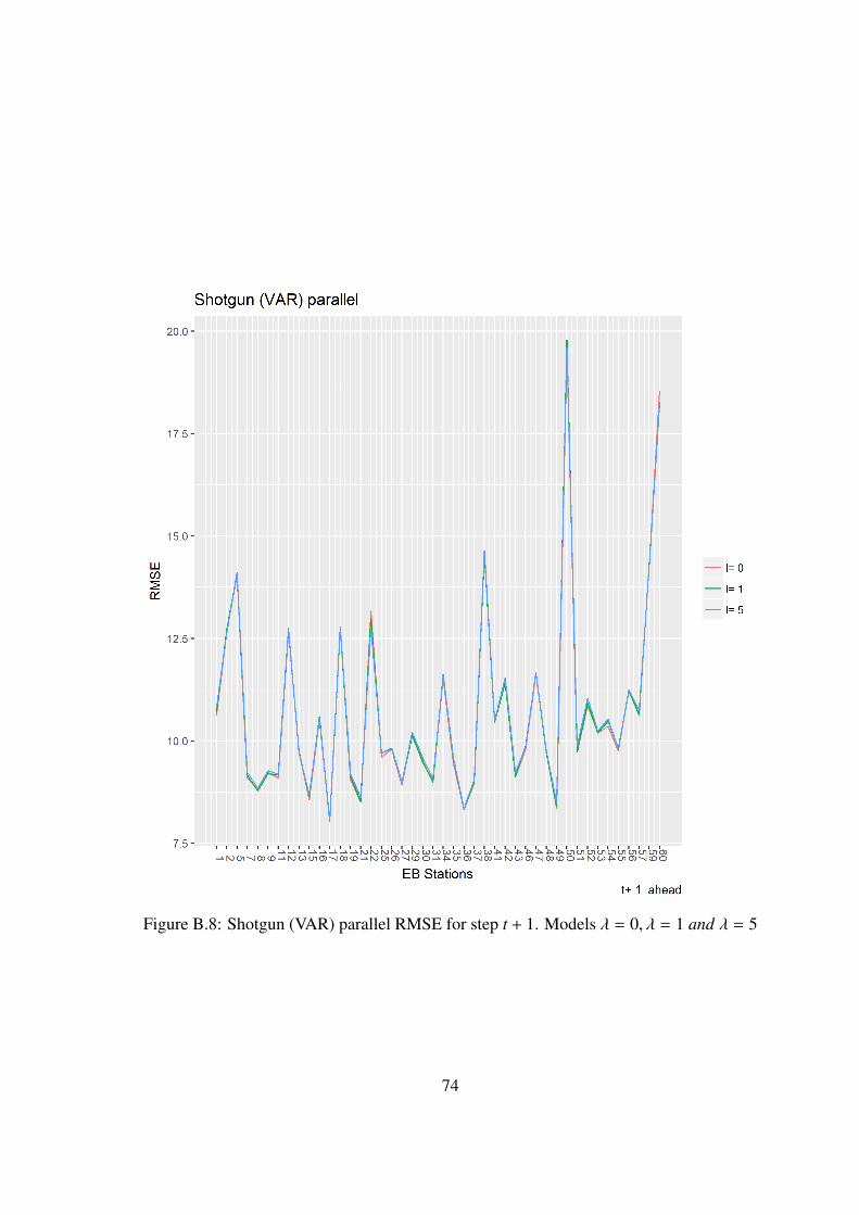
Figure B.8: Shotgun (VAR) parallel RMSE for step t + 1. Models λ = 0, λ = 1 and λ = 5

74

Appendix C

Forecast

In this appendix, we can see some extra examples of the forecast, for both approaches tothe problem as well as the programming techniques applied.

Figure C.1: EB17 Shotgun (sub-problem) parallel models’step t + 1 forecast for 2012-06

75

Figure C.2: EB18 GRock (sub-problem) Sequential models’step t + 1 forecast for period2012-02-02/2012-02-04

Figure C.3: EB18 GRock (sub-problem) Sequential models’step t + 6 forecast for period2012-02-02/2012-02-04

76

Figure C.4: EB18 GRock (VAR) Parallel models’step t + 1 forecast for 2012-09

Figure C.5: EB18 GRock (VAR) Parallel models’step t + 6 forecast for 2012-09

77

Figure C.6: EB18 GRock (VAR) Sequential models’step t + 1 forecast for 2012-09

Figure C.7: EB18 GRock (VAR) Sequential models’step t + 6 forecast for 2012-09

78

Figure C.8: EB1 Shotgun (VAR) Sequential models’step t + 1 forecast for 2013-01

Figure C.9: EB1 Shotgun (VAR) Sequential models’step t + 6 forecast for 2013-01

79

Figure C.10: EB1 Shotgun (VAR) Sequential models’step t + 1 forecast for 2013-01

Figure C.11: EB1 Shotgun (VAR) Sequential models’step t + 6 forecast for 2013-01

80

Bibliography

Peder Bacher, Henrik Madsen, and Henrik Aalborg Nielsen. Online short-term so-lar power forecasting. Solar Energy, 83(10):1772 – 1783, 2009. ISSN 0038-092X. doi: http://dx.doi.org/10.1016/j.solener.2009.05.016. URL http://www.sciencedirect.com/science/article/pii/S0038092X09001364.

R.J. Bessa, A. Trindade, and V. Miranda. Spatial-temporal solar power forecasting forsmart grids. Industrial Informatics, IEEE Transactions on, 11(1):232–241, Feb 2015.ISSN 1551-3203. doi: 10.1109/TII.2014.2365703.

Stephen Boyd and Lieven Vandenberghe. Convex Optimization. Cambridge UniversityPress, New York, NY, USA, 2004. ISBN 0521833787.

Joseph K. Bradley, Aapo Kyrola, Danny Bickson, and Carlos Guestrin. Parallel coordinatedescent for l1-regularized loss minimization. CoRR, abs/1105.5379, 2011. URL http://arxiv.org/abs/1105.5379.

J.C. Cao and S.H. Cao. Study of forecasting solar irradiance using neural net-works with preprocessing sample data by wavelet analysis. Energy, 31(15):3435 – 3445, 2006. ISSN 0360-5442. doi: http://dx.doi.org/10.1016/j.energy.2006.04.001. URL http://www.sciencedirect.com/science/article/pii/S0360544206001009. {ECOS} 2004 - 17th International Conference on Efficiency,Costs, Optimization, Simulation, and Environmental Impact of Energy on Process Sys-tems17th International Conference on Efficiency, Costs, Optimization, Simulation, andEnvironmental Impact of Energy on Process Systems.

Jiacong Cao and Xingchun Lin. Application of the diagonal recurrent wavelet neu-ral network to solar irradiation forecast assisted with fuzzy technique. Engineer-ing Applications of Artificial Intelligence, 21(8):1255 – 1263, 2008. ISSN 0952-1976. doi: http://dx.doi.org/10.1016/j.engappai.2008.02.003. URL http://www.sciencedirect.com/science/article/pii/S0952197608000092.

Shuanghua Cao and Jiacong Cao. Forecast of solar irradiance using recurrent neu-ral networks combined with wavelet analysis. Applied Thermal Engineering, 25:161 – 172, 2005. ISSN 1359-4311. doi: http://dx.doi.org/10.1016/j.applthermaleng.

81

2004.06.017. URL http://www.sciencedirect.com/science/article/pii/S1359431104001814.

Volkan Cevher, Stephen Becker, and Mark Schmidt. Convex optimization for big data.CoRR, abs/1411.0972, 2014. URL http://arxiv.org/abs/1411.0972.

Chi Wai Chow, Bryan Urquhart, Matthew Lave, Anthony Dominguez, Jan Kleissl, JanetShields, and Byron Washom. Intra-hour forecasting with a total sky imager at the{UC} san diego solar energy testbed. Solar Energy, 85(11):2881 – 2893, 2011. ISSN0038-092X. doi: http://dx.doi.org/10.1016/j.solener.2011.08.025. URL http://www.sciencedirect.com/science/article/pii/S0038092X11002982.

Hadja Maïmouna Diagne, Philippe Lauret, and Mathieu David. Solar irradi-ation forecasting: state-of-the-art and proposition for future developments forsmall-scale insular grids. In WREF 2012-World Renewable Energy Forum,2012. URL https://ases.conference-services.net/resources/252/2859/pdf/SOLAR2012_0617_full%20paper.pdf.

Maimouna Diagne, Mathieu David, Philippe Lauret, John Boland, and Nicolas Schmutz.Review of solar irradiance forecasting methods and a proposition for small-scale in-sular grids. Renewable and Sustainable Energy Reviews, 27:65 – 76, 2013. ISSN1364-0321. doi: http://dx.doi.org/10.1016/j.rser.2013.06.042. URL http://www.sciencedirect.com/science/article/pii/S1364032113004334.

Bihter Yerli Mustafa Kemal Kaymak Ahmet Duran Sahin Ercan Izgi, Ahmet Öztopal.Short?mid-term solar power prediction by using artificial neural networks. Solar En-ergy, 86(2):725 – 733, 2012. ISSN 0038-092X. doi: http://dx.doi.org/10.1016/j.solener.2011.11.013. URL http://www.sciencedirect.com/science/article/pii/S0038092X11004245.

Olivier Fercoq and Peter Richtárik. Accelerated, parallel and proximal coordinate descent.CoRR, abs/1312.5799, 2013. URL http://arxiv.org/abs/1312.5799.

Olivier Fercoq, Zheng Qu, Peter Richtárik, and Martin Takác. Fast distributed coordinatedescent for non-strongly convex losses. IEEE Workshop on Machine Learning forSignal Processing, 2014, 2014. URL http://arxiv.org/pdf/1405.5300v2.pdf.

Faranak Golestaneha, Pierre Pinson, and Hoay Beng Gooi. Generation and evaluation ofspace-time trajectories of photovoltaic power. October 2015.

Jing Huang and Matthew Perry. A semi-empirical approach using gradient boosting andk-nearest neighbors regression for gefcom2014 probabilistic solar power forecasting.International Journal of Forecasting, pages –, 2015. ISSN 0169-2070. doi: http://dx.doi.org/10.1016/j.ijforecast.2015.11.002. URL http://www.sciencedirect.com/science/article/pii/S0169207015001375.

82

Rich H. Inman, Hugo T.C. Pedro, and Carlos F.M. Coimbra. Solar forecasting meth-ods for renewable energy integration. Progress in Energy and Combustion Science,39(6):535 – 576, 2013. ISSN 0360-1285. doi: http://dx.doi.org/10.1016/j.pecs.2013.06.002. URL http://www.sciencedirect.com/science/article/pii/S0360128513000294.

Vijai Thottathil Jayadevan, Jeffrey J Rodriguez, Vincent PA Lonij, and Alexander DCronin. Forecasting solar power intermittency using ground-based cloud imaging.2012.

Wu Ji and Keong Chan Chee. Prediction of hourly solar radiation using a novel hy-brid model of {ARMA} and {TDNN}. Solar Energy, 85(5):808 – 817, 2011. ISSN0038-092X. doi: http://dx.doi.org/10.1016/j.solener.2011.01.013. URL http://www.sciencedirect.com/science/article/pii/S0038092X11000259.

Jakub Konecný, Zheng Qu, and Peter Richtárik. Semi-stochastic coordinate descent.CoRR, abs/1412.6293, 2014. URL http://arxiv.org/abs/1412.6293.

V.P.A. Lonij, V.T. Jayadevan, A.E. Brooks, J.J. Rodriguez, K. Koch, M. Leuthold, andA.D. Cronin. Forecasts of pv power output using power measurements of 80 residentialpv installs. In Photovoltaic Specialists Conference (PVSC), 2012 38th IEEE, pages003300–003305, June 2012. doi: 10.1109/PVSC.2012.6318280.

E. Lorenz and D. Heinemann. 1.13 - prediction of solar irradiance and photovoltaicpower. In Ali Sayigh, editor, Comprehensive Renewable Energy, pages 239 – 292.Elsevier, Oxford, 2012. ISBN 978-0-08-087873-7. doi: http://dx.doi.org/10.1016/

B978-0-08-087872-0.00114-1. URL http://www.sciencedirect.com/science/article/pii/B9780080878720001141.

E. Lorenz, J. Hurka, D. Heinemann, and H.G. Beyer. Irradiance forecasting for the powerprediction of grid-connected photovoltaic systems. Selected Topics in Applied EarthObservations and Remote Sensing, IEEE Journal of, 2(1):2–10, March 2009. ISSN1939-1404. doi: 10.1109/JSTARS.2009.2020300.

Ricardo Marquez, Hugo T.C. Pedro, and Carlos F.M. Coimbra. Hybrid solar forecast-ing method uses satellite imaging and ground telemetry as inputs to {ANNs}. So-lar Energy, 92:176 – 188, 2013. ISSN 0038-092X. doi: http://dx.doi.org/10.1016/j.solener.2013.02.023. URL http://www.sciencedirect.com/science/article/pii/S0038092X13000881.

Adel Mellit and Alessandro Massi Pavan. A 24-h forecast of solar irradiance using ar-tificial neural network: Application for performance prediction of a grid-connected{PV} plant at trieste, italy. Solar Energy, 84(5):807 – 821, 2010. ISSN 0038-092X. doi: http://dx.doi.org/10.1016/j.solener.2010.02.006. URL http://www.sciencedirect.com/science/article/pii/S0038092X10000782.

83

C Monteiro, R Bessa, V Miranda, A Botterud, J Wang, G Conzelmann, et al. Windpower forecasting: state-of-the-art 2009. Technical report, Argonne National Labora-tory (ANL), 2009.

Yurii Nesterov. Efficiency of coordinate descent methods on huge-scale optimiza-tion problems. CORE Discussion Papers 2010002, Université catholique de Lou-vain, Center for Operations Research and Econometrics (CORE), 2010. URL http://EconPapers.repec.org/RePEc:cor:louvco:2010002.

W Nicholson, D Matteson, and Jacob Bien. Structured regularization for large vectorautoregressions. 2014.

Zhimin Peng, Ming Yan, and Wotao Yin. Parallel and distributed sparse optimization. InSignals, Systems and Computers, 2013 Asilomar Conference on, pages 659–646. IEEE,2013.

Zhimin Peng, Yangyang Xu, Ming Yan, and Wotao Yin. Arock: an algorithmic frameworkfor async-parallel coordinate updates. 2015. URL http://arxiv.org/pdf/1506.02396.pdf.

Zheng Qu and Peter Richtárik. Coordinate descent with arbitrary sampling I: algorithmsand complexity. CoRR, abs/1412.8060, 2014a. URL http://arxiv.org/abs/1412.8060.

Zheng Qu and Peter Richtárik. Coordinate descent with arbitrary sampling II: expectedseparable overapproximation. CoRR, abs/1412.8063, 2014b. URL http://arxiv.org/abs/1412.8063.

P. Richtárik and M. Takác. Parallel coordinate descent methods for big data optimization.ArXiv e-prints, December 2012.

Peter Richtárik and Martin Takác. On optimal probabilities in stochastic coordinate de-scent methods. CoRR, abs/1310.3438, 2013. URL http://arxiv.org/abs/1310.3438.

Mark Schmidt, Nicolas L. Roux, and Francis R. Bach. Convergence rates ofinexact proximal-gradient methods for convex optimization. In J. Shawe-Taylor, R.S. Zemel, P.L. Bartlett, F. Pereira, and K.Q. Weinberger, editors,Advances in Neural Information Processing Systems 24, pages 1458–1466.Curran Associates, Inc., 2011. URL http://papers.nips.cc/paper/4452-convergence-rates-of-inexact-proximal-gradient-methods-for-convex-optimization.pdf.

Shai Shalev-Shwartz and Ambuj Tewari. Stochastic methods for l1 regularized loss min-imization. In Proceedings of the 26th Annual International Conference on Machine

84

Learning, ICML 2009, Montreal, Quebec, Canada, June 14-18, 2009, pages 929–936, 2009. doi: 10.1145/1553374.1553493. URL http://doi.acm.org/10.1145/1553374.1553493.

Christopher Sims. Macroeconomics and reality. Econometrica, 48(1):1–48, 1980.URL http://EconPapers.repec.org/RePEc:ecm:emetrp:v:48:y:1980:i:1:p:1-48.

G.K. Singh. Solar power generation by pv (photovoltaic) technology: A review. En-ergy, 53:1 – 13, 2013. ISSN 0360-5442. doi: http://dx.doi.org/10.1016/j.energy.2013.02.057. URL http://www.sciencedirect.com/science/article/pii/S0360544213001758.

M.D. Tabone and D.S. Callaway. Modeling variability and uncertainty of photovoltaicgeneration: A hidden state spatial statistical approach. Power Systems, IEEE Transac-tions on, 30(6):2965–2973, Nov 2015. ISSN 0885-8950. doi: 10.1109/TPWRS.2014.2372751.

Rachael Tappenden, Peter Richtárik, and Jacek Gondzio. Inexact coordinate descent:Complexity and preconditioning. CoRR, abs/1304.5530, 2013. URL http://arxiv.org/abs/1304.5530.

Robert Tibshirani. Regression shrinkage and selection via the lasso. Journal of the RoyalStatistical Society, Series B, 58:267–288, 1994.

Artur Jorge Teixeira Trindade. Very short-term solar power forecast for mv/lv distributiongrids. Master’s thesis, Faculdade de Engenharia da Universidade do Porto, March 2014.

A.G.R. Vaz, B. Elsinga, W.G.J.H.M. van Sark, and M.C. Brito. An artificial neural net-work to assess the impact of neighbouring photovoltaic systems in power forecasting inutrecht, the netherlands. Renewable Energy, 85:631 – 641, 2016. ISSN 0960-1481. doi:http://dx.doi.org/10.1016/j.renene.2015.06.061. URL http://www.sciencedirect.com/science/article/pii/S0960148115300847.

Jianwu Zeng and Wei Qiao. Short-term solar power prediction using a support vectormachine. Renewable Energy, 52:118 – 127, 2013. ISSN 0960-1481. doi: http://dx.doi.org/10.1016/j.renene.2012.10.009. URL http://www.sciencedirect.com/science/article/pii/S0960148112006465.

85