Vapnik-Chervonenkis Dimension

Definition and Lower boundAdapted from Yishai Mansour

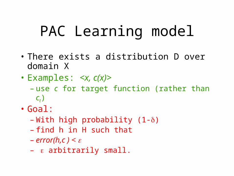
PAC Learning model

• There exists a distribution D over domain X

• Examples: <x, c(x)>– use c for target function (rather than ct)

• Goal: – With high probability (1-)– find h in H such that – error(h,c ) < – arbitrarily small.

VC: Motivation

• Handle infinite classes.• VC-dim “replaces” finite class size.• Previous lecture (on PAC):

– specific examples– rectangle.– interval.

• Goal: develop a general methodology.

The VC Dimension

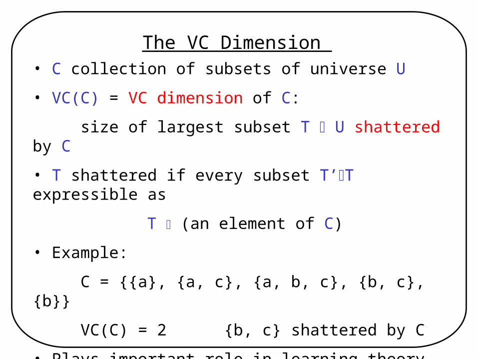
• C collection of subsets of universe U

• VC(C) = VC dimension of C:

size of largest subset T U shattered by C

• T shattered if every subset T’T expressible as

T (an element of C)

• Example:

C = {{a}, {a, c}, {a, b, c}, {b, c}, {b}}

VC(C) = 2 {b, c} shattered by C

• Plays important role in learning theory, finite automata, comparability theory, computational geometry

Definitions: Projection

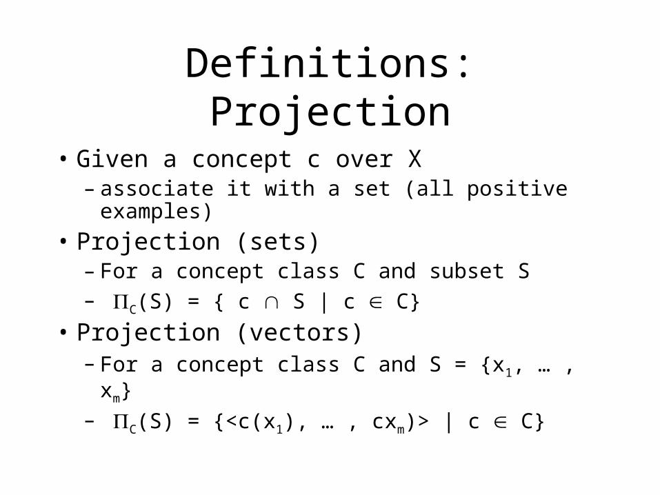
• Given a concept c over X– associate it with a set (all positive

examples)• Projection (sets)

– For a concept class C and subset S– C(S) = { c S | c C}

• Projection (vectors)– For a concept class C and S = {x1, … , xm}– C(S) = {<c(x1), … , cxm)> | c C}

Definition: VC-dim

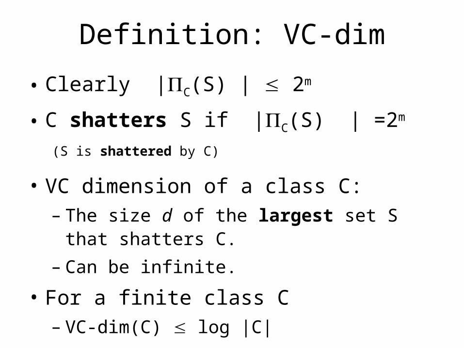
• Clearly |C(S) | 2m

• C shatters S if |C(S) | =2m

(S is shattered by C)

• VC dimension of a class C:– The size d of the largest set S that

shatters C.

– Can be infinite.

• For a finite class C– VC-dim(C) log |C|

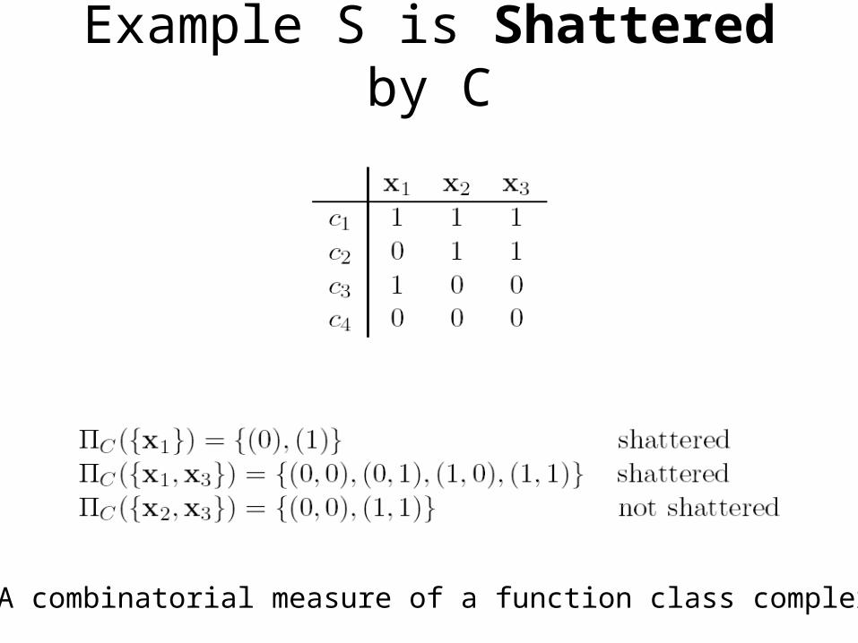
Example S is Shattered by C

VC: A combinatorial measure of a function class complexity

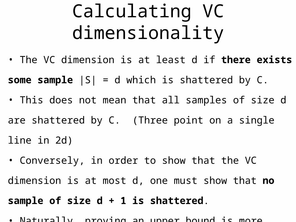
Calculating VC dimensionality

• The VC dimension is at least d if there exists some

sample |S| = d which is shattered by C.

• This does not mean that all samples of size d are

shattered by C. (Three point on a single line in 2d)

• Conversely, in order to show that the VC dimension is

at most d, one must show that no sample of size d + 1

is shattered.

• Naturally, proving an upper bound is more difficult than

proving the lower bound on the VC dimension.

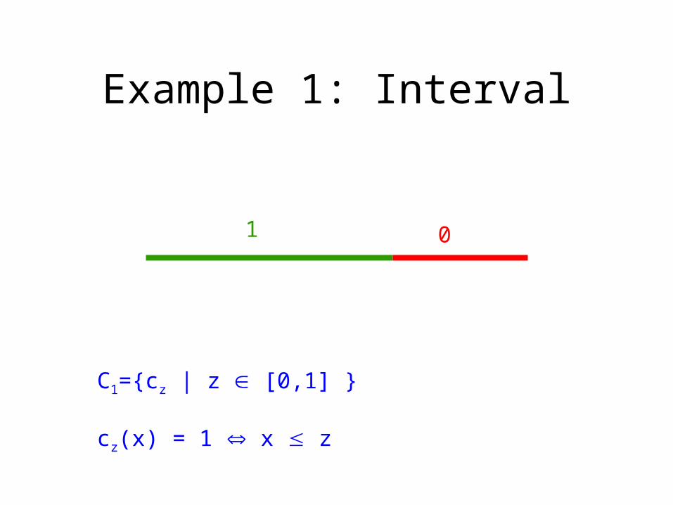
Example 1: Interval

1 0

C1={cz | z [0,1] }

cz(x) = 1 x z

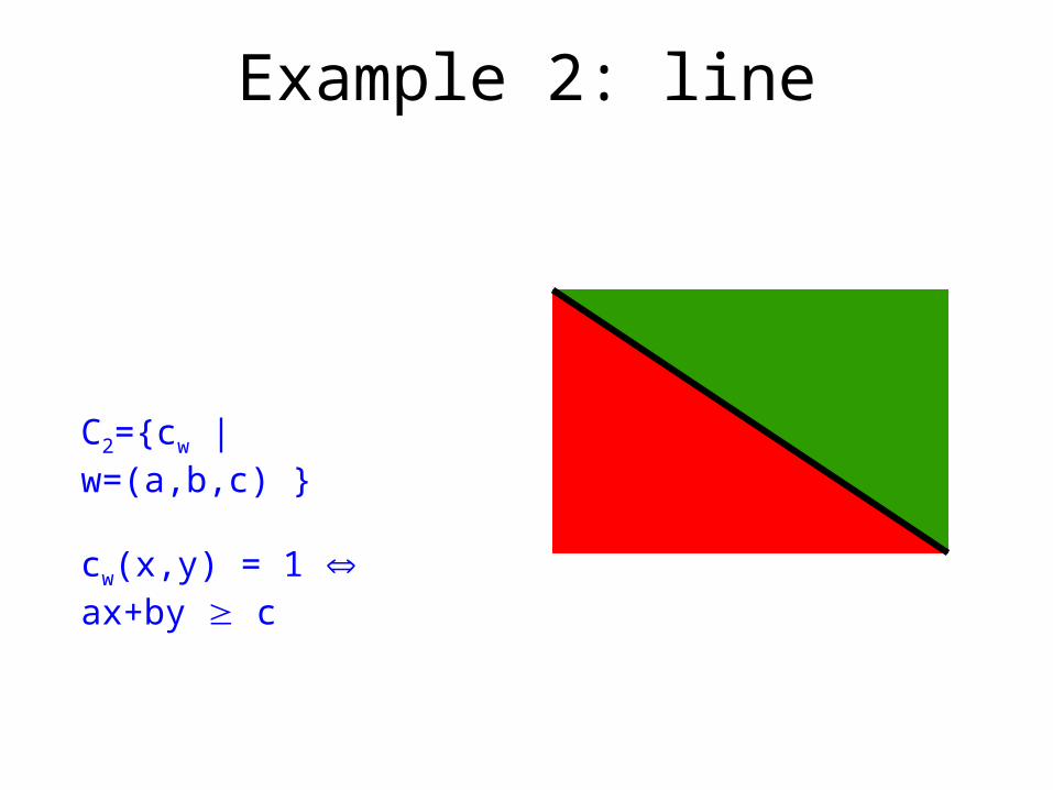
Example 2: line

C2={cw | w=(a,b,c) }

cw(x,y) = 1 ax+by c

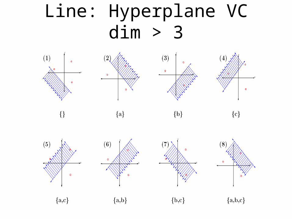
Line: Hyperplane VC dim > 3

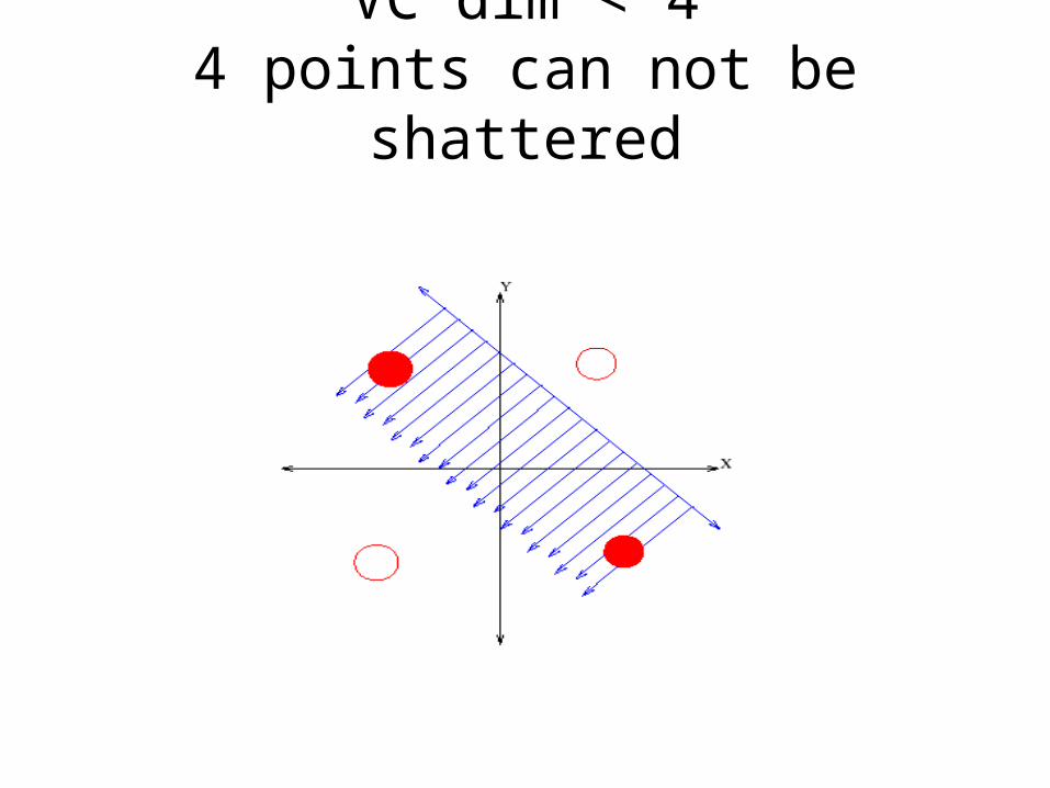
VC dim < 44 points can not be shattered

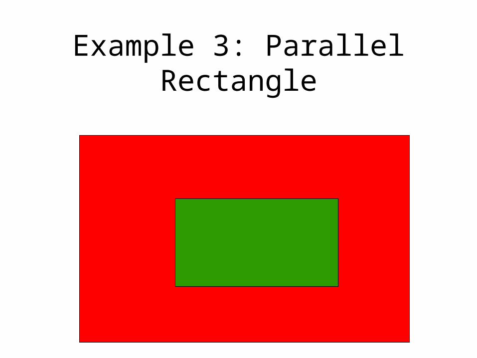
Example 3: Parallel Rectangle

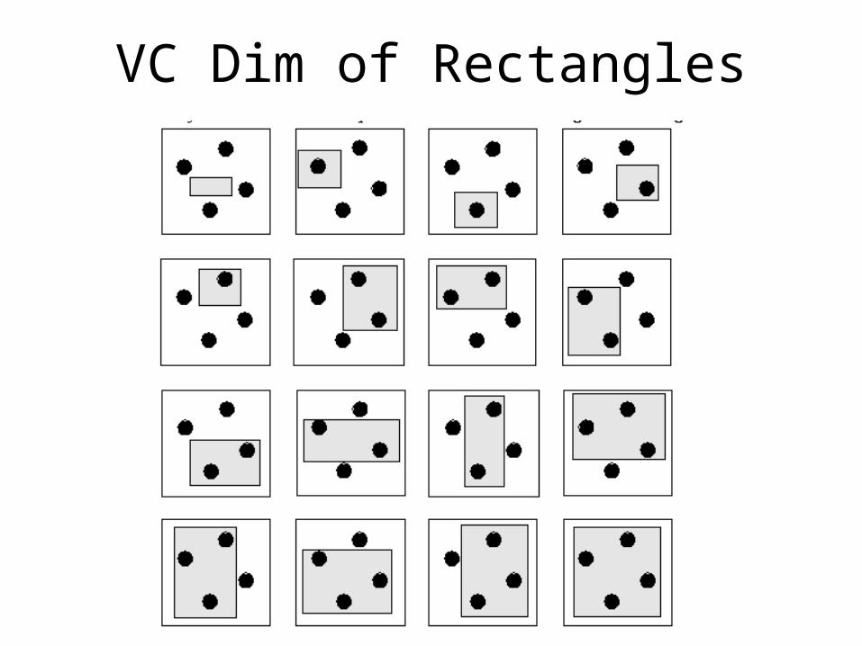
VC Dim of Rectangles

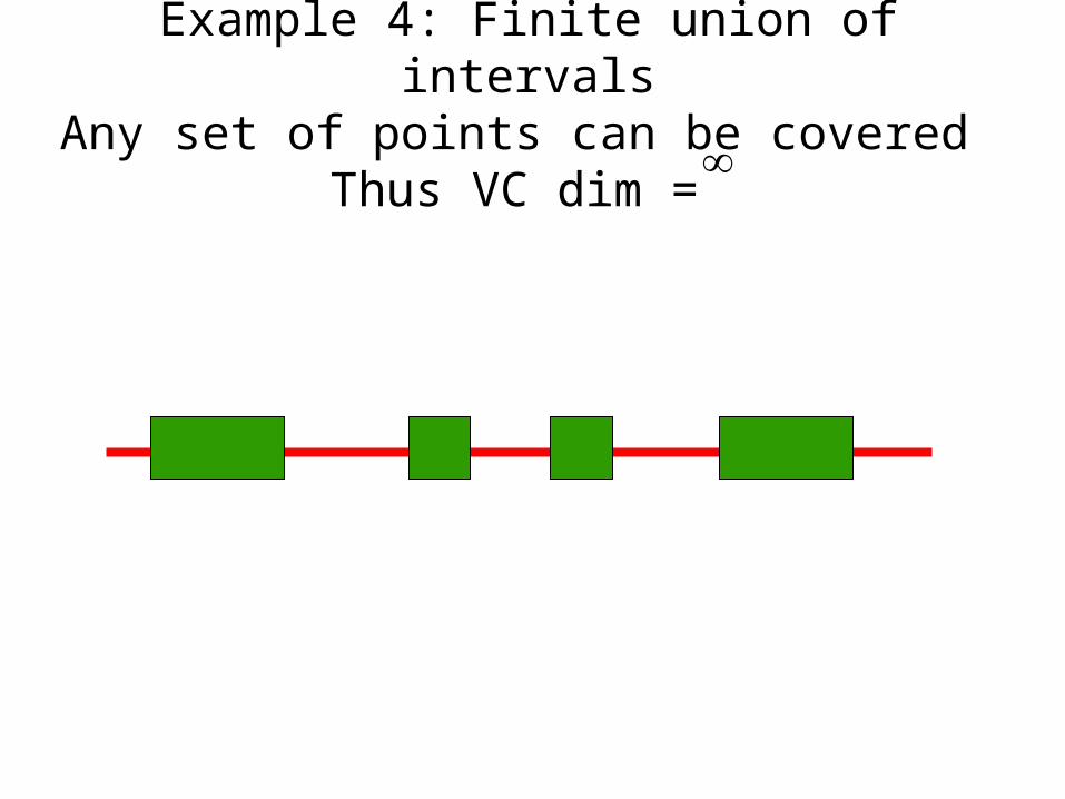
Example 4: Finite union of intervalsAny set of points can be covered

Thus VC dim =

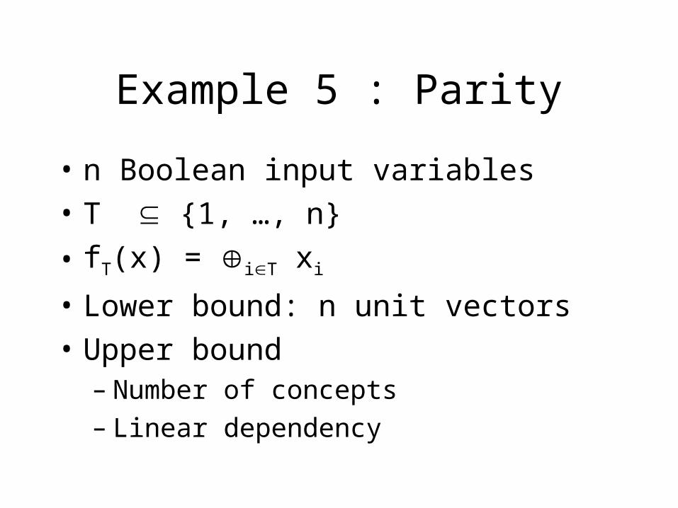
Example 5 : Parity

• n Boolean input variables• T {1, …, n}

• fT(x) = iT xi

• Lower bound: n unit vectors• Upper bound

– Number of concepts– Linear dependency

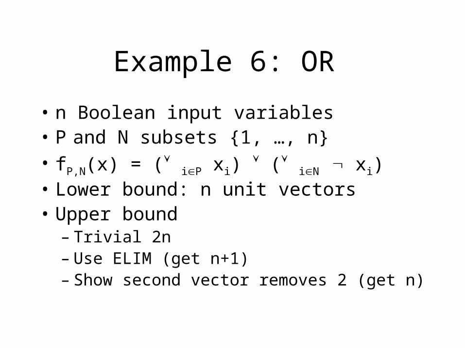
Example 6: OR

• n Boolean input variables• P and N subsets {1, …, n}• fP,N(x) = ( iP xi) ( iN xi)• Lower bound: n unit vectors• Upper bound

– Trivial 2n– Use ELIM (get n+1)– Show second vector removes 2 (get n)

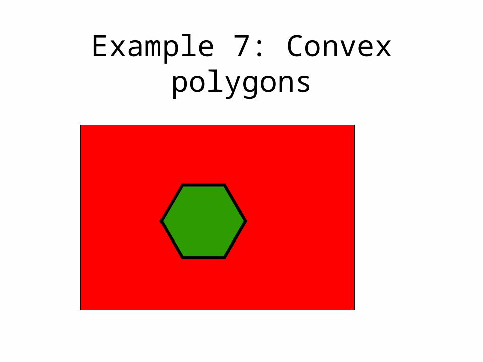
Example 7: Convex polygons

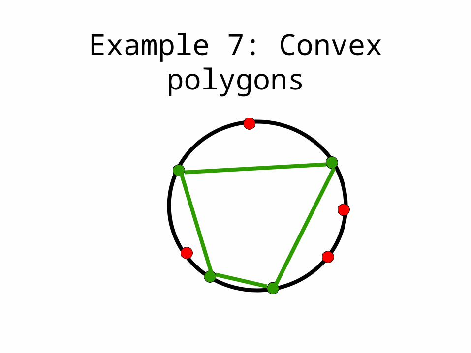
Example 7: Convex polygons

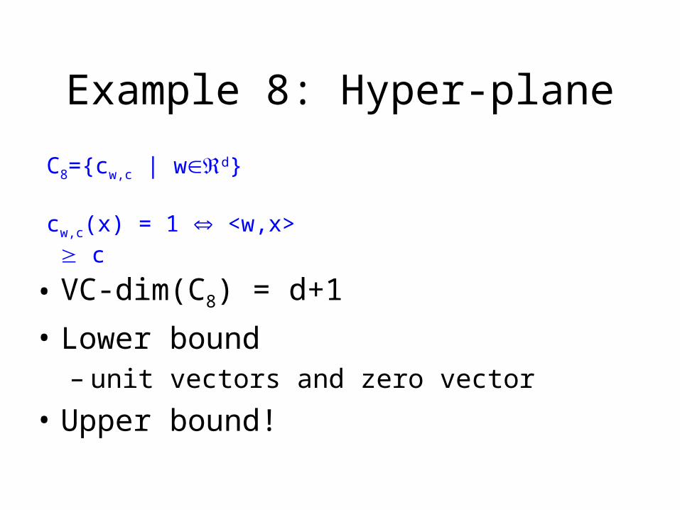
Example 8: Hyper-plane

• VC-dim(C8) = d+1

• Lower bound– unit vectors and zero vector

• Upper bound!

C8={cw,c | wd}

cw,c(x) = 1 <w,x> c

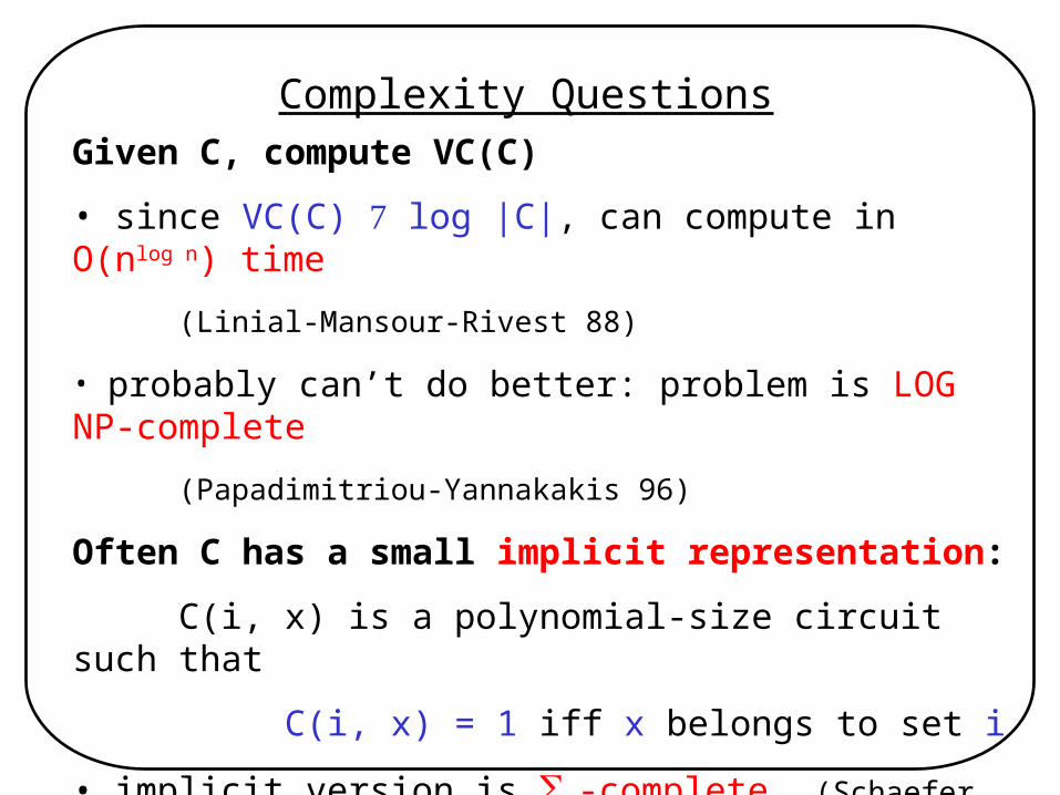
Complexity Questions

Given C, compute VC(C)

• since VC(C) log |C|, can compute in O(nlog n) time

(Linial-Mansour-Rivest 88)

• probably can’t do better: problem is LOG NP-complete

(Papadimitriou-Yannakakis 96)

Often C has a small implicit representation:

C(i, x) is a polynomial-size circuit such that

C(i, x) = 1 iff x belongs to set i

• implicit version is 3-complete (Schaefer 99)

(as hard as abc (a, b, c) for CNF formula )

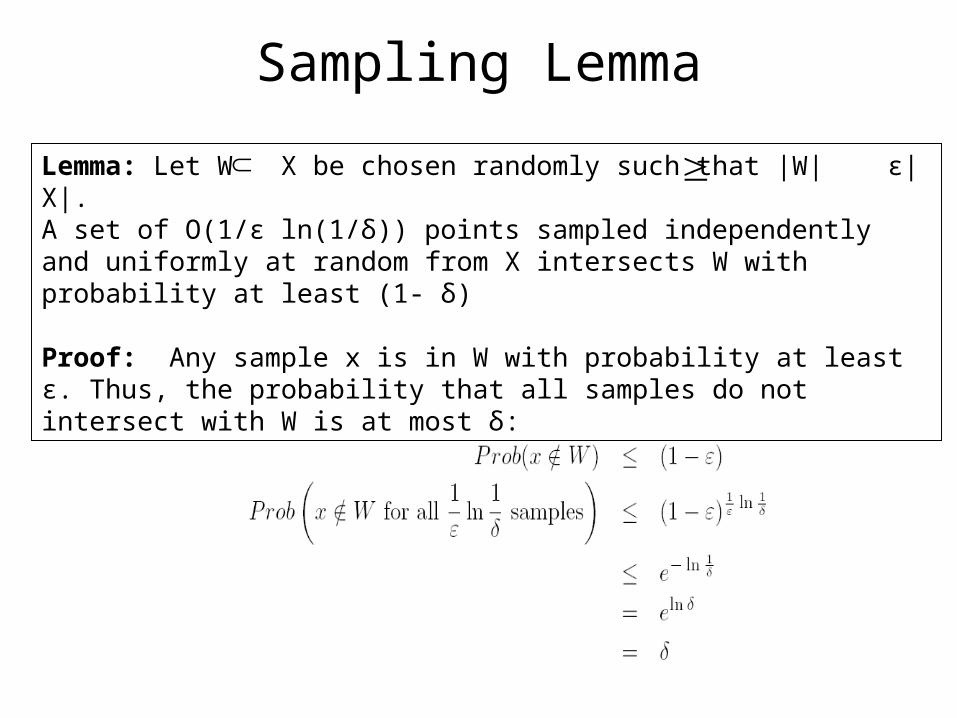
Sampling Lemma

Lemma: Let W X be chosen randomly such that |W| ε|X|. A set of O(1/ε ln(1/δ)) points sampled independently and uniformly at random from X intersects W with probability at least (1- δ)

Proof: Any sample x is in W with probability at least ε. Thus, the probability that all samples do not intersect with W is at most δ:

ε-Net Theorem

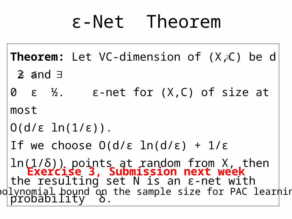
Theorem: Let VC-dimension of (X,C) be d 2

and

0 ε ½. ε-net for (X,C) of size at most

O(d/ε ln(1/ε)).

If we choose O(d/ε ln(d/ε) + 1/ε ln(1/δ)) points

at random from X, then the resulting set N is

an ε-net with probability δ. Exercise 3, Submission next week

A polynomial bound on the sample size for PAC learning

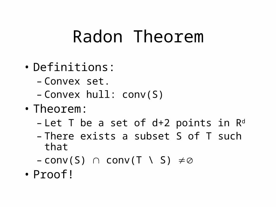
Radon Theorem

• Definitions:– Convex set.– Convex hull: conv(S)

• Theorem:– Let T be a set of d+2 points in Rd

– There exists a subset S of T such that– conv(S) conv(T \ S)

• Proof!

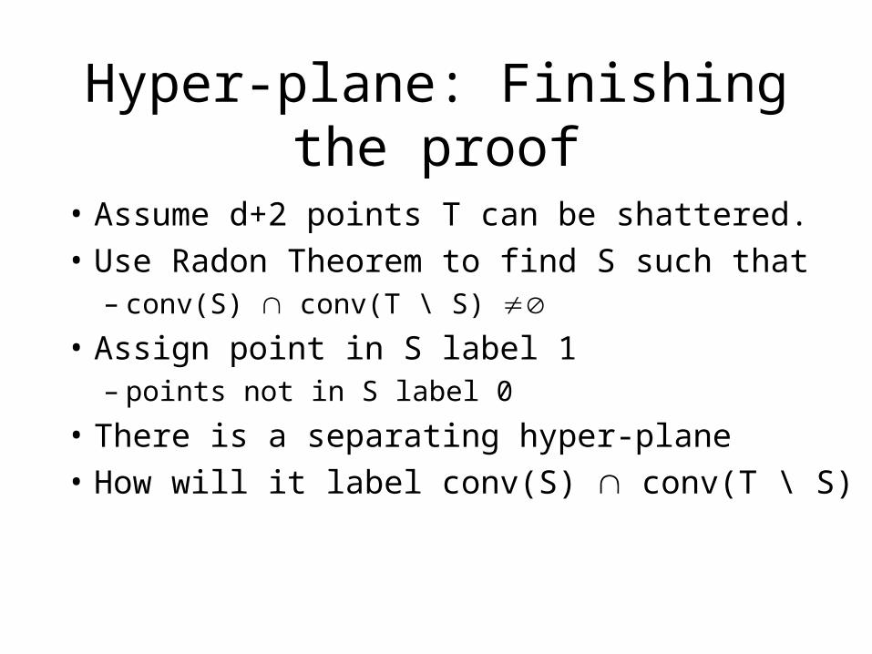
Hyper-plane: Finishing the proof

• Assume d+2 points T can be shattered.• Use Radon Theorem to find S such that

– conv(S) conv(T \ S)

• Assign point in S label 1– points not in S label 0

• There is a separating hyper-plane• How will it label conv(S) conv(T \ S)

Lower bounds: Setting

• Static learning algorithm:– asks for a sample S of size m()– Based on S selects a hypothesis

Lower bounds: Setting

• Theorem:– if VC-dim(C) = then C is not learnable.

• Proof:– Let m = m(0.1,0.1)– Find 2m points which are shattered (set T)– Let D be the uniform distribution on T– Set ct(xi)=1 with probability ½.

• Expected error ¼.• Finish proof!

Lower Bound: Feasible

• Theorem– VC-dim(C)=d+1, then m()=(d/)

• Proof:– Let T be a set of d+1 points which is

shattered.– D samples:

• z0 with prob. 1-8

• zi with prob. 8/d

Continue

– Set ct(z0)=1 and ct(zi)=1 with probability ½

• Expected error 2• Bound confidence

– for accuracy

Lower Bound: Non-Feasible

• Theorem– For two hypoth. m()=((log 1))

• Proof:– Let H={h0, h1}, where hb(x)=b

– Two distributions:

– D0: Prob. <x,1> is ½ - and <y,0> is ½ +

– D1: Prob. <x,1> is ½ + and <y,0> is ½ -