Eindhoven University of Technology Department of Biomedical Engineering Department of Electrical Engineering BIOMIM & Control Systems

Minimal Models for Glucose

and Insulin Kinetics

- A Matlab implementation -

NATAL VAN RIEL

version of February 5, 2004

1

Minimal Models for Glucose and Insulin Kinetics; a Matlab implementation by Natal van Riel, Eindhoven University of Technology 1 Introduction Minimal models of glucose and insulin plasma levels are commonly used to analyse the results of glucose tolerance tests in humans and laboratory animals (e.g. Dr. Richard N. Bergman and co-workers since the 1970's, see references [1]-[5]). In a typical frequently-sampled intravenous glucose tolerance test (FSIGTT), blood samples are taken from a fasting subject at regular intervals of time, following a single intravenous injection of glucose. The blood samples are then analyzed for glucose and insulin content. Fig. 1 shows a typical response from a normal subject.

Qualitatively, the glucose level in plasma starts at a peak due to the injection, drops to a minimum which is below the basal (pre-injection) glucose level, and then gradually returns to the basal level. The insulin level in plasma rapidly rises to a peak immediately after the injection, drops to a lower level which is still above the basal insulin level, rises again to a lesser peak, and then gradually drops to the basal level. Depending on the state of the subject, there can be wide variations from this response; for example, the glucose level may not drop below basal level, the first peak in insulin level may have different amplitude, there may be no secondary peak in insulin level, or there may be more than two peaks in insulin level. The glucose and insulin minimal models provide a quantitative and parsimonious description of glucose and insulin concentrations in the blood samples following the glucose injection. The glucose minimal model involves two physiologic compartments: a plasma compartment and an interstitial tissue compartment; the insulin minimal model involves only a single plasma compartment. The glucose and insulin minimal models allow us to characterize the FSIGT test data in terms of four metabolic indices: SI = insulin sensitivity: a measure of the dependence of fractional glucose disappearance on plasma insulin,

0 50 100 150 2000

50

100

150

insu

lin le

vel [ µ

U/m

L]

time [min]0 50 100 150 200

0

100

200

300

400

gluc

ose

leve

l [m

g/dL

]

time [min] Fig. 1 FSIGT test data from a normal subject ([3]). (See Appendix A for data table.)

2

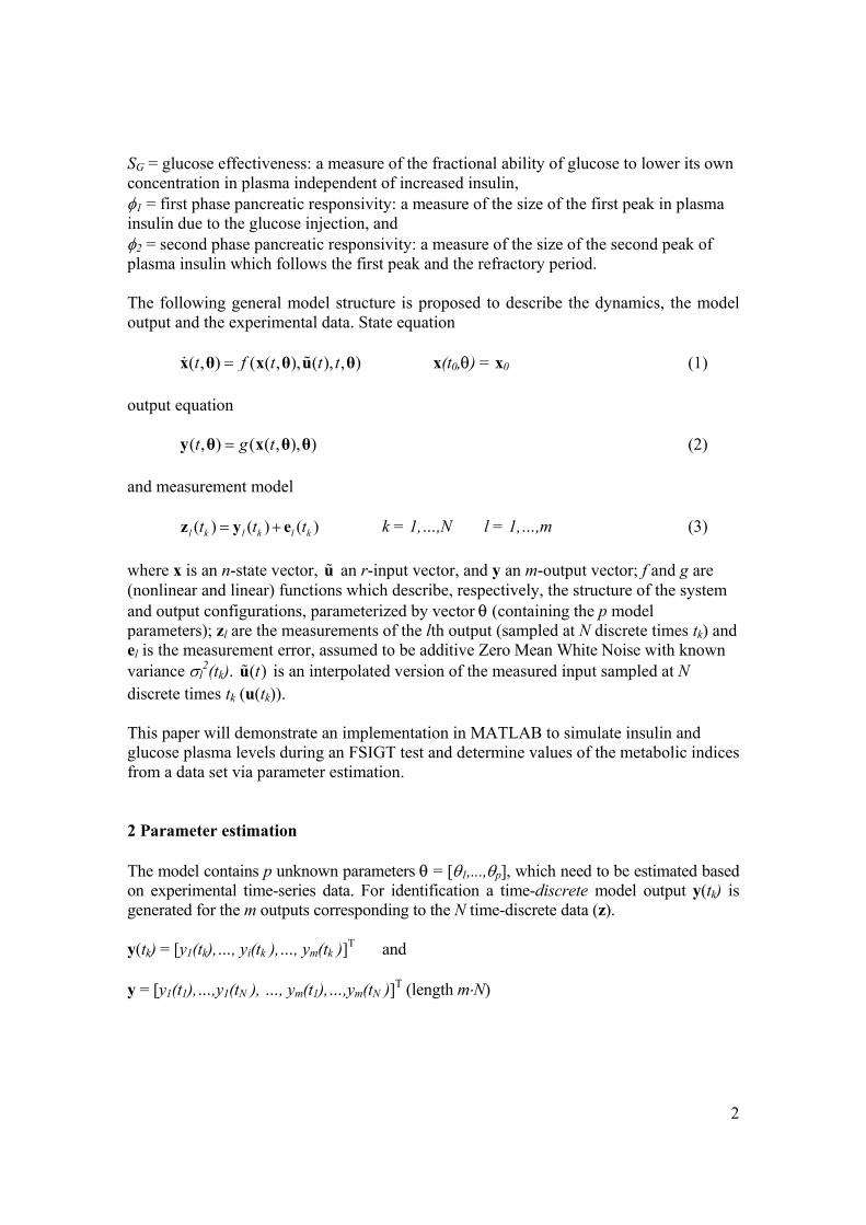
SG = glucose effectiveness: a measure of the fractional ability of glucose to lower its own concentration in plasma independent of increased insulin, φ1 = first phase pancreatic responsivity: a measure of the size of the first peak in plasma insulin due to the glucose injection, and φ2 = second phase pancreatic responsivity: a measure of the size of the second peak of plasma insulin which follows the first peak and the refractory period. The following general model structure is proposed to describe the dynamics, the model output and the experimental data. State equation

( , ) ( ( , ), ( ), , )t f t t t=x θ x θ u θ x(t0,θ) = x0 (1) output equation

( , ) ( ( , ), )t g t=y θ x θ θ (2) and measurement model

( ) ( ) ( )l k l k l kt t t= +z y e k = 1,…,N l = 1,…,m (3) where x is an n-state vector, u an r-input vector, and y an m-output vector; f and g are (nonlinear and linear) functions which describe, respectively, the structure of the system and output configurations, parameterized by vector θ (containing the p model parameters); zl are the measurements of the lth output (sampled at N discrete times tk) and el is the measurement error, assumed to be additive Zero Mean White Noise with known variance σl

2(tk). ( )tu is an interpolated version of the measured input sampled at N discrete times tk (u(tk)). This paper will demonstrate an implementation in MATLAB to simulate insulin and glucose plasma levels during an FSIGT test and determine values of the metabolic indices from a data set via parameter estimation. 2 Parameter estimation The model contains p unknown parameters θ = [θ1,...,θp], which need to be estimated based on experimental time-series data. For identification a time-discrete model output y(tk) is generated for the m outputs corresponding to the N time-discrete data (z). y(tk) = [y1(tk),…, yi(tk ),…, ym(tk )]T and y = [y1(t1),…,y1(tN ), …, ym(t1),…,ym(tN )]T (length m⋅N)

3

A commonly used estimation method is the Least Squares method. The difference between the measurements in column vector z and the time-discrete model output y (column vector), i.e. the model error (also referred to as the residuals), is weighted in a quadratic criterion:

( ) ( , , )k k kt t= −ε z y u θ (4)

1

ˆ( , )N

TN k k

kJ

=

= ∑u θ ε Wε (5)

where θ̂ is the vector of estimated parameters and W is a [m⋅N× m⋅N] positive definite symmetric* weighting matrix (the weighted Least Squares algorithm). The parameter estimate with N data samples is denoted by the hat ^ and the subscript N.

ˆ

ˆ ˆarg min ( , )N NJ≥

=θ 0

θ u θ (6)

Since the parameters have a physiological interpretation, they are bounded to ≥ 0. For the optimal estimates the functional J reaches a minimum. Due to the inherent model errors (model bias, variance error) a zero value of the identification function cannot be expected. If the weighting matrix W used in the least-squares fit is selected as the inverse of the data covariance matrix cov(z), according to the Gauss-Markov theorem, ˆ

Nθ is the minimum variance, unbiased estimate (Maximum Likelihood Estimate) and an estimate of the parameter accuracy can be obtained:

1ˆcov( )N−=θ F (7)

where F is the Fisher information matrix given by:

T

= ∂ ∂∂ ∂y yF Wθ θ

(8)

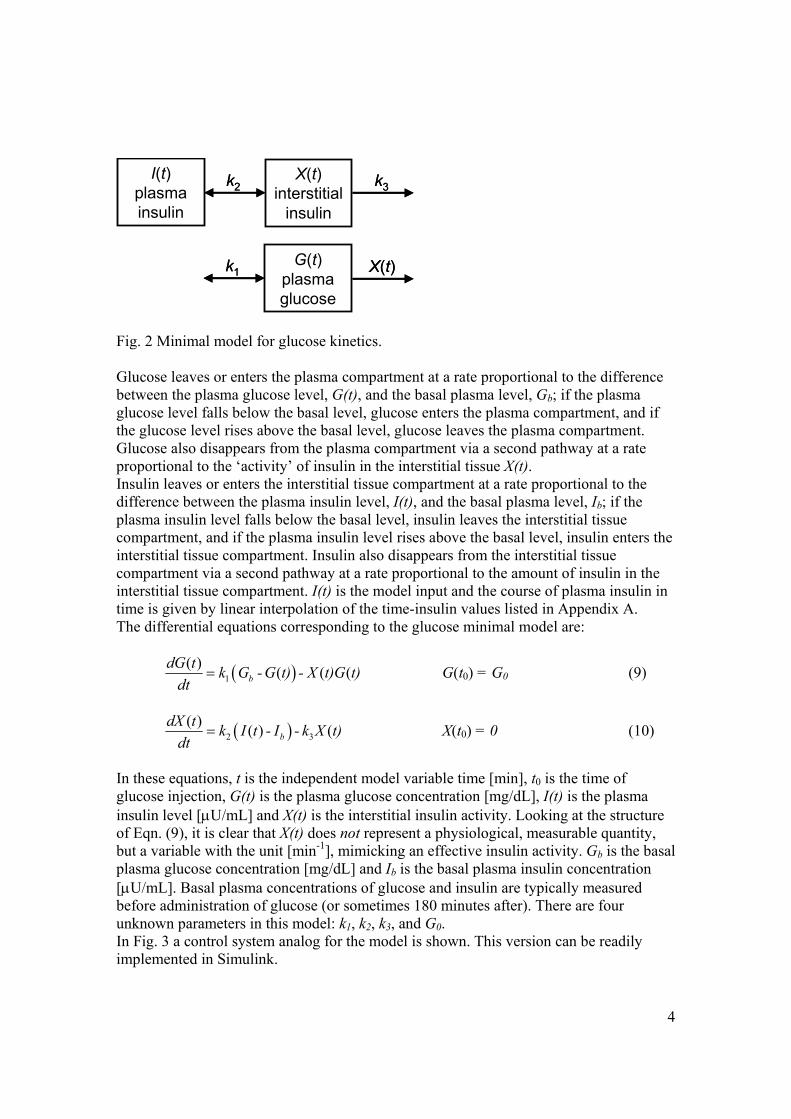
and ∂y/∂θ is the model output sensitivity (i.e. [6]). 3 Minimal model for glucose kinetics The diagram in Fig. 2 summarizes the minimal model for glucose kinetics.

* Thus W = WT (all eigenvalues real), xT W x > 0 (nonnegative eigenvalues).

4

Glucose leaves or enters the plasma compartment at a rate proportional to the difference between the plasma glucose level, G(t), and the basal plasma level, Gb; if the plasma glucose level falls below the basal level, glucose enters the plasma compartment, and if the glucose level rises above the basal level, glucose leaves the plasma compartment. Glucose also disappears from the plasma compartment via a second pathway at a rate proportional to the ‘activity’ of insulin in the interstitial tissue X(t). Insulin leaves or enters the interstitial tissue compartment at a rate proportional to the difference between the plasma insulin level, I(t), and the basal plasma level, Ib; if the plasma insulin level falls below the basal level, insulin leaves the interstitial tissue compartment, and if the plasma insulin level rises above the basal level, insulin enters the interstitial tissue compartment. Insulin also disappears from the interstitial tissue compartment via a second pathway at a rate proportional to the amount of insulin in the interstitial tissue compartment. I(t) is the model input and the course of plasma insulin in time is given by linear interpolation of the time-insulin values listed in Appendix A. The differential equations corresponding to the glucose minimal model are:

( )1( ) ( ( (b

dG t k G - G t) - X t)G t)dt

= G(t0) = G0 (9)

( )2 3( ) ( ) (b

dX t k I t - I - k X t)dt

= X(t0) = 0 (10)

In these equations, t is the independent model variable time [min], t0 is the time of glucose injection, G(t) is the plasma glucose concentration [mg/dL], I(t) is the plasma insulin level [µU/mL] and X(t) is the interstitial insulin activity. Looking at the structure of Eqn. (9), it is clear that X(t) does not represent a physiological, measurable quantity, but a variable with the unit [min-1], mimicking an effective insulin activity. Gb is the basal plasma glucose concentration [mg/dL] and Ib is the basal plasma insulin concentration [µU/mL]. Basal plasma concentrations of glucose and insulin are typically measured before administration of glucose (or sometimes 180 minutes after). There are four unknown parameters in this model: k1, k2, k3, and G0. In Fig. 3 a control system analog for the model is shown. This version can be readily implemented in Simulink.

I(t)

plasma insulin

X(t)interstitial

insulin

G(t)plasma glucose

k3k3

X(t)X(t)k1k1

k2k2

Fig. 2 Minimal model for glucose kinetics.

5

Note that in this model, glucose is utilized at the constant rate k1, when we neglect feedback effects due to interstitial insulin as represented by the term −X(t)G(t). An additional amount of plasma insulin will cause the amount of interstitial insulin to change, which in turn, will cause the rate of glucose utilization to change. The insulin sensitivity is defined as SI = k2/k3 and the glucose effectiveness is defined as SG = k1. Equation 10 can be reformulated as:

( )( )3( ) ( ) (I b

dX t k S I t - I - X t)dt

= (11)

The MATLAB commands in the function-file "gluc_min_mod.m" (Appendix B) simulate the glucose profile given the time course of plasma insulin as model input signal. Both the built-in MATLAB ode-solvers (ode45) as well as forward Euler method can be used for integration. For the fixed time-step Euler method an integration step of

15 min( ( ))expt diffδ = t is used (i.e. one-fifth of the smallest experimental sample interval).

The plasma insulin concentration input signal is obtained by linear interpolation of the time-insulin values listed in Appendix A (MATLAB function interp1). If fixed step integration is used, the simulation time vector tsim is known beforehand and an interpolated input signal (vector) can be pre-calculated before the simulation starts. When a variable step solver is used, the interpolated input value has to be calculated in each simulation step, given the new time sample selected by the solver. The MATLAB commands in Appendix C ("gluc_mm_mle.m") estimate values for the parameters given the time course of plasma glucose. The values of the parameters found minimize (in the weighted least squares sense) the difference between the measured time course of plasma glucose and the parameter-dependent solution to the glucose minimal

1sk1k1

-

+

-

+

+

-

+

-

Gb

G(t)

1sk2k2

k3k3

-

+

-

+

-

+

-

+I(t)

Ib

X(t)

x

Fig. 3 Control system analog model for glucose kinetics.

6

model differential equations. The routine ‘lsqnonlin’ from the Optimization Toolbox is used. This function also returns the residuals ε at the solution ˆ

Nθ and the Jacobian which can be used to calculate the Fisher information matrix to obtain estimates of the parameter accuracy. 4 Results of glucose model The simulation results of the identified glucose minimal model are shown in Fig. 4.

The insulin sensitivity, SI, for this data set is estimated as 5.039 ×10−4 min−1⋅(µU/ml)−1 which is within the normal range reported in reference 2: 2.1 to 18.2 ×10−4 min−1⋅(µU/ml)−1. The glucose utilization, SG, for this data set is estimated as 0.0265 min−1, which is also within the normal range reported in reference 2: 0.0026 to 0.039 min−1. 5 Minimal model for insulin kinetics Instead of taking plasma glucose G(t) as output also plasma insulin I(t) can be considered as key variable to develop a model that interprets the FSIGT data. Next we examine the minimal model for insulin kinetics, which includes other metabolic indices than the

0 50 100 150 2000

100

200

300

400

gluc

ose

leve

l [m

g/dL

] model simulationexperimental test data

0 50 100 150 2000

50

100

150

insu

lin le

vel [ µ

U/m

L]

time [min]

interpolated measured test data

0 50 100 150 200-5

0

5

10x 10

-3

time [min]

inte

rstit

ial i

nsul

in [1

/min

]

Fig. 4 Simulation results of the glucose minimal model for a normal subject. Solid lines:

simulation results, circles: data. G0 = 279 [mg⋅dL-1], SG = 2.6e-2 [min-1], k3 = 0.025 [min-1] and SI = 5.0e-4 [mL⋅µU-1⋅min-1].

7

glucose minimal model. Now the course of plasma glucose in time, G(t), is the input and is given by linear interpolation of the time-glucose values listed in Appendix A. The diagram in Fig. 5 summarizes the minimal model for insulin kinetics.

Insulin enters the plasma insulin compartment at a rate proportional to the product of time and the concentration of glucose above a threshold amount GT. Here, time is the interval t-t0, in minutes, from the glucose injection. If the plasma glucose level drops below the threshold amount, the rate of insulin entering the plasma compartment is zero. Insulin is cleared from the plasma compartment at a rate proportional to the amount of insulin in the plasma compartment. The minimal model for insulin kinetics is given by the equation:

( ) 0( ( ) ( ) if ( )( )( )

T TG t) G t t kI t G t GdI tdt kI t

γ − − − >=

− I(t0) = I0 (12)

k is the insulin clearance fraction, GT is roughly the basal glucose plasma level, and γ is a measure of the secondary pancreatic response to glucose. The first phase pancreatic responsivity is defined as φ1 = (Imax−Ib)/[k·(G0−Gb)] where Imax is the maximum insulin response. The second phase pancreatic responsivity is defined as φ2 = γ×104. The model involves an input event switch and the combination of discrete and continuous characteristics (a hybrid control system). The simulation model has been implemented in MATLAB similar to the glucose minimal model and the parameters estimation routine has been modified to estimate k, γ, GT and I0. Results are shown in Fig. 6.

γ(t-t0)γ(t-t0) kkI(t)plasma insulin

Fig. 5 Minimal model for insulin kinetics.

8

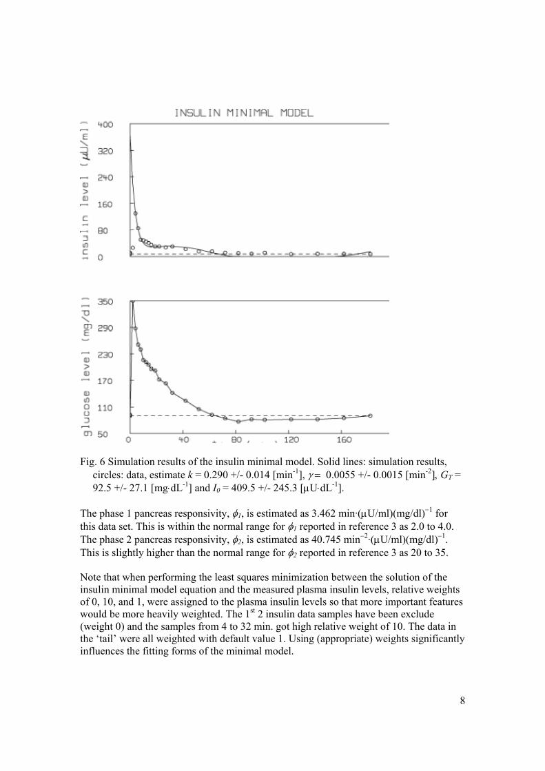
The phase 1 pancreas responsivity, φ1, is estimated as 3.462 min·(µU/ml)(mg/dl)−1 for this data set. This is within the normal range for φ1 reported in reference 3 as 2.0 to 4.0. The phase 2 pancreas responsivity, φ2, is estimated as 40.745 min−2·(µU/ml)(mg/dl)−1. This is slightly higher than the normal range for φ2 reported in reference 3 as 20 to 35. Note that when performing the least squares minimization between the solution of the insulin minimal model equation and the measured plasma insulin levels, relative weights of 0, 10, and 1, were assigned to the plasma insulin levels so that more important features would be more heavily weighted. The 1st 2 insulin data samples have been exclude (weight 0) and the samples from 4 to 32 min. got high relative weight of 10. The data in the ‘tail’ were all weighted with default value 1. Using (appropriate) weights significantly influences the fitting forms of the minimal model.

Fig. 6 Simulation results of the insulin minimal model. Solid lines: simulation results,

circles: data, estimate k = 0.290 +/- 0.014 [min-1], γ = 0.0055 +/- 0.0015 [min-2], GT = 92.5 +/- 27.1 [mg⋅dL-1] and I0 = 409.5 +/- 245.3 [µU⋅dL-1].

9

6 Combined minimal model The glucose minimal model provides differential equations for the plasma glucose and interstitial insulin levels. The insulin minimal model provides a differential equation for the plasma insulin level. It is possible to combine all three differential equations into one model. This is demonstrated in the following do-file, GGI.DO.

7 Discussion

Fig. 7 Simulation results of the combined minimal model. Solid lines: simulation results,

circles: data. G0 = 279 [mg⋅dL-1], SG = 2.6e-2 [min-1], k3 = 0.025 [min-1], SI = 5.0e-4 [mL⋅µU-1⋅min-1], k = 0.27 [min-1], γ = 0.0041 [min-2], GT = 83.7 [mg⋅dL-1] and I0 = 363.7 [µU⋅dL-1].

10

These results show that there is not a unique set of parameters that characterize a FSIGT test data set. This appears to be common in the literature. The combined minimal model is seen to generate slightly lower values for glucose effectiveness and insulin sensitivity than the glucose minimal model, and slightly higher values for phase 1 and 2 pancreas responsivity than the insulin minimal model. Several authors have augmented the insulin minimum model to account for plasma levels of C-peptide (see references [7]-[9]). It is a straightforward exercise to implement the C-Peptide minimal model using MATLAB. This paper has shown how MATLAB can be used to calculate diagnostically important metabolic indices which arise in the glucose and insulin minimal models from frequently-sampled intravenous glucose tolerance test data. Comparison of the results of different models revealed a fundamental issue. Analysis of model structure and information content of the data can be used to further address this issue and analyze the bottlenecks. The results of such analysis can be used to design experiments (or modifications of the models) that will provide less ambiguous results. References [1] Saad, M.F., Anderson, R.L., Laws, A., Watanabe, R.M., Kades, W.W., Chen, Y.-D.I.,

Sands, R.E., Pei, D., Savage, P.J. and Bergman, R.N. (1994) A comparison between the minimal model and the glucose clamp in the assessment of insulin sensitivity across the spectrum of glucose tolerance. Diabetes 43: 1114-21.

[2] Steil, G.M., Volund, A., Kahn, S.E. and Bergman, R.N. (1993) Reduced sample number for calculation of insulin sensitivity and glucose effectiveness from the minimal model. Diabetes 42: 250-256.

[3] Pacini, G. and Bergman, R.N. (1986) MINMOD: a computer program to calculate insulin sensitivity and pancreatic responsivity from the frequently sampled intravenous glucose tolerance test. Computer Methods and Programs in Biomedicine 23: 113-122.

[4] Toffolo, G., Bergman, R.N., Finegood, D.T., Bowden, C.R. and Cobelli, C. (1980) Quantitative estimation of beta cell sensitivity to glucose in the intact organism - a minimal model of insulin kinetics in the dog. Diabetes 29: 979-990.

[5] Bergman, R.N., Ider, Y.Z., Bowden, C.R. and Cobelli, C. (1979) Quantitative estimation of insulin sensitivity. Am. J. Physiol. Endocrinol. Metab. 236: E667-677.

[6] Damen, A.A.H. lecture notes, Eindhoven University of Technology, The Netherlands, 2003.

[7] Watanabe, R.M., Volund, A., Roy, S. and Bergman, R.N. (1988) Prehepatic B-cell secretion during the intravenous glucose tolerance test in humans: application of a combined model of insulin and C-peptide kinetics, J. Clin. Endocrinology Metab. 69: 790-797.

[8] Cobelli, C. and Pacini, G. (1988) Insulin secretion and hepatic extraction in humans by minimal modeling of C-peptide and insulin kinetics. Diabetes 37: 223-231.

[9] Volund, A., Polonsky, K.S. and Bergman, R.N. (1987) Calculated pattern of intraportal insulin appearance without independent assessment of C-peptide kinetics. Diabetes 36: 1195-1202.

11

12

Appendix A: Experimental data Reference [3] provides the FSIGT test data (also shown in Fig. 1) from a normal individual:

time (minutes) glucose level (mg/dl) insulin level (µU/ml) 0 92 11 2 350 26 4 287 130 6 251 85 8 240 51 10 216 49 12 211 45 14 205 41 16 196 35 19 192 30 22 172 30 27 163 27 32 142 30 42 124 22 52 105 15 62 92 15 72 84 11 82 77 10 92 82 8 102 81 11 122 82 7 142 82 8 162 85 8 182 90 7

13

Appendix B: Simulation model File can be downloaded from: ftp://ftp.mbs.ele.tue.nl/CS/Riel. function gluc_min_mod %GLUC_MIN_MOD Minimal model of glucose kinetics. %History %29-Jan-04, Natal van Riel, TU/e %17-Jun-03, Natal van Riel, TU/e close all; clear all %Fixed initial conditions x0(2) = 0; %state variable denoting insulin action %Fixed model parameters Gb = 92;%118; %[mg/dL] baseline glucose conc. in plasma Ib = 11;%10; %[uU/mL] baseline insulin conc. in plasma if 1 %normal subject x0(1) = 279;%100; %[mg/dL] glucose conc. in plasma Sg = 2.6e-2; %[1/min] glucose effectiveness k3 = 0.025; %[1/min] Si = 5.0e-4; %[mL/uU*min] insulin sensitivity elseif 0 %diabetic subject x0(1) = 365; %[mg/dL] glucose conc. in plasma Sg = 1.7e-2; %[1/min] glucose effectiveness k3 = 0.01; %[1/min] Si = 0.7e-4; %[mL/uU*min] insulin sensitivity end %REMARK 'if 1/0' CAN BE USED TO (DE)ACTIVATE THE CODE IN BETWEEN THE if-end %STATEMENT p = [Sg, Gb, k3, Si, Ib]; %Input %insulin concentration in plasma [uU/mL]; assumed to be known at each simulation %time sample from linear interpolation of its measured samples if 0 %Construct your own input signal %time samples of plasma insulin: t_insu = [0 5 10 15 20 25 30 40 60 80 100 120 140 160 180 240]; %[min] u = Ib + [0 100 100 100 100 0 0 0 0 0 0 0 0 0 0 0]; tu = [t_insu' u']; elseif 1 %Data from Pacini & Bergman (1986) Computer Methods and Programs in Biomed. 23: 113-122. %time (minutes) glucose level (mg/dl) insulin level (uU/ml) tgi = [ 0 92 11 2 350 26 4 287 130 6 251 85 8 240 51 10 216 49 12 211 45 14 205 41 16 196 35 19 192 30 22 172 30 27 163 27 32 142 30 42 124 22 52 105 15

14

62 92 15 72 84 11 82 77 10 92 82 8 102 81 11 122 82 7 142 82 8 162 85 8 182 90 7]; tu = tgi(:,[1,3]); t_insu = tu(:,1); u = tu(:,2); t_gluc = t_insu; gluc_exp = tgi(:,2); insul_exp = tgi(:,3); figure; subplot(221); plot(t_insu,insul_exp,'o', 'Linewidth',2); hold on plot( [t_insu(1) t_insu(end)], [Ib Ib], '--k','Linewidth',1.5) %baseline level ylabel('insulin level [\muU/mL]'); xlabel('time [min]') subplot(222); plot(t_insu,gluc_exp, 'o','Linewidth',2); hold on plot( [t_insu(1) t_insu(end)], [Gb Gb], '--k','Linewidth',1.5) %baseline level ylabel('glucose level [mg/dL]'); xlabel('time [min]') end figure; plot(t_insu, u, 'o'); hold on plot( [t_insu(1) t_insu(end)], [Ib Ib], '--k','Linewidth',1.5) %baseline level xlabel('t [min]'); ylabel('[\muU/mL]') title('measured input signal (insulin conc. time course)') tspan = [0:1:200]; %to verify interpolation of input signal h = plot(tspan, interp1(tu(:,1),tu(:,2), tspan), '.r'); legend(h,'interpolated (resampled) signal') %Simulation time vector: tspan = t_insu;%tspan = union(t_insu, t_gluc); %%%%%%%%%%%%%%%%%%%%%%%%%%%%%%%%%%%%%%%%% %function gluc = sim_input_sim(tspan,x0,tu, p) %SIM_INPUT_SIM Simulation of glucose minimal model. if tspan(1) < tu(1,1) error(' no input defined at start of simulation (compare tspan(1)) vs. tu(1,1)') end if 0 %Forward Euler integration td = .2*min(diff(tspan)); %simulation time step is taken as 1/5 of the %minimal time interval between the samples of the experimental time %vector tspan_res = []; for i = 1:length(tspan)-1 tspan_res = [tspan_res, tspan(i) :td: tspan(i+1)-td]; %resample while assureing that all time %samples of tspan also occur in tspan_res end tspan_res = [tspan_res, tspan(end)]; TD=diff(tspan_res); %vector with integration time steps (most equal to td) u = interp1(tu(:,1),tu(:,2), tspan_res); N = length(tspan_res);

15

x = x0; for k = 2:N dx(:,k) = gluc_ode([],x(k-1,:),u(k), p); %column x(k,:) = x(k-1,:) + dx(:,k)'*TD(k-1); %different time samples in rows end for i = 1:length(tspan) id(i) = find(tspan_res==tspan(i)); %select samples corresponding to experiment end x = x(id,:); elseif 1 % ode_options = []; [t,x] = ode45(@gluc_ode,tspan,x0,ode_options, tu, p); %[t,x] = ode15s(@gluc_ode,tspan,x0,ode_options, tu, p); end %Output gluc = x(:,1); figure subplot(221); h = plot(tspan,gluc,'-', 'Linewidth',2); hold on plot( [tspan(1) tspan(end)], [Gb Gb], '--k','Linewidth',1.5) %baseline level ylabel('glucose level [mg/dL]') %title('normal FSIGT') if exist('gluc_exp') %compare model output with measured data h1 = plot(t_gluc,gluc_exp,'or', 'Linewidth',2); legend([h,h1], 'model simulation','experimental test data') end u = interp1(tu(:,1),tu(:,2), tspan); %reconstruct used input signal subplot(222); plot(tspan,u,'--or', 'Linewidth',2); hold on plot( [tspan(1) tspan(end)], [Ib Ib], '--k','Linewidth',1.5) %baseline level ylabel('insulin level [\muU/mL]'); xlabel('time [min]') legend('interpolated measured test data') %figure subplot(223); plot(tspan, x(:,2), 'Linewidth',2) xlabel('time [min]'); ylabel('interstitial insulin [1/min]') %%%%%%%%%%%%%%%%%%%%%%%%%%%%%%%%%%%%%% function dxout = gluc_ode(t,xin,tu, p) %GLUC_ODE ODE's of glucose minimal model % % dxout = gluc_ode(t,xin,tu, p) % % xin: state values at previous time sample x(k-1) = [G(k-1); X(k-1)] % dxout: new state derivatives dx(k) = [dG(k); dX(k)], column vector % tu: u(k) (input signal at sample k) OR matrix tu % p = [Sg, Gb, k3, Si, Ib]; %History %17-Jun-03, Natal van Riel, TU/e idG = 1; idX = 2; %glucose conc. [mg/mL] and state variable denoting insulin action [uU/mL] Sg = p(1); %[1/min] glucose effectiveness Gb = p(2); %[mg/mL] baseline glucose conc. k3 = p(3); %[1/min] Si = p(4); %[mL/uU*min] insulin sensitivity Ib = p(5); %[uU/mL] baseline insulin conc. in plasma

16

if length(tu)==1 %u(k) is provided as input to this function u = tu; else %calculate u(k) by interpolation of tu u = interp1(tu(:,1),tu(:,2), t); end %[t u] %ode's dG = Sg*(Gb - xin(idG)) - xin(idX)*xin(idG); dX = k3*( Si*(u-Ib) - xin(idX) ); dxout = [dG; dX];

17

Appendix C: Parameter estimation File can be downloaded from: ftp://ftp.mbs.ele.tue.nl/CS/Riel/MDP32B. function gluc_mm_mle %GLUC_MM_MLE Maximum Likelihood Estimation of minimal model of glucose kinetics. %History %29-Jan-04, Natal van Riel, TU/e %17-Jun-03, Natal van Riel, TU/e close all; clear all %DATA %Data from Pacini & Bergman (1986) Computer Methods and Programs in Biomed. 23: 113-122. %time (minutes) glucose level (mg/dl) insulin level (uU/ml) tgi = [ 0 92 11 2 350 26 4 287 130 6 251 85 8 240 51 10 216 49 12 211 45 14 205 41 16 196 35 19 192 30 22 172 30 27 163 27 32 142 30 42 124 22 52 105 15 62 92 15 72 84 11 82 77 10 92 82 8 102 81 11 122 82 7 142 82 8 162 85 8 182 90 7]; gluc_exp = tgi(:,2); insul_exp = tgi(:,3); %Fixed initial conditions x0(2) = 0; %state variable denoting insulin action %Fixed model parameters Gb = gluc_exp(1); %[mg/dL] baseline glucose conc. in plasma Ib = insul_exp(1); %[uU/mL] baseline insulin conc. in plasma if 1 %normal subject x0(1) = 279;%100; %[mg/dL] glucose conc. in plasma Sg = 2.6e-2; %[1/min] glucose effectiveness k3 = 0.025; %[1/min] Si = 5.0e-4; %[mL/uU*min] insulin sensitivity end %REMARK 'if 1/0' CAN BE USED TO (DE)ACTIVATE THE CODE IN BETWEEN THE if-end %STATEMENT p = [Sg, Gb, k3, Si, Ib]; %Input

18

%insulin concentration in plasma [uU/mL]; assumed to be known at each simulation %time sample from linear interpolation of its measured samples tu = tgi(:,[1,3]); t_insu = tu(:,1); u = tu(:,2); t_gluc = t_insu; figure; plot(t_insu, u, 'o'); hold on plot( [t_insu(1) t_insu(end)], [Ib Ib], '--k','Linewidth',1.5) %baseline level xlabel('t [min]'); ylabel('[\muU/mL]') title('measured input signal (insulin conc. time course)') tspan = [0:1:200]; %to verify interpolation of input signal h = plot(tspan, interp1(tu(:,1),tu(:,2), tspan), '.r'); legend(h,'interpolated (resampled) signal') %Simulation time vector: tspan = t_insu;%tspan = union(t_insu, t_gluc); disp(' Enter to continue with MLE'); disp(' ') pause if 1 %4 unknown model parameters: p_init = [Sg %glucose effectiveness k3 % Si %insulin sensitivity x0(1)]; %G0 initial glucose conc. in plasma %3 known parameters: p_fix = [Gb Ib x0(2)]; end sigma_mu = 0; sigma_nu = 0; lb = 0*ones(size(p_init));%[0 0 0 0]; ub = [];%ones(size(p_init));%[]; options = optimset('Display','iter','TolFun', 1e-4,...%'iter' default: 1e-4 'TolX',1e-5,... %default: 1e-4 'MaxFunEvals' , [],... %800 default: 'LevenbergMarquardt','on',... %default: on 'LargeScale','on'); %default: on plt = 0; %for i=1 %LSQNONLIN: objective function should return the model error [p_est,J,RESIDUAL,exitflag,OUTPUT,LAMBDA,Jacobian] = lsqnonlin(@obj_fn,p_init,lb,ub,options,... p_fix,gluc_exp,tspan,tu, sigma_nu,sigma_mu,plt); disp(' ') %end %Accuracy: %lsqnonlin returns the jacobian as a sparse matrix varp = resnorm*inv(Jacobian'*Jacobian)/length(tspan); stdp = sqrt(diag(varp)); %The standard deviation is the square root of the variance %p = [Sg, Gb, k3, Si, Ib]; p = [p_est(1), p_fix(1), p_est(2), p_est(3), p_fix(2)]; %x0 = [G0, X0] x0 = [p_est(4), p_fix(3)]; disp(' Parameters:') disp([' Sg = ', num2str(p_est(1)), ' +/- ', num2str(stdp(1))]) disp([' Gb = ', num2str(p_fix(1))]) disp([' k3 = ', num2str(p_est(2)), ' +/- ', num2str(stdp(2))]) disp([' Si = ', num2str(p_est(3)), ' +/- ', num2str(stdp(3))])

19

disp([' Ib = ', num2str(p_fix(2))]) disp(' Initial conditions:') disp([' G0 = ', num2str(p_est(4)), ' +/- ', num2str(stdp(4))]) disp([' X0 = ', num2str(p_fix(3))]); disp(' ') plt = 1; gluc = gluc_sim(tspan,x0,tu, p,sigma_nu,sigma_mu,plt); %compare model output with measured data figure(2); subplot(221) h1 = plot(t_gluc,gluc_exp,'or', 'Linewidth',2); %legend(h1, 'experimental test data') %%%%%%%%%%%%%%%%%%%%%%%%%%%%%%%%%%%%%%%%%%%%%%%%%%%%%%%%%%%%%%%%%%%%%% %%%%%%%%%%%%%%%%%%%%%%%%%%%%%%%%%%%%%%%%%%%%%%%%%%%%%%%%%%%%%%%%%%%%%% function e = obj_fn(p_var, p_fix,data,tspan,tu, sigma_nu,sigma_mu,plt) %4 unknown model parameters: % p_var = [Sg k3 Si G0]; %3 known parameters: % p_fix = [Gb Ib x0(2)]; %p = [Sg, Gb, k3, Si, Ib]; p = [p_var(1), p_fix(1), p_var(2), p_var(3), p_fix(2)]; %x0 = [G0, X0] x0 = [p_var(4), p_fix(3)]; gluc = gluc_sim(tspan,x0,tu, p, sigma_nu,sigma_mu,0); %LSQNONLIN: objective function should return the model error e = gluc-data; if plt==1 %fast update during estimation process N=length(tspan); figure(2) plot(1:N,gluc,'b',1:N,data,'r'); drawnow end %%%%%%%%%%%%%%%%%%%%%%%%%%%%%%%%%%%%%%%%%%%%%%%%%%%%%%%%%%%%%%% function gluc = gluc_sim(tspan,x0,tu, p, sigma_nu,sigma_mu,plt) %SIM_INPUT_SIM Simulation of glucose minimal model. %x0: initial conditions for glucose conc. and state variable denoting % insulin action %gluc: model output, glucose conc. in plasma [mg/dL] if tspan(1) < tu(1,1) error(' no input defined at start of simulation (compare tspan(1)) vs. tu(1,1)') end if 1 %Forward Euler integration td = .2*min(diff(tspan)); %simulation time step is taken as 1/5 of the %minimal time interval between the samples of the experimental time %vector tspan_res = []; for i = 1:length(tspan)-1 tspan_res = [tspan_res, tspan(i) :td: tspan(i+1)-td]; %resample while assuring that all time %samples of tspan also occur in tspan_res end tspan_res = [tspan_res, tspan(end)]; TD=diff(tspan_res); %vector with integration time steps (most equal to td)

20

u = interp1(tu(:,1),tu(:,2), tspan_res); N = length(tspan_res); x = x0; for k = 2:N dx(:,k) = gluc_ode([],x(k-1,:),u(k), p,sigma_nu); %column x(k,:) = x(k-1,:) + dx(:,k)'*TD(k-1); %different time samples in rows end for i = 1:length(tspan) id(i) = find(tspan_res==tspan(i)); %select samples corresponding to experiment end x = x(id,:); elseif 0 % ode_options = []; [t,x] = ode45(@gluc_ode,tspan,x0,ode_options, tu, p,sigma_nu); %[t,x] = ode15s(@gluc_ode,tspan,x0,ode_options, tu, p,sigma_nu); end %Output gluc = x(:,1); if plt==1 gluc_plt(tspan,x,tu,p,sigma_nu,sigma_mu) end %%%%%%%%%%%%%%%%%%%%%%%%%%%%%%%%%%%%%%%%%%%%%%% function dxout = gluc_ode(t,xin,tu, p,sigma_nu) %GLUC_ODE ODE's of glucose minimal model % xin: state values at previous time sample x(k-1) = [G(k-1); X(k-1)] % dxout: new state derivatives dx(k) = [dG(k); dX(k)], column vector % tu: u(k) (input signal at sample k) OR matrix tu % p = [Sg, Gb, k3, Si, Ib]; %History %17-Jun-03, Natal van Riel, TU/e idG = 1; idX = 2; %glucose conc. [mg/mL] and state variable denoting insulin action [uU/mL] Sg = p(1); %[1/min] glucose effectiveness Gb = p(2); %[mg/mL] baseline glucose conc. k3 = p(3); %[1/min] Si = p(4); %[mL/uU*min] insulin sensitivity Ib = p(5); %[uU/mL] baseline insulin conc. in plasma if length(tu)==1 %u(k) is provided as input to this function u = tu; else %calculate u(k) by interpolation of tu u = interp1(tu(:,1),tu(:,2), t); end %[t u] %ode's dG = Sg*(Gb - xin(idG)) - xin(idX)*xin(idG); dX = k3*( Si*(u-Ib) - xin(idX) ); dxout = [dG; dX]; %%%%%%%%%%%%%%%%%%%%%%%%%%%%%%%%%%%%%%%%%%%%%%%% function gluc_plt(tspan,x,tu,p,sigma_nu,sigma_mu) Gb = p(2);

21

Ib = p(5); figure subplot(221); h = plot(tspan,x(:,1), '-','Linewidth',2); hold on plot( [tspan(1) tspan(end)], [Gb Gb], '--k','Linewidth',1.5) %baseline level ylabel('glucose level [mg/dL]') legend(h, 'model simulation') u = interp1(tu(:,1),tu(:,2), tspan); %reconstruct used input signal subplot(222); plot(tspan,u, '--or','Linewidth',2); hold on plot( [tspan(1) tspan(end)], [Ib Ib], '--k','Linewidth',1.5) %baseline level ylabel('insulin level [\muU/mL]'); xlabel('time [min]') legend('interpolated measured test data') %figure subplot(223); plot(tspan, x(:,2), 'Linewidth',2) xlabel('time [min]'); ylabel('interstitial insulin [1/min]')