Value versus Growth: The International Evidencepages.stern.nyu.edu/~jmei/fama.pdf · 2002-11-07 · Value versus Growth: The International Evidence EUGENE F. FAMA and KENNETH R. FRENCH*

Value versus Growth:The International Evidence

EUGENE F. FAMA and KENNETH R. FRENCH*

ABSTRACT

Value stocks have higher returns than growth stocks in markets around the world.For the period 1975 through 1995, the difference between the average returns onglobal portfolios of high and low book-to-market stocks is 7.68 percent per year,and value stocks outperform growth stocks in twelve of thirteen major markets. Aninternational capital asset pricing model cannot explain the value premium, but atwo-factor model that includes a risk factor for relative distress captures the valuepremium in international returns.

INVESTMENT MANAGERS CLASSIFY FIRMS that have high ratios of book-to-marketequity ~B0M!, earnings to price ~E0P!, or cash f low to price ~C0P! as valuestocks. Fama and French ~1992, 1996! and Lakonishok, Shleifer, and Vishny~1994! show that for U.S. stocks there is a strong value premium in averagereturns. High B0M, E0P, or C0P stocks have higher average returns than lowB0M, E0P, or C0P stocks. Fama and French ~1995! and Lakonishok et al.~1994! also show that the value premium is associated with relative distress.High B0M, E0P, and C0P firms tend to have persistently low earnings; lowB0M, E0P, and C0P stocks tend to be strong ~growth! firms with persistentlyhigh earnings.

Lakonishok et al. ~1994! and Haugen ~1995! argue that the value premiumin average returns arises because the market undervalues distressed stocksand overvalues growth stocks. When these pricing errors are corrected, dis-tressed ~value! stocks have high returns and growth stocks have low re-turns. In contrast, Fama and French ~1993, 1995, 1996! argue that the valuepremium is compensation for risk missed by the capital asset pricing model~CAPM! of Sharpe ~1964! and Lintner ~1965!. This conclusion is based onevidence that there is common variation in the earnings of distressed firmsthat is not explained by market earnings, and there is common variation inthe returns on distressed stocks that is not explained by the market return.Most directly, including a risk factor for relative distress in a multifactorversion of Merton’s ~1973! intertemporal capital asset pricing model ~ICAPM!

*Graduate School of Business, University of Chicago ~Fama!, and Sloan School of Manage-ment, Massachusetts Institute of Technology ~French!. The paper ref lects the helpful commentsof David Booth, Ed George, Rex Sinquefield, René Stulz, Janice Willett, and three referees. Theinternational data for this study were purchased for us by Dimensional Fund Advisors.

THE JOURNAL OF FINANCE • VOL. LIII, NO. 6 • DECEMBER 1998

1975

or Ross’s ~1976! arbitrage pricing theory ~APT! captures the value premiumsin U.S. returns generated by sorting stocks on B0M, E0P, C0P, or D0P ~div-idend yield!.

Still another position, argued by Black ~1993! and MacKinlay ~1995!, isthat the value premium is sample-specific. Its appearance in past U.S. re-turns is a chance result unlikely to recur in future returns. A standard checkon this argument is to test for a value premium in other samples. Davis~1994! shows that there is a value premium in U.S. returns before 1963, thestart date for the studies of Fama and French and others.

We present additional out-of-sample evidence on the value premium. Weexamine two questions.

~i! Is there a value premium in markets outside the United States?~ii! If so, does it conform to a risk model like the one that seems to de-

scribe U.S. returns?

There is existing evidence on ~i!. Chan, Hamao, and Lakonishok ~1991!document a strong value premium in Japan. Capaul, Rowley, and Sharpe~1993! argue that the value premium is pervasive in international stock re-turns. Their sample period is, however, short ~ten years!.

Our results are easily summarized. The value premium is indeed perva-sive. Section II shows that sorts of stocks in thirteen major markets on B0M,E0P, C0P, and D0P produce large value premiums for the 1975 to 1995 pe-riod. Sections III and IV then show that an international two-factor versionof Merton’s ~1973! ICAPM or Ross’s ~1976! APT seems to capture the valuepremium in the returns for major markets. Section V suggests that there isalso a value premium in emerging markets.

I. The Data

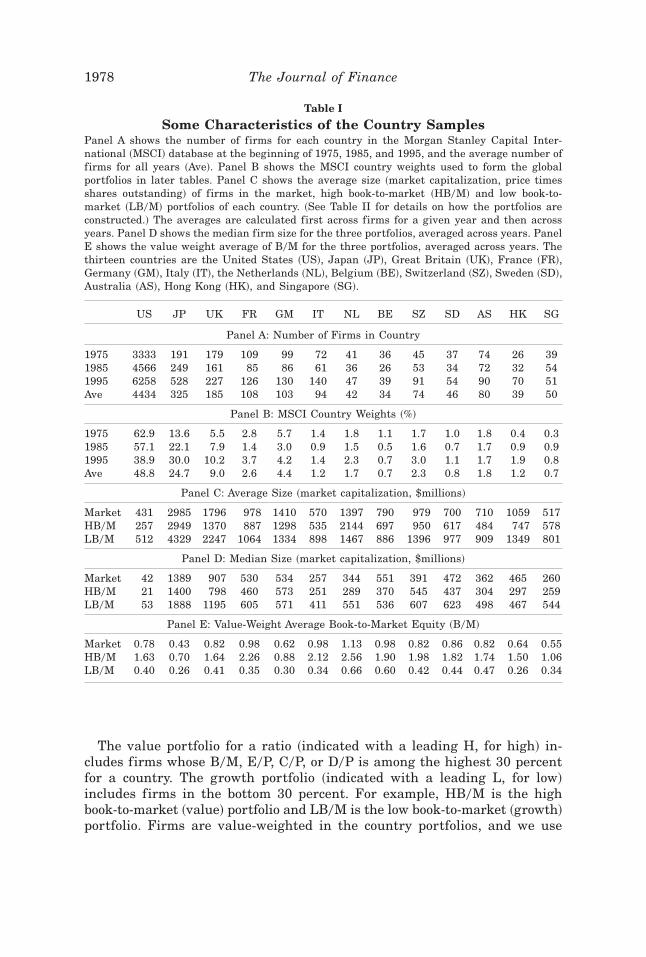
We study returns on market, value, and growth portfolios for the UnitedStates and twelve major EAFE ~Europe, Australia, and the Far East! coun-tries. The U.S. portfolios use all NYSE, AMEX, and Nasdaq stocks with therelevant CRSP and COMPUSTAT data. Most of the data for major marketsoutside the United States are from the electronic version of Morgan Stan-ley’s Capital International Perspectives ~MSCI!. The twelve countries we useare all those with MSCI accounting ratios ~B0M, E0P, C0P, and D0P! for atleast ten firms in each December from 1974 to 1994. We do not require thatthe same firms have data on all ratios. ~See Table II, below, for details onhow we construct the portfolios.!

The MSCI data have an important advantage. Other international data-bases often include only currently traded firms and so are subject to survi-vor bias. The MSCI database is just a compilation of the hard-copy issues ofMorgan Stanley’s Capital International Perspectives. It includes historicaldata for firms that disappear, but it does not include historical data fornewly added firms, so there is no backfilling problem. Thus, the data are

1976 The Journal of Finance

relatively free of survivor bias. Because the accounting data on MSCI arealso from Capital International Perspectives, their availability on the hard-copy publication date is clear-cut.

MSCI includes only a subset of the firms in any market, primarily thosein Morgan Stanley’s EAFE index or in the MSCI index for a country’s mar-ket. This means that most of the MSCI firms are large—in fact they accountfor the majority ~MSCI’s target is 80 percent! of a market’s invested wealth,so they provide a good description of the market’s performance. Preliminarytests we have done ~but do not show! confirm, however, that a database oflarge stocks does not allow meaningful tests for a size effect, such as thatfound by Banz ~1981! in U.S. returns, and that suggested by Heston, Rou-wenhorst, and Wessels ~1995! for international returns.

Table I summarizes our samples. The more complete U.S. sample ~fromCRSP and COMPUSTAT! always has at least ten times more firms than anyof the twelve EAFE countries. But because MSCI covers mostly large stocks,the median and average market capitalizations of the MSCI stocks are typ-ically several times those of the U.S. sample. ~Other features of the samplesreported in Table I are discussed later.!

Calculating returns from the MSCI data presents a problem. Stock pricesare available for the end of each month, but information about dividends islimited to the dividend yield, defined as the ratio of the trailing year ofdividends to the end-of-month stock price. The dividend yield allows accu-rate calculation of an annual return ~without intrayear reinvestment of div-idends!. Annual returns suffice for estimating expected returns, but tests ofasset pricing models ~which also require second moments! are hopelesslyimprecise unless returns for shorter intervals are used. To estimate monthlyreturns, we spread the annual dividend for a calendar year across all monthsof the year so that compounding the monthly returns reproduces the annualreturn. This approach maintains the integrity of average returns. But itassumes that the capital gain component of monthly returns, which is mea-sured accurately, reproduces the volatility and covariance structure of totalmonthly returns.

II. The Value Premium

Tables II and III summarize global and country returns for 1975 through1995 for value and growth portfolios formed on B0M, E0P, C0P, and D0P. Forthe twelve MSCI EAFE countries, the portfolios are formed at the end ofeach calendar year from 1974 to 1994, and returns are calculated for thefollowing year. ~Table II gives details.! We also form the U.S. portfolios atthe end of December of each year, using year-end CRSP stock prices andCOMPUSTAT accounting data for the most recent fiscal year. Because theavailability date for accounting data is less clear-cut for COMPUSTAT thanfor MSCI, we calculate returns on the U.S. portfolios beginning in July, sixmonths after portfolio formation ~as in Fama and French ~1996!!.

Value versus Growth: The International Evidence 1977

The value portfolio for a ratio ~indicated with a leading H, for high! in-cludes firms whose B0M, E0P, C0P, or D0P is among the highest 30 percentfor a country. The growth portfolio ~indicated with a leading L, for low!includes firms in the bottom 30 percent. For example, HB0M is the highbook-to-market ~value! portfolio and LB0M is the low book-to-market ~growth!portfolio. Firms are value-weighted in the country portfolios, and we use

Table I

Some Characteristics of the Country SamplesPanel A shows the number of firms for each country in the Morgan Stanley Capital Inter-national ~MSCI! database at the beginning of 1975, 1985, and 1995, and the average number offirms for all years ~Ave!. Panel B shows the MSCI country weights used to form the globalportfolios in later tables. Panel C shows the average size ~market capitalization, price timesshares outstanding! of firms in the market, high book-to-market ~HB0M! and low book-to-market ~LB0M! portfolios of each country. ~See Table II for details on how the portfolios areconstructed.! The averages are calculated first across firms for a given year and then acrossyears. Panel D shows the median firm size for the three portfolios, averaged across years. PanelE shows the value weight average of B0M for the three portfolios, averaged across years. Thethirteen countries are the United States ~US!, Japan ~JP!, Great Britain ~UK!, France ~FR!,Germany ~GM!, Italy ~IT!, the Netherlands ~NL!, Belgium ~BE!, Switzerland ~SZ!, Sweden ~SD!,Australia ~AS!, Hong Kong ~HK!, and Singapore ~SG!.

US JP UK FR GM IT NL BE SZ SD AS HK SG

Panel A: Number of Firms in Country

1975 3333 191 179 109 99 72 41 36 45 37 74 26 391985 4566 249 161 85 86 61 36 26 53 34 72 32 541995 6258 528 227 126 130 140 47 39 91 54 90 70 51Ave 4434 325 185 108 103 94 42 34 74 46 80 39 50

Panel B: MSCI Country Weights ~%!

1975 62.9 13.6 5.5 2.8 5.7 1.4 1.8 1.1 1.7 1.0 1.8 0.4 0.31985 57.1 22.1 7.9 1.4 3.0 0.9 1.5 0.5 1.6 0.7 1.7 0.9 0.91995 38.9 30.0 10.2 3.7 4.2 1.4 2.3 0.7 3.0 1.1 1.7 1.9 0.8Ave 48.8 24.7 9.0 2.6 4.4 1.2 1.7 0.7 2.3 0.8 1.8 1.2 0.7

Panel C: Average Size ~market capitalization, $millions!

Market 431 2985 1796 978 1410 570 1397 790 979 700 710 1059 517HB0M 257 2949 1370 887 1298 535 2144 697 950 617 484 747 578LB0M 512 4329 2247 1064 1334 898 1467 886 1396 977 909 1349 801

Panel D: Median Size ~market capitalization, $millions!

Market 42 1389 907 530 534 257 344 551 391 472 362 465 260HB0M 21 1400 798 460 573 251 289 370 545 437 304 297 259LB0M 53 1888 1195 605 571 411 551 536 607 623 498 467 544

Panel E: Value-Weight Average Book-to-Market Equity ~B0M!

Market 0.78 0.43 0.82 0.98 0.62 0.98 1.13 0.98 0.82 0.86 0.82 0.64 0.55HB0M 1.63 0.70 1.64 2.26 0.88 2.12 2.56 1.90 1.98 1.82 1.74 1.50 1.06LB0M 0.40 0.26 0.41 0.35 0.30 0.34 0.66 0.60 0.42 0.44 0.47 0.26 0.34


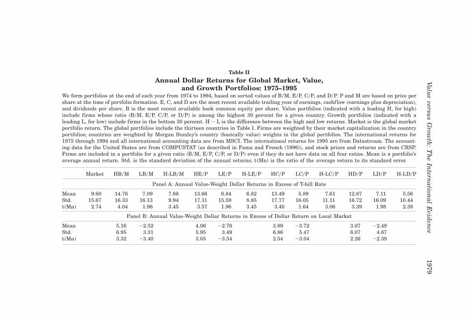
Table II

Annual Dollar Returns for Global Market, Value,and Growth Portfolios: 1975–1995

We form portfolios at the end of each year from 1974 to 1994, based on sorted values of B0M, E0P, C0P, and D0P. P and M are based on price pershare at the time of portfolio formation. E, C, and D are the most recent available trailing year of earnings, cashf low ~earnings plus depreciation!,and dividends per share. B is the most recent available book common equity per share. Value portfolios ~indicated with a leading H, for high!include firms whose ratio ~B0M, E0P, C0P, or D0P! is among the highest 30 percent for a given country. Growth portfolios ~indicated with aleading L, for low! include firms in the bottom 30 percent. H 2 L is the difference between the high and low returns. Market is the global marketportfolio return. The global portfolios include the thirteen countries in Table I. Firms are weighted by their market capitalization in the countryportfolios; countries are weighted by Morgan Stanley’s country ~basically value! weights in the global portfolios. The international returns for1975 through 1994 and all international accounting data are from MSCI. The international returns for 1995 are from Datastream. The account-ing data for the United States are from COMPUSTAT ~as described in Fama and French ~1996!!, and stock prices and returns are from CRSP.Firms are included in a portfolio for a given ratio ~B0M, E0P, C0P, or D0P! even if they do not have data on all four ratios. Mean is a portfolio’saverage annual return. Std. is the standard deviation of the annual returns; t~Mn! is the ratio of the average return to its standard error.

Market HB0M LB0M H-LB0M HE0P LE0P H-LE0P HC0P LC0P H-LC0P HD0P LD0P H-LD0P

Panel A: Annual Value-Weight Dollar Returns in Excess of T-bill Rate

Mean 9.60 14.76 7.09 7.68 13.66 6.84 6.82 13.49 5.89 7.61 12.67 7.11 5.56Std. 15.67 16.33 16.13 9.94 17.11 15.59 8.85 17.77 16.05 11.11 16.72 16.09 10.44t~Mn! 2.74 4.04 1.96 3.45 3.57 1.96 3.45 3.40 1.64 3.06 3.39 1.98 2.38

Panel B: Annual Value-Weight Dollar Returns in Excess of Dollar Return on Local Market

Mean 5.16 22.52 4.06 22.76 3.89 23.72 3.07 22.49Std. 6.95 3.31 5.95 3.49 6.86 5.47 6.07 4.67t~Mn! 3.32 23.40 3.05 23.54 2.54 23.04 2.26 22.38

Value

versus

Grow

th:

Th

eIn

ternation

alE

viden

ce1979

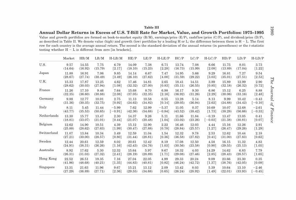
Table III

Annual Dollar Returns in Excess of U.S. T-Bill Rate for Market, Value, and Growth Portfolios: 1975–1995Value and growth portfolios are formed on book-to-market equity ~B0M!, earnings0price ~E0P!, cashf low0price ~C0P!, and dividend0price ~D0P!,as described in Table II. We denote value ~high! and growth ~low! portfolios by a leading H or L; the difference between them is H 2 L. The firstrow for each country is the average annual return. The second is the standard deviation of the annual returns ~in parentheses! or the t-statistictesting whether H 2 L is different from zero @in brackets#.

Market HB0M LB0M H-LB0M HE0P LE0P H-LE0P HC0P LC0P H-LC0P HD0P LD0P H-LD0P

U.S. 9.57 14.55 7.75 6.79 14.09 7.38 6.71 13.74 7.08 6.66 11.75 8.01 3.73~14.64! ~16.92! ~15.79! @2.17# ~18.10! ~15.23! @2.28# ~16.73! ~15.99! @2.08# ~13.89! ~17.04! @1.22#

Japan 11.88 16.91 7.06 9.85 14.14 6.67 7.47 14.95 5.66 9.29 16.81 7.27 9.54~28.67! ~27.74! ~30.49! @3.49# ~26.10! ~27.62! @4.00# ~31.59! ~29.22! @3.03# ~35.01! ~27.51! @2.53#

U.K. 15.33 17.87 13.25 4.62 17.46 14.81 2.65 18.41 14.51 3.89 15.89 12.99 2.90~28.62! ~30.03! ~27.94! @1.08# ~32.32! ~27.00! @0.83# ~35.11! ~26.55! @0.85# ~32.18! ~26.32! @0.72#

France 11.26 17.10 9.46 7.64 15.68 8.70 6.98 16.17 9.30 6.86 15.12 6.25 8.88~32.35! ~36.60! ~30.88! @2.08# ~37.05! ~32.35! @2.16# ~36.92! ~31.26! @2.29# ~30.06! ~33.16! @2.48#

Germany 9.88 12.77 10.01 2.75 11.13 10.58 0.55 13.28 5.14 8.13 9.99 10.42 20.43~31.36! ~30.35! ~32.75! @0.92# ~24.62! ~34.82! @0.14# ~29.05! ~26.94! @2.62# ~24.88! ~34.42! @20.10#

Italy 8.11 5.45 11.44 25.99 7.62 12.99 25.37 11.05 0.37 10.69 10.07 12.68 22.61~43.77! ~35.53! ~50.65! @20.91# ~42.36! ~54.68! @20.84# ~43.52! ~38.42! @1.73# ~38.28! ~56.66! @20.33#

Netherlands 13.30 15.77 13.47 2.30 14.37 9.26 5.11 11.66 11.84 20.19 13.47 13.05 0.41~18.81! ~33.07! ~21.01! @0.44# ~21.07! ~20.48! @1.04# ~33.02! ~23.26! @20.03# ~21.38! ~30.81! @0.07#

Belgium 12.62 14.90 10.51 4.39 15.12 12.90 2.22 16.46 12.03 4.44 15.16 12.26 2.91~25.88! ~28.62! ~27.63! @1.99# ~30.47! ~27.88! @0.78# ~28.84! ~25.57! @1.27# ~26.47! ~29.26! @1.29#

Switzerland 11.07 13.84 10.34 3.49 12.59 11.04 1.54 12.32 9.78 2.53 12.62 10.44 2.18~27.21! ~30.00! ~28.57! @0.80# ~31.44! ~28.81! @0.36# ~36.58! ~27.82! @0.41# ~31.00! ~27.83! @0.63#

Sweden 12.44 20.61 12.59 8.02 20.61 12.42 8.19 17.08 12.50 4.58 16.15 11.32 4.83~24.91! ~38.31! ~26.26! @1.16# ~42.43! ~24.76! @1.03# ~30.56! ~23.58! @0.90# ~29.55! ~25.13! @1.05#

Australia 8.92 17.62 5.30 12.32 15.64 5.97 9.67 18.32 4.03 14.29 14.62 6.83 7.79~26.31! ~31.03! ~27.32! @2.41# ~28.19! ~28.89! @1.71# ~29.08! ~27.46! @2.85# ~28.43! ~28.57! @1.65#

Hong Kong 22.52 26.51 19.35 7.16 27.04 22.05 4.99 29.33 20.24 9.09 23.66 23.30 0.35~41.96! ~48.68! ~40.21! @1.35# ~44.83! ~40.81! @0.82# ~46.24! ~42.72! @1.37# ~38.76! ~42.05! @0.09#

Singapore 13.31 21.63 11.96 9.67 15.21 13.12 2.09 13.42 8.03 5.39 10.64 13.10 22.46~27.29! ~36.89! ~27.71! @2.36# ~29.55! ~34.68! @0.65# ~26.24! ~28.92! @1.49# ~22.01! ~33.93! @20.45#

1980T

he

Jou

rnal

ofF

inan

ce

Morgan Stanley’s country ~basically total value of market! weights to con-struct global portfolios. The country weights at the beginning of 1975, 1985,and 1995 are in Table I.

Tables II and III are strong evidence of a consistent value premium ininternational returns. The average returns on the global value portfolios inTable II are 3.07 percent to 5.16 percent per year higher than the averagereturns on the global market portfolio, and the average returns on the globalvalue portfolios are 5.56 percent to 7.68 percent higher than the averagereturns on the corresponding global growth portfolios. Since the United Statesand Japan on average account for close to 75 percent of the global portfolios,the average returns for the global portfolios largely just confirm the resultsof Chan et al. ~1991!, Fama and French ~1992, 1996!, and Lakonishok et al.~1994!. Table III shows, however, that higher returns on value portfolios arealso the norm for other countries. When portfolios are formed on B0M, E0P,or C0P, twelve of the thirteen value-growth premiums are positive, and mostare more than four percent per year. Value premiums for individual coun-tries are a bit less consistent when portfolios are formed on dividend yield,but even here ten of thirteen are positive.

Table III says the value premium is pervasive. Thus, rather than beingunusual, the higher average returns on value stocks in the United States area local manifestation of a global phenomenon. Table III also shows that theU.S. value premium is not unusually large. For example, the U.S. book-to-market value premium is smaller than six of the other twelve B0M premi-ums. The results for other countries are out-of-sample relative to the earliertests for the United States and Japan, so clearly the value premium is notthe result of data mining.

Leaning on Foster, Smith, and Whaley ~1997!, a skeptic might argue thatthe correlation of returns across markets can cause similar chance patternsin average returns to show up in many markets. We shall see, however, thatthe correlations of the value premiums across countries are typically low.~The average for the B0M premiums is 0.09.! The simulations of Foster et al.~1997! then actually suggest that our results are rather good out-of-sampleevidence for a value premium.

The value premiums for individual countries in Table III are large in eco-nomic terms, but they are not typically large relative to their standard er-rors. This is testimony to the high volatility of the country returns. Themarket returns of many countries have standard deviations of approxi-mately 30 percent per year, about twice that of the global market portfolio inTable II. The most precise evidence that there is a value premium in inter-national returns comes from the diversified global portfolios ~Table II!. Thesmallest average spread between global value and growth returns, 5.56 per-cent per year for the D0P portfolios, is 2.38 standard errors from zero. Thevalue premiums for portfolios formed on B0M, E0P, and C0P ~7.68 percent,6.82 percent, and 7.61 percent per year! are more than three standard errorsfrom zero. We next examine whether the international value premium canbe viewed as compensation for risk.


III. A Risk Story for the Global Value Premiums

Researchers have identified several patterns in the cross section of inter-national stock returns. Heston et al. ~1995! find that equal-weight portfoliosof stocks tend to have higher average returns than value-weight portfolios intwelve European markets. They conclude that there is an international sizeeffect. Dumas and Solnik ~1995! find that exchange rate risks are priced instock returns around the world. Cho, Eun, and Senbet ~1986! and Korajczykand Viallet ~1989! find that APT factors ~identified by factor analysis! areimportant in international stock returns. Finally, Ferson and Harvey ~1993!present evidence that the loadings of country portfolios on international riskfactors vary through time.

In light of these results, a full description of expected stock returns aroundthe world would likely require a pricing model with several dimensions ofrisk and time-varying risk loadings. We take a more stripped-down ap-proach. We assume a world in which capital markets are integrated andinvestors are unconcerned with deviations from purchasing power parity. Wetest whether average returns are consistent with either an internationalCAPM or a two-factor ICAPM ~or APT! in which relative distress carries anexpected premium not captured by a stock’s sensitivity to the global marketreturn. Thus, we ignore other risk factors that might affect expected re-turns, and we do not allow for time-varying risk loadings. Fortunately, thetests suggest that, at least for the portfolios we examine, our simple ap-proach provides a reasonably adequate story for average returns.

We begin with asset pricing tests that attempt to explain the returns onthe global value and growth portfolios. We then use the same models toexplain the returns on the market, value, and growth portfolios of individualcountries.

A. The CAPM

Suppose the relevant model is an international CAPM. Thus, the globalmarket portfolio is mean-variance-efficient, and the dollar expected returnon any security or portfolio is fully explained by its loading ~univariate re-gression slope! on the dollar global market return, M. In the regression ofany portfolio’s excess return ~its dollar return, R, minus the return on a U.S.Treasury bill, F! on the excess market return,

R 2 F 5 a 1 b@M 2 F# 1 e, ~1!

the intercept should be statistically indistinguishable from zero.The estimates of equation ~1! in Table IV say that an international CAPM

cannot explain the average returns on global value and growth portfolios.The intercepts for the four value portfolios ~HB0M, HE0P, HC0P, and HD0P!are at least 29 basis points per month above zero, and the intercepts for thefour growth portfolios are at least 21 basis points per month below zero. All


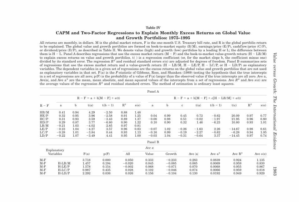
Table IV

CAPM and Two-Factor Regressions to Explain Monthly Excess Returns on Global Valueand Growth Portfolios: 1975–1995

All returns are monthly, in dollars. M is the global market return, F is the one-month U.S. Treasury bill rate, and R is the global portfolio returnto be explained. The global value and growth portfolios are formed on book-to-market equity ~B0M!, earnings0price ~E0P!, cashf low0price ~C0P!,or dividend0price ~D0P!, as described in Table II. We denote value ~high! and growth ~low! portfolios by a leading H or L; the difference betweenthem is H 2 L. Panel A describes regressions that use the excess market return ~M 2 F! and the book-to-market value-growth return ~H 2 LB0M!to explain excess returns on value and growth portfolios. t~ ! is a regression coefficient ~or, for the market slope b, the coefficient minus one!divided by its standard error. The regression R2 and residual standard errors s~e! are adjusted for degrees of freedom. Panel B summarizes setsof regressions that use the excess market return and a value-growth return ~H 2 LB0M, H 2 LE0P, H 2 LC0P, or H 2 LD0P! as explanatoryvariables. The dependent variables in a given set of regressions are the excess returns on the global value and growth portfolios that are not usedas explanatory variables in that set. F~a! is the F-statistic of Gibbons, Ross, and Shanken ~1989! testing the hypothesis that the true interceptsin a set of regressions are all zero; p~F! is the probability of a value of F~a! larger than the observed value if the true intercepts are all zero. Ave a,Ave|a|, and Ave a2 are the mean, mean absolute, and mean squared values of the intercepts from a set of regressions. Ave R2 and Ave s~e! arethe average values of the regression R2 and residual standard errors. The method of estimation is ordinary least squares.

Panel A

R 2 F 5 a 1 b@M 2 F# 1 e~t! R 2 F 5 a 1 b@M 2 F# 1 c@H 2 LB0M# 1 e~t!

R 2 F a b t~a! t~b 5 1! R2 s~e! a b c t~a! t~b 5 1! t~c! R2 s~e!

HB0M 0.41 0.94 4.29 22.50 0.88 1.48HE0P 0.32 0.95 3.96 22.58 0.91 1.25 0.04 0.99 0.45 0.72 20.62 20.09 0.97 0.77HC0P 0.31 0.93 3.59 23.43 0.89 1.37 20.00 0.98 0.51 20.02 21.97 21.95 0.96 0.80HD0P 0.29 0.87 3.77 26.80 0.90 1.22 0.10 0.90 0.32 1.46 26.23 10.80 0.93 1.01LB0M 20.21 1.03 24.02 2.85 0.97 0.81LE0P 20.23 1.04 24.27 3.57 0.96 0.83 20.07 1.02 20.26 21.63 2.26 214.67 0.98 0.61LC0P 20.28 1.01 23.84 0.44 0.93 1.13 20.16 0.99 20.19 22.27 20.62 26.28 0.94 1.05LD0P 20.22 1.07 23.49 4.41 0.95 1.00 20.03 1.04 20.31 20.64 3.37 214.45 0.97 0.74

Panel B

Ave aExplanatory

Variables F~a! p~F! All Value Growth Ave |a| Ave a2 Ave R2 Ave s~e!

M-F 3.718 0.000 0.050 0.333 20.233 0.283 0.0839 0.924 1.135M-F H-LB0M 1.457 0.194 20.020 0.045 20.085 0.065 0.0069 0.959 0.830M-F H-LE0P 1.578 0.154 20.002 0.068 20.071 0.070 0.0068 0.955 0.867M-F H-LC0P 0.987 0.435 0.028 0.102 20.046 0.074 0.0066 0.959 0.818M-F H-LD0P 2.292 0.036 0.026 0.156 20.104 0.130 0.0192 0.949 0.929

Value

versus

Grow

th:

Th

eIn

ternation

alE

viden

ce1983

the CAPM intercepts for the global value and growth portfolios are morethan 3.4 standard errors from zero. The GRS F-test ~Gibbons, Ross, andShanken ~1989!! of the hypothesis that the true intercepts are all zero re-jects with a high level of confidence ~ p-value 5 0.000!. In both statistical andpractical terms, the international CAPM is a poor model for global value andgrowth returns.

Why does the CAPM fail? If the CAPM is to explain the high returns onglobal value portfolios, they must have large slopes on the global marketportfolio. Similarly, if the CAPM is to explain the lower returns on globalgrowth portfolios, their market slopes must be less than one. In fact, thereverse is true. Table IV shows that the value portfolios’ market slopes areslightly less than one, and the growth portfolios’ slopes are slightly greaterthan one.

B. Two-Factor Regressions

Are the premiums on global value portfolios and the discounts on globalgrowth portfolios compensation for risk? In an international two-factor ~one-state-variable! ICAPM, expected returns are explained by the loadings ofsecurities and portfolios on the global market return and the return on anyother global two-factor MMV ~multifactor-minimum-variance! portfolio ~Fama~1996!!. ~Two-factor MMV portfolios have the smallest possible return vari-ances, given their expected returns and loadings on the state variable whosepricing is not captured by the CAPM.! Alternatively, the market return andthe difference between the returns on two MMV portfolios can be used toexplain expected returns.

We assume that the global high and low book-to-market portfolios, HB0Mand LB0M, are two-factor MMV, so the difference between their returns,H2LB0M, can be the second explanatory return in a one-state-variable ICAPM.The model then predicts that the intercept in the time-series regression,

R 2 F 5 a 1 b@M 2 F# 1 c@H 2 LB0M # 1 e, ~2!

is zero for all the portfolios whose returns, R, we seek to explain. We useH 2 LB0M, rather than HB0M 2 F or LB0M 2 F, because the correlation ofH 2 LB0M with M 2 F is only 20.17. The low correlation makes the slopesin equation ~2! easy to interpret. Moreover, H 2 LB0M is an internationalversion of HML, the distress factor in the three-factor model for U.S. stockreturns in Fama and French ~1993!.

Table IV says that the two-factor model ~2! provides better descriptionsof the returns on global value and growth portfolios formed on E0P, C0P,and D0P than does the CAPM. The average intercept for the global valueportfolios drops from 33.3 basis points per month in the CAPM regression~equation ~1!! to 4.5 basis points per month in the two-factor regression~equation ~2!!. Similarly, the average intercept for the global growth port-


folios rises from 223.3 basis points per month in equation ~1! to 28.5 basispoints in equation ~2!. The GRS test of the hypothesis that the interceptsare zero also favors equation ~2!. The F-statistic testing whether all ~valueand growth! intercepts are zero drops from 3.72 ~ p-value 5 0.000! in theCAPM regressions to 1.46 ~ p-value 5 0.194! in the two-factor regressions.

Why do the two-factor regressions produce better descriptions of globalvalue and growth returns? The two-factor regressions and the CAPM re-gressions produce similar market slopes. Thus the improvements must comefrom the H 2 LB0M slopes. Table IV confirms that these slopes are atleast ten standard errors above zero for the global value portfolios formedon E0P, C0P, and D0P, and they are at least six standard errors below zerofor the growth portfolios. Since the average H 2 LB0M return is positive,the positive H 2 LB0M slopes for the global value portfolios are consistentwith their high average returns, and the negative slopes for the growthportfolios are in line with their low average returns. Moreover, the successof the two-factor regressions in describing the returns on the global valueand growth portfolios says that different approaches to measuring valueand growth—specifically, portfolios formed on B0M, E0P, C0P, and D0P—produce premiums and discounts that can all be described as compensationfor a single common risk. In other words, global value-growth premiums,however measured, are consistent with a one-state variable ICAPM ~or atwo-factor APT!.

Table IV also shows that alternative measures of the value-growth pre-mium are largely interchangeable as the second explanatory return in equa-tion ~2!. Substituting H 2 LE0P or H 2 LC0P for H 2 LB0M produces similaraverage absolute intercepts, average squared intercepts, and GRS F-testsfor the global value and growth portfolios that are not used as explanatoryreturns. In results not shown, we also obtain excellent explanations of av-erage returns when we use the excess return on a single global value orgrowth portfolio ~e.g., HB0M 2 F or LB0M 2 F! as the second explanatoryreturn. All this is consistent with one-state-variable ICAPM pricing of globalvalue and growth portfolios, and with the hypothesis that, like the globalmarket portfolio, different global value and growth portfolios are close totwo-factor MMV.

One can argue that the global regressions do not provide a convincing testof a risk story for the international value premium. The four sorting vari-ables ~B0M, E0P, C0P, and D0P! are all versions of the inverted stock price,10P, so different global value ~or growth! portfolios have many stocks incommon. But the portfolios are far from identical. The squared correlationsbetween the four global value-growth returns ~proportions of variance ex-plained! range from only 0.37 to 0.67. Thus, although a reasonable suspicionremains, there is no guarantee that the average returns on different valueand growth portfolios will be described by their sensitivities to a single com-mon risk. Moreover, the properties of the global value premium examinednext and the extension of the asset pricing tests to country portfolios inSection IV lend additional support to a risk story.


C. Is the Global Value Premium Too Large?

MacKinlay ~1995! argues that the value premium in U.S. returns is toolarge to be explained by rational asset pricing. Lakonishok et al. ~1994! andHaugen ~1995! go a step further and argue that the U.S. value premium isclose to an arbitrage opportunity. Fama and French ~1996, especiallyTable XI! disagree.

Is the international value premium too large? The global market premiumis a good benchmark for judging the global value premiums. The mean andstandard deviation of the market premium ~M 2 F! in Table II are 9.60 percentand 15.67 percent per year. The average value-growth premiums are smaller,ranging from 5.56 percent per year when we sort on D0P to 7.68 percent peryear for B0M, but their standard deviations are also smaller, between 8.85 per-cent and 11.11 percent per year. The four t-statistics for the value-growth pre-miums, 2.38 to 3.45, bracket the t-statistic for the market premium, 2.74. Weconclude that the value-growth premiums are no more suspicious than the mar-ket premium. At a minimum, the large standard deviations of the value-growth premiums say that they are not arbitrage opportunities.

IV. Regression Tests for Country Returns

Since the global portfolios are highly diversified, they provide sharp per-spective on the CAPM’s inability to explain the international value pre-mium, and on the improvements provided by a two-factor model. In contrast,portfolios restricted to individual countries are less diversified and theirreturns have large idiosyncratic components ~e.g., Harvey ~1991!!. As a re-sult, asset pricing tests on country portfolios are noisier than tests on globalportfolios. But the country portfolios have an advantage. Because most ofthe country portfolios are small fractions of the global portfolios ~ Table I!,and because all have large idiosyncratic components, there is no reason tothink we induce a linear relation between average return and risk loadingsby the way we construct the explanatory portfolios. Thus, the country port-folios leave plenty of room for asset pricing models to fail.

A. The CAPM versus a Two-Factor Model

In an international CAPM, all expected returns are explained by slopes onthe global market return. Table V shows estimates of the CAPM time-seriesregression ~equation ~1!! that attempt to explain the returns on three sepa-rate sets of country portfolios that include, respectively, the market, highbook-to-market ~HB0M!, and low book-to-market ~LB0M! portfolios of ourthirteen countries. We group country portfolios by type ~rather than doingjoint tests on all portfolios and countries! to have some hope of power informal asset pricing tests.

Like Solnik ~1974!, Harvey ~1991!, and others, we find little evidence againstthe international CAPM as a model for the returns on the market portfoliosof countries. The GRS test of the hypothesis that all the intercepts in the


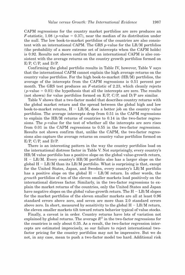
CAPM regressions for the country market portfolios are zero produces anF-statistic, 1.08 ~ p-value 5 0.37!, near the median of its distribution underthe null. The low book-to-market portfolios of the countries are also consis-tent with an international CAPM. The GRS p-value for the LB0M portfolios~the probability of a more extreme set of intercepts when the CAPM holds!is 0.92. Results not shown confirm that an international CAPM is also con-sistent with the average returns on the country growth portfolios formed onE0P, C0P, and D0P.

Confirming the global portfolio results in Table IV, however, Table V saysthat the international CAPM cannot explain the high average returns on thecountry value portfolios. For the high book-to-market ~HB0M! portfolios, theaverage of the intercepts from the CAPM regressions is 0.51 percent permonth. The GRS test produces an F-statistic of 2.23, which cleanly rejects~ p-value 5 0.01! the hypothesis that all the intercepts are zero. The results~not shown! for value portfolios formed on E0P, C0P, and D0P are similar.

Table V shows that a two-factor model that describes country returns withthe global market return and the spread between the global high and lowbook-to-market returns, H 2 LB0M, does a better job on the country valueportfolios. The average intercepts drop from 0.51 in the CAPM regressionsto explain the HB0M returns of countries to 0.14 in the two-factor regres-sions. The p-value for the test of whether all the intercepts are zero risesfrom 0.01 in the CAPM regressions to 0.55 in the two-factor regressions.Results not shown confirm that, unlike the CAPM, the two-factor regres-sions also capture the average returns on country value portfolios formed onE0P, C0P, and D0P.

There is an interesting pattern in the way the country portfolios load onthe international distress factor in Table V. Not surprisingly, every country’sHB0M value portfolio has a positive slope on the global value-growth return,H 2 LB0M. Every country’s HB0M portfolio also has a larger slope on theglobal H 2 LB0M than its LB0M portfolio. What is surprising is that, exceptfor the United States, Japan, and Sweden, every country’s LB0M portfoliohas a positive slope on the global H 2 LB0M return. In other words, thegrowth portfolios of ten of the eleven smaller markets load positively on theinternational distress factor. Similarly, in the two-factor regressions to ex-plain the market returns of the countries, only the United States and Japanhave negative slopes on the global value-growth return. The H 2 LB0M slopesfor the market portfolios of the eleven smaller markets are all at least 0.96standard errors above zero, and seven are more than 2.0 standard errorsabove zero. In short, measured by sensitivity to the global H 2 LB0M return,the eleven smaller markets tilt toward return behavior typical of value stocks.

Finally, a caveat is in order. Country returns have lots of variation notexplained by global returns. The average R2 in the two-factor regressions forthe countries is only about 0.35. As a result, the two-factor regression inter-cepts are estimated imprecisely, so our failure to reject international two-factor pricing for the country portfolios may not be impressive. But we donot, in any case, mean to push a two-factor model too hard. Additional risk


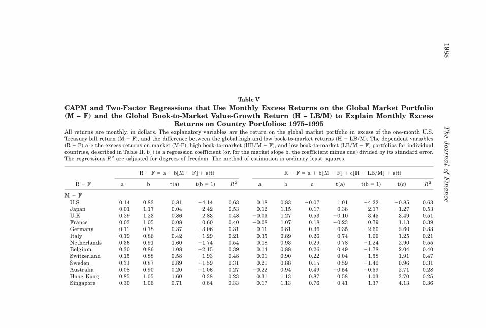
Table V

CAPM and Two-Factor Regressions that Use Monthly Excess Returns on the Global Market Portfolio(M − F) and the Global Book-to-Market Value-Growth Return (H − LB/M) to Explain Monthly Excess

Returns on Country Portfolios: 1975–1995All returns are monthly, in dollars. The explanatory variables are the return on the global market portfolio in excess of the one-month U.S.Treasury bill return ~M 2 F!, and the difference between the global high and low book-to-market returns ~H 2 LB0M!. The dependent variables~R 2 F! are the excess returns on market ~M-F!, high book-to-market ~HB0M 2 F!, and low book-to-market ~LB0M 2 F! portfolios for individualcountries, described in Table II. t~ ! is a regression coefficient ~or, for the market slope b, the coefficient minus one! divided by its standard error.The regressions R2 are adjusted for degrees of freedom. The method of estimation is ordinary least squares.

R 2 F 5 a 1 b@M 2 F# 1 e~t! R 2 F 5 a 1 b@M 2 F# 1 c@H 2 LB0M# 1 e~t!

R 2 F a b t~a! t~b 5 1! R2 a b c t~a! t~b 5 1! t~c! R2

M 2 FU.S. 0.14 0.83 0.81 24.14 0.63 0.18 0.83 20.07 1.01 24.22 20.85 0.63Japan 0.01 1.17 0.04 2.42 0.53 0.12 1.15 20.17 0.38 2.17 21.27 0.53U.K. 0.29 1.23 0.86 2.83 0.48 20.03 1.27 0.53 20.10 3.45 3.49 0.51France 0.03 1.05 0.08 0.60 0.40 20.08 1.07 0.18 20.23 0.79 1.13 0.39Germany 0.11 0.78 0.37 23.06 0.31 20.11 0.81 0.36 20.35 22.60 2.60 0.33Italy 20.19 0.86 20.42 21.29 0.21 20.35 0.89 0.26 20.74 21.06 1.25 0.21Netherlands 0.36 0.91 1.60 21.74 0.54 0.18 0.93 0.29 0.78 21.24 2.90 0.55Belgium 0.30 0.86 1.08 22.15 0.39 0.14 0.88 0.26 0.49 21.78 2.04 0.40Switzerland 0.15 0.88 0.58 21.93 0.48 0.01 0.90 0.22 0.04 21.58 1.91 0.47Sweden 0.31 0.87 0.89 21.59 0.31 0.21 0.88 0.15 0.59 21.40 0.96 0.31Australia 0.08 0.90 0.20 21.06 0.27 20.22 0.94 0.49 20.54 20.59 2.71 0.28Hong Kong 0.85 1.05 1.60 0.38 0.23 0.31 1.13 0.87 0.58 1.03 3.70 0.25Singapore 0.30 1.06 0.71 0.64 0.33 20.17 1.13 0.76 20.41 1.37 4.13 0.36

1988T

he

Jou

rnal

ofF

inan

ce

HB0M 2 FU.S. 0.52 0.77 2.67 24.90 0.53 0.15 0.83 0.60 0.84 24.04 7.38 0.61Japan 0.45 1.06 1.48 0.82 0.46 0.10 1.11 0.57 0.34 1.57 4.22 0.50U.K. 0.46 1.25 1.24 2.86 0.45 20.10 1.33 0.91 20.28 3.98 5.72 0.51France 0.43 1.06 1.05 0.60 0.32 0.11 1.10 0.51 0.27 1.09 2.80 0.34Germany 0.34 0.78 1.09 23.03 0.30 0.04 0.82 0.48 0.14 22.45 3.46 0.33Italy 20.22 0.83 20.44 21.41 0.16 20.38 0.86 0.26 20.74 21.19 1.15 0.16Netherlands 0.36 0.99 1.07 20.16 0.38 20.05 1.05 0.66 20.14 0.61 4.47 0.42Belgium 0.47 0.88 1.30 21.41 0.30 0.21 0.92 0.42 0.57 20.96 2.58 0.31Switzerland 0.35 0.87 1.21 21.84 0.39 0.04 0.92 0.50 0.14 21.19 3.88 0.43Sweden 0.80 0.89 1.67 20.98 0.20 0.46 0.94 0.56 0.93 20.53 2.58 0.21Australia 0.67 0.84 1.68 21.66 0.24 0.31 0.90 0.59 0.76 21.10 3.28 0.27Hong Kong 1.09 1.07 1.73 0.45 0.17 0.48 1.16 0.99 0.76 1.06 3.51 0.20Singapore 0.85 1.09 1.54 0.73 0.22 0.33 1.17 0.83 0.60 1.32 3.39 0.25

LB0M 2 FU.S. 20.02 0.88 20.09 22.60 0.58 0.23 0.84 20.40 1.13 23.43 24.51 0.61Japan 20.37 1.21 21.12 2.68 0.49 0.03 1.15 20.64 0.08 1.97 24.42 0.52U.K. 0.16 1.21 0.45 2.50 0.44 20.04 1.24 0.33 20.11 2.83 2.01 0.45France 20.07 1.01 20.19 0.18 0.37 20.13 1.02 0.10 20.35 0.28 0.61 0.37Germany 0.11 0.79 0.34 22.72 0.28 20.04 0.81 0.24 20.11 22.41 1.59 0.29Italy 20.05 0.85 20.10 21.37 0.20 20.20 0.88 0.24 20.42 21.15 1.19 0.20Netherlands 0.39 0.89 1.51 21.87 0.46 0.35 0.89 0.07 1.29 21.74 0.59 0.46Belgium 0.13 0.88 0.44 21.78 0.40 20.02 0.90 0.24 20.07 21.45 1.83 0.40Switzerland 0.08 0.88 0.29 21.87 0.43 0.01 0.89 0.11 0.04 21.69 0.88 0.43Sweden 0.28 0.88 0.85 21.53 0.34 0.32 0.87 20.07 0.94 21.59 20.45 0.34Australia 20.18 0.97 20.40 20.31 0.24 20.43 1.00 0.41 20.92 0.03 1.97 0.25Hong Kong 0.64 0.98 1.24 20.14 0.20 0.06 1.07 0.93 0.12 0.56 4.08 0.25Singapore 0.24 0.98 0.59 20.17 0.30 20.08 1.03 0.52 20.19 0.32 2.84 0.32

Value

versus

Grow

th:

Th

eIn

ternation

alE

viden

ce1989

factors are likely to be necessary to describe average returns when, for ex-ample, the tests are extended to small stocks. Like the more precise tests onthe global portfolios in Table IV, however, the tests on the country portfoliosin Table V do allow us to conclude that the addition of an internationaldistress factor provides a substantially better explanation of value portfolioreturns than an international CAPM.

B. Global Risks in Country Returns

The hypothesis that an international CAPM or ICAPM explains expectedreturns around the world does not require security returns to be correlatedacross countries. International asset pricing just says that the expected re-turns on assets are determined by their covariances with the global marketreturn ~CAPM and ICAPM! and the returns on global MMV portfolios neededto capture the effects of priced state variables ~ICAPM!. But covarianceswith these global returns ~and the variances of the global returns them-selves! may just result from the variances and covariances of asset returnswithin markets; that is, covariances between the asset returns of differentcountries may be zero.1 Still, it is interesting to ask whether the global mar-ket and distress risks that seem to explain country returns arise in partfrom covariances of returns across countries.

For direct evidence on the local and international components of globalportfolio returns, we decompose the variances of the global M 2 F and H 2LB0M returns into country return variances and the covariances of returnsacross countries,

Var~Rglobal! 5 (i

wi2 Var~Ri ! 1 (

i(jÞi

wi wj Cov~Ri , Rj !, ~3!

where wi is the weight of country i in the global portfolio and Ri is the returnfor the portfolio of country i. If there were no common component in returnsacross countries, the covariances in equation ~3! would contribute nothing tothe global variance. At the other extreme, with perfect correlation of returnsacross countries, the contribution of the covariances depends on countryweights and variances. Using the average country weights for 1975 through1995, country covariances would then account for about 75 percent of thevariances of the global M 2 F and H 2 LB0M returns. In fact, internationalcomponents ~the covariances in equation ~3!!, are 52 percent of the varianceof the global M 2 F return, and 19 percent of the variance of the global H 2LB0M return. Thus, although country-specific variances account for 81 per-

1 A similar argument implies that excluding left-hand-side country returns from right-hand-side global returns in regressions ~1! and ~2! ~an approach often advocated to avoid inducing aspurious relation between average return and risk! would corrupt the estimates of risk loadingsin tests for international asset pricing.


cent of the variance of the global H 2 LB0M return, both the global marketreturn and the global value-growth return contain important internationalcomponents.

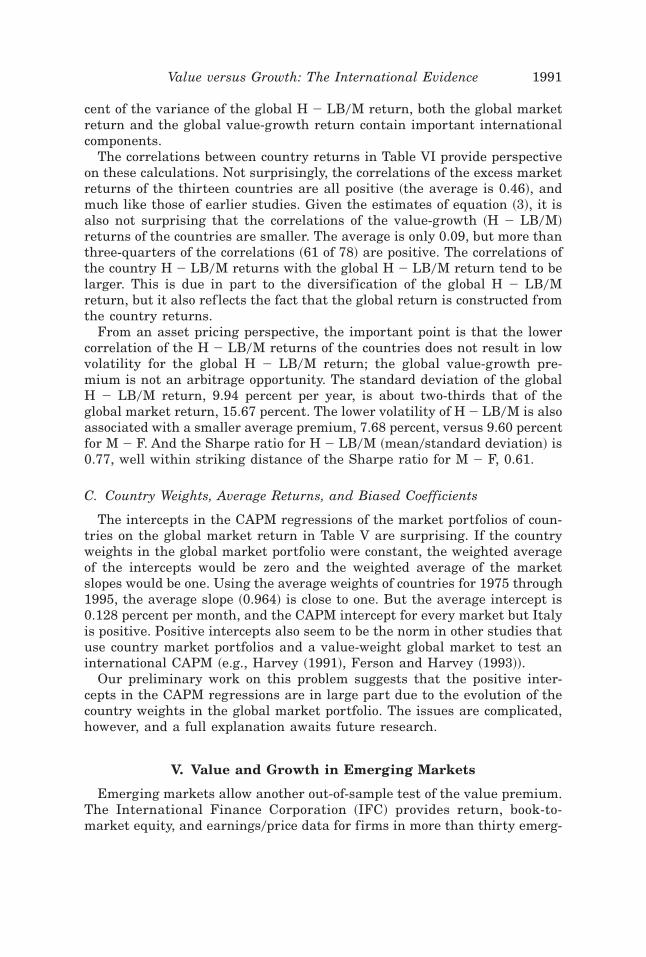
The correlations between country returns in Table VI provide perspectiveon these calculations. Not surprisingly, the correlations of the excess marketreturns of the thirteen countries are all positive ~the average is 0.46!, andmuch like those of earlier studies. Given the estimates of equation ~3!, it isalso not surprising that the correlations of the value-growth ~H 2 LB0M!returns of the countries are smaller. The average is only 0.09, but more thanthree-quarters of the correlations ~61 of 78! are positive. The correlations ofthe country H 2 LB0M returns with the global H 2 LB0M return tend to belarger. This is due in part to the diversification of the global H 2 LB0Mreturn, but it also ref lects the fact that the global return is constructed fromthe country returns.

From an asset pricing perspective, the important point is that the lowercorrelation of the H 2 LB0M returns of the countries does not result in lowvolatility for the global H 2 LB0M return; the global value-growth pre-mium is not an arbitrage opportunity. The standard deviation of the globalH 2 LB0M return, 9.94 percent per year, is about two-thirds that of theglobal market return, 15.67 percent. The lower volatility of H 2 LB0M is alsoassociated with a smaller average premium, 7.68 percent, versus 9.60 percentfor M 2 F. And the Sharpe ratio for H 2 LB0M ~mean0standard deviation! is0.77, well within striking distance of the Sharpe ratio for M 2 F, 0.61.

C. Country Weights, Average Returns, and Biased Coefficients

The intercepts in the CAPM regressions of the market portfolios of coun-tries on the global market return in Table V are surprising. If the countryweights in the global market portfolio were constant, the weighted averageof the intercepts would be zero and the weighted average of the marketslopes would be one. Using the average weights of countries for 1975 through1995, the average slope ~0.964! is close to one. But the average intercept is0.128 percent per month, and the CAPM intercept for every market but Italyis positive. Positive intercepts also seem to be the norm in other studies thatuse country market portfolios and a value-weight global market to test aninternational CAPM ~e.g., Harvey ~1991!, Ferson and Harvey ~1993!!.

Our preliminary work on this problem suggests that the positive inter-cepts in the CAPM regressions are in large part due to the evolution of thecountry weights in the global market portfolio. The issues are complicated,however, and a full explanation awaits future research.

V. Value and Growth in Emerging Markets

Emerging markets allow another out-of-sample test of the value premium.The International Finance Corporation ~IFC! provides return, book-to-market equity, and earnings0price data for firms in more than thirty emerg-


Table VI

Correlations of Excess Returns on Country Market Portfolios, M − F, and ofCountry Book-to-Market Value-Growth Returns, H − LB/M: 1975–1995

All returns are monthly, in dollars. M is a country’s market return, F is the one-month U.S. Treasury bill return, and H 2 LB0M is the differencebetween the returns on a country’s high and low book-to-market portfolios, as described in Table II. Global is the global M 2 F or H 2 LB0M return.

Global US JP UK FR GM IT NL BE SZ SD AU HK

Panel A: Correlations of Excess Market Returns, M 2 F

U.S. 0.80Japan 0.73 0.24U.K. 0.70 0.51 0.37France 0.63 0.44 0.42 0.54Germany 0.56 0.35 0.38 0.46 0.58Italy 0.46 0.23 0.40 0.39 0.44 0.39Neth. 0.73 0.58 0.42 0.65 0.58 0.71 0.36Belgium 0.63 0.42 0.44 0.54 0.65 0.67 0.39 0.69Switz. 0.68 0.49 0.44 0.59 0.59 0.72 0.36 0.74 0.66Sweden 0.56 0.39 0.41 0.42 0.34 0.41 0.34 0.47 0.41 0.48Australia 0.52 0.44 0.27 0.48 0.36 0.28 0.24 0.41 0.31 0.41 0.41H.K. 0.47 0.37 0.24 0.47 0.32 0.36 0.30 0.51 0.34 0.43 0.38 0.42Singapore 0.56 0.49 0.31 0.56 0.32 0.33 0.26 0.49 0.38 0.43 0.39 0.44 0.57

Panel B: Correlations of Book-to-Market Value-Growth Returns, H 2 LB0M

U.S. 0.77Japan 0.62 0.06U.K. 0.36 0.24 0.09France 0.21 0.13 0.03 0.27Germany 0.17 0.18 20.08 20.00 0.04Italy 0.01 20.05 0.02 0.03 0.01 0.01Neth. 0.24 0.10 0.14 0.21 0.20 0.16 20.02Belgium 0.09 0.04 0.04 0.07 0.09 20.06 0.08 0.16Switz. 0.24 0.14 0.10 0.08 0.15 0.22 0.05 0.11 0.10Sweden 0.23 0.18 0.08 0.16 0.22 0.13 0.04 0.23 0.06 0.15Australia 0.10 0.14 20.08 0.11 0.00 0.12 20.03 0.07 0.06 0.06 0.09Hong Kong 0.01 20.01 20.04 20.00 0.05 0.09 0.13 0.00 0.00 0.06 0.08 20.00Singapore 0.11 0.02 0.09 0.00 20.03 0.08 20.07 0.14 20.17 20.02 0.03 20.11 20.05

1992T

he

Jou

rnal

ofF

inan

ce

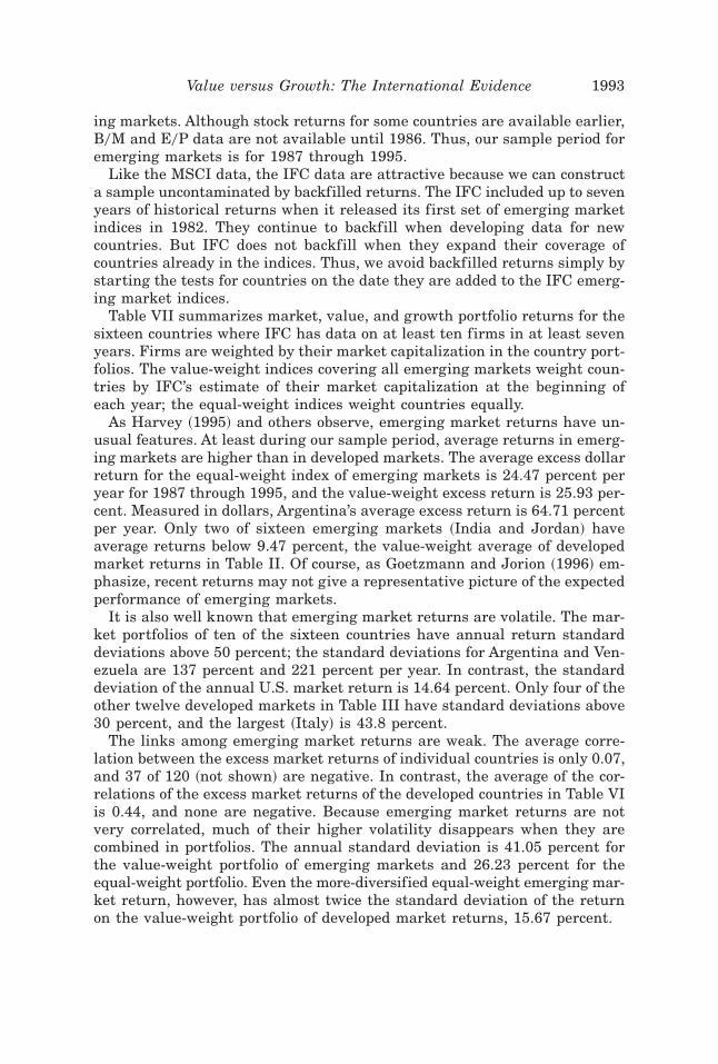
ing markets. Although stock returns for some countries are available earlier,B0M and E0P data are not available until 1986. Thus, our sample period foremerging markets is for 1987 through 1995.

Like the MSCI data, the IFC data are attractive because we can constructa sample uncontaminated by backfilled returns. The IFC included up to sevenyears of historical returns when it released its first set of emerging marketindices in 1982. They continue to backfill when developing data for newcountries. But IFC does not backfill when they expand their coverage ofcountries already in the indices. Thus, we avoid backfilled returns simply bystarting the tests for countries on the date they are added to the IFC emerg-ing market indices.

Table VII summarizes market, value, and growth portfolio returns for thesixteen countries where IFC has data on at least ten firms in at least sevenyears. Firms are weighted by their market capitalization in the country port-folios. The value-weight indices covering all emerging markets weight coun-tries by IFC’s estimate of their market capitalization at the beginning ofeach year; the equal-weight indices weight countries equally.

As Harvey ~1995! and others observe, emerging market returns have un-usual features. At least during our sample period, average returns in emerg-ing markets are higher than in developed markets. The average excess dollarreturn for the equal-weight index of emerging markets is 24.47 percent peryear for 1987 through 1995, and the value-weight excess return is 25.93 per-cent. Measured in dollars, Argentina’s average excess return is 64.71 percentper year. Only two of sixteen emerging markets ~India and Jordan! haveaverage returns below 9.47 percent, the value-weight average of developedmarket returns in Table II. Of course, as Goetzmann and Jorion ~1996! em-phasize, recent returns may not give a representative picture of the expectedperformance of emerging markets.

It is also well known that emerging market returns are volatile. The mar-ket portfolios of ten of the sixteen countries have annual return standarddeviations above 50 percent; the standard deviations for Argentina and Ven-ezuela are 137 percent and 221 percent per year. In contrast, the standarddeviation of the annual U.S. market return is 14.64 percent. Only four of theother twelve developed markets in Table III have standard deviations above30 percent, and the largest ~Italy! is 43.8 percent.

The links among emerging market returns are weak. The average corre-lation between the excess market returns of individual countries is only 0.07,and 37 of 120 ~not shown! are negative. In contrast, the average of the cor-relations of the excess market returns of the developed countries in Table VIis 0.44, and none are negative. Because emerging market returns are notvery correlated, much of their higher volatility disappears when they arecombined in portfolios. The annual standard deviation is 41.05 percent forthe value-weight portfolio of emerging markets and 26.23 percent for theequal-weight portfolio. Even the more-diversified equal-weight emerging mar-ket return, however, has almost twice the standard deviation of the returnon the value-weight portfolio of developed market returns, 15.67 percent.


Table VII

Annual Dollar Returns in Excess of U.S. T-Bill Rates for Emerging MarketsThe emerging market data are from the IFC. Value and growth portfolios using book-to-market equity ~B0M! and earnings0price ~E0P! as inTable II. The Small and Big portfolios are formed on market capitalization, in an analogous manner. We denote value ~high! and growth ~low!portfolios by a leading H or L; the difference between them is H 2 L. S 2 B is the difference between the Small and Big portfolios. Countries areincluded in the table ~and indices! if the IFC database includes at least ten firms with positive book equity in at least seven years. Countries arenot included in a year’s B0M ~or E0P! portfolios if the IFC has fewer than ten firms with positive book equity ~or earnings! at the end of theprevious year. Thus, the B0M and E0P portfolio returns for Chile do not include 1988, and the E0P portfolio returns for Jordan do not include1987 and 1988. The VW indices weight countries by the IFC’s estimate of their total market capitalization. The EW indices weight countriesequally. The first row for each country or index is the average annual return. The second is the standard deviation of the annual returns ~inparentheses! or the t-statistic testing whether H 2 L or S 2 B is different from zero @in brackets#.

Market HB0M LB0M H 2 LB0M HE0P LE0P H 2 LE0P Small Big S 2 B

VW indices 25.93 39.77 22.86 16.91 29.52 25.49 4.04 39.78 24.89 14.891987–1995 ~41.05! ~49.88! ~35.40! @3.06# ~47.36! ~38.03! @0.58# ~52.42! ~39.87! @1.69#

EW indices 24.47 33.21 19.07 14.13 29.60 19.18 10.43 32.01 23.32 8.701987–1995 ~26.23! ~31.43! ~21.48! @3.01# ~14.09! ~34.32! @1.86# ~26.41! ~26.32! @1.98#

Argentina 64.71 38.27 74.74 236.47 101.33 62.72 38.61 66.60 62.54 4.061987–1995 ~137.06! ~136.13! ~150.08! @21.39# ~256.37! ~152.04! @1.03# ~175.97! ~130.50! @0.11#

Brazil 34.99 87.67 13.95 73.72 39.41 33.82 5.59 45.02 33.08 11.941987–1995 ~79.15! ~128.57! ~53.95! @2.33# ~96.26! ~77.45! @0.20# ~99.84! ~77.36! @0.57#

Chile 35.58 48.07 32.86 15.21 39.17 29.57 9.60 45.02 36.33 8.691987–1995 ~30.03! ~49.93! ~41.68! @1.12# ~36.56! ~48.21! @1.23# ~39.67! ~30.50! @0.98#

Colombia 33.16 4.90 22.37 217.47 21.68 31.97 210.29 11.08 31.61 220.541988–1995 ~65.85! ~51.10! ~50.07! @22.18# ~85.79! ~53.69! @20.56# ~45.97! ~62.71! @21.98#

Greece 19.92 22.36 19.73 2.63 17.44 15.08 2.36 9.49 21.06 211.571989–1995 ~47.49! ~53.33! ~45.08! @0.39# ~51.51! ~53.01! @0.19# ~39.61! ~48.27! @21.04#

1994T

he

Jou

rnal

ofF

inan

ce

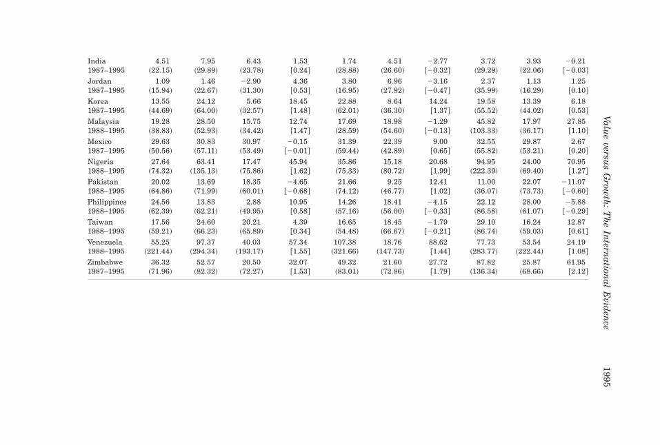
India 4.51 7.95 6.43 1.53 1.74 4.51 22.77 3.72 3.93 20.211987–1995 ~22.15! ~29.89! ~23.78! @0.24# ~28.88! ~26.60! @20.32# ~29.29! ~22.06! @20.03#

Jordan 1.09 1.46 22.90 4.36 3.80 6.96 23.16 2.37 1.13 1.251987–1995 ~15.94! ~22.67! ~31.30! @0.53# ~16.95! ~27.92! @20.47# ~35.99! ~16.29! @0.10#

Korea 13.55 24.12 5.66 18.45 22.88 8.64 14.24 19.58 13.39 6.181987–1995 ~44.69! ~64.00! ~32.57! @1.48# ~62.01! ~36.30! @1.37# ~55.52! ~44.02! @0.53#

Malaysia 19.28 28.50 15.75 12.74 17.69 18.98 21.29 45.82 17.97 27.851988–1995 ~38.83! ~52.93! ~34.42! @1.47# ~28.59! ~54.60! @20.13# ~103.33! ~36.17! @1.10#

Mexico 29.63 30.83 30.97 20.15 31.39 22.39 9.00 32.55 29.87 2.671987–1995 ~50.56! ~57.11! ~53.49! @20.01# ~59.44! ~42.89! @0.65# ~55.82! ~53.21! @0.20#

Nigeria 27.64 63.41 17.47 45.94 35.86 15.18 20.68 94.95 24.00 70.951988–1995 ~74.32! ~135.13! ~75.86! @1.62# ~75.33! ~80.72! @1.99# ~222.39! ~69.40! @1.27#

Pakistan 20.02 13.69 18.35 24.65 21.66 9.25 12.41 11.00 22.07 211.071988–1995 ~64.86! ~71.99! ~60.01! @20.68# ~74.12! ~46.77! @1.02# ~36.07! ~73.73! @20.60#

Philippines 24.56 13.83 2.88 10.95 14.26 18.41 24.15 22.12 28.00 25.881988–1995 ~62.39! ~62.21! ~49.95! @0.58# ~57.16! ~56.00! @20.33# ~86.58! ~61.07! @20.29#

Taiwan 17.56 24.60 20.21 4.39 16.65 18.45 21.79 29.10 16.24 12.871988–1995 ~59.21! ~66.23! ~65.89! @0.34# ~54.48! ~66.67! @20.21# ~86.74! ~59.03! @0.61#

Venezuela 55.25 97.37 40.03 57.34 107.38 18.76 88.62 77.73 53.54 24.191988–1995 ~221.44! ~294.34! ~193.17! @1.55# ~321.66! ~147.73! @1.44# ~283.77! ~222.44! @1.08#

Zimbabwe 36.32 52.57 20.50 32.07 49.32 21.60 27.72 87.82 25.87 61.951987–1995 ~71.96! ~82.32! ~72.27! @1.53# ~83.01! ~72.86! @1.79# ~136.34! ~68.66! @2.12#

Value

versus

Grow

th:

Th

eIn

ternation

alE

viden

ce1995

The novel results in Table VII are the returns for portfolios formed onbook-to-market equity, earnings0price, and size ~market capitaliza-tion!. Like the results for major markets in Tables II and III, there is avalue premium in emerging market returns. The average difference be-tween annual dollar returns on the high and low book-to-market port-folios ~H 2 LB0M! is 16.91 percent when countries are value-weighted, and14.13 percent when they are weighted equally. Positive value-growth re-turns are also typical of individual emerging markets. Twelve of sixteenB0M value-growth returns for countries are positive, and ten of sixteenE0P spreads are positive.

Emerging market returns are quite leptokurtic and right skewed so sta-tistical inference is a bit hazardous. With this caveat in mind, we note thatthe 16.91 percent and 14.13 percent value-weight and equal-weight H 2LB0M average returns are more than three standard errors from zero. Thevalue premium is less reliable when we sort on E0P. Because emerging mar-ket returns are so volatile and our sample period is so short, average E0Pvalue premiums of 4.04 percent ~obtained when countries are value-weighted! and 10.43 percent ~equal weights! are only 0.58 and 1.86 standarderrors from zero.

The out-of-sample test provided by emerging markets confirms our resultsfrom developed markets. The value premium is pervasive. We guess, how-ever, that the expected H 2 LB0M value-growth return in emerging marketsis smaller than the realized equal- and value-weight average premiums, 14.13percent or 16.91 percent. Moreover, without this good draw, the short nine-year sample period and the high volatility of emerging market returns wouldhave prevented us from concluding that the value premium in these marketsis reliably positive.

Unlike the MSCI data, the IFC data cover small stocks, so we can do somerough tests for a size effect in emerging market returns. Table VII comparesthe returns on portfolios of small and big stocks. Each country’s small andbig portfolios for a year contain the stocks that rank in the country’s bottom30 percent and top 30 percent by market capitalization at the end of theprevious year. Like the value and growth portfolios, the stocks in a country’sbig and small portfolios are value-weighted.

Again, the emerging market results confirm the evidence from developedmarkets. Small stocks tend to have higher average returns than big stocks.The average difference between the returns on the value-weight small andbig stock portfolios is 14.89 percent per year ~t 5 1.69!. The average differ-ence for the equal-weight portfolios is 8.70 percent ~t 5 1.98!. Small stockshave higher average returns than big stocks in eleven of sixteen emergingmarkets. Thus, like stock returns in the United States ~Banz ~1981!! andother developed countries ~Heston et al. ~1995!!, there seems to be a sizeeffect in emerging market returns.

The results in Table VII seem inconsistent with Claessens, Dasgupta, andGlen ~1996!. Their cross-section regressions use seven variables, market beta,firm size, price-to-book-value ~PBV, the inverse of book-to-market equity!,


earnings0price, dividend yield, turnover, and sensitivity to exchange ratechanges, to explain average returns on individual stocks in nineteen emerg-ing markets. Although they find that size, PBV, and E0P have explanatorypower in many countries, the signs of the coefficients are often the reverseof ours. For example, they find a positive coefficient on PBV in ten of nine-teen emerging markets. Slightly different sample periods may explain someof the differences between our results and theirs. We suspect, however, thatdifferent estimation techniques are the main factor. Cross-section regres-sions like theirs are sensitive to outliers, and extreme outliers are commonin the returns on individual stocks in emerging markets. Our portfolio re-turns are probably less subject to such inf luential observations. In any case,our value-weight returns give an accurate picture of investor experience inthese markets.

Finally, given the short sample period and the high volatility of emergingmarket returns, asset pricing tests for emerging markets are quite impre-cise, so we do not report any.

VI. Conclusions

Value stocks tend to have higher returns than growth stocks in marketsaround the world. Sorting on book-to-market equity, value stocks outperformgrowth stocks in twelve of thirteen major markets during the 1975–1995period. The difference between average returns on global portfolios of highand low B0M stocks is 7.68 percent per year ~t 5 3.45!. There are similarvalue premiums when we sort on earnings0price, cash flow0price, and dividend0price. There is also a value premium in emerging markets. Since these re-sults are out-of-sample relative to earlier tests on U.S. data, they suggestthat the return premium for value stocks is real.

An international CAPM cannot explain the value premium in inter-national returns. But a one-state-variable international ICAPM ~or a two-factor APT! that explains returns with the global market return and a riskfactor for relative distress captures the value premium in country and globalreturns.

We do not, however, mean to push a strong asset pricing story for ourresults, here or in Fama and French ~1993, 1996!. For example, a reasonableconclusion, agnostic with respect to equilibrium asset pricing, is that a glo-bal market portfolio and a global portfolio formed to mimic relative distressare close to two-factor MMV in the limited set of portfolio opportunitiescovered by ~i! global value and growth portfolios formed in various ways;and ~ii! market, value, and growth portfolios of individual countries. In thisview, the international two-factor model simply provides a parsimonious wayto summarize the general patterns in international returns. Similarly, theapparent success of the three-factor model in Fama and French ~1993, 1996!simply says that the three U.S. portfolios they use to describe returns areclose to three-factor MMV in the set of investment opportunities covered by


the U.S. portfolio returns they attempt to explain. Thus, the three U.S. ex-planatory returns provide a parsimonious way to summarize most of thegeneral patterns in U.S. stock returns.

REFERENCES

Banz, Rolf W., 1981, The relationship between return and market value of common stocks,Journal of Financial Economics 9, 3–18.

Black, Fischer, 1993, Beta and return, Journal of Portfolio Management 20, 8–18.Capaul, Carlo, Ian Rowley, and William F. Sharpe, 1993, International value and growth stock

returns, Financial Analysts Journal, January-February, 27–36.Chan, Louis K. C., Yasushi Hamao, and Josef Lakonishok, 1991, Fundamentals and stock re-

turns in Japan, Journal of Finance 46, 1739–1789.Cho, D. C., C. S. Eun, and Lemma W. Senbet, 1986, International arbitrage pricing theory: An

empirical investigation, Journal of Finance 41, 313–329.Claessens, Stijn, Susmita Dasgupta, and Jack Glen, 1996, The cross-section of stock returns:

Evidence from the emerging markets, Working paper, International Finance Corporation.Davis, James, 1994, The cross-section of realized stock returns: The pre-COMPUSTAT evidence,

Journal of Finance 49, 1579–1593.Dumas, Bernard, and Bruno Solnik, 1995, The world price of foreign exchange risk, Journal of

Finance 50, 445–479.Fama, Eugene F., 1996, Multifactor portfolio efficiency and multifactor asset pricing, Journal

of Financial and Quantitative Analysis 31, 441–465.Fama, Eugene F., and Kenneth R. French, 1992, The cross-section of expected stock returns,

Journal of Finance 47, 427–465.Fama, Eugene F., and Kenneth R. French, 1993, Common risk factors in the returns on stocks

and bonds, Journal of Financial Economics 33, 3–56.Fama, Eugene F., and Kenneth R. French, 1995, Size and book-to-market factors in earnings

and returns, Journal of Finance 50, 131–155.Fama, Eugene F., and Kenneth R. French, 1996, Multifactor explanations of asset pricing anom-

alies, Journal of Finance 51, 55–84.Ferson, Wayne E, and Campbell R. Harvey, 1993, The risk and predictability of international

equity returns, Review of Financial Studies 6, 527–566.Foster, F. Douglas, Tom Smith, and Robert E. Whaley, 1997, Assessing goodness-of-fit of asset

pricing models: The distribution of the maximal R2, Journal of Finance 52, 591–607.Gibbons, Michael R., Stephen A. Ross, and Jay Shanken, 1989, A test of the efficiency of a given

portfolio, Econometrica 57, 1121–1152.Goetzmann, William N., and Philippe Jorion, 1996, A century of global stock markets, Working

paper, Yale School of Management.Harvey, Campbell R., 1991, The world price of covariance risk, Journal of Finance 46, 111–155.Harvey, Campbell R., 1995, Predictable risk and returns in emerging markets, Review of Fi-

nancial Studies 8, 773–816.Haugen, Robert, 1995, The New Finance: The Case against Efficient Markets ~Prentice Hall,

Englewood Cliffs, N. J.!.Heston, Steven L., K. Geert Rouwenhorst, and Roberto E. Wessels, 1995, The structure of

international stock returns and the integration of capital markets, Journal of EmpiricalFinance 2, 173–197.

Korajczyk, Robert A., and Claude J. Viallet, 1989, An empirical investigation of internationalasset pricing, Review of Financial Studies 2, 553–585.

Lakonishok, Josef, Andrei Shleifer, and Robert W. Vishny, 1994, Contrarian investment, extrap-olation, and risk, Journal of Finance 49, 1541–1578.

Lintner, John, 1965, The valuation of risk assets and the selection of risky investments in stockportfolios and capital budgets, Review of Economics and Statistics 47, 13–37.


MacKinlay, A. Craig, 1995, Multifactor models do not explain deviations from the CAPM, Jour-nal of Financial Economics 38, 3–28.

Merton, Robert C., 1973, An intertemporal capital asset pricing model, Econometrica 41, 867–887.

Ross, Stephen A., 1976, The arbitrage theory of capital asset pricing, Journal of EconomicTheory 13, 341–360.

Sharpe, William F., 1964, Capital asset prices: A theory of market equilibrium under conditionsof risk, Journal of Finance 19, 425–42.

Solnik, Bruno, 1974, The international pricing of risk: An empirical investigation of world cap-ital structure, Journal of Finance 29, 48–54.


Documents

Value versus Growth: The International Evidencepages.stern.nyu.edu/~jmei/fama.pdf · 2002-11-07 · Value versus Growth: The International Evidence EUGENE F. FAMA and KENNETH R. FRENCH*