VALUATION OF ENVIRONMENTAL QUALITY AT

MICHIGAN RECREATIONAL FISHING SITES:

METHODOLOGICAL ISSUES AND POLICY APPLICATIONS

Prepared by:

Carol Adaire JonesYusen D. Sung

EPA Contract No. CR-816247-01-2FINAL REPORTSeptember 1993

Carol Adaire Jones and Yusen D. Sung 1 9 9 3All Rights Reserved

DISCLAIMER

Although prepared with EPA funding, this report has neitherbeen reviewed nor approved by the U.S. EnvironmentalProtection Agency for publication as an EPA report. Thecontents do not necessarily reflect the views or policies of theU.S. Environmental Protection Agency, nor does mention oftrade names or commercial products constitute endorsement orrecommendation for use.

ACKNOWLEDGEMENTS

We are grateful to the many people who have contributed to the successful com-

pletion of this project. In particular we are grateful to Doug Jester of the Fisheries

Division, Michigan Department of Natural Resources (MNDR), and to Ted Graham-

Tomasi, of the University of Minnesota. Doug initiated the project and, from the

beginning, has been a source of creative modeling ideas for the economic analysis and

for the Linkages between biology and economics. Doug has provided much of the data

used in the analysis, both from environmental resource surveys and from the Michi-

gan angler survey. Almost as important as the data has been his keen appreciation

of the sources and limits of the data series. Ted Graham-Tomasi was the original

Principal Investigator, starting the project while he was on leave at the School of

Natural Resources (SNR), University of Michigan. Due to funding delays, the money

came through as Ted was returning to the University of Minnesota, and responsibility

for directing the project was passed on to Carol Jones. Ted continued to contribute

to the project, as time permitted.

S h a r o n N o w l e n p r o v i d e d v a l u a b l e a s s i s t a n c e a s t h e M D N R P r o j e c t M a n -

ager during the latter portion of the project, facilitating the acquisition of data and

smoothing the grant administration process. Anne Wittenberg provided very able

research assistance in the early stages for the project. Wendy Silverman provided

effective research assistance in sifting information about potential environmental re-

source measures during the middle of the project.

ii

In its current form, the report is a modified version of Yusen Sung’s dissertation,

submitted to the Economics Department of the University of Michigan in 1991. Sung

has worked on the project from the beginning, originally providing -research and com-

puting assistance, and over time coming to serve as partner in the research. Sung

wrote all the computer programs used in the modeling, with the exception of the

multinomial logit algorithm, written by C. Manski.

Preliminary results from the research project. have been reported in a series of

earlier working papers, cited in the Bibliography. For the most part, revised versions

of the earlier work are incorporated in this document.

The Michigan Department of Natural Resources provided generous financial sup-

port, in addition to the extensive research support and data noted above. The US

Environmental Protection Agency provided support in the form of a Cooperative

Agreement: Contract No. CR-816-217-01-2. Resources for the Future (RFF) pro-

vided Carol Jones with a Gilbert F. White Fellowship to carry out the research in

residence at RFF for a year. and graciously accommodated her during an additional

year of leave from the University of Michigan. Other financial support has been pro-

vided by the Rackham Graduate School and the Institute for Science and Technology

at the University of Michigan.

In addition to the individuals mentioned above! useful comments and collaborative

ideas have been offered by Mary Jo Kealy, USEPA and George Parsons, University

of Delaware; and by Gary Solon, Joe Swierzbinski, and Al Jensen of the University

of Michigan, who served on Yusen Sung’s dissertation committee along with Carol

Jones. Nonetheless, we alone are responsible for any errors.

In addition, we would like to thank Dean Jim Crow-foot, and Acting Dean Harry

Morton, as well as Wayne Say, the Research Director at SNR, for the support that

they provided over the years of the project. And finally, we particularly want to

thank the team of people in the School of Natural Resources Business Office at the

iii

University of Michigan, including Barb Branscum, Joan Kipfmiller, Barbara Murphy,

Tracy Willoughby, Diana Woodworth, and Carole Shadley. Each in her own way has

assisted with grace and immeasurable good will with various aspects of the financial

and grants administration; all have eased the process of running the grant while on

leave elsewhere and have allowed us to concentrate on the research itself.

Addresses for contacting the authors are:

Carol Adaire JonesNational Oceanic and Atmospheric Administration1305 East West HighwaySilver Spring MD 20910-3281

Yusen D. SungDepartment of EconomicsNational Taiwan UniversityTaipei TAIWAN

i v

T A B L E O F C O N T E N T S

ACKNOWLEDGEMENTS . . . . . . . . . . . . . . . . ii

LIST OF FIGURES . . . . . . . . . . . . . . . , . . . . vii

L I S T O F M A P S . . . . . . . . . . . . . . . . . . . . . . viii

LIST OF TABLES. . . . . . . . . ix

C H A P T E R

I . INTRODUCTION. . . . . . . . . . 1

O v e r v i e w o f t h e M o d e lP e r f o r m i n g P o l i c y A n a l y s i sM e t h o d o l o g i c a l I s s u e sO u t l i n e o f t h e R e p o r t

I I . D I S C R E T E C H O I C E M O D E L S O F R E C R E A T I O N D E M A N D :A BRIEF REVIEW . . . . . . . . 11

I I I . I N D I V I D U A L M I C R O - L E V E L C H O I C E M O D E L I N G . 19

C o n s u m e r P r e f e r e n c e s a n d B e h a v i o rT h e M i c r o - l e v e l P r o d u c t L i n e / S i t e D e c i s i o nE s t i m a t i o n o f t h e S e q u e n t i a l M u l t i n o m i a l L o g i tT h e N e s t e d M u l t i n o m i a l L o g i t S p e c i f i c a t i o nT h e V a l u a t i o n o f T i m e

I V . T H E M A C R O - L E V E L P A R T I C I P A T I O N M O D E L I N G . . . 47

P a r t i c i p a t i o n a s t h e S u m o f I n d e p e n d e n t T r i p D e c i s i o n sT h e C r i t i q u e a n d a n A l t e r n a t i v e P r o p o s a lT h e S t o c h a s t i c R e n e w a l A p p r o a c h

v

V . CONSUMER WELFARE MEASURE . . . . . . . . , . . . 80

W e l f a r e M e a s u r e f o r I n d i v i d u a l C h o i c e O c c a s i o n sW e l f a r e M e a s u r e f o r M u l t i p l e C h o i c e O c c a s i o n s

V I . D A T A S O U R C E S A N D D E S C R I P T I V E S T A T I S T I C S . . . . 87

A n g l e r S u r v e y D a t aF i s h C a t c h R a t e D a t a f r o m t h e M D N R C r e e l S u r v e yD a t a o n O t h e r C h a r a c t e r i s t i c s o f S i t e Q u a l i t y

V I I . E M P I R I C A L R E S U L T S : M U L T I N O M I A L L O G I T M O D E L

C h o i c e S e t C o m p u t a t i o n : I m p l e m e n t a t i o n D e t a i l sT h e S i t e C h o i c e M N L E s t i m a t i o nT h e P r o d u c t L i n e C h o i c e M N L E s t i m a t i o n

V I I I . E M P I R I C A L R E S U L T S : T H E P A R T I C I P A T I O N M O D E L .

V a r i a b l e D e f i n i t i o n s a n d A n a l y s i s S a m p l eP a r t i c i p a t i o n M o d e l E s t i m a t e sE x t e r n a l V a l i d a t i o n o f t h e P a r t i c i p a t i o n M o d e l

112

127

141I X . P O L I C Y A P P L I C A T I O N : L U D I N G T O N P U M P E D - S T O R A G E

PLANT . . . . . . . . . . . . . . . . . . . . . . . . . . . . . . . . . .

B i o l o g i c a l S c e n a r i o sC o n s u m e r S u r p l u s C a l c u l a t i o n

.

C o m p a r i s o n w i t h O t h e r E s t i m a t e s

X . P O L I C Y A P P L I C A T I O N : K A L A M A Z O O R I V E R C O N T A M -INATION . . . . . . . . . . . . . . . . . . . . . . . . . . . . . . . 150

B i o l o g i c a l S c e n a r i o sC o n s u m e r S u r p l u s C a l c u l a t i o n

A P P E N D I X . . . . . . . . . . . . . . . . . . . . . . . . . . . . . . . . . . . . 1 5 8

BIBLIOGRAPHY . . . . . . . . . . . . . . . , . . . . . . . . . . . . . 163

vi

L I S T O F F I G U R E S

F i g u r e

III.1

III.2

IV.1

IV.2

IV.3

I V . 4

IV.5

The flat micro PL-site decision structure. . . .

The two-stage micro PL-site decision structure.

The choice occasion participation decision . .

T h e t r u n c a t e d b e t w e e n - t r i p d u r a t i o n . . . .

Derivation of the age distribution . . . .

Hazard rate with inter-type dependence . . . .

Hazard rate without inter-type dependence .

.

. 28

. . . 30

. . 50

. 59

. 62

. . . . 71

. 72

v i i

L I S T O F M A P S

M a p

VI.1 State of Michigan counties . . . . . . . . . . . . . . . . . . . . . 101

VI.2 Great Lakes product line counties . . . . . . . . . . . . . . . . . 102

VI.3 Anadromous run product line counties . . . . . . . . . . . . . . 103

VI.4 Inland coldwater product line counties . . . . . . . . . . . . . . 104

VI.5 Areas of Concern in Michigan . . . . . . . . . . . . . . . . . . . 105

IX.1 Michigan counties affected by the Ludington scenario . . . . . . 148

X.1 Michigan counties affected by the Kalamazoo scenario . . . . . . 156

viii

L I S T O F T A B L E S

Table

VI.1

VI.2

VI.3

VI.4

VI.5

VI.6

VI.7

VI.8

VI.9

VI.10

VI.11

VI. 12

VII.1

VII.2

VII.3

VII.4

VII.5

VII.6

VII.7

VIII.1

VIII.2

VIII.3

VIII.4

Classification of sample observations . . . . . . . . . . . . .

Angler characteristics of the Day group. . . . . . . . . . . .

Angler characteristics of the Wkn group. . . . . . . . . .

Angler characteristics of the Vac group. . . . . . . . . . . .

Means and standard deviations of the GLcd catch rates . ,

Means and standard deviations of the Anad catch rates .

Means and standard deviations of the GLww catch rates .

Descriptive statistics: Great Lakes site attributes . . . . . .

Descriptive statistics: Anad site attributes . . . . . . . .

Descriptive statistics: LScd site attributes . . . . . . . . .

Descriptive statistics. ILww site attributes . . . . . . . . .

Descriptive statistics: ISww site attributes . . . . . . . .

MNL estimates for the GLcd product line . . . . . . . . . .

MNL estimates for the GLww product line . . . . . . . . .

MNL estimates for the Anad product line . . . . . . . . . .

MNL estimates for the LScd product line . . . . . . . . . .

MNL estimates for the ILww product line . . . . . . . . . .

MNL estimates for the ISww product line . . . . . . . . . .

MNL estimates for the product line choice . . . . . . . . .

Attributes of the participation analysis sample . . . . . . .

Distribution of the age (or censored age) duration length .

Competing risks exponential model estimates . . . . . . . .

Competing risks Weibull model estimates . . . . . . . . . .

ix

. 106

107

107

107

. 108

1.08

109

. 110

110

110

. 111

111

. 120

. 121

122

. 123

. 124

. 125

. 126

. 136

. 137

138

139

VIII.5

VIII.6

IX.1

IX.2

IX.3

IX.4

X.1

X.2

X.3

X.4

X.5

X.6

X.7

Predicted number of trips per angler in an open-water season 140

Predicted number of total angler-days in an open-water season

Ludington: Mean compensating variation per trip in 1984 dollars

Ludington: Total trips per person with plant operation . . . . .

Ludington: Mean change in season trips . . .

Ludington: Mean season compensating variation in 1984 dollars

Kalamazoo: Mean compensating variation per trip in 1984 dollars

K a l a m a z o o : T o t a l t r i p s p e r p e r s o n b e f o r e P C B c l e a n u p . .

Kalamazoo: Mean change in season trips . . . . . . . . .

Kalamazoo: Mean season compensating variation in 1983 dollars

MNL estimates for the GLcd-Day sample . . . . . . . . . .

MNL estimates for the GLcd-Wkn sample . . .

140

149

149

149

149

157

157

157

157

160

161

MNL estimates for the GLcd-Vac sample . . . . . 162

x

CHAPTER I

INTRODUCTION

In the research described in this report, we have developed a random utility model

of demand for recreational fishing in Michigan, covering all water bodies and all

species types throughout all counties in the state. The major study sponsor, the

Michigan Department of Natural Resources (MDNR), funded the research to pro-

duce a model that could be used to improve fisheries resource management and to

perform natural resource damage assessments. One out of every two households in

Michigan has a fishing license, suggesting that fishing-related benefits will represent

a substantial portion of the total benefits of improvements in water and sediment

quality.

The travel cost model was designed to value recreational experiences. In a recent

state-of-the-art review of recreation models, Bockstael, McConnell and Strand (1991)

conclude that the random utility version of the travel cost model is particularly well-

suited to valuing changes in quality at one or more recreation sites. The random

utility model allows the researcher to model a wide range of substitution possibilities

and, consequently, provides a procedure for estimating the value of changes in environ-

mental quality. Nonetheless, many issues remain regarding the correct specification

of these models and the sensitivity of welfare estimation to specification errors.

We identified two major research objectives for this project. The first was to

1

2

address several key methodological issues associated with implementation of the ran-

dom utility models. The second was to incorporate in the model sufficient data about

the environmental attributes of sites in the State to perform the policy analyses of

interest.

Below, we outline the model and the policy analysis we perform with the model.

With that background, we will then briefly highlight the methodological issues ad-

dressed in the report.

Overview of the Model

To implement the random utility framework for modeling recreational trip de-

mand, economists have identified two levels of consumer decisions: (1) How many

recreational trips does each individual take during a year or a season? and (2) What

attributes do people seek for each recreational trip? The first question pertains to

total demand for recreation, the macro decision. The second question pertains to the

micro decisions associated with an individual trip.

On any given choice occasion in a sport-fishing season, anglers must decide whether

or not to take a fishing trip. For participants, we model three levels of choices they

make for an individual trip: fishing site, by county; fishing product line, which cap-

tures distinctions by macro-species and water-body type; and trip duration. The

anglers’ decision structure is shown on page 3, along with the options available and

the factors hypothesized to influence each decision.

In our context of recreational fishing, the m a c r o decision is the total number

of fishing trips anglers take during a fishing season. Since anglers may take trips

of different lengths: we model separately total demand for different trip- lengths.

Consequently, we handle the third-level choice for individual trips, trip duration,

within the macro-level participation model.

Though it is theoretically possible to model the discrete product-line/site choices

3

CHOICE STRUCTURE OF SPORTFISHING ANGLERS

Al ternat ives:

Day

Weekend: 2-4 days

Vacat ion: 5+ days

G r e a t L a k e s C o l d w a t e r 8 3 M i c h i g a n c o u n t i e s

G r e a t L a k e s W a r m w a t e r

Anadromous Runs

I n l a n d ( L k + S t r m ) C o l d w a t e r

I n l a n d L a k e s W a r m w a t e r

I n l a n d S t r e a m s W a r m w a t e r

Factors influencing choice;

I nc l us i ve va lue o f PL inc lus i ve va lue o f s i t es T r a v e l c o s t s

L o d g i n g / f o o d c o s t P roduc t l i ne cos t s F i sh ca t ch ra tes

W o r k s t a t u s F i s h i n g s k i l l / p r e f e r e n c e Quan t i t y o f r esou rces

A v i d n e s s o f a n g l e r D e m o g r a p h i c a t t r i b u t e s N a t u r a l b e a u t y

Household income A c c e s s i b i l i t y

M a r i t a l s t a t u s C o n t a m i n a t i o n

Schoo l vaca t i on

4

and the total participation decision jointly, the data and computational requirements

for the correct treatment of the corner-solutions implied by zero trips of certain cate-

goriest makes an integrated utility-theoretic model practically infeasible. Essentially,

researchers face a trade-off: they either implement a utility-theoretic framework that

does not properly model the statistics of the corner solutions; or they model the micro

and macro decisions in separate models that may address the corner solution problem

but do not form an integrated utility-theoretic framework.

In our analysis we estimate separate models at the micro and macro levels. We

use the nested multinomial logit model (NMNL) to estimate the determinants of

site and product line choices on the micro- level. Due to severe data limitations at

the total participation level, our participation model is somewhat different from the

standard treatment in the literature. We do not know the total number of season

trips: our macro level information is limited to the duration between trips. and this

variable is censored because we only observe the duration from last trip to the survey

return date, not to the subsequent trip. By incorporating a key result from stochastic

renewal theory in our modeling. we are able to estimate the determinants of the

between-trip durations with a stochastic renewal model and then to derive the total

number of trips in a season from the duration model.

Though necessitated by the data limitations we face. this approach in fact may

provide several advantages. The most prominent advantage of the competing risks

approach is the capacity for modeling the dependency of choices among trips of differ-

ent types, which is lacking in most other empirical work with random utility models.

Most researchers have limited their analysis to day trips. Another advantage is that

we are able to incorporate time-varying covariates to account for changing fishing

conditions over the season at individual sites.

5

Performing Pol icy Analys is

In order to perform policy analysis with the model, it is important to incorporate

appropriate measures of site quality to capture the quality changes associated with

the policies. Michigan identified several policies of particular interest. In the resource

management area, the key concern was evaluating alternative fish stocking regimes.

In the area of natural resource damage assessments, the State wanted the capabil-

ity to estimate damages from power-plant related fishkills, toxic contamination at

state and federal Superfund sites, fishkills from acute toxic episodes, and acid rain

contamination.

In order to value these injury scenarios, the determinants of site choice in the

model had to include the key measures of environmental quality that change in the

scenarios, as they are experienced by anglers. The two key categories of quality

change are fish catch rates (to capture the stock effects) and toxic contamination

levels. We incorporated detailed information on fish catch rates from the MDNR

creel survey for the Great Lakes and anadromous fisheries, and generally found the

predicted positive relationships between expected catch rates and anglers’ valuation

of a site. Due to problems with endogeneity between participation and catch rates

for the inland product lines, we were only able to use measures of lake area or stream

length, broken down by quality level, for those product lines.

Unfortunately, we were not. able to use a fish consumption advisory measure to

capture toxic contamination in the Great Lakes product lines Because fish consump-

tion advisories apply to virtually all of the Great Lakes warmwater and coldwater

fisheries (except a few counties with no fish, and a few counties in Lake Superior),

the variable lacks the variability required for inclusion in the modeling. We used fish

advisory measures for inland product lines, but there were few inland resources with

advisories at the time of the angler survey, so there is limited variation in the advisory

6

variable for those product lines also.

Toxic contamination in the Great Lakes product lines is measured by a variable

indicating that (selected) water bodies in the county have been designated as part

of an Area of Concern by the International Joint Commission. A noteworthy find-

ing in the empirical analysis is that designation of a county as an Area of Concern

has a substantial dampening effect on participation, an effect that spills over into

water bodies and species (fishing product lines) that are not directly located in the

(localized) Area of Concern within the county.

In constructing the model. we estimated how individuals value for fishing at a site

varied with the fish catch rates and contamination variables. To carry out a policy

analysis with the model, a resource expert must provide the “policy scenario”, which

specifies how the values of the environmental quality variables will change as a result

of the policy.

To illustrate the capabilities of the model for performing policy analysis. we apply

the model to two current contexts in which environmental injury is occurring in Michi-

gan. First, we calculate the damages to Michigan-licensed recreational anglers from

fish kills due to operation of the largest pumped- storage plant in the US. Second, we

calculate the benefits of cleaning up PCB contamination in a river in Michigan, which

would allow the State to remove dams currently containing contaminated sediments

and to open a substantial reach of the river for anadromous runs. The contamination

at this site is sufficient to merit designation of the site as an Area of Concern

Methodologica l I ssues

We identified three key methodological issues raised in implementing the random

utility model:

1. modeling total trip participation across the season, given that we have detailedinformation on a single trip and very limited information about total trip de-mand;

7

2. developing a consumer surplus measure that takes into account the changes inpredicted number of trips due to policy changes (as well as the change in valueper trip); and

3. performing sensitivity analysis of the model to alternative specifications, includ-ing alternative treatments of the opportunity costs of time.

Participation modeling

The major methodological challenge is to link a macro- level model of total recre-

ational trip demand to the micro-level model of demand for fishing site and fishing

product line. Our participation model represents an innovative solution to the es-

treme limited-data problem we faced. The analytical framework, which develops esti-

mation procedures for a competing risk model with censored duration data and time-

varying covariates, has wide applicability beyond the recreational demand contest.

By modeling demand for trips of different durations, we are able to show that

two-thirds of the damages in our policy scenarios accrue to anglers taking trips of

longer than one day. If we had followed the standard procedure in the literature of

analyzing day trips only, we would have seriously underestimated damages.

In order to validate the participation estimates from the model, we compared the

estimated trip-days derived from our model against estimated trip-days based on analysis

of the MDNR creel survey. Because the procedures and criteria for counting trips and

trip-days are different in the two datasets, the comparison is not suited to statistical

testing. Though the differences between the surveys limit our ability to compare the

estimates, we conclude that the similarity of predicted participation between the model

and the annual diary data provides some evidence corroborating the participation model.

8

Several possible avenues exist for improving model specification. We have not

explicitly addressed the “corner solution” problem, as Bockstael, Hanemann, and

Strand have labelled it. We need to test to see whether non- participants should be

treated differently from participants. Resolution of this issue is more complicated in

our dataset than in a more typical survey, where total trips are measured for a fixed

time period across all individuals. In our dataset, we observe “no trip” outcomes

over very different time periods, ranging from one to fourteen months. To model

"no-participation'', we must confront the question, over what length of time must a

licensed angler not participate to be considered a different type of person?

Consumer Surplus Measure

Linked with the macro modeling issue is the correct specification of the consumer

surplus measure. The standard measure employed for discrete choice models is based

on the assumption that total trips do not change with policy changes. This measure

will result in an under- or over-estimate of “true” consumer surplus, depending upon

whether total trips increase or decrease. We develop a consumer surplus measure

that incorporates the change in trips predicted by the participation model. Addi-

tional complexity is added to the measure with a nested multinomial logit model

(NMNL), when the choice occasion income is not observed and the marginal utility

of income is not constrained to be constant across alternatives due to the compu-

9

tational complexity of such a procedure. We propose a simplifying procedure that

makes the calculation tractable under these circumstances.

Model Specification Issues

Finally, we analyze the sensitivity of model estimates to alternative treatments

of the time constraints faced by anglers in making their trip choices. Extensive

exploration in conventional (continuous demand) travel cost models has shown that

consumer welfare measures are extremely sensitive to the treatment of time, though

no consensus has emerged on the appropriate method for valuing time. Discrete choice

models have not been subjected to comparable exploration. In this study, we develop

a careful accounting of household allocation of time; the accounting highlights the

fact that different treatments of the time constraints imply different choice sets of

feasible sites: as well as different treatments of the opportunity costs of time in the

modeling.

Outl ine of the Report

The report is organized as follows. Chapter II reviews the literature on random

utility models of recreation demand. The emphasis is on highlighting the method-

ological issues associated with implementing the random utility model. Chapters III

through V specify the theoretical framework for modeling the PL-site choice, for mod-

eling total trips in a season, and for calculating the exact seasonal consumer surplus.

Chapter VI is a description of the data sources. Chapters VII and VIII present es-

timation results of the multinomial logit and the participation models, respectively.

Chapters IX and X apply the model to two natural resource damage scenarios in

Michigan fisheries, one relating to fishkills and the other to toxic contamination, and

calculate the loss in consumer value as a result of the injuries. In the Appendix, we re-

port the sensitivity analysis of site choice model estimates with alternative treatments

10

of the value of time.

CHAPTER II

DISCRETE CHOICE MODELS OF RECREATION DEMAND: A

BRIEF REVIEW

The purpose of this chapter is to provide a brief overview of random utility mod-

e l s ( R U M ) fo recreation demand, highlighting some key methodological issues that

remain in model design and implementation. First used by Luce (1959) to model

psychological choice behavior. RUM was shown by McFadden (1974, 1978) to be

consistent with underlying consumer utility maximization behavior.1

An individual, upon deciding to take a trip on a choice occasion, is assumed to

choose the site among the available alternatives that offers him/her the highest utility.

The utilities that can be derived from visiting different sites are usually considered

deterministic to the individuals, but stochastic to the outside investigators due to

unobserved personal/site characteristics, data measurement errors, or simply random

elements in human decision-making process.

By assuming weak complementarity which posits that a consumer will not care

about marginal improvements of a commodity if he/she consumes none of it,2 i.e.,

’ See McFadden (1976, 1961, 1982, 1984), Amemiya (1981), Hensher and Johnson (1981), or

Maddala (1983) for surveys and discussions of qualitative response models.

’ This in effect rules out the non-use value of the commodity. See Maler (1974. p. 134) or Feenberg

and Mills (1980. p. 64).

11

12

the utility function; conditional on site j being chosen: of individual i can be specified

as

where q j is the characteristics vector of site j, pij is the cost of i travelling to site j ,

and yt is the budget allocated to the trip duration in question. All the characteristics

vectors pertaining to unchosen sites are excluded as a result of the weak complemen-

tarity assumption. Note that individual-specific variables can also be omitted if v,~

is linear in its parameters since they have the same values across all alternatives and

thus will not affect the utility ranking of the feasible sites. 3

Since the conditional utility appears stochastic to researchers: a disturbance term

must be added to form the random utility

An individual i will then choose k among a set of feasible sites C i i f

(II.1)

By strategically choosing a utility function u and defining the joint probability dis-

tribution for E to make the mathematics tractable, we can calculate the probability

of an individual i going to site k. given i’s decision of participation:

The most widely adopted multinomial response model in the literature is the

multinomial logit (MNL) model. 4 because it yields a simple form of 7i,k as well as other

computational advantages. In the MNL model, the random terms E are assumed to

3 This is in fact the result of adopting an additively separable utility form usually assumed for

estimation convenience.

4 See Train (1986), Ben-Akiva and Lerman (1985), McFadden (1974, 1976, 1984) and Maddala

(1983) for model specification.

13

be i.i.d. type I extreme value distributed 5 The probability of an individual i choosing

site k among a collection R, of sites can then be shown to be

A restrictive feature of the MNL model is the Independence from Irrelevant Al-

ternatives (IIA) property. which states that the probability ratio of two sites being

chosen will stay the same regardless of the addition or deletion of other sites (or their

properties).6 This can be easily verified since the probability ratio

depends only on variables in u,., and u ,k. Given the weak complementarity assump-

tion. u rJ and ~,k consist solely of the quality variables of sites j and k, respectively.

While the multinomial logit models have the IIA property which is not very de-

sirable in many situations, researchers car, circumvent this problem by using the

more flexible generalized extreme valve (GEV) model, 7 which embodies the corre-

lation among sites within its joint distribution structure of the error terms. The

most commonly employed GEV model is the nested multinomial logit (NMNL);

which captures the inter-site correlation in the coefficient of the inclusive value in-

dex. Derivation of both MNL and NMNL from GEV can be found in Ben-Akiva

and Lerman (1985).9 The NMNL model is particularly useful when the number of

’ Ben-Akiva and Lerman use the G u m b e l distribution, which is a slightly more general structure

than the type I extreme value distribution.

’ See Maddala (1963, pp. 61- 62) or Amemiya (1985, p. 298). Ben-Bkiva and Lerman (1985.

p. 109) point out that any model assuming the independence of all the disturbances would necessarily

yield the IIA property.

7 Introduced by McFadden (1978, 1961).

’ Some examples of empirical NMNL studies are Carson and Hanemann (1967) and Bockscael et

al. (1988)

’ Pages 127 and 304, respectively.

14

alternatives is very large but the decision process itself can be properly described by

a tree structure to reduce computational complexity. I”

Like other discrete choice models, the RUM is used to explain the choice of site to

visit and possibly other characteristics for a specific trip, which is referred to as the

micro decision. As discussed below, the total number of trips taken during a season,

the macro decision, is generally estimated by other means.

Many researchers have estimated models based on the random utility discrete

choice approach to explain trip allocation decisions and to measure the welfare ef-

fects from environmental quality changes, including Hanemann (1978, 1982, 1984.

1985), Binkley and Hanemann (1978), Feenberg and Mills (1980), Caulkins (1982),

Caulkins, Bishop and Bouwes (1986), Rowe, Morey, Ross and Shaw (1985), Bockstael,

McConnell and Strand (1988), Morey et al. (1991, 1989). Jones et al. (1988, 1989,

1990), Parsons and Kealy (1990). Smith and Kaoru (1990), and Carson, Hanemann,

Gum, and Mitchell (1987).

The multinomial logit model is attractive not only because it can avoid some of

the problems of conventional travel cost methods, but also due to its computational

tractability and feasibility when the number of alternatives gets large. In a recent

state-of-the-art review of recreation models, Bockstael, McConnell, and Strand (1991)

conclude that the random utility version of the travel cost model is particularly well-

suited to valuing changes in quality at one or more recreation sites. The random

utility model allows the researcher to model a wide range of substitution possibili-

ties and, consequently, provides a procedure for estimating the value of changes in

environmental quality.

Simulations have been run to show the advantages the random utility method has

over other approaches. Kling (1986, 1988) uses Monte Carlo methods to generate var-

I” Conditions to be met for the employment of a nested analysis are explained in Ben-Akiva and

Lerman (1985, pp. 291-93) for a three- dimensional case.

15

ious data sets for a Stone-Geary utility function and compares the welfare estimates

of different models with actually known measures. In their review, Bockstael, Mc-

Connell, and Strand conclude that Kling’s "stylized simulation experiments . . . give

preliminary support to the notion that discrete choice models produce better bene-

fit estimates in problems characterized by much substitution among sites, especially

when a large portion of the sample is observed to choose more than one site to visit

in a season.” (p. 256)

Nonetheless several fundamental methodological issues remain. Perhaps the most

thorny is to integrate the micro and macro levels of the modeling, with the correct

statistical treatment of the corner-solutions implied by zero trips of certain categories,

(otherwise known as the ‘corner-solution’ problem.) We consider this issue in some

detail in Chapter IV.

In this section, we discuss specification issues associated with specifying time

constraints and choice sets in the random utility models. One important issue that

has not been explored in the random utility context is the valuation of the opportunity

costs of time. As pointed out by Bockstael et al. (1987), recreationists often cite

time as more constraining than money in their recreation consumption. So the time

spent on recreation consumption is, in many cases, an important determinant of the

demand.

It has been recognized, since the early period of recreation demand modeling, that

the omission of time costs (i.e., the opportunity costs of on-site and travel) in con-

ventional travel cost models biases the parameter estimates and understates the final

welfare measures.” The time-valuation literature since has focused on the context of

conventional travel cost demand models. I2 In the multinomial logit models of recre-

l1 See Clawson and Knetsch (1966) or Cesario and Knetsch (1970).

” E.g.. Cesario (1976), Smith et al. (1983), Kealy and Bishop (1986). Bockstael et al. (1987), and

McConnell (1990).

16

ational demand reported in the literature, the treatment of travel time apparently has

varied substantially. However. our literature review revealed that authors frequently

did not explain how they defined the travel cost/time variables, rarely explained how

they defined a choice occasion, and never explained how an individual’s choice set of

feasible sites related to the time constraint for the choice occasion.

1. In the studies conducted by Bockstael et al. (1986, p. 213; 1987), all we knowis that they have a “trip cost” variable. No details are provided.

2. In their MNL model of southcentral Alaska sport fishing, Carson, Hanemann,Gum, and Mitchell (1987) include only a round-trip distance cost13 variable,computed as round-trip distance multiplied by the individua1 respondent’s re-ported motor vehicle cost per mile. No time cost is included.

3. Morey et al. (1991. p. 4) state only that they have the “cost of a trip to sitej mode m ” in their model. No explanation is given as to how this variable iscalculated.

4. Bockstael et al. (1988) calculate their travel cost variable as $.10 per mile plus80 percent of the wage rate for individuals who worked for a wage and couldvary their time. A separate travel time variable is used for anglers who cannotvary their work time.

5. McConnell et al. (1990) assume that anglers spend a fixed amount of time fishingat the site, whatever site is chosen. Both the distance cost and the cost of traveltime thus enter the angler’s site decision. For anglers who work flexible hours,

the cost of travel time, valued at the wage rate, is included as part of the totaltravel cost. For anglers without such discretion. travel time enters the utility

function directly.

6. Parsons (1990) allows the recreation period to be longer than the trip duration,and includes the individual’s opportunity cost of time, distance cost, as well asother expenses in the price of taking a trip.

7. In their Wisconsin lake recreation study, Parsons and Kealy (1990) measurethe travel cost as the sum of transit costs and opportunity cost of time. Thetransit cost is assumed to be $.10 (1978 dollars) per mile. For the time cost,they assume that all individuals stay on site for a fixed four-hour period. Each

l3 We use the term distance cost to refer to the cost of motor vehicle operation for the trip. The

term travel cost is meant to be the all inclusive measure, which consists of the distance cost and the

opportunity time cost of travelling

17

individual is then assumed to value an hour at one third of his/her wage ratefor the travel time and on-site time l4

8. The travel cost measure in Smith and Kaoru (1990) is the sum of a distancecost plus the opportunity cost of travel time. The former consists of the vehicleoperating costs measured as round-trip mileage times $.20 per mile; the oppor-tunity costs of travel is measured as the predicted wage per hour for employedrespondents and the minimum wage for non-working individuals times traveltime. The travel time is estimated from the round-trip mileage by assuming anaverage speed of 40 miles per hour.

The multinomial logit literature on recreational demand has not focused on the

question of how an individual’s choice set of feasible sites is defined. When is a site

too far for an individual to reach on a choice occasion? What are the time constraints

used for defining the choice sets? None of the papers mentioned above provide enough

information to answer these questions. I5 However, as we will show, these specification

choices indeed have a large impact on the MNL estimates. I6

We know of only one study that has analyzed explicitly the sensitivity of model

estimates to alternative definitions of choice sets. Smith and Kaoru (1990) consider

the geographical resolution of site definitions, evaluating the specification error from

increasing levels of aggregation across heterogeneous sites. They observe that site

definition does have important implications for specification of the nesting structure

of the model and for the benefits measurements associated with quality changes.

However: they conclude that their findings provide “rather strong support for using

l4 The wage rate is calculated as annual income divided by 2080, the average number of hours

worked in a year of their sample.

‘s Parsons and Kealy (1990) only mention that they include “lakes within a day’s drive from

an individual’s home” in the individual opportunity set. In our case, though all the 83 Michigan

counties form the units of our site MNL analysis. not every county is in the choice set of an angler

on a certain choice occasion. This is especially true for the day anglers. Some counties are simply

beyond reach for a day trip. Some counties may be within reach, but heavy driving may make trips

to them infeasible. For example, it is unlikely that people are willing to drive ten hours each way to

a distant site in a single day.

l6 As Smith and Kopp (1980) point out , there are spatial limits to the legitimate use of travel cost

methods.

18

random utility models to [estimate] the effects of quality attributes on people’s deci-

sion to use different recreation sites.” They further note that their study “strongly

reinforces the Bockstael, McConnell and Strand (1991) conclusions supporting the

RUM framework even in cases where the site definition and specification of the set of

alternatives is unclear.” (p. 27)

CHAPTER II I

INDIVIDUAL MICRO-LEVEL CHOICE MODELING

In this chapter we specify a utility-theoretic model to analyze the PL-site choices of

recreational anglers. In the following chapter we present the model of the macro-level

demand for total recreational trips per season.

Consumer Preferences and Behavior

Consider a consumer i who derives utility from two kinds of activity: consuming

market goods and taking fishing trips Let Z = (Z’, Z2, . . , Z’) deno te t he nu -

meraire composite market good consumed by i in the T periods of a fishing season.

The periods are determined in such a way that the individual i can take no more

than one fishing trip in each period t = 1, 2, . . . , T. In each period, individual i will

decide whether to take a fishing trip for one of the total M product lines. The number

of feasible sites for product line m is J, which varies with product line choice and

individuals. The attributes of all PL-site combinations in all periods are denoted by

where t, l and j are the indices for periods, PLs and sites,

respectively. Also, denote the costs’ individual i has to incur to fish for all possible

PL-site choices (l,j) in all periods t as P The participation and

’ The costs of recreational activities generally include license fees, site entrance fees, travel cost.

gear purchases. etc.

19

20

PL-site decisions made by i are E = {6(L,j;, ‘d t. 1, j): where Sfl,~j has a value of 1 if

i decides to visit site j for PL 1 during period t, and a value of 0 otherwise. The

indicator variable 6t1 j) will be zero for all (I, j ) alternatives if the individual i does

not take a trip in period t. Individual i is assumed to maximize his or her utility,

given annual income y. The maximization problem facing i is thus

(III.2)

where S, is the vector of socioeconomic attributes of individual i. The first constraint

is the budget constraint, while the other constraints force the corner solution in

which the consumer i can only buy at most one of the quality-differentiated fishing

trips. Note also that the parameter (Cs Q) in the utility function CT; embodies the

weak complementarity assumption, which asserts that i will only obtain utility from

quality attributes Q through realized trips. The indirect utility function can then be

d e r i v e d a s I’, = ‘r-,(F), Q 31 or 1; = ‘I’(P. Q. y: SJ.

Since the decision indicators 6fl j, can only take on integer values. a solution toI I

the above maximization problem can only be found by first comparing the utility

levels yielded by all possible trip choices over all 7’ periods and then selecting the one

that generates the highest utility. The procedure to solve this problem is described

in both Kling (1986) and Bockstael et al. (1986). Since solving the problem (III.2) is

computationally infeasible, simplification of the model is necessary.

A common practice is to impose further structure on the utility function. A use-

ful and reasonable strategy is to assume that individuals adopt a two-stage budgeting

process. Individuals, seeking to maximize their utility, are hypothesized first to opti-

21

mally allocate their season budget y among all T time periods, and then to determine

the actual consumption pattern in each period with the period budget y’.*

An implication of the two-stage budgeting process is that the utility function

is characterized by weak separability across budget categories, (such as recreation,

housing, food etc), where weak separability is defined as follows:3

Definition III.1 For a utility function u = ~(41, q2, a.. , qK) where qk is the vectorof commodities in lath category, the weak separability assumption requires that theutility function IL be expressible as u = f(v,(qr), v2(q2), . . . , z,K(qK)), while strong(or additive) separability further implies the simpler form of u = f(vr(qr) i v2(q2) -* - - + z’K(Qh.)).

Because our dataset (as with most datasets in recreation demand studies) has data

only on the most recent fishing trip, we must further assume weak separability across

choice occasions within the recreational fishing budget branch. With this restriction,

an angler’s ranking of possible fishing trips on a particular choice occasion does not

depend on how many fishing trips of different types he/she has already taken or will

take later in the season.

We further assume weak separability across site choices: the quality of a site only

affects an individual’s utility if the site is chosen. The recreational fishing sub-utility

function is defined over the vector of market goods associated with recreation 2’

and the vector of site characteristics for the chosen site, for each choice occasion t.

Therefore, i’s season utility function can be written in the form

U; = C’ ( u(Z~,~~Q~,SJ, u(Z’~:~~Q~,S;), . . . , u(Z~,~~Q~, 5';)).

When the allocation of y to each period t is done, the utility maximization problem

’ This assumption can be justified by observing that people frequently form a general price ag-gregate about market prices in the near future and allocate their long-term income to different timeperiods accordingly.

’ See Deaton and Muellbauer (1983, Part 2, Chapter 5) or Morey (1984) for a thorough treatmentof this topic. Discussion on two-stage budgeting can also be found in Varian (1984, pp. 146-49).

22

can be attacked by solving the following maximization problem for each period t

By substituting the budget constraint 2 t = y t - S'P t into the utility function ut, we

can reformulate the problem as

maximize

subject to

Consider period t where a micro PL-site choice decision has to be made by individual

i. Let ,C2, be i’s choice set of available PL-site (I; 3’) alternatives. Upon choosing not

to take a trip in period t, individual i will obtain the no-trip utility

Otherwise, if the PL-site (l,j) combination is chosen, he or she will, by weak comple-

mentarity, receive the following conditional utility

We can also define the unconditional utility function as

23

One way to incorporate the participation decision in this framework is to compare

the no-trip utility 21: with the unconditional utility \‘i. A no-participation decision

will consequently be made if

and hence Ej,j, = 0, V (l,j) E 0t;. O n t h e o t h e r h a n d , t h e P L - s i t e (m,lc) w i l l be

chosen if

giving us brt,,fil = 1 . a n d 6,?,,j, = 0 f o r ali (E:j) + (m:k).

Since there exist some unobserved factors affecting PL-site and participation deci-

sions, the utilities u: and uLfrjj are random from the analyst’s perspective. A PL-site

specific disturbance is, hence, introduced into the various utility functions to form

the random utility functions

(III.4)

The Micro-level Product Line/Site Decision

This section presents a model of the micro PL-site choice given that an individual

i has decided to take a trip. A rational individual i will prefer PL-site combination

(m,k) to (Z,j) if

24

Conditional on participation, consumer 2 will choose PL-site (m, k) from his or her

feasible set of alternatives s1; if and only if

or equivalently

The probability ~(~.k) of individual i choosing PL-site (m, k) is then

where F(.) and f( .) are the cumulative distribution function (CDF) and probability

density function (PDF), respectively, of the residuals E.

What matters here is the difference u(,,,& - ZL~~,~) between utility levels offered by

(my k) and (1:j), not their absolute magnitudes. Therefore, if the conditional utility u

is additively separable between the choice-specific and non-choice-specific attributes,

leading to the following form

the non-choice-specific personal attributes will drop out of the micro choice decision

because they are constant across all PL-site alternatives.

The Multinomial Logit Model

If the residuals E are independently and identically distributed with type I extreme

value distribution for which the CDF is

25

and PDF is

then it can be shown that

which is the multinomial logit model.

The type I extreme value distribution is in fact a special case of the Gumbel

d is t r ibut ion5 that has the CDF

and PDF

where 71 is a location parameter and ,V is a scale parameter. The type I extreme value

distribution simply assumes that 7 = 0 and ,U = 1. The Gumbel distributed residuals

E all have the same mean

and variance

where 7 (Z 0.5772) is the Euler constant, and result in the probability of PL m-site

k alternative:

Since the parameter p is not econometrically identifiable, it is common practice to

set it arbitrarily to 1, yielding the same probabilities as the type I extreme value

distribution. As pointed out by Ben-Akiva and Lerman (1985, p. 104), the assumption

’ It is called conditional logit by McFadden (1974).

’ See Ben-Akiva and Lerman (1985, pp. 104-107) for a discussion.

26

of a constant 77 for all alternatives is not restrictive as long as each systematic utility

has a constant term. Though the Gumbel distribution is used for analytic convenience,

its choice can be defended as an approximation to the normal density.

Note that the probability (III.5) can also be expressed as the product of a condi-

tional probability and a marginal probability

where

(III.6)

(III.7)

and

With the Gumbel assumption, it can be shown that

Hence the inclusive value index I, reflects weighted information about the alternatives

in PL m and is a measure of the expected maximum utility one can get from choosing

PL m.6

We assume that the systematic part U, of the random utility 2; can be separated

into the part that varies only with PLs and the part that varies with both PLs and

sites as follows:

In this case the probabilities (III.7) become

6 A discussion of the Gumbel properties is in Ben-Akiva and Lerman (1985, p. 105).

27

Now the inclusive value index for product line m becomes:

where the "inclusive value” is the expected utility of an individual for the site-specific

attributes S, net of the integrating constant y.

Estimation can thus be carried out by sequentially applying MNL to each PL

m, calculating I, for all m PLs, and then calculating TIT(,.,,~) using formula (III.6).

Obtaining the maximum likelihood estimates of a multinomial logit model in general

poses no computational difficulty since it has been proved by McFadden (1974) that

the log likelihood function

is globally concave under relatively weak conditions. The Newton-Raphson algorithm

will therefore always converge within finite steps, often in just a few iterations, to a

unique solution.

The way a simple MNL models the PL-site decision is to treat each PL-site com-

bination as a feasible choice. Given that we have M product lines and J, potential

sites for each product line m (= 1, 2, . . . , Jr), the total number of alternatives one

faces is J = Cz,, J,,,: as illustrated in figure III.1. A restrictive feature of this mod-

eling approach is the aforementioned Independence from Irrelevant Alternatives. I t

is highly implausible that the odds ratio E of any two PL-site choices (m, k) and

(Z:j) will be independent of the conditions of other available alternatives, as implied

by the MNL specification where

Consider a situation where an individual i can only choose between site A f o r

PL 1 and site B for PL 2. With the addition of a site C for PL 2 that has exactly

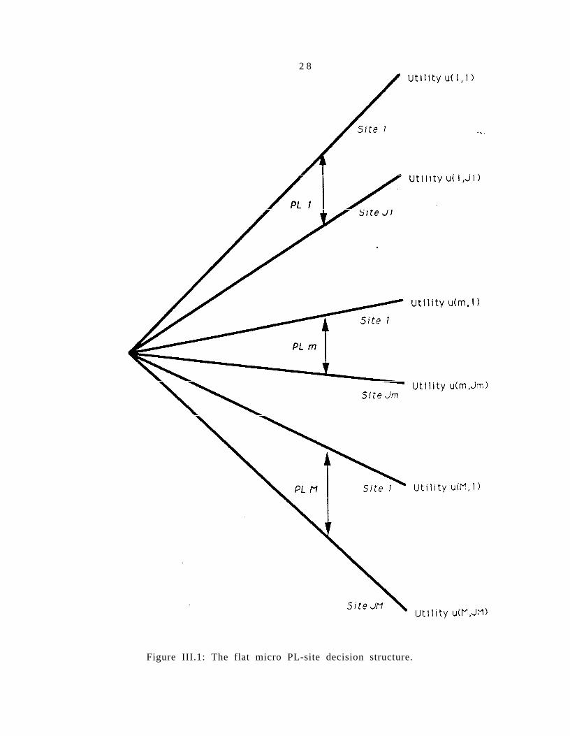
2 8

Figure III.1: The flat micro PL-site decision structure.

To avoid the IIA restriction, the nested multinomial logit (NMNL) model is better

suited for our study.

the same attributes 7 as site B, the probability ~{~,B) would probably be only half its

original level, while fi(l ,Aj will, most likely, not change. This is just an analog of the

29

famous red-bus/blue-bus problem in the transportation literature. Therefore, where

there are obvious differences in patterns of substitution and complementarity across

alternatives, the IIA assumption, and hence the MNL, is not appropriate.

Nested Multinomial Logit Model

Individuals are hypothesized to adopt a two-level tree-like deci-

sion process on any choice occasion. They first determine the target product line, and

then choose a site conditional upon the product line decision. This is illustrated in

figure III.2. The result is that the IIA property is imposed on sites within a product

line, but not across product lines.

Assume that the random

PL l arid then site j is

utility u (mj), an individual can receive from first choosing

where the attribute vector X(m,j) and random terms C,,,fi,j) are specific to the PL-site

choice (m,j), while variables in vector Z~ vary only with PLs. The PL characteristics

Z ~ are shared by all sites available to PL m. Also assume that the random terms e

follow the generalized extreme value (GEV) distribution defined below.

Definition III.2 The generalized extreme value distribution is defined as

30

Figure III.2: The two-stage micro PL-site decision structure.

31

2. G is homogeneous of degree p > 0

3. lim 2/,-a G(yl, y?: . ,yx) = ix for i = 1, 2, . . . , N

4. The sth derivative of G with respect to any combination of s distinct yr‘s,i = 1, 2, ? .‘> Ar, is non-negative if s is odd, and non-positive if 5 is even.

McFadden (1978) proves the GEV distribution implies that the probabilistic-choice

model consistent with utility maximization gives choice probability of the form

where G, is the first derivative of G with respect to y,.

Now assume that the function G is homogeneous of degree 1 and has the form

Therefore, the disturbances E have the joint distribution

(III.8)

The probability of (m, k) being chosen is then

(III.9)

(III.10)

(III.11)

where

is the inclusive value of the sites in PL m. Note that

constant (III.12)

Consequently, the IIA property continues to hold for sites in the same product line,

but not across product lines.

32

The inclusive value I, is an index of the overall quality of fishing opportunities

of the sites in PL m, or the expected maximum utility the site, of PL m can offer,

excluding the utility one can get from PL attributes 2 that do not vary across sites.

Similarly we can calculate the inclusive value

(III.13)

as an index for the desirability of participation in recreation. The value I’ represents

the expected utility of taking a fishing trip’ and will be used in the participation

decision modeling.

Estimates of the parameters can be obtained by employing a two-step procedure:

First, the estimates for ,!3; ( z 13J6) are obtained by repeatedly applying MNL to

each product line m. The inclusive values I, can then be calculated and used, along

with the PL-specific variables Z,, in the second-stage MNL estimation of Q and 6.

The original parameters ,$ can then be recovered as ,am = 6f?&. Note that in the

simple logit setup (III.7). the parameter 6 is exogenously set to 1, thus excluding the

case where different PLs have inherently different utility effects.

The way the NMNL avoids the IIA property is to allow a general pattern of depen-

dence among the choices. This is embodied by the GEV distribution assumption, as

opposed to the independent residuals assumption of the simple logit model. This can

be more intuitively seen from an alternative derivation of the NMNL by Ben-Akiva

and Lerman (1985, pp. 285-91) or Cardell and Steinberg (1988).

They start by splitting the PL-site alternative residuals into two parts and assum-

ing that

where em is the random component attributable to the product line m and common

to all sites in PL group m. This generates a correlated structure for the errors across

6 Net of the constant terms from both the site and product line levels of analysis.

33

alternatives in the same PL group W h e n ecm,k) is Weibull distributed, it can be

shown that there exist some B E [0, 1] and a random variable E,.,,: independent of

e(,,,k), such that [e,,,Se e(m,k)] is also Weibull distributed. The probability statements

derived from this specification are exactly identical to (III.9) and (III.11).

The parameter 0 is called the dissimilarity index because it indicates the share of

the common components in the error variance. The smaller 0 is, the more similar the

sites under PL m are.g Therefore, as 0 approaches 0, the nested MNL becomes more

appropriate. The flat MNL can only be justified when 8 is close to 1.

McFadden (1978) shows that a sufficient condition for a NMNL model to be

consistent with random utility maximization is that the coefficient B of the inclusive

value I lies in the [0, 1] unit interval. An estimated t9 outside the unit interval range

hence raises questions about a potential mis-specification of the model.

Estimation of the Sequential Multinomial Logit

Due to the nonlinearity and complexity of the model (III.9), estimation by max-

imum likelihood is practically infeasible. Instead, the sequential estimation method

described above is employed.

One complication arising from this stepwise procedure needs to be addressed.

Because the inclusive value index variables used in all stages above the lowest level are

in fact estimated from the lower stages, not actually observed variables, the covariance

matrices calculated by MNL will be biased and have to be corrected. lo

A more serious problem with the sequential estimation method that can not be

’ Many authors use p = 1 - f? instead of 6 as a measure to indicate the correlation amongalternatives in the same group. For example, Maddala (1983), Bockstael et al. (1986, 1988), andGreene (1989).

I” The process of correcting the estimated covariance matrix to generate consistently estimatedstandard errors is described in the Appendix in McFadden (1981). Schmalensee and Joskow (1986)also discuss techniques of using estimated parameters as independent variables.

so easily corrected is the loss of efficiency in the estimation process. Note that since

parameters 3 and 6 appear in both rklrn and ‘;;m of the probability statement (III.11),

34

the full information maximum likelihood (FIML) estimates can only be obtained by

taking derivatives of the complete log likelihood function

with respect to the parameters p, 8 and cy and setting the first derivatives to zero.

Alternatively, the multi-stage procedure estimates p’ = ,316 in the first stage by

maximizing only

and then estimates Q: and 9 in the second stage by maximizing

These estimates are thus only limited information maximum likelihood. (LIML) esti-

mates since not all available information in the data is utilized.

The Nested Mult inomial Logit Speci f icat ion

We adopt a linear utility function for this study, which implies there are no in-

come effects from quality changes. Consequently, the compensating variation and

equivalent variations for a quality change will be equsl.‘l The utility an individual i

receives from choosing PL m and site k is assumed to be

( I I I . 1 4 )

I1 Most empirical MNL studies. from the early mathematical psychology work of Luce (1959) torecent recreation demand studies of Bockstael et al. (1988) and Morey et al. (1988), adopt a linearform for the conditional utility function. Feenberg and Mills (1980) argue that, though linearity canhardly be literally true, it “may be a good approximation if the utility function is smooth and thesample variances of the parameters are not too large” (p. 112). The most important reason for ouradopting a linear utility function, however, is the ease of consumer surplus computation. When theconditional utility is nonlinear formula for the consumer surplus per choice occasion is very hard toobtain.

35

where u; is the individual constant, Em is the PL constant, .A(m,kj is the PL-site

constant, 2, is the characteristics vector that varies only with PLs, and -Xtrr.,k! are

the attributes specific to both PLs and sites. The random elements E are assumed to

follow the GEV distribution defined by (III.8).

Given the PL choice m, individual i will select a site k that offers the highest

“site” utility

The variables X we use in the estimation include site quality Q and the choice oc-

casion income net of travel costs to site k (1; - Ptk). which is available to spend on

consumption of market goods, where P,k is the travel cost of an angler i visiting site

k. Therefore, the conditional utility function Z;(,,,k) becomes

As explained above, we cannot obtain estimates for A: 77 and B at this stage; instead

we get only A’ = X,/6, 77’ = 71,!6: and /3; = /?,I6 for each PL m using the sample of

individuals who we observed choosing PL m.

In our analysis (as is generally the case) we do not have data on choice occasion

income. These missing data are not a problem in the site-choice level of analysis,

because the income is constant across sites and so drops out in the estimation (which

employs differences between the conditional utility functions.) However, when the

marginal utility of income is not constant across alternatives in a nested MNL model,

the lack of choice occasion income will affect the higher-level estimation - in our

analysis, the choice of product line - and the welfare calculations.

Consequently, we derive in some detail below the value of the lower-level inclusive

value index for sites in product line rn: I,,,, and of the higher-level inclusive value

index across product lines. The goal is to explicitly identify the role of the choice

occasion income variable. All inclusive value calculations are performed separately

36

for each trip duration category.

The inclusive value I, for sites in product line m, as defined in (III.12), is

The estimated parameter 7 of the travel cost variable P,, is individual i’s constant

marginal utility of income for product line m. Because of missing data on choice

occasion income 1’-%: we can only calculate the pseudo-inclusive value 7, from the

estimates X’: q:, and pk.

In the upper-level PL-choice modeling in the NMNL we estimate the parameters

of the PL conditional indirect utility function

where I, is the inclusive value index calculated above from the lower-level site-choice

MNL estimation. As defined by (III.13), the inclusive value of taking a trip is

37

If 77, = 7 for all m, then we can further simplify the formula:

(III.15)

The individual-specific constants ~i are not identifiable, and as stated above, we do

not know the choice occasion income T-,. Therefore, we cannot calculate the real level

I:, and so will use the pseudo-inclusive value I; in chapter V for the calculation of

consumer surplus.

Because Q; - 77)‘; is constant across product lines (assuming 77, = 7): estimation

with 7: is equivalent to estimation with 1;. In Chapter V, we further show that if

the marginal utility of income is constant across alternatives, the lack of choice oc-

casion income does not pose problems for the welfare analysis. However, if MU is

not constant across product lines, then we cannot calculate 1; as the three separable

components in (III.15): the choice occasion income term remains an integral compo-

nent of the calculation. As a consequence, estimation using 7: in place of 1; yields a

mis-specification.

In our NMNL estimation procedure below, we do not impose the constraint of con-

stant MUI across product lines within a duration group,12 due to the computational

I2 We would not expect constant MUI across duration groups, but this issue does not pose anydifficulties because we model trip-duration choice within the participation model.

38

complexity it would cause, though such a restriction seems conceptually appropriate.

We have developed a procedure for handling the problems posed by not constraining

the MUI to be constant. In the process of specifying the correct consumer surplus

formulas for the case of varying marginal utility of income, we derive in Chapter

V a “weighted” marginal utility of income, where the weights represent the ex-post

probabilities of choosing the alternative. The weighted MUI serves the same role in

the consumer surplus formula that the (constant) MUI serves in the simpler context.

We will substitute the weighted MUI in the calculation of If, in lieu of performing

the NMNL estimation with cross-estimation constraints. Employing this conceptual

framework, use of c in the estimation procedure is not a mis-specification.

The Valuat ion of Time

The Analysis Framework

A critical component of the conditional indirect utility function for site alternatives

specified above in equation III.14 is the travel cost Plk per trip by individual i to site

I:. Conceptually. travel cost consists of two components - distance costs and time

costs. As discussed above in Chapter II the time cost component is controversial.

We derive in some detail several models which support several different treatments of

the opportunity costs of trip time in the discrete choice literature. We show how the

models imply not only different measures of travel cost but also different definitions

of the choice set of feasible sites.

Anglers are assumed to maximize utility subject to a full-income constraint for

the choice occasion, where full income refers to the money budget plus the value of

time, following the household production function literature. Note that, among the

sites within the angler’s choice set, we only observe the amount of time the individual

39

allocated for a trip to the chosen site. We must make assumptions about how much

time an individual would allocate for trips to other sites.

The first two frameworks are based on an assumption that total trip time will

be the same for all sites (as for the chosen site); we label this the “exogenous total

trip time” framework. The two variants we develop employ alternative measures of

trip time. The third framework is based on the assumption that on-site time will be

the same for all sites (as for the chosen site); we label this the “exogenous on-site-

time” framework. We show below in the Appendix the potentially large effect these

differences may have on model results.

Variable Definitions

We first define the following variables for our discussion.

S = market goods (set price=1 as numeriare

D = number of days in trip

zc: = post-tax wage rate

c = vehicle operating cost per mile

s = driving speed (miles per hour)

qs = quality of site j, where j = 1, . . , J

D3 = round-trip distance in miles to site j

P, = c Dj = round trip travel cost to site j

R, = D,/s = round trip travel time in hours to site j

S, = time spent on site j in hours

T, = R,-G,= total trip time to site j in hours

C = choice occasion time in hours

y = money allocated to the recreational choice occasion

I7 = full income allocated to the choice occasion

4 0

Exogenous Trip Time

Within the exogenous trip-time framework, we impose the assumption that an in-

dividual allocates all of the choice occasion time C either to visiting a site j, thereby

incurring round-trip travel time R, plus on- site time Sj, or to other activities (work-

ing, other recreation). We can write the generalized time budget, conditional upon

participation, for the choice occasion:

As defined previously, the indicator E, = 1 if site j is chosen for the visit, and E, = 0,

otherwise. If Ek = 1, then 6, = 0 for all j # k.

The sources of full income 1’ include WC, time during the choice occasion valued

at the post-tax wage rate u’:13 and y, the money income allocated for expenditure

during the period:

(III.16)

The uses of full income during the period are expenditures during the trip on market

I’ Recognizing that recreational activities take up time, much of the recreation demand literaturerelates the opportunity time costs to the wage income forgone when a trip is taken. However, thelabor supply literature now recognizes that work, time may not be a continuous choice variable overwhich individuals can freely trade-off income and recreation at the wage rate. Only individuals withflexible work hours can adjust their marginal rate of substitution between work and recreation andmake it equal to their marginal wage rates. These individuals are said to be at interior solutions.Others, who either have to work fixed hours or do not work at all, are at corner solutions, and theirwage rates cannot serve as the value of their leisure time.

Some authors in the recreation demand literature have also adopted this view and have treatedinterior solutions and corner solutions differently. For people at interior solutions, work time is attheir discretion, and trip time can be traded for income at their marginal wage rate. For otherswithout such freedom, no opportunity, wage cost exists since they cannot increase their work efforteven if no trip is taken.

Unfortunately no wage rate was directly measured in our data, so the above treatment is im-possible. The budget frontier therefore has to be assumed a straight line, and people are assumedto be at interior solutions. We assume that people value their time at their wage rate, calculated asannual personal income divided by projected working hours per year.

41

goods X plus distance costs and time costs to the chosen site:

Setting sources equal to uses, we have

(III.17)

Conditional upon participation in recreation at site j (i.e., Sj = 1), we can solve for

A’ = y - P,. The indirect utility function conditional upon participation at site j is

Assuming a linear functional form, the conditional indirect utility function becomes

The important point to note is that time costs have completely dropped out of the

travel cost measure for site choice, because the amount of time allocated to "pro-

ducing" recreation (the choice occasion) equals the trip duration. The use of the

standard travel cost variable incorporating both time and distance costs cannot be

supported in this framework. I4 With a conditional direct utility function of the form

l4 Besides monetary vehicle costs P,. the amount of driving could conceivably have at least twoother effects on an angler’s utility: a reduction in available fishing time S, and the (dis)utility ofdriving h!, itself. A more elaborate and complete utility function will, therefore, be

The linear estimating function is then

42

I*j(s, q,), the time costs affect angler decision-making only at the higher level where

the participation choices for each trip duration are made.

We suggest two alternative methods for implementing the exogenous trip duration

model: the first measures trip duration in hours, based on the self-reported hours (and

days) for the beginning and end of the trip; the second measures trip duration based

on the number of days the individual reported being away. Though the conditional

indirect utility specification is the same, the definition of the choice set for each

individual, the consistency checks for selecting individuals into the sample, and the

value of the time cost variable in the participation model differ.

Hypothesis 1: Exogenous Trip Time (Using Self-Reported Trip Hours)

In this case, total trip time T is based on self-reported trip duration. The amount

of income allocated to the choice occasion is calculated as (III.16). but has no practical

significance in the site choice analysis.

Let constant h be the presumed number of hours people are awake and active

during a day. Its complement h’ (E 24 -h) is then the time in hours people rest each

day. For a trip of D days, people necessarily must rest for (D - 1) nights, a total of

(D - 1) h’ hours, at their fishing site or on the road. Therefore. we impose two time

constraints for a D-day trip to any potential site j :

A 1 : T,<_h’dIhy(D-!)h’

A2 : S, = T , -R, 2 (D - l)h’

The real marginal utility of income 7 = O1 cannot be identified. The marginal utility of incomemeasure we obtain without including the R, and S, terms in 1; is q’ = /?I - e, which is actuallya combination of the various driving effects. Anticipating negative utility from driving and reducedfishing time, we have 02 < 0 and ,B, > 0. Therefore,

The resulting consumer surplus we derive using 7’ will consequently be an under-estimate of its realvalue.

43

Constraint A1 asserts that the total trip duration cannot exceed the limit of h’ hours,

which is the sum of active and resting time during the day. Constraint A2 enforces

that people still have time left after accounting for driving and resting to fish and

enjoy site amenities. Combined: they imply that R, 5 D h. In words; this posits that

round-trip driving time (R,) cannot take up all the time people are awake during the

trip.

Any site j that violates either A1 or A2 is considered infeasible for a visit on

the choice occasion in question. The time constraints A1 and A2 thus define the

individual choice set of feasible sites. People whose reported destination sites of the

observed trips violate these time constraints are thus treated as outliers and deleted

from the MNL sample. l5 The value selected for h hence plays a critical role in the

site choice analysis. i6 When a larger h is used: more people will be included in the

sample, and more sites will be included in each individual’s choice set.

To be included in the MNL sample: each angler’s destination site k must satisfy

time constraints A1 and A2 specified above. That is,

Tk 5 h-s1 :

I&=Tk-Rk >(D-1)h’-

For an individual in the sample S, who chooses site k (and hence has a pre-determined

total trip duration Tk). site j will be included in his or her choice set if and only if

T, E Tk 5 h-Cl :

Sj=Tk-Rj 2(D-l)h’

r5 In the actual implementation of the model, an individual can be excluded from entering theMNL sample due to three reasons: (1) the trip duration data T is missing, (2) the observed chosensite itself violates the time constraint A1 and/or A2, or (3) the chosen site is the only feasible site,so no other site is contained in his or her choice set. People who are left out from the site MNLestimation for the third reason may be included in the upper level PL MNL estimation because theinclusive value can still be calculated even though there is only one feasible site for the chosen PL.

iG The choice set definition in turn has direct effects on the MNL and total trip estimation, as wellas the final welfare calculation.

44

The satisfaction of the first constraint of Ci is guaranteed since it is exactly the same

as the first restriction of Si for inclusion in the sample. The restrictions of Si are

applied to the selected sites, while the restrictions of are applied to all other sites.

Hypothesis 2: Exogenous Trip Time (Using Total Trip-Days)

In this case, we eschew using self-reported measures of total trip time and alter-

natively impose the assumption that the total trip duration T equals the maximum

number of trip hours allowed in a D-day trip, h -. Therefore, T = h‘ = Dh -(D -1) h’ .

This procedure eliminates the measurement error and missing data problems posed

by the first procedure: but incorporates probably greater measurement error in the

trip time (cost) variable by imposing the assumption that each trip uses all waking

hours of the day.17

Under this hypothesis, the conditions A1 and A2 combined are equivalent to

S2: R&Dh.

The choice set of an individual can also be computed by including in it any site j

that satisfies

Cz: R,<Dh.

Hypothesis 3: Exogenous On-Site Time

The final hypothesis imposes an alternative assumption that on-site time is fixed

across site choices: rather than trip duration. To ensure an exogenously defined choice

occasion, we must include in the model the possibility of ‘slack time’ during the choice

occasion Even using this device. there is some question for day trips as to whether

I7 We can calculate the difference from the site-hours variable, but we do not know how muchmeasurement error there is in site-hours.

4 5

one of the conditions for welfare analysis necessarily holds: that only one trip could

be taken during the choice occasion I6 We rewrite the time-budget from above to

acknowledge that choice occasion time C and trip time T are no longer assumed to

be the same duration:

where 6, is slack, and C = h’ = D h - (D - 1) h ’ .

The solution to equation (III.17) in which we set sources equal to uses is:

By assumption, y, C, and S, are constant across sites, and so are not relevant to the

site choice decision-making. The measure of travel cost, however, is (-P, - w&j):

the time cost of travel is included along with the distance cost! unlike for the models

above. in which only the distance cost ( -PJ) is included.

The conditions an individual must meet to get into sample Ss are the same con-

straints A1 and A2 that define S, above. Therefore , 5s = S,. For an individual

i in the sample Ss whose actual destination is site k, the constant on-site time is

calculated to be

The choice set C’s of i is defined by including any site j that satisfies

Now the second constraint of C’s is always satisfied.

Though the two samples of anglers S, and Ss, defined respectively for the exoge-

nous trip duration and the exogenous on-site time hypotheses, are identical, there is

I6 This hypothesis is adopted by McConnell et al. (1990) and Parsons and Kealy (1990). The latterassumes that all anglers spend a fixed amount of four hours on site.

46

no relationship between the choice sets Ci and Ca defined for an individual under the

alternative hypotheses. ig

It is also obvious that

since for S2 (1) the deletions necessitated by S, and S3 due to to missing data on

self-reported trip-lengths are avoided, and (2) the trip durations in S2 are assumed to

be their maximum value h’. It can further be shown that, for people in both samples

Si and Sz,

and, for people in both samples Ss and S2,

We will show the sensitivity of the model to the different trip time hypotheses in

the Appendix.

‘a It is easy to show this with examples. Suppose h = 15 and D = 1. For an angler with Tb = 5and Rk = 2, a site j with R, = 6 will be in set CJ, whereas not in Cr. But if Tk = 14. Rk = 1and R, = 4, constraints for Ca will be violated, while those for Ct are satisfied. The first exampleis a short day trip (e.g., an afternoon trip) to a nearby site. In this case faraway sites might beincluded in C3 and excluded from Cr. The second example is a long day trip (e.g.. a whole-dayfishing excursion) to a nearby site. In this case farther sites will probably be left out from CJ; butstill incorporated in Ct. Conceivably this will mainly happen to people taking day trips, as mostsites will be available to all anglers taking long trips.