Embed Size (px)
Citation preview
Naval Research LaboratoryStennis Space Center, MS 39529-5004
NRL/MR/7320--15-9574
Approved for public release; distribution is unlimited.
Validation Test Report for the Navy CoastalOcean Model Four-Dimensional VariationalAssimilation (NCOM 4DVAR) SystemVersion 1.0Scott Smith matthew carrier hanS ngodock Jay Shriver PhiliP muScarella
Ocean Dynamics and Prediction Branch Oceanography Division
heather Penta Suzanne carroll
Vencore Services and Solutions Group Stennis Space Center, Mississippi
September 14, 2015

i
REPORT DOCUMENTATION PAGE Form ApprovedOMB No. 0704-0188
3. DATES COVERED (From - To)
Standard Form 298 (Rev. 8-98)Prescribed by ANSI Std. Z39.18
Public reporting burden for this collection of information is estimated to average 1 hour per response, including the time for reviewing instructions, searching existing data sources, gathering and maintaining the data needed, and completing and reviewing this collection of information. Send comments regarding this burden estimate or any other aspect of this collection of information, including suggestions for reducing this burden to Department of Defense, Washington Headquarters Services, Directorate for Information Operations and Reports (0704-0188), 1215 Jefferson Davis Highway, Suite 1204, Arlington, VA 22202-4302. Respondents should be aware that notwithstanding any other provision of law, no person shall be subject to any penalty for failing to comply with a collection of information if it does not display a currently valid OMB control number. PLEASE DO NOT RETURN YOUR FORM TO THE ABOVE ADDRESS.
5a. CONTRACT NUMBER
5b. GRANT NUMBER
5c. PROGRAM ELEMENT NUMBER
5d. PROJECT NUMBER
5e. TASK NUMBER
5f. WORK UNIT NUMBER
2. REPORT TYPE1. REPORT DATE (DD-MM-YYYY)
4. TITLE AND SUBTITLE
6. AUTHOR(S)
8. PERFORMING ORGANIZATION REPORT NUMBER
7. PERFORMING ORGANIZATION NAME(S) AND ADDRESS(ES)
10. SPONSOR / MONITOR’S ACRONYM(S)9. SPONSORING / MONITORING AGENCY NAME(S) AND ADDRESS(ES)
11. SPONSOR / MONITOR’S REPORT NUMBER(S)
12. DISTRIBUTION / AVAILABILITY STATEMENT
13. SUPPLEMENTARY NOTES
14. ABSTRACT
15. SUBJECT TERMS
16. SECURITY CLASSIFICATION OF:
a. REPORT
19a. NAME OF RESPONSIBLE PERSON
19b. TELEPHONE NUMBER (include areacode)
b. ABSTRACT c. THIS PAGE
18. NUMBEROF PAGES
17. LIMITATIONOF ABSTRACT
Validation Test Report for the Navy Coastal Ocean Model Four-Dimensional Variational Assimilation (NCOM 4DVAR) SystemVersion 1.0
Scott Smith, Matthew Carrier, Hans Ngodock, Jay Shriver, Philip Muscarella,Heather Penta,* and Suzanne Carroll*
Naval Research LaboratoryOceanography DivisionStennis Space Center, MS 39529-5004 NRL/MR/7320--15-9574
Approved for public release; distribution is unlimited.
*Vencore, Services and Solutions Group, Stennis Space Center, MS
UnclassifiedUnlimited
UnclassifiedUnlimited
UnclassifiedUnlimited
UnclassifiedUnlimited
115Scott Smith
(228) 688-4630
4DVARData assimilation
Ocean analysisValidation
Ocean prediction
This report provides the results of a series of validation experiments that compare the prediction accuracy and efficiency of the Navy Coastal Ocean Model Four-Dimensional Variational Assimilation (NCOM 4DVAR), version 1.0, relative to the current, operational version of the Relocatable (Relo) NCOM. The NCOM 4DVAR uses the more advanced representer-based 4DVAR method to compute analyses. The validation experiments include the application of NCOM 4DVAR in nine regional domains. Three of these experiments were performed in the Okinawa Trough, the U.S. East Coast, and the Northern Arabian Sea in an operational mode on the Operational Oceanography Center (OOC). Overall, the validation results reveal that the applications of NCOM 4DVAR have improved performance in terms of reduced average Root Mean Squared (RMS) errors for temperature and salinity analyses and forecasts when compared to similar applications of the operational Relo NCOM system.
14-09-2015 Memorandum Report
Office of Naval ResearchOne Liberty Center875 North Randolph Street, Suite 1425Arlington, VA 22203-1995
73-4727-24-5
ONR
0602435N

ii
iii
TABLEOFCONTENTSFIGURES AND TABLES ......................................................................................................................................... v
1.0 INTRODUCTION ..................................................................................................................................... 1
1.1 NAVY COASTAL OCEAN MODEL (NCOM) ..................................................................................................................... 1 1.2 NAVY COUPLED OCEAN DATA ASSIMILATION 3D VARIATIONAL ANALYSIS (NCODA‐VAR) SYSTEM, VERSION 3.43 .................... 2 1.3 RELOCATABLE NCOM (RELO NCOM) .......................................................................................................................... 3 1.4 NAVY COASTAL OCEAN MODEL FOUR DIMENSIONAL VARIATIONAL SYSTEM (NCOM 4DVAR) VERSION 1.0 ............................. 3 1.5 DOCUMENT OVERVIEW .............................................................................................................................................. 6
2.0 VALIDATION METRICS............................................................................................................................ 9
2.1 ANALYSIS / FORECAST METRICS ................................................................................................................................... 9 2.2 ENGINEERING METRICS .............................................................................................................................................. 9 2.3 SUBVERSION REPOSITORY ........................................................................................................................................... 9
3.0 VALIDATION TEST DESCRIPTION AND RESULTS: OKINAWA TROUGH ................................................. 11
3.1 TEST AREA AND OBSERVATIONS: OKINAWA TROUGH ..................................................................................................... 11 3.2 MODEL SETUP: OKINAWA TROUGH ............................................................................................................................ 12
3.2.1 Experiment Overview ............................................................................................................................. 12 3.2.2 Domain Details ....................................................................................................................................... 13 3.2.3 Experiment Objectives ............................................................................................................................ 13
3.3 RESULTS: OKINAWA TROUGH .................................................................................................................................... 14 3.3.1 Time Distribution of Errors ..................................................................................................................... 17 3.3.2 Profile Distribution Errors ....................................................................................................................... 27 3.3.3 NAVOCEANO Glider and Aerial XBT (AXBT) Comparisons ...................................................................... 32 3.3.4 Surface Duct Predictions ......................................................................................................................... 34
3.3.4.1 Sonic Layer Depth Studies ................................................................................................................................... 34 3.3.4.2 Predictions of Surface Layer Trapping of Acoustic Frequencies .......................................................................... 36 3.3.4.3 Sonic Layer Depth Distributions ......................................................................................................................... 38
4.0 RESULTS: OTHER REGIONS .................................................................................................................. 43
4.1 MONTEREY BAY ...................................................................................................................................................... 43 4.1.1 Model Set‐up: Monterey Bay .................................................................................................................. 44 4.1.2 Results: Monterey Bay ............................................................................................................................ 44
4.2 GULF OF MEXICO .................................................................................................................................................... 48 4.2.1 Model Set‐up: Gulf of Mexico ................................................................................................................. 49 4.2.2 Results: Gulf of Mexico ........................................................................................................................... 50
4.2.2.1 Velocity Assimilation .......................................................................................................................................... 55 4.2.2.2 SSH Assimilation ................................................................................................................................................. 57
4.3 OTHER LOCATIONS USING NCOM 4DVAR ................................................................................................................. 59 4.3.1 Pacific Rim (RimPac) Hawaii ................................................................................................................... 60 4.3.2 Middle Atlantic Bight .............................................................................................................................. 62 4.3.3 Southern California ................................................................................................................................. 64 4.3.4 Kuroshio Extension ................................................................................................................................. 65
5.0 OPERATIONAL IMPLEMENTATION OF NCOM 4DVAR ......................................................................... 69
5.1 RESOURCE REQUIREMENTS ....................................................................................................................................... 69 5.2 REAL TIME DEMONSTRATION ON THE OOC .................................................................................................................. 73
5.2.1 Okinawa Trough ..................................................................................................................................... 74 5.2.2 North Arabian Sea .................................................................................................................................. 75 5.2.3 U.S. East Coast ........................................................................................................................................ 79
6.0 CONCLUSIONS ..................................................................................................................................... 83
7.0 FUTURE WORK ..................................................................................................................................... 85

iv
8.0 ACKNOWLEDGEMENTS........................................................................................................................ 87
9.0 REFERENCES......................................................................................................................................... 89
9.1 CITED REFERENCES .................................................................................................................................................. 89 9.2 GENERAL REFERENCES ............................................................................................................................................. 93
10.0 ACRONYMS AND ABBREVIATIONS ....................................................................................................... 97
11.0 APPENDIX: MODEL SET‐UP AND NAMELIST ......................................................................................101

v
FIGURESANDTABLES
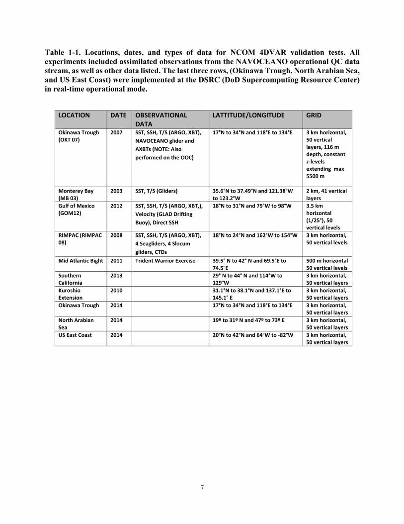
Table 1‐1. Locations, dates, and types of data for NCOM 4DVAR validation tests. All experiments included
assimilated observations from the NAVOCEANO operational QC data stream, as well as other data
listed. The last three rows, (Okinawa Trough, North Arabian Sea, and US East Coast) were
implemented at the DSRC (DoD Supercomputing Resource Center) in real‐time operational mode. ... 7
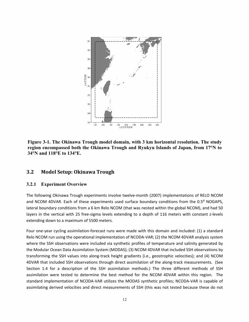
Figure 3‐1. The Okinawa Trough model domain, with 3 km horizontal resolution. The study region
encompassed both the Okinawa Trough and Ryukyu Islands of Japan, from 17°N to 34°N and 118°E to
134°E. .................................................................................................................................................... 12
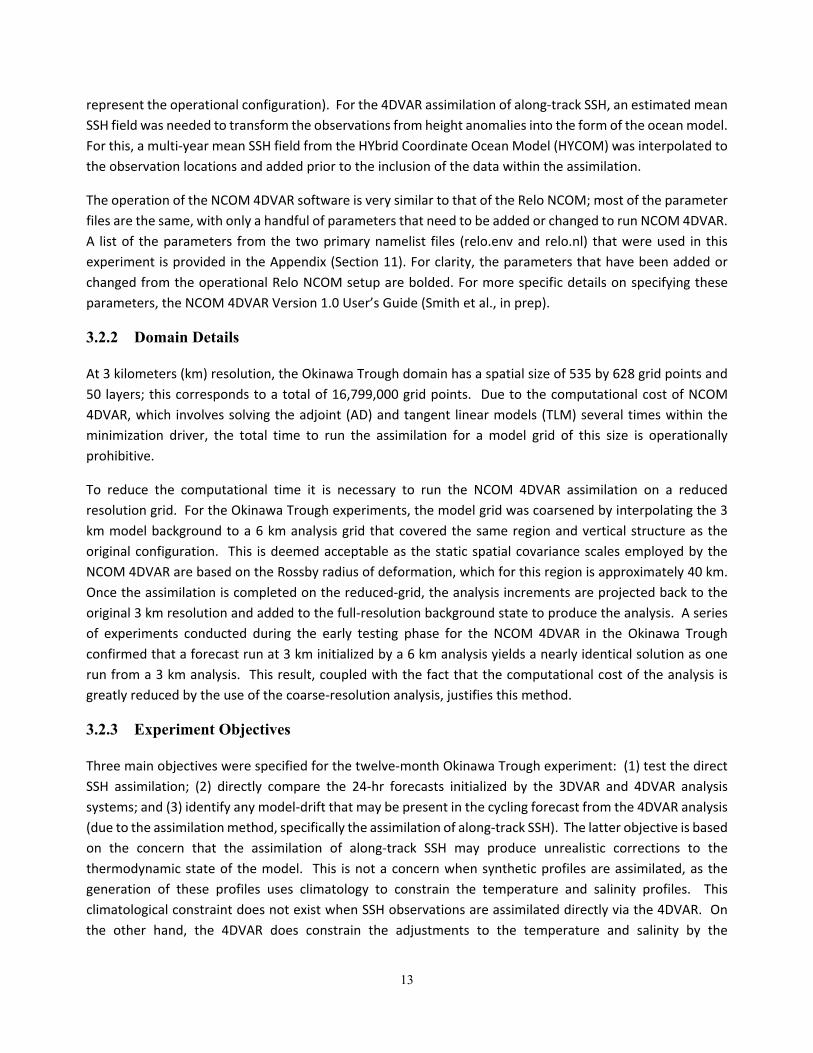
Figure 3‐2. Global Fit (space and time) of the 24‐hr forecast (black) and the analysis (white) of the 4DVAR SYN
to the assimilated observations of temperature (left) and salinity (right) for the 12‐month Okinawa
Trough run, as a function of the number of standard deviations of the prescribed observation error.
There is no boxplot for SSH, since direct SSH observations were not assimilated. .............................. 14
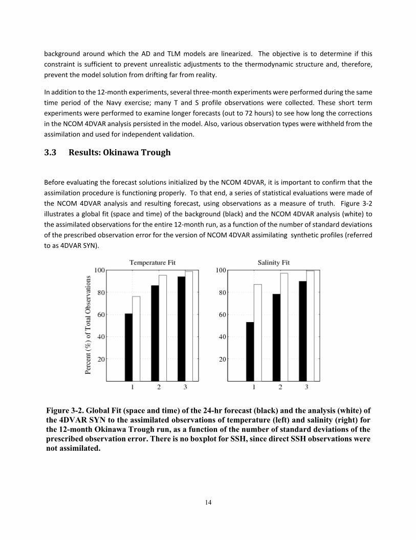
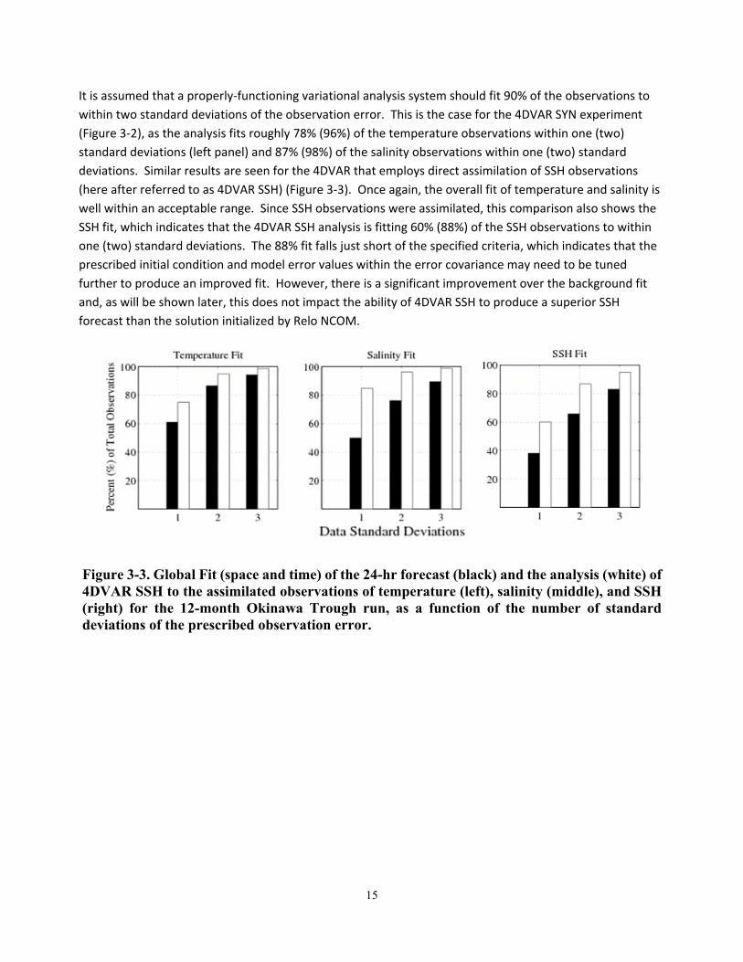
Figure 3‐3. Global Fit (space and time) of the 24‐hr forecast (black) and the analysis (white) of 4DVAR SSH to
the assimilated observations of temperature (left), salinity (middle), and SSH (right) for the 12‐month
Okinawa Trough run, as a function of the number of standard deviations of the prescribed observation
error. ..................................................................................................................................................... 15
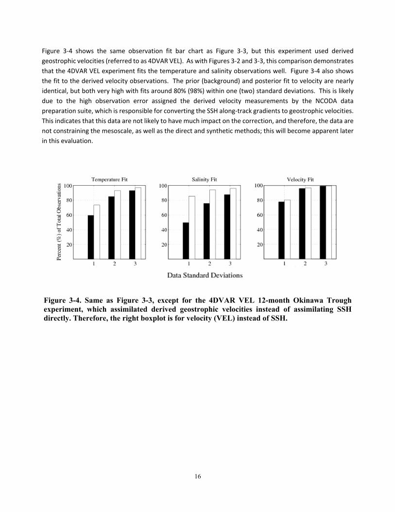
Figure 3‐4. Same as Figure 3‐3, except for the 4DVAR VEL 12‐month Okinawa Trough experiment, which
assimilated derived geostrophic velocities instead of assimilating SSH directly. Therefore, the right
boxplot is for velocity (VEL) instead of SSH. .......................................................................................... 16
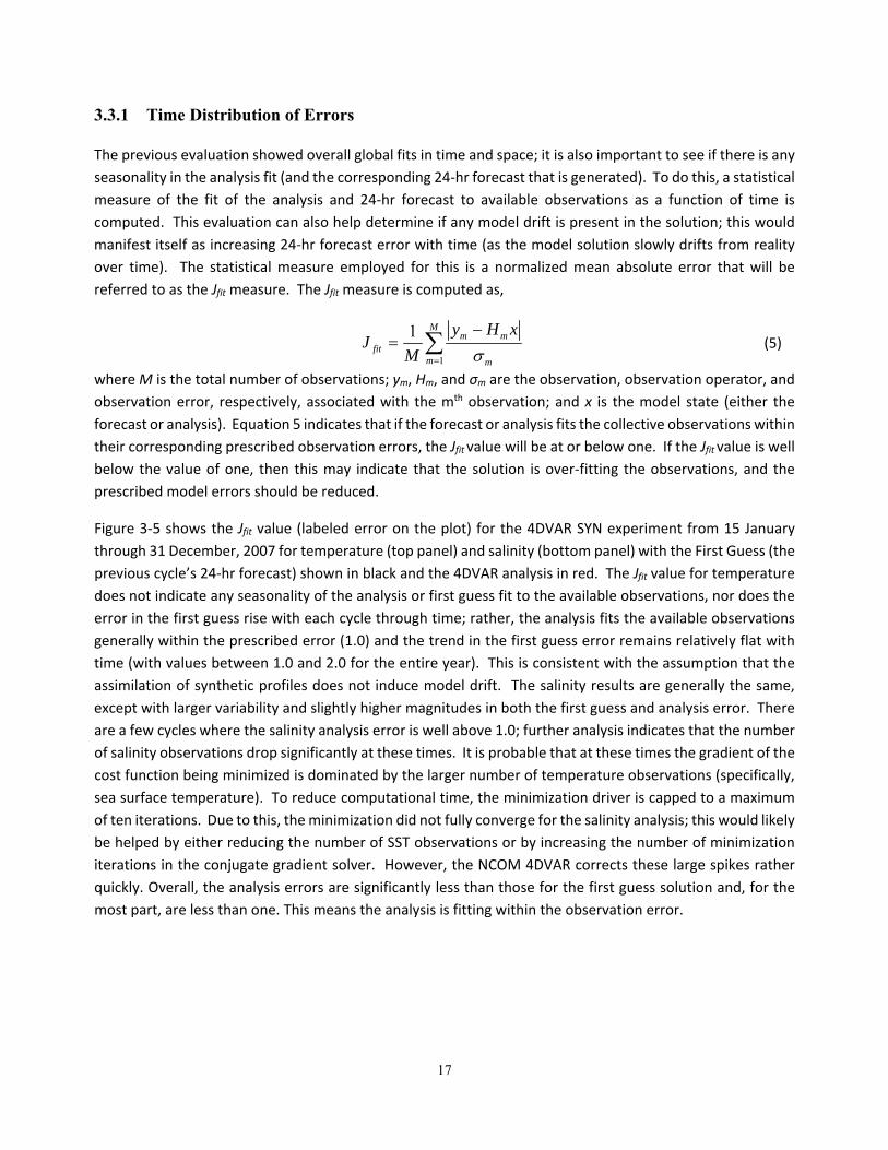
Figure 3‐5. Errors in temperature (top) and salinity (bottom) solutions from the first guess (black) and the
analysis (red) relative to the observations that were assimilated for the 4DVAR SYN experiment. Since
SSH observations were not assimilated directly, there is no error plot for SSH. These errors span the
entire year of the Okinawa Trough experiment (15 January through 31 December 2007) and are
normalized by the corresponding observation error (Jfit, see Equation 5). .......................................... 18
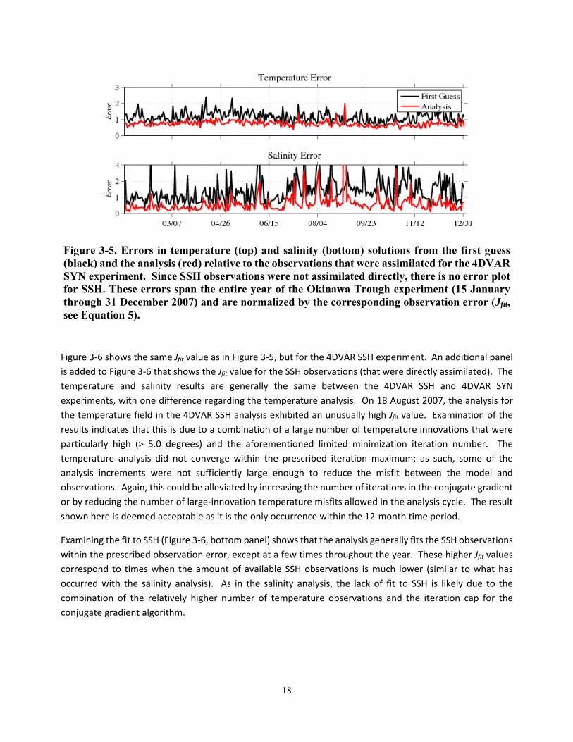
Figure 3‐6. Errors in temperature (top), salinity (middle), and SSH (bottom) solutions from the first guess
(black) and the analysis (red) relative to the observations that were assimilated for the 4DVAR SSH
experiment, which assimilated SSH directly. These errors span the entire year of the Okinawa Trough
experiment (15 January through 31 December 2007) and are normalized by the corresponding
observation error (Equation 5). ............................................................................................................ 19
Figure 3‐7. Same as Figure 3‐6, except for the 4DVAR VEL 12‐month Okinawa Trough experiment, which
assimilated derived geostrophic velocities instead of assimilating SSH directly. Therefore, the bottom
plot is for velocity (VEL) instead of SSH. ............................................................................................... 20
Figure 3‐8. Comparison of the 24‐hr SSH forecast error from the year‐long Relo NCOM (black) and the 4DVAR
SYN (red) experiments, as compared to available ALPS SSH observations throughout the Okinawa
Trough domain. Equation 5 is used to compute the normalized error. .............................................. 21
Figure 3‐9. Similar to Figure 3‐8, except this is for the 4DVAR SSH experiment. ............................................. 22
Figure 3‐10. Similar to Figure 3‐8, except this is for the 4DVAR VEL experiment. ........................................... 22
Figure 3‐11. Absolute value of difference between the temperature profile observations and the background
(top) and analysis (bottom) solutions for the year‐long Okinawa Trough 4DVAR SYN experiment. The
vi
white gaps are the result of no temperature observations at those particular depths and times. The
depth range was cut off at 250 m because there are few observations below this depth. ................. 23
Figure 3‐12. Similar to Figure 3‐11, except these are for salinity. .................................................................... 24
Figure 3‐13. Difference between the temperature profile observations and the background (top) and analysis
(bottom) solutions for the 4DVAR SSH experiment that assimilated SSH observations directly. ........ 25
Figure 3‐14. Similar to Figure 3‐13, except these are for salinity. ................................................................... 25
Figure 3‐15. Difference between the temperature profile observations and the background (top) and analysis
(bottom) solutions for the 4DVAR VEL experiment. ............................................................................. 26
Figure 3‐16. Similar to Figure 3‐15, except for salinity. ................................................................................... 26
Figure 3‐17. Comparison of 24‐hr forecast RMS profile errors between the 4DVAR SYN (red), 4DVAR SSH
(blue), 4DVAR VEL (green), and Relo NCOM (black) experiments for temperature profiles (left panel)
and salinity profiles (right panel). These are from the year‐long experiments in the Okinawa Trough.
The value N is the total number of profile observations used in these statistics. ................................ 28
Figure 3‐18. Comparison of 24‐hr forecast RMS profile errors between the 4DVAR SYN (red) and Relo NCOM
(black) experiments for temperature profiles (left panel) and salinity profiles (right panel). These are
from the 3‐month experiments (August – October) in the Okinawa Trough. The value N is the total
number of profile observations used in these statistics. ...................................................................... 30
Figure 3‐19. Same as Figure 3‐18, except this is for the 4DVAR SSH experiment. .......................................... 31
Figure 3‐20. Comparison of 24‐hr (Solid) and 96‐hr (dashed) forecast RMS profile errors between the 4DVAR
SYN (red), 4DVAR SSH (blue), and Relo NCOM (black) experiments for temperature profiles (left panel)
and salinity profiles (right panel). These are from the 3‐month experiments (August – October) in the
Okinawa Trough. The value N is the total number of profile observations used in these statistics. .. 32
Figure 3‐21. The layer‐by‐layer Jfit error values for the 4DVAR SSH 24‐hr forecast (red) versus the Relo NCOM
experiment 24‐hr forecast (black) for temperature (left panel) and salinity (middle panel) computed
against withheld glider observations (right panel). .............................................................................. 33
Figure 3‐22. The layer‐by‐layer Jfit error values for the 4DVAR SSH 24‐hr forecast (red) versus the Relo NCOM
24‐hr forecast (black) for temperature (left panel) and salinity (middle panel) computed against
withheld AXBT data (right panel). There are no salinity AXBT data, therefore the middle panel is all
zero. ....................................................................................................................................................... 34
Table 3‐1. Sonic Layer Depth (SLD) prediction errors of the Relo NCOM and NCOM 4DVAR analysis, along with
their ensuing 24‐hr, 48‐hr, 72‐hr, and 96‐hr forecasts. Errors are relative to the SLD computed from
all NAVOCEANO restricted observations. The experiments with the best correlation are highlighted in
yellow. ................................................................................................................................................... 35
Figure 3‐23. Predictability of surface layer trapping at acoustic frequencies (Hz) ranging from 50 ‐ 3500 Hz
using the analysis fields from the 3‐month Okinawa Trough Relo NCOM (left), the 4DVAR SSH (middle),
and the 4DVAR SYN (right) experiments. The values in parentheses in the legends denote the average
over all frequencies of each corresponding curve. ............................................................................... 37
Figure 3‐24. Same as Figure 3‐23, except that this is for the 24‐hr forecast. .................................................. 37
Figure 3‐25. Same as Figure 3‐23, except that this is for the 48‐hr forecast. .................................................. 37
Figure 3‐26. Same as Figure 3‐23, except that this is for the 72‐hr forecast. .................................................. 38
Figure 3‐27. Same as Figure 3‐23, except that this is for the 96‐hr forecast. .................................................. 38
vii
Figure 3‐28. Okinawa Trough 2D histograms of SLD (m) of Relo NCOM (left), 4DVAR SSH (middle), and 4DVAR
SYN (right) analyses relative to all NAVOCEANO restricted profile observations during the 3‐month
time period of 1 August to 31October 2007. The diagonal black line denotes the locations on each
histogram where the modelled SLD matches the observed and the color bar denotes the number of
counts and is on a log scale. .................................................................................................................. 39
Figure 3‐29. Same as Figure 28, except this is for the 24‐hr forecast. ............................................................. 40
Figure 3‐30. Same as Figure 28, except this is for the 48‐hr forecast. ............................................................. 40
Figure 3‐31. Same as Figure 28, except this is for the 72‐hr forecast. ............................................................. 41
Figure 3‐32. Same as Figure 28, except this is for the 96‐hr forecast. ............................................................. 41
Figure 3‐33. 2D histograms showing the difference in SLD counts between the Relo NCOM and 4DVAR SYN
analyses (left) and 96‐hr forecasts (right). Blue (red) squares signify that 4DVAR SYN has more (less)
SLD combination counts than Relo NCOM............................................................................................ 42
Figure 4‐1. The Monterey Bay model domain with bathymetry contours and the profile locations, including
the numbered profiles (in red) where the assimilated solution was evaluated. The domain covers 35.6°
N to 37.49° N and 121.38° W to 123.2° W. The model was initialized 1 August 2003 and ran for one
month until 1 September 2003. ............................................................................................................ 44
Figure 4‐2. Time evolution of the absolute value of the innovation (top) and the analysis error (bottom) at
profile location 3 (Figure 4‐1), for temperature (left) and salinity (right) in Monterey Bay, 2003. ...... 45
Figure 4‐3. Absolute model temperature (left) and salinity (right) discrepancies to non‐assimilated glider
observations for the free run (top), first guess (middle), and analysis (bottom) in Monterey Bay, 2003.
............................................................................................................................................................... 46
Figure 4‐4. Cumulative bar chart showing the percentage of the number of observations that are matched by
the free running model (black), the first guess (grey), and the analysis (white) as a function of the
number of observation standard deviations. The MODAS experiment is shown on the left and AOSN II
experiment on the right. ....................................................................................................................... 47
Figure 4‐5. (Left) The model domain for the Gulf of Mexico experiment extends from 18⁰ N to 31⁰ N and 79⁰ W to 98⁰ W with a 4 km resolution. (Right) Location of each GLAD drifter velocity observation from
1 August to 30 September 2012 (observations plotted at daily intervals) (Carrier et al., 2014). ......... 48
Figure 4‐6. Jfit metric values (Equation 5) for the NCOM free‐run (FR) model solution (solid line) and the
4DVAR analysis solution assimilating only T and S (dash line) measured against assimilated
temperature observations (top panel), salinity observations (middle panel), and unassimilated GLAD
velocity observations (bottom panel). Valid from 1 August through 30 September 2012 in the GOM.
............................................................................................................................................................... 50
Figure 4‐7. Jfit metric values for the analysis solution assimilating just temperature and salinity (solid line) and
the analysis solution that assimilated all data (dash line) measured against assimilated temperature
(top panel), salinity (middle panel), and GLAD velocity observations (bottom panel). Valid from 1
August through 30 September 2012. .................................................................................................... 51
Figure 4‐8. Forecast skill score values for the temperature and salinity assimilation experiment, measured
against the NCOM free‐run solution for temperature (top panel), salinity (middle panel), and velocity
(bottom panel). Valid from 1 August through 30 September 2012 in the GOM. Skill score indicated
by solid line; zero skill score value indicated by dash line. ................................................................... 53
viii
Figure 4‐9. Forecast skill score values of the all data assimilation experiment, measured against the NCOM
free run solution for temperature (top panel), salinity (middle panel), and velocity (bottom panel).
Valid from 1 August through 30 September 2012 in the GOM. Skill score indicated by solid line; zero
skill score value indicated by dash line. ................................................................................................ 53
Figure 4‐10. Absolute dynamic height (ADH) from the AVISO product (left panel), the forecast solution
resulting from the assimilation of temperature and salinity only (center panel), and the forecast
solution resulting from the assimilation of temperature, salinity, and velocity (right panel). Valid 22
August 2012. ......................................................................................................................................... 54
Figure 4‐11. Mean SSH (m) for the Gulf of Mexico free run (panel A); the temperature and salinity only
assimilation run (panel B); and the temperature, salinity, and drifter observation assimilation run
(panel C) for 21 August 2012, 0000 UTC to 25 August 2012, 0000 UTC. Black crosses indicate observed
positions at 21 August 2012, 0000 UTC for six GLAD drifters. Observed (green) and simulated (purple)
trajectories using FREE (panel A), T and S (panel B), and ALL (panel C) forecast velocities are also
shown. ................................................................................................................................................... 56
Figure 4‐12. A comparison of SSH from (a) the Altimeter Processing System (ALPS), (b) the analysis obtained
without adjoint forcing of the free surface, (c) the analysis with adjoint forcing of the free surface after
the first outer loop, and (d) after the second outer loop. Note the distortions of the SSH field caused
by gravity waves trapped in this semi‐enclosed domain, and the intensification of the distortions in
the second outer loop. .......................................................................................................................... 58
Table 4‐1. Other geographical locations using NCOM 4DVAR. All data are from the NAVOCEANO
Operational Data Stream; other data sources are specified. ............................................................... 59
Figure 4‐13. Test Case 4: RIMPAC model domain of the Pacific Rim of Hawaii at 3 km resolution. Water depth
is in meters. The domain is located at 18°N to 24°N and 162°W to 154°W, with a horizontal resolution
of approximately 3 km. ......................................................................................................................... 60
Figure 4‐14. Along‐track SSH absolute differences between the observations and the free‐run (a), the first
guess (b), and the analysis (c) on 16 July 2008 for the RIMPAC domain. ............................................. 61
Figure 4‐15. The Middle Atlantic Bight (Mid Atlantic Bight) is the near coastal region on the eastern seaboard
of the USA. The location is 39.5⁰N to 42⁰N and 69.5⁰W to 74.5⁰W. ................................................ 62
Figure 4‐16. Free run of temperature at location A (red dot in Figure 4‐15) in the Mid‐Atlantic Bight. Notice
the lack of any internal wavelike features in the thermocline. ............................................................ 63
Figure 4‐17. Analysis run of temperature at Location A (red dot in Figure 4‐15) in the Mid‐Atlantic Bight.
Notice the characteristic internal wave features in the thermocline. .................................................. 63
Figure 4‐18. The Southern California domain (SoCal) spans latitudes 29°N to 44°N and longitudes 114°W to
129°W, at 3 km horizontal resolution. .................................................................................................. 64
Figure 4‐19. NCOM 4DVAR Bias Errors (Model – observations) of buoyancy frequency (left) and temperature
(right) at different forecast time periods. Eighty‐nine profiles from SoCal observations spanning May
through June 2013 were used to compute these error statistics. ........................................................ 65
Figure 4‐20. The Kuroshio model domain, spans latitudes 31.1°N to 38.1°N and longitudes 137.1°E to 145.1°
E, at 3 km horizontal resolution. The Kuroshio Current begins near eastern Taiwan and flows
northeastward past Japan, where it merges with the North Pacific Current. ...................................... 66
Figure 4‐21. This plot shows the surface velocity magnitude increment from the NCOM 4DVAR for Sep 6,
2010. This experiment was designed to test how the NCOM 4DVAR works when there is a very strong
ix
flow coming in and going out of the boundary. Note the noise along the eastern open boundary from
35N to 36N. ........................................................................................................................................ 67 Figure 5‐1. Comparison of scalability between NCOM and NCOM 4DVAR. All CPU times were normalized by
the CPU time of one processor. The timing tests were performed on a relatively small grid resulting
in the scalability for both NCOM (blue) and NCOM 4DVAR (red) to converge at a fairly small number
of CPUs. It should also be noted that the NCOM 4DVAR timing tests were of only one iteration of the
conjugate gradient (CG) routine, and did not include the rest of the 4DVAR machinery. Each CG
iteration, though, consists of a backwards sweep of the adjoint of NCOM, the convolution of error
covariances, and a forward sweep of the tangent linearization of NCOM. Performing the CG iterations
consumes the bulk of the time needed to run the NCOM 4DVAR, therefore, these timing statistics are
an adequate representation of the entire system. ...............................................................................70 Table 5‐1. Comparison of number of CPUs and wallclock time between Relo NCOM and NCOM 4DVAR for the
three locations tested at the Operational Oceanography Center (OOC). The wallclock times are an
average of a single analysis; the times in parenthesis are the average total time for the NCOM 4DVAR
(including observation processing and grid reduction). ....................................................................... 71 Figure 5‐2. Comparison of assimilation window lengths for the NCOM 4DVAR in the Okinawa Trough. RMS
errors are computed for the 24‐hr forecasts of temperature (left) and salinity (right) during August
2007 using assimilation windows ranging from 24hr‐ to 120‐hr. ......................................................... 72 Figure 5‐3. Same as Figure 5‐2, except comparisons are for the 96‐hr forecasts. ........................................... 73 Figure 5‐4. Errors of the temperature (top) and salinity (bottom) of the background (black) and the analysis
(red) relative to the observations that were assimilated. These errors are for the Okinawa Trough
experiment on the DSRC spanning 1‐18 June 2014 and are normalized by the corresponding
observation error (Equation 5). This experiment assimilated SSH directly. ........................................ 74 Figure 5‐5. North Arabian Sea domain covers the region from 19⁰N to 31⁰N and 47ºE to 73⁰E, at a resolution
of 3 km. ................................................................................................................................................. 75 Figure 5‐6. Errors for temperature (top) and salinity (bottom) of the background (black) and the analysis (red)
relative to the observations that were assimilated. These errors are for the North Arabian Sea
experiment on the DSRC, and are normalized by the corresponding observation error (Equation 5).
This experiment assimilated SSH directly. ............................................................................................ 76 Figure 5‐7. Comparison between Relo NCOM (black) and NCOM 4DVAR (red) Jfit (average profile errors)
values for temperature (left) and salinity (center) for the 24‐hr forecasts of the Arabian Sea domain.
The 3DVAR results were taken directly from NAVOCEANO’s operational run of Relo NCOM on the
DSRC. The NCOM 4DVAR run was also performed on the DSRC using the same grid, boundary and
surface forcing, and assimilating the same data. The assimilation of SSH data differed in that NCOM
4DVAR assimilated SSH data directly and 3DVAR assimilated it synthetically. These statistics were
computed over the time period of the experiment by comparing all of the assimilated profile
observations with the corresponding forecast solutions interpolated to the observation location. The
total number of observations for each data type, and layer, is shown in the right panel. The errors
along the x‐axis are normalized by the observation error (Equation 5). .............................................. 77 Figure 5‐8. Same as Figure 5‐7, except that these results are comparisons of the 96‐hr forecasts. .............. 78 Figure 5‐9. The United States East Coast Domain covers the region from 20⁰N to 42⁰N and 64⁰W to 82⁰W, at
a resolution of 3 km. ............................................................................................................................. 79

x
Figure 5‐10. Same as Figure 5‐6, except for the US East Coast domain. .........................................................80 Figure 5‐11. Same as Figure 5‐7, except for the U.S. East Coast domain. ....................................................... 81 Figure 5‐12. Same as Figure 5‐11, except this is for the 96‐hr forecast. ......................................................... 82
1
1.0 INTRODUCTION
The Navy Coastal Ocean Model four‐dimensional variational (NCOM 4DVAR) system is an assimilative
nowcast/forecast ocean modeling and prediction system developed at the Naval Research Laboratory (NRL)
for the Naval Oceanographic Office (NAVOCEANO). This system is built into the Relocatable NCOM (Relo
NCOM) framework and is designed to supplement the currently operational version of Relo NCOM, which
uses NCODA‐VAR (Navy Coupled Ocean Data Assimilation Variation ) (Smith et al, 2012), and can be used for
regional or coastal applications. Most ocean models lack sufficient accuracy and predictability at regional and
meso‐scales where the prediction of tracers, currents, acoustic properties, etc... is important for search and
rescue operations, hydrocarbon/chemical spill simulations, mine and submarine detection, and
environmental prediction. Therefore, it is important to be able to properly constrain the model simulation at
the prescribed resolution and time of the actual observations.
While the currently operational NCODA‐VAR is ideal for global and large basin scales due to its relative speed,
NCOM 4DVAR has improved nowcasting/forecasting capabilities and has shown that it can be operated in
coastal and/or regional areas in a reasonable amount of time (typically 1 – 1.5 hours per analysis/forecast
cycle). Instead of applying all of the observation corrections in an analysis cycle at one particular time
(3DVAR), the NCOM 4DVAR includes temporal correlation and observation corrections which are applied at
their actual time and their influence is propagated throughout the entire cycle via the model dynamics. This
new capability not only improves the analysis, but also the nowcasting/forecasting predictability. In addition,
we have demonstrated that NCOM 4DVAR has the further capability of assimilating velocity and sea surface
height (SSH) directly, without having to use synthetics.
The NCOM 4DVAR is designed to use the same forcing and initial and boundary conditions as that of Relo
NCOM. It also uses much of the same scripting, along with similar preprocessing software, to read in and
process the observations. The overall operation and output of NCOM 4DVAR is very similar to Relo NCOM.
There are, however, a handful of additional parameters in the NCOM 4DVAR that need to be set to manage
the additional time dimension (additional parameters are provided in the Appendix). This validation test
report (VTR) describes NCOM 4DVAR and its components, its use as a nowcast/forecast system, and several
validation experiments that compare its prediction accuracy with the operational configuration of the Relo
NCOM system.
1.1 NavyCoastalOceanModel(NCOM)
The Navy Coastal Ocean Model (NCOM) Version 4.2 was developed primarily from two existing ocean
circulation models, the Princeton Ocean Model (POM) (Blumberg and Mellor, 1983; 1987) and the Sigma/Z‐
level Model (SZM) (Martin et al., 1998). NCOM (Martin, 2000) has a free‐surface and is based on the primitive
equations and hydrostatic, Boussinesq, and incompressible approximations. It can be configured with terrain‐
following free‐sigma or fixed sigma, or constant z‐level surfaces in numerous combinations (Barron et al.,
2006). The vertical mixing is parameterized by the Mellor‐Yamada Level‐2.5 (MYL2.5) turbulence closure _______________Manuscript approved May 8, 2015.
2
parameterization (Mellor and Yamada, 1982) for vertical diffusion and the Smagorinsky scheme
(Smagorinsky, 1963) for horizontal diffusion (Carrier et al., 2014). The vertical mixing enhancement scheme
of Large et al. (1994) is used for parameterization of unresolved mixing processes occurring at near‐critical
Richardson numbers. A source term included in the model Equations allows for river input and runoff inflows
(Smith et al., 2012).
As in the POM, NCOM employs a staggered Arakawa C grid. Spatial finite differences are mostly second‐order
centered, but higher‐order spatial differences are optional (Smith et al., 2012). NCOM features a leapfrog
temporal scheme with an Asselin filter to suppress time splitting. Most terms are handled explicitly in time,
but surface wave propagation and vertical diffusion are implicit (Smith et al., 2012). NCOM has an
orthogonal‐curvilinear horizontal grid and a hybrid sigma and z‐level grid (Barron et al., 2006) with sigma
coordinates applied from the surface down to a designated depth. Level coordinates are used below the
specified depth. The second vertical grid choice is the general vertical coordinate (GVC) grid consisting of a
three‐tiered structure. The GVC grid comprises: (1) a near‐surface "free" sigma grid that expands and
contracts with the movement of the free surface, (2) a "fixed" sigma, and (3) a z‐level grid allowing for
"partial" bottom cells (making a better match of the bottom topography) (Martin et al., 2008).
1.2 NavyCoupledOceanDataAssimilation3DVariationalAnalysis(NCODA‐VAR)System,Version3.43
NRL developed an ocean data analysis component of the Coupled Ocean Atmosphere Mesoscale Prediction
System (COAMPS; Hodur, 1997) called the Navy Coupled Ocean Data Assimilation System (NCODA;
Cummings, 2005). There is a tremendous amount of observational data types that can be used in this
assimilation system; these include, but are not limited to: satellite sea surface temperature (SST),
SSH/altimetry, satellite microwave‐derived sea ice concentration, and in situ surface and profile data from
ships, drifters, fixed buoys, profiling floats, XBTs (expendable bathythermographs), AXBTs (aerial expendable
bathythermographs), CTDs (conductivity, temperature, and depth), and gliders. The observational data are
prepared and processed through the NCODA automated data quality control system (NCODA‐QC) which
identifies observations with a high probability of error compared against climatological or model fields with
associated variability information (Rowley, in prep). After this, the data are then passed in to another NCODA
module called NCODA‐PREP; it uses this data along the previous forecast fields to compute the initial
innovations and the observation and forecast errors and correlation scales.
The NCODA‐VAR module is then “called”; it reads in the innovations and error covariance information, and
uses a conjugate gradient routine to minimize a 3D variational cost function and determine the optimal set
of analysis increments in the observation space. These increments are then convolved back to the state
space using the background error covariances and the result is a set of correction fields corresponding to the
NCOM forecast fields (Smith et al., 2012; Rowley, in prep). The NCODA‐VAR system is currently being used
operationally at NAVOCEANO in the Relo NCOM, global Hybrid Coordinate Ocean Model (HYCOM), and
COAMPS (with coupling to NCOM) systems.
3
1.3 RelocatableNCOM(ReloNCOM)
The configuration of the Relo NCOM system is a fairly flexible, scalable, portable, and user‐friendly system
for hindcasting, nowcasting, and short term (two to five day) forecasting simulations (Smith et al., 2012).
Most model configuration parameters are available for the user to define. Default values are assigned to ease
model setup, so most domains can be defined with limited user input (i.e., the definition of the latitude‐
longitude box, nominal horizontal resolution, and start date) (Rowley, 2010; Rowley, in prep).
The Relo NCOM system is essentially a suite of scripts that efficiently handles the inputs and outputs, and the
cycling between the NCODA data processing and analyses, and NCOM forecasts. This also includes the
preparation for a new domain, which includes interpolating initial and boundary conditions from a larger
model and setting up the surface forcing fields which can come from either NAVOCEANO‐ and NRL‐specific
formats of the Navy Operational Global Atmospheric Prediction System (NOGAPS) (Hogan and Rosmond,
1991; Rosmond, 1992); COAMPS products generated at the Fleet Numerical Meteorology and Oceanography
Command (FNMOC); from COAMPS raw output; or now from the Navy Global Environmental Model
(NAVGEM). In most cases, atmospheric model wind stresses, radiation fluxes, and atmospheric pressure,
temperature, and humidity are prepared for the NCOM model, and bulk flux formulae are used in NCOM to
calculate surface heat fluxes. (Rowley, 2010; Rowley, in prep).
In addition to surface forcing and initial and boundary conditions, for a rapid configuration, the Relo NCOM
system relies on a set of data and products available on a global scale (bathymetry, river outflow, and satellite
and in situ observations) (Smith et al., 2012). These products are commonly low resolution, and it is possible
to replace them with both local and high‐resolution databases. Relo NCOM is operational at NAVOCEANO
and meets Navy requirements for generating real‐time descriptions of environmental variables (Rowley,
2010; Smith et al., 2012).
1.4 NavyCoastalOceanModelFourDimensionalVariationalSystem(NCOM4DVAR)Version1.0
The NCOM 4DVAR system is operated within a similar framework as that of Relo NCOM. Essentially the same
scripts that are used to set up and operate Relo NCOM can be used to operate the NCOM 4DVAR, with a few
additional parameters. The differences in parameter settings are highlighted in the Appendix, and are further
explained in the NCOM 4DVAR Version 1.0 User’s Guide (Smith et al., in prep). NCOM 4DVAR uses the same
data that comes out of NCODA‐QC and it uses the same NCOM numerical code (Barron et al., 2007) for the
forecast portion of the system. NCOM 4DVAR also uses the same NCODA‐PREP to process the data and
compute the innovations. NCODA‐PREP was slightly modified, however, to account for the temporal
distribution of the observations in NCOM 4DVAR. In order for NCODA‐Prep to account for the time
dimension, it has to be run in cold‐start mode. This change does not impact the functionality of NCODA‐
PREP’s ability to process the observations. It still has the same capabilities of whitelisting, blacklisting,
averaging, and thinning observations, and creating super‐observations. It should be noted that an additional
thinning step (that can be turned on or off) has been added to the analysis component of the NCOM 4DVAR
4
to ensure that no two observations fall within a model grid step of one another; too many correlated
observations could adversely affect the conditioning of the minimization.
Due to NCODA‐PREP having to be run in cold‐start mode, some of the checks and statistics that are performed
in NCODA‐POST are not available in NCOM 4DVAR. These include the time history of analyzed increment
fields; the composite background error probability; and the global/regional analysis/forecast background
error probabilities. The ability to compute the other statistics in NCODA‐POST, such as the composite data‐
derived error probability, climate and cross validation error probabilities, and the forecast error threshold
probability are still employed in the NCOM 4DVAR system. In addition, the NCOM 4DVAR produces the
‘obsdata’ files that contain a list of all of the observation points that were used in the analysis.
The primary difference between Relo NCOM and NCOM 4DVAR is in how the analysis is computed. According
to Carrier et al. (2014), the analysis component of NCOM 4DVAR is a variational assimilation system based
on the indirect representer method as described by Bennett (1992, 2002) and Chua and Bennett (2001) and
uses both the adjoint and the tangent linearization (TLM) of the NCOM code. This system has been described
in detail by Ngodock and Carrier (2014), and a full derivation of the representer method can be found in Chua
and Bennett (2001). Therefore, only an overview is provided here.
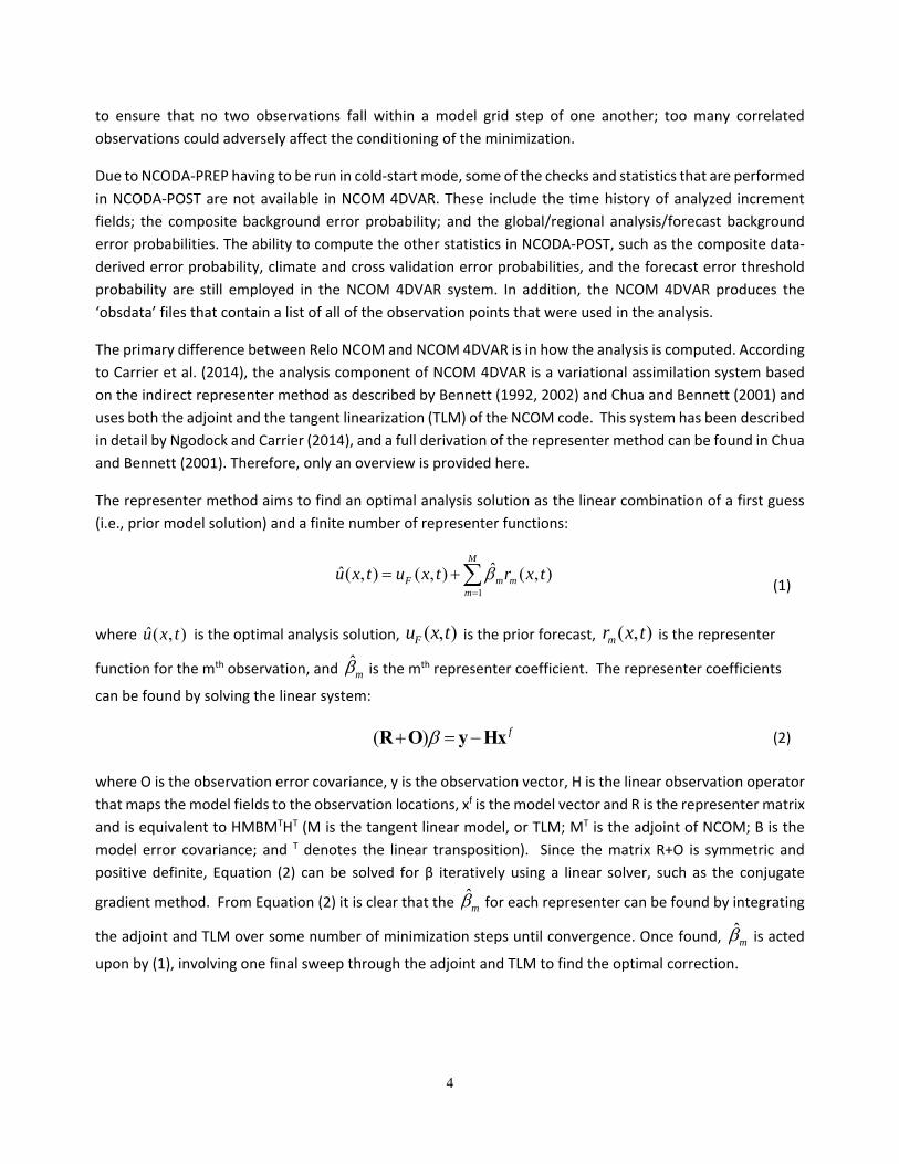
The representer method aims to find an optimal analysis solution as the linear combination of a first guess
(i.e., prior model solution) and a finite number of representer functions:
1
ˆˆ( , ) ( , ) ( , )M
F m mm
u x t u x t r x t
(1)
where ˆ( , )u x t is the optimal analysis solution, ( , )Fu x t is the prior forecast, ( , )mr x t is the representer
function for the mth observation, and ˆm is the mth representer coefficient. The representer coefficients
can be found by solving the linear system:
( ) f R O y Hx (2)
where O is the observation error covariance, y is the observation vector, H is the linear observation operator
that maps the model fields to the observation locations, xf is the model vector and R is the representer matrix
and is equivalent to HMBMTHT (M is the tangent linear model, or TLM; MT is the adjoint of NCOM; B is the
model error covariance; and T denotes the linear transposition). Since the matrix R+O is symmetric and
positive definite, Equation (2) can be solved for β iteratively using a linear solver, such as the conjugate
gradient method. From Equation (2) it is clear that the ˆm for each representer can be found by integrating
the adjoint and TLM over some number of minimization steps until convergence. Once found, ˆm is acted
upon by (1), involving one final sweep through the adjoint and TLM to find the optimal correction.
5
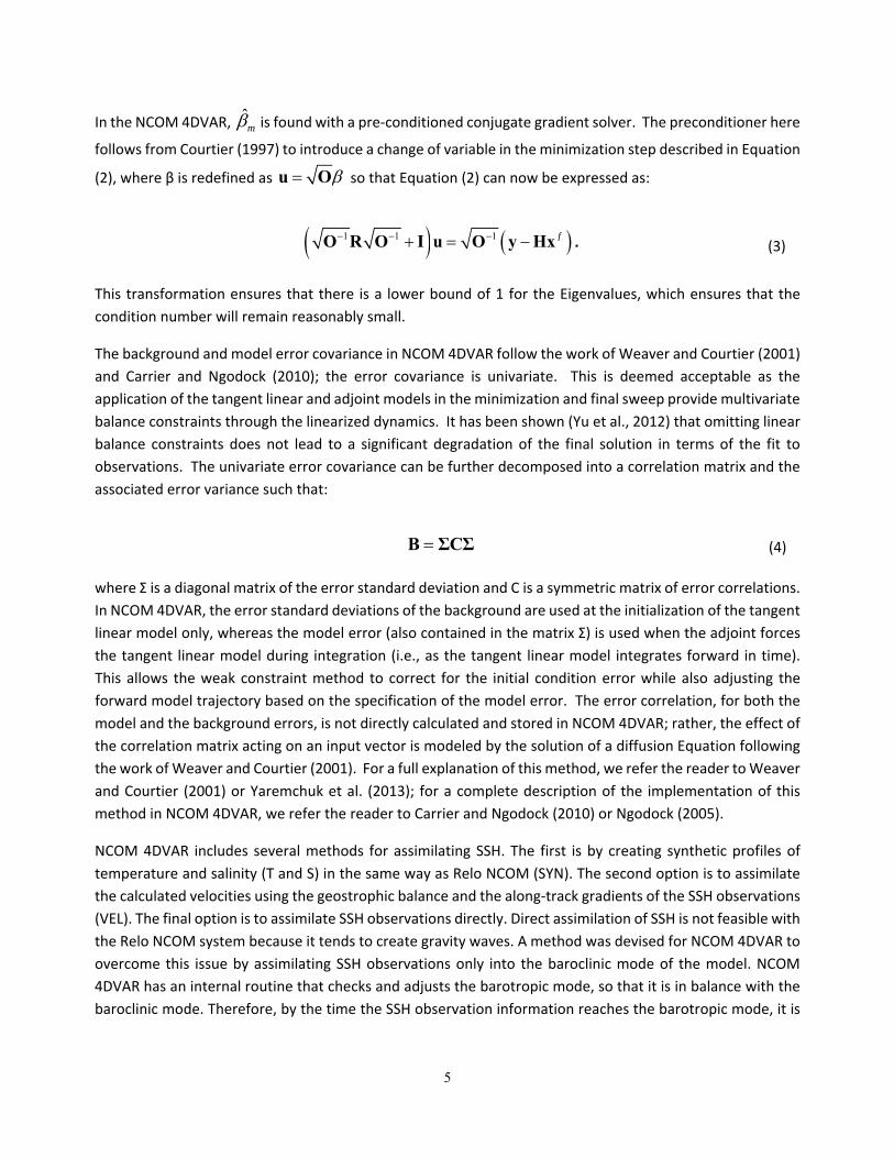
In the NCOM 4DVAR, ˆm is found with a pre‐conditioned conjugate gradient solver. The preconditioner here
follows from Courtier (1997) to introduce a change of variable in the minimization step described in Equation
(2), where β is redefined as u O so that Equation (2) can now be expressed as:
1 1 1 f O R O I u O y Hx . (3)
This transformation ensures that there is a lower bound of 1 for the Eigenvalues, which ensures that the
condition number will remain reasonably small.
The background and model error covariance in NCOM 4DVAR follow the work of Weaver and Courtier (2001)
and Carrier and Ngodock (2010); the error covariance is univariate. This is deemed acceptable as the
application of the tangent linear and adjoint models in the minimization and final sweep provide multivariate
balance constraints through the linearized dynamics. It has been shown (Yu et al., 2012) that omitting linear
balance constraints does not lead to a significant degradation of the final solution in terms of the fit to
observations. The univariate error covariance can be further decomposed into a correlation matrix and the
associated error variance such that:
B ΣCΣ (4)
where Σ is a diagonal matrix of the error standard deviation and C is a symmetric matrix of error correlations.
In NCOM 4DVAR, the error standard deviations of the background are used at the initialization of the tangent
linear model only, whereas the model error (also contained in the matrix Σ) is used when the adjoint forces
the tangent linear model during integration (i.e., as the tangent linear model integrates forward in time).
This allows the weak constraint method to correct for the initial condition error while also adjusting the
forward model trajectory based on the specification of the model error. The error correlation, for both the
model and the background errors, is not directly calculated and stored in NCOM 4DVAR; rather, the effect of
the correlation matrix acting on an input vector is modeled by the solution of a diffusion Equation following
the work of Weaver and Courtier (2001). For a full explanation of this method, we refer the reader to Weaver
and Courtier (2001) or Yaremchuk et al. (2013); for a complete description of the implementation of this
method in NCOM 4DVAR, we refer the reader to Carrier and Ngodock (2010) or Ngodock (2005).
NCOM 4DVAR includes several methods for assimilating SSH. The first is by creating synthetic profiles of
temperature and salinity (T and S) in the same way as Relo NCOM (SYN). The second option is to assimilate
the calculated velocities using the geostrophic balance and the along‐track gradients of the SSH observations
(VEL). The final option is to assimilate SSH observations directly. Direct assimilation of SSH is not feasible with
the Relo NCOM system because it tends to create gravity waves. A method was devised for NCOM 4DVAR to
overcome this issue by assimilating SSH observations only into the baroclinic mode of the model. NCOM
4DVAR has an internal routine that checks and adjusts the barotropic mode, so that it is in balance with the
baroclinic mode. Therefore, by the time the SSH observation information reaches the barotropic mode, it is
6
in dynamic balance with the model and does not produce gravity waves. A more detailed description of this
method is provided in Ngodock et al. (in press).
1.5 DocumentOverview
The NCOM 4DVAR system is an enhanced version of Relo NCOM, and has improved capabilities in limited
regional areas. Input data into NCOM 4DVAR comprises satellite and in situ observations from NAVOCEANO’s
operational data stream, along with initial and boundary conditions from either a larger Relo NCOM domain
or global HYCOM. This report provides the results of a series of validation experiments that compared the
prediction accuracy of NCOM 4DVAR version 1.0, relative to the current, operational version of Relo NCOM.
Validation metrics include: computational efficiency, the predictability of temperature and salinity, sonic
layer depth, and acoustic trapping through NCOM 4DVAR and Relo NCOM analyses, and ensuing model
forecasts. Metrics were computed using assimilated profile data, and in some experiments, non‐assimilated
glider and AXBT data. Overall, the validation results reveal that the applications of NCOM 4DVAR by itself
had an improved performance in terms of average RMS errors of temperature, salinity, velocity, and SSH
when compared to similar applications of NCODA‐VAR (in localized areas). The NCOM 4DVAR system is able
to produce an analysis that matches the available data, as well as produce an improved forecast as a result.
(Carrier et al., 2014)
The NCOM 4DVAR system has been validated and verified successfully for a number of field cases. These test
cases evaluated the analysis and prediction system’s ability to assimilate ocean data and produce an accurate
forecast. The test areas represented regions where significant variability and enough data existed to accurately
characterize the model. All of the experiments utilized a spherical grid projection and incorporated data from
NAVOCEANO’s decoded data stream that is processed by NCODA‐QC (Cummings, 2011) in near real time
(NRT). The NRT quality control (QC) decisions were used to select data for assimilation (Smith et al., 2012).
The user can refer to the NCOM 4DVAR Version 1.0 User’s Guide (Smith et al., in preparation) for further
details.
The validation experiments included the application of NCOM 4DVAR in the Okinawa Trough, Monterey Bay,
the Gulf of Mexico, the Pacific Rim of Hawaii, the Middle Atlantic Bight, Southern California, and the Kuroshio
Extension (Table 1‐1). Additional NCOM 4DVAR experiments for the Okinawa Trough, North Arabian Sea,
and US East Coast were performed in the same manner as the actual corresponding Relo NCOM runs were
performed operationally on the DoD Supercomputing Resource Center (DSRC) (Table 1‐1).
7
Table 1-1. Locations, dates, and types of data for NCOM 4DVAR validation tests. All experiments included assimilated observations from the NAVOCEANO operational QC data stream, as well as other data listed. The last three rows, (Okinawa Trough, North Arabian Sea, and US East Coast) were implemented at the DSRC (DoD Supercomputing Resource Center) in real-time operational mode.
LOCATION DATE OBSERVATIONAL DATA
LATTITUDE/LONGITUDE GRID
Okinawa Trough (OKT 07)
2007 SST, SSH, T/S (ARGO, XBT),
NAVOCEANO glider and
AXBTs (NOTE: Also
performed on the OOC)
17°N to 34°N and 118°E to 134°E 3 km horizontal, 50 vertical layers, 116 m depth, constant z‐levels extending max 5500 m
Monterey Bay (MB 03)
2003 SST, T/S (Gliders) 35.6°N to 37.49°N and 121.38°W to 123.2°W
2 km, 41 vertical layers
Gulf of Mexico (GOM12)
2012 SST, SSH, T/S (ARGO, XBT,),
Velocity (GLAD Drifting
Buoy), Direct SSH
18°N to 31°N and 79°W to 98°W 3.5 km horizontal (1/25°), 50 vertical levels
RIMPAC (RIMPAC 08)
2008 SST, SSH, T/S (ARGO, XBT),
4 Seagliders, 4 Slocum
gliders, CTDs
18°N to 24°N and 162°W to 154°W 3 km horizontal, 50 vertical levels
Mid Atlantic Bight 2011 Trident Warrior Exercise 39.5° N to 42° N and 69.5°E to 74.5°E
500 m horizontal 50 vertical levels
Southern California
2013 29° N to 44° N and 114°W to 129°W
3 km horizontal, 50 vertical layers
Kuroshio Extension
2010 31.1°N to 38.1°N and 137.1°E to 145.1° E
3 km horizontal, 50 vertical layers
Okinawa Trough 2014 17°N to 34°N and 118°E to 134°E 3 km horizontal, 50 vertical layers
North Arabian Sea
2014 19º to 31º N and 47º to 73º E 3 km horizontal, 50 vertical layers
US East Coast 2014 20°N to 42°N and 64°W to ‐82°W 3 km horizontal, 50 vertical layers

8
9
2.0 VALIDATIONMETRICS
2.1 Analysis/ForecastMetrics
Increase in forecast skill
Forecast accuracy measured using forecast‐observation differences with unassimilated observations
Comparisons of bias, RMS, and correlation coefficients
Comparison with independent data
Validation success was measured in the following areas:
Analysis and forecast accuracy of temperature and salinity was measured using forecast‐observation differences with both assimilated and unassimilated data. At the end of each analysis, and with 24‐hr forecasts (depending on the experiment), the model solution was compared to the data available during that portion of the analysis or forecast
The qualitative assessment of oceanographic realism and quality of the results were examined for each of the experiments. The analyses and forecasts of temperature, salinity, velocity (in both the horizontal and vertical), and SSH were examined to ensure that they were dynamically consistent and reasonable. This metric was performed by visually inspecting the solutions resulting from the different prediction systems for anomalous features such as significant localized biases or noisy vertical profiles
Metrics encompassing the testing of sound speed profiles, which include the predictability of sonic layer depth and acoustic trapping
2.2 EngineeringMetrics
• The computation time was recorded for all experiments to evaluate the overall efficiency of the prediction systems (A wallclock time of about one hour for each analysis/prediction cycle was recommended)
• The resource requirements (number of Central Processing Units‐CPUs, computer networking, etc…) are noted in this report (Table 5‐1)
• Robustness was tested by applying NCOM 4DVAR in multiple regions for multi‐month experiments • Resource requirements: The system needs to scale well with a targeted number of CPUs between
128 and 256 • User diagnostics and monitoring (NCOM 4DVAR should be able to successfully use the same
diagnostic tools that are currently used in NCODA‐VAR)
2.3 SubversionRepository
Developers at NRL regularly make changes, improvements, and bug fixes to the NCOM 4DVAR prediction
system, often concurrently. Therefore, a subversion repository (http://subversion.tigris.org/; Collins‐
Sussman et al., 2007) has been created at NRL Stennis Space Center (NRLSSC), wherein different versions of
NCOM 4DVAR, and its complete developmental history, are stored and available for user access. The official

10
version of NCOM 4DVAR used in this validation test report is located in the NRLSSC repository and can be
accessed at the following internet addresses:
https://www7320.nrlssc.navy.mil/svn/repos/NCOM/branches/4.3/
https://www7320.nrlssc.navy.mil/svn/repos/RELO/branches/4dvar/.
The first repository link above includes all of the NCOM code. All of the components of the NCOM 4DVAR,
including the adjoint, TLM, and the solver have been merged with the main NCOM branch. The second
repository link contains the version of Relo scripts that are needed to operate and cycle the NCOM 4DVAR.
The NRL subversion repository is accessible to select DoD IP addresses outside the NRLSSC system, such as
the High Performance Computing Modernization Program (HPCMP) DoD Supercomputing Resource Center
DSRC) platforms.
The Relo NCOM with NCODA‐VAR software that was used for comparison can be obtained at:
http://www7320.nrlssc.navy.mil/svn/repos/RELO/branches/3DVAR.
11
3.0 VALIDATIONTESTDESCRIPTIONANDRESULTS:OKINAWATROUGH
The Okinawa Trough (OT) region is highly dynamic in nature; it has a complex geometry, sharp bathymetry
gradient, a strong Kuroshio current, large barotropic and internal tides, and frequent typhoon passage. All of
these features provide an excellent opportunity to evaluate air‐ocean‐wave interactions (Smith et al., 2012).
3.1 TestAreaandObservations:OkinawaTrough The Okinawa Trough domain was chosen as a validation test area for two reasons. First, a Navy exercise was
conducted in the fall of 2007; it provided a large data set of AXBT and glider profile observations useful for
assimilation and validation purposes. It is beneficial to have a large data set of profile observations to validate
NCOM 4DVAR’s capability to project sea surface information into the interior of the ocean. Secondly, this
region is dynamically rich with the Kuroshio Current and the meandering eddies it sheds. Additionally,
significant river input, large tidal amplitudes, and internal tide generation contribute to a comprehensive
examination of the predictive capability of the analysis/forecasting systems (Smith et al., 2012).
The Okinawa Trough is located between Taiwan and southern Japan and is a seabed feature of the East China
Sea; it is an active, initial back‐arc rifting basin which formed behind the Ryukyu arc‐trench system in the
western Pacific Ocean. It has a large section more than 3,300 feet (1,000 meters‐m) deep and a maximum
depth of 8,912 feet (2,716 m) (Smith et al., 2012). The study region encompassed both the Okinawa Trough
and Ryukyu Islands of Japan, from 17°N to 34°N and 118°E to 134°E (Figure 3‐1) (Smith et al., 2012).
Observational data came from several sources. In 2007, over 7000 subsurface in situ temperature (T) and
salinity (S) profiles, along with 1400 subsurface T and S profiles (from the World Meteorological Organization
Global Telecommunications System ‐ WMO GTS) were collected (Barron et al., 2010). Altimetry data came
from Global Telecommunications System (GTS) and the remotely sensed SST data came from ENVISAT
(European Space Agency ‐ ENVIronmental SATellite) satellites. Glider data and AXBT observations were
provided courtesy of NAVOCEANO (Smith et al., 2012).
12
Figure 3-1. The Okinawa Trough model domain, with 3 km horizontal resolution. The study region encompassed both the Okinawa Trough and Ryukyu Islands of Japan, from 17°N to 34°N and 118°E to 134°E.
3.2 ModelSetup:OkinawaTrough
3.2.1 Experiment Overview
The following Okinawa Trough experiments involve twelve‐month (2007) implementations of RELO NCOM
and NCOM 4DVAR. Each of these experiments used surface boundary conditions from the 0.5⁰ NOGAPS,
lateral boundary conditions from a 6 km Relo NCOM (that was nested within the global NCOM), and had 50
layers in the vertical with 25 free‐sigma levels extending to a depth of 116 meters with constant z‐levels
extending down to a maximum of 5500 meters.
Four one‐year cycling assimilation‐forecast runs were made with this domain and included: (1) a standard
Relo NCOM run using the operational implementation of NCODA‐VAR; (2) the NCOM 4DVAR analysis system
where the SSH observations were included via synthetic profiles of temperature and salinity generated by
the Modular Ocean Data Assimilation System (MODAS); (3) NCOM 4DVAR that included SSH observations by
transforming the SSH values into along‐track height gradients (i.e., geostrophic velocities); and (4) NCOM
4DVAR that included SSH observations through direct assimilation of the along‐track measurements. (See
Section 1.4 for a description of the SSH assimilation methods.) The three different methods of SSH
assimilation were tested to determine the best method for the NCOM 4DVAR within this region. The
standard implementation of NCODA‐VAR utilizes the MODAS synthetic profiles; NCODA‐VAR is capable of
assimilating derived velocities and direct measurements of SSH (this was not tested because these do not
13
represent the operational configuration). For the 4DVAR assimilation of along‐track SSH, an estimated mean
SSH field was needed to transform the observations from height anomalies into the form of the ocean model.
For this, a multi‐year mean SSH field from the HYbrid Coordinate Ocean Model (HYCOM) was interpolated to
the observation locations and added prior to the inclusion of the data within the assimilation.
The operation of the NCOM 4DVAR software is very similar to that of the Relo NCOM; most of the parameter
files are the same, with only a handful of parameters that need to be added or changed to run NCOM 4DVAR.
A list of the parameters from the two primary namelist files (relo.env and relo.nl) that were used in this
experiment is provided in the Appendix (Section 11). For clarity, the parameters that have been added or
changed from the operational Relo NCOM setup are bolded. For more specific details on specifying these
parameters, the NCOM 4DVAR Version 1.0 User’s Guide (Smith et al., in prep).
3.2.2 Domain Details
At 3 kilometers (km) resolution, the Okinawa Trough domain has a spatial size of 535 by 628 grid points and
50 layers; this corresponds to a total of 16,799,000 grid points. Due to the computational cost of NCOM
4DVAR, which involves solving the adjoint (AD) and tangent linear models (TLM) several times within the
minimization driver, the total time to run the assimilation for a model grid of this size is operationally
prohibitive.
To reduce the computational time it is necessary to run the NCOM 4DVAR assimilation on a reduced
resolution grid. For the Okinawa Trough experiments, the model grid was coarsened by interpolating the 3
km model background to a 6 km analysis grid that covered the same region and vertical structure as the
original configuration. This is deemed acceptable as the static spatial covariance scales employed by the
NCOM 4DVAR are based on the Rossby radius of deformation, which for this region is approximately 40 km.
Once the assimilation is completed on the reduced‐grid, the analysis increments are projected back to the
original 3 km resolution and added to the full‐resolution background state to produce the analysis. A series
of experiments conducted during the early testing phase for the NCOM 4DVAR in the Okinawa Trough
confirmed that a forecast run at 3 km initialized by a 6 km analysis yields a nearly identical solution as one
run from a 3 km analysis. This result, coupled with the fact that the computational cost of the analysis is
greatly reduced by the use of the coarse‐resolution analysis, justifies this method.
3.2.3 Experiment Objectives
Three main objectives were specified for the twelve‐month Okinawa Trough experiment: (1) test the direct
SSH assimilation; (2) directly compare the 24‐hr forecasts initialized by the 3DVAR and 4DVAR analysis
systems; and (3) identify any model‐drift that may be present in the cycling forecast from the 4DVAR analysis
(due to the assimilation method, specifically the assimilation of along‐track SSH). The latter objective is based
on the concern that the assimilation of along‐track SSH may produce unrealistic corrections to the
thermodynamic state of the model. This is not a concern when synthetic profiles are assimilated, as the
generation of these profiles uses climatology to constrain the temperature and salinity profiles. This
climatological constraint does not exist when SSH observations are assimilated directly via the 4DVAR. On
the other hand, the 4DVAR does constrain the adjustments to the temperature and salinity by the
14
background around which the AD and TLM models are linearized. The objective is to determine if this
constraint is sufficient to prevent unrealistic adjustments to the thermodynamic structure and, therefore,
prevent the model solution from drifting far from reality.
In addition to the 12‐month experiments, several three‐month experiments were performed during the same
time period of the Navy exercise; many T and S profile observations were collected. These short term
experiments were performed to examine longer forecasts (out to 72 hours) to see how long the corrections
in the NCOM 4DVAR analysis persisted in the model. Also, various observation types were withheld from the
assimilation and used for independent validation.
3.3 Results:OkinawaTrough
Before evaluating the forecast solutions initialized by the NCOM 4DVAR, it is important to confirm that the
assimilation procedure is functioning properly. To that end, a series of statistical evaluations were made of
the NCOM 4DVAR analysis and resulting forecast, using observations as a measure of truth. Figure 3‐2
illustrates a global fit (space and time) of the background (black) and the NCOM 4DVAR analysis (white) to
the assimilated observations for the entire 12‐month run, as a function of the number of standard deviations
of the prescribed observation error for the version of NCOM 4DVAR assimilating synthetic profiles (referred
to as 4DVAR SYN).
Figure 3-2. Global Fit (space and time) of the 24-hr forecast (black) and the analysis (white) of the 4DVAR SYN to the assimilated observations of temperature (left) and salinity (right) for the 12-month Okinawa Trough run, as a function of the number of standard deviations of the prescribed observation error. There is no boxplot for SSH, since direct SSH observations were not assimilated.
15
It is assumed that a properly‐functioning variational analysis system should fit 90% of the observations to
within two standard deviations of the observation error. This is the case for the 4DVAR SYN experiment
(Figure 3‐2), as the analysis fits roughly 78% (96%) of the temperature observations within one (two)
standard deviations (left panel) and 87% (98%) of the salinity observations within one (two) standard
deviations. Similar results are seen for the 4DVAR that employs direct assimilation of SSH observations
(here after referred to as 4DVAR SSH) (Figure 3‐3). Once again, the overall fit of temperature and salinity is
well within an acceptable range. Since SSH observations were assimilated, this comparison also shows the
SSH fit, which indicates that the 4DVAR SSH analysis is fitting 60% (88%) of the SSH observations to within
one (two) standard deviations. The 88% fit falls just short of the specified criteria, which indicates that the
prescribed initial condition and model error values within the error covariance may need to be tuned
further to produce an improved fit. However, there is a significant improvement over the background fit
and, as will be shown later, this does not impact the ability of 4DVAR SSH to produce a superior SSH
forecast than the solution initialized by Relo NCOM.
Figure 3-3. Global Fit (space and time) of the 24-hr forecast (black) and the analysis (white) of 4DVAR SSH to the assimilated observations of temperature (left), salinity (middle), and SSH (right) for the 12-month Okinawa Trough run, as a function of the number of standard deviations of the prescribed observation error.
16
Figure 3‐4 shows the same observation fit bar chart as Figure 3‐3, but this experiment used derived
geostrophic velocities (referred to as 4DVAR VEL). As with Figures 3‐2 and 3‐3, this comparison demonstrates
that the 4DVAR VEL experiment fits the temperature and salinity observations well. Figure 3‐4 also shows
the fit to the derived velocity observations. The prior (background) and posterior fit to velocity are nearly
identical, but both very high with fits around 80% (98%) within one (two) standard deviations. This is likely
due to the high observation error assigned the derived velocity measurements by the NCODA data
preparation suite, which is responsible for converting the SSH along‐track gradients to geostrophic velocities.
This indicates that this data are not likely to have much impact on the correction, and therefore, the data are
not constraining the mesoscale, as well as the direct and synthetic methods; this will become apparent later
in this evaluation.
Figure 3-4. Same as Figure 3-3, except for the 4DVAR VEL 12-month Okinawa Trough experiment, which assimilated derived geostrophic velocities instead of assimilating SSH directly. Therefore, the right boxplot is for velocity (VEL) instead of SSH.
17
3.3.1 Time Distribution of Errors
The previous evaluation showed overall global fits in time and space; it is also important to see if there is any
seasonality in the analysis fit (and the corresponding 24‐hr forecast that is generated). To do this, a statistical
measure of the fit of the analysis and 24‐hr forecast to available observations as a function of time is
computed. This evaluation can also help determine if any model drift is present in the solution; this would
manifest itself as increasing 24‐hr forecast error with time (as the model solution slowly drifts from reality
over time). The statistical measure employed for this is a normalized mean absolute error that will be
referred to as the Jfit measure. The Jfit measure is computed as,
1
1 Mm m
fitm m
y H xJ
M
(5)
where M is the total number of observations; ym, Hm, and σm are the observation, observation operator, and
observation error, respectively, associated with the mth observation; and x is the model state (either the
forecast or analysis). Equation 5 indicates that if the forecast or analysis fits the collective observations within
their corresponding prescribed observation errors, the Jfit value will be at or below one. If the Jfit value is well
below the value of one, then this may indicate that the solution is over‐fitting the observations, and the
prescribed model errors should be reduced.
Figure 3‐5 shows the Jfit value (labeled error on the plot) for the 4DVAR SYN experiment from 15 January
through 31 December, 2007 for temperature (top panel) and salinity (bottom panel) with the First Guess (the
previous cycle’s 24‐hr forecast) shown in black and the 4DVAR analysis in red. The Jfit value for temperature
does not indicate any seasonality of the analysis or first guess fit to the available observations, nor does the
error in the first guess rise with each cycle through time; rather, the analysis fits the available observations
generally within the prescribed error (1.0) and the trend in the first guess error remains relatively flat with
time (with values between 1.0 and 2.0 for the entire year). This is consistent with the assumption that the
assimilation of synthetic profiles does not induce model drift. The salinity results are generally the same,
except with larger variability and slightly higher magnitudes in both the first guess and analysis error. There
are a few cycles where the salinity analysis error is well above 1.0; further analysis indicates that the number
of salinity observations drop significantly at these times. It is probable that at these times the gradient of the
cost function being minimized is dominated by the larger number of temperature observations (specifically,
sea surface temperature). To reduce computational time, the minimization driver is capped to a maximum
of ten iterations. Due to this, the minimization did not fully converge for the salinity analysis; this would likely
be helped by either reducing the number of SST observations or by increasing the number of minimization
iterations in the conjugate gradient solver. However, the NCOM 4DVAR corrects these large spikes rather
quickly. Overall, the analysis errors are significantly less than those for the first guess solution and, for the
most part, are less than one. This means the analysis is fitting within the observation error.
18
Figure 3-5. Errors in temperature (top) and salinity (bottom) solutions from the first guess (black) and the analysis (red) relative to the observations that were assimilated for the 4DVAR SYN experiment. Since SSH observations were not assimilated directly, there is no error plot for SSH. These errors span the entire year of the Okinawa Trough experiment (15 January through 31 December 2007) and are normalized by the corresponding observation error (Jfit, see Equation 5).
Figure 3‐6 shows the same Jfit value as in Figure 3‐5, but for the 4DVAR SSH experiment. An additional panel
is added to Figure 3‐6 that shows the Jfit value for the SSH observations (that were directly assimilated). The
temperature and salinity results are generally the same between the 4DVAR SSH and 4DVAR SYN
experiments, with one difference regarding the temperature analysis. On 18 August 2007, the analysis for
the temperature field in the 4DVAR SSH analysis exhibited an unusually high Jfit value. Examination of the
results indicates that this is due to a combination of a large number of temperature innovations that were
particularly high (> 5.0 degrees) and the aforementioned limited minimization iteration number. The
temperature analysis did not converge within the prescribed iteration maximum; as such, some of the
analysis increments were not sufficiently large enough to reduce the misfit between the model and
observations. Again, this could be alleviated by increasing the number of iterations in the conjugate gradient
or by reducing the number of large‐innovation temperature misfits allowed in the analysis cycle. The result
shown here is deemed acceptable as it is the only occurrence within the 12‐month time period.
Examining the fit to SSH (Figure 3‐6, bottom panel) shows that the analysis generally fits the SSH observations
within the prescribed observation error, except at a few times throughout the year. These higher Jfit values
correspond to times when the amount of available SSH observations is much lower (similar to what has
occurred with the salinity analysis). As in the salinity analysis, the lack of fit to SSH is likely due to the
combination of the relatively higher number of temperature observations and the iteration cap for the
conjugate gradient algorithm.
19
Figure 3-6. Errors in temperature (top), salinity (middle), and SSH (bottom) solutions from the first guess (black) and the analysis (red) relative to the observations that were assimilated for the 4DVAR SSH experiment, which assimilated SSH directly. These errors span the entire year of the Okinawa Trough experiment (15 January through 31 December 2007) and are normalized by the corresponding observation error (Equation 5).
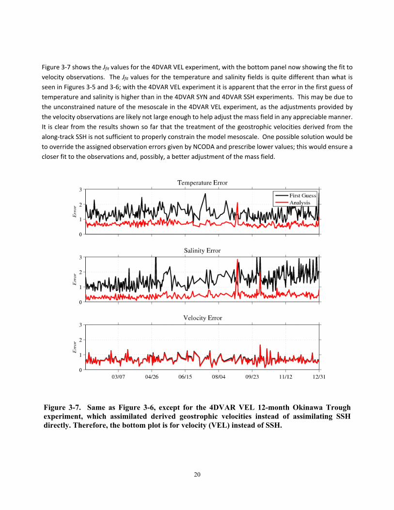
20
Figure 3‐7 shows the Jfit values for the 4DVAR VEL experiment, with the bottom panel now showing the fit to
velocity observations. The Jfit values for the temperature and salinity fields is quite different than what is
seen in Figures 3‐5 and 3‐6; with the 4DVAR VEL experiment it is apparent that the error in the first guess of
temperature and salinity is higher than in the 4DVAR SYN and 4DVAR SSH experiments. This may be due to
the unconstrained nature of the mesoscale in the 4DVAR VEL experiment, as the adjustments provided by
the velocity observations are likely not large enough to help adjust the mass field in any appreciable manner.
It is clear from the results shown so far that the treatment of the geostrophic velocities derived from the
along‐track SSH is not sufficient to properly constrain the model mesoscale. One possible solution would be
to override the assigned observation errors given by NCODA and prescribe lower values; this would ensure a
closer fit to the observations and, possibly, a better adjustment of the mass field.
Figure 3-7. Same as Figure 3-6, except for the 4DVAR VEL 12-month Okinawa Trough experiment, which assimilated derived geostrophic velocities instead of assimilating SSH directly. Therefore, the bottom plot is for velocity (VEL) instead of SSH.
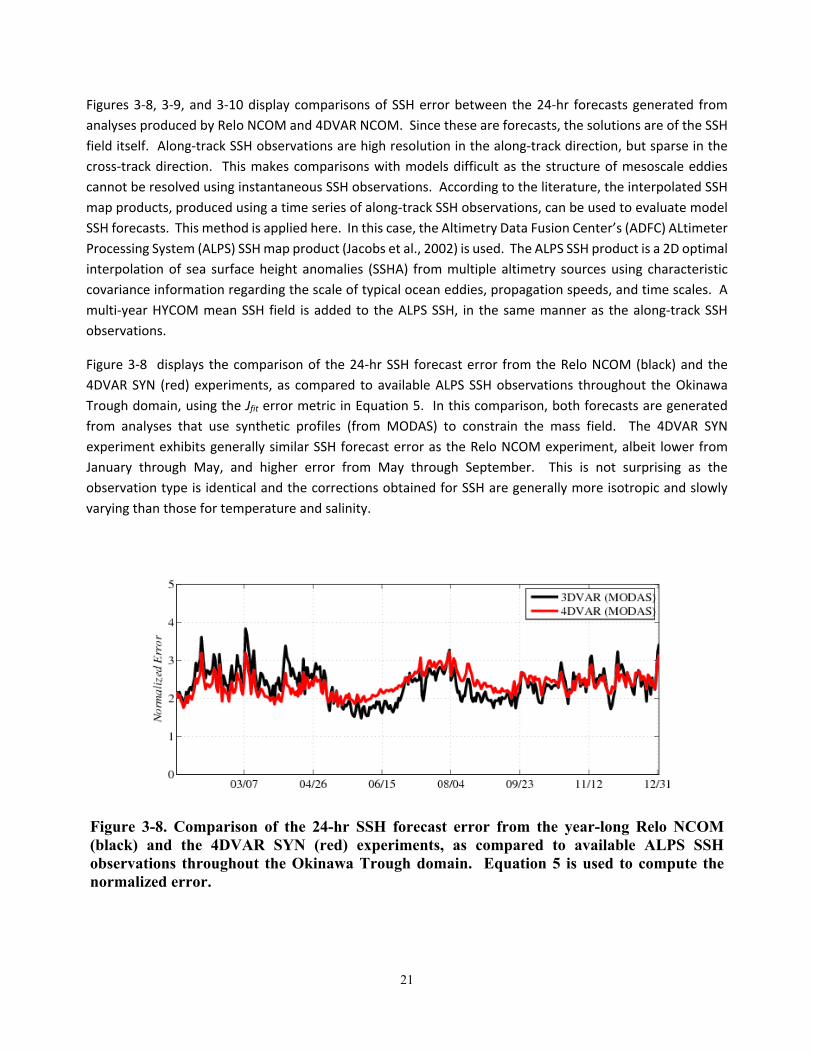
21
Figures 3‐8, 3‐9, and 3‐10 display comparisons of SSH error between the 24‐hr forecasts generated from
analyses produced by Relo NCOM and 4DVAR NCOM. Since these are forecasts, the solutions are of the SSH
field itself. Along‐track SSH observations are high resolution in the along‐track direction, but sparse in the
cross‐track direction. This makes comparisons with models difficult as the structure of mesoscale eddies
cannot be resolved using instantaneous SSH observations. According to the literature, the interpolated SSH
map products, produced using a time series of along‐track SSH observations, can be used to evaluate model
SSH forecasts. This method is applied here. In this case, the Altimetry Data Fusion Center’s (ADFC) ALtimeter
Processing System (ALPS) SSH map product (Jacobs et al., 2002) is used. The ALPS SSH product is a 2D optimal
interpolation of sea surface height anomalies (SSHA) from multiple altimetry sources using characteristic
covariance information regarding the scale of typical ocean eddies, propagation speeds, and time scales. A
multi‐year HYCOM mean SSH field is added to the ALPS SSH, in the same manner as the along‐track SSH
observations.
Figure 3‐8 displays the comparison of the 24‐hr SSH forecast error from the Relo NCOM (black) and the
4DVAR SYN (red) experiments, as compared to available ALPS SSH observations throughout the Okinawa
Trough domain, using the Jfit error metric in Equation 5. In this comparison, both forecasts are generated
from analyses that use synthetic profiles (from MODAS) to constrain the mass field. The 4DVAR SYN
experiment exhibits generally similar SSH forecast error as the Relo NCOM experiment, albeit lower from
January through May, and higher error from May through September. This is not surprising as the
observation type is identical and the corrections obtained for SSH are generally more isotropic and slowly
varying than those for temperature and salinity.
Figure 3-8. Comparison of the 24-hr SSH forecast error from the year-long Relo NCOM (black) and the 4DVAR SYN (red) experiments, as compared to available ALPS SSH observations throughout the Okinawa Trough domain. Equation 5 is used to compute the normalized error.
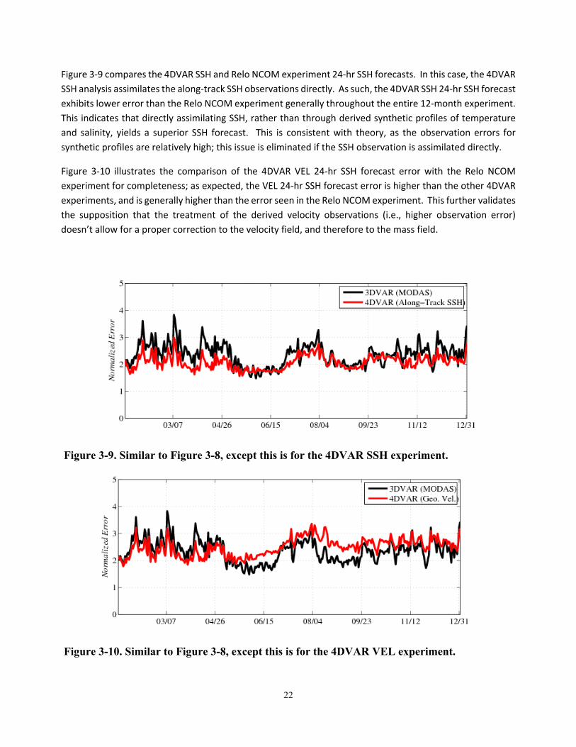
22
Figure 3‐9 compares the 4DVAR SSH and Relo NCOM experiment 24‐hr SSH forecasts. In this case, the 4DVAR
SSH analysis assimilates the along‐track SSH observations directly. As such, the 4DVAR SSH 24‐hr SSH forecast
exhibits lower error than the Relo NCOM experiment generally throughout the entire 12‐month experiment.
This indicates that directly assimilating SSH, rather than through derived synthetic profiles of temperature
and salinity, yields a superior SSH forecast. This is consistent with theory, as the observation errors for
synthetic profiles are relatively high; this issue is eliminated if the SSH observation is assimilated directly.
Figure 3‐10 illustrates the comparison of the 4DVAR VEL 24‐hr SSH forecast error with the Relo NCOM
experiment for completeness; as expected, the VEL 24‐hr SSH forecast error is higher than the other 4DVAR
experiments, and is generally higher than the error seen in the Relo NCOM experiment. This further validates
the supposition that the treatment of the derived velocity observations (i.e., higher observation error)
doesn’t allow for a proper correction to the velocity field, and therefore to the mass field.
Figure 3-9. Similar to Figure 3-8, except this is for the 4DVAR SSH experiment.
Figure 3-10. Similar to Figure 3-8, except this is for the 4DVAR VEL experiment.
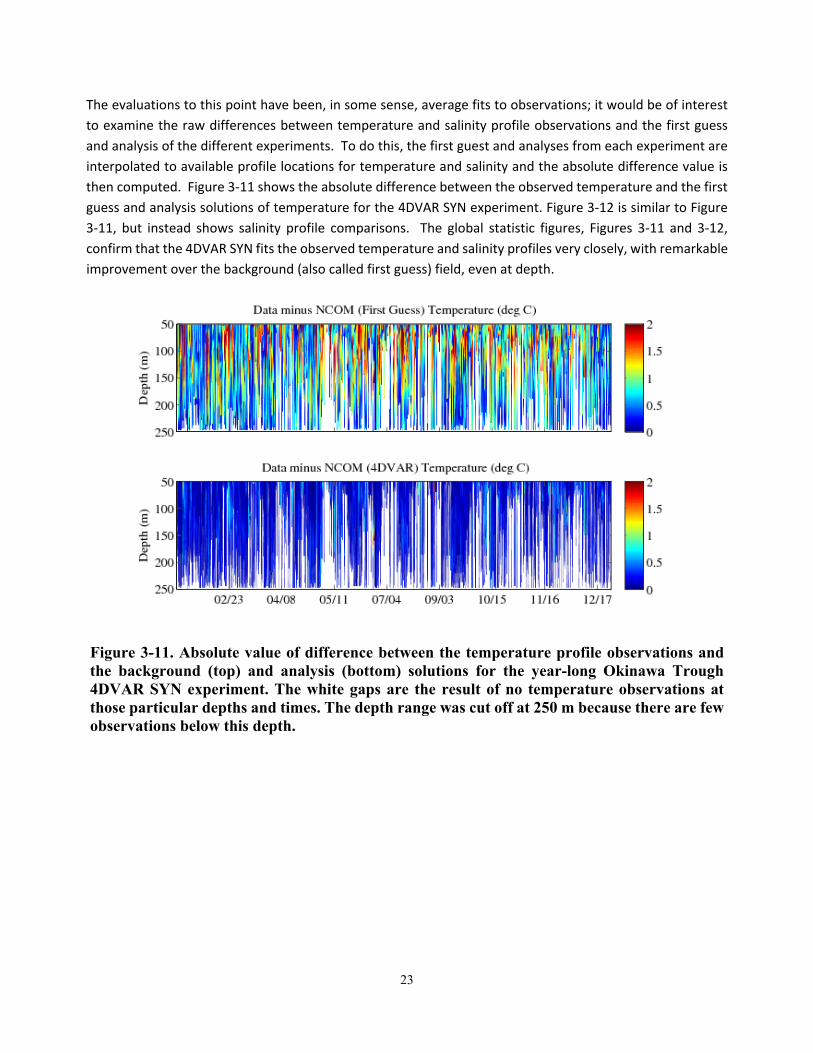
23
The evaluations to this point have been, in some sense, average fits to observations; it would be of interest
to examine the raw differences between temperature and salinity profile observations and the first guess
and analysis of the different experiments. To do this, the first guest and analyses from each experiment are
interpolated to available profile locations for temperature and salinity and the absolute difference value is
then computed. Figure 3‐11 shows the absolute difference between the observed temperature and the first
guess and analysis solutions of temperature for the 4DVAR SYN experiment. Figure 3‐12 is similar to Figure
3‐11, but instead shows salinity profile comparisons. The global statistic figures, Figures 3‐11 and 3‐12,
confirm that the 4DVAR SYN fits the observed temperature and salinity profiles very closely, with remarkable
improvement over the background (also called first guess) field, even at depth.
Figure 3-11. Absolute value of difference between the temperature profile observations and the background (top) and analysis (bottom) solutions for the year-long Okinawa Trough 4DVAR SYN experiment. The white gaps are the result of no temperature observations at those particular depths and times. The depth range was cut off at 250 m because there are few observations below this depth.
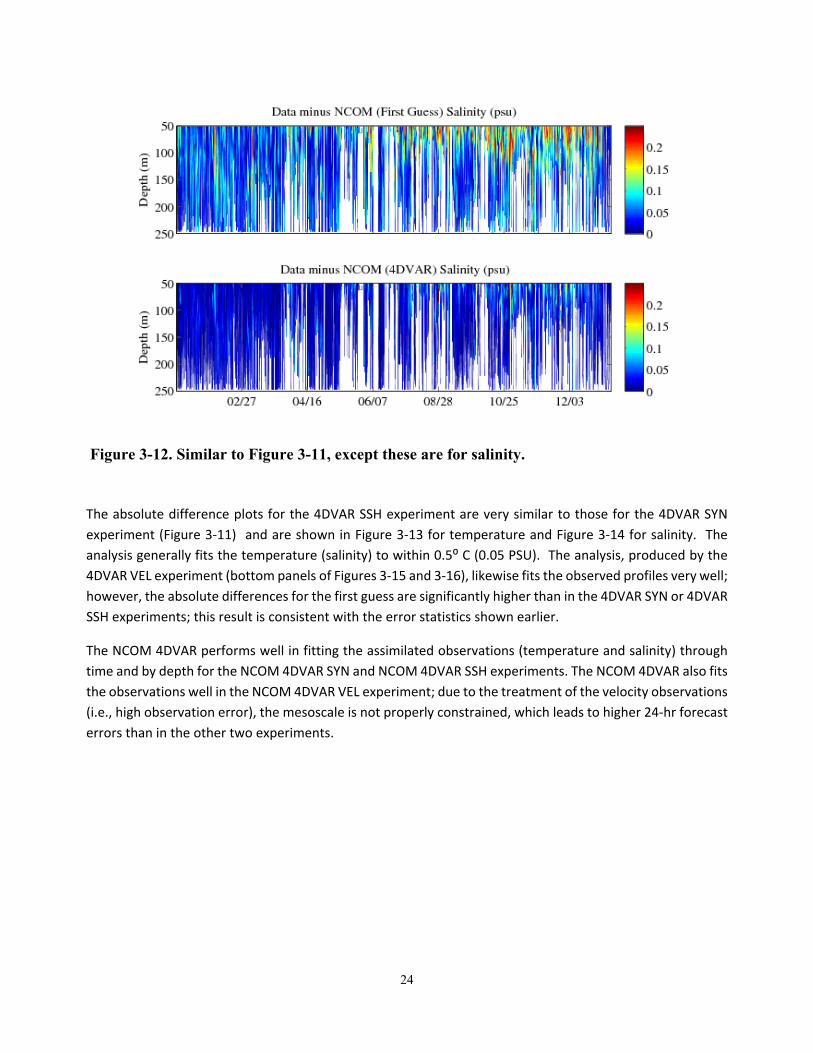
24
Figure 3-12. Similar to Figure 3-11, except these are for salinity.
The absolute difference plots for the 4DVAR SSH experiment are very similar to those for the 4DVAR SYN
experiment (Figure 3‐11) and are shown in Figure 3‐13 for temperature and Figure 3‐14 for salinity. The
analysis generally fits the temperature (salinity) to within 0.5⁰ C (0.05 PSU). The analysis, produced by the
4DVAR VEL experiment (bottom panels of Figures 3‐15 and 3‐16), likewise fits the observed profiles very well;
however, the absolute differences for the first guess are significantly higher than in the 4DVAR SYN or 4DVAR
SSH experiments; this result is consistent with the error statistics shown earlier.
The NCOM 4DVAR performs well in fitting the assimilated observations (temperature and salinity) through
time and by depth for the NCOM 4DVAR SYN and NCOM 4DVAR SSH experiments. The NCOM 4DVAR also fits
the observations well in the NCOM 4DVAR VEL experiment; due to the treatment of the velocity observations
(i.e., high observation error), the mesoscale is not properly constrained, which leads to higher 24‐hr forecast
errors than in the other two experiments.
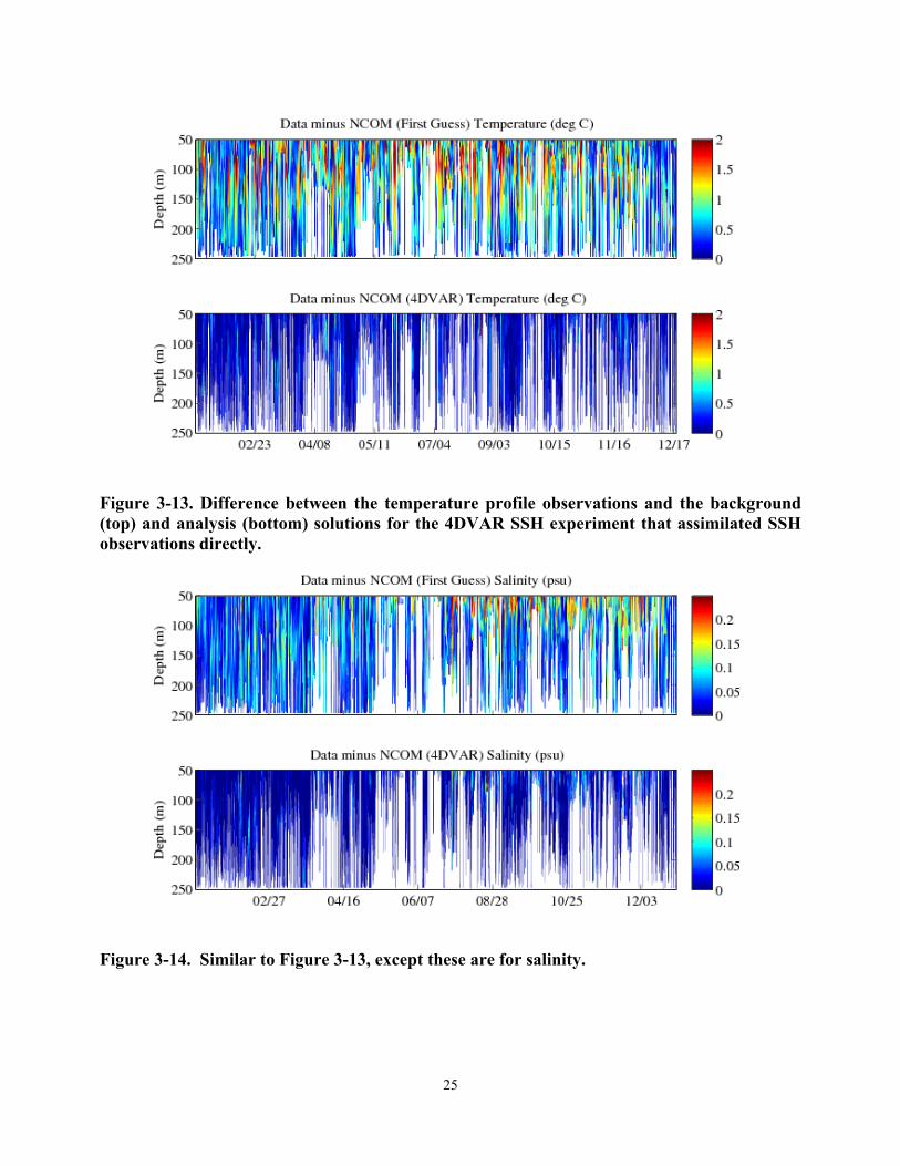
25
Figure 3-13. Difference between the temperature profile observations and the background (top) and analysis (bottom) solutions for the 4DVAR SSH experiment that assimilated SSH observations directly.
Figure 3-14. Similar to Figure 3-13, except these are for salinity.
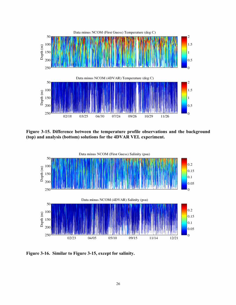
26
Figure 3-15. Difference between the temperature profile observations and the background (top) and analysis (bottom) solutions for the 4DVAR VEL experiment.
Figure 3-16. Similar to Figure 3-15, except for salinity.
27
3.3.2 Profile Distribution Errors
A comparison between the forecasts of the subsurface generated from the analyses produced by the NCOM
4DVAR and 3DVAR will now be made. The subsurface thermodynamic characteristics should be captured by
the model, thus the first comparison presented is the RMS errors computed as a function of depth, rather
than time. This error metric, computed for the forecasts generated from the Relo NCOM and NCOM 4DVAR
analyses, presents a comparison of the model layer‐by‐layer error (relative to available profile observations).
Figure 3‐17 shows the profile of RMS errors for the 24‐hr forecasts computed from the 12‐month runs of the
4DVAR SYN (red), 4DVAR SSH (blue), 4DVAR VEL (green) and the Relo NCOM (black) experiments for
temperature (left panel) and salinity (right panel) relative to profile observations. The value (N) in the left
panel is the total number of profiles used to compute these statistics during the 12‐month time period. Each
profile consisted of both temperature and salinity observations down to a particular depth, so the total
number of temperature and salinity observations used in these comparisons is the same. NCODA‐QC
computed synthetic salinity profiles using MODAS for profile observations of just temperature (such as
AXBTs).
It should be noted that not all of the profiles used for these comparisons went down to below 1400 m and
many were confined to within the upper 100 m. The three 4DVAR experiments in Figure 3‐17 have similar
profile error statistics and all of them outperform the Relo NCOM, except for salinity between 200 – 350 m
depth.
The profile RMS errors for the temperature field shows that the 24‐hr forecasts from the NCOM 4DVAR
experiments and Relo NCOM are fairly similar in the upper most 50 m, but between 50 m and 500 m, the
error in the NCOM 4DVAR forecasts are much lower than in the Relo NCOM experiment; below 500 m, the
errors begin to converge again.
The result from the salinity comparison is quite different, as the NCOM 4DVAR forecasts have significantly
lower error in the upper 50 m, but are similar to Relo NCOM below this level. For the model levels with the
highest observation density (< 100 m depth), the NCOM 4DVAR forecasts are better than Relo NCOM for both
temperature and salinity.
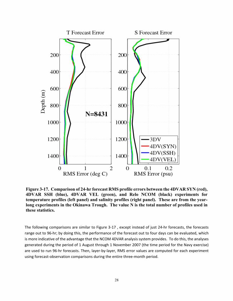
28
Figure 3-17. Comparison of 24-hr forecast RMS profile errors between the 4DVAR SYN (red), 4DVAR SSH (blue), 4DVAR VEL (green), and Relo NCOM (black) experiments for temperature profiles (left panel) and salinity profiles (right panel). These are from the year-long experiments in the Okinawa Trough. The value N is the total number of profiles used in these statistics.
The following comparisons are similar to Figure 3‐17 , except instead of just 24‐hr forecasts, the forecasts
range out to 96‐hr; by doing this, the performance of the forecast out to four days can be evaluated, which
is more indicative of the advantage that the NCOM 4DVAR analysis system provides. To do this, the analyses
generated during the period of 1 August through 1 November 2007 (the time period for the Navy exercise)
are used to run 96‐hr forecasts. Then, layer‐by‐layer, RMS error values are computed for each experiment
using forecast‐observation comparisons during the entire three‐month period.
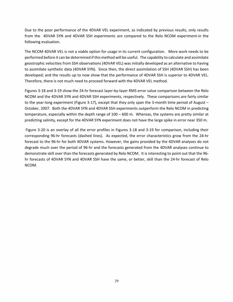
29
Due to the poor performance of the 4DVAR VEL experiment, as indicated by previous results, only results
from the 4DVAR SYN and 4DVAR SSH experiments are compared to the Relo NCOM experiment‐in the
following evaluation.
The NCOM 4DVAR VEL is not a viable option for usage in its current configuration. More work needs to be
performed before it can be determined if this method will be useful. The capability to calculate and assimilate
geostrophic velocities from SSH observations (4DVAR VEL) was initially developed as an alternative to having
to assimilate synthetic data (4DVAR SYN). Since then, the direct assimilation of SSH (4DVAR SSH) has been
developed; and the results up to now show that the performance of 4DVAR SSH is superior to 4DVAR VEL.
Therefore, there is not much need to proceed forward with the 4DVAR VEL method.
Figures 3‐18 and 3‐19 show the 24‐hr forecast layer‐by‐layer RMS error value comparison between the Relo
NCOM and the 4DVAR SYN and 4DVAR SSH experiments, respectively. These comparisons are fairly similar
to the year‐long experiment (Figure 3‐17), except that they only span the 3‐month time period of August –
October, 2007. Both the 4DVAR SYN and 4DVAR SSH experiments outperform the Relo NCOM in predicting
temperature, especially within the depth range of 100 – 600 m. Whereas, the systems are pretty similar at
predicting salinity, except for the 4DVAR SYN experiment does not have the large spike in error near 350 m.
Figure 3‐20 is an overlay of all the error profiles in Figures 3‐18 and 3‐19 for comparison, including their
corresponding 96‐hr forecasts (dashed lines). As expected, the error characteristics grow from the 24‐hr
forecast to the 96‐hr for both 4DVAR systems. However, the gains provided by the 4DVAR analyses do not
degrade much over the period of 96‐hr and the forecasts generated from the 4DVAR analyses continue to
demonstrate skill over than the forecasts generated by Relo NCOM. It is interesting to point out that the 96‐
hr forecasts of 4DVAR SYN and 4DVAR SSH have the same, or better, skill than the 24‐hr forecast of Relo
NCOM.
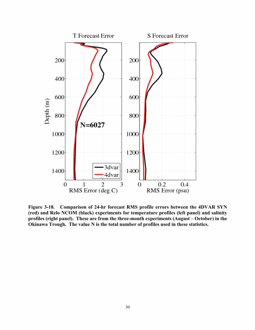
30
Figure 3-18. Comparison of 24-hr forecast RMS profile errors between the 4DVAR SYN (red) and Relo NCOM (black) experiments for temperature profiles (left panel) and salinity profiles (right panel). These are from the three-month experiments (August – October) in the Okinawa Trough. The value N is the total number of profiles used in these statistics.
31
Figure 3-19. Same as Figure 3-18, except this is for the 4DVAR SSH experiment.
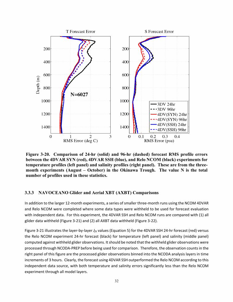
32
Figure 3-20. Comparison of 24-hr (solid) and 96-hr (dashed) forecast RMS profile errors between the 4DVAR SYN (red), 4DVAR SSH (blue), and Relo NCOM (black) experiments for temperature profiles (left panel) and salinity profiles (right panel). These are from the three-month experiments (August – October) in the Okinawa Trough. The value N is the total number of profiles used in these statistics.
3.3.3 NAVOCEANO Glider and Aerial XBT (AXBT) Comparisons
In addition to the larger 12‐month experiments, a series of smaller three‐month runs using the NCOM 4DVAR
and Relo NCOM were completed where some data types were withheld to be used for forecast evaluation
with independent data. For this experiment, the 4DVAR SSH and Relo NCOM runs are compared with (1) all
glider data withheld (Figure 3‐21) and (2) all AXBT data withheld (Figure 3‐22).
Figure 3‐21 illustrates the layer‐by‐layer Jfit values (Equation 5) for the 4DVAR SSH 24‐hr forecast (red) versus
the Relo NCOM experiment 24‐hr forecast (black) for temperature (left panel) and salinity (middle panel)
computed against withheld glider observations. It should be noted that the withheld glider observations were
processed through NCODA‐PREP before being used for comparison. Therefore, the observation counts in the
right panel of this figure are the processed glider observations binned into the NCODA analysis layers in time
increments of 3 hours. Clearly, the forecast using 4DVAR SSH outperformed the Relo NCOM according to this
independent data source, with both temperature and salinity errors significantly less than the Relo NCOM
experiment through all model layers.
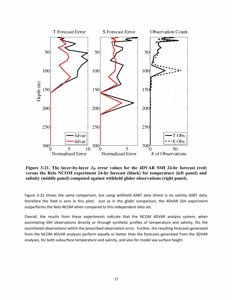
33
Figure 3-21. The layer-by-layer Jfit error values for the 4DVAR SSH 24-hr forecast (red) versus the Relo NCOM experiment 24-hr forecast (black) for temperature (left panel) and salinity (middle panel) computed against withheld glider observations (right panel).
Figure 3‐22 shows the same comparison, but using withheld AXBT data (there is no salinity AXBT data,
therefore the field is zero in this plot). Just as in the glider comparison, the 4DVAR SSH experiment
outperforms the Relo NCOM when compared to this independent data set.
Overall, the results from these experiments indicate that the NCOM 4DVAR analysis system, when
assimilating SSH observations directly or through synthetic profiles of temperature and salinity, fits the
assimilated observations within the prescribed observation error. Further, the resulting forecasts generated
from the NCOM 4DVAR analyses perform equally or better than the forecasts generated from the 3DVAR
analyses, for both subsurface temperature and salinity, and also for model sea surface height.
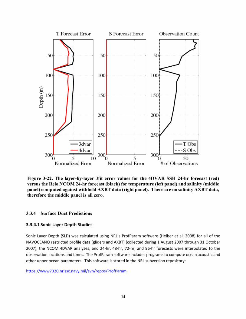
34
Figure 3-22. The layer-by-layer Jfit error values for the 4DVAR SSH 24-hr forecast (red) versus the Relo NCOM 24-hr forecast (black) for temperature (left panel) and salinity (middle panel) computed against withheld AXBT data (right panel). There are no salinity AXBT data, therefore the middle panel is all zero.
3.3.4 Surface Duct Predictions
3.3.4.1 Sonic Layer Depth Studies
Sonic Layer Depth (SLD) was calculated using NRL’s ProfParam software (Helber et al, 2008) for all of the
NAVOCEANO restricted profile data (gliders and AXBT) (collected during 1 August 2007 through 31 October
2007), the NCOM 4DVAR analyses, and 24‐hr, 48‐hr, 72‐hr, and 96‐hr forecasts were interpolated to the
observation locations and times. The ProfParam software includes programs to compute ocean acoustic and
other upper ocean parameters. This software is stored in the NRL subversion repository:
https://www7320.nrlssc.navy.mil/svn/repos/ProfParam
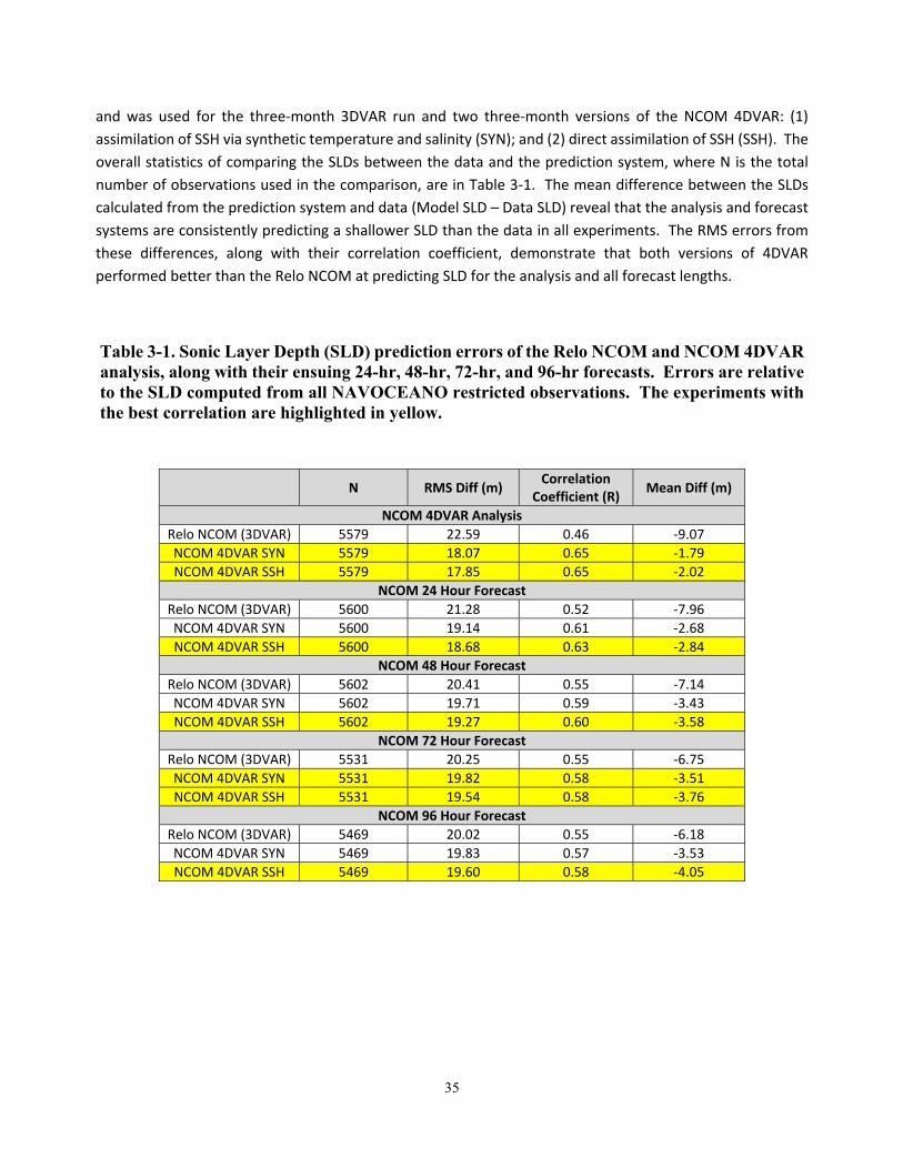
35
and was used for the three‐month 3DVAR run and two three‐month versions of the NCOM 4DVAR: (1)
assimilation of SSH via synthetic temperature and salinity (SYN); and (2) direct assimilation of SSH (SSH). The
overall statistics of comparing the SLDs between the data and the prediction system, where N is the total
number of observations used in the comparison, are in Table 3‐1. The mean difference between the SLDs
calculated from the prediction system and data (Model SLD – Data SLD) reveal that the analysis and forecast
systems are consistently predicting a shallower SLD than the data in all experiments. The RMS errors from
these differences, along with their correlation coefficient, demonstrate that both versions of 4DVAR
performed better than the Relo NCOM at predicting SLD for the analysis and all forecast lengths.
Table 3-1. Sonic Layer Depth (SLD) prediction errors of the Relo NCOM and NCOM 4DVAR analysis, along with their ensuing 24-hr, 48-hr, 72-hr, and 96-hr forecasts. Errors are relative to the SLD computed from all NAVOCEANO restricted observations. The experiments with the best correlation are highlighted in yellow.
N RMS Diff (m) Correlation
Coefficient (R) Mean Diff (m)
NCOM 4DVAR Analysis
Relo NCOM (3DVAR) 5579 22.59 0.46 ‐9.07
NCOM 4DVAR SYN 5579 18.07 0.65 ‐1.79
NCOM 4DVAR SSH 5579 17.85 0.65 ‐2.02
NCOM 24 Hour Forecast
Relo NCOM (3DVAR) 5600 21.28 0.52 ‐7.96
NCOM 4DVAR SYN 5600 19.14 0.61 ‐2.68
NCOM 4DVAR SSH 5600 18.68 0.63 ‐2.84
NCOM 48 Hour Forecast
Relo NCOM (3DVAR) 5602 20.41 0.55 ‐7.14
NCOM 4DVAR SYN 5602 19.71 0.59 ‐3.43
NCOM 4DVAR SSH 5602 19.27 0.60 ‐3.58
NCOM 72 Hour Forecast
Relo NCOM (3DVAR) 5531 20.25 0.55 ‐6.75
NCOM 4DVAR SYN 5531 19.82 0.58 ‐3.51
NCOM 4DVAR SSH 5531 19.54 0.58 ‐3.76
NCOM 96 Hour Forecast
Relo NCOM (3DVAR) 5469 20.02 0.55 ‐6.18
NCOM 4DVAR SYN 5469 19.83 0.57 ‐3.53
NCOM 4DVAR SSH 5469 19.60 0.58 ‐4.05
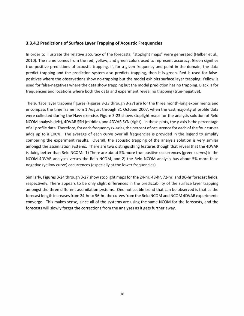
36
3.3.4.2 Predictions of Surface Layer Trapping of Acoustic Frequencies
In order to illustrate the relative accuracy of the forecasts, “stoplight maps” were generated (Helber et al.,
2010). The name comes from the red, yellow, and green colors used to represent accuracy. Green signifies
true‐positive predictions of acoustic trapping. If, for a given frequency and point in the domain, the data
predict trapping and the prediction system also predicts trapping, then it is green. Red is used for false‐
positives where the observations show no‐trapping but the model exhibits surface layer trapping. Yellow is
used for false‐negatives where the data show trapping but the model prediction has no trapping. Black is for
frequencies and locations where both the data and experiment reveal no trapping (true‐negative). The surface layer trapping figures (Figures 3‐23 through 3‐27) are for the three month‐long experiments and
encompass the time frame from 1 August through 31 October 2007, when the vast majority of profile data
were collected during the Navy exercise. Figure 3‐23 shows stoplight maps for the analysis solution of Relo
NCOM analysis (left), 4DVAR SSH (middle), and 4DVAR SYN (right). In these plots, the y‐axis is the percentage
of all profile data. Therefore, for each frequency (x‐axis), the percent of occurrence for each of the four curves
adds up to a 100%. The average of each curve over all frequencies is provided in the legend to simplify
comparing the experiment results. Overall, the acoustic trapping of the analysis solution is very similar
amongst the assimilation systems. There are two distinguishing features though that reveal that the 4DVAR
is doing better than Relo NCOM: 1) There are about 5% more true positive occurrences (green curves) in the
NCOM 4DVAR analyses verses the Relo NCOM, and 2) the Relo NCOM analysis has about 5% more false
negative (yellow curve) occurrences (especially at the lower frequencies).
Similarly, Figures 3‐24 through 3‐27 show stoplight maps for the 24‐hr, 48‐hr, 72‐hr, and 96‐hr forecast fields,
respectively. There appears to be only slight differences in the predictability of the surface layer trapping
amongst the three different assimilation systems. One noticeable trend that can be observed is that as the
forecast length increases from 24‐hr to 96‐hr, the curves from the Relo NCOM and NCOM 4DVAR experiments
converge. This makes sense, since all of the systems are using the same NCOM for the forecasts, and the
forecasts will slowly forget the corrections from the analyses as it gets further away.
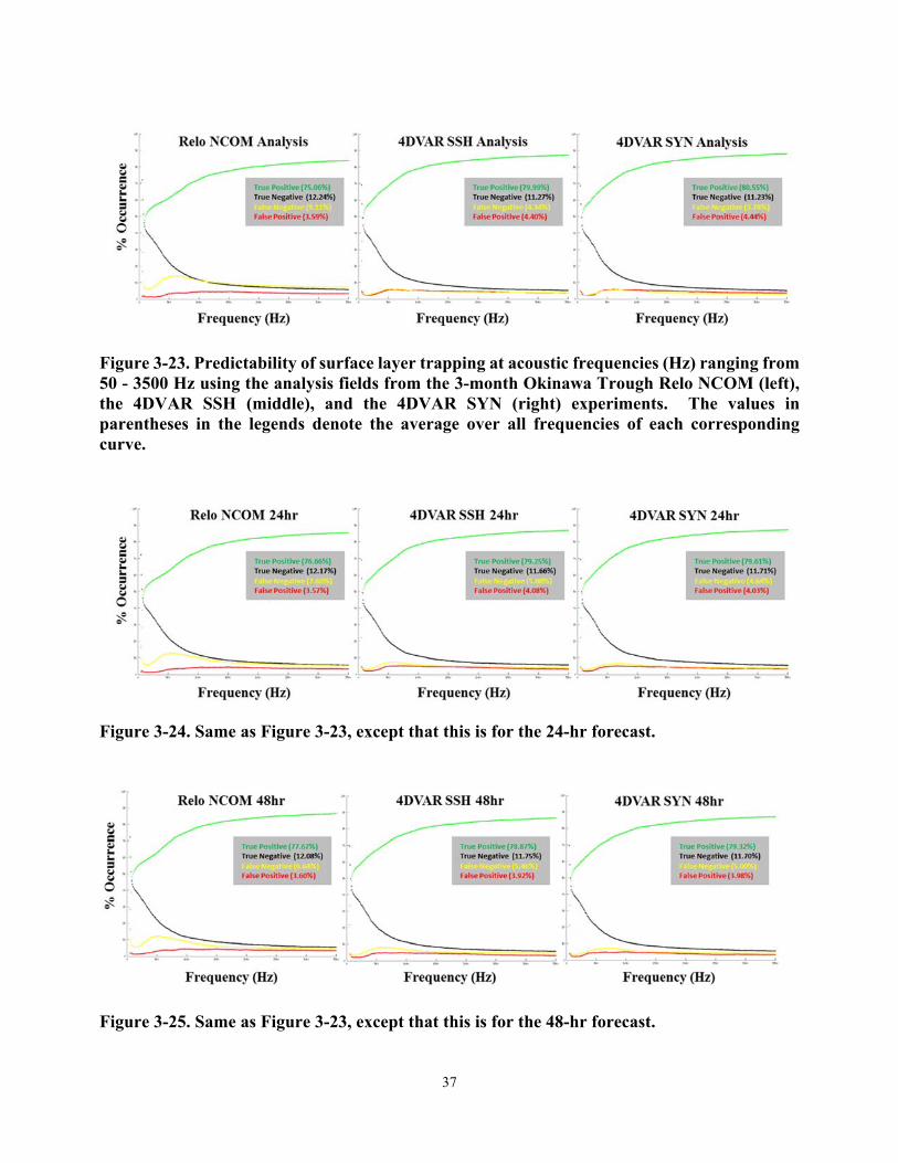
37
Figure 3-23. Predictability of surface layer trapping at acoustic frequencies (Hz) ranging from 50 - 3500 Hz using the analysis fields from the 3-month Okinawa Trough Relo NCOM (left), the 4DVAR SSH (middle), and the 4DVAR SYN (right) experiments. The values in parentheses in the legends denote the average over all frequencies of each corresponding curve.
Figure 3-24. Same as Figure 3-23, except that this is for the 24-hr forecast.
Figure 3-25. Same as Figure 3-23, except that this is for the 48-hr forecast.
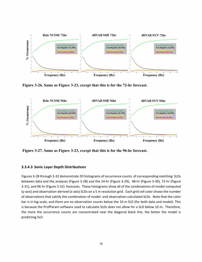
38
Figure 3-26. Same as Figure 3-23, except that this is for the 72-hr forecast.
Figure 3-27. Same as Figure 3-23, except that this is for the 96-hr forecast.
3.3.4.3 Sonic Layer Depth Distributions
Figures 3‐28 through 3‐32 demonstrate 2D histograms of occurrence counts of corresponding matching SLDs
between data and the analyses (Figure 3‐28) and the 24‐hr (Figure 3‐29), 48‐hr (Figure 3‐30), 72‐hr (Figure
3‐31), and 96‐hr (Figure 3‐32) forecasts. These histograms show all of the combinations of model‐computed
(y‐axis) and observation‐derived (x‐axis) SLDs on a 5 m resolution grid. Each grid cell color shows the number
of observations that satisfy the combination of model‐ and observation‐calculated SLDs. Note that the color
bar is in log scale, and there are no observation counts below the 10 m SLD (for both data and model). This
is because the ProfParam software used to calculate SLDs does not allow for a SLD below 10 m. Therefore,
the more the occurrence counts are concentrated near the diagonal black line, the better the model is
predicting SLD.
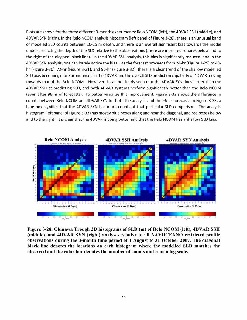
39
Plots are shown for the three different 3‐month experiments: Relo NCOM (left), the 4DVAR SSH (middle), and
4DVAR SYN (right). In the Relo NCOM analysis histogram (left panel of Figure 3‐28), there is an unusual band
of modeled SLD counts between 10‐15 m depth, and there is an overall significant bias towards the model
under‐predicting the depth of the SLD relative to the observations (there are more red squares below and to
the right of the diagonal black line). In the 4DVAR SSH analysis, this bias is significantly reduced; and in the
4DVAR SYN analysis, one can barely notice the bias. As the forecast proceeds from 24‐hr (Figure 3‐29) to 48‐
hr (Figure 3‐30), 72‐hr (Figure 3‐31), and 96‐hr (Figure 3‐32), there is a clear trend of the shallow modelled
SLD bias becoming more pronounced in the 4DVAR and the overall SLD prediction capability of 4DVAR moving
towards that of the Relo NCOM. However, it can be clearly seen that the 4DVAR SYN does better than the
4DVAR SSH at predicting SLD, and both 4DVAR systems perform significantly better than the Relo NCOM
(even after 96‐hr of forecasts). To better visualize this improvement, Figure 3‐33 shows the difference in
counts between Relo NCOM and 4DVAR SYN for both the analysis and the 96‐hr forecast. In Figure 3‐33, a
blue box signifies that the 4DVAR SYN has more counts at that particular SLD comparison. The analysis
histogram (left panel of Figure 3‐33) has mostly blue boxes along and near the diagonal, and red boxes below
and to the right; it is clear that the 4DVAR is doing better and that the Relo NCOM has a shallow SLD bias.
Figure 3-28. Okinawa Trough 2D histograms of SLD (m) of Relo NCOM (left), 4DVAR SSH (middle), and 4DVAR SYN (right) analyses relative to all NAVOCEANO restricted profile observations during the 3-month time period of 1 August to 31 October 2007. The diagonal black line denotes the locations on each histogram where the modelled SLD matches the observed and the color bar denotes the number of counts and is on a log scale.
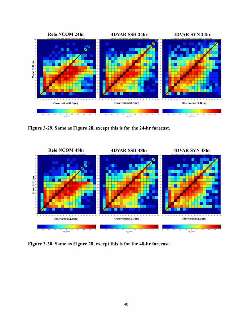
40
Figure 3-29. Same as Figure 28, except this is for the 24-hr forecast.
Figure 3-30. Same as Figure 28, except this is for the 48-hr forecast.
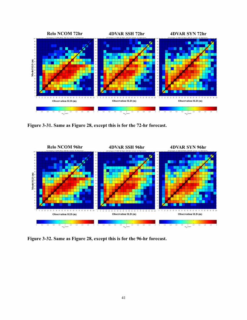
41
Figure 3-31. Same as Figure 28, except this is for the 72-hr forecast.
Figure 3-32. Same as Figure 28, except this is for the 96-hr forecast.
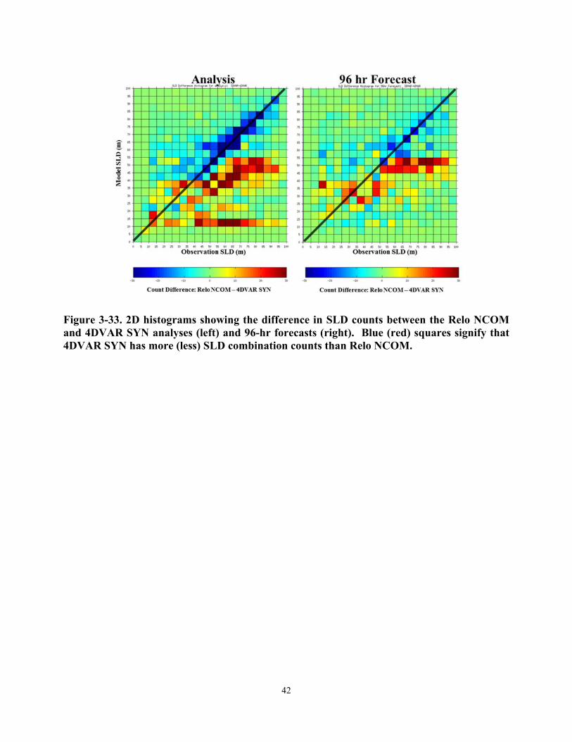
42
Figure 3-33. 2D histograms showing the difference in SLD counts between the Relo NCOM and 4DVAR SYN analyses (left) and 96-hr forecasts (right). Blue (red) squares signify that 4DVAR SYN has more (less) SLD combination counts than Relo NCOM.
43
4.0 RESULTS:OTHERREGIONS
The NCOM 4DVAR system has been validated and verified successfully for a number of field cases. These test
cases evaluated the prediction system’s ability to assimilate hydrographic data from different ocean
domains. The test areas represent regions where significant changeability and enough data existed to
accurately characterize system variability. The prediction system needed to be tested under different
environmental conditions, at different resolutions, and with different flow conditions. It must be capable of
working in myriad locations.
All of the experiments utilized a spherical grid projection and incorporated data from NAVOCEANO’s decoded
data stream that is processed by NCODA‐QC (Cummings, 2011) in near real time (NRT). The NRT quality
control (QC) decisions were used here to select data for assimilation.
4.1 MontereyBay
Due to its complex coastline with steep topography, strong land/sea breeze patterns, and frequent local
upwelling and relaxation events, Monterey Bay, California is a good location to evaluate ocean models
(Shulman et al., 2002). The domain covers 35.6° N to 37.49° N and 121.38° W to 123.2° W (Figure 4‐1). The
NCOM 4DVAR was initialized 1 August 2003 and ran for one month until 1 September 2003. (Ngodock and
Carrier, 2014)
Monterey Bay is part of the larger California Coastal Current System (CCS). Most of the assimilation
experiments that have been completed in Monterey Bay were based on sequential methods such as Multi‐
Variate Optimal Interpolation (MVOI) and ensemble‐based Kalman filters (Chao et al., 2009; Haley et al., 2009;
and Shulman et al., 2009). This test case presents an application of the weak constraint NCOM 4DVAR in
Monterey Bay in a proof‐of‐concept context, using synthetic and real observations. The first objective was to
demonstrate the system’s ability to reduce large discrepancies between the model and the observations,
when the latter were assigned very low errors (Ngodock and Carrier, 2014).
During the summer of 2003, researchers gathered at Monterey Bay Aquarium Research Institute (MBARI) for
a month‐long experiment to study upwelling features in Monterey Bay. Observations were taken using 12
Slocum gliders (CTD and optical properties) and five Spray gliders (CTD), as well as satellites, drifters,
moorings, radars, ship deployed CTDs, and tow‐fish. The glider observations were essential components of
the Autonomous Ocean Sampling Network (AOSN).
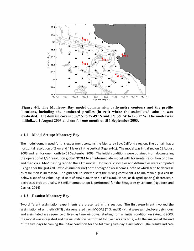
44
Figure 4-1. The Monterey Bay model domain with bathymetry contours and the profile locations, including the numbered profiles (in red) where the assimilated solution was evaluated. The domain covers 35.6° N to 37.49° N and 121.38° W to 123.2° W. The model was initialized 1 August 2003 and ran for one month until 1 September 2003.
4.1.1 Model Set-up: Monterey Bay
The model domain used for this experiment contains the Monterey Bay, California region. The domain has a
horizontal resolution of 2 km and 41 layers in the vertical (Figure 4‐1). The model was initialized on 01 August
2003 and ran for one month to 01 September 2003. The initial conditions were obtained from downscaling
the operational 1/8° resolution global NCOM to an intermediate model with horizontal resolution of 6 km,
and then via a 3‐to‐1 nesting ratio to the 2 km model. Horizontal viscosities and diffusivities were computed
using either the grid‐cell Reynolds number (Re) or the Smagorinsky schemes, both of which tend to decrease
as resolution is increased. The grid‐cell Re scheme sets the mixing coefficient K to maintain a grid cell Re
below a specified value (e.g., if Re = u*dx/K = 30, then K = u*dx/30). Hence, as dx (grid spacing) decreases, K
decreases proportionally. A similar computation is performed for the Smagorinsky scheme. (Ngodock and
Carrier, 2014)
4.1.2 Results: Monterey Bay
Two different assimilation experiments are presented in this section. The first experiment involved the
assimilation of synthetic (SYN) data generated from MODAS (T, S, and SSH) that were sampled every six‐hours
and assimilated in a sequence of five‐day time windows. Starting from an initial condition on 2 August 2003,
the model was integrated and the assimilation performed for five days at a time, with the analysis at the end
of the five days becoming the initial condition for the following five‐day assimilation. The results indicate
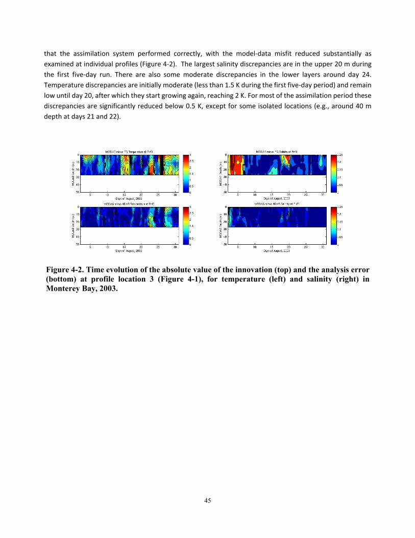
45
that the assimilation system performed correctly, with the model‐data misfit reduced substantially as
examined at individual profiles (Figure 4‐2). The largest salinity discrepancies are in the upper 20 m during
the first five‐day run. There are also some moderate discrepancies in the lower layers around day 24.
Temperature discrepancies are initially moderate (less than 1.5 K during the first five‐day period) and remain
low until day 20, after which they start growing again, reaching 2 K. For most of the assimilation period these
discrepancies are significantly reduced below 0.5 K, except for some isolated locations (e.g., around 40 m
depth at days 21 and 22).
Figure 4-2. Time evolution of the absolute value of the innovation (top) and the analysis error (bottom) at profile location 3 (Figure 4-1), for temperature (left) and salinity (right) in Monterey Bay, 2003.
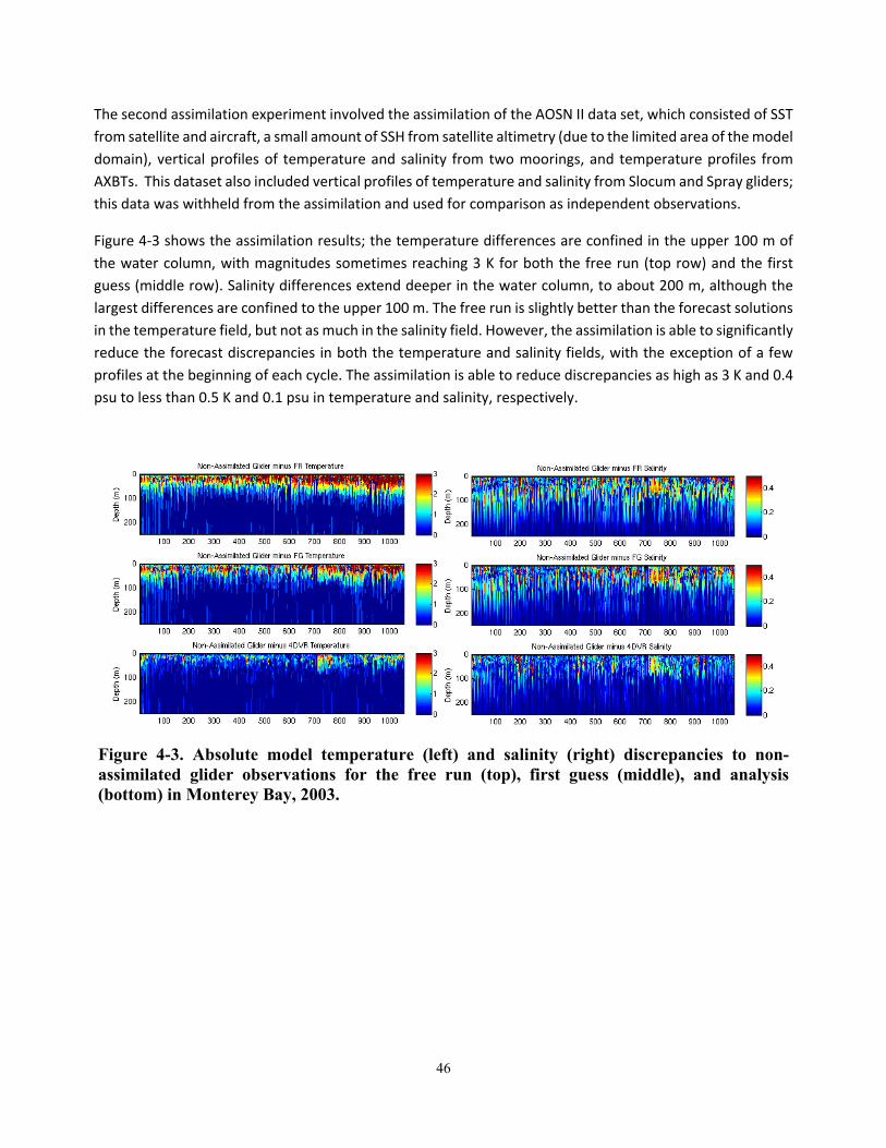
46
The second assimilation experiment involved the assimilation of the AOSN II data set, which consisted of SST
from satellite and aircraft, a small amount of SSH from satellite altimetry (due to the limited area of the model
domain), vertical profiles of temperature and salinity from two moorings, and temperature profiles from
AXBTs. This dataset also included vertical profiles of temperature and salinity from Slocum and Spray gliders;
this data was withheld from the assimilation and used for comparison as independent observations.
Figure 4‐3 shows the assimilation results; the temperature differences are confined in the upper 100 m of
the water column, with magnitudes sometimes reaching 3 K for both the free run (top row) and the first
guess (middle row). Salinity differences extend deeper in the water column, to about 200 m, although the
largest differences are confined to the upper 100 m. The free run is slightly better than the forecast solutions
in the temperature field, but not as much in the salinity field. However, the assimilation is able to significantly
reduce the forecast discrepancies in both the temperature and salinity fields, with the exception of a few
profiles at the beginning of each cycle. The assimilation is able to reduce discrepancies as high as 3 K and 0.4
psu to less than 0.5 K and 0.1 psu in temperature and salinity, respectively.
Figure 4-3. Absolute model temperature (left) and salinity (right) discrepancies to non-assimilated glider observations for the free run (top), first guess (middle), and analysis (bottom) in Monterey Bay, 2003.
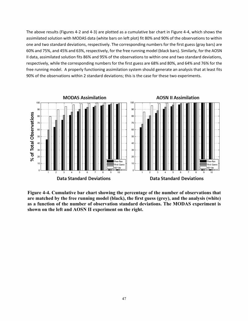
47
The above results (Figures 4‐2 and 4‐3) are plotted as a cumulative bar chart in Figure 4‐4, which shows the
assimilated solution with MODAS data (white bars on left plot) fit 80% and 90% of the observations to within
one and two standard deviations, respectively. The corresponding numbers for the first guess (gray bars) are
60% and 75%, and 45% and 63%, respectively, for the free running model (black bars). Similarly, for the AOSN
II data, assimilated solution fits 86% and 95% of the observations to within one and two standard deviations,
respectively, while the corresponding numbers for the first guess are 68% and 80%, and 64% and 76% for the
free running model. A properly functioning assimilation system should generate an analysis that at least fits
90% of the observations within 2 standard deviations; this is the case for these two experiments.
Figure 4-4. Cumulative bar chart showing the percentage of the number of observations that are matched by the free running model (black), the first guess (grey), and the analysis (white) as a function of the number of observation standard deviations. The MODAS experiment is shown on the left and AOSN II experiment on the right.
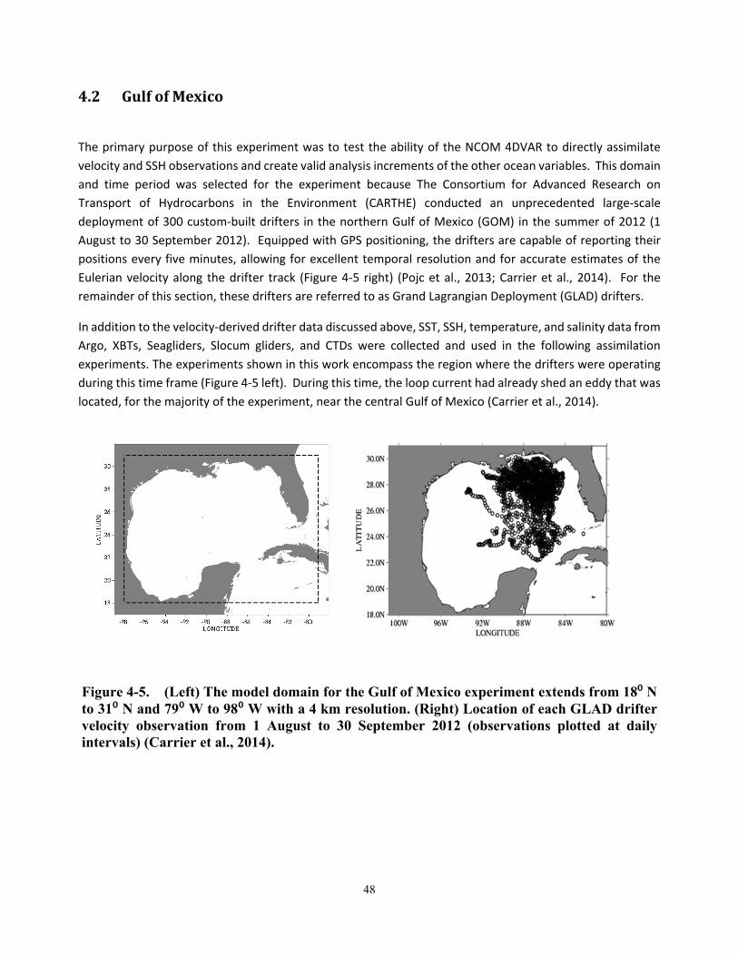
48
4.2 GulfofMexico
The primary purpose of this experiment was to test the ability of the NCOM 4DVAR to directly assimilate
velocity and SSH observations and create valid analysis increments of the other ocean variables. This domain
and time period was selected for the experiment because The Consortium for Advanced Research on
Transport of Hydrocarbons in the Environment (CARTHE) conducted an unprecedented large‐scale
deployment of 300 custom‐built drifters in the northern Gulf of Mexico (GOM) in the summer of 2012 (1
August to 30 September 2012). Equipped with GPS positioning, the drifters are capable of reporting their
positions every five minutes, allowing for excellent temporal resolution and for accurate estimates of the
Eulerian velocity along the drifter track (Figure 4‐5 right) (Pojc et al., 2013; Carrier et al., 2014). For the
remainder of this section, these drifters are referred to as Grand Lagrangian Deployment (GLAD) drifters.
In addition to the velocity‐derived drifter data discussed above, SST, SSH, temperature, and salinity data from
Argo, XBTs, Seagliders, Slocum gliders, and CTDs were collected and used in the following assimilation
experiments. The experiments shown in this work encompass the region where the drifters were operating
during this time frame (Figure 4‐5 left). During this time, the loop current had already shed an eddy that was
located, for the majority of the experiment, near the central Gulf of Mexico (Carrier et al., 2014).
Figure 4-5. (Left) The model domain for the Gulf of Mexico experiment extends from 18⁰ N to 31⁰ N and 79⁰ W to 98⁰ W with a 4 km resolution. (Right) Location of each GLAD drifter velocity observation from 1 August to 30 September 2012 (observations plotted at daily intervals) (Carrier et al., 2014).
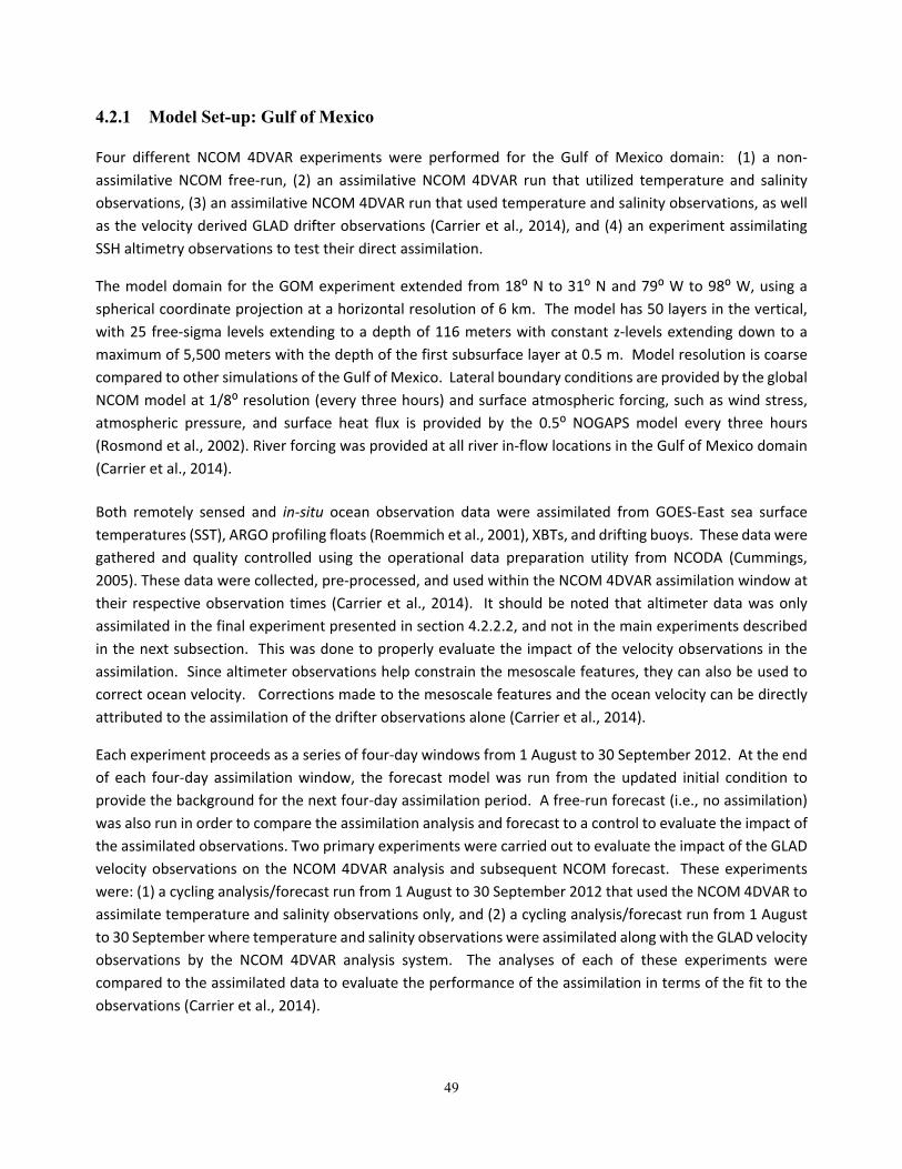
49
4.2.1 Model Set-up: Gulf of Mexico
Four different NCOM 4DVAR experiments were performed for the Gulf of Mexico domain: (1) a non‐
assimilative NCOM free‐run, (2) an assimilative NCOM 4DVAR run that utilized temperature and salinity
observations, (3) an assimilative NCOM 4DVAR run that used temperature and salinity observations, as well
as the velocity derived GLAD drifter observations (Carrier et al., 2014), and (4) an experiment assimilating
SSH altimetry observations to test their direct assimilation.
The model domain for the GOM experiment extended from 18⁰ N to 31⁰ N and 79⁰ W to 98⁰ W, using a
spherical coordinate projection at a horizontal resolution of 6 km. The model has 50 layers in the vertical,
with 25 free‐sigma levels extending to a depth of 116 meters with constant z‐levels extending down to a
maximum of 5,500 meters with the depth of the first subsurface layer at 0.5 m. Model resolution is coarse
compared to other simulations of the Gulf of Mexico. Lateral boundary conditions are provided by the global
NCOM model at 1/8⁰ resolution (every three hours) and surface atmospheric forcing, such as wind stress,
atmospheric pressure, and surface heat flux is provided by the 0.5⁰ NOGAPS model every three hours
(Rosmond et al., 2002). River forcing was provided at all river in‐flow locations in the Gulf of Mexico domain
(Carrier et al., 2014).
Both remotely sensed and in‐situ ocean observation data were assimilated from GOES‐East sea surface
temperatures (SST), ARGO profiling floats (Roemmich et al., 2001), XBTs, and drifting buoys. These data were
gathered and quality controlled using the operational data preparation utility from NCODA (Cummings,
2005). These data were collected, pre‐processed, and used within the NCOM 4DVAR assimilation window at
their respective observation times (Carrier et al., 2014). It should be noted that altimeter data was only
assimilated in the final experiment presented in section 4.2.2.2, and not in the main experiments described
in the next subsection. This was done to properly evaluate the impact of the velocity observations in the
assimilation. Since altimeter observations help constrain the mesoscale features, they can also be used to
correct ocean velocity. Corrections made to the mesoscale features and the ocean velocity can be directly
attributed to the assimilation of the drifter observations alone (Carrier et al., 2014).
Each experiment proceeds as a series of four‐day windows from 1 August to 30 September 2012. At the end
of each four‐day assimilation window, the forecast model was run from the updated initial condition to
provide the background for the next four‐day assimilation period. A free‐run forecast (i.e., no assimilation)
was also run in order to compare the assimilation analysis and forecast to a control to evaluate the impact of
the assimilated observations. Two primary experiments were carried out to evaluate the impact of the GLAD
velocity observations on the NCOM 4DVAR analysis and subsequent NCOM forecast. These experiments
were: (1) a cycling analysis/forecast run from 1 August to 30 September 2012 that used the NCOM 4DVAR to
assimilate temperature and salinity observations only, and (2) a cycling analysis/forecast run from 1 August
to 30 September where temperature and salinity observations were assimilated along with the GLAD velocity
observations by the NCOM 4DVAR analysis system. The analyses of each of these experiments were
compared to the assimilated data to evaluate the performance of the assimilation in terms of the fit to the
observations (Carrier et al., 2014).
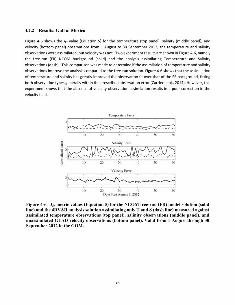
50
4.2.2 Results: Gulf of Mexico
Figure 4‐6 shows the Jfit value (Equation 5) for the temperature (top panel), salinity (middle panel), and
velocity (bottom panel) observations from 1 August to 30 September 2012; the temperature and salinity
observations were assimilated, but velocity was not. Two experiment results are shown in Figure 4‐6, namely
the free‐run (FR) NCOM background (solid) and the analysis assimilating Temperature and Salinity
observations (dash). This comparison was made to determine if the assimilation of temperature and salinity
observations improve the analysis compared to the free‐run solution. Figure 4‐6 shows that the assimilation
of temperature and salinity has greatly improved the observation fit over that of the FR background, fitting
both observation types generally within the prescribed observation error (Carrier et al., 2014). However, this
experiment shows that the absence of velocity observation assimilation results in a poor correction in the
velocity field.
Figure 4-6. Jfit metric values (Equation 5) for the NCOM free-run (FR) model solution (solid line) and the 4DVAR analysis solution assimilating only T and S (dash line) measured against assimilated temperature observations (top panel), salinity observations (middle panel), and unassimilated GLAD velocity observations (bottom panel). Valid from 1 August through 30 September 2012 in the GOM.
51
Figure 4‐7 shows the Jfit value of the analysis assimilating just temperature and observations (solid) and the
analysis assimilating all observations (dash). The solid lines in Figure 4‐7 is the same as the dashed lines in
Figure 4‐6. The only difference in the analysis solutions created by these two experiments is that one of them
also includes the assimilation of the GLAD velocity data (dash). Therefore, Figure 4‐7 shows that by including
additional GLAD velocity data in the assimilation, the accuracy of the temperature and salinity analysis
doesn’t change that much, but the analysis of velocity is drastically improved.
Figure 4-7. Jfit metric values for the analysis solution assimilating just temperature and salinity (solid line) and the analysis solution that assimilated all data (dash line) measured against assimilated temperature (top panel), salinity (middle panel), and GLAD velocity observations (bottom panel). Valid from 1 August through 30 September 2012.
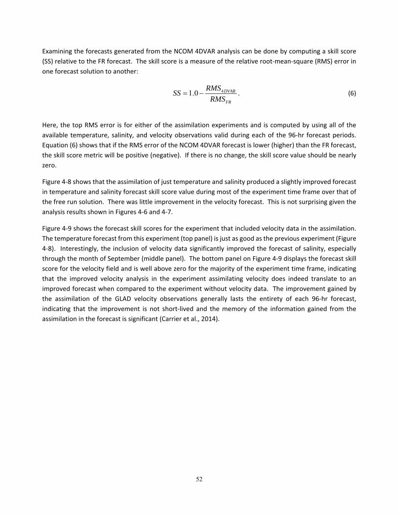
52
Examining the forecasts generated from the NCOM 4DVAR analysis can be done by computing a skill score
(SS) relative to the FR forecast. The skill score is a measure of the relative root‐mean‐square (RMS) error in
one forecast solution to another:
41.0 DVAR
FR
RMSSS
RMS . (6)
Here, the top RMS error is for either of the assimilation experiments and is computed by using all of the
available temperature, salinity, and velocity observations valid during each of the 96‐hr forecast periods.
Equation (6) shows that if the RMS error of the NCOM 4DVAR forecast is lower (higher) than the FR forecast,
the skill score metric will be positive (negative). If there is no change, the skill score value should be nearly
zero.
Figure 4‐8 shows that the assimilation of just temperature and salinity produced a slightly improved forecast
in temperature and salinity forecast skill score value during most of the experiment time frame over that of
the free run solution. There was little improvement in the velocity forecast. This is not surprising given the
analysis results shown in Figures 4‐6 and 4‐7.
Figure 4‐9 shows the forecast skill scores for the experiment that included velocity data in the assimilation.
The temperature forecast from this experiment (top panel) is just as good as the previous experiment (Figure
4‐8). Interestingly, the inclusion of velocity data significantly improved the forecast of salinity, especially
through the month of September (middle panel). The bottom panel on Figure 4‐9 displays the forecast skill
score for the velocity field and is well above zero for the majority of the experiment time frame, indicating
that the improved velocity analysis in the experiment assimilating velocity does indeed translate to an
improved forecast when compared to the experiment without velocity data. The improvement gained by
the assimilation of the GLAD velocity observations generally lasts the entirety of each 96‐hr forecast,
indicating that the improvement is not short‐lived and the memory of the information gained from the
assimilation in the forecast is significant (Carrier et al., 2014).
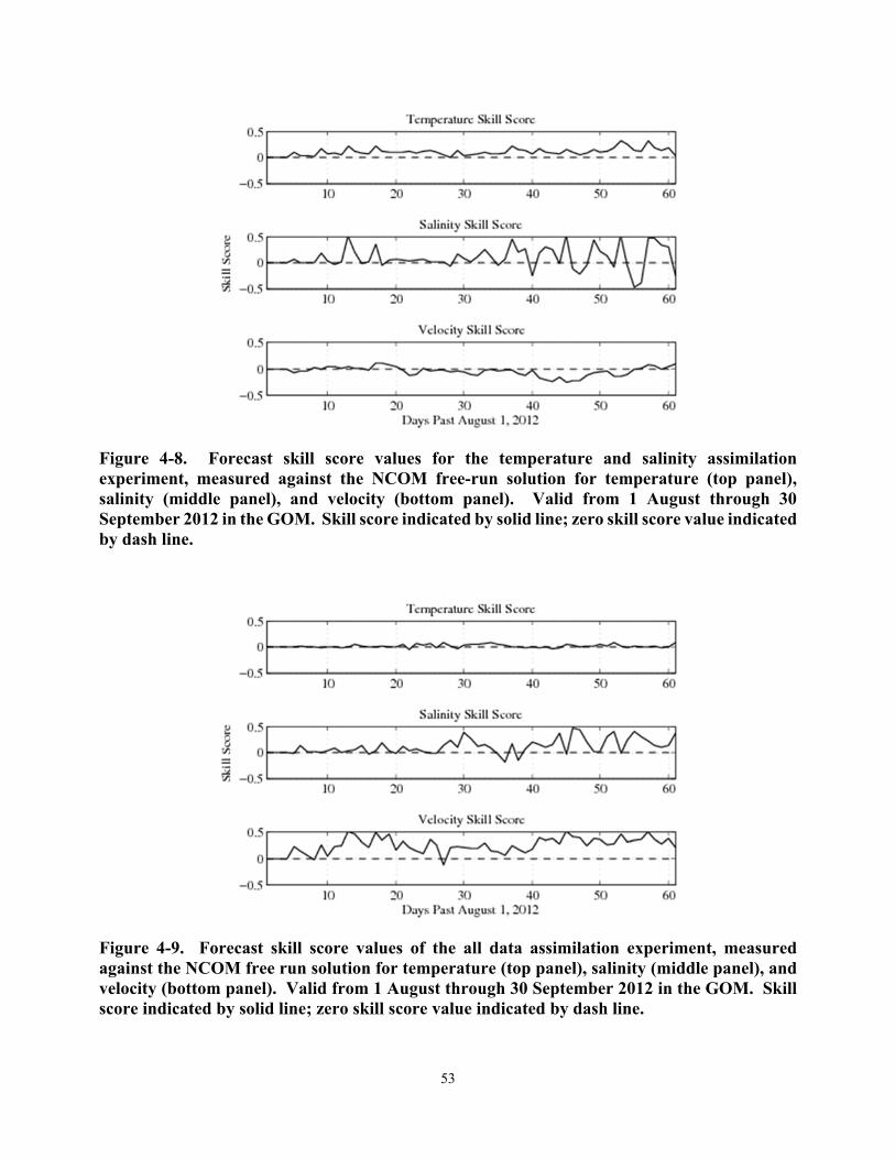
53
Figure 4-8. Forecast skill score values for the temperature and salinity assimilation experiment, measured against the NCOM free-run solution for temperature (top panel), salinity (middle panel), and velocity (bottom panel). Valid from 1 August through 30 September 2012 in the GOM. Skill score indicated by solid line; zero skill score value indicated by dash line.
Figure 4-9. Forecast skill score values of the all data assimilation experiment, measured against the NCOM free run solution for temperature (top panel), salinity (middle panel), and velocity (bottom panel). Valid from 1 August through 30 September 2012 in the GOM. Skill score indicated by solid line; zero skill score value indicated by dash line.
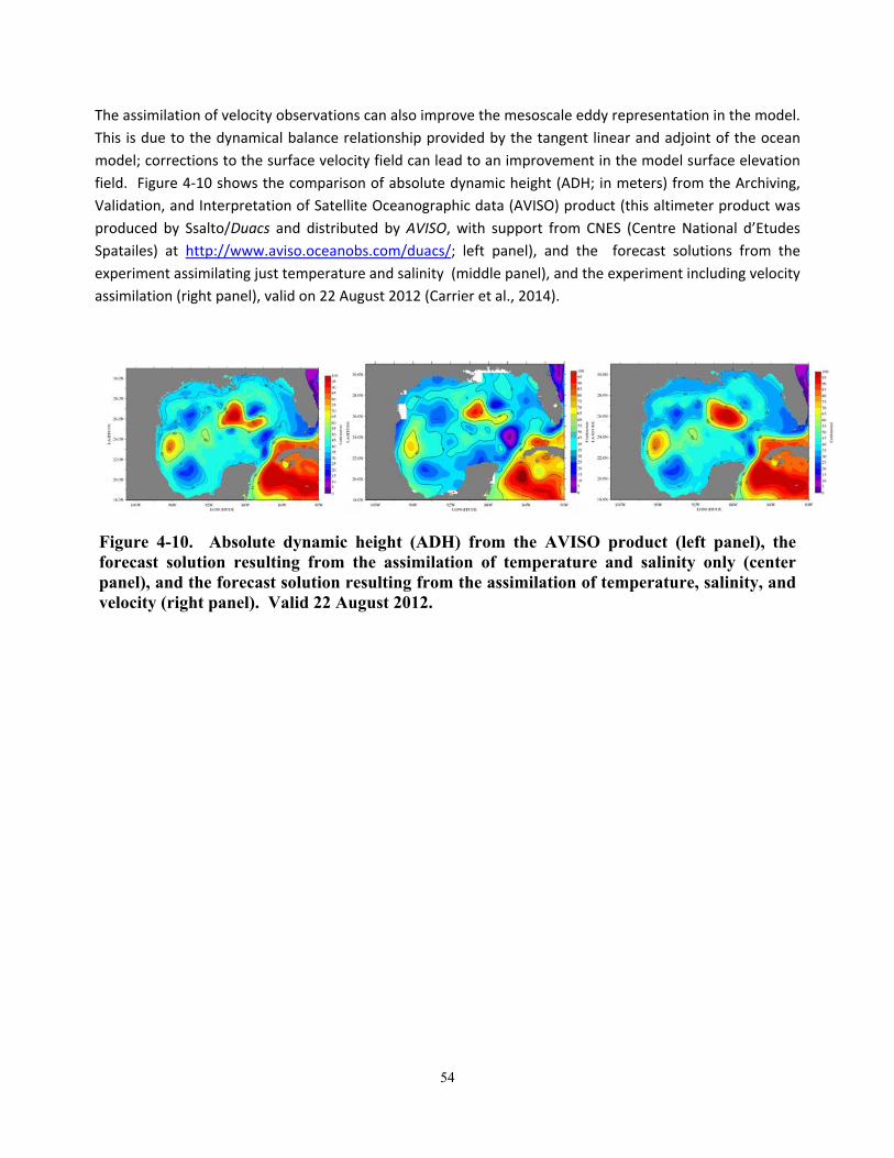
54
The assimilation of velocity observations can also improve the mesoscale eddy representation in the model.
This is due to the dynamical balance relationship provided by the tangent linear and adjoint of the ocean
model; corrections to the surface velocity field can lead to an improvement in the model surface elevation
field. Figure 4‐10 shows the comparison of absolute dynamic height (ADH; in meters) from the Archiving,
Validation, and Interpretation of Satellite Oceanographic data (AVISO) product (this altimeter product was
produced by Ssalto/Duacs and distributed by AVISO, with support from CNES (Centre National d’Etudes
Spatailes) at http://www.aviso.oceanobs.com/duacs/; left panel), and the forecast solutions from the
experiment assimilating just temperature and salinity (middle panel), and the experiment including velocity
assimilation (right panel), valid on 22 August 2012 (Carrier et al., 2014).
Figure 4-10. Absolute dynamic height (ADH) from the AVISO product (left panel), the forecast solution resulting from the assimilation of temperature and salinity only (center panel), and the forecast solution resulting from the assimilation of temperature, salinity, and velocity (right panel). Valid 22 August 2012.
55
The NCOM 4DVAR is able to fit the observations not only in the analysis step, but also in the subsequent
forecasts. By comparing the assimilation results in terms of the analysis fit to the observations, as well as the
subsequent forecast fit to future observations between an experiment with no velocity assimilation (T and S)
and an experiment with velocity assimilation (ALL), we have been able to conclude that assimilating the
surface velocity observations leads to a substantial improvement in not only the analysis fit, but also in the
forecast. The assimilation of velocity observations also led to an improved salinity forecast (center panel of
Figure 4‐10) and it helped to constrain the surface eddy field in the vicinity of the drifter observations (right
panel of Figure 4‐10) (Carrier et al., 2014).
4.2.2.1 Velocity Assimilation
The velocity observations from Lagrangian drifters deployed in the Gulf of Mexico during the summer 2012
GLAD experiment were assimilated into the NCOM 4DVAR analysis system to examine their impact on
Lagrangian predictability. Velocities derived from drifter trajectories, as well as satellite and in situ
observations were assimilated. Lagrangian forecast skill is assessed using separation distance and angular
differences between simulated and observed trajectory positions. Figure 4‐11 shows that assimilating drifter
velocities substantially improves the model forecast shape and position of a Loop Current ring. These gains
in mesoscale Eulerian forecast skill also improve Lagrangian forecasts, reducing the growth rate of separation
distances between observed and simulated drifters by approximately 7.3 km day‐1 on average, when
compared with forecasts that assimilate only temperature and salinity observations. Trajectory angular
differences are also reduced.
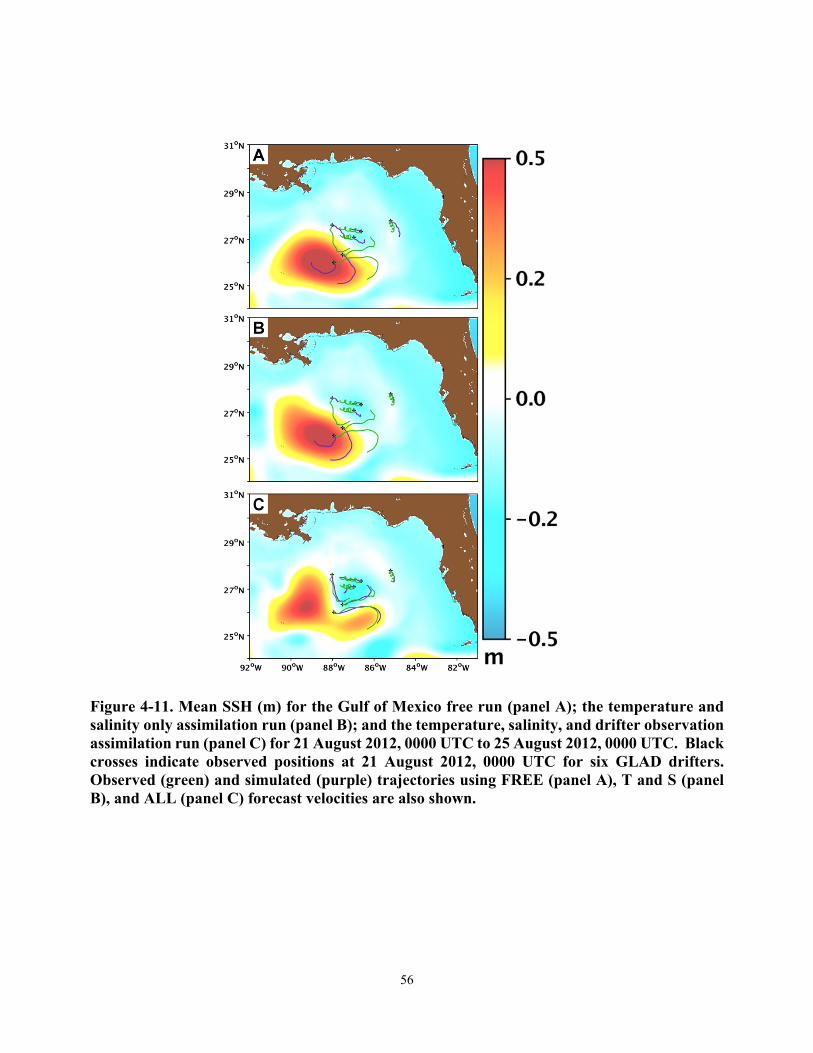
56
Figure 4-11. Mean SSH (m) for the Gulf of Mexico free run (panel A); the temperature and salinity only assimilation run (panel B); and the temperature, salinity, and drifter observation assimilation run (panel C) for 21 August 2012, 0000 UTC to 25 August 2012, 0000 UTC. Black crosses indicate observed positions at 21 August 2012, 0000 UTC for six GLAD drifters. Observed (green) and simulated (purple) trajectories using FREE (panel A), T and S (panel B), and ALL (panel C) forecast velocities are also shown.
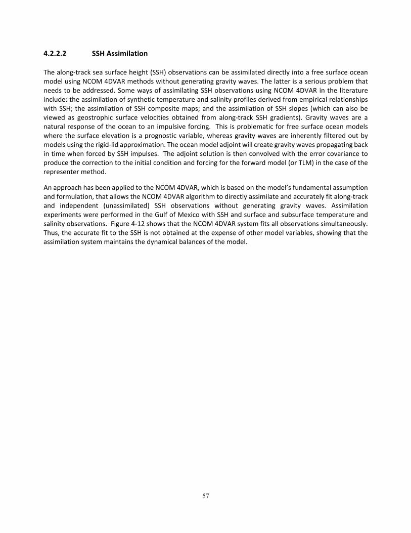
57
4.2.2.2 SSH Assimilation
The along‐track sea surface height (SSH) observations can be assimilated directly into a free surface ocean model using NCOM 4DVAR methods without generating gravity waves. The latter is a serious problem that needs to be addressed. Some ways of assimilating SSH observations using NCOM 4DVAR in the literature include: the assimilation of synthetic temperature and salinity profiles derived from empirical relationships with SSH; the assimilation of SSH composite maps; and the assimilation of SSH slopes (which can also be viewed as geostrophic surface velocities obtained from along‐track SSH gradients). Gravity waves are a natural response of the ocean to an impulsive forcing. This is problematic for free surface ocean models where the surface elevation is a prognostic variable, whereas gravity waves are inherently filtered out by models using the rigid‐lid approximation. The ocean model adjoint will create gravity waves propagating back in time when forced by SSH impulses. The adjoint solution is then convolved with the error covariance to produce the correction to the initial condition and forcing for the forward model (or TLM) in the case of the representer method.
An approach has been applied to the NCOM 4DVAR, which is based on the model’s fundamental assumption and formulation, that allows the NCOM 4DVAR algorithm to directly assimilate and accurately fit along‐track and independent (unassimilated) SSH observations without generating gravity waves. Assimilation experiments were performed in the Gulf of Mexico with SSH and surface and subsurface temperature and salinity observations. Figure 4‐12 shows that the NCOM 4DVAR system fits all observations simultaneously. Thus, the accurate fit to the SSH is not obtained at the expense of other model variables, showing that the assimilation system maintains the dynamical balances of the model.
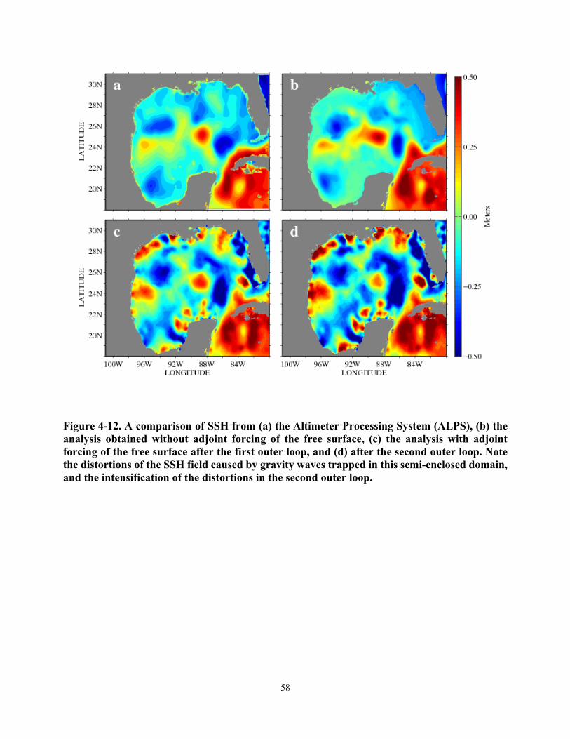
58
Figure 4-12. A comparison of SSH from (a) the Altimeter Processing System (ALPS), (b) the analysis obtained without adjoint forcing of the free surface, (c) the analysis with adjoint forcing of the free surface after the first outer loop, and (d) after the second outer loop. Note the distortions of the SSH field caused by gravity waves trapped in this semi-enclosed domain, and the intensification of the distortions in the second outer loop.
59
4.3 OtherLocationsUsingNCOM4DVAR
The purpose of validating NCOM 4DVAR in other locations is to demonstrate its flexibility and portability in
multiple regions with different hydrodynamic environments, using different resolutions, different forcings,
etc. The model has been tested in the Pacific Rim of Hawaii (RIMPAC), the Middle Atlantic Bight (Mid
Atlantic Bight or MAB), Southern California, and the Kuroshio Extension (Table 4‐1).
Table 4-1. Other geographical locations using NCOM 4DVAR. All data are from the NAVOCEANO Operational Data Stream; other data sources are specified.
LOCATION DATE OBSERVATIONAL DATA LATTITUDE/LONGITUDE GRID RIMPAC (RIMPAC 08)
2008 SST, SSH, T/S (ARGO, XBT), 4 Seagliders, 4 Slocum gliders, CTDs
18°N to 24°N and 162°W to 154°W ~3 km horizontal, 277 x 223 grid
Mid Atlantic Bight 2011 Trident Warrior Exercise 39.5⁰N to 42⁰N and 69.5⁰W to 74.5⁰W 500 m horizontal
Southern California 2013 29⁰N to 44⁰N and 114⁰W to 129⁰W 3 km horizontal
Kuroshio Extension 2010 31.1°N to 38.1°N and 137.1°E to 145.1° E
3 km horizontal, 50 vertical
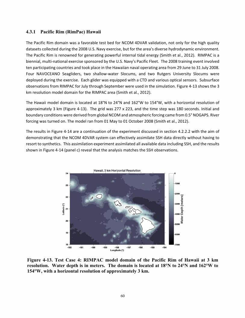
60
4.3.1 Pacific Rim (RimPac) Hawaii
The Pacific Rim domain was a favorable test bed for NCOM 4DVAR validation, not only for the high quality
datasets collected during the 2008 U.S. Navy exercise, but for the area’s diverse hydrodynamic environment.
The Pacific Rim is renowned for generating powerful internal tidal energy (Smith et al., 2012). RIMPAC is a
biennial, multi‐national exercise sponsored by the U.S. Navy’s Pacific Fleet. The 2008 training event involved
ten participating countries and took place in the Hawaiian naval operating area from 29 June to 31 July 2008.
Four NAVOCEANO Seagliders, two shallow‐water Slocums, and two Rutgers University Slocums were
deployed during the exercise. Each glider was equipped with a CTD and various optical sensors. Subsurface
observations from RIMPAC for July through September were used in the simulation. Figure 4‐13 shows the 3
km resolution model domain for the RIMPAC area (Smith et al., 2012).
The Hawaii model domain is located at 18°N to 24°N and 162°W to 154°W, with a horizontal resolution of
approximately 3 km (Figure 4‐13). The grid was 277 x 223, and the time step was 180 seconds. Initial and
boundary conditions were derived from global NCOM and atmospheric forcing came from 0.5° NOGAPS. River
forcing was turned on. The model ran from 01 May to 01 October 2008 (Smith et al., 2012).
The results in Figure 4‐14 are a continuation of the experiment discussed in section 4.2.2.2 with the aim of
demonstrating that the NCOM 4DVAR system can effectively assimilate SSH data directly without having to
resort to synthetics. This assimilation experiment assimilated all available data including SSH, and the results
shown in Figure 4‐14 (panel c) reveal that the analysis matches the SSH observations.
Figure 4-13. Test Case 4: RIMPAC model domain of the Pacific Rim of Hawaii at 3 km resolution. Water depth is in meters. The domain is located at 18°N to 24°N and 162°W to 154°W, with a horizontal resolution of approximately 3 km.
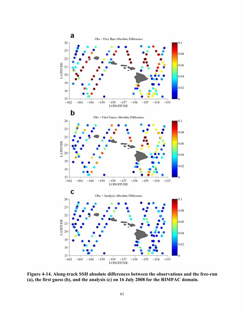
61
Figure 4-14. Along-track SSH absolute differences between the observations and the free-run (a), the first guess (b), and the analysis (c) on 16 July 2008 for the RIMPAC domain.
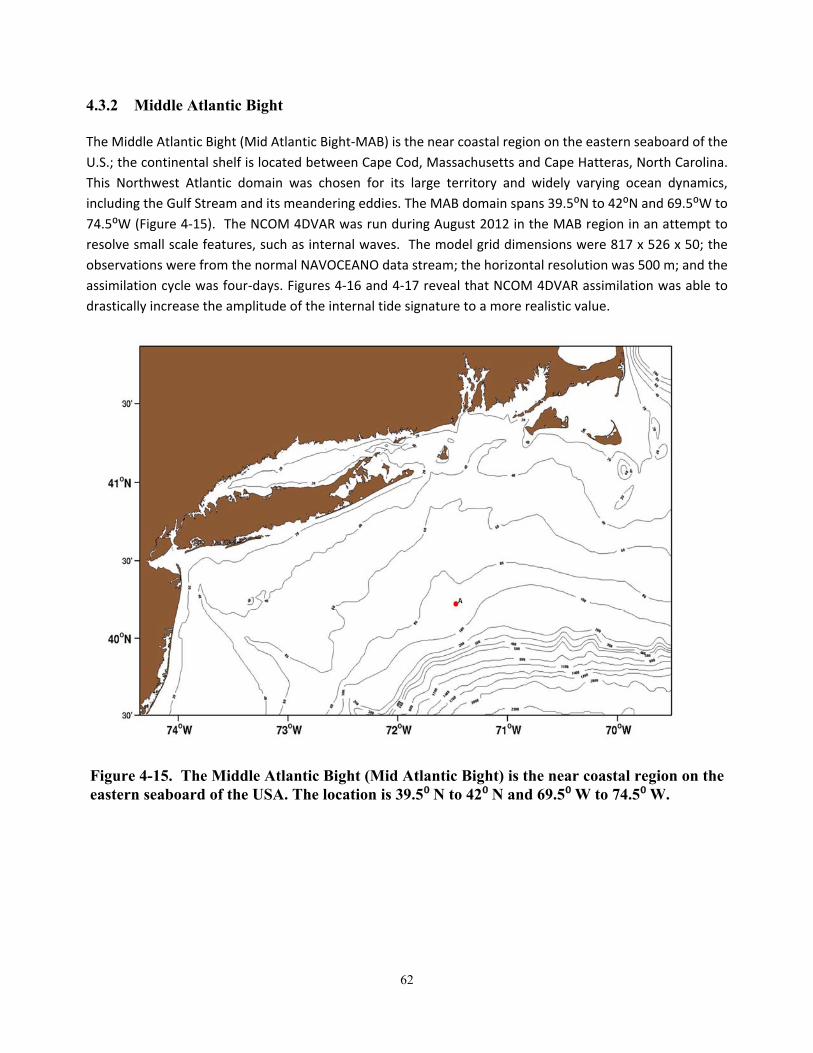
62
4.3.2 Middle Atlantic Bight
The Middle Atlantic Bight (Mid Atlantic Bight‐MAB) is the near coastal region on the eastern seaboard of the
U.S.; the continental shelf is located between Cape Cod, Massachusetts and Cape Hatteras, North Carolina.
This Northwest Atlantic domain was chosen for its large territory and widely varying ocean dynamics,
including the Gulf Stream and its meandering eddies. The MAB domain spans 39.5⁰N to 42⁰N and 69.5⁰W to
74.5⁰W (Figure 4‐15). The NCOM 4DVAR was run during August 2012 in the MAB region in an attempt to
resolve small scale features, such as internal waves. The model grid dimensions were 817 x 526 x 50; the
observations were from the normal NAVOCEANO data stream; the horizontal resolution was 500 m; and the
assimilation cycle was four‐days. Figures 4‐16 and 4‐17 reveal that NCOM 4DVAR assimilation was able to
drastically increase the amplitude of the internal tide signature to a more realistic value.
Figure 4-15. The Middle Atlantic Bight (Mid Atlantic Bight) is the near coastal region on the eastern seaboard of the USA. The location is 39.5⁰N to 42⁰N and 69.5⁰W to 74.5⁰W.
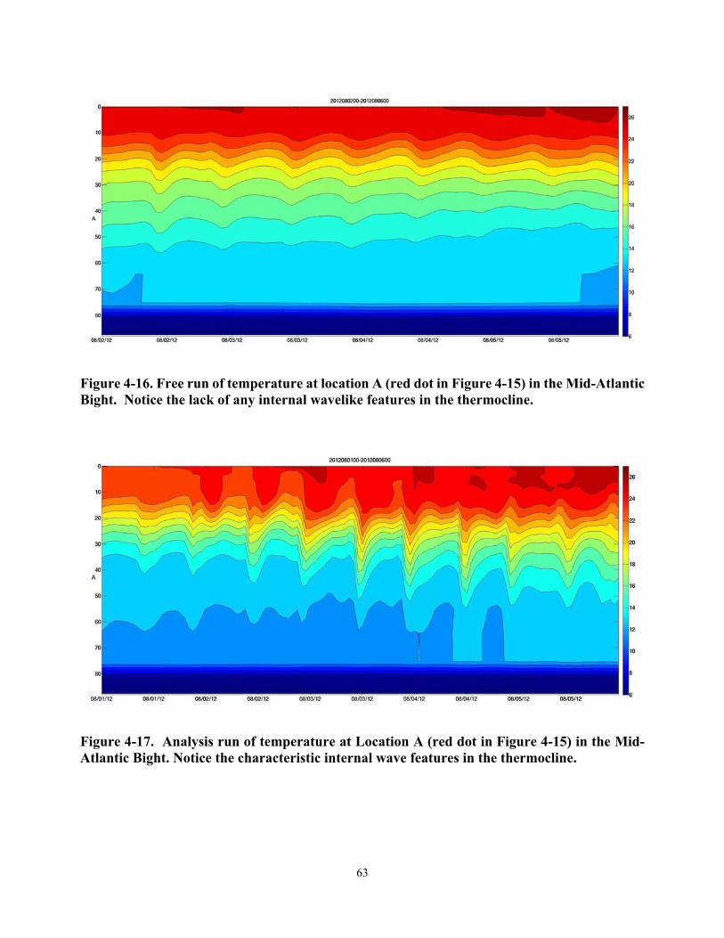
63
Figure 4-16. Free run of temperature at location A (red dot in Figure 4-15) in the Mid-Atlantic Bight. Notice the lack of any internal wavelike features in the thermocline.
Figure 4-17. Analysis run of temperature at Location A (red dot in Figure 4-15) in the Mid-Atlantic Bight. Notice the characteristic internal wave features in the thermocline.
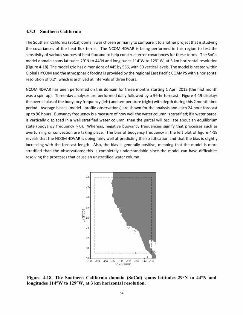
64
4.3.3 Southern California
The Southern California (SoCal) domain was chosen primarily to compare it to another project that is studying
the covariances of the heat flux terms. The NCOM 4DVAR is being performed in this region to test the
sensitivity of various sources of heat flux and to help construct error covariances for these terms. The SoCal
model domain spans latitudes 29°N to 44°N and longitudes 114°W to 129° W, at 3 km horizontal resolution
(Figure 4‐18). The model grid has dimensions of 445 by 556, with 50 vertical levels. The model is nested within
Global HYCOM and the atmospheric forcing is provided by the regional East Pacific COAMPS with a horizontal
resolution of 0.2°, which is archived at intervals of three hours.
NCOM 4DVAR has been performed on this domain for three months starting 1 April 2013 (the first month
was a spin up). Three‐day analyses are performed daily followed by a 96‐hr forecast. Figure 4‐19 displays
the overall bias of the buoyancy frequency (left) and temperature (right) with depth during this 2 month time
period. Average biases (model ‐ profile observations) are shown for the analysis and each 24 hour forecast
up to 96 hours. Buoyancy frequency is a measure of how well the water column is stratified; if a water parcel
is vertically displaced in a well stratified water column, then the parcel will oscillate about an equilibrium
state (buoyancy frequency > 0). Whereas, negative buoyancy frequencies signify that processes such as
overturning or convection are taking place. The bias of buoyancy frequency in the left plot of figure 4‐19
reveals that the NCOM 4DVAR is doing fairly well at predicting the stratification and that the bias is slightly
increasing with the forecast length. Also, the bias is generally positive, meaning that the model is more
stratified than the observations; this is completely understandable since the model can have difficulties
resolving the processes that cause an unstratified water column.
Figure 4-18. The Southern California domain (SoCal) spans latitudes 29°N to 44°N and longitudes 114°W to 129°W, at 3 km horizontal resolution.
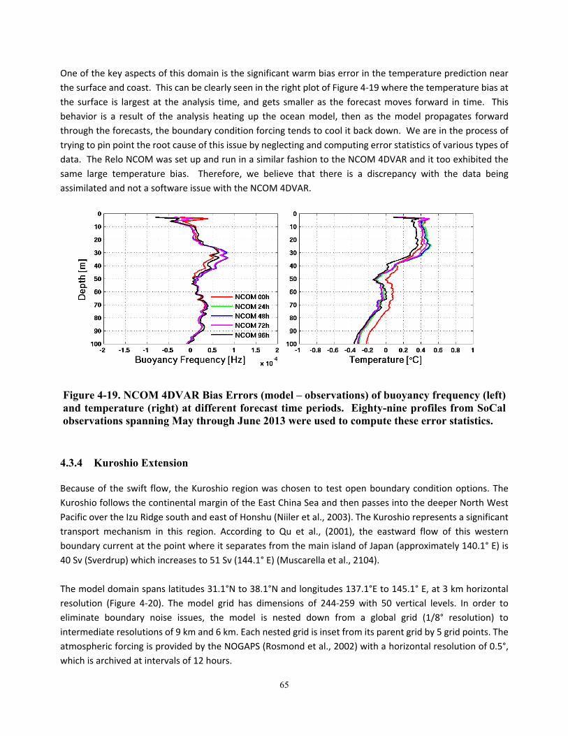
65
One of the key aspects of this domain is the significant warm bias error in the temperature prediction near
the surface and coast. This can be clearly seen in the right plot of Figure 4‐19 where the temperature bias at
the surface is largest at the analysis time, and gets smaller as the forecast moves forward in time. This
behavior is a result of the analysis heating up the ocean model, then as the model propagates forward
through the forecasts, the boundary condition forcing tends to cool it back down. We are in the process of
trying to pin point the root cause of this issue by neglecting and computing error statistics of various types of
data. The Relo NCOM was set up and run in a similar fashion to the NCOM 4DVAR and it too exhibited the
same large temperature bias. Therefore, we believe that there is a discrepancy with the data being
assimilated and not a software issue with the NCOM 4DVAR.
Figure 4-19. NCOM 4DVAR Bias Errors (model – observations) of buoyancy frequency (left) and temperature (right) at different forecast time periods. Eighty-nine profiles from SoCal observations spanning May through June 2013 were used to compute these error statistics.
4.3.4 Kuroshio Extension
Because of the swift flow, the Kuroshio region was chosen to test open boundary condition options. The
Kuroshio follows the continental margin of the East China Sea and then passes into the deeper North West
Pacific over the Izu Ridge south and east of Honshu (Niiler et al., 2003). The Kuroshio represents a significant
transport mechanism in this region. According to Qu et al., (2001), the eastward flow of this western
boundary current at the point where it separates from the main island of Japan (approximately 140.1° E) is
40 Sv (Sverdrup) which increases to 51 Sv (144.1° E) (Muscarella et al., 2104).
The model domain spans latitudes 31.1°N to 38.1°N and longitudes 137.1°E to 145.1° E, at 3 km horizontal
resolution (Figure 4‐20). The model grid has dimensions of 244‐259 with 50 vertical levels. In order to
eliminate boundary noise issues, the model is nested down from a global grid (1/8° resolution) to
intermediate resolutions of 9 km and 6 km. Each nested grid is inset from its parent grid by 5 grid points. The
atmospheric forcing is provided by the NOGAPS (Rosmond et al., 2002) with a horizontal resolution of 0.5°,
which is archived at intervals of 12 hours.
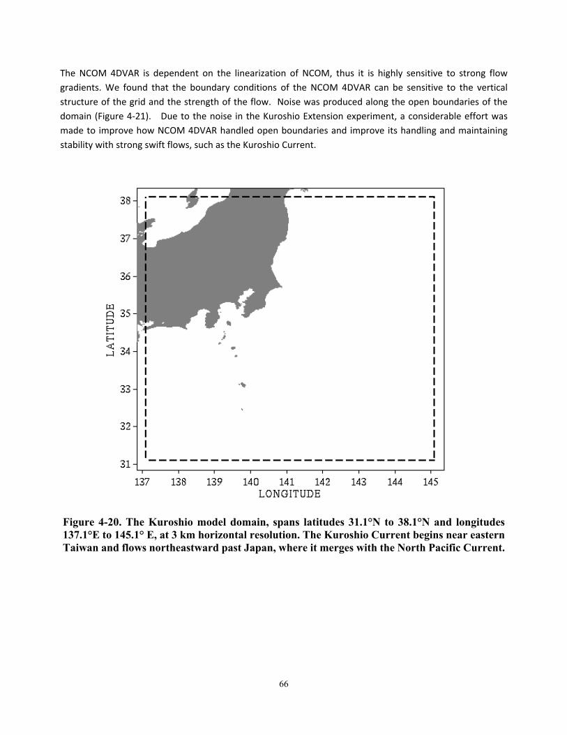
66
The NCOM 4DVAR is dependent on the linearization of NCOM, thus it is highly sensitive to strong flow
gradients. We found that the boundary conditions of the NCOM 4DVAR can be sensitive to the vertical
structure of the grid and the strength of the flow. Noise was produced along the open boundaries of the
domain (Figure 4‐21). Due to the noise in the Kuroshio Extension experiment, a considerable effort was
made to improve how NCOM 4DVAR handled open boundaries and improve its handling and maintaining
stability with strong swift flows, such as the Kuroshio Current.
Figure 4-20. The Kuroshio model domain, spans latitudes 31.1°N to 38.1°N and longitudes 137.1°E to 145.1° E, at 3 km horizontal resolution. The Kuroshio Current begins near eastern Taiwan and flows northeastward past Japan, where it merges with the North Pacific Current.
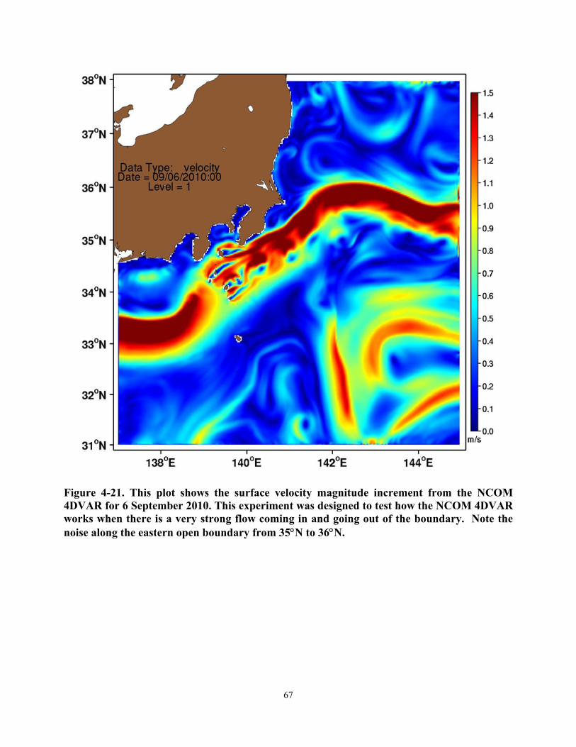
67
Figure 4-21. This plot shows the surface velocity magnitude increment from the NCOM 4DVAR for 6 September 2010. This experiment was designed to test how the NCOM 4DVAR works when there is a very strong flow coming in and going out of the boundary. Note the noise along the eastern open boundary from 35N to 36N.

68
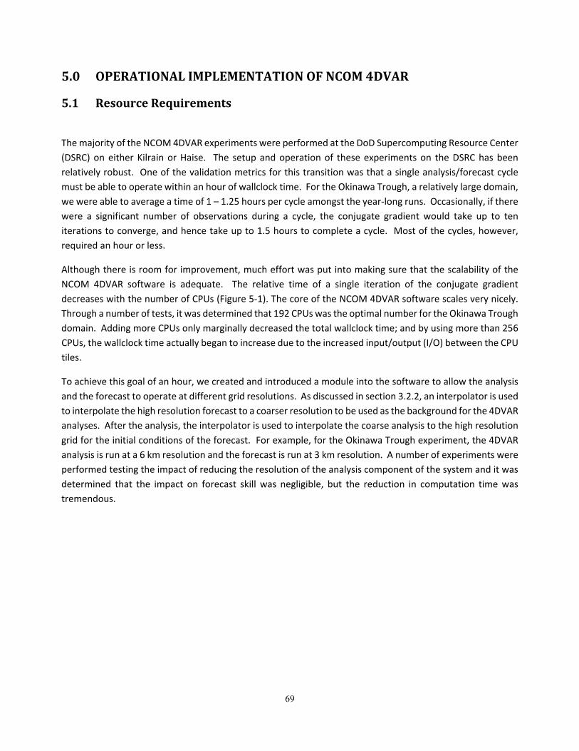
69
5.0 OPERATIONALIMPLEMENTATIONOFNCOM4DVAR
5.1 ResourceRequirements
The majority of the NCOM 4DVAR experiments were performed at the DoD Supercomputing Resource Center
(DSRC) on either Kilrain or Haise. The setup and operation of these experiments on the DSRC has been
relatively robust. One of the validation metrics for this transition was that a single analysis/forecast cycle
must be able to operate within an hour of wallclock time. For the Okinawa Trough, a relatively large domain,
we were able to average a time of 1 – 1.25 hours per cycle amongst the year‐long runs. Occasionally, if there
were a significant number of observations during a cycle, the conjugate gradient would take up to ten
iterations to converge, and hence take up to 1.5 hours to complete a cycle. Most of the cycles, however,
required an hour or less.
Although there is room for improvement, much effort was put into making sure that the scalability of the
NCOM 4DVAR software is adequate. The relative time of a single iteration of the conjugate gradient
decreases with the number of CPUs (Figure 5‐1). The core of the NCOM 4DVAR software scales very nicely.
Through a number of tests, it was determined that 192 CPUs was the optimal number for the Okinawa Trough
domain. Adding more CPUs only marginally decreased the total wallclock time; and by using more than 256
CPUs, the wallclock time actually began to increase due to the increased input/output (I/O) between the CPU
tiles.
To achieve this goal of an hour, we created and introduced a module into the software to allow the analysis
and the forecast to operate at different grid resolutions. As discussed in section 3.2.2, an interpolator is used
to interpolate the high resolution forecast to a coarser resolution to be used as the background for the 4DVAR
analyses. After the analysis, the interpolator is used to interpolate the coarse analysis to the high resolution
grid for the initial conditions of the forecast. For example, for the Okinawa Trough experiment, the 4DVAR
analysis is run at a 6 km resolution and the forecast is run at 3 km resolution. A number of experiments were
performed testing the impact of reducing the resolution of the analysis component of the system and it was
determined that the impact on forecast skill was negligible, but the reduction in computation time was
tremendous.
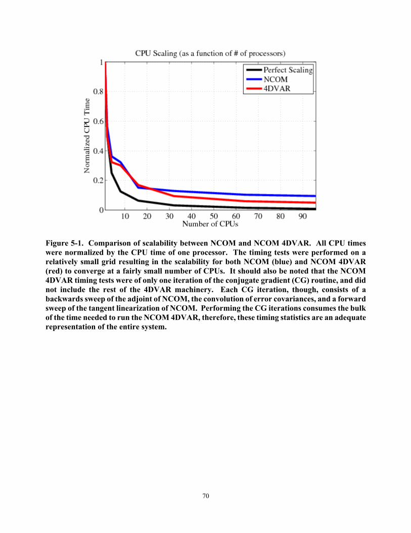
70
Figure 5-1. Comparison of scalability between NCOM and NCOM 4DVAR. All CPU times were normalized by the CPU time of one processor. The timing tests were performed on a relatively small grid resulting in the scalability for both NCOM (blue) and NCOM 4DVAR (red) to converge at a fairly small number of CPUs. It should also be noted that the NCOM 4DVAR timing tests were of only one iteration of the conjugate gradient (CG) routine, and did not include the rest of the 4DVAR machinery. Each CG iteration, though, consists of a backwards sweep of the adjoint of NCOM, the convolution of error covariances, and a forward sweep of the tangent linearization of NCOM. Performing the CG iterations consumes the bulk of the time needed to run the NCOM 4DVAR, therefore, these timing statistics are an adequate representation of the entire system.
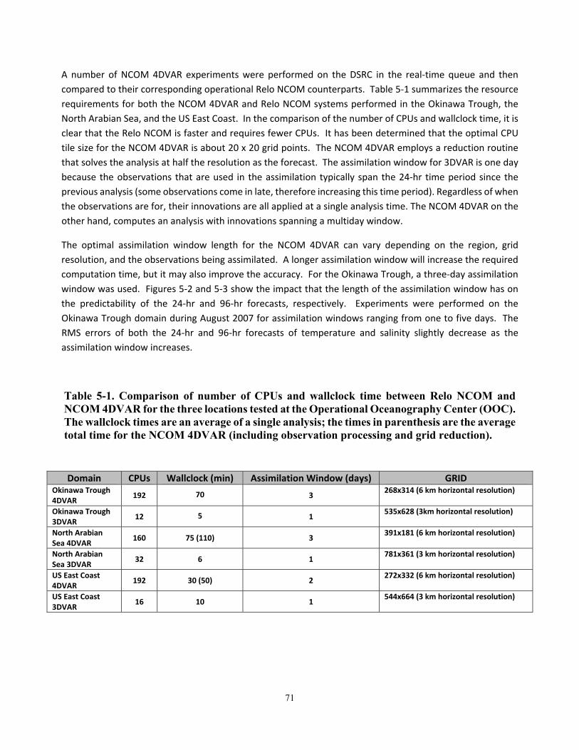
71
A number of NCOM 4DVAR experiments were performed on the DSRC in the real‐time queue and then
compared to their corresponding operational Relo NCOM counterparts. Table 5‐1 summarizes the resource
requirements for both the NCOM 4DVAR and Relo NCOM systems performed in the Okinawa Trough, the
North Arabian Sea, and the US East Coast. In the comparison of the number of CPUs and wallclock time, it is
clear that the Relo NCOM is faster and requires fewer CPUs. It has been determined that the optimal CPU
tile size for the NCOM 4DVAR is about 20 x 20 grid points. The NCOM 4DVAR employs a reduction routine
that solves the analysis at half the resolution as the forecast. The assimilation window for 3DVAR is one day
because the observations that are used in the assimilation typically span the 24‐hr time period since the
previous analysis (some observations come in late, therefore increasing this time period). Regardless of when
the observations are for, their innovations are all applied at a single analysis time. The NCOM 4DVAR on the
other hand, computes an analysis with innovations spanning a multiday window.
The optimal assimilation window length for the NCOM 4DVAR can vary depending on the region, grid
resolution, and the observations being assimilated. A longer assimilation window will increase the required
computation time, but it may also improve the accuracy. For the Okinawa Trough, a three‐day assimilation
window was used. Figures 5‐2 and 5‐3 show the impact that the length of the assimilation window has on
the predictability of the 24‐hr and 96‐hr forecasts, respectively. Experiments were performed on the
Okinawa Trough domain during August 2007 for assimilation windows ranging from one to five days. The
RMS errors of both the 24‐hr and 96‐hr forecasts of temperature and salinity slightly decrease as the
assimilation window increases.
Table 5-1. Comparison of number of CPUs and wallclock time between Relo NCOM and NCOM 4DVAR for the three locations tested at the Operational Oceanography Center (OOC). The wallclock times are an average of a single analysis; the times in parenthesis are the average total time for the NCOM 4DVAR (including observation processing and grid reduction).
Domain CPUs Wallclock (min) Assimilation Window (days) GRID Okinawa Trough 4DVAR
192 70 3 268x314 (6 km horizontal resolution)
Okinawa Trough 3DVAR
12 5 1 535x628 (3km horizontal resolution)
North Arabian Sea 4DVAR
160 75 (110) 3 391x181 (6 km horizontal resolution)
North Arabian Sea 3DVAR
32 6 1 781x361 (3 km horizontal resolution)
US East Coast 4DVAR
192 30 (50) 2 272x332 (6 km horizontal resolution)
US East Coast 3DVAR
16 10 1 544x664 (3 km horizontal resolution)
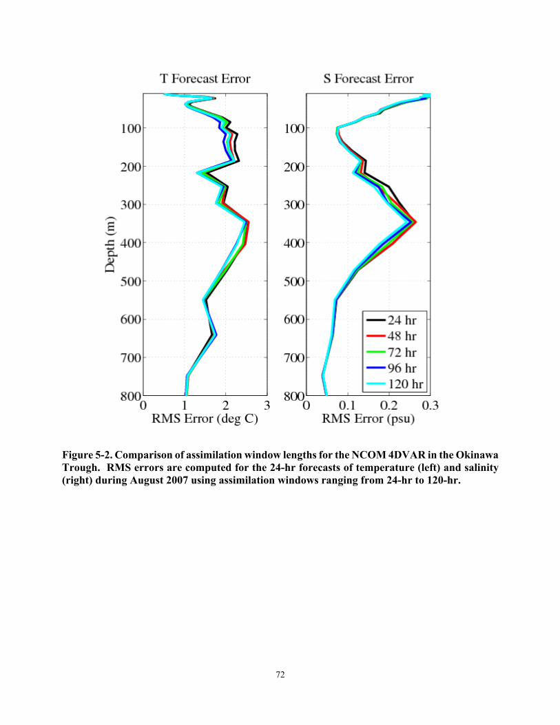
72
Figure 5-2. Comparison of assimilation window lengths for the NCOM 4DVAR in the Okinawa Trough. RMS errors are computed for the 24-hr forecasts of temperature (left) and salinity (right) during August 2007 using assimilation windows ranging from 24-hr to 120-hr.

73
Figure 5-3. Same as Figure 5-2, except comparisons are for the 96-hr forecasts.
5.2 RealTimeDemonstrationontheOOC
In addition to running the domains described in Sections 3 and 4 on the DSRC, three additional experiments
were successfully set up and performed in the same manner, but exclusively in the operational queue on the
DSRC. For a period of several months, we were given a time slot and permission by NAVOCEANO to run the
NCOM 4DVAR in this operational queue. This is a significant achievement, because all of the other
experiments were performed in hindcast; meaning that all of the data, boundary conditions, and forcing files
were already in place prior to the experiments being performed. These additional experiments were
performed in real‐time; meaning that a cycle of the NCOM 4DVAR was performed daily, just following the
acquisition of new data, and the completion of larger model forecasts which provided the forcing and
boundary conditions. It has been demonstrated that the NCOM 4DVAR operated very well in the same
environment in which it will be used operationally.
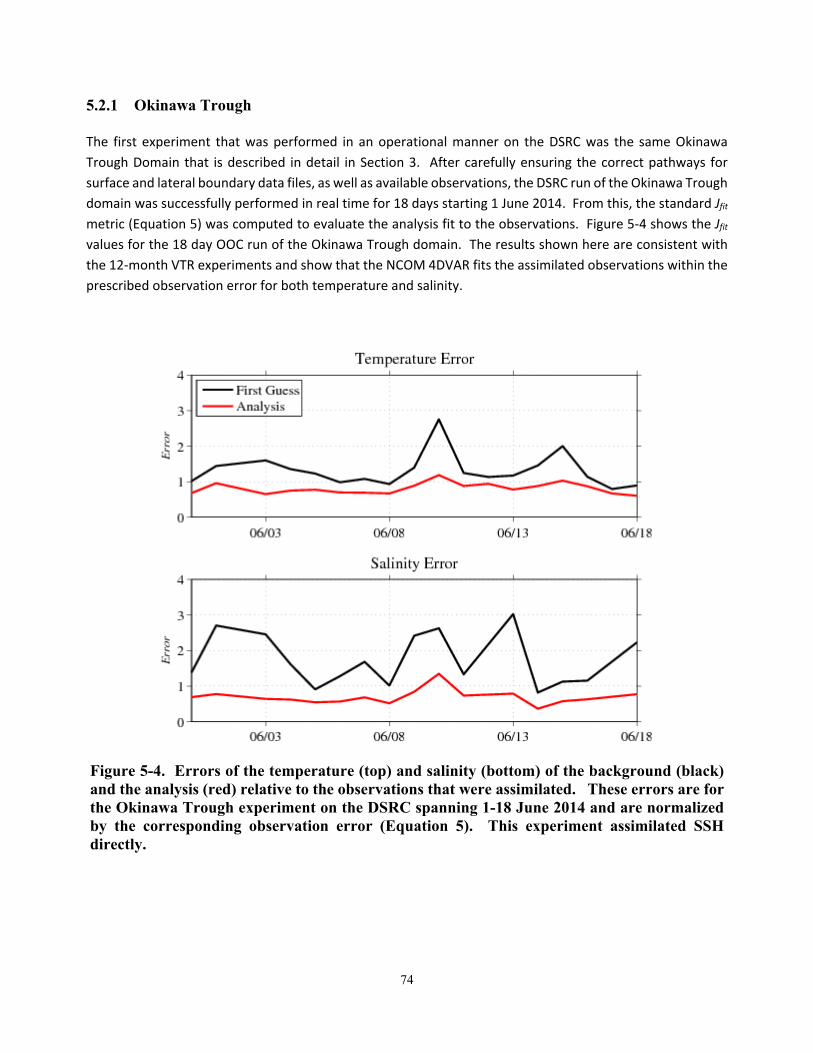
74
5.2.1 Okinawa Trough
The first experiment that was performed in an operational manner on the DSRC was the same Okinawa
Trough Domain that is described in detail in Section 3. After carefully ensuring the correct pathways for
surface and lateral boundary data files, as well as available observations, the DSRC run of the Okinawa Trough
domain was successfully performed in real time for 18 days starting 1 June 2014. From this, the standard Jfit
metric (Equation 5) was computed to evaluate the analysis fit to the observations. Figure 5‐4 shows the Jfit
values for the 18 day OOC run of the Okinawa Trough domain. The results shown here are consistent with
the 12‐month VTR experiments and show that the NCOM 4DVAR fits the assimilated observations within the
prescribed observation error for both temperature and salinity.
Figure 5-4. Errors of the temperature (top) and salinity (bottom) of the background (black) and the analysis (red) relative to the observations that were assimilated. These errors are for the Okinawa Trough experiment on the DSRC spanning 1-18 June 2014 and are normalized by the corresponding observation error (Equation 5). This experiment assimilated SSH directly.
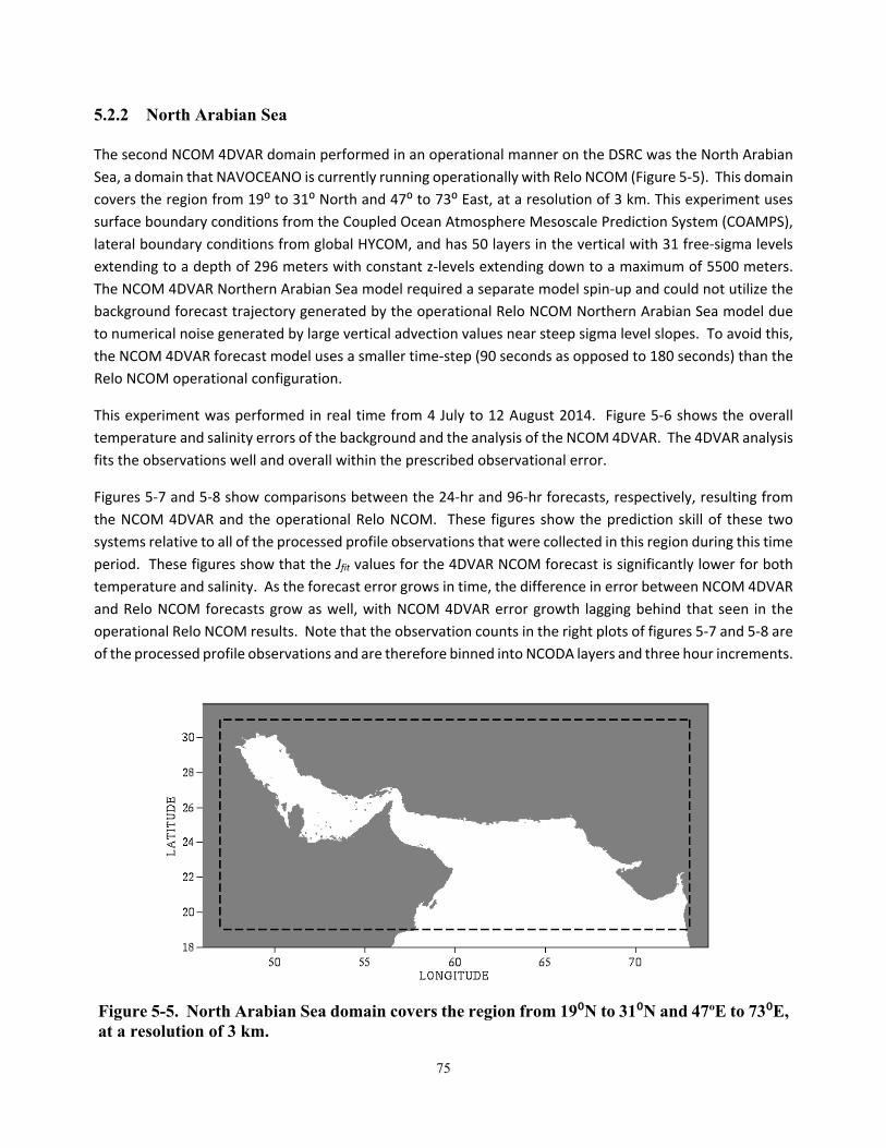
75
5.2.2 North Arabian Sea
The second NCOM 4DVAR domain performed in an operational manner on the DSRC was the North Arabian
Sea, a domain that NAVOCEANO is currently running operationally with Relo NCOM (Figure 5‐5). This domain
covers the region from 19⁰ to 31⁰ North and 47⁰ to 73⁰ East, at a resolution of 3 km. This experiment uses
surface boundary conditions from the Coupled Ocean Atmosphere Mesoscale Prediction System (COAMPS),
lateral boundary conditions from global HYCOM, and has 50 layers in the vertical with 31 free‐sigma levels
extending to a depth of 296 meters with constant z‐levels extending down to a maximum of 5500 meters.
The NCOM 4DVAR Northern Arabian Sea model required a separate model spin‐up and could not utilize the
background forecast trajectory generated by the operational Relo NCOM Northern Arabian Sea model due
to numerical noise generated by large vertical advection values near steep sigma level slopes. To avoid this,
the NCOM 4DVAR forecast model uses a smaller time‐step (90 seconds as opposed to 180 seconds) than the
Relo NCOM operational configuration.
This experiment was performed in real time from 4 July to 12 August 2014. Figure 5‐6 shows the overall
temperature and salinity errors of the background and the analysis of the NCOM 4DVAR. The 4DVAR analysis
fits the observations well and overall within the prescribed observational error.
Figures 5‐7 and 5‐8 show comparisons between the 24‐hr and 96‐hr forecasts, respectively, resulting from
the NCOM 4DVAR and the operational Relo NCOM. These figures show the prediction skill of these two
systems relative to all of the processed profile observations that were collected in this region during this time
period. These figures show that the Jfit values for the 4DVAR NCOM forecast is significantly lower for both
temperature and salinity. As the forecast error grows in time, the difference in error between NCOM 4DVAR
and Relo NCOM forecasts grow as well, with NCOM 4DVAR error growth lagging behind that seen in the
operational Relo NCOM results. Note that the observation counts in the right plots of figures 5‐7 and 5‐8 are
of the processed profile observations and are therefore binned into NCODA layers and three hour increments.
Figure 5-5. North Arabian Sea domain covers the region from 19⁰N to 31⁰N and 47ºE to 73⁰E, at a resolution of 3 km.
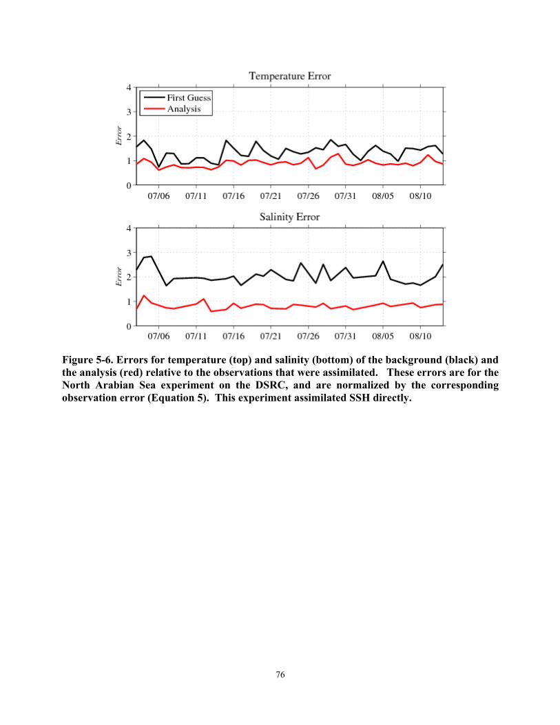
76
Figure 5-6. Errors for temperature (top) and salinity (bottom) of the background (black) and the analysis (red) relative to the observations that were assimilated. These errors are for the North Arabian Sea experiment on the DSRC, and are normalized by the corresponding observation error (Equation 5). This experiment assimilated SSH directly.
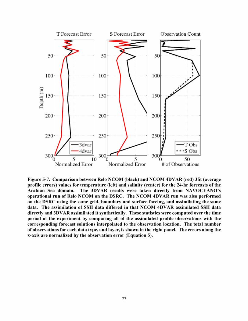
77
Figure 5-7. Comparison between Relo NCOM (black) and NCOM 4DVAR (red) Jfit (average profile errors) values for temperature (left) and salinity (center) for the 24-hr forecasts of the Arabian Sea domain. The 3DVAR results were taken directly from NAVOCEANO’s operational run of Relo NCOM on the DSRC. The NCOM 4DVAR run was also performed on the DSRC using the same grid, boundary and surface forcing, and assimilating the same data. The assimilation of SSH data differed in that NCOM 4DVAR assimilated SSH data directly and 3DVAR assimilated it synthetically. These statistics were computed over the time period of the experiment by comparing all of the assimilated profile observations with the corresponding forecast solutions interpolated to the observation location. The total number of observations for each data type, and layer, is shown in the right panel. The errors along the x-axis are normalized by the observation error (Equation 5).
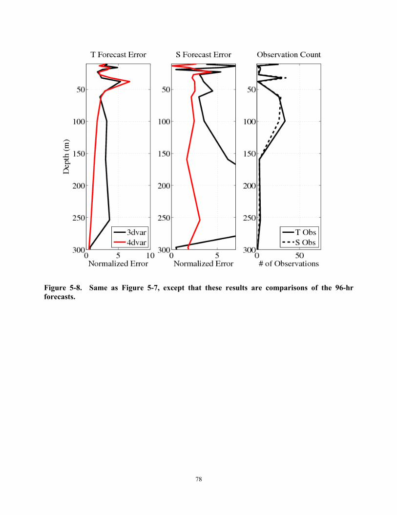
78
Figure 5-8. Same as Figure 5-7, except that these results are comparisons of the 96-hr forecasts.
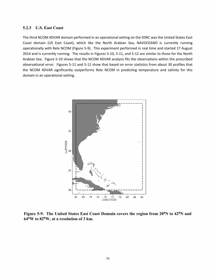
79
5.2.3 U.S. East Coast
The third NCOM 4DVAR domain performed in an operational setting on the DSRC was the United States East
Coast domain (US East Coast), which like the North Arabian Sea, NAVOCEANO is currently running
operationally with Relo NCOM (Figure 5‐9). This experiment performed in real time and started 17 August
2014 and is currently running. The results in Figures 5‐10, 5‐11, and 5‐12 are similar to those for the North
Arabian Sea. Figure 5‐10 shows that the NCOM 4DVAR analysis fits the observations within the prescribed
observational error. Figures 5‐11 and 5‐12 show that based on error statistics from about 30 profiles that
the NCOM 4DVAR significantly outperforms Relo NCOM in predicting temperature and salinity for this
domain in an operational setting.
Figure 5-9. The United States East Coast Domain covers the region from 20⁰N to 42⁰N and 64⁰W to 82⁰W, at a resolution of 3 km.
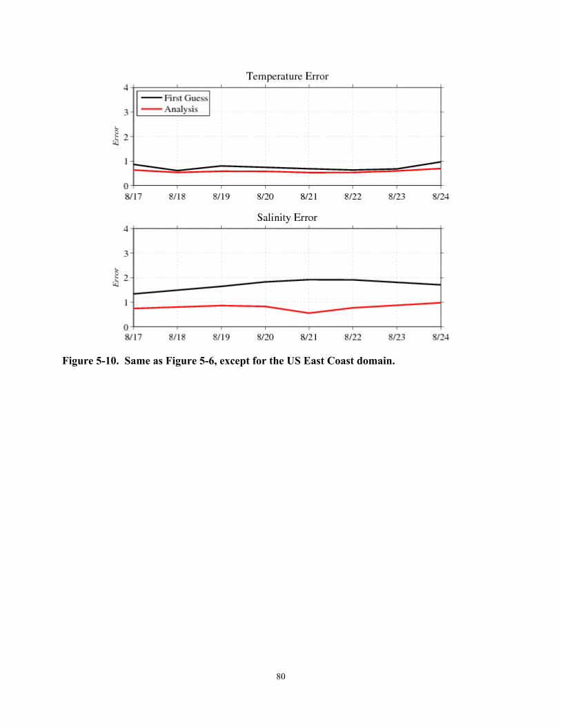
80
Figure 5-10. Same as Figure 5-6, except for the US East Coast domain.
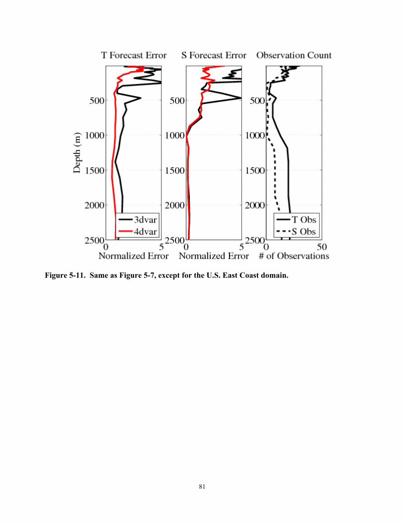
81
Figure 5-11. Same as Figure 5-7, except for the U.S. East Coast domain.
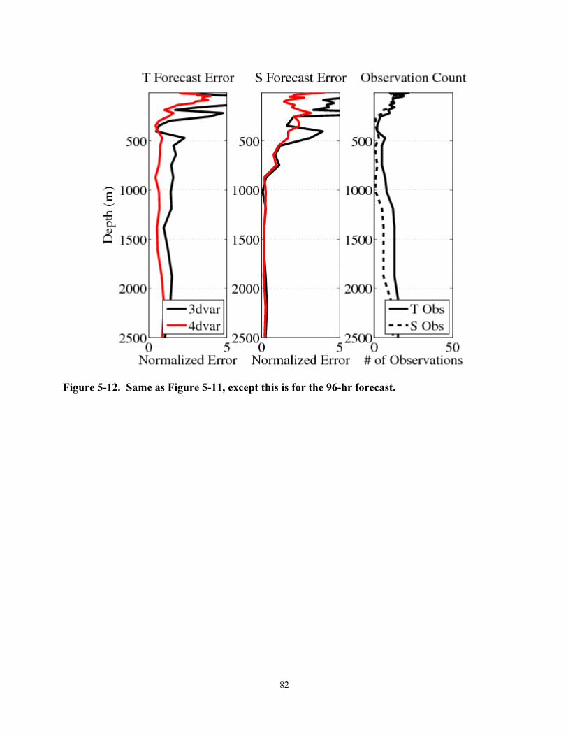
82
Figure 5-12. Same as Figure 5-11, except this is for the 96-hr forecast.
83
6.0 CONCLUSIONS
In this report, the prediction accuracy of NCOM 4DVAR was compared directly to the Relo NCOM
analysis/prediction system primarily for the Okinawa Trough domain. Overall, the results from these
experiments indicate that the NCOM 4DVAR analysis system, when assimilating SSH observations directly or
through synthetic profiles of temperature and salinity, fits the assimilated observations within the prescribed
observation error. Further, the resulting forecasts generated from the NCOM 4DVAR analyses perform
equally or better than the forecasts generated from the Relo NCOM analysis, for subsurface temperature and
salinity, model sea surface height, and mixed layer depth.
In addition to the Okinawa Trough, the NCOM 4DVAR was also performed in the Monterey Bay, the Gulf of
Mexico, the Pacific Rim of Hawaii, the Middle Atlantic Bight, Southern California, and the Kuroshio Extension.
The purpose of these experiments varied, but overall they show that the NCOM 4DVAR system is portable
and can produce good results in regions with varying flow conditions and bottom topography.
Finally, and probably most importantly, three additional experiments were performed on the DSRC in real
time for the Okinawa Trough, the Northern Arabian Sea, and the US East Coast. For the latter two
experiments, results were compared directly with the operational Relo NCOM versions. These comparisons
demonstrated a significant improvement in performance in terms of reduced RMS errors for temperature
and salinity analyses and forecasts.
Overall, the validation results presented in this report reveal that the applications of NCOM 4DVAR has an
improved performance in the prediction skill of temperature, salinity, velocity, SSH, and sonic layer depth
when compared to similar applications of the operational Relo NCOM system.

84
85
7.0 FUTUREWORK
The scope of the NCOM 4DVAR transition, as outlined in this VTR, was to implement an NCOM 4DVAR
assimilation capability into the Relocatable / Regional NCOM system and the COAMPS‐5 system, and test and
validate the NCOM 4DVAR capability in the Okinawa Trough with the 2007 Navy exercise dataset. It is
understood, however, that NAVOCEANO will want to run the NCOM 4DVAR assimilation system in different
domains with different configurations. In addition, NAVOCEANO will want to utilize the capability of the
NCOM 4DVAR system to improve other modeling and assimilation efforts.
The following is a list of all the known projects involving the NCOM 4DVAR system either directly or indirectly.
The development of these efforts range from being in the planning phase to varying stages of completion:
Relocatability: The behavior of the NCOM 4DVAR system depends on the choice of lateral boundary
condition options and correlation scales and errors, and these parameters should change depending
on the domain. Therefore, software needs to be added to automate the selection of these
parameters.
Adaptive Sampling: Similar to what is currently in the NCODA 3DVAR, a module can be added to the
NCOM 4DVAR to perform sensitivity analyses and determine the impact of potential targeted
observations and observation networks.
COAMPS‐OS GUI: All of the software for the NCOM 4DVAR has been added to the COAMPS software
repository. But the capability to operate it directly from the COAMPS‐OS GUI has not been done. This
would be a useful feature.
Improve Efficiency: It is ideal for the code to be able to run as fast as possible. A faster code will
allow for higher resolution or longer forecasts. We have come across several things that that can be
changed to improve the software’s overall efficiency and scalability: Reduce the number of halo
updates, reduce the number of times that arrays are initialized to zero, and implement a more
sophisticated preconditioner for the conjugate gradient.
4DVAR HYCOM: We have begun the planning and proposal phase for building a 4DVAR assimilation
system for HYCOM using the TLM and adjoint of NCOM that is currently in NCOM 4DVAR.
Coupled Ocean‐Wave Assimilative Model: There is an ongoing 6.2 effort to couple the NCOM 4DVAR
with the 4DVAR of Swan in order to extend predictability of currents, waves, and density in shallow
coastal waters through the effective use of in situ observations to influence model predictions.
Heat Flux Corrections: There is an ongoing 6.2 project to add the capability for the NCOM 4DVAR
system to include corrections to the heat flux terms in order to quantify ocean error covariance by
using mismatches with ocean observations to balance error contributions among surface flux and
ocean processes.
Coupled Ocean‐Acoustic Assimilative Model: This is a 6.2 project beginning in FY15 that aims to
reduce acoustic propagation forecast error through a coupled ocean‐acoustic assimilative model.
This coupled system will combine the NCOM 4DVAR with the 4DVAR acoustic model to provide
mutual benefit: The ocean model will benefit from additional acoustic observations, and the acoustic
86
prediction will benefit from the assimilation of direct acoustic observations, indirect observations in
the ocean model, and an improved ocean forecast for making future predictions .
Coupled Ocean‐Atmosphere Variational Assimilation and Prediction System: This is a 6.2 project
beginning in FY15 that aims to provide the Navy with its first coupled ocean‐atmosphere variational
data assimilation (DA) system. This project will merge the 4DVAR capabilities of the atmospheric and
oceanic components of the Coupled Ocean/Atmospheric Mesoscale Prediction System (COAMPS) to
create a coupled 4DVAR DA capability. This will provide the coupled ocean‐atmosphere forecast with
a fully balanced analysis that accounts for all combined observations in both primary fluids (i.e.,
ocean and atmosphere). This coupled DA system will reduce the errors in not only the state
estimation (i.e., nowcast), but in the forecast as well.
There is also an ongoing Validation and Verification (V&V) effort for the Relo NCOM and NCODA‐VAR
systems, which will allow additional comparisons of the NCOM 4DVAR system against configurations
of NCODA‐VAR which may improve upon the operational configurations that were used in this report.
87
8.0 ACKNOWLEDGEMENTS
The authors were supported by the NRL 6.4 NCOM 4DVAR Rapid Transition Project (projects 4727‐04 and
4727‐14), which was managed by both Space and Naval Warfare Systems Command under program element
063207N and the Office of Naval Research under program element 0602435N. Numerical simulations,
performed on Haise and Kilrain at NAVOCEANO, used grants of computer time from the HPCMP under the
Variational Assimilation High Performance Computing (HPC) subproject. The authors would like to thank the
members of the review panel for their time, critical evaluation, and advice: Bruce Lunde and Andrea Mask
(NAVOCEANO), Stephan Howden and Dmitri Netchaev (University of Southern Mississippi), and Timothy
Campbell and Clark Rowley (NRL). The authors also thank the numerous NRL contributors for their support
in developing and validating the prediction systems and software used in this validation effort.

88
89
9.0 REFERENCES
9.1 CitedReferences
Barron, C.N., A.B. Kara, P.J. Martin, R.C. Rhodes, and L.F. Smedstad, (2006). Formulation, implementation,
and examination of vertical coordinate choices in the global Navy Coastal Ocean Model (NCOM). Ocean
Modeling 11, 347‐375, doi:10.1016/j.ocemod.2005.01.004.
Barron C. N., A. B. Kara, A. B., R. C. Rhodes, C. Rowley, and J. F. Shriver, (2007). Validation Test Report for the
1/8° Global Navy Coastal Model Nowcast/Forecast System. NRL Tech Report NRL/MR/7320‐‐07‐9019. Naval
Research Laboratory, Stennis Space Center, MS.
Barron, C.N., L.F. Smedstad, J.M. Dastugue, O.M. Smedstad. (2007). Evaluation of ocean models using
observed and simulated drifter trajectories: Impact of sea surface height on synthetic profiles for data
assimilation. J. Geophys. Res., 112, C07019. doi:10.1029/2006JC002982.
Bennet, A. F., (1992). Inverse Methods in Physical Oceanography. Cambridge University Press, New York,
347 pp.
Bennett, A. F., (2002). Inverse Modeling of the Ocean and Atmosphere. Cambridge University Press, New
York, 234 pp.
Blumberg, A. F. and G. L. Mellor, (1983). Diagnostic and prognostic numerical circulation studies of the South
Atlantic Bight. J. Geophys. Res., 88, 4579‐4592.
Blumberg, A. F. and G. L. Mellor, (1987). A description of a three‐dimensional coastal ocean circulation model.
In: Three‐Dimensional Coastal Ocean Models. N. Heaps, ed., American Union, New York, N.Y. 208 pgs.
Carrier, M.J. and H. Ngodock, (2010). Background‐error correlation model based on implicit solution of a
diffusion Equation. Ocean Modelling 35, 45–53.
Carrier, M., H. Ngodock, S. Smith, G. Jacobs, P. Muscarella, T. Ozgokmen, B. Haus, and B. Lipphardt. (2014).
Impact of Assimilating Ocean Velocity Observations Inferred from Lagrangian Drifter Data Using the NCOM
4DVAR. Mon. Wea. Review, 142, 1509–1524.
Chao, Y, Z.J. Li, J. Farrara, J.C. McWilliams, J. Bellingham, X. Capet, F. Chavez, J.K. Choi, R. Davis, J. Doyle, D.M.
Fratantoni, P. Li, P. Marchesiello, M.A. Moline, J. Paduan, and S. Ramp, (2009). Development,
implementation, and evaluation of a data‐assimilative ocean forecasting system off the central California
coast. Deep‐Sea Research PART II‐Topical Studies in Oceanography, 56(3‐3), 100‐126.
Chua, B.S. and A.F. Bennett, (2001). An inverse ocean modeling system, Ocean Modeling, 3, 137‐165.
Collins‐Sussman, B., B.W. Fitzpatrick, and C.M. Pilato, (2007). Version Control with Subversion: For
Subversion 1.4: (Compiled from r2866). Creative Commons Attribution License.
90
Courtier, P., (1997). Dual formulation of four‐dimensional variational assimilation. Quart. J. Roy. Meteor.
Soc., 123, 2449‐2461.
Cummings, J. A., (2005). Operational Multivariate Ocean Data Assimilation, Quart.
J. Royal Met. Soc., 131, 3583‐3604.
Cummings, J.A., (2011). Ocean data quality control. In A. Schiller and G. Brassington, (Eds.), Operational
Oceanography in the 21st Century. pp. 91‐122. Springer. doi:10.1007/978‐94‐007‐0332‐2_4.
Haley, PJ, P.F.J. Lermusiaux, A.R. Robinson, W.G. Leslie, O. Logoutov, G. Cossarini, X.S. Liang, P. Moreno, S.R.
Ramp, J.D. Doyle, J. Bellingham, F. Chavez, and S. Johnston, (2009). Forecasting and reanalysis in the
Monterey Bay/California Current region for the Autonomous Ocean Sampling Network‐II experiment. Deep‐
Sea Research Part II‐Topical Studies in Oceanography, 56(3‐5), 127‐148.
Helber R.W., C.N. Barron, M.R. Carnes, and R.A. Zingarelli, (2008). Evaluating the sonic layer depth relative to
the mixed layer depth, J. Geophys. Res., 113. doi: 10.1029/2007JC004595.
Helber, R.W., C.N. Barron, M. Gunduz, P.L. Spence, and R.A. Zingarelli, (2010). Acoustic metric assessment for
UUV observation system simulation experiments, U.S. Navy Journal of Underwater Acoustics, 60(1), 101‐124.
Hodur, R.M., (1997). The Naval Research Laboratory’s Coupled Ocean/Atmosphere Mesoscale Prediction
System (COAMPS). Mon. Wea. Review, 125, 1414‐1430.
Hogan, T., and T. Rosmond, (1991). The description of the Navy Operational Global Atmospheric Predictions
System’s spectral forecast model. Mon.Wea. Rev., 119: 1786‐1815.
Jacobs, G.A., C.N. Barron, D.N. Fox, K.R. Whitmer, S. Klingenberger, D. May, and J.P. Blaha, (2002). Operational
Altimeter Sea Level Products. Oceanography 15(1), 13‐21.
Martin P., (2000). Description of the Navy Coastal Ocean Model Version 1.0. NRL report NRL/FR/7322—00‐
9961. NRL Report. Naval Research Laboratory, Stennis Space Center, MS.
Martin, P.J., G. Peggion, and K.J. Yip, (1998). A comparison of several coastal ocean models, NRL Report
NRL/FR/7322‐‐97‐9692. NRL Report. Naval Research Laboratory, Stennis Space Center, MS.
Martin, P.J., C.N. Barron, L.F. Smedstad, A.J. Wallcraft, R.C. Rhodes, T.J. Campbell, C. Rowley, and S.N. Carroll,
(2008). Software Design Description for the Navy Coastal Ocean Model Version 4.0. NRL Report
NRL/MR/7320‐‐08‐9149, Naval Research Laboratory, Stennis Space Center, MS.
Muscarella, P.A., M.J. Carrier, and H.E. Ngodock, (2014). An examination of a multi‐scale three‐dimensional
variational data assimilation scheme in the Kuroshio Extension using the Naval coastal ocean model.
Continental Shelf Research 73, 41–48.
Ngodock, H.E., (2005). Efficient implementation of covariance multiplication for data assimilation with the
representer method. Ocean Modelling 8(3), 237‐251.
91
Ngodock, H.E. and M. Carrier, (2014). A 4DVAR system for the Navy coastal ocean model Part II: Strong and
weak constraints assimilation experiments with real observations in the Monterey Bay. Monthly Weather
Review vol 142 doi:10.1175/MWR‐D‐13‐00220.
Ngodock, H.E., M. Carrier, I. Souopgui, P. Martin, S. Smith, G. Jacobs, and P. Muscarella, (submitted). On the
direct assimilation of along‐track sea surface height observations into a free‐surface ocean model using a
weak constraints four dimensional variational method. Submitted to Quarterly Journal of the Royal
Meotoroligical Society, 2015.
Niiler, P.P., N.A. Maximenko, G.G. Panteleev, T. Yamagata, and D.B. Olson, (2003). Near‐ surface dynamical
structure of the Kuroshio Extension. J. Geophys. Res. 108(C6), 3193.
Pojc, A. C., T. M. Ozgokmen, B. Lipphart, A. C. Haza, B. Haus, G. Jacobs, A. Reniers, J. Olascoaga, E. Ryan, N.
Guillaumc, P. Hogan, A. Kirwan, A. Griffa, and S. Chen, (2013). Grand Lagrangian Deployment (GLAD): Nature
of surface dispersion near the Deepwater Horizon spill. Nature (submitted).
Qu, T., H. Mitsudera, and B. Qui (2001), A climatological view of the Kuroshio/Oyashio System east of Japan.
J. Phys. Oceanogr. 31, 2575–2589.
Roemmich, D. et al., (2001) Argo: The global array of profiling floats. Observing the Oceans in the 21st
Century, C. J. Koblinsky and N. R. Smith, Eds., Melbourne Bureau of Meteorology, 604 pp.
Rosmond T.E. (1992), The design and testing of the Navy Operational Global Atmospheric Prediction System.
Weather and Forecasting, 7, 262‐262.
Rosmond, T. E., J. Teixeria, M. Peng, T. F. Hogan, and R. Pauley (2002), Navy operational global prediction
system (NOGAPS): Forcing for ocean models. Oceanography, 15, 99‐106.
Rowley, Clark (2010), Validation Test Report for the Relo System. NRL Report NRL/MR/7320‐‐10‐9216, Naval
Research Laboratory, Stennis Space Center, MS.
Rowley, Clark (2014), RELO System User’s Guide, In preparation.
Shulman, I., C.R. Wu, J.K. Lewis, J.D. Paduan, L.K. Rosenfeld, J.C. Kindle, S.R. Ramp, and C.A. Collins (2002),
High resolution modeling and data assimilation in the Monterey Bay area. Continental Shelf Research 22,
1129–1151.
Shulman I, C. Rowley, S. Anderson, S. DeRada, J. Kindle, P. Martin, J. Doyle, J. Cummings, S. Ramp, F. Chavez,
D. Frantoni, and R. Davis (2009), Impact of glider data assimilation on the Monterey Bay Model, Deep Sea
Res. 56, 188–198.
Smagorinsky, J. (1963), General circulation experiments with the primitive Equations. I: The basic
experiment. Mon. Wea. Review, 91, 99‐164.
Smith, S.R., J.A. Cummings, C. Rowley, P. Chu, J. Shriver, R. Helber, P. Spence, S. Carroll, and O. M. Smedstad
(2012), Validation Test Report for the Navy Coupled Ocean Data Assimilation 3D Variational Analysis (NCODA‐
92
VAR) System, Version 3.43. NRL Memorandum Report NRL/MR/7320‐11‐9363, Naval Research Laboratory,
Stennis Space Center, MS.
Smith, S.R. et al., (2014). NCOM 4DVAR Version 1.0 User’s Guide.
Weaver, A. and P. Courtier (2001), Correlation modeling on the sphere using a generalized diffusion Equation.
Quart. J. Roy. Meteor. Soc., 127, 1815‐1846.
Yaremchuk, M., M. Carrier, S. Smith, and G. Jacobs (2013), Background error correlation modeling with
diffusion operators. Data Assimilation for Atmospheric, Oceanic and Hydrologic applications, Vol II, S. K. Park
and L. Yaremchuk Xu, Eds., Springer‐Verlag Berlin Heidelberg, doi:10.1007/978‐3‐642‐35088‐7_15.
Yu, P., A. L. Kurapov, G. D. Egbert, J. S. Allen, and A. P. Kosro, (2012). Variational assimilation of HF radar
surface currents in a coastal ocean model off Oregon. Ocean Modelling, 49‐50, 86‐104.
93
9.2 GeneralReferences
Allard, R. A., T. J. Campbell, T. A. Smith, T. G. Jensen, J. A. Cummings, S. Chen, J. Doyle, X. Hong, R.J. Small,
and S.N. Carroll, (2010). Validation Test Report for the Coupled Ocean/Atmosphere Mesoscale Prediction
System (COAMPS) Version 5.0, NRL Report NRL/MR/7320‐‐10‐9283. Naval Research Laboratory, Stennis
Space Center, MS.
Allard, R.A., T.A. Smith, T.G. Jensen, P.Y. Chu, E. Rogers, T.J. Campbell, U.M. Gravois, S.N. Carroll, K. Watson,
S. Gabersek, (2012), Validation Test Report for the Coupled Ocean/Atmosphere Mesoscale Prediction System
(COAMPS) Version 5.0: Ocean/Wave Component Validation. NRL Report NRL/MR/7320‐‐12‐9423. Naval
Research Laboratory, Stennis Space Center, MS.
Barron, C.N., A.B. Kara, H.E. Hurlburt, C. Rowley, and L.F. Smedstad, (2004) Sea surface height predictions
from the Global Navy Coastal Ocean Model (NCOM) during 1998‐2001. J. Atmos. Oceanic Technol., 21(12),
1876‐1894.
Barron, C. N., M. Gunduz, R. W. Helber, G. A. Jacobs, T. L. Townsend (2010), Validation of Ocean Models for
Use in Acoustic Modeling: The Impact of Short‐term Variations in the Western North Pacific. Journal of
Underwater Acoustics, 60(1), 57‐84.
Bleck, R., (2002). An oceanic general circulation model framed in hybrid isopycnic‐Cartesian coordinates.
Ocean Modelling, 4: 55‐88.
Broquet, G., C.A. Edwards, A.M. Moore, B. S. Powell, M. Veneziani, and J.D. Doyle (2009), Application of
4DVARiational data assimilation to the California Current System. Dynamics of Atmospheres and Oceans, 48,
69–92.
Broquet, G., A.M. Moore, H.G. Arango, C.A. Edwards (2011), Corrections to ocean surface forcing in the
California Current System using 4D Variational data assimilation. Ocean Modelling, 36, 116–132.
Canuto, V.M., A. Howard, Y. Cheng, and M.S. Dubovikov, (2001). Ocean turbulence. Part I: One‐point closure
model. Momentum and heat vertical diffusivities. J. Phys. Oceanogr. 31: 1413–1426.
Canuto, V.M., A. Howard, Y. Cheng, and M.S. Dubovikov, (2002). Ocean turbulence. Part II: Vertical
diffusivities of momentum, heat, salt, mass, and passive scalars. J. Phys. Oceanogr. 32: 240–264.
Chen, S., J.A. Cummings, J.D. Doyle, T.R. Holt, R.M. Hodur, C.S. Liou, M. Liu, A. Mirin, J.A. Ridout, J.M. Schmidt,
G. Sugiyama, and W.T. Thompson, (2002). COAMPS Version 3 model description. Naval Research Laboratory,
Monterey, CA, 93943‐5502. 143 pp.
Chen, S., T.J. Campbell, H. Jin, S. Gaberšek, R. M. Hodur, and P. Martin, 2010: Effect of two‐way air‐sea
coupling in high and low wind speed regimes. Mon. Wea. Rev, 138:3579–3602.
Cooper, M. and K. Haines, (1996). Altimetric assimilation with water property conservation. J.Geophys. Res.,
101(C1: 1059‐1077
94
Daley, R. and E. Barker, (2001). NAVDAS—formulation and diagnostics. Mon. Weather Rev., 129: 869–883.
Egbert, G.D. and S. Erofeeva (2002), Efficient inverse modeling of barotropic ocean tides, J. of Ocean and
Atmos. Tech, 19(2), 183–204.
Erwig M., Z. Fu, and B. Pflaum (2007), Parametric Fortran: Program generation in Scientific Computing.
Journal of Software Maintenance and Evolution, 19(3), 155‐182.
Fabbroni, N., N. Pinardi, P. Oddo, P. Lermusiaux, M. de Marte, P‐M. Poulain, (2010). Marine Rapid
Environmental Assessment using RELOcatable nesting in multiscale operational analyses, Geophys. Res.
Abstracts, 12: EGU2010‐8849.
Fox, D.N., C.N. Barron, M.R. Carnes, M. Booda, G. Peggion, and J. V. Gurley (2002), The Modular Ocean Data
Assimilation System, Oceanography, 15, 22‐28.
Halliwell Jr., G.R., (2003). Evaluation of Vertical Coordinate and Vertical Mixing Algorithms in the HYbrid
Coordinate Ocean Model (HYCOM). Ocean Modelling, 7: 285‐322.
Helber R. W., C. N. Barron, M. R. Carnes, and R. A. Zingarelli, (2008) . Evaluating the sonic layer depth relative
to the mixed layer depth, J. Geophys. Res., 113:C07033, doi:10.1029/2007JC004595.
Helber, R. W., C. N. Barron, M. Gunduz, P. L. Spence, and R. A. Zingarelli, (2010). Acoustic metric assessment
for UUV observation system simulation experiments, U.S. Navy Journal of Underwater Acoustics (JUA (USN)),
60(1).
Hill, C., C. DeLuca V. Balaji, M. Suarez, and A. da Silva, (2004). The Architecture of the Earth System Modeling
Framework, Computing in Science and Engineering, 6(1).
Horton, C., M. Clifford, J. Schmitz, and L.H. Kantha, (1997). A realtime oceanographic nowcast/forecast
system for the Mediterranean Sea. J. Geophys. Res., 102(C11): 25123– 25156.
Isoguchi, O., M. Shimada, F. Sakaida, and H. Kawamura (2009), Investigation of Kuroshio‐induced cold‐core
eddy train in the lee of the Izu Islands using high‐resolution satellite images and numerical simulations.
Remote Sens. Environ. 113, 1912–1925.
Kourafalou, V.H., G. Peng, H. Kang, P.J. Hogan, O.M. Smedstad, and R.H. Weisberg, (2009). Evaluation of
Global Ocean Data Assimilation Experiment products on South Florida nested simulations with the Hybrid
Coordinate Ocean Model. Ocean Dynamics, doi:10.1007/s10236‐008‐0160‐7.
Large, W.G., J.C. McWilliams, and S.C. Doney, (1994). Oceanic vertical mixing: A review and a model with a
nonlocal boundary layer parameterization. Rev. Geophys., 32: 363‐403.
Louis, J. F., M. Tiedtke, and J. F. Geleyn, (1981). A short history of the operational PBL‐parameterization at
ECMWF, Workshop on Planetary Boundary Layer Parameterization, 25‐27 Nov. 1981, pp. 59‐79.
95
Martin, P.J., C.N. Barron, L.F. Smedstad, T.J. Campbell, A.J. Wallcraft, R.C. Rhodes, C. Rowley, T.L. Townsend,
and S.N. Carroll, (2008b). “User’s Manual for the Navy Coastal Ocean Model (NCOM) Version 4.0.”
NRL/MR/7320‐‐08‐9151, Ocean Modeling Division, Naval Research Laboratory, Stennis Space Center, MS.
Mellor, G.L. and T. Yamada, (1982). Development of a turbulence closure model for geophysical fluid
problems. Rev. Geophys. Space Phys., 20: 851‐875.
Metzger E.J., O.M. Smedstad and S.N. Carroll, (2009). User's Manual for Global Ocean Forecast System (GOFS)
Version 3.0 (V3.0). NRL Memo. Rpt., NRL/MR/7320—09‐9175 Ocean Modeling Division, Naval Research
Laboratory, Stennis Space Center, MS.
Metzger E.J., H.E. Hulburt, A.J. Wallcraft, J.F. Shriver, T.L. Townsend, O.M. Smedstad, P.G. Thoppil, D.S.
Franklin, G. Peggion, (2010). Validation Test Report for the Global Ocean Forecast System V3.0‐1/12°
HYCOM/NCODA: Phase II. NRL Memo. Rpt., NRL/MR/732‐‐10‐9236, Ocean Modeling Division, Naval Research
Laboratory, Stennis Space Center, MS. pp. 1‐70.
Price, J.F., R.A. Weller, and R. Pinkel, (1986). Diurnal cycling: Observations and models of the upper ocean
response to diurnal heating, cooling and wind mixing. J. Geophys. Res., 91: 8411‐8427.
Pullen, J., J. Doyle, T. Haack, C. Dorman, R. Signell, and C. Lee, (2007). Bora Event Variability and the Role of
Air‐Sea Feedback, J. Geophys. Res., 112 (C3): C03S18.
Smith, T.A., T.J. Campbell, R.A. Allard, and S.N. Carroll, (2010). “User’s Guide for the Coupled Ocean
Atmospheric Mesoscale Prediction System (COAMPS) Version 5.0”. NRL/MR/7320‐‐10‐9208, Ocean Modeling
Division, Naval Research Laboratory, Stennis Space Center, MS.

96
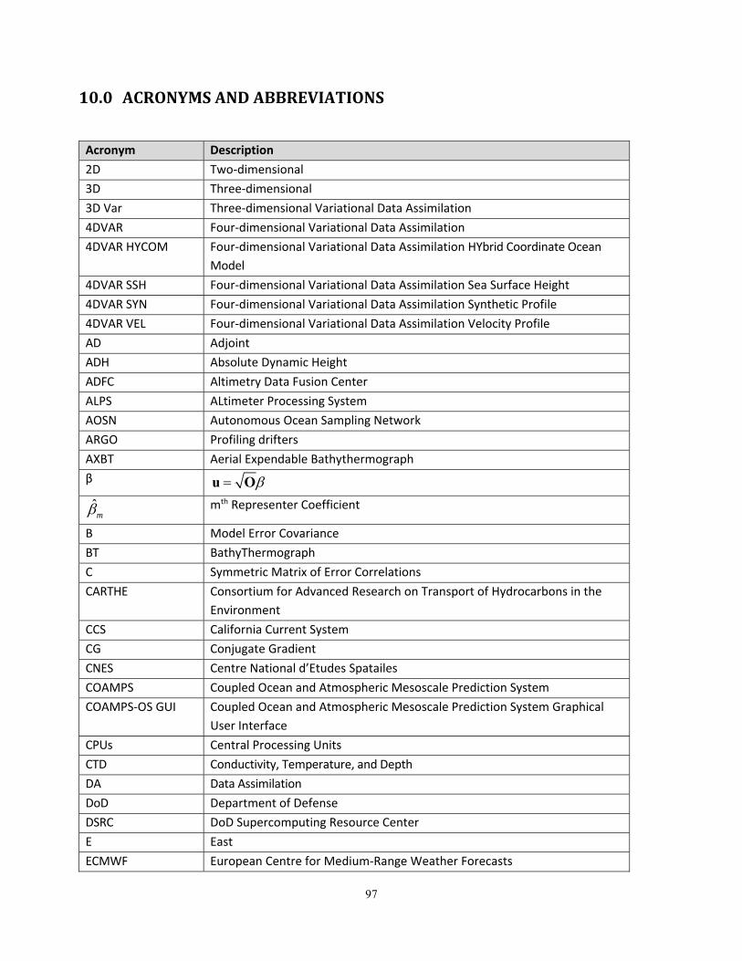
97
10.0 ACRONYMSANDABBREVIATIONS
Acronym Description
2D Two‐dimensional
3D Three‐dimensional
3D Var Three‐dimensional Variational Data Assimilation
4DVAR Four‐dimensional Variational Data Assimilation
4DVAR HYCOM Four‐dimensional Variational Data Assimilation HYbrid Coordinate Ocean
Model
4DVAR SSH Four‐dimensional Variational Data Assimilation Sea Surface Height
4DVAR SYN Four‐dimensional Variational Data Assimilation Synthetic Profile
4DVAR VEL Four‐dimensional Variational Data Assimilation Velocity Profile
AD Adjoint
ADH Absolute Dynamic Height
ADFC Altimetry Data Fusion Center
ALPS ALtimeter Processing System
AOSN Autonomous Ocean Sampling Network
ARGO Profiling drifters
AXBT Aerial Expendable Bathythermograph
β u O
ˆm mth Representer Coefficient
B Model Error Covariance
BT BathyThermograph
C Symmetric Matrix of Error Correlations
CARTHE Consortium for Advanced Research on Transport of Hydrocarbons in the
Environment
CCS California Current System
CG Conjugate Gradient
CNES Centre National d’Etudes Spatailes
COAMPS Coupled Ocean and Atmospheric Mesoscale Prediction System
COAMPS‐OS GUI Coupled Ocean and Atmospheric Mesoscale Prediction System Graphical
User Interface
CPUs Central Processing Units
CTD Conductivity, Temperature, and Depth
DA Data Assimilation
DoD Department of Defense
DSRC DoD Supercomputing Resource Center
E East
ECMWF European Centre for Medium‐Range Weather Forecasts

98
Acronym Description
ENVISAT Environmental Satellite
FNMOC Fleet Numerical Meteorology and Oceanography Command
FR Free Run
GLAD Grand Lagrangian Deployment
GOES Geostationary Operational Environmental Satellite
GOM Gulf of Mexico
GTS Global Telecommunication System
GVC General Vertical Coordinate
H Linear Observation Operator that maps Model Fields and Observation
Locations
Hm OBSERVATION OPERATOR
HPC High Performance Computing
HPCMP High Performance Computing Modernization Program
hr Hour
HYCOM HYbrid Coordinate Ocean Model
Hz Hertz
I/O Input/Output
IP Internet Protocol
Jfit Normalized fit to observations
K Missing co‐efficient
km Kilometers
m Meters
M Total Number of Observations
MAB Middle Atlantic Bight
MB Monterey Bay
MBARI Monterey Bay Aquarium Research Institute
MITgcm Massachusetts Institute of Technology general circulation model
MODAS Modular Ocean Data Assimilation System
MS Mississippi
MT Adjoint of NCOM
MVOI Multi‐Variate Optimum Interpolation
MYL2.5 Mellor‐Yamada (vertical mixing) Level 2.5
N Total number of observations used
N North
NAVDAS NRL Atmospheric Variational Data Assimilation System
NAVGEM Navy Global Environmental Model
NAVOCEANO Naval Oceanographic Office
NCODA Navy Coupled Ocean Data Assimilation
NCODA‐POST Navy Coupled Ocean Data Assimilation Post Processing
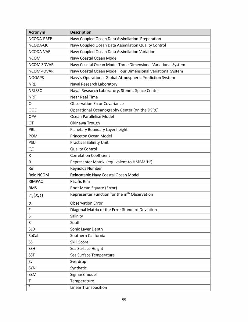
99
Acronym Description
NCODA‐PREP Navy Coupled Ocean Data Assimilation Preparation
NCODA‐QC Navy Coupled Ocean Data Assimilation Quality Control
NCODA‐VAR Navy Coupled Ocean Data Assimilation Variation
NCOM Navy Coastal Ocean Model
NCOM 3DVAR Navy Coastal Ocean Model Three Dimensional Variational System
NCOM 4DVAR Navy Coastal Ocean Model Four Dimensional Variational System
NOGAPS Navy's Operational Global Atmospheric Prediction System
NRL Naval Research Laboratory
NRLSSC Naval Research Laboratory, Stennis Space Center
NRT Near Real Time
O Observation Error Covariance
OOC Operational Oceanography Center (on the DSRC)
OPA Ocean Parallelisé Model
OT Okinawa Trough
PBL Planetary Boundary Layer height
POM Princeton Ocean Model
PSU Practical Salinity Unit
QC Quality Control
R Correlation Coefficient
R Representer Matrix (equivalent to HMBMTHT)
Re Reynolds Number
Relo NCOM Relocatable Navy Coastal Ocean Model
RIMPAC Pacific Rim
RMS Root Mean Square (Error)
( , )mr x t Representer Function for the mth Observation
σm Observation Error
Σ Diagonal Matrix of the Error Standard Deviation
S Salinity
S South
SLD Sonic Layer Depth
SoCal Southern California
SS Skill Score
SSH Sea Surface Height
SST Sea Surface Temperature
Sv Sverdrup
SYN Synthetic
SZM Sigma/Z model
T Temperature T Linear Transposition
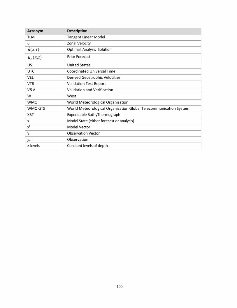
100
Acronym Description
TLM Tangent Linear Model
u Zonal Velocity
ˆ( , )u x t Optimal Analysis Solution
( , )Fu x t Prior Forecast
US United States
UTC Coordinated Universal Time
VEL Derived Geostrophic Velocities
VTR Validation Test Report
V&V Validation and Verification
W West
WMO World Meteorological Organization
WMO GTS World Meteorological Organization Global Telecommunication System
XBT Expendable BathyThermograph
x Model State (either forecast or analysis)
xf Model Vector
y Observation Vector
ym Observation
z‐levels Constant levels of depth
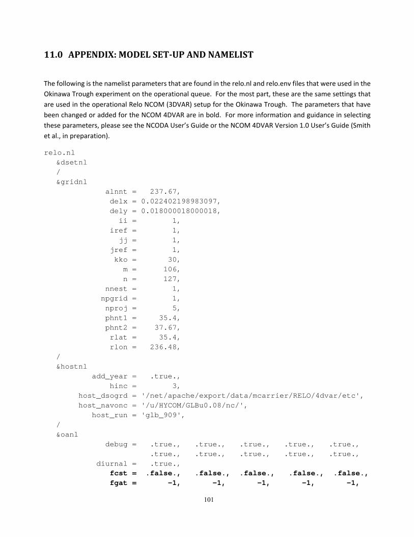
101
11.0 APPENDIX:MODELSET‐UPANDNAMELIST
The following is the namelist parameters that are found in the relo.nl and relo.env files that were used in the
Okinawa Trough experiment on the operational queue. For the most part, these are the same settings that
are used in the operational Relo NCOM (3DVAR) setup for the Okinawa Trough. The parameters that have
been changed or added for the NCOM 4DVAR are in bold. For more information and guidance in selecting
these parameters, please see the NCODA User’s Guide or the NCOM 4DVAR Version 1.0 User’s Guide (Smith
et al., in preparation).
relo.nl &dsetnl / &gridnl alnnt = 237.67, delx = 0.022402198983097, dely = 0.018000018000018, ii = 1, iref = 1, jj = 1, jref = 1, kko = 30, m = 106, n = 127, nnest = 1, npgrid = 1, nproj = 5, phnt1 = 35.4, phnt2 = 37.67, rlat = 35.4, rlon = 236.48, / &hostnl add_year = .true., hinc = 3, host_dsogrd = '/net/apache/export/data/mcarrier/RELO/4dvar/etc', host_navonc = '/u/HYCOM/GLBu0.08/nc/', host_run = 'glb_909', / &oanl debug = .true., .true., .true., .true., .true., .true., .true., .true., .true., .true., diurnal = .true., fcst = .false., .false., .false., .false., .false., fgat = -1, -1, -1, -1, -1,
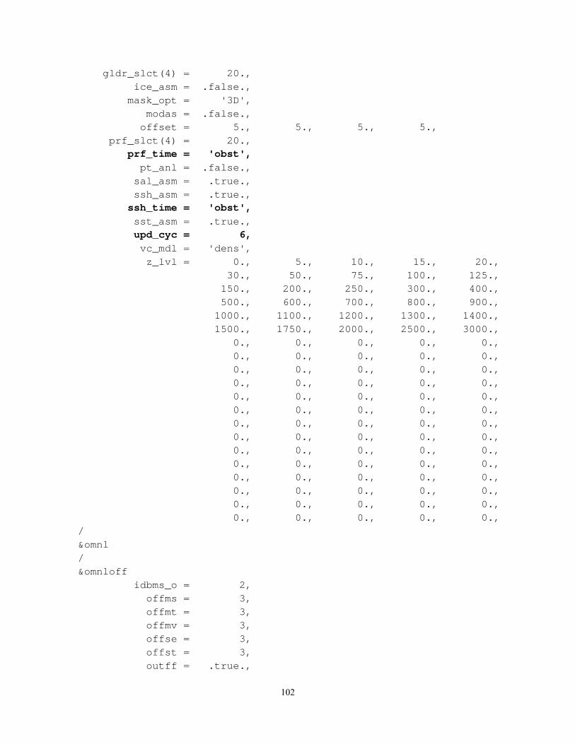
102
gldr_slct(4) = 20., ice_asm = .false., mask_opt = '3D', modas = .false., offset = 5., 5., 5., 5., prf_slct(4) = 20., prf_time = 'obst', pt_anl = .false., sal_asm = .true., ssh_asm = .true., ssh_time = 'obst', sst_asm = .true., upd_cyc = 6, vc_mdl = 'dens', z_lvl = 0., 5., 10., 15., 20., 30., 50., 75., 100., 125., 150., 200., 250., 300., 400., 500., 600., 700., 800., 900., 1000., 1100., 1200., 1300., 1400., 1500., 1750., 2000., 2500., 3000., 0., 0., 0., 0., 0., 0., 0., 0., 0., 0., 0., 0., 0., 0., 0., 0., 0., 0., 0., 0., 0., 0., 0., 0., 0., 0., 0., 0., 0., 0., 0., 0., 0., 0., 0., 0., 0., 0., 0., 0., 0., 0., 0., 0., 0., 0., 0., 0., 0., 0., 0., 0., 0., 0., 0., 0., 0., 0., 0., 0., 0., 0., 0., 0., 0., 0., 0., 0., 0., 0., / &omnl / &omnloff idbms_o = 2, offms = 3, offmt = 3, offmv = 3, offse = 3, offst = 3, outff = .true.,
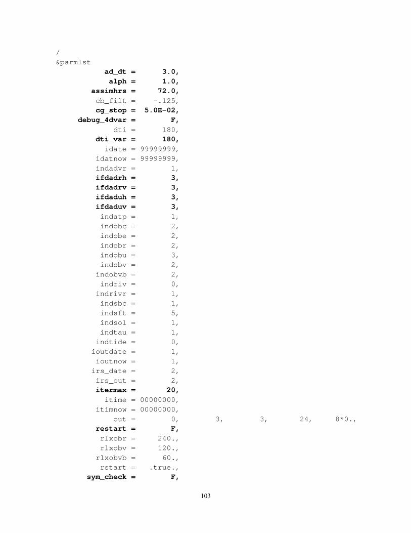
103
/ &parmlst ad_dt = 3.0, alph = 1.0, assimhrs = 72.0, cb_filt = -.125, cg_stop = 5.0E-02, debug_4dvar = F, dti = 180, dti_var = 180, idate = 99999999, idatnow = 99999999, indadvr = 1, ifdadrh = 3, ifdadrv = 3, ifdaduh = 3, ifdaduv = 3, indatp = 1, indobc = 2, indobe = 2, indobr = 2, indobu = 3, indobv = 2, indobvb = 2, indriv = 0, indrivr = 1, indsbc = 1, indsft = 5, indsol = 1, indtau = 1, indtide = 0, ioutdate = 1, ioutnow = 1, irs_date = 2, irs_out = 2, itermax = 20, itime = 00000000, itimnow = 00000000, out = 0, 3, 3, 24, 8*0., restart = F, rlxobr = 240., rlxobv = 120., rlxobvb = 60., rstart = .true., sym_check = F,
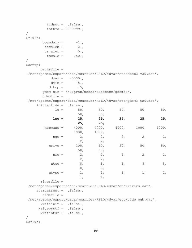
104
tidpot = .false., tothrs = 9999999., / &rlx3nl boundary = -1., tscaleb = 2., tscalei = 5., zscale = 150., / &setupl bathyfile = '/net/apache/export/data/mcarrier/RELO/4dvar/etc/dbdb2_v30.dat', dmax = -5500., dmin = -5., dztop = .5, gdem_dir = '/u/prob/ncoda/database/gdem3s', gdemfile = '/net/apache/export/data/mcarrier/RELO/4dvar/etc/gdem3_ts0.dat', initialtide = .false., lo = 50, 50, 50, 50, 50, 50, 50, lso = 25, 25, 25, 25, 25, 25, 25, nobmaxo = 4000, 4000, 4000, 1000, 1000, 1000, 1000, nqo = 2, 2, 2, 2, 2, 2, 2, nrivo = 200, 50, 50, 50, 50, 50, 50, nro = 2, 2, 2, 2, 2, 2, 2, ntco = 8, 8, 8, 8, 8, 8, 8, ntypo = 1, 1, 1, 1, 1, 1, 1, riverfile = '/net/apache/export/data/mcarrier/RELO/4dvar/etc/rivers.dat', startatrest = .false., tidefile = '/net/apache/export/data/mcarrier/RELO/4dvar/etc/tide_egb.dat', writeinit = .false., writeosstf = .false., writeotsf = .false., / &sflxnl
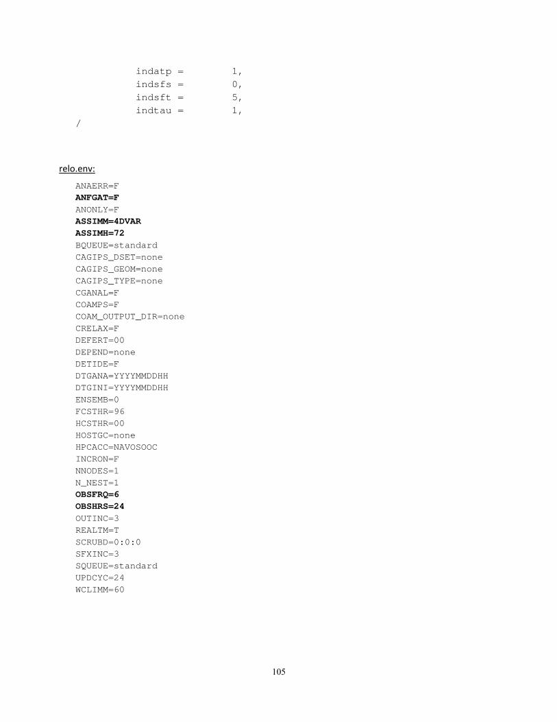
105
indatp = 1, indsfs = 0, indsft = 5, indtau = 1, /
relo.env:
ANAERR=F ANFGAT=F ANONLY=F ASSIMM=4DVAR ASSIMH=72 BQUEUE=standard CAGIPS_DSET=none CAGIPS_GEOM=none CAGIPS_TYPE=none CGANAL=F COAMPS=F COAM_OUTPUT_DIR=none CRELAX=F DEFERT=00 DEPEND=none DETIDE=F DTGANA=YYYYMMDDHH DTGINI=YYYYMMDDHH ENSEMB=0 FCSTHR=96 HCSTHR=00 HOSTGC=none HPCACC=NAVOSOOC INCRON=F NNODES=1 N_NEST=1 OBSFRQ=6 OBSHRS=24 OUTINC=3 REALTM=T SCRUBD=0:0:0 SFXINC=3 SQUEUE=standard UPDCYC=24 WCLIMM=60