Embed Size (px)
Citation preview
Journal of the IEST, V. 55, No. 1 © 2012 10
Validation Techniques for 6-DOF Vibration Data Acquisition
Michael T. Hale and Jesse F. Porter
Dynamic Test Division, Redstone Test Center
Army Test and Evaluation Command
Abstract
Multiple Degree of Freedom (MDOF) excitation systems and MDOF vibration control systems
continue to improve, and are now standard equipment in many dynamic test laboratories. Determination
of an input specification for such MDOF systems is critically dependent on properly acquired field data.
Validation of field data will be discussed and demonstrated employing the same transformation tools used
in both transformation-based 6-degree-of-freedom (6-DOF) vibration control and generalized MDOF
vibration specification development (VSD).
KEYWORDS
Spectral Density Matrix (SDM), 6-degree-of-freedom (6-DOF), acceleration transformation
INTRODUCTION
In this paper, it is assumed that field data are to be collected with the specific intent of either
(1) developing a laboratory setting 6-DOF spectral density matrix (SDM) based input specification,
(2) establishing a time domain reference or set of references for a 6-DOF time waveform replication
(TWR) based test, or (3) simply to measure a 6-DOF event. In all cases, it is critical that the orientation,
position, and scaling associated with each transducer are properly recorded and verified. References to
orientation must be specific with regard to direction and polarity. Use of the traditional right-hand rule for
a Cartesian coordinate system is convenient and strongly recommended to aid in general instrumentation
bookkeeping. Two effective tools will be discussed and are recommended as in-field validation
techniques to ensure 6-DOF field data acquisition efforts will yield valid data sets. The first tool is based
on Cholesky decomposition. The second tool is based on (1) geometric mapping of rigid body motion (as
defined by multiple acceleration measurements) to a single point on the body at which acceleration was
also measured, and (2) comparison of the mapped motion to the measure motion.
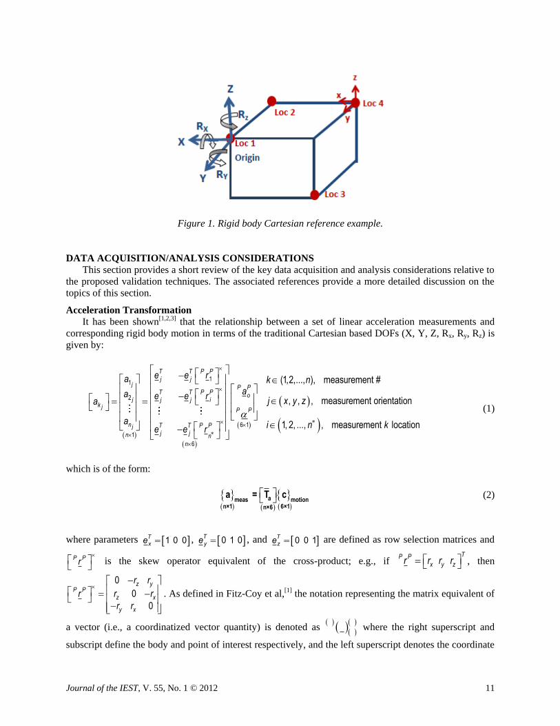
If, at a given instant in time, the translational accelerations at numerous locations on a rigid body are
known, and the relative positions of those locations are known, sufficient information exists to calculate
(or map) the 6-DOF acceleration (translation and rotation) to any point on that body. If the motion is
mapped to a location for which the translational accelerations are known, the mapped accelerations
should match exactly the known accelerations. In the example of Figure 1, the translational accelerations
(x, y, and z) have been measured at four locations on a cube. The 6-DOF acceleration (X, Y, Z, Rx, Ry,
Rz) can then be mapped at the origin, selected to be Location 1. Assuming no position or measurement
error, the mapped acceleration should match the measured acceleration. Failure to match could be an
indication of position or measurement error. This approach can expose scaling, location, orientation, or
polarity errors in a data set.
Journal of the IEST, V. 55, No. 1 © 2012 11
Figure 1. Rigid body Cartesian reference example.
DATA ACQUISITION/ANALYSIS CONSIDERATIONS
This section provides a short review of the key data acquisition and analysis considerations relative to
the proposed validation techniques. The associated references provide a more detailed discussion on the
topics of this section.
Acceleration Transformation
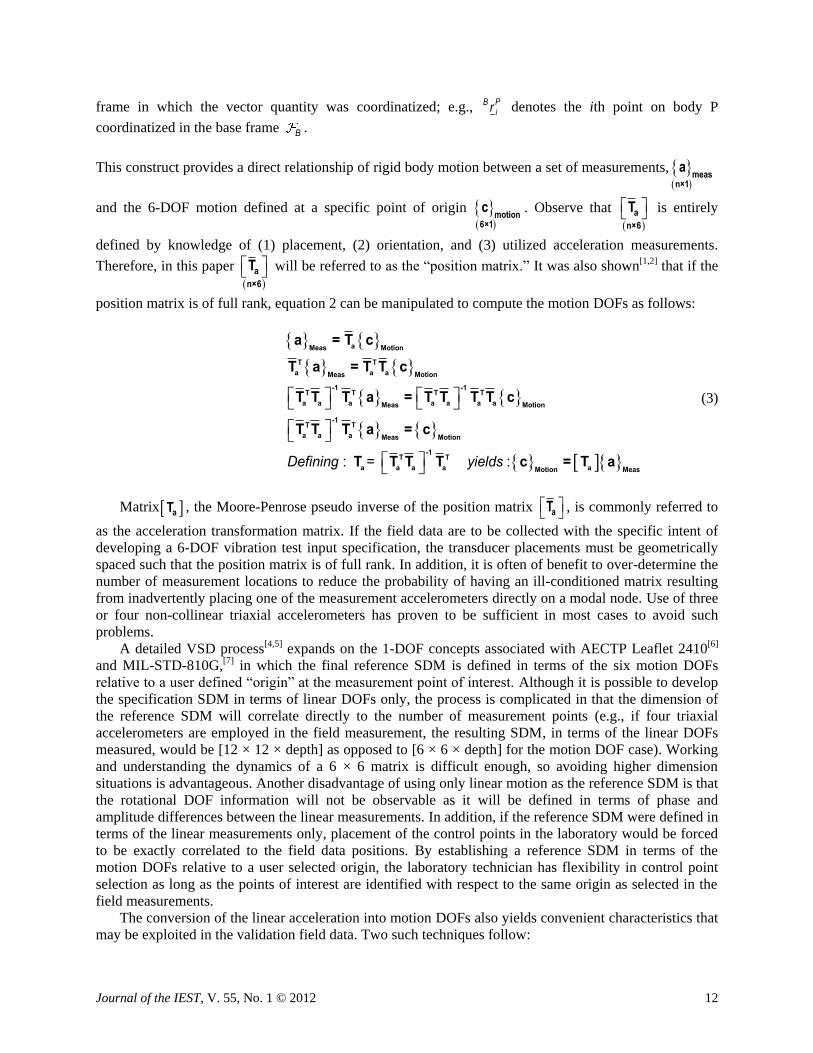
It has been shown[1,2,3] that the relationship between a set of linear acceleration measurements and
corresponding rigid body motion in terms of the traditional Cartesian based DOFs (X, Y, Z, Rx, Ry, Rz) is
given by:
11
2
6 1
1
6
j
j
j
j
T T P P
j j
P PT T P P
oij j
kP P
n T T P P
j jn n
n
e e ra
aa e e ra
ae e r
(1,2,..., ), measurement #
, , , measurement orientation
1, 2, ..., , measurement location
k n
j x y z
i n k
(1)
which is of the form:
ameas motion
n×1 6×1n×6
a = T c (2)
where parameters 1 0 0T
xe , 0 1 0T
ye , and 0 0 1T
ze are defined as row selection matrices and
P Pr is the skew operator equivalent of the cross-product; e.g., if
TP P
x y zr r r r , then
0
0
0
z yP P
z x
y x
r r
r r r
r r
. As defined in Fitz-Coy et al,[1] the notation representing the matrix equivalent of
a vector (i.e., a coordinatized vector quantity) is denoted as
where the right superscript and
subscript define the body and point of interest respectively, and the left superscript denotes the coordinate
Journal of the IEST, V. 55, No. 1 © 2012 12
frame in which the vector quantity was coordinatized; e.g., B P
ir denotes the ith point on body P
coordinatized in the base frame B .
This construct provides a direct relationship of rigid body motion between a set of measurements,
measn×1
a
and the 6-DOF motion defined at a specific point of origin
motion6×1
c . Observe that
a
n×6
T is entirely
defined by knowledge of (1) placement, (2) orientation, and (3) utilized acceleration measurements.
Therefore, in this paper
a
n×6
T will be referred to as the “position matrix.” It was also shown[1,2] that if the
position matrix is of full rank, equation 2 can be manipulated to compute the motion DOFs as follows:
: = :Defining yields
aMeas Motion
T T
a a aMeas Motion
-1 -1T T T T
a a a a a a aMeas Motion
-1T T
a a a Meas Motion
-1T T
a a a a aMotion Meas
a = T c
T a = T T c
T T T a = T T T T c
T T T a = c
T T T T c = T a
(3)
Matrix aT , the Moore-Penrose pseudo inverse of the position matrix aT , is commonly referred to
as the acceleration transformation matrix. If the field data are to be collected with the specific intent of
developing a 6-DOF vibration test input specification, the transducer placements must be geometrically
spaced such that the position matrix is of full rank. In addition, it is often of benefit to over-determine the
number of measurement locations to reduce the probability of having an ill-conditioned matrix resulting
from inadvertently placing one of the measurement accelerometers directly on a modal node. Use of three
or four non-collinear triaxial accelerometers has proven to be sufficient in most cases to avoid such
problems.
A detailed VSD process[4,5] expands on the 1-DOF concepts associated with AECTP Leaflet 2410[6]
and MIL-STD-810G,[7] in which the final reference SDM is defined in terms of the six motion DOFs
relative to a user defined “origin” at the measurement point of interest. Although it is possible to develop
the specification SDM in terms of linear DOFs only, the process is complicated in that the dimension of
the reference SDM will correlate directly to the number of measurement points (e.g., if four triaxial
accelerometers are employed in the field measurement, the resulting SDM, in terms of the linear DOFs
measured, would be [12 × 12 × depth] as opposed to [6 × 6 × depth] for the motion DOF case). Working
and understanding the dynamics of a 6 × 6 matrix is difficult enough, so avoiding higher dimension
situations is advantageous. Another disadvantage of using only linear motion as the reference SDM is that
the rotational DOF information will not be observable as it will be defined in terms of phase and
amplitude differences between the linear measurements. In addition, if the reference SDM were defined in
terms of the linear measurements only, placement of the control points in the laboratory would be forced
to be exactly correlated to the field data positions. By establishing a reference SDM in terms of the
motion DOFs relative to a user selected origin, the laboratory technician has flexibility in control point
selection as long as the points of interest are identified with respect to the same origin as selected in the
field measurements.
The conversion of the linear acceleration into motion DOFs also yields convenient characteristics that
may be exploited in the validation field data. Two such techniques follow:
Journal of the IEST, V. 55, No. 1 © 2012 13
Positive Definite Validation
If the field data acquisition is conducted properly, auto-spectral density (ASD) and cross-spectral
density (CSD) data will be known quantities yielding the ability to compute a fully populated SDM for
each measured event. An SDM is a three-dimensional matrix (row, column, and depth). In this discussion
the depth is frequency. The equations are written as two-dimensional matrices. It is understood that the
calculations will be repeated at each level of depth (frequency lines for the discrete case). An SDM is also
Hermitian *ij ij at each level.
As shown by Nobel[8] and discussed in Smallwood[9] and Hale,[4] an SDM must be positive semi-definite
to be physically realizable. If all the eigenvalues are non-negative, the matrix is positive semi-definite. If
any of the eigenvalues are zero, it implies that one or more of the rows of the SDM are a linear
combination of other rows. In practice, only positive definite matrices are typically encountered. Observe
that even a small amount of noise or nonlinearity will result in a positive definite matrix. If a matrix is
positive definite, the matrix can always be factored using Cholesky decomposition, Φ LL' .
Therefore, by simply computing the SDM of the measured data and then computing a Cholesky
decomposition of the resulting SDM, the data can quickly be verified to be positive definite (or physically
realizable). In measuring a physical event, the resulting SDM should always be positive definite. If the
Cholesky decomposition fails, it is advisable to reevaluate the instrumentation, patching, and signal
conditioning settings.
Mapping to an Instrumented Origin Validation
Mapping to an instrumented origin validation can be utilized only if the geometric positions of the
accelerometers result in a position matrix that is of full rank. It is advantageous to select one of the
reference triaxial translational accelerometers as the user defined origin. This selection allows the data
acquisition team to conduct an acceleration transformation per equation 3 and then perform a direct
comparison between the measured translational data at the origin and the associated mapped motion DOF.
Given that rigidity is assumed, preprocessing the data with a low pass filter at least one octave below the
first mode of the structure of interest is recommended. If the exact frequency of the first mode is
unknown, a conservative low pass filter setting based on geometric characteristics of the measurement
platform is recommended. If the accelerometer orientations (direction and polarity), positions, and scaling
are correct, the measured data at the origin should be highly correlated to the mapped motion DOFs for
each of the translational DOFs being considered. Poor correlation could indicate that the instrumentation,
patching, and signal conditioning settings should be re-evaluated. However, high correlation of
translational DOFs does not necessarily indicate proper instrumentation. Most measurements will not be
of strictly rigid bodies, and making comparisons between mapped translational estimates and translational
data at the origin has the potential to be very close but not exact, thereby potentially masking
instrumentation errors. In some cases the effects of measurement errors, such as improperly scaled
measurements, will be much more apparent in terms of poor correlation of rotational acceleration
computed at the origin via equation 3 and actual measured rotational acceleration. Given the coupled
nature of the angular accelerations, if the translation data matches exactly, the rotational acceleration will
also be correct. This concept will be discussed further and illustrated in the example section of this paper.
In summary, if the measured data at the origin does not match well with the mapped data, it is highly
likely that a mistake was made in the acquisition process. In such cases, it is advisable to re-check the
orientation, position, and scaling descriptions for all transducers prior to proceeding.
EXAMPLES
To illustrate these processes, a series of examples based on measured field data will be discussed.
Although selecting a vehicle such as an armored wheeled vehicle or track vehicle would have the
advantage of being more rigid in nature, a more challenging, relatively flexible rotorcraft data set was
selected to serve as the reference for the following examples. Specifically, the left outboard launcher of a
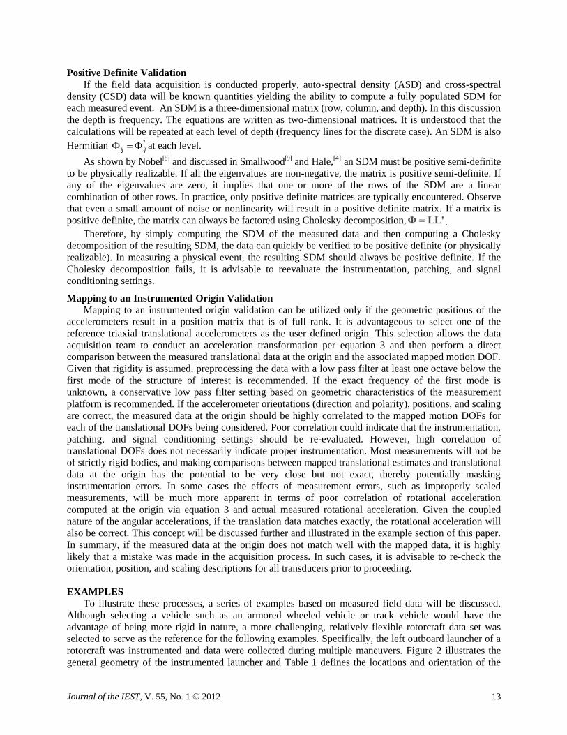
rotorcraft was instrumented and data were collected during multiple maneuvers. Figure 2 illustrates the
general geometry of the instrumented launcher and Table 1 defines the locations and orientation of the
Journal of the IEST, V. 55, No. 1 © 2012 14
acceleration measurements. In a traditional right-hand orientation, the forward direction of the vehicle
was defined as the positive x-axis, from center toward the left pylon was considered the positive y-axis,
and upward through the vehicle roof was considered the positive z-axis. All transducer locations are
referenced in terms of their relative placement to the origin. This location information, along with
orientation, defines the position matrix discussed previously. Observe that the accelerometer orientation
may not always align with the vehicle orientation. The same is true for polarity. For example, the
Launcher Upper Aft Outboard transducer shown in Figure 2 is oriented such that the accelerometer +x,
+y, and +z corresponds to the vehicle +x, -z, and +y directions. It is essential that the field data
acquisition team record such details in a meticulous manner. The orientations and polarities shown in
Table 1 have already been adjusted. The examples shown in this section will address situations in which
orientation, polarity, and scaling errors are made. The purpose is to illustrate the usefulness of in-field
data quality checks.
Figure 2. Instrumented launcher.
Table 1. Transducer location.
Channel and
Orientation
Description Location
X
(inches)
Y
(inches)
Z
(inches)
1x,2y,3z Launcher Lower Outboard Rail 2.250 4.700 -18.250
4x,5y,6z Pylon -27.000 2.950 11.375
7x,8y,9z Bomb Rack, Top Forward Center -6.500 0.000 5.125
10x,11y,12z Launcher Upper Aft Inboard -23.750 -8.25 -4.875
13x,14y,15z Launcher Upper Aft Outboard -23.750 8.25 -4.875
16x,17y,18z Launcher Top Forward Center 0.000 0.000 0.000

Journal of the IEST, V. 55, No. 1 © 2012 15
EXAMPLE INTRODUCTION
For the following examples, the Launcher Top Forward Center location was selected as the origin and
channels 7-18, as defined in Table 1, were employed in the mapping to the origin per equation 3.
Selection of one of the actual measurement locations to serve as the user defined origin allows for direct
comparison between measured translational data at the origin and the data mapped to the origin.
Assuming rigid body motion in the derivation of equation 3, it may be advantageous to conduct the
mapping comparison on a low pass filtered version of the measured data. In all examples, the data were
preprocessed through a low pass filter using Matlab utility filtfilt.m. With the exception of Example 1, the
filter cutoff frequency was set to a conservative 25 Hz. The 200 Hz cutoff frequency of Example 1 also
yielded a good translational match indicating the rigid body assumption was still valid. As the cutoff
frequency is increased, the analysis bandwidth will eventually encompass a structural mode and the
mapping comparison will diverge.
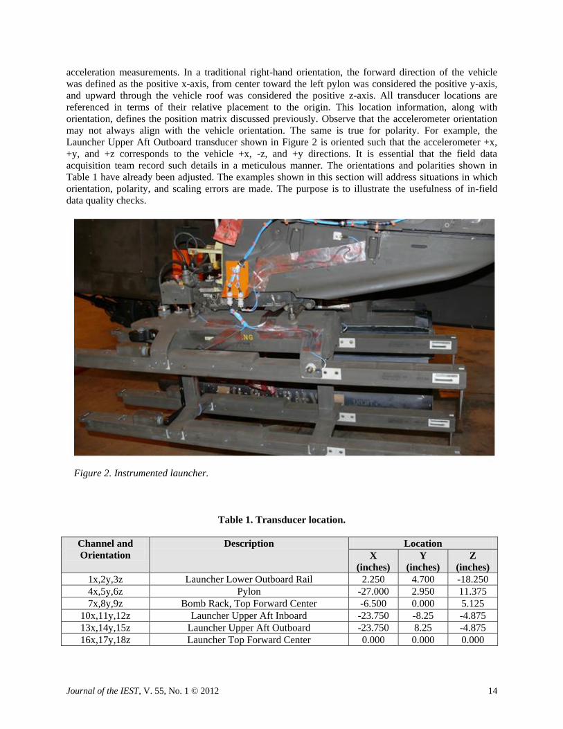
Example 1: Correct Mapping
For Example 1, the low pass filter cutoff frequency was 200 Hz. As illustrated in Figure 3, the
mapped (green) and measured (red) translational data at the origin are highly correlated even at this
relatively wide bandwidth. A clearer view of the data is possible when considering a lower cutoff
frequency, as used in the remaining examples.
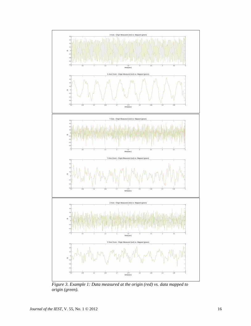
Example 2: Crossed Channel
This example employed the same set of data used in Example 1 with the exception that the X and Y
axes on the acceleration measurements from the Bomb Rack, Top Forward Center locations were
purposely swapped. A quick look at the comparison between mapped and measured translational data at
the origin (Figure 4) indicates a problem. There is poor correlation in both amplitude and phase
characteristics across all three translational axes.
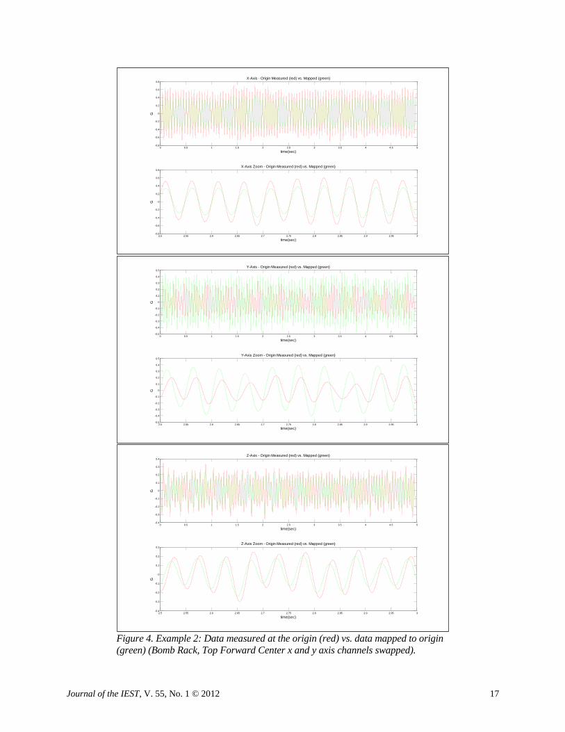
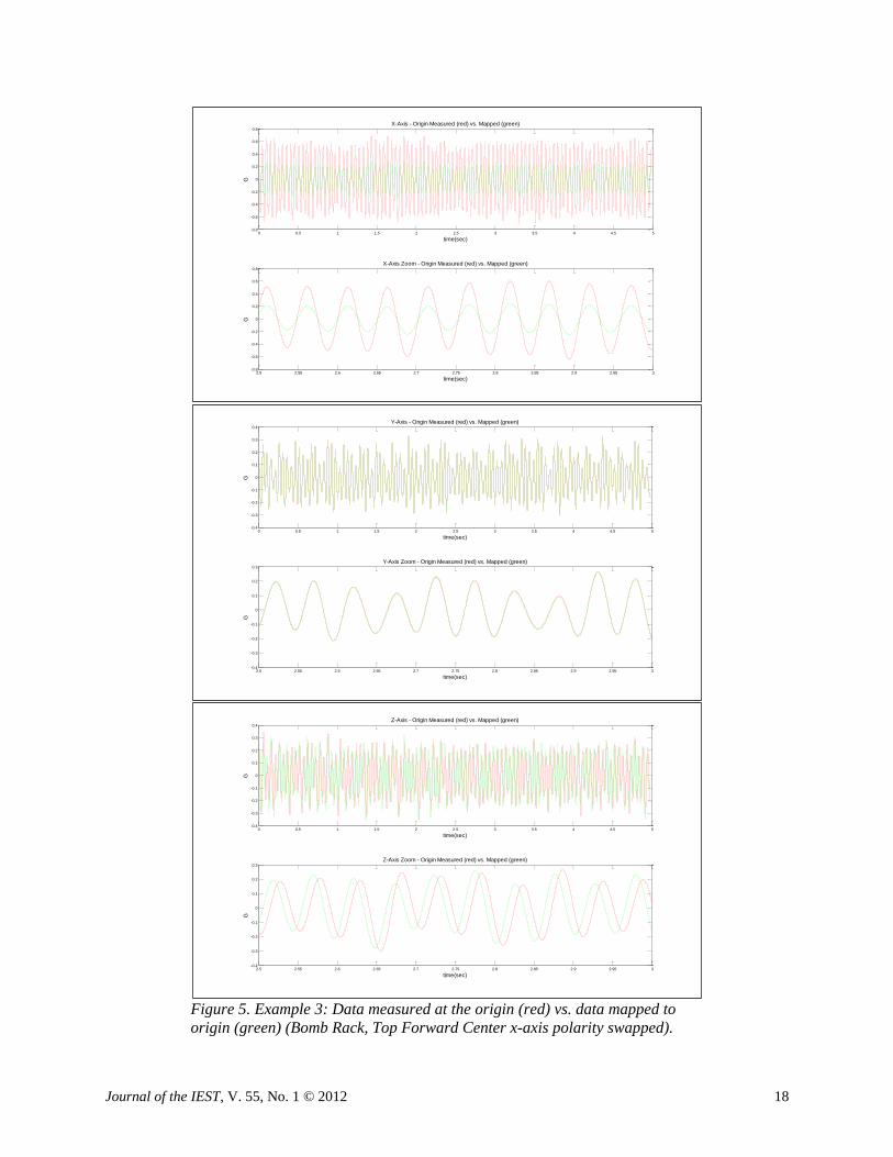
Example 3: Polarity Error
This example employed the same set of data used in Example 1 with the exception that the X-axis
polarity on the acceleration measurement from the Bomb Rack, Top Forward Center location was
purposely swapped. A quick look at the comparison between mapped and measured translational data at
the origin (Figure 5) indicates a problem. There is obviously poor correlation in both amplitude and phase
characteristics in the X and Z axes.
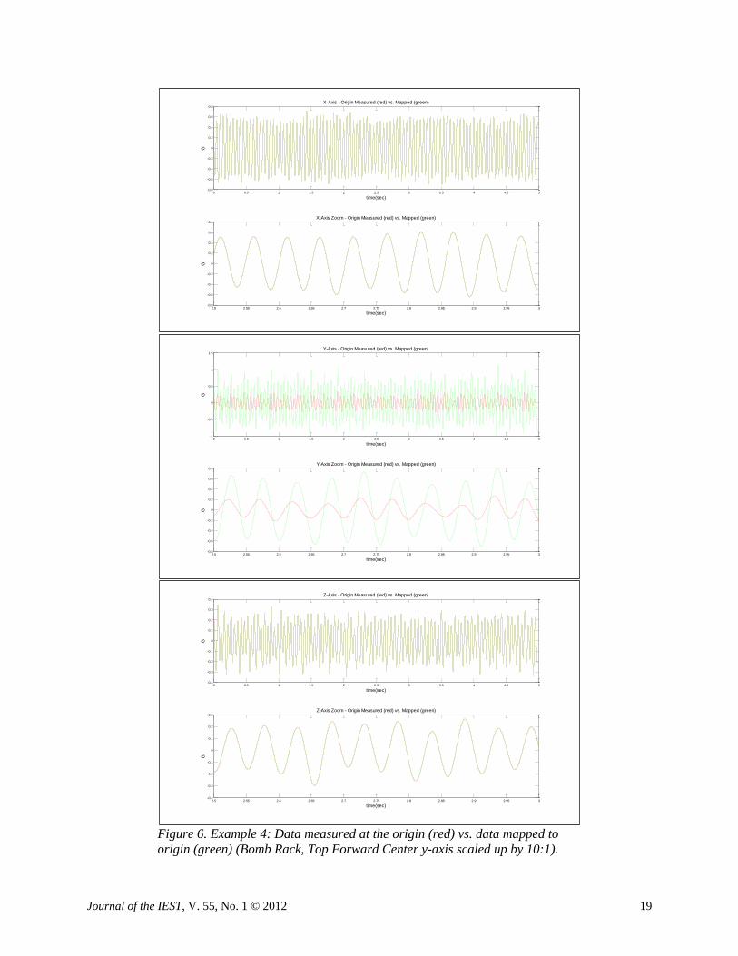
Example 4: Scaling Error I
This example employed the same set of data used in Example 1 with the exception that the Y-axis
acceleration measurement from the Bomb Rack, Top Forward Center location was purposely scaled up by
a factor of 10:1. A quick look at the comparison between mapped and measured translational data at the
origin (Figure 6) indicates a problem. There is poor correlation in both amplitude and phase
characteristics in the Y-axis.
Journal of the IEST, V. 55, No. 1 © 2012 16
Figure 3. Example 1: Data measured at the origin (red) vs. data mapped to
origin (green).
0 0.5 1 1.5 2 2.5 3 3.5 4 4.5 5-0.8
-0.6
-0.4
-0.2
0
0.2
0.4
0.6
0.8
time(sec)G
X-Axis - Origin Measured (red) vs. Mapped (green)
2.5 2.55 2.6 2.65 2.7 2.75 2.8 2.85 2.9 2.95 3-0.8
-0.6
-0.4
-0.2
0
0.2
0.4
0.6
0.8
time(sec)
G
X-Axis Zoom - Origin Measured (red) vs. Mapped (green)
0 0.5 1 1.5 2 2.5 3 3.5 4 4.5 5-1
-0.8
-0.6
-0.4
-0.2
0
0.2
0.4
0.6
0.8
time(sec)
G
Y-Axis - Origin Measured (red) vs. Mapped (green)
2.5 2.55 2.6 2.65 2.7 2.75 2.8 2.85 2.9 2.95 3-0.6
-0.4
-0.2
0
0.2
0.4
0.6
0.8
time(sec)
G
Y-Axis Zoom - Origin Measured (red) vs. Mapped (green)
0 0.5 1 1.5 2 2.5 3 3.5 4 4.5 5-0.6
-0.4
-0.2
0
0.2
0.4
0.6
0.8
time(sec)
G
Z-Axis - Origin Measured (red) vs. Mapped (green)
2.5 2.55 2.6 2.65 2.7 2.75 2.8 2.85 2.9 2.95 3-0.8
-0.6
-0.4
-0.2
0
0.2
0.4
0.6
time(sec)
G
Z-Axis Zoom - Origin Measured (red) vs. Mapped (green)
Journal of the IEST, V. 55, No. 1 © 2012 17
Figure 4. Example 2: Data measured at the origin (red) vs. data mapped to origin
(green) (Bomb Rack, Top Forward Center x and y axis channels swapped).
0 0.5 1 1.5 2 2.5 3 3.5 4 4.5 5-0.8
-0.6
-0.4
-0.2
0
0.2
0.4
0.6
0.8
time(sec)G
X-Axis - Origin Measured (red) vs. Mapped (green)
2.5 2.55 2.6 2.65 2.7 2.75 2.8 2.85 2.9 2.95 3-0.8
-0.6
-0.4
-0.2
0
0.2
0.4
0.6
0.8
time(sec)
G
X-Axis Zoom - Origin Measured (red) vs. Mapped (green)
0 0.5 1 1.5 2 2.5 3 3.5 4 4.5 5-0.5
-0.4
-0.3
-0.2
-0.1
0
0.1
0.2
0.3
0.4
0.5
time(sec)
G
Y-Axis - Origin Measured (red) vs. Mapped (green)
2.5 2.55 2.6 2.65 2.7 2.75 2.8 2.85 2.9 2.95 3-0.5
-0.4
-0.3
-0.2
-0.1
0
0.1
0.2
0.3
0.4
0.5
time(sec)
G
Y-Axis Zoom - Origin Measured (red) vs. Mapped (green)
0 0.5 1 1.5 2 2.5 3 3.5 4 4.5 5-0.4
-0.3
-0.2
-0.1
0
0.1
0.2
0.3
0.4
time(sec)
G
Z-Axis - Origin Measured (red) vs. Mapped (green)
2.5 2.55 2.6 2.65 2.7 2.75 2.8 2.85 2.9 2.95 3-0.4
-0.3
-0.2
-0.1
0
0.1
0.2
0.3
time(sec)
G
Z-Axis Zoom - Origin Measured (red) vs. Mapped (green)
Journal of the IEST, V. 55, No. 1 © 2012 18
Figure 5. Example 3: Data measured at the origin (red) vs. data mapped to
origin (green) (Bomb Rack, Top Forward Center x-axis polarity swapped).
0 0.5 1 1.5 2 2.5 3 3.5 4 4.5 5-0.8
-0.6
-0.4
-0.2
0
0.2
0.4
0.6
0.8
time(sec)G
X-Axis - Origin Measured (red) vs. Mapped (green)
2.5 2.55 2.6 2.65 2.7 2.75 2.8 2.85 2.9 2.95 3-0.8
-0.6
-0.4
-0.2
0
0.2
0.4
0.6
0.8
time(sec)
G
X-Axis Zoom - Origin Measured (red) vs. Mapped (green)
0 0.5 1 1.5 2 2.5 3 3.5 4 4.5 5-0.4
-0.3
-0.2
-0.1
0
0.1
0.2
0.3
0.4
time(sec)
G
Y-Axis - Origin Measured (red) vs. Mapped (green)
2.5 2.55 2.6 2.65 2.7 2.75 2.8 2.85 2.9 2.95 3-0.4
-0.3
-0.2
-0.1
0
0.1
0.2
0.3
time(sec)
G
Y-Axis Zoom - Origin Measured (red) vs. Mapped (green)
0 0.5 1 1.5 2 2.5 3 3.5 4 4.5 5-0.4
-0.3
-0.2
-0.1
0
0.1
0.2
0.3
0.4
time(sec)
G
Z-Axis - Origin Measured (red) vs. Mapped (green)
2.5 2.55 2.6 2.65 2.7 2.75 2.8 2.85 2.9 2.95 3-0.4
-0.3
-0.2
-0.1
0
0.1
0.2
0.3
time(sec)
G
Z-Axis Zoom - Origin Measured (red) vs. Mapped (green)
Journal of the IEST, V. 55, No. 1 © 2012 19
Figure 6. Example 4: Data measured at the origin (red) vs. data mapped to
origin (green) (Bomb Rack, Top Forward Center y-axis scaled up by 10:1).
0 0.5 1 1.5 2 2.5 3 3.5 4 4.5 5-0.8
-0.6
-0.4
-0.2
0
0.2
0.4
0.6
0.8
time(sec)G
X-Axis - Origin Measured (red) vs. Mapped (green)
2.5 2.55 2.6 2.65 2.7 2.75 2.8 2.85 2.9 2.95 3-0.8
-0.6
-0.4
-0.2
0
0.2
0.4
0.6
0.8
time(sec)
G
X-Axis Zoom - Origin Measured (red) vs. Mapped (green)
0 0.5 1 1.5 2 2.5 3 3.5 4 4.5 5-1
-0.5
0
0.5
1
1.5
time(sec)
G
Y-Axis - Origin Measured (red) vs. Mapped (green)
2.5 2.55 2.6 2.65 2.7 2.75 2.8 2.85 2.9 2.95 3-0.8
-0.6
-0.4
-0.2
0
0.2
0.4
0.6
0.8
time(sec)
G
Y-Axis Zoom - Origin Measured (red) vs. Mapped (green)
0 0.5 1 1.5 2 2.5 3 3.5 4 4.5 5-0.4
-0.3
-0.2
-0.1
0
0.1
0.2
0.3
0.4
time(sec)
G
Z-Axis - Origin Measured (red) vs. Mapped (green)
2.5 2.55 2.6 2.65 2.7 2.75 2.8 2.85 2.9 2.95 3-0.4
-0.3
-0.2
-0.1
0
0.1
0.2
0.3
time(sec)
G
Z-Axis Zoom - Origin Measured (red) vs. Mapped (green)

Journal of the IEST, V. 55, No. 1 © 2012 20
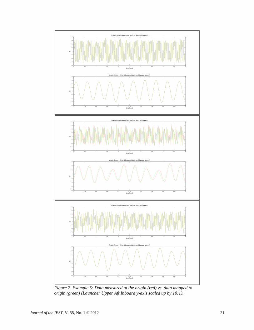
Example 5: Scaling Error II
In each of the previous examples involving induced errors, it was possible to suspect a problem based
solely on comparisons to measured translational data at the origin. As discussed previously, high
correlation of translational DOFs is not a guarantee of proper instrumentation. In such cases, a
comparison of the rotational acceleration can often reveal problems not otherwise found. The intent of
Example 5 is to illustrate that point.
This example employed the same set of data used in Example 1 with the exception that the Y-axis
acceleration measurement from the Launcher Upper Aft Inboard location was purposely scaled up by a
factor of 10:1. This is similar to the error induced in Example 4 except the affected accelerometer is
further from the origin. A visual comparison between mapped and measured translational data at the
origin (Figure 7) does not indicate an obvious problem, and one might wrongly conclude the data are
correct. Due to the increased distance between the affected accelerometer and the origin, the component
in the acceleration transformation matrix that operates on the Y-axis acceleration has minimal effect on
the Y-Axis approximation at the origin. This shortcoming could be overcome by a comparison of the
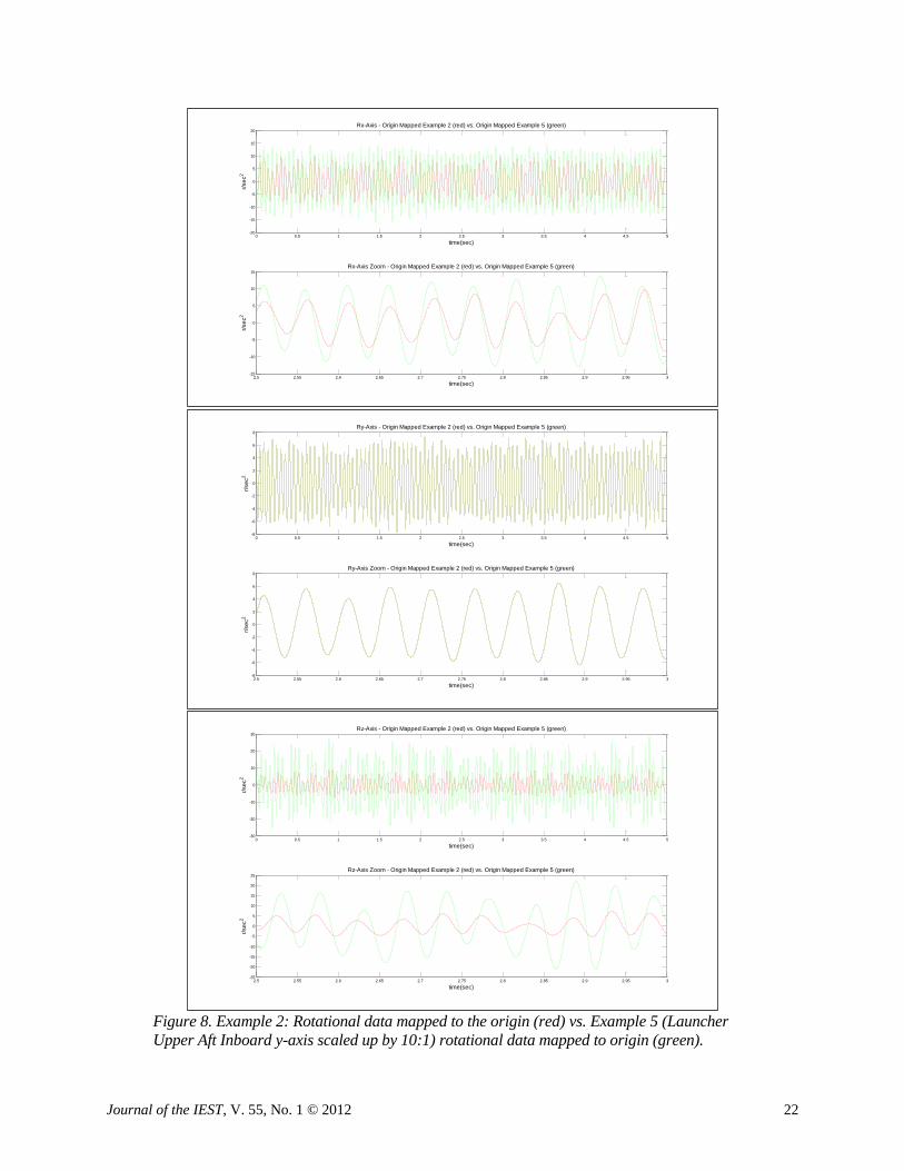
rotational DOFs. It should be noted that this set of test data did not include an angular accelerometer to
which direct angular acceleration mappings could be compared. For illustration purposes in the absence
of measured angular acceleration data, the rotational data mapped to the origin from Example 1, low pass
filtered at 25 Hz, will be used as the reference signal for comparison purposes with the angular data
mapped to the origin given the scaling error of Example 5. Observe that although the translational data
mapped fairly well as shown in Figure 7, the 10:1 scaling error of Example 5 results in significant error in
the rotational estimates Rx and Rz as illustrated in Figure 8. This example provides a good argument for
including at least one angular accelerometer in the data acquisition exercise to which rotational mapped
data could be directly compared.
Example Summary
The previous examples illustrate that many, but not all, instrumentation errors can be discovered by
comparing mapped translational acceleration to measured translation acceleration at the origin. The addition
of angular transducers at the origin provides even stronger tools to validate 6-DOF acceleration data.
It is also important to keep in mind that all of the mapping exercises in the previous examples were
based on the assumption of rigid body motion. In practice, we seldom have the luxury of working with a
rigid body, nor is it ever likely that when we move to the laboratory to implement a 6-DOF vibration test
that the impedance between the field and laboratory conditions will be equivalent. This is why we
generally over-determine the feedback in measuring or controlling MDOF vibration environments as
opposed to simply placing a translational tri-axial accelerometer and a rotational tri-axial accelerometer at
one point to make a 6-DOF measurement. If there are more control channels than rigid body degrees of
freedom, and an input transformation matrix is defined to transform the control accelerometers into rigid
body modes, the motion of each rigid body mode is essentially defined as a weighted average of the
accelerometers active for the mode. In many cases, given the control authority of the shakers, this is the
best viable solution. This approach is analogous to averaging accelerometers for a single axis test, which
is common practice. The elastic modes are not controlled, since often the control authority over these
modes does not exist. The system is driven with an equivalent rigid body motion in each of the rigid body
modes.[4,5,9]
Journal of the IEST, V. 55, No. 1 © 2012 21
Figure 7. Example 5: Data measured at the origin (red) vs. data mapped to
origin (green) (Launcher Upper Aft Inboard y-axis scaled up by 10:1).
0 0.5 1 1.5 2 2.5 3 3.5 4 4.5 5-0.8
-0.6
-0.4
-0.2
0
0.2
0.4
0.6
0.8
time(sec)G
X-Axis - Origin Measured (red) vs. Mapped (green)
2.5 2.55 2.6 2.65 2.7 2.75 2.8 2.85 2.9 2.95 3-0.8
-0.6
-0.4
-0.2
0
0.2
0.4
0.6
0.8
time(sec)
G
X-Axis Zoom - Origin Measured (red) vs. Mapped (green)
0 0.5 1 1.5 2 2.5 3 3.5 4 4.5 5-0.4
-0.3
-0.2
-0.1
0
0.1
0.2
0.3
0.4
time(sec)
G
Y-Axis - Origin Measured (red) vs. Mapped (green)
2.5 2.55 2.6 2.65 2.7 2.75 2.8 2.85 2.9 2.95 3-0.4
-0.3
-0.2
-0.1
0
0.1
0.2
0.3
time(sec)
G
Y-Axis Zoom - Origin Measured (red) vs. Mapped (green)
0 0.5 1 1.5 2 2.5 3 3.5 4 4.5 5-0.4
-0.3
-0.2
-0.1
0
0.1
0.2
0.3
0.4
time(sec)
G
Z-Axis - Origin Measured (red) vs. Mapped (green)
2.5 2.55 2.6 2.65 2.7 2.75 2.8 2.85 2.9 2.95 3-0.4
-0.3
-0.2
-0.1
0
0.1
0.2
0.3
time(sec)
G
Z-Axis Zoom - Origin Measured (red) vs. Mapped (green)
Journal of the IEST, V. 55, No. 1 © 2012 22
Figure 8. Example 2: Rotational data mapped to the origin (red) vs. Example 5 (Launcher
Upper Aft Inboard y-axis scaled up by 10:1) rotational data mapped to origin (green).
0 0.5 1 1.5 2 2.5 3 3.5 4 4.5 5-20
-15
-10
-5
0
5
10
15
20
time(sec)r/
se
c2
Rx-Axis - Origin Mapped Example 2 (red) vs. Origin Mapped Example 5 (green)
2.5 2.55 2.6 2.65 2.7 2.75 2.8 2.85 2.9 2.95 3-15
-10
-5
0
5
10
15
time(sec)
r/se
c2
Rx-Axis Zoom - Origin Mapped Example 2 (red) vs. Origin Mapped Example 5 (green)
0 0.5 1 1.5 2 2.5 3 3.5 4 4.5 5-8
-6
-4
-2
0
2
4
6
8
time(sec)
r/se
c2
Ry-Axis - Origin Mapped Example 2 (red) vs. Origin Mapped Example 5 (green)
2.5 2.55 2.6 2.65 2.7 2.75 2.8 2.85 2.9 2.95 3-8
-6
-4
-2
0
2
4
6
8
time(sec)
r/se
c2
Ry-Axis Zoom - Origin Mapped Example 2 (red) vs. Origin Mapped Example 5 (green)
0 0.5 1 1.5 2 2.5 3 3.5 4 4.5 5-30
-20
-10
0
10
20
30
time(sec)
r/se
c2
Rz-Axis - Origin Mapped Example 2 (red) vs. Origin Mapped Example 5 (green)
2.5 2.55 2.6 2.65 2.7 2.75 2.8 2.85 2.9 2.95 3-25
-20
-15
-10
-5
0
5
10
15
20
25
time(sec)
r/se
c2
Rz-Axis Zoom - Origin Mapped Example 2 (red) vs. Origin Mapped Example 5 (green)

Journal of the IEST, V. 55, No. 1 © 2012 23
CONCLUSIONS
Development of a set of robust tools for validation of data intended for use in an MDOF scenario has
the potential to greatly reduce the need for repeating expensive field data acquisition projects. It is highly
recommended that data to be used in the development of a Multiple Exciter Test (MET) be carefully
validated to ensure the underlying physics of the data is sound at the time of acquisition. A time domain
data validation technique for MDOF data acquisition has been discussed and demonstrated. The technique
illustrated was generally successful in identifying suspect data resulting from common instrumentation-
related mistakes. While the instrumentation technician may be alerted to the possibility of an
instrumentation error, the process shown did not provide an automated process for identifying
problematic channels. Frequency domain techniques based on modal characteristics are expected to
enhance this process.
The same tools may be used to verify that the underlying physics of data delivered from a third party
is sound. In the review of third-party data subsequent to the acquisition effort, an automated tool for
identification of most likely problematic channels would certainly aid the analyst in identifying the
potential source of error. In addition, such tools, especially those developed to operate in the frequency
domain, could also be applied to laboratory MDOF control scenarios to aid in identification of
instrumentation errors and reduce the possibility of conducting an improper test.
REFERENCES
1. Fitz-Coy, N., M. Hale, and Nagabhushan. 2010. Benefits and Challenges of Over-Actuated Excitation
Systems. Shock and Vibration Journal 17, No. 3, 2010.
2. Underwood, M. and T. Keller. 2006. Applying Coordinate Transformations to Multi-DOF Shaker
Control. Sound and Vibration, Jan. 2006, pp 22-27.
3. Hale, M. and N. Fitz-Coy, 2005. On the Use of Linear Accelerometers in Six-DOF Laboratory
Motion Replication: A Unified Time-Domain Analysis. Presented at the 76th Shock & Vibration
Symposium, Destin, Florida.
4. Hale, M. 2011. A 6-DOF Vibration Specification Development Methodology. Journal of the IEST,
Oct 2011.
5. Test Operations Procedure (TOP) 1-2-602. 2011. Laboratory Vibration Test Schedule Development
for Multi-Exciter Applications.
6. NATO Allied Environmental Engineering and Test Publication (AECTP) 200, Leaflet 2410, June
2009.
7. MIL-STD-810G. 2008. Environmental Engineering Considerations and Laboratory Tests.
8. Nobel, B. and J.W. Daniel. 1998. Applied Linear Algebra. Third Ed., Englewood Cliffs, NJ: Prentice-
Hall.
9. Smallwood, D.O. 2008. A Proposed Method to Generate a Spectral Density Matrix for a MIMO
Vibration Test. Proceedings of the 81st Shock & Vibration Symposium.
ABOUT THE AUTHORS
Michael Hale is an electronics engineer and experimental developer in the Environmental Test
Division of the Army’s Redstone Test Center, US Army Developmental Test Command. He earned a BS
in electrical engineering from Auburn University in 1983 and his MSE and PhD degrees from the
University of Alabama in Huntsville (UAH) in the Electrical and Computer Engineering Department in
1992 and 1998. Hale is an IEST Fellow.
Jesse Porter has been a test engineer with the Redstone Test Center since 1987, specializing in data
acquisition and signal analysis. He received an MS in electrical engineering with a focus on digital signal
processing from the University of Alabama in Huntsville (UAH) in 2008. He currently serves as Division
Chief for the Dynamic Test Division, Redstone Technical Center.

Journal of the IEST, V. 55, No. 1 © 2012 24
Contact author: Michael T. Hale, Redstone Test Center, Dynamic Test Division, Bldg. 7856,
Redstone Arsenal, AL 35898-8052 USA.
The Institute of Environmental Sciences and Technology (IEST), founded in 1953, is a
multidisciplinary, international technical society whose members are internationally recognized for their
contributions to the environmental sciences in the areas of contamination control in electronics
manufacturing and pharmaceutical processes; design, test, and evaluation of commercial and military
equipment; and product reliability issues associated with commercial and military systems. IEST is an
ANSI-accredited standards-developing organization. For more information about the many benefits of
IEST membership, visit www.iest.org.