Validation of plant part measurements using a 3D

Machine Vision and Applications (2016) 27:663–680DOI 10.1007/s00138-015-0727-5

SPECIAL ISSUE PAPER

Validation of plant part measurements using a 3D reconstructionmethod suitable for high-throughput seedling phenotyping

Franck Golbach1 · Gert Kootstra1 · Sanja Damjanovic1 · Gerwoud Otten1 ·Rick van de Zedde1

Received: 4 May 2015 / Revised: 17 September 2015 / Accepted: 12 October 2015 / Published online: 18 November 2015© The Author(s) 2015. This article is published with open access at Springerlink.com

Abstract In plant phenotyping, there is a demand forhigh-throughput, non-destructive systems that can accu-rately analyse various plant traits by measuring featuressuch as plant volume, leaf area, and stem length. Exist-ing vision-based systems either focus on speed using 2Dimaging, which is consequently inaccurate, or on accu-racy using time-consuming 3D methods. In this paper, wepresent a computer-vision system for seedling phenotypingthat combines best of both approaches by utilizing a fastthree-dimensional (3D) reconstruction method. We devel-oped image processing methods for the identification andsegmentation of plant organs (stem and leaf) from the 3Dplant model. Various measurements of plant features suchas plant volume, leaf area, and stem length are estimatedbased on these plant segments. We evaluate the accuracy ofour system by comparing the measurements of our methodswith ground truth measurements obtained destructively byhand. The results indicate that the proposed system is verypromising.

Keywords High-throughput phenotyping · Seedlingphenotyping · 3D Plant model · Plant trait measurements

1 Introduction

Common morphological plant traits of interest include para-meters such asmain-stem height, size and inclination, petiole

B Gert [email protected]

Franck [email protected]

1 Wageningen UR Food & Biobased Research, Wageningen,The Netherlands

length and initiation angle, and leaf width, length, inclina-tion, thickness, area, and biomass [1]. Until recently, mostof these observations and their quantification, known also asplant phenotyping, relied on human assessments and mea-surements [2], being both costly and slow. Additionally, theexponentially growing amount of possibilities in all fieldsof plant sciences, such as genomics, and breeding make theapplication of automated methods in plant phenomics vital.

Plant phenotyping is the set of methodologies and pro-tocols used to measure plant growth, architecture, andcomposition with a certain accuracy and precision at dif-ferent scales of organization, from organs to canopies [3].The plant phenotype includes complex plant traits that areassessed through measurement of the root morphology, bio-mass, leaf characteristics, fruit characteristics, yield-relatedtraits, photosynthetic efficiency, and biotic and abiotic stressresponse [4]. Plant phenotyping has become a major fieldof research in plant breeding stimulated by the rapid devel-opment of plant genomics. Phenotyping is addressed bycombining novel technologies such as non-invasive imaging,spectroscopy, image analysis, robotics and high-performancecomputing [1]. Plant measurements have been done on dif-ferent scales, at the level of cells, organs, root systems, plants,and canopies, where different sensors are used for each scale[5].Measurement are performedusing two-dimensional (2D)images or 3D models. 3D geometrically accurate modelsof plants enable more accurate measurements and mod-elling of biological processes, such as, photosynthesis, yieldprediction, and plant-growth modelling. Some non-invasivephenotyping systems make use of 2D hyperspectral imag-ing such as HyperART [6], or systems for measurement ofstructural parameters of plant canopies [7,8].

Visible-light imaging plays a significant role in measur-ing plant traits, such as, biomass, plant height, stem length,and leaf area. In current systems used in the field, a single

123

http://crossmark.crossref.org/dialog/?doi=10.1007/s00138-015-0727-5&domain=pdf

664 F. Golbach et al.

digital camera is mounted above the plant to generate a topview of the plant, sometimes accompanied with one or twoadditional cameras to generate side views, for the calculationof the shoot biomass or leaf area using the imaging software[9]. However, the estimation of the biomass of a plant from2D images results in high inaccuracies, while a robust andaccurate method is required for high-throughput phenotyp-ing as proposed in [10]. The measurement accuracy of suchmethods highly depends on the relative position of the cam-era with respect to the plant. Accurate measurement of leafarea can be obtained if the camera observes a frontal view ofthe leaf. However, the actual observation may deviate signif-icantly, resulting in a poor estimation of the true leaf area. Ingeneral, the measurement of leaf area from the 2D images ischaracterized by large standard deviations.

Phenotyping systems relying on 2D images are dominantin the literature [11–15]. This paragraph describes several 2Dimage-based systems together with their applications. ThePHENOPSIS phenotyping system [12] uses 2D images toinvestigate the development of the Arabidopsis thaliana indifferent conditions. Phenoscope [16] is a 2D image-basedphenotyping system monitoring rosette size and expansionrate during the vegetative stage, with automatic image analy-sis allowing manual correction. This system continuouslyrotates pots to minimize the influence of the camera perspec-tive. In the initial stage of the growth of a seedling, 2D imagescan capture its development reliably, as the plant structure isstill flat [17]. HTPheno [13] is an image analysis pipelinefor high-throughput plant phenotyping, which provides thepossibility to analyse colour images of plants that are takenin two different views (top view and side view) during ascreening. Within the analysis, different phenotypical para-meters for each plant, such as, height, width, and projectedshoot area of the plants are calculated for the duration of thescreening. HTPheno was applied to analyse two barley cul-tivars. Also PHIDIAS [18] is a system for high-throughputphenotyping, in this case successfully tested on Arabidop-sis. In GROWSCREEN [15], leaf area and relative growthrate were measured based on images from a camera placedabove an array of seedlings. The phenotyping system GlyPh[19] is a low-cost platform for phenotyping plant growth andwater use, which allows the evaluation of plants growing inindividual pots. In GlyPh, top- and side-view images of theplants are captured, to measure traits such as height, width,and projected leaf area.

A way to overcome the influence of the relative orienta-tion of the camera and the leaf, in the phenotyping systemsbased on 2D imaging, on the measurement accuracy is touse additional height or depth information. These systemsacquire a 2.5-dimensional (2.5D) model of plants. The depthcan be measured by range cameras based on lasers (LIDAR)[20], by time-of-flight (ToF) cameras [8,21–23], or usingstereoscopic cameras [7,24]. Other systems use projected-

light cameras, such asMicrosoft Kinect, to obtain 2.5D plantmodels as in [22].

Special class of the shoot-phenotyping systems are thesystems which generate and use a 3D plant model. Thefast development in computing power results in the devel-opment of techniques that process complete 3Dmodels [25].3D plant models can be produced by several different tech-niques, such as, hand-held laser scanning [26], or usingmulti-view stereo or structure-from-motion to generate a 3Dmodel [27,28]. However, not each 3D imaging technique issufficiently fast to provide a high-throughput system. Thespeed of the system depends on the plant morphology andthe challenges the imaging system needs to overcome togenerate the 3D model. A promising new technique for gen-erating 3D models is described in [27]; however, the time torecover the 3D model is significant and directly proportionalto the plant morphology complexity. The 3D plant modellingfrom images presented in [28] is semi-automatic and uses35–50 input images. In [25], 3D model is generated from64 images using a commercially available 3D reconstruc-tion method [29] based on an accurate shape-from-silhouettemethod. In [27], the multi-view stereo algorithm, [30], inconjunction with shape optimisation in the post-processingstep, uses 36–64 input images to generate surface-based 3Dmodel representations. Stereo-imaging andmesh processing-based systems, such as GROWSCREEN 3D [31], allowingmore accurate measurements of leaf area, and extractionof additional volumetric data. Although those 3D systemsresult in very accurate 3D plant reconstructions and associ-ated measurements, they are currently too slow to be used inhigh-throughput phenotyping system.

In this paper, we focus on high-throughput, non-invasiveand non-destructive seedling phenotyping from a complete3D plant model. We estimate the leaf area based on the 3Dplant model, as estimated leaf area is one of the most oftenused traits in plant-phenotyping experiments.We have devel-oped a system for fast 3D plant reconstruction from a smallnumber of calibrated images using a shape-from-silhouetteapproach. Shape-from-silhouette methods were first intro-duced by [32] and further improved by, i.a., [33–35]. Themethod suits our needs because of its robustness and itspotential for optimized implementation. The method resultsin a so-called visual hull of the object [36,37], representedby the set of occupied points in the voxel space. Based onsuch a 3D representation of a plant, we can accurately iden-tify and segment the stem and the leaves from the 3D plantmodel, which allows us to accurately measure different plantfeatures.

Using the 3Dplantmodel,we accuratelymeasure differentplant features. We measure the leaf area by identifying thevoxels that are on the surface boundary of the leaf. The lengthof the leaf is measured by taking the distance from the stipule(where the leaf connects to the stem), through the centre of

123

Validation of plant part measurements using a 3D. . . 665

the leaf to the leaf tip (apex). Leaf width is estimated bytaking the longest distance perpendicular to this line. Wealso measure stem length by tracing the stem from the plugup to the first leaf.

We will present our method in Sect. 2. The experimentalsetup and results are described in Sects. 3 and 4. We end thepaper with a discussion on the method and future research inSect. 5.

2 Methods

Our system for high-throughput phenotyping is illustratedin Fig. 1. The seedling is surrounded by different cameras,observing the object from different perspectives (Fig. 1a).The system can deal with a variable number of cameras. Thequality of the 3D reconstruction generally improves whenmore cameras are used. However, as the increase in qualitygets smaller with higher number of cameras and the compu-tational time increases linearly with the number of cameras,a trade-off between accuracy and speed needs to be made.In our experiments, we used 10 cameras as an optimum ofthe trade-off. The silhouettes of the seedling in the acquiredcamera images (Fig. 1b) are used to reconstruct the object in3D through a shape-from-silhouette method (Fig. 1c). Next,

the reconstruction of the whole plant is segmented in stemand leafs (Fig. 1d). Based on the whole plant reconstructionand the segmented stem and leafs, different quality featuresare calculated.

The 3D reconstruction method is described in more detailin Sect. 2.1. The leaf/stem segmentation is outlined in Sect.2.2, and the different quality methods are described in Sects.2.3 and 2.4.

2.1 High-throughput 3D reconstruction

We developed a shape-from-silhouette [38] method that cal-culates a 3D reconstruction of the sample from the silhouettesin all camera images. To perform the reconstruction, the pre-cision position and orientation of all cameras with respectto the workspace need to be known, which are estimatedthrough a calibration procedure. This procedure is outlinedin Sect. 2.1.1, followed by a description of the fast 3D recon-struction method in Sect. 2.1.2 and a short discussion of themethod in Sect. 2.1.3.

2.1.1 Calibration

To be able to perform the shape-from-silhouette method, theposition of all cameras must be known with respect to the

Fig. 1 An overview of 3D-reconstruction and segmentation pipeline.a The plant is observed by multiple cameras (10 used in the experi-ments). b Each camera provides an image from which the silhouette of

the plant is determined. c Using a shape-from-silhouette method, the3D shape of the plant is reconstructed. d The 3D model is segmentedin stem (green) leafs (coloured) and unknown black)

123


Fig. 2 The calibration procedure involves multiple views of the cal-ibration plate by each camera; the plate is detected using Halconsoftware. For each camera, a ‘calibration pathway’ is calculated to onespecific calibration plate position, which serves as a real-world refer-

ence. The pathway consists of a chain of affine transformations. Thesoftware determines all available pathways, and selects the chain withthe smallest cumulative error

workspace. For every voxel in the 3D workspace, we needto know to which pixel(s) it maps on each of the cameras.To be able to calculate this mapping, we need to determinethe internal and external parameters of the cameras. Thisprocedure is known as multi-camera calibration [39]. Theinternal parameters describe the parameters of the cameraand the lens, and include the focal distance of the lens, thesize of a pixel on the sensor, the coordinates of the opticalcentre of the sensor and the radial distortion coefficient. Theexternal parameters define the position and orientation of thecamera in space with respect to a chosen origin, in our casethe centre of the workspace.

To calibrate the system, a regular dot-pattern calibrationplate is used. The plate is placed in a number of differentorientations and positions and is synchronously observedby the cameras. In each camera image, a number of uniquepoints can automatically be extracted. From the correspond-ing points between different cameras and by knowing thetrue dimensions of the plate, the internal and external para-meters can be estimated. In general, the estimation improveswhen the calibration plate is placed in more poses, but typ-ically around 20–25 observations are sufficient for a goodcalibration. We use the position and orientation of one of thecalibration plates to determine the origin of the voxel space.

The whole procedure of multi-camera calibration wasdeveloped using Labview (Fig. 2), and is based on the sin-gle camera procedures provided by Halcon. Once both theinternal and external camera parameters are determined for

each camera, one specific plate position is chosen as a real-world reference. Through a chain of affine transformations,the correspondence of all camera positions to the real-worldcoordinates can be calculated. The software will optimize thechain by determining the smallest overall RMS error.

2.1.2 3D reconstruction

By applying the calibration, i.e. the projection matrices foreach camera resulting from the external parameters and thecorrected camera model, the mapping between the voxels inthe 3D workspace and the pixels in the 2D camera imagescan be determined.

Knowing the projection of the voxels on pixels in theimages, the object under observation can be reconstructedfrom the silhouettes in the camera images. The method forreconstruction is given in pseudo code in Fig. 3. All cameraimages are first segmented in foreground and background,resulting in binary silhouette images Bk.<2.1>This is doneusing a procedure known as background subtraction, wheresegmentation is obtained by subtracting an image containingonly the background from an image containing the seedling.A pixel is part of the foreground when the Euclidian distancein RGB space between the two images is larger than a thresh-old value. The optimal value of this threshold is set manuallyfor each camera to correct for small differences in aperturesand lighting conditions.

123


for each camera image IkBk <- foreground_background_segmentation( Ik )

end

for each voxel v in the voxel space VV(v) <- occupied

end

for each voxel v in the voxel spacefor each camera k

i <- get_corresponding_pixel( v, Pk )if Bk(i) = background

V(v) <- emptybreak

endifend

end

Fig. 3 Pseudo code of the shape-from-silhouette method

Next, all voxels in the voxel space V are initially set to‘occupied’. The occupancy of each voxel is then investigatedby looking at the corresponding pixels in all camera images,which are determined using the camera parameters Pk. If allcorresponding pixels are labelled as foreground, the voxelmust be part of the object and remains occupied. Otherwise,the voxel is set to ‘empty’.

Figure 4 shows three different views on a 3D reconstruc-tion of a tomato seedling. The plant is reconstructed well.Stem and leaf shapes are clearly visible. Also smaller struc-tures like the petioles are included in the model.

2.1.3 Discussion on the 3D reconstruction method

We intentionally chose the fastest and simplest implementa-tion of space carving. This approach is known to have minordrawbacks: a voxel is eliminated from the reconstruction vol-ume if one of the image pixels covered by a voxel showsbackground. Thus, as a voxel usually covers multiple pix-els in the same image, it is not ensured that a voxel is keptif at least one corresponding pixel in every image containsforeground. In some cases, this may lead to discontinuitiesin the reconstruction. To avoid this, the finest structures needto have a diameter of at least 2

√3 ≈ 3.5 voxels for the

worst-case scenario when the structures are oriented diago-

nally. In our experiments, we used a voxel resolution of 0.25mm/voxel,whilst the diameter of the leaf stemswas generallywell above 1 mm. See also the description in Sect. 3.1.

Another knowndisadvantage of the shape-from-silhouettemethod is that only those parts of the object can be recon-structed well that are visible in the contour images, whichmeans that occluded parts and concavities cannot be recon-structed. However, since plants, especially seedlings, arerelatively open structures, all relevant parts are visible andthis can hardly be called a drawback. Issues with occlusionare not unique for this method.

One of the strengths of the method is its high flexibility.The number of cameras, their viewpoints and their optics canbe altered, requiring only a recalibration of the system,whichis easy to perform. Also the dimensions of the workspace andthe voxel resolution can easily be changed. The workspacecan be adapted to the size and structure of the plant, whichallows to work with very small workspaces of a few mil-limetres to workspaces that span several meters. There is,however, a practical limit to the number of voxels in thevoxel space, as the method needs to store tables in memorywith the relation of all voxels to the corresponding pixelsin all images. The flexibility to easily adjust the size andresolution of the workspace allows the system to work withvarious types and sizes of plants, as long as the plant struc-ture is relatively open, not to create too much occlusions andconcavities.

<3.2>Amajor advantage of the space carving method isits ability to be used for in-line purposes at high speed usingrelative low-cost hardware, making it suitable for large-scalephenotyping experiments.

2.2 Stem and leaf segmentation

To be able to calculate the stem and leaf features, the com-plete 3D representation of the plant needs to be segmentedinto stems and leaves. We developed a segmentation methodexploiting the structural layout of tomato seedlings (see Fig.5 for a 2D illustration of themethod). This algorithm is basedon the breath-first flood-fill algorithm with a 26-connectedneighbourhood,which iteratively fills a structure. In our case,

Fig. 4 Three different views on a 3D reconstruction of a tomato seedling

123


we start with the lowest point in the voxel representation, thebottom of the main stem of the plant (red square in figure).In every iteration of the flood-fill algorithm, the neighbour-ing points that are not yet filled are added and the iterationnumber is stored for these voxels (illustrated by decreasingbrightness of the squares). As long as the main stem is filled,the added points in each generation are closely located inspace. However, at the point that the first side branches andleaves appear, the spread of the newly added points increases.When this exceeds a given threshold, that iteration is labelledas the end of the main stem (yellow square). This thresholddepends on the resolution of the voxel space and the char-

Fig. 5 Illustration of the stem–leaf segmentation algorithm. Themeth-ods starts filling the structure from the bottom (red). Subsequently,neighbouring points are filled and the iteration number is stored forthese voxels (indicated by the gradient). As long as the neighbouringpoints are close together in space, we trace the stem. Once they spreadout, we mark the end of the stem (yellow). When all voxels are filled,we start from the last added point, a leaf tip (green) and back-trace untilthe end of the stem. All back-traced voxels are added to the leaf seg-ment. The same process is repeated for the other leaf tips (blue). Thisillustration gives a 2D example, however, in reality, it performs on a 3Dreconstruction of the plant

acteristics of the plant type. In our experiments, we used athreshold of 4 mm.When the flood fill is completed, we starta leaf segmentwith the last added point (green square), whichwill be one of the leaf tips, and subsequently backtrack theflood fill until the end point of the main stem is reached. Inthe process, all voxels are added to the leaf segment (squareswhite borders). We perform the same procedure from thenext leaf tip (blue square), resulting in another leaf segment,and repeat this until all voxels have been labelled as eitherstem or leaf. If a leaf consists of a number of lobes, this algo-rithm separates the leaf into different segments. To correctthis, segments that connect at a place other than the end ofthe main stem are merged.

2.3 Measuring leaf features

After stem and leafs are segmented, we calculate relevantphenotypic features of the leafs, specifically leaf length, leafwidth, and leaf surface. These features are very predictivefor the quality of the plant, as the size of the leafs play animportant role in growth through the photosynthetic process.

2.3.1 Leaf length

We define the length of a leaf as the length of the midribfrom the stipule (where the leaf connects to the stem) to theapex (the tip of the leaf). The leaf tip is determined by thesegmentation method (see Fig. 5, blue and green point). It isthe point on the surface of the leaf that is furthest from thestem end point. The stipule is determined in reverse order, asthe point on the leaf surface that is furthest from the leaf tip.Thismethod assumes an elongated leaf shape.Both points aremarked in Fig. 6a by a purple cross. The Euclidian distancebetween these two points would be a very crude approxi-mation of the leaf length and always an underestimation, as

Fig. 6 Measuring leaf and stem features. aLeaf length is approximatedby the length of the 3D polyline running from the stipule (purple cross)to the centre of the leaf (green cross) to the tip of the leaf (purple cross).Leaf width is determined by the line between the two blue crosses. b

The leaf surface is approximated by the leaf’s surface voxels. cThe stemlength is approximated by the length of the polyline running throughthe stem-skeleton points (red circles)

123


a leaf is typically curved in 3D. Instead, we estimate theleaf length with an additional point in the middle of the leaf(green cross in Fig. 6a). To determine this midpoint, a bandof points halfway between the begin and end point of the leafis selected (marked light blue in Fig. 6a). The midpoint is setto the centroid of this band of points. The leaf length is thencalculated as:

l leaf =∣∣∣−−−→m − s

∣∣∣ +

∣∣∣−−−→a − m

∣∣∣ ,

where s is the stipule, m the midpoint and a the apex. |x|gives the length of the vector x.

In a similar fashion, the length of the midrib in 3D canbe determined more precisely by adding additional pointsbetween stipule and apex. However, we approximate thelength by this three-point poly line, to keep computationalcosts low, as we aim to develop a high-throughput phenotyp-ing system.

2.3.2 Leaf width

The algorithm for finding the width of the leaf aims to findthe widest part of the leaf perpendicular to the axis throughthe begin and end points of the leaf, indicated by the purplecrosses (Fig. 6a). The widest part is defined as the part werethe Euclidian distance between the blue crosses is maximal.<2.2> To determine the position of the blue crosses, for allleaf points, the orthogonal projection on the line through theleaf’s beginning and end point (purple crosses) is calculated.The distance between the purple crosses is divided into anumber (20) of equidistant sections. Leaf points having theirprojection in a section are selected, indicated in blue. Theyform a band across the leaf. The outermost points in this bandon the left,ml, and on the right,mr, are used to approximatethe width of that section. This is repeated for all sections; thewidth of the leaf is defined as the maximum of these:

wleaf = max

{∣∣∣∣

−−−−−→ml − mr}

∣∣∣∣

}

Aswith the leaf length this is an approximation thatwill resultin a slight underestimation, because the Euclidian distanceis used instead of the ‘true’ distance over the surface of theleaf.

2.3.3 Leaf area

Growth of a plant is for a large part based on photosynthe-sis. The amount of photosynthesis, and therefore the rate ofgrowth, is related to the total leaf area of the plant, whichis the sum of the surface areas of all leafs. Based on our 3Dvoxel representation of the leafs,we can accurately determinethe leaf surface (see Fig. 6b).

A leaf is reconstructed by a set of voxels, where the thick-ness of a leaf is generally at least two voxels thick. To getthe leaf area, we first determine the set of all surface points,that is, all occupied voxels that neighbour one or more non-occupied voxels. This set contains points on the top and onthe bottom of the leaf. The leaf area is defined as the area ofthe top surface of the leaf. We obtain that value by:

aleaf = 1

2

∣∣∣Sleaf

∣∣∣ · r2,

where Sleaf is the set of all surface voxels of the leaf, |.| thesize of the set, and r is the voxel resolution (mm per voxel).The surface of a voxel is thus approximated by the square ofthe voxel resolution.

We have chosen to work with this approximation becauseof its simplicity, but it should be noted that it is only fullycorrect for horizontally or vertically oriented surfaces. Fortilted surfaces, themethodwill give an underestimation of thearea, which is worst for a 45◦ angle, when the actual area willbe underestimated by a factor

√2. For the set of seedlings

used in this experiment, this approximation worked ratherwell (see Sect. 4.4), but it is a limitation to be considered.

2.4 Measuring stem length

The stem length is another important quality feature of aseedling. Our measure of the stem length is based on the3D stem segment resulting from the stem/leaf segmentation.The midline, or skeleton, of the stem is determined in 3Dby a midline-tracking algorithm finding a number of pointson the midline (see red dots in Fig. 6c). This is an iterativealgorithm that starts from the lowest point, m0. Each con-secutive point on the midline is selected by searching the Nnearest points connecting to the current point that have notyet been visited by the algorithm. From this set of N points,the centroid is calculated, which defines the new point onthe midline, mi . Starting from that new point, the algorithmiteratively continues until all points in the stem segment havebeen visited. The length of the stem is then determined as:

lstem =n

∑

i=1

|mi − mi−1| , M = {m0, . . . ,mn}

2.5 Processing time

Throughout the development, the aim has been to develop asystem that is actually capable to act as a high-throughputphenotyping system, sufficient both in speed and accuracy.To achieve the necessary speed, approximations were usedwhere needed.

123


Table 1 Processing times of all parts of the processing and analysis

Operation Processing time (ms)

3D reconstruction1 20–60

Stem–leaf segmentation2 100–200, peaks to 1000

Leaf length2 5–10

Leaf width2 5–20

Leaf area2 10–20

Stem length2 5–10

1 This code has been optimized for speed2 This code has not yet been optimized for speedMost time-consuming part is the stem–leaf segmentation, which alsoshows the largest variation in processing times

Actual processing speed depends on the size of the voxelspace, the number of cameras, and the size and complexityof the plant. All experiments were done using a voxel gridsize of 240×240×300 voxels, 10 cameras, and a PCwith ani7 type processor (3.2 GHz). The implementation was donein C++ and Labview.

Table 1 gives an indication of the time needed for all stepsof the process.

3 Experimental setup

The main purpose of the experiments described in this sec-tion is to evaluate the performance of the 3D measurementsystem.We assess the accuracy and the usability of the imageprocessing algorithms for phenotyping of individual plants.For each plant in the set, the following features were deter-mined: the length, width and area of the leaves, and the lengthof the stem.

The seedling set consists of 541 tomato an bell pepperseedlings varying from 6 to 10 days of age. In this growthstadium, typical seedlings have two leaves. The majority ofthe plants in our set (474) had two leaves, 64 had three leaves,and 3 had four leaves. Seedling sizes varied from about 15to 65 mm total height.

Figure 7 shows typical seedlings and their natural variationin size and shape.

We evaluate our non-destructive 3D acquisition system bycomparing the results to ground truth measurements, takenby a calibrated 2D scanning of the separate plant organs: first,the plants were scanned in the 3D acquisition system, then,the leaves and stem of the seedling were cut off manuallyand placed on a flatbed scanner. Using straightforward 2Dblob analysis tools, the required features were obtained andare used as ground truth.

3.1 The 3D acquisition system

The 3D acquisition setup consists of 10 Basler acA1300-30gm cameras with a resolution of 1280 × 960 pixels,mounted in two semi-circles around the semi-spherical back-ground lightning (see Fig. 8). The cameras are placed at adistance of 900 mm from the seedling. Pentax lenses with afocal length of 25 mm were used. The cameras are triggeredto ensure that images from all cameras are taken at exactly thesame time. Shutter time was about 1 ms. The illumination isbased on a backlight-illumination principle. Dimensions ofthe 3D voxel spacewere chosen to accommodate the range ofseedling sizes. Our software allows for resizing, resampling,and shifting the 3D voxel space with respect to real-worldcoordinates afterwards, so the exact position of the seedlingdoes not affect the results. Final resolution of the voxel spacewas set to 4 voxels/mm, using 240× 240× 300 voxels (x, y,z), resulting in real-world dimensions of 60 × 60 × 75 mm.The PC used has an i7 type processor (3.2 GHz) with 4 GBof RAM (restricted by the 32bit Windows operating systemused).

3.2 Ground truth and 2D analysis method

To establish the ground truth, we manually cut individualleaves and the remaining stem and positioned them on aflatbed scanner set to 300 dpi (Fig. 9). Stems were man-ually straightened to minimize measurement error and leafs

Fig. 7 Four stages of development: two leaves, 20–45 mm (a–c); three leaves, approx. 40 mm (d). Images shown were taken with one of thecameras of the acquisition system

123


Fig. 8 The semi-sphericalillumination with a seedling inposition (a); The full cabinetwith 10 cameras, illumination,with an opening for an optionalconveyer belt (b)

Fig. 9 Leafs were manually separated from the stem and positioned on a flatbed scanner (left); Basic image analysis methods (Labview IMAQ)were used to locate the individual parts and determine the features of interest (right)

were flattened as much as possible without tearing them. Theresulting scans are used to calculate the ground truth mea-surements. A dedicated program was used to perform thesemeasurements in a semi-automatic way. It is based on the

detection of individual plant parts in a set of user-definableROIs. Plant parts are segmented from the background basedon colour thresholding. The resulting binary objects areanalysed using basic image processing tools as available in

123


Table 2 The overview of the measured plant features and their calcu-lation methods

Feature Calculation method

Length of the leaf Longest Feret diameter

Width of the leaf Widest sectionperpendicular to thelongest Feret diameter

Surface of the leaf Calibrated pixel surface

Length of the stem Longest Feret diameter

Width of the stem Calibrated surfacedivided by the length

the Labview IMAQ library: the leaf length is determined byfinding the longest Feret diameter; the width of the leaf isdefined as the widest part perpendicular to this length axis(see Fig. 10). A similar procedure is applied to the stem. Theknown resolution of the scanner (300 dpi) was used to trans-form the measurements to real-world units (mm and mm2).

An overview of measurements performed is describedTable 2.

We interpret these measurements as ground truth, but onemust be aware of the fact that these measurements are notperfect, due to physical and computational reasons. Someof the leafs are curved in 3D space in such a way that a2D projection on the flatbed scanner is not possible withoutfolding or tearing the leaf, which obviously influences themeasurements. Although carefully optimized, the segmen-tation method and the methods for doing the measurementsalso contain noise. This will contribute to the relative spreadin the measured 3D feature values and act as a limiting factorin the overall apparent accuracy of the system.

4 Results

4.1 Stem length

Stem length was measured using the procedure described inSect. 2.4. The total stem length was derived from the 3Dvoxel data by tracking the stem voxels from the plug up tothe stipule (attachment point) of the first leaf, following thecurvature of the stem (see Fig. 6c). This results are shown inFig. 11.

The estimations from our method correlate well with theground truth measurements, with a correlation coefficient of0.87. The root mean squared error of deviation (RMSED) is4.3 mm and the average relative error is 21 %. Looking atthe data, attention is drawn towards a series of 5 seedlingswith estimated stem length equalling 0. In some cases, theautomatic processing of the 3D data runs into a situationwhere no result is generated for the particular feature. For

Fig. 10 Illustration of the measurement of the features using 2D scansof the individual plant organs. Leaf length is determined using thelongest Feret diameter; leaf width is the widest part perpendicular tothis (left). The length of the stem is determined using the length of thebounding box (right)

instance, in case of the encircled entry, we have the situationthat the seedlings stem was not detected, as can be seen inFig. 12. The stem is of unusual thickness, very short, and alsobulging out on the lower side. This specific combination ledobviously to amisclassification. In total, 530 out of 535 stemswere segmented correctly by our method, which correspondsto 99 %.

The regression line has a slope of 0.79, which suggeststhat the length is systematically underestimated. In case ofthe stem length, this can be understood by looking closer tothe way of working: in the given situation, there were somepractical restrictions in the positioning of the lower end ofthe stem. A set of pre-set positions was used, always cuttingof the lower end of the stem. In the future, we are lookingto use an automatic separation algorithm for detaching thestem from the cup holding the seedling.

4.2 Leaf length

Leaf length was measured using the algorithm described inSect. 2.3.1. The lengths were evaluated for all leafs individu-ally; almost all seedlings have at least two leaves, a minority(64) had 3 leafs, and 3 seedlings had 4 leafs. Figures 13, 14and 15 show the results of our 3D system compared to the2D ground truth.

Our method performs well for leaf 1 and leaf 2 with cor-relations of, respectively, 0.91 and 0.90. The accuracy of the

123


Fig. 11 Stem length derivedfrom the 3D data vs. groundtruth from 2D flatbed scannerdata. N = 535, RMSED = 4.3mm, average relative error =21 %, R2 = 0.75; slope = 0.78,offset = 1.39

Fig. 12 The stem of the seedling is unclassified (black). The ‘stemlength’ feature returns 0, ‘no measurement’. These ‘results’ were notremoved from the dataset, since we want to investigate applying themeasurement system in a real-life phenotyping setting

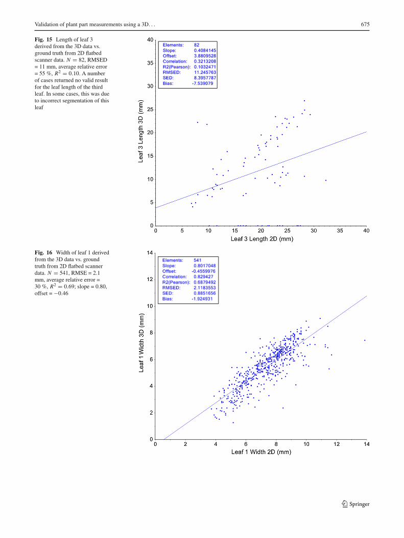
leaf length estimations as measured by the RMSED is 4.3and 3.6 mm for both leafs, and the average relative error is18 and 16 %. Unfortunately, the results for the third leaf arenot very good, as can be seen in Fig. 15 (correlation of 0.32,RMSED of 11, and average relative error of 55 %). Not onlythe spread is much larger, but there is a large number (16)of seedlings where the method gives no result (length = 0).Investigation shows that this is caused by a failure to cor-rectly segment the leaf. The third leaf usually is the first true

leaf, which is more lobed than the cotyledons. In the first stepof the segmentation method, the different lobes are often dif-ferent segments. These are then merged in the second step.However, this sometimes fails, resulting in a small segment.If the length of such a segment is below a threshold of 3 mm<3.1>, the method returns 0.

4.3 Leaf width

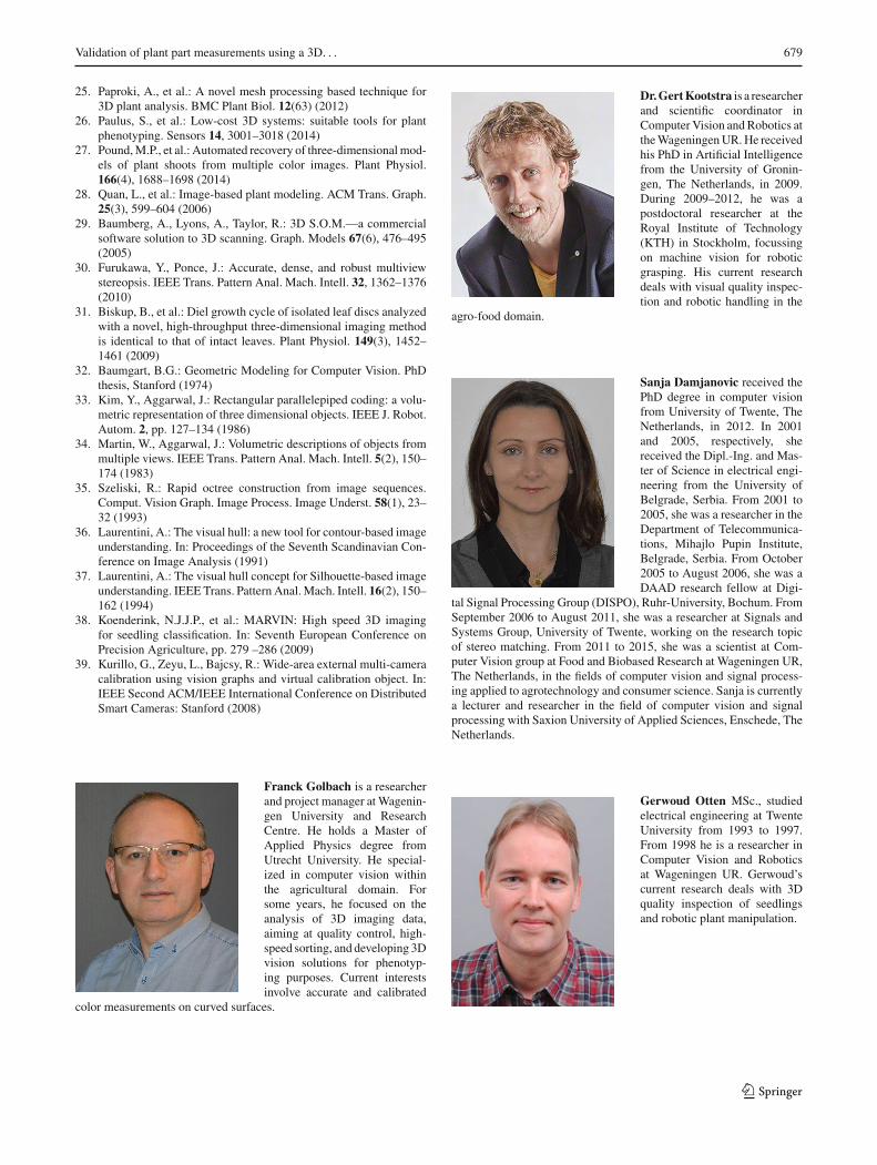
<2.3> Leaf width was measured using the proceduredescribed in Sect. 2.3.2. Results for leafs 1 and 2 are shownin Figs. 16 and 17:

The correlation of ourmethodwith the ground truth resultsis 0.83 for leaf 1 and 0.85 for leaf 2, with a RMSED ofrespectively 2.1 and 1.9 mm, and average relative error of 30and 27 %. These errors are smaller than for the length of theleafs, but since the width of the leafs is about one-third ofthe length, the relative error is larger. This may not come asa surprise; the number of voxels in this direction is less, andhence, the accuracy.

4.4 Leaf area

Leaf area is based on the method described in Sect. 2.3.3.Results are shown in Figs. 18 and 19. The method has acorrelation of 0.85, RMSED of 27, and average relative errorof 22 % for the first leaf and correlation of 0.88, RMSED of24, and average relative error of 19 % for the second leaf.

123


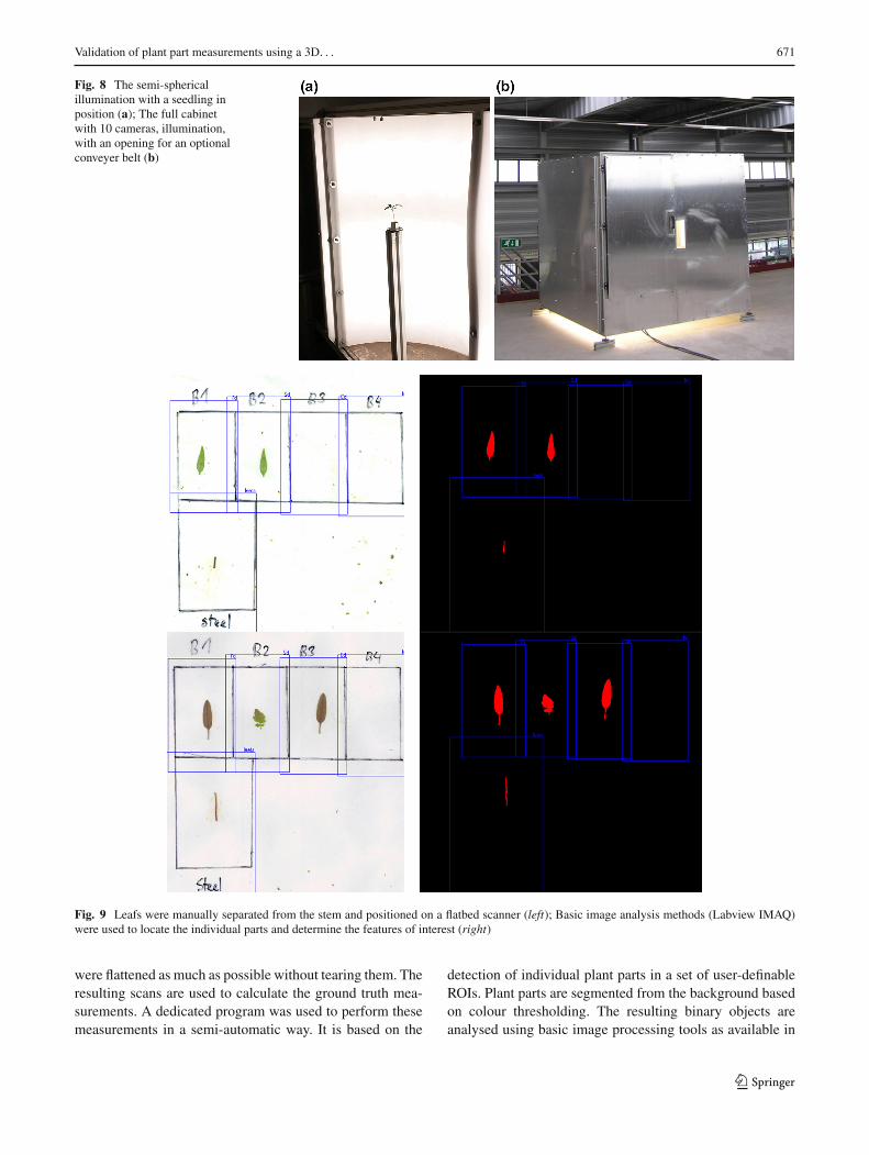
Fig. 13 Length of leaf 1derived from the 3D data vs.ground truth from 2D flatbedscanner data. N = 541, RMSED= 4.3 mm, average relative error= 18 % R2 = 0.83; slope = 0.89,offset = −1.25

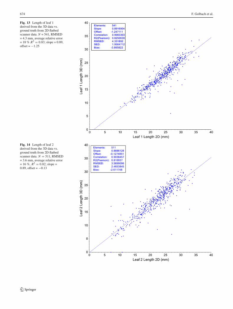
Fig. 14 Length of leaf 2derived from the 3D data vs.ground truth from 2D flatbedscanner data. N = 511, RMSED= 3.6 mm, average relative error= 16 %, R2 = 0.82; slope =0.89, offset = −0.13

123


Fig. 15 Length of leaf 3derived from the 3D data vs.ground truth from 2D flatbedscanner data. N = 82, RMSED= 11 mm, average relative error= 55 %, R2 = 0.10. A numberof cases returned no valid resultfor the leaf length of the thirdleaf. In some cases, this was dueto incorrect segmentation of thisleaf

Fig. 16 Width of leaf 1 derivedfrom the 3D data vs. groundtruth from 2D flatbed scannerdata. N = 541, RMSE = 2.1mm, average relative error =30 %, R2 = 0.69; slope = 0.80,offset = −0.46

123


Fig. 17 Width of leaf 2 derivedfrom the 3D data vs. groundtruth from 2D flatbed scannerdata. N = 541, RMSE = 1.9mm, average relative error =27 %, R2 = 0.73; slope = 0.96,offset = −1.44

Fig. 18 Area of leaf 1 derivedfrom the 3D data vs. groundtruth from 2D flatbed scannerdata. N = 541, RMSE = 28mm2, average relative error =22 % R2 = 0.72; slope = 1.05,offset = −14.8

123


Fig. 19 Area of leaf 2 derivedfrom the 3D data vs. groundtruth from 2D flatbed scannerdata. N = 511, RMSE = 24mm2, average relative error =19 %, R2 = 0.78; slope = 1.00,offset = −10.9

5 Discussion

In this paper, we presented methods to measure specific fea-tures of a seedling based on a 3D reconstruction of the plant.Implemented features include length, width and area of indi-vidual leafs, and length of the stem. These are some of thebasis phenotypic properties of a plant. The proposed methodis optimized for speed, to be used in high-throughput pheno-typing systems. The 3D reconstruction of the plant is createdusing a shape-from-silhouettemethod.The resulting3Dplantmodel is segmented in stem and leaf parts, from which stemand leaf parameters are calculated. Stem length, leaf length,and area can be determined with an average relative error ofapprox. 20 %; the error measuring the width of the leafs isclose to 30 %.

A clear benefit of the proposed method is its fast process-ing time. Other existingmethods for plant phenotyping usingfull 3D reconstruction from camera image are based onmore complex 3D reconstruction methods, such as multi-view stereo [27], structure-from-motion [28], space carving[25] or using laser-line scan devices [26]. These methodsare more accurate, but with the cost of very long process-ing times, making them not applicable for high-throughputphenotyping (<1 s). We put much effort in optimizing thespeed of our 3D reconstruction algorithm, which now runsin 20–60 ms, depending on the complexity of the plant, witha voxel space of 240×240×300 voxels and using 10 cameraswith a resolution of 1280 × 960 on a PC with a 3.2 GHz i7

processor. Other steps in our algorithm (stem/leaf segmenta-tion and the calculation of stem and leaf parameters) have notyet been optimized for speed. Calculation of stem and leafparameters has low complexity and is fast (25–60ms), but theimplementation of the stem/leaf segmentation is slow, taking100–200mswith incidental peaks up to 1000ms. Dependingon the structure of the leafs, the method’s first step can resultin many small segments, which then need to be merged ina second step. Moreover, the method has been implementedinefficiently in Labview.We are confident that we can greatlyimprove processing time with a more efficient implementa-tion and adapting the method to better deal with irregularlyshaped leafs.

To facilitate high-throughput plant phenotyping,wedevel-oped fast, relatively simple methods that approximate therelevant stem and leaf parameters. The leaf length is approx-imated by two line segments, which is an underestimationof the true length measured along the curved surface. Thisis reflected in Figs. 13 and 14 where the slope of the corre-lation between the 2D and 3D measurements is less than 1.Similarly, the leaf width is estimated by taking the Euclidiandistance between two points instead of following the actualsurface. Again, this results in an underestimation which canbe noticed in Figs. 16 and 17. Finally, themethod for measur-ing the leaf area assumes amainly horizontally (or vertically)oriented leaf with an underestimation of the area when theleaf is tilted. Despite these limitations, we believe that theresults of our system are very promising.

123


The camera setup has been developed such that fromeach camera perspective, the plant has a clear illuminatedbackground, which assures robust foreground/backgroundsegmentation. We do not use a top view, avoiding the typi-cal image-segmentation issues caused by pot, soil, moss andother clutter visible in the images.

We hope to further improve the results in the near future.First, the results show some limitations in the process ofstem and leaf segmentation. In case of very fine structures,the method does not always find the optimal position ofstem–leaf transition. We expect to improve this by apply-ing a skeletisation algorithm to the seedling, which will giveus a more accurate description of the plant connectivity andtopology. This will not only allow us to do a better segmenta-tion, but also to improve the measurements of, for instance,stem length. Next, to improve leaf measurements, we willdescribe the leaf by a fitted surface curved in 3D. Doing sowill not only increase the accuracy of the leaf measurements,but also reduce the sensitivity to noise. Itwill furthermore addthe possibility of measuring new features, like the shape ofthe leaf’s contour. Finally, we are working on a way of mod-elling more complex plants. One of the major challenges isthe way to deal with apparent loops in the model, i.e. sit-uations where it is not clear whether plant parts are reallyconnected, or just touching each other. To solve such ambi-guities, we will incorporate expert knowledge in the system,so that the most likely representation can be found.

For phenotyping purposes, improving accuracy is not theonly important issue. The ability to measure characteristicsof individual plant parts is also a promising advantage of a3D-based system. We hope that the system presented herecan contribute to this demand.

Acknowledgments The research leading to these results has receivedfunding from theEuropeanUnion’s Seventh Framework Programme forresearch, technological development and demonstration, in the Euro-pean Plant Phenotyping Network (EPPN), under Grant agreement no.284443. We would like to thank Bayer CropScience and Enza Zadenfor supplying the seedlings.

Open Access This article is distributed under the terms of the CreativeCommons Attribution 4.0 International License (http://creativecommons.org/licenses/by/4.0/), which permits unrestricted use, distribution,and reproduction in any medium, provided you give appropriate creditto the original author(s) and the source, provide a link to the CreativeCommons license, and indicate if changes were made.

References

1. Furbank, R.T., Tester, M.: Phenomics—technologies to relieve thephenotyping bottleneck. Trends Plant Sci. 16(12), 635–644 (2011)

2. Kolukisaoglu, Ü., Thurow, K.: Future and frontiers of automatedscreening in plant sciences. Plant Sci. 178(6), 476–484 (2010)

3. Fiorani, F., Schurr, U.: Future scenarios for plant phenotyping.Annu. Rev. Plant Biol. 64, 267–291 (2013)

4. Li, L., Zhang, Q., Huang, D.: A review of imaging techniques forplant phenotyping. Sensors 14(11), 20078–20111 (2014)

5. Rousseau, D., et al.: Multiscale imaging of plants: currentapproaches and challenges. Plant Methods 11(1), 6 (2015)

6. Bergstrasser, S., et al.: HyperART: non-invasive quantification ofleaf traits using hyperspectral absorption-reflectance-transmittanceimaging. Plant Methods 11(1), 1 (2015)

7. Biskup, B., et al.: A stereo imaging system for measuring structuralparameters of plant canopies. Plant Cell Environ. 30(10), 1299–1308 (2007)

8. van der Heijden, G., et al.: SPICY: towards automated phenotypingof large pepper plants in the greenhouse. Funct. Plant Biol. 39, 870–877 (2012)

9. Eberius, M., Lima-Guerra, J.: High-throughput plantphenotyping—data acquisition, transformation, and analy-sis. In: Bioinformatics: Tools and Applications, pp. 259–278.Springer, New York (2009)

10. Golzarian, M., et al.: Accurate inference of shoot biomass fromhigh-throughput images of cereal plants. Plant Methods 7(1), 2(2011)

11. Imaging robots. http://www.psb.ugent.be/infrastructure/391-image-robots

12. Granier, C., et al.: PHENOPSIS, an automated platform for repro-ducible phenotyping of plant responses to soil water deficit inArabidopsis thaliana permitted the identification of an accessionwith low sensitivity to soil water deficit. New Phytol. 169(3), 623–635 (2006)

13. Hartmann,A., et al.: HTPheno: an image analysis pipeline for high-throughput plant phenotyping. BMC Bioinf. 12(148), 1–9 (2011)

14. Jansen, M., et al.: Simultaneous phenotyping of leaf growth andchlorophyll fluorescence via GROWSCREEN FLUORO allowsdetection of stress tolerance in Arabidopsis thaliana and otherrosette plants. Funct. Plant Biol. 36(11), 902–914 (2009)

15. Walter, A., et al.: Dynamics of seedling growth acclimation towardsaltered light conditions can be quantified via GROWSCREEN: asetup and procedure designed for rapid optical phenotyping of dif-ferent plant species. New Phytol. 174(2), 447–455 (2007)

16. Tisné, S., et al.: Phenoscope: an automated large-scale phenotypingplatform offering high spatial homogeneity. Plant J. 74(3), 534–44(2013)

17. Subramanian, R., Spalding, E., Ferrier, N.: A high throughput robotsystem for machine vision based plant phenotype studies. Mach.Vision Appl. 24(3), 619–636 (2013)

18. Minervini, M., Abdelsamea, M.M., Tsaftaris, S.A.: Image-basedplant phenotyping with incremental learning and active contours.Ecol. Inf. 23 (2014)

19. Pereyra-Irujo, G.A., et al.: GlyPh: a low-cost platform for pheno-typing plant growth and water use. Funct. Plant Biol. 39, 905–913(2012)

20. Dornbusch, T., et al.: Measuring the diurnal pattern of leafhyponasty and growth in Arabidopsis—a novel phenotypingapproach using laser scanning. Funct. Plant Biol. 39, 860–869(2012)

21. Alenya, G., Dellen, B., Torras, C.: 3D modelling of leaves fromcolor and ToF data for robotized plant measuring. In: 2011 IEEEInternational Conference on Robotics and Automation (ICRA)(2011)

22. Chéné, Y., et al.: On the use of depth camera for 3D phenotypingof entire plants. Comput. Electron. Agric. 82, 122–127 (2012)

23. Klose, R., Penlington, J., Ruckelshausen, A.: Usability study of 3Dtime-of-flight cameras for automatic plant phenotyping. BornimerAgrartechnische Berichte 69, 93–105 (2009)

24. Andersen, H.J., Reng, L., Kirk, K.: Geometric plant properties byrelaxed stereo vision using simulated annealing. Comput. Electron.Agric. 49, 219–232 (2005)

123

http://creativecommons.org/licenses/by/4.0/

http://creativecommons.org/licenses/by/4.0/

http://www.psb.ugent.be/infrastructure/391-image-robots

http://www.psb.ugent.be/infrastructure/391-image-robots


25. Paproki, A., et al.: A novel mesh processing based technique for3D plant analysis. BMC Plant Biol. 12(63) (2012)

26. Paulus, S., et al.: Low-cost 3D systems: suitable tools for plantphenotyping. Sensors 14, 3001–3018 (2014)

27. Pound,M.P., et al.: Automated recovery of three-dimensionalmod-els of plant shoots from multiple color images. Plant Physiol.166(4), 1688–1698 (2014)

28. Quan, L., et al.: Image-based plant modeling. ACM Trans. Graph.25(3), 599–604 (2006)

29. Baumberg, A., Lyons, A., Taylor, R.: 3D S.O.M.—a commercialsoftware solution to 3D scanning. Graph. Models 67(6), 476–495(2005)

30. Furukawa, Y., Ponce, J.: Accurate, dense, and robust multiviewstereopsis. IEEE Trans. Pattern Anal. Mach. Intell. 32, 1362–1376(2010)

31. Biskup, B., et al.: Diel growth cycle of isolated leaf discs analyzedwith a novel, high-throughput three-dimensional imaging methodis identical to that of intact leaves. Plant Physiol. 149(3), 1452–1461 (2009)

32. Baumgart, B.G.: Geometric Modeling for Computer Vision. PhDthesis, Stanford (1974)

33. Kim, Y., Aggarwal, J.: Rectangular parallelepiped coding: a volu-metric representation of three dimensional objects. IEEE J. Robot.Autom. 2, pp. 127–134 (1986)

34. Martin, W., Aggarwal, J.: Volumetric descriptions of objects frommultiple views. IEEE Trans. Pattern Anal. Mach. Intell. 5(2), 150–174 (1983)

35. Szeliski, R.: Rapid octree construction from image sequences.Comput. Vision Graph. Image Process. Image Underst. 58(1), 23–32 (1993)

36. Laurentini, A.: The visual hull: a new tool for contour-based imageunderstanding. In: Proceedings of the Seventh Scandinavian Con-ference on Image Analysis (1991)

37. Laurentini, A.: The visual hull concept for Silhouette-based imageunderstanding. IEEETrans. Pattern Anal.Mach. Intell. 16(2), 150–162 (1994)

38. Koenderink, N.J.J.P., et al.: MARVIN: High speed 3D imagingfor seedling classification. In: Seventh European Conference onPrecision Agriculture, pp. 279 –286 (2009)

39. Kurillo, G., Zeyu, L., Bajcsy, R.: Wide-area external multi-cameracalibration using vision graphs and virtual calibration object. In:IEEE Second ACM/IEEE International Conference on DistributedSmart Cameras: Stanford (2008)

Franck Golbach is a researcherand project manager atWagenin-gen University and ResearchCentre. He holds a Master ofApplied Physics degree fromUtrecht University. He special-ized in computer vision withinthe agricultural domain. Forsome years, he focused on theanalysis of 3D imaging data,aiming at quality control, high-speed sorting, and developing 3Dvision solutions for phenotyp-ing purposes. Current interestsinvolve accurate and calibrated

color measurements on curved surfaces.

Dr.GertKootstra is a researcherand scientific coordinator inComputer Vision andRobotics attheWageningenUR.He receivedhis PhD in Artificial Intelligencefrom the University of Gronin-gen, The Netherlands, in 2009.During 2009–2012, he was apostdoctoral researcher at theRoyal Institute of Technology(KTH) in Stockholm, focussingon machine vision for roboticgrasping. His current researchdeals with visual quality inspec-tion and robotic handling in the

agro-food domain.

Sanja Damjanovic received thePhD degree in computer visionfrom University of Twente, TheNetherlands, in 2012. In 2001and 2005, respectively, shereceived the Dipl.-Ing. and Mas-ter of Science in electrical engi-neering from the University ofBelgrade, Serbia. From 2001 to2005, she was a researcher in theDepartment of Telecommunica-tions, Mihajlo Pupin Institute,Belgrade, Serbia. From October2005 to August 2006, she was aDAAD research fellow at Digi-

tal Signal Processing Group (DISPO), Ruhr-University, Bochum. FromSeptember 2006 to August 2011, she was a researcher at Signals andSystems Group, University of Twente, working on the research topicof stereo matching. From 2011 to 2015, she was a scientist at Com-puter Vision group at Food and Biobased Research at Wageningen UR,The Netherlands, in the fields of computer vision and signal process-ing applied to agrotechnology and consumer science. Sanja is currentlya lecturer and researcher in the field of computer vision and signalprocessing with Saxion University of Applied Sciences, Enschede, TheNetherlands.

Gerwoud Otten MSc., studiedelectrical engineering at TwenteUniversity from 1993 to 1997.From 1998 he is a researcher inComputer Vision and Roboticsat Wageningen UR. Gerwoud’scurrent research deals with 3Dquality inspection of seedlingsand robotic plant manipulation.

123


Rick van de Zedde is a seniorresearcher/ business developerfor Computer Vision at theWageningen UR Food &Biobased Research Institute inthe Netherlands, where he hasworked since 2004. His back-ground is in Artificial Intelli-gence with a focus on imagingand robotics. In 2002 he grad-uated with an MSc in ArtificialIntelligence from the Universityof Groningen. Since 2006 he hasbeen a coordinator of GreenVi-sion, the centre of expertise for

image processing in the agrofood industry (http://greenvision.wur.nl).

123

http://greenvision.wur.nl

Documents

Validation of plant part measurements using a 3D