Embed Size (px)
Citation preview

123
S P R I N G E R B R I E F S I NP E T R O L E U M G E O S C I E N C E & E N G I N E E R I N G
Vahid Tavakoli
Carbonate Reservoir Heterogeneity
Overcoming the Challenges

SpringerBriefs in Petroleum Geoscience &Engineering
Series Editors
Dorrik Stow, Institute of Petroleum Engineering, Heriot-Watt University,Edinburgh, UKMark Bentley, AGR TRACS International Ltd, Aberdeen, UKJebraeel Gholinezhad, School of Engineering, University of Portsmouth,Portsmouth, UKLateef Akanji, Petroleum Engineering, University of Aberdeen, Aberdeen, UKKhalik Mohamad Sabil, School of Energy, Geoscience, Infrastructure and Society,Heriot-Watt University, Edinburgh, UKSusan Agar, Oil & Energy, Aramco Research Center, Houston, USAKenichi Soga, Department of Civil and Environmental Engineering, University ofCalifornia, Berkeley, USAA. A. Sulaimon, Department of Petroleum Engineering, Universiti TeknologiPETRONAS, Seri Iskandar, Malaysia

The SpringerBriefs series in Petroleum Geoscience & Engineering promotes andexpedites the dissemination of substantive new research results, state-of-the-artsubject reviews and tutorial overviews in the field of petroleum exploration,petroleum engineering and production technology. The subject focus is on upstreamexploration and production, subsurface geoscience and engineering. These concisesummaries (50–125 pages) will include cutting-edge research, analytical methods,advanced modelling techniques and practical applications. Coverage will extend toall theoretical and applied aspects of the field, including traditional drilling,shale-gas fracking, deepwater sedimentology, seismic exploration, pore-flowmodelling and petroleum economics. Topics include but are not limited to:
• Petroleum Geology & Geophysics• Exploration: Conventional and Unconventional• Seismic Interpretation• Formation Evaluation (well logging)• Drilling and Completion• Hydraulic Fracturing• Geomechanics• Reservoir Simulation and Modelling• Flow in Porous Media: from nano- to field-scale• Reservoir Engineering• Production Engineering• Well Engineering; Design, Decommissioning and Abandonment• Petroleum Systems; Instrumentation and Control• Flow Assurance, Mineral Scale & Hydrates• Reservoir and Well Intervention• Reservoir Stimulation• Oilfield Chemistry• Risk and Uncertainty• Petroleum Economics and Energy Policy
Contributions to the series can be made by submitting a proposal to the responsibleSpringer contact, Charlotte Cross at [email protected] or the AcademicSeries Editor, Prof Dorrik Stow at [email protected].
More information about this series at http://www.springer.com/series/15391

Vahid Tavakoli
Carbonate ReservoirHeterogeneityOvercoming the Challenges
123

Vahid TavakoliSchool of Geology, College of ScienceUniversity of TehranTehran, Iran
ISSN 2509-3126 ISSN 2509-3134 (electronic)SpringerBriefs in Petroleum Geoscience & EngineeringISBN 978-3-030-34772-7 ISBN 978-3-030-34773-4 (eBook)https://doi.org/10.1007/978-3-030-34773-4
© The Author(s), under exclusive license to Springer Nature Switzerland AG 2020This work is subject to copyright. All rights are solely and exclusively licensed by the Publisher, whetherthe whole or part of the material is concerned, specifically the rights of translation, reprinting, reuse ofillustrations, recitation, broadcasting, reproduction on microfilms or in any other physical way, andtransmission or information storage and retrieval, electronic adaptation, computer software, or by similaror dissimilar methodology now known or hereafter developed.The use of general descriptive names, registered names, trademarks, service marks, etc. in thispublication does not imply, even in the absence of a specific statement, that such names are exempt fromthe relevant protective laws and regulations and therefore free for general use.The publisher, the authors and the editors are safe to assume that the advice and information in thisbook are believed to be true and accurate at the date of publication. Neither the publisher nor theauthors or the editors give a warranty, expressed or implied, with respect to the material containedherein or for any errors or omissions that may have been made. The publisher remains neutral with regardto jurisdictional claims in published maps and institutional affiliations.
This Springer imprint is published by the registered company Springer Nature Switzerland AGThe registered company address is: Gewerbestrasse 11, 6330 Cham, Switzerland
Preface
Heterogeneity is an intrinsic property of all carbonate reservoirs. The propertiesof these reservoirs considerably change both laterally and vertically. Lateralchanges are usually the result of various depositional settings, while verticalheterogeneities are caused by basin evolution through time. Available data fromthese reservoirs are very limited and so predicting the distribution of propertiesbetween the wells is very complicated. The hydrocarbon in place is calculated usingthese predictions and so they are very important. In fact, many aspects of thereservoir studies are about heterogeneities. Facies analysis and classifications,determining sedimentary environments, reservoir rock typing, flow unit determi-nation and sequence stratigraphy are some examples.
Despite this importance, few studies have been published about the hetero-geneity of the carbonate reservoirs. How the heterogeneity of a reservoir is eval-uated? Where we should start and how the process continues? How the variousscales of heterogeneity are related to each other? This book tries to answer thesequestions. It starts with an introduction about the heterogeneity and states theproblem. The term is defined, and the importance of its study is explained. Then, itscauses are considered, and the required materials are discussed. Chapter 1 ends withthe scales of heterogeneity which are one of the most important aspects of thisconcept. This book has been organized based on the scale of heterogeneity frommicro- to macroscale. Each chapter is divided into two parts. At first, the problem isdiscussed, and then, the solution is considered. In Chap. 2, facies analysis, diage-netic impacts on the reservoir, porosity–permeability relationships and pore throatsizes are considered, and then, pore system classifications, rock typing and elec-trofacies are introduced to overcome the challenge of heterogeneity in microscale.Chapter 3 is about the heterogeneities in mesoscale. Sedimentary environments aredefined to organize the homogenous facies in a larger body. Hydraulic flow units,cyclicities and stratigraphic correlations are discussed for the same reason. Inmacroscopic scale which is the subject of Chap. 4, larger-scale variables such asseismic data and interpretations, fracturing, stratifications, sequence stratigraphic
v

concepts and maps are discussed. This book ends with the petrophysical evaluationsand how the analyst can overcome the challenges of heterogeneities in thesecalculations.
I am thankful to my beloved wife, Dr. M. Naderi-Khujin, for designing mostfigures of this book. Her abilities in illustrating the most complicated concepts withsome simple but beautiful figures are endless. Our personal communications alsohelped me a lot, especially on macroscopic heterogeneities. I want to thank mycolleague Dr. H. Rahimpour-Bonab for giving me brilliant ideas about differentaspects of reservoir heterogeneity. I also appreciate the cooperation of my Ph.D.student A. Jamalian for illustrating some figures and helping me in organizing someparts of this book. The preparation of this book was made possible through the helpof my M.S. students, M. Nazemi, M. H. Nazari, A. Mondak and B. Meidani. Lastbut not least, I want to thank all of my colleagues and students at the University ofTehran which are really trying to develop the science of geology in any way thatthey can. Please let me know any idea, critique or suggestion which you probablyhave about this book.
Tehran, Iran Vahid TavakoliSeptember 2019
vi Preface

Contents
1 Reservoir Heterogeneity: An Introduction . . . . . . . . . . . . . . . . . . . . 11.1 Definition . . . . . . . . . . . . . . . . . . . . . . . . . . . . . . . . . . . . . . . . . 1
1.1.1 Related Scientific Definitions . . . . . . . . . . . . . . . . . . . . . 51.2 Why It Is Important? . . . . . . . . . . . . . . . . . . . . . . . . . . . . . . . . 81.3 Sources of Heterogeneity . . . . . . . . . . . . . . . . . . . . . . . . . . . . . 101.4 Materials . . . . . . . . . . . . . . . . . . . . . . . . . . . . . . . . . . . . . . . . . 111.5 Heterogeneity Scales . . . . . . . . . . . . . . . . . . . . . . . . . . . . . . . . . 12References . . . . . . . . . . . . . . . . . . . . . . . . . . . . . . . . . . . . . . . . . . . . . 15
2 Microscopic Heterogeneity . . . . . . . . . . . . . . . . . . . . . . . . . . . . . . . . 172.1 Facies Analysis . . . . . . . . . . . . . . . . . . . . . . . . . . . . . . . . . . . . . 172.2 Diagenetic Impacts . . . . . . . . . . . . . . . . . . . . . . . . . . . . . . . . . . 20
2.2.1 Limestones . . . . . . . . . . . . . . . . . . . . . . . . . . . . . . . . . . 212.2.2 Dolomitic Reservoirs . . . . . . . . . . . . . . . . . . . . . . . . . . . 232.2.3 Diagenetic Facies . . . . . . . . . . . . . . . . . . . . . . . . . . . . . . 252.2.4 Quantitative Diagenesis . . . . . . . . . . . . . . . . . . . . . . . . . 26
2.3 CT Scan Data . . . . . . . . . . . . . . . . . . . . . . . . . . . . . . . . . . . . . . 302.4 Porosity–Permeability Relationships . . . . . . . . . . . . . . . . . . . . . . 31
2.4.1 Limestones . . . . . . . . . . . . . . . . . . . . . . . . . . . . . . . . . . 322.4.2 Dolomites . . . . . . . . . . . . . . . . . . . . . . . . . . . . . . . . . . . 33
2.5 Pore Throat Sizes . . . . . . . . . . . . . . . . . . . . . . . . . . . . . . . . . . . 362.6 Sedimentary Structures . . . . . . . . . . . . . . . . . . . . . . . . . . . . . . . 372.7 Pore System Classifications . . . . . . . . . . . . . . . . . . . . . . . . . . . . 392.8 Rock Typing . . . . . . . . . . . . . . . . . . . . . . . . . . . . . . . . . . . . . . 462.9 Electrofacies . . . . . . . . . . . . . . . . . . . . . . . . . . . . . . . . . . . . . . . 472.10 Microscopic Uncertainties . . . . . . . . . . . . . . . . . . . . . . . . . . . . . 47References . . . . . . . . . . . . . . . . . . . . . . . . . . . . . . . . . . . . . . . . . . . . . 48
vii
3 Mesoscopic Heterogeneity . . . . . . . . . . . . . . . . . . . . . . . . . . . . . . . . . 533.1 Sedimentary Environments . . . . . . . . . . . . . . . . . . . . . . . . . . . . 533.2 Hydraulic Flow Units . . . . . . . . . . . . . . . . . . . . . . . . . . . . . . . . 563.3 Cyclicity . . . . . . . . . . . . . . . . . . . . . . . . . . . . . . . . . . . . . . . . . 583.4 Upscaling . . . . . . . . . . . . . . . . . . . . . . . . . . . . . . . . . . . . . . . . . 613.5 Stratigraphic Correlation . . . . . . . . . . . . . . . . . . . . . . . . . . . . . . 63References . . . . . . . . . . . . . . . . . . . . . . . . . . . . . . . . . . . . . . . . . . . . . 65
4 Macroscopic Heterogeneity . . . . . . . . . . . . . . . . . . . . . . . . . . . . . . . . 694.1 Seismic Interpretation . . . . . . . . . . . . . . . . . . . . . . . . . . . . . . . . 704.2 Fracturing . . . . . . . . . . . . . . . . . . . . . . . . . . . . . . . . . . . . . . . . . 724.3 Stratification . . . . . . . . . . . . . . . . . . . . . . . . . . . . . . . . . . . . . . . 764.4 Sequence Stratigraphy . . . . . . . . . . . . . . . . . . . . . . . . . . . . . . . . 774.5 Reservoir Compartmentalization . . . . . . . . . . . . . . . . . . . . . . . . 804.6 Reservoir Zonation . . . . . . . . . . . . . . . . . . . . . . . . . . . . . . . . . . 834.7 Maps . . . . . . . . . . . . . . . . . . . . . . . . . . . . . . . . . . . . . . . . . . . . 854.8 Reservoir Tomography . . . . . . . . . . . . . . . . . . . . . . . . . . . . . . . 904.9 Macroscopic Uncertainties . . . . . . . . . . . . . . . . . . . . . . . . . . . . . 93References . . . . . . . . . . . . . . . . . . . . . . . . . . . . . . . . . . . . . . . . . . . . . 93
5 Petrophysical Evaluations . . . . . . . . . . . . . . . . . . . . . . . . . . . . . . . . . 975.1 Effects of Heterogeneity . . . . . . . . . . . . . . . . . . . . . . . . . . . . . . 975.2 Selecting the Parameters . . . . . . . . . . . . . . . . . . . . . . . . . . . . . . 1025.3 Solving the Problem . . . . . . . . . . . . . . . . . . . . . . . . . . . . . . . . . 106References . . . . . . . . . . . . . . . . . . . . . . . . . . . . . . . . . . . . . . . . . . . . . 108
viii Contents
Chapter 1Reservoir Heterogeneity:An Introduction
Abstract The ultimate goal of reservoir studies is predicting the properties andtheir controlling factors in a reservoir body based on limited data mainly from bore-holes. Reservoir heterogeneity means variations of reservoir properties in space andtime, and so this concept is the most important factor in reservoir studies. Despitesuch importance, relatively few works have been focused or documented differentaspects of this subject. Evaluating heterogeneity is more complicated in carbonateswhich have diverse facies and are more prone to diagenetic processes. Textures andallochems vary considerably at small scales of carbonate reservoirs. Different faciesare deposited in various depositional environments. They also change in response tosea-level changes and climate conditions. These building blocks integrate to createvarious facies belts and geometries of the depositional settings. These geometriesare used for propagation of reservoir properties in field scale. Diagenetic processesmodify these properties. They follow the primary textural characteristics in manycases, especially in early diagenesis. Anyway, many late diagenetic processes, suchas fractures, crosscut the primary facies as well as other diagenetic features. Whilefacies variations create heterogeneity at larger scales, diagenesis is responsible forchanges at smaller scales.
Heterogeneities are present in microscopic, mesoscopic, macroscopic and megas-copic scales. Facies and pore types are examples of microscopic variations, whilesedimentary structures, stratification and reservoir compartmentalization are con-sidered as large-scale heterogeneities. They can be studied using various tools andmethods from thin sections to core CT scanning, core description, reservoir zonation,correlations, maps and seismic sections.
1.1 Definition
In the simplest approach, heterogeneitymeans diversity in properties in a single body.The terms variability, discrepancy, randomness, complexity, diversity and deviation
© The Author(s), under exclusive license to Springer Nature Switzerland AG 2020V. Tavakoli, Carbonate Reservoir Heterogeneity,SpringerBriefs in Petroleum Geoscience & Engineering,https://doi.org/10.1007/978-3-030-34773-4_1
1
2 1 Reservoir Heterogeneity: An Introduction
from a norm could be compared with this concept. In reservoir studies, the proper-ties of interest are fluid flow and storage-related characteristics. All reservoir-relatedvariabilities are included in this concept. Common examples include mineralogy,absolute and relative permeability, pore types, pore volume, pore throat size dis-tribution, textural properties such as grain size and sorting, diagenetic processessuch as cementation and dissolution and the production rate. Some authors (Li andReynolds 1995; Zhengquan et al. 1997) believe that the change in property in three-dimensional space causes system heterogeneity, while others (e.g., Fitch et al. 2015)add the time concept to the definition. They stated that changing a property over timealso increases the heterogeneity of a system. Change in discrete object density inspace was also defined as heterogeneity (Frazer et al. 2005).
The heterogeneity of a sample or volume strongly depends on the property ofinterest. These properties could be dependent on or independent from each other.For example, one meter of reservoir core in well scale could be homogeneous fromporosity frequency distribution point of view, while it is heterogeneous when poretypes are considered. Permeability distribution in this core may be dependent onor independent from porosity. For uniform interparticle porosities, for example, itdepends on porosity, but in the case of various pore types, it is mainly independentfrom pore volume.
Based on previous literatures, Fitch and his co-workers (2015) defined hetero-geneity as the change in one or a combination of some various parameters in spaceand/or time which strongly depends on desired scale. They correctly point to theconcept of a combination of parameters which determines the reservoir quality vari-ation in space and time. For many years, researchers tried to define a unique unitwhich includes all of these properties. The term rock type is commonly used forthis purpose. Although various methods have been introduced so far (such as geo-logical rock typing (GRT) (Tavakoli 2018), reservoir quality index (RQI) and flowzone indicator (FZI) (Amaefule et al. 1993), Winland R35 method (Kolodzie 1980),Lucia rock fabric number (RFN) (Lucia and Conti 1987; Lucia 1995), none of thesemethods can be applied in all cases. It means that more research is necessary in thisfield.
Weber (1986) defined heterogeneity as non-uniformvariations of reservoir param-eters such as porosity, permeability and pore types in space. He believed that theheterogeneity of a reservoir is initially caused by primary depositional characteris-tics (facies), followed by diagenetic processes after deposition. This is true becauseall reservoir properties are the result of these two processes. The cause of variousmanifestations on reservoir heterogeneity is different studied scales. This will bediscussed in Sect. 1.5.
It should be mentioned that heterogeneity and homogeneity are two ends of acontinuous spectrum. This means that the heterogeneity of two systems can be com-pared and the systems may be more or less heterogeneous. Increasing heterogeneitymeans increase in the random mixing of the interested parameter (Fitch et al. 2015).So, there are hierarchies in heterogeneity of a reservoir. Key classes and ranges are
1.1 Definition 3
defined to break these continuous scales and enable us to compare various reser-voirs from this point of view. Examples are rock types, hydraulic flow units (HFU),sedimentary facies and even a system tract of a sequence.
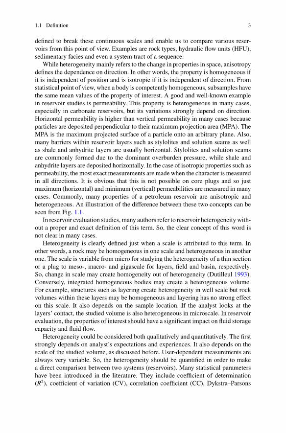
While heterogeneity mainly refers to the change in properties in space, anisotropydefines the dependence on direction. In other words, the property is homogeneous ifit is independent of position and is isotropic if it is independent of direction. Fromstatistical point of view, when a body is competently homogeneous, subsamples havethe same mean values of the property of interest. A good and well-known examplein reservoir studies is permeability. This property is heterogeneous in many cases,especially in carbonate reservoirs, but its variations strongly depend on direction.Horizontal permeability is higher than vertical permeability in many cases becauseparticles are deposited perpendicular to their maximum projection area (MPA). TheMPA is the maximum projected surface of a particle onto an arbitrary plane. Also,many barriers within reservoir layers such as stylolites and solution seams as wellas shale and anhydrite layers are usually horizontal. Stylolites and solution seamsare commonly formed due to the dominant overburden pressure, while shale andanhydrite layers are deposited horizontally. In the case of isotropic properties such aspermeability, the most exact measurements are made when the character is measuredin all directions. It is obvious that this is not possible on core plugs and so justmaximum (horizontal) and minimum (vertical) permeabilities are measured in manycases. Commonly, many properties of a petroleum reservoir are anisotropic andheterogeneous. An illustration of the difference between these two concepts can beseen from Fig. 1.1.
In reservoir evaluation studies, many authors refer to reservoir heterogeneitywith-out a proper and exact definition of this term. So, the clear concept of this word isnot clear in many cases.
Heterogeneity is clearly defined just when a scale is attributed to this term. Inother words, a rock may be homogeneous in one scale and heterogeneous in anotherone. The scale is variable from micro for studying the heterogeneity of a thin sectionor a plug to meso-, macro- and gigascale for layers, field and basin, respectively.So, change in scale may create homogeneity out of heterogeneity (Dutilleul 1993).Conversely, integrated homogeneous bodies may create a heterogeneous volume.For example, structures such as layering create heterogeneity in well scale but rockvolumes within these layers may be homogeneous and layering has no strong effecton this scale. It also depends on the sample location. If the analyst looks at thelayers’ contact, the studied volume is also heterogeneous in microscale. In reservoirevaluation, the properties of interest should have a significant impact on fluid storagecapacity and fluid flow.
Heterogeneity could be considered both qualitatively and quantitatively. The firststrongly depends on analyst’s expectations and experiences. It also depends on thescale of the studied volume, as discussed before. User-dependent measurements arealways very variable. So, the heterogeneity should be quantified in order to makea direct comparison between two systems (reservoirs). Many statistical parametershave been introduced in the literature. They include coefficient of determination(R2), coefficient of variation (CV), correlation coefficient (CC), Dykstra–Parsons

4 1 Reservoir Heterogeneity: An Introduction
Fig. 1.1 A schematic representation of heterogeneity versus anisotropy in tidal channels
coefficient, Lorenz plot and probability distribution function (PDF). The qualitativeanalysis can be tested with these parameters. For example, geological rock types(Tavakoli 2018) are determined based on the geologist’s experience with respect tothe depositional properties (facies) and diagenetic processes. The heterogeneity ofthe petrophysical properties (such as porosity and permeability) of these rock typescan be evaluated using the above-mentioned statistical methods. R2 between porosityand permeability and CV for many petrophysical variables within each rock type aresome examples (Nazemi et al. 2018 for example).
Quantifying reservoir heterogeneity is not a simple process. First of all, manyvariables are involved. Any single parameter is inadequate to properly evaluate thevariations of all reservoir characteristics in space and time. For example, many tex-tural (such as micrite content, allochems’ size, sorting, interparticle space) or dia-genetic parameters (such as dolomitization, dissolution, cementation, compaction)can change the reservoir properties. These parameters are strongly heterogeneousin many carbonate reservoirs. So, they should be included in any statistical calcula-tions. Other quantitative parameters such as porosity and permeability should alsobe involved. So, a unique unit should be defined to solve the problem. Defining suchunit also depends on the scale of interest. For example, hydraulic flow units and
1.1 Definition 5
electrofacies are homogeneous in microscopic scale, while a sequence stratigraphicunit is defined in field scale. This is discussed in Chaps. 2–4. The second problem islimitations in the number of samples. In many cases, there are not enough samplesto adequately address the variations in reservoir properties. The wells are generallyabout 8 inch (20 cm) in diameter in reservoir part. This is just a small part of thereservoir body. If we consider 1 km distance between two wells, the interwell spaceis about 5000 times larger than this volume of data! In fact, we are creating thisvolume just based on such limited data. There is a very interesting scientific storybehind this creation. This story is the subject of this book.
Many works have been focused on overcoming this challenge. In fact, we aremanaging the reservoir heterogeneity in many parts of a carbonate reservoir charac-terization. Some examples are defining depositional and diagenetic facies, reservoirrock typing, flow unit determination, upscaling, reservoir zonation and sequencestratigraphy.
1.1.1 Related Scientific Definitions
Evaluating the heterogeneity is a very important process in any carbonate reservoircharacterization. So, many researchers have attempted to introduce a scientific pro-cedure to define a homogeneous unit and classify the reservoir samples based ontheir heterogeneity. Readers are familiar with the results of some of these studies.For example, a microfacies defines carbonate samples with specific sedimentolog-ical and paleontological characteristics (Flugel 2010). It is obvious that this is aknown method to classify depositional properties of carbonate rocks based on theirenvironmental settings. The goal of such classification is interpreting the primarydepositional conditions. Regarding the heterogeneity of a carbonate reservoir, eachsample has its specific characteristics in petrographical studies and so there will benumerous names for them. Naming the samples based on Dunham (1962) classifi-cation combined with Folk (1959) prefixes for the allochems with more than 10%frequency is a good example. For grainstone samples with various amounts of bio-clasts and ooids, four different names could be present including ooid grainstone,bioclast grainstone, ooid bioclast grainstone and bioclast ooid grainstone. The pres-ence of another allochem such as intraclast, pellet, peloid or oncoid increases thisdiversity. Classifying these samples into variousmicrofacies solves the problem. Thisexample can be named bioclast/ooid grainstone and shows deposition in high-energyshola environment. Another familiar example is rock typing. Rock types are sampleswith similar reservoir properties (Tiab and Donaldson 2015; Tavakoli 2018). Thereare various methods for determining the rock types of a reservoir, from qualitativegeological point of view to quantitative approaches such as RQI/FZI, Lorenz andWinland method.
Some others have limited application in reservoir characterization. For example,Poeter and Gaylord (1990) defined the term “hydrofacies” as a three-dimensionalaquifer element in the study of Hanford site aquifer. They believed that if hydraulic
6 1 Reservoir Heterogeneity: An Introduction
properties-relateddata combinewith connection related characteristics, the resultwillbe a hydrofacies. They stated that such definition significantly improves the accuracyof the numericalmodels. The termused later in both aquifers andpetroleum reservoirsfor evaluating and managing the heterogeneity (such as Eaton 2006; Engdahl et al.2010; Bakshevskaya and Pozdnyakov 2013; Finkel et al. 2016; Hsieh et al. 2017;Bianchi and Pedretti 2018; Song et al. 2019). They introduced a new term for an oldconcept. In fact, the rock type has the same meaning in formation evaluation.
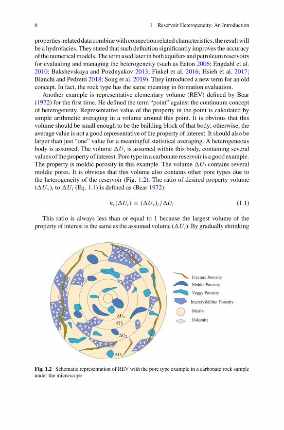
Another example is representative elementary volume (REV) defined by Bear(1972) for the first time. He defined the term “point” against the continuum conceptof heterogeneity. Representative value of the property in the point is calculated bysimple arithmetic averaging in a volume around this point. It is obvious that thisvolume should be small enough to be the building block of that body; otherwise, theaverage value is not a good representative of the property of interest. It should also belarger than just “one” value for a meaningful statistical averaging. A heterogeneousbody is assumed. The volume �Ui is assumed within this body, containing severalvalues of the property of interest. Pore type in a carbonate reservoir is a good example.The property is moldic porosity in this example. The volume �Ui contains severalmoldic pores. It is obvious that this volume also contains other pore types due tothe heterogeneity of the reservoir (Fig. 1.2). The ratio of desired property volume(�Uv)i to �Ui (Eq. 1.1) is defined as (Bear 1972):
ni (�Ui ) = (�Uv)i/�Ui (1.1)
This ratio is always less than or equal to 1 because the largest volume of theproperty of interest is the same as the assumed volume (�Ui). By gradually shrinking
Fig. 1.2 Schematic representation of REV with the pore type example in a carbonate rock sampleunder the microscope

1.1 Definition 7
Fig. 1.3 Quantitative definition of REV and the suitable size of a homogeneous sample
the size of �Ui, the fluctuations of �Ui versus ni(�Ui) decrease and a nearly flatplateau is formed, because theoretically there is a certain size for �Ui where thevolume is almost homogeneous (�U0). This size is scale-dependent and can bedefined for any property (Fig. 1.3). The volume of �Ui where the ni(�Ui) is nearlya constant value is REV of that property. After this limit, the ratio approaches zero or1 depends on the position of the property in the body. If the property is in the centerof the volume, the smallest volume will be completely filled and the value is 1. Incontrast, if the volume of the property inside the smallest �Ui is zero, the ratio willbe zero, too. As REV is a nearly homogeneous volume, a statistical average can beassigned to its center.
Many researchers have attempted to evaluate the potential of this method in reser-voir studies. Bachmat and Bear (1987) explained the concept from mathematicalpoint of view. Brown and his co-workers (2000) used REV for evaluation of the suit-able core sample size. Eaton (2006) explained that the REV is the smallest volumewith the same governing equations of flow. Nordahl and Ringrose (2008) applied themethod to permeability data in heterolithic deposits. Vik and his co-workers (2013)used the method for understanding the proper sample size to characterize a vuggycarbonate reservoir.
The REV is the smallest volume of a reservoir which average values of the prop-erties can be performed. So, it is very useful for selecting the smallest block for anumerical reservoir modeling. It is obvious that primary depositional characteristicsas well as diagenetic impacts on the reservoir control the REV. It also depends onthe scale. In carbonate reservoirs, facies control the properties in large scales, whilediagenesis changes the reservoir characteristics in small scales.
Is it really necessary to define a new term for a homogeneous unit within a reser-voir? Regarding the various present terms such as depositional facies, diageneticfacies, pore types, pore facies, rock types, flow units and similar words, it seemsthat no new term is needed for defining such unit in a reservoir. In fact, terms suchas rock type include all properties that should be involved in a reservoir evaluation.
8 1 Reservoir Heterogeneity: An Introduction
All reservoir parameters should be homogeneous in one rock type and should bedifferent in various ones (Tavakoli 2018). So, a new definition will not be useful. Theimportant problem is developing new procedures for better differentiation of rockgroups with similar reservoir performance.
1.2 Why It Is Important?
Reservoir heterogeneity is one of themost important issues in the context of reservoirevaluation. The main goal of static reservoir characterization is determining thevolume of hydrocarbon in place (HIP). To calculate HIP, understanding of severalparameters is necessary. They include the geometry of the reservoir, the volume ofempty spaces (that are not filled with rockmatrix) and the portion of these spaces thatare filled with hydrocarbon. The architecture of the sedimentary environment is usedfor determining the reservoir geometry. The concept of facies models (Walker 1984)is used to reconstruct the reservoir geometry and exact correlation of sedimentaryunits in a 3D space. A facies model is a typical integration of individual facies in aparticular sedimentary environment (Walker 1984).
The space available for hydrocarbon storage in a reservoir is explained by theporosity term. It is the ratio of the volume of pores to the bulk volume of the sampleand can be achieved using core or wire-line log data. A part of this space is filled byhydrocarbon, which is called hydrocarbon saturation (Sh), and the remaining volumeis occupied by water. This part is called water saturation (Sw). The water saturationis the ratio of water to all fluids of the rock and is determined routinely based on theArchie’s equations. Ultimately, the HIP is defined as follows (Eq. 1.2):
HIP = Vr × Φ × Sh (1.2)
where V r is the total volume of rock and � is porosity. Generally, available dataare just a tiny fraction of the total volume of the reservoir. The drill hole diameteris just about 20 cm in reservoir parts. The depth of investigation of most logs isless than 0.5 m. The main problem is distributing and predicting these parameters ininterwell spaces. Sometimes, hundreds of meters should be predicted based on suchlimited data. Each small mistake resulted in a large error in calculating HIP and willchange the development plan of the reservoir. Such prediction strongly depends on theknowledge of reservoir heterogeneity and spatial distribution of these properties. Anyparameter that controls these changes including rock texture and diagenetic impactis also included. The permeability should also be considered to correct prediction ofthe production rate and to decide whether the field should be developed or not. Thereare many specialized software with specific mathematical algorithms for predictingreservoir parameters in undrilled spaces. All of them follow specific rules whichwere developed based on the concept of heterogeneity.
1.2 Why It Is Important? 9
Heterogeneity also plays an important role in sample selection for different tests.After completion of routine and geological core analysis, some samples are selectedfor the special core analysis (SCAL). These experiments are expensive and time-consuming (McPhee et al. 2015). So, sample selection is very important for thesetests. Limited number of samples are tested, and the results are assigned to theoverall volume of the reservoir. In fact, these samples should be representative ofall other samples in the well. In a heterogeneous reservoir, samples are divided intoapproximately homogeneous groups based on geological and routine core analysis(RCAL) data. SCAL samples are selected from these groups considering the reservoirquality of each category. It is obvious that no sample is selected from non-reservoirgroup (ormaybe groups). The best results are achievedwhen the heterogeneitywithineach group is minimum, and so the results can be generalized to the other sampleswithin this cluster.Routinely, the relationship between twoparameters is derived as anequation. Changes in porosity and permeability with increasing overburden pressureare a good example. Some samples are selected from each group for overburden tests,and an equation is obtained by correlating the changes in porosity or permeabilitywith overburden pressure. This equation is used for converting ambient porosity andpermeability of other samples in this group to the properties in overburden reservoirpressure.
In larger scales, heterogeneity is important in identifying reservoir boundaries.Estimating the HIP and the determining the location of new wells strongly dependon these boundaries. It is also important in well productivity and optimizing the oiland gas recovery from the reservoir. Unexpected decline in production rate may bethe result of strong heterogeneity in a reservoir. Such changes in productivity havestrong effects on financial investment in the field. A comprehensive knowledge ofreservoir heterogeneity is also necessary during secondary, third and fourth recovery.Water and gas injection would be useful when they are injected into the appropriatewell with predictable pattern of fluid distribution. The heterogeneity also may causeunexpected migration and water production from hydrocarbon-producing wells. Thegeomechanical properties of the rocks also vary as a function of reservoir properties.These changes are crucial for drilling new wells.
Evaluating reservoir heterogeneity is not limited to fluid-related properties. It isalso important to understand primary depositional settings and secondary diageneticprocesses. These geological characters, in turn, are used for reconstructing the hor-izontal and vertical distribution of facies and sedimentary environments, sea-levelchanges and dominant diagenetic environments in each time and location in the reser-voir. This information enables the construction of more accurate 2D maps and 3Dmodels.

10 1 Reservoir Heterogeneity: An Introduction
1.3 Sources of Heterogeneity
Rock properties of a reservoir are the result of primary environmental factors and/orsecondary diagenetic processes. In a carbonate reservoir, the first one is affected byphysical, chemical and biological conditions of the depositional settings. Amongthem, the energy of the environment has a decisive role and specifies the final tex-tures of the rocks. Grainstones are formed in high-energy depositional settings. Inthe lower energy environments, more mud and less allochems are deposited. Thegrainstone facies gradually changes to packstone, wackestone and mudstone withdecreasing environmental energy. Allochems also change from high-energy ooids tolow-energy pellets. The faunal diversity and frequency vary as a function of envi-ronmental conditions. A little change in these conditions leads to the change in theirfrequency, form, type and size. So, different textures and allochems are present indifferent parts of the basin. Terrigenous input from the land also changes the lithologyof the rocks. In carbonate environments, their frequency is less than 50%. Beyondthis limit, the samples are not classified as carbonate and the environment change toa siliciclastic dominated setting. These changes are more obvious in rimmed shelves.The facies change rapidly from intertidal evaporites and low-energy mudstones tolagoonal wackestones and packstones. The high-energy oolithic or bioclastic shoalsseparate the slope from lagoon. The facies and environmental energy are differentin various parts of the slope. The depositional facies are more homogeneous in deepbasin environment because the energy is nearly constant in a wide area. Usually, thebasin part of a carbonate depositional setting has no reservoir potential.
Changes in carbonate textures are more gradual in ramps. The low-angle substratecauses lower heterogeneity of the facies because physical, chemical and biologicalconditions change gradually across the depositional settings.
While water depth changes at various parts of a carbonate depositional envi-ronment and causes facies heterogeneity in the rocks with the same age, sea-levelfluctuations affect the conditions in vertical succession. With increasing or decreas-ing water depth due to the sea-level changes, different samples with distinct texturesand allochems are deposited. In a carbonate–evaporite environment, the evaporativeminerals such as gypsum are deposited and form the compartmentalizer layers.
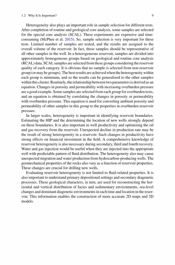
Although facies change is the main reason for heterogeneity in a carbonate reser-voir, its variations are routinely observed in meter to tens of meter scale. In contrast,diagenetic processes modify the rock properties at smaller scales. These processesstart just after deposition. Marine isopachous rim cements, micritization, dolomi-tization, anhydrite cementation, precipitation of calcite blocky cements, fracturing,chemical and mechanical compaction and dissolution are some important diage-netic processes in a carbonate reservoir. Diagenetic processes take place in marine,meteoric and burial realms with different effects on various parts of a facies. Whilearagonitic ooids are easily dissolved in meteoric diagenetic environment, interparti-cle low-magnesium calcite cements remain unaltered. Different mineralogy of var-ious shells also affects diagenetic processes and the heterogeneity of the reservoir(Fig. 1.4).
1.3 Sources of Heterogeneity 11
Fig. 1.4 Facies and diagenetic heterogeneity in a Permian–Triassic carbonate core from PersianGulf area. Alternation of grainstone (a, d, e, h, k, l) and mudstone (b, c, f, i, j) within 4 meters ofcores is observable. A packstone (g) is also present. Diagenetic changes are at microscopic scale.Different sizes of dolomite crystals in one thin section (a, b, c), different micritization processes onone sample (d) and different rates of dissolution on grains (k, l) are obvious. The scales of all thinsection images are the same as subfigure “a,” plane-polarized light
Jung and Aigner (2012) introduced six factors controlling carbonate geobodiesand so their reservoir quality. They include geological age (depo-time), type of car-bonate platform (depo-system), facies belts (depo-zone), 3D geometrical classifica-tion (depo-shape), building blocks of the depo-shape (depo-element) and carbonatelithofacies (depo-facies). Example of a depo-system is a carbonate ramp or rimmedshelf. Depo-zones are subenvironments such as intertidal or lagoon. Bars or moundsare examples of depo-shape, and their various subenvironments such as flank or crestare depo-elements. Finally, rock textures and allochems make the lithofacies. Dia-genetic processes must be included which have been ignored in this study. Theseprocesses usually follow the general trend of these factors, especially in the case ofearly diagenesis.
1.4 Materials
Which data sources are used for understanding various aspects of heterogeneityin a carbonate reservoir? Generally, two types of data are available from a reservoir
12 1 Reservoir Heterogeneity: An Introduction
including direct and indirect data. Direct data include information derived from coresand cuttings. Various data types such as geological (Tavakoli 2018), petrophysical(McPhee et al. 2015), geomechanical (Zoback 2007) and geochemical (Ramkumar2015) are derived from cores. Cores are the most reliable source of reservoir infor-mation. In addition, providing some types of data from other sources is not possible.Permeability and rock texture are some of these examples. Lithology, type and fre-quency of allochems, microscopic sedimentary features such as bioturbation, pres-ence of opaque minerals, laminations, mud cracks, brecciation and fenestral fabric ofthe samples, type and frequency of various pore types, fractures, cements and com-paction features are retrieved from thin section analysis. Macroscopic features suchas fractures, facies changes, large intraclasts, various types of surfaces, sedimentarystructures and large pores are recorded in macroscopic core description. Computedtomography scanning (CT scan) of the cores is used for identifying fractures andalso calculating some petrophysical properties. Various petrophysical properties arederived from cores in routine and special phases of a core analysis project. High-resolution sampling yields more information about the heterogeneity of the propertyof interest. Anyway, in a standard core analysis project, four samples are taken from1 m of core (Tavakoli 2018).
Cuttings are another source of direct information, but their application is limiteddue to the small sample sizes. Thin sections can be prepared from cuttings, but poretypes could not be distinguished. Running most of the routine tests is not possible oncuttings. During drilling, rocks continuously fall out and mix with the bottom holesamples.
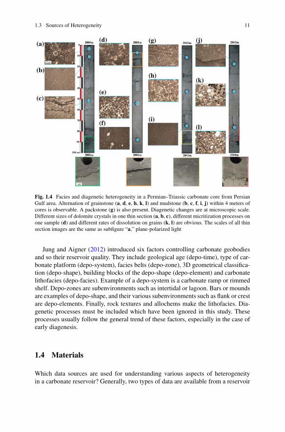
Wire-line logs and seismic data provide indirect measurements from rocks andfluids of the reservoir. Logs provide different types of information such as naturalgamma radiation, density, porosity, sonic velocity and electrical resistivity. Petro-physical analysis based on these data yields important information from the reservoir.The routine sampling interval is 0.1524m for these data. In contrast, seismic sectionsprovide information at larger scales. They are used for macroscopic to megascopicreservoir studies. Geometry of the reservoir, large structural features such as mainfaults, traps and contacts are some examples (Fig. 1.5).
1.5 Heterogeneity Scales
The heterogeneity concept is always accompanied by a specific scale. In fact, a sam-ple may be homogeneous at one scale and heterogeneous at another. A core plugmay be homogeneous with respect to its pore types, while the core itself is hetero-geneous. Heterogeneity hierarchies also depend on the property. While facies maybe homogeneous in 1 m of core, they vary considerably in well scale. Heterogeneityand homogeneity are end-members of a continuous spectrum. So, key units shouldbe defined to classify these hierarchies. Samples have different sizes, dependingon the objectives of the studies. The REV which was discussed in Sect. 1.1.1 is a
1.5 Heterogeneity Scales 13
Fig. 1.5 Various data types which are used for heterogeneity analysis of a carbonate reservoir. Theheterogeneity scale is also important, and so some of these classifications may change according tothe scale
mathematical representation of how the sample size plays an important role in itsheterogeneity.
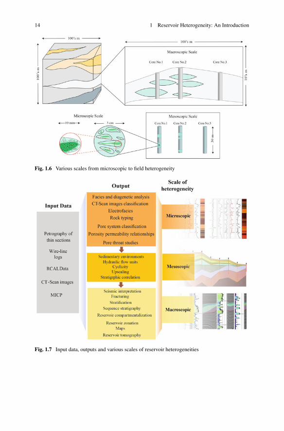
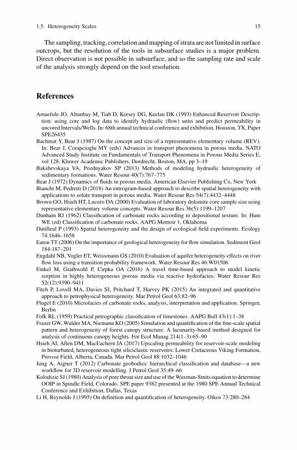
Heterogeneity exists at micro-, meso-, macro-, mega- and gigascales in a reser-voir. Microscopic heterogeneities include facies characteristics, diagenetic effects,pore types, pore throat sizes, grain shape, size and packing as well as mineralogyof the samples. These heterogeneities are measured using thin sections, scanningelectron microscope (SEM), mercury injection capillary pressure (MICP) tests, coreCT scanning and wire-line logs. Porosity–permeability relationships are presented,various classification schemes (such as pore typing) are applied to data, and electro-facies (EF) are defined fromwire-line logs to overcome the heterogeneity challengesat this scale. At mesoscopic scale, fine-scale data are integrated at well scale toconstruct traceable homogeneous units in the reservoir. Defining sedimentary envi-ronments and hydraulic flow units (HFUs), stratigraphic correlations and upscalingare some examples. Macroscopic heterogeneities include field-scale variables suchas stratification, compartmentalization, sequence stratigraphy, reservoir zonation andlateral property trends (Fig. 1.6). The megascopic scale of heterogeneity representsthe basin-scale parameters such as tectonic activities and the role of structural fea-tures as well as widespread depositional conditions. So, various data are combinedto understand the overall heterogeneity of a reservoir (Fig. 1.7).
14 1 Reservoir Heterogeneity: An Introduction
Fig. 1.6 Various scales from microscopic to field heterogeneity
Fig. 1.7 Input data, outputs and various scales of reservoir heterogeneities
1.5 Heterogeneity Scales 15
The sampling, tracking, correlation andmapping of strata are not limited in surfaceoutcrops, but the resolution of the tools in subsurface studies is a major problem.Direct observation is not possible in subsurface, and so the sampling rate and scaleof the analysis strongly depend on the tool resolution.
References
Amaefule JO, Altunbay M, Tiab D, Kersey DG, Keelan DK (1993) Enhanced Reservoir Descrip-tion: using core and log data to identify hydraulic (flow) units and predict permeability inuncored Intervals/Wells. In: 68th annual technical conference and exhibition. Houston, TX, PaperSPE26435
Bachmat Y, Bear J (1987) On the concept and size of a representative elementary volume (REV).In: Bear J, Corapcioglu MY (eds) Advances in transport phenomena in porous media. NATOAdvanced Study Institute on Fundamentals of Transport Phenomena in Porous Media Series E,vol 128. Kluwer Academic Publishers, Dordrecht, Boston, MA, pp 3–19
Bakshevskaya VA, Pozdnyakov SP (2013) Methods of modeling hydraulic heterogeneity ofsedimentary formations. Water Resour 40(7):767–775
Bear J (1972) Dynamics of fluids in porous media. American Elsevier Publishing Co, New YorkBianchi M, Pedretti D (2018) An entrogram-based approach to describe spatial heterogeneity withapplications to solute transport in porous media. Water Resour Res 54(7):4432–4448
Brown GO, Hsieh HT, Lucero DA (2000) Evaluation of laboratory dolomite core sample size usingrepresentative elementary volume concepts. Water Resour Res 36(5):1199–1207
Dunham RJ (1962) Classification of carbonate rocks according to depositional texture. In: HamWE (ed) Classification of carbonate rocks. AAPG Memoir 1, Oklahoma
Dutilleul P (1993) Spatial heterogeneity and the design of ecological field experiments. Ecology74:1646–1658
Eaton TT (2006) On the importance of geological heterogeneity for flow simulation. Sediment Geol184:187–201
Engdahl NB, Vogler ET, Weissmann GS (2010) Evaluation of aquifer heterogeneity effects on riverflow loss using a transition probability framework. Water Resour Res 46:W01506
Finkel M, Grathwohl P, Cirpka OA (2016) A travel time-based approach to model kineticsorption in highly heterogeneous porous media via reactive hydrofacies. Water Resour Res52(12):9390–9411
Fitch P, Lovell MA, Davies SJ, Pritchard T, Harvey PK (2015) An integrated and quantitativeapproach to petrophysical heterogeneity. Mar Petrol Geol 63:82–96
Flugel E (2010) Microfacies of carbonate rocks, analysis, interpretation and application. Springer,Berlin
Folk RL (1959) Practical petrographic classification of limestones. AAPG Bull 43(1):1–38Frazer GW,WulderMA, Niemann KO (2005) Simulation and quantification of the fine-scale spatialpattern and heterogeneity of forest canopy structure: A lacunarity-based method designed foranalysis of continuous canopy heights. For Ecol Manag 214(1–3):65–90
Hsieh AI, Allen DM, MacEachern JA (2017) Upscaling permeability for reservoir-scale modelingin bioturbated, heterogeneous tight siliciclastic reservoirs: Lower Cretaceous Viking Formation,Provost Field, Alberta, Canada. Mar Petrol Geol 88:1032–1046
Jung A, Aigner T (2012) Carbonate geobodies: hierarchical classification and database—a newworkflow for 3D reservoir modelling. J Petrol Geol 35:49–66
Kolodizie SJ (1980)Analysis of pore throat size and use of theWaxman-Smits equation to determineOOIP in Spindle Field, Colorado. SPE paper 9382 presented at the 1980 SPE Annual TechnicalConference and Exhibition, Dallas, Texas
Li H, Reynolds J (1995) On definition and quantification of heterogeneity. Oikos 73:280–284

16 1 Reservoir Heterogeneity: An Introduction
Lucia FJ (1995) Rock-fabric/petrophysical classification of carbonate pore space for reservoircharacterization. Am Assoc Petr Geol B 79(9):1275–1300
Lucia FJ, Conti RD (1987) Rock fabric, permeability, and log relationships in an upward-shoaling,vuggy carbonate sequence. Bureau of Econ Geol Geol Circular 87–5
McPhee C, Reed J, Zubizarreta I (2015) Core analysis: a best practice guide. Elsevier, UKNazemi M, Tavakoli V, Rahimpour-Bonab H, Hosseini M, Sharifi-Yazdi M (2018) The effect ofcarbonate reservoir heterogeneity on Archie’s exponents (a and m), an example fromKangan andDalan gas formations in the central Persian Gulf. J Nat Gas Sci Eng 59:297–308
Nordahl K, Ringrose PS (2008) Identifying the representative elementary volume for permeabilityin heterolithic deposits using numerical rock models. Math Geol 40(7):753–771
Poeter EP, Gaylord DR (1990) Influence of aquifer heterogeneity on contaminant transport at theHanford Site. Ground Water 28(6):900–909
Ramkumar Mu (ed) (2015) Chemostratigraphy: concepts, techniques and application. Elsevier,Amsterdam
Song X, Chen X, Ye M, Dai Z, Hammond G, Zachara JM (2019) Delineating facies spatial dis-tribution by integrating ensemble data assimilation and indicator geostatistics with level-settransformation. Water Resour Res 55:2652–2671
Tavakoli V (2018) Geological core analysis: application to reservoir characterization. Springer,Cham, Switzerland
Tiab D, Donaldson EC (2015) Petrophysics, theory and practice of measuring reservoir rock andfluid transport properties. Gulf Professional Publishing, Houston
Vik B, Bastesen E, Skauge A (2013) Evaluation of representative elementary volume for a vuggycarbonate rock—part: porosity, permeability, and dispersivity. J Petrol Sci Eng 112:36–47
Walker RG (1984) General introduction: facies, facies sequences and facies models. In: WalkerRG (ed) Facies models, 2nd edn. Geological Association of Canada, Geoscience Canada ReprintSeries 1
Weber KJ (1986) How heterogeneity affects oil recovery. In: Lake LW, Carroll HB (eds) Reservoircharacterization. Academic Press, New York, pp 487–544
Zhengquan W, Qingeheng W, Yandong Z (1997) Quantification of spatial heterogeneity in oldgrowth forests of Korean Pine. J For Res 8:65–69
Zoback MD (2007) Reservoir Geomechanics. University Press, Cambridge, England
Chapter 2Microscopic Heterogeneity
Abstract Heterogeneity is variation in space and time which strongly depends onthe scale of the study. This chapter focuses on microscale heterogeneities in a car-bonate reservoir. At first, available data and methods are discussed to understand themicroscopic heterogeneity in carbonates. Then, various methods are introduced toovercome this challenge.All reservoir properties depend on geological attributes, andso facies analysis and diagenetic impacts on the carbonate reservoirs are discussed.Facies grouping and diagenetic facies are introduced to classify different geologi-cal properties into similar categorizes. CT scan images are used for classifying thesamples. Intelligent systems are widely used for this purpose. Porosity–permeabilityrelationships are one of the most important criteria which are used for understandingthe homogeneity of a unit. This is different for limy and dolomitic reservoirs. Inter-particle, moldic and vuggy porosities with completely different petrophysical behav-iors are dominant in limy carbonate reservoirs. Intercrystalline porosities betweendolomite crystals generally increase the homogeneity of a sample, but the resultalso depends on the type and amount of dolomitization. In contrast to limy reser-voirs, dolostones have small but uniform pore throat size distribution. Pore systemclassifications, rock typing methods and electrofacies are used for managing the het-erogeneity in microscale. Pore types significantly control the petrophysical behaviorof the carbonate reservoirs. They have been divided into various groups from dif-ferent points of view. Rock typing procedure starts with the study of geologicalproperties and continues with the incorporation of the petrophysical characteristicsof the samples. Wire-line log data are grouped based on their similar readings andthen are correlated with the previously determined rock types. The final unit is usedfor predicting reservoir properties in 3D space between the wells.
2.1 Facies Analysis
Facies is a set of properties which characterize a sedimentary rock sample. Theterm introduced by Gressly (1838) for the first time and has been the subject ofconsiderable debate so far. Recently, the term microfacies was defined by Flugel(2010) as all characters of a carbonate sample from thin section properties to hand
© The Author(s), under exclusive license to Springer Nature Switzerland AG 2020V. Tavakoli, Carbonate Reservoir Heterogeneity,SpringerBriefs in Petroleum Geoscience & Engineering,https://doi.org/10.1007/978-3-030-34773-4_2
17
18 2 Microscopic Heterogeneity
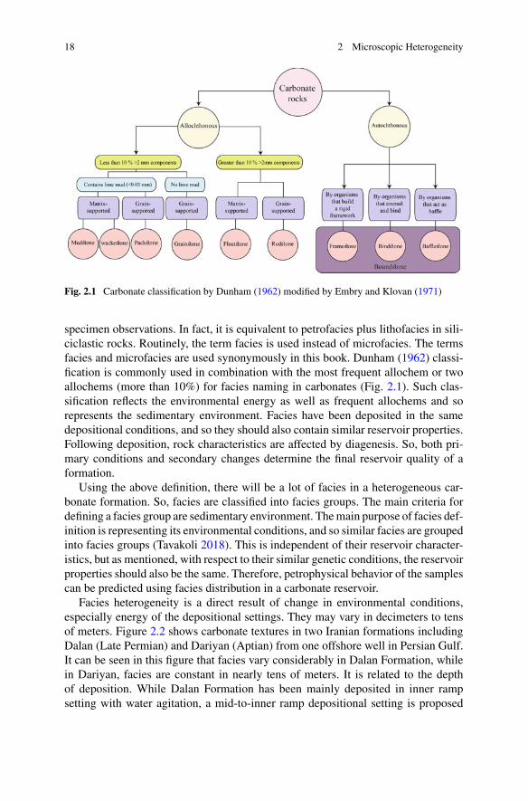
Fig. 2.1 Carbonate classification by Dunham (1962) modified by Embry and Klovan (1971)
specimen observations. In fact, it is equivalent to petrofacies plus lithofacies in sili-ciclastic rocks. Routinely, the term facies is used instead of microfacies. The termsfacies and microfacies are used synonymously in this book. Dunham (1962) classi-fication is commonly used in combination with the most frequent allochem or twoallochems (more than 10%) for facies naming in carbonates (Fig. 2.1). Such clas-sification reflects the environmental energy as well as frequent allochems and sorepresents the sedimentary environment. Facies have been deposited in the samedepositional conditions, and so they should also contain similar reservoir properties.Following deposition, rock characteristics are affected by diagenesis. So, both pri-mary conditions and secondary changes determine the final reservoir quality of aformation.
Using the above definition, there will be a lot of facies in a heterogeneous car-bonate formation. So, facies are classified into facies groups. The main criteria fordefining a facies group are sedimentary environment. Themain purpose of facies def-inition is representing its environmental conditions, and so similar facies are groupedinto facies groups (Tavakoli 2018). This is independent of their reservoir character-istics, but as mentioned, with respect to their similar genetic conditions, the reservoirproperties should also be the same. Therefore, petrophysical behavior of the samplescan be predicted using facies distribution in a carbonate reservoir.
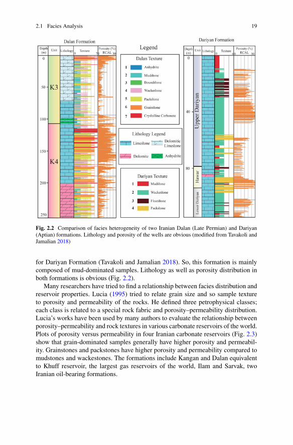
Facies heterogeneity is a direct result of change in environmental conditions,especially energy of the depositional settings. They may vary in decimeters to tensof meters. Figure 2.2 shows carbonate textures in two Iranian formations includingDalan (Late Permian) and Dariyan (Aptian) from one offshore well in Persian Gulf.It can be seen in this figure that facies vary considerably in Dalan Formation, whilein Dariyan, facies are constant in nearly tens of meters. It is related to the depthof deposition. While Dalan Formation has been mainly deposited in inner rampsetting with water agitation, a mid-to-inner ramp depositional setting is proposed
2.1 Facies Analysis 19
Fig. 2.2 Comparison of facies heterogeneity of two Iranian Dalan (Late Permian) and Dariyan(Aptian) formations. Lithology and porosity of the wells are obvious (modified from Tavakoli andJamalian 2018)
for Dariyan Formation (Tavakoli and Jamalian 2018). So, this formation is mainlycomposed of mud-dominated samples. Lithology as well as porosity distribution inboth formations is obvious (Fig. 2.2).
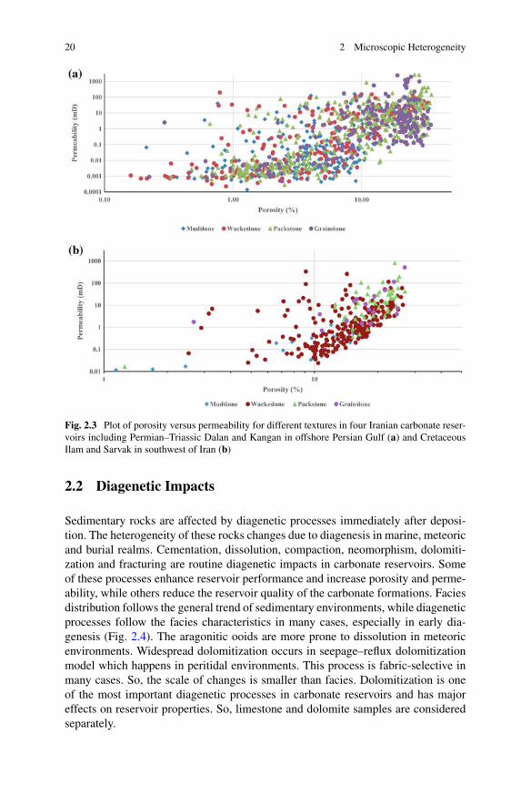
Many researchers have tried to find a relationship between facies distribution andreservoir properties. Lucia (1995) tried to relate grain size and so sample textureto porosity and permeability of the rocks. He defined three petrophysical classes;each class is related to a special rock fabric and porosity–permeability distribution.Lucia’s works have been used by many authors to evaluate the relationship betweenporosity–permeability and rock textures in various carbonate reservoirs of the world.Plots of porosity versus permeability in four Iranian carbonate reservoirs (Fig. 2.3)show that grain-dominated samples generally have higher porosity and permeabil-ity. Grainstones and packstones have higher porosity and permeability compared tomudstones and wackestones. The formations include Kangan and Dalan equivalentto Khuff reservoir, the largest gas reservoirs of the world, Ilam and Sarvak, twoIranian oil-bearing formations.
20 2 Microscopic Heterogeneity
Fig. 2.3 Plot of porosity versus permeability for different textures in four Iranian carbonate reser-voirs including Permian–Triassic Dalan and Kangan in offshore Persian Gulf (a) and CretaceousIlam and Sarvak in southwest of Iran (b)
2.2 Diagenetic Impacts
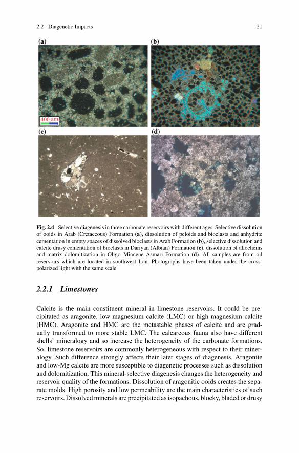
Sedimentary rocks are affected by diagenetic processes immediately after deposi-tion. The heterogeneity of these rocks changes due to diagenesis in marine, meteoricand burial realms. Cementation, dissolution, compaction, neomorphism, dolomiti-zation and fracturing are routine diagenetic impacts in carbonate reservoirs. Someof these processes enhance reservoir performance and increase porosity and perme-ability, while others reduce the reservoir quality of the carbonate formations. Faciesdistribution follows the general trend of sedimentary environments, while diageneticprocesses follow the facies characteristics in many cases, especially in early dia-genesis (Fig. 2.4). The aragonitic ooids are more prone to dissolution in meteoricenvironments. Widespread dolomitization occurs in seepage–reflux dolomitizationmodel which happens in peritidal environments. This process is fabric-selective inmany cases. So, the scale of changes is smaller than facies. Dolomitization is oneof the most important diagenetic processes in carbonate reservoirs and has majoreffects on reservoir properties. So, limestone and dolomite samples are consideredseparately.
2.2 Diagenetic Impacts 21
Fig. 2.4 Selective diagenesis in three carbonate reservoirs with different ages. Selective dissolutionof ooids in Arab (Cretaceous) Formation (a), dissolution of peloids and bioclasts and anhydritecementation in empty spaces of dissolved bioclasts in Arab Formation (b), selective dissolution andcalcite drusy cementation of bioclasts in Dariyan (Albian) Formation (c), dissolution of allochemsand matrix dolomitization in Oligo–Miocene Asmari Formation (d). All samples are from oilreservoirs which are located in southwest Iran. Photographs have been taken under the cross-polarized light with the same scale
2.2.1 Limestones
Calcite is the main constituent mineral in limestone reservoirs. It could be pre-cipitated as aragonite, low-magnesium calcite (LMC) or high-magnesium calcite(HMC). Aragonite and HMC are the metastable phases of calcite and are grad-ually transformed to more stable LMC. The calcareous fauna also have differentshells’ mineralogy and so increase the heterogeneity of the carbonate formations.So, limestone reservoirs are commonly heterogeneous with respect to their miner-alogy. Such difference strongly affects their later stages of diagenesis. Aragoniteand low-Mg calcite are more susceptible to diagenetic processes such as dissolutionand dolomitization. This mineral-selective diagenesis changes the heterogeneity andreservoir quality of the formations. Dissolution of aragonitic ooids creates the sepa-rate molds. High porosity and low permeability are the main characteristics of suchreservoirs. Dissolvedminerals are precipitated as isopachous, blocky, bladed or drusy
22 2 Microscopic Heterogeneity
cements. Calcite cementation also changes the heterogeneity of the carbonate sam-ples at microscopic scales. Isopachous cements retain the original framework of thesamples. They build a solid structure by binding the allochems in grain-dominatedsamples. Such cementation prevents later compaction and so maintains the facieshomogeneity of the samples. In contrast, blocky cements are precipitated in largerpores (Ehrenberg andWalderhaug2015), and so this typeof cementation increases theheterogeneity of the carbonate formations. Micrite particles are subjected to aggrad-ing neomorphism. Original fabrics of carbonate allochems are altered to micrite inmarine environments. It may affect the whole allochem or just its crust and makemicrite envelope around the grains. This envelope prevents more diagenetic impacts(such as compaction) on allochems. Lamination is not a routine structure in carbonaterocks, but it is present in some cases. For example, stromatolites have original lami-nated structures. They generally live in peritidal environments but can also developto lower intertidal or even other shallow environments (Tavakoli et al. 2018). Deposi-tion of micrite particles in calm lagoonal conditions also creates fine laminae in thesedeposits. In such laminations, geological and petrophysical properties are nearly thesame in horizontal direction but they are strongly different in vertical column.
Bioturbations also increase heterogeneity in carbonate strata. This process can alsochange the reservoir properties. Fenestral fabrics are mainly arranged concordant tostratification and increase the porosity of the samples if they are not filled withcements. This type of porosity has no strong effect on reservoir development. Theeffects of some other factors such as mud cracks, opaque minerals and brecciationare also negligible.
Routinely, there are various pore types in a carbonates formation. The primaryinterparticle porosities are uniformly distributed in the rocks. They are formed pri-marily in high-energy depositional settings and are seen in grain-dominated textures.In contrast, distribution of secondary porosities such as moldic and vuggy is not uni-form. They generally affect the rocks according to their original mineralogy whichis different for various allochems. Fractures crosscut the cements, matrix and alsoallochems. They increase heterogeneity of the formations especially at the time ofproduction. The fracturing process and its effect on carbonate reservoir heterogeneityare discussed in Sect. 4.2.
Physical compaction affects the rocks in greater depths of burial. The result ofsuch compaction is porosity reduction, broken grains, concave–convex contacts andbending of ductile grains. Chemical compaction-related structures have strong effectson reservoir properties (e.g., Bruna et al. 2019). Their formation, frequency andorientation strongly depend on principal stress direction of the area. This is lithostaticpressure in many cases, and so they are parallel to lamination. Generally, stylolitesand solution seams are flow barriers and so reduce permeability (e.g., Mehrabi et al.2016). Stylolites also may leak depending on collecting material and the size ofspikes (Koehn et al. 2016). So, they change the heterogeneity of the reservoir rocks.The important point is that their past and present-day impacts on reservoir quality ofthe carbonate formations are different (Bruna et al. 2019).
2.2 Diagenetic Impacts 23
2.2.2 Dolomitic Reservoirs
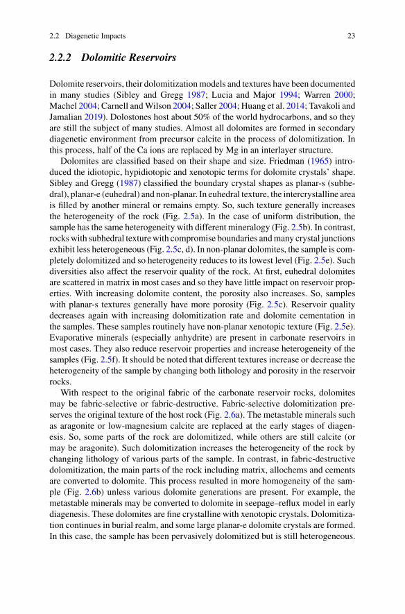
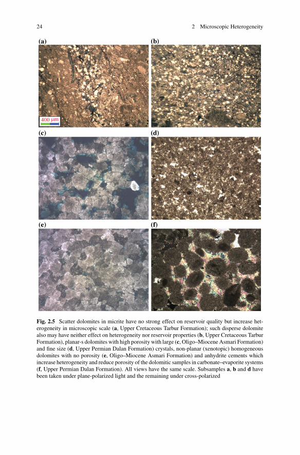
Dolomite reservoirs, their dolomitizationmodels and textures have been documentedin many studies (Sibley and Gregg 1987; Lucia and Major 1994; Warren 2000;Machel 2004; Carnell andWilson 2004; Saller 2004; Huang et al. 2014; Tavakoli andJamalian 2019). Dolostones host about 50% of the world hydrocarbons, and so theyare still the subject of many studies. Almost all dolomites are formed in secondarydiagenetic environment from precursor calcite in the process of dolomitization. Inthis process, half of the Ca ions are replaced by Mg in an interlayer structure.
Dolomites are classified based on their shape and size. Friedman (1965) intro-duced the idiotopic, hypidiotopic and xenotopic terms for dolomite crystals’ shape.Sibley and Gregg (1987) classified the boundary crystal shapes as planar-s (subhe-dral), planar-e (euhedral) and non-planar. In euhedral texture, the intercrystalline areais filled by another mineral or remains empty. So, such texture generally increasesthe heterogeneity of the rock (Fig. 2.5a). In the case of uniform distribution, thesample has the same heterogeneity with different mineralogy (Fig. 2.5b). In contrast,rockswith subhedral texturewith compromise boundaries andmany crystal junctionsexhibit less heterogeneous (Fig. 2.5c, d). In non-planar dolomites, the sample is com-pletely dolomitized and so heterogeneity reduces to its lowest level (Fig. 2.5e). Suchdiversities also affect the reservoir quality of the rock. At first, euhedral dolomitesare scattered in matrix in most cases and so they have little impact on reservoir prop-erties. With increasing dolomite content, the porosity also increases. So, sampleswith planar-s textures generally have more porosity (Fig. 2.5c). Reservoir qualitydecreases again with increasing dolomitization rate and dolomite cementation inthe samples. These samples routinely have non-planar xenotopic texture (Fig. 2.5e).Evaporative minerals (especially anhydrite) are present in carbonate reservoirs inmost cases. They also reduce reservoir properties and increase heterogeneity of thesamples (Fig. 2.5f). It should be noted that different textures increase or decrease theheterogeneity of the sample by changing both lithology and porosity in the reservoirrocks.
With respect to the original fabric of the carbonate reservoir rocks, dolomitesmay be fabric-selective or fabric-destructive. Fabric-selective dolomitization pre-serves the original texture of the host rock (Fig. 2.6a). The metastable minerals suchas aragonite or low-magnesium calcite are replaced at the early stages of diagen-esis. So, some parts of the rock are dolomitized, while others are still calcite (ormay be aragonite). Such dolomitization increases the heterogeneity of the rock bychanging lithology of various parts of the sample. In contrast, in fabric-destructivedolomitization, the main parts of the rock including matrix, allochems and cementsare converted to dolomite. This process resulted in more homogeneity of the sam-ple (Fig. 2.6b) unless various dolomite generations are present. For example, themetastable minerals may be converted to dolomite in seepage–reflux model in earlydiagenesis. These dolomites are fine crystalline with xenotopic crystals. Dolomitiza-tion continues in burial realm, and some large planar-e dolomite crystals are formed.In this case, the sample has been pervasively dolomitized but is still heterogeneous.
24 2 Microscopic Heterogeneity
Fig. 2.5 Scatter dolomites in micrite have no strong effect on reservoir quality but increase het-erogeneity in microscopic scale (a, Upper Cretaceous Tarbur Formation); such disperse dolomitealso may have neither effect on heterogeneity nor reservoir properties (b, Upper Cretaceous TarburFormation), planar-s dolomites with high porosity with large (c, Oligo–Miocene Asmari Formation)and fine size (d, Upper Permian Dalan Formation) crystals, non-planar (xenotopic) homogeneousdolomites with no porosity (e, Oligo–Miocene Asmari Formation) and anhydrite cements whichincrease heterogeneity and reduce porosity of the dolomitic samples in carbonate–evaporite systems(f, Upper Permian Dalan Formation). All views have the same scale. Subsamples a, b and d havebeen taken under plane-polarized light and the remaining under cross-polarized

2.2 Diagenetic Impacts 25
Fig. 2.6 Fabric-selective dolomitization in Early Triassic Kangan Formation (a, plane-polarized),fabric-destructive dolomitization in Oligo–Miocene Asmari Formation (b, cross-polarized). Ghostof a bioclast is still visible after pervasive dolomitization (arrow). Two views have the same scale
The origin of porosity in dolomitic reservoirs is still controversial. It may berelated to dolomitization process or inherited from the precursor limestones (Purseret al. 1994). Inmole-for-mole dolomitization up to 13%porosity is generated (TuckerandWright 1990;Machel 2004). Some researchers (e.g., Saller and Henderson 1998,2001) believe that in the volume-for-volume replacement, porosity can be constantor even decreases. Combining previous studies, it can be concluded that the porosityof the precursor limestones increases during dolomitization process (Tavakoli andJamalian 2019). So, some part of the porosity is inherited from primary depositionalfabric, while another part is developed during dolomitization. Dolomitization createsintercrystalline porosity or enhances the primary interparticle porosities (Tucker andWright 1990;Machel 2004; Tavakoli and Jamalian 2019). Both of these pore types areconnected, and so permeability also increases during this process. This leads to lessheterogeneity in carbonate reservoirs because it improves the porosity–permeabilityrelationships. Both early and late dolomites have the same effect from this point ofview. It is obvious that the dolomite fabric is also important in each case.
2.2.3 Diagenetic Facies
Diagenesis has a strong effect on reservoir properties and can decrease or increasethe porosity and permeability of the carbonates. So, defining a unit with similardiagenetic characteristics is useful in considering reservoir heterogeneity. From thedefinition of the term “facies” (Gressly 1838), it can be concluded that diageneticfacies refers to the rocks with the same diagenetic impacts. In fact, such as faciesitself, the diagenetic facies is also defined to classify the reservoir rocks based ontheir diagenetic properties. Zou and his co-workers (2008) believed that with respectto the effect on reservoir properties, there are two types of diagenetic facies includ-ing constructive and destructive. These are the result of combined effect of structure,
26 2 Microscopic Heterogeneity
fluids, temperature and pressure on precursor sediments. The rock properties of thesamples within these groups routinely have the same depositional characteristics, andso the groups can be used for determining spatial distribution of reservoir parame-ters. The main data source for classifying diagenetic facies is core and equivalentoutcrop sections. Efforts have been made to relate diagenetic processes and impactsto wire-line logs (such as Cui et al. 2017; Lai et al. 2019). The samples can be classi-fied based on diagenetic minerals, processes and environments. The main diageneticmineral in carbonates is dolomite which has been discussed in Sect. 2.2.2. The maindiagenetic processes are micritization, recrystallization, marine cementation, disso-lution, dolomitization, compaction (physical and chemical), burial cementation andfracturing. Three diagenetic environments in carbonates include marine, meteoricand burial. Diagenetic processes are discussed within the framework of their envi-ronments. In many cases, meteoric and shallow burial diagenesis enhances reservoirproperties, while burial processes decrease both porosity and permeability of thesamples. Fracturing in late diagenetic environment increases the permeability ofthe rocks. Burial dissolution is exceptionally effective in porosity and permeabilityenhancement in carbonate reservoirs.
Reservoir quality is themost important criteria for classifying the samples in a car-bonate reservoir. So, a diagenetic facies is routinely defined based on its constructiveor destructive effects on reservoir properties. Themain constructive processes includedissolution and dolomitization which create moldic and intercrystalline porosity,respectively. Destructive processes are compaction and cementation. The final reser-voir quality is the result of both primary facies characteristics as well as secondarydiagenetic changes, and so both of them should be considered to define a repre-sentative unit. Wang and his co-workers (2017) based on their work in a sandstonereservoir defined the sedimentary–diagenetic facies as a combination of litho- anddiagenetic facies. In carbonate reservoirs, a sedimentary–diagenetic facies is definedas a combination of micro- and diagenetic facies. It is more useful in understandingthe heterogeneity of a reservoir, as it integrates the effects of both variables. Var-ious primary characteristics as well as diagenetic processes influence a carbonatereservoir. Accordingly, definition of such facies is complicated (Fig. 2.7). In fact,this definition is very close to the concept of geological rock type (GRT) (Tavakoli2018).
Such as any other homogeneous unit, the diagenetic facies should be investigatedat microscale and then expand to meso- and macroscale through macroscopic coreanalysis, comparison with wire-line log data, upscaling, stratigraphic correlation,mapping and statistical modeling (Fig. 2.8). They also can be used for more accurateprediction of reservoir properties, such as permeability. Each diagenetic facies canhave its specific formula with particular coefficients for such predictions.
2.2.4 Quantitative Diagenesis
Quantitative data are required to define a representative unit for understandingreservoir heterogeneity and prediction of reservoir properties in a 3D space. Many
2.2 Diagenetic Impacts 27
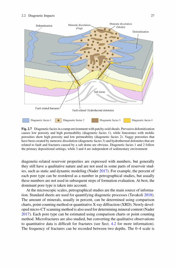
Fig. 2.7 Diagenetic facies in a ramp environment with patchy ooid shoals. Pervasive dolomitizationcauses low porosity and high permeability (diagenetic facies 1), while limestones with moldicporosities show high porosity and low permeability (diagenetic facies 2). Vuggy porosities thathave been created by meteoric dissolution (diagenetic facies 3) and hydrothermal dolomites that arerelated to fault and fractures caused by a salt dome are obvious. Diagenetic facies 1 and 2 followthe primary depositional settings, while 3 and 4 are independent of sedimentary environment
diagenetic-related reservoir properties are expressed with numbers, but generallythey still have a qualitative nature and are not used in some parts of reservoir stud-ies, such as static and dynamic modeling (Nader 2017). For example, the percent ofeach pore type can be reordered as a number in petrographical studies, but usuallythese numbers are not used in subsequent steps of formation evaluation. At best, thedominant pore type is taken into account.
At the microscopic scales, petrographical studies are the main source of informa-tion. Standard sheets are used for quantifying diagenetic processes (Tavakoli 2018).The amount of minerals, usually in percent, can be determined using comparisoncharts, point counting method or quantitative X-ray diffraction (XRD). Newly devel-opedmicro-CT scanningmethod is also used for determiningmineral content (Nader2017). Each pore type can be estimated using comparison charts or point countingmethod. Microfractures are also studied, but converting the qualitative observationsto quantitative data is difficult for fractures (see Sect. 4.2 for more information).The frequency of fractures can be recorded between two depths. The 0–4 scale is
28 2 Microscopic Heterogeneity
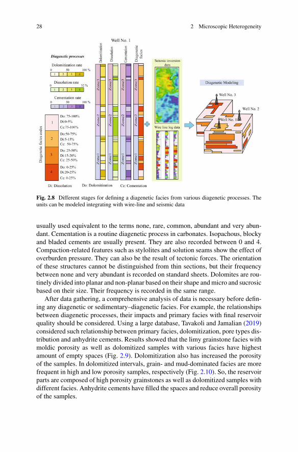
Fig. 2.8 Different stages for defining a diagenetic facies from various diagenetic processes. Theunits can be modeled integrating with wire-line and seismic data
usually used equivalent to the terms none, rare, common, abundant and very abun-dant. Cementation is a routine diagenetic process in carbonates. Isopachous, blockyand bladed cements are usually present. They are also recorded between 0 and 4.Compaction-related features such as stylolites and solution seams show the effect ofoverburden pressure. They can also be the result of tectonic forces. The orientationof these structures cannot be distinguished from thin sections, but their frequencybetween none and very abundant is recorded on standard sheets. Dolomites are rou-tinely divided into planar and non-planar based on their shape andmicro and sucrosicbased on their size. Their frequency is recorded in the same range.
After data gathering, a comprehensive analysis of data is necessary before defin-ing any diagenetic or sedimentary–diagenetic facies. For example, the relationshipsbetween diagenetic processes, their impacts and primary facies with final reservoirquality should be considered. Using a large database, Tavakoli and Jamalian (2019)considered such relationship between primary facies, dolomitization, pore types dis-tribution and anhydrite cements. Results showed that the limy grainstone facies withmoldic porosity as well as dolomitized samples with various facies have highestamount of empty spaces (Fig. 2.9). Dolomitization also has increased the porosityof the samples. In dolomitized intervals, grain- and mud-dominated facies are morefrequent in high and low porosity samples, respectively (Fig. 2.10). So, the reservoirparts are composed of high porosity grainstones as well as dolomitized samples withdifferent facies. Anhydrite cements have filled the spaces and reduce overall porosityof the samples.
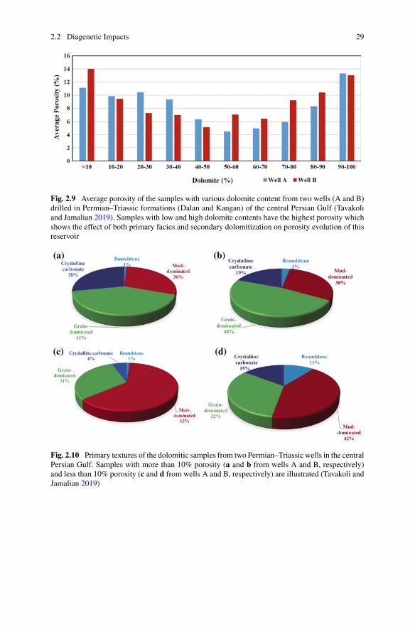
2.2 Diagenetic Impacts 29
Fig. 2.9 Average porosity of the samples with various dolomite content from two wells (A and B)drilled in Permian–Triassic formations (Dalan and Kangan) of the central Persian Gulf (Tavakoliand Jamalian 2019). Samples with low and high dolomite contents have the highest porosity whichshows the effect of both primary facies and secondary dolomitization on porosity evolution of thisreservoir
Fig. 2.10 Primary textures of the dolomitic samples from two Permian–Triassic wells in the centralPersian Gulf. Samples with more than 10% porosity (a and b from wells A and B, respectively)and less than 10% porosity (c and d from wells A and B, respectively) are illustrated (Tavakoli andJamalian 2019)
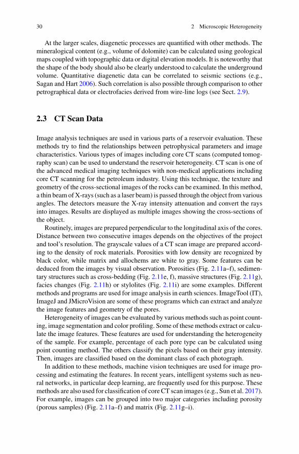
30 2 Microscopic Heterogeneity
At the larger scales, diagenetic processes are quantified with other methods. Themineralogical content (e.g., volume of dolomite) can be calculated using geologicalmaps coupled with topographic data or digital elevation models. It is noteworthy thatthe shape of the body should also be clearly understood to calculate the undergroundvolume. Quantitative diagenetic data can be correlated to seismic sections (e.g.,Sagan and Hart 2006). Such correlation is also possible through comparison to otherpetrographical data or electrofacies derived from wire-line logs (see Sect. 2.9).
2.3 CT Scan Data
Image analysis techniques are used in various parts of a reservoir evaluation. Thesemethods try to find the relationships between petrophysical parameters and imagecharacteristics. Various types of images including core CT scans (computed tomog-raphy scan) can be used to understand the reservoir heterogeneity. CT scan is one ofthe advanced medical imaging techniques with non-medical applications includingcore CT scanning for the petroleum industry. Using this technique, the texture andgeometry of the cross-sectional images of the rocks can be examined. In this method,a thin beam ofX-rays (such as a laser beam) is passed through the object from variousangles. The detectors measure the X-ray intensity attenuation and convert the raysinto images. Results are displayed as multiple images showing the cross-sections ofthe object.
Routinely, images are prepared perpendicular to the longitudinal axis of the cores.Distance between two consecutive images depends on the objectives of the projectand tool’s resolution. The grayscale values of a CT scan image are prepared accord-ing to the density of rock materials. Porosities with low density are recognized byblack color, while matrix and allochems are white to gray. Some features can bededuced from the images by visual observation. Porosities (Fig. 2.11a–f), sedimen-tary structures such as cross-bedding (Fig. 2.11e, f), massive structures (Fig. 2.11g),facies changes (Fig. 2.11h) or stylolites (Fig. 2.11i) are some examples. Differentmethods and programs are used for image analysis in earth sciences. ImageTool (IT),ImageJ and JMicroVision are some of these programs which can extract and analyzethe image features and geometry of the pores.
Heterogeneity of images can be evaluated by variousmethods such as point count-ing, image segmentation and color profiling. Some of these methods extract or calcu-late the image features. These features are used for understanding the heterogeneityof the sample. For example, percentage of each pore type can be calculated usingpoint counting method. The others classify the pixels based on their gray intensity.Then, images are classified based on the dominant class of each photograph.
In addition to these methods, machine vision techniques are used for image pro-cessing and estimating the features. In recent years, intelligent systems such as neu-ral networks, in particular deep learning, are frequently used for this purpose. Thesemethods are also used for classification of core CT scan images (e.g., Sun et al. 2017).For example, images can be grouped into two major categories including porosity(porous samples) (Fig. 2.11a–f) and matrix (Fig. 2.11g–i).
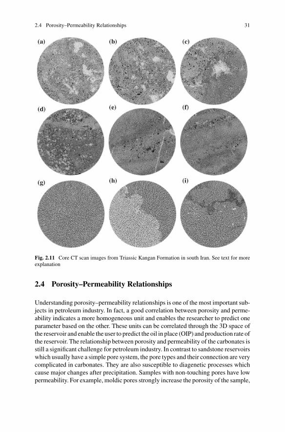
2.4 Porosity–Permeability Relationships 31
Fig. 2.11 Core CT scan images from Triassic Kangan Formation in south Iran. See text for moreexplanation
2.4 Porosity–Permeability Relationships
Understanding porosity–permeability relationships is one of the most important sub-jects in petroleum industry. In fact, a good correlation between porosity and perme-ability indicates a more homogeneous unit and enables the researcher to predict oneparameter based on the other. These units can be correlated through the 3D space ofthe reservoir and enable the user to predict the oil in place (OIP) and production rate ofthe reservoir. The relationship between porosity and permeability of the carbonates isstill a significant challenge for petroleum industry. In contrast to sandstone reservoirswhich usually have a simple pore system, the pore types and their connection are verycomplicated in carbonates. They are also susceptible to diagenetic processes whichcause major changes after precipitation. Samples with non-touching pores have lowpermeability. For example, moldic pores strongly increase the porosity of the sample,
32 2 Microscopic Heterogeneity
while it has no strong effect on permeability. Conversely, both porosity and perme-ability increase through dolomitization process, but its effect on permeability is moresignificant. Many researchers tried to introduce a pore system classification based onsuch relationships (e.g., Lucia 1995). From this point of view, porosities are classifiedinto connected and disconnected. Interparticle and intercrystalline pores are the mostfrequent connected pores, while moldic and vuggy are dominant disconnected poretypes in carbonates. Non-effective pores can be connected by some later diageneticprocesses such as dolomitization or fracturing.
The degree of correlation between porosity and permeability is always a usefulcriterion in recognizing the degree of homogeneity in a rock type. High coefficient ofdetermination (R2) value shows a good correlation and so effectiveness of the usedmethod and its ability to differentiate the samples based on the same reservoir prop-erties. There is no known equation to relate porosity and permeability in carbonatesystems, but efforts have been made to construct such relationship (e.g., Ehrenbergand Nadeau 2005). So, the R2 value of such relationship can be calculated based onany equation. The higher value indicates the more appropriate equation.
2.4.1 Limestones
The porosity–permeability relationships in limestones depend on many parameters.The original facies and fabric as well as diagenetic processes are responsible for thegoodness of fit between porosity and permeability. Originally, the grainstone facieshave higher porosity and permeability because of their interparticle pore spaces.This pore system is also homogeneous. In fact, the interparticle porosity betweenallochems is very similar to sandstone pore systems.After deposition, they are subjectto marine diagenesis. Isopachous rim cements build a rigid framework. They bindthe allochems to each other. These cements are just around the grains and so theyhave no strong effect on porosity or permeability of the samples. Micritization isa routine process in calm environments such as lagoon depositional setting. In thisprocess, the microspar and sparite are converted to micrite by bacterial activities.Micritization increases the amount ofmicrite and so themicroporosity of the samples.These samples have high porosity and low permeability. The Albian–Aptian DariyanFormation (equivalent to Shuaiba Formation in Arabian territories) in the PersianGulf area is a good example. The samples of this formation contain no visible porosityin petrographic studies (Naderi-Khujin et al. 2016), but wire-line log data and coreanalysis indicate the average of 15% porosity in the samples. The micropores havebeen developed inmeteoric diagenesis through partial dissolution of micrite particles(Tavakoli and Jamalian 2018). As microporosity is dominant pore system, a goodcorrelation can be seen between the porosity and permeability of the samples whichincreases the homogeneity of the rocks. Mud-dominated samples (mudstone andwackestone) have lower primary porosity and permeability. The micrite particles fillthe empty spaces. These samples can have high amounts of microporosity, which

2.4 Porosity–Permeability Relationships 33
discussed previously. Recently, a review of the genesis and distribution of limestonemicroporosity has been presented by Hashim and Kaczmarek (2019).
After marine diagenesis, samples are usually affected by meteoric waters. Thesewaters dissolve the unstable allochems such as aragonitic ooids and have a majorimpact on porosity development. Such diagenesis creates isolated molds which arenot connected to each other. So, porosity increases considerably while permeabil-ity is almost constant. There is no correlation between porosity and permeability ofthe samples. If moldic porosities are unique pore system in the sample, this pro-cess has negligible effect on reservoir heterogeneity in microscale. A combination ofvarious pore types causes different types of heterogeneity and also porosity–perme-ability relationships. Interparticle, intercrystalline or fracture porosities connect themoldic pores and so increase permeability alongwith porosity of the carbonate rocks.These pore types increase the geological heterogeneity of the samples and cause bet-ter porosity–permeability correlation of the samples. In contrast, separate molds orvugs may be accompanied by other disconnected pores such as micropores. Porositysignificantly increases in these cases, but permeability is nearly constant. Cemen-tations may occlude some of the larger pores and decrease the heterogeneity of thesamples. This appears to have happened in Dariyan and Shuaiba formations. Largemoldic pores have been developed by dissolution in early diagenetic phase. Micritesalso affected by meteoric waters, and both porosity and heterogeneity increased sig-nificantly. Large pores filled with calcite cements in late diagenesis, but microporesremained empty (Ehrenberg andWalderhaug 2015). This process not only decreasedthe amount of pore spaces but also the heterogeneity of the formation. The high R2
value between porosity and permeability in this formation clearly demonstrates thishomogeneity.
From the above discussion, it can be concluded that the poro–perm relationships incarbonates are affected by many parameters in various ways and so their correlationis not generally good. There is no known relationship between these two param-eters in carbonate reservoirs, as mentioned before. Figure 2.12 illustrates porosi-ty–permeability data from limestone samples (more than 90% lime) from 5 Iranianreservoirs includingDalan (Late Permian),Kangan (Early–Middle Triassic), Dariyan(Albian–Aptian), Sarvak (Albian–Turonian) and Ilam (Santonian–Campanian). Thebest correlation can be seen inDariyan Formationwith dominant microporosity. Ilamand Sarvak formations contain microporosity, interparticle and moldic pores. Kan-gan and Dalan formations have the weakest correlation. Various pore types includingmicroporosity, moldic, inter- and interaparticle, fenestral and intercrystalline poreshave been identified in these formations (Abdolmaleki et al. 2016).
2.4.2 Dolomites
Dolomites and dolomitization process have different effects on porosity–permeabil-ity relationships and reservoir heterogeneity. Many of these aspects discussed pre-viously (Sect. 2.2.2). Many researchers believe that dolomitization increases both
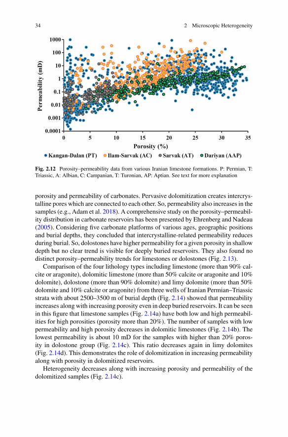
34 2 Microscopic Heterogeneity
Fig. 2.12 Porosity–permeability data from various Iranian limestone formations. P: Permian, T:Triassic, A: Albian, C: Campanian, T: Turonian, AP: Aptian. See text for more explanation
porosity and permeability of carbonates. Pervasive dolomitization creates intercrys-talline pores which are connected to each other. So, permeability also increases in thesamples (e.g., Adam et al. 2018). A comprehensive study on the porosity–permeabil-ity distribution in carbonate reservoirs has been presented by Ehrenberg and Nadeau(2005). Considering five carbonate platforms of various ages, geographic positionsand burial depths, they concluded that intercrystalline-related permeability reducesduring burial. So, dolostones have higher permeability for a given porosity in shallowdepth but no clear trend is visible for deeply buried reservoirs. They also found nodistinct porosity–permeability trends for limestones or dolostones (Fig. 2.13).
Comparison of the four lithology types including limestone (more than 90% cal-cite or aragonite), dolomitic limestone (more than 50% calcite or aragonite and 10%dolomite), dolostone (more than 90% dolomite) and limy dolomite (more than 50%dolomite and 10% calcite or aragonite) from three wells of Iranian Permian–Triassicstrata with about 2500–3500 m of burial depth (Fig. 2.14) showed that permeabilityincreases alongwith increasing porosity even in deep buried reservoirs. It can be seenin this figure that limestone samples (Fig. 2.14a) have both low and high permeabil-ities for high porosities (porosity more than 20%). The number of samples with lowpermeability and high porosity decreases in dolomitic limestones (Fig. 2.14b). Thelowest permeability is about 10 mD for the samples with higher than 20% poros-ity in dolostone group (Fig. 2.14c). This ratio decreases again in limy dolomites(Fig. 2.14d). This demonstrates the role of dolomitization in increasing permeabilityalong with porosity in dolomitized reservoirs.
Heterogeneity decreases along with increasing porosity and permeability of thedolomitized samples (Fig. 2.14c).
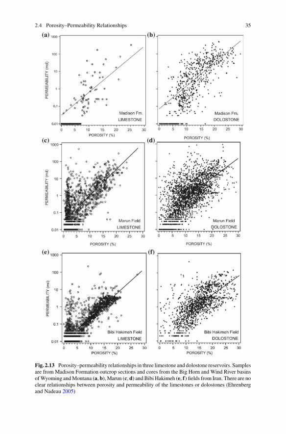
2.4 Porosity–Permeability Relationships 35
Fig. 2.13 Porosity–permeability relationships in three limestone and dolostone reservoirs. Samplesare from Madison Formation outcrop sections and cores from the Big Horn and Wind River basinsofWyoming andMontana (a, b), Marun (c, d) and Bibi Hakimeh (e, f) fields from Iran. There are noclear relationships between porosity and permeability of the limestones or dolostones (Ehrenbergand Nadeau 2005)
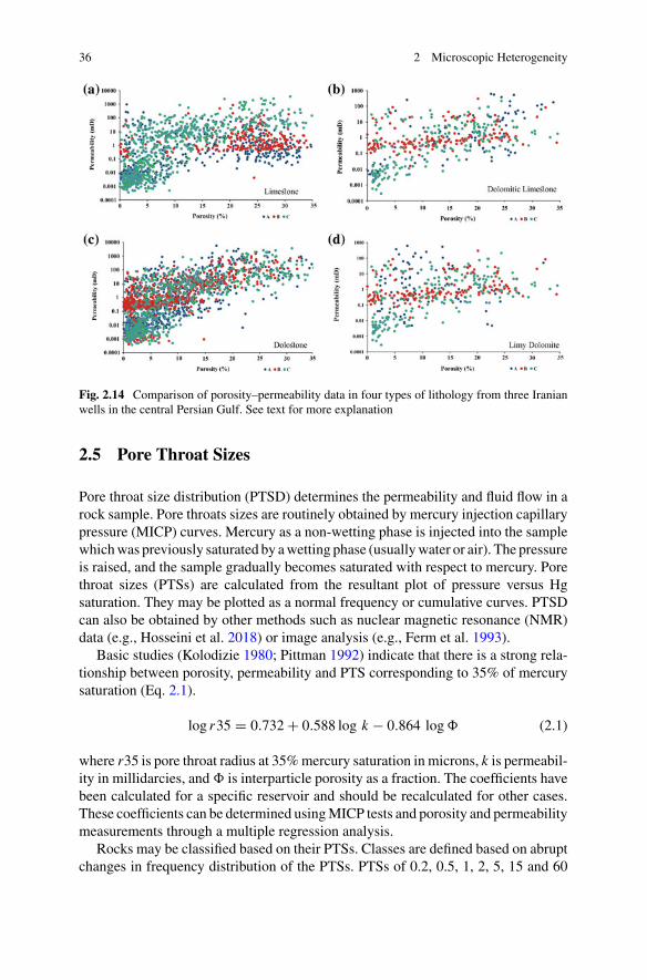
36 2 Microscopic Heterogeneity
Fig. 2.14 Comparison of porosity–permeability data in four types of lithology from three Iranianwells in the central Persian Gulf. See text for more explanation
2.5 Pore Throat Sizes
Pore throat size distribution (PTSD) determines the permeability and fluid flow in arock sample. Pore throats sizes are routinely obtained by mercury injection capillarypressure (MICP) curves. Mercury as a non-wetting phase is injected into the samplewhichwas previously saturated by awetting phase (usuallywater or air). The pressureis raised, and the sample gradually becomes saturated with respect to mercury. Porethroat sizes (PTSs) are calculated from the resultant plot of pressure versus Hgsaturation. They may be plotted as a normal frequency or cumulative curves. PTSDcan also be obtained by other methods such as nuclear magnetic resonance (NMR)data (e.g., Hosseini et al. 2018) or image analysis (e.g., Ferm et al. 1993).
Basic studies (Kolodizie 1980; Pittman 1992) indicate that there is a strong rela-tionship between porosity, permeability and PTS corresponding to 35% of mercurysaturation (Eq. 2.1).
log r35 = 0.732+ 0.588 log k − 0.864 log� (2.1)
where r35 is pore throat radius at 35%mercury saturation in microns, k is permeabil-ity in millidarcies, and � is interparticle porosity as a fraction. The coefficients havebeen calculated for a specific reservoir and should be recalculated for other cases.These coefficients can be determined usingMICP tests and porosity and permeabilitymeasurements through a multiple regression analysis.
Rocks may be classified based on their PTSs. Classes are defined based on abruptchanges in frequency distribution of the PTSs. PTSs of 0.2, 0.5, 1, 2, 5, 15 and 60
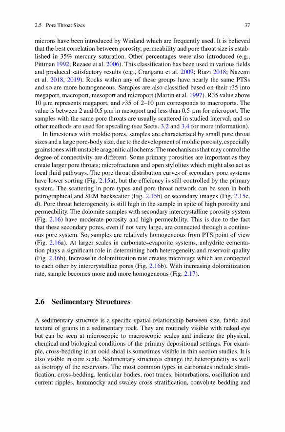
2.5 Pore Throat Sizes 37
microns have been introduced by Winland which are frequently used. It is believedthat the best correlation between porosity, permeability and pore throat size is estab-lished in 35% mercury saturation. Other percentages were also introduced (e.g.,Pittman 1992; Rezaee et al. 2006). This classification has been used in various fieldsand produced satisfactory results (e.g., Cranganu et al. 2009; Riazi 2018; Nazemiet al. 2018, 2019). Rocks within any of these groups have nearly the same PTSsand so are more homogeneous. Samples are also classified based on their r35 intomegaport, macroport, mesoport and microport (Martin et al. 1997). R35 value above10 µm represents megaport, and r35 of 2–10 µm corresponds to macroports. Thevalue is between 2 and 0.5 µm in mesoport and less than 0.5 µm for microport. Thesamples with the same pore throats are usually scattered in studied interval, and soother methods are used for upscaling (see Sects. 3.2 and 3.4 for more information).
In limestones with moldic pores, samples are characterized by small pore throatsizes and a large pore-body size, due to the development ofmoldic porosity, especiallygrainstoneswith unstable aragonitic allochems. Themechanisms thatmay control thedegree of connectivity are different. Some primary porosities are important as theycreate larger pore throats; microfractures and open stylolites which might also act aslocal fluid pathways. The pore throat distribution curves of secondary pore systemshave lower sorting (Fig. 2.15a), but the efficiency is still controlled by the primarysystem. The scattering in pore types and pore throat network can be seen in bothpetrographical and SEM backscatter (Fig. 2.15b) or secondary images (Fig. 2.15c,d). Pore throat heterogeneity is still high in the sample in spite of high porosity andpermeability. The dolomite samples with secondary intercrystalline porosity system(Fig. 2.16) have moderate porosity and high permeability. This is due to the factthat these secondary pores, even if not very large, are connected through a continu-ous pore system. So, samples are relatively homogeneous from PTS point of view(Fig. 2.16a). At larger scales in carbonate–evaporite systems, anhydrite cementa-tion plays a significant role in determining both heterogeneity and reservoir quality(Fig. 2.16b). Increase in dolomitization rate creates microvugs which are connectedto each other by intercrystalline pores (Fig. 2.16b). With increasing dolomitizationrate, sample becomes more and more homogeneous (Fig. 2.17).
2.6 Sedimentary Structures
A sedimentary structure is a specific spatial relationship between size, fabric andtexture of grains in a sedimentary rock. They are routinely visible with naked eyebut can be seen at microscopic to macroscopic scales and indicate the physical,chemical and biological conditions of the primary depositional settings. For exam-ple, cross-bedding in an ooid shoal is sometimes visible in thin section studies. It isalso visible in core scale. Sedimentary structures change the heterogeneity as wellas isotropy of the reservoirs. The most common types in carbonates include strati-fication, cross-bedding, lenticular bodies, root traces, bioturbations, oscillation andcurrent ripples, hummocky and swaley cross-stratification, convolute bedding and
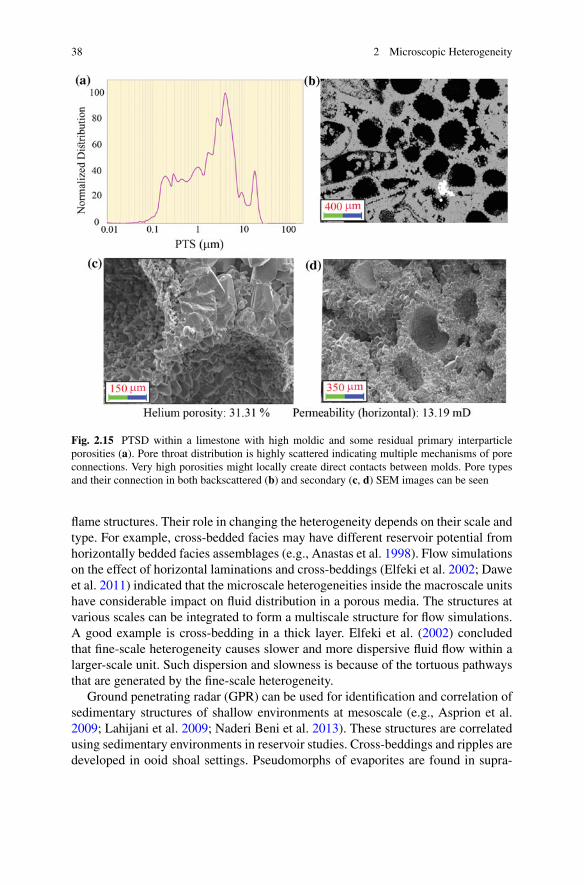
38 2 Microscopic Heterogeneity
Fig. 2.15 PTSD within a limestone with high moldic and some residual primary interparticleporosities (a). Pore throat distribution is highly scattered indicating multiple mechanisms of poreconnections. Very high porosities might locally create direct contacts between molds. Pore typesand their connection in both backscattered (b) and secondary (c, d) SEM images can be seen
flame structures. Their role in changing the heterogeneity depends on their scale andtype. For example, cross-bedded facies may have different reservoir potential fromhorizontally bedded facies assemblages (e.g., Anastas et al. 1998). Flow simulationson the effect of horizontal laminations and cross-beddings (Elfeki et al. 2002; Daweet al. 2011) indicated that the microscale heterogeneities inside the macroscale unitshave considerable impact on fluid distribution in a porous media. The structures atvarious scales can be integrated to form a multiscale structure for flow simulations.A good example is cross-bedding in a thick layer. Elfeki et al. (2002) concludedthat fine-scale heterogeneity causes slower and more dispersive fluid flow within alarger-scale unit. Such dispersion and slowness is because of the tortuous pathwaysthat are generated by the fine-scale heterogeneity.
Ground penetrating radar (GPR) can be used for identification and correlation ofsedimentary structures of shallow environments at mesoscale (e.g., Asprion et al.2009; Lahijani et al. 2009; Naderi Beni et al. 2013). These structures are correlatedusing sedimentary environments in reservoir studies. Cross-beddings and ripples aredeveloped in ooid shoal settings. Pseudomorphs of evaporites are found in supra-
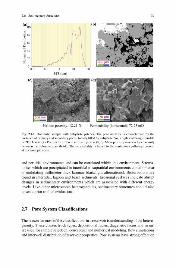
2.6 Sedimentary Structures 39
Fig. 2.16 Dolomitic sample with anhydrite patches. The pore network is characterized by thepresence of primary and secondary pores, locally filled by anhydrite. So, a high scattering is visiblein PTSD curve (a). Pores with different sizes are present (b, c).Microporosity was developedmainlybetween the dolomite crystals (d). The permeability is linked to the continuous pathways presentat microscopic scale
and peritidal environments and can be correlated within this environment. Stroma-tolites which are precipitated in intertidal to supratidal environments contain planaror undulating millimeter-thick laminae (dark/light alternations). Bioturbations arefound in intertidal, lagoon and basin sediments. Erosional surfaces indicate abruptchanges in sedimentary environments which are associated with different energylevels. Like other microscopic heterogeneities, sedimentary structures should alsoupscale prior to final evaluations.
2.7 Pore System Classifications
The reason formost of the classifications in a reservoir is understanding of the hetero-geneity. These classes (rock types, depositional facies, diagenetic facies and so on)are used for sample selection, conceptual and numerical modeling, flow simulationsand interwell distribution of reservoir properties. Pore systems have strong effect on

40 2 Microscopic Heterogeneity
Fig. 2.17 Dolomite with anhydrite patches with low PTS scattering (a). The pore system is madeup by intercrystalline pores and microvugs (b, c). The median pore size is low, but the permeabilityis high in the less cemented areas. Pores are connected via intercrystalline pores (d)
final reservoir properties. In fact, they control the fluid behavior (both storage andflow) and so rocks with the same pore systems exhibit the same behavior in a car-bonate reservoir. In contrast to sandstones, carbonates usually have complicated anddiverse pore systems. The proper choice of classification is one of the most importantsteps in heterogeneity evaluation of a reservoirs. An ideal pore system classificationshould also correlate to the facies classification system. This is performed in order topredict the pore types based on facies distribution in conceptual or numerical reser-voir models. Facies models are representative of the reservoir geometry, and theirdistribution indicates the spatial dimension of the reservoir. So, pore types can alsobe predicted if they assign to a specific facies.
The Archie classification (Archie 1952) of pore types is one of the preliminaryworks in this field. Archie believed that a pore system classification should honor theabsolute and relative permeability, capillary pressure and resistivity of the sample,rather than pore genesis and origin. He also tried to generalize his classification inorder to be applicable for wellsite and field petroleum geologists. Archie explainedthat using these general terms, the difference between geologists’ ideas about asample will beminimum and so collected data by different experts may be compared.

2.7 Pore System Classifications 41
The classification also includes another category for the textures of the matrix whichis not the subject of this book. His classification is as follows:
Class A: The dominant pore sizes are less than 0.01 mm. They are not visible underthe microscope.Class B: Pore spaces are visible with naked eye. They are larger than 0.01 but smallerthan 0.1 mm.Class C: Visible porosities with larger than 0.1 mm and smaller than size of cuttingswhich is about 2 mm.Class D: Porosities are larger than cutting size. They include vugs and large molds.
He also introduced excellent, good, fair and poor classes for 20, 15, 10 and 5%porosity in the samples, respectively. There are also some sampleswhich are assignedto two classes (such as B/Cwhen some large porosities are also visible, other than thefine pores). The Archie classification of pore system is still used, but with increas-ing the core samples, a large volume of data from thin section studies and newlydeveloped classifications, it is not used in many cases. The advantages of Archieclassification are that it can be easily applied without the need to any equipment andfast determination of the classes. Usually, size of the pores shows their formationmechanism and so classifying the samples based on their pore sizes indicates theirorigin. The large pores in classes C and D are secondary in origin, while class Bhas generally primary interparticle porosities. Intercrystalline pores are not visiblein many cases and so they fall into class A. Disadvantages include generalizationand lack of any indication of the porosity and permeability relationships. Micro- andintercrystalline porosities are not visible with naked eye and so they are not includedin this classification. Details of the pore systems, their connection and origin are notclearly visible on hand specimens.
The most well-known pore type classification was presented by Choquette andPray (1970). Their terms for various types of pores (Fig. 2.18) are applied in bothacademic studies and industrial projects. The main idea of this classification is therelationship between rock fabric and pore types. Pores are classified into three groupsincluding fabric-selective, not fabric-selective and fabric-selective or not. Here, thefabric selectivity is relationship between the pores and solid depositional and diage-netic constituents of the rocks. For example, ooids are formed in primary depositionalsettings. Interparticle porosities are developed between these grains. This is a fabric-selective porosity. Calcite or anhydrite cements fill the interparticle spaces, and thenooids are dissolved in meteoric diagenetic environment. The result of this process isformation of moldic porosities. These are also fabric-selective pores because theirshape and size follow themorphology of the primary constituents. In contrast, fractur-ing crosscuts all primary and diagenetic constituents and so it is not fabric-selective.The fabric-selective or not group may or may not follow the primary fabric of thesample. For example, burrows and borings may pass just through the rock matrix andnot the grains. Both rock matrix and grains may be affected by boring organisms. Sothey may belong to each groups. Such porosities are called fabric-selective or not.
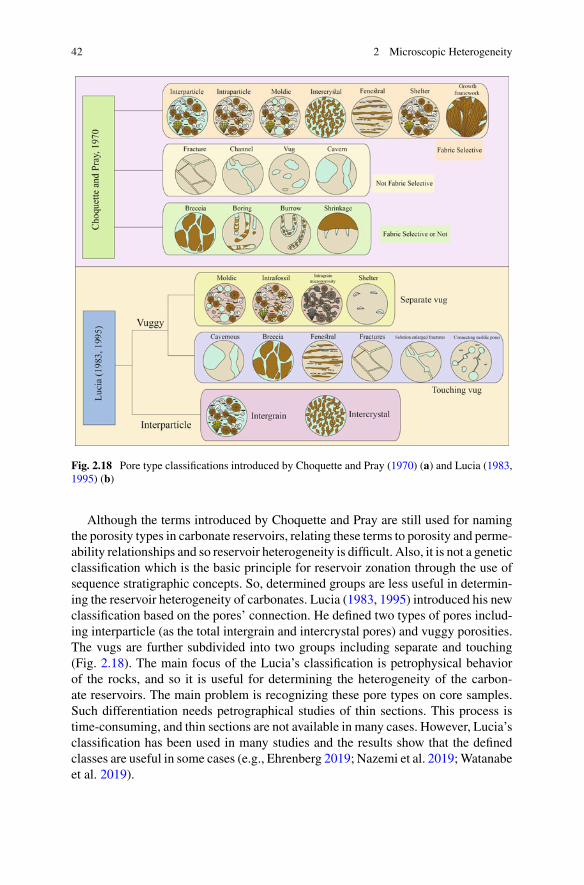
42 2 Microscopic Heterogeneity
Fig. 2.18 Pore type classifications introduced by Choquette and Pray (1970) (a) and Lucia (1983,1995) (b)
Although the terms introduced by Choquette and Pray are still used for namingthe porosity types in carbonate reservoirs, relating these terms to porosity and perme-ability relationships and so reservoir heterogeneity is difficult. Also, it is not a geneticclassification which is the basic principle for reservoir zonation through the use ofsequence stratigraphic concepts. So, determined groups are less useful in determin-ing the reservoir heterogeneity of carbonates. Lucia (1983, 1995) introduced his newclassification based on the pores’ connection. He defined two types of pores includ-ing interparticle (as the total intergrain and intercrystal pores) and vuggy porosities.The vugs are further subdivided into two groups including separate and touching(Fig. 2.18). The main focus of the Lucia’s classification is petrophysical behaviorof the rocks, and so it is useful for determining the heterogeneity of the carbon-ate reservoirs. The main problem is recognizing these pore types on core samples.Such differentiation needs petrographical studies of thin sections. This process istime-consuming, and thin sections are not available in many cases. However, Lucia’sclassification has been used in many studies and the results show that the definedclasses are useful in some cases (e.g., Ehrenberg 2019; Nazemi et al. 2019;Watanabeet al. 2019).
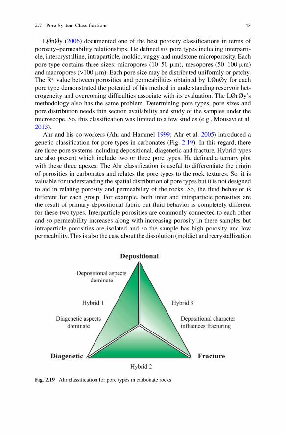
2.7 Pore System Classifications 43
LØnØy (2006) documented one of the best porosity classifications in terms ofporosity–permeability relationships. He defined six pore types including interparti-cle, intercrystalline, intraparticle, moldic, vuggy and mudstone microporosity. Eachpore type contains three sizes: micropores (10–50 µm), mesopores (50–100 µm)and macropores (>100 µm). Each pore size may be distributed uniformly or patchy.The R2 value between porosities and permeabilities obtained by LØnØy for eachpore type demonstrated the potential of his method in understanding reservoir het-erogeneity and overcoming difficulties associate with its evaluation. The LØnØy’smethodology also has the same problem. Determining pore types, pore sizes andpore distribution needs thin section availability and study of the samples under themicroscope. So, this classification was limited to a few studies (e.g., Mousavi et al.2013).
Ahr and his co-workers (Ahr and Hammel 1999; Ahr et al. 2005) introduced agenetic classification for pore types in carbonates (Fig. 2.19). In this regard, thereare three pore systems including depositional, diagenetic and fracture. Hybrid typesare also present which include two or three pore types. He defined a ternary plotwith these three apexes. The Ahr classification is useful to differentiate the originof porosities in carbonates and relates the pore types to the rock textures. So, it isvaluable for understanding the spatial distribution of pore types but it is not designedto aid in relating porosity and permeability of the rocks. So, the fluid behavior isdifferent for each group. For example, both inter and intraparticle porosities arethe result of primary depositional fabric but fluid behavior is completely differentfor these two types. Interparticle porosities are commonly connected to each otherand so permeability increases along with increasing porosity in these samples butintraparticle porosities are isolated and so the sample has high porosity and lowpermeability. This is also the case about the dissolution (moldic) and recrystallization
Fig. 2.19 Ahr classification for pore types in carbonate rocks
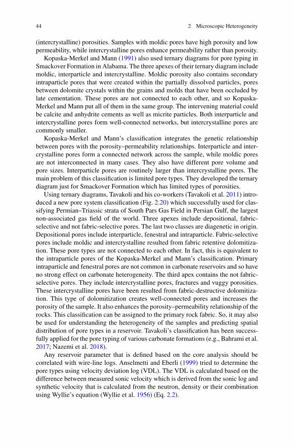
44 2 Microscopic Heterogeneity
(intercrystalline) porosities. Samples with moldic pores have high porosity and lowpermeability, while intercrystalline pores enhance permeability rather than porosity.
Kopaska-Merkel and Mann (1991) also used ternary diagrams for pore typing inSmackover Formation in Alabama. The three apexes of their ternary diagram includemoldic, interparticle and intercrystalline. Moldic porosity also contains secondaryintraparticle pores that were created within the partially dissolved particles, poresbetween dolomite crystals within the grains and molds that have been occluded bylate cementation. These pores are not connected to each other, and so Kopaska-Merkel and Mann put all of them in the same group. The intervening material couldbe calcite and anhydrite cements as well as micrite particles. Both interparticle andintercrystalline pores form well-connected networks, but intercrystalline pores arecommonly smaller.
Kopaska-Merkel and Mann’s classification integrates the genetic relationshipbetween pores with the porosity–permeability relationships. Interparticle and inter-crystalline pores form a connected network across the sample, while moldic poresare not interconnected in many cases. They also have different pore volume andpore sizes. Interparticle pores are routinely larger than intercrystalline pores. Themain problem of this classification is limited pore types. They developed the ternarydiagram just for Smackover Formation which has limited types of porosities.
Using ternary diagrams, Tavakoli and his co-workers (Tavakoli et al. 2011) intro-duced a new pore system classification (Fig. 2.20) which successfully used for clas-sifying Permian–Triassic strata of South Pars Gas Field in Persian Gulf, the largestnon-associated gas field of the world. Three apexes include depositional, fabric-selective and not fabric-selective pores. The last two classes are diagenetic in origin.Depositional pores include interparticle, fenestral and intraparticle. Fabric-selectivepores include moldic and intercrystalline resulted from fabric retentive dolomitiza-tion. These pore types are not connected to each other. In fact, this is equivalent tothe intraparticle pores of the Kopaska-Merkel and Mann’s classification. Primaryintraparticle and fenestral pores are not common in carbonate reservoirs and so haveno strong effect on carbonate heterogeneity. The third apex contains the not fabric-selective pores. They include intercrystalline pores, fractures and vuggy porosities.These intercrystalline pores have been resulted from fabric-destructive dolomitiza-tion. This type of dolomitization creates well-connected pores and increases theporosity of the sample. It also enhances the porosity–permeability relationship of therocks. This classification can be assigned to the primary rock fabric. So, it may alsobe used for understanding the heterogeneity of the samples and predicting spatialdistribution of pore types in a reservoir. Tavakoli’s classification has been success-fully applied for the pore typing of various carbonate formations (e.g., Bahrami et al.2017; Nazemi et al. 2018).
Any reservoir parameter that is defined based on the core analysis should becorrelated with wire-line logs. Anselmetti and Eberli (1999) tried to determine thepore types using velocity deviation log (VDL). The VDL is calculated based on thedifference between measured sonic velocity which is derived from the sonic log andsynthetic velocity that is calculated from the neutron, density or their combinationusing Wyllie’s equation (Wyllie et al. 1956) (Eq. 2.2).
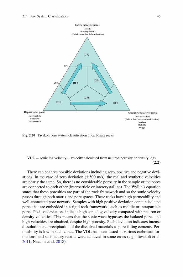
2.7 Pore System Classifications 45
Fig. 2.20 Tavakoli pore system classification of carbonate rocks
VDL = sonic log velocity− velocity calculated from neutron porosity or density logs(2.2)
There can be three possible deviations including zero, positive and negative devi-ations. In the case of zero deviation (±500 m/s), the real and synthetic velocitiesare nearly the same. So, there is no considerable porosity in the sample or the poresare connected to each other (interparticle or intercrystalline). The Wyllie’s equationstates that these porosities are part of the rock framework and so the sonic velocitypasses through both matrix and pore spaces. These rocks have high permeability andwell-connected pore network. Samples with high positive deviation contain isolatedpores that are embedded in a rigid rock framework, such as moldic or intraparticlepores. Positive deviations indicate high sonic log velocity compared with neutron ordensity velocities. This means that the sonic wave bypasses the isolated pores andhigh velocities are obtained, despite high porosity. Such deviation indicates intensedissolution and precipitation of the dissolved materials as pore-filling cements. Per-meability is low in such zones. The VDL has been tested in various carbonate for-mations, and satisfactory results were achieved in some cases (e.g., Tavakoli et al.2011; Nazemi et al. 2018).

46 2 Microscopic Heterogeneity
2.8 Rock Typing
Rock types (RT) are reservoir samples with the same petrophysical behavior. Theproperties of interest in a RT are fluid-related characteristics (Bear 1972; Tiab andDonaldson 2015; Tavakoli 2018). Like other classifying methods in the reservoir,RTs are also determined to overcome the heterogeneity challenges of the reservoir.In fact, all other methods such as diagenetic facies, rock fabric classes and electro-facies (see Sect. 2.9) try to define a proper RT with various points of view. Variousmethods have been developed to define a representative RT in a reservoir. Thesemethods have been used, explained, classified and interpreted previously (Tiab andDonaldson 2015; Tavakoli 2018). The flow unit (FU) also has the same concept withlarger scale. In fact, while RT is defined for each sample, a flow unit is defined tointegrate these microscale characteristics into a larger scale which can be correlatedthrough the reservoir. Table 2.1 shows the commonly used rock typing and flow unitdetermination methods, their necessary data and a brief description of each process.RTs, FUs and electrofacies use various data types but can be related to each other ina meaningful way (Fig. 2.21).
Table 2.1 Various rock typing and flow unit definition methods in carbonate reservoirs
Name Used data Methodology
Geological rock typing(GRT)
Facies and diagenesis datafrom thin sections andmacroscopic coredescriptions
Samples with the samegeological and petrophysicalproperties are defined
Winland r35 Porosity, permeability andpore throat size in 35% ofmercury saturation in MICPtest
Samples are classified basedon the same effective porethroats
Lucia rock fabric number Interparticle porosity andpermeability
Samples with the samepetrophysical classes andsimilar grain sizes aregrouped
Reservoir quality index (RQI)and flow zone indicator (FZI)
Porosity and permeability Samples with the samepermeability to porosity ratioare classified in the samegroups
Lorenz plot Porosity and permeability Zones are characterizedbased on deviations fromperfect equality line
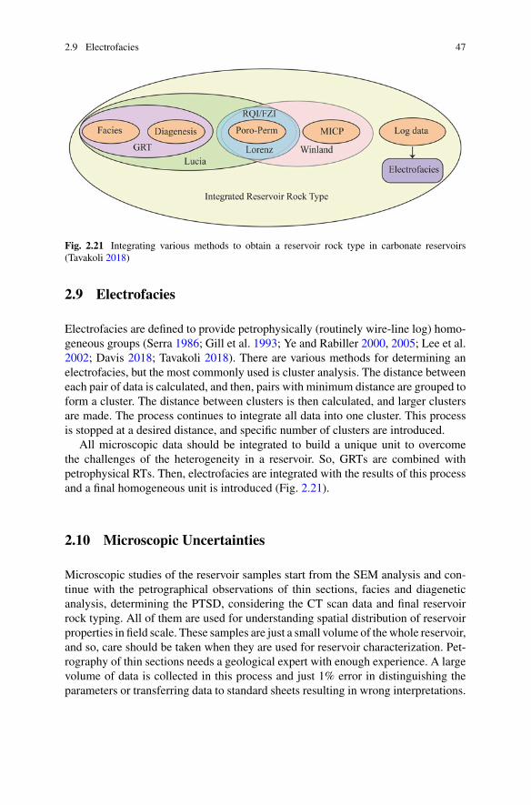
2.9 Electrofacies 47
Fig. 2.21 Integrating various methods to obtain a reservoir rock type in carbonate reservoirs(Tavakoli 2018)
2.9 Electrofacies
Electrofacies are defined to provide petrophysically (routinely wire-line log) homo-geneous groups (Serra 1986; Gill et al. 1993; Ye and Rabiller 2000, 2005; Lee et al.2002; Davis 2018; Tavakoli 2018). There are various methods for determining anelectrofacies, but the most commonly used is cluster analysis. The distance betweeneach pair of data is calculated, and then, pairs with minimum distance are grouped toform a cluster. The distance between clusters is then calculated, and larger clustersare made. The process continues to integrate all data into one cluster. This processis stopped at a desired distance, and specific number of clusters are introduced.
All microscopic data should be integrated to build a unique unit to overcomethe challenges of the heterogeneity in a reservoir. So, GRTs are combined withpetrophysical RTs. Then, electrofacies are integrated with the results of this processand a final homogeneous unit is introduced (Fig. 2.21).
2.10 Microscopic Uncertainties
Microscopic studies of the reservoir samples start from the SEM analysis and con-tinue with the petrographical observations of thin sections, facies and diageneticanalysis, determining the PTSD, considering the CT scan data and final reservoirrock typing. All of them are used for understanding spatial distribution of reservoirproperties in field scale. These samples are just a small volume of thewhole reservoir,and so, care should be taken when they are used for reservoir characterization. Pet-rography of thin sections needs a geological expert with enough experience. A largevolume of data is collected in this process and just 1% error in distinguishing theparameters or transferring data to standard sheets resulting in wrong interpretations.
48 2 Microscopic Heterogeneity
Determining the primary facies and diagenetic facies groups is a qualitative and com-plicated process which in part depends on the geologist’s experience and idea. Thereare various methods for defining a diagenetic facies, as discussed before. CT scanimages are taken with various resolution and spacing. These parameters stronglyaffect the final interpretations and even calculations. Allochems and porosities couldbe larger or smaller than the CT image resolution and spacing. The differentiationof the components strongly depends on their density and is presented as grayscalebetween 0 and 255. So, extracting the rock constituents is not easy. Pore systems havestrong effect on reservoir heterogeneity and predicting other reservoir parameters ina 3D space. Various methods can be used to classify the pore types of a reservoir;each of them has its special point of view. Selection of the most suitable methodbased on the properties of the studied reservoir is very important. Various logs maybe integrated to build a set of electrofacies. Log selection depends on the data cor-relation and the purpose of the study, which are different case by case. The finalmethod for compiling all microscopic units is also a complex procedure. Combininggeological and petrophysical data with a suitable method for rock typing are the mostchallenging part of any reservoir evaluation, especially carbonates. This challengecan be solved with the incorporation of all disciplines and use of quantitative data,as much as possible.
References
Abdolmaleki J, Tavakoli V, Asadi-Eskandar A (2016) Sedimentological and diagenetic controls onreservoir properties in the Permian-Triassic successions of Western Persian Gulf, Southern Iran.J Pet Sci Eng 141:90–113
Adam A, Swennen R, Abdulghani W, Abdlmutalib A, Hariri M, Abdulraheem A (2018) Reservoirheterogeneity and quality of Khuff carbonates in outcrops of central Saudi Arabia. Mar Pet Geol89:721–751
Ahr WM, Hammel B (1999) Identification and mapping of flow units in carbonate reservoirs:an example from Happy Spraberry (Permian) Field, Garza County, Texas USA. Energy ExplorExploit 17:311–334
AhrWM, Allen D, Boyd A, Bachman HN, Smithson T, Clerke EA, Gzara KBM, Hassall JK, MurtyCRK, Zubari H, Ramamoorthy R (2005) Confronting the carbonate conundrum. SchlumbergerOil field Rev 1:18–29
Anastas AS, James NP, Nelson CS, Dalrymple RW (1998) Deposition and textural evolution ofcool-water limestones: outcrop analog for reservoir potential in cross-bedded calcitic reservoirs.AAPG Bull 82:160–180
Anselmetti FS, Eberli GP (1999) The velocity-deviation log: a tool to predict pore type and per-meability trends in carbonate drill holes from sonic and porosity or density logs. AAPG Bull83:450–466
Archie GE (1952) Classification of carbonate reservoir rocks and petrophysical considerations.AAPG Bull 36(2):278–298
Asprion U, Westphal H, Nieman M, Pomar L (2009) Extrapolation of depositional geometries ofthe Menorcan Miocene carbonate ramp with ground-penetrating radar. Facies 55:37–46
Bahrami F, Moussavi-Harami R, Khanehbad M, Gharaie MM, Sadeghi R (2017) Identification ofpore types and pore facies for evaluating the diagenetic performance on reservoir quality: a casestudy from the Asmari Formation in Ramin Oil Field, SW Iran. Geosci J 21:565–577
References 49
Bear J (1972) Dynamics of fluids in porous media. American Elsevier Publishing Co., New YorkBruna PO, Lavenu APC, Matonti C, Bertotti G (2019) Are stylolites fluid-flow efficient features? JStruct Geol 125:270–277
Carnell AJH, Wilson MEJ (2004) Dolomites in SE Asia–varied origins and implications forhydrocarbon exploration. Geol Soc Lond Spec Publ 235:255–300
Choquette PW, Pray LC (1970) Geologic nomenclature and classification of porosity in sedimentarycarbonates. AAPG Bull 54(2):207–250
Cranganu C, Villa MA, Saramet M, Zakharova N (2009) Petrophysical characteristics of sourceand reservoir rocks in the Histria basin, western Black Sea. J Pet Geol 32:357–372
Cui Y, Wang G, Jones SJ, Zhou Z, Ran Y, Lai J, Li R, Deng L (2017) Prediction of diagenetic faciesusing well logs—a case study from the upper Triassic Yanchang Formation, Ordos Basin, China.Mar Pet Geol 81:50–65
Davis JC (2018) Electrofacies in reservoir characterization. In: Daya Sagar B, Cheng Q, AgterbergF (eds) Handbook of mathematical geosciences. Springer, Cham
DaweRA, CaruanaA, Grattoni CA (2011) Immiscible displacement in cross-bedded heterogeneousporous media. Transp Porous Med 87:335–353
Dunham RJ (1962) Classification of carbonate rocks according to depositional texture. In: HamWE (ed) Classification of carbonate rocks. AAPG Memoir 1, Oklahoma
Ehrenberg SN (2019) Petrophysical heterogeneity in a lower cretaceous limestone reservoir, onshoreAbu Dhabi, United Arab Emirates. AAPG Bull 103:527–546
Ehrenberg SN, Nadeau PH (2005) Sandstone vs. carbonate petroleum reservoirs: a globalperspective on porosity-depth and porosity-permeability relationships. AAPG Bull 89:435–445
Ehrenberg SN,WalderhaugO (2015) Preferential calcite cementation ofmacropores inmicroporouslimestones. J Sediment Res 85:780–793
Elfeki AM, Dekking FM, Bruining J, Kraaikamp C (2002) Influence of fine-scale heterogeneitypatterns on large-scale behavior of miscible transport in porous media. Pet Geosci 8:159–165
Embry AF, Klovan JE (1971) A Late Devonian reef tract on Northeastern Banks Island, NWT. CanPetro Geol Bull 19:730–781
Ferm JB, Ehrlich R, Crawford GA (1993) Petrographic image analysis and petrophysics: analysisof crystalline carbonates from the Permian basin, west Texas. Carbonates Evaporites 8:90–108
Flugel E (2010) Microfacies of carbonate rocks, analysis, interpretation and application. Springer,Berlin
Friedman GM (1965) Terminology of crystallization textures and fabrics in sedimentary rocks. JSediment Pet 35:643–655
Gill D, ShomronyA, FligelmanH (1993) Numerical zonation of log suites and logfacies recognitionby multivariate clustering. AAPG Bull 77:1781–1791
Gressly A (1838) Observations géologiques sur le Jura soleurois, vol 1. Imprimerie de Petitpierre(in French)
Hashim MS, Kaczmarek SE (2019) A review of the nature and origin of limestone microporosity.Mar Pet Geol 107:527–554
Hosseini M, Tavakoli V, Nazemi M (2018) The effect of heterogeneity on NMR derived capillarypressure curves, case study of Dariyan tight carbonate reservoir in the central Persian Gulf. J PetSci Eng 171:1113–1122
Huang SJ, Huang KK, Lu J, Lan YF (2014) The relationship between dolomite textures and theirformation temperature: a case study from the Permian-Triassic of the Sichuan Basin and the lowerPaleozoic of the Tarim Basin. Pet Sci 11:39–51
Koehn D, Rood MP, Beaudoin N, Chung P, Bons PD, Gomez-Rivas E (2016) A new stylo-lite classification scheme to estimate compaction and local permeability variations. Sed Geol346:60–71
Kolodizie SJ (1980)Analysis of pore throat size and use of theWaxman-Smits equation to determineOOIP in Spindle Field, Colorado. SPE paper 9382 presented at the 1980 SPE annual technicalconference and exhibition, Dallas, Texas
50 2 Microscopic Heterogeneity
Kopaska-Merkel DC, Mann SD (1991) Pore facies of Smackover carbonate reservoirs in southwestAlabama. Gulf Coast Ass Geol Soc Trans 41:374–382
Lahijani HAK, Rahimpour-Bonab H, Tavakoli V, Hosseindoost M (2009) Evidence for lateHolocene highstands in Central Guilan-East Mazanderan, South Caspian coast, Iran. QuaternInt 197:55–71
Lai J, Fan X, Pang X, Zhang X, Xiao C, Zhao X, Han C, Wang G, Qin Z (2019) Correlatingdiagenetic facies with well logs (conventional and image) in sandstones: the Eocene-OligoceneSuweiyi Formation in Dina 2 Gasfield, Kuqa depression of China. J Pet Sci Eng 174:617–636
Lee SH, Kharghoria A, Datta-Gupta A (2002) Electrofacies characterization and permeabilitypredictions in complex reservoirs. SPE Reserv Eval Eng 5:237–248
LØnØy A (2006) Making sense of carbonate pore systems. AAPG Bull 90:1381–1405Lucia FJ (1983) Petrophysical parameters estimated from visual description of carbonate rocks: afield classification of carbonate pore space. J Pet Tech 35:626–637
Lucia FJ (1995) Rock fabric/petrophysical classification of carbonate pore space for reservoircharacterization. AAPG Bull 79:1275–1300
Lucia FJ, Major RP (1994) Porosity evolution through hypersaline reflux dolomitization. In: PurserB, Tucker M, Zenger D (eds) Dolomites: International Association of Sedimentologists SpecialPublications 21345–360
Machel HG (2004) Concepts and models of dolomitization—a critical reappraisal. In: BraithwaiteC, Rizzi G, Darke G (eds) The geometry and petrogenesis of dolomite hydrocarbon reservoirs.Geological Society, London, Special Publications 235:7–63
Martin AJ, Solomon ST, Hartmann DJ (1997) Characterization of petrophysical flow units incarbonate reservoirs. AAPG Bull 81:734–759
Mehrabi H, Mansouri M, Rahimpour-Bonab H, Tavakoli V, Hassanzadeh M (2016) Chemical com-paction features as potential barriers in the Permian-Triassic reservoirs of South Pars Field,Southern Iran. J Pet Sci Eng 145:95–113
MousaviM, ProdanovicM, Jacobi D (2013)New classification of carbonate rocks for process-basedpore-scale modeling. SPE J 18:243–263
Nader FH (2017) Multi-scale quantitative diagenesis and impacts on heterogeneity of carbonatereservoir rocks. Springer, Cham, Switzerland
Naderi Beni A, Lahijani H, Moussavi Harami R, Leroy SAG, Shah-Hosseini M, Kabiri K, TavakoliV (2013) Development of spit-lagoon complexes in response to Little Ice Age rapid sea-levelchanges in the central Guilan coast, South Caspian Sea, Iran. Geomorphology 187:11–26
Naderi-Khujin M, Seyrafian A, Vaziri-Moghaddam H, Tavakoli V (2016) Characterization of theLate Aptian top-Dariyan disconformity surface, offshore SW Iran: a multi-proxy approach. J PetGeol 39:269–286
Nazemi M, Tavakoli V, Rahimpour-Bonab H, Hosseini M, Sharifi-Yazdi M (2018) The effect ofcarbonate reservoir heterogeneity on Archie’s exponents (a and m), an example fromKangan andDalan gas formations in the central Persian Gulf. J Nat Gas Sci Eng 59:297–308
Nazemi M, Tavakoli V, Sharifi-Yazdi M, Rahimpour-Bonab H, Hosseini M (2019) The impact ofmicro-to macro-scale geological attributes on Archie’s exponents, an example from Permian-Triassic carbonate reservoirs of the central Persian Gulf. Mar Pet Geol 102:775–785
Pittman ED (1992) Relationship of porosity and permeability to various parameters derived frommercury injection-capillary pressure curves for sandstone. AAPG Bull 72:191–198
Purser BH, Brown A, Aissaoui DM (1994) Nature, origins and evolution of porosity in dolomite.In: Purser B, TuckerM, Zenger D (eds) Dolomites. International Association of SedimentologistsSpecial Publications 21:283–308
Rezaee MR, Jafari A, Kazemzadeh E (2006) Relationship between permeability, porosity and porethroat size in carbonate rocks using regression analysis and neural networks. J Geophys Eng3:370–376
Riazi Z (2018) Application of integrated rock typing and flow units identification methods for anIranian carbonate reservoir. J Pet Sci Eng 160:483–497
References 51
Sagan JA, Hart BS (2006) Three-dimensional seismic-based definition of fault-related porositydevelopment: Trenton-Black River interval, Saybrook, Ohio. AAPG Bull 90:1763–1785
Saller AH (2004) Palaeozoic dolomite reservoirs in the Permian Basin, SW USA: stratigraphicdistribution, porosity, permeability and production. Geol Soc Lond Spec Publ 235:309–323
Saller AH, Henderson N (1998) Distribution of porosity and permeability in platform dolomites:insight from the Permian of west Texas. AAPG Bull 82:1528–1550
Saller AH, Henderson N (2001) Distribution of porosity and permeability in platform dolomites:insight from the Permian of west Texas: reply. AAPG Bull 85:530–532
Serra O (1986) Fundamentals of well log interpretation, vol 2. The interpretation of logging data.Elsevier, Amsterdam
Sibley DF, Gregg JM (1987) Classification of dolomite rock textures. J Sed Pet 57:967–975Sun H, Vega S, Tao G (2017) Analysis of heterogeneity and permeability anisotropy in carbonaterock samples using digital rock physics. J Pet Sci Eng 156:419–429
Tavakoli V (2018) Geological core analysis: application to reservoir characterization. Springer,Cham, Switzerland
Tavakoli V, Jamalian A (2018) Microporosity evolution in Iranian reservoirs, Dalan and Dariyanformations, the central Persian Gulf. J Nat Gas Sci Eng 52:155–165
Tavakoli V, Naderi-Khujin M, Seyedmehdi Z (2018) The end-permian regression in the westerntethys: sedimentological and geochemical evidence fromoffshore the PersianGulf, Iran.Geo-MarLett 38(2):179–192
Tavakoli V, Jamalian A (2019) Porosity evolution in dolomitized Permian-Triassic strata of thePersian Gulf, insights into the porosity origin of dolomite reservoirs. J Pet Sci Eng 181:106191
Tavakoli V, Rahimpour-Bonab H, Esrafili-Dizaji B (2011) Diagenetic controlled reservoir qualityof South Pars gas field, an integrated approach. C R Geosci 343:55–71
Tiab D, Donaldson EC (2015) Petrophysics, theory and practice of measuring reservoir rock andfluid transport properties. Gulf Professional Publishing, Houston
Tucker M, Wright VP (1990) Carbonate sedimentology. Blackwell Scientific Publications, OxfordWang J, Cao Y, Liu K, Liu J, Kashif M (2017) Identification of sedimentary-diagenetic facies andreservoir porosity and permeability prediction: an example from the Eocene beach-bar sandstonein the Dongying Depression, China. Mar Pet Geol 82:69–84
Warren J (2000) Dolomite: occurrence, evolution and economically important associations. EarthSci Rev 52:1–81
Watanabe N, Kusanagi H, Shimazu T, Yagi M (2019) Local non-vuggy modeling and relationsamong porosity, permeability and preferential flow for vuggy carbonates. Eng Geol 248:197–206
WyllieMR, Gregory AR, Gardner GHF (1956) Elastic wave velocities in heterogeneous and porousmedia. Geophysics 21:41–70
Ye S, Rabiller P (2000) A new tool for electro-facies analysis: multi-resolution graph-basedclustering. In: SPWLA 41st annual logging symposium, Dallas, Texas, pp 14–27
Ye S, Rabiller P (2005) Automated electrofacies ordering. Petrophysics 46:409–423Zou C, Tao S, Zhou H, Zhang X, He D, Zhou C, Wang L, Wang X, Li F, Luo P, Yuan X (2008)Genesis, classification, and evaluation method of diagenetic facies. Pet Explor Dev 35:526–540
Chapter 3Mesoscopic Heterogeneity
Abstract Microscopic homogeneous unites which are defined based on the fine-scale data are combined to form larger-scale units. Facies are grouped together tocreate a facies group and facies belts. These groups are interpolated between thewells using the concept of facies models. These models are constructed by compar-ing various sedimentary environments from different parts of the world. They actas a template for comparison, future observations, distribution of geological prop-erties in space and time and also for understanding the primary physical, chemicaland biological conditions of the depositional settings. While facies, facies groupsand facies belts indicate the geological heterogeneity of the reservoir, hydraulic flowunits divide the intervals into homogeneous groups from petrophysical point of view.These units are defined using various methods which are still evolving. Petrophys-ical characteristics are integrated with facies models and properties are upscaledinto a coarser grid suitable for numerical reservoir modeling. The cyclicities of thefacies and properties indicate the periodicity of the primary depositional conditionswhich, in turn, are used for heterogeneity analysis of the strata. These cyclicities aredefined using sequences in most cases. Both geological (facies and diagenesis) andpetrophysical properties are correlated in the framework of sequence stratigraphicunits in the reservoir. Rocks between the boundaries of the sequences are geneticallyrelated and so have similar primary geological and petrophysical characteristics.With respect to these similarities, their diagenesis are also the same in most cases.So, defining facies, facies groups, facies models, hydraulic flow units and recogniz-able genetically related units at various scales helps to overcome the challenges ofheterogeneity in carbonate reservoirs.
3.1 Sedimentary Environments
Facies are the main building blocks of the reservoirs’ body from sedimentologicalpoint of view. Also, other reservoir characteristics such as diagenesis or petrophysi-cal parameters usually follow the primary facies of the rocks. So, understanding bothhorizontal and vertical facies distributions plays a fundamental role in any formation
© The Author(s), under exclusive license to Springer Nature Switzerland AG 2020V. Tavakoli, Carbonate Reservoir Heterogeneity,SpringerBriefs in Petroleum Geoscience & Engineering,https://doi.org/10.1007/978-3-030-34773-4_3
53
54 3 Mesoscopic Heterogeneity
evaluation. The concept of sedimentary environment as a media for sediment accu-mulation has been used for many years by sedimentologists. The spatial relationshipsbetween facies, their sequence and resulting vertical accumulation were first intro-duced by (Walker 1984). He stated that the facies and sedimentary environmentswhich are observed beside each other are superimposed during the transgressionand regression cycles. This means that two consecutive facies in a vertical columnbelong to two adjacent sedimentary environments. Although the law should be usedwith care, it provides the basis for reconstructing sedimentary environments and spa-tial distribution of the facies based on their sedimentary environments. It is worthmentioning that erosional surfaces or any other discontinuity in the rock record dis-turb this relationship. A facies model (Walker 1984) is representing the relationshipsbetween facies and combining them based on the concept of sedimentary environ-ments. Facies models can be presented by a sequence of facies, conceptual models,block diagrams and graphs. The concept of facies model, which is usually expressedas sedimentary environments, is used to predict the spatial properties of the reser-voir rocks, at least from the sedimentary point of view. As mentioned, many otherproperties follow this distribution. The introduction of the facies models is one ofthe main revolutions in the science of petroleum geology.
There are four important functions for a facies model (Walker 1984) including(1) it is used for purposes of comparison. This means that any facies model must actas a template or standard. Any sequence of facies is compared with a standard faciesmodel and so follows its geometry, reservoir properties and rock textures. A carbon-ate ramp is a good example. A sequence of peritidal mudstone, lagoonal wackestoneand some sparse ooid grainstones of the shoal without any evidence of a large andextensive barrier clearly indicates a ramp environment. Other evidence such as sharpchange in slope and sliding and slumping structures should also be present. Afterrecognizing the environment, the ramp template can be used for distributing theproperties. Other examples include low reservoir quality as well as blanket geom-etry in peritidal environments, mud-dominated microporous lagoon sediments andmeteoric dissolution in aragonitic ooids of the shoals. (2) It acts as a framework forfuture observations. A distinct facies model has known primary and secondary char-acteristics which can be used for other environments. (3) A facies model predicts thedistribution of geological properties in the reservoir. (4) It is used for interpretation ofthe primary physical, geochemical and biological conditions of the rocks. Regardingthese characteristics, a faciesmodel and its resulting sedimentary environment can beused for understanding and predicting the heterogeneity of a reservoir at mesoscale.
Defining a sedimentary environment enables the construction of both conceptualand numeric 3D facies models. Each sedimentary environment has its specific geom-etry, and so the spatial distributions of facies and the related petrophysical propertiesare understood. The result is a facies model which can be used for both quantitativeand qualitative evaluation of reservoir properties.
An important point in defining a faciesmodel and using it as a basis for reconstruct-ing the sedimentary environment as well as predicting reservoir properties is that thecarbonates are born, not made. They are born by living organisms, and as organismshave changed during the geological times, the nature of the carbonate facies and the
3.1 Sedimentary Environments 55
corresponding sedimentary environments also have been transformed during geo-logical periods. Epeiric ramps are good examples. These extensive shallow inlandseas have covered the continents during transgressive periods of sea level. The photiczone was very extensive, and so, a large area was covered by the carbonate factory.Wide facies belts were developed in these shallow seas. The subenvironments werehundreds of kilometers in length and width. The Permian–Triassic Dalan Formationequivalent to Khuff Formation in Oman, Bahrain, Saudi Arabia and Kuwait, ChiaZairi in Iraq and Bih and Hagil in United Arab Emirates has been deposited in suchenvironment. This formation hosts the largest gas reservoir of the world.
Defining the facies and determining a facies model or sedimentary environmentneeds geological core studies. Regarding the Walter’s law, a conceptual model canbe introduced by geological studies of at least one well core, but building a numerical3D model needs a reasonable number of cores in different wells of a field. Cores arenot available in many cases or at least are not enough to reconstruct such model. So,electrofacies concept (Sect. 2.9) is used instead. They are defined based on the wire-line logs which are routinely available from many wells. Unfortunately, standardfacies models are not available for these electrofacies at this time. In fact, defininga model for a petrophysical property which is controlled by many variables is notpossible in many cases. So, propagating the properties is based on the mathematicalformulas. These formulas ignore geological heterogeneities and so are not as reliableas real facies models in reservoir studies.
The first step for determining depositional sedimentary environment is faciescharacterization. Facies are grouped to form a facies group. A facies group is acombination of similar facies in terms of their depositional properties (Tavakoli2018). Facies groups, in turn, are combined to form a facies zone or belt using thesame conditions. For example, peloid wackestone, bioclast peloid wackestone andpeloid bioclast wackestone can be grouped into the peloid/bioclast wackestone faciesgroup. This facies group along with other groups such as fossiliferous mudstoneand peloid/bioclast packstone belong to lagoonal facies zone. These zones are con-stituents of a depositional environment. In this example, peritidal and lagoonal zonein combination with shoal and open marine facies zones forms a ramp depositionalsetting.
There are various types of carbonate environments, but few of them are suscepti-ble to petroleum accumulation. These aremarine shallow depositional settings whichare main carbonate-producing environments. They include shelves, ramps, platformsand atolls. There are two types of ramps including homoclinal and distally steepenedramps (Read 1982). Homoclinal ramps are extended from shallow nearshore settingto deep offshore basin without a major break. They have very gentle (usually lessthan 1 degree) depositional slope. Distally steepened ramps are characterized by adistinct break at the deep part of the ramp environment. Shelves include rimmed andnon-rimmed carbonates (Ginsburg and James 1974). Rimmed shelves are flat-toppedcarbonates with a rim in their outer ridge. This rim can be formed by reefs, shoals orislands. Non-rimmed carbonates have no effective rim in their morphology to absorbthe waves’ energy. So, they are similar to ramps with an incomplete barrier. Plat-forms include epeiric, isolated and drowned. Epeiric platforms (Shaw 1964) were
56 3 Mesoscopic Heterogeneity
characterized by very extensive shallow environments which has no counterpart inmodern depositional settings. Isolated platforms are detached shallow-water carbon-ates generally with steep margins into deep water. Almost all carbonate depositionalsettings may be drowned due to subsidence, rapid sea-level rise or change in carbon-ate productivity as the result of environmental stress. Oceanic atolls are formed byvolcanos rising hundreds of meters from the sea floor. The crest is close to the waterlevel, and the surrounding areas are covered by deep water.
Facies types in various depositional environments are limited and graduallychangewith increasing thewater depth. Flugel (2010) introduced the standardmicro-facies for both ramps and rimmed shelves. Sedimentary environments can be recon-structed based on the sequence of these facies usingWalter’s law. These environmentstransform to each other through time. Rapid sea-level rise cause drowning of the envi-ronment and rimmed shelves are converted to ramps. In contrast, sea-level fall causessubaerial exposure which also may change the environment. High siliciclastic inputsshut down the living organisms and cause major changes in the depositional set-tings. In geological time, plate movements change temperature, salinity and oceaniccurrents. These variations have strong effects on secreting organisms. The result ismajor changes in carbonate production in different parts of the environment.
3.2 Hydraulic Flow Units
Defining homogeneous units with respect to fluid flow and storage in carbonatereservoirs was the focus of many studies. Bear (1972) defined a hydraulic flow unit(HFU) as a volume with the same geological and petrophysical properties. Ebanks(1987) has the same definition, but he believed that such unit must be mappable at thereservoir scale. Hear et al. (1984) stated that this unit should be laterally continuous.Gunter et al. (1997) presented a same definition. Tiab and Donaldson (2015) statedthat anHFU is a geological/engineering unit that is defined to describe the storage andflow properties of the reservoir zones. Tavakoli (2018) concluded from the all abovedefinitions that a rock type and a flow unit are different in the scale of investigation. Infact, rock types are determined at the core scale, while HFUs are defined at reservoirscale. So, HFUs can be correlated between the wells.
Amaefule et al. (1993) introduced the ratio of permeability to effective porosity asa good indicator of HFUs. They defined the reservoir quality index (RQI) (Eq. 3.1)and flow zone indicator (FZI) (Eqs. 3.2 and 3.3) which were used in many studies toevaluate the heterogeneity of the reservoirs.
RQI (μm) = 0.0314 (K/�)0.5 (3.1)
FZI = RQI/�z (3.2)
�z = �/(1 − �) (3.3)
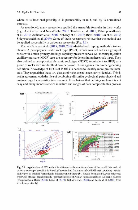
3.2 Hydraulic Flow Units 57
where � is fractional porosity, K is permeability in mD, and �z is normalizedporosity.
As mentioned, many researchers applied the Amaefule formulas in their works(e.g., Al-Dhafeeri and Nasr-El-Din 2007; Tavakoli et al. 2011; Rahimpour-Bonabet al. 2012; Arifianto et al. 2018; Nabawy et al. 2018; Riazi 2018; Liu et al. 2019;Soleymanzadeh et al. 2019). Some of these researchers believe that the method canbe applied successfully in carbonate reservoirs (Fig. 3.1).
Mirzaei-Paiaman et al. (2015, 2018, 2019) divided rock typing methods into twoclasses. A petrophysical static rock type (PSRT) which was defined as a group ofrocks with similar primary drainage capillary pressure curves. So, mercury injectioncapillary pressure (MICP) tests are necessary for determining these rock types. Theyalso defined a petrophysical dynamic rock type (PDRT) (equivalent to HFU) as agroup of rocks with similar fluid flow behavior. This is again a reservoir engineeringdefinition. Knowledge of HFUs of PDRTs is needed to identify more prolific inter-vals. They argued that these two classes of rocks are not necessarily identical. This isnot in agreement with the idea of combining all similar geological, petrophysical andengineering characteristics into one unit. It is obvious that defining such unit is noteasy and many inconsistencies in nature and ranges of data complicate this process
Fig. 3.1 Application of FZI method in different carbonate formations of the world. Normalizedporosity versus permeability in Sarvak (Cenomanian) formation inMiddleEast (a), porosity–perme-ability plot of Mishrif Formation in Missan oilfield (Iraq) (b), Rudeis Formation (Lower Miocene)fromGulf of Suez (c) andporosity–permeability plot ofAsmari Formation (Oligo–Miocene, Zagros)(compiled from Riazi (2018), Liu et al (2019), Nabawy et al. (2018) and Farshi et al. (2019) froma to d, respectively)

58 3 Mesoscopic Heterogeneity
but the ultimate goal is defining one unit which can be used in integrated static anddynamic numerical reservoir modeling.
FZI* or FZI-Star was introduced by Mirzaei-Paiaman et al. for determining theHFUs which is calculated based on the permeability–porosity ratio (Eq. 3.4) or usinga multiple linear regression equation form (Eq. 3.5). From their definition, it can beconcluded that FZI* and RQI of Amaefule are the same. They also believed that FZIis a function of grain size rather than pore throat size.
FZI∗ = RQI (μm) = 0.0314 (K/�)0.5 (3.4)
log(FZI∗
) = −1.50307 + 0.5log(K ) − 0.5log(�) (3.5)
Izadi andGhalambor (2013) defined two new indices includingmodified reservoirquality index (MRQI) (Eq. 3.6) and modified flow zone indicator (MFZI) based onthe Poiseuille and Darcy equations (Eq. 3.7) as follows:
MRQI = 0.0314 (K/�)0.5(1 − Swir)0.5 (3.6)
MFZI = MRQI/�z(1 − Swir)0.5 (3.7)
Although the Izadi and Ghalambor used the sandstone samples to obtain theirequations, Mirzaei-Paiaman et al. (2018) used their indices for Albian–CenomanianIlam and Sarvak carbonate reservoirs. It is worth mentioning that these methods needfurther verification by using new data from other regions. Nazari et al. (2019) appliedthe FZI*method to tight carbonates of Upper PermianDalan Formation in the centralPersian Gulf (Fig. 3.2). They concluded that the method differentiates tight samplesfrom other parts of the K3 reservoir unit in this formation.
3.3 Cyclicity
Repeated cycles of carbonate facies are deposited during geological time. This hier-archy is important because they are used for systematic division of strata. Under-standing causes and consequences of this hierarchy is also important because anordered forcing-mechanism is responsible for generation of these repetitions. Themain control on cyclicity of sediments is attributed to changes in accommodationwhich, in turn, is the result of climate variations.
The repetitions and cyclic pattern of changes is deduced from similarities insediments’ properties and stratal surfaces. These bounding surfaces should be corre-latable at regional scales. According to Lerat et al. (2000), the criterion for repetitionis the extent of changes within a cycle. So, minor cyclic changes create smaller scalecycles, while major changes in depositional setting form the larger cycles.
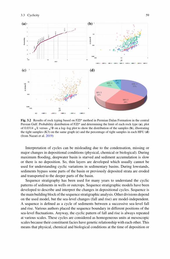
3.3 Cyclicity 59
Fig. 3.2 Results of rock typing based on FZI* method in Permian Dalan Formation in the centralPersian Gulf. Probability distribution of FZI* and determining the limit of each rock type (a), plotof 0.0314
√k versus
√� on a log–log plot to show the distribution of the samples (b), illustrating
the tight samples (K3) on the same graph (c) and the percentage of tight samples in each HFU (d)(from Nazari et al. 2019)
Interpretation of cycles can be misleading due to the condensation, missing ormajor changes in depositional conditions (physical, chemical or biological). Duringmaximum flooding, deepwater basin is starved and sediment accumulation is slowor there is no deposition. So, thin layers are developed which usually cannot beused for understanding cyclic variations in sedimentary basins. During lowstands,sediments bypass some parts of the basin or previously deposited strata are erodedand transported to the deeper parts of the basin.
Sequence stratigraphy has been used for many years to understand the cyclicpatterns of sediments in wells or outcrops. Sequence stratigraphic models have beendeveloped to describe and interpret the changes in depositional cycles. Sequence isthemain buildingblockof the sequence stratigraphic analysis.Other divisions dependon the used model, but the sea-level changes (fall and rise) are model-independent.A sequence is defined as a cycle of sediments between a successive sea-level falland rise. Various authors placed the sequence boundary in different positions of thesea-level fluctuations. Anyway, the cyclic pattern of fall and rise is always repeatedat various scales. These cycles are considered as homogeneous units at mesoscopicscales because their constituent facies have genetic relationship with each other. Thismeans that physical, chemical and biological conditions at the time of deposition or
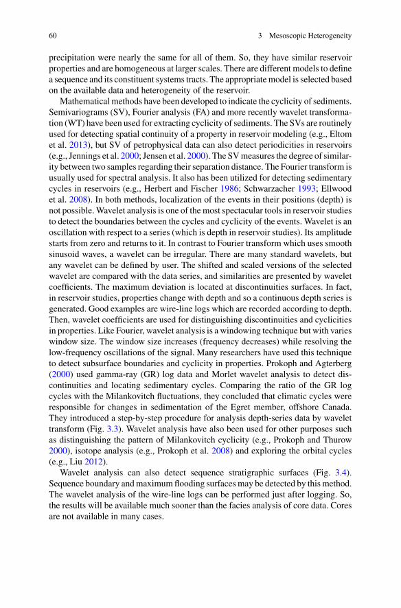
60 3 Mesoscopic Heterogeneity
precipitation were nearly the same for all of them. So, they have similar reservoirproperties and are homogeneous at larger scales. There are different models to definea sequence and its constituent systems tracts. The appropriatemodel is selected basedon the available data and heterogeneity of the reservoir.
Mathematical methods have been developed to indicate the cyclicity of sediments.Semivariograms (SV), Fourier analysis (FA) and more recently wavelet transforma-tion (WT) have been used for extracting cyclicity of sediments. The SVs are routinelyused for detecting spatial continuity of a property in reservoir modeling (e.g., Eltomet al. 2013), but SV of petrophysical data can also detect periodicities in reservoirs(e.g., Jennings et al. 2000; Jensen et al. 2000). The SVmeasures the degree of similar-ity between two samples regarding their separation distance. The Fourier transform isusually used for spectral analysis. It also has been utilized for detecting sedimentarycycles in reservoirs (e.g., Herbert and Fischer 1986; Schwarzacher 1993; Ellwoodet al. 2008). In both methods, localization of the events in their positions (depth) isnot possible.Wavelet analysis is one of the most spectacular tools in reservoir studiesto detect the boundaries between the cycles and cyclicity of the events. Wavelet is anoscillation with respect to a series (which is depth in reservoir studies). Its amplitudestarts from zero and returns to it. In contrast to Fourier transform which uses smoothsinusoid waves, a wavelet can be irregular. There are many standard wavelets, butany wavelet can be defined by user. The shifted and scaled versions of the selectedwavelet are compared with the data series, and similarities are presented by waveletcoefficients. The maximum deviation is located at discontinuities surfaces. In fact,in reservoir studies, properties change with depth and so a continuous depth series isgenerated. Good examples are wire-line logs which are recorded according to depth.Then, wavelet coefficients are used for distinguishing discontinuities and cyclicitiesin properties. Like Fourier, wavelet analysis is a windowing technique but with varieswindow size. The window size increases (frequency decreases) while resolving thelow-frequency oscillations of the signal. Many researchers have used this techniqueto detect subsurface boundaries and cyclicity in properties. Prokoph and Agterberg(2000) used gamma-ray (GR) log data and Morlet wavelet analysis to detect dis-continuities and locating sedimentary cycles. Comparing the ratio of the GR logcycles with the Milankovitch fluctuations, they concluded that climatic cycles wereresponsible for changes in sedimentation of the Egret member, offshore Canada.They introduced a step-by-step procedure for analysis depth-series data by wavelettransform (Fig. 3.3). Wavelet analysis have also been used for other purposes suchas distinguishing the pattern of Milankovitch cyclicity (e.g., Prokoph and Thurow2000), isotope analysis (e.g., Prokoph et al. 2008) and exploring the orbital cycles(e.g., Liu 2012).
Wavelet analysis can also detect sequence stratigraphic surfaces (Fig. 3.4).Sequence boundary andmaximumflooding surfacesmay be detected by thismethod.The wavelet analysis of the wire-line logs can be performed just after logging. So,the results will be available much sooner than the facies analysis of core data. Coresare not available in many cases.

3.4 Upscaling 61
Fig. 3.3 A flow diagram for wavelet analysis of subsurface data (modified from Prokoph andAgterberg 2000)
3.4 Upscaling
Upscaling is the process of assigning an average value to a defined volume. Usingupscaling process, different properties can be seen at the various scales of inter-est. This is useful for comparing and correlation purposes, reservoir modeling andevaluation of heterogeneity at various scales. The averaging methods are different
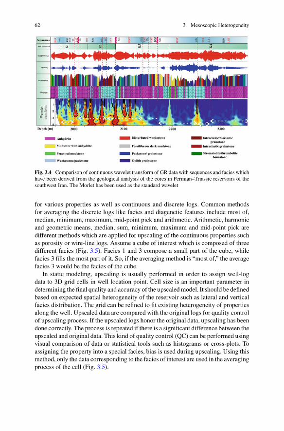
62 3 Mesoscopic Heterogeneity
Fig. 3.4 Comparison of continuous wavelet transform of GR data with sequences and facies whichhave been derived from the geological analysis of the cores in Permian–Triassic reservoirs of thesouthwest Iran. The Morlet has been used as the standard wavelet
for various properties as well as continuous and discrete logs. Common methodsfor averaging the discrete logs like facies and diagenetic features include most of,median, minimum, maximum, mid-point pick and arithmetic. Arithmetic, harmonicand geometric means, median, sum, minimum, maximum and mid-point pick aredifferent methods which are applied for upscaling of the continuous properties suchas porosity or wire-line logs. Assume a cube of interest which is composed of threedifferent facies (Fig. 3.5). Facies 1 and 3 compose a small part of the cube, whilefacies 3 fills the most part of it. So, if the averaging method is “most of,” the averagefacies 3 would be the facies of the cube.
In static modeling, upscaling is usually performed in order to assign well-logdata to 3D grid cells in well location point. Cell size is an important parameter indetermining the final quality and accuracy of the upscaledmodel. It should be definedbased on expected spatial heterogeneity of the reservoir such as lateral and verticalfacies distribution. The grid can be refined to fit existing heterogeneity of propertiesalong the well. Upscaled data are compared with the original logs for quality controlof upscaling process. If the upscaled logs honor the original data, upscaling has beendone correctly. The process is repeated if there is a significant difference between theupscaled and original data. This kind of quality control (QC) can be performed usingvisual comparison of data or statistical tools such as histograms or cross-plots. Toassigning the property into a special facies, bias is used during upscaling. Using thismethod, only the data corresponding to the facies of interest are used in the averagingprocess of the cell (Fig. 3.5).
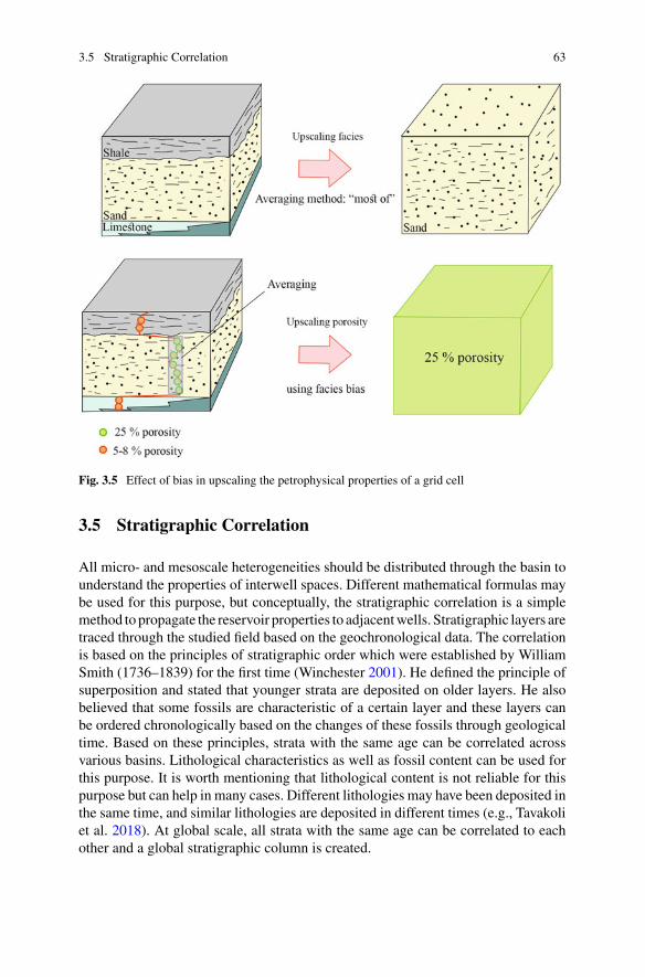
3.5 Stratigraphic Correlation 63
Fig. 3.5 Effect of bias in upscaling the petrophysical properties of a grid cell
3.5 Stratigraphic Correlation
All micro- and mesoscale heterogeneities should be distributed through the basin tounderstand the properties of interwell spaces. Different mathematical formulas maybe used for this purpose, but conceptually, the stratigraphic correlation is a simplemethod to propagate the reservoir properties to adjacentwells. Stratigraphic layers aretraced through the studied field based on the geochronological data. The correlationis based on the principles of stratigraphic order which were established by WilliamSmith (1736–1839) for the first time (Winchester 2001). He defined the principle ofsuperposition and stated that younger strata are deposited on older layers. He alsobelieved that some fossils are characteristic of a certain layer and these layers canbe ordered chronologically based on the changes of these fossils through geologicaltime. Based on these principles, strata with the same age can be correlated acrossvarious basins. Lithological characteristics as well as fossil content can be used forthis purpose. It is worth mentioning that lithological content is not reliable for thispurpose but can help in many cases. Different lithologies may have been deposited inthe same time, and similar lithologies are deposited in different times (e.g., Tavakoliet al. 2018). At global scale, all strata with the same age can be correlated to eachother and a global stratigraphic column is created.
64 3 Mesoscopic Heterogeneity
Key stratigraphic surfaces or layers are very useful in correlation of strata in abasin. A regional erosional unconformity can be correlated with high confidencethrough a field or even a basin. Volcanic ashes or the traces of meteorite in sedimentsare good examples. They represent an event in a specific time and so are correlatedover a large area.At the end of theCretaceous, a dust layer rich in iridium is detectableworldwide. Such layers or key surfaces are called chronostratigraphic markers. Thestudy of relatively short-lived stratigraphic markers is called event stratigraphy. Theterm defined by Seilacher (1991) as the sedimentarymarkers produced by sudden andusually catastrophic short time geological events. These events last for thousands ofyears or even less. Compared to those which take longer time at geological timescale,these events have been occurred in a short time at regional or global scale.
The evolutionary changes in fossils over geological times enable the correlationof the strata based on the absolute age of sediments. These changes are triggeredby abrupt and dramatic environmental variations. The extinction of a species isgeologically instantaneous and global in many cases. The planktonic fossils whichare floated on water could be correlated globally, but some others are restricted toa specific depth, environment or climate. They are used just for local correlationcompared to the first ones.
Geomagnetic polarity timescale is also used for stratigraphic correlations but islimited by the oriented sampling and magnetic minerals which should be oriented bythe earth magnetic field during deposition. The geomagnetic polarity is the result ofirregular alternations of earth’s magnetic field between two different polarity statesduring Phanerozoic. The geomagnetic polarity remains nearly constant during sometime intervals which are called polarity chrons. The present state of the polarityis called normal. So, the opposite state is reverse during the geological time. Theprofiles are compared with the standard global geometrical polarity, and the strataare correlated (e.g., Zhang et al. 2015; Bover-Arnal et al. 2016).
The seismic data are also used for stratigraphic correlations. These data are pro-vided during exploration phase of the hydrocarbon fields by seismic waves. Theformation boundaries and key stratigraphic surfaces are marked on these seismicsections and are correlated through the field or basin (see Sect. 4.1).
The strata can be correlated based on the geochemical characteristics of the car-bonate rocks. Chemostratigraphy is determining the chronological order of strata(e.g., elemental composition, stable isotope ratios), arranging them in specific andtraceable units and establishing their hierarchy and distribution, based on theirgeochemical contents (Ramkumar 2015). It is obvious from this definition thatchemostratigraphy is a useful method for stratigraphic correlations. Geochemicalsignatures of the carbonate rocks are changed based on different physical, chemicaland biological conditions of the sedimentary environments. At the large scales, theseunits are homogeneous and so their correlation can help in overcoming the chal-lenges of heterogeneity in carbonate reservoirs. The rocks are characterized basedon their geochemical signatures such as elemental concentrations or stable isotoperatios. Sharp boundaries are used for distinguishing the key surfaces. A good exam-ple is the global negative excursion of δ13C in Permian–Triassic boundary (PTB)(e.g., Dolenec et al. 2001; Heydari and Hassanzadeh 2003; Lehrmann et al. 2003;
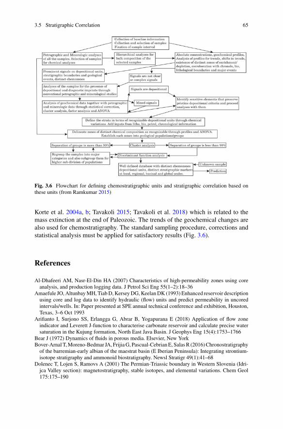
3.5 Stratigraphic Correlation 65
Fig. 3.6 Flowchart for defining chemostratigraphic units and stratigraphic correlation based onthese units (from Ramkumar 2015)
Korte et al. 2004a, b; Tavakoli 2015; Tavakoli et al. 2018) which is related to themass extinction at the end of Paleozoic. The trends of the geochemical changes arealso used for chemostratigraphy. The standard sampling procedure, corrections andstatistical analysis must be applied for satisfactory results (Fig. 3.6).
References
Al-Dhafeeri AM, Nasr-El-Din HA (2007) Characteristics of high-permeability zones using coreanalysis, and production logging data. J Petrol Sci Eng 55(1–2):18–36
Amaefule JO,AltunbayMH, TiabD,KerseyDG,KeelanDK (1993) Enhanced reservoir descriptionusing core and log data to identify hydraulic (flow) units and predict permeability in uncoredintervals/wells. In: Paper presented at SPE annual technical conference and exhibition, Houston,Texas, 3–6 Oct 1993
Arifianto I, Surjono SS, Erlangga G, Abrar B, Yogapurana E (2018) Application of flow zoneindicator and Leverett J-function to characterise carbonate reservoir and calculate precise watersaturation in the Kujung formation, North East Java Basin. J Geophys Eng 15(4):1753–1766
Bear J (1972) Dynamics of fluids in porous media. Elsevier, New YorkBover-Arnal T,Moreno-Bedmar JA, FrijiaG, Pascual-CebrianE, SalasR (2016)Chronostratigraphyof the barremian-early albian of the maestrat basin (E Iberian Peninsula): Integrating strontium-isotope stratigraphy and ammonoid biostratigraphy. Newsl Stratigr 49(1):41–68
Dolenec T, Lojen S, Ramovs A (2001) The Permian-Triassic boundary in Western Slovenia (Idri-jca Valley section): magnetostratigraphy, stable isotopes, and elemental variations. Chem Geol175:175–190

66 3 Mesoscopic Heterogeneity
Ebanks WJ (1987) The flow unit concept—an integrated approach to reservoir description forengineering projects. AAPG Meeting Abstracts 1:521–522
EllwoodBB, Tomkin JH, FeboLA, Stuart CN (2008) Time series analysis ofmagnetic susceptibilityvariations in deep marine sedimentary rocks: a test using the upper Danian-Lower Selandianproposed GSSP, Spain. Palaeogeogr Palaeocl Palaeoeco 261(3–4):270–279
Eltom H, Makkawi M, Abdullatif O, Alramadan K (2013) High-resolution facies and porositymodels of the upper Jurassic Arab-D carbonate reservoir using an outcrop analogue, centralSaudi Arabia. Arab J Geosci 6(11):4323–4335
Farshi M, Moussavi-Harami R, Mahboubi A, Khanehbad M, Golafshani T (2019) Reservoir rocktyping using integrating geological and petrophysical properties for the Asmari Formation in theGachsaran oil field, Zagros basin. J Petrol Sci Eng 176:161–171
Flugel E (2010) Microfacies of carbonate rocks, analysis, interpretation and application. Springer,Berlin
Ginsburg RN, James NP (1974) Holocene carbonate sediments of continental shelfs. The geologyof continetal margins. Springer, Berlin, pp 137–155
Gunter GW, Finneran JM, HartmanDJ,Miller JD (1997) Early determination of reservoir flow unitsusing an integrated petrophysical method, SPE 38679. In: SSPE annual technical conference andexhibition. San Antonio, TX; October 5–8, 1997
Hear CL, Ebanks WJ, Tye RS and Ranganatha V (1984) Geological Factors Influencing ReservoirPerformance of the Hartzog Draw Field, Wyoming. J Petrol Tech, 1335–1344
Herbert TD, FischerAG (1986)Milankovitch climatic origin ofmid-Cretaceous black shale rhythmsin central Italy. Nature 321:739–743
Heydari E,Hassanzadeh J (2003)Deevjahimodel of the Permian-Triassic boundarymass extinction:a case for gas hydrates as themain cause of biological crisis onEarth. SedimentGeol 163:147–163
IzadiM, Ghalambor A (2013) New approach in permeability and hydraulic-flow unit determination.SPE Reserv Eval Eng 16(3):257–264
Jennings JW,Ruppel SC,WardWB(2000)Geostatistical analysis of permeability data andmodelingof fluid-flow effects in carbonate outcrops. SPEREE 3:292–303
Jensen JL, Lake LW, Corbett PW, Goggin DJ (2000) Statistics for petroleum engineers andgeoscientists. Elsevier, Amsterdam, p 338
Korte C, Kozur HW, Joachimski MM, Strauss H, Veizer J, Schwark L (2004a) Carbon, sulfur,oxygen and strontium isotope records, organic geochemistry and biostratigraphy across thePermian/Triassic boundary in Abadeh, Iran. Int J Earth Sci 93:565–581
Korte C, Kozur HW, Mohtat-Aghai P (2004b) Dzhulfian to lowermost Triassic δ13C recordat the Permian/Triassic boundary section at Shahreza, Central Iran. Hallesches Jahrb derGeowissenschaften Beiheft 18:73–78
Lehrmann DJ, Payne JL, Felix SV, Dillett PM, Wang H, Yu Y, Wei J (2003) Permian-Triassicboundary sections from shallow-marine carbonate platforms of the Nanpanjiang Basin, SouthChina: implications for oceanic conditions associated with the end-Permian extinction and itsaftermath. Palaios 18:138–152
Lerat O, Van Buchem FSP, Eschard R, Grammer GM, Homewood PW (2000) Facies distributionand control by accommodation within high-frequency cycles of the Upper Ismay interval (Penn-sylvanian, Paradox Basin, Utah). In: Homewood PW, Eberli GP (eds) Genetic stratigraphy at theexploration and production scales. Elf EP, Pau, France, pp 71–91
Liu Z (2012) Orbital cycles analysis and its genesis significance for the sequence hierarchy: a casestudy of Carboniferous Karashayi Formation, Central Tarim basin. J Earth Sci 23(4):516–528
Liu Y, Liu Y, Zhang Q, Li C, Feng Y, Wang Y, Xue Y, Ma H (2019) Petrophysical static rock typingfor carbonate reservoirs based on mercury injection capillary pressure curves using principalcomponent analysis. J Petrol Sci Eng 181:106175
Mirzaei-Paiaman A, Saboorian-Jooybari H, Pourafshary P (2015) Improved method to identifyhydraulic flow units for reservoir characterization. Energy Technol 3:726–733
Mirzaei-Paiaman A, Ostadhassan M, Rezaee R, Saboorian-Jooybari H, Chen Z (2018) A newapproach in petrophysical rock typing. J Petr Sci Eng 166:445–464

References 67
Mirzaei-PaiamanA, Sabbagh F, OstadhassanM, Shafiei A, RezaeeMR, Saboorian-Jooybari H, CheZ (2019) A further verification of FZI and PSRTI: newly developed petrophysical rock typingindices. J Petr Sci Eng 175:693–705
Nabawy BS, Rashed MA, Mansour AS, Afify WSM (2018) Petrophysical and microfacies analysisas a tool for reservoir rock typing and modeling: Rudeis Formation, off-shore October Oil Field,Sinai. Mar Petrol Geol 97:260–276
Nazari MH, Tavakoli V, Rahimpour-Bonab H, Sharifi-Yazdi M (2019) Investigation of factorsinfluencing geological heterogeneity in tight gas carbonates, Permian reservoir of the PersianGulf. J Petrol Sci Eng 183, art. no 106341
Prokoph A, Agterberg FP (2000) Wavelet analysis of well-logging data from oil source rock, EgretMember, Offshore Eastern Canada. AAPG Bull 84(10):1617–1632
Prokoph A, Thurow J (2000) Diachronous pattern of Milankovitch cyclicity in late Albian pelagicmarlstones of the North German Basin. Sed Geol 134(3–4):287–303
Prokoph A, Shields GA, Veizer J (2008) Compilation and time-series analysis of a marine carbonateδ18O, δ13C, 87Sr/86Sr and δ34S database through earth history. Earth-Sci Rev 87(3–4):113–133
Rahimpour-Bonab H, Mehrabi H, Navidtalab A, Izadi-Mazidi E (2012) Flow unit distribution andreservoirmodelling in cretaceous carbonates of theSarvakFormation,AbteymourOilfield,DezfulEmbayment, SW Iran. J Petr Geol 35(3):213–236
Ramkumar M (2015) Chemostratigraphy: concepts, techniques and applications. Elsevier, Amster-dam
Read JF (1982) Carbonate platforms of passive (extensional) continental margins: types, character-istics and evolution. Tectonophysics 81:195–212
Riazi Z (2018) Application of integrated rock typing and flow units identification methods for anIranian carbonate reservoir. J Petr Sci Eng 160:483–497
Schwarzacher W (1993) Cyclostratigraphy and Milankovitch theory. Devel Sedimentol 52:225Seilacher A (1991) Events and their signatures: an overview. In: Einsele G, Ricken W, Seilacher A(eds) Cycles and events in stratigraphy. Springer, Berlin, Heidelberg, New York, p 955
Shaw AB (1964) Time in stratigraphy, 365. McGraw-Hill Book Company, New YorkSoleymanzadeh A, Parvin S, Kord S (2019) Effect of overburden pressure on determination ofreservoir rock types using RQI/FZI, FZI and Winland methods in carbonate rocks. Petr Sci.https://doi.org/10.1007/s12182-019-0332-8
Tavakoli V (2015) Chemostratigraphy of the Permian-Triassic Strata of the Offshore Persian Gulf,Iran. In: Ramkumar M (ed) Chemostratigraphy: concepts, techniques, and applications. Elsevier,Amsterdam
Tavakoli V (2018) Geological core analysis: application to reservoir characterization. Springer,Cham
Tavakoli V, Rahimpour-Bonab H, Esrafili-Dizaji B (2011) Diagenetic controlled reservoir qualityof South Pars gas field, an integrated approach. C R Geosci 343:55–71
Tavakoli V, Naderi-Khujin M, Seyedmehdi Z (2018) The end-Permian regression in the westernTethys: sedimentological and geochemical evidence from offshore the Persian Gulf, Iran. Geo-Mar Lett 38(2):179–192
Tiab D, Donaldson EC (2015) Petrophysics, theory and practice of measuring reservoir rock andfluid transport properties. Gulf Professional Publishing, Houston
Walker RG (1984) Facies models. Geological Association of CanadaWinchester S (2001) The map that changed the World. Harper Collins, New York, p 329Zhang Y, Li M, Ogg JG, Montgomery P, Huang C, Chen ZQ, Shi Z, Enos P, Lehrmann DJ (2015)Cycle-calibrated magnetostratigraphy of middle Carnian from South China: implications forLate Triassic time scale and termination of the Yangtze Platform. Palaeogeo Palaeocl Palaeoeco436:135–166
Chapter 4Macroscopic Heterogeneity
Abstract Microscopic andmesoscopic heterogeneities should be combined to formlarger-scale units which can be correlated across the field or basin. This is performedby using seismic data, sedimentary strata, sequence stratigraphic concepts, construct-ing variousmaps and reservoir tomography. Seismicwaves pass through the reservoirrocks and illustrate the large-scale structures. These data are very useful for detailedsubsurface correlations at field scale. Layers with acoustic impedance contrast rep-resent different zones. They should be carefully interpreted. These seismic linesmay indicate formation tops, chronological boundaries, different lithologies or anychange in reservoir properties. Stratification is caused by changes in facies prop-erties through time. They represent different depositional conditions and probablyreservoir characteristics. The widespread lateral continuity of the strata makes themuseful for large-scale correlations.Genetically related strata are classified as sequencestratigraphic units. These units are deposited in the same physical, chemical and bio-logical conditions, and so, they usually have similar reservoir properties.With respectto their primary textures, they also have the same diagenetic imprints. The bound-aries between these units are marked based on the core analysis data, seismic tracesand wire-line logs. They are correlated between the wells as reservoir zones. Then,microscopic and mesoscopic scale units are distributed in sequence stratigraphicframework. Low permeability or impermeable layers or strata are considered as staticor dynamic compartmentalizers in the reservoir body. They strongly affect the fluidproperties of reservoir compartments and so should be carefully considered beforeproduction. Data from various wells are projected on horizontal planes as maps oron vertical sections as profiles. They help to improve the macroscopic understandingof the reservoir heterogeneities. The horizontal maps of different depths are used forreservoir tomography. The variations in properties through time are revealed withthis method.
© The Author(s), under exclusive license to Springer Nature Switzerland AG 2020V. Tavakoli, Carbonate Reservoir Heterogeneity,SpringerBriefs in Petroleum Geoscience & Engineering,https://doi.org/10.1007/978-3-030-34773-4_4
69
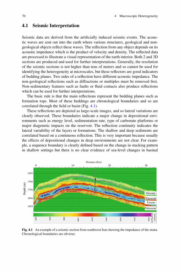
70 4 Macroscopic Heterogeneity
4.1 Seismic Interpretation
Seismic data are derived from the artificially induced seismic events. The acous-tic waves are sent out into the earth where various structures, geological and non-geological objects reflect these waves. The reflection from any object depends on itsacoustic impedance which is the product of velocity and density. The reflected dataare processed to illustrate a visual representation of the earth interior. Both 2 and 3Dsections are produced and used for further interpretations. Generally, the resolutionof the seismic sections is not higher than tens of meters and so cannot be used foridentifying the heterogeneity at microscales, but these reflectors are good indicatorsof bedding planes. Two sides of a reflection have different acoustic impedance. Thenon-geological reflections such as diffractions or multiples must be removed first.Non-sedimentary features such as faults or fluid contacts also produce reflectionswhich can be used for further interpretations.
The basic rule is that the main reflections represent the bedding planes such asformation tops. Most of these beddings are chronological boundaries and so arecorrelated through the field or basin (Fig. 4.1).
These reflections are depicted as large-scale images, and so lateral variations areclearly observed. These boundaries indicate a major change in depositional envi-ronments such as energy level, sedimentation rate, type of carbonate platforms ormajor diagenetic impacts on the reservoir. The reflection continuity indicates thelateral variability of the layers or formations. The shallow and deep sediments arecorrelated based on a continuous reflection. This is very important because usuallythe effects of depositional changes in deep environments are not clear. For exam-ple, a sequence boundary is clearly defined based on the change in stacking patternin shallow settings but there is no clear evidence of sea-level changes in basinal
Fig. 4.1 An example of a seismic section from southwest Iran showing the impedance of the strata.Chronological boundaries are obvious
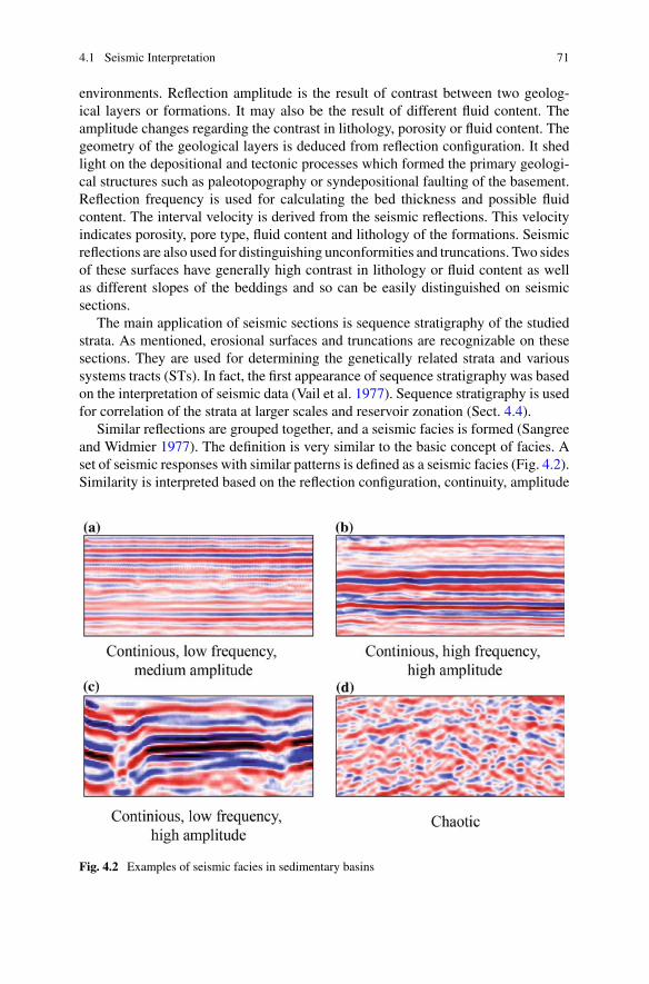
4.1 Seismic Interpretation 71
environments. Reflection amplitude is the result of contrast between two geolog-ical layers or formations. It may also be the result of different fluid content. Theamplitude changes regarding the contrast in lithology, porosity or fluid content. Thegeometry of the geological layers is deduced from reflection configuration. It shedlight on the depositional and tectonic processes which formed the primary geologi-cal structures such as paleotopography or syndepositional faulting of the basement.Reflection frequency is used for calculating the bed thickness and possible fluidcontent. The interval velocity is derived from the seismic reflections. This velocityindicates porosity, pore type, fluid content and lithology of the formations. Seismicreflections are also used for distinguishing unconformities and truncations. Two sidesof these surfaces have generally high contrast in lithology or fluid content as wellas different slopes of the beddings and so can be easily distinguished on seismicsections.
The main application of seismic sections is sequence stratigraphy of the studiedstrata. As mentioned, erosional surfaces and truncations are recognizable on thesesections. They are used for determining the genetically related strata and varioussystems tracts (STs). In fact, the first appearance of sequence stratigraphy was basedon the interpretation of seismic data (Vail et al. 1977). Sequence stratigraphy is usedfor correlation of the strata at larger scales and reservoir zonation (Sect. 4.4).
Similar reflections are grouped together, and a seismic facies is formed (Sangreeand Widmier 1977). The definition is very similar to the basic concept of facies. Aset of seismic responses with similar patterns is defined as a seismic facies (Fig. 4.2).Similarity is interpreted based on the reflection configuration, continuity, amplitude
Fig. 4.2 Examples of seismic facies in sedimentary basins
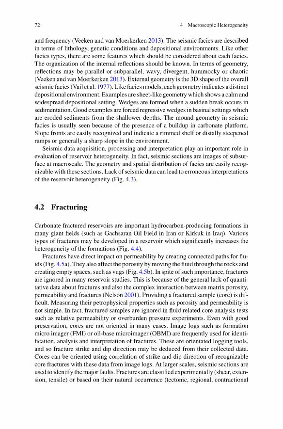
72 4 Macroscopic Heterogeneity
and frequency (Veeken and van Moerkerken 2013). The seismic facies are describedin terms of lithology, genetic conditions and depositional environments. Like otherfacies types, there are some features which should be considered about each facies.The organization of the internal reflections should be known. In terms of geometry,reflections may be parallel or subparallel, wavy, divergent, hummocky or chaotic(Veeken and vanMoerkerken 2013). External geometry is the 3D shape of the overallseismic facies (Vail et al. 1977). Like faciesmodels, each geometry indicates a distinctdepositional environment. Examples are sheet-like geometrywhich shows a calm andwidespread depositional setting. Wedges are formed when a sudden break occurs insedimentation.Good examples are forced regressivewedges in basinal settingswhichare eroded sediments from the shallower depths. The mound geometry in seismicfacies is usually seen because of the presence of a buildup in carbonate platform.Slope fronts are easily recognized and indicate a rimmed shelf or distally steepenedramps or generally a sharp slope in the environment.
Seismic data acquisition, processing and interpretation play an important role inevaluation of reservoir heterogeneity. In fact, seismic sections are images of subsur-face at macroscale. The geometry and spatial distribution of facies are easily recog-nizable with these sections. Lack of seismic data can lead to erroneous interpretationsof the reservoir heterogeneity (Fig. 4.3).
4.2 Fracturing
Carbonate fractured reservoirs are important hydrocarbon-producing formations inmany giant fields (such as Gachsaran Oil Field in Iran or Kirkuk in Iraq). Varioustypes of fractures may be developed in a reservoir which significantly increases theheterogeneity of the formations (Fig. 4.4).
Fractures have direct impact on permeability by creating connected paths for flu-ids (Fig. 4.5a). They also affect the porosity bymoving the fluid through the rocks andcreating empty spaces, such as vugs (Fig. 4.5b). In spite of such importance, fracturesare ignored in many reservoir studies. This is because of the general lack of quanti-tative data about fractures and also the complex interaction between matrix porosity,permeability and fractures (Nelson 2001). Providing a fractured sample (core) is dif-ficult. Measuring their petrophysical properties such as porosity and permeability isnot simple. In fact, fractured samples are ignored in fluid related core analysis testssuch as relative permeability or overburden pressure experiments. Even with goodpreservation, cores are not oriented in many cases. Image logs such as formationmicro imager (FMI) or oil-base microimager (OBMI) are frequently used for identi-fication, analysis and interpretation of fractures. These are orientated logging tools,and so fracture strike and dip direction may be deduced from their collected data.Cores can be oriented using correlation of strike and dip direction of recognizablecore fractures with these data from image logs. At larger scales, seismic sections areused to identify themajor faults. Fractures are classified experimentally (shear, exten-sion, tensile) or based on their natural occurrence (tectonic, regional, contractional
4.2 Fracturing 73
Fig. 4.3 Correlation of three wells in a field. Some seismic anomalies are not clear in log-basedcorrelation (a) while they are recognizable using seismic data (b, c)
and surface-related) (Nelson 2001). Contractional fractures have negligible effect onreservoir properties (Fig. 4.5c–e). To understand the effect of fractures on reservoirquality and heterogeneity, the petrophysical properties of the fractures’ networkmustbe addressed. These properties include fracture type, dimension, and morphology,stratigraphically and spatially fracture distribution, geological characteristics (suchas cementation or variations due to preferential lithology), structural evolution andpetrophysical properties resulting from fracture system of the rocks. Petrophysicalproperties include permeability and porosity of the fracture, fluid saturation and therecovery factor expected from the fractures of the reservoir (Nelson 2001). In caseof permeability, fractures considerably change the anisotropy and heterogeneity of

74 4 Macroscopic Heterogeneity
Fig. 4.4 Different types of fractures are developed in a reservoir. They have strong effect on fluidflow and heterogeneity of the carbonates (courtesy of R. Nozaem). The figure has been compiledfrom Hatcher (1994) and Davis et al. (2011)
the rocks (e.g., Hennings et al. 2012; Guerriero et al. 2013; Wang et al. 2016; Volatiliet al. 2019).
In terms of morphology, both open and mineral-filled fractures change theheterogeneity of the reservoir. While open fractures increase the permeability ofthe reservoir, mineral filled fracture acts as fluid barriers and may produce acompartmentalizer (Fig. 4.5f) layer (e.g., Massaro et al. 2018).
All fractures are secondary in origin and so may follow the other formation prop-erties. The effect of lithology and facies characteristics on fracturing has been dis-cussed bymany authors (e.g., Moore andWade 2013;Michie 2015; Dong et al. 2017;Korneva et al. 2018). These studies indicate that lithology, crystal size, texture, bedthickness and porosity type, size and volume have strong effects on fracturing. Manyresearchers believe that fracturing is more intense in dolomites compared to lime-stone (e.g., Schmoker et al. 1985; Nelson 2001; Gale et al. 2004; Korneva et al. 2018).Some studies have documented the opposite (e.g., Beliveau et al. 1993; Rustichelliet al. 2015). Flugel (2010) and Rustichelli et al. (2015) demonstrated that fine crys-talline dolostones are densely fractured compared to coarse-crystalline dolomites.Sowers (1970) and McQuillan (1973) showed that the fracture spacing increaseswith increasing the bed thickness. So, fractures follow the precursor heterogeneityof the rocks in some cases.
Fracture analysis of outcrop sections shed light on the fracture development incarbonate reservoirs (e.g., De Keijzer et al. 2007; Bisdom et al. 2017; Burberry andPeppers 2017; Massaro et al. 2018). Outcrops are available over large areas, thegeometry and thickness of the layers can be traced continuously, and fractures are
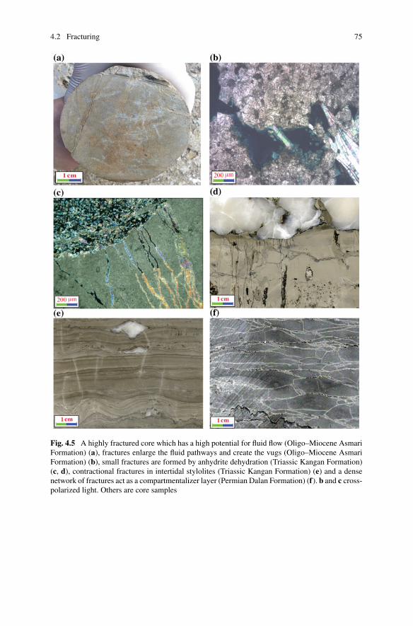
4.2 Fracturing 75
Fig. 4.5 A highly fractured core which has a high potential for fluid flow (Oligo–Miocene AsmariFormation) (a), fractures enlarge the fluid pathways and create the vugs (Oligo–Miocene AsmariFormation) (b), small fractures are formed by anhydrite dehydration (Triassic Kangan Formation)(c, d), contractional fractures in intertidal stylolites (Triassic Kangan Formation) (e) and a densenetwork of fractures act as a compartmentalizer layer (Permian Dalan Formation) (f). b and c cross-polarized light. Others are core samples
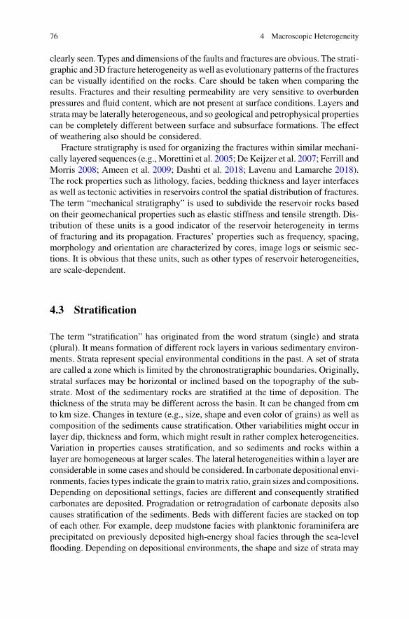
76 4 Macroscopic Heterogeneity
clearly seen. Types and dimensions of the faults and fractures are obvious. The strati-graphic and 3D fracture heterogeneity aswell as evolutionary patterns of the fracturescan be visually identified on the rocks. Care should be taken when comparing theresults. Fractures and their resulting permeability are very sensitive to overburdenpressures and fluid content, which are not present at surface conditions. Layers andstrata may be laterally heterogeneous, and so geological and petrophysical propertiescan be completely different between surface and subsurface formations. The effectof weathering also should be considered.
Fracture stratigraphy is used for organizing the fractures within similar mechani-cally layered sequences (e.g., Morettini et al. 2005; De Keijzer et al. 2007; Ferrill andMorris 2008; Ameen et al. 2009; Dashti et al. 2018; Lavenu and Lamarche 2018).The rock properties such as lithology, facies, bedding thickness and layer interfacesas well as tectonic activities in reservoirs control the spatial distribution of fractures.The term “mechanical stratigraphy” is used to subdivide the reservoir rocks basedon their geomechanical properties such as elastic stiffness and tensile strength. Dis-tribution of these units is a good indicator of the reservoir heterogeneity in termsof fracturing and its propagation. Fractures’ properties such as frequency, spacing,morphology and orientation are characterized by cores, image logs or seismic sec-tions. It is obvious that these units, such as other types of reservoir heterogeneities,are scale-dependent.
4.3 Stratification
The term “stratification” has originated from the word stratum (single) and strata(plural). It means formation of different rock layers in various sedimentary environ-ments. Strata represent special environmental conditions in the past. A set of strataare called a zone which is limited by the chronostratigraphic boundaries. Originally,stratal surfaces may be horizontal or inclined based on the topography of the sub-strate. Most of the sedimentary rocks are stratified at the time of deposition. Thethickness of the strata may be different across the basin. It can be changed from cmto km size. Changes in texture (e.g., size, shape and even color of grains) as well ascomposition of the sediments cause stratification. Other variabilities might occur inlayer dip, thickness and form, which might result in rather complex heterogeneities.Variation in properties causes stratification, and so sediments and rocks within alayer are homogeneous at larger scales. The lateral heterogeneities within a layer areconsiderable in some cases and should be considered. In carbonate depositional envi-ronments, facies types indicate the grain tomatrix ratio, grain sizes and compositions.Depending on depositional settings, facies are different and consequently stratifiedcarbonates are deposited. Progradation or retrogradation of carbonate deposits alsocauses stratification of the sediments. Beds with different facies are stacked on topof each other. For example, deep mudstone facies with planktonic foraminifera areprecipitated on previously deposited high-energy shoal facies through the sea-levelflooding. Depending on depositional environments, the shape and size of strata may
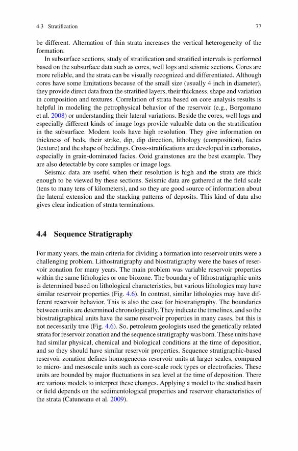
4.3 Stratification 77
be different. Alternation of thin strata increases the vertical heterogeneity of theformation.
In subsurface sections, study of stratification and stratified intervals is performedbased on the subsurface data such as cores, well logs and seismic sections. Cores aremore reliable, and the strata can be visually recognized and differentiated. Althoughcores have some limitations because of the small size (usually 4 inch in diameter),they provide direct data from the stratified layers, their thickness, shape and variationin composition and textures. Correlation of strata based on core analysis results ishelpful in modeling the petrophysical behavior of the reservoir (e.g., Borgomanoet al. 2008) or understanding their lateral variations. Beside the cores, well logs andespecially different kinds of image logs provide valuable data on the stratificationin the subsurface. Modern tools have high resolution. They give information onthickness of beds, their strike, dip, dip direction, lithology (composition), facies(texture) and the shape of beddings. Cross-stratifications are developed in carbonates,especially in grain-dominated facies. Ooid grainstones are the best example. Theyare also detectable by core samples or image logs.
Seismic data are useful when their resolution is high and the strata are thickenough to be viewed by these sections. Seismic data are gathered at the field scale(tens to many tens of kilometers), and so they are good source of information aboutthe lateral extension and the stacking patterns of deposits. This kind of data alsogives clear indication of strata terminations.
4.4 Sequence Stratigraphy
For many years, the main criteria for dividing a formation into reservoir units were achallenging problem. Lithostratigraphy and biostratigraphy were the bases of reser-voir zonation for many years. The main problem was variable reservoir propertieswithin the same lithologies or one biozone. The boundary of lithostratigraphic unitsis determined based on lithological characteristics, but various lithologies may havesimilar reservoir properties (Fig. 4.6). In contrast, similar lithologies may have dif-ferent reservoir behavior. This is also the case for biostratigraphy. The boundariesbetween units are determined chronologically. They indicate the timelines, and so thebiostratigraphical units have the same reservoir properties in many cases, but this isnot necessarily true (Fig. 4.6). So, petroleum geologists used the genetically relatedstrata for reservoir zonation and the sequence stratigraphywas born. These units havehad similar physical, chemical and biological conditions at the time of deposition,and so they should have similar reservoir properties. Sequence stratigraphic-basedreservoir zonation defines homogeneous reservoir units at larger scales, comparedto micro- and mesoscale units such as core-scale rock types or electrofacies. Theseunits are bounded by major fluctuations in sea level at the time of deposition. Thereare various models to interpret these changes. Applying a model to the studied basinor field depends on the sedimentological properties and reservoir characteristics ofthe strata (Catuneanu et al. 2009).
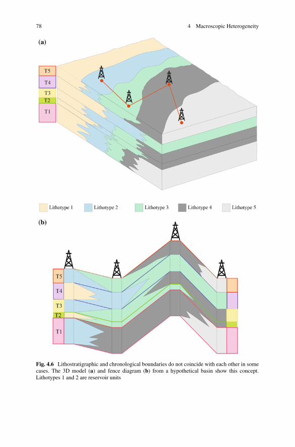
78 4 Macroscopic Heterogeneity
Fig. 4.6 Lithostratigraphic and chronological boundaries do not coincide with each other in somecases. The 3D model (a) and fence diagram (b) from a hypothetical basin show this concept.Lithotypes 1 and 2 are reservoir units
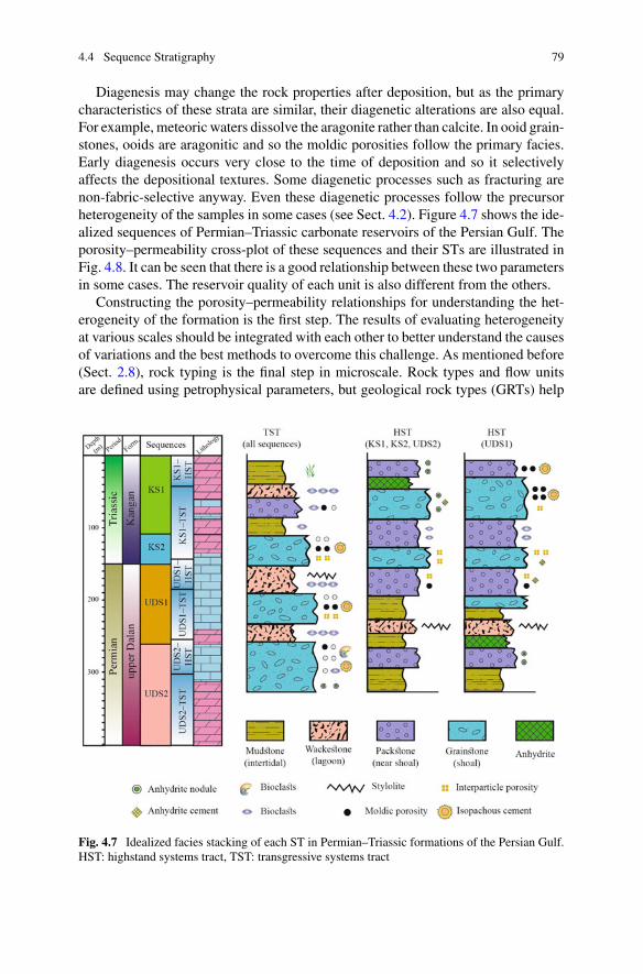
4.4 Sequence Stratigraphy 79
Diagenesis may change the rock properties after deposition, but as the primarycharacteristics of these strata are similar, their diagenetic alterations are also equal.For example, meteoric waters dissolve the aragonite rather than calcite. In ooid grain-stones, ooids are aragonitic and so the moldic porosities follow the primary facies.Early diagenesis occurs very close to the time of deposition and so it selectivelyaffects the depositional textures. Some diagenetic processes such as fracturing arenon-fabric-selective anyway. Even these diagenetic processes follow the precursorheterogeneity of the samples in some cases (see Sect. 4.2). Figure 4.7 shows the ide-alized sequences of Permian–Triassic carbonate reservoirs of the Persian Gulf. Theporosity–permeability cross-plot of these sequences and their STs are illustrated inFig. 4.8. It can be seen that there is a good relationship between these two parametersin some cases. The reservoir quality of each unit is also different from the others.
Constructing the porosity–permeability relationships for understanding the het-erogeneity of the formation is the first step. The results of evaluating heterogeneityat various scales should be integrated with each other to better understand the causesof variations and the best methods to overcome this challenge. As mentioned before(Sect. 2.8), rock typing is the final step in microscale. Rock types and flow unitsare defined using petrophysical parameters, but geological rock types (GRTs) help
Fig. 4.7 Idealized facies stacking of each ST in Permian–Triassic formations of the Persian Gulf.HST: highstand systems tract, TST: transgressive systems tract
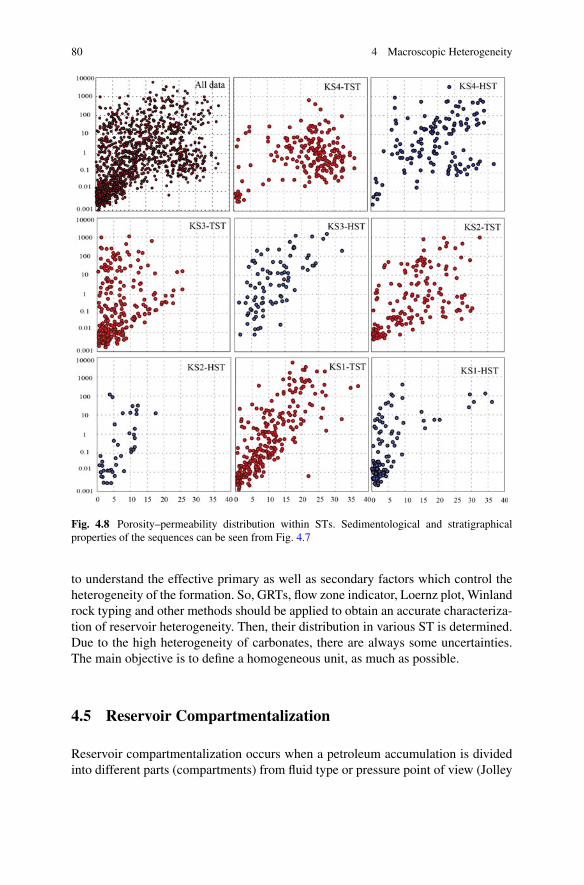
80 4 Macroscopic Heterogeneity
Fig. 4.8 Porosity–permeability distribution within STs. Sedimentological and stratigraphicalproperties of the sequences can be seen from Fig. 4.7
to understand the effective primary as well as secondary factors which control theheterogeneity of the formation. So, GRTs, flow zone indicator, Loernz plot, Winlandrock typing and other methods should be applied to obtain an accurate characteriza-tion of reservoir heterogeneity. Then, their distribution in various ST is determined.Due to the high heterogeneity of carbonates, there are always some uncertainties.The main objective is to define a homogeneous unit, as much as possible.
4.5 Reservoir Compartmentalization
Reservoir compartmentalization occurs when a petroleum accumulation is dividedinto different parts (compartments) from fluid type or pressure point of view (Jolley
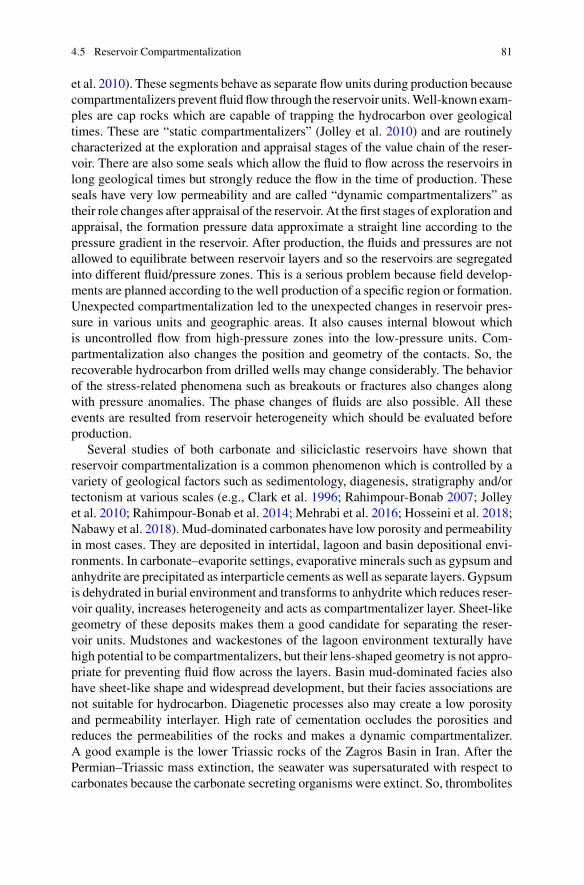
4.5 Reservoir Compartmentalization 81
et al. 2010). These segments behave as separate flow units during production becausecompartmentalizers prevent fluid flow through the reservoir units.Well-known exam-ples are cap rocks which are capable of trapping the hydrocarbon over geologicaltimes. These are “static compartmentalizers” (Jolley et al. 2010) and are routinelycharacterized at the exploration and appraisal stages of the value chain of the reser-voir. There are also some seals which allow the fluid to flow across the reservoirs inlong geological times but strongly reduce the flow in the time of production. Theseseals have very low permeability and are called “dynamic compartmentalizers” astheir role changes after appraisal of the reservoir. At the first stages of exploration andappraisal, the formation pressure data approximate a straight line according to thepressure gradient in the reservoir. After production, the fluids and pressures are notallowed to equilibrate between reservoir layers and so the reservoirs are segregatedinto different fluid/pressure zones. This is a serious problem because field develop-ments are planned according to the well production of a specific region or formation.Unexpected compartmentalization led to the unexpected changes in reservoir pres-sure in various units and geographic areas. It also causes internal blowout whichis uncontrolled flow from high-pressure zones into the low-pressure units. Com-partmentalization also changes the position and geometry of the contacts. So, therecoverable hydrocarbon from drilled wells may change considerably. The behaviorof the stress-related phenomena such as breakouts or fractures also changes alongwith pressure anomalies. The phase changes of fluids are also possible. All theseevents are resulted from reservoir heterogeneity which should be evaluated beforeproduction.
Several studies of both carbonate and siliciclastic reservoirs have shown thatreservoir compartmentalization is a common phenomenon which is controlled by avariety of geological factors such as sedimentology, diagenesis, stratigraphy and/ortectonism at various scales (e.g., Clark et al. 1996; Rahimpour-Bonab 2007; Jolleyet al. 2010; Rahimpour-Bonab et al. 2014; Mehrabi et al. 2016; Hosseini et al. 2018;Nabawy et al. 2018). Mud-dominated carbonates have low porosity and permeabilityin most cases. They are deposited in intertidal, lagoon and basin depositional envi-ronments. In carbonate–evaporite settings, evaporative minerals such as gypsum andanhydrite are precipitated as interparticle cements as well as separate layers. Gypsumis dehydrated in burial environment and transforms to anhydrite which reduces reser-voir quality, increases heterogeneity and acts as compartmentalizer layer. Sheet-likegeometry of these deposits makes them a good candidate for separating the reser-voir units. Mudstones and wackestones of the lagoon environment texturally havehigh potential to be compartmentalizers, but their lens-shaped geometry is not appro-priate for preventing fluid flow across the layers. Basin mud-dominated facies alsohave sheet-like shape and widespread development, but their facies associations arenot suitable for hydrocarbon. Diagenetic processes also may create a low porosityand permeability interlayer. High rate of cementation occludes the porosities andreduces the permeabilities of the rocks and makes a dynamic compartmentalizer.A good example is the lower Triassic rocks of the Zagros Basin in Iran. After thePermian–Triassic mass extinction, the seawater was supersaturated with respect tocarbonates because the carbonate secreting organisms were extinct. So, thrombolites
82 4 Macroscopic Heterogeneity
were expanded in the early Triassic epiric sea of the Arabian Plate. Thrombolites aremade from fine micrite particles with low permeability (Abdolmaleki and Tavakoli2016; Abdolmaleki et al. 2016). High rate of cementation also occluded the rare porespaces, and so a dynamic compartmentalizer was created (Fig. 4.9). This layer withvery low permeability allowed the hydrocarbon to flow across the Permian–Triassicboundary but acted as a seal at the time of production. So, the strata which seemedto be one reservoir, segregated into two reservoirs with different pressure regime.
Vertical sealed faults and fracturesmay compartmentalize the different geographicregions of a field (e.g., Bailey et al. 2002; Ainsworth 2006; Massaro et al. 2018). So,the field may be both horizontally and vertically compartmentalized. The fracturesor faults must be impermeable to segregate the reservoir into different regions. Thisis very important in shared fields where production from one side in one country
Fig. 4.9 Post-extinction thrombolite facies of the lower Triassic strata of Zagros Basin in thinsection (a) and SEM (b) images. Large calcite crystals have been precipitated from supersaturatedseawater (c). Energy-dispersive X-ray (EDX) analysis confirms the calcite mineralogy (d)
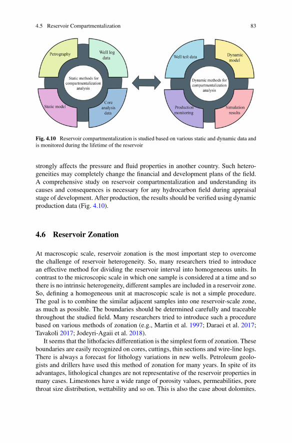
4.5 Reservoir Compartmentalization 83
Fig. 4.10 Reservoir compartmentalization is studied based on various static and dynamic data andis monitored during the lifetime of the reservoir
strongly affects the pressure and fluid properties in another country. Such hetero-geneities may completely change the financial and development plans of the field.A comprehensive study on reservoir compartmentalization and understanding itscauses and consequences is necessary for any hydrocarbon field during appraisalstage of development. After production, the results should be verified using dynamicproduction data (Fig. 4.10).
4.6 Reservoir Zonation
At macroscopic scale, reservoir zonation is the most important step to overcomethe challenge of reservoir heterogeneity. So, many researchers tried to introducean effective method for dividing the reservoir interval into homogeneous units. Incontrast to the microscopic scale in which one sample is considered at a time and sothere is no intrinsic heterogeneity, different samples are included in a reservoir zone.So, defining a homogeneous unit at macroscopic scale is not a simple procedure.The goal is to combine the similar adjacent samples into one reservoir-scale zone,as much as possible. The boundaries should be determined carefully and traceablethroughout the studied field. Many researchers tried to introduce such a procedurebased on various methods of zonation (e.g., Martin et al. 1997; Daraei et al. 2017;Tavakoli 2017; Jodeyri-Agaii et al. 2018).
It seems that the lithofacies differentiation is the simplest form of zonation. Theseboundaries are easily recognized on cores, cuttings, thin sections and wire-line logs.There is always a forecast for lithology variations in new wells. Petroleum geolo-gists and drillers have used this method of zonation for many years. In spite of itsadvantages, lithological changes are not representative of the reservoir properties inmany cases. Limestones have a wide range of porosity values, permeabilities, porethroat size distribution, wettability and so on. This is also the case about dolomites.

84 4 Macroscopic Heterogeneity
So, the application of lithological zonation is limited to new drilled wells, especiallyin less known fields. Fossil contents are also used for zonation of the carbonatereservoirs. Chronological boundaries are determined using paleontological studies.These boundaries usually coincidewith reservoir zones because age-related strata aredeposited in similar conditions. Unconformities are good examples of time surfacesin reservoirs (e.g., Tavakoli et al. 2018). They control the reservoir characteristicsof their lower and upper strata (e.g., Abdolmaleki et al. 2016). This criterion is notapplicable when index fossils are not present. Also, change in reservoir properties isnot related to time in some cases. Instead, lateral changes in depositional environ-ments strongly affect the reservoir potential of the rocks. These environments withdifferent reservoir properties are deposited simultaneously. Instead, sequence strati-graphic surfaces are defined based on the genetic relationships between strata. Thesesediments have been deposited in similar physical, geochemical and biological con-ditions which cause their same reservoir properties. As mentioned earlier, diageneticprocesses, especially early diagenesis, are usually similar in these sedimentary rocks.So, the accepted method for reservoir zonation is sequence stratigraphy. The mostimportant aspect is that many sequence stratigraphic concepts are model-dependent(Catuneanu et al. 2009; Catuneanu 2019) and so an appropriate model should beselected to fulfill the changes in reservoir properties. Anyway, model-independentsequence stratigraphic aspects are used as the standard criteria in various geologicalsettings, scales and for different available data. At first, stratal stacking patterns arerecognized and the framework of STs is defined. These are model-independent andso can be defined in any basin or field. Then, sequence boundaries are selected andspecific types of STs are delineated. The last two, however, are model-dependent andshould be selected according to the conditions of the case study such as availabletype and resolution of data, depositional environments, tectonics and paleoclimate.For example, the forced regressive systems tract (FRST) is not recognizable in aridcarbonate ramps inmany cases. Definedmicroscale rock types and flowunits are thendistributed in STs and the degree of heterogeneity is determined. This can be startedfrom a simple porosity–permeability cross-plot in one zone (ST or sequence) andcontinuewith distributing geological rock types (GRTs) in these units. The frequencyof core-scale rock types in each sequence stratigraphic unit is also considered whichindicate the degree of heterogeneity in a zone. Other statistical parameters such ascoefficient of variation or suitable charts such as pie diagrams or histograms areapplied in order to evaluate the heterogeneity of each unit. It is obvious that anydefined zone must be traceable, mappable and correlatable through the field or eventhe basin. This, in turn, can achieve using the wire-line log data. Defined boundariesare correlated with the peaks or trough of the various logs. Wire-log log characteris-tics of each zone are extracted and correlated across the field or basin. Electrofacies(EF) (Sect. 2.9) are also used for such correlations. Like rock types, distribution ofEFs is also considered in each zone and they are traced in other wells with no cores.
Vertical distribution of flowunits can also indicate the reservoir zones. Cumulativeplot of flow units versus depth shows the reservoir boundaries. In a perfect equalitysituation when there is no vertical heterogeneity in the reservoir, the increasing ratewith depth is constant. So, plotting depth versus cumulative flow zones gives a
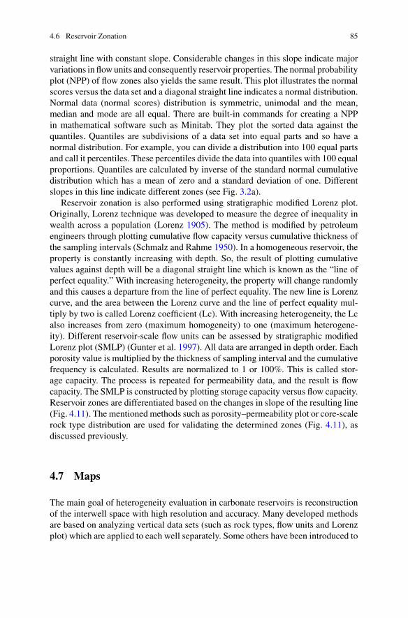
4.6 Reservoir Zonation 85
straight line with constant slope. Considerable changes in this slope indicate majorvariations in flowunits and consequently reservoir properties. The normal probabilityplot (NPP) of flow zones also yields the same result. This plot illustrates the normalscores versus the data set and a diagonal straight line indicates a normal distribution.Normal data (normal scores) distribution is symmetric, unimodal and the mean,median and mode are all equal. There are built-in commands for creating a NPPin mathematical software such as Minitab. They plot the sorted data against thequantiles. Quantiles are subdivisions of a data set into equal parts and so have anormal distribution. For example, you can divide a distribution into 100 equal partsand call it percentiles. These percentiles divide the data into quantiles with 100 equalproportions. Quantiles are calculated by inverse of the standard normal cumulativedistribution which has a mean of zero and a standard deviation of one. Differentslopes in this line indicate different zones (see Fig. 3.2a).
Reservoir zonation is also performed using stratigraphic modified Lorenz plot.Originally, Lorenz technique was developed to measure the degree of inequality inwealth across a population (Lorenz 1905). The method is modified by petroleumengineers through plotting cumulative flow capacity versus cumulative thickness ofthe sampling intervals (Schmalz and Rahme 1950). In a homogeneous reservoir, theproperty is constantly increasing with depth. So, the result of plotting cumulativevalues against depth will be a diagonal straight line which is known as the “line ofperfect equality.” With increasing heterogeneity, the property will change randomlyand this causes a departure from the line of perfect equality. The new line is Lorenzcurve, and the area between the Lorenz curve and the line of perfect equality mul-tiply by two is called Lorenz coefficient (Lc). With increasing heterogeneity, the Lcalso increases from zero (maximum homogeneity) to one (maximum heterogene-ity). Different reservoir-scale flow units can be assessed by stratigraphic modifiedLorenz plot (SMLP) (Gunter et al. 1997). All data are arranged in depth order. Eachporosity value is multiplied by the thickness of sampling interval and the cumulativefrequency is calculated. Results are normalized to 1 or 100%. This is called stor-age capacity. The process is repeated for permeability data, and the result is flowcapacity. The SMLP is constructed by plotting storage capacity versus flow capacity.Reservoir zones are differentiated based on the changes in slope of the resulting line(Fig. 4.11). The mentioned methods such as porosity–permeability plot or core-scalerock type distribution are used for validating the determined zones (Fig. 4.11), asdiscussed previously.
4.7 Maps
The main goal of heterogeneity evaluation in carbonate reservoirs is reconstructionof the interwell space with high resolution and accuracy. Many developed methodsare based on analyzing vertical data sets (such as rock types, flow units and Lorenzplot) which are applied to each well separately. Some others have been introduced to
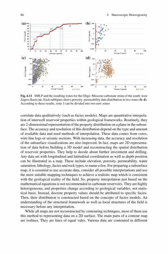
86 4 Macroscopic Heterogeneity
Fig. 4.11 SMLP and the resulting zones for the Oligo–Miocene carbonate strata of the south–westZagros Basin (a). Each subfigure shows porosity–permeability data distribution in two zones (b–d).According to these results, zone 3 can be divided into two new zones
correlate data qualitatively (such as facies models). Maps are quantitative interpola-tion of interwell reservoir properties within geological frameworks. Routinely, theyare 2-dimensional representation of the property distribution on a plane in the subsur-face. The accuracy and resolution of this distribution depend on the type and amountof available data and used methods of interpolation. These data comes from cores,wire-line logs or seismic sections. With increasing data, the accuracy and resolutionof the subsurface visualizations are also improved. In fact, maps are 2D representa-tion of data before building a 3D model and reconstructing the spatial distributionof reservoir properties. They help to decide about further investment and drilling.Any data set with longitudinal and latitudinal coordination as well as depth positioncan be illustrated as a map. These include elevation, porosity, permeability, watersaturation, lithology, facies and rock types, to name a few. For preparing a subsurfacemap, it is essential to use accurate data, consider all possible interpretations and usethe most suitable mapping techniques to achieve a realistic map which is consistentwith the geological reality of the field. So, property interpolation just based on themathematical equations is not recommended in carbonate reservoirs. They are highlyheterogeneous, and properties change according to geological variables, not statis-tical basis. Instead, discrete property values should be attributed to specific facies.Then, their distribution is constructed based on the concepts of facies models. Anunderstanding of the structural framework as well as local structures of the field isnecessary before any interpretation.
While all maps are not reconstructed by contouring techniques, most of them usethis method to representing data on a 2D surface. The main parts of a contour mapare isolines. They are lines of equal vales. Various data are contoured in different

4.7 Maps 87
maps. For example, points with the same stratigraphic thickness can be connected toeach other and an isopach map is constructed. A proper contour interval is selectedbased on the range of data. There are some basic rules that must be followed duringcontouring. For example, contours cannot cross each other. This is obvious becausea point has just one value. Closer contours indicate higher gradient and vice versa.Routinely, data are contoured by computers because they are very fast and accurate.The user chooses a proper contouring algorithm to achieve a realistic map. Ideally, agridwith regularly spacedX,Y andZ ismade.Then, the grid nods (grid line intersects)are calculated based on the available data and the final contour map is constructedbased on this grid. The spacing and so the number of nodes are determined by userbased on the real data spacing.
Various types of subsurface maps are utilized to understand the heterogeneity ofcarbonate reservoirs. The most commonly used is structural contour map. This mapmarks a key horizon or surface in terms of its elevation regarding a horizontal datumwhich is usually mean sea level. The points are routinely obtained by drilling. Thestructural contour map of formation top is useful for future drilling programs andalso understanding the reservoir geometry. An isopach map shows the true strati-graphic thickness of an individual unit. The contours are called isopach lines whichindicate the same thickness of the unit of interest. Widely spaced lines mean slightlateral thickness variations and closely spaced lines represent rapid changes in thick-ness. These types of maps are utilized to understand the geometry and volume of thereservoir rocks, recognizing the stratigraphic traps, identifying depositional environ-ments and positioning new wells for exploration and production. An isochore mapillustrates the vertical thickness of a unit, layer or formation.
Facies maps show the variations in facies. They are very useful to evaluate the het-erogeneity and understanding the distribution of properties in the reservoir becauseparticular facies commonly have their unique reservoir characteristics. The lateralextent and variations in reservoir and non-reservoir zones can be identified with thesemaps. A facies map can be generated just based on gross lithologies, but for moresophisticated exploration purposes, it is necessary to create a detailed facies map toaccurately locate the hydrocarbon-bearing intervals. Various types of facies mapsinclude:
• Lithology maps which illustrate the lithology distribution.• Isolith maps show the thickness of single lithology.• Percentage map which the contours indicate the percentage of a single unit in adesired thickness.
• Ratio maps that are generated based on the ratio of two lithologies. The mud-dominated/grain-dominated ratio is a good example in carbonate reservoirs.
• Triangle facies maps are used for depicting the ratio of three lithologies. Actually,these are not contourmaps. The ratios of various lithologies or facies are illustratedusing the patterns and shadings. Each lithology or facies type lies at one apex ofa triangle, and their ratios are characterized by different patterns (Fig. 4.12). Eachdata point in the reservoir has a known ratio of three facies. These values areconnected to each other, and the final map is constructed (Fig. 4.12).

88 4 Macroscopic Heterogeneity
Fig. 4.12 A triangle map of a Jurassic carbonate formation in northwest Iran
A paleogeographic map represents the geographic position of the geological char-acteristics in the past. Some types of these maps are useful for understanding thereservoir heterogeneity. For example, they may represent the distribution of variousfacies or lithologies in different geographic positions in a specific geological time.This helps to understand the type of sedimentary environments and reservoir rocks’distribution. In these maps, the topmost deposits are removed and the geological mapof the area at the time of deposition is illustrated.
In a reservoir with no major structural and tectonic elements, drawing the mapsfollows the basic rules of contouring but main faults can change the rules. Themain problem is that detecting subsurface faults is difficult. They are not adequatelyrevealed by contouring. Normal faults result in missing stratigraphic intervals in thewells, while reverse faults repeat the intervals. Both missing and repeated sectionsmay be revealed by comparing wire-line logs from at least two wells (Fig. 4.13).
Major faults are also detectable on seismic sections. Surface mapping and fieldobservations are helpful in some cases.
Sections and profiles are 2D correlations of wells. The interwell space is projectedonto a vertical plane, and so the properties can be traced along a specific direction(Fig. 4.14). Fence diagrams are 2D sections which are viewed in a 3D space. Theyare very useful for comparing the distribution of the properties in various directions(Fig. 4.14).
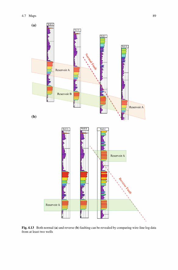
4.7 Maps 89
Fig. 4.13 Both normal (a) and reverse (b) faulting can be revealed by comparing wire-line log datafrom at least two wells
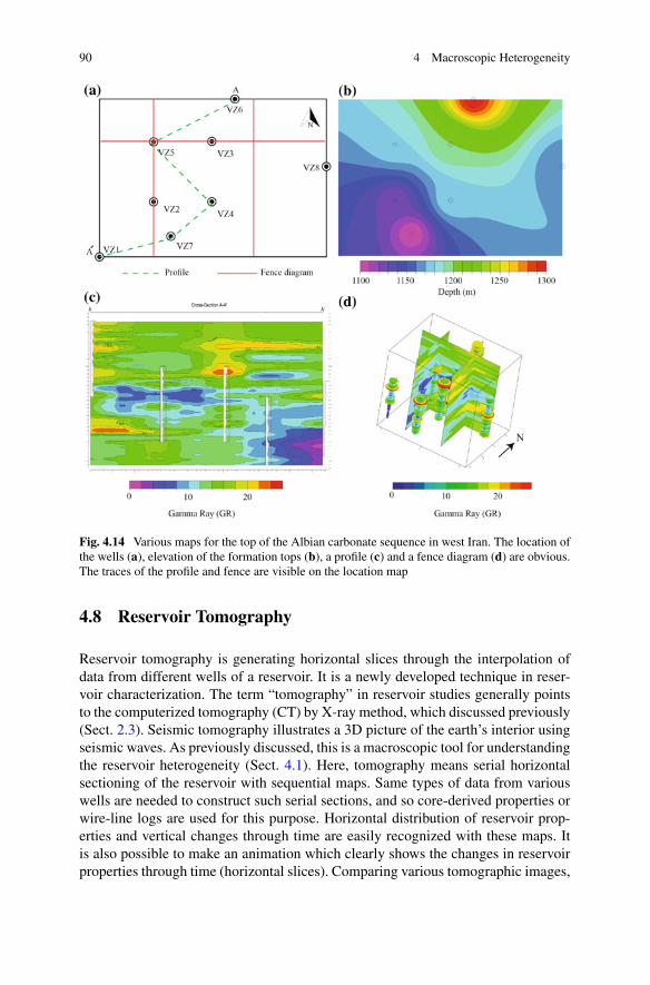
90 4 Macroscopic Heterogeneity
Fig. 4.14 Various maps for the top of the Albian carbonate sequence in west Iran. The location ofthe wells (a), elevation of the formation tops (b), a profile (c) and a fence diagram (d) are obvious.The traces of the profile and fence are visible on the location map
4.8 Reservoir Tomography
Reservoir tomography is generating horizontal slices through the interpolation ofdata from different wells of a reservoir. It is a newly developed technique in reser-voir characterization. The term “tomography” in reservoir studies generally pointsto the computerized tomography (CT) by X-ray method, which discussed previously(Sect. 2.3). Seismic tomography illustrates a 3D picture of the earth’s interior usingseismic waves. As previously discussed, this is a macroscopic tool for understandingthe reservoir heterogeneity (Sect. 4.1). Here, tomography means serial horizontalsectioning of the reservoir with sequential maps. Same types of data from variouswells are needed to construct such serial sections, and so core-derived properties orwire-line logs are used for this purpose. Horizontal distribution of reservoir prop-erties and vertical changes through time are easily recognized with these maps. Itis also possible to make an animation which clearly shows the changes in reservoirproperties through time (horizontal slices). Comparing various tomographic images,
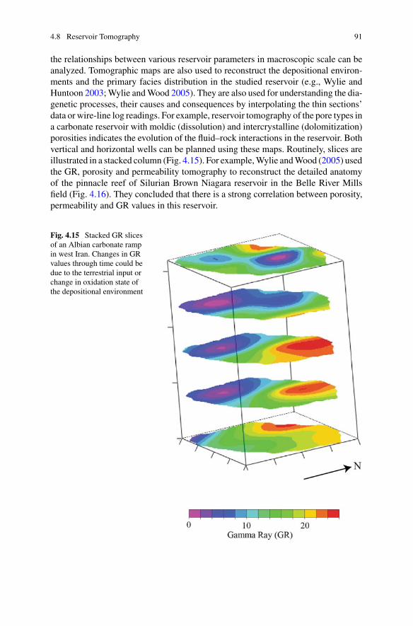
4.8 Reservoir Tomography 91
the relationships between various reservoir parameters in macroscopic scale can beanalyzed. Tomographic maps are also used to reconstruct the depositional environ-ments and the primary facies distribution in the studied reservoir (e.g., Wylie andHuntoon 2003;Wylie andWood 2005). They are also used for understanding the dia-genetic processes, their causes and consequences by interpolating the thin sections’data or wire-line log readings. For example, reservoir tomography of the pore types ina carbonate reservoir with moldic (dissolution) and intercrystalline (dolomitization)porosities indicates the evolution of the fluid–rock interactions in the reservoir. Bothvertical and horizontal wells can be planned using these maps. Routinely, slices areillustrated in a stacked column (Fig. 4.15). For example,Wylie andWood (2005) usedthe GR, porosity and permeability tomography to reconstruct the detailed anatomyof the pinnacle reef of Silurian Brown Niagara reservoir in the Belle River Millsfield (Fig. 4.16). They concluded that there is a strong correlation between porosity,permeability and GR values in this reservoir.
Fig. 4.15 Stacked GR slicesof an Albian carbonate rampin west Iran. Changes in GRvalues through time could bedue to the terrestrial input orchange in oxidation state ofthe depositional environment
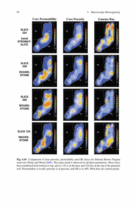
92 4 Macroscopic Heterogeneity
Fig. 4.16 Comparison of four porosity, permeability and GR slices for Silurian Brown Niagarareservoir (Wylie and Wood 2005). The same trend is observed in all three parameters. Slices havebeen numbered from bottom to top, and so 125 is at the base and 324 lies at the top of the pinnaclereef. Permeability is in mD, porosity is in percent, and GR is in API. Whit dots are control points
4.9 Macroscopic Uncertainties 93
4.9 Macroscopic Uncertainties
Uncertainty inmacroscopic heterogeneity is strongly affected by uncertainties in datagathering. The low resolution of seismic data compared with core plugs or wire-linelogs does not allow for continuous records of properties. The experience of the analystand his/her geological knowledge about the studied area have strong effect on the finalinterpretations. The situation is more complicated for fractures. Many difficultiesexist in their data acquisition, petrophysical evaluation and characterization. Theproblem is direct sampling from the reservoirs which is difficult for fracture study.Their petrophysical properties are difficult to determine because most part of thefluids flow through the fractures in laboratory tests. Quantitative approaches forfracture analysis in subsurface studies have not been developed. A deterministicapproach is necessary for understanding the fluid flow in a fractured media which isnot available yet (Nelson 2001). Image logs and seismic data can help to overcomethese difficulties, but image logs are not available from all boreholes and seismicdata have low resolution for fracture imaging.
There are also some uncertainties in sequence stratigraphy and reservoir zonation.Various models are used for determining sequences and STs in a carbonate reservoir.Selecting an appropriate model and positioning the boundaries depend on the geol-ogist’s experience. There are different criteria to distinguish a proper zone to justifythe fluid storage and flow. In many cases, the reliability of the work is determinedby distribution of microscopic results such as rock types within each zone. Thesemicroscopic units, in turn, have some uncertainties which make the problem morecomplicated. Tracing the zones and mapping their distribution is another problem.This could be unrealistic without accurate seismic data or a comprehensive geo-logical background of the field. The accuracy of a map also depends on the usedalgorithmwhich may change the result. Anyway, with all of these uncertainties, con-siderable care must be taken when predicting the spatial distribution of properties ina carbonate reservoir.
References
Abdolmaleki J, Tavakoli V (2016) Anachronistic facies in the early Triassic successions of thePersian Gulf and its palaeoenvironmental reconstruction. Palaeogeo Palaeoclimat Palaeoeco446:213–224
Abdolmaleki J, Tavakoli V, Asadi-Eskandar A (2016) Sedimentological and diagenetic controls onreservoir properties in the Permian-Triassic successions of Western Persian Gulf, Southern Iran.J Petr Sci Eng 141:90–113
Ainsworth RB (2006) Sequence stratigraphic–based analysis of reservoir connectivity: influence ofsealing faults—a case study from amarginal marine depositional setting. Petr Geosci 12:127–141
AmeenMS,SmartBGD,Somerville JMc,HammiltonS,NajiNA(2009)Predicting rockmechanicalproperties of carbonates from wireline logs (A case study: Arab–D reservoir, Ghawar field, SaudiArabia). Mar Petr Geol 26(4):430–444
94 4 Macroscopic Heterogeneity
BaileyWR,Manzocchi T et al (2002) The effect of faults on the 3D connectivity of reservoir bodies:a case study from the East Pennine Coalfield, UK. Petr Geosci 8:263–277
Beliveau D, Payne DA, Mundry M (1993) Waterflood and CO2 flood of the fractured midale field.J Petr Technol 45(9):817–881
BisdomK, Nick HM, Bertotti G (2017) An integrated workflow for stress and flowmodelling usingoutcrop–derived discrete fracture networks. Comput Geosci 103:21–35
Borgomano JRF, Fournier F, Viseur S, Rijkels L (2008) Stratigraphic well correlations for 3–Dstatic modeling of carbonate reservoirs. AAPG Bull 92(6):789–824
Burberry CM, Peppers MH (2017) Fracture characterization in tight carbonates: an example fromthe Ozark Plateau, Arkansas. AAPG Bull 101(10):1675–1696
Catuneanu O (2019) Model–independent sequence stratigraphy. Earth-Sci Rev 188:312–388Catuneanu O, Abreu V, Bhattacharya JP, Blum MD, Dalrymple RW, Eriksson PG, Fielding CR,Fisher WL, Galloway WE, Gibling MR, Giles KA, Holbrook JM, Jordan R, Kendall CGStC,Macurda B, Martinsen OJ, Miall AD, Neal JE, Nummedal D, Pomar L, Posamentier HW, PrattBR, Sarg JF, Shanley KW, Steel RJ, Strasser A, Tucker ME, Winker C (2009) Towards thestandardization of sequence stratigraphy. Earth–Sci Rev 92(1–2):1–33
Clark MS, Beckley LM, Crebs TJ, Singleton MT (1996) Tectono–eustatic controls on reservoircompartmentalisation and quality—an example from the upper miocene of the San Joaquin basin,California. Mar Petr Geol 13(5):475–491
DaraeiM,Bayet-Goll A,AnsariM (2017)An integrated reservoir zonation in sequence stratigraphicframework: A case from the Dezful Embayment, Zagros, Iran. J Petr Sci Eng 154:389–404
Dashti R, Rahimpour-Bonab H, Zeinali M (2018) Fracture and mechanical stratigraphy in naturallyfractured carbonate reservoirs–a case study from Zagros region. Mar Petr Geol 97:466–479
Davis GH, Reynolds SJ, Kluth CF (2011) Structural geology of rocks and regions. Wiley, Hoboken,NJ
De Keijzer M, Hillgartner H, Al Dhahab S, Rawnsley K (2007) A surface–subsurface study ofreservoir–scale fracture heterogeneities in Cretaceous carbonates. N Om Geol Soc Spec Publ270:227–244
Dong T, Harris NB, Ayranci K, Yang S (2017) The impact of rock composition on geomechanicalproperties of a shale formation: middle and Upper Devonian Horn River Group shale, NortheastBritish Columbia, Canada. AAPG Bull 101(2):177–204
Ferrill DA, Morris AP (2008) Fault zone deformation controlled by carbonate mechanicalstratigraphy, Balcones fault system, Texas. AAPG Bull 92(3):359–380
Flugel E (2010) Microfacies of carbonate rocks. Analysis, interpretation and application, 2nd ed, p984 XXIII
Gale JFW, Laubach SE, Marrett RA, Olson JE, Holder J, Reed RM (2004) Predicting and charac-terizing fractures in dolostone reservoirs: using the link between diagenesis and fracturing. In:Braithwaite CJR, Rizzi G, DarkeG (eds) The geometry and petrogenesis of dolomite hydrocarbonreservoirs, vol 235. Geological Society, London (Special Publications), pp 177–192
Guerriero V, Mazzoli S, Iannace A, Vitale S, Carravetta A, Strauss CA (2013) permeability modelfor naturally fractured carbonate reservoirs. Mar Petr Geol 40(1):115–134
GunterGW,Finneran JM,HartmannDJ,Miller JD (1997)Early determination of reservoir flowunitsusing an integrated petrophysical method. In: Proceedings—SPE annual technical conference andexhibition, Omega (Pt 1), pp 373–380
Hatcher RD (1994) Structural geology: principles concepts and problems. Prentice Hall, UpperSaddle River
Hennings P, Allwardt P, Paul P, Zahm C, Reid R Jr, Alley H, Kirschner R, Lee B, Hough E (2012)Relationship between fractures, fault zones, stress, and reservoir productivity in the Suban gasfield, Sumatra, Indonesia. AAPG Bull 96(4):753–772
Hosseini M, Tavakoli V, Nazemi M (2018) The effect of heterogeneity on NMR derived capillarypressure curves, case study of Dariyan tight carbonate reservoir in the central Persian Gulf. J PetrSci Eng 171:1113–1122
References 95
Jodeyri-Agaii R, Rahimpour-Bonab H, Tavakoli V, Kadkhodaie-Ilkhchi R, Yousefpour MR (2018)Integrated approach for zonation of a mid–cenomanian carbonate reservoir in a sequencestratigraphic framework. Geol Acta 16(3):321–337
Jolley SJ, Fisher QJ, Ainsworth RB (2010) Reservoir compartmentalization: an introduction. In:Jolley SJ, Fisher QJ, Ainsworth RB, Vrolijk PJ, Delisle S (eds) Reservoir compartmentalization.Geological Society, London (Special Publications), p 347
Korneva I, Bastesen E, Corlett H, Eker A, Hirani J, Hollis C, Gawthorpe RL, Rotevatn A, Tay-lor R (2018) The effects of dolomitization on petrophysical properties and fracture distributionwithin rift related carbonates (Hammam Faraun Fault Block, Suez Rift, Egypt). J Struct Geol108:108–120
Lavenu APC, Lamarche J (2018) What controls diffuse fractures in platform carbonates? Insightsfrom Provence (France) and Apulia (Italy). J Struct Geol 108:94–107
Lorenz MO (1905) Methods of measuring concentration of wealth. Am Stat Assoc 9(70):209–219Martin AJ, Solomon ST, Hartmann DJ (1997) Characterization of petrophysical flow units incarbonate reservoirs. AAPG Bull 81(5):734–759
Massaro L, Corradetti A, Vinci F, Tavani S, Iannace A, Parente M, Mazzoli S (2018) Multiscalefracture analysis in a reservoir–scale carbonate platform exposure (Sorrento Peninsula, Italy):implications for fluid flow. Geofluids Art No. 7526425
McQuillan H (1973) Small-scale fracture density in Asmari formation of Southwest Iran and itsrelation to bed thickness and structural setting. AAPG Bull 47(12):2367–2385
Mehrabi H, Mansouri M, Rahimpour-Bonab H, Tavakoli V, Hassanzadeh M, Eshraghi H, NaderiM (2016) Chemical compaction features as potential barriers in the Permian-Triassic reservoirsof South Pars Field, Southern Iran. J Petr Sci Eng 145:95–113
Michie EAH (2015) Influence of host lithofacies on fault rock variation in carbonate fault zones: acase study from the Island of Malta. J Struct Geol 76:61–79
MooreCH,WadeWJ (2013)Natural fracturing in carbonate reservoirs.DevSedimentol 67:285–300Morettini E, Thompson A, Eberli G, Rawnsley K, Roeterdink R, Asyee W, Christman P, CortisA, Foster K, Hitchings V, Kolkman W, van Konijnenburg JH (2005) Combining high–resolutionsequence stratigraphy and mechanical stratigraphy for improved reservoir characterisation in theFahud field of Oman. GeoArabia 10(3):17–44
Nabawy BS, Basal AMK, Sarhan MA, Safa MG (2018) Reservoir zonation, rock typing and com-partmentalization of the Tortonian-Serravallian sequence, Temsah Gas Field, offshore Nile Delta,Egypt. Mar Petr Geol 92:609–631
Nelson RA (2001) Geologic analysis of fractured reservoirs, 2nd ed, p 352Rahimpour-Bonab H (2007) A procedure for appraisal of a hydrocarbon reservoir continuity andquantification of its heterogeneity. J Petr Sci Eng 58(1–2):1–12
Rahimpour-Bonab H, Enayati-Bidgoli AH, Navidtalab A, Mehrabi H (2014) Appraisal of intrareservoir barriers in the Permo-Triassic successions of the central Persian gulf, offshore Iran.Geol Acta 12(1):87–107
Rustichelli A, Iannace A, Girundo M (2015) Dolomitization impact on fracture density in pelagiccarbonates: contrasting case studies from the Gargano Promontory and the southern Apennines(Italy). Ital J Geosci 134(3):556–575
Sangree JB,Widmier JM (1977) Seismic stratigraphy and global changes in sealevel Part 9: seismicinterpretation of clastic depositional facies. In: Payton (ed) Seismic stratigraphy: application tohydrocarbon exploration, vol 26. AAPG Memoir, pp 165–184
Schmalz JP, Rahme HS (1950) The variations in water flood performance with variation inpermeability profile. Prod Mon 15(9):9–12
Schmoker JW, Krystinik KB, Halley RB (1985) Selected characteristics of limestone and dolomitereservoirs in the United States. AAPG Bull 69(5):733–741
Sowers GM (1970) Private report “Theory of spacing of extension fractures,” in geologic fracturesof rapid excavation. Geol Soc Am Eng, Geol. Case History no 9:27–53
Tavakoli V (2017) Application of gamma deviation log (GDL) in sequence stratigraphy of carbonatestrata, an example from offshore Persian Gulf, Iran. J Petr Sci Eng 156:868–876

96 4 Macroscopic Heterogeneity
Tavakoli V, Naderi–Khujin M, Seyedmehdi Z (2018) The end–Permian regression in the west-ern Tethys: sedimentological and geochemical evidence from offshore the Persian Gulf, Iran.Geo–Mar Lett 38(2):179–192
Vail PR, Todd RG, Sangree JB (1977) Seismic stratigraphy and global changes of sea level: part5. Chronostratigraphic significance of seismic reflections: section 2. Appl Seism Reflect ConfigStrat Interpret 26:99–116
Veeken PCH, vanMoerkerken B (2013) Seismic stratigraphy and depositional faciesmodels. EAGEPublications
Volatili T, Zambrano M, Cilona A, Huisman BAH, Rustichelli A, Giorgioni M, Vittori S, Tondi E(2019) From fracture analysis to flow simulations in fractured carbonates: The case study of theRoman Valley Quarry (Majella Mountain, Italy). Mar Petr Geol 100:95–110
Wang F, Li Y, Tang X, Chen J, Gao W (2016) Petrophysical properties analysis of a carbonatereservoir with natural fractures and vugs using X–ray computed tomography. J Nat Gas Sci Eng28:215–225
Wylie AS Jr, Huntoon JE (2003) Log curve amplitude slicing—visualization of log data for theDevonian Traverse Group, Michigan basin, U.S. AAPG Bull 87(4):581– 608
Wylie AS Jr, Wood JR (2005) Well–log tomography and 3–D imaging of core and log–curveamplitudes in a Niagaran reef, Belle River Mills field, St. Clair County, Michigan, United States.AAPG Bull 89(4):409–433

Chapter 5Petrophysical Evaluations
Abstract Formation evaluation is one of the most important parts of a reservoirstudy. This process is mainly performed using wire-line logs. These data are usuallyavailable from all wells and reservoir intervals. Various formulas and parametersare used for calculating porosity, water saturation and lithology from logs. Reser-voir heterogeneities may considerably change these formulas and their parameters.Matrix responses, pore types, permeabilities and other petrophysical properties aredifferent for each unit or rock type. Therefore, applying one formula for all sam-ples yields erroneous results. These results are used for calculating the final amountof oil in place. The results of these calculations change future development plansand investments in the field. After partitioning the reservoir into different rock typesor reservoir units, the appropriate parameters are used in the relevant calculations.These include the log responses for various lithologies of different units as well asspecial petrophysical characters (such as Archie’s cementation factor) for the unit.In deterministic approach, these are different for each step. In other words, uniqueparameters are used for each formula in different units or rock types. Then, the resultsof the previous stage are used for the next calculation. In a stochastic approach, dif-ferent mathematical models are developed for calculating the reservoir properties ineach homogeneous unit. Parameters are different for each model. For example, ifpore types control the distribution of water saturation in a reservoir, the reservoir isclassified into various parts according to its pore types. Then, a separate model isdeveloped for each part and laboratory-derived data for each rock type are combinedwith wire-line logs for calculating the water saturation of the entire reservoir interval.
5.1 Effects of Heterogeneity
Books have been written on theories, concepts and applications of petrophysics inreservoir studies (e.g., Lucia 2007; Tiab and Donaldson 2015). The purpose of thischapter is considering the effects of heterogeneity on petrophysical evaluations andhow the problem may be solved. Petrophysics is the study of fluid flow and storage.The properties of interest such as porosity, permeability and water saturation aremainly derived from core analysis (McPhee et al. 2015; Tavakoli 2018). However,
© The Author(s), under exclusive license to Springer Nature Switzerland AG 2020V. Tavakoli, Carbonate Reservoir Heterogeneity,SpringerBriefs in Petroleum Geoscience & Engineering,https://doi.org/10.1007/978-3-030-34773-4_5
97
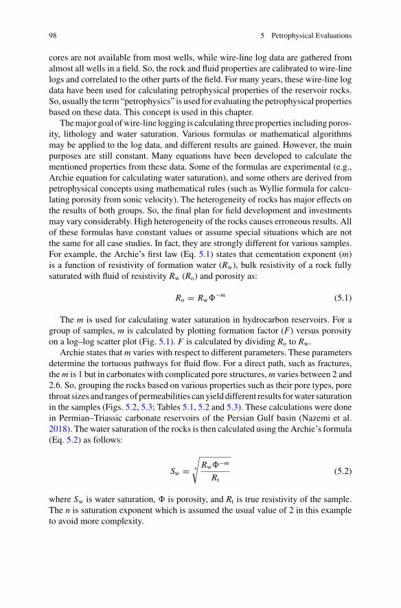
98 5 Petrophysical Evaluations
cores are not available from most wells, while wire-line log data are gathered fromalmost all wells in a field. So, the rock and fluid properties are calibrated to wire-linelogs and correlated to the other parts of the field. For many years, these wire-line logdata have been used for calculating petrophysical properties of the reservoir rocks.So, usually the term “petrophysics” is used for evaluating the petrophysical propertiesbased on these data. This concept is used in this chapter.
Themajor goal ofwire-line logging is calculating three properties includingporos-ity, lithology and water saturation. Various formulas or mathematical algorithmsmay be applied to the log data, and different results are gained. However, the mainpurposes are still constant. Many equations have been developed to calculate thementioned properties from these data. Some of the formulas are experimental (e.g.,Archie equation for calculating water saturation), and some others are derived frompetrophysical concepts using mathematical rules (such as Wyllie formula for calcu-lating porosity from sonic velocity). The heterogeneity of rocks has major effects onthe results of both groups. So, the final plan for field development and investmentsmay vary considerably. High heterogeneity of the rocks causes erroneous results. Allof these formulas have constant values or assume special situations which are notthe same for all case studies. In fact, they are strongly different for various samples.For example, the Archie’s first law (Eq. 5.1) states that cementation exponent (m)is a function of resistivity of formation water (Rw), bulk resistivity of a rock fullysaturated with fluid of resistivity Rw (Ro) and porosity as:
Ro = Rw�−m (5.1)
The m is used for calculating water saturation in hydrocarbon reservoirs. For agroup of samples, m is calculated by plotting formation factor (F) versus porosityon a log–log scatter plot (Fig. 5.1). F is calculated by dividing Ro to Rw.
Archie states thatm varies with respect to different parameters. These parametersdetermine the tortuous pathways for fluid flow. For a direct path, such as fractures,them is 1 but in carbonates with complicated pore structures,m varies between 2 and2.6. So, grouping the rocks based on various properties such as their pore types, porethroat sizes and ranges of permeabilities canyield different results forwater saturationin the samples (Figs. 5.2, 5.3; Tables 5.1, 5.2 and 5.3). These calculations were donein Permian–Triassic carbonate reservoirs of the Persian Gulf basin (Nazemi et al.2018). The water saturation of the rocks is then calculated using the Archie’s formula(Eq. 5.2) as follows:
Sw = n
√Rw�−m
Rt(5.2)
where Sw is water saturation, � is porosity, and Rt is true resistivity of the sample.The n is saturation exponent which is assumed the usual value of 2 in this exampleto avoid more complexity.
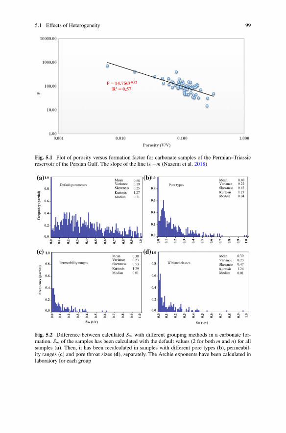
5.1 Effects of Heterogeneity 99
Fig. 5.1 Plot of porosity versus formation factor for carbonate samples of the Permian–Triassicreservoir of the Persian Gulf. The slope of the line is −m (Nazemi et al. 2018)
Fig. 5.2 Difference between calculated Sw with different grouping methods in a carbonate for-mation. Sw of the samples has been calculated with the default values (2 for both m and n) for allsamples (a). Then, it has been recalculated in samples with different pore types (b), permeabil-ity ranges (c) and pore throat sizes (d), separately. The Archie exponents have been calculated inlaboratory for each group
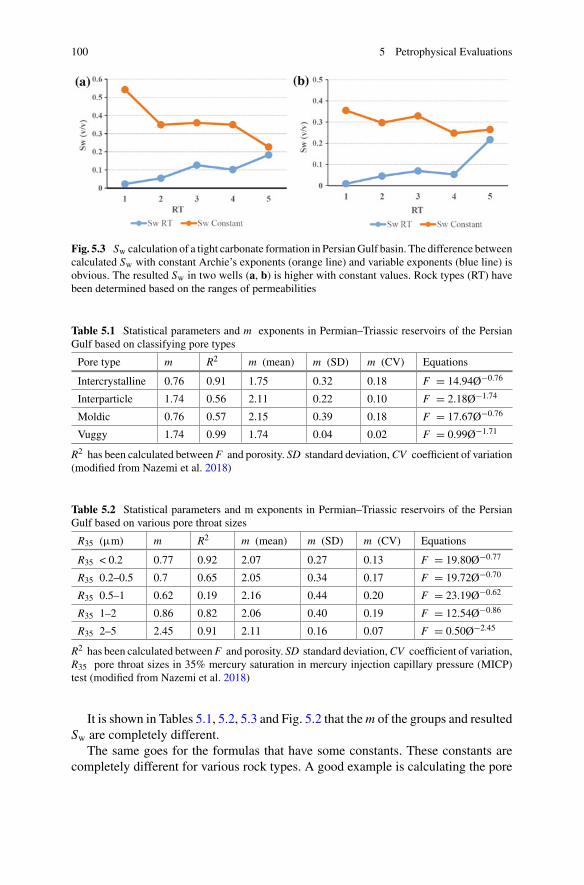
100 5 Petrophysical Evaluations
Fig. 5.3 Sw calculation of a tight carbonate formation in PersianGulf basin. The difference betweencalculated Sw with constant Archie’s exponents (orange line) and variable exponents (blue line) isobvious. The resulted Sw in two wells (a, b) is higher with constant values. Rock types (RT) havebeen determined based on the ranges of permeabilities
Table 5.1 Statistical parameters and m exponents in Permian–Triassic reservoirs of the PersianGulf based on classifying pore types
Pore type m R2 m (mean) m (SD) m (CV) Equations
Intercrystalline 0.76 0.91 1.75 0.32 0.18 F = 14.94Ø−0.76
Interparticle 1.74 0.56 2.11 0.22 0.10 F = 2.18Ø−1.74
Moldic 0.76 0.57 2.15 0.39 0.18 F = 17.67Ø−0.76
Vuggy 1.74 0.99 1.74 0.04 0.02 F = 0.99Ø−1.71
R2 has been calculated between F and porosity. SD standard deviation,CV coefficient of variation(modified from Nazemi et al. 2018)
Table 5.2 Statistical parameters and m exponents in Permian–Triassic reservoirs of the PersianGulf based on various pore throat sizes
R35 (µm) m R2 m (mean) m (SD) m (CV) Equations
R35 < 0.2 0.77 0.92 2.07 0.27 0.13 F = 19.80Ø−0.77
R35 0.2–0.5 0.7 0.65 2.05 0.34 0.17 F = 19.72Ø−0.70
R35 0.5–1 0.62 0.19 2.16 0.44 0.20 F = 23.19Ø−0.62
R35 1–2 0.86 0.82 2.06 0.40 0.19 F = 12.54Ø−0.86
R35 2–5 2.45 0.91 2.11 0.16 0.07 F = 0.50Ø−2.45
R2 has been calculated betweenF and porosity. SD standard deviation,CV coefficient of variation,R35 pore throat sizes in 35% mercury saturation in mercury injection capillary pressure (MICP)test (modified from Nazemi et al. 2018)
It is shown in Tables 5.1, 5.2, 5.3 and Fig. 5.2 that them of the groups and resultedSw are completely different.
The same goes for the formulas that have some constants. These constants arecompletely different for various rock types. A good example is calculating the pore
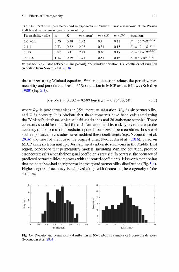
5.1 Effects of Heterogeneity 101
Table 5.3 Statistical parameters and m exponents in Permian–Triassic reservoirs of the PersianGulf based on various ranges of permeability
Permeability (mD) m R2 m (mean) m (SD) m (CV) Equations
0.01–0.1 0.30 0.98 1.92 0.4 0.21 F = 53.74Ø−0.30
0.1–1 0.73 0.62 2.03 0.31 0.15 F = 19.11Ø−0.73
1–10 0.92 0.31 2.23 0.40 0.18 F = 12.64Ø−0.92
10–100 1.12 0.89 1.91 0.31 0.16 F = 4.94Ø−1.12
R2 has been calculated between F and porosity. SD standard deviation,CV coefficient of variation(modified from Nazemi et al. 2018)
throat sizes using Winland equation. Winland’s equation relates the porosity, per-meability and pore throat sizes in 35% saturation in MICP test as follows (Kolodize1980) (Eq. 5.3):
log(R35) = 0.732+ 0.588 log(Kair) − 0.864 log(�) (5.3)
where R35 is pore throat sizes in 35% mercury saturation, Kair is air permeability,and � is porosity. It is obvious that these constants have been calculated usingthe Winland’s database which was 56 sandstones and 26 carbonate samples. Theseconstants should be modified for each formation and its rock types to increase theaccuracy of the formula for prediction pore throat sizes or permeabilities. In spite ofsuch importance, few studies have modified these coefficients (e.g., Nooruddin et al.2016) and most of them used the original ones. Nooruddin et al. (2016), based onMICP analysis from multiple Jurassic aged carbonate reservoirs in the Middle Eastregion, concluded that permeability models, including Winland equation, produceerroneous resultswhen their original coefficients are used. In contrast, the accuracy ofpredicted permeabilities improveswith calibrated coefficients. It is worthmentioningthat their database had nearly normal porosity andpermeability distribution (Fig. 5.4).Higher degree of accuracy is achieved along with decreasing heterogeneity of thesamples.
Fig. 5.4 Porosity and permeability distribution in 206 carbonate samples of Nooruddin database(Nooruddin et al. 2014)

102 5 Petrophysical Evaluations
5.2 Selecting the Parameters
Heterogeneity affects the petrophysical calculations, as discussed previously. So,the accuracy of formation evaluation results strongly depends on the appropriateselection of the parameters for these calculations. Two main approaches are usedto obtain the reservoir characteristics of any hydrocarbon formation. They includedeterministic and stochastic petrophysics. In deterministic approach, no randomnessis involved in the calculations and results. A deterministic formula always yields thesame result from a given starting condition or initial state. The user can change theformula or initial inputs. The result will be different, but it is always the same for thesame assumptions and equations. Volume of shale (V sh) calculation from gamma-ray(GR) log is a good example. In linear method, V sh is calculated using the followingformula (Eq. 5.4):
Vsh =(GRlog − GRmin
)/(GRmax − GRmin) (5.4)
where GRlog is the GR log reading at desired point, GRmin is the minimum GRvalue in the studied interval, and GRmax is its maximum. V sh of a point is always thesame using this equation. There are also some other formulas which can be used tocalculate the V sh, and so the result will be different but the value of this parameteris always constant using each formula. All of these formulas consider only a singleformation property and use one or at most two (e.g., V sh from neutron–density cross-plot) formation responses. A deterministic petrophysical approach uses a series ofstepwise calculations. For example, V sh is calculated based on the GR log data. Then,the shale effect is removed from the neutron responses using these data and porosityis determined. These two results are used to determine the volume of other mineralsin the reading point. The effects of other parameters are ignored in these calculations.For example, the response of the neutron tool can be affected by gypsum mineral orthe GR reading may be due to the K-feldspars or micas which are ignored in thesecalculations.
Some formation characteristics are selected in each step depend on the used for-mula. For example, for calculating the V sh, minimum and maximum amount of GRreadings are necessary. These constants may be simply the minimum and maximumof the GR data in whole interval, but the clay types may be different through thewhole reservoir part. So, different zones with different clay types should be definedto achieve realistic values.
Wyllie equation for calculating porosity from sonic velocity data is another exam-ple. He related these two parameters with a linear equation which is known asWyllietime–average equation (Eq. 5.5).
� = (�t − �tm)/(�tf − �tm) (5.5)
where � is porosity, �t is sonic transit time in true formation, �tm is sonic transittime in rock matrix, and �tf is sonic transit time in formation fluid.
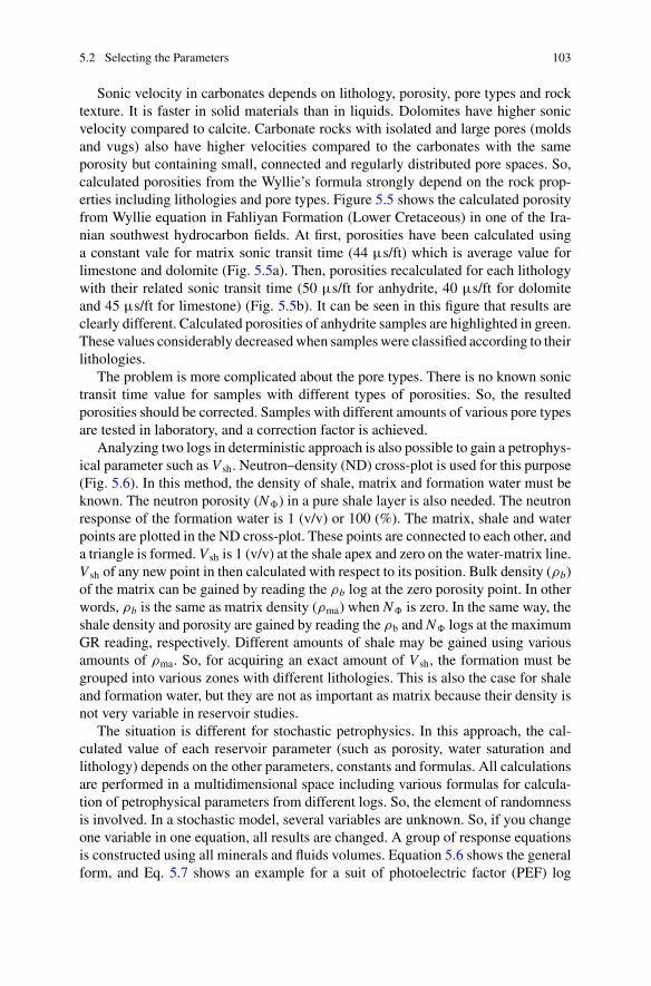
5.2 Selecting the Parameters 103
Sonic velocity in carbonates depends on lithology, porosity, pore types and rocktexture. It is faster in solid materials than in liquids. Dolomites have higher sonicvelocity compared to calcite. Carbonate rocks with isolated and large pores (moldsand vugs) also have higher velocities compared to the carbonates with the sameporosity but containing small, connected and regularly distributed pore spaces. So,calculated porosities from the Wyllie’s formula strongly depend on the rock prop-erties including lithologies and pore types. Figure 5.5 shows the calculated porosityfrom Wyllie equation in Fahliyan Formation (Lower Cretaceous) in one of the Ira-nian southwest hydrocarbon fields. At first, porosities have been calculated usinga constant vale for matrix sonic transit time (44 µs/ft) which is average value forlimestone and dolomite (Fig. 5.5a). Then, porosities recalculated for each lithologywith their related sonic transit time (50 µs/ft for anhydrite, 40 µs/ft for dolomiteand 45 µs/ft for limestone) (Fig. 5.5b). It can be seen in this figure that results areclearly different. Calculated porosities of anhydrite samples are highlighted in green.These values considerably decreasedwhen samples were classified according to theirlithologies.
The problem is more complicated about the pore types. There is no known sonictransit time value for samples with different types of porosities. So, the resultedporosities should be corrected. Samples with different amounts of various pore typesare tested in laboratory, and a correction factor is achieved.
Analyzing two logs in deterministic approach is also possible to gain a petrophys-ical parameter such as V sh. Neutron–density (ND) cross-plot is used for this purpose(Fig. 5.6). In this method, the density of shale, matrix and formation water must beknown. The neutron porosity (N�) in a pure shale layer is also needed. The neutronresponse of the formation water is 1 (v/v) or 100 (%). The matrix, shale and waterpoints are plotted in the ND cross-plot. These points are connected to each other, anda triangle is formed. V sh is 1 (v/v) at the shale apex and zero on the water-matrix line.V sh of any new point in then calculated with respect to its position. Bulk density (ρb)of the matrix can be gained by reading the ρb log at the zero porosity point. In otherwords, ρb is the same as matrix density (ρma) when N� is zero. In the same way, theshale density and porosity are gained by reading the ρb and N� logs at the maximumGR reading, respectively. Different amounts of shale may be gained using variousamounts of ρma. So, for acquiring an exact amount of V sh, the formation must begrouped into various zones with different lithologies. This is also the case for shaleand formation water, but they are not as important as matrix because their density isnot very variable in reservoir studies.
The situation is different for stochastic petrophysics. In this approach, the cal-culated value of each reservoir parameter (such as porosity, water saturation andlithology) depends on the other parameters, constants and formulas. All calculationsare performed in a multidimensional space including various formulas for calcula-tion of petrophysical parameters from different logs. So, the element of randomnessis involved. In a stochastic model, several variables are unknown. So, if you changeone variable in one equation, all results are changed. A group of response equationsis constructed using all minerals and fluids volumes. Equation 5.6 shows the generalform, and Eq. 5.7 shows an example for a suit of photoelectric factor (PEF) log
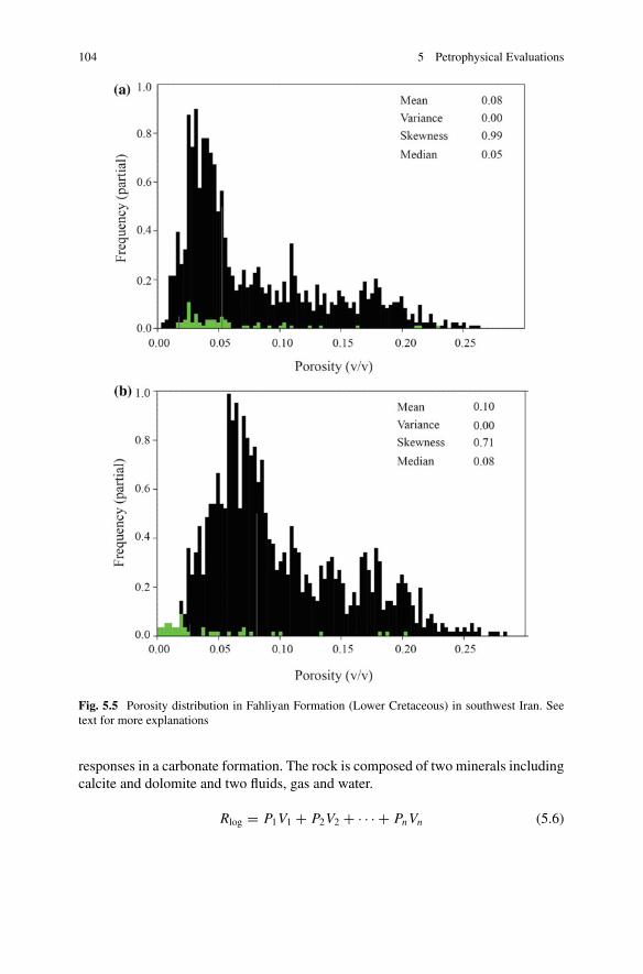
104 5 Petrophysical Evaluations
Fig. 5.5 Porosity distribution in Fahliyan Formation (Lower Cretaceous) in southwest Iran. Seetext for more explanations
responses in a carbonate formation. The rock is composed of two minerals includingcalcite and dolomite and two fluids, gas and water.
Rlog = P1V1 + P2V2 + · · · + PnVn (5.6)
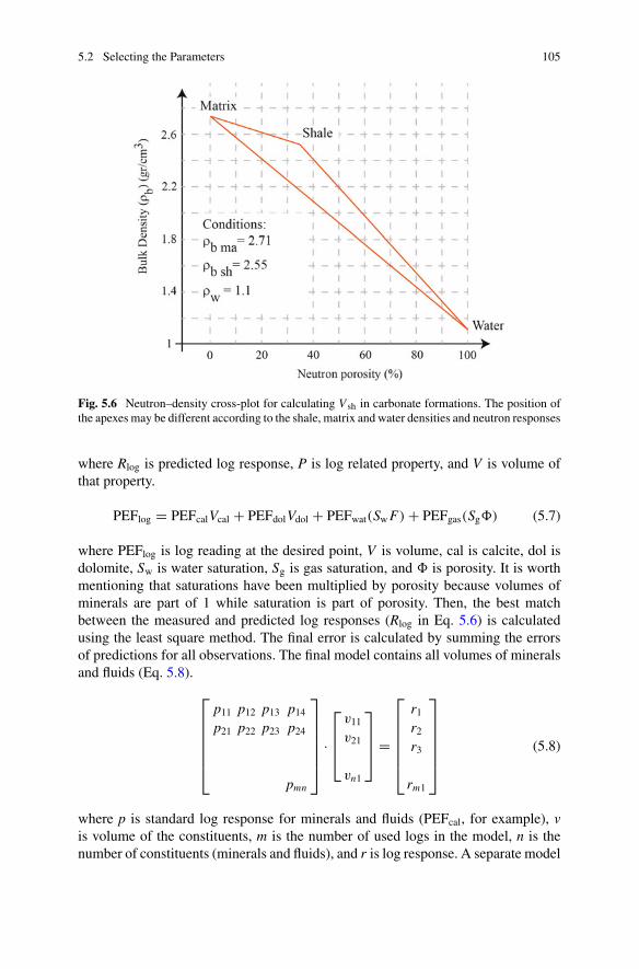
5.2 Selecting the Parameters 105
Fig. 5.6 Neutron–density cross-plot for calculating V sh in carbonate formations. The position ofthe apexes may be different according to the shale, matrix and water densities and neutron responses
where Rlog is predicted log response, P is log related property, and V is volume ofthat property.
PEFlog = PEFcalVcal + PEFdolVdol + PEFwat(SwF) + PEFgas(Sg�) (5.7)
where PEFlog is log reading at the desired point, V is volume, cal is calcite, dol isdolomite, Sw is water saturation, Sg is gas saturation, and � is porosity. It is worthmentioning that saturations have been multiplied by porosity because volumes ofminerals are part of 1 while saturation is part of porosity. Then, the best matchbetween the measured and predicted log responses (Rlog in Eq. 5.6) is calculatedusing the least square method. The final error is calculated by summing the errorsof predictions for all observations. The final model contains all volumes of mineralsand fluids (Eq. 5.8).
⎡⎢⎢⎢⎢⎢⎣
p11 p12 p13 p14p21 p22 p23 p24
pmn
⎤⎥⎥⎥⎥⎥⎦ ·
⎡⎢⎢⎣
v11
v21
vn1
⎤⎥⎥⎦ =
⎡⎢⎢⎢⎢⎢⎣
r1r2r3
rm1
⎤⎥⎥⎥⎥⎥⎦ (5.8)
where p is standard log response for minerals and fluids (PEFcal, for example), vis volume of the constituents, m is the number of used logs in the model, n is thenumber of constituents (minerals and fluids), and r is log response. A separate model
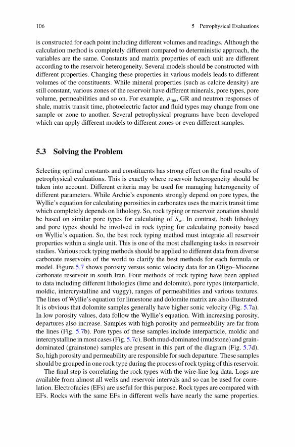
106 5 Petrophysical Evaluations
is constructed for each point including different volumes and readings. Although thecalculation method is completely different compared to deterministic approach, thevariables are the same. Constants and matrix properties of each unit are differentaccording to the reservoir heterogeneity. Several models should be constructed withdifferent properties. Changing these properties in various models leads to differentvolumes of the constituents. While mineral properties (such as calcite density) arestill constant, various zones of the reservoir have different minerals, pore types, porevolume, permeabilities and so on. For example, ρma, GR and neutron responses ofshale, matrix transit time, photoelectric factor and fluid types may change from onesample or zone to another. Several petrophysical programs have been developedwhich can apply different models to different zones or even different samples.
5.3 Solving the Problem
Selecting optimal constants and constituents has strong effect on the final results ofpetrophysical evaluations. This is exactly where reservoir heterogeneity should betaken into account. Different criteria may be used for managing heterogeneity ofdifferent parameters. While Archie’s exponents strongly depend on pore types, theWyllie’s equation for calculating porosities in carbonates uses the matrix transit timewhich completely depends on lithology. So, rock typing or reservoir zonation shouldbe based on similar pore types for calculating of Sw. In contrast, both lithologyand pore types should be involved in rock typing for calculating porosity basedon Wyllie’s equation. So, the best rock typing method must integrate all reservoirproperties within a single unit. This is one of the most challenging tasks in reservoirstudies. Various rock typing methods should be applied to different data from diversecarbonate reservoirs of the world to clarify the best methods for each formula ormodel. Figure 5.7 shows porosity versus sonic velocity data for an Oligo–Miocenecarbonate reservoir in south Iran. Four methods of rock typing have been appliedto data including different lithologies (lime and dolomite), pore types (interparticle,moldic, intercrystalline and vuggy), ranges of permeabilities and various textures.The lines of Wyllie’s equation for limestone and dolomite matrix are also illustrated.It is obvious that dolomite samples generally have higher sonic velocity (Fig. 5.7a).In low porosity values, data follow the Wyllie’s equation. With increasing porosity,departures also increase. Samples with high porosity and permeability are far fromthe lines (Fig. 5.7b). Pore types of these samples include interparticle, moldic andintercrystalline inmost cases (Fig. 5.7c). Bothmud-dominated (mudstone) and grain-dominated (grainstone) samples are present in this part of the diagram (Fig. 5.7d).So, high porosity and permeability are responsible for such departure. These samplesshould be grouped in one rock type during the process of rock typing of this reservoir.
The final step is correlating the rock types with the wire-line log data. Logs areavailable from almost all wells and reservoir intervals and so can be used for corre-lation. Electrofacies (EFs) are useful for this purpose. Rock types are compared withEFs. Rocks with the same EFs in different wells have nearly the same properties.
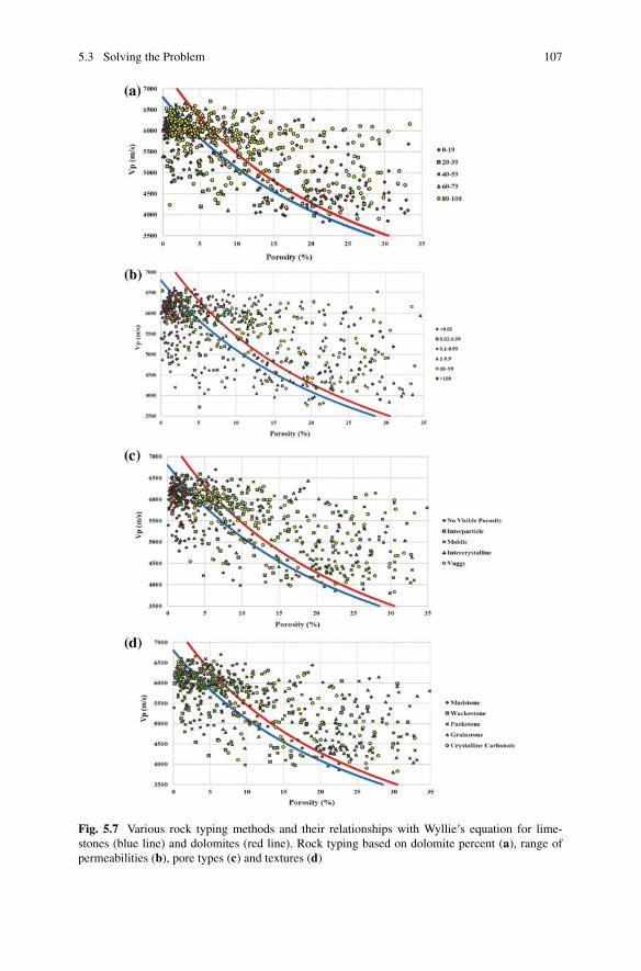
5.3 Solving the Problem 107
Fig. 5.7 Various rock typing methods and their relationships with Wyllie’s equation for lime-stones (blue line) and dolomites (red line). Rock typing based on dolomite percent (a), range ofpermeabilities (b), pore types (c) and textures (d)
108 5 Petrophysical Evaluations
So, the same constants and coefficients can be used for their petrophysical evalua-tion. These EFs are used for the final static reservoir modeling which indicates thedistribution of the properties in 3D space.
It should be mentioned that in all cases, the effect of overburden pressure mustbe involved in calculations. Both porosity and permeability decrease with increasingdepth and pressure. So, the estimated oil in place is always more than the real valuein the reservoir.
References
Kolodizie SJ (1980)Analysis of pore throat size and use of theWaxman-Smits equation to determineOOIP in Spindle Field, Colorado. SPE paper 9382 presented at the 1980 SPE Annual TechnicalConference and Exhibition, Dallas, Texas
Lucia FJ (2007) Carbonate reservoir characterization: an integrated approach. Springer, Berlin,Heidelberg
McPhee C, Reed J, Zubizarreta I (2015) Core analysis: a best practice guide. Elsevier, LondonNazemi M, Tavakoli V, Rahimpour-Bonab H, Hosseini M, Sharifi-Yazdi M (2018) The effect ofcarbonate reservoir heterogeneity on Archie’s exponents (a and m), an example fromKangan andDalan gas formations in the central Persian. Gulf J Nat Gas Sci Eng 59:297–308
Nooruddin HA, Hossain ME, Al-Yousef H, Okasha T (2014) Comparison of permeability modelsusing mercury injection capillary pressure data on carbonate rock samples. J Petrol Sci Eng12:9–22
Nooruddin HA, Hossain ME, Al-Yousef H, Okasha T (2016) Improvement of permeability modelsusing large mercury injection capillary pressure dataset for middle east carbonate reservoirs. JPorous Media 19(5):405–422
Tavakoli (2018) Geological core analysis: application to reservoir characterization. Springer, ChamTiab D, Donaldson EC (2015) Petrophysics, theory and practice of measuring reservoir rock andfluid transport properties. Gulf Professional Publishing, Houston


![[IJCT-V1I2P2] Author :Vahid Ghoreish](https://img.pdfslide.us/doc/110x75/577cc1761a28aba7119326b7/ijct-v1i2p2-author-vahid-ghoreish.jpg)


![[Hossein Tavakoli] a Dictionary of Research Method(BookFi.org)](https://img.pdfslide.us/doc/110x75/55cf9504550346f57ba5fa6a/hossein-tavakoli-a-dictionary-of-research-methodbookfiorg.jpg)