Embed Size (px)
Citation preview
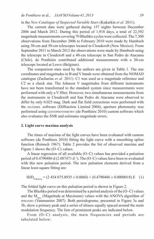
de Ponthiere et al., JAAVSO Volume 41, 201358
V1820 Orionis: an RR Lyrae Star With Strong and Irregular Blazhko Effect
Pierre de Ponthière15 Rue Pré Mathy, Lesve, Profondeville 5170, Belgium; [email protected]
Franz-Josef (Josch) Hambsch12 Oude Bleken, Mol, 2400, Belgium; [email protected]
Tom KrajciP.O. Box 1351, Cloudcroft, NM 88317; [email protected]
Kenneth Menzies318A Potter Road, Framingham, MA, 01701
Patrick WilsAarschotsebaan 31, Hever B-3191, Belgium; [email protected]
Received October 12, 2012; revised November 27, 2012; accepted November 29, 2012
Abstract The Blazhko effect in V1820 Orionis and its period were reported for the first time by Wils et al. (MNRAS, 368, 1757; 2006) from a data analysis of the Northern Sky Variability Survey. The results of additional V1820 Orionis observations over a time span of four years are presented herein. From the observed light curves, 73 pulsation maxima have been measured. The times of light maxima have been compared to ephemerides to obtain the (O–C) values. The Blazhko period (27.917 ± 0.002 d) has been derived from light curve Fourier analysis and from ANOVA analyses of the (O–C) values and of magnitudes at maximum light (Mmax). During one Blazhko cycle, a hump in the ascending branch of the light curve was clearly identified and has also created a double maximum in the light curve. The frequency spectrum of the light curve, from a Fourier analysis with period04, has revealed triplet, quintuplet structures, and a second Blazhko weak modulation (period = 34.72 ±0.01 d). V1820 Orionis can be ranked as a strongly modulated star based on its observed amplitude and phase variations. The amplitude ratio of the largest triplet component to main pulsation component is quite large: 0.34.
1. Introduction
The star V1820 Orionis is classified in the General Catalogue of Variable Stars (Samus et al. 2011) as an RR Lyr (RRab) variable star with a period of 0.479067 day and with maximum and minimum V-band magnitudes of 12.5 and 13.4, respectively. This star was identified as an RRab with a Blazhko period of 28 days by Wils et al. (2006). At this time the star was classified as NSV 02724
de Ponthiere et al., JAAVSO Volume 41, 2013 59
in the New Catalogue of Suspected Variable Stars (Kukarkin et al. 2011). The current data were gathered during 157 nights between December 2006 and March 2012. During this period of 1,918 days, a total of 22,592 magnitude measurements covering 70 Blazhko cycles were collected. The 7,300 observations from December 2006 to February 2010 were made by Hambsch using 30-cm and 50-cm telescopes located in Cloudcroft (New Mexico). From September 2011 to March 2012 the observations were made by Hambsch using the telescope in Cloudcroft and a 40-cm telescope in San Pedro de Atacama (Chile). de Ponthière contributed additional measurements with a 20-cm telescope located at Lesve (Belgium). The comparison stars used by the authors are given in Table 1. The star coordinates and magnitudes in B and V bands were obtained from the NOMAD catalogue (Zacharias et al. 2011). C1 was used as a magnitude reference and C2 as a check star. The Johnson V magnitudes from different instruments have not been transformed to the standard system since measurements were performed with only a V filter. However, two simultaneous measurements from the instruments in Cloudcroft and San Pedro de Atacama were observed to differ by only 0.025 mag. Dark and flat field corrections were performed with the maximdl software (Diffraction Limited 2004), aperture photometry was performed using lesvephotometry (de Ponthière 2010) custom software which also evaluates the SNR and estimates magnitude errors.
2. Light curve maxima analysis
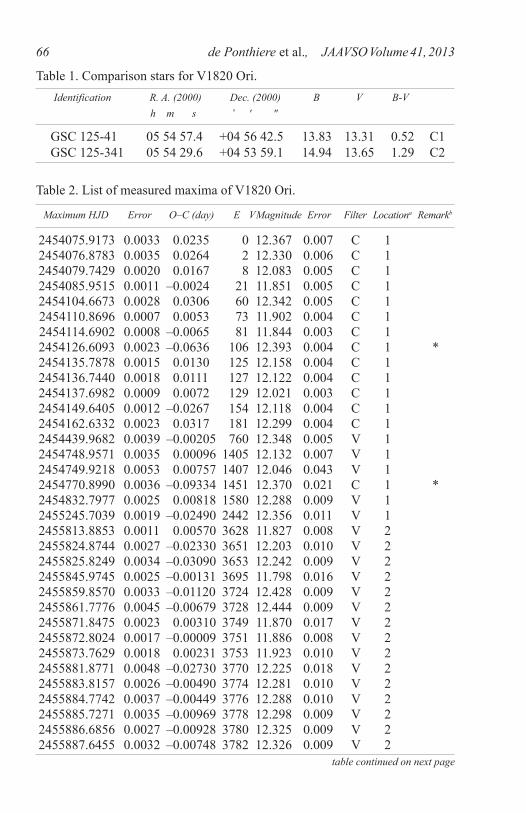
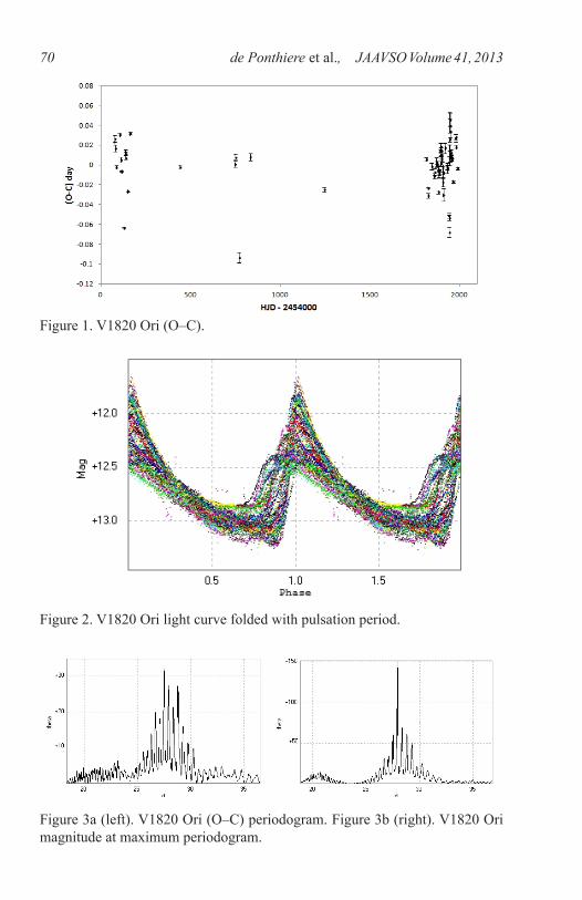
The times of maxima of the light curves have been evaluated with custom software (de Ponthiere 2010) fitting the light curve with a smoothing spline function (Reinsch 1967). Table 2 provides the list of observed maxima and Figure 1 shows the (O–C) values. A linear regression of all available (O–C) values has provided a pulsation period of 0.4790486 d (2.087471 d–1). The (O–C) values have been re-evaluated with this new pulsation period. The new pulsation elements derived from a linear least-square fitting are:
HJDPulsation = (2 454 075.8935 ± 0.0060) + (0.4790486 ± 0.0000018) E (1)
The folded light curve on this pulsation period is shown in Figure 2. The Blazhko period was determined by a period analysis of the (O–C) values and the Mmax (Magnitude at Maximum) values with the ANOVA algorithm of peranso (Vanmunster 2007). Both periodograms, presented in Figure 3a and 3b, show a primary peak and a series of aliases equally spaced around the main modulation frequency. The lists of prominent peaks are indicated below. From (O–C) analysis, the main frequencies and periods are tabulated below:
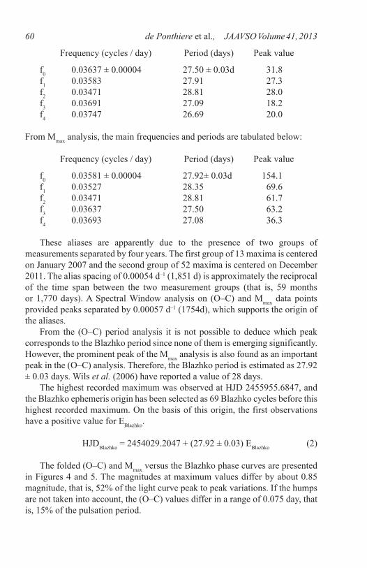
de Ponthiere et al., JAAVSO Volume 41, 201360
Frequency (cycles / day) Period (days) Peak value
f0 0.03637 ± 0.00004 27.50 ± 0.03d 31.8 f1 0.03583 27.91 27.3 f2 0.03471 28.81 28.0 f3 0.03691 27.09 18.2 f4 0.03747 26.69 20.0
From Mmax analysis, the main frequencies and periods are tabulated below:
Frequency (cycles / day) Period (days) Peak value
f0 0.03581 ± 0.00004 27.92± 0.03d 154.1 f1 0.03527 28.35 69.6 f2 0.03471 28.81 61.7 f3 0.03637 27.50 63.2 f4 0.03693 27.08 36.3
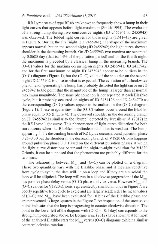
These aliases are apparently due to the presence of two groups of measurements separated by four years. The first group of 13 maxima is centered on January 2007 and the second group of 52 maxima is centered on December 2011. The alias spacing of 0.00054 d–1 (1,851 d) is approximately the reciprocal of the time span between the two measurement groups (that is, 59 months or 1,770 days). A Spectral Window analysis on (O–C) and Mmax data points provided peaks separated by 0.00057 d–1 (1754d), which supports the origin of the aliases. From the (O–C) period analysis it is not possible to deduce which peak corresponds to the Blazhko period since none of them is emerging significantly. However, the prominent peak of the Mmax analysis is also found as an important peak in the (O–C) analysis. Therefore, the Blazhko period is estimated as 27.92 ± 0.03 days. Wils et al. (2006) have reported a value of 28 days. The highest recorded maximum was observed at HJD 2455955.6847, and the Blazhko ephemeris origin has been selected as 69 Blazhko cycles before this highest recorded maximum. On the basis of this origin, the first observations have a positive value for EBlazhko.
HJDBlazhko = 2454029.2047 + (27.92 ± 0.03) EBlazhko (2)
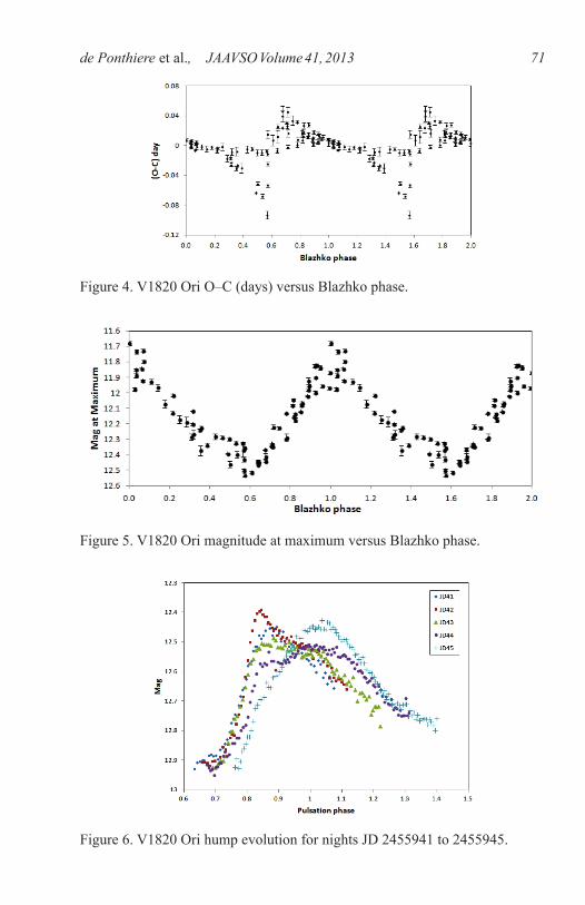
The folded (O–C) and Mmax versus the Blazhko phase curves are presented in Figures 4 and 5. The magnitudes at maximum values differ by about 0.85 magnitude, that is, 52% of the light curve peak to peak variations. If the humps are not taken into account, the (O–C) values differ in a range of 0.075 day, that is, 15% of the pulsation period.
de Ponthiere et al., JAAVSO Volume 41, 2013 61
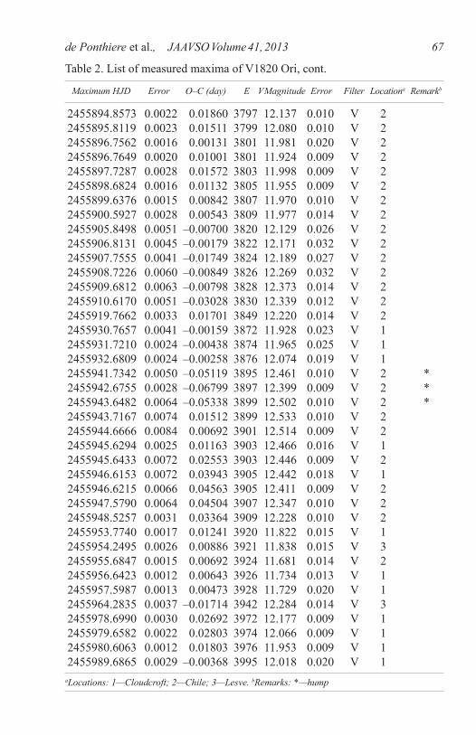
RR Lyrae stars of type RRab are known to frequently show a hump in their light curves that appears before light maximum (Smith 1995). The evolution of a strong hump during five consecutive nights (JD 2455941 to 2455945) was observed. The folded light curves for those nights (JD41–45) are given in Figure 6. During the first night (JD 2455941), the shape of the maximum appears normal, but on the second night (JD 2455942) the light curve shows a shoulder in the decreasing branch. On JD 2455943 two maxima are separated by 0.0685 day (that is, 14% of the pulsation period) and on the fourth night, the maximum is preceded by a classical hump in the increasing branch. The (O–C) values for the maxima occurring on nights JD 2455941, JD 2455942, and for the first maximum on night JD 2455943 appear to be outliers in the (O–C) diagram (Figure 1), but the (O–C) value of the shoulder on the second night JD 2455942 is close to what is expected. The evolution of a shockwave phenomenon generating the hump has probably distorted the light curve on JD 2455942 to the point that the magnitude of the hump is larger than at normal maximum magnitude. The same phenomenon is not repeated at each Blazhko cycle, but it probably occurred on nights of JD 2454126 and JD 2454770 as the corresponding (O–C) values appear to be outliers in the (O–C) diagram (Figure 1). These irregularities in the (O–C) values occur around the Blazhko phase equal to 0.5 (Figure 4). The observed shoulder in the decreasing branch on JD 2455942 is similar to the “bump” detected by Jurcsik et al. (2012) in the RZ Lyrae light curve. This phenomenon of light curve distortion for both stars occurs when the Blazhko amplitude modulation is weakest. The bump appearing in the descending branch of RZ Lyrae occurs around pulsation phase 0.25–0.30 but the shoulder in the decreasing branch of V1820 Orionis happens around pulsation phase 0.0. Based on the different pulsation phases at which the light curve distortions occur and the night-to-night evolution for V1820 Orionis, it can be supposed that the phenomena are probably different for the two stars. The relationship between Mmax and (O–C) can be plotted on a diagram. These two quantities vary with the Blazhko phase and if they are repetitive from cycle to cycle, the data will lie on a loop and if they are sinusoidal the loop will be elliptical. The loop will run in a clockwise progression if the Mmax has positive phase delay versus (O–C) phase and vice-versa. However Mmax and (O–C) values for V1820 Orionis, represented by small diamonds in Figure 7, are poorly repetitive from cycle to cycle and are largely scattered. The mean values of (O–C) and Mmax have been evaluated for 10 bins of the Blazhko phase and are represented as large squares in the Figure 7. An inspection of the successive points indicates that the loop is progressing in counter-clockwise direction. The point in the lower left of the diagram with (O–C = –0.1 day) corresponds to the strong hump described above. Le Borgne et al. (2012) have shown that for most of the analyzed Blazhko stars the Mmax versus (O–C) diagrams exhibit a similar counterclockwise rotation.
de Ponthiere et al., JAAVSO Volume 41, 201362
3. Frequency spectrum analysis
A Blazhko effect on the light curve can be modeled as an amplitude and/or phase modulation of the periodic pulsation, with the reciprocal of the modulation frequency being the Blazhko period. Szeidl and Jurcsik (2009) have shown that the Fourier spectrum of an amplitude and phase modulation model is given by an infinite series including the fundamental frequency (f0), harmonic frequencies (if0), and multiplet frequencies (if0 ± jfB).
m(t) = Σ Ai sin(iωt + Φi0) + ΣΣ A+ij sin[(iω + jΩ)t + Φ+
ij] + ΣΣ A–
ij sin[(iω – jΩ)t + Φ–ij] (3)
where:
ω = 2πf0, f0 is the fundamental frequency of the light-curve,Ω = 2πfB, fB is the Blazhko modulation frequency, andAi A
+ ij A–ij are the Fourier coefficients and Φi, Φ
+ij and Φ–
ij j their phase angles, “i” indices are used for the fundamental and the harmonic frequencies and “j” indices for the side lobes (for example, A+
32 is the coefficient of the multiplet (3f0 + 2fB) .
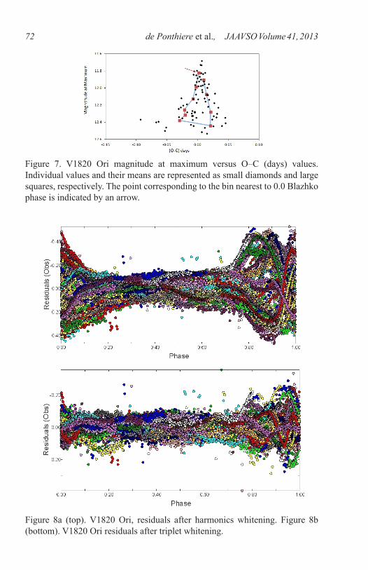
The methodology used herein is similar to the one reported by Kolenberg (2009) where triplet and quintuplet components were detected in the spectrum of SS Fornacis. The spectral analysis was performed with period04 (Lenz and Breger 2005) to yield a Fourier analysis and multi-frequency sine-wave fitting. The sine-wave fitting was determined by successive data pre-whitening and Fourier analysis on residuals. For each observed harmonic and triplet, the signal-to-noise ratio has been evaluated to retain only significant signals, that is, with an SNR greater than 3.5. During the period04 sine-wave fitting process, only the fundamental f0 and the first main triplet component f0 + fB frequencies have been unconstrained; the other frequencies have been entered as combinations of f0 and f0 + fB. Table 3 provides the amplitude and phase for each Fourier component obtained with the best sine-wave fitting. The uncertainties of frequencies, amplitudes, and phases have been estimated by Monte Carlo simulations. As it is known that Monte Carlo simulation uncertainties can be underestimated (Kolenberg et al. 2009), the uncertainty values have been multiplied by a factor of two. The harmonics of f0 are significant to the eighth order. The residuals after subtraction of the best fit based on f0 and harmonics up to the eighth order is provided in Figure 8a. The large residuals close to the phase of maximum light (0.8 to 1.1) are due to amplitude and phase modulations created by the Blazhko effect. The residuals are reduced significantly when the side peaks (triplets) around the f0 frequency and harmonics up to the seventh order are included in the fitting process (Figure 8b). The fundamental pulsation frequency f0 (2.08747 d–1) is very close to the frequency obtained from a linear regression analysis of time of maxima. The
de Ponthiere et al., JAAVSO Volume 41, 2013 63
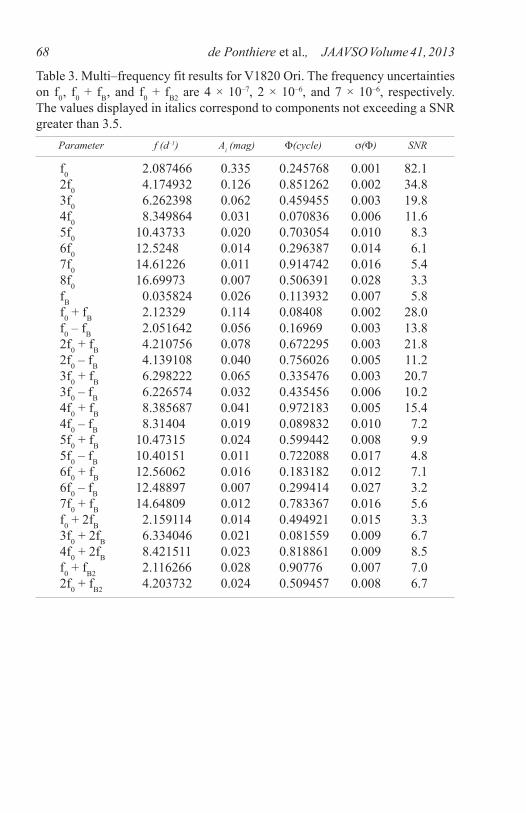
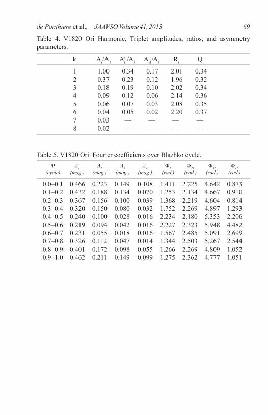
Blazhko period was also measured from the first side peak frequency f0 + fB and f0 to yield fB = (2.12329 – 2.08747) = 0.03582 d–1 and PB = 27.917 ± 0.002 days. The second side peak frequency f0 – fB exhibited a lower amplitude and higher uncertainty and was not used for Blazhko period evaluation. The Blazhko period found with the sine-wave fitting method (27.919 ± 0.002 days) is equal to the value found with the brightness at maximum analysis (27.92 ± 0.03 days). Table 4 lists the harmonic and significant amplitude ratios. One useful parameter to quantify the Blazhko effect is the amplitude ratio A±
11 / A1, where A±
11 is the amplitude of the largest side lobe at f0 + fB or f0 – fB and A1 is the amplitude of f0. The most common and maximum values for this ratio are 0.15 and 0.4, respectively (Alcock et al. 2003). With an amplitude ratio A11
+ / A1 = 0.34, V1820 Orionis can be ranked as strongly modulated. The triplet ratios Ri = A+
i1 / A–i1 and asymmetries Qi = (A+
i1 – A–i1) / (A
+i1 +
A–i1) are also provided in Table 4. The asymmetry in the side lobes observed
for V1820 Orionis is not unexpected on the basis of Szeidl and Jurcsik (2009), which showed that this asymmetry is related to the phase difference between the Blazhko amplitude and phase modulations. If the Blazhko effect were limited to amplitude modulation, the ratios Ri and Qi would be equal to 1 and 0, respectively. The asymmetry ratios Qi around 0.35 are a sign that V1820 Orionis is amplitude- and phase-modulated. Besides the harmonics and triplets, some quintuplet components (kf0 + 2fB) and a peak at the Blazhko period itself were found. And finally, two modulation peaks appear in the spectrum around f0 and 2f0 with a separation of 0.028 d–
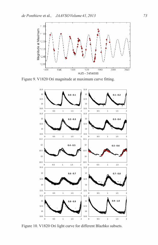
1. They correspond to a second Blazhko modulation fB2 (1/fB2 = 34.72 ± 0.01 days). This phenomenon of multi-periodic modulation has also been detected by Sódor et al. (2011) in the spectrum of CZ Lacertae. In the case of CZ Lac, the modulation components of the two frequencies (fB and fB2) have similar amplitudes, which is not the case for V1820 Orionis. The second modulation frequency fB2 has weaker components than fB, but they remain significant as their SNR are 9.2 and 6.0, respectively. A spectral analysis on Mmax values provides the same two Blazhko modulation frequencies fB and fB2, which are in a 5:4 resonance ratio. The corresponding beating period is 139 days, which is visible on the multi-frequency sine-wave fitting obtained with period04 (Figure 9). For clarity, Figure 9 only includes the last observation season (2011–2012). A 5:4 resonance ratio was also found between the two modulation frequencies of CZ Lac during the 2004 observation season (Sódor et al. 2011) but the next year this resonance ratio changed to a value of 4:3.
4. Light curve variations over Blazhko cycle
In order to investigate the light curve variations over the Blazhko cycle, the complete dataset was subdivided into ten temporal subsets corresponding to different Blazhko phase intervals Ψi (i = 0,9). The ephemeris derived previously
de Ponthiere et al., JAAVSO Volume 41, 201364
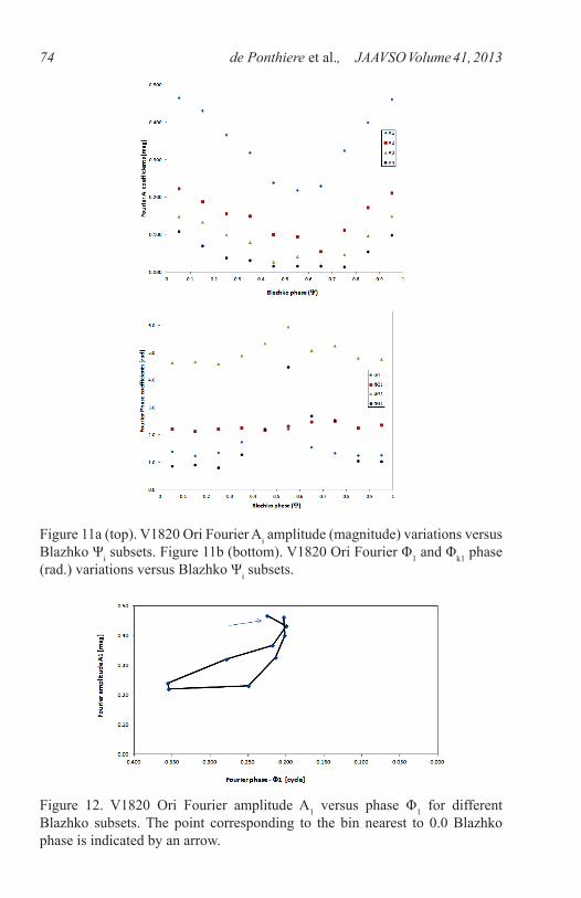
during the analysis of light curve maxima was used to define the epoch of the Blazhko zero phase (HJD = 2454029.2047). The data points are relatively well distributed over the subsets with the number of data points in each subset varying between 1,144 and 3,045. The light curves for each subset are presented in Figure 10. The strong hump observed during JD 2455942, as described previously, is highlighted in red in the panel of subset ( Ψ = 0.5–0.6). For each subset, the amplitude Ai and phase Φi of of the fundamental and harmonic frequencies up to the fourth order have been evaluated with the Least-Square Fit module of period04. The amplitudes and epoch-independent phase differences (Φk1 = Φk – kΦ1) over the Blazhko cycle are provided in Table 4 and exhibited in Figures 11a and 11b. As expected, the amplitude of the fundamental frequency is clearly lower at a Blazhko phase around 0.5, that is, when the light curve amplitude variation on the pulsation cycle is weaker. The maximum and minimum Φ1 phase values (2.234 and 1.253 radians) are found in subsets Ψ (0.4–0.5) and Ψ (0.1–0.2), respectively. The difference between maximum and minimum Φ1 phase is a measure of the phase modulation strength and is equal to (2.234 – 1.253) = 0.981 radian or 0.156 cycle, which corresponds roughly to the value of 15 % noted for the peak to peak deviation of (O–C). The phase variation of harmonic component Φ41 is the largest, with a value of 3.6 radians, while Φ21 varies only by 0.37 radians over the Blazhko cycle. The phase variation of harmonic component Φ41 is very large as compared to Φk1 values of 1 and 0.5 radians observed for RZ Lyrae (Jurcsik et al. 2012) and SS Fornacis (Kolenberg et al. 2009), respectively. Figure 12 provides a graph of the A1 coefficient versus the Φ1 for the different subsets. This graph is similar to the graph of the Magnitude at Maximum versus (O–C) given in Figure 7. In order to compare the two graphs, the Φ1 axis of Figure 12 was inverted. Indeed, for the sine-wave fitting [Ai sin(ωi t + Φi)], a larger Φi phase corresponds to a time advance, that is, a lower value of (O–C). With the Φ1 axis inverted, the loop of A1 values exhibits a counter-clockwise progression as in Figure 7.
5. Conclusions
The strong and irregular Blazhko behavior of V1820 Ori has been exhibited by two different methods: (1) measurement of light curve maxima, and (2) Fourier analysis. The latter method, Fourier analysis, has been feasible due to the large number of regular observations over the pulsation period which was not limited to the times of light curve maxima. Both methods yield the same results for the fundamental pulsation period (0.4790486 day ± 0.0000018) and the Blazhko period (27.917 days ± 0.002). The irregularities of the Blazhko effect are probably explained by variations of the strength of a shockwave phenomenon generating the hump in the ascending branch of the light curve. This erratic behavior generally occurs around a Blazhko phase of 0.5. Measured
de Ponthiere et al., JAAVSO Volume 41, 2013 65
ratios of Fourier amplitudes and their asymmetries also confirm strong Blazhko amplitude and phase modulations. A second weaker Blazhko modulation with a period 34.70 ±0.02 days has also been identified. The two modulation frequencies are in a 5:4 resonance ratio.
6. Acknowledgements
Dr. Arne Henden, Director of AAVSO, and the AAVSO are acknowledged for the use of AAVSOnet telescopes at Cloudcroft, New Mexico. The authors thank Dr. Katrien Kolenberg for helpful suggestions in the Fourier analysis and the referee Dr. Johanna Jurcsik for constructive comments which have helped to clarify and improve the paper.
References
Alcock, C., et al. 2003, Astrophys. J., 598, 597.de Ponthière, P. 2010, lesvephotometry, automatic photometry software (http://
www.dppobservatory.net). Diffraction Limited. 2004, maximdl image processing software (http://www.
cyanogen.com).Jurcsik, J., et al. 2012, Mon. Not. Roy. Astron. Soc., 423, 993.Kolenberg, K., et al. 2009, Mon. Not. Roy. Astron. Soc., 396, 263.Kukarkin, B., et al. 2011, New Catalogue of Suspected Variable Sars (NSV
database, Version 2011 March, http://www.sai.msu.su/gcvs/gcvs/nsv/nsv.dat).
Le Borgne, J. F., et al. 2012, Astron. J., 144, 39.Lenz, P., and Breger, M. 2005, Commun. Asteroseismology, 146, 53.Reinsch, C. H. 1967, Numer. Math., 10, 177.Samus, N. N., et al. 2011 General Catalogue of Variable Stars (GCVS database,
Version 2011 January, http://www.sai.msu.su/gcvs/gcvs/index.htm).Smith, H. 1995, RR Lyrae Stars, Cambridge Univ. Press, Cambridge.Sódor, Á., et al. 2011, Mon. Not. Roy. Astron. Soc., 411, 1585.Szeidl, B., and Jurcsik, J. 2009 Commun. Asteroseismology, 160, 17.Vanmunster, T. 2007, peranso, period analysis software (http://www.cbabelgium.
com and http://www.peranso.com).Wils, P., Lloyd, C., and Bernhard, K. 2006, Mon. Not. Roy. Astron. Soc., 368, 1757.Zacharias, N., Monet, D., Levine, S., Urban, S., Gaume, R., and Wycoff, G.
2011, The Naval Observatory Merged Astrometric Dataset (NOMAD, http://www.usno.navy.mil/USNO/astrometry/optical-IR-prod/nomad/).
de Ponthiere et al., JAAVSO Volume 41, 201366
Table 1. Comparison stars for V1820 Ori. Identification R. A. (2000) Dec. (2000) B V B-V h m s ˚ ' "
GSC 125-41 05 54 57.4 +04 56 42.5 13.83 13.31 0.52 C1 GSC 125-341 05 54 29.6 +04 53 59.1 14.94 13.65 1.29 C2
2454075.9173 0.0033 0.0235 0 12.367 0.007 C 1 2454076.8783 0.0035 0.0264 2 12.330 0.006 C 1 2454079.7429 0.0020 0.0167 8 12.083 0.005 C 1 2454085.9515 0.0011 –0.0024 21 11.851 0.005 C 1 2454104.6673 0.0028 0.0306 60 12.342 0.005 C 1 2454110.8696 0.0007 0.0053 73 11.902 0.004 C 1 2454114.6902 0.0008 –0.0065 81 11.844 0.003 C 1 2454126.6093 0.0023 –0.0636 106 12.393 0.004 C 1 * 2454135.7878 0.0015 0.0130 125 12.158 0.004 C 1 2454136.7440 0.0018 0.0111 127 12.122 0.004 C 1 2454137.6982 0.0009 0.0072 129 12.021 0.003 C 1 2454149.6405 0.0012 –0.0267 154 12.118 0.004 C 1 2454162.6332 0.0023 0.0317 181 12.299 0.004 C 1 2454439.9682 0.0039 –0.00205 760 12.348 0.005 V 1 2454748.9571 0.0035 0.00096 1405 12.132 0.007 V 1 2454749.9218 0.0053 0.00757 1407 12.046 0.043 V 1 2454770.8990 0.0036 –0.09334 1451 12.370 0.021 C 1 * 2454832.7977 0.0025 0.00818 1580 12.288 0.009 V 1 2455245.7039 0.0019 –0.02490 2442 12.356 0.011 V 1 2455813.8853 0.0011 0.00570 3628 11.827 0.008 V 2 2455824.8744 0.0027 –0.02330 3651 12.203 0.010 V 2 2455825.8249 0.0034 –0.03090 3653 12.242 0.009 V 2 2455845.9745 0.0025 –0.00131 3695 11.798 0.016 V 2 2455859.8570 0.0033 –0.01120 3724 12.428 0.009 V 2 2455861.7776 0.0045 –0.00679 3728 12.444 0.009 V 2 2455871.8475 0.0023 0.00310 3749 11.870 0.017 V 2 2455872.8024 0.0017 –0.00009 3751 11.886 0.008 V 2 2455873.7629 0.0018 0.00231 3753 11.923 0.010 V 2 2455881.8771 0.0048 –0.02730 3770 12.225 0.018 V 2 2455883.8157 0.0026 –0.00490 3774 12.281 0.010 V 2 2455884.7742 0.0037 –0.00449 3776 12.288 0.010 V 2 2455885.7271 0.0035 –0.00969 3778 12.298 0.009 V 2 2455886.6856 0.0027 –0.00928 3780 12.325 0.009 V 2 2455887.6455 0.0032 –0.00748 3782 12.326 0.009 V 2
Table 2. List of measured maxima of V1820 Ori.
Maximum HJD Error O–C (day) E V Magnitude Error Filter Locationa Remarkb
table continued on next page
de Ponthiere et al., JAAVSO Volume 41, 2013 67
2455894.8573 0.0022 0.01860 3797 12.137 0.010 V 2 2455895.8119 0.0023 0.01511 3799 12.080 0.010 V 2 2455896.7562 0.0016 0.00131 3801 11.981 0.020 V 2 2455896.7649 0.0020 0.01001 3801 11.924 0.009 V 2 2455897.7287 0.0028 0.01572 3803 11.998 0.009 V 2 2455898.6824 0.0016 0.01132 3805 11.955 0.009 V 2 2455899.6376 0.0015 0.00842 3807 11.970 0.010 V 2 2455900.5927 0.0028 0.00543 3809 11.977 0.014 V 2 2455905.8498 0.0051 –0.00700 3820 12.129 0.026 V 2 2455906.8131 0.0045 –0.00179 3822 12.171 0.032 V 2 2455907.7555 0.0041 –0.01749 3824 12.189 0.027 V 2 2455908.7226 0.0060 –0.00849 3826 12.269 0.032 V 2 2455909.6812 0.0063 –0.00798 3828 12.373 0.014 V 2 2455910.6170 0.0051 –0.03028 3830 12.339 0.012 V 2 2455919.7662 0.0033 0.01701 3849 12.220 0.014 V 2 2455930.7657 0.0041 –0.00159 3872 11.928 0.023 V 1 2455931.7210 0.0024 –0.00438 3874 11.965 0.025 V 1 2455932.6809 0.0024 –0.00258 3876 12.074 0.019 V 1 2455941.7342 0.0050 –0.05119 3895 12.461 0.010 V 2 * 2455942.6755 0.0028 –0.06799 3897 12.399 0.009 V 2 * 2455943.6482 0.0064 –0.05338 3899 12.502 0.010 V 2 * 2455943.7167 0.0074 0.01512 3899 12.533 0.010 V 2 2455944.6666 0.0084 0.00692 3901 12.514 0.009 V 2 2455945.6294 0.0025 0.01163 3903 12.466 0.016 V 1 2455945.6433 0.0072 0.02553 3903 12.446 0.009 V 2 2455946.6153 0.0072 0.03943 3905 12.442 0.018 V 1 2455946.6215 0.0066 0.04563 3905 12.411 0.009 V 2 2455947.5790 0.0064 0.04504 3907 12.347 0.010 V 2 2455948.5257 0.0031 0.03364 3909 12.228 0.010 V 2 2455953.7740 0.0017 0.01241 3920 11.822 0.015 V 1 2455954.2495 0.0026 0.00886 3921 11.838 0.015 V 3 2455955.6847 0.0015 0.00692 3924 11.681 0.014 V 2 2455956.6423 0.0012 0.00643 3926 11.734 0.013 V 1 2455957.5987 0.0013 0.00473 3928 11.729 0.020 V 1 2455964.2835 0.0037 –0.01714 3942 12.284 0.014 V 3 2455978.6990 0.0030 0.02692 3972 12.177 0.009 V 1 2455979.6582 0.0022 0.02803 3974 12.066 0.009 V 1 2455980.6063 0.0012 0.01803 3976 11.953 0.009 V 1 2455989.6865 0.0029 –0.00368 3995 12.018 0.020 V 1
Table 2. List of measured maxima of V1820 Ori, cont.
Maximum HJD Error O–C (day) E V Magnitude Error Filter Locationa Remarkb
aLocations: 1—Cloudcroft; 2—Chile; 3—Lesve. bRemarks: *—hump
de Ponthiere et al., JAAVSO Volume 41, 201368
Table 3. Multi–frequency fit results for V1820 Ori. The frequency uncertainties on f0, f0 + fB, and f0 + fB2 are 4 × 10⁻⁷, 2 × 10⁻⁶, and 7 × 10⁻⁶, respectively. The values displayed in italics correspond to components not exceeding a SNR greater than 3.5. Parameter f (d–1) Ai (mag) F(cycle) s(F) SNR
f0 2.087466 0.335 0.245768 0.001 82.1 2f0 4.174932 0.126 0.851262 0.002 34.8 3f0 6.262398 0.062 0.459455 0.003 19.8 4f0 8.349864 0.031 0.070836 0.006 11.6 5f0 10.43733 0.020 0.703054 0.010 8.3 6f0 12.5248 0.014 0.296387 0.014 6.1 7f0 14.61226 0.011 0.914742 0.016 5.4 8f0 16.69973 0.007 0.506391 0.028 3.3 fB 0.035824 0.026 0.113932 0.007 5.8 f0 + fB 2.12329 0.114 0.08408 0.002 28.0 f0 – fB 2.051642 0.056 0.16969 0.003 13.8 2f0 + fB 4.210756 0.078 0.672295 0.003 21.8 2f0 – fB 4.139108 0.040 0.756026 0.005 11.2 3f0 + fB 6.298222 0.065 0.335476 0.003 20.7 3f0 – fB 6.226574 0.032 0.435456 0.006 10.2 4f0 + fB 8.385687 0.041 0.972183 0.005 15.4 4f0 – fB 8.31404 0.019 0.089832 0.010 7.2 5f0 + fB 10.47315 0.024 0.599442 0.008 9.9 5f0 – fB 10.40151 0.011 0.722088 0.017 4.8 6f0 + fB 12.56062 0.016 0.183182 0.012 7.1 6f0 – fB 12.48897 0.007 0.299414 0.027 3.2 7f0 + fB 14.64809 0.012 0.783367 0.016 5.6 f0 + 2fB 2.159114 0.014 0.494921 0.015 3.3 3f0 + 2fB 6.334046 0.021 0.081559 0.009 6.7 4f0 + 2fB 8.421511 0.023 0.818861 0.009 8.5 f0 + fB2 2.116266 0.028 0.90776 0.007 7.0 2f0 + fB2 4.203732 0.024 0.509457 0.008 6.7
de Ponthiere et al., JAAVSO Volume 41, 2013 69
Table 5. V1820 Ori. Fourier coefficients over Blazhko cycle. Y A1 A2 A3 A4 F1 F21 F31 F41 (cycle) (mag.) (mag.) (mag.) (mag.) (rad.) (rad.) (rad.) (rad.)
0.0–0.1 0.466 0.223 0.149 0.108 1.411 2.225 4.642 0.873 0.1–0.2 0.432 0.188 0.134 0.070 1.253 2.134 4.667 0.910 0.2–0.3 0.367 0.156 0.100 0.039 1.368 2.219 4.604 0.814 0.3–0.4 0.320 0.150 0.080 0.032 1.752 2.269 4.897 1.293 0.4–0.5 0.240 0.100 0.028 0.016 2.234 2.180 5.353 2.206 0.5–0.6 0.219 0.094 0.042 0.016 2.227 2.323 5.948 4.482 0.6–0.7 0.231 0.055 0.018 0.016 1.567 2.485 5.091 2.699 0.7–0.8 0.326 0.112 0.047 0.014 1.344 2.503 5.267 2.544 0.8–0.9 0.401 0.172 0.098 0.055 1.266 2.269 4.809 1.052 0.9–1.0 0.462 0.211 0.149 0.099 1.275 2.362 4.777 1.051
Table 4. V1820 Ori Harmonic, Triplet amplitudes, ratios, and asymmetry parameters.
k Ai/A1 A+i1/A1 A–
i1/A1 Ri Qi
1 1.00 0.34 0.17 2.01 0.34 2 0.37 0.23 0.12 1.96 0.32 3 0.18 0.19 0.10 2.02 0.34 4 0.09 0.12 0.06 2.14 0.36 5 0.06 0.07 0.03 2.08 0.35 6 0.04 0.05 0.02 2.20 0.37 7 0.03 — — — — 8 0.02 — — — —
de Ponthiere et al., JAAVSO Volume 41, 201370
Figure 1. V1820 Ori (O–C).
Figure 2. V1820 Ori light curve folded with pulsation period.
Figure 3a (left). V1820 Ori (O–C) periodogram. Figure 3b (right). V1820 Ori magnitude at maximum periodogram.
de Ponthiere et al., JAAVSO Volume 41, 2013 71
Figure 4. V1820 Ori O–C (days) versus Blazhko phase.
Figure 5. V1820 Ori magnitude at maximum versus Blazhko phase.
Figure 6. V1820 Ori hump evolution for nights JD 2455941 to 2455945.
de Ponthiere et al., JAAVSO Volume 41, 201372
Figure 7. V1820 Ori magnitude at maximum versus O–C (days) values. Individual values and their means are represented as small diamonds and large squares, respectively. The point corresponding to the bin nearest to 0.0 Blazhko phase is indicated by an arrow.
Figure 8a (top). V1820 Ori, residuals after harmonics whitening. Figure 8b (bottom). V1820 Ori residuals after triplet whitening.
de Ponthiere et al., JAAVSO Volume 41, 2013 73
Figure 9. V1820 Ori magnitude at maximum curve fitting.
11.5
12
12.5
13
13.50 0.5 1 1.5 2
0.0 - 0.1
11.5
12
12.5
13
13.50 0.5 1 1.5 2
0.1 - 0.2
11.5
12
12.5
13
13.50 0.5 1 1.5 2
0.2 - 0.3
11.5
12
12.5
13
13.50 0.5 1 1.5 2
0.3 - 0.4
11.5
12
12.5
13
13.50 0.5 1 1.5 2
0.4 - 0.5
11.5
12
12.5
13
13.50 0.5 1 1.5 2
0.5 - 0.6
11.5
12
12.5
13
13.50 0.5 1 1.5 2
0.6 - 0.7
11.5
12
12.5
13
13.50 0.5 1 1.5 2
0.7 - 0.8
11.5
12
12.5
13
13.50 0.5 1 1.5 2
0.8 - 0.9
11.5
12
12.5
13
13.50 0.5 1 1.5 2
0.9 - 1.0
Figure 10. V1820 Ori light curve for different Blazhko subsets.
de Ponthiere et al., JAAVSO Volume 41, 201374
Figure 11a (top). V1820 Ori Fourier Ai amplitude (magnitude) variations versus Blazhko Ψi subsets. Figure 11b (bottom). V1820 Ori Fourier Φ1 and Φk1 phase (rad.) variations versus Blazhko Ψi subsets.
Figure 12. V1820 Ori Fourier amplitude A1 versus phase Φ1 for different Blazhko subsets. The point corresponding to the bin nearest to 0.0 Blazhko phase is indicated by an arrow.