UTN synthetic noise generator

M. Hueller

LTPDA meeting, Barcelona 26/06/2007

2

Purpose

Simulate noise data with given continuous spectrum

Choose between input the model parameters (developing and

modeling) fit experimental data

Use as a tool for system identification: data simulation

3

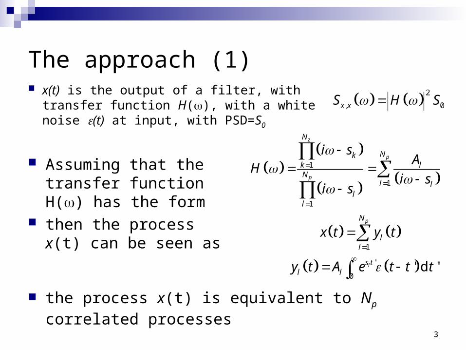
The approach (1) x(t) is the output of a filter, with transfer

function H(), with a white noise (t) at input, with PSD=S0

2

, 0x xS H S

1

1

1

z

p

p

N

Nkk lN

l ll

l

i sA

Hi s

i s

Assuming that the transfer

function H() has the form

then the process x(t) can be seen as

1

pN

ll

x t y t

'

0' d 'ls t

l ly t A e t t t

the process x(t) is equivalent to Np correlated processes

4

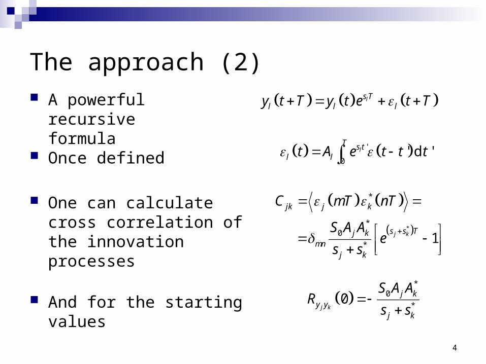
The approach (2)

Once defined

A powerful recursive formula

ls Tl l ly t T y t e t T

'

0' d 'l

T s tl lt A e t t t

One can calculate cross correlation of the innovation processes

*

*

*0

* 1j k

jk j k

s s Tj kmn

j k

C mT nT

S A Ae

s s

*

0

*0

j k

j ky y

j k

S A AR

s s

And for the starting values

5

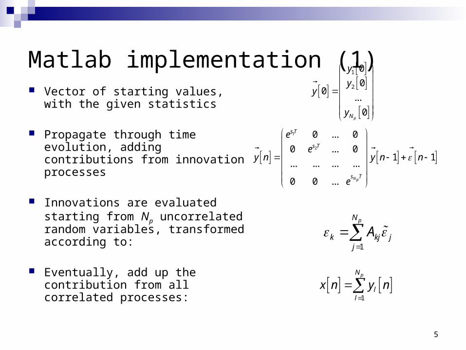
Matlab implementation (1) Vector of starting values, with the

given statistics

Propagate through time evolution, adding contributions from innovation processes

Innovations are evaluated starting from Np uncorrelated random variables, transformed according to:

Eventually, add up the contribution from all correlated processes:

1

2

0

00

...

0pN

y

yy

y

1

2

0 ... 0

0 ... 01 1

... ... ... ...

0 0 ... Np

s T

s T

s T

e

ey n y n n

e

1

pN

ll

x n y n

1

pN

k kj jj

A

6

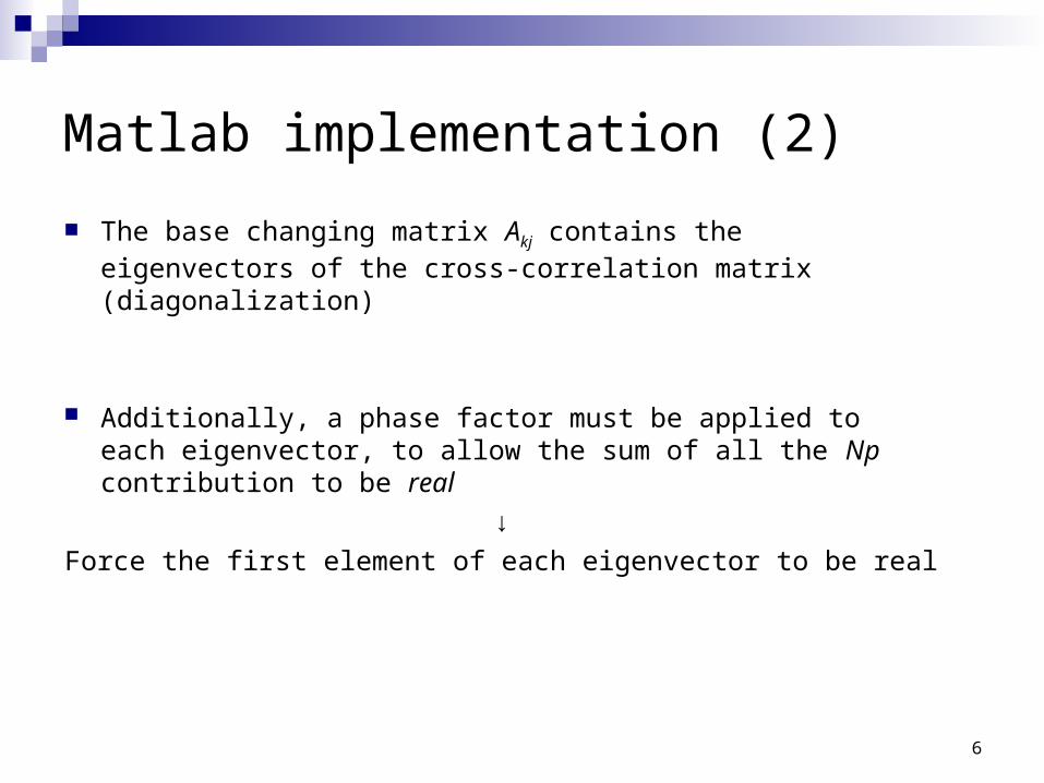
Matlab implementation (2)

The base changing matrix Akj contains the eigenvectors of the cross-correlation matrix (diagonalization)

Additionally, a phase factor must be applied to each eigenvector, to allow the sum of all the Np contribution to be real

↓

Force the first element of each eigenvector to be real

7

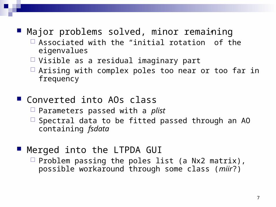
Major problems solved, minor remaining Associated with the “initial rotation” of the eigenvalues Visible as a residual imaginary part Arising with complex poles too near or too far in frequency

Converted into AOs class Parameters passed with a plist Spectral data to be fitted passed through an AO containing

fsdata

Merged into the LTPDA GUI Problem passing the poles list (a Nx2 matrix), possible

workaround through some class (miir?)

8

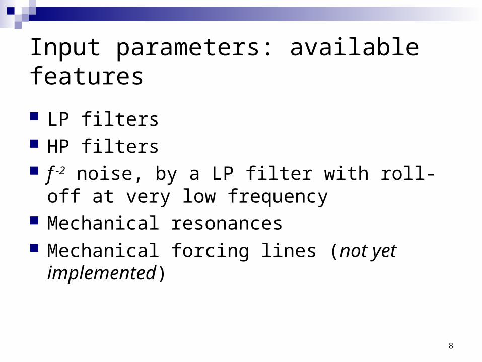
Input parameters: available features

LP filters HP filters f -2 noise, by a LP filter with roll-off at very low

frequency Mechanical resonances Mechanical forcing lines (not yet implemented)

9

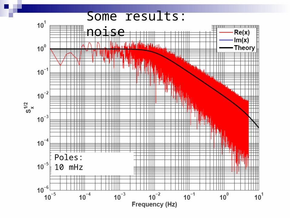
Some results: noise

Poles: 10 mHz

10

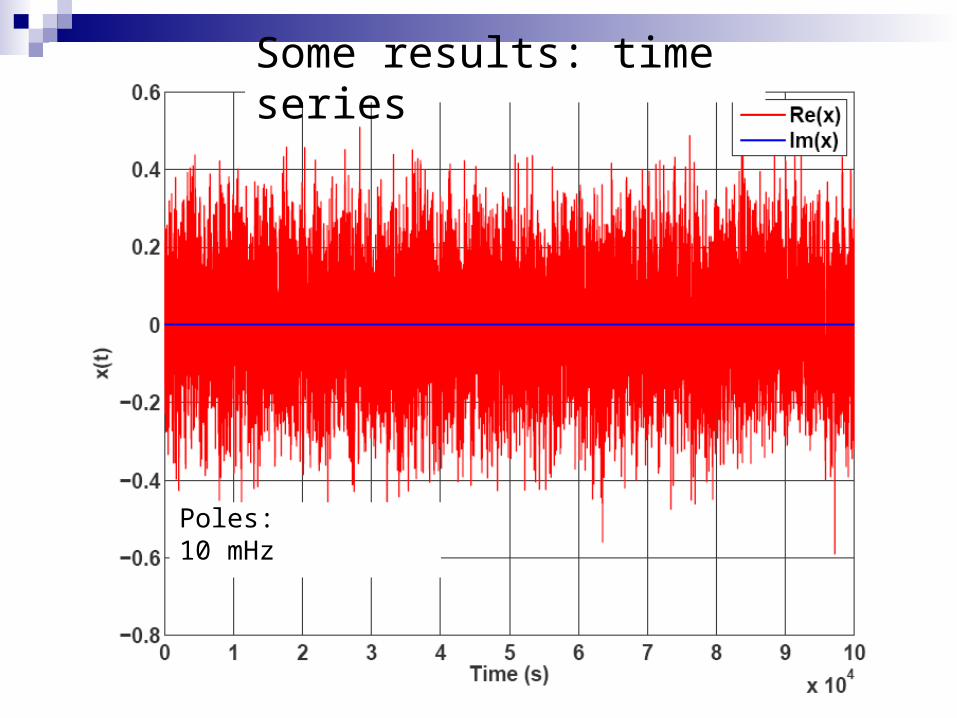
Some results: time series

Poles: 10 mHz

11

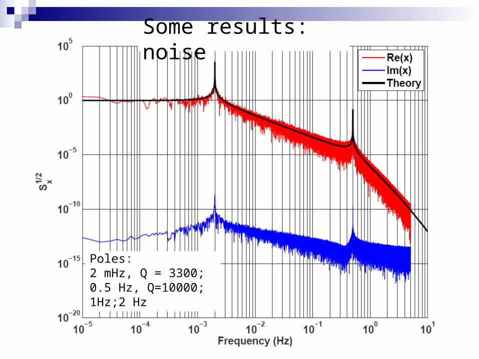
Some results: noise

Poles: 2 mHz, Q = 3300; 0.5 Hz, Q=10000;1Hz;2 Hz

12

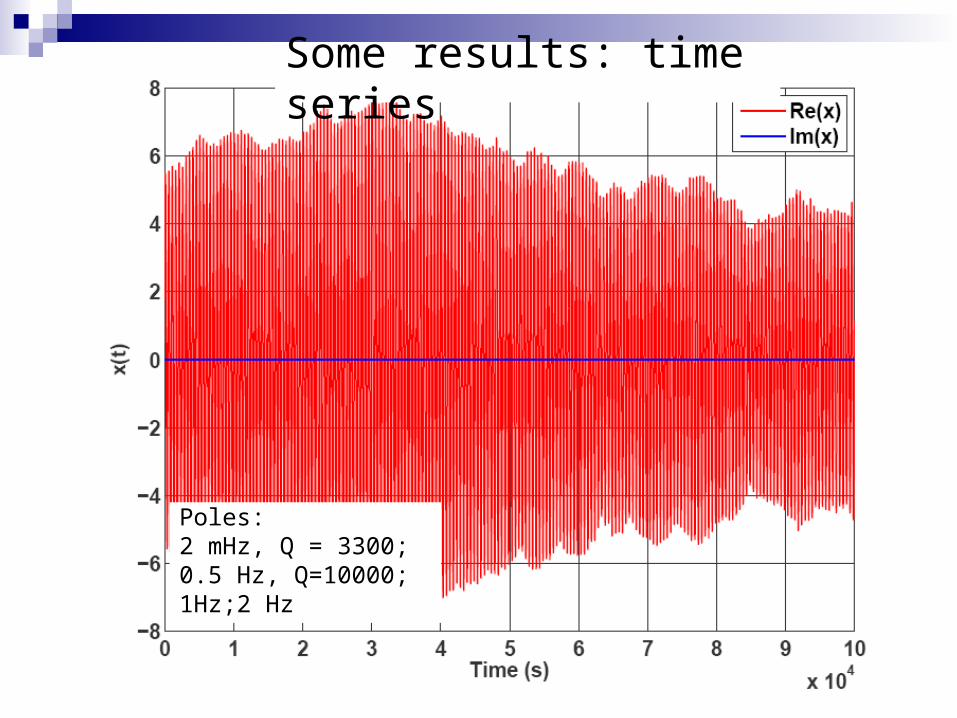
Some results: time series

Poles: 2 mHz, Q = 3300; 0.5 Hz, Q=10000;1Hz;2 Hz

13

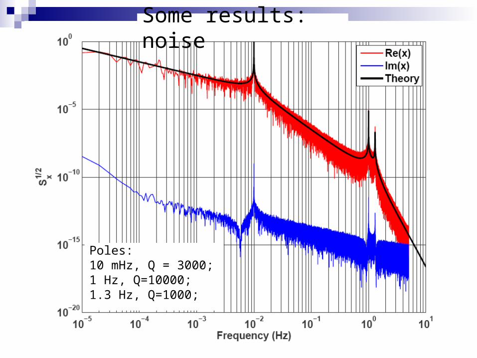
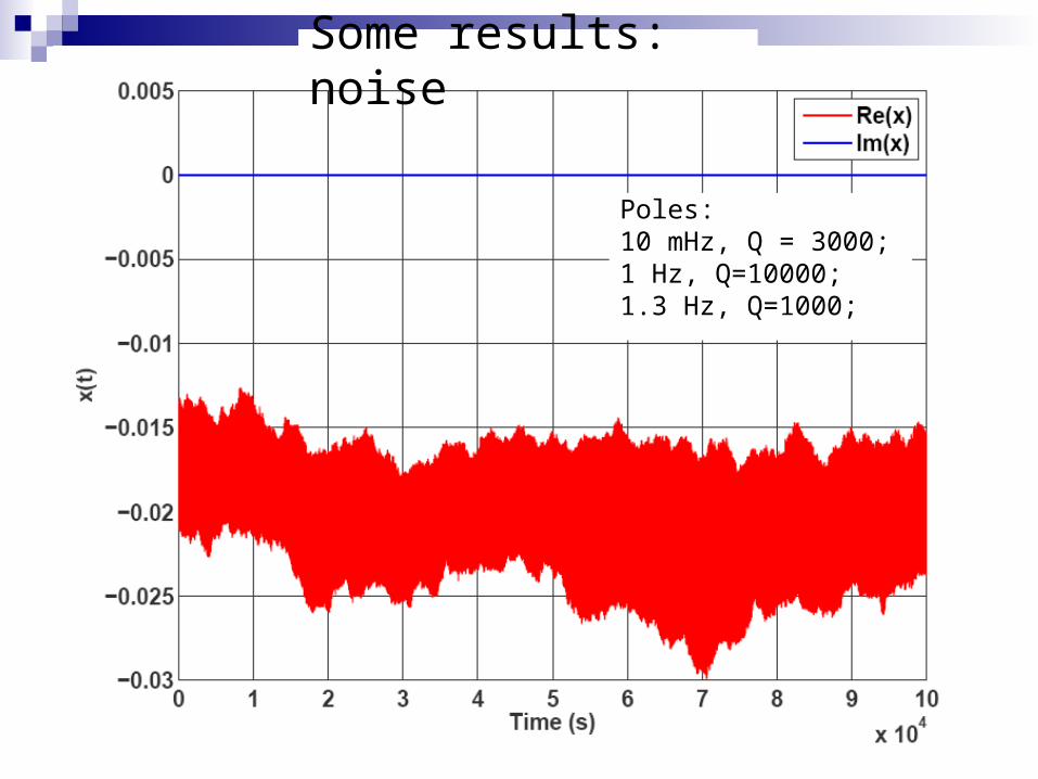
Some results: noise

Poles: 10 mHz, Q = 3000; 1 Hz, Q=10000;1.3 Hz, Q=1000;

14

Some results: noise

Poles: 10 mHz, Q = 3000; 1 Hz, Q=10000;1.3 Hz, Q=1000;

15

What comes next:

Get the fitting features to work Compare with AEI noise generator Use it as the tools for system identification