Using WinBUGS to Cox Model with Changing from the Baseline

Applied Mathematical Sciences, Vol. 5, 2011, no. 45, 2217 - 2240

Using WinBUGS to Cox Model with Changing

from the Baseline Hazard Function

Ayman A. Mostafa and Anis Ben Ghorbal

Department of Mathematics Al-Imam Muhammad Ibn Saud Islamic University

P.O. Box 90950, 11623 Riyadh, Saudi Arabia [email protected]; [email protected]

Abstract

The proportional hazards model (PHM) in the context survival data analysis, take in the famous Cox model as it is also called, was introduced by Cox (1972) in order to estimate the effects of different covariates influencing the times-to-event data. It’s well known that Bayesian analysis has the advantage in dealing with censored data and small sample over frequentist methods. Therefore in this paper we discuss the PHM for right-censored death times from Bayesian perspective, and then compute the Bayesian estimator based on the Markov Chain Monte Carlo (MCMC) method. Survival model can be conveniently inspected with the help of hazard function. A common approach to handling the prior probability for the baseline hazard function in PHM is a Gamma process prior. However, this can lead to biased and misleading results (Spiegelhalter et al., 1996). The Gibbs sampling is proposed to simulate the Markov chain of parameters’ posterior distribution dynamically, which avoids the calculation of complex integrals of the posterior using WinBUGS package. For the problem, we adopt the idea behind the polygonal baseline hazard approach proposed in Beamonte and Bermúdez (2003) to develop the estimation for the survival curves. The proposed methodology is illustrated by re examining two textbook data examples.

Mathematics Subject Classification: 62N99, 62F15, 62M20, 65C05, 65C40, 68N15 Keywords: Proportional hazards model; posterior distributions; Markov chain Monte Carlo; Model comparison (DIC); WinBUGS

1 Introduction The modeling and analysis survival data is one of the oldest fields of

statistics, going back to the beginning of the development of actuarial science and

2218 A. A. Mostafa and A. B. Ghorbal

demography in the 17th century. As the name indicates, survival data deals with life times or, more generally, with waiting times from some initial event at time 0 (like birth, start of treatment or employment in a given job) to some terminal event of interest (like death, relapse or disability pension). Thus the basic data would ideally be independent non-negative random variable T. A major advance in the field of survival analysis took place 1950's. The induction of this new phase is represented by the paper Kaplan and Meier (1958) where they propose their famous estimator of the survival curve. This is one of the most cited papers in the history of statistics with more than 35,000 citations in the ISI Web of knowledge. Their proposal might call a continuous-time version of the old life table. The 1958 Kaplan-Meier paper opened a new area, but also raised a number of questions. How, for instance, does one compare between the diagnostic factors (covariates) from the collected sample. Hence, the more general issue of how to adjust for covariates was first resolved by the introduction of the proportional hazards model (PHM) by David Cox in 1972. This was a major advance, and the more than 25,000 citations that Cox's paper has attracted in the ISI Web of knowledge is a proof of its huge impact (Aalen et al., 2009).

In biomedical applications, especially in clinical trials, important issue arise when studying ”time to event” data that is some individuals are still alive at the end of the study or analysis so the event of interest, namely death, has not occurred. Therefore we have right censored data. In order that the estimates of the suggested survival model give unbiased results there is an important assumption that individuals who are censored are at the same risk of subsequent failure as those who are still alive and uncensored. The risk set at any time point (the individuals still alive and uncensored) should be representative of the entire population alive at the same time. If this is the case, the censoring process is called non-informative. Statistically, if the censoring process is independent of the survival time, then we will automatically have non-informative censoring. Actually, we almost always mean independent censoring by non-informative censoring. The primary goal in analyzing censored survival data is to assess the dependence of survival time on covariates. The secondary goal is the estimation of the underling distribution of survival time.

PHM, which we will concentrate on in this article, is the multiple hazard model or PHM, which has been used extensively since Cox (1972) introduced it in the context of univariate failure time data (if every subject of the study can experience the event at most once, such as death of individual, then the data are called univariate survival data).

In a fully parametric model, the strong assumption is made that the lifetime distribution belongs to a given family of parametric distributions and the regression problem is reduced to estimating the parameters from the data (see e.g., Feigl and Zelen, 1965). However, the fully parametric models are difficult to apply without fore knowledge of the form of the hazard functions which are the very object of the study.

For modeling PHM from classical perspective, Kalbfleisch and Prentice (1980)

Using WinBUGS to Cox model 2219

described in details how Cox (1972, 1975) obtained the partial likelihood approach to estimate the unknown parameters. Kumar and Klefsjö (1994) have introduced an excellent paper in PHM from classical approach. Their paper a detailed review has been presented. From a Bayesian perspective, that model has been the most common. Sinha and Dey (1997) have proposed an excellent paper in this area. In their paper a review of its statistical treatment have been presented. A landmark in the development of Bayesian survival analysis is the 2001 book by Ibrahim, Chen, and Sinha (simply titled ‘Bayesian Survival Analysis’). As far as we know, it is the only book-length treatment on the topic to date. For instance, in their Book (Ch. 3) survey the large recent literature on semi-parametric Bayesian approaches to failure time models. Much of this work focuses on the use of gamma, beta, and Dirichlet processes to model functions across time, i.e., baseline hazards and time-dependent covariate effects. While there is much to commend this work, for the most part it is relatively complex to implement. This may be an impediment to practitioners who wish to use such techniques. On the other hand, the reason why such Bayesian methods had not been widely used in survival analysis until the last few years is because, for such realistic models, the posterior distribution under censoring is extremely difficult to obtain directly. The development of new numerical algorithms, such as Gibbs sampling, which allow obtaining samples from the posterior of interest has motivate the use of Bayesian methods in survival analysis. Fully Bayesian computation of more than one level (multi-level or hierarchical) model are now possible using simulation, techniques. The Gibbs sampler may be one of the best known Markov chain Monte Carlo (MCMC) sampling algorithm in such computational literature. MCMC techniques have become an elegant tool in Bayesian analysis. As mentioned in many papers such as Brooks (1998), the Gibbs sampler is introduced in the context of image processing by Geman and Geman (1984). Although many authors appearing in the papers explain MCMC-based Bayesian analysis as this task would typically require significant scientific programming ability and facility with such random number generators. Fortunately, specialized software for implementing MCMC analyses is now available. Thus, this paper describes the use of freely available software for the analysis of complex statistical models using MCMC techniques, called WinBUGS, in the context of PHM. BUGS (Spiegelhalter, et. al., 1996) is specialized software package for implementing MCMC-based analyses of full probability models in which all unknowns are treated as random variables. The BUGS project began at the Medical Research Council Biostatistics Unit in Cambridge in 1989. Since that time the software has become one of the most popular statistical modeling packages, with, at the time of writing, over 30,000 registered users of WinBUGS worldwide. BUGS has been just one part of the tremendous growth in the application of Bayesian ideas over the last 20 years. Prior to the widespread introduction of simulation-based methods, Bayesian ideas could only be implemented in circumstances in which solutions could be obtained in closed form in so-called conjugate analyses, or by ingenious but restricted application of numerical integration methods. The importance of the software has


been acknowledged in ‘An International Review of U.K. Research in Mathematics’(http://www.cms.ac.uk/irm/irm.pdf). It turns out that WinBUGS can become quite a powerful and flexible tool for Bayesian survival analysis, and only requires a relatively small investment on the part of the user. Once the (applied) user understands the logic of model building with WinBUGS, Bayesian analysis is conducted quite easily and many built-in features can be accessed to produce an in-depth and interactive analysis of PHM. In addition, execution is reasonably fast, even of complicated models with large amounts of data and model extensions can easily be accommodated in a modular fashion. The WinBUGS software (together with a user manual) can be downloaded (the current fee is zero) from the website (http://www.mrc-bsu.cam.ac.uk/bugs/winbugs/contents.shtml). We illustrate the use and flexibility of WinBUGS for Bayesian survival modeling of the Leukemia Data example, which has introduced by Spiegelhalter et al. (1996). In their example, they follow the seminal paper by Kalbfleisch (1978) to describe the gamma process prior for the baseline cumulative hazard function. The objective of the current paper is to propose an alternative approach and describe a Bayesian semi-parametric approach to solve a hierarchical model for PHM. The non-parametric part of the Cox model is supposed to be a non-negative polygonal function. That approach has been used before (see Beamonte and Bermúdez (2003)) but with additive hazard model and they did not do a model comparison with other models such as the use of PHM. Beamonte and Bermúdez wrote a long portable FORTRAN code which consists of several hundred of lines to code their contribution. Using WinBUGS, we will illustrate, it is easily to reduce to literally one or two dozen lines of code in WinBUGS and it straightforward to compare the models using the deviance information criterion (DIC) tool, which is available in the currently WinBUGS 1.4.3 (Spiegelhalter et al. (2003)). The structure of this paper is as follows.

Section 2, first we demonstrate the importance of incorporating covariates into the distribution in prediction. Second, we introduce a Bayesian MCMC approach for Cox Model as a review and describe the polygonal baseline hazard using ideas from Beamonte and Bermúdez (2003). Section 3 shows how the method can be adapted using WinBUGS software and illustrate method by two examples based on real data. The paper concludes with a discussion.

2 A Bayesian MCMC approach for PHM

2.1 Application of martingales in the Cox model

The analysis of counting process data, including survival data, is usually based on the modeling of the intensity. Let the random variable T denote the survival time of an individual, then the survival curve is given by ( ) ( )S t P T t= > . It is useful when considering survival data to partition time into many small


intervals, say, with interval length equal to tΔ , where tΔ is small. Assuming that T is absolutely continuous (i.e., has a probability density), one looks at those who have survived up to some time ,t and considers the calculating the probability of an event happening over some finite time interval[ , )t t t+ Δ . The baseline hazard rate 0( ),tλ common to all subjects, is defined as the following limit:

00 lim( )( )

t

P t T t ttt

λΔ →

≤ < + Δ=

Δ (2.1)

0 ( )tλ in (2.1) can be interpreted as the instantaneous death (or event) rate of an individual, provided that this person survived until time t. In particular,

0 ( )t tλ Δ is the approximate probability of failure in[ , )t t t+Δ , given survival up to time t. While it is simple to estimate the survival curve, it is more difficult to estimate the hazard rate as an arbitrary function of time. What, however, is quite easy is to estimate the baseline cumulative hazard rate defined as

0 00

( ) ( ) t

t s dsλΛ = ∫ (2.2)

A non-parametric estimator of 0( )tΛ was first suggested by Nelson (1969) as a graphical tool to obtain engineering information on the form of the survival distribution in reliability studies. The same estimator was independently suggested by Altshuler (1970) and by Aalen (1972). With the development of clinical trials in the 1950’s and 1960’s the need to analyze censored survival data dramatically increased, and a major breakthrough in this direction was the Cox proportional hazards model published in 1972 (Cox, 1972). Now, regression analysis of survival data was possible. Specifically, the Cox model describes the hazard function (also called the risk function or intensity function) for a subject i with covariates 1( , ..., )i i ipZ Z Z= as

[ ] 0( | ) ( | 0) exp ( )exp( )t Z t Z Z t Zλ λ β λ β′= = = ′ (2.3)

This is a product of the unknown baseline hazard rate 0 ( )tλ (the nonparametric part) and the exponential function of the unknown regression coefficient,

j ijjZ Zβ β′ =∑ (the parametric part). Typically; both β and Z are assumed

to be constant over time t .

The parameters of the model are the p-dimensional regression parameter β and the nonparametric baseline hazard rate 0 ( )tλ that is assumed to be locally integrable:


max

00

( )T

t dtλ < ∞∫ with maxT denoting the time point where the study is stopped. The

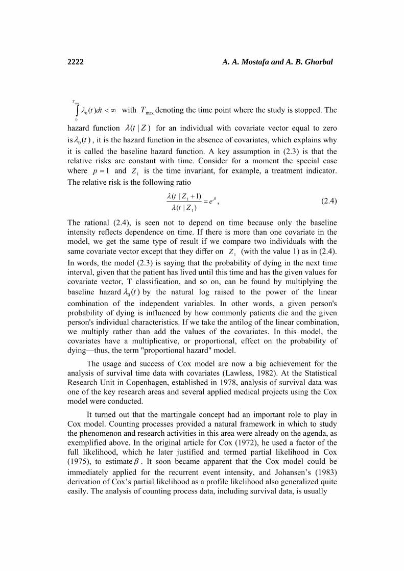
hazard function ( | )t Zλ for an individual with covariate vector equal to zero is 0 ( )tλ , it is the hazard function in the absence of covariates, which explains why it is called the baseline hazard function. A key assumption in (2.3) is that the relative risks are constant with time. Consider for a moment the special case where 1p = and 1Z is the time invariant, for example, a treatment indicator. The relative risk is the following ratio

1

1

( | 1)( | )

,t Ze

t Zβλ

λ+

= (2.4)

The rational (2.4), is seen not to depend on time because only the baseline intensity reflects dependence on time. If there is more than one covariate in the model, we get the same type of result if we compare two individuals with the same covariate vector except that they differ on 1Z (with the value 1) as in (2.4). In words, the model (2.3) is saying that the probability of dying in the next time interval, given that the patient has lived until this time and has the given values for covariate vector, T classification, and so on, can be found by multiplying the baseline hazard 0 ( )tλ by the natural log raised to the power of the linear combination of the independent variables. In other words, a given person's probability of dying is influenced by how commonly patients die and the given person's individual characteristics. If we take the antilog of the linear combination, we multiply rather than add the values of the covariates. In this model, the covariates have a multiplicative, or proportional, effect on the probability of dying—thus, the term "proportional hazard" model.

The usage and success of Cox model are now a big achievement for the analysis of survival time data with covariates (Lawless, 1982). At the Statistical Research Unit in Copenhagen, established in 1978, analysis of survival data was one of the key research areas and several applied medical projects using the Cox model were conducted.

It turned out that the martingale concept had an important role to play in Cox model. Counting processes provided a natural framework in which to study the phenomenon and research activities in this area were already on the agenda, as exemplified above. In the original article for Cox (1972), he used a factor of the full likelihood, which he later justified and termed partial likelihood in Cox (1975), to estimate β . It soon became apparent that the Cox model could be immediately applied for the recurrent event intensity, and Johansen’s (1983) derivation of Cox’s partial likelihood as a profile likelihood also generalized quite easily. The analysis of counting process data, including survival data, is usually


based on the modeling of the intensity.

Andersen and Gill (1982) extended (2.3) to the counting process framework and gave elegant martingale proofs for the asymptotic properties of the associated estimators in the models try to fit models for survival data. Others that have contributed to establishing asymptotic results for the model are Tsiatis (1981) Næs (1982). If we have n subjects under investigations, for subject i ,

1, 2,..., ,i n= ( )iI t is the intensity process for a counting process given covariate vector 1( ,..., )i i ipZ Z Z= , and ( )iY t is the at risk indicator, i.e., the set of subjects still at risk at the time, iT , of failure for subject i (i.e., alive and

uncensored at time point just before time t ), furthermore, we observe process ( ),iN t to count the number of failures which occurred in the interval [0, ]t . That

process is constant and equal to zero between failures and jumps one unit at each failure time. Since the stochastic process { }( ), 0iN t t ≥ is counting process, then it is satisfies the following conditions:

i. ( ) 0,iN t ≥ ii. ( )iN t takes integer values,

iii. If , ( ) ( )i is t N t N s< − represents the number of failures that occurred in the time interval [ , ].s t

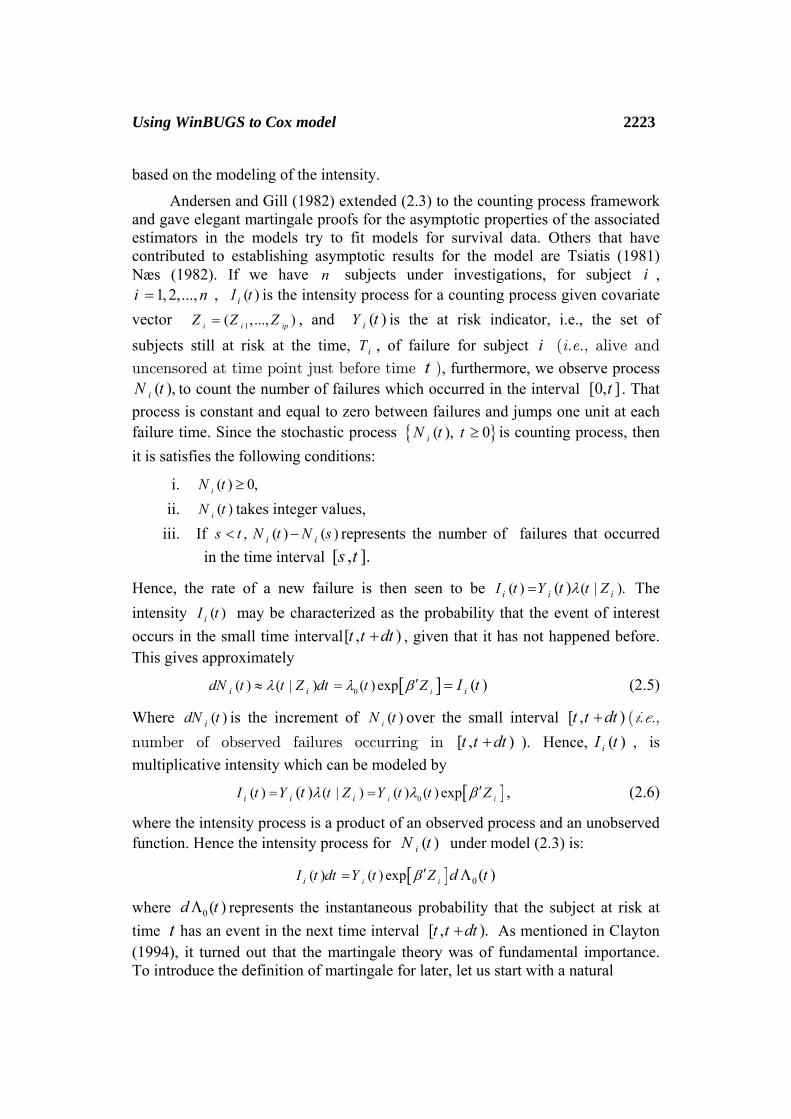
Hence, the rate of a new failure is then seen to be ( ) ( | ).( )i i iI t Y t Zt λ= The intensity ( )iI t may be characterized as the probability that the event of interest occurs in the small time interval[ , )t t dt+ , given that it has not happened before. This gives approximately

[ ]0( ) ( | ) ( ) exp ( )ii i idN t t Z dt t Z I tλ λ β ′≈ = = (2.5)

Where ( )idN t is the increment of ( )iN t over the small interval [ , )t t dt+ (i.e.,

number of observed failures occurring in [ , )t t dt+ ). Hence, ( )iI t , is multiplicative intensity which can be modeled by

[ ]0( ) ( | ) ( ) ( ) exp( ) i ii i iI t Y t Z Y t t Zt λ λ β ′= = , (2.6)

where the intensity process is a product of an observed process and an unobserved function. Hence the intensity process for ( )iN t under model (2.3) is:

[ ] 0( ) ( ) exp ( )i iiI t dt Y t Z d tβ ′= Λ

where 0 ( )d tΛ represents the instantaneous probability that the subject at risk at time t has an event in the next time interval [ , ).t t dt+ As mentioned in Clayton (1994), it turned out that the martingale theory was of fundamental importance. To introduce the definition of martingale for later, let us start with a natural


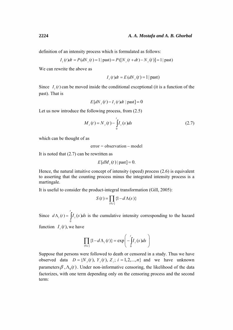
definition of an intensity process which is formulated as follows:

( ) ( ( ) 1| past) ([ ( ) 1| past)( )]i ii iI t dt P dN t P N t dt N t= = = + − =

We can rewrite the above as

( ) ( ( ) 1| past)i iI t dt E dN t= =

Since ( )iI t can be moved inside the conditional exceptional (it is a function of the past). That is

[ ( ) | past( ) ] 0i iE dN I t dtt − =

Let us now introduce the following process, from (2.5)

0

( ) ( ) ( )t

i i iM t N t I s ds= − ∫ (2.7)

which can be thought of as error = observation model−

It is noted that (2.7) can be rewritten as

[ | past( ) ] 0.iE dM t =

Hence, the natural intuitive concept of intensity (speed) process (2.6) is equivalent to asserting that the counting process minus the integrated intensity process is a martingale.

It is useful to consider the product-integral transformation (Gill, 2005):

(0, ]

( ) {1 ( )}t

S t d s= − Λ∏

Since 0

( ) ( )t

i id t I s dsΛ = ∫ is the cumulative intensity corresponding to the hazard

function ( ),iI t we have

(0, ] 0

{1 ( )} exp ( )t

i it

d t I s ds⎛ ⎞

− Λ = −⎜ ⎟⎝ ⎠

∏ ∫

Suppose that persons were followed to death or censored in a study. Thus we have observed data { ( ), ( ), ; 1,2,..., }ii iD Y ZN t t i n= = and we have unknown parametersβ , 0 ( )tΛ . Under non-informative censoring, the likelihood of the data factorizes, with one term depending only on the censoring process and the second term:


[ ] ( )

00

( )) exp( | , ( ) ( ) i

i

dN ti i i

tt

tL D I t dt I tβ≥≥

Λ =⎛ ⎞−⎜ ⎟⎝ ⎠

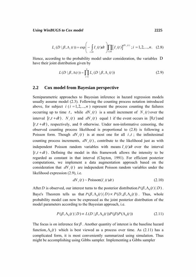
∏∫ ; 1,2,..., .i n= (2.8)

Hence, according to the probability model under consideration, the variables D have their joint distribution given by

1

( ))( | , ( | , ( ))n

i ii

tL D L D tβ β=

Λ = Λ∏ (2.9)

2.2 Cox model from Bayesian perspective

Semiparametric approaches to Bayesian inference in hazard regression models usually assume model (2.3). Following the counting process notation introduced above, for subject i ( 1,2,...,i n= ) represent the process counting the failures occurring up to time ,t while ( )idN t is a small increment of ( )iN t over the interval [ , )t t dt+ . ( )iN t and ( )idN t equal 1 if the event occurs in [0, )t and [ , )t t dt+ , respectively, and 0 otherwise. Under non-informative censoring, the observed counting process likelihood is proportional to (2.8) is following a Poisson form. Though ( )idN t is at most one for all ,i t ; the infinitesimal counting process increments, ( )idN t , contribute to the likelihood just as with independent Poisson random variables with means ( )iI t dt over the interval [ , )t t dt+ . Defining the model in this framework allows the intensity to be regarded as constant in that interval (Clayton, 1991). For efficient posterior computations, we implement a data augmentation approach based on the consideration that ( )idN t are independent Poisson random variables under the likelihood expression (2.9), i.e.

( ) )( ) ~ Poisson( iid I t dtN t (2.10)

After D is observed, our interest turns to the posterior distribution 0( , ( ) | )P t Dβ Λ . Baye's Theorem tells us that 0 0( , ( ) | ) ( , , ( ))P t D P D tβ βΛ ∝ Λ . Thus, whole probability model can now be expressed as the joint posterior distribution of the model parameters according to the Bayesian approach, i.e.

0 0 0( , ( ) | ) ( | , ( )) ( ) ( ( ))P t D L D t P P tβ β βΛ ∝ Λ Λ (2.11)

The focus is on inference forβ . Another quantity of interest is the baseline hazard function, 0( )tΛ which is best viewed as a process over time. As (2.11) has a complicated form, it is most conveniently summarized using simulation. Thus might be accomplishing using Gibbs sampler. Implementing a Gibbs sampler

2226 A. A. Mostafa and A. B. Ghorbal coded from scratch would require us to identify and then construct an effective simulation method for each of the two related full conditional posterior distributions, namely 0| )( , ( )P D tβ Λ , 0 | )( ( ) ,P t D βΛ . These are exactly the same tasks the WinBUGS software obviates, as it performs these steps internally and automatically. Various Bayesian formulations of the model (2.11) differ mainly in the nonparametric specification of 0 ( )tΛ . 2.3 Modeling the baseline hazard using the polygonal function

Using ideas from Beamonte and Bermúdez (2003), again Consider the multiplicative intensity model in (2.3):

[ ]0( ) ( ) ( ) expi iiI t Y t t Zλ β′= The non-parametric part of the model, 0 ( )tλ , is supposed to be a non-negative polygonal function with the vertices located at times

max0 1 10 ... T Ta a a a += < < < < , where the polygonal takes the values

max max0 1 2 10 ... T Tτ τ τ τ τ += < < < < < ,

respectively and becomes constant after time max 1Ta + , can be written as:

max

11 max

10

1 max

( )( ) if a t a , 1,...,

( ) if t T 1

j j jj j j

j j

T

t aj T

a at

τ ττ

λτ

++

+

+

− −⎧+ ≤ ≤ =⎪ −= ⎨

⎪ ≥ +⎩

(2.12)

The (2.12) is formulated in Display 1 through line 18. The advantage from using (2.12), instead of the usual step function, that ( )iI t will be continuous. The gamma process prior of Kalbfleisch (1978) assumes independent cumulative hazards increment. This is unrealistic in most applied settings, and does not allow for borrowing of strength between adjacent intervals. The idea of smoothing by treating the prior for the vector τ , which can be specified as an auto-correlated first order process, following Gamerman (1991) who proposed it in a related context. Then

1 exp( )j j jeτ τ+ = , max1,...,j T= (2.13) The (2.13) is formulated in Display 1 through line 16. Where ( )max1 T,...,e e are supposed to be independent, logNormal distributed with

mean zero and variance 2eσ , and

1 1 τ τ~ Gamma(τ |a ,b )τ (2.14) The (2.14) is formulated in Display 1 through line 20, with taking 0.01a bτ τ= = , This choice implies that the a prior mean equals 1 and the variance equals 500 for the parameter 1τ

2e e~ Gamma(tau.e|a ,b )eσ ; where


2tau.e 1/ eσ= (2.15) The (2.15) is formulated in Display 1 through line 22, with taking 0.001e ea b= = . Parameter estimates and the 95% credible intervals (CI) can be obtained from the MCMC samples. Some caution should be exercised because the choice of hyperparameters may affect the final parameter estimates. 3 Examples for simulation analyses

The following sections illustrate the power of WinBUGS to produce useful summary statistics and graphical representations of the posterior distribution with two example datasets. We also show how changes to the model specification can be implemented quite easily. In addition, we discuss how to improve the results of survival models. 3.1 Leukemia data (Comparing treatments for leukemia remission)

To illustrate how the method for multiplicative-polygonal hazards works,

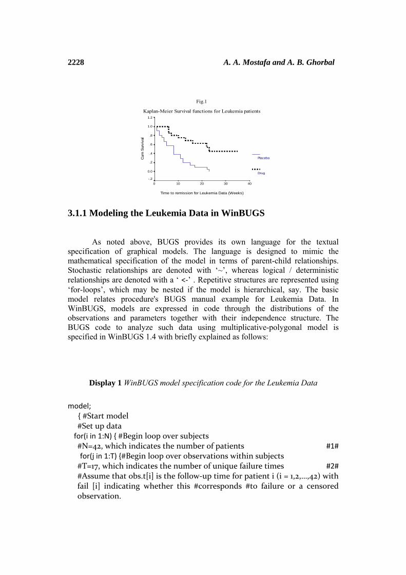
we apply it to the first simulated example analyses. The data are taken from Kalbfleisch and Prentice, 1980, PP. 205–206, for comparing the remission times (in weeks) for patients subjected to different treatments. The patients were receiving a new drug (6-MP) with control patient, (placebo effect drug). The total of patients is 42. Among the 42 observed remission times, 12 times were censored, there are 17 distinct death times were observed, and the last remission time was (censored). Group membership is the only covariate of interest and is specified by Z , we fit the model with iZ = 0.5 , if the ith patient belongs to treatment placebo and 0.5− otherwise. We provide the entire program in the Display 1. Equations and describes the core components (likelihood and the main assumptions of the model) and is specified in WinBUGS and explained in the following subsection. The Kaplan and Meier estimates for the survival functions of both treatment groups (Figure 1) suggest that a proportional hazard model is appropriate. In our final study, we used vertices at time points given by the components of the following vector as follows:

a=c(2,4,6,8,10,12,14,16,18,20,22,24,26,28,30,32,34,36). This seemed to be suitable choice among other experimented portions of time and had not a better fit with more than seventeen disjoint intervals. It was found from both frequentist and Bayesian previous analysis that, a proportional hazard model is appropriate for these data (see, The Kaplan and Meier estimates for the survival functions of both treatments in Figure 1).


Fig.1

Kaplan-Meier Survival functions for Leukemia patients

Time to remission for Leukemia Data (Weeks)

403020100

Cum

Sur

viva

l

1.2

1.0

.8

.6

.4

.2

0.0

-.2

Placebo

Drug

3.1.1 Modeling the Leukemia Data in WinBUGS

As noted above, BUGS provides its own language for the textual specification of graphical models. The language is designed to mimic the mathematical specification of the model in terms of parent-child relationships. Stochastic relationships are denoted with ‘~’, whereas logical / deterministic relationships are denoted with a ‘ <‐’ . Repetitive structures are represented using ‘for-loops’, which may be nested if the model is hierarchical, say. The basic model relates procedure's BUGS manual example for Leukemia Data. In WinBUGS, models are expressed in code through the distributions of the observations and parameters together with their independence structure. The BUGS code to analyze such data using multiplicative-polygonal model is specified in WinBUGS 1.4 with briefly explained as follows:

model; { #Start model #Set up data for(i in 1:N) { #Begin loop over subjects #N=42, which indicates the number of patients #1# for(j in 1:T) {#Begin loop over observations within subjects #T=17, which indicates the number of unique failure times #2# #Assume that obs.t[i] is the follow‐up time for patient i (i = 1,2,…,42) with fail [i] indicating whether this #corresponds #to failure or a censored observation.

Display 1 WinBUGS model specification code for the Leukemia Data

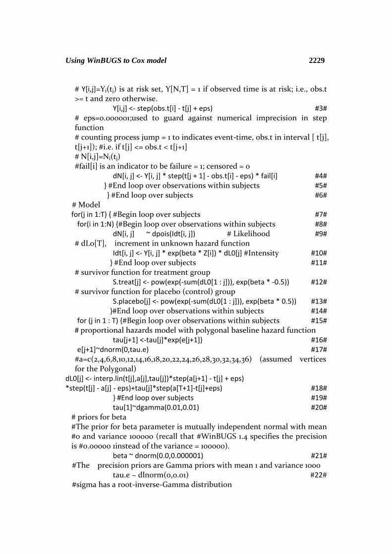
Using WinBUGS to Cox model 2229 # Y[i,j]=Yi(tj) is at risk set, Y[N,T] = 1 if observed time is at risk; i.e., obs.t >= t and zero otherwise.

Y[i,j] <‐ step(obs.t[i] ‐ t[j] + eps) #3# # eps=0.000001;used to guard against numerical imprecision in step function # counting process jump = 1 to indicates event‐time, obs.t in interval [ t[j], t[j+1]); #i.e. if t[j] <= obs.t < t[j+1] # N[i,j]=Ni(tj) #fail[i] is an indicator to be failure = 1; censored = 0

dN[i, j] <‐ Y[i, j] * step(t[j + 1] ‐ obs.t[i] ‐ eps) * fail[i] #4# } #End loop over observations within subjects #5# } #End loop over subjects #6#

# Model for(j in 1:T) { #Begin loop over subjects #7# for(i in 1:N) {#Begin loop over observations within subjects #8#

dN[i, j] ~ dpois(Idt[i, j]) # Likelihood #9# # dL0[T], increment in unknown hazard function

Idt[i, j] <‐ Y[i, j] * exp(beta * Z[i]) * dL0[j] #Intensity #10# } #End loop over subjects #11#

# survivor function for treatment group S.treat[j] <‐ pow(exp(‐sum(dL0[1 : j])), exp(beta * ‐0.5)) #12#

# survivor function for placebo (control) group S.placebo[j] <‐ pow(exp(‐sum(dL0[1 : j])), exp(beta * 0.5)) #13# }#End loop over observations within subjects #14#

for (j in 1 : T) {#Begin loop over observations within subjects #15# # proportional hazards model with polygonal baseline hazard function

tau[j+1] <‐tau[j]*exp(e[j+1]) #16# e[j+1]~dnorm(0,tau.e) #17# #a=c(2,4,6,8,10,12,14,16,18,20,22,24,26,28,30,32,34,36) (assumed vertices for the Polygonal)

dL0[j] <‐ interp.lin(t[j],a[j],tau[j])*step(a[j+1] ‐ t[j] + eps) *step(t[j] ‐ a[j] ‐ eps)+tau[j]*step(a[T+1]‐t[j]+eps) #18#

} #End loop over subjects #19# tau[1]~dgamma(0.01,0.01) #20#

# priors for beta #The prior for beta parameter is mutually independent normal with mean #0 and variance 100000 (recall that #WinBUGS 1.4 specifies the precision is #0.00000 1instead of the variance = 100000).

beta ~ dnorm(0.0,0.000001) #21# #The precision priors are Gamma priors with mean 1 and variance 1000

tau.e ~ dlnorm(0,0.01) #22# #sigma has a root‐inverse‐Gamma distribution


sigma <‐ 1 / sqrt(tau.e) #23# }#End model #24#

Once the model code has been loaded, the data must be specified in a special format. Finally, initial values for the variables being estimated need to be specified. Once the model, data and initial values have been entered, WinBUGS creates compiled code to perform an MCMC algorithm for sampling from the posterior distribution. There are several sampling options including multiple chains to aid convergence diagnosis and thinning of the chain to reduce dependence between successive simulated values.

3.1.2 An analysis of Bayesian modeling process: Leukemia Data

Here we use the model in Section 2. The chain was run with a burn-in of 1,000 iterations with 10,000 retained draws and a thinning to every 100th draw. Convergence was achieved for all parameters based on the rules by Gelman and Rubin (1992). The parameter estimates are not sensitive to the choice of hyperparameters and initial values. Graphical representations of the posterior distribution can indicate problems with the performance of the MCMC algorithm. WinBUGS has a number of tools for reporting the posterior distribution. A simple summary (Table 1) can be generated showing posterior mean, median and standard deviation with a 95% posterior credible interval. Parameter names are related in an obvious way to the model in Sec. 2. A fuller picture of the posterior distribution can be provided using the density option in the Sample Monitor Tool which draws a kernel density estimate of the posterior distribution of any chosen parameter, as in Figure 1. Often, the quantities of primary interest in survival data analysis are the survival curves. There are various other options for displaying the posterior distribution. For example the Compare ... menu item brings up the Comparison Tool that draws model fit for the two groups of patients, which can be plotted as in Figure 2. Table 1 WinBUGS output for the leukemia data: posterior statistics

Node Mean SD MC error 2.5 % Median 97.5 % Start sample

beta 1.539 0.4073 0.005128 0.7682 1.532 2.367 1001 10000

sigma 0.06549 0.1107 0.007736 0.02464 0.00009 0.01761 1001 10000

Here the relative risk of the placebo group compared to the 6MP-group is exp(1.539) = 4.66. WinBUGS automatically implements the DIC (Spiegelhalter et al., 2003) model comparison criterion. This is a portable information criterion quantity that trades off goodness-of-fit against a model complexity penalty. In hierarchical models, deciding the model complexity may be difficult and the


method estimates the ‘‘effective number of parameter’’, denoted here by DP . D is the posterior mean of the deviance (–2 × log likelihood) and D̂ is a plug-in estimate of the latter based on the posterior mean of the parameters. The DIC is computed as DIC = D + DP = D̂ + 2 DP . Lower values of the criterion indicate better fitting models. Table 3 records the values computed, in the format given by WinBUGS. For our purposes here, we will focus only on the DIC value. The method was designed to be easy to implement using a sample from the posterior distribution and the interested reader is directed to Spiegelhalter et al. (2002) for a lively discussion of its merits and its relation to the more usual Bayes factor.

Table 2 WinBUGS output for the leukemia data: DIC with Polygonal Baseline Hazard

D D̂ DIC DP

dN 180.039 177.614 182.464 2.425

total 180.039 177.614 182.464 2.425 In the most popular versions of BUGS (Spiegelhalter , et al. (1996)), the authors described the Cox model based on above data and analysis. When comparing the DIC values for Table 2 (depends on their assumptions) and Table 4 (depends on our assumptions); we find that the prior belief for the Polygonal hazard is preferred for the baseline hazard function in Cox model. Table 3 WinBUGS output for the leukemia data: posterior statistics if the Gamma process is used as a prior belief for the baseline hazard

Node Mean SD MC error 2.5 % Median 97.5 % Start sample

beta 1.555 0.4104 0.006293 0.7658 1.551 2.391 1001 10000

Table 4 WinBUGS output for the leukemia data: DIC with Gamma process Baseline Hazards for Leukemia Data

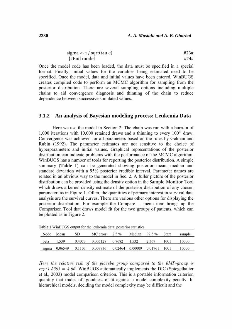
After generating MCMC, Figure 2 shows the evolution of that final sample, using the values for the coefficient of the covariate the two treatment groups, and the Monte Carlo estimate of its marginal distribution. All the hypermeters of the model showed an acceptable convergence to the stationary distribution both with graphical tests, like the one in Figure 2, and with statistical tests which are available in WinBUGS tools software.

D D̂ DIC DP

dN 212.7 192.9 232.6 19.83

total 212.7 192.9 232.6 19.83


Fig 2. WinBUGS output associated to the coefficient of the covariate; group for treatment, on the left, and its estimated posterior density

beta

iteration1001 2500 5000 7500 10000

-1.0 0.0 1.0 2.0 3.0 4.0

beta sample: 10000

-1.0 0.0 1.0 2.0 3.0

0.0 0.25 0.5

0.75 1.0

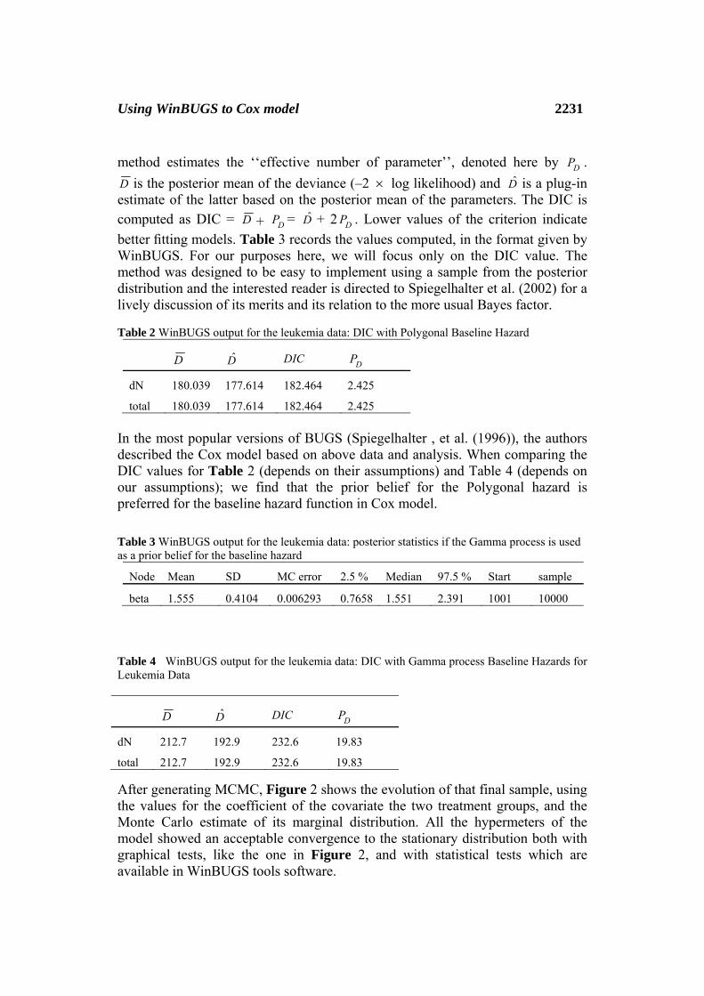
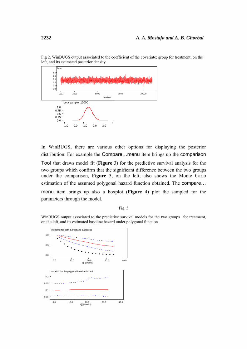
In WinBUGS, there are various other options for displaying the posterior distribution. For example the Compare…menu item brings up the comparison Tool that draws model fit (Figure 3) for the predictive survival analysis for the two groups which confirm that the significant difference between the two groups under the comparison, Figure 3, on the left, also shows the Monte Carlo estimation of the assumed polygonal hazard function obtained. The compare… menu item brings up also a boxplot (Figure 4) plot the sampled for the parameters through the model.

Fig. 3

WinBUGS output associated to the predictive survival models for the two groups for treatment, on the left, and its estimated baseline hazard under polygonal function

model fit for both S.treat and S.placebo

t[j] (Weeks) 0.0 10.0 20.0 30.0 40.0

0.0

0.5

1.0

model fit for the polygonal baseline hazard

t[j] (Weeks) 0.0 10.0 20.0 30.0 40.0

0.05

0.1

0.15

0.2


Fig 4. WinBUGS output associated to the box plot for tau in Display 1

[1][2]

[3][4]

[5][6]

[7][8][9][10]

[11][12]

[13][14][15]

[16][17]

[18]

box plot: tau [1:18]

0.0 0.2 0.4 0.6 0.8

3.2. Larynx Cancer Data (Male laryngeal cancer patients)

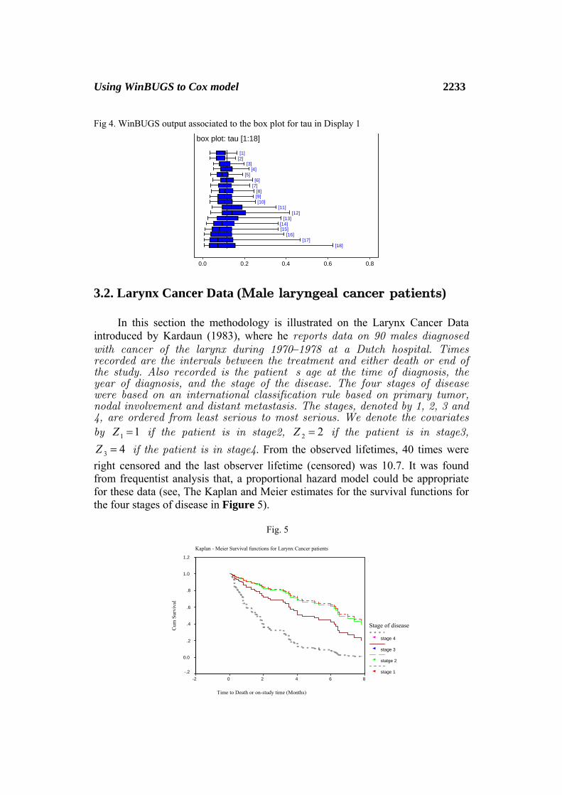
In this section the methodology is illustrated on the Larynx Cancer Data introduced by Kardaun (1983), where he reports data on 90 males diagnosed with cancer of the larynx during 1970–1978 at a Dutch hospital. Times recorded are the intervals between the treatment and either death or end of the study. Also recorded is the patient�s age at the time of diagnosis, the year of diagnosis, and the stage of the disease. The four stages of disease were based on an international classification rule based on primary tumor, nodal involvement and distant metastasis. The stages, denoted by 1, 2, 3 and 4, are ordered from least serious to most serious. We denote the covariates

by 1 1Z = if the patient is in stage2, 2 2Z = if the patient is in stage3,

3 4Z = if the patient is in stage4. From the observed lifetimes, 40 times were right censored and the last observer lifetime (censored) was 10.7. It was found from frequentist analysis that, a proportional hazard model could be appropriate for these data (see, The Kaplan and Meier estimates for the survival functions for the four stages of disease in Figure 5).

Fig. 5

Kaplan - Meier Survival functions for Larynx Cancer patients

Time to Death or on-study time (Months)

86420-2

Cum

Sur

viva

l

1.2

1.0

.8

.6

.4

.2

0.0

-.2

Stage of disease

stage 4

stage 3

statge 2

stage 1

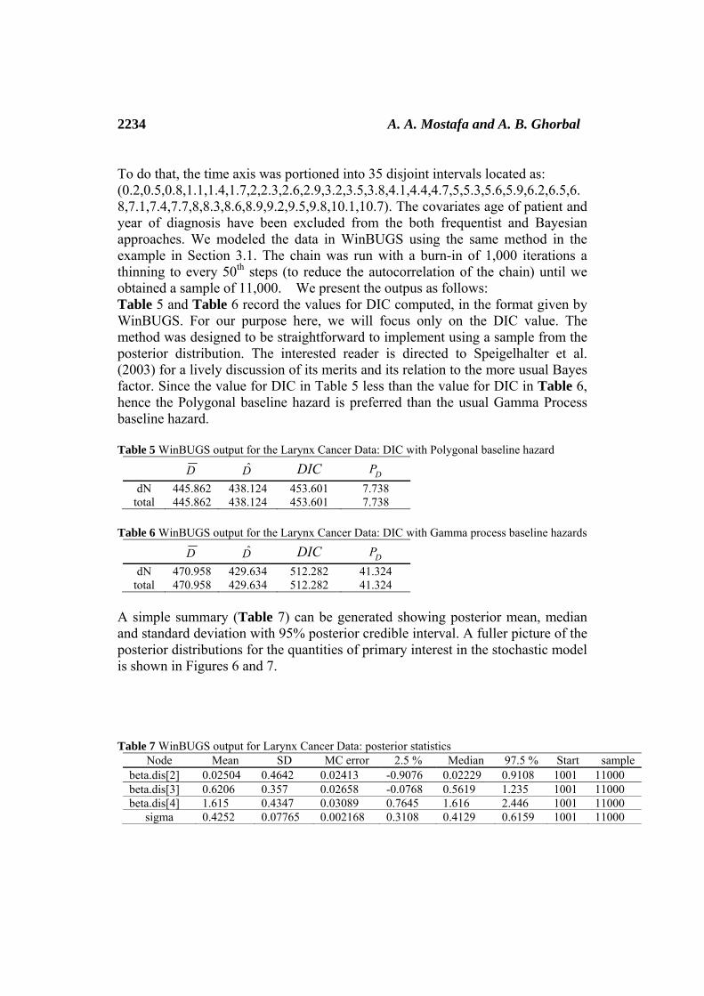
2234 A. A. Mostafa and A. B. Ghorbal To do that, the time axis was portioned into 35 disjoint intervals located as: (0.2,0.5,0.8,1.1,1.4,1.7,2,2.3,2.6,2.9,3.2,3.5,3.8,4.1,4.4,4.7,5,5.3,5.6,5.9,6.2,6.5,6.8,7.1,7.4,7.7,8,8.3,8.6,8.9,9.2,9.5,9.8,10.1,10.7). The covariates age of patient and year of diagnosis have been excluded from the both frequentist and Bayesian approaches. We modeled the data in WinBUGS using the same method in the example in Section 3.1. The chain was run with a burn-in of 1,000 iterations a thinning to every 50th steps (to reduce the autocorrelation of the chain) until we obtained a sample of 11,000. We present the outpus as follows: Table 5 and Table 6 record the values for DIC computed, in the format given by WinBUGS. For our purpose here, we will focus only on the DIC value. The method was designed to be straightforward to implement using a sample from the posterior distribution. The interested reader is directed to Speigelhalter et al. (2003) for a lively discussion of its merits and its relation to the more usual Bayes factor. Since the value for DIC in Table 5 less than the value for DIC in Table 6, hence the Polygonal baseline hazard is preferred than the usual Gamma Process baseline hazard. Table 5 WinBUGS output for the Larynx Cancer Data: DIC with Polygonal baseline hazard

D D̂ DIC DP dN 445.862 438.124 453.601 7.738

total 445.862 438.124 453.601 7.738 Table 6 WinBUGS output for the Larynx Cancer Data: DIC with Gamma process baseline hazards

D D̂ DIC DP dN 470.958 429.634 512.282 41.324

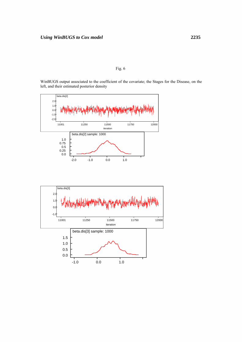
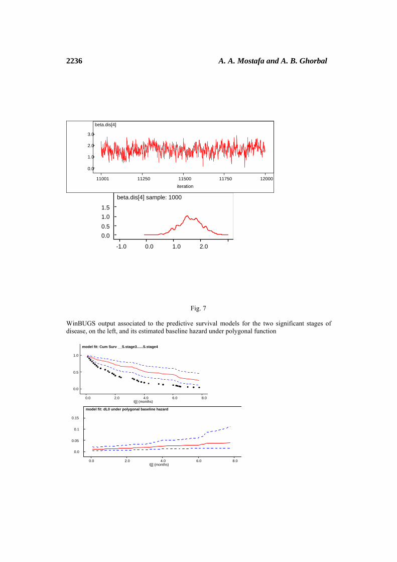
total 470.958 429.634 512.282 41.324 A simple summary (Table 7) can be generated showing posterior mean, median and standard deviation with 95% posterior credible interval. A fuller picture of the posterior distributions for the quantities of primary interest in the stochastic model is shown in Figures 6 and 7. Table 7 WinBUGS output for Larynx Cancer Data: posterior statistics

Node Mean SD MC error 2.5 % Median 97.5 % Start sample beta.dis[2] 0.02504 0.4642 0.02413 -0.9076 0.02229 0.9108 1001 11000 beta.dis[3] 0.6206 0.357 0.02658 -0.0768 0.5619 1.235 1001 11000 beta.dis[4] 1.615 0.4347 0.03089 0.7645 1.616 2.446 1001 11000

sigma 0.4252 0.07765 0.002168 0.3108 0.4129 0.6159 1001 11000


WinBUGS output associated to the coefficient of the covariate; the Stages for the Disease, on the left, and their estimated posterior density

beta.dis[2]

iteration11001 11250 11500 11750 12000

-2.0

-1.0

0.0

1.0

2.0

beta.dis[2] sample: 1000

-2.0 -1.0 0.0 1.0

0.0 0.25 0.5

0.75 1.0

beta.dis[3]

iteration11001 11250 11500 11750 12000

-1.0

0.0

1.0

2.0


-1.0 0.0 1.0

0.0 0.5 1.0 1.5

Fig. 6


beta.dis[4]

iteration11001 11250 11500 11750 12000

0.0

1.0

2.0

3.0


-1.0 0.0 1.0 2.0

0.0 0.5 1.0 1.5

WinBUGS output associated to the predictive survival models for the two significant stages of disease, on the left, and its estimated baseline hazard under polygonal function

model fit: Cum Surv __S.stage3......S.stage4

t[j] (months) 0.0 2.0 4.0 6.0 8.0

0.0

0.5

1.0

model fit: dL0 under polygonal baseline hazard

t[j] (months) 0.0 2.0 4.0 6.0 8.0

0.0

0.05

0.1

0.15

Fig. 7


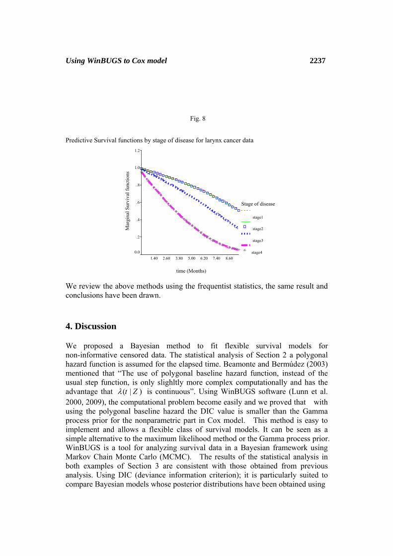
Predictive Survival functions by stage of disease for larynx cancer data

time (Months)

8.607.406.205.003.802.601.40

Mar

gina

l Sur

viva

l fun

ctio

ns

1.2

1.0

.8

.6

.4

.2

0.0

Stage of disease

stage1

stage2

stage3

stage4

We review the above methods using the frequentist statistics, the same result and conclusions have been drawn.

4. Discussion

We proposed a Bayesian method to fit flexible survival models for non-informative censored data. The statistical analysis of Section 2 a polygonal hazard function is assumed for the elapsed time. Beamonte and Bermúdez (2003) mentioned that “The use of polygonal baseline hazard function, instead of the usual step function, is only slighltly more complex computationally and has the advantage that ( | )t Zλ is continuous”. Using WinBUGS software (Lunn et al. 2000, 2009), the computational problem become easily and we proved that with using the polygonal baseline hazard the DIC value is smaller than the Gamma process prior for the nonparametric part in Cox model. This method is easy to implement and allows a flexible class of survival models. It can be seen as a simple alternative to the maximum likelihood method or the Gamma process prior. WinBUGS is a tool for analyzing survival data in a Bayesian framework using Markov Chain Monte Carlo (MCMC). The results of the statistical analysis in both examples of Section 3 are consistent with those obtained from previous analysis. Using DIC (deviance information criterion); it is particularly suited to compare Bayesian models whose posterior distributions have been obtained using

Fig. 8


MCMC. DIC has been implemented as a tool in the BUGS software package. However, much technical statistical knowledge is required for it to be used correctly. These programs provide an alternative platform that could be used to confirm results of ‘frequentist’ software. Bayesian inference has several advantages over the frequentist approaches, particularly in the flexibility of model-building for complex data. Moreover, for many models, ‘frequentist’ inference can be obtained as a special case of Bayesian inference with the use of non-informative priors (Ibrahim et al., 2001). The Bayesian approach enables us to make exact inference based on the posterior distribution for any sample size, whereas the 'frequentist' approach relies heavily on the large sample approximation, and there is always the issue of whether the sample size is large enough for the approximation to be valid (Ibrahim et al., 2001). There is a danger that the additional complexity of Bayesian methods could lead to improper data analysis if it is not used correctly. Although, this article proposed the prior elicitation for the baseline hazard in the Cox model, it is straightforward to extend to additive hazard model with simple modification in Display 1 (see e.g., Aalen, 1980). Moreover; this proposed article tried to solve what Silva and Amaral-Turkman (2004) said in their comments that “there are also further problems that need special attention, such as elicitation of priors). With the above mentioned advantages and the availability of the latest version 1.4.3 software WinBUGS, analysis of survival models is made possible and simple.

References [1] O. O. Aalen, Nonparametric inference in connection with multiple decrement

models. Statistical Research Report 6, Department of Mathematics, University of Oslo, 1972.

[2] O.O. Aalen, P.K. Andersen, Ø. Borgan, R.D. Gill, N. Keiding,. History of applications of martingales in survival analysis. Electronic Journal for History of Probability and Statist. 5, 1 (2009), 1–28. Available: http://www.emis.de/journals/JEHPS/juin2009/Aalenetal.pdf.

[3] B. Altshuler, Theory for the measurement of competing risks in animal experiements. Mathematical Biosciences, 6, (1970), 1–11.

[4] P.K. Andersen, and R.D. Gill,.Cox’s regression model for counting processes: A large sample study. Annals of Statistics, 10 (1982) , 1100–1120.

[5] E. Beamonte, and J. D. Bermúdez, A Bayesian semiparmetric analysis for additive hazards models with censored observations. Test, 12, 2 (2003), 101–117.

[6] J. G. Brahim, M. Chen, and D. Sinha, Bayesian Survival Analysis. Springer – Verlag, New York, 2001.

Using WinBUGS to Cox model 2239 [7] S.P. Brooks, Markov chain Monte Carlo method and its application. The

Statistician, 47 (1998), Part 1, 69–100. [8] D.Clayton. A Monte Carlo for Bayesian inference in frailty models.

Biometrics, 47, (1991), 467– 485. [9] D.Clayton, Bayesian analysis of frailty models. Technical Report, Medical

Research Council Biostatistics Unit, Cambridge, 1994. [10] D.R. Cox, Regression models and life tables (with discussion), Journal of the

Royal Statistical Society, Series B, 34 (1972), 187-220. [11] Cox, D.R. (1975). Partial likelihood. Biometrika, 62, 269–276. [12] P. Feigl, and M. Zelen, Estimation of exponential survival probabilities with

concomitant information, Biometrics, 21 (1965), 826–838. [13] D. Gamerman, Dynamic Bayesian models for Survival data, Applied

Statistics, 40 (1991), 63–79. [14] A. Gelman, and D. B. Rubin, Inference from iterative simulation using

multiple sequences, Statistical Science, 7 (1992), 457–511. [15] S. Geman, and D. Geman, Stochastic relaxation, Gibbs distribution and the

Bayesian restoration of images, IEEE Transactions on Pattern Analysis and Machine Intelligence, 6 (1984), 721–741.

[16] R. D. Gill, Product-integration, In Encyclopedia of Biostatistics (eds P. Armitage and T. Colton), 6 (2005), 4246 – 4250, Wiley, Chichester.

[17] S. Johansen, An extension of Cox’s regression model. International Statistical Review, 51 (1983),165 – 174.

[18] J. D. Kalbfleisch and R.L. Prentice, The statistical analysis of failure time data. Wiley, New York, 1980.

[19] J. D. Kalbfleisch, Nonparametric Bayesian analysis of survival time data. Journal of the Royal Statistical Society, Series B 40 (1978) , 214 – 221.

[20] Kaplan, E.L. and P. Meier, Non-parametric estimation from incomplete observations. Journal of the American Statistical Association, 53 (1958), 457– 481.

[21] O. Kardaun, Statistical analysis of male larynx-cancer patients – a case study. Statistical Nederlandica, 37 (1983), 103–126.

[22] D. Kumar, and B. Klefsjö, Proportional hazards model: a review, Reliability Engineering and System Safety, 44 (1994), 177–188.

[23] J. F. Lawless, Statistical Models and Methods for Lifetime Data. John Wiley and Sons, New York, 1982.

[24] D.J. Lunn, A . Thomas, N. Best, D. Spiegelhalter, WinBUGS – a Bayesian modelling framework: concepts, structure, and extensibility. Statistics and Computing ,10 (2000) , 325 – 337.

[25] D. J. Lunn, D. Spiegelhalter, A. Thomas, and N, Best. The BUGS project: Evolution, critique and future directions. Statistics in Medicine, 28 (2009), 3049 – 3067.

2240 A. A. Mostafa and A. B. Ghorbal [26] T.Næs, The asymptotic distribution of the estimator for the regression

Parameter in Cox’s regression model. Scandinavian Journal of Statistics, 9 (1982), 107–115.

[27] W. Nelson, Hazard plotting for incomplete failure data, Journal of Quality Technology, 1 (1969), 27 – 52.

[28] G. L. Silva, and M. A. Amaral-Turkman, Bayesian Analysis of an Additive Survival Model with Frailty. Communications in Statistics – Theory and Methods, 33 (10) (2004), 2517–2533.

[29] D. Sinha and D.K. Dey. Semiparametric Bayesian analysis of survival data. Journal of the American Statistical Association, 92 (1997), 1195 – 1212.

[30] D. Spiegelhalter, A. Thomas, N. Best, and W. Gilks, BUGS 0.5: Examples Volume 1, MRC Biostatistics Unit, Institute of Public Health, Cambridge, UK, 1996.

[31] D. Spiegelhalter, A. Thomas, N. Best, and D. Lunn, (2003), WinBUGS User Manual, Version 1.4, MRC Biostatistics Unit, Institute of Public Health and Department of Epidemiology and Public Health, Imperial College School of Medicine, UK, 2003, available at: http://www.mrc-bsu.cam.ac.uk/bugs

[32] A. A. Tsiatis, A large sample study of Cox’s regression model. Annals of Statistics, 9 (1981). 93 – 108.

Received: December, 2010

Documents

Using WinBUGS to Cox Model with Changing from the Baseline