Embed Size (px)
Citation preview
Using the PAC2002Tire ModelThe PAC2002 Magic-Formula tire model has been developed by MSC.Software according to Tyre and Vehicle Dynamics by Pacejka [1]. PAC2002 is latest version of a Magic-Formula model available in Adams/Tire.
Learn about:
• When to Use PAC2002
• Modeling of Tire-Road Interaction Forces
• Axis Systems and Slip Definitions
• Contact Point and Normal Load Calculation
• Basics of the Magic Formula in PAC2002
• Steady-State: Magic Formula in PAC2002
• Transient Behavior in PAC2002
• Gyroscopic Couple in PAC2002
• Left and Right Side Tires
• USE_MODES of PAC2002: from Simple to Complex
• Quality Checks for the Tire Model Parameters
• Standard Tire Interface (STI) for PAC2002
• Definitions
• References
• Example of PAC2002 Tire Property File
• Contact Methods
When to Use PAC2002Magic-Formula (MF) tire models are considered the state-of-the-art for modeling tire-road interaction forces in vehicle dynamics applications. Since 1987, Pacejka and others have published several versions of this type of tire model. The PAC2002 contains the latest developments that have been published in Tyre and Vehicle Dynamics by Pacejka [1].
In general, a MF tire model describes the tire behavior for rather smooth roads (road obstacle wavelengths longer than the tire radius) up to frequencies of 8 Hz. This makes the tire model applicable for all generic vehicle handling and stability simulations, including:
• Steady-state cornering
• Single- or double-lane change
• Braking or power-off in a turn
• Split-mu braking tests
• J-turn or other turning maneuvers
Adams/TireUsing the PAC2002Tire Model
2
• ABS braking, when stopping distance is important (not for tuning ABS control strategies)
• Other common vehicle dynamics maneuvers on rather smooth roads (wavelength of road obstacles must be longer than the tire radius)
For modeling roll-over of a vehicle, you must pay special attention to the overturning moment characteristics of the tire (Mx) and the loaded radius modeling. The last item may not be sufficiently
accurate in this model.
The PAC2002 model has proven to be applicable for car, truck, and aircraft tires with camber (inclination) angles to the road not exceeding 15 degrees.
PAC2002 and Previous Magic Formula Models
Compared to previous versions, PAC2002 is backward compatible with all previous versions of PAC2002, MF-Tyre 5.x tire models, and related tire property files.
New Features
The enhancements for PAC2002 in Adams/Tire 2005 r2 are:
• More advanced tire-transient modeling using a contact mass in the contact point with the road. This results in more realistic dynamic tire model response at large slip, low speed, and standstill (usemode > 20).
• Parking torque and turn-slip have been introduced: the torque around the vertical axis due to turning at standstill or at low speed (no need for extra parameters).
• Extended loaded radius modeling (see Contact Point and Normal Load Calculation) are suitable for driving under extreme conditions like roll-over events and racing applications.
• The option to use a nonlinear spline for the vertical tire load-deflection instead of a linear tire stiffness. See Contact Point and Normal Load Calculation.
• Modeling of bottoming of the tire to the road by using another spline for defining the bottoming forces. Learn more about wheel bottoming.
• Online scaling of the tire properties during a simulation; the scaling factors of the PAC2002 can now be changed as a function of time, position, or any other variable in your model dataset. See Online Scaling of Tire Properties.
Modeling of Tire-Road Interaction ForcesFor vehicle dynamics applications, an accurate knowledge of tire-road interaction forces is inevitable because the movements of a vehicle primarily depend on the road forces on the tires. These interaction forces depend on both road and tire properties, and the motion of the tire with respect to the road.
In the radial direction, the MF tire models consider the tire to behave as a parallel linear spring and linear damper with one point of contact with the road surface. The contact point is determined by considering the tire and wheel as a rigid disc. In the contact point between the tire and the road, the contact forces in

3Using the PAC2002Tire Model
longitudinal and lateral direction strongly depend on the slip between the tire patch elements and the road.
The figure, Input and Output Variables of the Magic Formula Tire Model, presents the input and output vectors of the PAC2002 tire model. The tire model subroutine is linked to the Adams/Solver through the Standard Tire Interface (STI) [3]. The input through the STI consists of:
• Position and velocities of the wheel center
• Orientation of the wheel
• Tire model (MF) parameters
• Road parameters
The tire model routine calculates the vertical load and slip quantities based on the position and speed of the wheel with respect to the road. The input for the Magic Formula consists of the wheel load (Fz), the
longitudinal and lateral slip , and inclination angle with the road. The output is the forces (Fx,
Fy) and moments (Mx, My, Mz) in the contact point between the tire and the road. For calculating these
forces, the MF equations use a set of MF parameters, which are derived from tire testing data.
The forces and moments out of the Magic Formula are transferred to the wheel center and returned to Adams/Solver through STI.
Input and Output Variables of the Magic Formula Tire Model
Axis Systems and Slip Definitions• Axis Systems

Adams/TireUsing the PAC2002Tire Model
4
• Units
• Definition of Tire Slip Quantities
Axis Systems
The PAC2002 model is linked to Adams/Solver using the TYDEX STI conventions, as described in the TYDEX-Format [2] and the STI [3].
The STI interface between the PAC2002 model and Adams/Solver mainly passes information to the tire model in the C-axis coordinate system. In the tire model itself, a conversion is made to the W-axis system because all the modeling of the tire behavior as described in this help assumes to deal with the slip quantities, orientation, forces, and moments in the contact point with the TYDEX W-axis system. Both axis systems have the ISO orientation but have different origin as can be seen in the figure below.
TYDEX C- and W-Axis Systems Used in PAC2002, Source [2]
The C-axis system is fixed to the wheel carrier with the longitudinal xc-axis parallel to the road and in
the wheel plane (xc-zc-plane). The origin of the C-axis system is the wheel center.
The origin of the W-axis system is the road contact-point defined by the intersection of the wheel plane, the plane through the wheel carrier, and the road tangent plane.
The forces and moments calculated by PAC2002 using the MF equations in this guide are in the W-axis system. A transformation is made in the source code to return the forces and moments through the STI to Adams/Solver.
The inclination angle is defined as the angle between the wheel plane and the normal to the road tangent plane (xw-yw-plane).

5Using the PAC2002Tire Model
Units
The units of information transferred through the STI between Adams/Solver and PAC2002 are according to the SI unit system. Also, the equations for PAC2002 described in this guide have been developed for use with SI units, although you can easily switch to another unit system in your tire property file. Because of the non-dimensional parameters, only a few parameters have to be changed.
However, the parameters in the tire property file must always be valid for the TYDEX W-axis system (ISO oriented). The basic SI units are listed in the table below (also see Definitions).
SI Units Used in PAC2002
Definition of Tire Slip Quantities
The longitudinal slip velocity Vsx in the contact point (W-axis system, see Slip Quantities at Combined
Cornering and Braking/Traction) is defined using the longitudinal speed Vx, the wheel rotational velocity
, and the effective rolling radius Re:
(1)
Variable type: Name: Abbreviation: Unit:
Angle Slip angle
Inclination angle
Radians
Force Longitudinal force
Lateral force
Vertical load
Fx
Fy
Fz
Newton
Moment Overturning moment
Rolling resistance moment
Self-aligning moment
Mx
My
Mz
Newton.meter
Speed Longitudinal speed
Lateral speed
Longitudinal slip speed
Lateral slip speed
Vx
Vy
Vsx
Vsy
Meters per second
Rotational speed Tire rolling speed Radians per second
Vsx Vx Re–=
Adams/TireUsing the PAC2002Tire Model
6
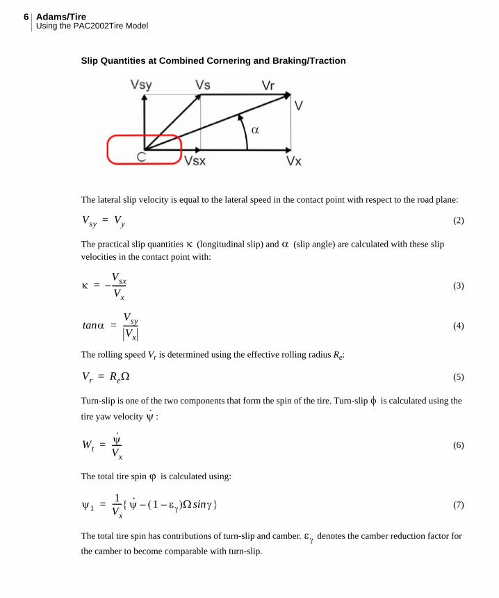
Slip Quantities at Combined Cornering and Braking/Traction
The lateral slip velocity is equal to the lateral speed in the contact point with respect to the road plane:
(2)
The practical slip quantities (longitudinal slip) and (slip angle) are calculated with these slip velocities in the contact point with:
(3)
(4)
The rolling speed Vr is determined using the effective rolling radius Re:
(5)
Turn-slip is one of the two components that form the spin of the tire. Turn-slip is calculated using the
tire yaw velocity :
(6)
The total tire spin is calculated using:
(7)
The total tire spin has contributions of turn-slip and camber. denotes the camber reduction factor for
the camber to become comparable with turn-slip.
Vsy Vy=
Vsx
Vx-------–=
tanVsy
Vx--------=
Vr Re=
·
Wt·
Vx-----=
11Vx----- · 1 – sin– =

7Using the PAC2002Tire Model
Contact Point and Normal Load Calculation• Contact Point
• Loaded and Effective Tire Rolling Radius
• Wheel Bottoming
Contact Point
In the vertical direction, the tire is modeled as a parallel linear spring and damper having one point of contact (C) with the road. This is valid for road obstacles with a wavelength larger than the tire radius (for example, for car tires 1m).
For calculating the kinematics of the tire relative to the road, the road is approximated by its tangent plane at the road point right below the wheel center (see the figure below).
Contact Point C: Intersection between Road Tangent Plane, Spin Axis Plane, and Wheel Plane
The contact point is determined by the line of intersection of the wheel center-plane with the road tangent (ground) plane and the line of intersection of the wheel center-plane with the plane through the wheel spin axis.
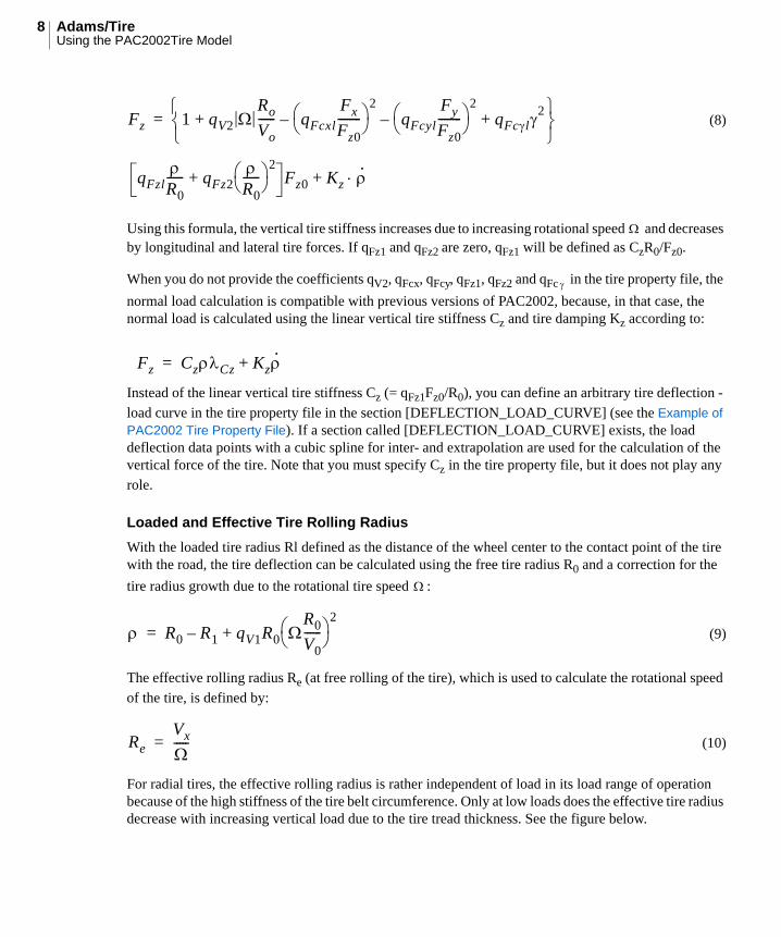
The normal load Fz of the tire is calculated with the tire deflection as follows:
Adams/TireUsing the PAC2002Tire Model
8
(8)
Using this formula, the vertical tire stiffness increases due to increasing rotational speed and decreases by longitudinal and lateral tire forces. If qFz1 and qFz2 are zero, qFz1 will be defined as CzR0/Fz0.
When you do not provide the coefficients qV2, qFcx, qFcy, qFz1, qFz2 and qFc in the tire property file, the
normal load calculation is compatible with previous versions of PAC2002, because, in that case, the normal load is calculated using the linear vertical tire stiffness Cz and tire damping Kz according to:
Instead of the linear vertical tire stiffness Cz (= qFz1Fz0/R0), you can define an arbitrary tire deflection -
load curve in the tire property file in the section [DEFLECTION_LOAD_CURVE] (see the Example of PAC2002 Tire Property File). If a section called [DEFLECTION_LOAD_CURVE] exists, the load deflection data points with a cubic spline for inter- and extrapolation are used for the calculation of the vertical force of the tire. Note that you must specify Cz in the tire property file, but it does not play any
role.
Loaded and Effective Tire Rolling Radius
With the loaded tire radius Rl defined as the distance of the wheel center to the contact point of the tire with the road, the tire deflection can be calculated using the free tire radius R0 and a correction for the
tire radius growth due to the rotational tire speed :
(9)
The effective rolling radius Re (at free rolling of the tire), which is used to calculate the rotational speed
of the tire, is defined by:
(10)
For radial tires, the effective rolling radius is rather independent of load in its load range of operation because of the high stiffness of the tire belt circumference. Only at low loads does the effective tire radius decrease with increasing vertical load due to the tire tread thickness. See the figure below.
Fz 1 qV2 Ro
Vo------ qFcxl
Fx
Fz0--------
2
– qFcyl
Fy
Fz0--------
2
– qFcl2
+ +
qFzlR0------ qFz2
R0------ 2
+ Fz0 Kz ·+
=
Fz CzCz Kz·+=
R0 R1– qV1R0 R0
V0------
2
+=
ReVx
-----=
9Using the PAC2002Tire Model
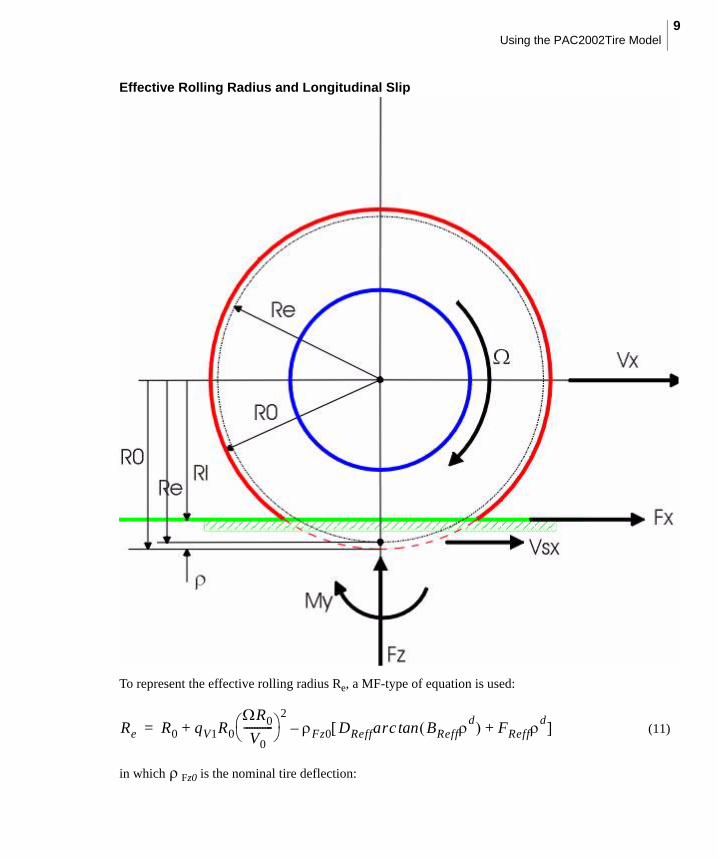
Effective Rolling Radius and Longitudinal Slip
To represent the effective rolling radius Re, a MF-type of equation is used:
(11)
in which Fz0 is the nominal tire deflection:
Re R0 qV1R0
R0
V0-----------
2Fz0 DReffarc BReff
d FReffd
+tan –+=

Adams/TireUsing the PAC2002Tire Model
10
(12)
and is called the dimensionless radial tire deflection, defined by:
(13)
Example of Loaded and Effective Tire Rolling Radius as Function of Vertical Load
Normal Load and Rolling Radius Parameters
Name: Name Used in Tire Property File: Explanation:
Fz0 FNOMIN Nominal wheel load
Ro UNLOADED_RADIUS Free tire radius
BReff BREFF Low load stiffness effective rolling radius
DReff DREFF Peak value of effective rolling radius
FReff FREFF High load stiffness effective rolling radius
Cz VERTICAL_STIFFNESS Tire vertical stiffness (if qFz1=0)
Fz0
Fz0
CzCz---------------=
d
d Fz0
---------=
11Using the PAC2002Tire Model
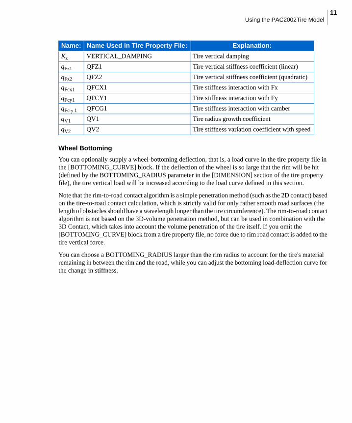
Wheel Bottoming
You can optionally supply a wheel-bottoming deflection, that is, a load curve in the tire property file in the [BOTTOMING_CURVE] block. If the deflection of the wheel is so large that the rim will be hit (defined by the BOTTOMING_RADIUS parameter in the [DIMENSION] section of the tire property file), the tire vertical load will be increased according to the load curve defined in this section.
Note that the rim-to-road contact algorithm is a simple penetration method (such as the 2D contact) based on the tire-to-road contact calculation, which is strictly valid for only rather smooth road surfaces (the length of obstacles should have a wavelength longer than the tire circumference). The rim-to-road contact algorithm is not based on the 3D-volume penetration method, but can be used in combination with the 3D Contact, which takes into account the volume penetration of the tire itself. If you omit the [BOTTOMING_CURVE] block from a tire property file, no force due to rim road contact is added to the tire vertical force.
You can choose a BOTTOMING_RADIUS larger than the rim radius to account for the tire's material remaining in between the rim and the road, while you can adjust the bottoming load-deflection curve for the change in stiffness.
Kz VERTICAL_DAMPING Tire vertical damping
qFz1 QFZ1 Tire vertical stiffness coefficient (linear)
qFz2 QFZ2 Tire vertical stiffness coefficient (quadratic)
qFcx1 QFCX1 Tire stiffness interaction with Fx
qFcy1 QFCY1 Tire stiffness interaction with Fy
qFc 1 QFCG1 Tire stiffness interaction with camber
qV1 QV1 Tire radius growth coefficient
qV2 QV2 Tire stiffness variation coefficient with speed
Name: Name Used in Tire Property File: Explanation:

Adams/TireUsing the PAC2002Tire Model
12
If (Pentire - (Rtire - Rbottom) - ½·width ·| tan() |) < 0, the left or right side of the rim has contact with the
road. Then, the rim deflection Penrim can be calculated using:
= max(0 , ½·width ·| tan( ) | ) + Pentire- (Rtire - Rbottom)
Penrim= /(2 · width ·| tan( ) |)
2
13Using the PAC2002Tire Model
Srim= ½·width - max(width , /| tan( ) |)/3
with Srim, the lateral offset of the force with respect to the wheel plane.
If the full rim has contact with the road, the rim deflection is:
Penrim = Pentire - (Rtire - Rbottom)
Srim = width2 · | tan( ) | · /(12 · Penrim)
Using the load - deflection curve defined in the [BOTTOMING_CURVE] section of the tire property file, the additional vertical force due to the bottoming is calculated, while Srim multiplied by the sign of the
inclination is used to calculate the contribution of the bottoming force to the overturning moment. Further, the increase of the total wheel load Fz due to the bottoming (Fzrim) will not be taken into account
in the calculation for Fx, Fy, My, and Mz. Fzrim will only contribute to the overturning moment Mx using
the Fzrim·Srim.
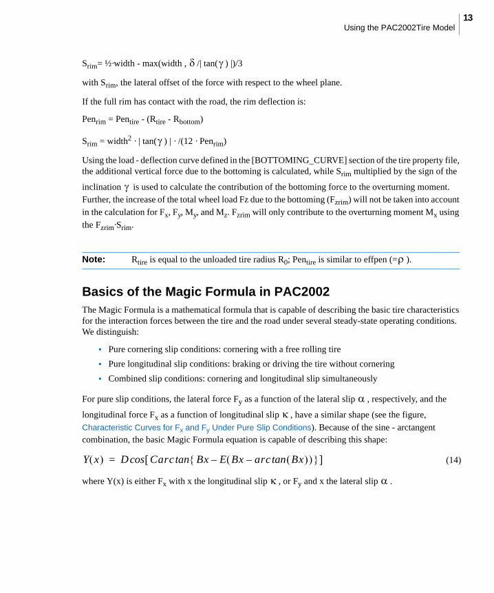
Basics of the Magic Formula in PAC2002The Magic Formula is a mathematical formula that is capable of describing the basic tire characteristics for the interaction forces between the tire and the road under several steady-state operating conditions. We distinguish:
• Pure cornering slip conditions: cornering with a free rolling tire
• Pure longitudinal slip conditions: braking or driving the tire without cornering
• Combined slip conditions: cornering and longitudinal slip simultaneously
For pure slip conditions, the lateral force Fy as a function of the lateral slip , respectively, and the
longitudinal force Fx as a function of longitudinal slip , have a similar shape (see the figure,
Characteristic Curves for Fx and Fy Under Pure Slip Conditions). Because of the sine - arctangent combination, the basic Magic Formula equation is capable of describing this shape:
(14)
where Y(x) is either Fx with x the longitudinal slip , or Fy and x the lateral slip .
Note: Rtire is equal to the unloaded tire radius R0; Pentire is similar to effpen (= ).
Y x D Carc Bx E Bx arc Bx tan– – tan cos=
Adams/TireUsing the PAC2002Tire Model
14
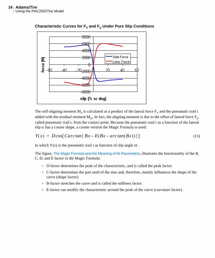
Characteristic Curves for Fx and Fy Under Pure Slip Conditions
The self-aligning moment Mz is calculated as a product of the lateral force Fy and the pneumatic trail t
added with the residual moment Mzr. In fact, the aligning moment is due to the offset of lateral force Fy,
called pneumatic trail t, from the contact point. Because the pneumatic trail t as a function of the lateral slip has a cosine shape, a cosine version the Magic Formula is used:
(15)
in which Y(x) is the pneumatic trail t as function of slip angle .
The figure, The Magic Formula and the Meaning of Its Parameters, illustrates the functionality of the B, C, D, and E factor in the Magic Formula:
• D-factor determines the peak of the characteristic, and is called the peak factor.
• C-factor determines the part used of the sine and, therefore, mainly influences the shape of the curve (shape factor).
• B-factor stretches the curve and is called the stiffness factor.
• E-factor can modify the characteristic around the peak of the curve (curvature factor).
Y x D Carc Bx E Bx arc Bx tan– – tan cos=
15Using the PAC2002Tire Model
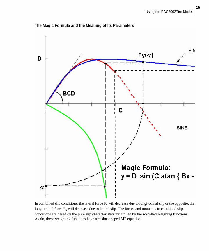
The Magic Formula and the Meaning of Its Parameters
In combined slip conditions, the lateral force Fy will decrease due to longitudinal slip or the opposite, the
longitudinal force Fx will decrease due to lateral slip. The forces and moments in combined slip
conditions are based on the pure slip characteristics multiplied by the so-called weighing functions. Again, these weighting functions have a cosine-shaped MF equation.
Adams/TireUsing the PAC2002Tire Model
16
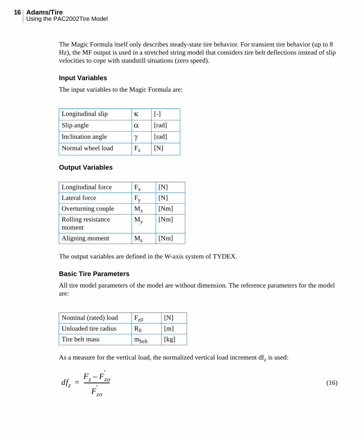
The Magic Formula itself only describes steady-state tire behavior. For transient tire behavior (up to 8 Hz), the MF output is used in a stretched string model that considers tire belt deflections instead of slip velocities to cope with standstill situations (zero speed).
Input Variables
The input variables to the Magic Formula are:
Output Variables
The output variables are defined in the W-axis system of TYDEX.
Basic Tire Parameters
All tire model parameters of the model are without dimension. The reference parameters for the model are:
As a measure for the vertical load, the normalized vertical load increment dfz is used:
(16)
Longitudinal slip [-]
Slip angle [rad]
Inclination angle [rad]
Normal wheel load Fz [N]
Longitudinal force Fx [N]
Lateral force Fy [N]
Overturning couple Mx [Nm]
Rolling resistance moment
My [Nm]
Aligning moment Mz [Nm]
Nominal (rated) load Fz0 [N]
Unloaded tire radius R0 [m]
Tire belt mass mbelt [kg]
dfz
Fz Fzo
–
Fzo
-------------------=
17Using the PAC2002Tire Model
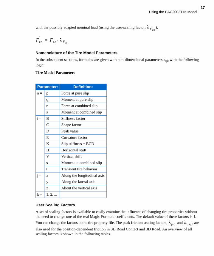
with the possibly adapted nominal load (using the user-scaling factor, ):
Nomenclature of the Tire Model Parameters
In the subsequent sections, formulas are given with non-dimensional parameters aijk with the following
logic:
Tire Model Parameters
User Scaling Factors
A set of scaling factors is available to easily examine the influence of changing tire properties without the need to change one of the real Magic Formula coefficients. The default value of these factors is 1.
You can change the factors in the tire property file. The peak friction scaling factors, and , are
also used for the position-dependent friction in 3D Road Contact and 3D Road. An overview of all scaling factors is shown in the following tables.
Parameter: Definition:
a = p Force at pure slip
q Moment at pure slip
r Force at combined slip
s Moment at combined slip
i = B Stiffness factor
C Shape factor
D Peak value
E Curvature factor
K Slip stiffness = BCD
H Horizontal shift
V Vertical shift
s Moment at combined slip
t Transient tire behavior
j = x Along the longitudinal axis
y Along the lateral axis
z About the vertical axis
k = 1, 2, ...
FZ0
Fzo
Fzo Fz0=
Adams/TireUsing the PAC2002Tire Model
18
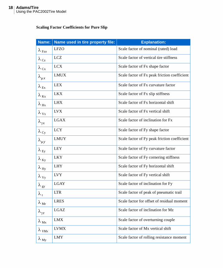
Scaling Factor Coefficients for Pure Slip
Name: Name used in tire property file: Explanation:
FzoLFZO Scale factor of nominal (rated) load
CzLCZ Scale factor of vertical tire stiffness
CxLCX Scale factor of Fx shape factor
LMUX Scale factor of Fx peak friction coefficient
ExLEX Scale factor of Fx curvature factor
KxLKX Scale factor of Fx slip stiffness
HxLHX Scale factor of Fx horizontal shift
VxLVX Scale factor of Fx vertical shift
LGAX Scale factor of inclination for Fx
CyLCY Scale factor of Fy shape factor
LMUY Scale factor of Fy peak friction coefficient
EyLEY Scale factor of Fy curvature factor
KyLKY Scale factor of Fy cornering stiffness
HyLHY Scale factor of Fy horizontal shift
VyLVY Scale factor of Fy vertical shift
gyLGAY Scale factor of inclination for Fy
tLTR Scale factor of peak of pneumatic trail
MrLRES Scale factor for offset of residual moment
LGAZ Scale factor of inclination for Mz
MxLMX Scale factor of overturning couple
VMxLVMX Scale factor of Mx vertical shift
MyLMY Scale factor of rolling resistance moment
x
x
y
z

19Using the PAC2002Tire Model
Scaling Factor Coefficients for Combined Slip
Scaling Factor Coefficients for Transient Response
Note that the scaling factors change during the simulation according to any user-introduced function. See the next section, Online Scaling of Tire Properties.
Online Scaling of Tire Properties
PAC2002 can provide online scaling of tire properties. For each scaling factor, a variable should be introduced in the Adams .adm dataset. For example:
!lfz0 scaling! adams_view_name='TR_Front_Tires until wheel_lfz0_var'VARIABLE/53, IC = 1, FUNCTION = 1.0
This lets you change the scaling factor during a simulation as a function of time or any other variable in your model. Therefore, tire properties can change because of inflation pressure, road friction, road temperature, and so on.
You can also use the scaling factors in co-simulations in MATLAB/Simulink.
For more detailed information, see Knowledge Base Article 12732.
Steady-State: Magic Formula in PAC2002• Steady-State Pure Slip
Name: Name used in tire property file: Explanation:
xLXAL Scale factor of alpha influence on Fx
yLYKA Scale factor of alpha influence on Fx
VyLVYKA Scale factor of kappa-induced Fy
LS Scale factor of moment arm of Fx
Name: Name used in tire property file: Explanation:
LSGKP Scale factor of relaxation length of Fx
LSGAL Scale factor of relaxation length of Fy
gyrLGYR Scale factor of gyroscopic moment
s
Adams/TireUsing the PAC2002Tire Model
20
• Steady-State Combined Slip
Steady-State Pure Slip• Longitudinal Force at Pure Slip
• Lateral Force at Pure Slip
• Aligning Moment at Pure Slip
• Turn-slip and Parking
Formulas for the Longitudinal Force at Pure Slip
For the tire rolling on a straight line with no slip angle, the formulas are:
(17)
(18)
(19)
(20)
with following coefficients:
(21)
(22)
(23)
(24)
the longitudinal slip stiffness:
(25)
(26)
(27)
(28)
Fx Fx0 Fz =
Fx0 Dx Cxarc Bxx Ex Bxx arc Bxx tan– – tan SVx+ sin=
x SHx+=
x x=
Cx pCx1 Cx=
Dx x Fz 1 =
x pDx1 pDx2 fzd+ 1 pDx3 2– x=
Ex pEx1 pEx2 fzd pEx3 fz2
d+ + 1 pEx4 x sgn– Ex with Ex 1 =
Kx Fz pKx1 pKx2 fzd+ pKx3 fzd Kxexp =
Kx BxCxDx xFx0at x 0= = =
Bx Kx CxDx =
SHx pHx1 pHx2 dfz+ Hx=
SVx Fz pVx1 pVx2 dfz+ Vx x 1 =
21Using the PAC2002Tire Model
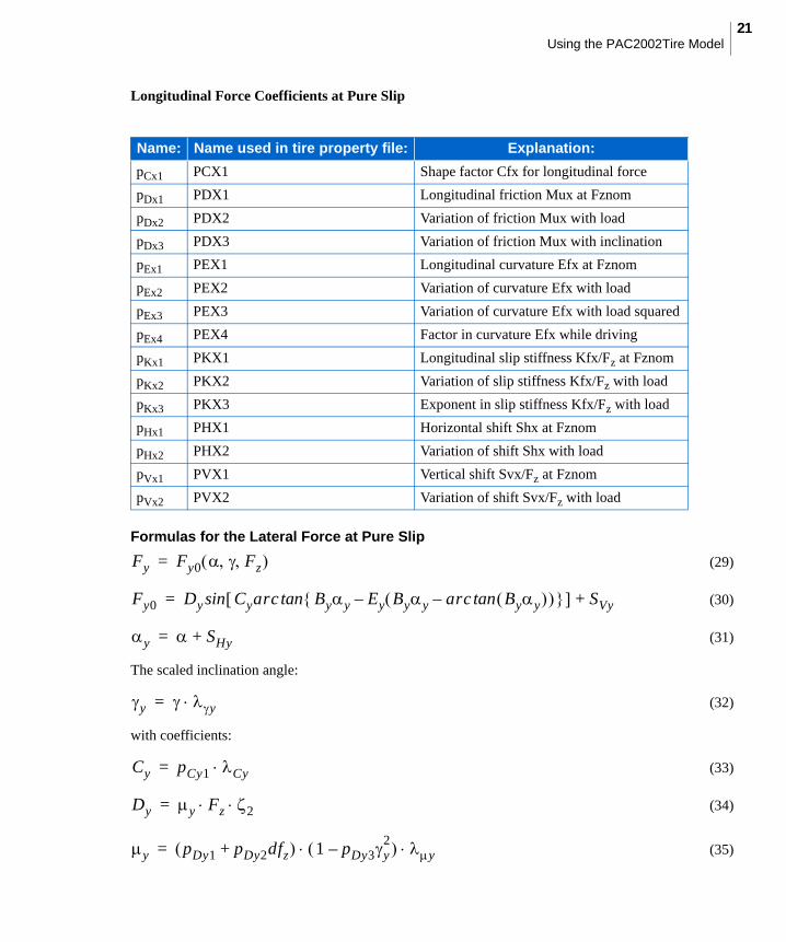
Longitudinal Force Coefficients at Pure Slip
Formulas for the Lateral Force at Pure Slip
(29)
(30)
(31)
The scaled inclination angle:
(32)
with coefficients:
(33)
(34)
(35)
Name: Name used in tire property file: Explanation:
pCx1 PCX1 Shape factor Cfx for longitudinal force
pDx1 PDX1 Longitudinal friction Mux at Fznom
pDx2 PDX2 Variation of friction Mux with load
pDx3 PDX3 Variation of friction Mux with inclination
pEx1 PEX1 Longitudinal curvature Efx at Fznom
pEx2 PEX2 Variation of curvature Efx with load
pEx3 PEX3 Variation of curvature Efx with load squared
pEx4 PEX4 Factor in curvature Efx while driving
pKx1 PKX1 Longitudinal slip stiffness Kfx/Fz at Fznom
pKx2 PKX2 Variation of slip stiffness Kfx/Fz with load
pKx3 PKX3 Exponent in slip stiffness Kfx/Fz with load
pHx1 PHX1 Horizontal shift Shx at Fznom
pHx2 PHX2 Variation of shift Shx with load
pVx1 PVX1 Vertical shift Svx/Fz at Fznom
pVx2 PVX2 Variation of shift Svx/Fz with load
Fy Fy0 Fz =
Fy0 Dy Cyarc Byy Ey Byy arc Byy tan– – tan SVy+sin=
y SHy+=
y y=
Cy pCy1 Cy=
Dy y Fz 2 =
y pDy1 pDy2dfz+ 1 pDy3y2
– y =
Adams/TireUsing the PAC2002Tire Model
22
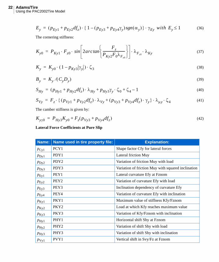
(36)
The cornering stiffness:
(37)
(38)
(39)
(40)
(41)
The camber stiffness is given by:
(42)
Lateral Force Coefficients at Pure Slip
Name: Name used in tire property file: Explanation:
pCy1 PCY1 Shape factor Cfy for lateral forces
pDy1 PDY1 Lateral friction Muy
pDy2 PDY2 Variation of friction Muy with load
pDy3 PDY3 Variation of friction Muy with squared inclination
pEy1 PEY1 Lateral curvature Efy at Fznom
pEy2 PEY2 Variation of curvature Efy with load
pEy3 PEY3 Inclination dependency of curvature Efy
pEy4 PEY4 Variation of curvature Efy with inclination
pKy1 PKY1 Maximum value of stiffness Kfy/Fznom
pKy2 PKY2 Load at which Kfy reaches maximum value
pKy3 PKY3 Variation of Kfy/Fznom with inclination
pHy1 PHY1 Horizontal shift Shy at Fznom
pHy2 PHY2 Variation of shift Shy with load
pHy3 PHY3 Variation of shift Shy with inclination
pVy1 PVY1 Vertical shift in Svy/Fz at Fznom
Ey pEy1 pEy2dfz+ 1 pEy3 pEy4y+ y sgn– Ey with Ey 1 =
Ky0 PKy1 Fz0 2arcFz
PKy2F0Fz0
---------------------------
tan Fz0Ky sin =
Ky Ky0 1 pKy3 y– 3 =
By Ky CyDy =
SHy pHy1 pHy2dfz+ Hy pHy3y 0 4 1–++=
SVy Fz pVy1 pVy2dfz+ Vy pVy3 pVy4dfz+ y+ y 4 =
Ky0 PHy3Ky0 Fz pVy3 pVy4dfz+ +=
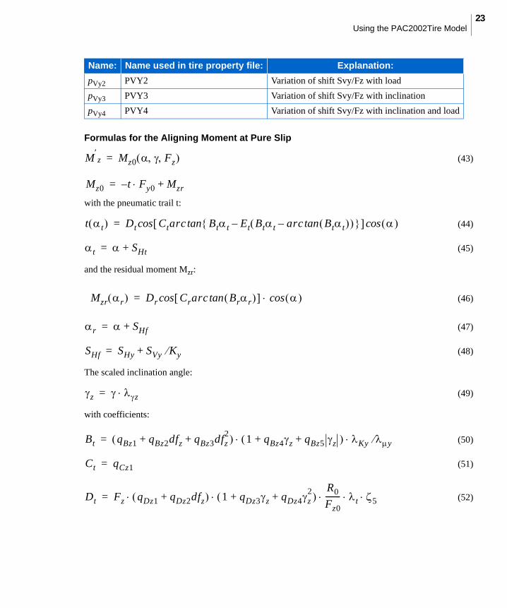
23Using the PAC2002Tire Model
Formulas for the Aligning Moment at Pure Slip
(43)
with the pneumatic trail t:
(44)
(45)
and the residual moment Mzr:
(46)
(47)
(48)
The scaled inclination angle:
(49)
with coefficients:
(50)
(51)
(52)
pVy2 PVY2 Variation of shift Svy/Fz with load
pVy3 PVY3 Variation of shift Svy/Fz with inclination
pVy4 PVY4 Variation of shift Svy/Fz with inclination and load
Name: Name used in tire property file: Explanation:
Mz Mz0 Fz =
Mz0 t Fy0 Mzr+–=
t t Dt Ctarc Btt Et Btt arc Btt tan– – tan coscos=
t SHt+=
Mzr r Dr Crarc Brr tan coscos=
r SHf+=
SHf SHy SVy Ky+=
z z=
Bt qBz1 qBz2dfz qBz3dfz2
+ + 1 qBz4z qBz5 z+ + Ky y =
Ct qCz1=
Dt Fz qDz1 qDz2dfz+ 1 qDz3z qDz4z2
+ + R0
Fz0-------- t 5 =
Adams/TireUsing the PAC2002Tire Model
24
(53)
(54)
(55)
(56)
An approximation for the aligning moment stiffness reads:
(57)
Aligning Moment Coefficients at Pure Slip
Name: Name used in tire property file: Explanation:
qBz1 QBZ1 Trail slope factor for trail Bpt at Fznom
qBz2 QBZ2 Variation of slope Bpt with load
qBz3 QBZ3 Variation of slope Bpt with load squared
qBz4 QBZ4 Variation of slope Bpt with inclination
qBz5 QBZ5 Variation of slope Bpt with absolute inclination
qBz9 QBZ9 Slope factor Br of residual moment Mzr
qBz10 QBZ10 Slope factor Br of residual moment Mzr
qCz1 QCZ1 Shape factor Cpt for pneumatic trail
qDz1 QDZ1 Peak trail Dpt = Dpt*(Fz/Fznom*R0)
qDz2 QDZ2 Variation of peak Dpt with load
qDz3 QDZ3 Variation of peak Dpt with inclination
qDz4 QDZ4 Variation of peak Dpt with inclination squared.
qDz6 QDZ6 Peak residual moment Dmr = Dmr/ (Fz*R0)
qDz7 QDZ7 Variation of peak factor Dmr with load
qDz8 QDZ8 Variation of peak factor Dmr with inclination
Et qEz1 qEz2dfz qEz3dfz2
+ + =
1 qEz4 qEz5z+ 2--- arc Bt Ct t tan +
w ith Et 1
SHt qHz1 qHz2dfz qHz3 qHz4 dfz+ z+ +=
Br qBz9Ky
y-------- qBz10 By Cy +
6=
Cr 7=
Dr Fz qDz6 qDz7dfz+ r qDz8 qDz9dfz+ z+ Ro 8 1–+ =
Kz t KyMz
----------– at
– 0 = =
25Using the PAC2002Tire Model
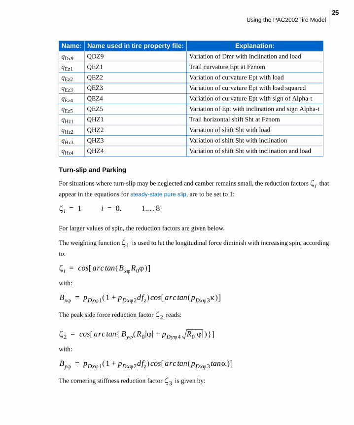
Turn-slip and Parking
For situations where turn-slip may be neglected and camber remains small, the reduction factors that
appear in the equations for steady-state pure slip, are to be set to 1:
For larger values of spin, the reduction factors are given below.
The weighting function is used to let the longitudinal force diminish with increasing spin, according
to:
with:
The peak side force reduction factor reads:
with:
The cornering stiffness reduction factor is given by:
qDz9 QDZ9 Variation of Dmr with inclination and load
qEz1 QEZ1 Trail curvature Ept at Fznom
qEz2 QEZ2 Variation of curvature Ept with load
qEz3 QEZ3 Variation of curvature Ept with load squared
qEz4 QEZ4 Variation of curvature Ept with sign of Alpha-t
qEz5 QEZ5 Variation of Ept with inclination and sign Alpha-t
qHz1 QHZ1 Trail horizontal shift Sht at Fznom
qHz2 QHZ2 Variation of shift Sht with load
qHz3 QHZ3 Variation of shift Sht with inclination
qHz4 QHZ4 Variation of shift Sht with inclination and load
Name: Name used in tire property file: Explanation:
i
i 1= i 0.= 1.8
1
i arc BxR0 tan cos=
Bx pDx1 1 pDx2dfz+ arc pDx3 tan cos=
2
2 arc By R0 pDy4 R0 + tan cos=
By pDx1 1 pDx2dfz+ arc pDx3 tan tan cos=
3

Adams/TireUsing the PAC2002Tire Model
26
The horizontal shift of the lateral force due to spin is given by:
The factors are defined by:
The spin force stiffness KyR0 is related to the camber stiffness Kyy0:
in which the camber reduction factor is given by:
The reduction factors and for the vertical shift of the lateral force are given by:
The reduction factor for the residual moment reads:
The peak spin torque Dr is given by:
3 arc pKy1R022 tan cos=
SHy DHy CHyarc BHyRo EHy BHyR0 arc BHyR0 tan– – tan sin=
CHy pHy1
DHy pHy2 pHy3dfz+ Vx
EHy
sin
PHy4
BHyKyR0
CyDyKy0----------------------
=
=
=
=
KyR0
Ky0
1 –-------------=
p1 1 p2dfz+ =
0 4
0 0
4 1 SHy SVy Ky–+
=
=
8 1 Dr+=
Dr DDr e CDrarc BDrR0 EDr BDrR0 arc BDrR0 tan– – tan sin=

27Using the PAC2002Tire Model
The maximum value is given by:
The pneumatic trail reduction factor due to turn slip is given by:
The moment at vanishing wheel speed at constant turning is given by:
The shape factors are given by:
in which:
The reduction factor reads:
The spin moment at 90º slip angle is given by:
The spin moment at 90º slip angle is multiplied by the weighing function to account for the action
of the longitudinal slip (see steady-state combined slip equations).
The reduction factor is given by:
DDrMz
2---CDr sin
-----------------------------=
5 arc qDt1R0 tan cos=
Mz qCr1yR0Fz Fz Fz0=
CDr qDr1
EDr qDr2
BDrKzr0
CDrDDr 1 y– --------------------------------------------
=
=
=
Kzr0 FzR0 qDz8 qDz9dfz+ =
6
6 arc qBr1R0 tan cos=
Mz90 Mz2--- arc qCr2R0 Gyx tan =
Gy
7

Adams/TireUsing the PAC2002Tire Model
28
Turn-Slip and Parking Parameters
The tire model parameters for turn-slip and parking are estimated automatically. In addition, you can specify each parameter individually in the tire property file (see example).
See KB-article ## for further details about parking by means of an example.
Name:Name used in
tire property file: Explanation:
p 1 PECP1 Camber spin reduction factor parameter in camber stiffness
p 2 PECP2 Camber spin reduction factor varying with load parameter in camber stiffness
pDx 1 PDXP1 Peak Fx reduction due to spin parameter
pDx 2 PDXP2 Peak Fx reduction due to spin with varying load parameter
pDx 3 PDXP3 Peak Fx reduction due to spin with kappa parameter
pDy 1 PDYP1 Peak Fy reduction due to spin parameter
pDy 2 PDYP2 Peak Fy reduction due to spin with varying load parameter
pDy 3 PDYP3 Peak Fy reduction due to spin with alpha parameter
pDy 4 PDYP4 Peak Fy reduction due to square root of spin parameter
pKy 1 PKYP1 Cornering stiffness reduction due to spin
pHy 1 PHYP1 Fy-alpha curve lateral shift limitation
pHy 2 PHYP2 Fy-alpha curve maximum lateral shift parameter
pHy 3 PHYP3 Fy-alpha curve maximum lateral shift varying with load parameter
pHy 4 PHYP4 Fy-alpha curve maximum lateral shift parameter
qDt 1 QDTP1 Pneumatic trail reduction factor due to turn slip parameter
qBr 1 QBRP1 Residual (spin) torque reduction factor parameter due to side slip
qCr 1 QCRP1 Turning moment at constant turning and zero forward speed parameter
qCr 2 QCRP2 Turn slip moment (at alpha=90deg) parameter for increase with spin
qDr 1 QDRP1 Turn slip moment peak magnitude parameter
qDr 2 QDRP2 Turn slip moment peak position parameter
72--- arc Mz90 DDr cos=
29Using the PAC2002Tire Model
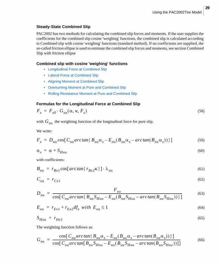
Steady-State Combined Slip
PAC2002 has two methods for calculating the combined slip forces and moments. If the user supplies the coefficients for the combined slip cosine 'weighing' functions, the combined slip is calculated according to Combined slip with cosine 'weighing' functions (standard method). If no coefficients are supplied, the so-called friction ellipse is used to estimate the combined slip forces and moments, see section Combined Slip with friction ellipse
Combined slip with cosine 'weighing' functions• Longitudinal Force at Combined Slip
• Lateral Force at Combined Slip
• Aligning Moment at Combined Slip
• Overturning Moment at Pure and Combined Slip
• Rolling Resistance Moment at Pure and Combined Slip
Formulas for the Longitudinal Force at Combined Slip
(58)
with the weighting function of the longitudinal force for pure slip.
We write:
(59)
(60)
with coefficients:
(61)
(62)
(63)
(64)
(65)
The weighting function follows as:
(66)
Fx Fx0 Gx Fz =
Gx
Fx Dx Cxarc Bxs Ex Bxs arc Bxs tan– – tan cos=
s SHx+=
Bx rBx1 arc rBx2 tan xcos=
Cx rCx1=
DxFxo
Cxarc BxSHx Ex BxSHx arc BxSHx tan– – tan cos----------------------------------------------------------------------------------------------------------------------------------------------------------------=
Ex rEx1 rEx2dfz with Ex 1+=
SHx rHx1=
GxCxarc Bxs Ex Bxs arc Bxs tan– – tan cos
Cxarc BxSHx Ex BxSHx arc BxSHx tan– – tan cos--------------------------------------------------------------------------------------------------------------------------------------------------------------=
Adams/TireUsing the PAC2002Tire Model
30
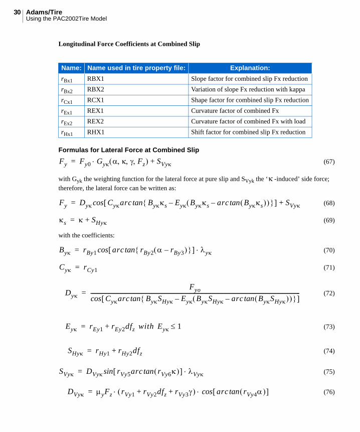
Longitudinal Force Coefficients at Combined Slip
Formulas for Lateral Force at Combined Slip
(67)
with Gyk the weighting function for the lateral force at pure slip and SVyk the ‘ -induced’ side force;
therefore, the lateral force can be written as:
(68)
(69)
with the coefficients:
(70)
(71)
(72)
(73)
(74)
(75)
(76)
Name: Name used in tire property file: Explanation:
rBx1 RBX1 Slope factor for combined slip Fx reduction
rBx2 RBX2 Variation of slope Fx reduction with kappa
rCx1 RCX1 Shape factor for combined slip Fx reduction
rEx1 REX1 Curvature factor of combined Fx
rEx2 REX2 Curvature factor of combined Fx with load
rHx1 RHX1 Shift factor for combined slip Fx reduction
Fy Fy0 Gy Fz SVy+=
Fy Dy Cyarc Bys Ey Bys arc Bys tan– – tan SVy+cos=
s SHy+=
By rBy1 arc rBy2 rBy3– tan ycos=
Cy rCy1=
DyFyo
Cyarc BySHy Ey BySHy arc BySHy tan– – tan cos-------------------------------------------------------------------------------------------------------------------------------------------------------------=
Ey rEy1 rEy2dfz with Ey 1+=
SHy rHy1 rHy2dfz+=
SVy DVy rVy5arc rVy6 tan Vysin=
DVy yFz rVy1 rVy2dfz rVy3+ + arc rVy4 tan cos =

31Using the PAC2002Tire Model
The weighting function appears is defined as:
(77)
Lateral Force Coefficients at Combined Slip
Formulas for Aligning Moment at Combined Slip
(78)
with:
(79)
(80)
(81)
(82)
Name: Name used in tire property file: Explanation:
rBy1 RBY1 Slope factor for combined Fy reduction
rBy2 RBY2 Variation of slope Fy reduction with alpha
rBy3 RBY3 Shift term for alpha in slope Fy reduction
rCy1 RCY1 Shape factor for combined Fy reduction
rEy1 REY1 Curvature factor of combined Fy
rEy2 REY2 Curvature factor of combined Fy with load
rHy1 RHY1 Shift factor for combined Fy reduction
rHy2 RHY2 Shift factor for combined Fy reduction with load
rVy1 RVY1 Kappa induced side force Svyk/Muy*Fz at Fznom
rVy2 RVY2 Variation of Svyk/Muy*Fz with load
rVy3 RVY3 Variation of Svyk/Muy*Fz with inclination
rVy4 RVY4 Variation of Svyk/Muy*Fz with alpha
rVy5 RVY5 Variation of Svyk/Muy*Fz with kappa
rVy6 RVY6 Variation of Svyk/Muy*Fz with atan (kappa)
GyCyarc Bys Ey Bys a– rc Bys tan – tan cos
Cyarc BySHy Ey BySHy a– rc BySHy tan – tan cos----------------------------------------------------------------------------------------------------------------------------------------------------------=
M
t Fy Mzr s Fx+ +–=
t t t eq =
Dt Ctarc Btt eq Et Btt eq arc Btt eq tan– – tan coscos=
Fy 0=
Fy SVy–=
Mzr Mzr r eq Dr arc Brr eq tan coscos= =
Adams/TireUsing the PAC2002Tire Model
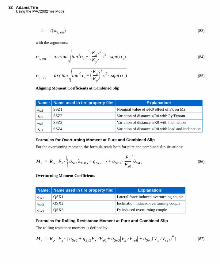
32
(83)
with the arguments:
(84)
(85)
Aligning Moment Coefficients at Combined Slip
Formulas for Overturning Moment at Pure and Combined Slip
For the overturning moment, the formula reads both for pure and combined slip situations:
(86)
Overturning Moment Coefficients
Formulas for Rolling Resistance Moment at Pure and Combined Slip
The rolling resistance moment is defined by:
(87)
Name: Name used in tire property file: Explanation:
ssz1 SSZ1 Nominal value of s/R0 effect of Fx on Mz
ssz2 SSZ2 Variation of distance s/R0 with Fy/Fznom
ssz3 SSZ3 Variation of distance s/R0 with inclination
ssz4 SSZ4 Variation of distance s/R0 with load and inclination
Name: Name used in tire property file: Explanation:
qsx1 QSX1 Lateral force induced overturning couple
qsx2 QSX2 Inclination induced overturning couple
qsx3 QSX3 Fy induced overturning couple
t t t eq =
t eq arc 2t
Kx
Ky------
22 t sgn+tantan=
r eq arc 2r
Kx
Ky------
22 r sgn+tantan=
Mx Ro Fz qSx1VMx qSx2 qSx3
Fy
Fz0--------+–
Mx =
My Ro Fz qSy1 qSy3Fx Fz0 qSy3 Vx Vref qSy4 Vx Vref 4+ + + =
33Using the PAC2002Tire Model
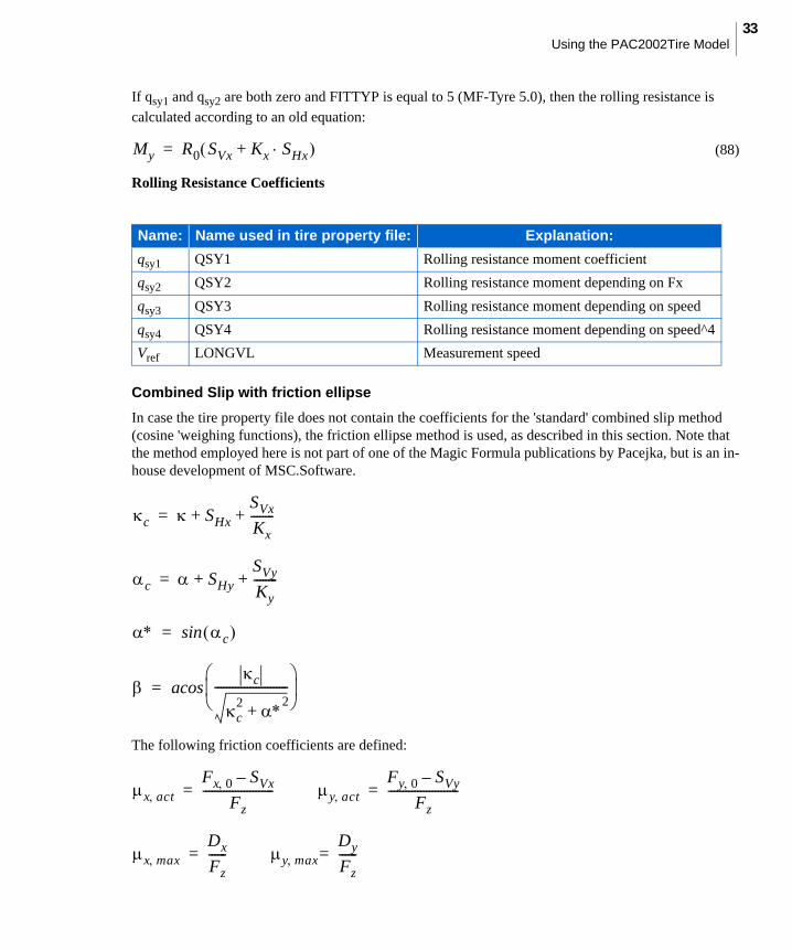
If qsy1 and qsy2 are both zero and FITTYP is equal to 5 (MF-Tyre 5.0), then the rolling resistance is
calculated according to an old equation:
(88)
Rolling Resistance Coefficients
Combined Slip with friction ellipse
In case the tire property file does not contain the coefficients for the 'standard' combined slip method (cosine 'weighing functions), the friction ellipse method is used, as described in this section. Note that the method employed here is not part of one of the Magic Formula publications by Pacejka, but is an in-house development of MSC.Software.
The following friction coefficients are defined:
Name: Name used in tire property file: Explanation:
qsy1 QSY1 Rolling resistance moment coefficient
qsy2 QSY2 Rolling resistance moment depending on Fx
qsy3 QSY3 Rolling resistance moment depending on speed
qsy4 QSY4 Rolling resistance moment depending on speed^4
Vref LONGVL Measurement speed
My R0 SVx Kx SHx+ =
c SHx
SVx
Kx--------+ +=
c SHy
SVy
Ky--------+ +=
c sin=
c
c2
2+
-------------------------
acos=
x actFx 0 SVx–
Fz------------------------= y act
Fy 0 SVy–
Fz------------------------=
x maxDx
Fz------= y max
Dy
Fz------=
Adams/TireUsing the PAC2002Tire Model
34
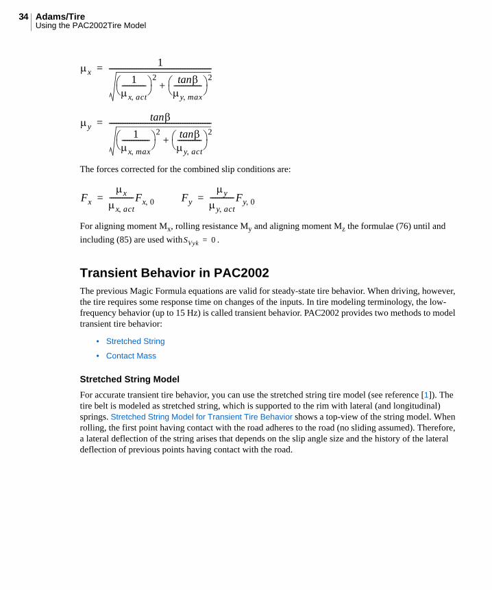
The forces corrected for the combined slip conditions are:
For aligning moment Mx, rolling resistance My and aligning moment Mz the formulae (76) until and
including (85) are used with .
Transient Behavior in PAC2002The previous Magic Formula equations are valid for steady-state tire behavior. When driving, however, the tire requires some response time on changes of the inputs. In tire modeling terminology, the low-frequency behavior (up to 15 Hz) is called transient behavior. PAC2002 provides two methods to model transient tire behavior:
• Stretched String
• Contact Mass
Stretched String Model
For accurate transient tire behavior, you can use the stretched string tire model (see reference [1]). The tire belt is modeled as stretched string, which is supported to the rim with lateral (and longitudinal) springs. Stretched String Model for Transient Tire Behavior shows a top-view of the string model. When rolling, the first point having contact with the road adheres to the road (no sliding assumed). Therefore, a lateral deflection of the string arises that depends on the slip angle size and the history of the lateral deflection of previous points having contact with the road.
x1
1x act------------- 2 tan
y max--------------- 2
+
--------------------------------------------------------=
ytan
1x max--------------- 2 tan
y act------------- 2
+
--------------------------------------------------------=
Fx
x
x act-------------Fx 0= Fy
y
y act-------------Fy 0=
SVyk 0=
35Using the PAC2002Tire Model
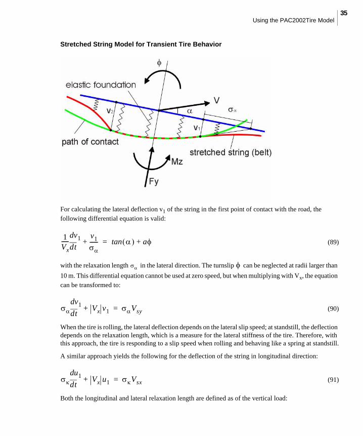
Stretched String Model for Transient Tire Behavior
For calculating the lateral deflection v1 of the string in the first point of contact with the road, the
following differential equation is valid:
(89)
with the relaxation length in the lateral direction. The turnslip can be neglected at radii larger than
10 m. This differential equation cannot be used at zero speed, but when multiplying with Vx, the equation
can be transformed to:
(90)
When the tire is rolling, the lateral deflection depends on the lateral slip speed; at standstill, the deflection depends on the relaxation length, which is a measure for the lateral stiffness of the tire. Therefore, with this approach, the tire is responding to a slip speed when rolling and behaving like a spring at standstill.
A similar approach yields the following for the deflection of the string in longitudinal direction:
(91)
Both the longitudinal and lateral relaxation length are defined as of the vertical load:
1Vx-----
td
dv1 v1
------+ a+tan=
td
dv1 Vx v1+ Vsy=
td
du1 Vx u1+ Vsx=
Adams/TireUsing the PAC2002Tire Model
36
(92)
(93)
Now the practical slip quantities, and , are defined based on the tire deformation:
(94)
(95)
Using these practical slip quantities, and , the Magic Formula equations can be used to calculate the tire-road interaction forces and moments:
(96)
(97)
(98)
(99)
Coefficients and Transient Response
Name:Name used in tire
property file: Explanation:
pTx1 PTX1 Longitudinal relaxation length at Fznom
pTx2 PTX2 Variation of longitudinal relaxation length with load
pTx3 PTX3 Variation of longitudinal relaxation length with exponent of load
pTy1 PTY1 Peak value of relaxation length for lateral direction
pTy2 PTY2 Shape factor for lateral relaxation length
qTz1 QTZ1 Gyroscopic moment constant
Mbelt MBELT Belt mass of the wheel
Fz pTx1 pTx2dfz+ pTx3dfz R0 Fz0 exp =
pTy1 2arcFz
pTy2Fz0Fz0 ---------------------------------
tan 1 pKy3 y– R0Fz0 sin=
'u1
x----- Vx sin=
'v1
------ atan=
Fx Fx ' ' Fz =
Fy Fy ' ' Fz =
M'z M'z ' ' Fz =
Mz
Mz ' ' Fz =
37Using the PAC2002Tire Model
Contact Mass Model
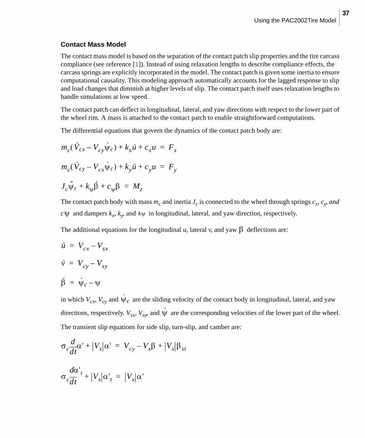
The contact mass model is based on the separation of the contact patch slip properties and the tire carcass compliance (see reference [1]). Instead of using relaxation lengths to describe compliance effects, the carcass springs are explicitly incorporated in the model. The contact patch is given some inertia to ensure computational causality. This modeling approach automatically accounts for the lagged response to slip and load changes that diminish at higher levels of slip. The contact patch itself uses relaxation lengths to handle simulations at low speed.
The contact patch can deflect in longitudinal, lateral, and yaw directions with respect to the lower part of the wheel rim. A mass is attached to the contact patch to enable straightforward computations.
The differential equations that govern the dynamics of the contact patch body are:
The contact patch body with mass mc and inertia Jc is connected to the wheel through springs cx, cy, and
c and dampers kx, ky, and in longitudinal, lateral, and yaw direction, respectively.
The additional equations for the longitudinal u, lateral v, and yaw deflections are:
in which Vcx, Vcy and are the sliding velocity of the contact body in longitudinal, lateral, and yaw
directions, respectively. Vsx, Vsy, and are the corresponding velocities of the lower part of the wheel.
The transient slip equations for side slip, turn-slip, and camber are:
mc V· cx Vcy·
c– kxu· cxu+ + Fx=
mc V· cy Vcx·
c– kyu· cyu+ + Fy=
Jc··
c k· c+ + Mz=
k
u· Vcx Vsx–=
v· Vcy Vsy–=
· · c –=
· c
·
c tdd ' Vx '+ Vcy Vx– Vx st+=
c td
d't Vx 't+ Vx '=
Adams/TireUsing the PAC2002Tire Model
38
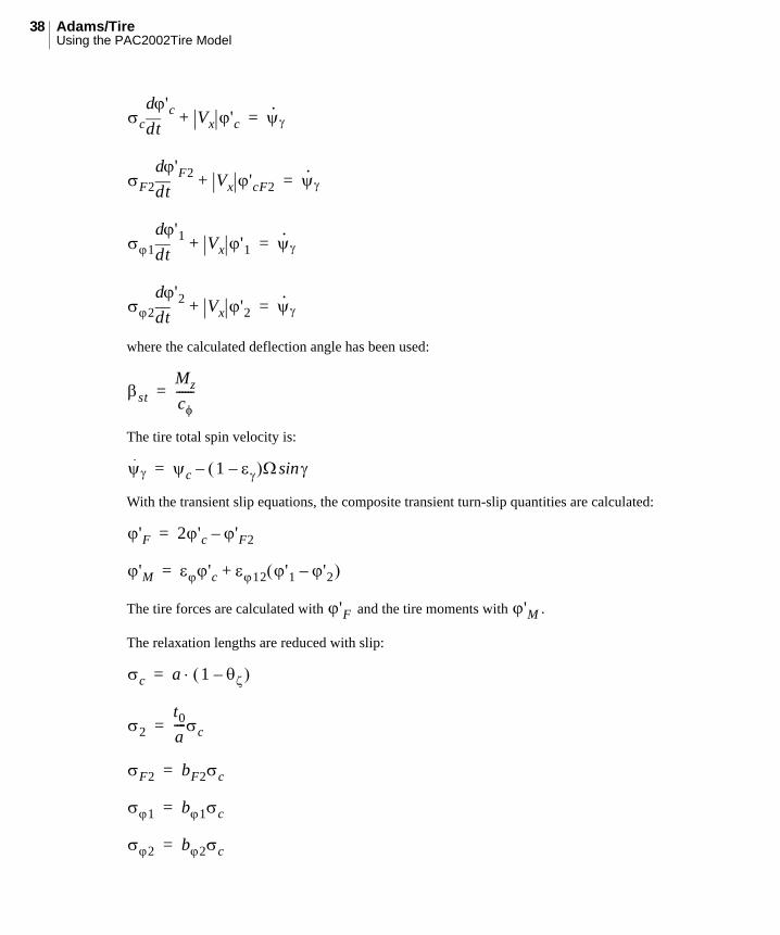
where the calculated deflection angle has been used:
The tire total spin velocity is:
With the transient slip equations, the composite transient turn-slip quantities are calculated:
The tire forces are calculated with and the tire moments with .
The relaxation lengths are reduced with slip:
c td
d'c Vx 'c+ · =
F2 td
d'F2 Vx 'cF2+ · =
1 td
d'1 Vx '1+ · =
2 td
d'2 Vx '2+ · =
stMz
c------=
· c 1 – sin–=
'F 2'c 'F2–=
'M 'c 12 '1 '2– +=
'F 'M
c a 1 – =
2
t0
a----c=
F2 bF2c=
1 b1c=
2 b2c=
39Using the PAC2002Tire Model
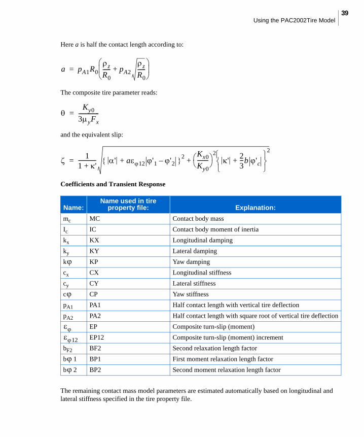
Here a is half the contact length according to:
The composite tire parameter reads:
and the equivalent slip:
Coefficients and Transient Response
The remaining contact mass model parameters are estimated automatically based on longitudinal and lateral stiffness specified in the tire property file.
Name:Name used in tire
property file: Explanation:
mc MC Contact body mass
Ic IC Contact body moment of inertia
kx KX Longitudinal damping
ky KY Lateral damping
k KP Yaw damping
cx CX Longitudinal stiffness
cy CY Lateral stiffness
c CP Yaw stiffness
pA1 PA1 Half contact length with vertical tire deflection
pA2 PA2 Half contact length with square root of vertical tire deflection
EP Composite turn-slip (moment)
EP12 Composite turn-slip (moment) increment
bF2 BF2 Second relaxation length factor
b 1 BP1 First moment relaxation length factor
b 2 BP2 Second moment relaxation length factor
a pA1R0z
R0------ pA2
z
R0------+
=
Ky0
3yFx---------------=
11 '+------------- ' a12 '1 '2–+ 2 Kx0
Ky0--------
2'
23---b 'c+
2
+=
12
Adams/TireUsing the PAC2002Tire Model
40
Gyroscopic Couple in PAC2002When having fast rotations about the vertical axis in the wheel plane, the inertia of the tire belt may lead to gyroscopic effects. To cope with this additional moment, the following contribution is added to the total aligning moment:
(100)
with the parameter (in addition to the basic tire parameter mbelt):
(101)
and:
(102)
The total aligning moment now becomes:
(103)
Coefficients and Transient Response
Left and Right Side TiresIn general, a tire produces a lateral force and aligning moment at zero slip angle due to the tire construction, known as conicity and plysteer. In addition, the tire characteristics cannot be symmetric for positive and negative slip angles.
A tire property file with the parameters for the model results from testing with a tire that is mounted in a tire test bench comparable either to the left or the right side of a vehicle. If these coefficients are used for both the left and the right side of the vehicle model, the vehicle does not drive straight at zero steering wheel angle.
Name:Name used in
tire property file: Explanation:
pTx1 PTX1 Longitudinal relaxation length at Fznom
pTx2 PTX2 Variation of longitudinal relaxation length with load
pTx3 PTX3 Variation of longitudinal relaxation length with exponent of load
pTy1 PTY1 Peak value of relaxation length for lateral direction
pTy2 PTY2 Shape factor for lateral relaxation length
qTz1 QTZ1 Gyroscopic moment constant
Mbelt MBELT Belt mass of the wheel
Mz gyr cgyrmbeltVrl tddv
arc Brr eq tan cos=
cgyr qTz1 gyr=
arc Brr eq tan cos 1=
Mz M'z Mz gyr+=

41Using the PAC2002Tire Model
The latest versions of tire property files contain a keyword TYRESIDE in the [MODEL] section that indicates for which side of the vehicle the tire parameters in that file are valid (TYRESIDE = 'LEFT' or TYRESIDE = 'RIGHT'). .
If this keyword is available, Adams/Car corrects for the conicity and plysteer and asymmetry when using a tire property file on the opposite side of the vehicle. In fact, the tire characteristics are mirrored with respect to slip angle zero. In Adams/View, this option can only be used when the tire is generated by the graphical user interface: select Build -> Forces -> Special Force: Tire.
Next to the LEFT and RIGHT side option of TYRESIDE, you can also set SYMMETRIC: then the tire characteristics are modified during initialization to show symmetric performance for left and right side corners and zero conicity and plysteer (no offsets).Also, when you set the tire property file to SYMMETRIC, the tire characteristics are changed to symmetric behavior.
Adams/TireUsing the PAC2002Tire Model
42
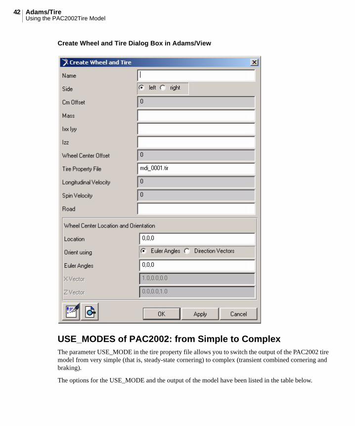
Create Wheel and Tire Dialog Box in Adams/View
USE_MODES of PAC2002: from Simple to ComplexThe parameter USE_MODE in the tire property file allows you to switch the output of the PAC2002 tire model from very simple (that is, steady-state cornering) to complex (transient combined cornering and braking).
The options for the USE_MODE and the output of the model have been listed in the table below.
43Using the PAC2002Tire Model
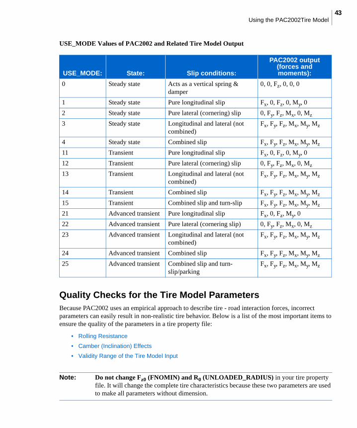
USE_MODE Values of PAC2002 and Related Tire Model Output
Quality Checks for the Tire Model ParametersBecause PAC2002 uses an empirical approach to describe tire - road interaction forces, incorrect parameters can easily result in non-realistic tire behavior. Below is a list of the most important items to ensure the quality of the parameters in a tire property file:
• Rolling Resistance
• Camber (Inclination) Effects
• Validity Range of the Tire Model Input
USE_MODE: State: Slip conditions:
PAC2002 output(forces and moments):
0 Steady state Acts as a vertical spring & damper
0, 0, Fz, 0, 0, 0
1 Steady state Pure longitudinal slip Fx, 0, Fz, 0, My, 0
2 Steady state Pure lateral (cornering) slip 0, Fy, Fz, Mx, 0, Mz
3 Steady state Longitudinal and lateral (not combined)
Fx, Fy, Fz, Mx, My, Mz
4 Steady state Combined slip Fx, Fy, Fz, Mx, My, Mz
11 Transient Pure longitudinal slip Fx, 0, Fz, 0, My, 0
12 Transient Pure lateral (cornering) slip 0, Fy, Fz, Mx, 0, Mz
13 Transient Longitudinal and lateral (not combined)
Fx, Fy, Fz, Mx, My, Mz
14 Transient Combined slip Fx, Fy, Fz, Mx, My, Mz
15 Transient Combined slip and turn-slip Fx, Fy, Fz, Mx, My, Mz
21 Advanced transient Pure longitudinal slip Fx, 0, Fz, My, 0
22 Advanced transient Pure lateral (cornering slip) 0, Fy, Fz, Mx, 0, Mz
23 Advanced transient Longitudinal and lateral (not combined)
Fx, Fy, Fz, Mx, My, Mz
24 Advanced transient Combined slip Fx, Fy, Fz, Mx, My, Mz
25 Advanced transient Combined slip and turn-slip/parking
Fx, Fy, Fz, Mx, My, Mz
Note: Do not change Fz0 (FNOMIN) and R0 (UNLOADED_RADIUS) in your tire property file. It will change the complete tire characteristics because these two parameters are used to make all parameters without dimension.
Adams/TireUsing the PAC2002Tire Model
44
Rolling Resistance
For a realistic rolling resistance, the parameter qsy1 must be positive. For car tires, it can be in the order
of 0.006 - 0.01 (0.6% - 1.0%); for heavy commercial truck tires, it can be around 0.006 (0.6%).
Tire property files with the keyword FITTYP=5 determine the rolling resistance in a different way (see equation (88)). To avoid the ‘old’ rolling resistance calculation, remove the keyword FITTYP and add a section like the following:
$---------------------------------------------------rolling resistance[ROLLING_COEFFICIENTS]QSY1 = 0.01QSY2 = 0QSY3 = 0QSY4 = 0
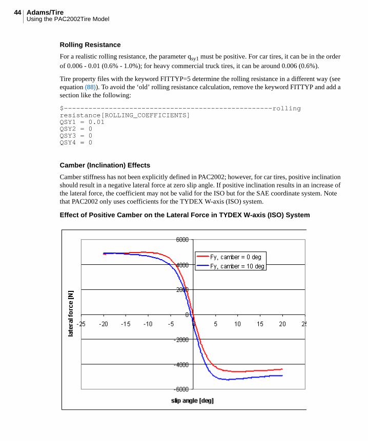
Camber (Inclination) Effects
Camber stiffness has not been explicitly defined in PAC2002; however, for car tires, positive inclination should result in a negative lateral force at zero slip angle. If positive inclination results in an increase of the lateral force, the coefficient may not be valid for the ISO but for the SAE coordinate system. Note that PAC2002 only uses coefficients for the TYDEX W-axis (ISO) system.
Effect of Positive Camber on the Lateral Force in TYDEX W-axis (ISO) System

45Using the PAC2002Tire Model
The table below lists further checks on the PAC2002 parameters.
Checklist for PAC2002 Parameters and Properties
Validity Range of the Tire Model Input
In the tire property file, a range of the input variables has been given in which the tire properties are supposed to be valid. These validity range parameters are (the listed values can be different):
$--------------------------------------------------long_slip_range[LONG_SLIP_RANGE]KPUMIN = -1.5 $Minimum valid wheel slip KPUMAX = 1.5 $Maximum valid wheel slip $-------------------------------------------------slip_angle_range[SLIP_ANGLE_RANGE]ALPMIN = -1.5708 $Minimum valid slip angle ALPMAX = 1.5708 $Maximum valid slip angle $--------------------------------------------inclination_slip_range[INCLINATION_ANGLE_RANGE]CAMMIN = -0.26181 $Minimum valid camber angle CAMMAX = 0.26181 $Maximum valid camber angle $----------------------------------------------vertical_force_range[VERTICAL_FORCE_RANGE]FZMIN = 225 $Minimum allowed wheel load FZMAX = 10125 $Maximum allowed wheel load
If one of the input parameters exceeds a minimum or maximum validity value, the calculation in the tire model is performed with the minimum or maximum value of this range to avoid non-realistic tire behavior. In that case, a message appears warning you that one of the inputs exceeds a validity value.
Parameter/property: Requirement: Explanation:
LONGVL 1 m/s Reference velocity at which parameters are measured
VXLOW Approximately 1 m/s Threshold for scaling down forces and moments
Dx > 0 Peak friction (see equation (22))
pDx1/pDx2 < 0 Peak friction Fx must decrease with increasing load
Kx > 0 Long slip stiffness (see equation (25))
Dy > 0 Peak friction (see equation (34))
pDy1/pDy2 < 0 Peak friction Fx must decrease with increasing load
Ky < 0 Cornering stiffness (see equation (37))
qsy1 > 0 Rolling resistance, in the range of 0.005 - 0.015
Adams/TireUsing the PAC2002Tire Model
46
Standard Tire Interface (STI) for PAC2002Because all Adams products use the Standard Tire Interface (STI) for linking the tire models to Adams/Solver, below is a brief background of the STI history (see also reference [4]).
At the First International Colloquium on Tire Models for Vehicle Dynamics Analysis on October 21-22, 1991, the International Tire Workshop working group was established (TYDEX).
The working group concentrated on tire measurements and tire models used for vehicle simulation purposes. For most vehicle dynamics studies, people used to develop their own tire models. Because all car manufacturers and their tire suppliers have the same goal (that is, development of tires to improve dynamic safety of the vehicle) it aimed for standardization in tire behavior description.
In TYDEX, two expert groups, consisting of participants of vehicle industry (passenger cars and trucks), tire manufacturers, other suppliers and research laboratories, had been defined with following goals:
• The first expert group's (Tire Measurements - Tire Modeling) main goal was to specify an interface between tire measurements and tire models. The result was the TYDEX-Format [2] to describe tire measurement data.
• The second expert group's (Tire Modeling - Vehicle Modeling) main goal was to specify an interface between tire models and simulation tools, which resulted in the Standard Tire Interface (STI) [3]. The use of this interface should ensure that a wide range of simulation software can be linked to a wide range of tire modeling software.
Definitions• General
• Tire Kinematics
• Slip Quantities
• Force and Moments
General
General Definitions
Term: Definition:
Road tangent plane Plane with the normal unit vector (tangent to the road) in the tire-road contact point C.
C-axis system Coordinate system mounted on the wheel carrier at the wheel center according to TYDEX, ISO orientation.
Wheel plane The plane in the wheel center that is formed by the wheel when considered a rigid disc with zero width.

47Using the PAC2002Tire Model
Tire Kinematics
Tire Kinematics Definitions
Slip Quantities
Slip Quantities Definitions
Contact point C Contact point between tire and road, defined as the intersection of the wheel plane and the projection of the wheel axis onto the road plane.
W-axis system Coordinate system at the tire contact point C, according to TYDEX, ISO orientation.
Parameter: Definition: Units:
R0 Unloaded tire radius [m]
R Loaded tire radius [m]
Re Effective tire radius [m]
Radial tire deflection [m]
Dimensionless radial tire deflection [-]
Radial tire deflection at nominal load [m]
mbelt Tire belt mass [kg]
Rotational velocity of the wheel [rads-1]
Parameter: Definition: Units:
V Vehicle speed [ms-1]
Vsx Slip speed in x direction [ms-1]
Vsy Slip speed in y direction [ms-1]
Vs Resulting slip speed [ms-1]
Vx Rolling speed in x direction [ms-1]
Vy Lateral speed of tire contact center [ms-1]
Vr Linear speed of rolling [ms-1]
Longitudinal slip [-]
Slip angle [rad]
Inclination angle [rad]
Term: Definition:
d
FZ0

Adams/TireUsing the PAC2002Tire Model
48
Forces and Moments
Force and Moment Definitions
References1. H.B. Pacejka, Tyre and Vehicle Dynamics, 2002, Butterworth-Heinemann, ISBN 0 7506 5141 5.
2. H.-J. Unrau, J. Zamow, TYDEX-Format, Description and Reference Manual, Release 1.1, Initiated by the International Tire Working Group, July 1995.
3. A. Riedel, Standard Tire Interface, Release 1.2, Initiated by the Tire Workgroup, June 1995.
4. J.J.M. van Oosten, H.-J. Unrau, G. Riedel, E. Bakker, TYDEX Workshop: Standardisation of Data Exchange in Tyre Testing and Tyre Modelling, Proceedings of the 2nd International Colloquium on Tyre Models for Vehicle Dynamics Analysis, Vehicle System Dynamics, Volume 27, Swets & Zeitlinger, Amsterdam/Lisse, 1996.
Example of PAC2002 Tire Property File[MDI_HEADER]FILE_TYPE ='tir'FILE_VERSION =3.0FILE_FORMAT ='ASCII'! : TIRE_VERSION : PAC2002! : COMMENT : Tire 235/60R16! : COMMENT : Manufacturer ! : COMMENT : Nom. section with (m) 0.235 ! : COMMENT : Nom. aspect ratio (-) 60! : COMMENT : Infl. pressure (Pa) 200000! : COMMENT : Rim radius (m) 0.19 ! : COMMENT : Measurement ID ! : COMMENT : Test speed (m/s) 16.6 ! : COMMENT : Road surface ! : COMMENT : Road condition Dry! : FILE_FORMAT : ASCII! : Copyright MSC.Software, Fri Jan 23 14:30:06 2004!! USE_MODE specifies the type of calculation performed:! 0: Fz only, no Magic Formula evaluation
Abbreviation: Definition: Units:
Fz Vertical wheel load [N]
Fz0 Nominal load [N]
dfz Dimensionless vertical load [-]
Fx Longitudinal force [N]
Fy Lateral force [N]
Mx Overturning moment [Nm]
My Braking/driving moment [Nm]
Mz Aligning moment [Nm]
49Using the PAC2002Tire Model
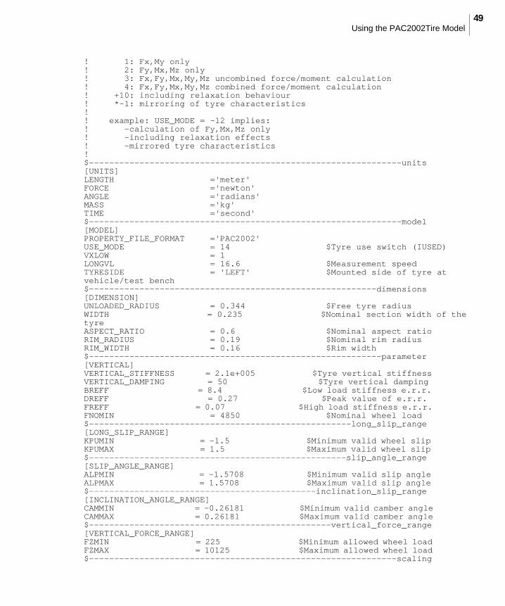
! 1: Fx,My only! 2: Fy,Mx,Mz only! 3: Fx,Fy,Mx,My,Mz uncombined force/moment calculation! 4: Fx,Fy,Mx,My,Mz combined force/moment calculation! +10: including relaxation behaviour! *-1: mirroring of tyre characteristics!! example: USE_MODE = -12 implies:! -calculation of Fy,Mx,Mz only! -including relaxation effects! -mirrored tyre characteristics!$--------------------------------------------------------------units[UNITS]LENGTH ='meter'FORCE ='newton'ANGLE ='radians'MASS ='kg'TIME ='second'$--------------------------------------------------------------model[MODEL]PROPERTY_FILE_FORMAT ='PAC2002'USE_MODE = 14 $Tyre use switch (IUSED)VXLOW = 1 LONGVL = 16.6 $Measurement speed TYRESIDE = 'LEFT' $Mounted side of tyre at vehicle/test bench$---------------------------------------------------------dimensions[DIMENSION]UNLOADED_RADIUS = 0.344 $Free tyre radius WIDTH = 0.235 $Nominal section width of the tyre ASPECT_RATIO = 0.6 $Nominal aspect ratioRIM_RADIUS = 0.19 $Nominal rim radius RIM_WIDTH = 0.16 $Rim width $----------------------------------------------------------parameter[VERTICAL]VERTICAL_STIFFNESS = 2.1e+005 $Tyre vertical stiffness VERTICAL_DAMPING = 50 $Tyre vertical damping BREFF = 8.4 $Low load stiffness e.r.r. DREFF = 0.27 $Peak value of e.r.r. FREFF = 0.07 $High load stiffness e.r.r. FNOMIN = 4850 $Nominal wheel load$----------------------------------------------------long_slip_range[LONG_SLIP_RANGE]KPUMIN = -1.5 $Minimum valid wheel slip KPUMAX = 1.5 $Maximum valid wheel slip $---------------------------------------------------slip_angle_range[SLIP_ANGLE_RANGE]ALPMIN = -1.5708 $Minimum valid slip angle ALPMAX = 1.5708 $Maximum valid slip angle $---------------------------------------------inclination_slip_range[INCLINATION_ANGLE_RANGE]CAMMIN = -0.26181 $Minimum valid camber angle CAMMAX = 0.26181 $Maximum valid camber angle $------------------------------------------------vertical_force_range[VERTICAL_FORCE_RANGE]FZMIN = 225 $Minimum allowed wheel load FZMAX = 10125 $Maximum allowed wheel load $-------------------------------------------------------------scaling

Adams/TireUsing the PAC2002Tire Model
50
[SCALING_COEFFICIENTS]LFZO = 1 $Scale factor of nominal (rated) load LCX = 1 $Scale factor of Fx shape factorLMUX = 1 $Scale factor of Fx peak friction coefficientLEX = 1 $Scale factor of Fx curvature factorLKX = 1 $Scale factor of Fx slip stiffnessLHX = 1 $Scale factor of Fx horizontal shift LVX = 1 $Scale factor of Fx vertical shiftLGAX = 1 $Scale factor of camber for FxLCY = 1 $Scale factor of Fy shape factorLMUY = 1 $Scale factor of Fy peak friction coefficientLEY = 1 $Scale factor of Fy curvature factorLKY = 1 $Scale factor of Fy cornering stiffnessLHY = 1 $Scale factor of Fy horizontal shiftLVY = 1 $Scale factor of Fy vertical shiftLGAY = 1 $Scale factor of camber for FyLTR = 1 $Scale factor of Peak of pneumatic trailLRES = 1 $Scale factor for offset of residual torqueLGAZ = 1 $Scale factor of camber for MzLXAL = 1 $Scale factor of alpha influence on FxLYKA = 1 $Scale factor of alpha influence on FxLVYKA = 1 $Scale factor of kappa induced FyLS = 1 $Scale factor of Moment arm of FxLSGKP = 1 $Scale factor of Relaxation length of FxLSGAL = 1 $Scale factor of Relaxation length of FyLGYR = 1 $Scale factor of gyroscopic torqueLMX = 1 $Scale factor of overturning coupleLVMX = 1 $Scale factor of Mx vertical shiftLMY = 1 $Scale factor of rolling resistance torque $-------------------------------------------------------longitudinal[LONGITUDINAL_COEFFICIENTS]PCX1 = 1.6411 $Shape factor Cfx for longitudinal force PDX1 = 1.1739 $Longitudinal friction Mux at Fznom PDX2 = -0.16395 $Variation of friction Mux with load PDX3 = 0 $Variation of friction Mux with camber PEX1 = 0.46403 $Longitudinal curvature Efx at Fznom PEX2 = 0.25022 $Variation of curvature Efx with load PEX3 = 0.067842 $Variation of curvature Efx with load squared PEX4 = -3.7604e-005 $Factor in curvature Efx while driving PKX1 = 22.303 $Longitudinal slip stiffness Kfx/Fz at Fznom PKX2 = 0.48896 $Variation of slip stiffness Kfx/Fz with load PKX3 = 0.21253 $Exponent in slip stiffness Kfx/Fz with load PHX1 = 0.0012297 $Horizontal shift Shx at Fznom PHX2 = 0.0004318 $Variation of shift Shx with load PVX1 = -8.8098e-006 $Vertical shift Svx/Fz at Fznom PVX2 = 1.862e-005 $Variation of shift Svx/Fz with load RBX1 = 13.276 $Slope factor for combined slip Fx reduction RBX2 = -13.778 $Variation of slope Fx reduction with kappa RCX1 = 1.2568 $Shape factor for combined slip Fx reduction REX1 = 0.65225 $Curvature factor of combined Fx REX2 = -0.24948 $Curvature factor of combined Fx with load RHX1 = 0.0050722 $Shift factor for combined slip Fx reduction PTX1 = 2.3657 $Relaxation length SigKap0/Fz at Fznom PTX2 = 1.4112 $Variation of SigKap0/Fz with load PTX3 = 0.56626 $Variation of SigKap0/Fz with exponent of load $--------------------------------------------------------overturning[OVERTURNING_COEFFICIENTS]QSX1 = 0 $Lateral force induced overturning moment QSX2 = 0 $Camber induced overturning couple QSX3 = 0 $Fy induced overturning couple
51Using the PAC2002Tire Model
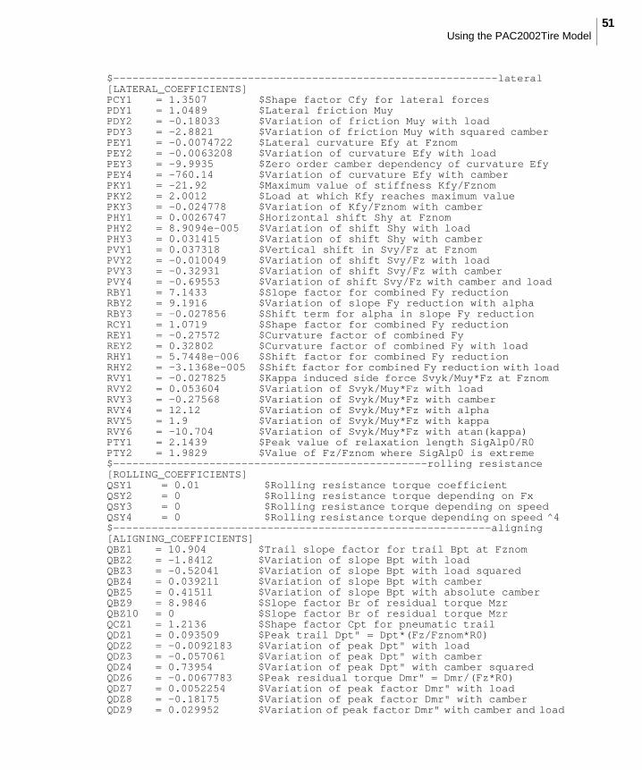
$------------------------------------------------------------lateral[LATERAL_COEFFICIENTS]PCY1 = 1.3507 $Shape factor Cfy for lateral forces PDY1 = 1.0489 $Lateral friction Muy PDY2 = -0.18033 $Variation of friction Muy with load PDY3 = -2.8821 $Variation of friction Muy with squared camber PEY1 = -0.0074722 $Lateral curvature Efy at Fznom PEY2 = -0.0063208 $Variation of curvature Efy with load PEY3 = -9.9935 $Zero order camber dependency of curvature Efy PEY4 = -760.14 $Variation of curvature Efy with camber PKY1 = -21.92 $Maximum value of stiffness Kfy/Fznom PKY2 = 2.0012 $Load at which Kfy reaches maximum value PKY3 = -0.024778 $Variation of Kfy/Fznom with camber PHY1 = 0.0026747 $Horizontal shift Shy at Fznom PHY2 = 8.9094e-005 $Variation of shift Shy with load PHY3 = 0.031415 $Variation of shift Shy with camber PVY1 = 0.037318 $Vertical shift in Svy/Fz at Fznom PVY2 = -0.010049 $Variation of shift Svy/Fz with load PVY3 = -0.32931 $Variation of shift Svy/Fz with camber PVY4 = -0.69553 $Variation of shift Svy/Fz with camber and load RBY1 = 7.1433 $Slope factor for combined Fy reduction RBY2 = 9.1916 $Variation of slope Fy reduction with alpha RBY3 = -0.027856 $Shift term for alpha in slope Fy reduction RCY1 = 1.0719 $Shape factor for combined Fy reduction REY1 = -0.27572 $Curvature factor of combined Fy REY2 = 0.32802 $Curvature factor of combined Fy with load RHY1 = 5.7448e-006 $Shift factor for combined Fy reduction RHY2 = -3.1368e-005 $Shift factor for combined Fy reduction with load RVY1 = -0.027825 $Kappa induced side force Svyk/Muy*Fz at Fznom RVY2 = 0.053604 $Variation of Svyk/Muy*Fz with load RVY3 = -0.27568 $Variation of Svyk/Muy*Fz with camber RVY4 = 12.12 $Variation of Svyk/Muy*Fz with alpha RVY5 = 1.9 $Variation of Svyk/Muy*Fz with kappa RVY6 = -10.704 $Variation of Svyk/Muy*Fz with atan(kappa) PTY1 = 2.1439 $Peak value of relaxation length SigAlp0/R0 PTY2 = 1.9829 $Value of Fz/Fznom where SigAlp0 is extreme $-------------------------------------------------rolling resistance[ROLLING_COEFFICIENTS]QSY1 = 0.01 $Rolling resistance torque coefficient QSY2 = 0 $Rolling resistance torque depending on Fx QSY3 = 0 $Rolling resistance torque depending on speed QSY4 = 0 $Rolling resistance torque depending on speed ̂ 4 $-----------------------------------------------------------aligning[ALIGNING_COEFFICIENTS]QBZ1 = 10.904 $Trail slope factor for trail Bpt at Fznom QBZ2 = -1.8412 $Variation of slope Bpt with load QBZ3 = -0.52041 $Variation of slope Bpt with load squared QBZ4 = 0.039211 $Variation of slope Bpt with camber QBZ5 = 0.41511 $Variation of slope Bpt with absolute camber QBZ9 = 8.9846 $Slope factor Br of residual torque Mzr QBZ10 = 0 $Slope factor Br of residual torque Mzr QCZ1 = 1.2136 $Shape factor Cpt for pneumatic trail QDZ1 = 0.093509 $Peak trail Dpt" = Dpt*(Fz/Fznom*R0) QDZ2 = -0.0092183 $Variation of peak Dpt" with load QDZ3 = -0.057061 $Variation of peak Dpt" with camber QDZ4 = 0.73954 $Variation of peak Dpt" with camber squared QDZ6 = -0.0067783 $Peak residual torque Dmr" = Dmr/(Fz*R0) QDZ7 = 0.0052254 $Variation of peak factor Dmr" with load QDZ8 = -0.18175 $Variation of peak factor Dmr" with camber QDZ9 = 0.029952 $Variation of peak factor Dmr" with camber and load
Adams/TireUsing the PAC2002Tire Model
52
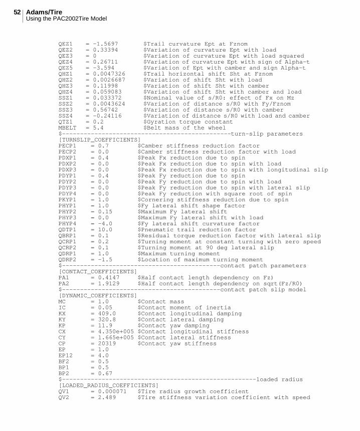
QEZ1 = -1.5697 $Trail curvature Ept at Fznom QEZ2 = 0.33394 $Variation of curvature Ept with load QEZ3 = 0 $Variation of curvature Ept with load squared QEZ4 = 0.26711 $Variation of curvature Ept with sign of Alpha-t QEZ5 = -3.594 $Variation of Ept with camber and sign Alpha-t QHZ1 = 0.0047326 $Trail horizontal shift Sht at Fznom QHZ2 = 0.0026687 $Variation of shift Sht with load QHZ3 = 0.11998 $Variation of shift Sht with camber QHZ4 = 0.059083 $Variation of shift Sht with camber and load SSZ1 = 0.033372 $Nominal value of s/R0: effect of Fx on Mz SSZ2 = 0.0043624 $Variation of distance s/R0 with Fy/Fznom SSZ3 = 0.56742 $Variation of distance s/R0 with camber SSZ4 = -0.24116 $Variation of distance s/R0 with load and camber QTZ1 = 0.2 $Gyration torque constant MBELT = 5.4 $Belt mass of the wheel $-----------------------------------------------turn-slip parameters[TURNSLIP_COEFFICIENTS]PECP1 = 0.7 $Camber stiffness reduction factorPECP2 = 0.0 $Camber stiffness reduction factor with loadPDXP1 = 0.4 $Peak Fx reduction due to spinPDXP2 = 0.0 $Peak Fx reduction due to spin with loadPDXP3 = 0.0 $Peak Fx reduction due to spin with longitudinal slipPDYP1 = 0.4 $Peak Fy reduction due to spinPDYP2 = 0.0 $Peak Fy reduction due to spin with loadPDYP3 = 0.0 $Peak Fy reduction due to spin with lateral slipPDYP4 = 0.0 $Peak Fy reduction with square root of spinPKYP1 = 1.0 $Cornering stiffness reduction due to spinPHYP1 = 1.0 $Fy lateral shift shape factorPHYP2 = 0.15 $Maximum Fy lateral shiftPHYP3 = 0.0 $Maximum Fy lateral shift with loadPHYP4 = -4.0 $Fy lateral shift curvature factorQDTP1 = 10.0 $Pneumatic trail reduction factorQBRP1 = 0.1 $Residual torque reduction factor with lateral slipQCRP1 = 0.2 $Turning moment at constant turning with zero speedQCRP2 = 0.1 $Turning moment at 90 deg lateral slipQDRP1 = 1.0 $Maximum turning momentQDRP2 = -1.5 $Location of maximum turning moment$--------------------------------------------contact patch parameters[CONTACT_COEFFICIENTS]PA1 = 0.4147 $Half contact length dependency on Fz)PA2 = 1.9129 $Half contact length dependency on sqrt(Fz/R0)$--------------------------------------------contact patch slip model[DYNAMIC_COEFFICIENTS]MC = 1.0 $Contact massIC = 0.05 $Contact moment of inertiaKX = 409.0 $Contact longitudinal dampingKY = 320.8 $Contact lateral dampingKP = 11.9 $Contact yaw dampingCX = 4.350e+005 $Contact longitudinal stiffnessCY = 1.665e+005 $Contact lateral stiffnessCP = 20319 $Contact yaw stiffnessEP = 1.0EP12 = 4.0BF2 = 0.5BP1 = 0.5BP2 = 0.67$------------------------------------------------------loaded radius[LOADED_RADIUS_COEFFICIENTS]QV1 = 0.000071 $Tire radius growth coefficientQV2 = 2.489 $Tire stiffness variation coefficient with speed

53Using the PAC2002Tire Model
QFCX1 = 0.1 $Tire stiffness interaction with FxQFCY1 = 0.3 $Tire stiffness interaction with FyQFCG1 = 0.0 $Tire stiffness interaction with camberQFZ1 = 0.0 $Linear stiffness coefficient, if zero, VERTICAL_STIFFNESS is takenQFZ2 = 14.35 $Tire vertical stiffness coefficient (quadratic)
Contact MethodsThe PAC2002 model supports the following roads:
• 2D Roads, see Using the 2D Road Model
• 3D Spline Roads, see Adams/3D Spline Road Model
Note that the PAC2002 model has only one point of contact with the road; therefore, the wavelength of road obstacles must be longer than the tire radius for realistic output of the model. In addition, the contact force computed by this tire model is normal to the road plane. Therefore, the contact point does not generate a longitudinal force when rolling over a short obstacle, such as a cleat or pothole.
• 3D Shell Roads, see Adams/Tire 3D Shell Road Model
For ride and comfort analyses, we recommend more sophisticated tire models, such as Ftire.

Adams/TireUsing the PAC2002Tire Model
54


![Vacuum drying chambers - mkparr.com · Vacuum drying chambers | Series VD. 7 . TECHNICAL DATA. Description VD 23 VD 53 VD 115. Measures - Outer dimensions Width net [mm] 515 635 740](https://img.pdfslide.us/doc/110x75/5f9cd02547f36b61d46e5c37/vacuum-drying-chambers-vacuum-drying-chambers-series-vd-7-technical-data.jpg)