11

Using SAS® Proc Mixedfor the Analysis of 

Clustered‐Longitudinal Data Kathy Welch

Center for Statistical Consultation and Research

The University of Michigan

Background• Proc Mixed can be used to fit Linear Mixed Models (LMMs) for repeated measures/longitudinal or clustered data

• In this example, we demonstrate the use of ProcMixed for the analysis of a clustered‐longitudinal data set

• The data we will use is derived from the Longitudinal Study of American Youth (LSAY, ICPSR 30263).– A group of 3116 students in 52 schools were followed from 1987‐1994, when they were in grades 7 through 12. 

.2

Purpose of the LSAY Study• To examine student attitudes toward and achievement in mathematics and science

• To examine student interest in and plans for a career in science, mathematics, or engineering, during middle school, high school, and the first four years post‐high school

• To estimate the relative influence of parents, home, teachers, school, peers, media, and selected informal learning

3

The LSAY Data Set• The current example includes 796 students (a 25% stratified random sample) from the 52 schools in the LSAY

• We will be examining the relationship of some parent variables, as well as student variables with math achievement over time.

• Some covariates were time‐varying (e.g., math achievement, student enjoyment of working on tough problems, parent academic push)

• Some variables were constant for a student (e.g., gender,  student likes math, parent education level)

4

LSAY Data Structure

Level 2

(Child)

Level 1

(Time)Grade 12..Grade 8

Child 1

Grade 7 ..Grade 8 Grade 12Grade 7

Child 2

Grade 8 Grade 12Grade 7

Child1

..

School 1

School 2

Level 3

(School)

..

Level 3 Variables: No School-Level covariates are included

Level 2 Variables: Gender, Likes Math, Parent Education

Level 1 Variables: Math Achievement, Parent Academic Push, Tough Problems5

Analysis Plan• We will begin by checking descriptive statistics and graphs to illustrate the relationships between predictors and the outcome (math achievement)

• Cautionary Example of how to graph and interpret the effects of time‐varying covariates

• We will consider LMMs with a random intercept for each school, plus a random intercept and random slope per student

• We will explore the fixed effects of parent variables and student variables on baseline math achievement and on the slope of math achievement over time

6

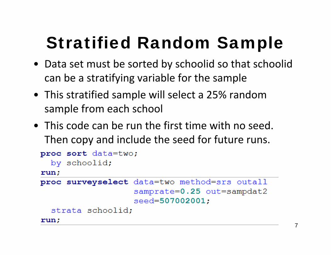
Stratified Random Sample• Data set must be sorted by schoolid so that schoolid can be a stratifying variable for the sample

• This stratified sample will select a 25% random sample from each school

• This code can be run the first time with no seed. Then copy and include the seed for future runs.

7

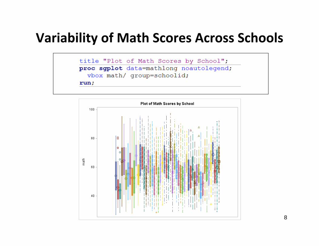
Variability of Math Scores Across Schools

8

Variability of Math Scores by Schools

• There appears to be a fair amount of variability between schools in terms of their math scores

• We will want to include a random intercept for each school to capture this variability and to allow the scores for students within the same school to be correlated

• We do not have school-level variables to include in this model, but we may want to explore further whether any school-level variables (e.g., Rural/Urban) can explain these differences between schools 9

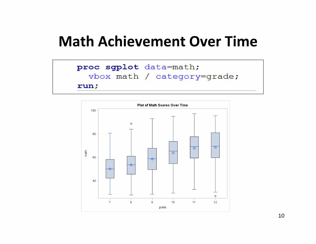
Math Achievement Over Time

10

Math Achievement Over Time

• Math achievement increases over time• This is expected• We want to explore whether the rate of increase

over time differs by child and whether child covariates or parent covariates can help to explain differences in the rate of increase

11

Spaghetti Plots

12

Spaghetti Plots for Each Child

• There is a general increase in math achievement over time across students

• Some students have a steeper slope over time and others have a lower slope

• The spaghetti plots emphasize the erratic nature of the math scores (they are not all smoothly increasing for each child)

• A random sample of children would more clearly show individual patterns (we don’t show this)

13

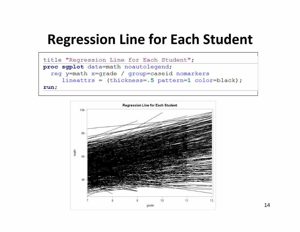
Regression Line for Each Student

14

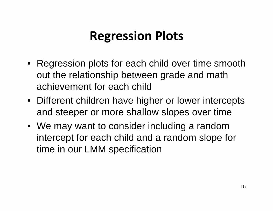
Regression Plots

• Regression plots for each child over time smooth out the relationship between grade and math achievement for each child

• Different children have higher or lower intercepts and steeper or more shallow slopes over time

• We may want to consider including a random intercept for each child and a random slope for time in our LMM specification

15

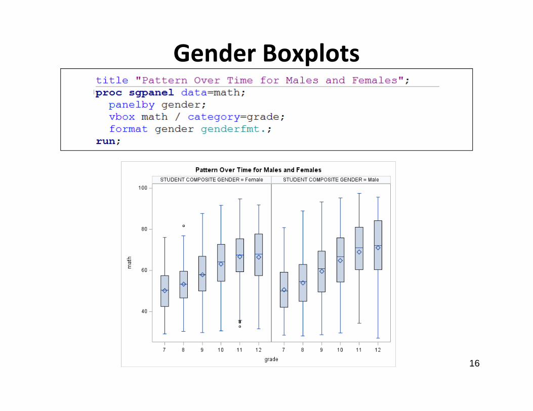
Gender Boxplots

16

Box Plots for Gender Over Time

• The paneled boxplot shows that math scores increase generally for boys and for girls

• The variability at each grade does not appear to differ, nor does it appear to be different for boys vs. girls

• We next look at a regression line over time for males and for females

17

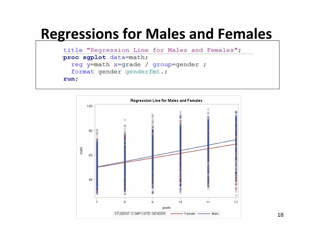
Regressions for Males and Females

18

Regression Lines for Gender• Based on these regression plots, it appears that

gender does not explain much of the variability in math achievement scores

• Boys and girls appear to start out at a very similar level of math achievement

• The slope over time appears to be a bit steeper for boys than for girls, so we may expect to see a difference between boys and girls by 12th

grade (or sooner)• We may want to include an interaction between

gender and grade to see if this is true19

Regressions for Parent Education

20

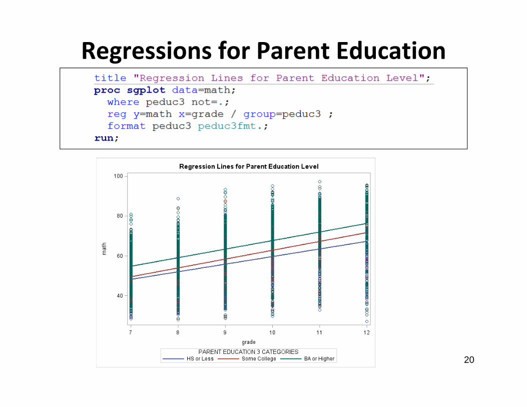
Regression Lines for Parent Education• Based on these regression plots, it appears that

children of parents with a BA or greater education level tend to do better in math achievement at 7th grade than children in the other two categories.

• As time goes on, the difference between BA or greater and some college appears to diminish while the difference between HS or less and some college appears to get wider

• We may want to include an interaction between time and parent education to see if this is true

21

Regressions for Likes Math Levels

22

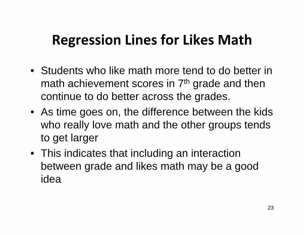
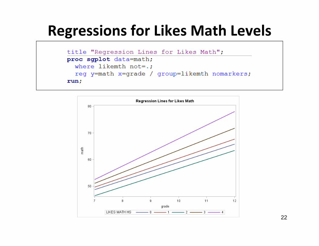
Regression Lines for Likes Math

• Students who like math more tend to do better in math achievement scores in 7th grade and then continue to do better across the grades.

• As time goes on, the difference between the kids who really love math and the other groups tends to get larger

• This indicates that including an interaction between grade and likes math may be a good idea

23

Regression Line for Parent Academic Push

24

Is Parent Academic Push Negatively Related to Math

Achievement?• We expect that children of parents who push

their children more academically will do better in math, but we see an apparent negative relationship between parent academic push and math achievement

• Is this real?• Recall that parent academic push was

measured at each time point• We need to see the effects of parent academic

push within each grade25

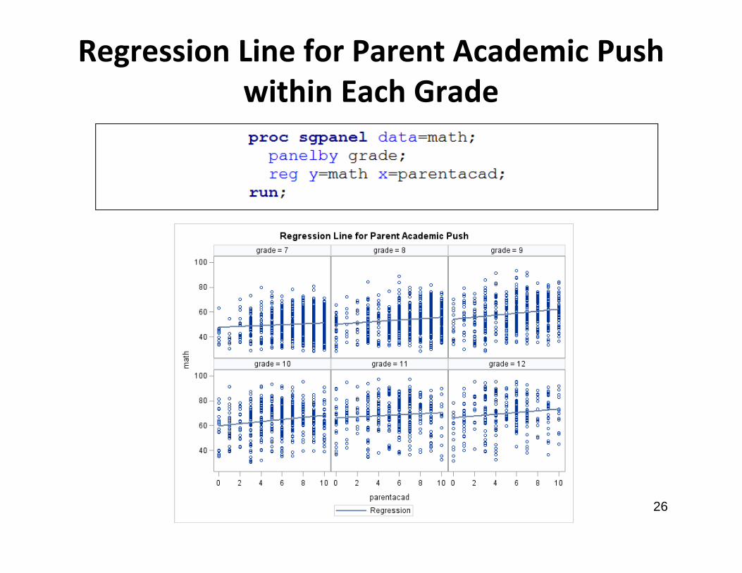
Regression Line for Parent Academic Push within Each Grade

26

Is Parent Academic Push Actually Negatively Related to

Math Achievement?• Within each grade, the relationship between

parent academic push and math achievement is positive, yet the overall relationship is negative

• How can this be?• Let’s look at descriptive statistics for parent

academic push and for math achievement for each grade

27

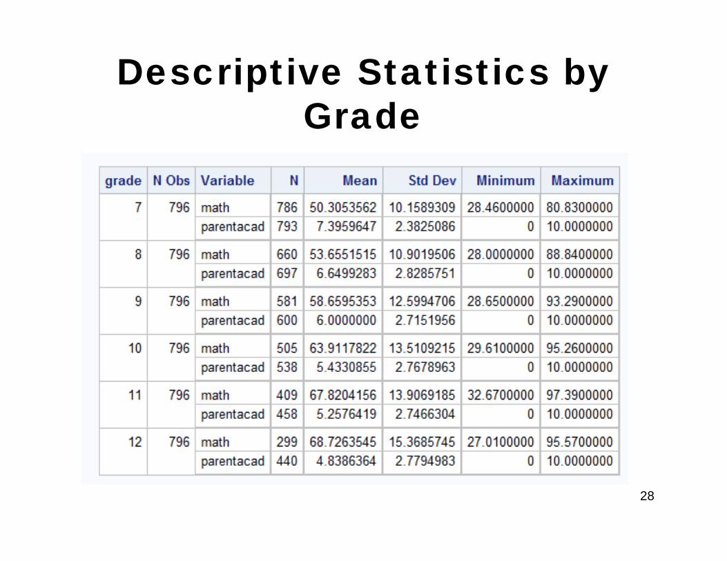
Descriptive Statistics by Grade

28

What is Going On?

• Notice that math achievement is increasing across grades (as we saw in the previous graphs)

• Parent academic push is decreasing over time (parents are apparently pushing their kids less academically as they grow older)

• The result is that overall it looks like kids of parents who push more do worse, but actually, within the same grade, kids of parents who push more have higher math scores for every grade

29

What is Going On?

• Notice that math achievement is increasing across grades (as we saw in the previous graphs)

• Parent academic push is decreasing over time (parents are apparently pushing their kids less academically as they grow older)

• The result is that overall it looks like kids of parents who push more do worse, but actually, within the same grade, kids of parents who push more have higher math scores for every grade

30

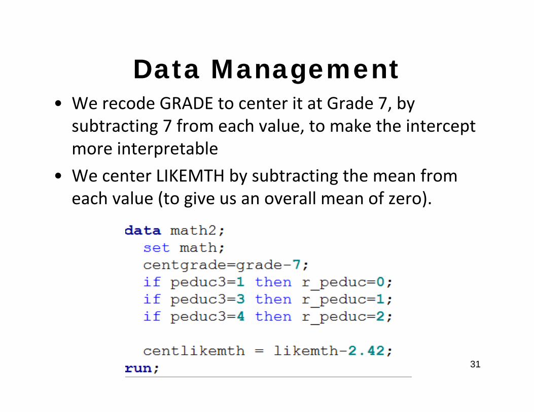
Data Management• We recode GRADE to center it at Grade 7, by subtracting 7 from each value, to make the intercept more interpretable 

• We center LIKEMTH by subtracting the mean from each value (to give us an overall mean of zero).

31

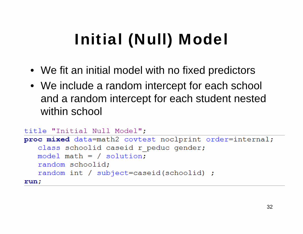
Initial (Null) Model

• We fit an initial model with no fixed predictors• We include a random intercept for each school

and a random intercept for each student nested within school

32

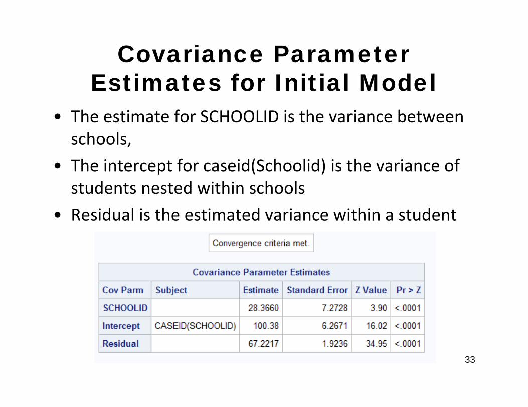
Covariance Parameter Estimates for Initial Model

• The estimate for SCHOOLID is the variance between schools,

• The intercept for caseid(Schoolid) is the variance of students nested within schools

• Residual is the estimated variance within a student

33

Fixed Effects Estimates for Initial Model

• The Intercept represents the predicted mean of math achievement across all grades, for an average school and an average student

34

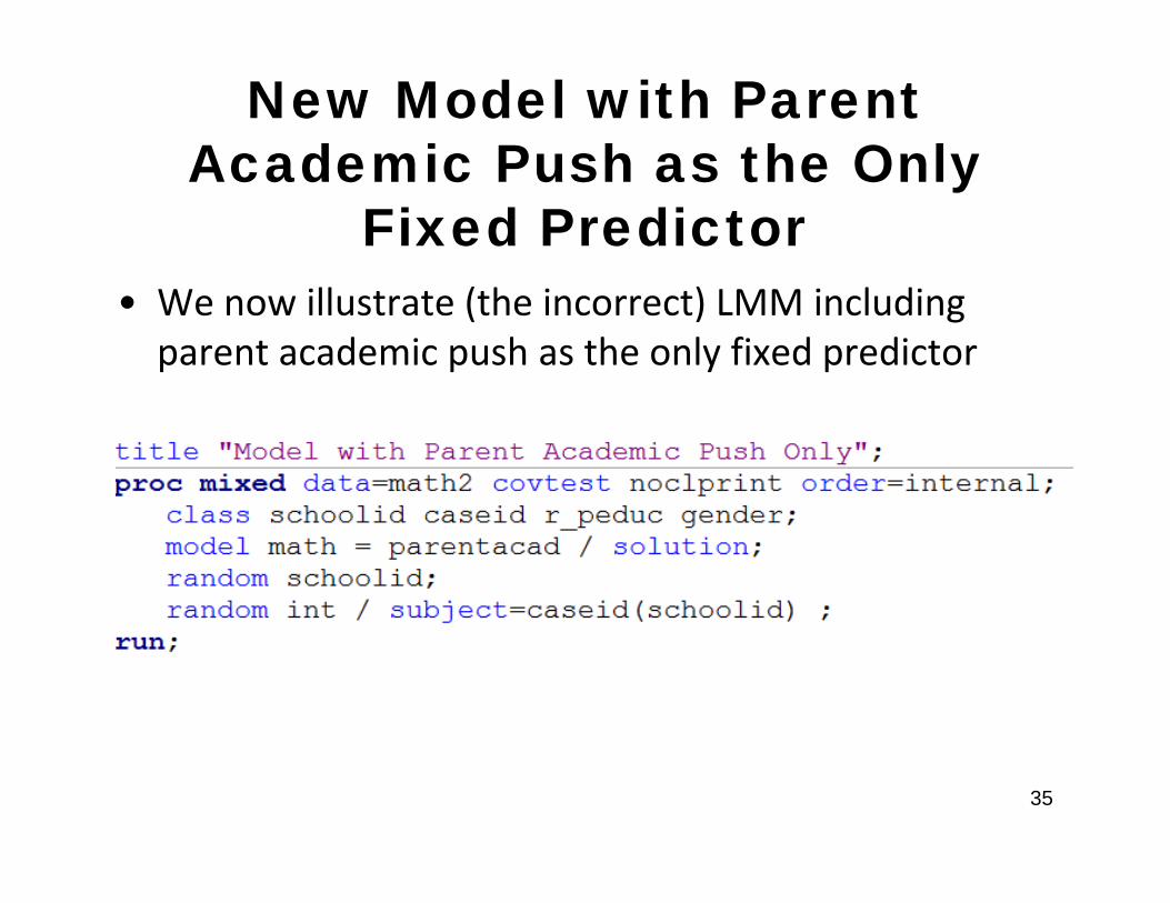
New Model with Parent Academic Push as the Only

Fixed Predictor• We now illustrate (the incorrect) LMM including parent academic push as the only fixed predictor

35

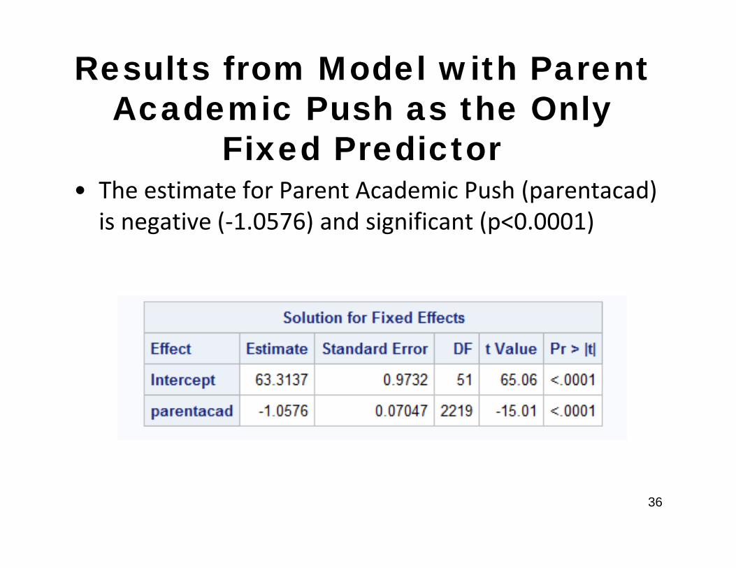
Results from Model with Parent Academic Push as the Only

Fixed Predictor• The estimate for Parent Academic Push (parentacad) is negative (‐1.0576) and significant (p<0.0001)

36

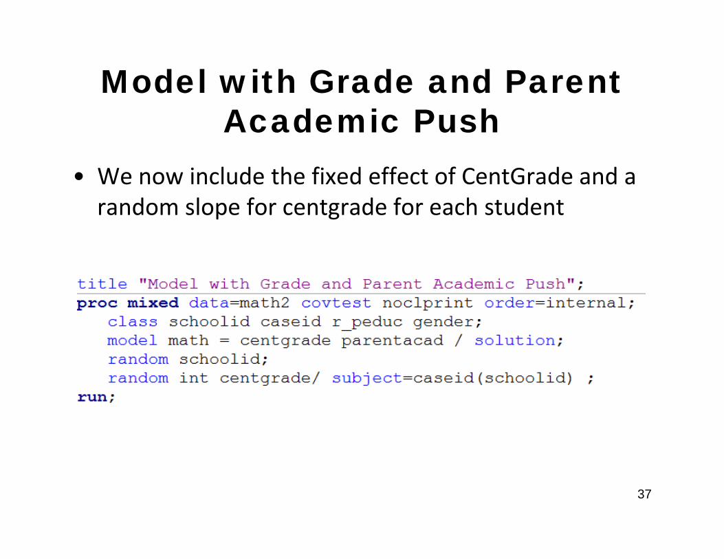
Model with Grade and Parent Academic Push

• We now include the fixed effect of CentGrade and a random slope for centgrade for each student

37

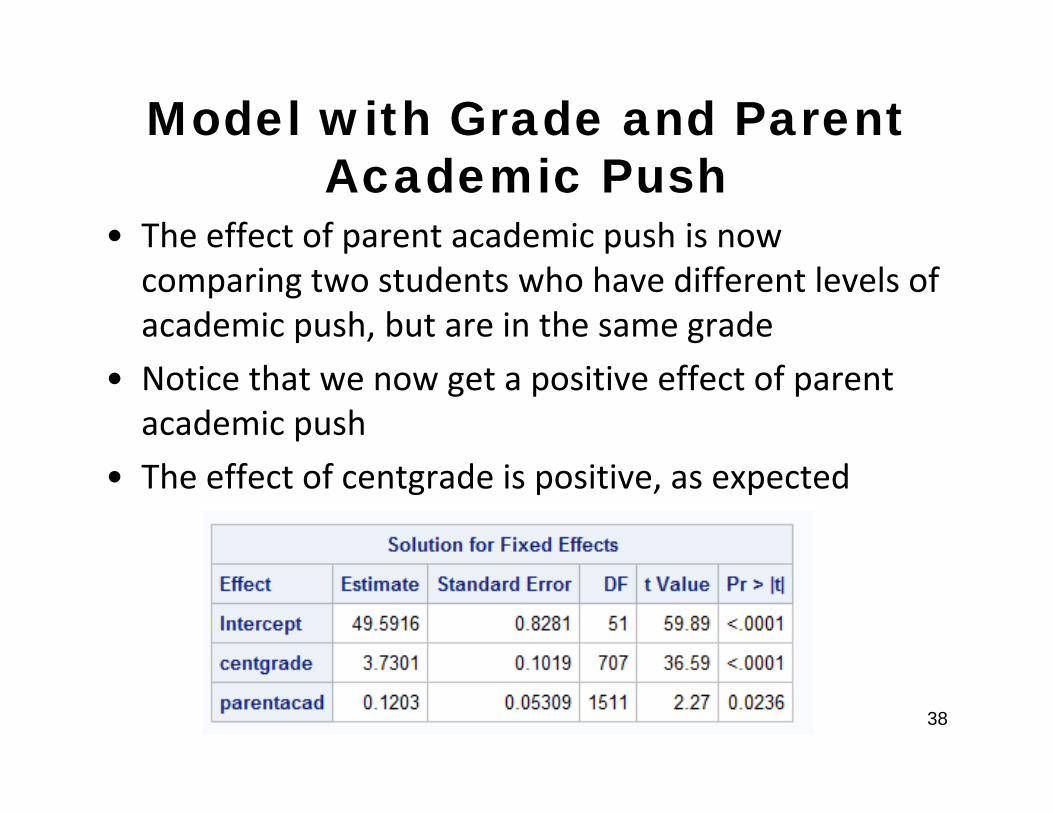
Model with Grade and Parent Academic Push

• The effect of parent academic push is now comparing two students who have different levels of academic push, but are in the same grade

• Notice that we now get a positive effect of parent academic push

• The effect of centgrade is positive, as expected

38

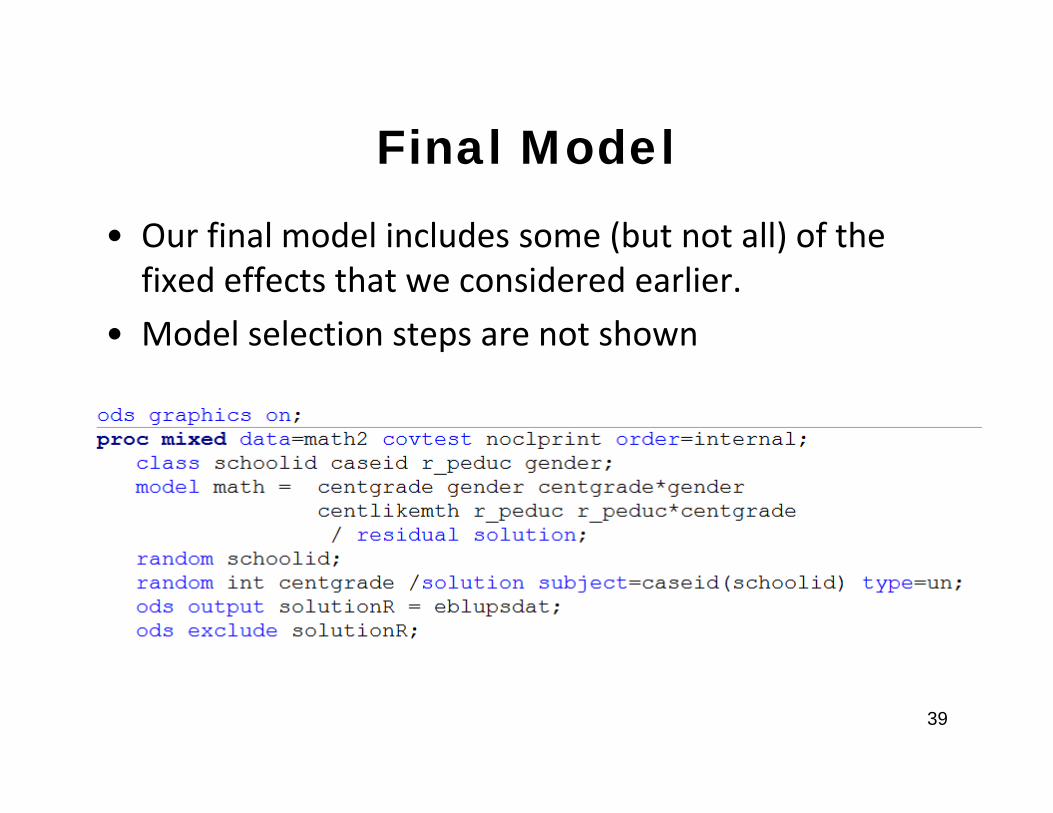
Final Model

• Our final model includes some (but not all) of the fixed effects that we considered earlier.

• Model selection steps are not shown

39

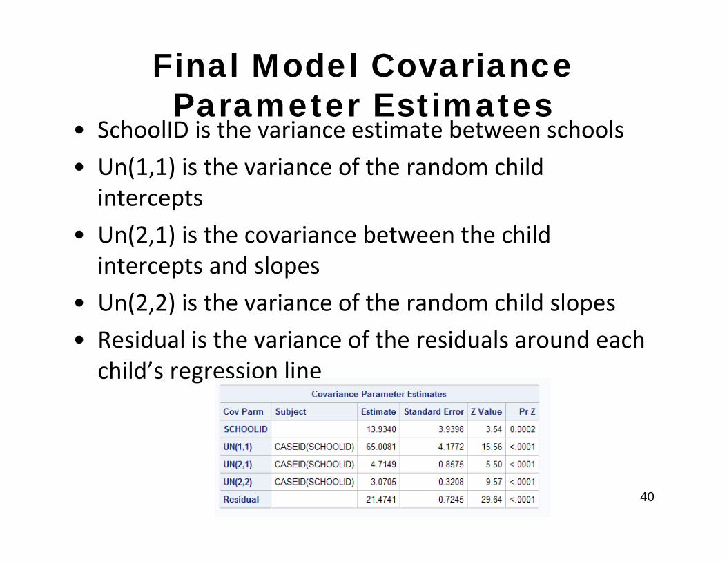
Final Model Covariance Parameter Estimates

• SchoolID is the variance estimate between schools• Un(1,1) is the variance of the random child intercepts

• Un(2,1) is the covariance between the child intercepts and slopes

• Un(2,2) is the variance of the random child slopes• Residual is the variance of the residuals around each child’s regression line

40

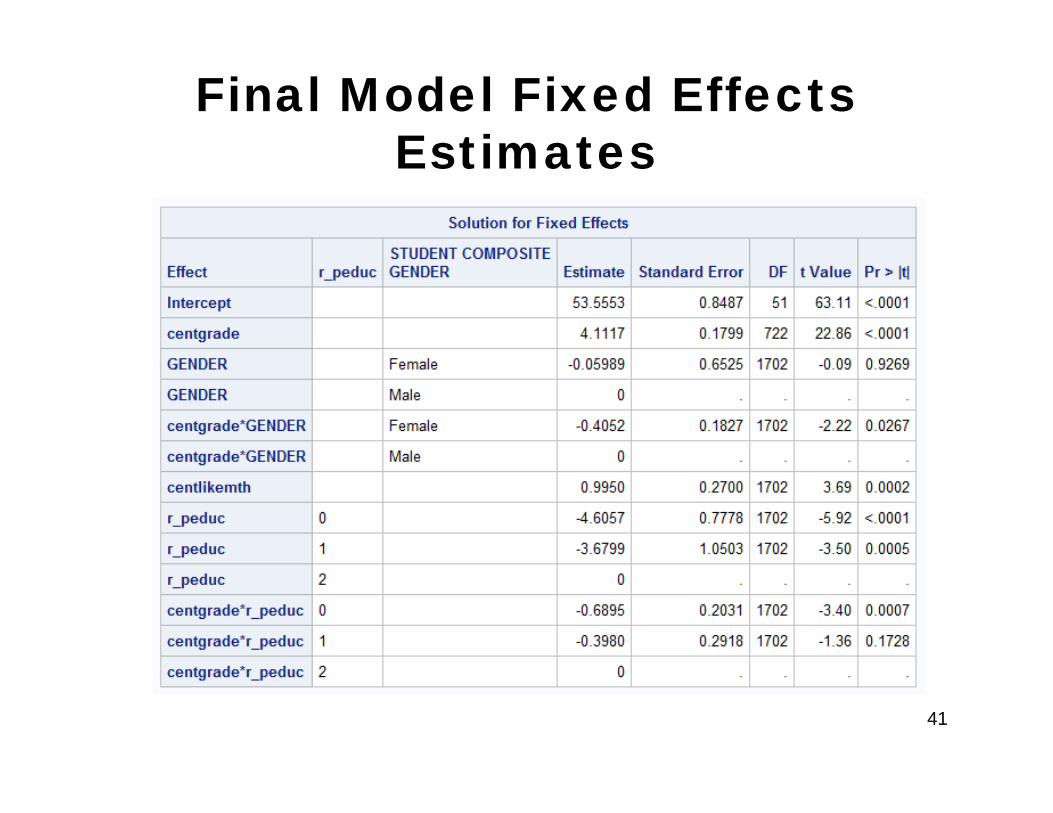
Final Model Fixed Effects Estimates

41

Final Model Residual Diagnostics

42

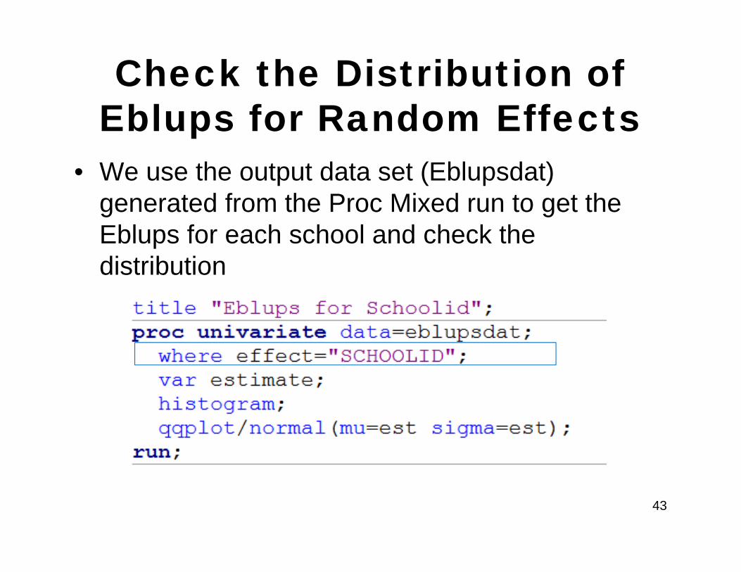
Check the Distribution of Eblups for Random Effects

• We use the output data set (Eblupsdat) generated from the Proc Mixed run to get the Eblups for each school and check the distribution

43

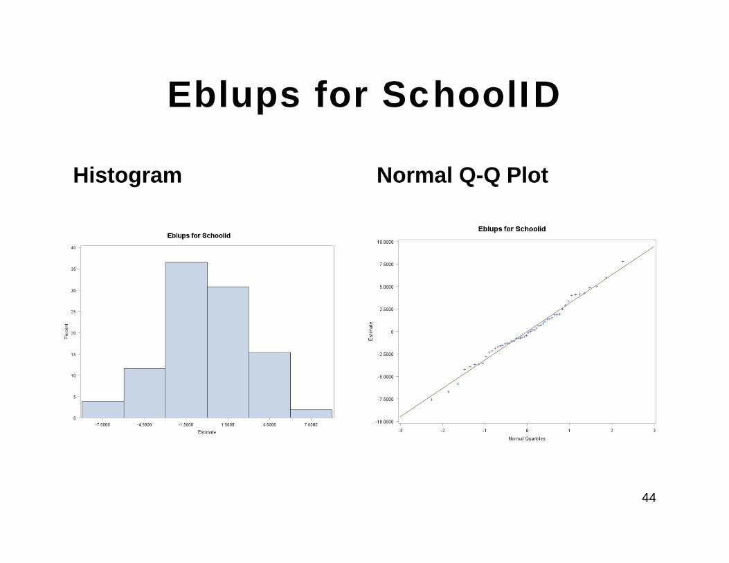
Eblups for SchoolID

Histogram Normal Q-Q Plot

44

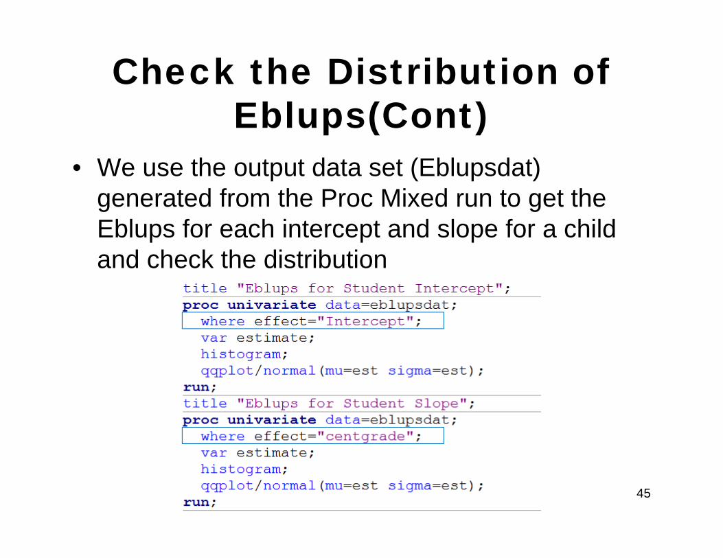
Check the Distribution of Eblups(Cont)

• We use the output data set (Eblupsdat) generated from the Proc Mixed run to get the Eblups for each intercept and slope for a child and check the distribution

45

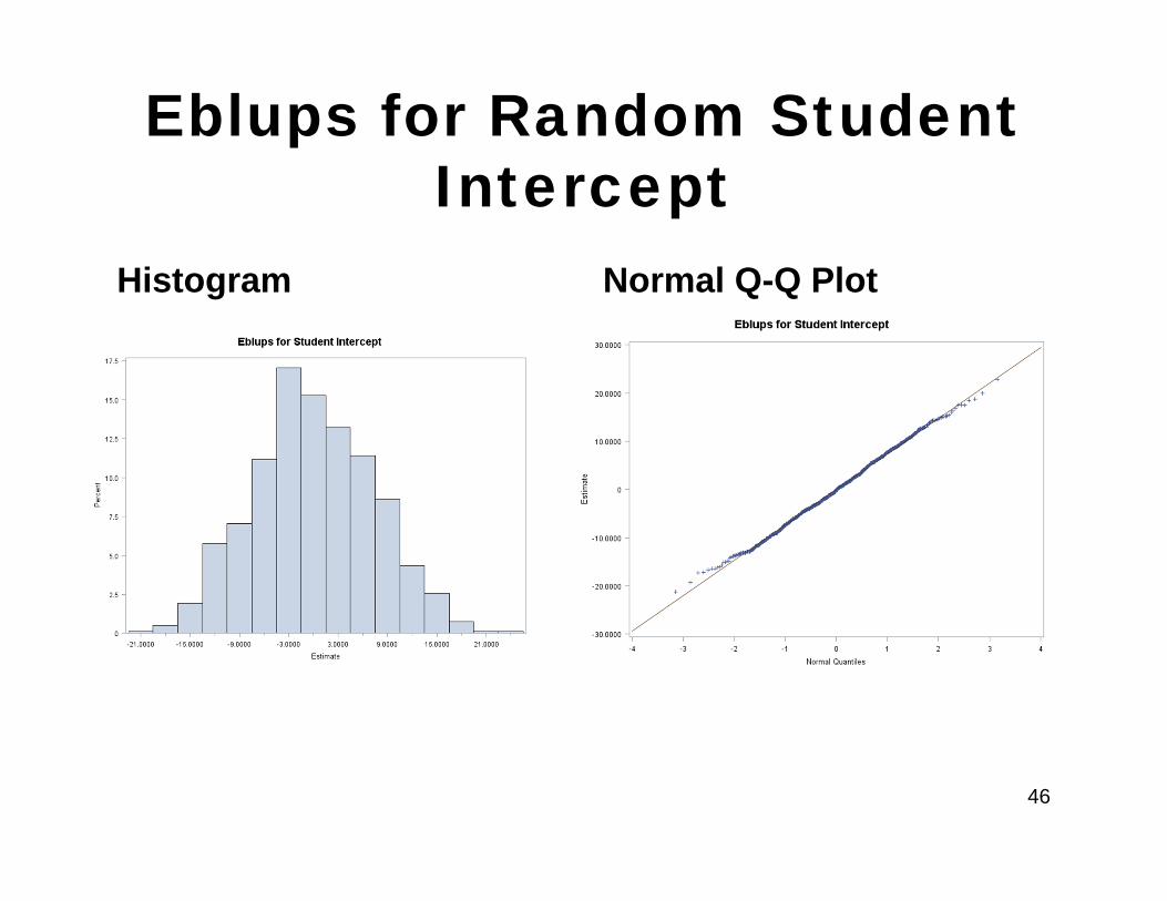
Eblups for Random Student Intercept

Histogram Normal Q-Q Plot

46

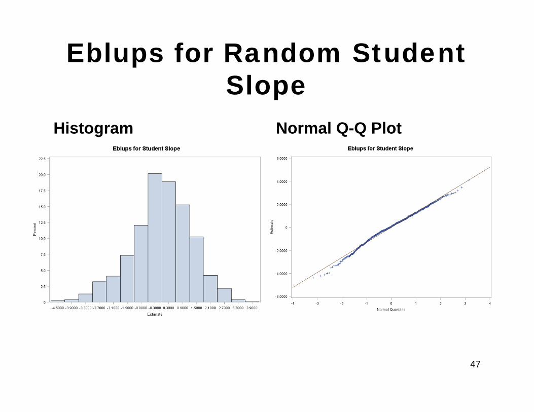
Eblups for Random Student Slope

Histogram Normal Q-Q Plot

47

Summary• Proc Mixed is a flexible tool for fitting models for clustered‐longitudinal data

• Care must be taken when including time‐varying predictors in the model to be sure that the interpretation of their effects is correct

• Graphics can help to understand the data before the model‐fitting process begins 

48

References: Software and Data

• The output, code and data analysis for this presentation were generated using SAS/STAT software, Version 9.3 (TS1M0) of the SAS System for Windows. Copyright ©2002-2010 SAS Institute Inc. SAS and all other SAS Institute Inc. product or service names are registered trademarks or trademarks of SAS Institute Inc., Cary, NC, USA.

• The data used for these examples were derived from the Longitudinal Study of American Youth (ICPSR 30263)

• Kathy Welch is responsible for any errors or omissions in this analysis

49

References• Verbeke, G., and Molenberghs, G. Linear Mixed

Models for Longitudinal Data, Springer, New York, 2000.

• West, Brady T., Welch, Kathleen B., Galecki, Andrzej T., Linear Mixed Models: A Practical Guide, Chapman & Hall, 2007.

50