Using R to Keep it Simple: Exploring Structure in Multilevel Datasets

Jake BowersDept of Political Science and Center for Political Studies

University of Michigan

Version of September 11, 2004

Point 1: Before starting R have a question you want to answer.

In the United States, the relationship between education and political participation in thecross-section is well known: better educated people tend to be the types that get involvedin politics. Extant theories suggest that this relationship exists because (1) people who arebetter educated have more of the skills they need to do the work of political participation(Verba, Schlozman and Brady, 1995) and (2) people who are better educated are more likelyto know other political actors, i.e. they have higher status in the kinds of social networksthat matter for political involvement (Nie, Junn and Stehlik-Barry, 1996; Rosenstone andHansen, 1993; Huckfeldt, 1979).

If we looked at the relationship between education and participation in other countries,would these theories travel? Would education as “civic skills,” such as knowing how to writeletters or chair meetings, have the same impact on civic activity in a country where nearlyeveryone is highly educated as in a country where very few people are literate? Probablynot. Would education matter as much in a place where social status is conferred at birthas it does in a place where social status is tied to a college degree? Probably not. Thesesuppositions raise the question about what might be determining who participates across avariety of places, where education plays different roles in society. Answers to this questionmight tell us something new about the societal bases of political activity, as well as providingnew perspectives on 50 years worth of literature based largely on studies of ordinary citizensin the USA.

The question I posed about whether the theories of political participation travel is in essencea question about whether a relationship between variables measured at one level (amongordinary people) depends in some way on variables measured at another level (among coun-tries). This article is written now because we are finally getting data to address suchquestions directly on a large scale via the Comparative Study of Electoral Systems (CSESSecretariat), the World Values Survey (Inglehart et al.), the African/Euro/Latino Barome-ters (The Afrobarometer Network; European Commission; Lagos and The LatinobarometroCorporation), and others. Also, within the study of domestic politics, more and more re-searchers are gathering data on attributes of both citizens and the electoral districts or othergeographies in which they are embedded. In fact, I wager a bottle of Kwak (a Belgian beer)that the number of articles in political science journals concerned with quantitative analysisof datasets with more than one type of unit of analysis has more than doubled in the last10 years.

A dataset used to answer questions about people nested within geographies tends to havefewer countries/districts/states (i.e., macro-level units) than individuals/towns/firms (i.e.,micro-level units). And analyses based on such datasets tend to focus on how differencesacross macro-units somehow condition or influence the differences within macro-units.1 Toaddress the question I posed earlier, I use the World Values Surveys and European ValuesSurveys 1999-2001 combined file (ICPSR # 3975) for the micro-level variables of educa-tional attainment and political participation. For macro-level data I use information from

1I am leaving time out of this article to keep it simple.

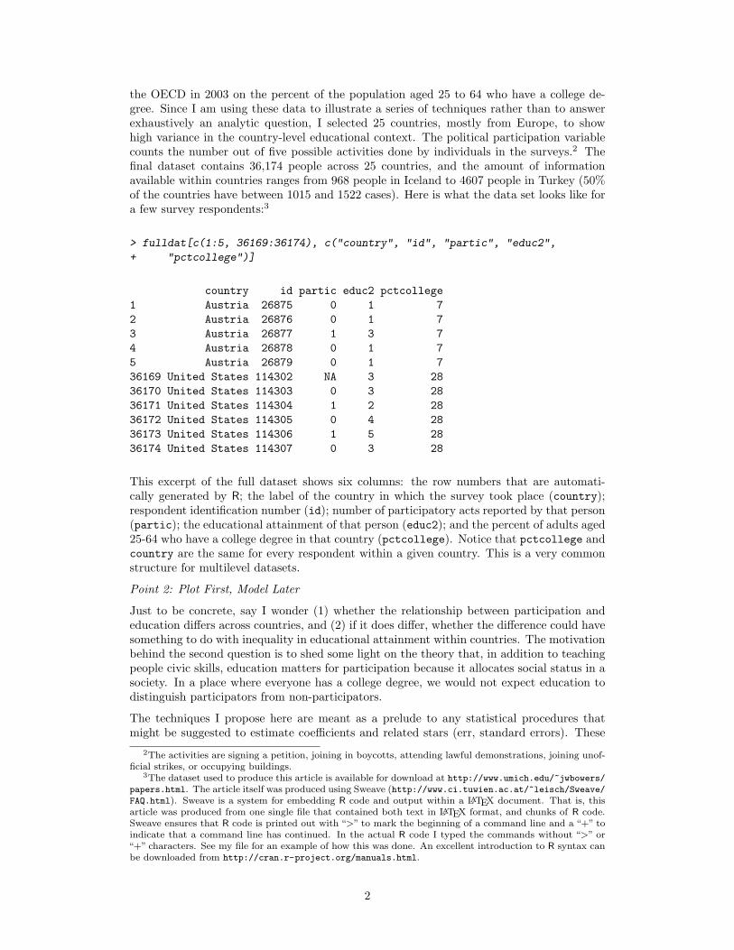
the OECD in 2003 on the percent of the population aged 25 to 64 who have a college de-gree. Since I am using these data to illustrate a series of techniques rather than to answerexhaustively an analytic question, I selected 25 countries, mostly from Europe, to showhigh variance in the country-level educational context. The political participation variablecounts the number out of five possible activities done by individuals in the surveys.2 Thefinal dataset contains 36,174 people across 25 countries, and the amount of informationavailable within countries ranges from 968 people in Iceland to 4607 people in Turkey (50%of the countries have between 1015 and 1522 cases). Here is what the data set looks like fora few survey respondents:3

> fulldat[c(1:5, 36169:36174), c("country", "id", "partic", "educ2",

+ "pctcollege")]

country id partic educ2 pctcollege1 Austria 26875 0 1 72 Austria 26876 0 1 73 Austria 26877 1 3 74 Austria 26878 0 1 75 Austria 26879 0 1 736169 United States 114302 NA 3 2836170 United States 114303 0 3 2836171 United States 114304 1 2 2836172 United States 114305 0 4 2836173 United States 114306 1 5 2836174 United States 114307 0 3 28

This excerpt of the full dataset shows six columns: the row numbers that are automati-cally generated by R; the label of the country in which the survey took place (country);respondent identification number (id); number of participatory acts reported by that person(partic); the educational attainment of that person (educ2); and the percent of adults aged25-64 who have a college degree in that country (pctcollege). Notice that pctcollege andcountry are the same for every respondent within a given country. This is a very commonstructure for multilevel datasets.

Point 2: Plot First, Model Later

Just to be concrete, say I wonder (1) whether the relationship between participation andeducation differs across countries, and (2) if it does differ, whether the difference could havesomething to do with inequality in educational attainment within countries. The motivationbehind the second question is to shed some light on the theory that, in addition to teachingpeople civic skills, education matters for participation because it allocates social status in asociety. In a place where everyone has a college degree, we would not expect education todistinguish participators from non-participators.

The techniques I propose here are meant as a prelude to any statistical procedures thatmight be suggested to estimate coefficients and related stars (err, standard errors). These

2The activities are signing a petition, joining in boycotts, attending lawful demonstrations, joining unof-ficial strikes, or occupying buildings.

3The dataset used to produce this article is available for download at http://www.umich.edu/~jwbowers/papers.html. The article itself was produced using Sweave (http://www.ci.tuwien.ac.at/~leisch/Sweave/FAQ.html). Sweave is a system for embedding R code and output within a LATEX document. That is, thisarticle was produced from one single file that contained both text in LATEX format, and chunks of R code.Sweave ensures that R code is printed out with “>” to mark the beginning of a command line and a “+” toindicate that a command line has continued. In the actual R code I typed the commands without “>” or“+” characters. See my file for an example of how this was done. An excellent introduction to R syntax canbe downloaded from http://cran.r-project.org/manuals.html.

2

techniques will help you decide which kind of analysis you will eventually want to conductand which modeling assumptions are more or less tenable. The idea is simple: run a re-gression for each country and then plot the coefficients.4 The idea of running 25 differentregressions, one per country, and making at least 25 different plots is enough to make mostpeoples’ eyes glaze over. This is where R (R Development Core Team, 2004) makes life mucheasier. The following 2 lines of R code run 25 regressions, collect the 25 regression objectsin a list named theregs, and add names to the list object for the appropriate countries(naming things turns out to make life a bit easier down the road).5

> theregs <- lapply(unique(fulldat$country), function(x) {

+ lm(partic ~ educ2, data = fulldat[fulldat$country == x, ])

+ })

> names(theregs) <- unique(fulldat$country)

To make things easier for plotting, I collect the coefficients from the regressions into amatrix called coefmat and the standard errors into a matrix called semat. Then, I combinecoefficients, standard errors, and country-level information into a data frame that I canuse for plotting. I also make a new macro-level variable called educgroupsQ which breaksthe country-level educational context variable into three groups — low, middle, and high.Finally, I print the first three rows of the coefmat matrix.

> coefmat <- matrix(unlist(lapply(theregs, coef)), ncol = 2, byrow = TRUE,

+ dimnames = list(names(theregs), c("Intercept", "Educ")))

> semat <- matrix(unlist(lapply(theregs, function(x) summary(x)$coef[,

+ "Std. Error"])), ncol = 2, byrow = TRUE, dimnames = list(names(theregs),

+ c("SEIntercept", "SEEduc")))

> coefsedf <- data.frame(coefmat, semat)

> coefsedf$country <- factor(row.names(coefsedf))

> coefdf <- merge(coefsedf, themacrodat, by = "country")

> row.names(coefdf) <- as.character(coefdf$country)

> coefdf$educgroupsQ <- cut(coefdf$pctcollege, quantile(coefdf$pctcollege,

+ p = c(0, 0.25, 0.75, 1)), include.lowest = TRUE)

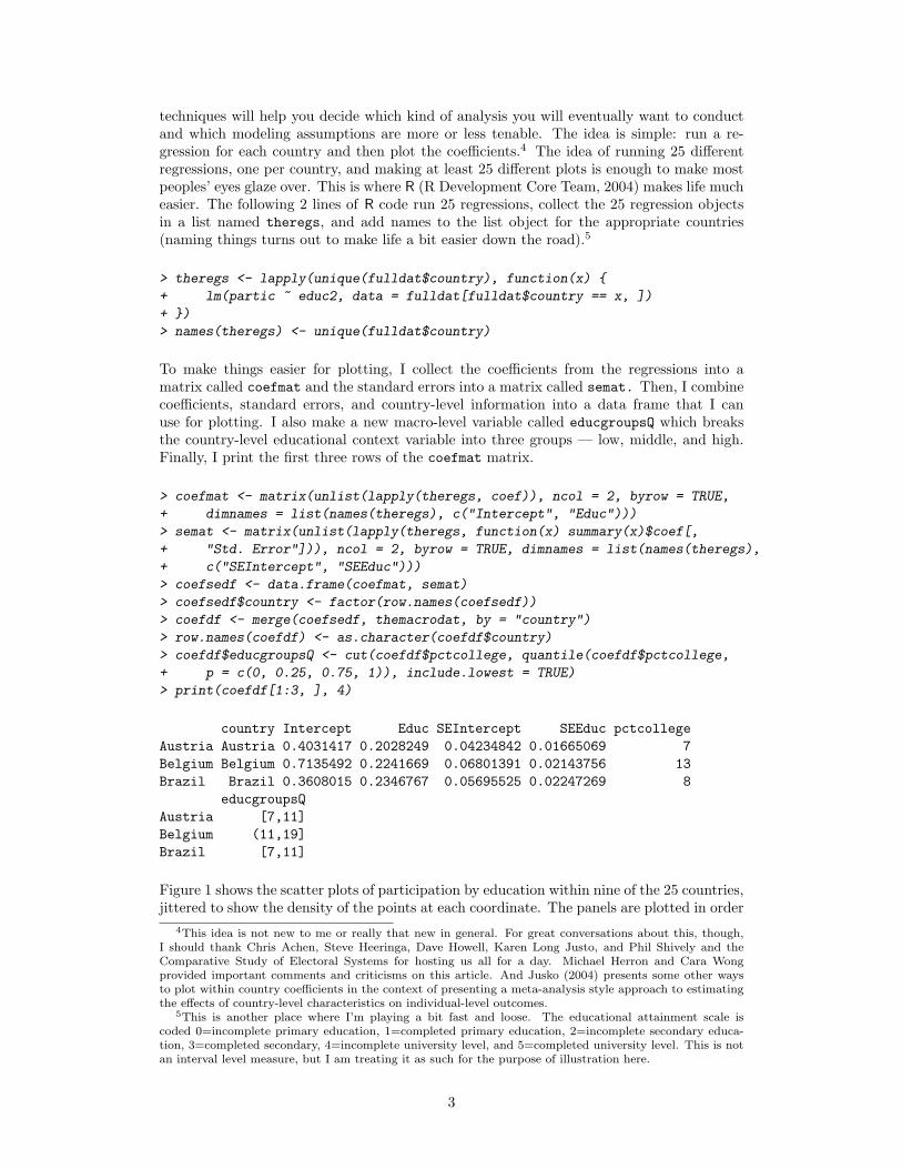
> print(coefdf[1:3, ], 4)

country Intercept Educ SEIntercept SEEduc pctcollegeAustria Austria 0.4031417 0.2028249 0.04234842 0.01665069 7Belgium Belgium 0.7135492 0.2241669 0.06801391 0.02143756 13Brazil Brazil 0.3608015 0.2346767 0.05695525 0.02247269 8

educgroupsQAustria [7,11]Belgium (11,19]Brazil [7,11]

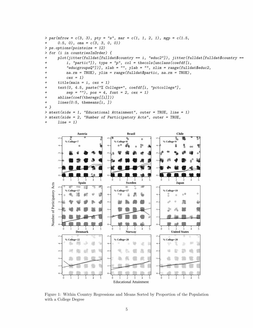
Figure 1 shows the scatter plots of participation by education within nine of the 25 countries,jittered to show the density of the points at each coordinate. The panels are plotted in order

4This idea is not new to me or really that new in general. For great conversations about this, though,I should thank Chris Achen, Steve Heeringa, Dave Howell, Karen Long Justo, and Phil Shively and theComparative Study of Electoral Systems for hosting us all for a day. Michael Herron and Cara Wongprovided important comments and criticisms on this article. And Jusko (2004) presents some other waysto plot within country coefficients in the context of presenting a meta-analysis style approach to estimatingthe effects of country-level characteristics on individual-level outcomes.

5This is another place where I’m playing a bit fast and loose. The educational attainment scale iscoded 0=incomplete primary education, 1=completed primary education, 2=incomplete secondary educa-tion, 3=completed secondary, 4=incomplete university level, and 5=completed university level. This is notan interval level measure, but I am treating it as such for the purpose of illustration here.

3

of the percent of their population aged 25-64 who have a college degree (with the UnitedStates having the highest proportion and Austria the lowest). The plots for the countries inthe lowest education group are colored black, the middle group is colored dark gray, and thehighest group is colored light gray. Each panel contains a regression line (the straight one)and a line connecting the mean participation levels at each level of educational attainment(the not straight one). I included the line of means as a check for non-linear relationships.The percent attending college in the country is also printed in each panel.

> themeans <- tapply(fulldat$partic, list(country = fulldat$country,

+ educ2 = fulldat$educ2), function(x) mean(x, na.rm = TRUE))

> somecountries <- c("Austria", "Brazil", "Chile", "Spain", "Sweden",

+ "Japan", "Denmark", "Norway", "United States")

> smallcoefdf <- coefdf[coefdf$country %in% somecountries, ]

> countriesInOrder <- as.character(smallcoefdf$country[order(smallcoefdf$pctcollege)])

> thecols <- gray(c(0.1, 0.5, 0.8))

> quartz()

4

> par(mfrow = c(3, 3), pty = "s", mar = c(1, 1, 2, 1), mgp = c(1.5,

+ 0.5, 0), oma = c(3, 3, 0, 0))

> ps.options(pointsize = 12)

> for (i in countriesInOrder) {

+ plot(jitter(fulldat[fulldat$country == i, "educ2"]), jitter(fulldat[fulldat$country ==

+ i, "partic"]), type = "p", col = thecols[unclass(coefdf[i,

+ "educgroupsQ"])], xlab = "", ylab = "", xlim = range(fulldat$educ2,

+ na.rm = TRUE), ylim = range(fulldat$partic, na.rm = TRUE),

+ cex = 1)

+ title(main = i, cex = 1)

+ text(0, 4.5, paste("% College=", coefdf[i, "pctcollege"],

+ sep = ""), pos = 4, font = 2, cex = 1)

+ abline(coef(theregs[[i]]))

+ lines(0:5, themeans[i, ])

+ }

> mtext(side = 1, "Educational Attainment", outer = TRUE, line = 1)

> mtext(side = 2, "Number of Participatory Acts", outer = TRUE,

+ line = 1)

●

●

●

●●

●●

● ● ●

● ●●

●

●●

●● ●

●

●●

●

●

●

●

●

●

●

●

● ●

● ●

●

●

● ●●

●

●

●

●●●

●●

●

●

●

●

●●

●●

●●

●

●

●

●

●

●

●

●

●

●●

●

●

●

● ●

●

●

● ●

●

●● ●●

●

●

●

●

●●

●● ●●

●

●

●●●

●

●

●●● ●●

● ● ●●●

●

●

●

●

●

●

●●

●

●

●

●●

●

●

●

●

●●

●

●

●

●

●

●

●●

●

●

●

●●

●

●

●

●●●●

●

● ●

●●

●

●●

●●

●

●

●

●

●

●●●

●●

●●●

●

●

●

●

●● ●

●

●

●

●●

●

●

●

●●

●

● ●

●

●

●

●

●●●

●●

●

●● ●

●●

●

●

●●

●●

●

●

●●●

●●

●

●

●●●

●

●

●●

●

●

●●

●●

●

●

●

●

●

●

●

●

●

●

●

●●

●

●

●●

●●

●

●

●●

●

●

●

●●

●

●

●

●

●●

●

●●

●●

●●

●

●

●

●●

●

●

● ●●

●

●● ●

●● ●

●

●

●

●●

●●●

● ●

●

●

●●

●●●

●

●

●

●

●

●

●

●

●●

●

●

●

●

● ●

●

●

●

●

●

●●

●

●

●●

●●

●

●

●

●●

●

●●●

●●

●

●

● ●

●

●●

●

●

● ●● ●

●●●

●

●

●

●

●

●

●

●

●

●

●●

●

●

●

●

●

●

●

●●

●

●

●

●

●●

●

●

●

●●

●●

●● ●●

●

●

●●●

●●

●

●●●●●●

●

●

●

●

●●

●

●

●

●

●

●

●●

●

●

●● ●●

●●●

●

●

●

●

●

●

●

●●●●

●●●

●

● ●

●

●

●

●

●

●

●●

●●●

●●

●

●●

●

●

●

●

●●

●

●●

●●

●

●

●

●

●●

●

●

●

●

●

●

●

●

●●

●●

● ●●

●●

●●

●●

●

●

●●

●

●●

●

●

●

● ●

●

●●

●

●●

●●●

●

●

●

●●

●

●

●

●

●

●

●●

●

●

●

●●

●●

●● ●●

●

●

●●

●

●

●

●

●●

●●

●●

●

●

● ●

●●

●

●●

●●●

●

●

●

●● ● ●

●

●●●●

●

●●

●

●

● ●

●

●

●

●

●

●

●

●●

●

●

● ●●

●

●●

●

●

●

●

●

●

●●

●●

●

●● ●●●●

●

●●● ●

●

●

●

●

●

●●

●

●

●

●

●

●

●

●

● ●●

●

●

●

●●● ●

●

●●

●●

●●●

●

●●● ●

●

●

●

●●●●●

●

●●

●

●●

●●

●

● ●

●

●●

● ●●

●

●

●●

●

● ●

●●

●

●●

●

●●●

●●

●●●

●

●●

● ●●

●

●●

●

●

●

●

●

●

●●

●

●

●

●● ●

●●

●

●

●

●

●

●

●

●

●

●

●

● ●

●●

● ●

●

●

●

●

●

●

●

●

●●

●●

●

●

●

●

●●●

●

●

●

● ●●

●●●

●●● ●● ●

●●

●●

● ●●

●●

●

●●

●

●

●

● ●●●

●

●●

●

●

● ● ●

●

●

●

●●

●

●●

●●

●

●

●●

●●●

●●

●

●

●

●

●

●● ●

●●

●●●

●

●

●

●●

●

●

●●

●

●

●

●

●●●

● ●

●

● ●●

●

●

●

●

●

●● ●

●

●●

●

●●●

●

●

●

●

●

●●●

●

●● ●

●

●

●●

●

●

●●●●

●

●

●

●●

●

●

●

●

●

●

●●

●●

●

●

●●

●

●●●

●

● ●

●

●

●●●

●

● ●

●

●●

●

●

●●

●

●

●●

●

●

●

●

●

●

●

●

●

●

●

●

●

●

●

● ●

●

●

●●

●●●

●

●● ●

●

●

● ●●●

●

●●

●

●

●

●

●

●

●

●●●

●

●

●

●

●

● ●

●

●

●

●

●

● ●

●

●● ●

●

●

●

●

●●

●

●

●

●

●

●

●

●

●

●

●

●●

●

●

●

●●

●●

●

●

●●

●

●

●

●

●

●

●

●

●●

●●

●

●●

●

●

●

●

●●●

●

●● ●

●

●●●

●●●

●

●●●

●

●

●

●●

●

● ●●

●

●

●●●

●

●

●

●

●

●

●

●

●●

●●● ●

●

●●

●

● ●

●●● ●

●

●

●

●

●

●

●

●

●

●

●

●

●

●● ●

●

●

●

●●

●

●

●

●

●

●

●

●

●

●

● ●●●

●

●

●

●

●

●

●●

●

●

●

●

●

●●

●●● ●

●● ●

●

●

●

●●

●

●

●●●

●

●

● ●●

●

●●

●

●●●

●

●●

●

●●●

●

●

●

●

●

●● ●

● ●

●

●●●

●● ●

●

● ●●

●

●

●

●

●

●

●

●

●

●

● ●●

●●

●

●

●

●

●●

●

●●●

●

●

●

●●

●

●

●

●

●

●●●

●

●

●

●

●

●

●

●

●●

● ●

●●

●

●

●

●●

●

●●

●

●

●

●

●

●

●●●

●●

●●

●

●●●●

●

●

●

● ●

●●

●

●

●

●●●

●

●

● ●●

●

●

●

●

●

●

● ●

●

●●

●●

●●

● ●

●

●

●

●

● ●

●●

●

●●

●

●

●●

●

●

●

●

●

●

●

●

● ●●

●

●

●

●

●

●

●

●

●

●

●

●

●

●●

●

●

● ●

●●

●●

●●●

●

● ●●

●

●

●

●

●

●

●

●

0 1 2 3 4 5

01

23

45

Austria

% College=7

●

●

●

●

●●

●

●

●

●

●●

●

●

●

●

●

●

●

●

●

●

●

●

●

●

●●

●

●

●

●

●

●

●

●

●

●●

●

●

●

●

●

●

●

●

●●

●

●●

●

●

●

●●●● ●

●● ●

●

●

●●

●

●

●●

●

●

●● ●

● ●

● ● ●●

●

● ●

●

●

● ●

●

●

●

●

●

●●

●●

●

●

●●

●

●

●

●●

●

●

●●

●●

●

●

●

●

●

●

●

●● ●●●

●

●

●

●

●

●

●

●

●

●●

●●

●

●

●

●●

●

●

●

●

●

●●

● ●●● ●

●

●

●●

●● ●

● ●

●

●●

●

●

●

●

●

●●

●

●

● ●●●

●

●

●● ●

●

●●

●

●●

●

●

●

●

●

●

●

●

●●●

●

●

●

●

●

●

●

●●

●●●

●

●

●

● ●●

●●

●

●

●● ●

●

●

●

●

●

●

●

●

●

●

●

●

●

●

●

● ●

●

●

●●

●

●

●

●

●●

●

●

●

●

●●

●

●

●

●●

● ●

●●

●

●

●

●

●●

●● ●

●

●●

●

●

●

●

●

●

●

●

●

●

●●

●

●●

●

●● ●

●

●

●

●

●

●●

●

●

● ●●

●

●●

●

● ●

●

●●

●

●

●

●

●●

●●

●

●

●

●

●●

●

●

●

●

●

●●●●

●

●

●

●●

●●

●

●

●●

●

●●

●

●

●●

●

●

●●

●

●●

●

●

●●

●●

●

●●

●

● ●● ●

●●

●

●

●

●

●

●

●

●● ●

●

●

●● ●

●●

● ●

●

●

●

●

●●●

●

●

●

●

●

●

●

●●

●●

●

●

●

●

●

●

●

●●

●

●

●

●●

●

●

● ●

●

● ●●

● ● ●

●

●

●●●

●

●

●

●

●

●

● ●●

●

●

●

●

●

●●

●

●●

●●

●

●

●

●

●●

● ●

●

●

●

●

●

●●

●●●

●

●

●

●●

●

●●

●

●

●●●

● ●

●

●

●

●

● ●

●

●●

● ●

● ●

● ●●

●●

●●

●●

●

●

●●

●

●

●

●

●

●

●

●●

●

●

●

●

●●

●

●

●

●

●

●

●●●

●●

●

●

●

●

●

●

●●●●

●

●

●

●

●

●

●

●

●

●

● ● ●●

●

● ●

●

●●

●

●

●

●

●●

●

●●

●●

●

●●

●

●

●

●

●

●

●

●●●

●

●

●

●

●

●●

●

●

●●

●

●

●

●

●

●

●

●

●

●

●

●

●

●

●

●

●● ●●

●

● ●

●

●

●

●

●

●

●

●

●

●

●

●

●●●●

●

●

●

●

●

●

●

●●

●

●

●

●●

●

●●

●

●

●

● ●

●

●

●

●

●

●●

●

●● ●

●

●

● ●

●●

●

●

●● ●

●

●

●

●●

●●

●

●

●

●

●

●

●

●

●●

●

●

●

●

●

●

● ●

●

●

●

●

●

●

●

●

●

●

●

●

●

●

●●

●●● ●

●

●●

●

●

●

●

●

●●

●

●

●

●

●

●

●

●●●

●

●

● ●

●

●●

●

●

●

●●

● ●

●●●

●

●

●●

●●

●

●

●

●

●

●●●

●

●

● ●●

●●

●

●

●● ●

●●

●●●

●

●

●

●●

●

●

●

●

●●

●●●

●●

●

●

●

●

● ●●

●

●●●●

●●

●

●

●

●

●

●

●

●

●

●

●●●

●

● ●

● ●

●

●

●●

●

●

●●

●●

●●●

●

●●●

●

●

●

●

● ●● ●

●●

●

●

●

●

●

●●

●

● ●

●

●

●

●

●●

●●

●

● ●

●

●

●

●

●

●●

●

●●

●

●

●

●

● ●●

●

●●

● ●

●

●

●● ●●

●●

●

●

●

● ●●●● ●●●

● ●●●

●

●

●

●

●

●

●

●

●

●●

●

●●

●

●● ● ●

●

●

●

●

●

●

●

●

●

●

●

●●

●●●

●

●

●

●

●

●

●

●

●

●

●

●●

●

●

●

●

●

●

●●

●

●

●

●

●●

●

●

●

●

● ●

●

●

●

●

●

●

●●

●

●●

●

●

●

●

●

●

●

●

●

●

●●

●

●

●

●●

●●

●

●

●●

●●

●

●

●

●●●

●

●

●

●

●●

●

●

●

●●●

0 1 2 3 4 5

01

23

45

Brazil

% College=8

●

●● ●●

●

●●●

●●

●

●●●

●

●● ●

●

●●

●

●●●●

●

●●●●

● ●●

●●

●

●

●●●

●●●●●

●

●● ●

●

●

●● ●

●●

●

●

●

●

●●

● ●

●

●

●

●

● ●●

●●●●

●●

●

●●

●

●

● ●

●

●

●

●

●

●●

●●●

●

●●

●●●●●●●

●

●

●●

●●

●

●

●

●

●●

●

●

●

●

● ●

●● ●

●

●●● ●● ●●

●

●●

●

●

●

●●●

●

●

●

●

●

●

●

●

● ●●

●

●●● ●

●

●●

●

●

●

●

●

●

●

●

●

●

●●

●

●●●● ●● ●●

●●● ●● ●

●●

●

●

●●

●

●

●

●

●

●

●● ●●●●

●

●●●● ●●

●

●

●

●●

●●

●

●

●

●

●● ●

●

●

●● ●●

●●● ●

● ●

● ●

●●

●●

●● ●●●

●

●

●

●

●●● ●

●

●

●●

● ●●

●●

●●

●●

●●●

●

●

●

●

●

●●●●●

●

●

●● ●

●

●

● ●●

●

●

●

●

●● ●

●

●

● ●

●

●●●●● ●●●● ●

●●

●●

●

●● ●●

●

●●

●●

●●●

●

●

●

●

●

●

● ●

●●

●

●

●●●

● ●

●

● ●

●●

●

●

●

●

●

● ●●

●●

●

●

●

●

●●

●

●

●

●

●

●

●

●

●

●

●

●●

●

●

●●

●

●● ●●

●●

●●

●

●

●●

●●

●

●

●

●

●

●

●●

●

●

●

●

●

●

●

● ●

●

●

●

●

●

●●●●●

●●

●

●●●

● ●

●

●●

●

●

●●

● ●

●

●

● ●●●●

●

●

●●

●

●●

●

●

●●

●

●

●●●

● ●●

●

●●●

●●

●

●

●

●●

●

●●

●

●●●

●●●●

●●●

●

●

●

●

●●

●

●●

●●

●

●●

●●

●

●●

●

●●●

●

●●●●

●

●

●

●

●●●●●

●

●

●

●

●●●●● ● ●

● ●

●

●

●●

●

●●

●

●●

●

●

●●

●

●

●

●●

● ●

●

●

●

●●

●

●

●

●●● ●

●

●

●●●

●

●

●

●

●●●●

●

●

●

● ●●

●

●

●●

●●●

●

●

●● ●

●●

●

●●● ●●

●●●●

●●

●●

●

●

●

●

●

●

● ●

●

●

●

●

●●●●

● ●

●

●

●

●

●

●

●

●

● ●●●

●●

●●●●

●● ●

●●●

●● ●

●

●●●●●

●

●

●

●●

●●

●

●

●

●

●

●

●

●●

●

●●

●●

●

●

●●

●

●

●

●

●

● ●●

●●●

● ●● ●

●●●● ●

●

●●●● ●

●

●

● ●

●

●●

● ●●

●

●

●

●

●

●●●

●

●●●● ●

●

●●

●

●

●

●●

●

●

●● ●● ●●

●● ●

●●

●●

●

●●●

●

●

●●●

●●

● ●

●

●

●

●

●

●

●

●●● ●

●

●

●

●

●● ●●

●

●

●●●●

●●

●●

●

●●●●

● ●

●

●●

●

●

●

●

●

●

●●●●

●

●

●●

●

●

●●●

●

●

●

●

●

●

●

● ●●

● ●●●

●

●

●

●●

● ●●●

●

●●

●

●●

●●

●●●

●

● ●

●●● ●

●●●●

●

●

●

●

●●●

●●● ●

●

●●●

●●

●

●●

●

●

●●

●● ●● ●●

●

● ●●●

●

●●

●●●●

●

●●●●●

●

●

●

●●●

●

●●●●

●●●

●● ●

●

●●●●

●

●

●●

●●

●● ●

●

●

●

● ●● ● ●●

●

●●●●●

● ● ●

●●

●

●●●

●●

●

●

●●

●

● ●●● ●

●●

●●

●●●

●

●● ●

●

●● ●

●●●● ●●

●● ●●●

●●

●

●● ●●

●●●

●

●

●●●●●

●● ●●

●●

●

●

●●

●

●

●

●

●

●●

●

●

● ●●● ●

●

●●

●●

●

●●

0 1 2 3 4 5

01

23

45

Chile

% College=9

●●●

●

●

●

●

●●●

●

●●

●●

●

●

●

●●●

●

●●

●

●●

●

●

● ●●●●

●

●

●

● ●●● ● ●●

●●●

●

●

●●

●●

●

●●●

●

●●

●●●

●

●

●

●●

●

●● ●●

●●

●

●

●●

●●

●

●

●

●

●●

●●● ●

●●●

●●

●

●●●●●●

●●

●

●

●

●●●

●

●●●

●

●

●●

●

●

●●

●

●●

●

● ●

●

●●

●

●

●●●●●

●

●●●●

●

●

●●

●

●

●

●

● ●●

●●

●

●

●●

●

●●

●

●

●

●●● ●

●

●● ●●

●●●● ●

●

●

●

●●

●●

●●

●

●●●

●

●●

●

●

●

●● ●●

●●

● ●●

●●●

● ●●●

● ●

●● ●●●

●

● ●

●

●

●

●

●

●

●

●

●

●

●

●

●●●

●

●

●●●

●●

●●

●

●

●●

●● ●●●

●

●

●

●● ●

●

●

●●

●●

●

●

●

●●●●

●●

●●

●

●●

●●

●

●

●

● ●

●●

●● ● ●● ●

●●●

●●●

●

● ●

● ● ●

●

●

●

●

●

●

●

●

●

●

● ●

●

●●

●

●

●

●●●

●●

●●● ●●

●

●●

●

●

●●

●

●

●

●●

●

●

●

● ●

●●

● ●●

●●●●

●●

●

●●

●

●● ●● ● ●● ●

●

●

●

●

●

●●

●

●●●

●

●●●

●

●●

●● ●

●

●

●●

●

●

●

●

●

●

● ●

●

●●

● ●

●

●

●●●

●

●

●●

●

● ●●

●●●●

●

● ●

●

●

●

●

●

●

●

●

●

●

●

●

●

●●

●●

●

●●

●● ●

●

●●

●

●

●●

● ●

●

●

●

●

●●

●

●

●● ●●● ●

● ●● ●● ●

●●

●

●●

●

●

●●● ●●

●●

●

● ●●● ●● ●

●

●

●●

●

●●●●

●●

●

●

●●

●● ●

●

●

●

●

●

●● ●●●

●

●

● ● ●

●

●

●

●

●

●

● ●

●

●

●●●●

●●●●

●

●

●

●

●

● ●● ●

●

●

●●

●●

● ●●

●

●●

●●●

●

●

●

●

●

●●

●

●

●

●●

●

●

●

●

●

● ●●

●

●

●

●

●

●

●

●

●

●

●

●

●

●●

●

●

●

●

●

●

●

●

●●

●

●●●

●

●

●

●

● ●

●●●●

● ●

●

●

●●

●

●●

●

●

●

●

●

●● ●

●● ●●

●

●

●●

●

●

●

●● ●●

●

● ●●●●

●

●

●

●●

●

●

●●

●

●

●

●●

●●

●

●●

●

●

●

●

●

●

●

●

●●

●

●●● ●

●

●

●●

●●●● ●

●

●

●

●

●●●

●●

●

●

●

●

●

●

●●

●

●

●

●

●

●

●●●

●

●

●●

●

●

●●

●●●

●●

●

●

●

●

●

●

●

●

●

●

●● ●

●

●●

●●●

●●●

●●

●

●

●

●

●

●●

●●●

●●

●●

●

●

●

●●● ● ●

●

●

●

●

●

●●● ●

●

●●

●

●●●

●

●●●

●

●

●

●

●

●

●

●

●●

●●●●

●

●

● ●●

●

●

●

●

●

●

●

●

●

●

●

●●

●

●

●

●

●

●●

●

●

●

●

●

●●

●

●●● ●

●●

● ●●●

●●

●

●

●

●

●

●●

●

● ●●

●●

●● ●

●

●●●

●●

●●●●

●●●● ●

●

●

●

●●

●●●

●● ●●●

●●

●● ●●

●●

●●● ●

●

●●

●

●

●

●

●●

●

●

●

●

●

●

●●

●●●

●

●

●●●

●

●

●

●

●●●

●

●●

●

●

●●●

●

●

●

●

●

●

●

●

●

●

●●

●● ●

●●● ●

●

●

●

●●

●

●

●

●●

●

● ●

●●

●●

●

●

●●

●●

● ●

●

●●

●

●

● ●●●

●●

●●●

●●●

●●●

●●

●

●

●

●

●

●

●

●●●

●●

● ●

●

●●

●●●

●

●

●

●

●

●

●

●●

●● ● ●

●

●

●

●●

●●

●●

●●

●●

●

●

●

●

●

●

●●

●

●

●

●●●

●

●

●

●

●

●●●

●

●

●●

● ●●●● ●

●

●

●

●●

●

●

●

●

●

●●●

●

●

●

●●●

● ●

●

●●●●● ●● ●●

● ●●

●

●

●

●

●

●●

●

●

●

●●●

●

●

●

● ●● ●

● ●●● ●●

●● ●

●●

●●

● ●●

●

● ●●

●

●

●

●

●●

●

● ●●

●

●●

●

●

●

● ●●

●

● ●● ●

●

●● ●

●

●

●

●

●

●

●

●

●

● ●

●●

●

●

●●●

●

●●● ●

●●●●

●●

●

●● ●●●●

●●

● ●

●

●●

●

●

●●●

●

● ●●

●

●●● ●

●

●

●●

●●

●

●

●

●● ●

●●

●

● ● ●

●

●

●

●

●

●●

●

● ●

● ●●

●● ● ●

●● ●

●

●

●●

●

●

●

● ●

●

●

●

●

●

●

●

●

●●

●

●

●●●

●

●

●

●

●

●

●

●● ●●

●

●●●

●●

●●

●

●

●●

●●

●

●●●

●

●

●

●

●●●●●

●●

● ●●

●

●

●

●●●

●●●

●

●

● ●

● ●●

●●●

●

●●

●

● ●

●

●●

●

●

● ●●

●

●

●

●

● ●●

●

●

●●

●

●

●

●

● ●●

●

●

●

● ●

●

●

●

●

●

●

●

●

●

●

●

●

●

●

●

●

●●

●

●

●

●

●

●

●

●

●

●

●

●

●

●

●

●●●

●● ●

●●

●●

●

●

●

●

●

●

●

●

●●

● ●●

●

●

●

●

●

●●

● ●●

● ●●●

● ●

●

●

●

●●

●● ●●

●●

●●●●●

●●●●●●

●●●● ●●

●●● ●

●●

●

● ●

●

●

●

●

●

●

●

●●

●

●

●●

●

●●●

●

●

●

●

●

● ●

●

●

●

●

●

●● ●

●

●

●

●

●●●●

●●

● ●

●

●

●

●

●

●

●●

●●

●●●

●●

●

●

●

●

●

●

●

●

●

●

●

●

●

●

●

●

●

●●● ●

●●

●●

●

●

●

● ●●

●

● ●

●

●●

● ●●

●

●● ●

● ●●● ●● ●●

●●● ●

●

●●

●

●

●

●

● ●●● ●

●

● ●

●

●

●●●

●●

●

●

● ●●

●

●●●

●

●

●

●

●●●

●

●

●

●

●

●●

●

●

●●

●

●

●

●●

●

●

●

●

●

●

●

●●●

●●●●

●●●●

●

●●

●

●●

●

●

●●

●●

●

●●

●●

●●

●

●

●

●

●

●●

●

●

●

●●

●

●

● ●●●

●

●

●

●

●

●

●

●

●●●

●

●● ●

●

●

●

●●

●●

●

●

●

●

●

●

●

●

● ●

●

●●

●●

●

● ●

●

●

●●

●

● ●● ●

●

●●

● ●●

●

●

●

● ●●

●●

●

●

●●

●●

●●●●

●

●●

●

●● ●● ●

●

●

●

●

●●

0 1 2 3 4 5

01

23

45

Spain

% College=17

●

●●●

●●

●

●●

●●●

●●

●

●

●

●

●

●●

●

●

●●

●

●

●

●

●

●

●

●

●

●

●●●

●●

●

●

●

●●

●

●

●

●●

●

●

●

●

●

●

●

●

●

●

●

●

●

●

●

●

●●

●

●

●

●

●

●

●

●

●

●

●

●

●

●

●

●

●

●

●

●

●●

●

●●

●

●●

●

●

●●

●

●

●

●●

●

●

●

●

●●

●

●

●

●

●

●

●

●

●

●

●

●

●

● ●

●

●●

●

●●● ●

●

● ●

●

●●●

●

●

●

●

●

●

●●

●

●●

●

●

●

●

●

●

●

● ●

●

●

●

●

●

●

●

●

●

●

●

●

●●

●

●

●●

●

●

●

●

●

●

●

●●

●

●

●

●

●

●●

●

●

●

●

●●

●

●

●

●●

●

●

●●

●

●

●●●

●

●

●

●

●

●●

●

●

●

●●

●

●●

●● ●

●

●

●

●

●

●

●● ●

●

●

●

●

●

●

●

●

●●

●●

●

●

●

●

●●

●

●

●●

●●

●

●

●●

●

●

●

●

●

●

●

●

●

●

●

●●●

●

●

●

●

●●

●

●

●

●

● ●

●

● ●●

●

●●

●

●

●

●

●

●

●●

●

●

●

●

●

●

●

●

●

●●

●

●●

●

●

●

●

●

●

●

●

●

●

● ●

●

● ●

●

●

●

●

●●

●

●●

●

●

●

●

●

●●

●

●

●●

●

●

●

●

●

●

●

●

●

●

●

●

●

●

●

●

●

●

● ●

●

●

●

●

●●

●

●

●

●

●

●

●● ●●● ●●

●

●

●

●

●

●●

●

●●

●

●

●●

●

●

●

●

●

●

●

●

●●

● ●●

●

●

●●

●●

●

●

●

●

●

●

●

●

●

●

●

●

●

●

●●

●

●

●

●●

●

●

●

●

● ●

●

● ●

●

●●

●●

●●

●

●● ●

●

●

●

●

●

●

●

●

●

●

●

●

● ●●

●

●●

●

●

●

●

●

●

●

●

●

●

●

●

●●

●

●●● ●

●●

●

●

●

●●●●

●

●

●●

●

●●

●

●

●

●

●●

●

●

●

●●

●

●

●

●

●

●

●

●

●●

●

●

●

●

●

●

●

●

●

●●

●

●

●

● ●●

●●

●

●

●●●

●●

●●

●● ●

●

●

●

●

●

●

●

●

● ●●

●

●

●

●

●

●

●

●

●

●

●

●

●

●

●

●●●

●●

●●

●

●

●

●

●

●

●

●

●

●

● ●

●

●

●

●

●

●

●●

●

●

●

●

●●

●●

●

●

●

●

●

● ●

●

●

●

●

●● ●

●

●● ●

●

●●

●

●

●

●

●

●

●●

●●

●

●

●●

●

●

●

●

●

●● ●

●

●

●

●

● ●

●

●

●

●

●

●

●

●

●●

●

● ●

●

●

●●

●

●●●●

●

●

●●

●

●●

●

●

●

●●

●●

●

●

●

●

●●

●

● ● ●

●●

●

●●

●●

●

●

●

●●

●

●

●

●

●

●

●

●●

●

●●

●

●●

●●

●

●

●

●

●

●

●

●

●

●

●●●

●

●●●●●

●

●

●●●● ●

●●

●

●●

●

●

●

●● ●● ●

●

●

●

●

●

●

●

●

●

●

●

●

●

●

●

●●

● ●●

●

● ●●

●

●

●

●●

●●

●

●

●

●

●

●

●

●

●

●●

●●

●

●

●

●

●

● ● ●●

●

●

●

●

●●●

●

●●●

●

●

●

●

●

●

●

●

●

●

●

●●●

●

●

●●

●●

●

●●

●

●

●

●

●

●●

●● ●

●

●

●

●

●

●

●

●

●●

● ●

●

●●

●

●

●●

●

●●

●●

●●●

●

●

●

●●

●

●

●

●●

●●

●

●

●

●

0 1 2 3 4 5

01

23

45

Sweden

% College=17

●●

●

●

●

●

●

●●

● ●

●● ●

●

●

●

●

●●

●

●

●

●●

●

●

●●

●●

●

●

●

●

●

●

●

●

●

● ●

●

●

●

●

●

●

●

●

●●

●●

●●● ●●

● ●

●

●

●

●

●●

●

●

●

●

●●

●

●

●

●● ●

●

●

●

● ●

●

●●

●

●

● ●

● ●●●

●

●

●

●

●●●

●

●●

●●

●

●

●

●

●

●

●

●

●

●

●

●

●

●●

●●

●● ●

●

●

●

●

●

●

●

●

●

●

●

●

●

●

●

●●

●

●

●

●

●

●

●●●● ●

●●

●

●

●

● ●

●

●●

●●●

●

●●

●

●

●

●●

●●

●

●●●

●

●

●

●

●●

●

●●●

●●

●

●

●

●

●

●

●

●

●

● ●

●

●●●

●

●

● ●

● ●

●

●

●

●

●●

●

●

●

●

●●

●

●

●●

●●

●

●

●

●

●

●

●●●

●

●

●

●

● ●

●●

●

●

●

●

●

●

●

●

●

●●

●

●●

●●

●

●

●

●

●

●

●

●

●●

●

●

●

●● ●●●●●●

●

●

●●●●

●●●

● ●●

●

●●

●

●

●

●●●

●●

●

●

●

●●

●

●

●

●●●

●●

●●

●

●●

●

●

● ●

●

●●

●

●

●

●

●●

●

●

●

●

●

●

●

●●

●● ●

●

●●●

●

●

●

●

●

●●

●

●

●

●

●

●

●

●

●

●

●

●

●

●●

● ●

●

●

●

●

●

●● ●

●●

●

●●

●

●

●●

●● ●

●

●

● ●●

●●

●●

●

●●●

●

●●●

●

●

●●●

●

●●

● ●

●

●

●

●

●

●

●

●

●

●●

●●

●

●

●●●

●●

●

●

●●

●●

●

●

●●

● ●

●●

●●●

●●

●● ●●

●

●

● ●

●

●

●

●●

●

●

●

●

●

●

●● ●

●

●

● ●

●

●

●

●●

●

●

●

●

●

●

●

●

●●

●

●

●

●

●

●

●

●

●

● ●

●

●

●

●

●

●

●

●

● ●

●

●

●

●●

●

●

●

●

● ●

●

●

●

●● ●●

●

●

●

●

●

●●

●

●

●●● ●

●

●●

●

●

●

●

●

●●

●

●

●

●

●

●

●●

●

●●●

●

●

●

● ●● ●

●●

●

●

●

●

●●

●●

●●●

●

●

●●

●

●

●

●

● ●

●● ●●

●

●

●

●

●

●

●

●

●●

● ●

●

●●

●

●●

●

●

●

●

●

●

●

●

●

●

●●

●

●●●

●

●

●

●●

●

●●

●●

●●

●●●

●●

●

●

●

●

●

●

●

●

●

●●

●

●

● ●

●●

●

●

●

●

●●● ●

●

● ●●●●

●

●

●

●

●

●●

●● ●

●●

●●●

●

●●

●

●

●

●

●

● ●●

●

●

●●

●●

● ●

0 1 2 3 4 5

01

23

45

Japan

% College=19

●

●

●

●

●

●

●●

●

●

●●

●

●

●

●

●

●

●

●

●

●

● ●

●

●

●

●

●

● ●

●

●

●●

●●

●

●

●

●

●

●

●

●

●

●

●

●●

●

●

●

● ●

●

●

●

●●●

●●●

●

●

●

●

●●

●

●

●

●

●

●

●

●●

●

●

●

●●●

● ●

●

●

●●

● ●

●●

●●

● ●

●

●●

●

●

●

●●

●

●

●●

●

●●

●

●

●

●

●

●

●

●

●

●●

●

●●

● ●

●

●

●●

●●

●

●

●

●

●

●

●

●●

●

●

●

●●

●

●

●

●

●

●●

●

●

●

●

●

●

●

●

●

●

●

●

● ●

●●

●

●

●

●

●

●

●

●

●

●

●

●

●

●

●

●●●

●

●

●

●●

●

●

●●●

●

●

●● ●

●●●

●

● ●●

●

●

●

●

●

●

●

●●

●

●

●●

●

●

●

●●

●

●

●

●

●

●

● ●

●

●

●

●

●

●

●

●●

● ●

●

●

●

●

●

●

●

●

●

●●●

●

●

●

●● ●

●

●

●●

●

●

●

●

●

●

●

●

●

●

●

●

●

●

●

●

●●

●

●

●

●●

●

●

●●●

●

●

●●

●

●

●

●

●

●

●

●●

●

●

●●

●

●

●

● ●

●

●●

●●

●

●

● ●

●

● ●

●

●

●

●

●

●

●

●

●

●

●

●

●

●●

●

●

●

● ●

●

●

●

●

●

●

●

●

●

●●

●●●

●

●

●

●●

●●

●

●●

●

●●

●●

●

●

● ●● ●●

●●

●●

●

●

● ●

●

●

●

●

●

●

●

●

●

●

●

●

●

●●

●

●●

●

●

●

●

●

●●

●

●

●

●

●●

●

●

●

●●

●

●

●

●

●

●

●

●

●

●

●

●

●

●

●

●●

●

●

●

●

●

●

●

●

●

●●

●

●

●

●

●

●●

●

●

●

●●

●

●

●

●

●

●●

●

●

●

●

●

●●

●

● ● ●

●

●●

●

●

●●

●●

●

●●

●●

●

●

●

●

●

●● ●

●●●

●

●

●●

●

●

●

●

●●

●

●●

●

●●

●

●

●

●

●

●

●

●

●

●●

●

●

●

●

●

●●●

● ●

●

●●

●

●

●

●

●

●

●

●

●

●

●

●

●

●

●●

●

●

●

●

●

●

●●

●

●●

●

●

●

● ●

●

●

●

●●

●

●

●

●

●

●

●●

●

●

●

●

●

●

●

●●●●

●

●

●

●

●

●

●

●●

●

●●

●

●

●●

●● ●

●

●

●

●

●●

●

●

●

●

●

●

●

●

●

●

●

●

●

●

●

●

●

●

●

●

●

●

●

●●

●

●

●

●

●

●

●

●

●●

●●

●

●

●

●

●

●

●

●

●●

●●

●

●● ●

●

●

●

●

●

●

●

●

●

●

●

●●

●

●

●

● ●●

●

●

●

● ●

●

●

●

●

●

●

●

●

●

●

●

●

●

●●●

● ●

●

●

●

●

●

●

●

● ●

●

●

●

●

●

●

●

●●

●

●

●

●

●

●

●

●

● ●

●●

●

●

●

●

●

●

●

●

●

●

●●

●●

●

●

●●

●

●

●

●●● ●

●

●●

●

●

●

●

●

●●● ●

●

●

●

●

●

●●●

●

●

●

●

●

●●●

●

●

●

●

●

●

●

●●

●

●

●

● ●●

●●

●

●

●

●

●

●

●

●

●

●

●

●●

●

●

●

●

● ●

●

●

●

●

●

●

●●

0 1 2 3 4 5

01

23

45

Denmark

% College=22

●

●

●●●

●

●

●

●●

●

●●

●

●

●

●

●

●●

●

●●

●

●

●

●

●

●

●

●

●

●●

●

●

●

● ●●●●

● ●

●

●

●●

●

●

●● ●

●●

●

●

●

●●● ●●●

●

●

●

●●

●

●

●●

●

●

●

●●● ●●

●

●

●

●●●●

●

●

●●

●

●

●●

●

●

●

●●

●

●

●

●

●

●

●

●

●

●

●

●

● ●●

●

●●

●

●

●●

● ●●

●

●

● ●

●

●

●

●

●●

●●●

●

●

●

●

●●●

●

●●

●

●

●●●

●

●

●

●●

●●

●

●

●●

●

●

●

●

●

●

●

●● ●

●

●

●

● ●

●

●

●

●

●

●

●

●

●

●

●

●

●

●

●

●

●●

● ● ●

●

●

●

●

●

●●●

●

●

●

●

●

●

●

●

●

●

●

●

●

●

●

●

●

●

●

●

●

●

●

●

●

●

●

●

●

● ●● ●●

●●

●

●

●

● ●

●

●

●

●

●

●

●●

●

● ●

●

●

●

●●

●●

●

●

●

●

●

●

●

●

●

●

●

● ●

●

●

●●

●●

●●

●

●

●

●

●●

● ●

●

●

●

●●

●

●

●

●

●

●

●

●

● ●

●● ●

●

●

●

●

●

●●

●●

●

●

●● ●

● ●

●

●

●

●

●

●●

●

●

●●

●

●

●●

●

●

●

●

●

●●●

●

●●

●

●

●

●●●

●

●●

●●

●

●

●

●

●

●

●

●

● ●

● ●

●

●

●

●

●

●

●

●

●

●

●

●

●

●

● ●

● ● ●

●

●●●

●●

●

●

●

●●

●

●●

●

●

●●●

● ●

●

●●●

●●

●

●

●

●

● ●

●

●

●

●

●

●

●●

●

●

●●

●●

●

●●

●

●

●●

●●

●

●●

●

●●●

●●

●

●

●

●

●

●●

●

●

●

●

●

●

●

●

●

●

●

●

●●●

●

●

●

●●

●

●

●

●

●

●

●

●

●

●

●

●

●

●

●

●

●

●●

●

●●●

●

●

●

●

●

●

●

●●

● ●

●

●

●

●

●●

●●

●

●

●

●

●

●

●

●●

●

●

●

●

●

●●

●

●● ●●

●

●

●

●

●

●

● ●

●

●

●

●

●●

●

●

●

●

●

●

●●

●

●

●

●

●

●

●

●

●

●

●

●

●

●

●

●

●●

● ●●

●

●●

●

●

●

●

●

●

●

●

●

●● ●

●

●

●●

●●

●

● ●

●

●

●

●

●

●

● ●●

●

●●

●

●●

●●●●

●

●

●

●

●

●

●

●

●

●

●

●

●

●

●

●

●

●

●

●●

●

●●

●

●

●●

●

●

●

●

●●

●●

●●

●

●

●

●

●

●

●

●●

● ●

●●

●

●

●

●

●

●

●

●●

●●

●●

● ●●

●

●

●

●

●

●

●●

●

●

●● ●

●

●

●

●

●●●

●●

●

●

●

●

●

●

●

●

●●●

●

●

●

●

●

●

●

●

●

●

●

●

●

●

●

●

● ●

●

●

●●

●

●●

●

●

●

●

●●●

●

●

●●

●

●●

●

●

●

●

● ●

●

●

●

●●

●

●●● ●

●●●

●

●

●●

●

●

●

● ●●

●●

●

●

●

●

●●

●

●●

●

●

● ●

●

●

●

●

●

●

●

●

●

●

●

●●●

●

●●

●

●

●

●

●

●

●

●●

●

●

●

●

●

●

●

●

●●

●

●

●

●

●●

●

●

●

●

●

●

●

●

●

●

●

●

●

●

●●

●

●

●

●

●

●

●●

●●

●

●●

●

●

●

●●

●

●

●

●

●●

●

●

●

●

●● ●●

●

●

●●

● ●

●

●

●

● ●

●

●

●

●

●

●

●

●

●

●

●

●

●

●

●

●

●

●

●

●

●

●

●

●●

●

●●

●●●

●

●

●

●

●

●

●

●

● ●

●

●

●●

●

●

●

●

●● ●

●

●

●

●

●

●

●

●

●

●

●

●

●

●●

●

●

●

●●

●●

●

● ●

●

●●

●

●

●

●

●●

●

●●

●

●

●

●

●●

●

●

●

●● ●

●

●

●

●

●●

●

●●

●

● ●

● ●

●

●

●

●

●●

●

●

●

●

●

●

●

●

●

●●

●

●●

●

●

●

●● ●

●

●

●●

● ●

●

● ●

●●

●

●

●

●

●

●●

●

●●

●

●

●

●

●

●●

●

●

●●

●

●

0 1 2 3 4 5

01

23

45

Norway

% College=28

●

●

●

●●

●●

●

●

●

●●

●●

●

●

●●

●●

●

●●

● ●

●

●

●● ●

●●

●

●

●●

●●●●

● ●

●

●

● ●●

●

●

●

●

●

●

●

●

●

●●●●

●

●

●

●

●

●

●

●

●●●●

●

●

●

●●

●

●

●●

●

●

● ●

●

●

●

●

●

●

●●

●

●

●

●

●

●

●

●

●

●

●

●

●

●

●●

●

●

●

●

● ●●

●

●

●

●●

● ●

● ●●

●

●

●●

●

●

●

●

●

●

●

●

●

●●

●

●

●●

●●

●

●●

●

●

●● ●

●

●

●

●

●

● ●● ● ●

●

●

●

●●●

●

●

● ●●

●

●

●

●●

● ● ●● ●

●

●

●

●

●

● ●●

●

●●●●●

●

●

●

●

●

●●

●

●

●

● ● ●●

●

●

●

●●

●

●

●

●

●

●

●

●

●

●

●

●

●

●

●

●

●●

●

●

●●

● ●●

●

●

●

●

●●

●●

●● ●

●

●●●● ●

●

●

●● ●●

●●

●

●

●

●●●

●

●●

●

●

●

●

●

●

●

●

●

●●●

●

●

●

●

●

●

●

●●

●

●

●●

●

●

●

●

●

●● ●

●

●●

●

●

●

●

●

●

●●

●

●●

● ●●

●

●

●

●

●●● ●

●

●

●

●

●

●●

●

●

●

●

●

● ●

●

● ●

●

●

●

●

●●

●

●

●

● ●

●

●

●

●

●● ●

● ●

●

●

●

●●

●

●

●

●

●●

●

●

●

●●

●

●

●●●

●

●

●

●

●

●●●●

●

●

●

●●●

●

● ●

●

●● ●

●

●

●

●

●●

●

●

●

●

●●

●●●

●

●

●●

●

●

●●

●

●

●

●

●

●

●

●

●●●

●

● ●

●

●●●

●

●●

●●

● ●

●

●●●

●

● ●

●

● ●

●

●

●●

●●●

●

● ●●●●

●

●

●

●

●

● ●

●

●

●●

●●

●

●●●

●

●●

●

●

●● ●

●

● ●

●

●●● ●●

●

●●

●●

●

●

●

●

●●

●

●●

●

●

●

●

●

●

●●

●●

●

●

●

● ●●

●

●

●● ●

●

●

●

●

●

●

●

●

●●

●

● ●

●

●

●●

● ●●

●●

●

●

●

●

●● ●

●

●

●

●

●●

●

● ●●●

●●

●

●

●

●

●●

●

●

●●

●

●●

●

●

●

● ●

●

●

●●

●

●

●

●

●

●

●

● ●

●●

●

●

●●

● ●

●

●● ●

●

●

●●●

●

●

●

●●

●●

●

●

●

●

●

●

●

●

●●

●

●

●

●

●

●

●

● ●●●

●●

●

●●

●

●

●●

●

●●

●

●

●

●

●

●

●

●●

● ●

●

●●

●

●●

●

●

● ●

●

●

●

●

●

●●

●

●

●

●●●

●●

●

●●

●

●

●

●

●

●

●

●

●●●

●

●

●

● ●

●

●

●

●

●

●

●●

●

●

●●

●

●

●

●●

●●

●

●

●

●

●

●

●

●

●

●●

●

● ●

●

●

●

● ●

●

●

●

●

●

●

●

●●

● ●

●

●●● ●●

●

●

●

● ●●

●

●

●

●

●●

●

●

●

●

●

●

●

●

●

●

●

●

●●●●

●●

●

●●

●

●

●

●

●

●

●

●

●

●

●

●

●●

●

●

●●

●

●

●

●

●

●●●

●

● ●●

●

●

●

●

●

●

● ●

●

●

●●

●

●

●●●

●

● ●

●

●

●

●

●●●

●

●●●●

●

●

● ●●

●

●

●

●

●●● ●●

●●

●●

●

●

●

●

●●

●

●

●●● ●

●

●

●●

●●

●●

●

●

●

●

●

●

●

●●

●

● ●

● ●

●

●

●

●

●

●●● ●

●

●

●●●

●●

●

●

●●

●

●

●●

●

●

●

●

●

●●

●

●●

●

●

●

●●

●

●

●

●

●

●

●●

●

●●

●

●●

●

●

●

●

●

●

●

●

●

●

●

●● ●●

●

●

●●

●

●

●

●

●

●

● ●● ● ●

●●

●●●●

● ●

●●

● ●

●

●

●

●

●

● ●●

●

●●

●

●●

●●

●

●

● ●

●

●

●

●

●

●●

●● ●●

●

●

● ●

●

●

● ●

●

●

●

●●

●

●●

●

●

●

●

●

●

●

●

●

●

●●

●

●

●

●

●●

●

●

●

●

0 1 2 3 4 5

01

23

45

United States

% College=28

Educational Attainment

Num

ber

of P

artic

ipat

ory

Act

s

Figure 1: Within Country Regressions and Means Sorted by Proportion of the Populationwith a College Degree

5

The Lattice graphics (Sarkar, 2004) sub-system within R provides a quicker and more elegantway to produce a similar plot.6 Figure 2 shows this plot. It is my experience that latticegraphics (functions like xyplot()) are usually less flexible than the lower level plottingcommands (e.g., functions like plot()). However, they can produce reasonable plots morequickly than the lower level commands — for example, in this next example, the regressionsare run and plotted with the panel.lmline() function. This means that if our plottingwere to stop here, we wouldn’t have needed to create our dataset of coefficients and standarderrors.

> library(lattice)

> fulldat$countryEducOrder <- factor(fulldat$country, levels = levels(fulldat$country)[order(coefdf$pctcollege)],

+ ordered = TRUE)

> latticeplot <- xyplot(partic ~ educ2 | countryEducOrder, data = fulldat,

+ cex = 0.7, subset = fulldat$country %in% somecountries, xlab = "Education Level",

+ ylab = "Number of Participatory Acts", panel = function(x,

+ y, ...) {

+ panel.xyplot(jitter(x), jitter(y), col = "gray", ...)

+ panel.lmline(x, y, ..)

+ themeans <- tapply(y, x, function(x) mean(x, na.rm = TRUE))

+ llines(as.numeric(dimnames(themeans)[[1]]), themeans,

+ col = "black")

+ })

6The manual for Lattice graphics explains: “Trellis Graphics is a framework for data visualization de-veloped at the Bell Labs by Rick Becker, Bill Cleveland et al, extending ideas presented in Bill Cleveland’s1993 book Visualizing Data (Cleveland, 1993). Lattice is best thought of as an implementation of TrellisGraphics for R.” (Sarkar, 2004)

6

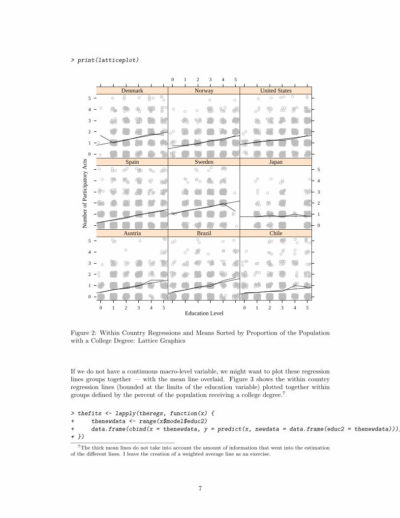
> print(latticeplot)

Education Level

Num

ber

of P

artic

ipat

ory

Act

s

●●

●

●●

●●

● ● ●

●●

●

●

●●

●● ●

●

●● ●●

● ●

●

●

●

●

●●

●●

●

●

● ●●●

●

●

●●● ●●

●

●

●

●

●●

●●

●

●

●●

●

●

●

●

●

●

●●●

●

●

●

● ●

●

●

●●

●

●●●●

●

●

●

●

●●

●● ●●

●

●

●●

●

●

●

●●

●●

●

●●

●●

●

●

●

●

●●

●

●●

●

●

●● ● ●

●

●

●

●●

●

●

● ● ●

●

●●

●

●

●

●●

●

●

●

●●

● ●

●

●●

●●

●●●●

●

●

●

●

●

●

●●●

●●

●●●

●

●

● ●

●●

●

●

●

●

●●

●

●

●

●●

●

●●

●

●

●

●

●●

●

●●

●

●● ●

●●

●

●

●●

●●

●

●

●●●

●●●

●

●●●

●

●

●●

●

●

● ● ●●

●

●

●

●

●

●

●

●

●

●

●

● ●

●

●

●●

● ●

●

●

●●

●

●●●●

●

●

●

●

●●

●

●●

●●

●●

●

●

●

●●

●

●

● ●●

●

●●●

●●

●

●

●

●

●●

●●●

● ●

●

●

● ●●

●●

●

●

●

●

●

●

●

●

●●●

●●

●

● ●

●

●

●

●

●

●●

●

●

● ●

●●

●●

●

●●

●●

●● ●●●

●

● ●

●

●●

●

●●

●● ●

●●●

●

●

●

●

● ●

●

●

●

●

●●

●●

●

●

●

●

●

●●

●

●

●

●

●●

●

●

●●●

●●

●● ●●

●

●

●

●●

●●

●

●●●●

●●

●

●

●●

●●

●

●

●

●

●

●

●●

●

●●● ●●

●●●

●

●

●

●

●

●

●

●●●

●

●●●

●

● ●

●

●●

●

●

●

●● ●●●

●●

●

●●

●

●

●

●

●●

●

●●

●●

●

●

●●

●●●

●

●

●

●

●

●

●

● ●

●●

● ●●

●

●●●

●●

●

●

●●

●

●●

●

●

●

● ●

●

●●

●

●●

●●●

●

●

●

●●

●

●

●

●

●

●

●●

●

●

●

● ●●●●

● ●●

●

● ●●

●

●

●

●

● ●

●●

●●

●

●

● ●● ●

●

●●

●●

● ●

●

●

●●● ●●

●●●

●

●

●●

●

●●●

●

●

●

●

●

●

●

●●

●

●

● ●●

●

●●

●

●

●

●

●

●

●●● ●

●

●● ●●

●●

●

● ●●

●●

●

●

●

●

●●

●

●

●

●

●

●

●

●

● ●●

●

●

●

●●

●●

●

● ●●● ●

●● ●

●●● ●

●

●

●

●●●●● ●

●●

●

●●●●

●

●●

●

●●● ●

●

●

●

●●

●

●●

●● ●

●●

●

●●●● ●

●●●

●

●●

● ●●

●

●●

●

●

●

●

●

●

●●

●

●

●●● ●

●●●

●

●

●

●

●

●

●

●

●

●

● ●

●

●

●●

●

●

●

●

●

●

●

●

●● ●

●●

●

● ●● ● ●

●

●

●

●● ●

●● ●●●

● ●

●●●●

●●

●●●● ●

●

●●

●

●

●

●●●

● ●●●●

●

● ●●

●

●

●

●●

●

●●

● ●

●

●

● ●●●

●●● ●

●

●

●

●

●●

●●●

●●●

●

●●

●●

●

●

●●

●

●

●

●

●●●

● ●

●

●●●

●

●

●

●

●

●●

●

●

●●

●

●●

●

●

●●

●

●

● ●●

●

●● ●

●

●

●●

●

●

●●

●● ●

●

●

●●

●

●

●

●

●

●

● ●

● ● ●●

●●

●

● ●●

●

●●

● ●●●● ●

●●

●● ●●

●

●● ●

●

●●

●

●●

●●

●

●

●

●●

●

●

●

●

●

● ●

●

●

●●●●●

●

●●●

●

●

●●●●

●

●●

●

●

●

●

●

●

●

● ●●

●

●

●

●

●

● ●

●

●

●

●

●● ●

●

●●●

●

●

●

●

●●

●

●

●

●

●

●

●

●

●

●

●

●●

●

●●

●●

● ●

●

●

●●

●

●

●

●

●

●

●

●

● ●

● ●

●

●●

●

●

●

●

●●

●

●

●● ●

●

●●●

●●●

●

●●●

●

●●●

●●

●● ●

●

●

●

●●

●

●

●

●

●

●

●

●

●●

●●●

●

●

●● ●

●●

●●● ●●

●

●

●

●

●

●

●

●

●

●

●

●

●● ●

●

●

●

● ●

●●

●

●

●

●

●

●

●

●

●●●●

●

● ● ●

●

●

●

●

●

●

●

●

●

●●

●●

●●

●●●

●

●

●

●●

●

●

●●●

●

●

●●●

●

●

●●

●●●

●

●●●

●●●

●

●

●

●●

●●

●

●●

●

●

●●●

●●

●● ●●

●

●

●●

●

●

●

●

●

●

● ●●

●●

●

●

●

●

●●

●

● ●

●

●

●

●

●●

●

●

●

●

●

●●●

●●

●

●

●

●

●

●

●●

● ●

●●

●

●

●

● ●

●

●●

●

●

●

●

●

●

● ●●

●●

●●

●

●●●●

●

●

●

● ●

●●●

●

●

●●●

●

●

● ●●●

●● ●●

●

●●

●

● ●●

●●

●

●●●

●

●

●

● ●

●●

●

●●

●

●

●●

●

●

●

●

●

●

●

●

●●

●●●

●

●

●

●

●

●

●

●

●

●

●

●●

●●

●

●

●●

●●● ●●

●

●

●●

●

●

●

●

●

●

●

●0

1

2

3

4

5

0 1 2 3 4 5

Austria

●

●

●

●

●●

●

●

●

●

● ●

●

●

●

●

●

●●

●

●

●

●●

●

●

●●

●

●

●

●

●

●

●

●

●

●●

●

●

●

●

●

●

●

●

●●

●

● ●

●

●

●

●●●● ●

●●

●

●

●

●●

●

●

●●

●

●

●● ●

●

●

●

●●

●

●

●●

●

●

● ●

●

●

●

●

●

● ●

● ●●

●●

●

●

●

●

●●

●

●

●●

●●

●

●● ●

●

●

●

●●

●●

●

●

●

●

●

●

●●

●

●

●●

●●

●

●

●●●

●

●

●

●

●

●●

●●

●● ●

●

●●●

●● ●

●

●

●

●●

●

●

●

●

●

●●

●

●●

●● ●

●

●

●● ●

●

●●

●

●●

●

●

● ●

●

●

●

●

●● ●●

●

●

●

●

●

● ●●

●

● ●

●

●

●

● ●●

●●

●●

●● ●

●

●

●

●

●

●

●

●

●●

●

●

●

●

●

● ●

●

●

●●

●

●

●

●

●●

●

●

●

●

●●●

●

●

●●

● ●

●●

●

●

●●

●●

●●

●

●

●● ●

●

●

●

●

●

●

●

●

●

●●

●

●● ●● ● ●

● ●

●

●

●

●●

●

●

● ●●

●

● ●●

● ●

●

●●

●

●

●●

●●

●●

●

●

●●

●●

●

●

●

●

●

●●●●

●

●

●

● ●

●●

●

●

●●

●

●●

●

●

●●

●

●

●●

●

●●

●

●

●●

●● ●●●

●

● ●● ●

●●

●

●

●

●

●

●

●

●● ●

●

●

●●●

● ●

● ●

●

●

●

●

●● ●

●

●

●

●

●

●

●

●●

●●

●

●

●

●

●

●

● ●●

●

●

●

●●

●

●●●

●

● ●

●

● ●●

●

●

●●●

●

●

●

●

●

●

● ●● ●

●

● ●

●

●●

●

●●

●●

●

●

●

●●●

● ●

●

●

●

●

●

●

●●●● ●

●

●

●●

●

●●●

●

●●●

● ●

●

●

●

●

● ●

●

●●

●●

●●●

●●

●●

●●

●●

●

●

●●●

●

●

●

●

●

●

●●

●

●

●

●

● ●

●

●●

●

●

●

●●●

●●

●●

●

●● ●

●●● ●

●

●

●

●

●

●

●●

●

●

● ● ●●

●

● ●

●

● ●

●

●

●

●

● ●

●

●●

●

●

●

●●● ●

●

●

●

●

●

●●●

●

●

●

●

●

●●

●

●

●

●

●

●

●

●

●

●

●

●

●

●

●

●

●

●

●

●

●●●

●

●

● ●

●●

●

●

●

●

●

●

●

●

●

●

●● ●●

●

●

●

●

●

●

●

●●●

●

●

●●

●

●●

●

●

●

● ●

●

●

●●

●

●●

●

●● ●

●

●

● ●

●●

●

●

●● ●

●

●

●

●●●●

●●

●

●

●

●

●

●

●●

●

●

●

●

●

●

●●

●

●

●

●

●

●

●

●

●

●

●

●

●

●

●●

●●●

●

●

●●

●

●

●●

●

●●

●

●

●

●

● ●

●

●●●

●

●●●

●

●●

●

●

●

●●

● ●

●●●

●

●

●●

●●

●

●

●

●

●

●●●

●

●

●●●● ●

●

●

●● ●

●●

●●

●

●

●

●

● ●

●

●

●

●

●●

●●

●●●

●

●

●

●

●●●

●

●●●

●

●●

●

●

●

●

●

●

●

●

●

●

●●●

●

●●

●●●

●

●

●

●

●

● ●

●●

● ●

●

●

● ●●

●

●

●

●

● ●●

●●

●

●

●

●

●

●

●●

●

●●

●

●

●

●

●● ●

●

●

● ●

●

●

●

●

●

●●

●

●●

●

●

●

●

● ●● ●●

●

●●

●

●

●● ●●

●●

●

●

●

● ●●●● ●

●●

● ●

●●

●

●

●

●

●

●

●

●

●

● ●

●

●●

●

●●●

●●

●

●

●

●

●

●

● ●

●

●

●●

●●

● ●

●

●

●

●●

●●

●

●

●

●●

●

●

●

●

●

●

● ●●

●

●

●

●●●

●

●

●

●●

●

●

●

●

●

●

●●

●

●●

●

●

●

●

●

●

●●

●

●

●●

●

●

●

●●

●

●

●

●

●●

●●

●

●

●

●●● ●

●●

●

●●

●

●

●

●●●

Brazil

●

●● ●●

●

●

●●

●●

●● ●● ●●● ●

●

●●

●

●●● ●

●

●●

●

● ● ●●

●●

●

●

● ●●●

● ●●● ●

●●

● ●

●

●● ●● ●●

●

●

●

●●

●●

●

●

●

● ●●

● ●●

●●●

●

●

●●

●

●

●

●

●

●

●

●

●

● ●●

●

●

●

●●● ●●

●●

●●

●

●

● ●●●

●

●

●

●

●●

●

●

●

●●

●

●●

●

●●●●●

● ●●

●

●●

●

●

●

●●●

●

●

●

●

●

●

●

●

● ●●●

●●●

●

●

●●

●●

●

●

●

●

●

●

● ●

●●

●

●●●●

●● ●

●●● ●●

●● ●●

●

●●●

●●

●●

●●

●●●●●●

●

●●●●

●●

●

●

●

●●

● ●

●

●●

●

●

●●

●

●

●●●●●

●

●

●

●●

●●

●●●● ●●●●● ●

●

●

●

●●● ●●●

● ●

●● ●● ● ●●●● ●

●●

●

●

●

●

●

●●

●●●

●

●●

● ●

●

●

● ●●●

●

●

●

●● ●

●●

●●

●

●●●

●● ●●

●● ●●●

●●

●●

● ●●

●

●●●

●● ●●

●

●

●●

●

●

●●

●●

●

●

●●● ● ●

●

●●

●●

●

●

●

●

●

●●●

●●

●

●

●

●

●●

●

●

●

●

●

●

●

●

●

●

●

●●●

●

●●

●

●● ●● ●

●●●

●

●

●●

●●

●●

●

●

●

● ●●

●●

●

●

●

●

●

● ●

●

●

●

●

●

●●●

●● ●●● ●●

●● ●

●

●● ●

●

●●

● ●●

●

● ●

●● ●

●

●

●

●

●

●●

●

●

●●

●

●

● ●●

● ●●

●

●● ●

●●

●

●

●

●●

●

●●

●

●●● ●

●

● ●●●●

●●●

●

●●

●

●●●●

●

●●

●●

●

●●

●

●●●

●

●● ●●

●

●

●

●

●●●●●

●

●

●

●

● ●● ●● ●●

● ●

●

●

●●

●

●●

●

●●

●

●●●●

●

●

● ●

● ●

●

●

●

●●

●

●

●

●●

●

●

●

●●●● ●

● ●

●

●●●● ●●

●

●●●

●

●

●●

●●

●

●

●

●●

●●●●●● ● ●● ● ●

●● ●●

●●

●

●

●

●

●

●

● ●

●

●

●

●

●● ●●

●●

●

●

●

●

●

●

●

●

● ●●●

●●

●●

●●●

●●

●● ●●●

●

●

●●●●● ●

●

●

●●

●●

●

●

●

●●

●

●●●

●

●●●●

●

●●●

●

●

●

●

●

●

●●

●●● ●

●●●

●●

●● ●

● ●● ●●●●●●

●

●

●●

● ●●

●

●

●

●

●

●●●

●

●●●● ●

●● ●

●

●

●

●●●

●● ●

●● ●●

●●●

●●

●●

●

●●●

●

●

●●● ●● ● ●●

●

●

●

●

●

●

●●

● ●

●

●

●

● ●●●●

●

● ●●●●

●●●●

●

●●●●

●●

●

●● ●

●

●

●

●

●

●●●

●

●

●

●●

●

●

●●●

●

●

●

●

●

●

●

● ●●

●●● ● ●●

●

● ●●

●● ●

●

● ●

●

●●

● ●● ●●

●

● ●

●● ●

●●● ●●

●

●

●

●

● ●●●

●● ●

●●

●●● ● ●

●●

●

●

●●●● ●

● ●●

●

●●

●●

●

●●● ●●

●●●

●●●●

●

●

●

●●●

●● ●

●●●

●● ●●

●●●

●●

●●●

●●

● ● ●● ●

●

●

●

●●●

● ●●

●

●● ●●●● ● ●●●

●

●●

●●

●

●

●

●

●

● ● ●●● ●●● ●●● ●●

●●

● ●

●

●

● ●

●●

●● ● ●●● ●●●●●●●●●●● ●●●

●

●● ●●●

●●●

●●●

●

●

●●

●

●

●

●

●●●

●

●

● ●●●

●●

●●●●

●

●●

0 1 2 3 4 5

Chile●

●●●

●

●●

●●

●

●

● ●● ●

●

●

●●●●

●

●●●

●●

●

●

● ●●●●

●

●

●

●

●●● ●●

● ●●●●

●

●●

● ●

●

●●●

●

●● ●

●●

●

●

●

●●

●

●●●●●

●

●

●

● ●● ●●

●

●

●

●●●

●● ● ●●

●●

●

●

●

● ● ●●●●

●

●

●

●

●●●

●

● ●

●

●

●●●

●

●● ●

●

●●

●

● ●

●●

●●●

●●●●●

●

●●●

● ●

●

●●

●

●

●

●

●●●

●●

●●

● ●

●

●●●●

●

●●● ●

●

●

● ●● ●●

●●

●

●

●

●

●●● ●

●● ●●● ●

●

●●

●

●

●

●● ●● ● ●

● ●● ●

●●● ●●●● ●●●● ●

●

●

●● ●

●

●

●

●

●

●

●

●

●

●

●

● ●●

●●

●●●

●●

●●

●

●

●●

●●

●●●

●

●

●

●● ●

●

●

● ●

●●

●

●

●

●●

●●

●●

● ●

●

●●

●●

●

●

●● ●

●●

●● ● ●●

●●

●●●●

●

●

● ●●●

●

●

●

●

●

●

●

●

●

●

●

●●

●●●

●

●

●

● ●●●● ●●●

●●

●

●●

●

●

●●

●

●

●

●●

●●

●

●●●

●●● ●

●●

●●●

●●

●●

●

●●

●●● ●●

●

●

●●

●

●

●●

●

●● ●

●

●●●●

●●

●● ●

●

●

●●●

●

●

●

●

●

●●

●

●●

●●

●●

●●●

●

●

●●

●

●

●● ●●

●●

●

●●

●

●

●

●

●

●

●

●

●

●

●

●

●

●●

●●

●

● ●●●

●●●

●

●

●

●●

● ●

●

●

●

●

● ●

●

●

●●

●●● ●●

●●

●●●●●

●

●●

●

●

●●●

●● ●

●

●

●●● ● ●

●

●●

●

●●

●

●●●● ●●

●

●

●●

●● ●

●

●

●●

●

●●

●● ●

●

●

● ●●

●

●

●

●

●

●

●●

●

●

●●

●●

●●●●●

●

●

●

●

● ●● ●

●

●

●●

●●

●

● ●

●

●●●●●

●

●

●

●

●● ●●

●

●●●

●

●

●

●

●

●●●

●

●

●

●

●

●

●

●

●

●

●

●

●

●●

●

●

●

●●

●

●

●

● ●

●

●●●

●

●●

●

● ●

●●●●

●●

●

●●● ●

●●

●

●

●

●

●

●● ●●● ●● ●

●

●●

●

●

●

●●●●

●

●●●● ●

●

●

●●

●

●

●

●●

●

●

●

●●

●●

●

●●

●

●

●

●

●

●

●

●

●

●

●

●●● ●

●

●

●●

●●

●● ●

●

●

●

●

●●● ●● ●

●

●

●

●

●

●●

●

●

●

●

●

●

●●

●●

●

●●

●

●

●●

●●●

●●

●

●

●

●

●

●

●

●

● ●

●

●

●● ● ● ●●

● ●●●

●

●

●

●

●

●

●

●●

●●●●●

●● ●

●

●

●●● ● ●

●

●

●

●

●

●●● ●

●

●●

●

●● ●

●

● ●

●

●

●

●

●

●

●

●

●

●●

●●

●● ●

●

●●●

●●

●

●

●

●

●

●

●

●

●

●●

●

●

●

●

●

●●

●

●

●

●

●

●●

●

●

●● ●● ●●●

●

●

●●

●

●

●

●

●

●●

●● ●

●

●●

●● ●●

●●●●

●●

●●●●

●●● ●

●

●

●

●●

● ● ●●● ●●●●●

●●

●●●

●

● ●● ●

●

●●

●

●

●

●

●●

●

●

●

●

●●

●●

●●

●

●

●

●● ●●

●

●

●

●● ●● ●

●

●

●

●●

●

●

●

●

●

●

●

●

●

●

●

●●

●●

●●●● ●

●

●

●

●●

●

●

●

●●

●

●●

●●

●

●

●

●●

●

●●●●

●

●●

●

●●

●●●●●

●●● ●●

●●●●●●

●

●

●

●

●

●

●

●●● ● ●● ●

●

●●

● ●● ●●

●

● ●

●

●

●● ●

● ● ●

●

●

●

●●

● ●

●●

●●

●●

●

●

●

●

●

●

●●

●

●

●

●●

●

●

●

●

●

●

● ●● ●●

●●

●● ●●● ●

●

●

●

●●

●

●

●

●

●

●● ●

●

●

●

●

●●

●●

●

●●● ●●●● ●● ● ●

●●

●

●

●

●

●●

●

●

●

●

●●

●

●

●

● ●●●

●●●

● ● ●●●

●●

●

●●

●

●●

●

● ●●

●

●

●

●

●●

●

●●

●

●

●● ●

●

●

● ●●

●

●●●

●

●

●● ●

●

●

●

●

●

●

●

●

●

● ●

●●●●

●●● ●●

●● ●●●

●● ●

● ●●●●●

●●●

●

●●

●

●●

●

●

●

● ●

●

● ●●

●

●●

●●●

●

●●

●●

●

●

●

●

● ●

●●

●

●● ●

●

●

●

●

●● ●●

● ●

● ● ●●

●● ●

● ● ●

●

●

●●

●

●

●

●● ●

●

●

●

●

●

●

●

●●●

●

● ●●

●

●

●

●

●

●

●

●●●●●● ●●

●●●

●

●

●

● ●●●

●

●●●

●

●

●

●

●● ● ●●● ●●

●●●●

●

●●● ●

● ●● ●

●●

●●

●●● ●

●

●●

●

●●

●

●●

●

●

● ●●

●

●

●

●

●●

●

●

●●● ●

●

●

●

●●●

●

●

●

● ●

●

●

●

●

●

●

●

●

●

●

● ●

●

●

●

●

●●

●

●●

●

●

●

●

●

●

●

●

●

●

●

●

●●● ●●

●●●

●●

●

●

●

●

●

●

●

●

●●

● ●●

●

●

●●

●

●●● ● ●● ●

●●● ●

●

●●●

●●

●●●● ●

●●●

●●●●● ●●●

●●●●

●● ●●●

●

●●

●

●

●

●

●●

●

●

●

●

●●

●

●●

●●

●●●

●

●

●

●

●

● ●

●

●

●

●

●

●● ●

●

●

●

●

●●

●●● ● ● ●

●

●

●

●

●

●

●●●●

●●●

● ●

●

●

●

●

●

●

●

●

●

●

●

●

●

●

●

●

●

● ●●● ●●●

●

●

●

●

● ●●

●

● ●

●

●●

●●

●●●● ●● ●●● ●●●

●●●● ●

●

●●

●●

●

●

● ●

●●

●

●

● ●

●

●

●●●

●● ●

●

● ●●

●

●● ●

●

●●

●

●●

●

●

●●

●

●

●●

●●

●●

●

●

●

●●

●

●

●

●

●

●

●

●●●

●●●●●

●●●

●

●●

●

●●

●

●

●●

●●

●

●●● ●●●

●

●

●

●

●

● ●

●

●

●

● ●●

●

●●●●●

●

●

●

●

●

●

●

● ●●● ●● ●

●

●

●

●●

● ●

●

●

●

●

●

●

●

●

● ●

●

● ●

●●

●

● ●

●●

●●

●●

●● ●

● ●●● ●●

●

●

●

●●

●

● ●

●

●

●●

●●

●●● ●

●

●●

●●● ●● ●

●

●

●

●

●●

Spain

●

●● ●● ●

●

●● ●●

●

●●

●

●

●

●

●

●●●●

●●

●

●

●

●

●

●

●

●

●

●●●

●

●●●

●

●

●●

●

●

●

●●

●

●

●

●

●

●

●

●●

●

●

●

●●

●

●

●●

●

●

●

●

●

●

●

●

●

●

●

●

● ●

●

●

●

●

●

●

●●

●

●●

●

●●

●

●

●●

●

●

●

●●●

●

●

●

●●

●

●

●

●

●

●

●

●

●

●

●

●

●

●●

●

●●

●

● ●● ●

●

● ●

●

● ●●

●

●

●

●●

●

● ●

●

●●

●

●

●

●

●

●

●

●●

●

●

●

●

●

●

●

●

●

●

●

●

● ●

●

●

●●

●

●

●

●

●

●

●

●●

●

●

●

●

●

● ●

●

●

●

●

●●

●

●

●

●●

●

●

● ●

●

●

●●

●

●

●

●

●

●

●●

●

●

●

●● ●

●●

●●●

●

●

●●

●

●

●● ●

●

●

●

●

●

● ●

●

●●

●●

●

●

●

●

●●

●

●

●●

●●

●

●

● ●●●

●

●

●

●

●

●

●

●

●

●●●

●

●

●

●

●●

●

●

●

●

● ●

●

●● ●

●

●●

●

●

●

●

●

●

● ●

●

●

●

●

●

●

●

●

●

●●

●

●●

●

●

●

●

●

●

●

●

●

●

●●

●

●●

●

●

●

●

● ● ●

●●

●

●

●

●

●

●●

●

●

●●

●

●

●

●

●

●●

●

●

●●

●

●

●

●

●

●

●

●●

●

●

●

●

●●

●

●

●

●

●

●

●

● ●●●

●●

●

●

●

●●●●

●

●●●

●

●●●

●

●

●

●

●

●

●

● ●

●●

●●

●

●●

●●

● ●

●●

●

●

●

●

●

●

●

●

●

●

●● ●

●

●

●●

●

●

●

●

●●

●

●●

●

●●

●●

●●

●

●● ●

●

●

●●

●

●

●

●

●●

●

●

●●

●

●

● ●

●

●

●

●

●

●

●

●

●

●

●

●

●●

●

●●●

●

●●●

●

●

●●

●●●

●

●●

●

● ●

●● ●

●

●

●

●

●

●

●●

●

●

●

●

●

●

●

●

●●

●

●

●

●

●

●

●

●

●

●●

●

●

●

●

●●

●●

●

●

●●●

●●

●●

● ●●

●

●

●

●

●

●

●

●

●●●

●

●

●●

●

●

●

●

●

●

●

●

●

● ●

●●●

●●

●●●

●

●

●

●

●

●

●

●

●

●

●

●

●

●

●

●

●

●●

●

●

●

●

●●

●●

●

●

●

● ●

●●

●

●

●

●

●● ●

●

●

● ●

●

●●

●

●

●

●

●

●

●●

●●

●

●

●●

●

●

●

●

●

● ●●

●

●

●

●

●●

●

●

●

●

●

●

●

●

● ●

●

●●

●

●

●●

●

●●●●

●

●

●●

●

●●

●

●

●

●●

●

●

●

●

●

●

●●

●

●

●●

●●

●

● ●

●●

●

●

●●●●

●

● ●

●

●

●

●●

●

● ●

●

●●

●●

●

●

●

●

●

●

●

●

●

●

●●●

●

●●●● ●

●

●

●●

●● ●● ●

●

●●

●

●

●

●●●●●

●

●

●

●

●

●

●

●

●

●

●

●

●

●

●

●●

● ●●

●● ● ●

●

●

●

●● ●

●

●

●

●

●

●

●

●

●

●

●●

●●

●

●

●

●

●

●

●●

●

●

●

●

●

●●●● ●

●

●

●

●

●

●

●

●

●

●

●

●

●

●● ●

●

●●●

●●

●

● ●

●

●

●

●

●

●●

●●●

●

● ●

●

●

●

●

●

●●

●●

●

●●

●

●

●● ●

●●

●●

●●

●●

●

●

●●

●

●

●

●●

●●

●

●

●

●

Sweden

● ●

●

●

●

●

●

● ●● ●

●● ●

●

●●

●

●●

●●

●

●●●

●

●●

●●

●

●

●

●

●

●

●

●

●

●●

●

●

●

●

●

●

●

●

● ●

●●

●●

●●●●

●

●

●●

●

●●

●

●

●

●

●●

●

●●

●●

●

●●

●

● ●

●

●●

●

●

●●

●

●●

●

●

●

●

●

●●●

●

●●●●

●

●

●

●

●

●

●

●

●

●

●

●

●●●

●●●

●●

● ●

●

●

●

●

●

●

●

●

●

●

●

●

●

●●

●

●

●●

●

●

●●●

●●

●●

●

●

●

● ●

●

●

●

●●●

●

●●

●

●

●

●●

●●

●

●

●●

●●

●● ● ●

●

●

●●

● ●

●

●

●

●

●

●

●

●

●

● ●

●

●●

●

●

●

● ●

●●

●

●

●

●

●●

●

●

●

●

●●

●

●

●●

●

●

●

●

●

●

●

●

●●●●

●

●

●

●●

●●

●

●

●

●

●

●

●

●●

●

●

●●●

●●

●

●

●

●

●

●

●

●

●●

●

●

●

●● ●

●●

●●

●

●

●

●●●

●

●●●

● ●●

●

●●

●

●

●

●●

●

●

●

●

●

●

●●

●●

●

●●

● ●●

●●

●

●●●

●

● ●

●

●●

●

●

●

●

●●

●

●

●

●

●

●

●

●●

●● ●

●

●●●

●

●

●●

●● ●

●

●

●

●

●

●

●

●

●

●

●

●

●

● ●●● ●

●

●

●

●

●● ●

●●

●

● ●

●

●

●●

●●

●

●

●

●●●

●●

●●

●

●●●

●

●●●

●

●

●●●

●

●●

●●

●

●

●

●

●

●

●

●

●

● ●

●●

●

●

●●●

● ●

●

●

●●

●●

●

●

●●

●●

●● ●● ●●●

● ●● ●

●●

● ●

●

●

●

●●

●

●●

●

●

●

●● ●

●

●

● ●

●

●

●

●●

●

●

●

●

●

●

●

●

●●

●

●

●

●

●

●

●

●●

● ●●

●

●

●

●

●

●

●

●●

●

●

●

●●

●

●

●

●

●●

●

●

●

●● ●●

●

●

●

●

●

●●

●

●

●●● ●

●

●● ●

●

●

●

●

●●

●

●

●

●

●

●

● ●

● ●●●

●

●

●

●●●●

●●

●

●

●

●●●

● ●

● ●●

●

●

●●

●

●

●

●

●●

●●

●

●

●

●

●

●

●

●

●

●

●●

●●

●

●● ●

● ●●

●

●

●

●

●

●

●

●

●

●●

●

●●● ●

●

●

●●

●

●●

●● ●

●

●●

●

●●●

●

●

●

●

●

●●

●

● ●

●

●

●●

●●

●

●

●

●

●●● ●

●

● ●●●

●

●

●

●

●

●

●●

●●

●

●●● ●●

●

●●

●

●

●

●

●

● ●●

●

●

●●

●●

● ● 0

1

2

3

4

5

Japan

●

●

●

●

●

●

● ●

●

●

● ●

●

●

●

●

●

●

●

●

●

●

●●

●

●

●

●

●

● ●

●

●

●●

●●

●

●

●

●

●

●

●

●

●

●

●

● ●

●

●

●

●●

●

●

●

●●●

●●●

●

●

●

●

●●

●

●

●

●

●

●

●

●●

●

●

●

●●

●

● ●

●

●

●●

●●

●●

●●

●●

●

●●

●

●

●

●●

●

●

●●

●

●●

●

●

●

●

●

●

●

●

●

●● ●

●●

●●

●

●

●●

●●

●

●

●

●

●

●

●

●●

●

●

●

●●

●

●

●

●

●

●●

●

●

●

●

●

●

●

●

●

●

●

●

● ●

●

●

●

●

●

●

●

●

●

●

●

●

●

●

●

●

●

●●● ●●

●

●●

●

●

●●●

●

●

●● ●

●●●

●

● ●●

●

●

●

●

●

●

●

●●

●

●

●●

●

●

●

● ●

●

●

●

●

●

●

●●

●

●

●

●

●

●

●

●●

●●●

●

●

●

●

●

●

●

●

●●●

●

●

●

●●●

●

●

●●

●

●

●

●

●

●

●

●

●

●

●

●

●

●

●

●

●●

●

●

●

●●

●

●

●●●

●

●

●●

●

●

●

●

●

●

●

●●

●

●

●●● ●

●

●●

●

●●

●●

●

●

● ●

●

●●

●

●

●

●

●

●

●

●

●

●

●

●

●

●●

●

●

●

● ●

● ●

●

●

●

●

●

●

●

●●

● ●

●

●

●

●

●●

● ●

●

● ●

●

●●

●●●

●

●●

●●

●

●●

●●

●

●

●●

●

●

●

●

●

●

●

●

●

●

●

●

●

●●

●

●●

●

●

●

●

●

●●

●

●

●

●

●●

●

●

●

●●

●

●

●

●●●

●

●

●

●

●

●

●

●●

●●

●

●

●

●

●

●

●

●

●

●

●

●

●

●

●

●

●●

●

●

●

●

●

●

●

●

●

●

●●

●

●

●

●

●

●●

●

●● ●

●

●●

●

●

●●

●●

●

● ●●

●

●

●●

●

●●

● ●

●● ●

●

●

●●

●

●

●

●●●

●

●

●

●

●●

●

●

●

●

●

●

●

●

●

●●

●

●

●

●

●

●●●

●●●

● ●●

●

●

●

●

●

●

●

●

●

●

●

●

●

●●●

●

●

●

●

●

●●

●

● ●

●

●

●

● ●

●●

●

●●

●

●

●

●

●

●

●●

●

●

●

●

●

●

●

●● ●●

●

●

●

●

●

●

●

●●

●

●●

●

●

●●

●●

●

●

●

●

●

●●

●

●

●

●

●

●

●

●

●

●

●

●

●

●

●

●

●

●

●

●

●

●

●

●●

●

●

●

●

●

●

●

●

●●

●●

●

●

●

●

●

●

●

●

●●

●●

●

●●●

●

●

●

●

●

●

●

●

●

●

●

●●

●

●●

● ●●

●

●

●

●●

●

●

●

●

●

●

●

●

●

●

●

●

●

●●●

●●

●

●

●

●

●

●

●

● ●

●

●

●

●

●

●

●

●●

●

●●

●

●

●

●

●

●●

●●●

●

●

●

●

●

●

●

●

●

●●

●

●

●

●

●●

●

●

●

● ●● ●

●

● ●

●

●

●

●

●

●●●●

●

●

●

●

●

●●● ●

●

●

●

●

●● ●

●

●

●

●

●

●

●

●●●

●

●

● ●●

●●

●

●

●

●

●

●

●

●

●

●

●

●●

●

●

●

●

●●

●

●

●

●

●

●●

●

0

1

2

3

4

5

Denmark

●

●

●● ●

●

●

●

●●

●

●●●

●

●

●

●

●●

●

●●

●

●

●

●

●

●

●

●

●

●● ●

●

●

● ●

●●

●

●●

●

●

●●

●

●

●● ●

● ● ●●●

●●

●●●●

●

●

●

●●

●

●

●●

●

●

●

●

●● ●●

●

●

●● ●●●

●

●

●●

●

●

●●

●

●

●

●●

●

●

●

●●

●

●

●

●

●

●

●

●●

●

●

●● ●

●

●●●

●●

●

●

● ●

●

●

●

●

●●● ●●

●

●

●

●

●●●

●

●●

●

●

●●●

●

●

●

●●

●●

●

●

●●

● ● ●

●

●

●

●

●●●

● ●

●

●●

●

●

●

●

●

●

●

●

●

●

●

●

●

●

●

●

●●

● ●●

●

●

●

●

●

●●●

●

●

●

●

●

●●

●

●

●

●

●

●

●

●

●

●

●

●

●

●

●

●

●

●

●

●

●

●

●●

● ●●

●●

●

●

●

●

●

●

●

●

●

●

●

●●

●

● ●

●

●●

● ● ●●

●

●

●

●●

●

●

●

●

●

●

● ●

●

●

●●●

●

●●

●

●

●

●

●●

●●

●

●

●

●●

●

●

●

●

●●

●

●

● ●

●●

●

●

●

●●

●

● ●

● ●

●

●

●●●

● ●

●

●

●

●

●

● ●

●

●

● ●

●

●

● ●●

●

●

●

●

●●●

●

● ●●

●

●

●●

●

●

●●

●● ●

●

●

●

●

●

●

●

●●

● ●

●

●

●

●

●

●

●●

●

●

●

●

●

●

●●

●●

●

●

● ●●

●●

●

●

●

●●

●

●●

●

●

●●

●

●

●

●

●●●

●●

●

●

●

●

●●

●

●

●●

●

●

●●

●

●

●●

●●

●

●●

●

●

●●

●●

●

●●

●

●●●

●●

●

●

●

●

●

● ●●

●

●

●

●

● ●

●

●

●

●

●

● ●●

●

●

●●

●

●

●

●

●

●

●

●

●

●

●

●

●

●

●

●

●

●

●● ●

●●●

●

●

●

●

●

●

●

●●

●●

●

●

●●

●●

●●

●

●

●

●

●

●

●

●●

●

●

●●

●

●●

●

●●

●●

●

●

●

●

●

●

● ●

●

●

●

●

●●

●

●

●

●

●

● ●●

●

●

●

●

●

●

●

●

●

●

●

●

●

●

●

●

●●● ●●

●

●

●

●

●

●

●

●

●●

●

●

●●

●

●

●

●

●

●●

●

●●

●

●

●

●

●

●

●●●

●

●●

●

●●

●

●●

●

●

●

●

●

●

●

●

●

●

●

●●

●

●

●

●

●

●

●

●●

●

●●

●

●

●●

●

●

●

●

●●●

●●●

●

●

●

●

●

●

●●●

● ●

●●

●

●

●

●

●

●

●

●●

●●

●●

●●●

●

●

●

●

● ●

●●

●

●

●●●

●

●

●

●

●●

●

●●

●●

●

●

●

●

●

●

●●●

●

●

●

●

●

● ●

●

●

●

●

●

●

●

●

●

●

●

●

●

●●

●

●●

●

●

●

●

●●

●

●

●

●●

●

●●

●

●

●

●

●●

●

●

●

●●

●

●●

● ●

●●●

●

●

●●

●

●

●

●●●

●●

●

●

●

●●●

●

●●

●

●

● ●

●

●

●

●

●

●

●

●

●

●

●

●●●

●

●●

●

●

●

●

●

●

●

●●

●

●

●

●

●

●

●

●

●●

●

●

●

●

●●

●

●

●

●

●

●

●

●

●

●

●

●

●

●

●●

●

●

●

●

●

●

●●●

●

●

●●

●

●

●

●●

●

●

●

●

●●

●

●

●

●● ●

●● ●

●

●●

●●

●

●

●

● ●

●

●

●●

●

●

●

●

●

●

●

●

●

●

●

●

●

●●

●

●

●

●

●●

●

●●

●●

●●

●

●

●

●

●

●

●

● ●●

●

● ●●

●

●

●

● ●●

●

●

●

●

●

●

●

●

●

●

●

●

●

● ●

●

●

●

●●

● ●●

●●

●

●●

●●

●

●

●●

●

●●

●

●

●

●

●●

●

●

●

●●●

●

●

●

●

● ●

●

●●

●

●●

● ●

●

●●

●

●●

●●

●

● ● ●

●

●

●

●●

●

●●

●

●

●

●●

●

●

●

●●

●●

●

●●

●●

●

●●

●

●

● ●

●●

●

●

●

●

●

●

●●

●

●

●●

●

●

Norway

0 1 2 3 4 5

●

●

●

●●

●●

●

●

●

●●

●●

●

●

●●

●

●

●

●●

●●

●

●

●●

●

●●

●● ● ●

●●●●● ●

●

●

●●

●

●

●

●

●

●

●

●

●

●

●●

● ●

●

●

●

●

●

●

●

●

●●● ●

●

●

●

●●

●

●

●●

●

●

● ●

●

●

●●

●

●

●●

●

●

●

●

●

●

●

●

●

●

●

●

●

●

●●

●●●

●

● ●●

●

●

●

●●

●●

●●

●

●

●

●●

●

●

●

●

●

●

●

●

●

●●

●

●

●●

●●●

●●

●

●

●● ●

●

●

●

●

●

●●●

● ●

●

●

●

●●●

●

●

●●●●

●

●

●●

●●

●● ●

●

●

●

●

●

●●●

●

● ●●●●

● ●●

●

●

●●

●

●

●

●● ●

● ●●●

●●

●

●

●

●

●

●

●

●

●

●

●

●

●

●

●

●

●● ●

●

● ●● ●

●

●

●

●

● ● ●

●●

●●●

●

● ●●

●

●●

●

●● ●●

●●

●

●

●

●●

●

●

●●

●

●

●

●

●

●

●

●

●

●●

●

●

●

●

●

●

●

●

● ●

●

●

●●

●

● ●

●

●

●●

●

●

●●●

●

●

●

●

●

●●

●

●●

● ●●

●

●

●

●

●●●

●

●

● ●

●

●● ●

●

●

●

●

●

●●

●

● ●

●

●

●

●

●●

●

●●

●●

●

●

●

●●●

●

● ●

●

●

●

●●

●

●

●

●

●● ●

●

●

●●

●

●

● ●

● ●

●

●

●

● ●●

● ●

●

●

●

●●

●

●

●●

●

●●

●

●

●

●

● ●

●

●

●

●

●

●

●

●●●

●

●

●●

●

●

●●

●

●

●

●

●

●

●

●

●●

●

●

● ●

●

●●●

●

●●

●●

● ●

●

●●

●

●

● ●

●

● ●

●

●

●●

●●●

●

● ●●●●

●

●

● ●

●

●●

●

●

●●

●●

●

●●

●

●

●●

●

●

●●

●

●

● ●

●

● ●● ●●

●

●●

●●

●

●

●

●

●●

●

●●

●

●

●

●●

●

●●

● ●●

●

●● ●

●● ●● ●

● ●

●●

●

●

●

●

●

●●

●

●

●

●

●

●●

●●● ●

●●

●●

●

●●●

●

●

●● ●●

●

●●●

●

●●

●

●

●

●

●●

●

●

●● ●

●●●

●

●

●●

●

●

●

●

●

●

●

●

●

●

●

● ●

●●

●

●

● ●● ●

●

●●●

●

●

●●●

●

●

●● ●

●●

●

●

●

●

●

●

●

●

●●

●

●

●

●●

●

●

●●●

●

●●

●

●●

●

●

●

●

●

●●

●

●

●

●

●●

● ●●

●●

●

●●

●

●●

●

●

●●

●

●

●

●

●

●●

●

●

●

●●●●

●

●

●●

●

●

●

●

●

●

●

●

●●●●

●

●

●●

●

●

●

●

●

●

●●

●

●

●

●

●

●

●

●●

● ●

●

●

●

●

●

●

●

●

●

●●

●

● ●

●

●

●

●●

●

●

●

●

●

●

●

●●

● ●●

● ●● ●●

●

●

●

● ●●

●

●

●

●

●●

●

●

●

●

●

●

●●

●

●

●

●

●● ●●

●●

●

●●●

●

●

●

●

●

●

●

●●

●

●

●●

●

●

●●

●

●

●

●

●

● ●●

●

●●●

●

●

●

●

●

●● ●

●

●

●●

●

●

●●

●

●

●●

●

●

●

●

●●●

●

●●● ●●●

●● ●

●

●

●

●

●●●

●●

●●

●●

●

●

●

●

●●

●

●

●● ●

●

●●

● ●

●●● ●

●

●

●

●

●

●

●

●●

●

● ●

● ●

●

●

●

●

●

●● ● ●

●

●

●● ●●●

●

●

●●

●

●

● ●

●

●

●

●

●

●

●

●

●●

● ●

●

● ●

●

●

●

●

●

●

● ●

●●●

●

●●

●

●

●

●

●

●

●

●

●

●

●

●●

●●

●

●

●●●

●

●

●●

●

●●

●● ●

●●

●●●●

● ●

●●

●●

●

●

●

●

●

●●

●

●

●●

●

●●

●●

●

●

● ●

●

●

●

●

●

● ●●

● ●●

●

●

●●

●

●

●●

●

●

●

●

●

●

● ●

●

●

●

●

●

●

●

●

●

●

●●

●

●

●●

●●

●

●

●

●

United States

Figure 2: Within Country Regressions and Means Sorted by Proportion of the Populationwith a College Degree: Lattice Graphics

If we do not have a continuous macro-level variable, we might want to plot these regressionlines groups together — with the mean line overlaid. Figure 3 shows the within countryregression lines (bounded at the limits of the education variable) plotted together withingroups defined by the percent of the population receiving a college degree.7

> thefits <- lapply(theregs, function(x) {

+ thenewdata <- range(x$model$educ2)

+ data.frame(cbind(x = thenewdata, y = predict(x, newdata = data.frame(educ2 = thenewdata))))

+ })

7The thick mean lines do not take into account the amount of information that went into the estimationof the different lines. I leave the creation of a weighted average line as an exercise.

7

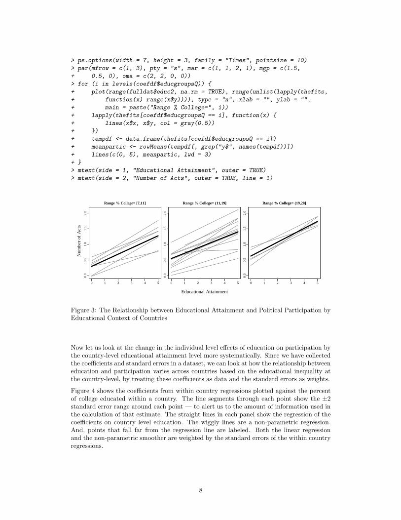
> ps.options(width = 7, height = 3, family = "Times", pointsize = 10)

> par(mfrow = c(1, 3), pty = "s", mar = c(1, 1, 2, 1), mgp = c(1.5,

+ 0.5, 0), oma = c(2, 2, 0, 0))

> for (i in levels(coefdf$educgroupsQ)) {

+ plot(range(fulldat$educ2, na.rm = TRUE), range(unlist(lapply(thefits,

+ function(x) range(x$y)))), type = "n", xlab = "", ylab = "",

+ main = paste("Range % College=", i))

+ lapply(thefits[coefdf$educgroupsQ == i], function(x) {

+ lines(x$x, x$y, col = gray(0.5))

+ })

+ tempdf <- data.frame(thefits[coefdf$educgroupsQ == i])

+ meanpartic <- rowMeans(tempdf[, grep("y$", names(tempdf))])

+ lines(c(0, 5), meanpartic, lwd = 3)

+ }

> mtext(side = 1, "Educational Attainment", outer = TRUE)

> mtext(side = 2, "Number of Acts", outer = TRUE, line = 1)

0 1 2 3 4 5

0.0

0.5

1.0

1.5

2.0

Range % College= [7,11]

0 1 2 3 4 5

0.0

0.5

1.0

1.5

2.0

Range % College= (11,19]

0 1 2 3 4 5

0.0

0.5

1.0

1.5

2.0

Range % College= (19,28]

Educational Attainment

Num

ber

of A

cts

Figure 3: The Relationship between Educational Attainment and Political Participation byEducational Context of Countries

Now let us look at the change in the individual level effects of education on participation bythe country-level educational attainment level more systematically. Since we have collectedthe coefficients and standard errors in a dataset, we can look at how the relationship betweeneducation and participation varies across countries based on the educational inequality atthe country-level, by treating these coefficients as data and the standard errors as weights.

Figure 4 shows the coefficients from within country regressions plotted against the percentof college educated within a country. The line segments through each point show the ±2standard error range around each point — to alert us to the amount of information used inthe calculation of that estimate. The straight lines in each panel show the regression of thecoefficients on country level education. The wiggly lines are a non-parametric regression.And, points that fall far from the regression line are labeled. Both the linear regressionand the non-parametric smoother are weighted by the standard errors of the within countryregressions.

8

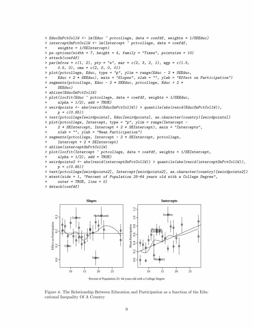
> EducOnPctCollW <- lm(Educ ~ pctcollege, data = coefdf, weights = 1/SEEduc)

> interceptOnPctCollW <- lm(Intercept ~ pctcollege, data = coefdf,

+ weights = 1/SEIntercept)

> ps.options(width = 7, height = 4, family = "Times", pointsize = 10)

> attach(coefdf)

> par(mfrow = c(1, 2), pty = "s", mar = c(2, 3, 2, 1), mgp = c(1.5,

+ 0.5, 0), oma = c(2, 0, 0, 0))

> plot(pctcollege, Educ, type = "p", ylim = range(Educ - 2 * SEEduc,

+ Educ + 2 * SEEduc), main = "Slopes", xlab = "", ylab = "Effect on Participation")

> segments(pctcollege, Educ - 2 * SEEduc, pctcollege, Educ + 2 *

+ SEEduc)

> abline(EducOnPctCollW)

> plot(locfit(Educ ~ pctcollege, data = coefdf, weights = 1/SEEduc,

+ alpha = 1/2), add = TRUE)

> weirdpoints <- abs(resid(EducOnPctCollW)) > quantile(abs(resid(EducOnPctCollW)),

+ p = c(0.85))

> text(pctcollege[weirdpoints], Educ[weirdpoints], as.character(country)[weirdpoints])

> plot(pctcollege, Intercept, type = "p", ylim = range(Intercept -

+ 2 * SEIntercept, Intercept + 2 * SEIntercept), main = "Intercepts",

+ xlab = "", ylab = "Mean Participation")

> segments(pctcollege, Intercept - 2 * SEIntercept, pctcollege,

+ Intercept + 2 * SEIntercept)

> abline(interceptOnPctCollW)

> plot(locfit(Intercept ~ pctcollege, data = coefdf, weights = 1/SEIntercept,

+ alpha = 1/2), add = TRUE)

> weirdpoints2 <- abs(resid(interceptOnPctCollW)) > quantile(abs(resid(interceptOnPctCollW)),

+ p = c(0.85))

> text(pctcollege[weirdpoints2], Intercept[weirdpoints2], as.character(country)[weirdpoints2])

> mtext(side = 1, "Percent of Population 25-64 years old with a College Degree",

+ outer = TRUE, line = 0)

> detach(coefdf)

●

●● ●

●

●

●

●

●

●

●

●

●

●

●

●

●

●

●

●●

●●

●

●

10 15 20 25

0.0

0.1

0.2

0.3

Slopes

Effe

ct o

n P

artic

ipat

ion

Chile

Greece

Japan

Netherlands

●

●

●

●

●

●

●

●

●

●

●

●

●

●

●

●

●

●

●

●

●

●

●

●

●

10 15 20 25

0.0

0.2

0.4

0.6

0.8

1.0

1.2

Intercepts

Mea

n P

artic

ipat

ion

BelgiumGermany

Hungary

Sweden

Percent of Population 25−64 years old with a College Degree

Figure 4: The Relationship Between Education and Participation as a function of the Edu-cational Inequality Of A Country

9

In the slopes panel, we see that the relationship between an individual’s education and herparticipation does not depend in any simple linear way on the percent of the populationwho has a college degree, although there might be some interesting non-linear pattern.Furthermore, we see that Japan is not well characterized by the process that captures theother countries. In the intercepts panel, we see that countries where more people havecollege degrees tend to have higher participation rates among people with low educationalattainment than countries where fewer people have college degrees. In other words, itappears that there is a participation benefit that accrues from living in a place where manypeople have more education — even for people who do not have high educational levels. Bothpanels also alert us to the fact that certain countries do not fit the general patterns very well:Japan stands out for having almost no relationship between education and participation,and Sweden and Hungary are places where those with low education appear to participatemore and less, respectively, than would be expected given the educational context in thosecountries.

So far, it is also clear that people who have more education are more likely to get involvedin petitions, boycotts, demonstrations, illegal strikes, and sit-ins than people who haveless education, in nearly every country in the dataset. This result is surprising given myexpectations about how political institutions (and social status) ought to be differentlyrelated to education in different countries. We have also seen that Japan does not havea pattern like the others. In Japan, in 1999-2001, education did not appear related toparticipation at all. Notice that if we had skipped this plotting step, we would have estimatedsome kind of model that produced a coefficient for something like the “average relationshipbetween education and participation” across countries. This coefficient might have hadmany stars, or not. And, these plots suggest that an average slope might do a good jobsummarizing these patterns (i.e., the slopes do not look that different across countries).However, the lack of relationship in Japan would have been smoothed over. Since this is anarticle about how to use R, I will not speculate about what this result means for Japan or forthe overall question I posed at the beginning of the article. However, it is worth noting thatthe plots have taught us something about the phenomenon we care to understand, whichwould have been hard to pick up in a model specified before looking at the data.

Point 3: Plot to Check Assumptions for Future Modeling

Many popular modeling strategies for multilevel data rely on assumptions about relation-ships between the slopes and intercepts in within country regressions. For example, most“random effects” or “random coefficients” or “multilevel” models (whether estimated usingmaximum likelihood or Markov-Chain Monte-Carlo simulation) assume that the slopes andthe intercepts can be thought of as drawn from a multivariate normal distribution. Howplausible is such an assumption in this case? A priori, it is hard to know. It is plausible thatwe could have some countries with very strong relationships and others with no relationships— leading to a bimodal distribution of slopes. If this were the case, then the assumptionsabout normally distributed random coefficients would not be tenable.

The top row of figure 5 shows qqplots where the slopes and intercepts are plotted againstwhat would be expected, were these variables drawn from a normal distribution. The bottomrow shows the non-parametric density estimates for the slopes and intercepts. Overall, theslopes and intercepts do look like they could have been drawn from a normal distribution,for a few outlying points.

10

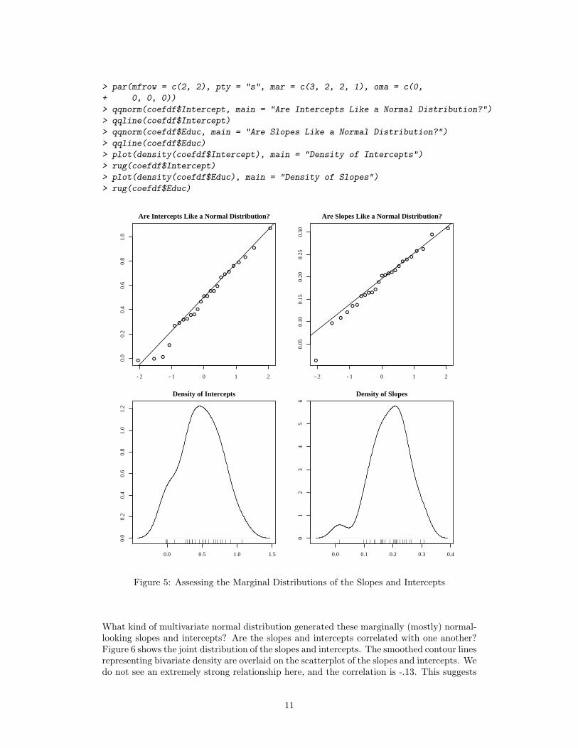
> par(mfrow = c(2, 2), pty = "s", mar = c(3, 2, 2, 1), oma = c(0,

+ 0, 0, 0))

> qqnorm(coefdf$Intercept, main = "Are Intercepts Like a Normal Distribution?")

> qqline(coefdf$Intercept)

> qqnorm(coefdf$Educ, main = "Are Slopes Like a Normal Distribution?")

> qqline(coefdf$Educ)

> plot(density(coefdf$Intercept), main = "Density of Intercepts")

> rug(coefdf$Intercept)

> plot(density(coefdf$Educ), main = "Density of Slopes")

> rug(coefdf$Educ)

●

●

●

●

●

●

●

●

●

●

●

●

●

●

●

●

●

●

●

●

●

●

●

●

●

−2 −1 0 1 2

0.0

0.2

0.4

0.6

0.8

1.0

Are Intercepts Like a Normal Distribution?

Theoretical Quantiles

Sam

ple

Qua

ntile

s

●

●

●●

●

●

●

●

●

●

●

●

●

●

●

●

●

●

●

●●

●●

●

●

−2 −1 0 1 2

0.05

0.10

0.15

0.20

0.25

0.30

Are Slopes Like a Normal Distribution?

Theoretical Quantiles

Sam

ple

Qua

ntile

s

0.0 0.5 1.0 1.5

0.0

0.2

0.4

0.6

0.8

1.0

1.2

Density of Intercepts

Den

sity

0.0 0.1 0.2 0.3 0.4

01

23

45

6

Density of Slopes

Den

sity

Figure 5: Assessing the Marginal Distributions of the Slopes and Intercepts

What kind of multivariate normal distribution generated these marginally (mostly) normal-looking slopes and intercepts? Are the slopes and intercepts correlated with one another?Figure 6 shows the joint distribution of the slopes and intercepts. The smoothed contour linesrepresenting bivariate density are overlaid on the scatterplot of the slopes and intercepts. Wedo not see an extremely strong relationship here, and the correlation is -.13. This suggests

11

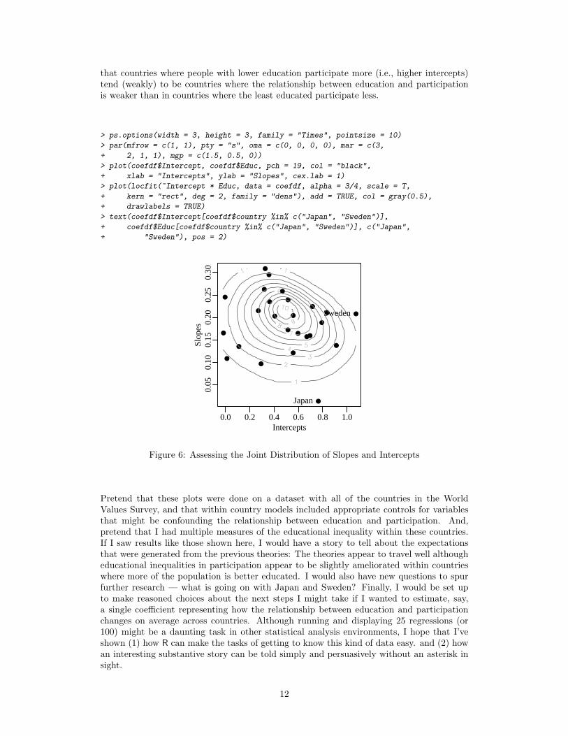
that countries where people with lower education participate more (i.e., higher intercepts)tend (weakly) to be countries where the relationship between education and participationis weaker than in countries where the least educated participate less.

> ps.options(width = 3, height = 3, family = "Times", pointsize = 10)

> par(mfrow = c(1, 1), pty = "s", oma = c(0, 0, 0, 0), mar = c(3,

+ 2, 1, 1), mgp = c(1.5, 0.5, 0))

> plot(coefdf$Intercept, coefdf$Educ, pch = 19, col = "black",

+ xlab = "Intercepts", ylab = "Slopes", cex.lab = 1)

> plot(locfit(~Intercept * Educ, data = coefdf, alpha = 3/4, scale = T,

+ kern = "rect", deg = 2, family = "dens"), add = TRUE, col = gray(0.5),

+ drawlabels = TRUE)

> text(coefdf$Intercept[coefdf$country %in% c("Japan", "Sweden")],

+ coefdf$Educ[coefdf$country %in% c("Japan", "Sweden")], c("Japan",

+ "Sweden"), pos = 2)

●

●● ●

●

●

●

●

●

●

●

●

●

●

●

●

●

●

●

●●

●●

●

●

0.0 0.2 0.4 0.6 0.8 1.0

0.05

0.10

0.15

0.20

0.25

0.30

Intercepts

Slo

pes

Japan

Sweden

Figure 6: Assessing the Joint Distribution of Slopes and Intercepts

Pretend that these plots were done on a dataset with all of the countries in the WorldValues Survey, and that within country models included appropriate controls for variablesthat might be confounding the relationship between education and participation. And,pretend that I had multiple measures of the educational inequality within these countries.If I saw results like those shown here, I would have a story to tell about the expectationsthat were generated from the previous theories: The theories appear to travel well althougheducational inequalities in participation appear to be slightly ameliorated within countrieswhere more of the population is better educated. I would also have new questions to spurfurther research — what is going on with Japan and Sweden? Finally, I would be set upto make reasoned choices about the next steps I might take if I wanted to estimate, say,a single coefficient representing how the relationship between education and participationchanges on average across countries. Although running and displaying 25 regressions (or100) might be a daunting task in other statistical analysis environments, I hope that I’veshown (1) how R can make the tasks of getting to know this kind of data easy. and (2) howan interesting substantive story can be told simply and persuasively without an asterisk insight.

12

References

Cleveland, William S. 1993. Visualizing data. Summit, NJ: Hobart Press.

CSES Secretariat. N.d. “The Comparative Study of Electoral Systems.”.url: http://www.umich.edu/~cses

European Commission. N.d. “Eurobarometer.”.url: http://europa.eu.int/comm/public_opinion/index_en.htm

Huckfeldt, R. Robert. 1979. “Political Participation and the Neighborhood Social Context.”American Journal of Political Science 23(3):579–592.

Inglehart, Ronald, Bi Puranen, Thorleif Pettersson, Juan-Diez Nicolas and Yilmaz Esmer.N.d. “The World Values Survey.”.url: http://www.worldvaluessurvey.org/

Jusko, Karen Long. 2004. “A Two-Step Strategy for the Analysis of Cross-National PublicOpinion Data.” Unpublished manuscript.

Lagos, Marta and The Latinobarometro Corporation. N.d.url: http://www.latinobarometro.org

Nie, Norman, Jane Junn and Kenneth Stehlik-Barry. 1996. Education and DemocraticCitizenship in America. Chicago: University of Chicago Press.

R Development Core Team. 2004. R: A language and environment for statistical computing.Vienna, Austria: R Foundation for Statistical Computing. ISBN 3-900051-00-3.url: http://www.R-project.org

Rosenstone, Steven and John Mark Hansen. 1993. Mobilization, Participation and Democ-racy in America. MacMillan Publishing.

Sarkar, Deepayan. 2004. Lattice Graphics. R Foundation for Statistical Computing. Imple-mentation of Trellis Graphics.url: http://cran.r-project.org/src/contrib/Descriptions/lattice.html

The Afrobarometer Network. N.d. “Afrobarometer.”.url: http://www.afrobarometer.org

Verba, Sidney, Kay Lehman Schlozman and Henry Brady. 1995. Voice and Equality: CivicVoluntarism in American Politics. Cambridge: Harvard University Press.

13